GPC-Based Stable Reconfigurable Control

GPC-Based Stable Reconfigurable Control

Don Soloway Computational Sciences Division

NASA Ames Research Center Moffett Field, CA 94035

Jianjun Shi and Atul Kelkar* Department of Mechanical Engineering

Iowa state University Ames, IA 50010

Abstract

This paper presents development of multi-input multi-output (MIMO) Generalized Pre- dictive Control (GPC) law and its application to reconfigurable control design in the event of actuator saturation. A Controlled Auto-Regressive Integrating Moving Average (CARIMA) model is used to describe the plant dynamics. The control law is derived using input-output description of the system and is also related to the state-space form of the model. The sta- bility of the GPC control law without reconfiguration is fht established using Riccati-based approach and state-space formulation. A novel reconfiguration strategy is developed for the systems which have actuator redundancy and are faced with actuator saturation type fail- ure. An elegant reconfigurable control design is presented with stability proof. Several numerical examples are presented to demonstrate the application of various results.

1 Introduction Over last decade, GPC has emerged as one of the leading control design strategies for robust control of dynamical systems. In early years (prior to late eighties) GPC’s applicability was essentially limited only to process control applications due to its demand on computational speeds. However, with the advances made in the computer technology over last decade computational speed is not a major concern for many real-life applications and control engineers have started using GPC for many main-stream applications. In recent years, GPC has become a viable alternative or in some cases even a preferred choice over well- known H,, Ha, and p-synthesis approaches. GPC has proved to be very effective when requirements on the robustness and performance are hard to achieve with traditional control designs.

GPC belongs to a class of Model Predictive Control (MPC) methods. History of MPC dates back to late 70’s when the process industry showed keen interest in using these control methods. The control formulation at the time was mainly heuristic and algorithmic [l, 21, and exploited the increasing potential of digital processors. These controllers were closely

-related%% which is central to most of the MPC algorithms came about as early as 60’s [3]. As men- tioned earlier, MpCs became quite popular in the process industries where computational

i&=I=I-- . T h e - = k h m . .___ . . -~ __

*Author acknowledges support of NASA Ames Research Center through Grant No. NAGZ-1471

speed was not a major concern. Also, many MPC algorithms were used on multivariable systems with constraints but no formal proofs of stability or robustness were availabie. Another parallel development took place using ideas from adaptive control which led to the development of self-tuning controllers [4] and extended horizon adaptive controllers (EHAC)[5]. This continued evolution of MPCs led to the emergence of the Generalized Predictive Control (GPC) methodology in late 80’s [16] which incorporates all major fea- tures of the predictive controllers in a unified framework. Various versions of the same common idea gave rise to the following different types of predictive controllers: Multi-step Multivariable Adaptive Control (MUSMAR) [6], Multipredictor Receding Horizon Adaptive Control (MURHAC) [7], Predictive Functional Control (PFC) [8], and Unified Predictive Control (UPC)[9].

MPC has also been formulated in the state-space setting [lo], which not only allows the use of well established state-space theories for analysis but also provides the ease for extensions to multivariable systems. Moreover, it facilitates the use of stochastic theories and treatment of actuator/sensor noise. The well developed estimation theory from state space methods can be easily incorporated without much complication. The perspective gained by working in these different domains made it possible to devise some simple tuning rules for ensuring stability and robustness for MPC systems. As a simple analogy, MPC controller can be viewed as an observer-based controller wherein its stability, performance, and robustness is determined by the observer dynamics, which can be fixed by adjustable parameters, and regulator dynamics, determined by MPC parameters such as weightings, horizon lengths, etc. In MPC, the control action at the current time instant is obtained by solving a finite horizon open-loop optimal control problem at each sampling instant. That is, the optimization problem yielding a control input is solved on-line at each time instant. The optimization process at each time instant yields an optimal control sequence and only the first control input in this sequence is applied to the plant. The novelty of MPC lies in its structure and not the control law itself. It essentially solves a standard nonlinear (or linear) optimal control problem. The fact that MPC solves the problem on-line and that it has the ability to naturally and explicitly handle the input and output constraints makes it a popular and powerful control paradigm.

One major criticism of MPC methodology is that, except for some special cases, there is no general purpose theory which guarantees closed-loop stability of MPC. Although, in [Ill, some specific stability theorems are given for GPC using the state-space setting the general case stability results for GPC were lacking. Recently, in go’s, stability of GPC under end-point constraints was shown in [12, 131 where the equality constraints were imposed on the output after at the end of a finite horizon. A variation of this end-point constraint idea is used in this paper for establishing stability of Multi-Input Multi-Output (MIMO) reconfigurable control architecture using GPC. The stability proof uses Linear Quadratic Regulator (LQR) results and monotonicity properties of Riccati solutions. This paper also presents a clean and detailed formulation of GPC prediction equations and derivation for end-point constraint-based GPC control law for MIMO linear time-invariant (LTI) systems. A stable reconfiguration capability of the proposed GPC architecture is demonstrated using a simulation example.

2

I

2

N

1 ‘ 1 I I * t-1‘ t t i l --- t+j --- t+N

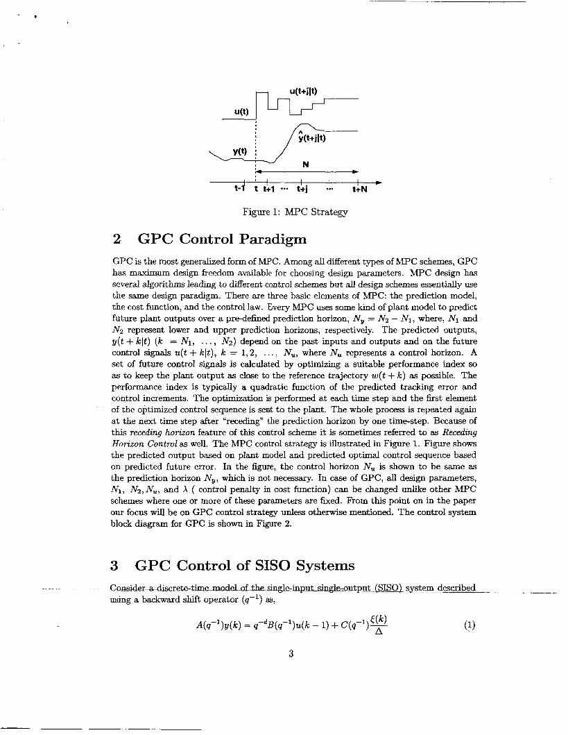
Figure 1: MPC Strategy

GPC Control Paradigm GPC is the most generalized form of MPC. Among all different types of MPC schemes, GPC has maximum design freedom available for choosing design parameters. MPC design has several algorithms leading to diEerent control schemes but all design schemes essentially use the same design paradigm. There are three basic elements of MPC: the prediction model, the cost function, and the control law. Every MPC uses some kind of plant model to predict future plant outputs over a predefined prediction horizon, Ny = NZ - N1, where, N1 and N2 represent lower and upper prediction horizons, respectively. The predicted outputs, y ( t + klt) (k = N1, . . . , N2) depend on the past inputs and outputs and on the future control signals u(t + k l t ) , k = 1,2, . . . , Nu, where Nu represents a control horizon. A set of future control signals is calculated by optimizing a suitable performance index so as to keep the plant output as close to the reference trajectory w(t + k) as possible. The performance index is typically a quadratic function of the predicted tracking error and control increments. The optimization is performed at each time step and the first element of the optimized control sequence is sent to the plant. The whole process is repeated agaiu at the next time step after ‘LTeceding” the prediction horizon by one time-step. Because of this receding horizon feature of this control scheme it is sometimes referred to as Receding Horizon Control as well. The MPC control strategy is illustrated in Figure 1. Figure shows the predicted output based on plant model and predicted optimal control sequence based on predicted future error. In the figure, the control horizon Nu is shown to be same as the prediction horizon N,, which is not necessary. In case of GPC, all design parameters, N1, Nz,Nu, and X ( control penalty in cost function) can be changed unlike other MPC schemes where one or more of these parameters are fixed. From this point on in the paper our focus will be on GPC control strategy unless otherwise mentioned. The control system block diagram for GPC is shown in Figure 2.

3 GPC Control of SISO Systems ~ CoIlsider- adiscrett3=timemodelof_the_smgle-inDntingleoutput (SISO) system described

using a backward shift operator (q-’) as,

(1) A(q-l)y(k) = q - d B ( q - l ) ~ ( k - 1) + C(q- 1 )a

3

cost function Constraints

Reference input output

Optimizer Plant b

I 1 Reference

input output Optimizer Plant b

Model

Figure 2: MPC block diagram

where u(k) and y(k) are the control and output sequences of the plant and ( ( k ) is an uncorrelated random sequence. A, B , and C are the polynomials in the backward shift operator q-':

A(4-l)

B(q-')

=

= 1 + ~ 1 q - l + ~ z q - ' + . . . + anaq-na bo + b1q-l + bzq-' + . . . + b,bq-nb

C(q-1) = 1 + c1q-1 + czq-2 + . . . + c,cq-nc

where d is the dead time of the system. A is the difference operator 1 - 4-l. This model is known as a Controlled Auto-Regressive Integrating Moving Average (CARJMA) model. For simplicity in the development, without loss of generality, C(q-') is chosen to be 1. The plant (1) is then given by:

(2) E ( k ) A ( q - l ) y ( k ) = q - d B ( q - l ) U ( k - 1) + -

[G(k + j ) - w(k + j)I2 +

A The basic cost function used in CPC has the form

N2 NU

j=Ni j = 1 W l , Nz, Nu, A) = A(j )[Au(k + j - I)]' ( 3 )

where, G(k + j) is an optimum j-step ahead prediction of the system output up to time k , w(k + j ) , j = 1 , 2 , . . . is a future set-point or reference sequence. N1 is the minimum prediction horizon, N2 is the maximum prediction horizon, Nu is the control horizon and A(k) is a control-weighting sequence. As seen in Eq. (3) , the cost function is quadratic and penalizes future tracking errors over prediction horizon and control energy over control horizon. It is assumed that the control increments after control horizon are zero. The basic idea is to compute the optima2 future control sequence, ??*(IC) = [u(k) , u (k + l), . . .], such that the cost function J ( N l , N2, Nu, A) is minimized. The control designer has to select the tuning parameters, N1, N2, Nu, and A, to meet certain stability and performance objectives. Once ~ * ( k ) is computed, only the first element of the sequence is used and the whole process is repeated at next time step.

3.1 Prediction of future outputs In order to compute the cost function, which consists of future tracking errors, we need to compute the future outputs, y^(k + j ) (Nl 5 j 5 NZ) , using the best available plant

4

- 1

model (2). In case of SISO systems, these predictions can be easily computed using the Diophantine equation [9]. The development of prediction equations for SISO case using Diophantine approach is detailed in the Appendix 3.1. The prediction equations obtained in section 3.1 using Diophantine approach are very cumbersome to use and are not easily extendable to MIMO case. This motivates the development of state-space based formulation of prediction equations and control law.

3.2 State-space formulation of prediction equations Consider a state-space description of the plant (Eq. 1) given as:

~ ( k + 1) = Ax(k) + BAu(k) + B.&(k) Y(k) = W k ) +m)

(4)

The reason for using the state-space form of the system with Au(k) as input is that the algebraic complexity in the derivation of GPC control law reduces significantly in this form. The transformation of system equations with u(k) input to this form is given in detail in the appendix. In Eq. (4), the dimension of state vector is n = muz(n, + 1, nb + d + 1, nc), and matrices A.

A =

3 , Bf, and C are given

-zn 0 0 - . * 0

Y

B =

0 0

b0

bn-d-1

bnb-d-1

C = [ l 0 ... 0 ... 0 ...I

where Zt axe the coefficients of polynomial 2, which is given by

(5 ) -(na+l) X(q-l) = AA(q-l) = 1 + iT1q-l + . . . + ?inq-n + . . . + Z,+lq ~ - ~

Note that, in matrix B, the d leading elements are zeros. T&E&dZi@EE %p-lon of CAFUMA model is shown in Fig. 3. If d = 0, the CARTMA model representation becomes that of Fig. 4. If in addition to d = 0, C(q-') = 1, the CAlUMA model takes the form of Fig. 5, For both cases of Figs. 4 and 5, we can get the corresponding state-space

5

I

......

-T ..

t 7- ...... ...... I ...... I I I

Figure 3: The CAMMA model

5(k) ...... ~ ...... ~

I I I ...... ......

Figure 4: The CAlUMA model with d = 0

model. As mentioned previously, since the noise and disturbances in future are not known apriori

for prediction of future outputs only deterministic part of the plant model is considered in the following development. The deterministic part of plant dynamics in polynomial description is given by

A(q-')Ay(k) = B(q-')Au(k - 1) ( 6 )

Let the corresponding state-space model be

Using the z-transform, we can obtain the z-domain transfer function H(z) as follows:

- C(I - +)-IB -

z

6

...... ...... 5 ( k )

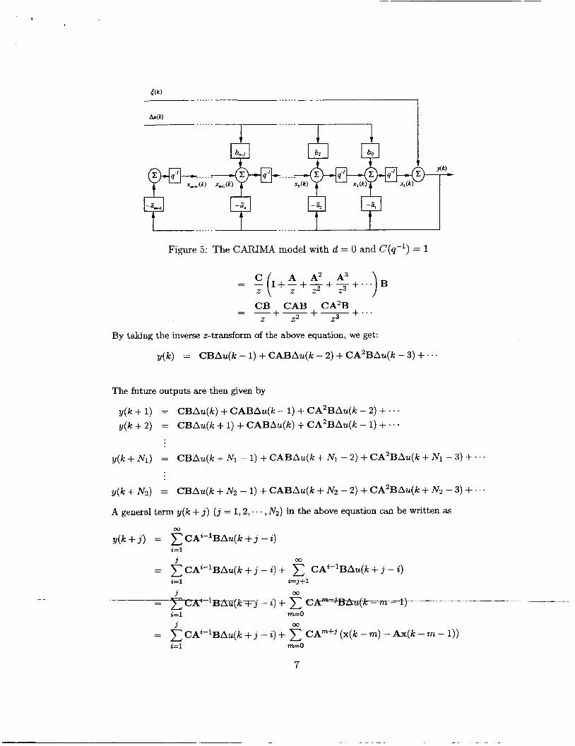
Figure 5: The CAMMA model with d = 0 and C(q-') = 1

A A2 A3 z

CB CAB CA2B - - - +-+-+... Z 22 z 3

By taking the inverse z-transform of the above equation, we get:

y(k) = CBAu(k- l )+CABAu(k- 2)+CA2BAu(k - 3 ) + - . -

The future outputs are then given by

Y(k + 1) = CBA+) + C A B A ~ ( ~ - 1) + C A ~ B A ~ ( ~ - 2) + . . . y(k + 2) = CBAu(k + 1) + CABAu(k) + CA2BAu(k - 1) + . . .

y(k + N1) = CBAu(k + N1 - 1) + CABAu(k + N1 - 2) + CA2BAu(k + N1 - 3) + .. .

y(k + N2)

A general term y(k + j ) ( j = 1,2 , . . . , N2) in the above equation can be written as

= CBAu(k + N2 - 1) + CABAu(k + N2 - 2) + CA2BAu(k + N2 - 3) + . . .

m

y(k + j ) = CA*-~BAU(~ + j - i) i=l j W

= C A ~ - ~ B A ~ ( ~ + j - i) + C C A ~ - ~ B A Z L ( ~ + j - i ) i=l i=j+l

j M

i=l m=O = C A ~ - ~ B A ~ ( ~ + j - i) + C C A ~ + ~ ( ~ ( k - m) - AX@ - m - 1))

7

j 00

= C C A Z - ~ B A ~ ( ~ + j - i) +

=

C A ~ ( ~ ~ x ( k - m) - ~ m + l x ( k - m - 1)) J i=l m=O j

i=l C A Z - ~ B A ~ ( ~ + j - i) + C A ~ X ( ~ )

Now using assumption of GPC control strategy that Au(k+i) = 0 for i 2 Nu, and denoting

we can write the predicted output as

where

3=

and G is given by

G =

CA CA2 1

CANZ ]

Note that Eq. (8) allows easy computation of G compared to Diophantine-based technique. For SISO systems, it is interesting to note that the polynomials Ej and Fj in Diophantine equation solution have coefficients that relate to the A matrix of the state-space form of Eq. (4). To be specific, the elements in the first row of Aj are the last ?tu cueEcieiits of Ej+l in the decreasing order of the degree of 4-l and the first column has the coefficients of Fj in the increasing order of the degree of 9-l.

~ ~~ ~~ -~

3.3 Development of GPC for MIMO Systems In this section, we will develop GPC control law for the general case of MIMO LTI systems. For algebraic simplicity we will use state-space description for plant dynamics. Let the

8

,

state-space model for a general MIMO system with p inputs and q outputs is given by

~ ( k + 1) = Ax(k) + BAu(k)

Y ( k ) = Cx(k) (9)

where, x is the n-dimensional state vector, A, B and C are system matrices with dimensions n x n, n x p , and q x n, respectively.

The cost function to be minimized is given by

Nz J(N1, N2, Nu, A) = c (Y(k + j ) - w(k + + j ) - w(k + A ) +

j=Nl

NU X(Au(k + j - l))T(AU(k + j - 1)) (10)

j=1

where, y is the q-vector of predicted output, w is the q-vector of reference trajectory, and AU is the pvector of input increments. In order to compute the optimal control input minimizing above performance function output predictions need to be computed over the prediction horizon. The following section develops prediction equations for MIMO case.

3.4 The procedure developed for predicting output in SISO case can be extended to MIMO systems as well with some added algebraic complexity. Consider a MIMO system of Eq. (9). We can compute the future outputs y ( k + j) ( j = 1,2, . . + , N1,. . . , N2) based on the plant information available up to time k using a recursion procedure. The predictions of state for future times starting at time k are given by

Output prediction for MIMO Systems

x(k + 1) = Ax(k) + BAu(lc) xjk + 2) x(k + 3)

=

= Ax(k + 1) + BAu(k -k 1) = A2x(k) t- ABAu(k) + BAu(k + 1) Ax(k + 2) + BAu(k + 2) = A3x(k) + A2BAu(k) + ABAu(k + 1)

+BAu(k + 2)

j-1

x(k + j ) = Ajx(k) + Aj-*-'BAu(k + Z)

i=O

The output at time k + j, y ( k + j), is then given by

Rewriting y ( k + j) in the matrix form, we get

9

Let us define

CANlP1B CAN1-2B CAN1-3B . . . 0 CAN'

Y = [ : CANZ-NUB 1 A u + [ CAN2-lB CAN2-2B CAN2-3B . . .

and

x(k)

AU =

Au(k +Nu -

Then predicted outputs are given in a compact form as

10

where, y, Au, G, and f a re given by Eqs. (13)-(15), and w is given by

Wl(k + Nl)

Rewriting the cost function as,

1 2

J = - A u ~ H A u + bAu + fo where

H = 2[GTG+XI] b = 2 [ ( f - ~ ) ~ G ] fo = (f-W)T(f-W)

and setting

- = o L3J aAu

we obtain the optimal control input Au* as follows:

Au* = -H-'bT = -(GTG + XI)-'[GT(f - w)] (19)

The actual control signal sent to the process is the first p elements of the vector Au*.

4 Stability of GPC control law One of the major drawbacks of GPC control law presented in Eq. (19) is that the closed- loop stability under this control law can not be guaranteed. However, this difficulty can be overcome if the performance function in Eq. (10) used to obtain the control law can be modified to include the penalty on the end-state of the system and GPC design parameters can be chosen in a certain way.

The approach that is taken here to prove the stability of the GPC control law is to use the stability properties of the corresponding LQR problem. So, the optimal control problem can now be stated as follows:

______ _ _ _ _ _ ---- ._ ~ - _ ~ _ _ _ _ _ _ _ _ ~ _ _

x(k + 1) = Ax(k) + BAu(k)

Y(k) = Cx(k)

11

determine the optimal control law that minimizes the cost with the end-point state weight- ing

J ( N ~ , N ~ , Nu, &, A) = ( ~ ( k + N2) - wz(k + -%~))~Q(x(k + N2) - wz(k + N2)) N2

+ [y(k + j ) - w(k +

A(j)[Au(k + j - 1)IT[Au(k + j - I)]

+ A - w(k + j>l j=N1

NU

j=1 + (21)

where, w,(k + Nz) is the desired value of the state at the end of the prediction horizon, Nl = 1, Nz = Nu = N , Q 2 0 and X( j ) = X > 0.

Since the stability properties of the system are independent of the reference input, we can ignore the reference input (or equivalently assume to be zero), i-e., set wz(k f N 2 ) = 0 , and w(k + j ) = 0, Vj . Then, the cost function will be modified to

JN = ~ * ( k + N ) & x ( k + N ) N

+ x*(k + N)(Q + CTC)x(k + N )

+

{ y ( k + j ) T y ( k + j ) + XAu(k + j - l ) T ~ ( k + j - 1)) j=1

= N-1

( x ( k + j ) T C T C ~ ( k + j ) + XAu(k + j ) T A ~ ( k + j ) ) j=O

-XT(k)CTCX(k)

4.1 GPC control law with end-point weighting ?'he GPC control law derived in Section 3.3 is no more opkimal for the cost function in Eq. (22) since this cost function now includes additional penalty on the end-state of the prediction horizon which was absent in the cost of Eq. (16). The GPC control law for this modified cost is derived next.

The state evolution equation for the plant in Eq. (20) is given by

N-1 x ( k + N ) = A N x ( k ) + AN-i- lBA~(k + i)

i=O

f Au(k) Au(k + 1)

L Y

= A ~ ~ ( ~ c ) + [ A N - ~ B A N - ~ B ...

= ANx(k)+EAu

Using Eqs; -(23jan& (1q-tTiE Cost fiiictlon in-Eq. form as

JN = -AuT [H + 2C QC] AU + [b + ~ x ~ ( ~ ) ( A ~ ) ~ Q C ] AU + fo + ~ ~ ( k ) ( A ~ ) ~ Q A ~ x ( k ) ( 2 4 )

beTeTwfitten-inmore compact

1 -T - 2

12

where,

H = 2[GTG+XI]

b = 2fTG fo = Ff

Matrices G and f are as defined in Eq. (15) and f is given as

f =

Let the cost function in Eq. (24) be further simplified to 1 2

JN = -Au%Au + ~ A u + Fo

where - H = 2 [ G T G + h I + f B T ] J

b = 2xT(k) [LTG + (AN)TQc] -

F,, = xT(k) ( L ~ L + ( A N ) T Q A ~ ) X(k)

Now the optimal control Au* can be obtained by setting the gradient of &- (25) to zero with respect to Au. That is,

8J - = o * aAu

-1-T Au* = -H b

= - (GTG + XI +FQE)-' (GTL + FQAN) x(k)

= -Kx(L) (26)

The following lemmas give the stability result for the corresponding LQR problem which will be used in proving the stability of GPC control law and the connection between GPC and LQR control laws.

Lemma 1 For the system (20) the optimal control law minimizing the LQ p e g o n a n c e index (22) is given by

where, gain K ( k ) is given by Au*(L) = - K ( k ) ~ ( k ) (27)

(28) K ( k + j ) = [BT?(k + j + 1)B + XI]-'BTF(k + j + l )A

and is the solution of the following Riccati DiBerence Equation (RDE)

-- - ~ - ~ 3 T = a T ~ T ~ ~ ~ ~ l ~ ~ ~ ~ ~ j ~ r ) ~ ~ k + j + 1) A+ 6 C - ~-

(29 I with the boundary condition

F ( k + N ) = &+ CTC

13

Proof 1 Proof is given in the appendix.

Lemma 2 For the system shown in Eq. (20) and the performance function given in Eq. (22), the G P C control law given by Eq. (26) is same as the LQR control law (Eq. C.26) evaluated at the same time instant

Proof 2 Proof is given in the appendix.

4.2 Stability result The RDE in Eq. (C.28) can be re-written by reversing the time index by defining

Pm := F ( k + N - m), where m = 0,1,2, . . . , N - 1

Then, the RDE in the forward form becomes

P,+~ = A~P,A - A~P,B(B~P,B + X I ) - ~ B ~ P , A + cTc (31)

with initial condition PO = Q + C T C . Now, if we consider the steady-state solution for the infinite horizon problem, i.e., let

N + 00 and let P, = Pm+l = P =constant as m -+ 00, then, Eq. (31) becomes the Algebraic Riccati Equation (ARE) in variable P:

P = A ~ P A - A ~ P B ( B ~ P B + X I ) - ~ B ~ P A + cTc (32)

The following lemma is state without proof which gives the conditions under which the matrix P has the stabilizing property.

Lemma 3 If the system (A, B, C) is stabilizable and detectable, and Po k 0 , then the matrix sequence, {Pm}~=o , generated by the R D E (Eq. (31)) has a unique limit P which stabilizes the system and satisfies the Algebraic Riccati Equation ( A R E ) (Q. (."3?)).

Theorem 1 If the system given by Eq. (20) is stabilizable and detectable, PO k PI, Q k 0 , X > 0, N1 = 1, and Nz = Nu = N , then the GPC control law of Eq. (26) stabilizes the system.

Proof 3 In order to show stability of G P C control law, it sufices to show that the feedback gain K used an Eq. (26) is stabilizing. F'rom Lemma 2, this is equivalent to showing that the corresponding L Q R gain in Eq. (C.26) is stabilizing. Note that as long as the G P C parameters (N1, N2, Nu, and A) are jixed the GPC control is equivalent to a constant-gain state feedback.

Rewrite the R D E (Eq. (31)) as a set of two equations:

P, = A ~ I ' P , A - A'P,B(B~P,B+ M-'E'F,A + Qi,iiij

Q(m) : = @ C + (Pm - Pm+l) (33)

where, first of Eq. (33) is nothing but an ARE for a given m. They are also referred to as-Fake A G g e M RGca-5 Eijiia-tiFnifFXRE) in € ~ ~ t i a r a t u r e _ ~ ~ o w ; ~ b y % e m m a 3 i f t h e ~ system is stabilizable and detectable and P, - Pm+l 0 , P, will stabilize the system, i.e., A = A - B(BTPmB+ XI)-lBTPrnA will have all of its eigenvalues strictly within the unit circle. Next, we will use the monotonicity properties of the R D E and the property of F A R E

.-

-

14

where

by the property of the solution of the RDE, - PN = PN-1 - PN t 0.

Then, from first of Eq. (33), PN-1 stabilizes the system. Since, PN-1 = p ( k + l), the LQR controller gain K ( k ) in Eq. (C.26) stabilizes the system. Now, f rom Lemma 2, GPC controller gain K in (Eq. (26)) stabilizes the system

4.3 GPC control law for non-zero reference trajectory In the case when the desired trajectory is non-zero time varying the GPC control law (Eq. (26 ) ) takes slightly different form to account for the tracking error. Consider the LTI system

x(k + 1) = A x ( k ) + BAu(k)

Y(k) = CX(k)

15

Substituting y by from Eq. (13), we can rewrite the cost function as

1 2

J = - A u ~ H A u + bAu + fo

where

H = 2(GTG+XI+CQC)

b = 2 [(ANzx(k) - wz(k + N2))TQC+ (f - w ) ~ G ] (35)

fo = (ANZx(k) - w,(k + N2))TQ(AN2~(k) - wZ(k + N2)) + (f - W)T(f - W)

The optimal control law is then given by

where H and b are given by Eq. (35).

4.4 Computation of desired state trajectories In most real life situations it is safe to assume that the desired output trajectory is given to the control designer. However, the control law computation (Eq. 36) requires that the desired state trajectories are known. This section gives the procedure for computing the desired state trajectories given the desired output trajectories for a general case.

Consider MIMO LTI system given by the following state-space description

x(k + 1) = Ax(k) + BAu(k). (37)

Let w(k + N2) denote the desired output trajectory that needs to be tracked by the sys- tem and let w,(k + N2) denote the corresponding trajectories for the desired state. Then, w,(k + N2) must satisfy the following conditions:

The first condition (Eq. 38) is a direct consequence of output equation. The second condi- tion (Eq. 39) is derived next.

One consideration in tracking problem is that the choice of wz(k + N2) should be con- sistent with the zero steady-state output tracking error. Consider the GPC control law with trachng error feedback:

where Au*(k) = -Ke(k) (40)

e(k) = x(k) - w,(k)

The closed-loop error dynamics for the system given by Eq. (37) with control law (40) is given by

~- _ _ ~~~~~ ~ _ _ _ _ _ ~~ .

e(k + 1) = x(k + 1) - w5(k + 1) = Ax(k) + BAu*(k) - w,(k + 1) = (A - BK)e(k) + Aw,(k) - w,(k + 1).

16

At steady-state, for zero tracking error we need

e(k + 1) = e(k) = 0, and wz(k) = w,(k + 1).

Then, to satisfy the end-point constraint of zero tracking error, we need

(A - I)w,(k + N2) = 0.

Combining the conditions of Eqs. (38) and (39), we get

Note that Eq. (41) typically represents under-determined system of equations as matrix on the left hand side is not generidly invertible. In such as case, a least square solution can be obtained for the desired state trajectories as

where (-)t denotes pseudo-inverse of (.).

4.4.1

For the system which has more inputs than outputs, i-e. p > q, the transformation of the system with u(k) as input to the form which has Au(k) as input, the detectability may be lost. To see this, consider the matrix

Special Case: System with redundant actuators

[%*I where A and C are defined as in l3q. (B.16). When X = 1, rank of ( X I - A) is less than n - p . The rank of C can at the most be q. So, the matrix in Eq. (43) must have rank less than n, which is not a full column rank. That is, the detectability is lost. However, this problem can be addressed as follows:

Consider a system with Au(k) as input and let the number of inputs be greater than the number of outputs, Le., p > q.

Now consider a modified output y ( k ) such that

y ( k ) = Ex@) (45)

17

K ( k + j ) = [BTP(k + j + l)B + XI]-lBTP(k + 3 + l)A

- T - - p ( k + j ) = A T p ( k + j + 1)[A - B K ( k + j ) ] + C QC

with - T - I

F ( k + N ) = Q + C QC.

By direct substitution, it can be easily verified that

C Q C = C T C . - T - -

This essentially proves that the GPC control law derived for the transformed system stabi- - - -~ _ _ ~ lizes the original system. ~ - _ ~ _ _

__

It can be verified that with respect to this new output the system is detectable. Thus, the modified system now takes the form:

x(k + 1) = Ax(k) + BAu(k) y ( k ) = ex@)

which is stabilizable and detectable. For this new system, let the cost function be modified as follows:

N N

where

Q = [ I q x q OPXP 1 Now, it can be seen that minimizing the cost function given by Eq. (49) for the system given by Eq. (47) is same as minimizing the original cost function (Eq. 22) for original system (Eq. 44). The advantage in dealing with transformed system is that it satisfies the conditions of stability theorem and therefore allows computation of GPC control law.

Now, to show that the stability proof still holds consider the following: We have already shown that the modified cost function is essentially same as the original

cost function. Now it remains to show that the Riccati equations used in Lemma 1 with appropriate boundary condition do not change as a result of transformed system. The equations in Lemma 1 for the modified system can be rewritten as:

A u * ( ~ ) = - K ( k ) x ( k )

where

18

- .

5 Reconfigurable control In this section, we will extend the stabdity result obtained in previous section to the case of reconfigurable control architecture. We present a reconfigurable control scheme wherein the system has some redundancy in control actuators and in the event of actuator failures, like saturation for example, the system can reconfigure itself to re-allocate the control signal to other set of actuators.

with p inputs and q outputs. Consider a strictly proper stabilizable

x ( k + 1) =

y ( k ) =

and detectable MIMO LTI system fi-om Eq. (9)

Let us suppose that the system has some redundancy in actuators, i. e., p 2 q and some of the p inputs can control more than one outputs. The reconfiguration problem is d e h e d as follows. If one or more of thep actuators saturate (i.e., become “inactive”) how to re-docate the control signal to actuators which are still %ctive” such that the lost degrees of freedom due to saturation in controlling certain outputs are regained via re-allocation. Moreover, to ensure that the overall stability of the system is maintained under such reconfiguration. Before recoilfiguration scheme is presented and stability of such scheme is established some deiinitions are in order.

5.1 Definitions Definition 1 Reconjigumtwn matrix: A n y q x p matrix with binary entries (0 or 1) is called as Reconfiguration Matrix, Qrc, and is used to set the control priorities for each actuator.

Q,, is used to select which actuator is used to control a certain output. The size of the Qrc matrix is q (number of outputs) by p (number of inputs). Each element of Qrc is either 1 or 0 indicating weather a particular actuator is allowed to control a specific output or not. For example, let us take a 5-input 2-output system. An example Q,, matrix could be

1 0 1 0 0 0 0 0 1 1 0 Qrc = [

In this example of Qrc, the first output can be controlled only by the second input, and the second output can be controlled by both the third and fourth inputs.

This matrix is then used to “reconfigure” the H matrix (where H is the transfer function matrix of system in Q. (51)) as follows which causes the reconfiguration. Reconfigured H matrix is denoted by H,, and is given by

Hrc = Qrc @ H (53)

where, @ indicates the outer product. This outer product effectively modifies the B and the c matrix of the system to-aFoEt-firXo-figmiGnF

Definition 2 Let Q be the set of all allowable Qrcs such that the outer product in Eq. (53) produces a set of reconfigured stabilizable and detectable systems.

__ ~ .__

19

. -

That is, Q = {Q:, I (A, B i , C i ) is stabilizable and detectable V i } (54)

where, B i is the reconfigured B matrix and Ci is the reconfigured C matrix as a result of outer product of Qic with G.

Definition 3 The matrix designed to prioritize the order of the actuators in which they are used in the event of saturation failure is called as Reconfiguration Order Matrix.

The design of the reconfiguration matrix Q,, is based on the criteria designed suitably based on the application, for example one of the criteria could be the saturation of the actuators. The order in which the redundant actuators are used is based on the reconfiguration order matrix, QTO. For example, for the QTC defined in Eq. (52) a reconfiguration order matrix could be -4

This QTO matrix informs the reconfiguration algorithm to use the second input to control the first output until it saturates followed by actuators 3 and 4 until they saturate followed by actuators 5 and then 1. Similar logic is used for the second output. Each time the control law is evaluated, the first actuators are used to calculate the control input. The input is tested for saturation, if it is saturated, the Q,, matrix is set to the next actuator (or set of actuators). This process is repeated until there is no change in the QTC matrix or there axe no more free actuators left. Then, the resulting control is sent to the plant. This process is repeated at each cycle. The repeating of this process ensures that the reverse order of actuators is used as the actuators unsaturate.

5.2 Stability under reconfigurable control The stability of the recodgurable controi architecture described above will be established in two steps. In the first step, it will be shown that the set of plants obtained after reconfiguration is stabilized by the GPC control law of Eq. (26). Then, in the second step, it will be shown that the system remains stable during the switching of the control law under reconfiguration. The stability of the reconfigured system is established by the following theorem.

Theorem 2 All systems resulting from reconfiguration of system given by Eq. (51) due to reconfiguration matrix Q,, are stabilized by the control law of Eq. (26) iff QTC belongs to the set &.

Proof 4 Proof of this theorem is the direct consequence of Definition 2 and Theorem 1.

Note that the control law of Eq. (26) stabilizes the original system (Eq. (51)) as WeE according to Theorem 1. Having established that both systems - system before reconfigu- ration and the system after reconfiguration - are stabilized by the control law of Eq. (26), to complete the stability argument we need to show that the stability is retained during the process of reconfigurztion. For that, Iet the system &6r-reCo&guratZKF&scribed by ~ -

%(k + 1) = X % ( k ) + BAu(k) y(k) = e q k )

20

Let us suppose that the system (51) is under closed-loop control with control law given by Eq. (26). Suppose the system has actuator saturation at time instant k = r and is recodigured by matrix Qr, E Q to yield the system of Q. (56). That means, the dynamics of the system (51) starting at say initial time k = 0 is governed by the dynamics of system (56) after reconfiguration (Le., for V k 2 r ) . Since the GPC control of Eq. (26) is stabilizing for system (51), ~ ( r ) is bounded. Let ?(r) be the initial condition for the system (56) at time instant k = T . Since 2(r) is related to ~ ( r ) by some similarity transformation, %(T)

is also bounded. Now, for time k > T , system evolves according the dynamics of Eq. (56). nom Theorem 2, the system (56) is also stabilized by the control law of &. (26), Le., %(k) remains bounded for all r < k 5 00. Thus we have shown that the system remains stable for all 0 5 k 5 00 under control law of Eq. (26) w

6 Numerical Example In this section, a numerical example is given to demonstrate stable recodiguration capability of the GPC control methodology presented in Section 5 using a short-period approximation ~lludd d iili aircraft. Twa M c r e n t casa of iecdi,pxation a e presmted &ere each case can be considered to represent a merent type of actuator limitation and/or failure.

The short-period approximation model of an aircraft considered is:

] u(t> -0.0665 -0.0029 -0.0029 -0.0862 -0.0043 -0.0043 X(t) = [ O z ( t ) + [ 1.oooO -1.5087

y ( t ) = [ 0 0.2500 ] z(t) I

where the inputs are elevator deflection, left aileron deflection, and right aileron deflection. The eigenvalues of the open-loop system are -0.7543 f 0.8937i. The maneuver under consideration is the step change in the pitch-rate. The initial actuator configuration is such that only the desirable input is the elevator input to accomplish this task. The left and right ailerons are considered as redundant actuators and are to be used if elevator fails. For demonstrating reconfiguration capability two different cases are considered: Case (i) system reaches the steady-state condition and elevator fails to hold its position and elevator input suddenly drops to zero; and Case (ii) before system reaches to target output elevator freezes in its position and some constant input is acting on the system but not adequate to reach the desired position. These two cases are chosen as they represent two quite different dynamic characteristics. In the first case the redundant actuators (both ailerons) have to compensate for no elevator input and try to return system to desired steady-state condition whereas in the second case the ailerons have to make-up for the inadequate control input to reach to the desired steady-state. Given below are recodiguration results based on the methodology presented in Section 5. Reconfiguration strategy and GPC control law design: For both cases, the steps involved in the control law design are same and are given below. The reconfiguration matrix

- - - - ~ - -~ _ - ~ - - ~ - - _QT,has its initial settings as: ~ - _ _ ~- - --.~ - _

&,,=[I 0 0 1 9

21 I

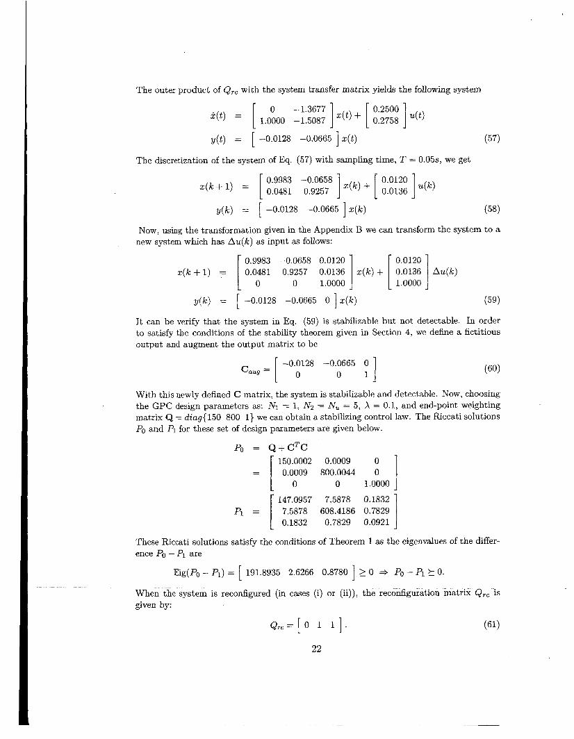
The outer product of QTC with the system transfer matrix yields the following system

i

k( t ) = [ O -1.3677] z ( t ) + [ 0.2500 ] u(t) 1.0000 -1.5087 0.2758

0.9983 -0.0658 0.0481 0.9257

(58)

z ( k + 1 ) =

y(k) = [ -0.0128 -0.0665 ] z ( k )

Now, using the transformation given in the Appendix B we can transform the system to a new system which has Au(k) as input as follows: [ 0.9:3 -0.0658 0.0120 0.0120

0 1.0000 ] [ l.oooo] z (k + 1) = 0.0481 0.9257 0.0136 z(k) + 0.0136 Au(k)

y(k) = [ -0.0128 -0.0665 0 ] z ( k ) (59)

It can be verify that the system in Eq. (59) is stabilizable but not detectable. In order to satisfy the conditions of the stability theorem given in Section 4, we defme a fictitious output and augment the output matrix to be

(60) 1 [ -0.00128 -0.0665 0 0 1 Caug =

With t h s newly defined C matrix, the system is stabilizable and detectable. Now, choosing the GPC design parameters as: Nl = 1, Nz = Nu = 5, X = 0.1, and end-point weighting matrix Q = diag(l50 800 l} we can obtain a stabilizing control law. The Riccati solutions Po and PI for these set of design parameters are given below.

Po = Q + C T C

0.0009 800.0044 0

= [ 0 0 1 .oooo O I

1 150.0002 0.0009

147.0957 7.5878 0.1832 4 = [ 7.5878 608.4186 0.7829

0.1832 0.7829 0.0921

These Riccati solutions satisfy the conditions of Theorem 1 as the eigenvalues of the differ- ence PO -9 are

Eig(P0 - PI) = [ 191.8935 2.6266 0.8780 ] 2 0 + PO -9 ?I 0. ~. .- ~ ~

When the system is reconfigured (in cases (i) or (ii)), the reconfiguration matrix Q,, is given by:

Q r c = [ 0 1 1 1 . (61)

22

y ( t ) = [ -0.0128 -0.0665 ] z(t) (57)

The discretization of the system of Eq. (57) with sampling time, T = 0.05s, we get

Then, from Eq. (53) the system transfer matrix after reconfiguration effectively becomes

-0.0234 -0.0234 -0.0345 -0.0345

(62)

0.0000 -1.3677 1.0000 -1.5087 X(t) =

y(t) = [ -0.0000 0.0313 ] x ( t )

Again, discretization of the system with sampling time, T = 0.05s, yields

-0.0011 -0.0011 -0.0017 -0.0017

(63)

0.9983 -0.0658 0.0481 0.9257 z(k+1) =

y(k) = [ -0.oooO 0.0313 ] ~ ( k )

Again, as before, using the transformation given in the Appendix B one can transform the above system to a new system with An(k) as input as follows:

A+)

(64)

1 0.9983 -0.0658 -0.0011 -0.0011 -0.0011 -0.0011

0.0481 0.9257 -0.0017 -0.0017 1 x(k) + [ yobg -0-r17 0 1.0000 0 0 0 1.0000 J 0 1.mm J

x ( k + l ) =

l o y(k) = [ -0.0000 0.0313 0 0 ] x ( k )

This system again is not detectable and one can define new fictitious output as before and define a new C matrix as

0 1.0000 0 0 0 1.0000 O I

[ -0.y 0.0313 0 tau, =

The modified system with this new C matrix is again controllable and observable. Now if we d e h e the new GPC parameters to be IVl = 1, N2 = Nu = 5, X = 0.1, and the end-point weighting matrix as Q = diag{ 130 200 1 l}, we obtain the following Riccati solutions which satisfy the stability condition of Theorem 1 as shown below:

Po = Q + C T C

1.0000 0 0 0 0 0 0 1.0000 : I = [

9 = [ 130.0000 -0.0000 0 -0.0000 200.0010 0

129.9835 0.2793 -0.0146 -0.0146 0.2793 171.7884 -0.0275 -0.0275

-0.0146 -0.0275 0.0909 0.0000 -0.0146 -0.0275 0.0000 0.0909

~ p~

Eig(P0 - PI) = [ 28.2154p0.0i% 0.9095 0.9mf-I 20% P F P l - E 0.- ~~~

Thus the conditions in the Theorem 1 are satisfied and the GPC control law (Eq. (26)) stabilizes the system.

23

Case (i): Consider the first of the two cases mentioned above. In this case, it is assumed that after system output (pitch rate) reaches its steady-state value of 1.15 deglsec the elevator input abruptly goes to zero (at t = 2 secs) (potentially this could be a result of possible failure) and system is reconfigured using Eq. (6).

Figure 7 shows the system response before and after reconfiguration. It can be seen that the system reaches a zero steady-state error within 2 seconds and when elevator input abruptly goes to zero at t = 2 secs, the output starts drifting from the desired value. At t = 2 sec reconfiguration takes place and ailerons take over and bring back the output back to the desired value rendering zero steady-state error. The input time histories are given in Fig. 6. As shown in the figure, the elevator deflection has abruptly dropped to zero after reaching an approximate steady-state value of -1.8 deg and at the same instant ailerons take over and bring the output back to the desired value. The ailerons reach the steady deflection of about -19 deg. The cost and tracking error plots are given in Figs. 8 and 9, respectively.

. , . , .. -10

-15

-20 2 4 6 8 10 12

. . ; r

._ - - _ _ - -

, ; .. -15 - I >' I .

, !.,I -20

2 4 6 8 10 12

Figure 6: The GPC control law

Figure 7: The Plant Output

24

Figure 8: The Cost Function

Figure 9: The PIant Output Error

Case (ii): In the second case, it is assumed that the elevator input freezes to some nonzero constant -6 deg before the system output (pitch rate) reaches its desired value (5.73 deg/sec). The simulation results for this case are shown in Figures 10-13. A s shown in Fig. 10, the elevator input freezes approximately at -6 deg when the system output has reached only 90% of its final value. At this time ailerons take over as a result of reconfig- uration and ailerons deflection reaches a steady-state value of approximately -21 deg as pitch rate reaches to desired value of 5.73 deg/sec. As seen in Fig. 11, overall tracking performance is very satisfactory without steady-state error. The performance function and tracking error time history is shown in Figs. 12 and .13, respectively.

Z-€h3n&€dhg.Remks -~ ~~ ~~~ ~ ________ -

This paper presented a comprehensive development of the basic GPC control architecture and derivation of control law for SISO as well as MIMO systems. For SISO systems, both

25

1

5 - E k a w - LenAd.rm

R@l Abmn 0 - __ - -.

r

Figure 11: The Plant Output

z-domain (i.e., polynomial-based) as well as state-space based control law development was given. Stability of GPC based on end-point constraints was presented as a basis for establishing stability of a novel recodigurable GPC control architecture. The stability conditions for reconfiguration scheme were presented. A numerical example consisting of longitudinal control of aircraft was presented to demonstrate the effectiveness of the proposed reconfiguration methodology.

8 Acknowledgements The second and third author acknowledge the financial support from NASA Ames Research Center, Moffett Field, CA, through Grant No. NAG2-1471 under the direction of Dr. Michael R. Lowry, Computational Sciences Division. ~ ~~ ~

~ ~

26

Figure 12: The Cost Function

Figure 13: The Plant Output Error

References [l] J. Richalet, A. Rault, J.L. Testud, and J. Papon: ‘Algorithmic Control of Industrial

Processes’. In 4th IFAC symposium on Identification and System Parameter Estima- tion. Tbilisi URSS, 1976.

[2] J. Richalet, A. Rault, J.L. Testud, and J. Papon: ‘Model Predictive Heuristic Control: Application to Industrial Processes’, Autornatica, 14(2):413-428, 1978.

[3] A. I. Propoi: ‘Use of LP Methods for Synthesizing Sampled-Data Automatic Systems’, Automn Remote Control, 24, 1963.

[4] V. Peterka: ‘Predictor-Based Self-Tuning Control,’ Autornatica, 20( 1):39-50, 1984. [5] B. E. Ydstie: ‘Extended Horizon Adaptive Control’, IN Proc. 9th IFAC World

[6] C. Greco, G. Menga, E. Mosca, and G. Zappa: ‘Performance Improvement of Self- tuning Controllers by Multi-Step Horizons: the MIJSMAR approach’, Autornatica,

~ - _ _ -~ -- . __ ___ -Congress, Budapest, H84: _ _ -~ ~

20~681-700, 1984.

27

[7] J. M. Lemos and E. Mosca: ‘A Multipredictor-based LQ Self-tuning Controller’, In IFAC Symposium on Identification and System Parameter Estimation, York, UK, 137- 141, 1985.

[8] J . Richalet, S. Abu el Ata-Doss, C. Arber, H.B. Kuntze, A, Jacubash, and W. Schill: ‘ Predictive Functional Control: Application to Fast and Accurate Robots,’ In Proc. 10th IFAC Congress, Munich, 1987.

[9] R. Soeterboek: ‘Predictive Control: A Unified Appraoch,’ Prentice Hall, 1992.

[lo] M Morari: ‘Advances in Model-based Predictive Control’, Chapter in Model-based Predictive Control: Multivaraible Control Technique of Choice in the 1990s?’, Oxford Univ. Press, 1994.

[ll] C. Mohtadi: ‘Advanced Self-tuning Algorithm’, PhD thesis Oxford Univ., U.K., 1986.

[12] D. W. Clarke and Scattolini: ‘Constrained Receding-horizon Predictive Control’, Proc.

[13] E. Mosca, J. M. Lemos, and J. Zhang: ‘Stabilizing 1/0 Receding Horizon Control,’

[14] K.R. Muske and J. Rawlings: ‘Model Predictive Control with Linear Models’, AICHE

[15] Ming Ding: ‘Neural Network-Based Predictive Control of Uncertain Systems,’ M.S.

IEE, 138(4),:347-354, July 1991.

IEEE Conf. in Decision and Control, 1990.

Journal, 39:262-287, 1993.

Thesis, Mechanical Engineering Dept., Kansas State University, 1998.

[16] D.W.Clarke, C.Mohtadi, and P.S.Tuffs: Generalized Predictive Control- Part I. The

[17] D.W.Clarke, C.Mohtadi, and P.S.Tuffs: Generalized Predictive Control- Part 11. Ex-

[18] Properties of Generalized Predictive Control, D.W.Clarke, C.Mohtadi, Automatica, 25(6), 1989.

[19] R.R.Bitmead, M.Gevers, V.Wertz, and K.Ogata: Adaptive Optimal Control: The Thinking Man’s GPC, Prentice Hall, Englewood Cliffs, New Jersey, 07632, 1990.

[20] H.Demircioglu and D.W.Clarke: Generalized predictive control with end-point state weighting, IEE Proceedings-D, Vol. 140, No.4, July 1993.

[21] C.L.Phillips and H.T.Nagle: Digital Control System Analysis and Design, Third Edi- tion, Prentice Hall, Saddle River, New Jersey 07458, 1995.

[22] E.Mosca: Optimal, Predictive and Adaptive Control, Prentice Hall, Englewood Cliffs, New Jersey, 07632, 1995.

[23] K.Ogata: Discrete-Time Control Systems, Second Edition, Prentice Haii, Engiewood Cliffs, New Jersey, 07632, 1995.

Basic Algorithm, Automatica, 23(2), 1987.

tensions and Interpretations, Automatica, 23(2), 1987.

[24] E.F.Camacho and C.Bordons: Model Predictive Control, Springer-Verlag London Lim-

[25] Jeffrey B.Burl: Linear Optimal Control: ‘HE and 3-1, Methods, Addison-Wesley, 1999. ~ ~ ~

~ ~~

ited,1999.

[26] B.L.Stenvens and F.L.Lewis: Aircraft Control and Simulation, John Wiley and Sons, INC. 1992.

28

[27] R.A.Hess and Y.C.Jmg: An Application of Generalized Predictive Control to Rotor- craft Terrain-Following Flight, IEEE Transaction on Systems, Man and Cybernetics, 19(5), 1989.

[28] E.F.Camacho: Constrained Generalized Predictive Control, IEEE ?tansaction on Au- tomatic Control, 38(2), 1993.

[29] J.A.Rossiter and B.Kouvaritakis: Constrained Stable Generalized Predictive Control, IEE Proceedings-D, 140(4), 1993.

[30] D.Q.M.ayne, J.B.Rawhgs, C.V.Ra0, and P.O.Scokaert: Constrained Model Predictive Control: Stability and Optimality, Automatica, 36, 789-814, 2000.

[31] J.A.Primbs and V.NevistiC: Feasibility and Stability of Constrained Finite Receding Horizon Control, Automatica, 36(7), 956-971, 2000.

[32] J.A.Primbs and V.Nevistid: Constrained Finite Receding Horizon Linear Quadratic Control, Proceedings of 36th Conference on Decision and Control, 1997.

[33] A. Jadbabaie, J.Primbs, and J.Hauser: Unconstrained Receding Horizon Control with No Terminal Cost, Proceedings of the American Control Conference, 2001.

29

Appendix

A Diophantine equation The Diophantine equation offers a convenient way to obtain a division of two polynomials and has the following form:

1 = Ej(q-')A(q-') + q-jFj(q-l) (A-1)

where A(4-l) = AA(q-l). The degrees of polynomials Ej and Fj are j - 1 and n,, respectively. This equation will be useful in writing predictions of future outputs. The Diophantine equation has a unique solution, Ej and Fj, given A(q-') and the prediction interval j.

Consider Eq. (2) and multiply it by EjAqJ to obtain

EjAA(q-')y(k + j ) = EjB(q-l)Au(k + j - d - 1) + Ej<(k + j ) ( A 4

Now substituting for EjAA from Eq. (A.l ) gives

y ( k + j ) = Fj(q- ' )y(k) + Ej(q-')B(q-l)Au(k + j - d - 1) + Ej (~ - l )<(k + j ) (A.3)

As the degree of polynomial EJ(q-l) = g - 1 the noise terms in Eq. (A.3) are all in the future and therefore can be omitted from the prediction as any better prediction of noise is not possible. The best prediction of y ( k + g) is therefore given by

Q(k +g) = G,(q- l )A~(k+g - d - 1) + FJ(q-l)y(k) (A.4)

where, G,(q-l) = EJ(q-l)B(q-l). Since the degrees of EJ and F3 are g - 1 and n,, the gth prediction of output involves the past outputs: ( y ( k ) , y ( k - l), .+ . , y(k - n,)) and inputs (Au(k + j - d - l), Au(k + 3 - d - 2), . . . , Au(k - d - nb)). The polynomials EJ and F3 obtained from Eq. (A.l ) are given by

EJ(q-l) = e,,o + e,,lq-' + . . . + eJ,J-lq-(J-l) FJ(4-l) = f3,o + f J , l ~ - ' + . . . + f j , n a ~ - ~ ~

Now, the same Diophantine equation can be used to obtain EJ+l and FJ+l, where

FJ+l(q-l) = f J + l , O + fJ+l,lQ-l+ . . . + fJ+l,naq-

EJ+l(q-') = EJ(Q-l) + eJ+l,Jq-J

G,+1 = EJ+lB = (E3 + f,,oq-J)B

and the polynomial E3+1 is be given by

.~ - ~~- with e,+l, = fJp. The polynomial ~ GJ+l can now be obtained recursively as follows

= GJ + fJ,OCJB (A.5)

30

where

Gj(Q-l) = gj,o + gj,lQ-’+ gj,2qV2 + . . . (A.6)

From Eqs. (A.5) and (A.6), it can be seen that the first j coefficients of Gj+l will be identical to those of Gj and the remaining ones are given by

g j+l j+ i = S j j+ i + f j , ~ h i = O , . . . , n b

In the case when system has a dead time of d, the output of the system at any time instant k is the result of input applied to the system at time k - d. As a result, the horizons N 1

and N2 should be chosen such that N2 2 N 1 2 d + 1. Now consider the following set of j-step ahead optimal predictions for j = d + 1, . . . , N 2 :

y^(k -/- d + 1) = Gd+lAu(k) + Fd+l?/(k)

y (k + d + 2) = Gd+zAu(k + 1) + Fd+2y(k)

y^(k + N2) = Gjv2Au(k + N2 - d - 1) + F ~ ~ y ( k )

which can be rewritten as:

3 = GAu + F(q-l)y(k) + G’(q-’)Au(k - 1)

where

Q(k + d + 1) Q(k + d + 2) I -

L y (k + N2)

Au(k) Au(k + 1)

A u = [ A u ( ~ +Nu - 1)

0 0

... 0 0 90 0 ...

0 E = SNI -d- 1 SNi -d-2 SN1 -d--3 . . ’

QN2-Nu-d L gNz-d-1 gN2-d-2 gN2-d-3 ...

and

QNi-d-1 gN1-d-2 " ' 0 QNi-d QN1-d-1 . ' . 0

QN2-d-1 QN2-d-2 ... QN2-Nu-d -

Thus, the predicted outputs over the prediction horizon are given by

where,

= G A u + f

w( t + ci + rvlj W = I w ( t + d + N1+ 1) ]

~ ( t + d + N2) ~ - _ _ _ _ ~ - ~ ~ - ~~

Equation (A.9) can be re-written as

1 2

J(N1, N2, Nu, A) = -AuTHAu + bAu + fo

32

Using Eq. (A.8), the cost function (Eq.(3)) can be written as

J ( N 1 , N2, Nu, A) = (GAu + f - w)*(GAu + f - w) + XAuTAu

where

w( t + ci + rvlj W = I w ( t + d + N1+ 1) ]

~- ~ ( t + d + N2)

- ~ _ _ _ _ ~ - ~ ~ _. ~~

Equation (A.9) can be re-written as

1 2

J(N1, N2, Nu, A) = -AuTHAu + bAu + fo

A u ( ~ - 1)

- (Ni -d- l ) ) q N i -d gN1 -d- 1 4 g14-1 - . . . -

91q-1 - . . . - QN2 - d - 1 4 -(Nz-d-l))qN2-d

32

(A.lO)

where

H = 2(GTG+XI) b = 2 ( f - ~ ) ~ G fo = ( f - w ) T ( f - w )

Minimizing cost function (3) to obtain optimd control is an unconstrained optimization problem as no other constraints axe considered on control input or plant output. The optimal input Au* is obtained by setting the gradient of J with respect to Au equal to zero. That is,

Au* = -H-'bT = (GTG + AI)-'GT(w - f ) (A.ll)

The actual control signal sent to the plant is

Au*(k) = IIAu* (A.12)

where, 11 = [l, 0, 0 , . . . ,O] is the 1 x Nu row vector. From Eq. (A.12) it can be seen that Au*(k) is the f i s t element of vector Au*.

33

B System transformation Typically, most of the system equations are available in the form with the input being u and not Au. However, the GPC control law developed in Eq. (26) is based on the system having input Au. This section is intended to provide the equations to transform the system with input u to a system with input Au.

Consider a MIMO LTI system with p inputs and q outputs.

q k + 1) = &(k) + Bu(k) y ( k ) = &(k) +Du(k) (B.13)

where input to the system is u and output is y. Let H(z) denote the transfer function from u(k) to y ( k ) . Then,

Y(z) = H(z)U(z)

where H(z) has a realization

H = [%] Now let T(z) be the transfer function from new input Au(k) to u(k), i. e.,

U(Z) = T(z)AU(Z)

where, T(z) is p x p transfer matrix and has the form:

Suppose T(z) has a realization

T = [*] = [*I and the state

(B.14)

(B.15)

xA(k) = u ( k - 1). '

Now, let HA(.) denotes the system with input Au(k), output y ( k ) , and having following &&+space descrintinn I I----.

~ ( k + 1) = Ax(k) + BAu(k) y ( k ) = Cx(k) +DAu(k)

Y(z) = H(z)T(z)AU(z) = Hn(z)AU(k)

34

where Ha ( z ) has realization

and the new state is

(B.16)

35

. -

C Proof of Lemma 1 We will use the principle of optimality to derive the optimal control law. The principle of optimality is well known and is stated below The Principle of Optimality: An optimal policy has the property that whatever the initial state and the initial decision are, the re- maining decisions must constitute an optimal policy with regard to the state resulting from the first decision.

In the context of our problem, the principle may be stated as follows:

If a closed-loop control u*(k) = f ( x ( k ) ) is optimal over the interval 0 5 k 5 N , it is

Let us define a set of various costs Fj as follows also optimal over any subinterval m 5 k 5 N , where 0 5 m 5 N .

FN = xT(k + N ) ( Q + CTC)x(k + N) Fj = xT(k + j)CTCx(k + j ) + XAuT(k + j)Au(k + j ) ( j = O , l , . . . , N - l )

Then, we an re-write the cost function, Eq. (22), as follows

JN = Fo + FI + . . . + F N - ~ + FN - xT(k)CTCx(k)

Note that x(k) does not affect the optimal control law Au*(j), for j 2 k .

Let S, (m = 1 , 2 , . . - , N + 1) be the cost from j = k + N - m + 1 to j = k + N . Then S, can be written as

From the Principle of Optimality if JN is the optimal cost, then so is S,. By the definition of Sm, we know that

Sm+l = sm+FN-m = S, + xT(k + N - m)CTCx(k + N - m) +

XAuT(k + N - m)Au(k + N - m) (C.17)

If 5'; is the optimal cost then we can get the optimal control Au*(k + N - m) by replacing S,,, by Sk in Eq. (C.17) and then setting

= O dSm+1 dAu(k + N - m)

(C.18)

We will obtain the expression for the optiniai cuntrol by the m c t h ~ d ef indl~ction Cnnsider SI. By the assumptions of GPC, Au(k + j ) = 0 for j 2 N . So

S; = xT(k + N ) ( Q + CTC)x(k + N ) _. = xT(k -k N ) F ( k + N)x(k -t N )

where is defined as

36

(C.191 . ~.

From Eq. (C.17): we get

S, = S ,*+FN-~ = S; + xT(k + N - l)CTCx(k + N - 1) + XAuT(k + N - l)Au(k + N - 1)

Substituting for S; and using state-space equation x(k + 1) = Ax(k) + BAu(k), we get

S2 = [ A x ( k + N - 1) + BAu(k + N - l)ITF(k + N)[Ax(k + N - 1) + BAu(k + N - l)] +x*(k + N - l)CTCx(k + N - 1) + XAuT(k + N - l)Au(k + N - 1)

Now setting

= O as2 dAu(k + N - 1)

we get optimal control law

Au*(k + N - 1) = - K ( k + N - l )x(k + N - 1)

where

K(k + N - 1) = [BT(Q + C*C)B + XI]-lBT(Q + CTC)A

and

s; = x T ( k + N - l ) x [(A - BK(k + N - l))T(Q + C T C ) ( A - BK(k + N - 1)) + CTC + XKT(k + N - l ) K ( k + N - l)] x x(k + N - 1) XT(k + N - l ) F ( k + N - l )x(k + N - 1) :=

F ( k + N - 1) is thus given by

P ( k + N - 1) = [(A - B K ( ~ + N - I > ) ~ ( Q + C ~ C ) ( A - B CTC + X K T ( k + N - l )K(k + N - l)]

From Eqs. (C.19) and (C.21), by induction we can write

: ( k + J

(C.20)

(C.21)

>I + ((2.22)

s; = X T ( k + N - m + l)F(k + N - m + l )x(k + N - m + 1)

and

Sm+l =

= S; + xT(k + N - m)CTCx(k + N - m) + XAuT(k + N - m>Au(k + N - m)

[Ax(k + N - m) +BAu(k + N - m)ITB(k + N - m+ 1) x

+xT_Lk + N - m)CTCx(k + N - m) + XAuT(k + N - m)Au(k + N - m)

[ A x ( k + N - m) + BAu(k + N - m)]

--------____--_____ ~ ~- __ ~ --___ - .__ __ __ - - - - .

Now, Eq. (C.18) can be used to find the optimal control law as follows

= 0 + Au*(k + N - m) = -K(k + N - m)x(k + N - m) (C.23) =*+1 aAu(k + N - m)

37

where

K(k + N - m) = [BTF(k + N - m + l)B + XI]-lBTp(k + N - m + l )A (C.24)

Substituting for AU yields

s;,, = x T ( k + N - m ) x

[(A - BK(~C + N - V L ) ) ~ F ( ~ + N - m + I)(A - B K ( ~ + N - m)) + CTC + XKT(k + N - m)K(k + N - m)] x

x(k + N - m) XT(k + N - m ) F ( k + N - m)x(lC + N - m) :=

where, F ( k + N - m) is given by

F ( k + N - m) = ATF(k + N - m + 1)(A - BK(k + N - m)) + CTC (C.25)

and the optimal cost is given by

s;v+l = xT(k)F(k)x(k) J; = S;vtl - xT(k)C%x(k)

= xT(k)(F(k) - CTC)x(k)

From Eqs. (C.20), (C.24) and (C.25), the optimal control law Au*(k) is given by

Au*(k) = -K(k)x(k) (C.26)

where, K ( k ) is obtained from the following recursive equation

K(k + j ) = [BTF(k + j + l)B -1 XI]-'BTF(k + j + l ) A (C.27)

and p ( k ) is the solution of the Riccati Difference Equation (RDE)

F(k+j) = AT~(k+j+1)A-ATF(k+j+l)B[BTF(k+j+1)B+XI]~1BTF(k+j+l)A+CTC (C.28)

with the boundary condition F ( k + N ) =Q+CTC (C.29)

38

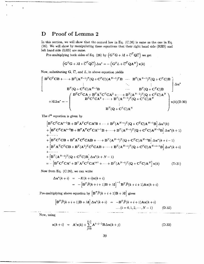
D Proof of Lemma 2 In this section, we will show that the control law in Eq. (C.26) is same as the one in Eq. (26). We will show by manipulating these equations that their right hand side (RHS) and left hand side (LHS) are same.

-T - Pre-multiplying both sides of Eq. (26) by (GTG + AI + C QC) we get

( G ~ G + XI + FQF) aU* = - (GTL + C ~ Q A N ) x(k)

NOW, substituting G, E, and L, in above equation yields

B ~ C ~ C B + . - - + B ~ ( A N - ~ ) T ( Q + cTc)(AN-~)TB . . . BT(AN-~)*(Q + CTC)B 1 Au*

I B ~ ( Q + c ~ c ) A ~ - ~ B ... BT(Q + CTC)B

x( k) (D.30)

B ~ C ~ C A + B ~ A ~ C ~ C A ~ + . . . + B ~ ( A ~ - ' ) ~ ( Q + C ~ C ) A ~ B ~ C ~ C A ~ + . . . + B ~ ( A ~ - ~ ) ~ ( Q + C ~ C ) A ~ i B'(Q + CTCjA"

+AIAu* = -

I The ith equation is given by

[BTCTCA'-lB + BTATCTCA'B + . . . + BT(AN-')T(Q + CTC)AN-'B] Au*(k)

+ [BTCTCA'-2B + BTATCTCA'-lB +.. . + BT(AN-*)T(Q + CTC)AN-2B] Au*(k + 1) +..-... + [BTCTCB + BTATCTCAB + ... + BT(AN-')T(Q + CTC)AN-'B] Au*(k + i - 1)

+ [BTATCTCB + BT(A2)TCTCAB +. . . + BT(AN-')T(Q + CTC)AN-'-'B] Au*(k + i) +......

+ [BT(A"-')T(Q + C*C)B] Au*(lc + N - 1)

= - [ B C T CA* + BTATCTCA'+' + . . . + BT(AN-')'(Q + CTC)AN] x(k) (D.31)

Now from w. (C.26), we can write

Au*(k + i) = -K(k + i)x(k + i) = - [BTB(k + i + l)B + AI]-' BTB(k + i + 1)Ax(k + i)

Pre-multiplying above equation by [BTF(k + i + l)B + XI] gives

[BT&k + i + l)B + AI] Au*(k + i) = -BT$(k + i + 1)Ax(k + i) . ._ (i = 0 , 1 , 2 , - . - , N - 1)

_ _ ~ -- -_ ~~~ ~ ~ - ___- ~

Now, using

2-1

x(k + i) = ~ * ~ ( k ) + A ~ - - ~ - ~ B A u ( ~ + j ) 3=0

(D.32)

(D.33)

39

we can write Eq. (D.32) as

A 4 k ) Au(k + I)

Au(k + i - 1)

Substituting for index i, we get

BTF(k + l)B BT$(k + 2)AB BT&k + 2)B

B T P ~ + N ) A ~ - ~ B ~ ~ ? ( k + N ) A ~ - ~ B . . . B ~ P ( ~ + N)B

(D.34)

Au*(k) Au*(k + 1)

Au*(k + N - 1) -. AU*

Note that Eqs. (D.30) and (D.35) have similar structure. Now, if we transform the RHS of Eq. (D.35) to match that of Eq. (D.30) and, as a result, if we get the LHS of both equations to match we have proved the lemma.

So, first transform the RHS of Eq. (D.35) to match that of Eq. (D.30). Consider the ith row in the RHS of Eq. (D.35). By Eq. (C.25), we have

P ( k + i) = =

A T P ( k + i + l )A + CTC - ATP(k + i + l)BK(k + i) AT[ATF(k + i + 2)A + CTC - A T F ( k + i + 2)BK(k + i + 1)]A + CTC - A T P ( k + i + l)BK(k + i)

and f2 = [BT(AN-i)Tp(k + N ) B K ( k + N - l)AN-l BT(AN-i-’)Tp(k + N - l )BK(k + N - 2)AN-’ - BTATp(k + i + l)BK(k + i )A i ]x (k )

(D.38) (D.39)

(D-40)

Note that, CP is same as the RHS of Eq. (D.31). Next, we will move f2 to the LHS, and then simplify the equation. Now, by (D.33), we have

i-1 AZx(k) = x(k + i) - AZ-j-’BAu(k + j ) (D.41)

(D.42)

Substituting Eq. (D.41) in R and using optimal control law, Au*(k+j) = -K(k+ j )x (k+ j ) , we get

j=O

R = - B ~ ( A ~ - * ) ~ P ( ~ + N)BAU*(~ + N - 1)

- B T ( A N - ~ ) T F ( ~ + N)BK(~ + N - 1) ( A N - ~ B A ~ ( ~ ) + . . . + B A U ( ~ + N - 2 ) )

-BT(AN-i-l)TP(k + N - 1)BAu*(k + N - 2)

-BT(A-v-i-l)TF(k + N - ljBK(k + N - 2 ) (A”-’BAu(k) + . - - + BAu(k + N - 3))

-BTATp(k + i + l)BAu*(k + i) - . . . . . .

-BTAT$(~ + i + I ) B K ( ~ + i) ( A ~ - ~ B A ~ ( ~ I + . . . + B A U ( ~ + i - 1))

The the ith row of LHS of Eq. (C.26) is

B ~ P ( ~ + ~ ) A ~ - ~ B A ~ * ( ~ ) + B V ( ~ + ~)A*-’BAu*(~ + 1) .. . + B ~ P ( ~ + ~ ) B A u * ( ~ + i - 1) (D.43)

Substituting Eq. (D.43) in Eq. (D.36) and moving f2 to the LHS, we get the coefficients of Au*(k) on LHS as

B ~ [ ( A ~ - Z ) ~ F ( ~ + N ) A ~ - ~ + (AN-i-~)TcTcAN-i-1 + . . . + CTC]Ai-’B

where, P(k + N) = CTC + Q. This coefficient is same as the one in Eq. (D.31). Similarly, we can relate the coefficients of Au*(k + j) (j = 1 , 2 , . . . , i - 1) to the ones in Eq. (D.31). Next, look at the coefficients of Au*(k + j ) , ( j = i, i + 1,. . . , N - 1). For j = N - 1, the coefficient of Au*(k+j)) on LHS becomes BT(AN- i )Tp(k+N)B, which is same as in Eq. (D.31). For j = i, the coefficient of Au*(k + j ) ) on LHS is given by

BTAT$(k + i + l)B + BT(A2)T@(k + i + 2 ) B K ( k + i + l ) B + . . . + B ~ ( A ~ - ~ - I ) V ( ~ + N - I ) B K ( ~ + N - ~ ) A ~ - ~ - ~ B

+ B ~ ( A ~ - ~ ) V ( ~ + N ) B K ( ~ + N - ~ ) A ~ - ’ - ~ B

n o m Eq. (D.36), we have

P ( k + i + 1)

-(AN-i-l)TF(k + N ) B K ( k + N - 1)AN-i-2 - ( A N - - ~ - ~ ) T F ( ~ + N - ~)BK(](: + N - 2 1 ~ ~ 4 - 3 - . . . -ATP(k + i + 2 ) B K ( k + i + 1)

- . -=~fffN-”-~~TP~ktN)AN,i-l-f tA“- i -~~~C-T€~ .N-a~~_~ ~_. -$- CTC ~

41

Substituting p ( k + i + I), we get the coefficient of Au*(k + i) as follows

BT(AN-i)Tp(k + N)AN-Z-lB + BT(AN-Z-l)TCTCAN-i-2B

+ . . . + B ~ A ~ C ~ C B

which is same as the one in Eq. (D.31).

given by Eq. (C.26) w Thus, we have shown that the optimal control law given by Eq. (26) is same as the one

Numerical Example:

Consider an LTI system,

x(k + 1) = Ax(k) + BAu(k)

Y(k) = Cx(k)

where

and the cost function of Eq. (22). Let the GPC control parameters be X = 1, N1 = 1, Nz = Nu = 3, and

Q = ill.

Now the GPC control law computed by Eq. (26) yields

-T - - I - Kgpc = (GTG + X I + C QC) (CQA3 + GTL) 3.6368 2.4684

0.1072 -0.3723

Similarly, the LQ control law computation for the same cost function using Eq. (D.35) yields

K l p T =

- -

B V ( ~ ) B + x BTp(2)AB BTp(2)B + X BTp(3)A2B BTp(3)AB BTp(3)B + X

3.6368 2.4684 1 1.8240 3.1017 0.1072 -0.3723

BTp(2)A2

which is same as Kgpc. This shows that both control laws are the same at time instant t = k.-When the cost- horizons for GPC and LQ strategies-ge identical.

42