Government Spending, Political Cycles and the Cross ... Belo... · Government Spending, Political Cycles and the ... Government Spending, Political Cycles, ... Raghuram Rajan, Tarun

Government Spending, Political Cycles and the

Cross-Section of Stock Returns∗

Frederico Belo†, Vito D. Gala‡ and Jun Li§

October 2011

Abstract

Using a novel measure of industry exposure to government spending, we document pre-dictable variation in cash flows and stock returns over political cycles. During Democraticpresidencies, firms with high government exposure experience higher cash flows and stockreturns, while the opposite pattern holds true during Republican presidencies. Business cy-cles, firm characteristics, and standard risk factors do not account for the pattern in returnsacross presidencies. An investment strategy that exploits the presidential cycle predictabilitygenerates abnormal returns as large as 6.9 percent per annum. Our results suggest marketunder reaction to predictable variation in the effect of government spending policies.

JEL Classification: D57, E6, G18, G12, H50Keywords: Asset Pricing, Government Spending, Political Cycles, Input-Output Analysis.

∗We thank Viral Acharya, Raj Aggarwal, Santiago Bazdresch, John Boyd, Michael Brandt, Lauren Cohen,Murray Frank, Bob Goldstein, Francisco Gomes, Joao Gomes, Annette Vissing-Jorgensen, Samuli Knupfer, IgorMakarov, Stijn Van Nieuwerburgh, Francisco Palomino, Dimitris Papanikolaou, Raghuram Rajan, Tarun Ramado-rai, Elias Rantapuska, Nikolai Roussanov, Stephen Schaefer, Johan Walden, Joel Waldfogel, Mungo Wilson, Moto-hiro Yogo, Jianfeng Yu, Lu Zhang, and Yinglei Zhang for helpful comments. We are especially grateful to FrancoisGourio for constructive comments which have improved the paper. Finally, we also thank seminar participantsat the Adam Smith Asset Pricing Conference, CEPR European Summer Symposium in Financial Markets, ChinaInternational Conference in Finance, European Finance Association, FIRS Conference, London Business School,Panagora Asset Management, University of Minnesota, and University of Nottingham for comments. The authorsgratefully acknowledge the financial support from a Dean’s Small Research Grant, London Business School and theCrowell Memorial Prize from Panagora Asset Management. All errors are our own.

†Assistant Professor, Department of Finance, University of Minnesota. e-mail: [email protected]‡Assistant Professor, Department of Finance, London Business School. e-mail: [email protected]§Department of Finance, University of Minnesota. e-mail: [email protected]

1

1 Introduction

This paper investigates the impact of political cycles through the government spending channel

on the cross-section of U.S. stock returns. According to a partisan view of political cycles as in

Alesina (1987), Republicans and Democrats differ in policies related to taxes, government spending

and social benefits. We focus on government spending, which represents on average about 20%

of annual U.S. gross domestic product. Most financial economists would agree that government

spending has an impact on expected firm cash flows. In addition, the uncertainty about the

impact of government policies may affect the rate at which future cash flows are discounted. We

investigate empirically the importance of these channels.

To identify the impact of presidential partisan cycles on asset prices through the government

spending channel, we compare the stock market performance of firms in industries with ex-ante

different exposure to government spending and investigate their relative performance over pres-

idential partisan cycles. If government spending has a significant impact on asset prices, it can

be identified by the differential performance of firms with heterogeneous government exposure,

ceteris paribus. Furthermore, if the presidential partisan cycle affects stock returns through the

government spending channel, it should be reflected in the differential performance of these firms

across the presidential cycle.

We construct a novel measure of industry exposure to government spending using detailed

industry level data from the NIPA input-output accounts. This measure is defined as the pro-

portion of each industry’s total output that is purchased directly by the government sector, as

well as indirectly through the chain of economic links across industries. We then investigate the

link between stock returns, fundamentals and government spending over the presidential partisan

cycle.

Our main empirical findings can be summarized as follows. While we find unconditionally

no significant difference in the average returns of firms with heterogenous government exposure,

we document a large and significant variation in average returns conditional on the presidential

partisan cycle. During Democratic presidential terms, firms in industries with high government

exposure significantly outperform firms in industries with low government exposure by about 6.1

2

percent per annum, but underperform by about 4.8 percent during Republican presidential terms.

This pattern holds even after controlling for firm-level characteristics, including market capitaliza-

tion, book-to-market, firm momentum, firm market beta and corporate political contributions, as

well as business cycle fluctuations. In addition, we show that the size of the presidential stock mar-

ket puzzle identified in Santa-Clara and Valkanov (2003) - i.e. average excess returns in the U.S.

aggregate stock market are substantially higher under Democratic than Republican presidencies -

is significantly more concentrated in industries with high exposure to government spending. The

difference in average excess returns across presidencies increases monotonically with the industry

exposure to government spending from 2.6 percent to 13.5 percent.

We also investigate whether the variation in average stock returns over the presidential partisan

cycle is due to differences in expected returns (risk premia) or abnormal returns. We construct an

investment strategy that exploits the presidential partisan cycle predictability in the cross-section

of stock returns and show that this strategy yields abnormal returns as large as 6.9 percent

per annum. Moreover, these returns are mainly concentrated during the second and third year

of the presidential term when political uncertainty about the winning party and its associated

government spending policy is more likely to have been resolved. These findings are robust to

different specifications of asset pricing models.

To understand the underlying economic channels driving the results we then investigate the

relationship between exposure to government spending and firms’ fundamentals over presidential

partisan cycles. Specifically, we test for the hypotheses that the political cycle has an heterogenous

impact on the performance of firms with different government exposure due to differential effects

on firms’ expected cash flow and/or cash flow volatility. According to the expected cash flow

hypothesis, firms with high government exposure have higher expected profitability than firms with

low government exposure during Democratic presidencies, consistent with their higher realized

returns, and vice-versa during Republican presidencies. According to the cash flow volatility

hypothesis, the profitability of firms with high government exposure is more uncertain than that

of firms with low government exposure during Democratic presidencies, and vice-versa during

Republican presidencies. This hypothesis is consistent with a risk-based interpretation in which

average returns reflect a compensation for differences in cash flow risk across presidencies. The

3

empirical evidence on the mean and volatility of firms’ profitability across presidential cycles, along

with the abnormal return analysis, are overall more supportive of expected cash flow effects rather

than cash flow volatility effects. Together with the evidence on abnormal returns, which build

up only gradually over the term of the presidency, these results suggest market under reaction to

predictable variation in government spending policies by the party in the presidency.

Relatively few papers have studied the relationship between government policies and asset

prices. Theoretical contributions include Pastor and Veronesi (2011a), Gomes, Michaelides, and

Polkovnichenko (2010), and Croce, Kung, Nguyen, and Schmid (2011); while empirical contri-

butions can be found in Santa-Clara and Valkanov (2003), Tavares and Valkanov (2003) and

Boutchkova, Doshi, Durnev, and Molchanov (2011). In this paper, we exploit a novel measure of

exposure to the government sector and the time-series variation in the cross-section of stock re-

turns to identify the impact of government spending policies over political cycles on stock returns.

More generally, our analysis also contributes to the literature on the effects of political cycles on

the macroeconomy (see Alesina, Roubini, and Cohen (1997), and Drazen (2000) for surveys).1

Our identification strategy also complements the literature in macroeconomics that studies

the effect of government spending on the real economy. The classic approach is to fit VARs

to macroeconomic data in order to identify government spending shocks as in Rotemberg and

Woodford (1992), Blanchard and Perotti (2002), and Ramey (2011). Alternative identification

strategies focus on periods of significant “exogenous” expansion in US defense spending as in

Ramey and Shapiro (1998).2 In a contemporaneous paper, Nekarda and Ramey (2011) use a

measure (similar to ours) of industry-specific shifts in government demand based on NIPA input-

output accounts to investigate the industry-level effects of government purchases. More recently,

Cohen, Coval, and Malloy (2011) use changes in congressional committee chairmanship as a source

of exogenous variation in state-level federal expenditures.

This paper is also related to a growing empirical literature investigating the impact of various

forms of political connectedness on firm value.3 We document that economic measures of political

connectedness such as a firm’s exposure to government spending affect the cross-section of stock

returns, thus complementing the findings in this literature. Finally, our empirical findings are

related to the empirical asset pricing literature investigating the effect of firm characteristics (see

4

Fama and French (2008) for a survey), industry characteristics (Hou and Robinson (2006), and

Gomes, Kogan, and Yogo (2009)), and demographic characteristics (DellaVigna and Pollet (2007))

on the cross-section of stock returns. Our work emphasizes the role of exposure to government

spending in predicting the cross section of stock returns across presidential cycles, and investigates

the risk-return properties of an equity investment strategy exploiting this presidential partisan

cycle predictability.

The paper proceeds as follows. Section 2 describes the data and the construction of the

variables used in our empirical analysis. Section 3 presents the main empirical results on the

relationship between firms’ exposure to government spending and average excess stock returns

across presidential partisan cycles. Section 4 investigates the relationship between exposure to

government spending and firms’ fundamentals across presidential partisan cycles, and discusses

the overall empirical findings. Section 5 concludes. Further details on the data description and

the construction of the measure of industry exposure to government spending are provided in the

Appendix.

2 Data

In this section, we describe the data used in the empirical analysis and explain the construction

of the measure of industry exposure to government spending. We then use this measure to form

government exposure portfolios. We also describe the properties of aggregate government spending

data across presidential partisan cycles.

2.1 Industry Exposure to Government Spending and Financial Data

We measure the industry exposure to government spending at the three-digit standard industry

classification (SIC) level using data from the Benchmark Input-Output Accounts released by Bu-

reau of Economic Analysis. This dataset is useful for our purposes because it provides highly

disaggregated industry level information about the flow of goods among industries and, more im-

portantly, the flow of goods from each industry to its final uses, such as government consumption,

government investment, private consumption and private investment. We identify the level of

5

industry exposure to government spending as the proportion of the industry’s total output being

purchased by the government sector (federal plus state and local) for final use. In computing

this ratio, the total amount of the industry output being purchased by the government sector

takes into account both direct and indirect effects. The direct effect measures the fact that one

additional dollar of goods purchased by the government sector in, for example, the agriculture

industry, directly represents one additional dollar of sales in that industry. However, in order

to generate this additional sale, the agriculture industry requires intermediate inputs from other

industries to produce its output, thus increasing demand (and hence output) in these industries

as well. The chain of input-output relationships among industries thus gives rise to an indirect

government spending effect, which we compute using the Leontief inverse, that is widely used

in standard Input-Output analysis (see ten Raa (2006)). Accounting for both effects provides a

comprehensive measure of each industry real exposure to government spending. Appendix A-1

provides a detailed explanation of the procedure.

The data from the Input-Output tables is available from 1947 to 2002, thus covering a relatively

large number of presidential terms. The Input-Output accounts are available for the years 1947,

1958, 1963, 1967 and, after 1967, all years ending with 2 and 7. To ensure that the investment

strategy in the following analysis is tradable - investors’ decisions are based only on information

publicly available at each point in time - we update the measure of industry exposure to government

spending when the new Input-Output table is released to the general public (the release dates of

each Input-Output table is obtained from the Bureau of Economic Analysis). The lag between the

collection of the data of each Input-Output table and its release to the general public is substantial.

For example, the first Input-Output table is for the year 1947, but the information from this table

only becomes publicly available in 1955. Therefore, the tradability requirement as well as the

availability of data on firms’ fundamentals (which we discuss below), restrict our sample to start

in July of 1955 and end in December 2009. Thus our main sample covers six Democratic and nine

Republican presidential terms. Whenever possible, we also investigate the robustness of our results

on a longer sample starting in 1929. Although there are no data on firms’ fundamentals available

over the entire extended sample, and the investment strategies are effectively not tradable prior

to 1955, the longer sample allows for the inclusion of seven additional presidential terms.

6

Monthly stock returns are from the Center for Research in Security Prices (CRSP) and firm

level accounting information is from the CRSP/COMPUSTAT Merged Annual Industrial Files.

To be included in our sample, a firm must have monthly stock returns, SIC code, and market

capitalization (size). In addition, as standard in the asset pricing literature, we remove firms in

the heavily regulated utility and financial sectors (SIC codes between 4900-4949 and 6000-6999,

respectively). We use the three-digit SIC code to identify an industry. We use COMPUSTAT

historical SIC codes, if not missing, because they are more accurate (see Kahle and Walkling

(1998)). If COMPUSTAT historical SIC code is missing, we use the corresponding CRSP SIC

codes. Appendix A-2 provides a detailed description of the CRSP and COMPUSTAT data and

sample selection criteria used in the empirical analysis.

Table 1 reports the summary statistics of the measure of industry exposure to government

spending. The average across all years is about 13.2 percent and its cross-sectional distribution

is fairly stable across Democratic and Republican presidencies. More than 90.0 percent of the

industries have sales to the government sector that represent less than 30.0 percent of the industry’s

total sales. Hence, the mass of the government exposure distribution is concentrated at low values,

which reflects the fact that most of the final demand in the U.S. economy is from the private sector

(private consumption and investment) rather than from the government sector. However, the high

values (max) of industry exposure to government spending also make clear that some industries

rely heavily on the government sector as a final consumer.

[Insert Table 1 Here]

Table 1 also reports the summary statistics of value-weighted aggregate stock market excess

returns across all years in the sample period, and across Democratic and Republican presidential

terms. It also reports the average number of firms included in the sample. The average aggregate

stock market excess return is considerably higher under Democratic than Republican presidencies,

15.3 percent and 7.7 percent per annum, respectively. This finding is consistent with the presiden-

tial stock market puzzle identified in Santa-Clara and Valkanov (2003), who also show that such

a large difference in average returns is robust to careful treatments of outliers and small sample

bias issues.

7

2.2 Government Spending Across Presidencies

To understand the impact of government spending policies over presidential partisan cycles on

stock returns, it is important to investigate the existence of systematic differences in government

spending during Democratic and Republican presidencies, and their relationship with the business

cycle. Table 2 reports the summary statistics of real per capita gross domestic product (GDP)

growth and total government spending growth (∆G). The summary statistics include means

and standard deviations across presidencies over the main (1955-2009), the extended (1929-2009),

and the post World War II (1947-2009) sample periods. The macroeconomic data is from the

National Income Product Accounts available through the Bureau of Economic Analysis website

(Table 1.1.6).


In the main sample period, government spending growth is on average higher under Democratic

than Republican presidential terms. The difference in the volatility of government spending across

presidencies is instead fairly small. However, both differences in mean and volatility of government

spending across presidencies are statistically insignificant at conventional levels, possibly because

of the relatively short sample size and the noisy aggregate government spending data.

To increase the statistical power, we also investigate these differences during the extended

sample from 1929 to 2009. The difference between the properties of government spending growth

across Democratic and Republican presidencies is more clear both in terms of mean (4.2 per-

cent versus 0.6 percent, respectively) and volatility (24.8 percent versus 3.2 percent, respectively).

While the difference in the average government spending across presidential terms is still sta-

tistically insignificant at conventional levels, uncertainty of government spending is significantly

higher under Democratic than Republican presidencies. Although this longer period might be less

representative being heavily influenced by the Great Depression and the large defense spending

during several war episodes including World War II, it still provides informative empirical evidence

of systematic differences in government spending policies across the presidential partisan cycle.

Interestingly, even in the post World War II sample (1947-2009), the total government spending

growth is on average higher during Democratic presidencies than during Republican presidencies

8

(3.5 percent versus 0.4 percent, respectively), and more volatile (6.6 percent versus 2.9 percent,

respectively), with both these differences being statistically significant at conventional levels. How-

ever, even this sample period is substantially influenced by the large defense spending during the

Korean war from 1950 to 1953. In unreported results, we show that the empirical analysis of this

section also holds for nondefense government spending.

Overall, the evidence in this section seems supportive of systematic differences in the govern-

ment spending policies across presidencies, with government spending growth being on average

higher and more volatile under Democratic than Republican presidential terms. Consistent with

the evidence in Alesina and Rosenthal (1995) and Alesina, Roubini, and Cohen (1997), annual

GDP growth is also on average significantly higher under Democratic than Republican presiden-

tial terms. However, this high correlation between the presidential partisan cycle and the business

cycle makes it particularly challenging to use directly aggregate government spending data to

identify the effect of the presidential cycle on stock returns through the government spending

channel. Hence, we focus on an indirect identification strategy which explores the differential per-

formance of publicly traded firms with ex-ante different exposure to government spending across

the presidential partisan cycles. Furthermore, according to a partisan view of political cycles, dif-

ferences in the government spending policies of Democrats and Republicans concern not only the

overall level of spending, but also its allocation across firms. While differences in the overall level

of spending, even if statistically challenging, can be investigated directly using macroeconomic

data, our indirect identification approach based on a large cross-section of firms is more suitable

to identify differences in the allocation of government expenditures across firms over presidential

cycles.

2.3 Government Exposure Portfolios

To investigate the relationship between exposure to government spending and stock returns, we

form five portfolios sorted on the level of industry exposure to government spending. We refer to

these portfolios as the government exposure portfolios.

This portfolio approach and sorting procedure is a convenient way to investigate our research

question. By construction, these portfolios maximize the spread in the industry exposure to gov-

9

ernment spending and thus differences in their average returns can be more accurately attributed

to differences in the sorting variable. The portfolio approach also reduces the impact on aver-

age returns of other industry effects. The sorting on an ex-ante measure of industry exposure to

government spending differs from the more conventional procedure of creating portfolios sorted

on pre-ranked government spending betas (e.g. Breeden, Gibbons, and Litzenberger (1989), and

Lamont (2001)) since it does not require any estimation. Thus, the cash-flows of the industries

in the portfolios are economically rather than just statistically linked to government spending. In

addition, the alternative approach based on the estimation of government spending betas requires

high frequency government spending data. However, the high level of aggregation and the poor

quality of the available government spending data, as well as the lack of information about the

separate expenditures on publicly traded firms, makes this approach less feasible in practice.

In constructing the five government exposure portfolios we follow the methodology in Fama

and French (1993). In each June of year t, we first sort the universe of common stocks into

five portfolios based on the industry exposure to government spending. The cutoffs used for the

portfolio formation are the quintiles of the industry exposure to government spending at the end

of year t−1. Once the portfolios are formed, their value-weighted returns are tracked from July of

year t to June of year t+1.4 The portfolios are re-balanced annually. Because of the updates in the

Input-Output Accounts (approximately every five years), some industries move across government

exposure portfolios. The transition frequencies are given in Table 3. Importantly, the government

exposure portfolios are very stable, and thus the investment strategies investigated in the following

sections are likely to have low turnover costs.5


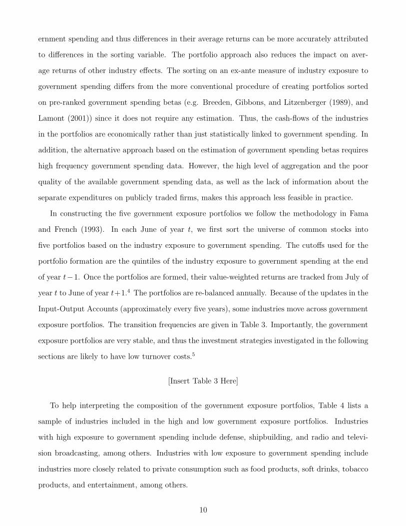
To help interpreting the composition of the government exposure portfolios, Table 4 lists a

sample of industries included in the high and low government exposure portfolios. Industries

with high exposure to government spending include defense, shipbuilding, and radio and televi-

sion broadcasting, among others. Industries with low exposure to government spending include

industries more closely related to private consumption such as food products, soft drinks, tobacco

products, and entertainment, among others.

10


Table 5 reports the summary statistics of selected firm characteristics of the five government

exposure portfolios across all years. Importantly, the spread in the level of exposure to government

spending across the extreme portfolios is high, with the difference being more modest across the

intermediate portfolios. The average industry exposure to government spending of the low and high

government portfolios is around 1.5% and 29.6%, respectively. This large spread contributes to

validate our identification strategy as, if any, the larger the spread, the larger the differential impact

on firms’ performance of changes in government spending, ceteris paribus. For the intermediate

portfolios, the difference ranges from 4.8% (portfolio 2) to 14.7% (portfolio 4). Each government

portfolio represents on average an approximately equal number of industries, which mitigates

concerns that our results may be driven by few industries only. For instance, in unreported results,

we find that excluding firms in the defense sector (including Fama-French industry classification

24 (Aircraft), 25 (Ships), and 26 (Defense)) does not affect the main empirical findings. While

portfolios with low government exposure tend to have relatively higher book-to-market ratios and

leverage, there are no significant differences in firm size across the government exposure portfolios.


3 Government Spending Exposure and the Cross-Section

of Stock Returns

In this section we establish our main empirical findings. Conditional on the presidential partisan

cycle, firms’ exposure to government spending predicts the cross-section of stock returns. The

predictability holds even after controlling for other firm characteristics known to predict stock

returns, for business cycle effects and for time-varying risk measures, and it is stronger among

firms’ located in U.S. states that benefit the most from federal spending.

11

3.1 Returns of the Government Exposure Portfolios

Table 6 shows the average annual excess returns of the government exposure portfolios across

all years (654 months), Republican presidential terms (403 months) and Democratic presidential

terms (251 months). We focus our analysis on the main tradable sample period from 1955 to 2009.

We also investigate the results on the extended (though non-tradable prior to 1955) sample period

from 1929 to 2009 for robustness.


The top panel in Table 6 shows that, across all years during the tradable period 1955-2009, the

average excess returns of the government exposure portfolios are not significantly different, with

a difference of only −0.6 percent between the high and low government exposure portfolios. Our

main empirical finding follows from the analysis of the average portfolio returns across presidential

terms. During Democratic presidential terms, the high government exposure portfolio outperforms

the low government exposure portfolio by 6.1 percent, and this difference is statistically significant

at conventional levels. The sign of the spread in returns is reversed during Republican presidential

terms: the high government exposure portfolio significantly underperforms the low government

exposure portfolio by 4.8 percent.

The pattern in average excess returns reported in Table 6 also shows that the presidential stock

market puzzle identified in Santa-Clara and Valkanov (2003) is significantly more concentrated

in industries with high exposure to government spending than in industries with low exposure.

The difference in the average performance of the high government exposure portfolio between

Democratic and Republican presidential terms is large and significant, 14.9 percent versus 1.4

percent, respectively. For the low government exposure portfolio, this difference is small and

statistically insignificant, 8.7 percent versus 6.1 percent, respectively. More generally, the difference

in the average realized returns of the government portfolios across presidential terms increases

monotonically with the industry exposure to government spending. These empirical findings

suggest that government spending is a plausible economic channel through which the party in the

presidency can affect stock returns.

12

The main sample from 1955 to 2009 covers fifteen presidential terms. To investigate the

robustness of our findings, we extend the sample backwards to start in 1929, corresponding to the

beginning of the mandate of the first president (Hoover) in the CRSP database. In the absence

of Input-Output tables covering this earlier period, and considering that the distribution of the

government exposure variable is fairly stable over time (as documented in Table 3), we assign the

industry exposure to government spending in 1955 to all years prior to 1955. While our portfolios

are effectively not tradable prior to 1955, this extension allows the inclusion of seven additional

presidencies: two Republican and five Democratic presidencies.

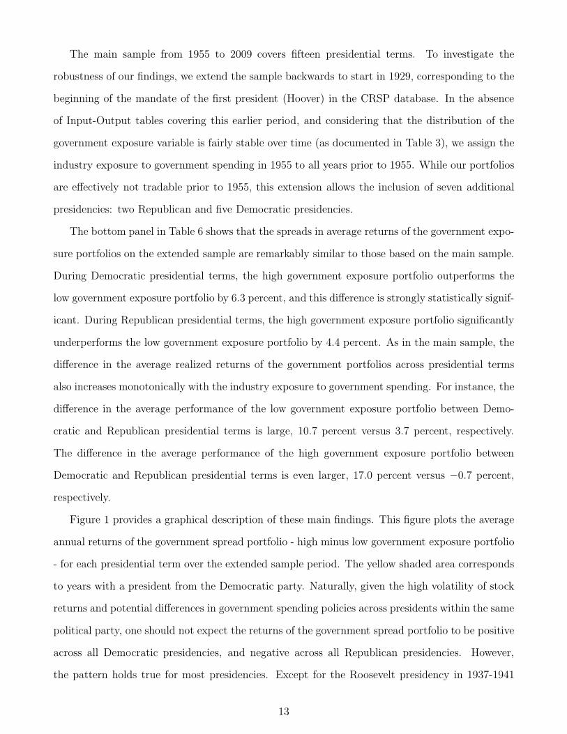
The bottom panel in Table 6 shows that the spreads in average returns of the government expo-

sure portfolios on the extended sample are remarkably similar to those based on the main sample.

During Democratic presidential terms, the high government exposure portfolio outperforms the

low government exposure portfolio by 6.3 percent, and this difference is strongly statistically signif-

icant. During Republican presidential terms, the high government exposure portfolio significantly

underperforms the low government exposure portfolio by 4.4 percent. As in the main sample, the

difference in the average realized returns of the government portfolios across presidential terms

also increases monotonically with the industry exposure to government spending. For instance, the

difference in the average performance of the low government exposure portfolio between Demo-

cratic and Republican presidential terms is large, 10.7 percent versus 3.7 percent, respectively.

The difference in the average performance of the high government exposure portfolio between

Democratic and Republican presidential terms is even larger, 17.0 percent versus −0.7 percent,

respectively.

Figure 1 provides a graphical description of these main findings. This figure plots the average

annual returns of the government spread portfolio - high minus low government exposure portfolio

- for each presidential term over the extended sample period. The yellow shaded area corresponds

to years with a president from the Democratic party. Naturally, given the high volatility of stock

returns and potential differences in government spending policies across presidents within the same

political party, one should not expect the returns of the government spread portfolio to be positive

across all Democratic presidencies, and negative across all Republican presidencies. However,

the pattern holds true for most presidencies. Except for the Roosevelt presidency in 1937-1941

13

and the Kennedy/Johnson presidency in 1961-1965, the high government portfolio significantly

outperforms the low government portfolio during most Democratic presidencies. For example,

during the first Roosevelt presidency in 1933-1937, the Carter presidency in 1977-1981 and Clinton

presidency 1993-1997, the high minus low government portfolio average annual returns are greater

than 10.0 percent. The pattern of average returns across Republican presidential terms is equally

impressive, except for the Eisenhower presidency in 1953-1957. The average return of the spread

portfolio is negative in seven out of the ten Republican presidential terms, consistently with the

summary statistics in Table 6.

[Insert Figure 1 Here]

3.2 Government Exposure and Geographical Location

The allocation of government expenditures in the economy may vary not only across industries,

but also across U.S. states. To the extent that the cross-sectional variation in returns across

presidencies is driven by differences in government spending policies, we should identify such

variation not only across industries, but also across firms’ geographical location. In particular,

if differences in government spending is indeed the underlying source of the differential cross-

sectional performance across presidencies, the effects should be stronger among firms located in

U.S. states that benefit disproportionately from federal spending.

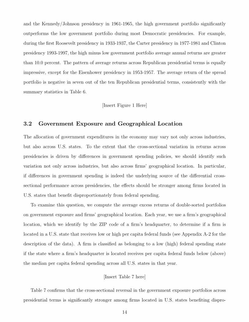
To examine this question, we compute the average excess returns of double-sorted portfolios

on government exposure and firms’ geographical location. Each year, we use a firm’s geographical

location, which we identify by the ZIP code of a firm’s headquarter, to determine if a firm is

located in a U.S. state that receives low or high per capita federal funds (see Appendix A-2 for the

description of the data). A firm is classified as belonging to a low (high) federal spending state

if the state where a firm’s headquarter is located receives per capita federal funds below (above)

the median per capita federal spending across all U.S. states in that year.

[Insert Table 7 here]

Table 7 confirms that the cross-sectional reversal in the government exposure portfolios across

presidential terms is significantly stronger among firms located in U.S. states benefiting dispro-

14

portionately from federal spending. During Democratic presidential terms in the 1955 − 2009

sample period, the high government exposure portfolio outperforms the low government exposure

portfolio by 5.9 percent in low federal spending states, and by a significant 7.0 percent in high

federal spending states. The sign of the spread in returns is reversed during Republican presiden-

tial terms: the high government exposure portfolio underperforms the low government exposure

portfolio by 1.6 percent in low federal spending states, and by a significant 7.7 percent in high

federal spending states.

The pattern in average excess returns reported in Table 7 also shows that the presidential stock

market puzzle is significantly more concentrated among firms with high exposure to government

spending headquartered in high federal spending states. The difference in the average perfor-

mance of the high minus low government exposure portfolio between Democratic and Republican

presidential terms is large and significant: 7.5 percent in low federal spending states versus 14.6

percent in high federal spending states.

3.3 Government Exposure and Firm Characteristics

The previous analysis provides preliminary evidence on the predictability of the cross-section of

stock returns across presidential terms by the government exposure variable. However, government

exposure might be correlated with other firm characteristics known to predict returns in the

cross-section. To identify the marginal predictive power of the government exposure variable,

we run standard Fama and MacBeth (1973) regressions of firm-level monthly stock returns on

firms’ exposure to government spending interacted with president dummies and other firm-level

characteristics.6

Table 8 reports the results for five different empirical specifications. In the first specification

(row 1) we include a constant, the industry exposure to government spending interacted with a

Democratic president dummy, and the industry exposure to government spending interacted with

a Republican president dummy. In the second specification (row 2), we control for other well-

known stock return predictors: firm market capitalization (size), book-to-market ratio (B/M),

momentum (mom), and firm-level time-varying beta computed from daily returns within each

month (Lewellen and Nagel (2006)). In the third specification (row 3), we also include a firm-level

15

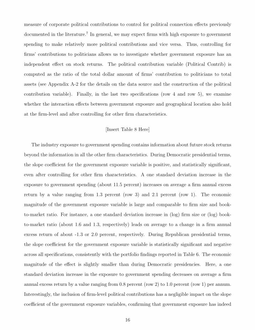
measure of corporate political contributions to control for political connection effects previously

documented in the literature.7 In general, we may expect firms with high exposure to government

spending to make relatively more political contributions and vice versa. Thus, controlling for

firms’ contributions to politicians allows us to investigate whether government exposure has an

independent effect on stock returns. The political contribution variable (Political Contrib) is

computed as the ratio of the total dollar amount of firms’ contribution to politicians to total

assets (see Appendix A-2 for the details on the data source and the construction of the political

contribution variable). Finally, in the last two specifications (row 4 and row 5), we examine

whether the interaction effects between government exposure and geographical location also hold

at the firm-level and after controlling for other firm characteristics.


The industry exposure to government spending contains information about future stock returns

beyond the information in all the other firm characteristics. During Democratic presidential terms,

the slope coefficient for the government exposure variable is positive, and statistically significant,

even after controlling for other firm characteristics. A one standard deviation increase in the

exposure to government spending (about 11.5 percent) increases on average a firm annual excess

return by a value ranging from 1.3 percent (row 3) and 2.1 percent (row 1). The economic

magnitude of the government exposure variable is large and comparable to firm size and book-

to-market ratio. For instance, a one standard deviation increase in (log) firm size or (log) book-

to-market ratio (about 1.6 and 1.3, respectively) leads on average to a change in a firm annual

excess return of about -1.3 or 2.0 percent, respectively. During Republican presidential terms,

the slope coefficient for the government exposure variable is statistically significant and negative

across all specifications, consistently with the portfolio findings reported in Table 6. The economic

magnitude of the effect is slightly smaller than during Democratic presidencies. Here, a one

standard deviation increase in the exposure to government spending decreases on average a firm

annual excess return by a value ranging from 0.8 percent (row 2) to 1.0 percent (row 1) per annum.

Interestingly, the inclusion of firm-level political contributions has a negligible impact on the slope

coefficient of the government exposure variables, confirming that government exposure has indeed

16

an independent effect on stock returns.

Finally, consistent with the portfolio level analysis reported in Table 7, the last two rows in

Table 8 show that the positive relationship between government exposure and stock returns during

Democratic presidencies is stronger among states with high dependence from federal spending

(Fed). Similarly, the negative relationship between government exposure and stock returns during

Republican presidencies is stronger among states with high dependence of federal spending, even

after controlling for other firm characteristics.

3.4 Government Exposure and Business Cycles

Since variations in returns have been associated with business cycle fluctuations and business

cycle fluctuations have been associated with political variables, the heterogenous impact of the

presidential partisan cycle on the government exposure portfolios might simply be due to business

cycle fluctuations. In fact, it is well known that Republican presidencies are associated with more

severe recessions, while Democratic presidencies are associated with more expansions, consistently

with the summary statistics in Table 2.8 Thus, different return sensitivities to the business cycle

of the government exposure portfolios might explain the pattern observed in the data.

To distinguish the political cycle from the business cycle effect on stock returns, we run time-

series portfolio returns predictability regressions of the form:

Rit+1 = β0i ·Demt + β1i · Rept + γ′

iXt + uit+1 , i = 1, .., 5 (1)

where Rit+1 is the ith government exposure portfolio monthly excess return, Demt and Rept are

political dummy variables equal to one if the beginning of the month president is from the Demo-

cratic or Republican party, respectively, and Xt is a vector containing lagged monthly business

cycle variables. Following the time-series predictability literature, we include the dividend yield

(DIV), the default spread (DEF), the term spread (TERM), and the short-term Treasury bill

rate (TB). We also include a set of macroeconomic business cycles variables, which are available

at monthly frequency and are not based on financial prices data, such as the inflation rate, the

unemployment rate and the growth rate in industrial production (IP).9 Appendix A-2 provides a

17

detailed description and data sources of these variables.


Table 9 reports the stock return predictability regression results for the five government expo-

sure portfolios, as well as for the government exposure spread portfolio (Hi-Lo). Controlling for

the business cycle variables has virtually no impact on the magnitude of the average excess returns

of the government exposure spread portfolio reported in Table 6. During Democratic presidential

terms, firms with high exposure to government spending significantly outperform firms with low

government exposure by 6.4 percent, but underperform during Republican presidential terms by

4.9 percent. In addition, the slope coefficients associated with the Democratic president dummy

increase almost monotonically with exposure to government spending, and the opposite pattern

is observed for the Republican president dummy slope coefficients. Table 9 also reports the differ-

ence in the slope coefficient of the Democratic and Republican dummies (Dif) to investigate the

differential impact of the presidential stock market puzzle identified in Santa-Clara and Valkanov

(2003) across government exposure portfolios. Consistent with the analysis in Table 6, the pres-

idential stock market puzzle is significantly more concentrated in industries with high exposure

to government spending than in industries with low exposure (19.7 percent versus 8.4 percent,

respectively), even after controlling for business cycle effects. Thus the heterogeneous impact of

the presidential partisan cycle on the returns of the government exposure portfolios is not driven

by business cycle fluctuations.

3.5 Expected or Abnormal Returns?

The previous analysis documents differences in the realized excess returns of the government expo-

sure portfolios across Democratic and Republican presidential terms, with these differences being

considerably larger in industries with high exposure to government spending. In this section, we

investigate whether the observed pattern in realized returns of the government exposure portfo-

lios across presidential terms can be attributed to variation in expected returns (risk-premia) or

abnormal returns. Differences in expected returns would be consistent with a risk story requir-

ing firms with high government exposure to be riskier than firms with low government exposure

18

during Democratic presidencies, with the reverse being true during Republican presidencies. In

contrast, if the pattern in the returns of the government portfolios across presidencies is due to

abnormal returns, it would suggest that the market is systematically surprised by the partisan

policies concerning government spending. In other words, abnormal returns would occur when

the government spending policies enacted by the party in the presidency deviate systematically

from what the market anticipates. To address this question, we now impose the structure of a

multifactor asset pricing model to formally control for risk and test for the presence of abnormal

returns in the government exposure portfolios across presidential terms.

3.5.1 Return Decomposition

The unconditional average returns of the government exposure spread portfolio (Hi-Lo) over the

entire sample period is close to and statistically indistinguishable from zero, but it is large and

significant once we condition on the presidential partisan cycle. Thus, we focus our analysis on

the risk and return properties of a political cycle investment strategy that captures the pattern

in returns of the government exposure portfolios across presidential partisan cycles in a simple

manner. We consider the following long-short investment strategy. During Democratic presiden-

cies, the strategy is long on the portfolio of firms with high government exposure and short on the

portfolio of firms with low government exposure, and during Republican presidencies, the long and

short positions are reversed. We define the average excess returns of this political cycle investment

strategy as the presidential investment premium.

Our analysis follows closely Ferson and Harvey (1999). To identify abnormal returns, we

assume a model of conditional expected returns that allows for time-variation in the quantity and

price of risk:

ERt = α +∑

i

βitλit (2)

βit = bi0 + b′

i1Zt (3)

where ERt is the conditional expected return of the political cycle investment strategy at time-t,

Zt is a vector of conditioning variables known at time t, βit is the conditional portfolio loading on

19

the risk factor i, λit = Et[Rit+1] is the conditional price of risk associated with the risk factor i,

and Rit+1 is the excess return of the risk factor i. Following the work of Fama and French (1993)

and Carhart (1997), we consider different combinations of standard risk factors including the stock

market, SMB, HML, and momentum. By allowing for several risk factors, we maximize the ability

of the asset pricing model to explain the time-series variation in the conditional expected returns

of the political cycle investment strategy, thus minimizing the likelihood that omitted risk factors

might be responsible for our findings.

Given the model of expected returns in equation (2), we test for abnormal returns by estimating

the following regression:

Rt+1 = α +∑

i

βit × Rit+1 + ǫt+1, (4)

where Rt+1 is the one-month ahead return of the political cycle investment strategy and βit is given

by equation (3). If the average returns of the political cycle investment strategy are explained by

exposure to standard risk factors, then the intercept α in (4) should be zero.

Table 10 reports the alphas from monthly time-series regressions of equation (4) for conditional

versions of the CAPM, the Fama and French (1993) three-factor model and the Carhart (1997)

four-factor model. In addition, for each asset pricing model, we report three alphas (α1, α2 and

α3), each obtained from an alternative specification of the set of instruments (Zt) included in

equation (3):

1. α1 : Zt = []. With no instruments, this specification corresponds to an unconditional asset

pricing model.

2. α2 : Zt = [DIV, DEF, TERM, TB]. This is the standard specification used in the empirical

asset pricing literature, which allows for time-varying risk.

3. α3 : Zt = [DIV, DEF, TERM, TB, DEM], where DEM is a Democratic dummy variable

which is equal to one if the president is from the Democratic party. This specification offers

a more flexible representation of conditioning information since it allows risk to vary over

time not only with business cycles but also with the presidential partisan cycles.

20

3.5.2 Abnormal Returns

Row 1 in Table 10 reports the average excess returns, the Sharpe ratio and the abnormal returns

of the political cycle investment strategy across alternative asset pricing models and conditioning

information sets. The presidential investment premium is large: the annual average excess return

of the political cycle investment strategy is about 5.3% per annum, with an annual Sharpe ratio

of 0.4. These values are statistically and economically significant. To put into perspective, the

presidential investment premium is about as large as the well-known value premium (Fama and

French (1992)), which is about 5.6% per annum.

In all asset pricing model specifications, we can reject at conventional levels the hypothesis that

the abnormal returns of the political cycle investment strategy are zero. For the unconditional

versions of the asset pricing models (α1), the abnormal returns of the strategy range from 3.3%

in the Carhart (1997) model to 5.6% in the Fama and French (1993) model. Allowing for risk to

vary over time with business cycles (α2) increases the magnitude of the abnormal returns of the

investment strategy across all asset pricing models. Here, the abnormal return range from 5.1% in

the Carhart (1997) model to 6.9% in the Fama and French (1993) model. Finally, allowing for risk

to vary over time also with presidential partisan cycles (α3) decreases significantly the abnormal

returns relative to the business cycle-only time-varying specification (α2). While the inclusion of

the presidential dummy in the set of conditioning instruments helps picking up time-variation in

risk associated with presidential partisan cycles, it does not explain the average returns of the

investment strategy. Across all models, the abnormal returns α3 are still statistically significant

and exceed 3.9% per annum.


3.5.3 Abnormal Returns Within Presidencies

The previous analysis shows that the presidential investment premium cannot be explained by

exposure to standard risk factors. However, there might be a latent political risk factor that

correlates with the presidential cycle and affects the returns on the presidential investment strategy.

If the presidential investment premium was indeed due to a higher (lower) ex-ante risk premium

21

across Democratic (Republican) presidencies, we should observe large movements in stock prices

earlier on during the term of the presidency when political uncertainty about the winning party and

its associated government spending policy is more likely to be resolved. In this section, we extend

the previous analysis to investigate the differences in realized and abnormal returns of the political

cycle investment strategy within presidential terms. Since each presidential term is composed of

four years, we examine the returns of the investment strategy separately across the first year of

the presidential term (Year 1), the second year (Year 2), the third year (Year 3) and the fourth

-election- year (Year 4). To obtain the abnormal return in each year of the presidential term, we

specify the alpha in equation (4) to be time-varying according to the following specification:

αt =

4∑

i=1

ai × Y ear(i)

where Y ear(i) is a dummy variable equal to one if the year of the presidential term is i and zero

otherwise.

Rows 2 to 5 in Table 10 show that the large presidential investment premium is significantly

more concentrated in the middle of the presidential term. The average excess returns of the

strategy are about 8.3% per annum in Year 2 and 7.2% per annum in Year 3, with corresponding

Sharpe ratios of 0.72 and 0.62, respectively. The pattern of abnormal returns within presidencies

mimics closely the pattern of the average excess returns of the investment strategy. During Year

2, the abnormal returns are strongly statistically significant across all model specifications and

exceed 6.9% per annum. Similarly, during Year 3, abnormal returns are large and in excess of

3.8% per annum. Differently, the average realized and abnormal returns of the investment strategy

during Year 1 and 4 are largely statistically insignificant.

Hence, we find no significant evidence of large realized returns concentrated earlier on during

the term of the presidency when political uncertainty about government spending policies is more

likely to be resolved. To the contrary, realized returns build up gradually over the term of the

presidency and tend to disappear towards its end.

22

4 Understanding Government Exposure Returns Across

Presidencies

The previous analysis documents a statistically reliable and economically meaningful link between

exposure to government spending and average stock returns across presidential partisan cycles.

Moreover, business cycle effects, firm characteristics, and exposure to standard risk factors do

not account for the cross-sectional pattern in returns across presidencies. In this section, we

investigate the relationship between exposure to government spending and firms’ fundamentals

across presidential partisan cycles to better understand the underlying economic links potentially

driving these empirical findings. Specifically, we focus our analysis on the following plausible

economic channels.

Hypothesis 1 (expected cash flow effect): During Democratic presidencies, high government

exposure firms earn higher stock returns because government spending under Democrats is higher

(relative to private spending) than under Republicans.

According to hypothesis 1, if a firm economically benefits by its exposure to government spend-

ing during Democratic presidencies, then these benefits should be reflected in terms of increases

in firm fundamental performance, such as increases in profitability. Similarly, if a firm suffers by

its exposure to government spending during Republican presidencies, then these economic losses

should be reflected in its profitability.

Hypothesis 2 (cash flow volatility effect): During Democratic presidencies, high government

exposure firms earn higher stock returns as compensation for the higher government spending

uncertainty (relative to private spending) under Democrats than under Republicans.

According to hypothesis 2, if government spending is more uncertain during Democratic presi-

dencies, then this uncertainty should be reflected in higher volatility of profitability for firms with

high government exposure. If this uncertainty is priced, then high exposure firms should earn

higher stock returns during Democratic presidential terms. Likewise, if government spending is

less uncertain during Republican presidencies, and this generates low uncertainty of the profitabil-

ity of high government exposure firms, then these firms should earn lower stock returns during

23

Republican presidential terms.

These hypothesis follow naturally from the previous empirical analysis, and they are not mutu-

ally exclusive as government spending can be simultaneously higher on average and more volatile

during Democratic presidencies. Indeed, these hypothesis are consistent with the overall properties

of aggregate government spending growth reported in Table 2, whereby the mean and volatility

(uncertainty) of government spending growth tends to be higher during Democratic presidencies.

Moreover, the expected return analysis in the previous section, which should in principle reflect

also cash flow uncertainty effects, already shows that the cross-sectional pattern in returns across

presidencies cannot be explained by exposure to standard risk factors. However, to the extent

that we might be omitting true unobservable risk factors, the direct investigation of cash flow

uncertainty effects can be informative about a risk-based explanation. In this section, we test

these two hypothesis using firm-level accounting data.

4.1 Expected Profitability Across Presidencies

To examine hypothesis 1 and quantify the relationship between the government exposure variable

and expected profitability, we estimate yearly Fama and MacBeth (1973) cross-sectional regressions

of firm-level annual return on equity (ROE), where ROE is equal to net earnings scaled by the book

value of equity, on lagged exposure to government spending interacted with president dummies,

and other firm-level characteristics. In the most general form, we estimate the following cross-

sectional regression:

ROEit+1 = α0+α1

Vit

Ait

+α2DDit+α3

Dit

Bit−1

+a4ROEit+α5Govit×Demt+α6Govit×Rept+εit+1. (5)

Panel A in Table 11 reports the results for three different empirical specifications. In the first

specification (row 1), we include only a constant, the industry exposure to government spending

(Gov) interacted with a Democratic president dummy (Dem), and the industry exposure to govern-

ment spending interacted with a Republican president dummy (Rep). In the second specification

(row 2), we control for other characteristics well known to predict future profitability such as the

ratio of market value of assets to book assets (V/A), a dummy variable for nondividend-paying

24

firms (DD) and the ratio of dividend payments to book equity (D/B). In the third specification

(row 3), we also control for lagged ROE to account for persistence in profitability. The inclusion

of these variables follows from the work by Fama and French (2000), Vuolteenaho (2002) and Hou

and Robinson (2006).


The results show that there is a positive relationship between firms’ future profitability and ex-

posure to government spending during Democratic presidential terms, and a negative relationship

during Republican presidential terms. Thus, consistent with hypothesis 1, firms more exposed to

government spending during Democratic years have higher expected profitability, and the reverse

holds true during Republican presidential terms. The estimated effects are economically large.

A one standard deviation increase in the exposure to government spending (about 11.5 percent)

increases on average a firm annual profitability by a value ranging from 0.5 percent (row 1) and 1.0

percent (row 2) during Democratic years. The effect on profitability is reversed during Republican

years: a one standard deviation increase in the exposure to government spending decreases on

average a firm annual profitability by a value ranging from 0.5 percent (row 3) and 0.9 percent

(row 1). The coefficients on the control variables (row 2) including a proxy for Tobin’s Q (V/A),

a dummy variable for nondividend-paying firms (DD) and the ratio of dividend payments to book

equity (D/B) are in line with the estimates reported in the literature and all statistically signif-

icant, except the non-dividend paying firms dummy. The inclusion of lagged ROE in the third

specification, while statistically significant, does not affect the pattern in profitability over the

presidential cycle.10

Figure 2 provides a graphical description of these findings. We plot the average annual re-

turns and profitability of the high minus low government exposure portfolio for each presidential

term. The measure of profitability is adjusted to account for the control variables other than

government exposure in specification (5). The yellow shaded areas correspond to years with a

Democratic president. The pattern of profitability mimics closely the pattern in average returns

of the government exposure spread portfolio over political cycles. During Democratic presiden-

cies, the high government exposure portfolio is significantly more profitable than the low exposure

25

portfolio, except for the Kennedy/Johnson presidency in 1961-1965. The pattern of profitability

across Republican presidential terms is equally impressive. Except for the Nixon/Ford presidency

in 1973-1977, the high government exposure portfolio is significantly less profitable than the low

exposure portfolio. The average profitability of the government spread portfolio is negative in six

out of the nine Republican presidential terms, consistently with the results reported in Table 11.

[Insert Figure 2 here]

The results in this section show that the pattern of future profitability across presidential terms

is consistent with the pattern in realized returns. Firms with high government exposure have high

future profitability and stock returns during Democratic presidential terms, while the opposite

holds true during Republican presidential terms. This evidence suggests a direct economic link

between exposure to government spending and returns through expected profitability effects.

4.2 Volatility of Profitability Across Presidencies

To examine hypothesis 2 and quantify how volatility (uncertainty) about profitability varies with

government exposure across presidential cycles, we estimate the following cross-sectional regres-

sion:

ε2it+1 = α0 + α1Govit × Demt + α2Govit × Rept + ζ it+1, (6)

where ε2it+1 is the squared-residual from the first stage cross-sectional regression specified in equa-

tion (5).

Panel B in Table 11 (row 4) shows that there is indeed a significant positive relationship

between volatility of firms’ profitability and exposure to government spending during Democratic

presidential terms, consistent with hypothesis 2. However, this relationship is also positive (albeit

smaller in magnitude) during Republican presidential terms.

This analysis suggests that firms with high government exposure earn higher average returns

than firms with low government exposure because their cash flows are more volatile during Demo-

cratic presidencies. However, the evidence for a risk-based explanation during Republican presi-

dential terms is rather weak. During Republican presidencies, we do not find strong evidence that

26

the volatility of profitability of firms with high government exposure is smaller than that of firms

with low government exposure, as required to account for their lower average returns.

4.3 Discussion of the Empirical Findings

The empirical evidence on the mean and volatility of firms’ profitability, along with the return

decomposition in section 3.5, are overall more supportive of hypothesis 1 than hypothesis 2: on

average, Democratic presidencies are associated with higher expected profitability relative to Re-

publican presidencies for firms exposed to government spending. Together with the evidence on

abnormal returns, which build up only gradually over the term of the presidency, these results

suggest market under reaction to predictable variation in government spending policies by the

party in the presidency.

This evidence then motivates the question of why investors do not anticipate systematic dif-

ferences in the partisan government spending policies into prices. While we cannot provide a

conclusive answer, we can conjecture several plausible explanations. First, investor may perceive

the party in the presidency to be only a noisy signal of government spending policies, hence they

do not anticipate differences in the government spending policies over presidential partisan cycles.

Second, even if the party in the presidency may be informative about government spend-

ing policies, investors with incomplete information may find rather difficult to identify and learn

systematic differences in government spending policies over presidential cycles, given the limited

sample size of the available noisy data on aggregate government spending, its high correlation

with the business cycle, and the relatively small number of presidencies. Consistent with evidence

in Table 2, and the findings in Alesina and Rosenthal (1995) and Alesina, Roubini, and Cohen

(1997), it is statistically challenging to filter out presidential partisan cycle effects from business

cycle effects (due to their high correlation) in order to identify directly systematic differences in

government spending policies. For instance, during the period 1929-1955 (corresponding to the

sample data an investor in 1955 would use to form expectations about the future) the correlation

between real per capita output growth and a presidential dummy variable is a large 50%. In

addition, investors may not perceive this period to be particularly informative about systematic

differences in the government spending policies of Democrats and Republicans. The Great Depres-

27

sion, World War II, and the Korean War, which heavily affect the government spending during

this period, are episodes likely to be exogenous to the presidential partisan cycle.

Third, even if investors have perfect knowledge about the systematic differences in government

spending policies, they may still find difficult to identify and learn systematic differences in the

economic rewards from government exposure during different presidential terms, given the small

number of presidencies. For instance, investors may lack knowledge concerning the benefits to

firms from being exposed to government spending such as significant uncertainty over the payoff

to government exposure that may arise if there is significant competition within industries. More-

over, aggregate government spending data is not necessarily informative about the allocation of

government expenditures among publicly and non-publicly traded firms across presidencies. This

distinction may be relevant because the stock market evidence is only based on publicly traded

firms.

Our inference concerning the relationship between government exposure and returns rests also

on the ability to distinguish between risk and mispricing. In section 3.5, we have performed

tests using standard asset pricing models including conditional versions of the CAPM, Fama and

French (1993) and Carhart (1997) multi-factor models, and find that these models fail to explain

the presidential investment return premium, thus suggesting that the market is systematically

surprised by the government spending policies of the party in the presidency. Of course, the

results from these tests are always subject to the joint hypothesis problem (Fama (1991)), and

so the failure of these models certainly does not prove that our results arise from mispricing.

In fact, the finding of large abnormal returns can also be interpreted as evidence of a missing

risk factor; it may be that firms with higher exposure to government spending are firms with

higher sensitivity to a latent political risk factor. To the extent that we might be omitting true

unobservable risk factors, the direct investigation of cash flow uncertainty effects in section 4.2 can

still be informative about a risk-based explanation. However, the overall evidence is not strongly

supportive, particularly during Republican presidencies.

An alternative interpretation for the evidence reported here is that our findings might be

simply the outcome of data mining. To address this concern, we have also investigated the link

between stock returns and government exposure interacted with other political variables such

28

as the party in majority in the Senate. In unreported results, we still find similar patterns in

average returns across political cycles, albeit statistically weaker than those obtained using the

presidential variable. To the extent that the President sets overall macroeconomic policies, whereas

the Congress is generally more interested in redistributive issues, the presidential variable should

be more informative about the overall government spending policies. Other political cycle variables

may indeed be affected by potential intra-party disagreements and geographical conflict of interests

among congressmen, and thus provide noisier proxies. Ultimately, the concern of data mining can

only be dispelled after we accumulate enough out-of-sample data. However, we can safely argue

that the overall evidence along with the robustness of the main findings over different sample

periods certainly mitigate this concern.

5 Conclusion

We study the impact of political cycles on asset prices through the government spending channel

by investigating the presidential cycle variation in the stock market performance of firms with

different exposure to government spending. Our main empirical findings can be summarized as

follows:

1. Conditional on the presidential partisan cycle, firms’ exposure to government spending pre-

dicts the cross-section of stock returns. Firms in industries with high exposure to government

spending outperform firms in industries with low exposure to government spending by about

6.1 percent per annum during Democratic presidencies, but underperform during Republican

presidencies by about -4.8 percent. This cross-sectional reversal across presidential partisan

cycles is particularly large among firms located in U.S. states that benefit the most from

federal funds.

2. The presidential stock market puzzle identified in Santa-Clara and Valkanov (2003) is mainly

concentrated in industries with high exposure to government spending, and is particularly

large among firms located in U.S. states that benefit disproportionately from federal funds.

Across all firms, the puzzle increases monotonically with the industry exposure to government

29

spending, from 2.6 percent per annum in industries with low exposure to 13.5 percent in

industries with high exposure.

3. The pattern in the returns of the government exposure portfolios across presidential terms is

not explained by: (i) business cycle effects; (ii) firms’ characteristics including size, book-to-

market ratio, momentum, market beta or corporate political contributions; and (iii) time-

varying exposure to standard risk factors.

4. A political cycle investment strategy that exploits the presidential partisan cycle predictabil-

ity in the cross-section of stock returns generates abnormal excess returns as large as 6.9

percent per annum. Abnormal excess returns are mainly concentrated during the second

and third year of a presidential term when political uncertainty about the winning party

and its associated government spending policy is more likely to have been resolved.

5. Conditional on the presidential partisan cycle, firms’ exposure to government spending pre-

dicts the cross-section of firms’ profitability. During Democratic presidential terms, firms

with high government exposure have higher future profitability than firms with low gov-

ernment exposure, ceteris paribus. The reverse holds true during Republican presidential

terms.

6. There is a significant relationship between exposure to government spending and volatility

of firms’ profitability. During both Democratic and Republican presidential terms, firms

with high government exposure tend to have more uncertain profitability, ceteris paribus.

However, there is no significant difference in the volatility of profitability across presidential

partisan cycles.

Taken together, these findings suggest that the presidential partisan cycle has an economi-

cally large effect on the cross-section of stock returns and firms’ profitability through government

spending. On average, Democratic presidencies are associated with higher expected profitability

relative to Republican presidencies for firms with high government exposure. Moreover, the evi-

dence about the concentration of abnormal returns in the middle of the presidencies, suggests that

30

the stock market does not anticipate predictable variation in the effect of government spending

policies.

Have we provided evidence of a causal link of the impact of the presidential partisan cycle on

future stock returns through government spending? Answering this question in the affirmative

requires resolution of potential endogeneity problems; our finding of a link between exposure to

government spending and future returns may be driven by unobserved firm characteristics that

are correlated with our measure of government exposure and are also the main cause of increased

returns. The controls for well known firm characteristics, business cycle variables and risk measures

offer evidence that is consistent with causation, and our evidence that exposure to government

spending is correlated with increases in future operating performance suggests a direct economic

link between government spending and returns, also consistent with causation. Overall, we view

our work as an initial attempt to carefully study a new dimension among the determinants of

stock returns.

Our empirical results suggest new directions for future research. Most importantly, a need for

asset-pricing models that incorporate the government sector and political economy considerations

concerning its economic policies. This would certainly improve our understanding of whether the

large difference in stock returns of firms with different exposure to government spending over the

presidential cycle is due to mispricing (anomaly) or compensation for government exposure risk. In

line with our interpretation of the empirical evidence and the fact that the stock market does not

immediately react to changes in the presidential party (elections), a model with investors gradually

learning about systematic differences in the partisan government spending policies, along the lines

of Pastor and Veronesi (2011a), may provide useful guidance.

31

APPENDIX

A-1 Construction of the Measure of Industry Exposure to

Government Spending

Data Source

We use two tables from the Benchmark Input-Output Accounts (I-O Accounts) to construct

the measure of industry exposure to government spending. This data is available from the Bureau

of Economic Analysis (BEA) website. The first table is the use table, which contains information

about the dollar amount of sales from one industry to another industry or final use (i.e. government

and private consumption and investment) in a given year. The second table is the industry-by-

commodity total requirement table, which contains information about the dollar amount of inputs

from each industry that is required to produce one dollar of final use (i.e. final demand) of an

industry’s commodity.

Input-Output Algebra

We then proceed as follows. Suppose there are I industries in the economy. Denote xij as the

output flow from industry i to industry j, and ci as the final use of output produced by industry

i. The accounting identity implies that the total output xi of the industry i is

I∑

j=1

xij + ci = xi ∀i = 1, 2...I. (1)

From the production side of the economy, xi is a function of all inputs of industry i. Assuming

that the production function is linear in the inputs (which can be interpreted as a first order

approximation of a non-linear production function), we have:

xij = aijxj ∀i, j (2)

where aij is the Leontief coefficient. We can then plug equation (2) into (1), and obtain the

32

following linear equation in matrix form:

Ax+ c = x, (3)

where the element i, j of the matrix A is aij. Rearranging terms and assuming that (I − A) is

invertible, we have

x = (I −A)−1c. (4)

Note in equation (4), c can be any component of final use. Here, we are interested in the

component of final use that is due to the government sector. We define the final use of government

as the sum of all government final uses, including federal government, state and local government.

In the I-O account, industries are classified by I-O industry codes. To obtain the measure of

exposure to the government sector for each I-O industry we take the following steps. For each

benchmark year in the I-O account:

1. Calculate the total amount of sales from each industry to the government sector (final use),

using the information from the use table. This is the c in equation (4).

2. Get (I − A)−1 in equation (4) from the total requirement table. Each element (I − A)−1

i,j

represents the total requirement of the additional production from industry i due to one unit

of additional final uses of commodity j.

3. Multiply (I − A)−1 by c and get the vector x, which is the total outputs required, directly

or indirectly, by each industry to fulfill total government sector demand.

4. Calculate the total outputs of each industry by summing up all the intermediate uses and

final uses of that industry’s outputs from the use tables. Denote this as y, the total output

vector.

5. Divide each element of x by the corresponding element of y to obtain the measure of industry

exposure to government spending for each industry.

Matching Benchmark I-O Account data to CRSP/COMPUSTAT

33

The Benchmark I-O account is released to the general public with a large lag. To guarantee

that the industry level of exposure to the government is in the investors’ information set at the

time of portfolio formation, we only use information from the I-O tables that has been released to

the general public (the release dates of the each Input-Output table is obtained from the BEA).

Thus we assign the measure of industry exposure to the government sector to firms in CRSP-

COMPUSTAT as follows (calendar year is the year when the portfolio is formed in July): (i) if

1955 ≤ calendar year< 1966, use I-O account data from 1947; (ii) if 1966 ≤ calendar year< 1970,

use I-O account data from 1958; (iii) if 1970 ≤ calendar year< 1974, use I-O account data from

1963; (iv) if 1974 ≤ calendar year< 1979, use I-O account data from 1967; if 1979 ≤ calendar

year< 1985, use I-O account data from 1972; (v) if 1985 ≤ calendar year< 1992, use I-O account

data from 1977; if 1992 ≤ calendar year< 1994, use I-O account data from 1982; (vi) if 1994 ≤

calendar year< 1998, use I-O account data from 1982; (vii) if 1998 ≤ calendar year< 2003, use I-O

account data from 1992; (viii) if 2003 ≤ calendar year< 2008, use I-O account data from 1997; (ix)

if calendar year≥ 2008, use I-O account data from 2002. Because of this constraint, our sample

for asset pricing tests starts in July of 1955 and ends in December 2009.

The industry classification in the I-O account is based on I-O industry codes. To match the I-O

account data to CRSP-COMPUSTAT data, we use the concordance tables prepared by the BEA.

These tables provide concordance between I-O industry codes with Standard Industry Classifica-

tion(SIC) codes before I-O benchmark year 1997, and concordance between I-O industry codes

with North American Industry Classification System (NAICS) after (and including) benchmark

year 1997. We merge the two datasets as follows. Before calendar year 2003, i.e. the first year

BEA uses the NAICS system in the concordance table, we get 3-digit SIC code for each firm based

on COMPUSTAT Historical SIC code (SICH) if available, or CRSP SIC code (SICCD) otherwise.

(The SICH code is more accurate, as reported in Kahle and Walkling (1998).) For the 3-digit

SIC code, we calculate the weighted average of the measure of industry exposure to government

spending for all I-O industries in concordance with that 3-digit SIC code, with the I-O industry

total outputs as the weights. After (and including) calendar year 2003, we directly match the

5-digit NAICS codes from CRSP-COMPUSTAT with that from the concordance tables. If 5-digit

NAICS codes are not matched, we match them at 4-digit, 3-digit and then 2-digit level.

34

In the final sample, we exclude firms/industries with missing measure of exposure to the gov-

ernment sector, due to missed matching. In addition, we also exclude firms in the financial(600 ≤3-

digit SIC< 700) and utility sectors (490 ≤3-digit SIC≤ 494). To compute the government exposure

breakpoints for the five government exposure portfolios, we compute the quintiles based on the

industry level data at the Input-Output (IO) industry level, since this is the level of aggregation

provided in the I-O tables.

A-2 Firm Characteristics, Financial, and Macroeconomic

Data

Following Fama and French (1993), we define the book value of equity as the COMPUSTAT

book value of common equity (CEQ) plus balance-sheet deferred taxes (TXDB) and investment

tax credits (ITCB), minus book value of preferred stock. Depending on availability, we use the

redemption (PSTKRV), liquidation (PSTKL), or carrying value of preferred stock (PSTK). When

CEQ is unavailable, the liquidation value of common equity (CEQL) is used. Size is defined as the

stock price times shares outstanding at the end of June of year t from CRSP. Book to market is the

ratio of book value of equity to the market value of equity, which is price times shares outstanding

at the end of December of year t from CRSP. We match the CRSP monthly stock from July of

year t to June of year t+1 with the accounting data of fiscal year t−1 from CRSP/COMPUSTAT

Merged database. We define profitability (return on equity, ROE) as COMPUSTAT net income

divided by lagged book-value of equity. Following Hou and Robinson (2006), V/A is the ratio of

market value of assets (market equity + total assets- book equity) to book assets. D/B is the

ratio of dividends (DVC) to lagged book equity. DD is a dummy variable for nondividend-paying

firm (1 if DVC is zero, 0 otherwise). In the Fama-MacBeth firm-level cross-sectional regressions of

Tables 8 and 11, we follow Fama and French (2008) and drop firms in the bottom 20th percentile

of the cross-sectional distribution of market capitalization (micro cap firms) and winsorize the

0.5 and 99.5 percentile of the accounting explanatory variables to reduce the influence of illiquid

stocks and outliers in firm-level regression analysis.

The data for the three Fama-French factors (SMB, HML and Market excess returns), the

35

Carhart (1997) momentum factor and the risk-free rate is from Prof. Kenneth French’s webpage.

The three factors are: (i) the Market excess return on a value-weighted portfolio of NYSE, AMEX,

and Nasdaq stocks minus the T-bill rate; (ii) SMB which is the return on the Small-minus-Big

portfolio; and (iii) HML, which is the return on the High-minus-Low portfolio. The SMB and

HML portfolios are based on the six Fama-French benchmark portfolios sorted by size (breakpoint

at the median) and book-to-market equity (breakpoints at the 30th and 70th percentiles). The

SMB return is the difference in average returns between three small and three big stock portfolios.

The HML return is the difference in average returns between two high and two low book-to-

market portfolios. See Fama and French (1993) for a complete description of these factor returns.

Momentum factor is constructed by forming six value-weight portfolios on size and prior (2-12)

returns. The portfolios, which are formed monthly, are the intersections of 2 portfolios formed

on size (market equity, ME) and 3 portfolios formed on prior (2-12) return. The monthly size

breakpoint is the median NYSE market equity. The monthly prior (2-12) return breakpoints are

the 30th and 70th NYSE percentiles. Momentum factor is the average return on the two high

prior return portfolios minus the average return on the two low prior return portfolios.

Business cycle financial variables: Following Petkova and Zhang (2005), we define the in the

conditional asset pricing models as follows. The dividend yield (DIV) is the sum of dividends

accruing to the CRSP value-weighted market portfolio over the previous 12 months divided by

the level of the market index. The default premium (DEF) is the yield spread between Moody’s

seasoned Baa and Aaa corporate bonds from Federal Reserve Economic Data (FRED). The term

premium (TERM) is the yield spread between the ten-year and the one-year government bond

from Ibbotson database. The short-term rate (TB) is the one-month nominal Treasury bill rate

from Prof. Kenneth French’s website.

Business cycle macro variables : The inflation rate, unemployment, and industrial production are

from Federal Reserve Bank of St. Louis (FRED). The inflation rate is the monthly growth rate

of Consumer Price Index for All Urban Consumers: All Items (CPIAUCNS). The unemployment

rate is the monthly Civilian Unemployment Rate (UNRATE). The industrial production is the

growth rate of monthly Industrial Production Index (INDPRO).

36

Corporate Political Donation data:11 Center for Responsive Politics (CRP) has a comprehensive

database that links four types of donations to the donor’s affiliated organization: Political Action

Committees (PACs), soft money donations, individual donations and 527 group donations. Ag-

garwal, Meschke and Wang (2009) (henceforth AMW) explores this database and corrects some

problems due to the link to subsidiaries instead of parent company, and mergers and acquisitions

by using a variety of data sources such as LexisNexis’s Corporate Affiliations, Mergent Online,

Dun & Bradstreet’s Million Dollar Database, Hoovers, the Securities and Exchange Commission’s

EDGAR database as well as internet searches and corporate web pages. The donation data was

created by AMW and has 12680 firm-year observations from 1991 to 2005. This is a relatively

small sample in both time series and cross section covering only almost four presidential terms.

In addition, most contributing firms report zero contribution over time. To make the best out of

the available data for our purposes, we use the time series average of the political contribution

ratio (dollar donations to firm assets) for each firm, including also all years before 1991, in the

cross-sectional regressions.

Data on Federal Spending to States: The data for federal spending to states is from the website

of Tax Foundation. This data documents information about Federal taxes paid versus Federal

spending received by state (both total and per capita) from year 1981 to 2005. For each year

between 1981 and 2005, we rank states by per capita federal spending, and form portfolios at July

of the following year based on this ranking. Since this resulting sample (1982-2006) is relatively

small compared to our main sample (1955-2009), we extend the sample in the following way. For

years before 1981, we use ranking in 1981; for years after 2005, we use ranking in 2005. We do

this extension based on the fact that the ranking over years is highly persistent, so that states

receiving high federal spending per capital will continue receive high Federal funds for several

years. The zip code for each company is identified by the data item ADDZIP in Compustat. The

zip codes are then mapped to states using the concordance table from United States Department

of Treasury. (http://www.fincen.gov/forms/files/us state territory zip codes.pdf).

37

Notes

1Recent contributions include Snowberg, Wolfers, and Zitzewitz (2007), Julio and Yook (2010), and Pastor and

Veronesi (2011b).

2Additional contributions include Edelberg, Eichenbaum, and Fisher (1999), Burnside, Eichenbaum, and Fisher

(2004) and Fisher and Peters (2010).

3A non-exhaustive list of contribution in this area include Faccio (2006), Faccio and Parsley (2007), Faccio,

Masulis, and McConnell (2006), Goldman, Rocholl, and So (2009) and Cooper, Gulen, and Ovtchinnikov (2010).

4Our empirical findings are robust to the portfolio formation month. For instance, forming portfolios in January

of each year produces very similar results.

5The release date of each Input-Output table used to form the government exposure portfolios does not neces-

sarily coincide with a presidential term. However, the fact that the portfolios are very stable across presidential

terms largely mitigates this concern.

6In unreported results, we also investigate the link between stock returns and government exposure interacted

with other political variables such as the party in majority in the Senate. Although statistically weaker than the

presidential variable, we find similar relationships with average returns. Interestingly, the interaction between the

majority in the Senate and the presidential variable is particularly significant: the presidential effect is stronger

when both the majority in the Senate and the president belong to the same party.

7Examples include Faccio (2006), Goldman, Rocholl, and So (2009) and Cooper, Gulen, and Ovtchinnikov

(2010), among others.

8See also, for example, Alesina and Rosenthal (1995), Alesina, Roubini, and Cohen (1997), and Drazen (2000).

9As a robustness check, we also examine a specification that includes the ratio of tax receipts to aggregate GDP

and the ratio of the budget deficit to aggregate GDP, to control for the effect of other policy measures such as

taxes and deficit that may be correlated with the presidential partisan cycle. In unreported results, we find these

two variables statistically insignificant and with no impact on the results reported in Table 9.

10In unreported results, our analysis also suggests that the link between firms’ profitability and government

exposure operates mainly through higher profit margins during Democratic years, and lower sales during Republican

years.

11We thank the Center for Responsive Politics (CRP) (in particular Douglas Weber), for allowing us to use this

data. We also thank Raj Aggarwal, Felix Meschke and Tracy Wang for help with the data.

38

References

Alesina, and Rosenthal, 1995, Partisan Politics, Divided Government, and the Economy (Cam-

bridge University Press (January 27, 1995)).

Alesina, Alberto, 1987, Macroeconomic policy in a two-party system as a repeated game, The

Quarterly Journal of Economics 102, 651–78.

Alesina, Alberto., Nouriel. Roubini, and Gerald D. Cohen, 1997, Political cycles and the macroe-

conomy (MIT Press, Cambridge, Mass.).

Blanchard, Olivier, and Roberto Perotti, 2002, An empirical characterization of the dynamic effects

of changes in government spending and taxes on output, The Quarterly Journal of Economics

117, 1329–1368.

Boutchkova, Maria, Hitesh Doshi, Art Durnev, and Alexander Molchanov, 2011, Precarious poli-

tics and return volatility, Review of Financial Studies, forthcoming.

Breeden, Douglas T, Michael R Gibbons, and Robert H Litzenberger, 1989, Empirical tests of the

consumption-oriented capm, Journal of Finance 44, 231–62.

Burnside, Craig, Martin Eichenbaum, and Jonas D. M. Fisher, 2004, Fiscal shocks and their

consequences, Journal of Economic Theory 115, 89–117.

Carhart, Mark M, 1997, On persistence in mutual fund performance, Journal of Finance 52, 57–82.

Cohen, Lauren, Joshua Coval, and Christopher Malloy, 2011, Do powerful politicians cause cor-

porate downsizing?, Journal of Political Economy, conditionally accepted.

Cooper, Michael J., Huseyin Gulen, and Alexei V. Ovtchinnikov, 2010, Corporate political con-

tributions and stock returns, Journal of Finance 65, 687–724.

Croce, M.M., H. Kung, T.T. Nguyen, and L. Schmid, 2011, Fiscal policies and asset prices,

Working paper.

DellaVigna, Stefano, and Joshua M. Pollet, 2007, Demographics and industry returns, American

Economic Review 97, 1667–1702.

39

Drazen, Allen, 2000, Political Economy in Macroeconomics (Princeton University Press, Princeton,

NJ).

Edelberg, Wendy, Martin Eichenbaum, and Jonas D.M. Fisher, 1999, Understanding the effects

of a shock to government purchases, Review of Economic Dynamics 2, 166–206.

Faccio, Mara, 2006, Politically connected firms, American Economic Review 96, 369–386.

, Ronald W. Masulis, and John J. McConnell, 2006, Political connections and corporate

bailouts, Journal of Finance 61, 2597–2635.

Faccio, Mara, and David C. Parsley, 2007, Sudden deaths: Taking stock of political connections,

Journal of Financial and Quantitative Analysis, forthcoming.

Fama, Eugene F, 1991, Efficient capital markets: Ii, Journal of Finance 46, 1575–617.

, and Kenneth R French, 1992, The cross-section of expected stock returns, Journal of

Finance 47, 427–65.

Fama, Eugene F., and Kenneth R. French, 1993, Common risk factors in the returns on stocks

and bonds, Journal of Financial Economics 33, 3–56.

Fama, Eugene F, and Kenneth R French, 2000, Forecasting profitability and earnings, Journal of

Business 73, 161–75.

Fama, Eugene F., and Kenneth R. French, 2008, Dissecting anomalies, Journal of Finance 63,

1653–1678.

Fama, Eugene F, and James D MacBeth, 1973, Risk, return, and equilibrium: Empirical tests,

Journal of Political Economy 81, 607–36.

Ferson, Wayne E., and Campbell R. Harvey, 1999, Conditioning variables and the cross section of

stock returns, Journal of Finance 54, 1325–1360.

Fisher, Jonas D. M., and Ryan Peters, 2010, Using stock returns to identify government spending

shocks, The Economic Journal 120, 414–436.

40

Goldman, Eitan, Jorg Rocholl, and Jongil So, 2009, Do politically connected boards affect firm

value?, Review of Financial Studies 22, 2331–2360.

Gomes, Francisco, Alexander Michaelides, and Valery Polkovnichenko, 2010, Fiscal policy in an

incomplete markets economy, Working paper.

Gomes, Joao F., Leonid Kogan, and Motohiro Yogo, 2009, Durability of output and expected

stock returns, Journal of Political Economy 117, 941–986.

Hou, Kewei, and David T. Robinson, 2006, Industry concentration and average stock returns,

Journal of Finance 61, 1927–1956.

Julio, Brandon, and Youngsuk Yook, 2010, Political uncertainty and corporate investment cycles,

Working paper, London Business School.

Kahle, Kathleen M., and Ralph A. Walkling, 1998, The Impact of Industry Classifications On

Financial Research, SSRN eLibrary.

Lamont, Owen A., 2001, Economic tracking portfolios, Journal of Econometrics 105, 161–184.

Lewellen, Jonathan, and Stefan Nagel, 2006, The conditional capm does not explain asset-pricing

anomalies, Journal of Financial Economics 82, 289–314.

Nekarda, Christopher J., and Valerie A. Ramey, 2011, Industry evidence on the effects of govern-

ment spending, American Economic Journal: Macroeconomics 3, 36–59.

Pastor, Lubos, and Pietro Veronesi, 2011a, Uncertainty about government policy and stock prices,

Journal of Finance, forthcoming.

, 2011b, Political uncertainty and risk premia, Working paper.

Petkova, Ralitsa, and Lu Zhang, 2005, Is value riskier than growth?, Journal of Financial Eco-

nomics 78, 187–202.

Ramey, V.A., and M.D. Shapiro, 1998, Costly capital reallocation and the effects of government

spending, Carnegie-Rochester Conference Series on Public Policy 48, 145–194.

41

Ramey, Valerie A., 2011, Identifying government spending shocks: It’s all in the timing, The

Quarterly Journal of Economics 126, 1–50.

Rotemberg, Julio J, and Michael Woodford, 1992, Oligopolistic pricing and the effects of aggregate

demand on economic activity, Journal of Political Economy 100, 1153–1207.

Santa-Clara, Pedro, and Rossen Valkanov, 2003, The presidential puzzle: Political cycles and the

stock market, Journal of Finance 58, 1841–1872.

Snowberg, Erik, Justin Wolfers, and Eric Zitzewitz, 2007, Partisan impacts on the economy:

Evidence from prediction markets and close elections, The Quarterly Journal of Economics

122, 807–829.

Tavares, Jose, and Rossen Valkanov, 2003, Fiscal policy and asset returns, Working Paper.

ten Raa, Thijs, 2006, The Economics of Input-Output Analysis (Cambridge University Press).

Vuolteenaho, Tuomo, 2002, What drives firm-level stock returns?, Journal of Finance 57, 233–264.

42

Table 1: Summary Statistics

This table reports the summary statistics of selected variables across all years, as well as across Democratic andRepublican presidencies. It reports selected moments of the measure of industry exposure to government spendingincluding mean (Mean) and standard deviation (Std). 10th, 50th, 90th and Max are the corresponding averagepercentiles of the cross-sectional distribution of the government exposure measure. Firms is the average number offirms in each month, and Ret is the annualized value-weighted average excess return. The data is from July 1955to December 2009.

Exposure to Government Spending (%)President Firms Ret Mean Std 10th 50th 90th MaxAll 3406 10.6 13.2 11.5 1.5 11.1 27.4 68.1Republican 3340 7.7 13.3 11.7 1.4 11.3 28.4 67.6Democratic 3511 15.3 13.1 11.2 1.5 10.8 25.9 68.8

Table 2: Government Spending Across Presidencies

This table reports the mean and standard deviation (Std) of selected macroeconomic variables across Democratic(Dem) and Republican (Rep) presidencies. ∆GDP is the growth rate of real per capita gross domestic product and∆G is the growth rate of per capita total government spending. Dif is the difference between the correspondingstatistic under Democratic and Republican presidencies, and Dif p-value is the corresponding p-value (in parenthe-sis). The annual data ranges from 1955 to 2009 (top panel), 1929 to 2009 (mid panel), and 1947 to 2009 (bottompanel).

Mean StdDif Dif Dif Dif

Dem Rep Dem-Rep p-value Dem Rep Dem-Rep p-value

Main Sample 1955-2009∆GDP 2.54 1.50 1.04 (0.05) 2.06 2.19 −0.13 (0.79)∆G 1.53 0.75 0.78 (0.40) 2.26 2.13 0.13 (0.74)

Extended Sample 1929-2009∆GDP 3.50 0.58 2.91 (0.04) 5.30 4.06 1.24 (0.10)∆G 4.15 0.61 3.54 (0.45) 24.80 3.19 21.61 (0.00)

Post WWII Sample 1947-2009∆GDP 2.62 1.53 1.09 (0.02) 2.33 2.29 0.04 (0.91)∆G 3.53 0.44 3.10 (0.10) 6.64 2.89 3.75 (0.00)

43

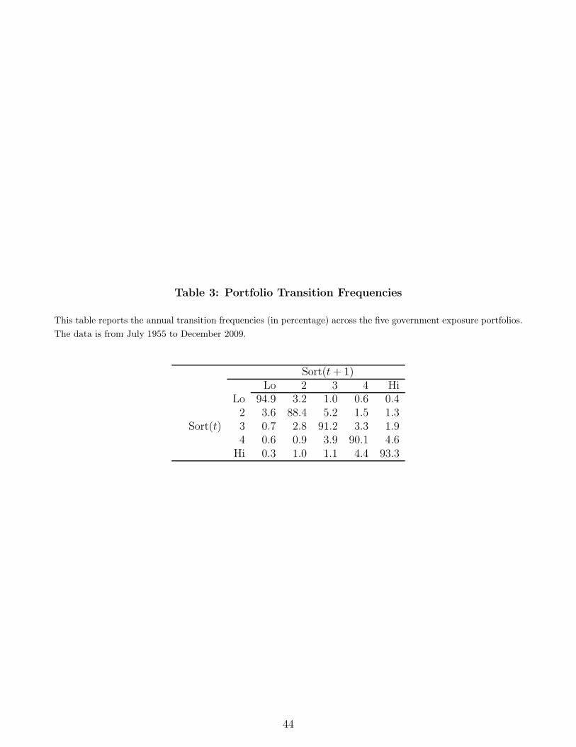
Table 3: Portfolio Transition Frequencies

This table reports the annual transition frequencies (in percentage) across the five government exposure portfolios.

The data is from July 1955 to December 2009.

Sort(t+ 1)Lo 2 3 4 Hi

Lo 94.9 3.2 1.0 0.6 0.42 3.6 88.4 5.2 1.5 1.3

Sort(t) 3 0.7 2.8 91.2 3.3 1.94 0.6 0.9 3.9 90.1 4.6

Hi 0.3 1.0 1.1 4.4 93.3

44

Table 4: Industries with High and Low Exposure to the Government Sector

This table reports a sample of industries in the high and low government exposure portfolios. Gov Expo is the

industry level measure of exposure to government spending (in percent). The data and the industry classification

is based on the 2002 Input-Output (IO) table.

GovIO Code Industry Expo Portfolio

Industries with High Exposure to the Government Sector

336414 Guided missile and space vehicle manufacturing 94.7 High336611 Ship building and repairing 67.3 High515100 Radio and television broadcasting 54.7 High541700 Scientific research and development services 47.0 High335110 Electric lamp bulb and part manufacturing 45.9 High211000 Oil and gas extraction 39.9 High511110 Newspaper publishers 28.3 High334418 Printed circuit assembly manufacturing 24.0 High334220 Broadcast and wireless communications equipment 22.6 High322120 Paper mills 20.6 High

Industries with Low Exposure to the Government Sector

311225 Fats and oils refining and blending 2.9 Low314110 Carpet and rug mills 2.9 Low311410 Frozen food manufacturing 1.8 Low311820 Cookie, cracker, and pasta manufacturing 1.7 Low339910 Jewelry and silverware manufacturing 1.2 Low312110 Soft drink and ice manufacturing 1.0 Low335224 Household laundry equipment manufacturing 0.8 Low312120 Breweries 0.8 Low3122A0 Tobacco product manufacturing 0.4 Low713950 Bowling centers 0.0 Low

45

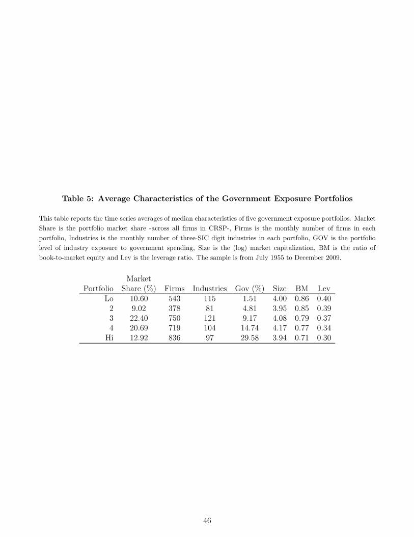
Table 5: Average Characteristics of the Government Exposure Portfolios

This table reports the time-series averages of median characteristics of five government exposure portfolios. Market

Share is the portfolio market share -across all firms in CRSP-, Firms is the monthly number of firms in each

portfolio, Industries is the monthly number of three-SIC digit industries in each portfolio, GOV is the portfolio

level of industry exposure to government spending, Size is the (log) market capitalization, BM is the ratio of

book-to-market equity and Lev is the leverage ratio. The sample is from July 1955 to December 2009.

MarketPortfolio Share (%) Firms Industries Gov (%) Size BM Lev

Lo 10.60 543 115 1.51 4.00 0.86 0.402 9.02 378 81 4.81 3.95 0.85 0.393 22.40 750 121 9.17 4.08 0.79 0.374 20.69 719 104 14.74 4.17 0.77 0.34

Hi 12.92 836 97 29.58 3.94 0.71 0.30

46

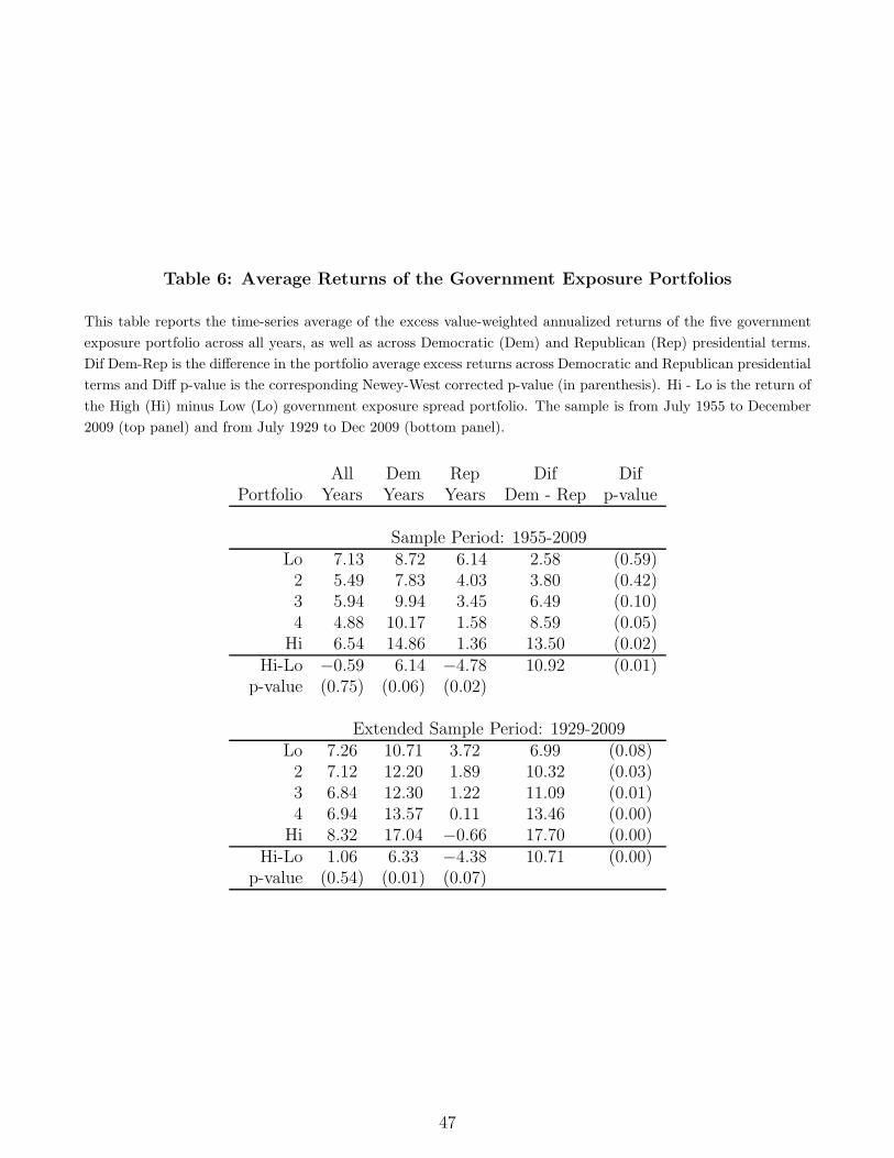
Table 6: Average Returns of the Government Exposure Portfolios

This table reports the time-series average of the excess value-weighted annualized returns of the five government

exposure portfolio across all years, as well as across Democratic (Dem) and Republican (Rep) presidential terms.

Dif Dem-Rep is the difference in the portfolio average excess returns across Democratic and Republican presidential

terms and Diff p-value is the corresponding Newey-West corrected p-value (in parenthesis). Hi - Lo is the return of

the High (Hi) minus Low (Lo) government exposure spread portfolio. The sample is from July 1955 to December

2009 (top panel) and from July 1929 to Dec 2009 (bottom panel).

All Dem Rep Dif DifPortfolio Years Years Years Dem - Rep p-value

Sample Period: 1955-2009Lo 7.13 8.72 6.14 2.58 (0.59)2 5.49 7.83 4.03 3.80 (0.42)3 5.94 9.94 3.45 6.49 (0.10)4 4.88 10.17 1.58 8.59 (0.05)

Hi 6.54 14.86 1.36 13.50 (0.02)Hi-Lo −0.59 6.14 −4.78 10.92 (0.01)

p-value (0.75) (0.06) (0.02)

Extended Sample Period: 1929-2009Lo 7.26 10.71 3.72 6.99 (0.08)2 7.12 12.20 1.89 10.32 (0.03)3 6.84 12.30 1.22 11.09 (0.01)4 6.94 13.57 0.11 13.46 (0.00)

Hi 8.32 17.04 −0.66 17.70 (0.00)Hi-Lo 1.06 6.33 −4.38 10.71 (0.00)

p-value (0.54) (0.01) (0.07)

47

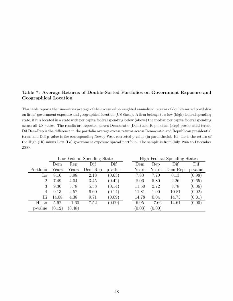
Table 7: Average Returns of Double-Sorted Portfolios on Government Exposure andGeographical Location

This table reports the time-series average of the excess value-weighted annualized returns of double-sorted portfolios

on firms’ government exposure and geographical location (US State). A firm belongs to a low (high) federal spending

state, if it is located in a state with per capita federal spending below (above) the median per capita federal spending

across all US states. The results are reported across Democratic (Dem) and Republican (Rep) presidential terms.

Dif Dem-Rep is the difference in the portfolio average excess returns across Democratic and Republican presidential

terms and Diff p-value is the corresponding Newey-West corrected p-value (in parenthesis). Hi - Lo is the return of

the High (Hi) minus Low (Lo) government exposure spread portfolio. The sample is from July 1955 to December

2009.

Low Federal Spending States High Federal Spending StatesDem Rep Dif Dif Dem Rep Dif Dif

Portfolio Years Years Dem-Rep p-value Years Years Dem-Rep p-valueLo 8.16 5.98 2.18 (0.63) 7.83 7.70 0.13 (0.98)2 7.49 4.04 3.45 (0.42) 8.06 5.80 2.26 (0.65)3 9.36 3.78 5.58 (0.14) 11.50 2.72 8.78 (0.06)4 9.13 2.52 6.60 (0.14) 11.81 1.00 10.81 (0.02)

Hi 14.08 4.38 9.71 (0.09) 14.78 0.04 14.73 (0.01)Hi-Lo 5.92 −1.60 7.52 (0.09) 6.95 −7.66 14.61 (0.00)

p-value (0.12) (0.48) (0.03) (0.00)

48

Table 8: Cross-Sectional Regressions

This table reports the results of Fama-MacBeth cross-sectional regressions of monthly excess stock returns on lagged

firm characteristics. Gov is the firm level exposure to the government sector, Size is the natural log of firm size,

B/M is the natural log of firm book-to-market ratio, Mom is firm momentum (prior cumulated 12 months returns),

Beta is the firm level current market beta computed from daily returns within the month. Dem and Rep are dummy

variables equal to one if the president is from the Democratic or Republican party, respectively. Political Contrib

is the ratio of firms’ political contribution to total assets. Fed denotes the per capita federal spending in a firm’s

headquarter state. It is measured as the cross-sectional percentile rank across all U.S. states in each year. The

table reports the average loadings for each cross-sectional regression and the corresponding Newey-West corrected

p-value (in parenthesis). The sample data is monthly from July 1955 to December 2009.

Fed× Fed×Dem× Rep× Political Dem× Rep×

Row Intercept Size B/M Mom Beta Gov Gov Contrib Gov Gov1 1.02 1.53 −0.71

(0.00) (0.01) (0.06)2 0.99 −0.07 0.13 1.00 0.34 1.00 −0.58

(0.00) (0.06) (0.00) (0.00) (0.00) (0.02) (0.05)3 1.01 −0.07 0.13 1.00 0.34 0.94 −0.63 0.38

(0.00) (0.04) (0.00) (0.00) (0.00) (0.03) (0.04) (0.00)4 1.02 1.26 −0.23 1.09 −0.91

(0.00) (0.06) (0.64) (0.10) (0.03)5 1.20 −0.09 0.18 1.08 0.29 0.90 −0.22 0.53 −0.80

(0.00) (0.01) (0.00) (0.00) (0.00) (0.10) (0.57) (0.37) (0.04)

49

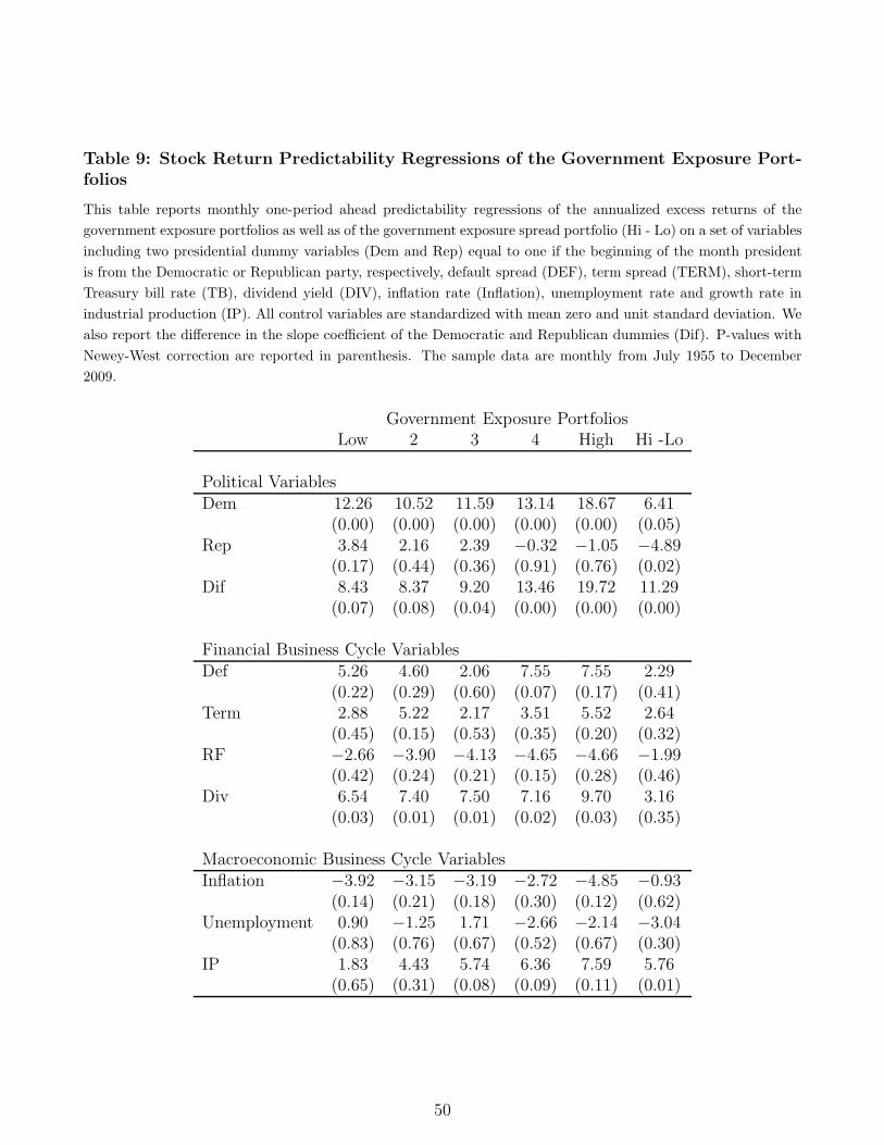
Table 9: Stock Return Predictability Regressions of the Government Exposure Port-folios

This table reports monthly one-period ahead predictability regressions of the annualized excess returns of the

government exposure portfolios as well as of the government exposure spread portfolio (Hi - Lo) on a set of variables

including two presidential dummy variables (Dem and Rep) equal to one if the beginning of the month president

is from the Democratic or Republican party, respectively, default spread (DEF), term spread (TERM), short-term

Treasury bill rate (TB), dividend yield (DIV), inflation rate (Inflation), unemployment rate and growth rate in

industrial production (IP). All control variables are standardized with mean zero and unit standard deviation. We

also report the difference in the slope coefficient of the Democratic and Republican dummies (Dif). P-values with

Newey-West correction are reported in parenthesis. The sample data are monthly from July 1955 to December

2009.

Government Exposure PortfoliosLow 2 3 4 High Hi -Lo

Political VariablesDem 12.26 10.52 11.59 13.14 18.67 6.41

(0.00) (0.00) (0.00) (0.00) (0.00) (0.05)Rep 3.84 2.16 2.39 −0.32 −1.05 −4.89

(0.17) (0.44) (0.36) (0.91) (0.76) (0.02)Dif 8.43 8.37 9.20 13.46 19.72 11.29

(0.07) (0.08) (0.04) (0.00) (0.00) (0.00)

Financial Business Cycle VariablesDef 5.26 4.60 2.06 7.55 7.55 2.29

(0.22) (0.29) (0.60) (0.07) (0.17) (0.41)Term 2.88 5.22 2.17 3.51 5.52 2.64

(0.45) (0.15) (0.53) (0.35) (0.20) (0.32)RF −2.66 −3.90 −4.13 −4.65 −4.66 −1.99

(0.42) (0.24) (0.21) (0.15) (0.28) (0.46)Div 6.54 7.40 7.50 7.16 9.70 3.16

(0.03) (0.01) (0.01) (0.02) (0.03) (0.35)

Macroeconomic Business Cycle VariablesInflation −3.92 −3.15 −3.19 −2.72 −4.85 −0.93

(0.14) (0.21) (0.18) (0.30) (0.12) (0.62)Unemployment 0.90 −1.25 1.71 −2.66 −2.14 −3.04

(0.83) (0.76) (0.67) (0.52) (0.67) (0.30)IP 1.83 4.43 5.74 6.36 7.59 5.76

(0.65) (0.31) (0.08) (0.09) (0.11) (0.01)

50

Table 10: The Presidential Investment Premium: Realized and Abnormal Returns

This table reports the average realized value-weighted returns (Ret), the Sharpe ratio, and abnormal returns (α) of the political cycle investment strategy,

across different years of the political cycle: all years, first (Year 1), second (Year 2), third (Year 3) and fourth year (Year 4) of the presidential term. The

abnormal returns of the political cycle investment strategy are obtained from three alternative asset pricing models: the CAPM (which includes only the market

factor), the Fama and French (1993) three-factor model (which includes the market, SMB and HML factors) and the Carhart (1997) four-factor model (which

includes the market, SMB, HML and Momentum factors). For each asset pricing model, we report three sets of abnormal return measures which vary in the

set of instruments used to capture time-variation in risk. α1 uses no instruments and it corresponds to the unconditional version of each asset pricing model;

α2 corresponds to the specification in which DP, DEF, TERM and RF are used as instruments; and α3 corresponds to the same specification in α2 plus a

Democratic dummy variable equal to one if the president is from the Democratic party. P-values with Newey-West correction are reported in parenthesis. The

sample data are monthly from July 1955 to December 2009.

Abnormal ReturnsSharpe CAPM Fama-French Carhart

Row Ret Ratio α1 α2 α3 α1 α2 α3 α1 α2 α3

Entire Sample Period1 All Years 5.31 0.40 5.23 6.74 4.83 5.61 6.91 4.81 3.25 5.06 3.95

(0.00) (0.01) (0.00) (0.00) (0.00) (0.00) (0.00) (0.07) (0.01) (0.00)

Within the Presidential Cycle2 Year 1 4.69 0.34 4.65 7.36 3.18 5.30 7.87 4.04 3.19 4.39 2.16

(0.20) (0.21) (0.06) (0.36) (0.16) (0.03) (0.22) (0.41) (0.21) (0.50)3 Year 2 8.28 0.72 8.30 9.59 9.06 9.39 9.96 8.32 6.98 8.01 7.25

(0.01) (0.01) (0.00) (0.00) (0.00) (0.00) (0.01) (0.03) (0.01) (0.03)4 Year 3 7.17 0.62 6.95 7.84 6.69 5.79 7.01 6.28 3.83 6.46 6.40

(0.02) (0.03) (0.01) (0.03) (0.06) (0.02) (0.03) (0.22) (0.03) (0.03)5 Year 4 1.35 0.08 1.30 2.41 0.65 1.89 2.82 0.46 −0.96 1.11 −0.21

(0.74) (0.76) (0.52) (0.52) (0.61) (0.41) (0.65) (0.79) (0.73) (0.94)

51

Table 11: Government Exposure and Cash-Flow Mean and Volatility Across Presi-dential Terms

This table examines the relationship between cash-flows (mean and volatility) and government exposure acrosspresidential terms. The table reports the time-series average slopes, with corresponding Newey-West correctedp-value in parenthesis, of several alternative specifications of the following firm level Fama-MacBeth cross-sectionalregression:

ROEit+1 = α0 + α1

Vit

Ait

+ α2DDit + α3

Dit

Bit−1

+ a4ROEit + α5Govit ×Demt + α6Govit × Rept+ εit+1

where ROE is return-on-equity defined as net income to book-equity ratio (row 1 to row 3). V/A is the ratio of

market-value of assets to book-value assets, DD is a dummy variable for nondividend-paying firms, D/B is the

ratio of dividend payments to book-equity, Gov is the level of exposure to the government sector, and Dem and

Rep are presidential dummy variables equal to one when the president is from the Democratic party or Republican

party, respectively. Row 4 reports the results from a cross-sectional regression of ε2it, where εit is the residual

from the first stage cross-sectional regression on row 3 on the presidential dummies interacted with the government

exposure variable. Dif Dem-Rep is the difference in the government exposure slope coefficient between Democratic

and Republican presidencies. The sample data is annual from 1955 to 2009.

DiffRow Intercept VA DD DB ROE Gov×Dem Gov×Rep Dem-Rep

Dependent Variable: ROEt+1

1 0.12 0.04 −0.08 0.12(0.00) (0.04) (0.00) (0.00)

2 0.06 0.02 0.00 0.95 0.09 −0.06 0.15(0.00) (0.02) (1.00) (0.00) (0.00) (0.01) (0.00)

3 0.03 0.01 0.00 0.37 0.50 0.04 −0.04 0.08(0.00) (0.03) (0.83) (0.00) (0.00) (0.01) (0.00) (0.00)

Dependent Variable: ε2it+1

4 0.05 0.07 0.05 0.02(0.04) (0.05) (0.00) (0.47)

52

Figure 1: The Government Exposure Spread Across Presidential Terms

The figure plots the average annualized value-weighted excess returns of the government exposure spread portfolio across presidential terms. The sample data

are monthly from July 1929 to December 2009.

53

Figure 2: Average Returns and Profitability of the Government Exposure Spread Across Presidential Terms

The figure plots the average annual profitability and value-weighted excess returns of the government exposure spread portfolio across presidential terms. The

measure of profitability (ROE) is adjusted to account for the control variables other than government exposure according to the regression specification in

equation (5). The sample data is from July 1955 to December 2009.

54

Government Spending, Political Cycles and the Cross ... Belo... · Government Spending, Political Cycles and the ... Government Spending, Political Cycles, ... Raghuram Rajan, Tarun

Documents