Good Practice in Large-Scale Learning for Image Classification

HAL Id: hal-00835810https://hal.inria.fr/hal-00835810

Submitted on 19 Jun 2013

HAL is a multi-disciplinary open accessarchive for the deposit and dissemination of sci-entific research documents, whether they are pub-lished or not. The documents may come fromteaching and research institutions in France orabroad, or from public or private research centers.

L’archive ouverte pluridisciplinaire HAL, estdestinée au dépôt et à la diffusion de documentsscientifiques de niveau recherche, publiés ou non,émanant des établissements d’enseignement et derecherche français ou étrangers, des laboratoirespublics ou privés.

Good Practice in Large-Scale Learning for ImageClassification

Zeynep Akata, Florent Perronnin, Zaid Harchaoui, Cordelia Schmid

To cite this version:Zeynep Akata, Florent Perronnin, Zaid Harchaoui, Cordelia Schmid. Good Practice in Large-ScaleLearning for Image Classification. IEEE Transactions on Pattern Analysis and Machine Intelligence,Institute of Electrical and Electronics Engineers, 2014, 36 (3), pp.507-520. 10.1109/TPAMI.2013.146.hal-00835810

1

Good Practice in Large-Scale Learning forImage Classification

Zeynep Akata, Student Member, IEEE, Florent Perronnin, Zaid Harchaoui, Member, IEEE,

and Cordelia Schmid, Fellow, IEEE

Abstract—We benchmark several SVM objective functions for large-scale image classification. We consider one-vs-rest, multi-class,

ranking, and weighted approximate ranking SVMs. A comparison of online and batch methods for optimizing the objectives shows that

online methods perform as well as batch methods in terms of classification accuracy, but with a significant gain in training speed. Using

stochastic gradient descent, we can scale the training to millions of images and thousands of classes. Our experimental evaluation

shows that ranking-based algorithms do not outperform the one-vs-rest strategy when a large number of training examples are

used. Furthermore, the gap in accuracy between the different algorithms shrinks as the dimension of the features increases. We

also show that learning through cross-validation the optimal rebalancing of positive and negative examples can result in a significant

improvement for the one-vs-rest strategy. Finally, early stopping can be used as an effective regularization strategy when training with

online algorithms. Following these “good practices”, we were able to improve the state-of-the-art on a large subset of 10K classes and

9M images of ImageNet from 16.7% Top-1 accuracy to 19.1%.

Index Terms—Large Scale, Fine-Grained Visual Categorization, Image Classification, Ranking, SVM, Stochastic Learning

F

1 INTRODUCTION

Image classification is the problem of assigning one or multi-

ple labels to an image based on its content. This is a standard

supervised learning problem: given a training set of labeled

images, the goal is to learn classifiers to predict labels of new

images. Large-scale image classification has recently received

significant interest from the computer vision and machine

learning communities [4], [20], [22], [48], [62], [66], [72],

[82], [89]. This goes hand-in-hand with large-scale datasets

being available. For instance, ImageNet (www.image-net.org)

consists of more than 14M images labeled with almost 22K

concepts [21], the Tiny images dataset consists of 80M im-

ages corresponding to 75K concepts [72] and Flickr contains

thousands of groups (www.flickr.com/groups) with thousands

(and sometimes hundreds of thousands) of pictures, that can

be exploited to learn object classifiers [80], [58].

Standard large-scale image classification pipelines use high-

dimensional image descriptors in combination with linear

classifiers [48], [66]. The use of linear classifiers is motivated

by their computational efficiency – a requirement when dealing

with a large number of classes and images. High-dimensional

descriptors allow separating the data with a linear classifier,

i.e., they perform the feature mapping explicitly and avoid

using nonlinear kernels. One of the simplest strategies to

learn classifiers in the multi-class setting is to train one-

vs-rest binary classifiers independently for each class. Most

image classification approaches have adopted this strategy not

• Z.Akata and F.Perronnin are with the Xerox Research Centre Europe,

Meylan, France

• Z.Akata, Z. Harchaoui and C. Schmid are with INRIA Rhone-Alpes,

Montbonnot, France.

only because of its simplicity, but also because it can be

easily parallelized on multiple cores or machines. The two

top systems at the ImageNet Large-Scale Visual Recognition

Challenge (ILSVRC) 2010 [6] used such an approach [48],

[66].

Another approach is to view image classification as a

ranking problem: given an image, the goal is to rank the labels

according to their relevance. Performance measures such as the

top-k accuracy reflect this goal and are used to report results

on standard benchmarks, such as ILSVRC. While the one-vs-

rest strategy is computationally efficient and yields competitive

results in practice, it is – at least in theory – clearly suboptimal

with respect to a strategy directly optimizing a ranking loss [9],

[17], [38], [75], [82], [86], [88].

In this paper, we examine whether these ranking approaches

scale well to large datasets and if they improve the perfor-

mance. We compare the one-vs-rest binary SVM, the multi-

class SVM of Crammer and Singer [17] that optimizes top-1

accuracy, the ranking SVM of Joachims [38] that optimizes the

rank as well as the recent weighted approximate ranking of

Weston et al. [82] that optimizes the top of the ranking list. The

datasets we consider are large-scale in the number of classes

(up to 10K), images (up to 9M) and feature dimensions (up

to 130K). For efficiency reasons we train our linear classifiers

using Stochastic Gradient Descent (SGD) algorithms [44] with

the primal formulation of the objective functions as in [11],

[67] for binary SVMs or in [54] for structured SVMs. By

using the exact same optimization framework, we truly focus

on the merits of the different objective functions, not on the

merits of the particular optimization techniques.

Our experimental evaluation confirms that SGD-based learn-

ing algorithms can work as well as batch techniques at a frac-

tion of their cost. It also shows that ranking objective functions

seldom outperform the one-vs-rest strategy. Only when a small

2

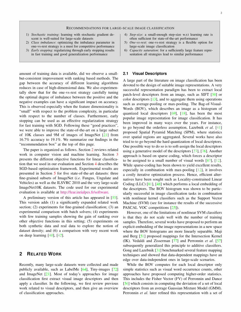
RECOMMENDATIONS FOR LARGE-SCALE IMAGE CLASSIFICATION

1) Stochastic training: learning with stochastic gradient de-scent is well-suited for large-scale datasets

2) Class imbalance: optimizing the imbalance parameter inone-vs-rest strategy is a must for competitive performance

3) Early stopping: regularizing through early stopping resultsin fast training and good generalization performance

4) Step-size: a small-enough step-size w.r.t learning rate isoften sufficient for state-of-the-art performance

5) One-vs-rest: one-vs-rest strategy is a flexible option forlarge-scale image classification

6) Capacity saturation: for a sufficiently large feature repre-sentation all strategies lead to similar performance

amount of training data is available, did we observe a small-

but-consistent improvement with ranking based methods. The

gap between the accuracy of different learning algorithms

reduces in case of high-dimensional data. We also experimen-

tally show that for the one-vs-rest strategy carefully tuning

the optimal degree of imbalance between the positive and the

negative examples can have a significant impact on accuracy.

This is observed especially when the feature dimensionality is

“small” with respect to the problem complexity, in particular

with respect to the number of classes. Furthermore, early

stopping can be used as an effective regularization strategy

for fast training with SGD. Following these “good practices”,

we were able to improve the state-of-the-art on a large subset

of 10K classes and 9M of images of ImageNet [21] from

16.7% accuracy to 19.1%. We summarize our findings in the

“recommendation box” at the top of this page.

The paper is organized as follows. Section 2 reviews related

work in computer vision and machine learning. Section 3

presents the different objective functions for linear classifica-

tion that we used in our evaluation and Section 4 describes the

SGD-based optimization framework. Experimental results are

presented in Section 5 for five state-of-the-art datasets: three

fine-grained subsets of ImageNet (i.e. Fungus, Ungulate and

Vehicles) as well as the ILSVRC 2010 and the very large-scale

ImageNet10K datasets. The code used for our experimental

evaluation is available at http://lear.inrialpes.fr/software.

A preliminary version of this article has appeared in [55].

This version adds (1) a significantly expanded related work

section; (2) experiments for fine-grained classification; (3) an

experimental comparison with batch solvers; (4) experiments

with few training samples showing the gain of ranking over

other objective functions in this setting; (5) experiments on

both synthetic data and real data to explore the notion of

dataset density; and (6) a comparison with very recent work

on deep learning [40], [42].

2 RELATED WORK

Recently, many large-scale datasets were collected and made

publicly available, such as LabelMe [64], Tiny-images [72]

and ImageNet [21]. Most of today’s approaches for image

classification first extract visual image descriptors and then

apply a classifier. In the following, we first review previous

work related to visual descriptors, and then give an overview

of classification approaches.

2.1 Visual Descriptors

A large part of the literature on image classification has been

devoted to the design of suitable image representations. A very

successful representation paradigm has been to extract local

patch-level descriptors from an image, such as SIFT [50] or

color descriptors [13], and to aggregate them using operations

such as average-pooling or max-pooling. The Bag-of-Visual-

Words (BOV), which describes an image as a histogram of

quantized local descriptors [69], [18], has been the most

popular image representation for image classification. It has

been improved in many ways over the years. For instance,

to go beyond the orderless assumption, Lazebnik et al. [41]

proposed Spatial Pyramid Matching (SPM), where statistics

over spatial regions are aggregated. Several works have also

tried to to go beyond the hard quantization of local descriptors.

One possible way to do so is to soft-assign the local descriptors

using a generative model of the descriptors [27], [76]. Another

approach is based on sparse coding, which forces a descriptor

to be assigned to a small number of visual words [87], [12].

While sparse-coding has been shown to yield excellent results,

especially in combination with max-pooling [12], it involves

a costly iterative optimization process. Hence, efficient alter-

natives have been sought such as Locality-constrained Linear

Coding (LLC) [81], [48] which performs a local embedding of

the descriptors. The BOV histogram was shown to be partic-

ularly successful in image classification tasks in combination

with nonlinear kernel classifiers such as the Support Vector

Machine (SVM) (see for instance the results of the successive

PASCAL VOC competitions [25]).

However, one of the limitations of nonlinear SVM classifiers

is that they do not scale well with the number of training

samples. Therefore, several works have proposed to perform an

explicit embedding of the image representations in a new space

where the BOV histograms are more linearly separable. Maji

and Berg [51] proposed mappings for the Intersection Kernel

(IK). Vedaldi and Zisserman [77] and Perronnin et al. [57]

subsequently generalized this principle to additive classifiers.

Gong and Lazebnik [31] benchmarked several feature mapping

techniques and showed that data-dependent mappings have an

edge over data-independent ones in large-scale scenarios.

While the BOV computes for each local descriptor only

simple statistics such as visual word occurrence counts, other

approaches have proposed computing higher-order statistics.

This includes the Fisher Vector (FV) of Perronnin and Dance

[56] which consists in computing the deviation of a set of local

descriptors from an average Gaussian Mixture Model (GMM).

Perronnin et al. later refined this representation with a set of

3

normalization steps [57]. Other higher-order representations

have been proposed including the Vector of Locally Aggre-

gated Descriptors (VLAD) [36] and the Super Vector (SV)

[90]. Since these techniques perform an explicit embedding

of local descriptors in a very high-dimensional space, they

typically work well with simple linear classifiers. Chatfield et

al. [16] benchmarked five local descriptor encoding techniques

(BOV with hard coding, soft coding and sparse coding as well

as SV and FV coding); the FV of [57] was shown to yield the

best results on two standard datasets. A weakness of high-

dimensional representations such as the FV is that they take

a lot of space in RAM or on disk [66], [49]. Consequently,

they are difficult to scale to large datasets and several works

proposed more compact features for classification. One line

of work consists in describing an image with a set of high-

level concepts based on object classifiers [80], [73], [7] or

object detectors [47]. Coding techniques such as Product

Quantization (PQ) [35] have also been used to compress the

data [66], [60], [78]. While Sanchez and Perronnin proposed to

learn classifiers using Stochastic Gradient Descent (SGD) (see

section 2.3) and on-the-fly decompression of training samples

[66], Vedaldi and Zisserman showed that classifiers can be

learned in the compressed space directly [78].

The standard feature extraction pipeline that aggregates

patch descriptors can be criticized as being too shallow to learn

complex invariances and high-level concepts. Recently, several

large-scale works have considered the learning of features

directly from pixel values using deeper architectures [5], [42],

[40]. One of the crucial factors to obtain good results when

learning deep architectures with millions if not billions of

parameters seems to be the availability of vast amounts of

training data (see section 10.1 in [5]). In [42], [19], the features

are learned using a deep autoencoder which is constructed

by replicating three times the same three layers – made of

local filtering, local pooling and contrast normalization – thus

resulting in an architecture with 9 layers. The learned features

were shown to give excellent results in combination with a

simple linear classifier. In [40], a deep network with 8 layers

was proposed where the first 5 layers are convolutional [43],

[45], [34], the remaining three are fully connected and the

output of the last fully connected layer is fed to a softmax

which produces a distribution over the class labels.

In this work, we will use mostly the FV representation as

it was shown to yield excellent results in large-scale classi-

fication while requiring only modest computational resources

[66]. However, we believe our conclusions to be generic and

applicable to other image features.

2.2 Classifier Strategies

We underline that in most previous works tackling large-scale

visual data sets, the objective function that is optimized is

always the same: one binary SVM is learned per class in a

one-vs-rest fashion [20], [66], [48], [62]. Some approaches use

simple classifiers such as nearest-neighbor (NN) [72]. While

exact NN can provide a competitive accuracy when compared

to SVMs as in [82], [20], it is not straightforward to scale

to large data sets. On the other hand, Approximate Nearest

Neighbor (ANN) can perform poorly on high-dimensional

image descriptors (significantly worse than one-vs-rest SVMs)

while still being much more computationally intensive [82].

One-vs-rest (OVR) strategies offer several advantages such as

the speed and simplicity as compared to multiclass classifiers

(see [61] from Rifkin and Klautau as a defense of OVR).

Indeed, OVR classifiers can be trained efficiently by decom-

posing the problem into independent per class problems.

On the other hand, several versions of multi-class SVMs

were proposed. In [85], Weston and Watkins propose a multi-

class SVM with a loss function that consists in summing

the losses incurred by each class-wise score. Note that this

version of multi-class SVM is statistically not consistent for

large samples [71]. Lee et al. [46] introduced a statistically

consistent version of multi-class SVM, which can be thought

of a “hinge-loss” counterpart of multinomial classification. In

this work, we use the multiclass SVM formulation of Crammer

and Singer from [17], a computationally attractive variant that

was proven to be consistent for large-scale problems.

Many alternative approaches for multi-class classification

were proposed in the literature. In [24], Dietterich and Bakiri

introduce error correcting codes as a basis of multiclass

classification. In [1] Allwein et al. combine several multiclass

classifiers using AdaBoost. In [79], Vural and Dy approach the

problem from the decision trees perspective by partitioning the

space in N − 1 regions.

When the target loss function is not classification accuracy

but a more sophisticated performance measure such as mean-

average-precision, a natural approach is to build ranking algo-

rithms. In [38], Joachims proposed a ranking SVM, allowed to

rank highly related documents on the higher ranks of the list.

In [32], Grangier et al. improve the baseline ranking SVM by

giving weights to classifiers. Usunier et al. [75] penalize the

loss encountered at the top of the list more than the bottom.

Another ranking framework [83] from Weston et al. uses linear

classifiers trained with SGD and a novel sampling trick to

approximate ranks. To break the time-complexity of training to

sub-linear in the number of classes, various approaches have

been proposed which employ tree structures [52], [4], [29],

[14], [53], [30]. In [8], Beygelzimer et al. create a model for

error-limiting reduction in learning. According to this model,

the tree (multiclass) reduction has a slightly larger loss rate

than binary classifiers. The reader may refer to [63] for an

extended survey of top-down approaches for classification.

2.3 Algorithms and Solvers

Here, we review the currently publicly available solvers for

SVM-like classification and ranking algorithms. We shall

not review other approaches, as we do not include them in

our benchmarks. There are two main families of algorithms

for optimization SVM objectives: batch algorithms, and on-

line/incremental algorithms.

State-of-the-art batch optimization algorithms for non-linear

SVMs are based on a variant of coordinate-descent called se-

quential minimal optimization (SMO)[59]. The main strength

of batch approaches is the high robustness to the settings of

the algorithms parameters, that is initialization, line-search,

4

number of iterations, etc. Such algorithms are implemented

in the most popular toolboxes LibSVM [15] from Chang et

al., SVMlight [37], and Shogun [28]. State-of-the art batch

algorithms for linear SVMs are based on coordinate-descent

approaches with second-order acceleration. The widely used

LibLinear toolbox [33] from Hsieh et al. provides an efficient

implementation of such algorithms. The weakness of batch

methods is the difficulty to scale up to large datasets.

State-of-the-art stochastic (online) optimization algorithms

for linear SVMs are based on stochastic gradient descent

(SGD). The well known online SVM solver Pegasos [67] from

Shalew-Shwartz et al. and libSGD [10] from Bottou provide

an implementation of these algorithms. The main strength of

SGD algorithms is their built-in ability to scale up to large

datasets. However, without a careful setting of the parameters,

SGD algorithms can have slow convergence and struggle to

match the performance of their batch algorithm counterparts.

In this paper, we highlight the “golden rules” while using SGD

to get competitive performance with batch solvers, and provide

empirical evidence of the success of our methodology.

3 OBJECTIVE FUNCTIONS

Let S = (xi, yi), i = 1 . . . N be the training set where

xi ∈ X is an image descriptor, yi ∈ Y is the associated label

and Y is the set of possible labels. Let C = |Y| denote the

number of classes. We shall always take X = RD.

Supervised learning corresponds to minimizing the empiri-

cal risk with a regularization penalty

MinimizeW

λ2 Ω(W) + L(S;W) , (1)

where W is the weight matrix stacking the weight vectors

corresponding to each subproblem. The objective decomposes

into the empirical risk

L(S;W) :=1

N

N∑

i=1

L(xi, yi;W) (2)

with L(xi, yi;W) a surrogate loss of the labeled example

(xi, yi), and the regularization penalty

Ω(W) :=

C∑

c=1

‖wc‖2 (3)

The parameter λ ≥ 0 controls the trade-off between the

empirical risk and the regularization. We first briefly review

the classical binary SVM. We then proceed with the multiclass,

ranking and weighted approximate ranking SVMs. We finally

discuss the issue of data re-weighting.

3.1 Binary One-Vs-Rest SVM (OVR)

In the case of the one-vs-rest SVM, we assume that we have

only two classes and Y = −1,+1. Let 1(u) = 1 if u is

true and 0 otherwise. The 0-1 loss 1(yiwTxi < 0) is upper-

bounded by

LOVR(xi, yi;w) = max0, 1 − yiwTxi (4)

If we have more than two classes, then one transforms the

C-class problem into C binary problems and trains indepen-

dently C one-vs-rest classifiers.

3.2 Beyond Binary Classification

In the following sections, we treat the classes jointly and the

label set contains more than two labels i.e. Y = 1, . . . , C.

Let wc, c = 1 . . . C denote the C classifiers corresponding

to each of the C classes. In this case, W is a C × Ddimensional vector obtained by concatenating the different

wc’s. We denote by ∆(y, y) the loss incurred for assigning

label y while the correct label was y. In this work, we focus

on the 0/1 loss, i.e. ∆(y, y) = 0 if y = y and 1 otherwise. In

what follows, we assume that we have one label per image to

simplify the representation.

Multiclass SVM (MUL). There exist several flavors of the

multiclass SVM such as the Weston and Watkins [84] and

the Crammer and Singer [17] formulations (see [71] for

a comprehensive review). Both variants propose a convex

surrogate loss to ∆(yi, yi) with

yi = arg maxy

wTy xi, (5)

i.e. the loss incurred by taking the highest score as the pre-

dicted label. We choose the Crammer and Singer formulation,

corresponding to

LMUL(xi, yi;w) = maxy

∆(yi, y) + wTy xi

− wTyixi (6)

which provides a tight bound on the misclassification er-

ror [74]. Note that this can be viewed as a particular case

of the structured SVM [74].

Ranking SVM (RNK). Joachims [38] considers the problem

of ordering pairs of documents. Adapting the ranking frame-

work to our problem the goal is, given a sample (xi, yi) and

a label y 6= yi, to enforce wyixi > w

Ty xi. The rank of label

y for sample x can be written as:

r(x, y) =

C∑

c=1

1(wTc x ≥ w

Ty x) (7)

Given the triplet (xi, yi, y), 1(wTc x ≥ w

Ty x) is upper-

bounded by:

Ltri(xi, yi, y;w) = max0,∆(yi, y) − wTyi

xi + wTy xi (8)

Therefore, the overall loss of (xi, yi) writes as:

LRNK(xi, yi;w) =

C∑

y=1

max0,∆(yi, y) − (wyi− wy)T

xi

(9)

Weighted Approximate Ranking SVM (WAR). An issue

with the Ranking SVM (RNK) is that the loss is the same

when going from rank 99 to 100 or from rank 1 to rank 2.

However, in most practical applications, one is interested in the

top of the ranked list. As an example, in ILSVRC the measure

used during the competition is a loss at rank 5. Usunier et al.

[75] therefore proposed to minimize a function of the rank

which gives more weight to the top of the list.

Let α1 ≥ α2 ≥ . . . αC ≥ 0 be a set of C coefficients. For

sample (xi, yi) the loss is ℓr(xi,yi) with ℓ defined as

ℓk =

k∑

j=1

αj (10)

5

The penalty incurred by going from rank k to k + 1 is αk.

Hence, a decreasing sequence αjj≥1 implies that a mistake

on the rank when the true rank is at the top of the list incurs

a higher loss than a mistake on the rank when the true rank is

lower in the list. We note that this Ordered Weighted Ranking

(OWR) objective function is generic and admits as special

cases the multiclass SVM of Crammer and Singer (α1 = 1and αj = 0 for j ≥ 2) and the ordered pairwise ranking SVM

of Joachims (αj = 1 , ∀i).

While [75] proposes an upper-bound on the loss, Weston et

al. [82] propose an approximation. We follow [82] which is

more amenable to large-scale optimization and write:

LWAR(xi, yi;w) =

C∑

y=1

ℓr∆(xi,yi)Ltri(xi, yi, y;w)

r∆(xi, yi), (11)

where

r∆(x, y) =C

∑

c=1

1(wTc x+ ∆(y, c) ≥ w

Ty x) (12)

is a regularized rank. Following [82], we choose αj = 1/j.As opposed to other works [86], [88], this does not optimize

directly standard information retrieval measures such as Av-

erage Precision (AP). However, it mimics their behavior by

putting emphasis on the top of the list, works well in practice

and is highly scalable.

Data Rebalancing. When the training set is unbalanced,

i.e. when some classes are significantly more populated than

others, it can be beneficial to reweight the data. This imbalance

can be extreme in the one-vs-rest case when one has to deal

with a large number of classes C as the imbalance between the

positive class and the negative class is on average C−1. In the

binary case, the reweighting can be performed by introducing

a parameter ρ and the empirical risk then writes as:

ρ

N+

∑

i∈I+

LOVR(xi, yi;w) +1 − ρ

N−

∑

i∈I−

LOVR(xi, yi;w) (13)

where I+ (resp. I−) is the set of indices of the positive (resp.

negative) samples and N+ (resp. N−) is the cardinality of this

set. Note that ρ = 1/2 corresponds to the natural rebalancing

of the data, i.e. in such a case one gives as much weight to

positives and negatives.

When training all classes simultaneously, introducing one

parameter per class is computationally intractable. It would

require cross-validating C parameters jointly, including the

regularization parameter. In such a case, the natural re-

balancing appears to be the most natural choice. In the multi-

class case, the empirical loss becomes:

1

C

C∑

c=1

1

Nc

∑

i∈Ic

LMUL(xi, yi;w) (14)

where Ic = i : yi = c and Nc is the cardinality of this set.

One can perform a similar rebalancing in the case of LRNK

and LWAR.

4 OPTIMIZATION ALGORITHMS

We employ Stochastic Gradient Descent (SGD) to learn linear

classifiers in the primal [67], [11]. Such an approach has

recently gained popularity in the computer vision community

for large-scale learning [57], [58], [82], [66], [48], [62]. In the

following, we describe the optimization algorithms for various

objective functions and give implementation details.

4.1 Stochastic Training

Training with Stochastic Gradient Descent (SGD) consists at

each step in choosing a sample at random and updating the

parameters w using a sample-wise estimate of the regularized

risk. In the case of ROVR and RMUL, the sample is simply a pair

(xi, yi) while in the case of RRNK and RWAR it consists of a

triplet (xi, yi, y) where y 6= yi. Let zt denote the sample drawn

at step t (whether it is a pair or a triplet) and let R(zt;w) be

the sample-wise estimate of the regularized risk. w is updated

as follows:

w(t) = w

(t−1) − ηt∇w=w(t−1)R(zt;w) (15)

where ηt is the step size.

We provide in Table 1 the sampling and update procedures

for the objective functions used in our evaluation, assuming

no rebalancing of the data. For ROVR, RMUL and RRNK,

these equations are straightforward and optimize exactly the

regularized risk. For RWAR it is only approximate as it does

not compute exactly the value of r∆(xi, yi), but estimates it

from the number of samples k which were drawn before a

violating sample y such that Ltri(xi, yi, y;w) > 0 was found.

If k samples were drawn, then:

r∆(xi, yi) ≈ ⌊C − 1

k⌋. (16)

For a large number of classes, this approximate procedure

is significantly faster than the exact one (see [82] for more

details). Note also that we implement the regularization by

penalizing the squared norm of w, while [82] actually bounds

the norm of w. We tried both strategies and observed that they

provide similar results in practice.

4.2 Implementation Details

We use as basis for our code the SGD library for binary

classification available on Bottou’s website (version 1.3)[10].

This is an optimized code that includes fast linear algebra and

a number of optimizations such as the use of a scale variable

to update w only when a loss is incurred.

We now discuss a number of implementation details.

Bias. Until now, we have not considered the bias in our ob-

jective functions. This corresponds to an additional parameter

per class. Following common practice, we add one constant

feature to each observation xi. As is the case in Bottou’s code,

we do not regularize this additional dimension.

Stopping Criterion. Since at each step in SGD we have a

noisy estimate of the objective function, this value cannot be

used for stopping. Therefore, in all our experiments, we use

a validation set and stop iterating when the accuracy does not

increase by more than a threshold θ.

6

Sampling Update

ROVR Draw (xi, yi) from S. δi = 1 if LOVR(xi, yi;w) > 0, 0 otherwise.

w(t) = (1 − ηtλ)w(t−1) + ηtδixiyi

RMUL Draw (xi, yi) from S. y = arg maxy ∆(yi, y) + w′yxi and δi =

1 if y 6= yi

0 otherwise.

w(t)y =

8

>

<

>

:

w(t−1)y (1 − ηtλ) + δiηtxi if y = yi

w(t−1)y (1 − ηtλ) − δiηtxi if y = y

w(t−1)y (1 − ηtλ) otherwise.

RRNK Draw (xi, yi) from S. δi = 1 if Ltri(xi, yi, y;w) > 0, 0 otherwise.

Draw y 6= yi from Y . w(t)y =

8

>

<

>

:

w(t−1)y (1 − ηtλ) + δiηtxi if y = yi

w(t−1)y (1 − ηtλ) − δiηtxi if y = y

w(t−1)y (1 − ηtλ) otherwise.

RWAR Draw (xi, yi) from S. δi = 1 if y s.t. Ltri(xi, yi, y;w) > 0 was sampled, 0 otherwise.For k = 1, 2, . . . , C − 1, do:

Draw y 6= yi from Y.If Ltri(xi, yi, y;w) > 0, break.

w(t)y =

8

>

<

>

:

w(t−1)y (1 − ηtλ) + δiℓ⌊ C−1

k⌋ηtxi if y = yi

w(t−1)y (1 − ηtλ) − δiℓ⌊ C−1

k⌋ηtxi if y = y

w(t−1)y (1 − ηtλ) otherwise.

TABLE 1

Sampling and update equations for various objective functions.

Regularization. While a vast majority of works on large-

margin classification regularize explicitly by penalizing the

squared norm of w or by bounding it, regularizing implicitly

by early stopping is another option [2]. In such a case, one sets

λ = 0 and iterates until the performance converges (or starts

descreasing) on a validation set. In our experiments, applying

this strategy yields competitive results.

Step Size. To guarantee converge to the optimum, the sequence

of step sizes should satisfy∑∞

t=1 ηt = ∞ and∑∞

t=1 η2t <∞.

Assuming λ > 0, the usual choice is ηt = 1/λ(t+ t0), where

t0 is a parameter. Bottou provides in his code a heuristic to set

t0. We tried to cross-validate t0 but never observed significant

improvements. However, we also experimented with a fixed

step size η as in [2], [82].

Rebalancing. All sampling/update equations in Table 1 are

based on non-rebalanced objective functions. To rebalance

the data, we can modify either the sampling or the update

equations. We chose the first alternative since, in general,

it led to faster convergence. If we take the example of

LOV R then the sampling is modified as follows: draw y =+1 with probability ρ, y = −1 with probability 1 − ρ. Then

draw xi such that yi = y.

5 EXPERIMENTS

In Section 5.1 we describe our experimental setup. In Sec-

tion 5.2, we provide a detailed analysis of the different objec-

tive functions and parameters for three fine-grained subsets of

ImageNet (Fungus, Ungulate, Vehicle). We believe that these

fine-grained datasets can provide useful insights about the

different objective functions since they correspond to different

class densities as shown in [20]. In Section 5.4, we provide

results on ImageNet10K.

5.1 Experimental Setup

In this section, we describe the datasets and image descriptors

used in our experiments.

Total # of Partition

images classes train val test

Fungus 88K 134 44K 5K 39KUngulate 183K 183 91.5K 5K 86.5K

Vehicle262 226K 262 113K 5K 108K

ILSVRC10 1.4M 1,000 1.2M 50K 150KImageNet10K 9M 10,184 4.5M 50K 4.45M

TABLE 2

The datasets used in our evaluation.

Datasets. For our fine-grained image categorization experi-

ments, we use three subsets of ImageNet: Fungus, Ungulate

and Vehicle [20]. These datasets contain only the leaf nodes

under the respective parent class (i.e. fungus, ungulate or

vehicle) in the hierarchy of ImageNet. Unless stated otherwise,

we used the following set-up: half of the data is used for

training, 5K images for validation and the remainder for

testing.

For our large-scale experiments, we use ILSVRC 2010 [6]

and ImageNet10K [20]. For ILSVRC2010, we follow the stan-

dard training/validation/testing protocol. For ImageNet10K,

we follow [66] and use half of the data for training, 50K

images for validation and the remainder for testing. The

properties of the datasets are summarized in Table 2.

In all experiments, we compute the (flat) top-1 or top-5

accuracy per class and report the average as in [20], [66],

[82]. We could also have used a hierarchical loss which takes

into account the fact that some errors are more costly than

others. The choice of a flat vs. a hierarchical loss is directly

related to the choice of the cost function ∆ (see section 3).

In preliminary experiments, this choice had only very limited

impact on the ranking of the different objective functions.

This effect was also observed during the ILSVRC 2010 and

2011 competitions which might explain why the hierarchical

measure was dropped in 2012. In what follows we report only

accuracies with a flat loss.

Image Descriptors. Before feature extraction, we resize the

7

images to 100K pixels (if larger) while keeping the aspect

ratio. We extract approx. 10K SIFT descriptors [50] at 5

scales for 24×24 patches every 4 pixels. The SIFT descriptors

are reduced from 128-dim to 64-dim using PCA. They are

then aggregated into an image-level signature (e.g. BOV or

FV) using a probabilistic visual vocabulary, i.e. a Gaussian

Mixture Model (GMM). By default, we use Fisher Vectors

(FV) with N =256 Gaussians. We also report results with the

bag of visual words (BOV) given its popularity in large-scale

classification [20], [82]. Our default BOV uses N = 1, 024codewords. Note that our purpose is not to compare the BOV

and FV representations in this work (see [16] for such a

comparison). Unless it is stated otherwise, we use spatial

pyramids with R = 4 regions (the entire image and three

horizontal stripes).

Our experiments on large-scale datasets require image sig-

natures to be compressed. For the FV we employ Product

Quantization (PQ) [35]. We use sub-vectors of 8 dimensions

and 8 bits per sub-vector. This setting was shown to yield

minimal loss of accuracy in [66]. For the BOV we use

Scalar Quantization with 8 bits per dimension as suggested

in [20]. Signatures are decompressed on-the-fly by the SGD

routines [66].

5.2 Analysis on Fine Grained Datasets

Distinguishing between semantically related categories which

are also visually very similar is referred to as fine-grained

visual categorization (see [23] for a study of the relationship

between semantic and visual similarity in ImageNet). It has

several applications such as the classification of mushrooms

for edibility, animals for environmental monitoring or vehicles

for traffic related applications. In this section we analyze the

performance of the objective functions described in Section 3

in the context of fine-grained visual categorization. We report

results on three subsets of ImageNet: Fungus, Ungulate and

Vehicle [20].

Comparison between SGD and Batch Methods.

It is known that SGD can perform as well as batch solvers

for OVR SVMs at a fraction of the cost [11], [67]. However,

public SGD solvers do not exist for other SVM formulations

such as w-OVR, MUL, RNK or WAR. Hence, as a sanity

check, we compared our w-OVR and MUL SGD solvers to

publicly available batch solvers. We compared our w-OVR

SGD to LibSVM [15] and MUL SGD to LibLINEAR [26] and

SVMlight [39]. Given the cost of training batch solvers, we

restrict our experiments to the small dimensional BOV vectors

(N = 1, 024 × R = 4 → 4, 096 dimensions). Furthermore,

we perform training on subsets of the full training sets: for

each class we use 10, 25, 50 and 100 random samples within

the training set. We repeat the experiments 5 different times

for 5 random subsets of training images. Top-1 classification

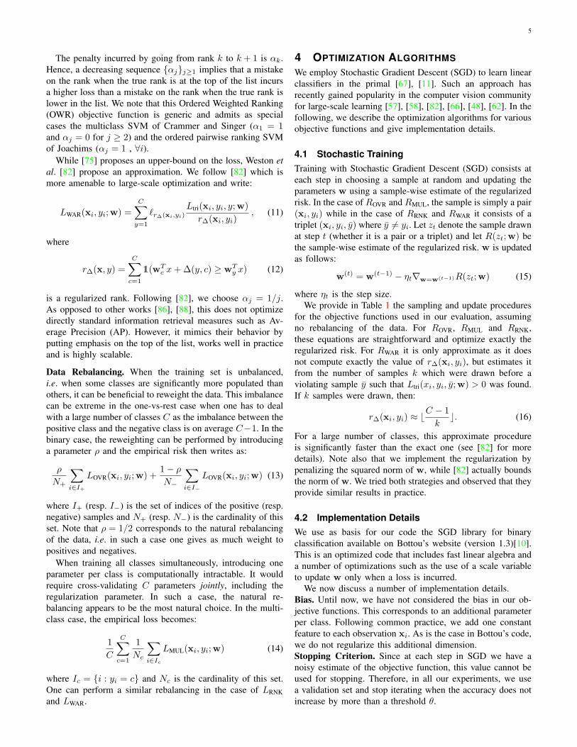
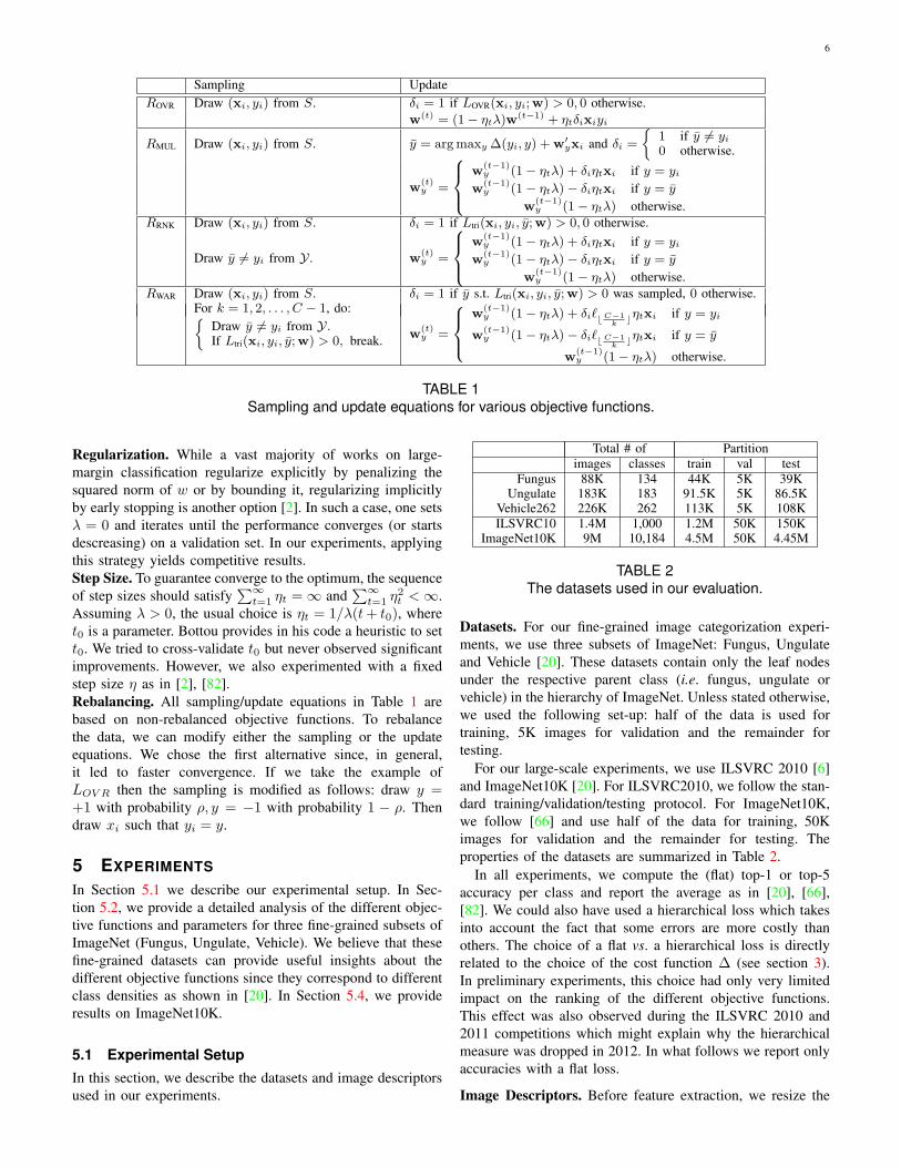
accuracy is reported in Figure 1 and 2.

These experiments show that stochastic and batch solvers

perform on par for w-OVR and MUL SVMs. Somewhat

surprisingly, SGD solvers even seem to have a slight edge

over batch solvers, especially for the MUL SVM. This might

be because SGD uses as stopping criterion the accuracy on the

(a) w-OVR SVM: LibSVM vs. SGD

LibSVM (batch) / SGD (online)

Fungus Ungulate Vehicle

10 12 / 7 31 / 18 107 / 3925 95 / 16 175 / 36 835 / 11950 441 / 38 909 / 67 3,223 / 271

100 1,346 / 71 3,677 / 133 11,679 / 314

(b) MUL SVM: SVMlight vs. SGD

SVMlight (batch) / SGD (online)

Fungus Ungulate Vehicle

10 45 / 36 324 / 81 557 / 20925 99 / 72 441 / 198 723 / 36950 198 / 261 855 / 420 1,265 / 747

100 972 / 522 1,674 / 765 3,752 / 1,503

TABLE 3

Average training time (in CPU seconds) on Fungus,

Ungulate, Vehicle for 10, 25, 50, 100 training samples

per class using 4,096-dim BOV.

validation set measured with the true target loss (top-1 loss in

this case). In contrast, batch solvers stop upon convergence

of a surrogate objective function on the training set. The

training times of SGD and batch solvers are reported in Table

3 (in CPU seconds on 32GBs RAM double quad-core multi-

threaded servers using a single CPU). As expected, the CPU

time of SGD solvers is significantly smaller than for batch

solvers and the difference increases for larger training sets.

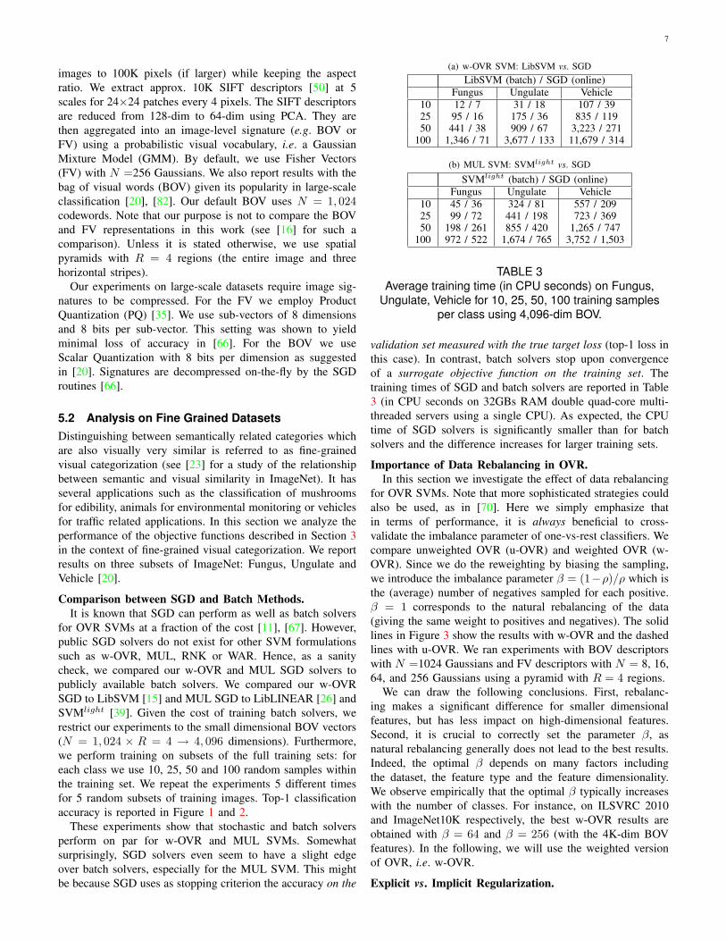
Importance of Data Rebalancing in OVR.

In this section we investigate the effect of data rebalancing

for OVR SVMs. Note that more sophisticated strategies could

also be used, as in [70]. Here we simply emphasize that

in terms of performance, it is always beneficial to cross-

validate the imbalance parameter of one-vs-rest classifiers. We

compare unweighted OVR (u-OVR) and weighted OVR (w-

OVR). Since we do the reweighting by biasing the sampling,

we introduce the imbalance parameter β = (1−ρ)/ρ which is

the (average) number of negatives sampled for each positive.

β = 1 corresponds to the natural rebalancing of the data

(giving the same weight to positives and negatives). The solid

lines in Figure 3 show the results with w-OVR and the dashed

lines with u-OVR. We ran experiments with BOV descriptors

with N =1024 Gaussians and FV descriptors with N = 8, 16,

64, and 256 Gaussians using a pyramid with R = 4 regions.

We can draw the following conclusions. First, rebalanc-

ing makes a significant difference for smaller dimensional

features, but has less impact on high-dimensional features.

Second, it is crucial to correctly set the parameter β, as

natural rebalancing generally does not lead to the best results.

Indeed, the optimal β depends on many factors including

the dataset, the feature type and the feature dimensionality.

We observe empirically that the optimal β typically increases

with the number of classes. For instance, on ILSVRC 2010

and ImageNet10K respectively, the best w-OVR results are

obtained with β = 64 and β = 256 (with the 4K-dim BOV

features). In the following, we will use the weighted version

of OVR, i.e. w-OVR.

Explicit vs. Implicit Regularization.

8

10 25 50 1004

6

8

10

12

14

Number of Images N

Top−

1 Ac

cura

cy (i

n %

)

w−OVR (SGD)w−OVR (libSVM)

(a) Fungus

10 25 50 1005

10

15

Number of Images N

Top−

1 Ac

cura

cy (i

n %

)

w−OVR (SGD)w−OVR (libSVM)

(b) Ungulate

10 25 50 100

8

10

12

14

16

18

20

22

24

Number of Images N

Top−

1 Ac

cura

cy (i

n %

)

w−OVR (SGD)w−OVR (libSVM)

(c) Vehicle

Fig. 1. Comparison of SGD and libSVM for optimizing the w-OVR SVM using 4,096-dim BOV descriptors. From left to

right: Fungus, Ungulate and Vehicle.

10 25 50 1004

5

6

7

8

9

10

11

12

13

Number of Images N

Top−

1 Ac

cura

cy (i

n %

)

Multiclass (SGD)Multiclass (SVMlight)Multiclass (LibLinear)

(a) Fungus

10 25 50 1004

5

6

7

8

9

10

11

12

13

Number of Images N

Top−

1 Ac

cura

cy (i

n %

)

Multiclass (SGD)Multiclass (SVMlight)Multiclass (LibLinear)

(b) Ungulate

10 25 50 1008

10

12

14

16

18

20

22

24

Number of Images N

Top−

1 Ac

cura

cy (i

n %

)

Multiclass (SGD)Multiclass (SVMlight)Multiclass (LibLinear)

(c) Vehicle

Fig. 2. Comparison of SGD, SVMlight and LibLinear for optimizing the MUL SVM using using 4,096-dim BOV. From

left to right: Fungus, Ungulate and Vehicle.

1 2 4 8 16 32 6410

12

14

16

18

20

22

Weight β

Top−

1 A

ccur

acy

(in %

)

BOV (N=1,024) + SPFV (N=8) + SPFV (N=16) + SPFV (N=32) + SPFV (N=64) + SPFV (N=128) + SPFV (N=256) + SP

(a) Fungus

1 2 4 8 16 32 64

14

16

18

20

22

24

26

28

30

32

Weight β

Top−

1 A

ccur

acy

(in %

)

BOV (N=1,024) + SPFV (N=8) + SPFV (N=16) + SPFV (N=32) + SPFV (N=64) + SPFV (N=128) + SPFV (N=256) + SP

(b) Ungulate

1 2 4 8 16 32 6420

22

24

26

28

30

32

34

36

38

40

42

Weight β

Top−

1 A

ccur

acy

(in %

)

BOV (N=1,024) + SPFV (N=8) + SPFV (N=16) + SPFV (N=32) + SPFV (N=64) + SPFV (N=128) + SPFV (N=256) + SP

(c) Vehicle

Fig. 3. Influence of data rebalancing in weighted One-vs-Rest (w-OVR). The value of the weight parameter indicates

the number of negative training samples for one positive sample (solid lines). The results of unweighted One-vs-Rest

(u-OVR) are shown with dashed lines.

We run experiments on high-dimensional features (the

130K-dim FV for N =256 and R =4), i.e. for which

regularization is supposed to have a significant impact. The

following experiments focus on w-OVR but we obtained very

similar results for MUL, RNK and WAR. We compare three

regularization strategies:

(i) Using explicit regularization (λ > 0) and a de-

creasing step size ηt = 1/(λ(t + t0) [10]. Setting

t0 correctly is of paramount importance for fast

convergence and Bottou [10] proposes a heuristic to

set t0 automatically1. We attempted to cross-validate

t0, but always found the optimal value to be very

close to the one predicted by Bottou’s heuristic.

(ii) Using explicit regularization λ > 0 and a fixed step

size ηt = η.

(iii) Using no regularization (λ = 0) and a fixed step size

ηt = η, i.e. implicitly regularizing with the number

of iterations.

Results are provided in Figure 4 with β set by cross-

1. This heuristic is based on the assumption that the input vectors are ℓ2-normalized and uses the fact that the norm of the optimal w, denoted w∗, is

bounded [67]: ||w∗|| ≤ 1/√

λ. t0 is set so that the norm of w during thefirst iterations is comparable to this bound.

9

Fungus Ungulate Vehicle

no replacement 19.75 27.86 38.40

replacement 19.55 27.79 39.53

TABLE 4

Comparison of sampling with and without replacement

for w-OVR. Top-1 accuracy (%) on Fungus, Ungulate,

Vehicle using 130K-dim FVs.

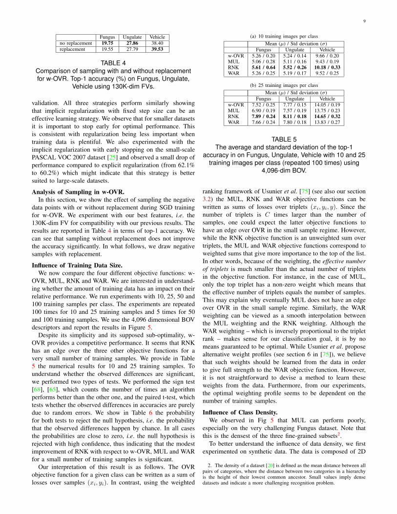
validation. All three strategies perform similarly showing

that implicit regularization with fixed step size can be an

effective learning strategy. We observe that for smaller datasets

it is important to stop early for optimal performance. This

is consistent with regularization being less important when

training data is plentiful. We also experimented with the

implicit regularization with early stopping on the small-scale

PASCAL VOC 2007 dataset [25] and observed a small drop of

performance compared to explicit regularization (from 62.1%

to 60.2%) which might indicate that this strategy is better

suited to large-scale datasets.

Analysis of Sampling in w-OVR.

In this section, we show the effect of sampling the negative

data points with or without replacement during SGD training

for w-OVR. We experiment with our best features, i.e. the

130K-dim FV for compatibility with our previous results. The

results are reported in Table 4 in terms of top-1 accuracy. We

can see that sampling without replacement does not improve

the accuracy significantly. In what follows, we draw negative

samples with replacement.

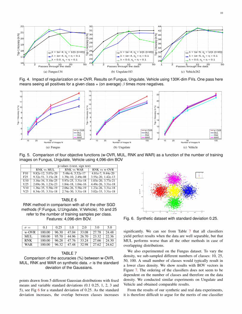
Influence of Training Data Size.

We now compare the four different objective functions: w-

OVR, MUL, RNK and WAR. We are interested in understand-

ing whether the amount of training data has an impact on their

relative performance. We run experiments with 10, 25, 50 and

100 training samples per class. The experiments are repeated

100 times for 10 and 25 training samples and 5 times for 50

and 100 training samples. We use the 4,096 dimensional BOV

descriptors and report the results in Figure 5.

Despite its simplicity and its supposed sub-optimality, w-

OVR provides a competitive performance. It seems that RNK

has an edge over the three other objective functions for a

very small number of training samples. We provide in Table

5 the numerical results for 10 and 25 training samples. To

understand whether the observed differences are significant,

we performed two types of tests. We performed the sign test

[68], [65], which counts the number of times an algorithm

performs better than the other one, and the paired t-test, which

tests whether the observed differences in accuracies are purely

due to random errors. We show in Table 6 the probability

for both tests to reject the null hypothesis, i.e. the probability

that the observed differences happen by chance. In all cases

the probabilities are close to zero, i.e. the null hypothesis is

rejected with high confidence, thus indicating that the modest

improvement of RNK with respect to w-OVR, MUL and WAR

for a small number of training samples is significant.

Our interpretation of this result is as follows. The OVR

objective function for a given class can be written as a sum of

losses over samples (xi, yi). In contrast, using the weighted

(a) 10 training images per class

Mean (µ) / Std deviation (σ)

Fungus Ungulate Vehicle

w-OVR 5.26 / 0.20 5.24 / 0.14 9.66 / 0.20MUL 5.06 / 0.28 5.11 / 0.16 9.43 / 0.19RNK 5.61 / 0.64 5.52 / 0.26 10.18 / 0.33

WAR 5.26 / 0.25 5.19 / 0.17 9.52 / 0.25

(b) 25 training images per class

Mean (µ) / Std deviation (σ)

Fungus Ungulate Vehicle

w-OVR 7.52 / 0.25 7.77 / 0.15 14.05 / 0.19MUL 6.90 / 0.19 7.57 / 0.19 13.75 / 0.23RNK 7.89 / 0.24 8.11 / 0.18 14.65 / 0.32

WAR 7.66 / 0.24 7.80 / 0.18 13.83 / 0.27

TABLE 5

The average and standard deviation of the top-1

accuracy in on Fungus, Ungulate, Vehicle with 10 and 25

training images per class (repeated 100 times) using

4,096-dim BOV.

ranking framework of Usunier et al. [75] (see also our section

3.2) the MUL, RNK and WAR objective functions can be

written as sums of losses over triplets (xi, yi, y). Since the

number of triplets is C times larger than the number of

samples, one could expect the latter objective functions to

have an edge over OVR in the small sample regime. However,

while the RNK objective function is an unweighted sum over

triplets, the MUL and WAR objective functions correspond to

weighted sums that give more importance to the top of the list.

In other words, because of the weighting, the effective number

of triplets is much smaller than the actual number of triplets

in the objective function. For instance, in the case of MUL,

only the top triplet has a non-zero weight which means that

the effective number of triplets equals the number of samples.

This may explain why eventually MUL does not have an edge

over OVR in the small sample regime. Similarly, the WAR

weighting can be viewed as a smooth interpolation between

the MUL weighting and the RNK weighting. Although the

WAR weighting – which is inversely proportional to the triplet

rank – makes sense for our classification goal, it is by no

means guaranteed to be optimal. While Usunier et al. propose

alternative weight profiles (see section 6 in [75]), we believe

that such weights should be learned from the data in order

to give full strength to the WAR objective function. However,

it is not straightforward to devise a method to learn these

weights from the data. Furthermore, from our experiments,

the optimal weighting profile seems to be dependent on the

number of training samples.

Influence of Class Density.

We observed in Fig 5 that MUL can perform poorly,

especially on the very challenging Fungus dataset. Note that

this is the densest of the three fine-grained subsets2.

To better understand the influence of data density, we first

experimented on synthetic data. The data is composed of 2D

2. The density of a dataset [20] is defined as the mean distance between allpairs of categories, where the distance between two categories in a hierarchyis the height of their lowest common ancestor. Small values imply densedatasets and indicate a more challenging recognition problem.

10

1 2 5 10 20 5016

17

18

19

20

21

22

Passes through the data

Top−

1 Ac

cura

cy (i

n %

)

λ = 1e−4, ηt = 1/(λ (t+t0))

λ = 1e−4, ηt = η = 0.1

λ = 0.0, ηt = η = 0.1

(a) Fungus134

1 2 5 10 20 5023

24

25

26

27

28

29

30

31

32

Passes through the data

Top−

1 Ac

cura

cy (i

n %

)

λ = 1e−4, ηt = 1/(λ (t+t0))

λ = 1e−4, ηt = η = 0.1

λ = 0.0, ηt = η = 0.1

(b) Ungulate183

1 2 5 10 20 50

28

30

32

34

36

38

40

42

44

Passes through the data

Top−

1 Ac

cura

cy (i

n %

)

λ = 1e−5, ηt = 1/(λ (t+t0))

λ = 1e−5, ηt = η = 0.1

λ = 0.0, ηt = η = 0.1

(c) Vehicle262

Fig. 4. Impact of regularization on w-OVR. Results on Fungus, Ungulate, Vehicle using 130K-dim FVs. One pass here

means seeing all positives for a given class + (on average) β times more negatives.

10 25 50 1004

5

6

7

8

9

10

11

12

13

Influence of number of training images with all SGD methods on Fungus

Number of Images N

Top−1Accuracy

(in%)

w−OVRMULRNKWAR

(a) Fungus

10 25 50 1004

5

6

7

8

9

10

11

12

13

14

15

Influence of number of training images with all SGD methods on Ungulate

Number of Images N

To

p−

1A

ccu

racy

(in

%)

w−OVRMULRNKWAR

(b) Ungulate

10 25 50 1008

10

12

14

16

18

20

22

Influence of number of training images with all SGD methods on Vehicle

Number of Images N

Top−1Accuracy

(in%)

w−OVRMULRNKWAR

(c) Vehicle

Fig. 5. Comparison of four objective functions (w-OVR, MUL, RNK and WAR) as a function of the number of training

images on Fungus, Ungulate, Vehicle using 4,096-dim BOV

p-values (t-test, sign test)

RNK vs MUL RNK vs WAR RNK vs w-OVR

F10 9.82e-12, 5.07e-20 5.48e-6, 5.52e-17 4.81e-7, 9.44e-20F25 9.32e-51, 3.15e-28 1.39e-10, 2.49e-08 3.55e-20, 1.42e-13

U10 3.16e-34, 5.10e-25 5.97e-25, 3.31e-18 1.03e-20, 3.77e-21U25 2.69e-36, 1.23e-23 1.84e-18, 1.04e-16 4.49e-26, 3.31e-18

V10 1.36e-35, 5.58e-19 2.06e-26, 5.58e-19 1.23e-26, 3.31e-18V25 8.34e-35, 3.31e-18 2.74e-30, 3.31e-18 3.02e-33, 3.31e-18

TABLE 6

RNK method in comparison with all of the other SGD

methods (F:Fungus, U:Ungulate, V:Vehicle). 10 and 25

refer to the number of training samples per class.

Features: 4,096-dim BOV.

σ = 0.1 0.25 1.0 2.0 3.0 5.0

w-OVR 100.00 96.30 47.04 33.08 27.78 24.48

MUL 100.00 95.70 44.96 26.70 23.32 22.36

RNK 100.00 96.28 47.76 33.24 27.66 24.30

WAR 100.00 96.32 47.48 32.98 27.62 24.62

TABLE 7

Comparison of the accuracies (%) between w-OVR,

MUL, RNK and WAR on synthetic data. σ is the standard

deviation of the Gaussians.

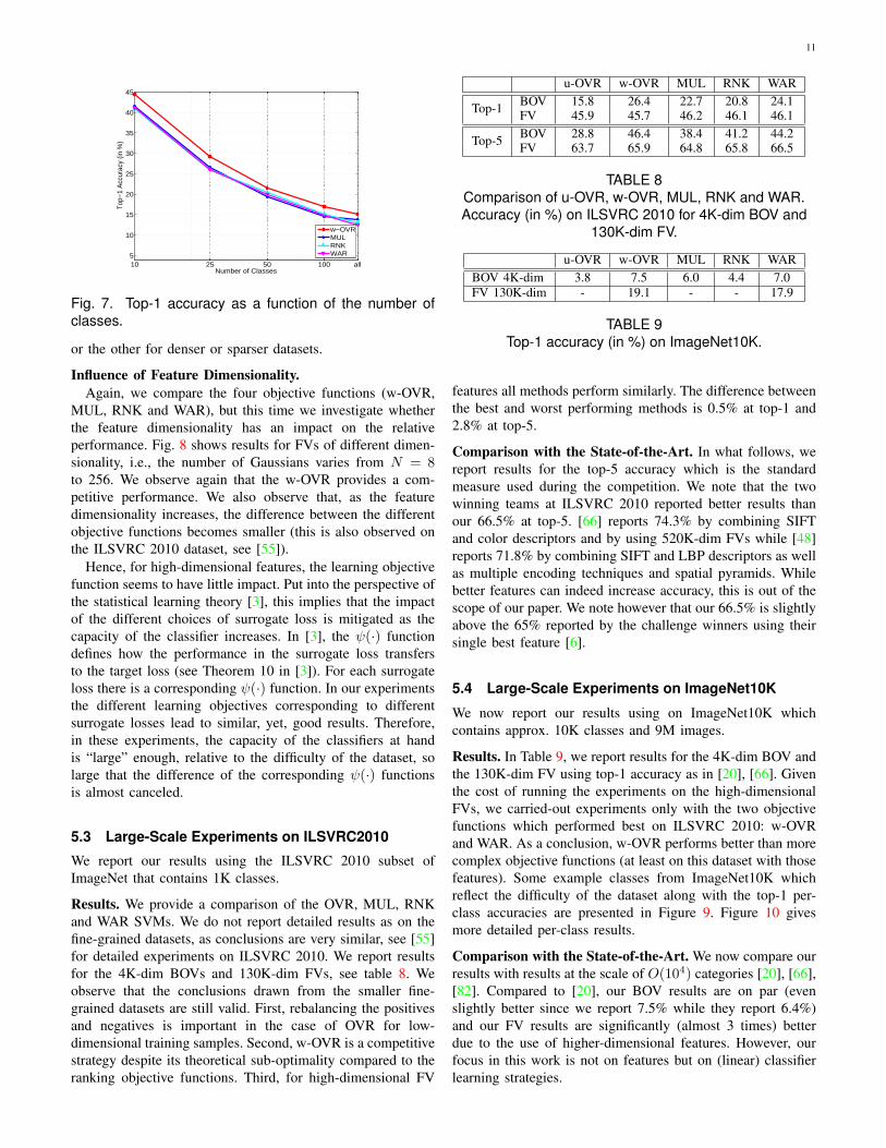
points drawn from 5 different Gaussian distributions with fixed

means and variable standard deviations (0.1 0.25, 1, 2, 3 and

5), see Fig 6 for a standard deviation of 0.25. As the standard

deviation increases, the overlap between classes increases

Fig. 6. Synthetic dataset with standard deviation 0.25.

significantly. We can see from Table 7 that all classifiers

yield perfect results when the data are well separable, but that

MUL performs worse than all the other methods in case of

overlapping distributions.

We also experimented on the Fungus dataset. To vary the

density, we sub-sampled different numbers of classes: 10, 25,

50, 100. A small number of classes would typically result in

a lower class density. We show results with BOV vectors in

Figure 7. The ordering of the classifiers does not seem to be

dependent on the number of classes and therefore on the data

density. We conducted similar experiments on Ungulate and

Vehicle and obtained comparable results.

From the results of our synthetic and real data experiments,

it is therefore difficult to argue for the merits of one classifier

11

10 25 50 100 all5

10

15

20

25

30

35

40

45

Number of Classes

Top−

1 A

ccur

acy

(in %

)

w−OVRMULRNKWAR

Fig. 7. Top-1 accuracy as a function of the number of

classes.

or the other for denser or sparser datasets.

Influence of Feature Dimensionality.

Again, we compare the four objective functions (w-OVR,

MUL, RNK and WAR), but this time we investigate whether

the feature dimensionality has an impact on the relative

performance. Fig. 8 shows results for FVs of different dimen-

sionality, i.e., the number of Gaussians varies from N = 8to 256. We observe again that the w-OVR provides a com-

petitive performance. We also observe that, as the feature

dimensionality increases, the difference between the different

objective functions becomes smaller (this is also observed on

the ILSVRC 2010 dataset, see [55]).

Hence, for high-dimensional features, the learning objective

function seems to have little impact. Put into the perspective of

the statistical learning theory [3], this implies that the impact

of the different choices of surrogate loss is mitigated as the

capacity of the classifier increases. In [3], the ψ(·) function

defines how the performance in the surrogate loss transfers

to the target loss (see Theorem 10 in [3]). For each surrogate

loss there is a corresponding ψ(·) function. In our experiments

the different learning objectives corresponding to different

surrogate losses lead to similar, yet, good results. Therefore,

in these experiments, the capacity of the classifiers at hand

is “large” enough, relative to the difficulty of the dataset, so

large that the difference of the corresponding ψ(·) functions

is almost canceled.

5.3 Large-Scale Experiments on ILSVRC2010

We report our results using the ILSVRC 2010 subset of

ImageNet that contains 1K classes.

Results. We provide a comparison of the OVR, MUL, RNK

and WAR SVMs. We do not report detailed results as on the

fine-grained datasets, as conclusions are very similar, see [55]

for detailed experiments on ILSVRC 2010. We report results

for the 4K-dim BOVs and 130K-dim FVs, see table 8. We

observe that the conclusions drawn from the smaller fine-

grained datasets are still valid. First, rebalancing the positives

and negatives is important in the case of OVR for low-

dimensional training samples. Second, w-OVR is a competitive

strategy despite its theoretical sub-optimality compared to the

ranking objective functions. Third, for high-dimensional FV

u-OVR w-OVR MUL RNK WAR

Top-1BOV 15.8 26.4 22.7 20.8 24.1FV 45.9 45.7 46.2 46.1 46.1

Top-5BOV 28.8 46.4 38.4 41.2 44.2FV 63.7 65.9 64.8 65.8 66.5

TABLE 8

Comparison of u-OVR, w-OVR, MUL, RNK and WAR.

Accuracy (in %) on ILSVRC 2010 for 4K-dim BOV and

130K-dim FV.

u-OVR w-OVR MUL RNK WAR

BOV 4K-dim 3.8 7.5 6.0 4.4 7.0

FV 130K-dim - 19.1 - - 17.9

TABLE 9

Top-1 accuracy (in %) on ImageNet10K.

features all methods perform similarly. The difference between

the best and worst performing methods is 0.5% at top-1 and

2.8% at top-5.

Comparison with the State-of-the-Art. In what follows, we

report results for the top-5 accuracy which is the standard

measure used during the competition. We note that the two

winning teams at ILSVRC 2010 reported better results than

our 66.5% at top-5. [66] reports 74.3% by combining SIFT

and color descriptors and by using 520K-dim FVs while [48]

reports 71.8% by combining SIFT and LBP descriptors as well

as multiple encoding techniques and spatial pyramids. While

better features can indeed increase accuracy, this is out of the

scope of our paper. We note however that our 66.5% is slightly

above the 65% reported by the challenge winners using their

single best feature [6].

5.4 Large-Scale Experiments on ImageNet10K

We now report our results using on ImageNet10K which

contains approx. 10K classes and 9M images.

Results. In Table 9, we report results for the 4K-dim BOV and

the 130K-dim FV using top-1 accuracy as in [20], [66]. Given

the cost of running the experiments on the high-dimensional

FVs, we carried-out experiments only with the two objective

functions which performed best on ILSVRC 2010: w-OVR

and WAR. As a conclusion, w-OVR performs better than more

complex objective functions (at least on this dataset with those

features). Some example classes from ImageNet10K which

reflect the difficulty of the dataset along with the top-1 per-

class accuracies are presented in Figure 9. Figure 10 gives

more detailed per-class results.

Comparison with the State-of-the-Art. We now compare our

results with results at the scale of O(104) categories [20], [66],

[82]. Compared to [20], our BOV results are on par (even

slightly better since we report 7.5% while they report 6.4%)

and our FV results are significantly (almost 3 times) better

due to the use of higher-dimensional features. However, our

focus in this work is not on features but on (linear) classifier

learning strategies.

12

8 16 32 64 128 25610

11

12

13

14

15

16

17

18

19

20

21

Number of Gaussians N

Top−

1 A

ccur

acy

(in %

)

w−OVRMULRNKWAR

(a) Fungus

8 16 32 64 128 25610

12

14

16

18

20

22

24

26

28

30

32

Number of Gaussians N

Top−

1 A

ccur

acy

(in %

)

w−OVRMULRNKWAR

(b) Ungulate

8 16 32 64 128 256

26

28

30

32

34

36

38

40

42

Number of Gaussians N

Top−

1 A

ccur

acy

(in %

)

w−OVRMULRNKWAR

(c) Vehicle

Fig. 8. Comparison of Top-1 Accuracy between the w-OVR, MUL, RNK and WAR SVMs as a function of the number

of Gaussians used to compute the FV (i.e. as a function of the FV dimensionality). No spatial pyramids were used to

speed-up these experiments.

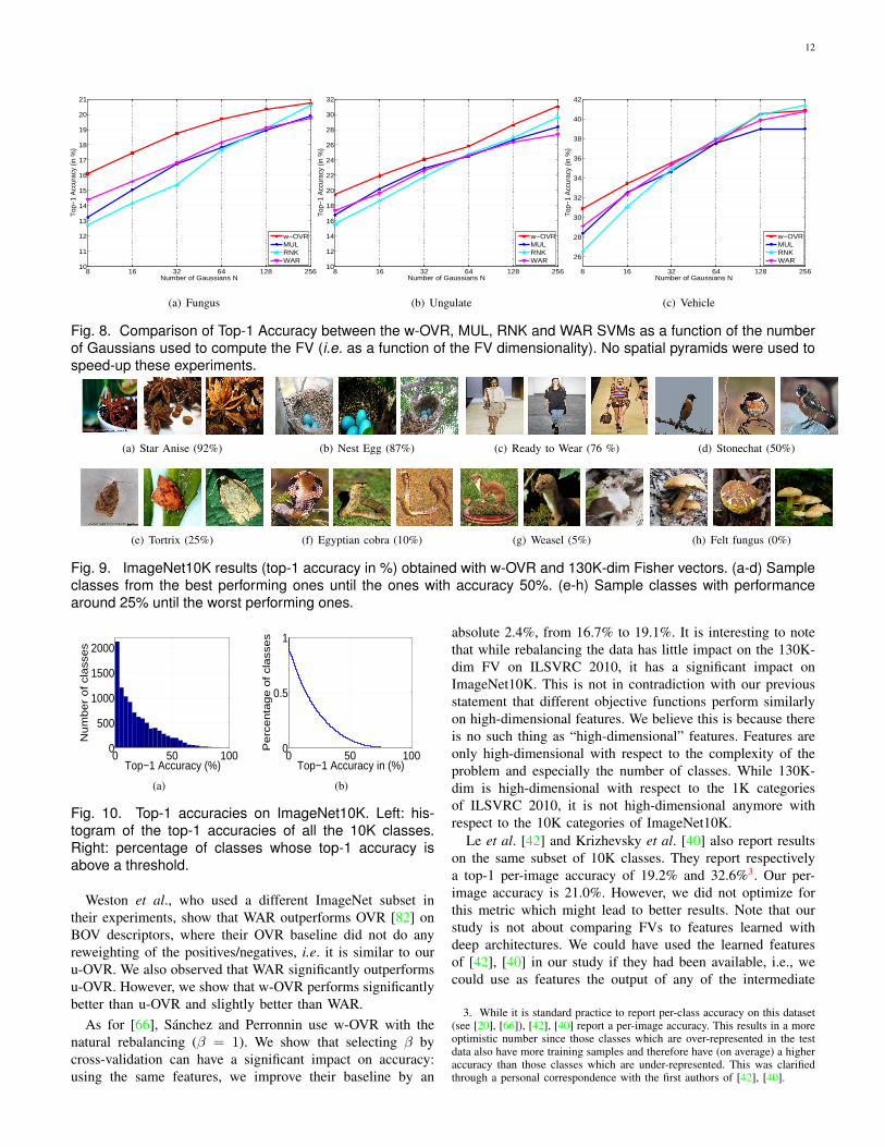
(a) Star Anise (92%) (b) Nest Egg (87%) (c) Ready to Wear (76 %) (d) Stonechat (50%)

(e) Tortrix (25%) (f) Egyptian cobra (10%) (g) Weasel (5%) (h) Felt fungus (0%)

Fig. 9. ImageNet10K results (top-1 accuracy in %) obtained with w-OVR and 130K-dim Fisher vectors. (a-d) Sample

classes from the best performing ones until the ones with accuracy 50%. (e-h) Sample classes with performance

around 25% until the worst performing ones.

0 50 1000

500

1000

1500

2000

Top−1 Accuracy (%)

Nu

mb

er

of cl

ass

es

(a)

0 50 1000

0.5

1

Pe

rce

nta

ge

of cl

ass

es

Top−1 Accuracy in (%)

(b)

Fig. 10. Top-1 accuracies on ImageNet10K. Left: his-

togram of the top-1 accuracies of all the 10K classes.

Right: percentage of classes whose top-1 accuracy is

above a threshold.

Weston et al., who used a different ImageNet subset in

their experiments, show that WAR outperforms OVR [82] on

BOV descriptors, where their OVR baseline did not do any

reweighting of the positives/negatives, i.e. it is similar to our

u-OVR. We also observed that WAR significantly outperforms

u-OVR. However, we show that w-OVR performs significantly

better than u-OVR and slightly better than WAR.

As for [66], Sanchez and Perronnin use w-OVR with the

natural rebalancing (β = 1). We show that selecting β by

cross-validation can have a significant impact on accuracy:

using the same features, we improve their baseline by an

absolute 2.4%, from 16.7% to 19.1%. It is interesting to note

that while rebalancing the data has little impact on the 130K-

dim FV on ILSVRC 2010, it has a significant impact on

ImageNet10K. This is not in contradiction with our previous

statement that different objective functions perform similarly

on high-dimensional features. We believe this is because there

is no such thing as “high-dimensional” features. Features are

only high-dimensional with respect to the complexity of the

problem and especially the number of classes. While 130K-

dim is high-dimensional with respect to the 1K categories

of ILSVRC 2010, it is not high-dimensional anymore with

respect to the 10K categories of ImageNet10K.

Le et al. [42] and Krizhevsky et al. [40] also report results

on the same subset of 10K classes. They report respectively

a top-1 per-image accuracy of 19.2% and 32.6%3. Our per-

image accuracy is 21.0%. However, we did not optimize for

this metric which might lead to better results. Note that our

study is not about comparing FVs to features learned with

deep architectures. We could have used the learned features

of [42], [40] in our study if they had been available, i.e., we

could use as features the output of any of the intermediate

3. While it is standard practice to report per-class accuracy on this dataset(see [20], [66]), [42], [40] report a per-image accuracy. This results in a moreoptimistic number since those classes which are over-represented in the testdata also have more training samples and therefore have (on average) a higheraccuracy than those classes which are under-represented. This was clarifiedthrough a personal correspondence with the first authors of [42], [40].

13

layers.

Timing for ImageNet10K for 130K-dim FVs. For the com-

putation we used a small cluster of machines with 16 CPUs

and 32GB of RAM. The feature extraction step (including

SIFT description and FV computation) took approx. 250 CPU

days, the learning of the w-OVR SVM approx. 400 CPU days

and the learning of the WAR SVM approx. 500 CPU days.

Note that w-OVR performs slightly better than WAR and is

much easier to parallelize since the classifiers can be learned

independently.

6 CONCLUSION

In this work, we have studied visual classification on a large-

scale, i.e. when we have to deal with a large number of classes,

a large number of images and high dimensional features.

Two main conclusions have emerged from our work. The

first one is that, despite its theoretical suboptimality, one-vs-

rest is a very competitive training strategy to learn SVMs.

Furthermore, one-vs-rest SVMs are easy to implement and to

parallelize, e.g. by training the different classifiers on multiple

machines/cores. However, to obtain state-of-the-art results,

properly cross-validating the imbalance between positive and

negative samples is a must. The second major conclusion

is that stochastic training is very well suited to our large-

scale setting. Moreover simple strategies such as implicit

regularization with early stopping and fixed-step-size updates

work well in practice. Following these good practices, we were

able to improve the state-of-the-art on a large subset of 10K

classes and 9M images from 16.7% Top-1 accuracy to 19.1%.

Acknowledgements. The INRIA LEAR team acknowledges

financial support from the QUAERO project supported by

OSEO, the French State agency for innovation, the European

integrated project AXES, the ERC grant ALLEGRO and the

GARGANTUA project funded by the Mastodons program of

CNRS. The authors wish to warmly thank Matthijs Douze

and Mattis Paulin for providing a public implementation of

the online learning code described in this article.

REFERENCES

[1] E. L. Allwein, R. E. Schapire, and Y. Singer. Reducing multiclass tobinary: A unifying approach for margin classifiers. In ICML, 2000. 3

[2] B. Bai, J. Weston, D. Grangier, R. Collobert, O. Chapelle, and K. Wein-berger. Supervised semantic indexing. In CIKM, 2009. 6

[3] P. L. Bartlett, M. I. Jordan, and J. D. McAuliffe. Convexity, classifica-tion, and risk bounds. In NIPS, 2003. 11

[4] S. Bengio, J. Weston, and D. Grangier. Label embedding trees for largemulti-class tasks. In NIPS, 2010. 1, 3

[5] Y. Bengio, A. Courville, and P. Vincent. Representation learning: areview and new perspectives. 3

[6] A. Berg, J. Deng, and L. Fei-Fei. ILSVRC 2010. http://www.image-net.org/challenges/LSVRC/2010/index. 1, 6, 11

[7] A. Bergamo, L. Torresani, and A. Fitzgibbon. PICODES: Learning acompact code for novel-category recognition. In NIPS, 2011. 3

[8] A. Beygelzimer, V. Dani, T. P. Hayes, J. Langford, and B. Zadrozny.Error limiting reductions between classification tasks. In ICML, 2005.3

[9] A. Bordes, L. Bottou, P. Gallinari, and J. Weston. Solving multiclasssupport vector machines with LaRank. In ICML, 2007. 1

[10] L. Bottou. SGD. http://leon.bottou.org/projects/sgd. 4, 5, 8[11] L. Bottou and O. Bousquet. The tradeoffs of large scale learning. In

NIPS, 2007. 1, 5, 7

[12] Y.-L. Bourreau, F. Bach, Y. LeCun, and J. Ponce. Learning mid-levelfeatures for recognition. In CVPR, 2010. 2

[13] G. Burghouts and J.-M. Geusebroek. Performance evaluation of localcolour invariants. CVIU, 2009. 2

[14] P. K. Chan and S. J. Stolfo. On the accuracy of meta-learning forscalable data mining. JIIS, 1997. 3

[15] C.-C. Chang and C.-J. Lin. LIBSVM: A library for support vectormachines. ACM TIST, 2011. Software available at http://www.csie.ntu.edu.tw/∼cjlin/libsvm. 4, 7

[16] K. Chatfield, V. Lempitsky, A. Vedaldi, and A. Zisserman. The devilis in the details: an evaluation of recent feature encoding methods. InBMVC, 2011. 3, 7

[17] K. Crammer and Y. Singer. On the algorithmic implementation ofmulticlass kernel-based vector machines. JMLR, 2002. 1, 3, 4

[18] G. Csurka, C. Dance, L. Fan, J. Willamowski, and C. Bray. Visualcategorization with bags of keypoints. In ECCV SLCV workshop, 2004.2

[19] J. Dean, G. Corrado, R. Monga, M. Devin, Q. Le, M. Mao, M. Ranzato,A. Senior, P. Tucker, K. Yang, and A. Ng. Large scale distributed deepnetworks. In NIPS, 2012. 3

[20] J. Deng, A. Berg, K. Li, and L. Fei-Fei. What does classifying morethan 10,000 image categories tell us? In ECCV, 2010. 1, 3, 6, 7, 9, 11,12

[21] J. Deng, W. Dong, R. Socher, L.-J. Li, K. Li, and L. Fei-Fei. Imagenet:A large-scale hierarchical image database. In CVPR, 2009. 1, 2

[22] J. Deng, S. Satheesh, A. Berg, and L. Fei-Fei. Fast and balanced:efficient label tree learning for large scale object recognition. In NIPS,2011. 1

[23] T. Deselaers and V. Ferrari. Visual and semantic similarity in imagenet.In CVPR, 2011. 7

[24] T. G. Dietterich and G. Bakiri. Solving multiclass learning problemsvia error-correcting output codes. JAIR, 1995. 3

[25] M. Everingham, L. V. Gool, C. Williams, J. Winn, and A. Zisserman.The pascal visual object classes (VOC) challenge. IJCV, 2010. 2, 9

[26] R.-E. Fan, K.-W. Chang, C.-J. Hsieh, X.-R. Wang, and C.-J. Lin.LIBLINEAR: A library for large linear classification. JMLR, 2008. 7

[27] J. Farquhar, S. Szedmak, H. Meng, and J. Shawe-Taylor. Improvingbag-of-keypoints image categorisation. Technical report, University ofSouthampton, 2005. 2

[28] V. Franc and S. Sonnenburg. Optimized cutting plane algorithm forsupport vector machines. In ICML, 2008. 4

[29] T. Gao and D. Koller. Discriminative learning of relaxed hierarchy forlarge-scale visual recognition. In ICCV, 2011. 3

[30] J. Gehrke, R. Ramakrishnan, and V. Ganti. Rainforest - a frameworkfor fast decision tree construction of large datasets. DMKD, 2000. 3

[31] Y. Gong and S. Lazebnik. Comparing data-dependent and data-independent embeddings for classification and ranking of internet im-ages. In CVPR, 2011. 2

[32] D. Grangier, F. Monay, and S. Bengio. A discriminative approach forthe retrieval of images from text queries. In ECML, 2006. 3

[33] C.-J. Hsieh, K.-W. Chang, C.-J. Lin, S. S. Keerthi, and S. Sundararajan.A dual coordinate descent method for large-scale linear svm. In ICML,2008. 4

[34] K. Jarrett, K. Kavukcuoglu, M. Ranzato, and Y. LeCun. What is thebest multi-stage architecture for object recognition? In ICCV, 2009. 3

[35] H. Jegou, M. Douze, and C. Schmid. Product quantization for nearestneighbor search. IEEE TPAMI, 2011. 3, 7

[36] H. Jegou, F. Perronnin, M. Douze, J. Sanchez, P. Perez, and C. Schmid.Aggregating local image descriptors into compact codes. IEEE TPAMI,accepted. 3

[37] T. Joachims. Making large-scale support vector machine learningpractical. In Advances in kernel methods. 1999. 4

[38] T. Joachims. Optimizing search engines using clickthrough data. InACM SIGKDD, pages 133–142. ACM, 2002. 1, 3, 4

[39] T. Joachims. Training linear svms in linear time. In ACM SIGKDD,2006. 7

[40] A. Krizhevsky, I. Sutskever, and G. Hinton. Image classification withdeep convolutional neural networks. In NIPS, 2012. 2, 3, 12

[41] S. Lazebnik, C. Schmid, and J. Ponce. Beyond bags of features: Spatialpyramid matching for recognizing natural scene categories. In CVPR,2006. 2

[42] Q. Le, M. Ranzato, R. Monga, M. Devin, K. Chen, G. Corrado, J. Dean,and A. Ng. Building high-level features using large scale unsupervisedlearning. In ICML, 2012. 2, 3, 12

[43] Y. LeCun, B. Boser, J. Denker, D. Henderson, R. Howard, W. Hubbard,and L. Jackel. Handwritten digit recognition with a back-propagationnetwork. In NIPS, 1989. 3

[44] Y. LeCun, L. Bottou, G. Orr, and K. Muller. Efficient backprop. InNeural Networks: Tricks of the trade. Springer, 1998. 1

[45] Y. LeCun, F. Huang, and L. Bottou. Learning methods for generic object

14

recognition with invariance to pose and lighting. In CVPR, 2004. 3[46] T. Lee, Y. Lin, and G. Wahba. Multicategory support vector machines:

Theory and application to the classification of microarray data andsatellite radiance data. JASA, 2004. 3

[47] L. Li, H. Su, E. Xing, and L. Fei-Fei. Object bank: A high-level imagerepresentation for scene classification and semantic feature sparsifica-tion. In NIPS, 2010. 3

[48] Y. Lin, F. Lv, S. Zhu, M. Yang, T. Cour, K. Yu, L. Cao, and T. Huang.Large-scale image classification: Fast feature extraction and SVM train-ing. In CVPR, 2011. 1, 2, 3, 5, 11

[49] Y. Lin, F. Lv, S. Zhu, K. Yu, M. Yang, and T. Cour. Large-scale imageclassification: fast feature extraction and svm training. In CVPR, 2011.3

[50] D. G. Lowe. Distinctive image features from scale-invariant keypoints.IJCV, 2004. 2, 7

[51] S. Maji and A. Berg. Max-margin additive classifiers for detection. InICCV, 2009. 2

[52] M. Marszalek and C. Schmid. Constructing category hierarchies forvisual recognition. In ECCV, 2008. 3

[53] M. Mehta, R. Agrawal, and J. Rissanen. Sliq: A fast scalable classifierfor data mining. In EDBT, 1996. 3

[54] S. Nowozin and C. Lampert. Structured Learning and Prediction in

Computer Vision. Foundations and Trends in Computer Graphics andVision, 2011. 1

[55] F. Perronnin, Z. Akata, Z. Harchaoui, and C. Schmid. Towards goodpractice in large-scale learning for image classification. In CVPR, 2012.2, 11

[56] F. Perronnin and C. Dance. Fisher kernels on visual vocabularies forimage categorization. In CVPR, 2007. 2

[57] F. Perronnin, J. Sanchez, and Y. Liu. Large-scale image categorizationwith explicit data embedding. In CVPR, 2010. 2, 3, 5

[58] F. Perronnin, J. Sanchez, and T. Mensink. Improving the Fisher kernelfor large-scale image classification. In ECCV, 2010. 1, 5

[59] J. C. Platt. Fast training of support vector machines using sequentialminimal optimization. In Advances in kernel methods. 1999. 3

[60] M. Rastegari, C. Fang, and L. Torresani. Scalable object-class retrievalwith approximate and top-k ranking. In ICCV, 2011. 3

[61] R. Rifkin and A. Klautau. In defense of one-vs-all classification. JMLR,2004. 3

[62] M. Rohrbach, M. Stark, and B.Schiele. Evaluating knowledge transferand zero-shot learning in a large-scale setting. In CVPR, 2011. 1, 3, 5

[63] L. Rokach and O. Maimon. Top-down induction of decision treesclassifiers - a survey. IEEE TSMC, 2005. 3

[64] B. C. Russell, A. Torralba, K. P. Murphy, and W. T. Freeman. Labelme:A database and web-based tool for image annotation. IJCV, 2008. 2

[65] S. L. Salzberg. On comparing classifiers: Pitfalls toavoid and arecommended approach. DMKD. 9

[66] J. Sanchez and F. Perronnin. High-dimensional signature compressionfor large-scale image classification. In CVPR, 2011. 1, 3, 5, 6, 7, 11,12

[67] S. Shalev-Shwartz, Y. Singer, and N. Srebro. Pegasos: Primal estimatesub-gradient solver for SVM. In ICML, 2007. 1, 4, 5, 7, 8

[68] D. J. Sheskin. Handbook of Parametric and Nonparametric Statistical

Procedures. Chapman & Hall/CRC, 4 edition, 2007. 9[69] J. Sivic and A. Zisserman. Video google: A text retrieval approach to

object matching in videos. In ICCV, 2003. 2[70] D. Tao, X. Tang, X. Li, and X. Wu. Asymmetric bagging and random

subspace for support vector machines-based relevance feedback in imageretrieval. IEEE Trans. Pattern Anal. Mach. Intell., 28(7), July 2006. 7

[71] A. Tewari and P. L. Bartlett. On the Consistency of MulticlassClassification Methods. JMLR, 2007. 3, 4

[72] A. Torralba, R. Fergus, and W. Freeman. 80 million tiny images: a largedataset for non-parametric object and scene recognition. IEEE TPAMI,2008. 1, 2, 3

[73] L. Torresani, M. Szummer, and A. Fitzgibbon. Efficient object categoryrecognition using classemes. In ECCV, 2010. 3

[74] I. Tsochantaridis, T. Joachims, T. Hofmann, and Y. Altun. Large marginmethods for structured and interdependent output variables. JMLR, 2005.4

[75] N. Usunier, D. Buffoni, and P. Gallinari. Ranking with ordered weightedpairwise classification. In ICML, 2009. 1, 3, 4, 5, 9

[76] J. C. van Gemert, C. J. Veenman, A. W. M. Smeulders, and J. M.Geusebroek. Visual word ambiguity. IEEE TPAMI, 2010. 2

[77] A. Vedaldi and A. Zisserman. Efficient additive kernels via explicitfeature maps. In CVPR, 2010. 2

[78] A. Vedaldi and A. Zisserman. Sparse kernel approximations for efficientclassification and detection. In CVPR, 2012. 3

[79] V. Vural and J. G. Dy. A hierarchical method for multi-class supportvector machines. In ICML, 2004. 3

[80] G. Wang, D. Hoiem, and D. Forsyth. Learning image similarity from

Flickr groups using stochastic intersection kernel machines. In ICCV,2009. 1, 3

[81] J. Wang, J. Yang, K. Yu, F. Lv, T. Huang, and Y. Gong. Locality-constrained linear coding for image classification. In CVPR, 2010. 2

[82] J. Weston, S. Bengio, and N. Usunier. Large scale image annotation:Learning to rank with joint word-image embeddings. ECML, 2010. 1,3, 5, 6, 7, 11, 12

[83] J. Weston, S. Bengio, and N. Usunier. Wsabie: Scaling up to largevocabulary image annotation. In IJCAI, 2011. 3

[84] J. Weston and C. Watkins. Multi-class support vector machines.Technical report, Department of Computer Science, Royal Holloway,University of London, 1998. 4

[85] J. Weston and C. Watkins. Support vector machines for multi-classpattern recognition. In ESANN, 1999. 3

[86] J. Xu, T. Liu, M. Lu, H. Li, and W. Ma. Directly optimizing evaluationmeasures in learning to rank. In SIGIR, 2008. 1, 5

[87] J. Yang, K. Yu, Y. Gong, and T. S. Huang. Linear spatial pyramidmatching using sparse coding for image classification. In CVPR, 2009.2

[88] Y. Yue, T. Finley, F. Radlinski, and T. Joachims. A support vectormethod for optimizing average precision. In SIGIR, 2007. 1, 5

[89] B. Zhao, L. Fei-Fei, and E. Xing. Large-scale category structure awareimage categorization. In NIPS, 2011. 1

[90] Z. Zhou, K. Yu, T. Zhang, and T. Huang. Image classification usingsuper-vector coding of local image descriptors. In ECCV, 2010. 3

Zeynep Akata received her MSc degree in 2010from the Media Informatics department of RWTHAachen University, Germany. She is currentlyworking on her PhD in the CV team of the XeroxResearch Centre Europe and the LEAR team atINRIA Grenoble. She is working on image classi-fication for large scale datasets and is interestedin learning methods for classification. She is astudent member of IEEE.

Florent Perronnin holds an Engineering de-gree from the Ecole Nationale Superieure desTelecommunications and a Ph.D. degree fromthe Ecole Polytechnique Federale de Lausanne.In 2005, he joined the Xerox Research CentreEurope in Grenoble where he currently managesthe CV team. His main interests are in the ap-plication of machine learning to computer visiontasks such as image classification, retrieval orsegmentation.

Zaid Harchaoui graduated from the Ecole Na-tionale Superieure des Mines, France, in 2004,and obtained his Ph.D. degree from ParisTech,Paris, France. Since 2010, he is a permanentresearcher in the LEAR team, INRIA Grenoble,France. His research interests include statisticalmachine learning, kernel-based methods, signalprocessing, and computer vision.

Cordelia Schmid holds a M.S. degree in com-puter science from the University of Karlsruheand a doctorate from the Institut National Poly-technique de Grenoble. She is a research di-rector at INRIA Grenoble where she directs theLEAR team. In 2006, she was awarded theLonguet-Higgins prize for fundamental contribu-tions in computer vision that have withstood thetest of time. In 2012, she obtained an ERCadvanced grant for ”Active large-scale learningfor visual recognition”. She is a fellow of IEEE.