Good Mine, Bad Mine: Natural Resource Heterogeneity and ...

7284 2018

September 2018

Good Mine, Bad Mine: Natural Resource Heterogeneity and Dutch Disease in Indonesia Paul Pelzl, Steven Poelhekke

Impressum:

CESifo Working Papers ISSN 2364‐1428 (electronic version) Publisher and distributor: Munich Society for the Promotion of Economic Research ‐ CESifo GmbH The international platform of Ludwigs‐Maximilians University’s Center for Economic Studies and the ifo Institute Poschingerstr. 5, 81679 Munich, Germany Telephone +49 (0)89 2180‐2740, Telefax +49 (0)89 2180‐17845, email [email protected] Editors: Clemens Fuest, Oliver Falck, Jasmin Gröschl www.cesifo‐group.org/wp An electronic version of the paper may be downloaded ∙ from the SSRN website: www.SSRN.com ∙ from the RePEc website: www.RePEc.org ∙ from the CESifo website: www.CESifo‐group.org/wp

CESifo Working Paper No. 7284 Category 9: Resource and Environment Economics

Good Mine, Bad Mine: Natural Resource Heterogeneity and Dutch Disease in Indonesia

Abstract We analyse the local effect of exogenous shocks to the value of mineral deposits at the district level in Indonesia using a panel of manufacturing plants. To the best of our knowledge, we are the first to model and estimate the effect of heterogeneity in natural resource extraction methods. We find that in areas where mineral extraction is relatively capital-intensive, mining booms cause virtually no upward pressure on manufacturing earnings per worker, and both producers of traded and local goods benefit from mining booms in terms of employment. In contrast, labour-intensive mining booms drive up local manufacturing wages such that producers of traded goods reduce employment. This source of heterogeneity helps to explain the mixed evidence for `Dutch disease' effects in the literature. In addition, we find no evidence that fiscal revenue sharing between sub-national districts leads to any spillovers.

JEL-Codes: L160; L720; O120; O130; Q300.

Keywords: dutch disease, natural resources, mining, labour intensity, Indonesia.

Paul Pelzl Vrije Universiteit Amsterdam

School of Business and Economics De Boelelaan 1105

The Netherlands – 1081 HV, Amsterdam [email protected]

Steven Poelhekke* Vrije Universiteit Amsterdam

School of Business and Economics De Boelelaan 1105

The Netherlands – 1081 HV, Amsterdam [email protected]

*corresponding author September 17, 2018 We thank Peter Lanjouw, Julian Emani Namini, Beata Javorcik, Massimiliano Cali, Dave Donaldson, Ralph de Haas, Aysil Emirmahmutoglu, Albert Jan Hummel, Andreas Ferrara, seminar participants at the Tinbergen Institute Amsterdam, Vrije Universiteit Amsterdam and Oesterreichische Nationalbank as well as conference participants at the CAED 2017 in Seoul, the 16th EUDN PhD Workshop on Development Economics in Wageningen and the 10th FIW conference in Vienna for helpful comments. All errors are our own. Further, we thank Beata Javorcik, Hengky Kurniawan and Menno Pradhan for providing data for this project, and Mark van der Harst for excellent research assistance.

1 Introduction

Wealth in non-renewable natural resources (such as solid minerals and oil & gas) does not always lead to

sustained economic development. This observation has long inspired a debate on the existence of a ‘Dutch

disease’ (Van Wijnbergen, 1984) or even a seemingly incurable ‘resource curse’ (Gelb, 1988). It is now gen-

erally accepted that negative outcomes are conditional on institutions and macroeconomic management of

subsoil wealth (Van der Ploeg, 2011). Recently, this literature has moved away from cross-country studies in

which endogeneity issues are harder to address and started to exploit within-country variation to minimize

the influence of confounding factors.1 This approach has contributed to our understanding of the underlying

mechanisms that may explain the negative aggregate correlation between resource wealth and growth. How-

ever, at the local level, and using detailed firm and household data for the US, several studies find positive

effects of a local natural resource boom, or at the least no evidence for crowding out of manufacturing firms

(Black et al., 2005; Michaels, 2011; Allcott and Keniston, 2018). For developing countries, the evidence is

more mixed and ranges from an increase in real income for households close to a large gold mine in Peru

(Aragon and Rud, 2013), to more conflict in Colombia (Dube and Vargas, 2013), localised negative traded-

sector employment effects in emerging markets (De Haas and Poelhekke, 2016), and an increase in municipal

government spending in Brazil that does not translate into higher public goods and services (Caselli and

Michaels, 2013).

The literature has typically identified these effects by exploiting geographic variation in natural resource

wealth and time variation in world prices or giant oil discoveries, but has not distinguished explicitly between

different resources or extraction techniques. We argue that the labour intensity of resource extraction can

reconcile positive and negative outcomes found in the literature. To the best of our knowledge, we are the

first to model and estimate the effect of heterogeneity in natural resource extraction methods. We analyse the

local effect of a booming natural resource sector within Indonesia, which is both a major producer of a variety

of natural resources that are scattered around the country, and has a large and exporting manufacturing

sector. Combining detailed manufacturing plant-level panel data with well- and deposit-level data, we find

that in areas where resource extraction is more capital-intensive, booms cause virtually no upward pressure

on manufacturing earnings per worker, and both producers of traded and local goods benefit from booms

in terms of employment. In the average mining district, the manufacturing sector increases employment

by 2 percent as local mineral prices double. In contrast, labour-intensive mining booms increase local

manufacturing wages by 6 percent such that producers of relatively traded goods reduce employment by

1 percent. From the perspective of manufacturing plants, mining booms can thus be good or bad. This

source of heterogeneity helps to explain why many studies that have focused on capital-intensive natural

resource extraction such as oil and gas do not find evidence for local ‘Dutch disease’ effects. The effect of

mining booms on local manufacturing is much larger than comparable effects in the US, but in Indonesia

due to minerals rather than oil and gas extraction. We do not find evidence that the reallocation between

1 As surveyed in Van der Ploeg and Poelhekke (2017) and Cust and Poelhekke (2015).

2

sectors and reduction in activity by traded goods producers leads to a reduction in total factor productivity.

In addition, we find that the effects of natural resource booms are local despite the government’s move to

decentralization and increased mineral revenue sharing across regions, which has not lead to a noticeable

spread of any benefits to non-extracting regions.

Our identification strategy is to correlate exogenous shocks to the value of local natural resources in Indonesia

discovered by 1990 with local manufacturing outcomes in subsequent years. Using deposit and well-level

data on the quantity, type and extraction method for each natural resource, we compute measures of initial

endowments of oil, gas, metals, and other minerals at the district level, and interact them with subsequent

exogenous world price shocks and an indicator that captures the extraction method’s labour-intensity. For

given labour market conditions, the locally applied extraction technique is determined by the geological

shape of the deposit and not by the deposits’ contained minerals. The choice of technique is made before

extraction begins and we account for differential subsequent trends in manufacturing outcomes across districts

of different labour-intensity in mining that are unrelated to the price shocks. We show that distinct extraction

technologies translate into different degrees of labour-intensity by analysing variation in resource sector

employment and migration across districts. While conditioning on the method of extraction, we analyse the

effect of value shocks, which we refer to as ‘mining booms’, on the earnings per worker, employment and

other outcomes of manufacturing plants. Although we control for oil and gas, the main focus of our analysis

is on the mining sector since we expect mining booms to have larger effects on other sectors than oil and gas

booms, as we explain in Section 2.

The fact that our data contains individual plants observed annually in the census between 1990 and 2009

allows us to control for manufacturing plant fixed effects, which improves identification compared to most

of the existing literature. Using the 4-digit sector classification we also analyse whether plants producing

traded manufacturing goods suffer more or benefit less from mining booms than producers of locally traded

manufacturing goods.

Our empirical results fit a model of reallocation between sectors (Corden and Neary, 1982; Corden, 1984)

adapted to multiple regions (Allcott and Keniston, 2014) to which we add labour-intensity of the resource

sector. A booming natural resource sector raises the real exchange rate and thereby lowers the competi-

tiveness of other tradable goods producers which sell at prices determined on world markets. This effect of

reallocation of the economy away from tradable goods production is amplified if the natural resource sector

is relatively labour-intensive and thus hires more workers during a boom, unless labour can be supplied

through migration from other regions. In the absence of market failures, a natural resource boom increases

welfare, in spite of the contraction of the tradable goods sector. However, empirical studies have provided

evidence of market failures in the form of productivity spillovers from manufacturing firms to other nearby

firms (Ellison et al., 2010; Greenstone et al., 2010; Kline and Moretti, 2014). If these are strong enough,

then a smaller tradable goods sector can slow down overall economic growth and thus represent a ‘disease’.

However, and in line with Allcott and Keniston (2018), we do not find evidence for negative effects on total

3

factor productivity.

Consumers may directly participate in higher local resource revenues caused by the boom, which increases

their income and consumption. In addition, immigration of additional workers implies more local consumers.

These factors constitute the within-country version of the ‘spending effect’. Local goods producers can benefit

from the increase in local demand because they can set and can thus raise prices. Overall, the spending

effect outweighs the reallocation effect for these producers, inducing growth during natural resource booms.

Unless labour mobility is high and/or the resource sector’s labour intensity is low, the opposite holds for

traded goods producers. Intuitively, they can hardly benefit from an increase in local demand because they

are price takers and thus become less competitive due to higher local wages.

Resource extraction methods therefore predict different outcomes of a natural resource boom. If local extrac-

tion techniques are capital-intensive, earnings per worker will not be significantly affected by mining booms.

Without a rise in wages there is no scope for crowding-out of the manufacturing sector. Consistently, we find

that neither local nor traded goods manufacturers lay off workers during capital-intensive mining booms,

but actually increase employment, suggesting that local manufacturing benefits through a spending effect.

When local extraction techniques are labour-intensive local earnings per worker in the manufacturing sector

increase, and the manufacturing sector overall does not benefit in terms of employment. While we do observe

a slight increase in population during labour-intensive mining booms, this is insufficient to fully offset the

upward pressure on wages. These results suggest the presence of a reallocation effect during labour-intensive

booms which offsets the gains from the spending effect. Traded goods producers significantly reduce em-

ployment, while local goods producers increase employment. Further, only producers of local manufacturing

goods charge higher prices during labour-intensive booms. These results confirm that local goods producers

are able to pass on higher wages to consumers and are thus hardly affected by the reallocation effect.

The long-standing literature that investigated the resource curse empirically, starting with Sachs and Warner

(1995, 2001), has debated its existence on the basis of cross-country data (Van der Ploeg, 2011). We

contribute to a more recent growing literature that analyses within-country settings. Data on firms and

counties in the US has shown that coal, oil, and gas booms, of which the recent boom was driven by novel

shale extraction techniques, have had little or no negative effects on manufacturing.2 Similarly, Black et al.

(2005) find positive employment spillovers on non-tradable sectors during the 1970s coal boom in their

analysis of local labour markets in Kentucky, Ohio, Pennsylvania, and West Virginia, but no significant

spillovers to the manufacturing sector. A long-run study of the southern U.S. by Michaels (2011) finds that

as population increased in booming regions also local public good provision increased, with positive effects on

employment in agriculture and manufacturing. Using five-yearly data, Allcott and Keniston (2018) show that

in a US-county with an additional oil and gas endowment of US$10 million per square mile, a natural resource

boom that doubles national oil and gas employment leads to a statistically significant increase in population

2 Although more aggregate county- and state-level data suggests more evidence for negative effects, c.f. James and Aadland(2011); Papyrakis and Gerlagh (2007).

4

by 1.2 percent, employment by 2.8 percent and earnings per worker by 1.8 percent. The manufacturing

sector is also clearly procyclical with oil and gas booms in resource-abundant counties3, although there is

some limited evidence that highly-traded goods producers contract. In terms of income per capita, however,

busts can more than reverse the effects of booms (Jacobsen and Parker, 2016).

We add to this literature by using annual plant-level data and distinguishing between different extraction

methods used to take mineral resources out of the ground and the relative labour-intensity that this implies.

Some deposits require a very capital- and skill-intensive extraction method, resulting in substantial positive

spending effects but much less competition for labour with the local manufacturing sector. By analysing a

developing country with different degrees of sectoral and regional labour mobility compared to the US, we

place the results in the literature into perspective. Since we find labour mobility across districts in Indonesia

to be lower, there is more scope for crowding out4, while less specialized manufacturing may result in more

sectoral labour mobility. Moreover, in a developing country potentially less firms are up- and downstream

to the mining sector itself than in the US, where “linkages and complementarities to the natural resource

sector were vital in the broader story of American economic success” (Wright and Czelusta, 2007).

Our study also relates to the growing literature that tests the effect of natural resources in a developing

country context, which has focused more on political economy and household outcomes. Aragon and Rud

(2013) analysed the expansion of a large gold mine in Peru, and find that real income of households living

within 100 kilometers of the mine only increased after a policy change that required local procurement of

services. Related to our mechanism, Dube and Vargas (2013) find that an exogenous increase in the price

of coffee (which is labour-intensive in production) decreases armed conflict in Colombia because it increases

the opportunity cost of fighting, while an increase in capital-intensive oil prices increases conflict, through

increasing the gains from appropriation of oil income. The latter is consistent with a model of social conflict

by Dal Bo and Dal Bo (2011). Caselli and Michaels (2013) show that corruption and embezzlement drive a

wedge between the amount of fiscal transfers or royalty payments derived from offshore oil production, and

municipal spending in Brazil, which may reflect the fact that giant oil discoveries are followed by reductions

in democracy scores (Tsui, 2011).5

We also add to a literature that has examined a range of other related outcomes to natural resource booms,

such as property prices that increase due to royalty payments or decrease due to environmental risk (Muehlen-

bachs et al., 2015), decreased entrepreneurship in coal and heavy industry-intensive cities (Glaeser et al.,

2015), increased income leading to more health care spending (Acemoglu et al., 2013), the positive contribu-

3 Which could be explained by a reduction in local energy prices during the shale gas boom in the United States, sincenatural gas is hard to export (Fetzer, 2014).

4 For example, Beine et al. (2015) find evidence that immigration from other provinces mitigates the increase in the size of thenon-tradable sector during natural resource booms in Canada, and also leads to spillovers from booming to non-boomingprovinces. Another mitigating factor may be a short-run increase in manufacturing output per worker as suggested byCust et al. (2017). Nevertheless Papyrakis and Raveh (2014) find that an increase in the oil price leads to a reductionin international exports in natural resource provinces, while Marchand (2012) finds positive effects of oil price shocks onnon-tradable sectors (construction, retail trade, services) but no effects on the manufacturing sector in oil provinces.

5 On the other hand, others find that giant oil discoveries are endogenous to improvements in institutions (Arezki et al.,2017). Strong institutions can also prevent negative outcomes after discovery (Mehlum et al., 2006).

5

tion of concentrated mineral wealth to estimates of the gains from trade (Fally and Sayre, 2018), increased

crime rates (James and Smith, 2017), the rise of the Sicilian mafia (Buonanno et al., 2015), and increased

risk of coups (Nordvik, 2018).

Finally, our study also builds on the early literature that has tested the ‘natural resource curse’ hypothesis

using cross-country data. Many papers confirm the hypothesis by presenting evidence of a negative corre-

lation between natural resource wealth or dependence and measures of economic performance (Sachs and

Warner, 1995, 2001; Auty, 1990). However, others have provided evidence against it, such as Gallup et al.

(1999), Alexeev and Conrad (2009) and James (2015).

The remainder of our paper is structured as follows. Section 2 provides background information for In-

donesia. In Section 3 we present our theoretical framework, while Section 4 discusses data sources and the

construction of key variables. Section 5 presents the empirical strategy and Section 6 results and robustness

checks. Section 7 concludes.

2 Background

For our purposes, Indonesia provides an ideal testing ground. It is both a major producers of minerals and

a significant producer and exporter of manufactured goods. The (non-mining) manufacturing sector (ISIC

Revision 3, divisions 15 to 36) represented 23 percent of GDP on average between 1993 and 2009. In 2009,

Indonesia exported 14 percent of manufacturing output, consisting mostly of food products and beverages,

wood products, rubber products, textiles, communication equipment, and garments. These sectors alone

employ 54 percent of manufacturing workers. Indonesia also exports a wide variety of raw minerals, including

coal, tin, nickel, gold, and bauxite. The mining sector accounted for 4.54% of the country’s GDP in 2009,

and employed up to 31% of the total workforce in mining districts.6 The deposits are relatively scattered

across the country as Figure 1 shows, and occur both near the surface and deep underground. Indonesia was

also an important producer of oil and natural gas over our sample period. In 2009, the oil and gas sector’s

contribution to GDP was 4.55 percent. However, while we always control for oil and gas production, our

focus in on minerals for several reasons. First, the revenues generated by minerals mining have traditionally

been shared much more with the producing district than oil and gas revenues, which almost exclusively

accrued to the central government. Oil and gas revenues were not shared at all with the producing district

until Indonesia’s ‘big bang’ decentralization of 1999, and from then on, the producing district only received a

mere 12 percent in total revenues (Resosudarmo, 2005; Agustina et al., 2012). By comparison, the producing

district’s share in mining land rents was 64 percent and its share in royalties between 32 and 64 percent

between 1992 and 2009. This implies that, ceteris paribus, a mining boom has a larger potential to spur a

6 Source: Indonesian Database for Policy and Economic Research (INDO DAPOER) for GDP; National labour force surveySAKERNAS for employment. See the Online Appendix for details. For simplicity, we refer to the set of minerals, coal andbauxite as ‘minerals’ from here onwards. Scientifically, coal and bauxite are not minerals, but rocks, while from a legalperspective, coal is often treated as a mineral. See http : //www.uky.edu/KGS/education/didcoal.htm.

6

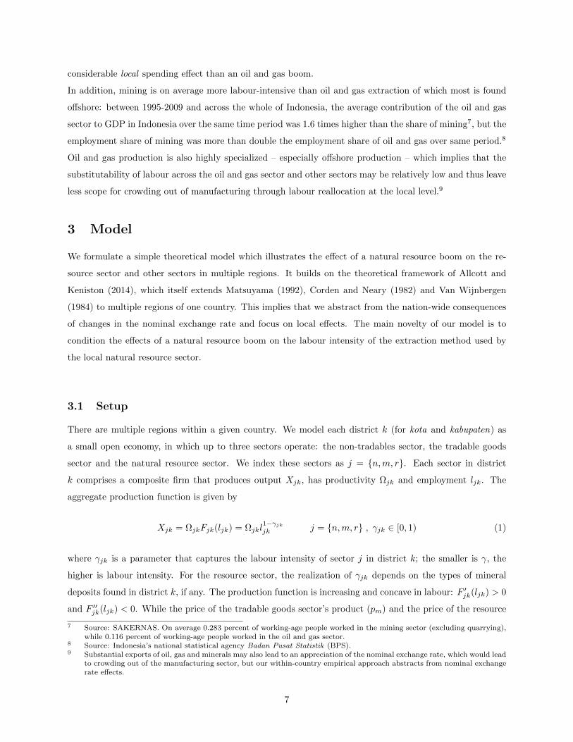
considerable local spending effect than an oil and gas boom.

In addition, mining is on average more labour-intensive than oil and gas extraction of which most is found

offshore: between 1995-2009 and across the whole of Indonesia, the average contribution of the oil and gas

sector to GDP in Indonesia over the same time period was 1.6 times higher than the share of mining7, but the

employment share of mining was more than double the employment share of oil and gas over same period.8

Oil and gas production is also highly specialized – especially offshore production – which implies that the

substitutability of labour across the oil and gas sector and other sectors may be relatively low and thus leave

less scope for crowding out of manufacturing through labour reallocation at the local level.9

3 Model

We formulate a simple theoretical model which illustrates the effect of a natural resource boom on the re-

source sector and other sectors in multiple regions. It builds on the theoretical framework of Allcott and

Keniston (2014), which itself extends Matsuyama (1992), Corden and Neary (1982) and Van Wijnbergen

(1984) to multiple regions of one country. This implies that we abstract from the nation-wide consequences

of changes in the nominal exchange rate and focus on local effects. The main novelty of our model is to

condition the effects of a natural resource boom on the labour intensity of the extraction method used by

the local natural resource sector.

3.1 Setup

There are multiple regions within a given country. We model each district k (for kota and kabupaten) as

a small open economy, in which up to three sectors operate: the non-tradables sector, the tradable goods

sector and the natural resource sector. We index these sectors as j = n,m, r. Each sector in district

k comprises a composite firm that produces output Xjk, has productivity Ωjk and employment ljk. The

aggregate production function is given by

Xjk = ΩjkFjk(ljk) = Ωjkl1−γjkjk j = n,m, r , γjk ∈ [0, 1) (1)

where γjk is a parameter that captures the labour intensity of sector j in district k; the smaller is γ, the

higher is labour intensity. For the resource sector, the realization of γjk depends on the types of mineral

deposits found in district k, if any. The production function is increasing and concave in labour: F ′jk(ljk) > 0

and F ′′jk(ljk) < 0. While the price of the tradable goods sector’s product (pm) and the price of the resource

7 Source: SAKERNAS. On average 0.283 percent of working-age people worked in the mining sector (excluding quarrying),while 0.116 percent of working-age people worked in the oil and gas sector.

8 Source: Indonesia’s national statistical agency Badan Pusat Statistik (BPS).9 Substantial exports of oil, gas and minerals may also lead to an appreciation of the nominal exchange rate, which would lead

to crowding out of the manufacturing sector, but our within-country empirical approach abstracts from nominal exchangerate effects.

7

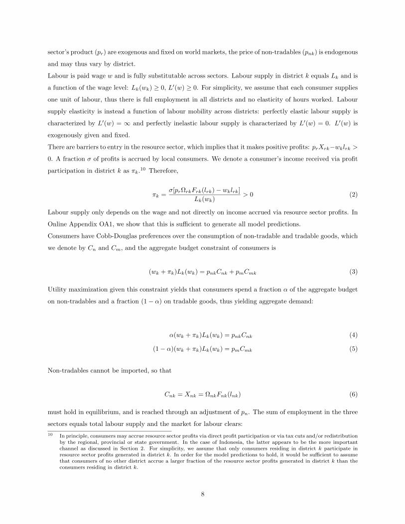
sector’s product (pr) are exogenous and fixed on world markets, the price of non-tradables (pnk) is endogenous

and may thus vary by district.

Labour is paid wage w and is fully substitutable across sectors. Labour supply in district k equals Lk and is

a function of the wage level: Lk(wk) ≥ 0, L′(w) ≥ 0. For simplicity, we assume that each consumer supplies

one unit of labour, thus there is full employment in all districts and no elasticity of hours worked. Labour

supply elasticity is instead a function of labour mobility across districts: perfectly elastic labour supply is

characterized by L′(w) = ∞ and perfectly inelastic labour supply is characterized by L′(w) = 0. L′(w) is

exogenously given and fixed.

There are barriers to entry in the resource sector, which implies that it makes positive profits: prXrk−wklrk >

0. A fraction σ of profits is accrued by local consumers. We denote a consumer’s income received via profit

participation in district k as πk.10 Therefore,

πk =σ[prΩrkFrk(lrk)− wklrk]

Lk(wk)> 0 (2)

Labour supply only depends on the wage and not directly on income accrued via resource sector profits. In

Online Appendix OA1, we show that this is sufficient to generate all model predictions.

Consumers have Cobb-Douglas preferences over the consumption of non-tradable and tradable goods, which

we denote by Cn and Cm, and the aggregate budget constraint of consumers is

(wk + πk)Lk(wk) = pnkCnk + pmCmk (3)

Utility maximization given this constraint yields that consumers spend a fraction α of the aggregate budget

on non-tradables and a fraction (1− α) on tradable goods, thus yielding aggregate demand:

α(wk + πk)Lk(wk) = pnkCnk (4)

(1− α)(wk + πk)Lk(wk) = pmCmk (5)

Non-tradables cannot be imported, so that

Cnk = Xnk = ΩnkFnk(lnk) (6)

must hold in equilibrium, and is reached through an adjustment of pn. The sum of employment in the three

sectors equals total labour supply and the market for labour clears:

10 In principle, consumers may accrue resource sector profits via direct profit participation or via tax cuts and/or redistributionby the regional, provincial or state government. In the case of Indonesia, the latter appears to be the more importantchannel as discussed in Section 2. For simplicity, we assume that only consumers residing in district k participate inresource sector profits generated in district k. In order for the model predictions to hold, it would be sufficient to assumethat consumers of no other district accrue a larger fraction of the resource sector profits generated in district k than theconsumers residing in district k.

8

lnk + lmk + lrk = Lk(wk) (7)

Since each composite firm maximizes profits, in equilibrium the marginal product of labour of all sectors

equals the wage:

wk = pnkΩnkF′nk(lnk) = pmΩmkF

′mk(lmk) = prΩrkF

′rk(lrk) (8)

= pnkΩnk

[1− γnklγnknk

]= pmΩmk

[1− γmklγmkmk

]= prΩrk

[1− γrklγrkrk

](9)

3.2 The effects of a natural resource boom

We trace the effect of a natural resource boom through the model, which we define as an increase in the

world price of natural resources, pr. Alternatively, equivalent predictions follow from defining a boom as an

increase in the resource sector’s productivity, Ωrk. This generates four predictions. We provide intuition

below and delegate formal proofs to the Online Appendix.11 To keep the notation parsimonious, we drop

the k-subscript in the following.

Prediction 1: A natural resource boom increases (i) the wage and (ii), if labour supply is not perfectly in-

elastic, also population. Further, (iii) a natural resource boom increases resource sector employment.

The increase in the world price for natural resources increases the marginal product of labour in the resource

sector, which responds by hiring more workers. Attracting these workers requires an increase in wages from

other sectors (which in the Corden and Neary (1982) terminology is called the“resource movement effect”),

or from other districts as long as L′(w) > 0. Such migration dampens the increase in wages, and the more

so the higher is labour mobility across districts.

Prediction 2: A natural resource boom increases the production and price of non-tradables.

The non-tradable sector faces higher demand from wealthier local consumers after a rise in pr. Since it

is able to pass on the costs of increased wages to consumers via raising prices, it is profit-maximizing for

the sector to respond by an increase in production. As long as labour supply is not fully inelastic, the rise

in demand and production for non-tradables is caused by two factors: a) consumers participate in natural

resource sector profits (i.e. σ > 0 and thus π > 0), which is the “spending effect” in Corden and Neary

11 Note that in order to prove Predictions 1-3, it is sufficient to assume that the general production function is increasingand concave in labour, i.e. F ′jk(ljk) > 0 and F ′′jk(ljk) < 0.

9

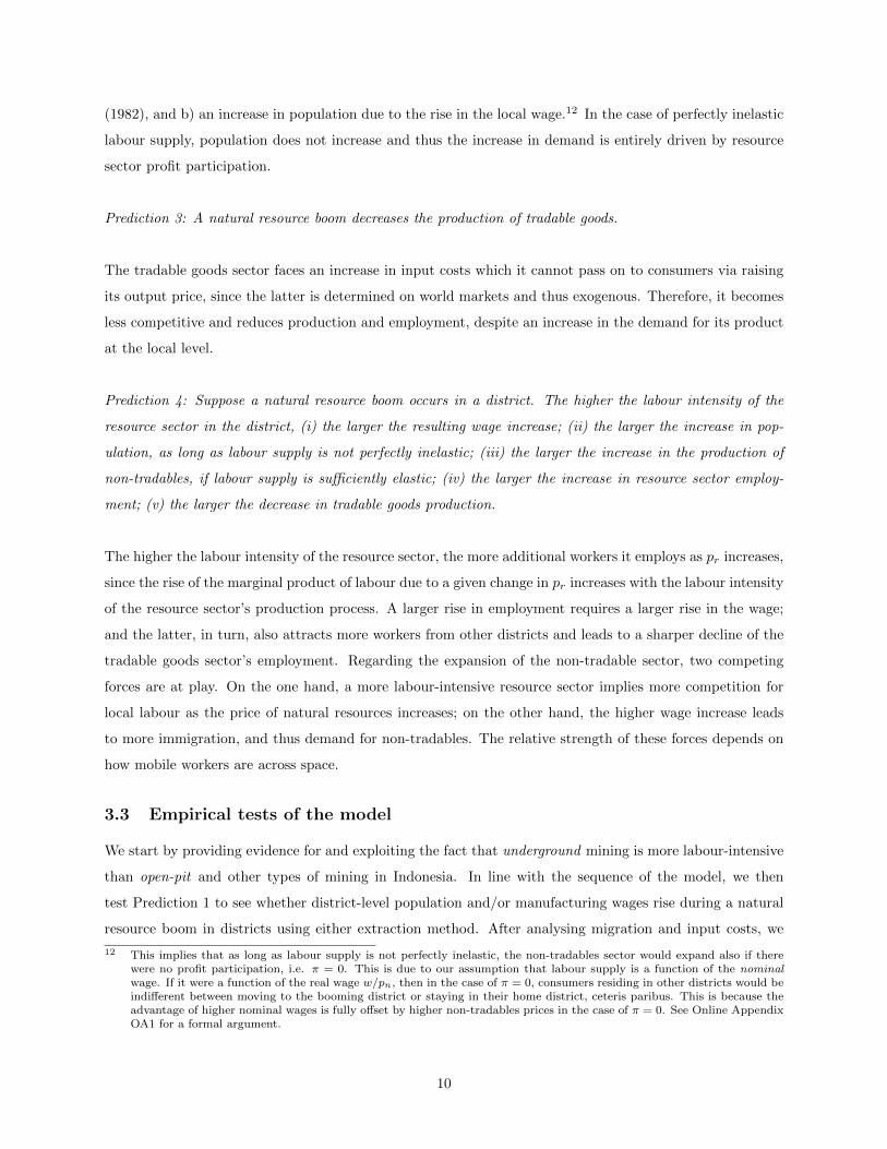
(1982), and b) an increase in population due to the rise in the local wage.12 In the case of perfectly inelastic

labour supply, population does not increase and thus the increase in demand is entirely driven by resource

sector profit participation.

Prediction 3: A natural resource boom decreases the production of tradable goods.

The tradable goods sector faces an increase in input costs which it cannot pass on to consumers via raising

its output price, since the latter is determined on world markets and thus exogenous. Therefore, it becomes

less competitive and reduces production and employment, despite an increase in the demand for its product

at the local level.

Prediction 4: Suppose a natural resource boom occurs in a district. The higher the labour intensity of the

resource sector in the district, (i) the larger the resulting wage increase; (ii) the larger the increase in pop-

ulation, as long as labour supply is not perfectly inelastic; (iii) the larger the increase in the production of

non-tradables, if labour supply is sufficiently elastic; (iv) the larger the increase in resource sector employ-

ment; (v) the larger the decrease in tradable goods production.

The higher the labour intensity of the resource sector, the more additional workers it employs as pr increases,

since the rise of the marginal product of labour due to a given change in pr increases with the labour intensity

of the resource sector’s production process. A larger rise in employment requires a larger rise in the wage;

and the latter, in turn, also attracts more workers from other districts and leads to a sharper decline of the

tradable goods sector’s employment. Regarding the expansion of the non-tradable sector, two competing

forces are at play. On the one hand, a more labour-intensive resource sector implies more competition for

local labour as the price of natural resources increases; on the other hand, the higher wage increase leads

to more immigration, and thus demand for non-tradables. The relative strength of these forces depends on

how mobile workers are across space.

3.3 Empirical tests of the model

We start by providing evidence for and exploiting the fact that underground mining is more labour-intensive

than open-pit and other types of mining in Indonesia. In line with the sequence of the model, we then

test Prediction 1 to see whether district-level population and/or manufacturing wages rise during a natural

resource boom in districts using either extraction method. After analysing migration and input costs, we

12 This implies that as long as labour supply is not perfectly inelastic, the non-tradables sector would expand also if therewere no profit participation, i.e. π = 0. This is due to our assumption that labour supply is a function of the nominalwage. If it were a function of the real wage w/pn, then in the case of π = 0, consumers residing in other districts would beindifferent between moving to the booming district or staying in their home district, ceteris paribus. This is because theadvantage of higher nominal wages is fully offset by higher non-tradables prices in the case of π = 0. See Online AppendixOA1 for a formal argument.

10

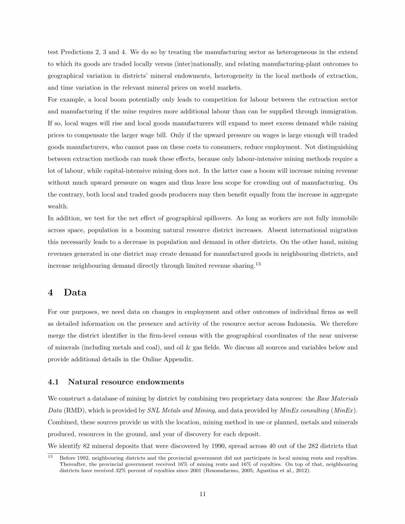
test Predictions 2, 3 and 4. We do so by treating the manufacturing sector as heterogeneous in the extend

to which its goods are traded locally versus (inter)nationally, and relating manufacturing-plant outcomes to

geographical variation in districts’ mineral endowments, heterogeneity in the local methods of extraction,

and time variation in the relevant mineral prices on world markets.

For example, a local boom potentially only leads to competition for labour between the extraction sector

and manufacturing if the mine requires more additional labour than can be supplied through immigration.

If so, local wages will rise and local goods manufacturers will expand to meet excess demand while raising

prices to compensate the larger wage bill. Only if the upward pressure on wages is large enough will traded

goods manufacturers, who cannot pass on these costs to consumers, reduce employment. Not distinguishing

between extraction methods can mask these effects, because only labour-intensive mining methods require a

lot of labour, while capital-intensive mining does not. In the latter case a boom will increase mining revenue

without much upward pressure on wages and thus leave less scope for crowding out of manufacturing. On

the contrary, both local and traded goods producers may then benefit equally from the increase in aggregate

wealth.

In addition, we test for the net effect of geographical spillovers. As long as workers are not fully immobile

across space, population in a booming natural resource district increases. Absent international migration

this necessarily leads to a decrease in population and demand in other districts. On the other hand, mining

revenues generated in one district may create demand for manufactured goods in neighbouring districts, and

increase neighbouring demand directly through limited revenue sharing.13

4 Data

For our purposes, we need data on changes in employment and other outcomes of individual firms as well

as detailed information on the presence and activity of the resource sector across Indonesia. We therefore

merge the district identifier in the firm-level census with the geographical coordinates of the near universe

of minerals (including metals and coal), and oil & gas fields. We discuss all sources and variables below and

provide additional details in the Online Appendix.

4.1 Natural resource endowments

We construct a database of mining by district by combining two proprietary data sources: the Raw Materials

Data (RMD), which is provided by SNL Metals and Mining, and data provided by MinEx consulting (MinEx ).

Combined, these sources provide us with the location, mining method in use or planned, metals and minerals

produced, resources in the ground, and year of discovery for each deposit.

We identify 82 mineral deposits that were discovered by 1990, spread across 40 out of the 282 districts that

13 Before 1992, neighbouring districts and the provincial government did not participate in local mining rents and royalties.Thereafter, the provincial government received 16% of mining rents and 16% of royalties. On top of that, neighbouringdistricts have received 32% percent of royalties since 2001 (Resosudarmo, 2005; Agustina et al., 2012).

11

existed in 1990. The year 1990 is chosen to fix endowments at the start of the period for which we observe

manufacturing outcomes.14 The deposits represent a wide variety of minerals, which each have their own

world price as shown in Figure 2.15 The most common extraction method is open-pit mining, which was

listed for 77 deposits in 36 districts, followed by 11 deposits in nine districts listed as operated or planned to

be operated by underground mining, while only three deposits in three districts use placer mining techniques

for deposits found in (former) river beds.16

To aggregate deposits with different minerals by district we first compute for each deposit the remaining

discovered mineral ore resources as of 1990, measured in megatons.17 We then sum across deposits by district

and divide by the surface area of the 1990 district. We use ore rather than the mineral or metal content

because the primary response to a price shock is arguably an adjustment of ore production: the more ore

resources a developed deposit has, the larger its operations and the potential effects on the labour market.

We thus define the district-level endowment measure rk as follows:

rk =

∑dRdk

Areak(10)

where Rdk stands for the ore resources of deposit d in district k in 1990. Finally, we scale rk by its average

across all positive realizations of rk and label this rk. Estimated coefficients can then be interpreted as the

effect of increasing mineral endowment by the average endowment of mining districts.

For oil and gas endowments we rely on a novel source, the Indonesia Oil and Gas Atlas by Courteney et

al. (1991), of which we digitize six volumes between 1988 and 1991. The six volumes list all oil and gas

fields in Indonesia that had been discovered at the time of publication, as well as their precise location and

“current daily production”, which equals the most recent available production figure. The benefit is that we

can include all fields without relying on an arbitrary size-cut off such as in the commonly used data base for

giant discoveries (Horn, 2003). Unfortunately, field-specific oil and gas remaining resources in the ground

are not reported. Therefore, we compute our proxy for oil and gas endowment as the sum of reported daily

production of barrels of oil equivalent (BOE) over all fields within a district (using the closest year available

to 1990 within the 1988-1991 period), divided by district size.18 We scale this proxy in the same way as we

scaled rk, and denote it ˜boek. 37 districts in 14 different provinces were producing oil and/or gas around

1990. Nine of these districts also contained minerals in 1990.

We relate these measures of endowment to world prices using a variety of sources for all the minerals and

14 Because districts in Indonesia proliferate over time we aggregate to the 1990 district borders. For the period 1990-1993we rely on Bazzi and Gudgeon (2018) and for other years on Indonesia’s national statistical agency Badan Pusat Statistik(BPS).

15 22 deposits hosted coal (which contained 72.63 percent of total resources), 20 gold (7.31%), 12 tin (2.39%), nine copper(9.44%), eight silver (5.3%), seven nickel (1.42%), six bauxite (0.75%), four iron ore (0.68%), two manganese (0.0006%),one cobalt (0.05%), one diamonds (0.01%), one uranium (0.01%) and one zirconium (0.0002%).

16 The numbers add to more than 82 because some mines use a combination of methods.17 If a deposit was mined before 1990, we deduct the mine’s pre-1990 ore production from the initial resources. Resources

are defined as “the concentration or occurrence of material of intrinsic economic interest in or on the Earth’s crust in suchform and quantity that there are reasonable prospects for eventual economic extraction” (Raw Materials Data Handbook,p.57)

18 We convert cubic feet of natural gas to barrels of oil equivalent by using a standard conversion factor of 6,000.

12

metals. We discuss the construction of the mineral price index in detail in the next section, which interacted

with initial endowments constitutes our measure of a local natural resource shock.

Table 1 provides descriptive statistics on natural resource endowments by province and shows the geograph-

ical dispersion of endowments, which includes the populous islands of Java and Sumatra.

Other district-level variables include population from the population census rounds 1990, 2000 and 2010 and

the inter-census population surveys (SUPAS) of 1995 and 2005 as reported by the University of Minnesota’s

Minnesota Population Center (MPC), and the number of mining workers, which we approximate using the

SAKERNAS household survey using the district-representative years 2007 to 2015.

4.2 Firm data

To measure firm activity we use the annual census of manufacturing plants (Survei Industri (SI)), which

contains repeated observations on 59,031 manufacturing plants between 1990 and 2009 that employ at least

20 employees in a particular year. The data is collected and compiled by the BPS. The dataset contains

detailed information on performance indicators, including employment, investment, material inputs, revenue,

exports, price deflators, products sold, and the district in which the plant is located. In addition, it contains

a 4-digit ISIC sector classification. The census covers the manufacturing sector and thus excludes mining

operations. Table 2 presents the descriptive statistics.

Our main outcome variable is employment as reported in the census.19 We do not observe hours worked so

we construct plant-year level earnings per worker by dividing the total wage bill by the number of employees.

Revenue as reported in the census is the value of goods produced. The number of products sold and the

average unit price (equal to revenues divided by the total number of products sold) are only available from

1998 onwards, which restricts the sample size to 1998-2009 for these outcomes. Finally, we obtain total

factor productivity from Javorcik and Poelhekke (2017).20 We only observe continuing plants with 20 or

more employees and thus cannot identify entry and exit. If mining booms have larger effects on smaller

plants or result in plant exits, then our estimates provide a lower bound on the actual effect.

We use the detailed sector classification and export data to construct indicators for whether a plant mainly

sells to local markets or whether it sells to non-local and foreign markets. This is important because local

goods producers may be able to pass on higher labour costs to an expanded local market, while traded

goods producers that are price takers would lose market share. While the manufacturing sector is usually

19 Total employment at the plant level includes paid and unpaid workers. The reported number of total workers per plantcorresponds to the respondent’s assessment of the plant’s average employment in the survey year.

20 TFP calulation is based on the method by De Loecker Warzynski (2012) and Ackerberg et al. (2006). First, a separatetranslog production function for each two-digit ISIC sector is estimated, relating the log value added to (the log of)capital, labour, and materials (including squared terms and all interactions) and year and four-digit-ISIC-industry fixedeffects. Input coefficients are allowed to vary by exporter and foreign ownership status. Demand for materials proxiesfor unobservable productivity shocks. This yields expected industry-level output, which then results in plant-year leveldeviations from expected output. In the second step, these are regressed using GMM on its lag, capital and labour inputwhere current labour is instrumented with lagged labour as suggested by Ackerberg et al. (2006). Finally, the innovations ofthis regression capture TFP. Value added equals output net of inputs of material and energy. Capital is proxied with fixedassets, labour with the number of employees. All variables are expressed in Indonesian rupiahs, deflated using five-digitindustry producer price indices.

13

regarded as altogether tradable, some manufacturing plants produce goods that are more tradable than

others. Further, a plant’s product may be highly tradable in its nature, but may de facto not be traded

beyond the local economy. We first divide plants into a group that never exports (non-exporters) and a

group that exports a positive fraction of its output in at least one year over our sample period (exporters).21

However, non-exporters may nevertheless sell goods in other districts and provinces within Indonesia and

be price-takers in those destinations.22 We therefore also split plants into local goods producers and traded

goods producers. Traded goods producers are plants that exported in at least one year in our sample period

(and thus contains all exporters), and/or, are plants that have a low (below four-digit industry median)

distance elasticity to trade. The latter equals the percentage change in trade volume as distance increases

by one percent as calculated by Holmes and Stevens (2014) using industries’ average shipment distance as

reported in the US Commodity Flow Survey. Our sample includes 123 four-digit manufacturing industries,

which results in “Ready-mixed concrete production” as the most locally-traded manufacturing sector, and

“Manufacture of engines and turbines, except aircraft, vehicle and cycle engines” as the most traded sector.23

Because similar data is not available for Indonesia we use US elasticities. This implicitly implies that we

assume that the ranking of industries with respect to distance elasticity across the two countries is the

same.24 Local goods producers are thus all other plants, which have an above median distance elasticity.

Finally, some of the plants in our data may be upstream to the mining sector. Upstream plants are potential

suppliers to mines and defined as those plants that operate in four-digit industries that sell an above median

share of output to the mining sector. To compute this, we rely on input-output tables for the United States,

as discussed in the Online Appendix.25

21 Defining export status at the plant level might be problematic due to selection effects. For example, suppose that districtswith positive 1990 mineral resources decide to implement exporter-friendly policies during the sample period, and thatthese policies only bite during mining booms. Also suppose that these policies cause new manufacturing plants (call themthe group of plants A) to settle in such districts, and that in mining districts, there are other plants in the same industriesas the exporting plants which do not export (group of plants B), but whose prices are not determined locally. If we thencompare the performance of exporters vs. non-exporters, we may find no effect. A solution to this potential problem wouldbe to define export status at the industry level, as this would put the group of plants A and B, respectively, in the samecategory. However, this is not possible since only in one of the 123 four-digit industries in our sample, no plant exporteda positive fraction of output over the sample period. That said, we consider the likelihood of such selection issues as verylow.

22 A large fraction of tradable goods producers may not export their output due to insufficient competitiveness or bureaucraticreasons (see e.g. McLeod, 2006)

23 Since the Holmes & Stevens measure is industry-specific, and some plants in our sample change industry over time, itis possible that a plant changes status over time. As we discuss in section 6.6.2, our results are robust to droppingindustry-switchers.

24 If this nonetheless introduces measurement error it will be harder to reject the null hypothesis that the effect of miningbooms differs across producers of traded versus local goods producers.

25 These tables are as of 2007 and provided by the Bureau of Economic Analysis (BEA). We prefer the US input-outputtables since they distinguish more sectors than any Indonesian input-output table does, and thus allows a finer evaluationof an industry’s linkage to the mining sector. While for many sectors using the input-output table of another country maygive a poor image of the industry’s linkage to other industries, this is not the case for the mining sector, as formal miningis done in a very standard way across the globe.

14

5 Empirical Strategy

Our main hypothesis is that an outcome variable of plant i in industry j in district k is affected by the

intensity of mining activity in district k. We thus need exogenous variation in mining activity over time

at the district level. Further, we expect the magnitude of the effect of mining booms to depend on the

labour intensity of the local mining methods used. We establish the relevance of this margin in preliminary

regressions in Section 6.1.

As suggested by the model, a natural resource boom is an increase in the world price of natural resources.

Since districts may host multiple deposits each containing multiple minerals we construct a price index

that captures the price level of resources found in existing deposits in each district, using as weights the

district-specific share of mineral m in total initial 1990 resources. More precisely we define:

ln(MinPricekt) = ln

[∑m [Pmt ∗

∑dRmdk]∑

dRdk

]if∑d

Rdk > 0, 0 otherwise

where Pmt equals the world price of mineral m in year t indexed to base year 1990 and Rmdk equals the 1990

ore resources of mineral m in deposit d in district k. Figure 2 plots the development of Pmt for all minerals

in our sample and shows periods with large price swings. For example, the steep increase in the price of

iron ore as observed in 2005 will have no effect in districts without iron ore deposits (absent spillovers),

and only a substantial effect in districts where iron ore makes up a large share of ore endowments. Fixing

weights to the base year 1990 and using only deposits that were discovered by 1990 ensures exogeneity with

respect to plant-level outcomes in subsequent years, conditional on plant (and district) fixed effects, which

we absorb by first differencing. Finally, the mining method is closely related to the geological shape in which

the deposit occurs, which is exogenous (Hartman and Mutmansky, 2002).

Given this price level definition, we can write down our main estimating equation where we follow the

approach of Allcott and Keniston (2018) for oil and gas development in the US, but adjust for the presence

of multiple minerals and for variation in extraction techniques:

∆lnYijkt = β1∆[ln(MinPricekt) ∗ rk] + β2∆[ln(MinPricekt) ∗ rk ∗ Undergroundk]

+β3∆[ln(OilPricet) ∗ ˜boek] + β4rk + β5 ˜boek + β6Undergroundk + β7[rk ∗ Undergroundk]

+αt ∗ ωj + εijkt (11)

where Yijkt equals outcome Y of plant i in industry j in district k in year t, and αt ∗ ωj are four-digit

industry-year effects. Undergroundk is a dummy that equals one if at least one deposit in district k that

had been discovered by 1990 was operated or planned to be operated by underground mining. αt are year

fixed effects and ωj are industry fixed effects. We estimate equation (11) for all plant-specific outcome

15

variables and always cluster standard errors at the district-level.26

By first-differencing the outcome variable, we control for plant-specific and district-specific fixed effects. By

dropping plants before or after they move from one district to another, we ensure that district fixed effects

are nested within the plant fixed effects.27 We choose a first-difference rather than fixed-effects estimator

for two reasons: First, because the errors in equation (11) in levels are highly serially correlated and the

first-differences estimator is thus more efficient; and second, because this allows us to control for differential

trends in the outcome variables across districts that differ in terms of natural resource endowment and locally

applied mining techniques. To account for these differential trends, we include in the equation the scaled

mineral resource measure rk and oil equivalent production measure ˜boek. Similarly, we include a mining

method dummy Undergroundk and its interaction with rk separately in order to control for differential

trends in manufacturing outcomes in districts with labour-intensive mineral extraction methods. This also

captures differences in labour market trends. β1 is an unbiased estimate of the relative effect of a mining

boom on a manufacturing plant’s outcome Y as long as mining booms are uncorrelated with unobserved

economic trends, conditional on the control variables in equation (11). β1 measures a relative rather than

absolute effect: the counterfactual is the change in outcome Y in the same year of a plant in the same

industry, in a district that faces a smaller or no mining boom. For example, a doubling of local mineral

prices has a 100*β1 percent relative effect on the outcome variable in a district with average 1990 mineral

ore resources (i.e. rk = 1), compared to a plant in a district with no mineral resources. At the same time, it

can be interpreted as the differential effect of a given price increase in a district with endowments equal to

rk = 2 compared to a district with average endowments rk = 1.

In the absence of geographic spillovers, β1 will equal the absolute effect. Spillovers may occur via migration

from other districts into the booming district, the revenue sharing scheme through which near districts bene-

fit from mining booms, and an increase in demand for goods produced in near districts. In order to gauge the

effect of spillovers and thereby also understand their effect on β1, we develop two additional specifications.

In the first, we test the effect of a mining boom in neighbouring districts on the home district’s outcomes. In

the second, we test the effect of a mining boom in other districts in the same province on the home district’s

outcomes. In Section 6.6.1 we show that these effects are small and insignificant, suggesting that β1 comes

close to a measure of the absolute rather than relative effect of a mining boom.

26 We adjust the degrees of freedom for singleton industry-year groups, i.e. plants for which no other plant is in the sameindustry in a given year, following (Correia, 2015).

27 For each such plant, we keep the longest period in which the plant stays in one district. We cannot be sure if these eventsare real or due to measurement error. In a robustness test we drop them entirely.

16

6 Results

6.1 Does labour intensity differ by extraction method?

A rise in local input costs during a natural resource boom is a necessary condition for the manufacturing

sector to be negatively affected by the boom and any Dutch disease effects to occur. Our theoretical

predictions highlight that the larger the labour intensity of the natural resource sector, the more wages rise

during booms.

Our data distinguishes between underground, open-pit, and placer mining. According to Hartman and

Mutmansky (2002) underground mining methods are most labour intensive because it is harder to operate

and automate heavy machinery in underground tunnels.28 Conversely, all non-underground mining methods

(open-pit, open-cast, placer, auger mining and quarrying) are classified as non-labour-intensive. This suggests

that on average, and considering relatively low wage levels, that underground mining in Indonesia is more

labour-intensive than other types of mining and that mines that use a combination of underground and

open-pit methods are also more labour intensive than pure open-pit mines. In theory, labour can be the

predominant input in open-pit mining as well, if wages are sufficiently low. District fixed effects absorb

labour market conditions that would induce open-pit mines to use mostly labour instead of capital, because

even if labour market conditions change over time, it is unlikely that open-pit mines can switch from year to

year between capital-intensive machinery and labour-intensive alternatives without incurring prohibitively

high switching costs. Oil and gas extraction, some of which occurs offshore, is probably least labour intensive.

We test this more formally using the SAKERNAS household survey, providing us with an estimate of the

number of mining and oil & gas workers in each district, between 2007 and 2015.29

We first regress the dependent variable on the district’s total 1990 mineral resources and its oil and gas

production around 1990 (Table 3, column 1). Both variables are scaled by their respective average across

districts with positive realizations, but not scaled by district size. We also include year fixed effects and

cluster standard errors at the district level. The results suggest that a district with average 1990 mineral

resources employs 39 percent more mining and oil & gas workers than a district with no 1990 mineral

resources. In contrast, a district with average 1990 oil production employs only seven percent more mining

and oil & gas workers than a district with no 1990 oil and gas production. This cannot be explained by a

difference in overall relevance of mining compared to oil and gas extraction: An inspection of Indonesia’s

national accounts reveals that the average mining district only contributed 5% more to overall GDP than

the average oil and gas district over 2007-2014. This corroborates our prior that oil and gas extraction is

least labour-intensive.

28 Our data is not more specific, but in theory these can be further broken down into cut-and-fill stoping, stull stoping,square-set stoping, room-and-pillar mining, stope-and-pillar mining, shrinkage stoping and sublevel stoping, where thefirst three methods belong to the class of “supported” underground methods (to prevent collapse) and the latter four tothe class of “unsupported” mining methods. With the exception of stope-and-pillar mining and sublevel stoping, all ofthese methods are classified as relatively labour-intensive.

29 Manning (2006) suggests that the survey is suitable for estimating long-term trends of employment, but that it is notsuitable to study year-to-year changes.

17

In column 2 of Table 3, we include underground mining, a dummy equal to one if natural resource extraction

was at least partly done using underground methods. The results suggest that conditional on the district’s

mineral endowment, mining employment in underground mining districts is 107% larger than in other dis-

tricts.30 Column 3 shows that this result is driven by the districts in which all deposits use only underground

mining, rather than the districts in which both underground and open-pit mining occurs.31 In column 4 we

add province fixed effects to account for differential regional wages. The coefficient on oil and gas production

is now close to zero and not significant, while the coefficient on underground and open-pit mining is now

positive and (marginally) statistically significant, but the ranking in terms of labour-intensity is preserved.

These results clearly support the claim that underground mining is more labour-intensive than other types

of mining in Indonesia.

Our second test uses population data. If indeed underground mining is more labour-intensive, we would also

expect a stronger population response to a booming mining sector that employs more labour, relative to other

mining districts. Second, as highlighted by the model, low overall labour mobility is a necessary condition

for wages to rise during a boom. Since population data is only collected every five years in Indonesia, we

adapt equation (11) to examine the effect of mining and oil & gas booms on immigration. The dependent

variable is the change in log population during four periods, covering 1990-1995, 1995-2000, 2000-2005, and

2005-2010. Table 4 presents the regression results, where we relate annual mineral price changes in three

different ways to five-yearly population changes. The first measure takes the simple average of all five annual

price changes (columns 1 and 2). In our second measure, we assume that price shocks towards the end of

the five-year period have a stronger effect on the five-year change in population, and specifically determine

the weights as ω = 0.3, 0.25, 0.2, 0.15, 0.1 (column 3). In our third measure, we simply compute the price

shock as the difference between the current district-specific minerals price and its five-year lag (column 4).

In each specification, we interact the price change measure with our scaled mineral resource measure rk –

which we label Mineral Resources 1990 in all tables – and with the interaction of rk and the dummy variable

Underground Mining. In column 1, we estimate the average effect, while in columns 2-4 we distinguish

between the two mining methods. Standard errors are clustered at the district, in order to account for

possible serial correlation in the error term and heteroskedasticity.

The results suggest that an increase in the price of local minerals does spur immigration into mining districts

(see column 1), dampening a response of wages. However, column 2 shows that labour mobility during mining

booms clearly depend on local extraction methods. If mining is more capital-intensive, booms do not affect

population. We also find that oil and gas booms do not spur significant immigration. This is consistent with

oil and gas extraction being very capital-intensive and the fact that most revenue accrues to the central as

opposed to local governments as explained in Section 2. Labour supply in Indonesia appears less responsive

30 Online Appendix Table OA1 shows that the results of Table 3 on mining are very robust to restricting the dependentvariable to mining employment only and excluding oil and gas production from the set of controls.

31 We do not know the relative mix of methods used in deposits where both underground and open-pit is used. The threedistricts where all deposits use only underground mining are in the districts of Bogor and Lebak on densely populatedJava, and Sintang on sparsely populated Kalimantan (Borneo). Dropping one of the 9 districts at a time does not affectthe main results, see Online Appendix Table OA2.

18

to natural resource booms than in the United States, since Allcott and Keniston (2018) find that population

significantly increases in oil and gas counties as the oil price doubles (by a mere 0.3 percent, however).

When local mining is labour-intensive, labour supply in Indonesian mining districts does increase during

boom times, although the effect is not large. Column 2 indicates that if the district-specific mineral prices

double each year over a period of five years, then district population significantly increases by 6.1 percent, in

the district with average mineral resources and where underground mining takes place. If the price of local

minerals doubles compared to five years ago, the population of the average mining district significantly rises

by 1.2 percent, if underground mining takes place (column 4). Because the size of the median price shock is

12%, the economic magnitude of the coefficients appears relatively small.32 Overall, our results suggest that

while labour is not immobile across space as a response to minerals price shocks, labour mobility is relatively

low. This should lead to upward wage pressure and potential Dutch disease mechanisms, which we examine

next.

6.2 Manufacturing Earnings per Worker

We estimate equation (11), using as dependent variable the log change in average earnings per worker and

present the results in Table 5 for different groups of manufacturing plants. For ease of interpretation, we

list the marginal effect of the price effect for districts that use underground, labour-intensive mining at the

bottom. Column 1 shows that there is no average effect of mining nor of oil and gas booms on earnings

per worker. However, column 2 shows that in districts with average mineral resources that use underground

mining methods, a doubling of local mineral prices leads to a significant increase of earnings per worker by

5.9 percent. This novel result is consistent with our theoretical framework: if mining is labour-intensive,

a mine needs to attract more additional workers to expand production, which requires a larger increase in

wages. It also suggests that immigration into these districts is driven by higher wages, but is not elastic

enough to keep wages flat. Relatively capital-intensive extraction methods such as open-pit mining and oil &

gas extraction yield no wage response, perhaps because the higher degree of capital intensity requires workers

with more specific skills that are imperfect substitutes for manufacturing workers, or because the elasticity

of oil production to oil prices is lower. Anderson et al. (2018) indeed find that skill and capital-intensive

drilling is more responsive to oil prices than oil production itself, which may be why Cust et al. (2017) find

a positive response of wages after an oil price increase in districts that explored for oil and had success. We

find that the intensive margin of extraction is more relevant for mining than for oil.

Columns 3-5 explore the differential effect of a mining boom on local versus traded goods producers. We find

that the increase in earnings per worker during labour-intensive mining booms is driven by manufacturing

plants producing local goods, who are more likely to be able to pass on wage costs to local consumers.

Exporters and traded goods producers in general do not raise wages during a boom, but there is some

limited evidence that exporting plants in labour-intensive mining districts may be worse off than exporters

32 Calculated as the median of absolute mineral-specific price shocks, weighted by the frequency of occurrence of the mineral.

19

located in districts with capital-intensive mining methods. The coefficients are very robust to how we define

producers of local and traded manufacturing goods, as a comparison of the results in column 2 and 4, and 3

and 5, reveals. However, because at the same time unobserved hours worked may increase, it is not a given

that costs rise. We thus look at employment next.

6.3 Manufacturing employment

Table 6 presents the results for manufacturing employment. Column 1 shows that employment expands

to meet excess demand for goods in now richer districts, although the effect is small and only significant

with 90% confidence. However, conditioning on extraction methods in column 2 shows that manufacturing

plants only hire significantly more workers during capital-intensive mining booms, while employment is

unaffected by labour-intensive mining booms. Together with our results on earnings per worker, this suggests

that manufacturing plants benefit from a spending effect during both capital- and labour-intensive mining

booms (through resource revenue sharing with local governments), but that this benefit is offset by upward

pressure on their wage bill during labour-intensive booms.33 The beneficial (local) spending effect leads to

an expansion of non-exporters and local goods producers, which does not depend on extraction methods.

A sudden increase in the value of oil production does not lead to more employment at the local level,

because it accrues mostly to the central government. The negative albeit limited effects of factor reallocation

between local and traded goods producers are apparent in columns 4 and 6, but only in labour-intensive

mining districts. A boom then leads to a reduction in employment of 1% for exporters. Capital-intensive

booms also feature a positive spending effect, but do not increase wages, which thus also raises employment

for exporters and traded goods producers. In fact, and despite the theoretical result that traded goods

producers and exporters benefit less from the spending effect, in this case exporting plants appear to benefit

more than non-exporters. This could be due to increased demand for higher quality, which is offered by

firms that compete in (inter)national markets.34

The results are again very consistent across the two chosen ways of identifying producers of local versus

traded goods. For all remaining dependent variables, we therefore focus only on our preferred method,

which takes both the plant-specific export status as well as the industry-specific distance elasticity into

account.

6.4 Manufacturing revenue, products sold, and prices

Table 7 reports results on manufacturing revenues (Panel A), products sold (Panel B), and prices (Panel

C). For capital-intensive booms, for all plants on average and for local goods producers, the coefficients

are positive, but they are not significant. We do find large positive and significant effects during labour-

33 Prediction 2 of the model also relates the spending effect to an increase in population via an increase in wages. The weakresponse of earnings per worker during capital-intensive booms in Table 5 suggest this channel is less empirically relevant.

34 Note that we control for sector-year fixed effects, which absorb sector-specific global demand shocks that may correlatewith mineral booms.

20

intensive booms for local goods producers. They increase average product prices (rather than units sold) by

15.3 percent as local mineral prices double (Panels B and C). Local goods producers are thus able to pass on

the costs of higher wages and this directly translates into larger revenues (Panel A). Capital-intensive booms

in contrast are only loosely related to higher prices and more products sold. Traded goods producers do not

significantly change prices nor products sold during labour-intensive mining booms, but the combined effect

nevertheless translates into somewhat higher revenue (1.2 percent), despite the contraction in employment.

The oil price has again a much smaller or no effect with only a significant increase in revenues of 0.3 percent

reflecting a very limited local spending effect from oil.

We thus find strong evidence in favour of the model and a reallocation of employment from traded to

non-traded sectors, but only during labour-intensive mining booms. As in Corden and Neary (1982), this

reallocation on its own is efficient and in theory welfare improving. In fact, we find that the manufacturing

sector as a whole does not do worse in terms of employment in booming districts. To gauge potential longer

term effects we next estimate the effect on total factor productivity.

6.5 Total Factor Productivity

Columns 1-3 of Table 8 present the results on the effect of contemporaneous mining booms on (innovations

to) total factor productivity (TFP). While TFP is largely unchanged during capital-intensive booms, it sig-

nificantly increases for local plants during labour-intensive booms. This is probably to a large extent driven

by the significant and large increase in revenues. For traded goods producers, the small contraction in em-

ployment may result in negative ‘learning by doing’ effects as in Van Wijnbergen (1984) and Arrow (1962),

but the results displayed in column 3 suggest that traded goods producers experience a marginally significant

decrease in TFP during capital -intensive booms (when employment rises), while TFP is not significantly af-

fected during labour-intensive booms (when employment contracts), at least in the short run. In column 4,

we test whether such effects materialize with a lag. Specifically, we replace the dependent variable by the

change in TFP between t and t− 5. On the right-hand side, we replace the price shocks with respect to the

previous year by the average change in annual prices. Thus, the coefficient must be interpreted as the effect

of a doubling of minerals prices in each year over the five-year period. The coefficient is not significant: while

we do observe that traded sector employment is crowded out during a labour-intensive mining boom, this

has no effect on productivity. Although factor reallocation occurs, the evidence for a productivity-related

‘Dutch disease’ thus remains elusive.

21

6.6 Additional results and robustness checks

6.6.1 Regional spillovers and revenue sharing

So far we did not account for the possibility that regional spillovers affect the results. Testing for such

spillovers sheds light on whether we estimate an effect that is relative to other districts, or an absolute effect

of mining booms. In Table 9 we first repeat the baseline for comparison and in column 2 we control for

mining booms/busts in neighbouring districts with which it shares a border.35 We treat all neighbours as

one single district and compute its mineral resources per square mile as of 1990 and price shock realizations

analogously to the single-district computation. In column 3, we control for the average mining boom in other

districts of the same province, which may have an effect on plants in the home district via natural resource

revenue sharing (see Section 2). The coefficients on the spillover variables in column 2 and 3 are close to zero

and statistically insignificant, which suggests that spillovers of local mining booms to neighbouring districts

or districts in the same province are not empirically relevant on average. Combined with the evidence for

relatively low labour mobility, we conclude that the coefficients in our main specification come close to

representing absolute rather than relative effects.

In addition, we test whether increased revenue sharing with other districts since decentralization helps to

spread any benefits of mining booms beyond the mining district itself.36 In 1999 a new law on revenue

sharing of natural resource rents between the national government, provinces, and districts was signed.

Law 25/1999 stipulated that the producing district’s share in royalties decreased from 64 to 32%, and that

districts in the same province of the producing district would get 32% instead of 0%. We test whether

increased revenue sharing between resource-rich and resource-poor districts after 1999 has led to (i) stronger

spillovers of mining boom into neighbouring districts and other districts in the same province and to (ii)

weaker spending effects in the booming district itself. Rather than adding another interaction we restrict

the sample to the years 1999 and after, and rerun regressions (2) and (3). Columns 4 and 5 show that there

is again no evidence for spillovers, and weak evidence on slightly smaller spending effects.

Finally, allowing for arbitrary correlation of the errors across space by clustering on district and year does

not affect the main results (column 6). Because there are only 19 years and thus 19 clusters in the sample

we follow best practise and do not cluster by year throughout (Cameron and Miller, 2015).

6.6.2 Robustness checks

Endowments in 1980

While labour market trends may differ between districts of varying mining intensity, we control for these in

our main specification through including rk and its interaction with the underground mining dummy (see

35 Since a number of districts are islands, they do not have neighbours according to our definition. This implies that thesample size in the robustness check of column 2 is slightly smaller compared to our baseline specification.

36 Since we are interested in controlling for spillover effects due to revenue sharing and the latter occurs independentlyof the local mining methods, we do not feature an additional interaction with the underground mining dummy in thisspecification.

22

equation 11), and by fixing natural resource endowments in 1990 and thus before we observe plant-level

outcomes. Thereby we also control for any systematically different unobserved exploration trends that may

affect annual changes in manufacturing outcomes. Nevertheless, we further address this concern by timing

mineral resources per square mile in 1980 in columns 2 of Table 10. We still scale by the average realiza-

tion of mineral resources in the year 1990 such that the endowment is expressed in units of average 1990

endowment.Because 1980 endowments are smaller resulting in a mean of rk,1980 = 0.675, instead of 1 for

rk, we find larger coefficients but the overall pattern and marginal effect of labour-intensive booms is the same.

Industry switchers

Some plants switch industry and potentially also between the industry-level categories of local and traded

goods producers, which may be correlated with local natural resource booms, and lead to measurement error

and potentially bias the results if the industry-switch is endogenous. In column 3 we exclude all plants that

ever switch 4-digit ISIC industry. Despite losing almost a third of observations, the coefficients are robust

to this change.

Foreign and state owned plants

In column 4 of Table 10, we examine whether our results are homogeneous across plants of different ownership

structure. Government ownership may for example insulate plants from Dutch disease effects. We control

for lagged ownership by interacting the mining boom variable as well as its interaction with the underground

mining dummy with a plant-specific foreign ownership and a government ownership dummy, respectively.

The former equals one if the plant was partly or fully foreign-owned in t− 1, and the government ownership

dummy equals one if the plant was partly or fully owned by the local and/or central government in t−1. We

find that foreign-owned plants benefit much more from capital-intensive booms than domestic private and

government-owed plants. In particular, in the district with average mineral resources, foreign-owned plants

increase employment by 14.8 percent as minerals prices double, while domestic private plants significantly

increase employment by 2.5 percent and government-owned plants do not grow at all. The latter result

suggests that the central or local governments do not use mining windfalls to shield or promote the manufac-

turing plants they partly or fully own, and that those plants benefit less from a rise in local purchasing power

than is suggested by the results on privately-owned plants.37 During labour-intensive booms, government

owned plants are especially hit hard.

Upstream plants

Next, we check whether the results are driven by upstream plants that supply to the mining sector and

may locate in and directly benefit from districts with mining. Because the upstream dummy is defined

37 One potential explanation is that government-owned plants produce goods for the central government which are moretradable than the products of other plants. However, additional results that are available upon request show that alsogovernment-owned plants producing local goods do not significantly benefit from capital-intensive mining booms.

23

at the industry level we include year fixed effects and compare plants across industries. The coefficients in

column 5 suggest that upstream plants do grow more than their counterparts during capital-intensive mining

booms, and not during labour-intensive booms, but the coefficients are not significant. More importantly, we

find that non-upstream plants significantly benefit from capital-intensive mining booms and less so during

labour-intensive booms. This suggests that our baseline results are not driven by upstream plants, but by

the mechanisms of the theoretical framework.38

Market power

In Table 11 we first address the fact that Indonesia has a large market share in the export of some minerals;

one might be worried that global prices are not entirely exogenous to the country’s manufacturing sector. For

example, it may impose an export tariff to increase revenue and at the same time subsidize material input

for downstream producers. If these are located near the mines than this may bias the estimate upwards,

although it does not affect the differential impact between labour- and capital-intensive mining. In column

2 we thus exclude six districts that produce minerals in which Indonesia holds a large market share. These

are tin and nickel, of which Indonesia was the second- and third-largest producer worldwide in 2009. This

has virtually no effect on our results.

Different intrinsic supply elasticities of minerals

We next check whether the labour intensity of underground mining captures a higher price elastic type of

mineral. If so, that would invalidate the model’s focus on labour-intensity of the mechanisms. Our data

does not suggest that underground mining is more common for specific minerals; all minerals that are mined

underground (coal, gold, silver and copper) are also mined using other methods elsewhere in our sample.

Nevertheless, we address this concern by comparing districts without mineral resources and districts with

only one type of resource. Most minerals are found in districts that also host other minerals, but for coal we

observe seven districts where only coal is found. This implies dropping 33 of 282 districts from our sample.

In five of the coal-only districts, only open-pit mining was applied, while in the remaining two coal-only

districts, both underground and open-pit mining was applied. If the concern is valid then the effect of coal

price increases should not depend on the local extraction method. The results are displayed in Table 11,

column 3. The coefficients estimated based on the restricted sample provide evidence against mineral-specific

effects: the coefficients are very similar to those of the main specification and remain statistically significant

and support the conclusion that mining methods matter.

Decentralization

38 The percentage of foreign-owned plants is higher in mining districts than in non-mining districts, which could explain whyforeign-owned plants benefit more from local mining booms than others, if they also tend to be upstream. However, neitherupstream plants as measured via the BEA input-output table nor foreign-owned plants are the sole driver of our results;in both specifications, also other types of plants benefit during capital-intensive booms and all types of plants benefit lessfrom labour-intensive mining booms in terms of employment.

24

Indonesia’s ‘big bang’ decentralization in 1999 gave districts more control over the local economy. At the

same time, minerals prices were much more volatile in the post-decentralization decade than in the decade

before. If mining districts used their additional power to improve conditions for the local manufacturing sec-

tor compared to non-mining districts, then this would confound our coefficient estimates on mining booms.

To take this concern into account, we include a full set of district times post-1999 dummies in the main

specification. These control for differential trends in manufacturing employment in each individual district

across the pre- and post-decentralization decade. As Table 11, column 4 shows, the results are very robust to

this modification. More generally, the results of this robustness check provide evidence against the presence

of any unobservable that has a similar trend as minerals prices and differently affects plants in districts with

mineral resources.

Comparison to the US

For the United States, Allcott and Keniston (2018) find that as the oil price doubles, manufacturing em-

ployment in a county with an additional oil and gas endowment of one standard deviation increases by 0.3

percent. In contrast, for Indonesia our estimates suggest effects that are ten times as large. However, to

allow a direct comparison we scale by a standard deviation of endowment as opposed to the average. The

result is displayed in column 5. We now find that a doubling of local minerals prices increases manufacturing

employment in capital-intensive mining districts – which are most comparable to U.S. oil and gas counties –

by 8.8 percent, in a district with an additional mineral endowment of one standard deviation. This estimate

is even larger, especially considering the large price swings of other minerals than oil in Figure 2. Column 6

suggests that in Indonesia this increase in employment is not dampened by an increase in wages, while All-

cott and Keniston (2018) found a positive county-level estimate of 0.6%. Capital-intensive natural resource

extraction methods in Indonesia may require specific skills that are not found in the local labour market,

such that effective labour mobility between local manufacturing plants and capital-intensive mining is low.

The relative labour-intensity of single versus mixed-method mining

In Section 6.1 we showed that underground mining is more labour-intensive than other methods, and that

districts in which all mines use only underground methods are most labour-intensive. In Table 12 we gauge

whether this distinction also translates into different effects on manufacturing wages (Panel A) and em-

ployment (Panel B).39 Indeed, we find that the upward pressure on manufacturing earnings per worker is

larger in districts where only underground mining is applied than in districts where both underground and

open-pit mining is applied. Moreover, the results in columns 2-5 confirm that the increase in earnings per

worker is largely driven by local goods producers. The average amount of resources across districts that

only use underground methods equals rk = 0.018, while rk = 1.844 for districts that use a combination of

39 While it would be ideal to estimate a specification that takes the continuous fraction of ‘underground resources’ intoaccount, this is not possible in practice. The reason is that in the deposits in which both underground and open-pit miningis applied, we do not know the distribution of resources in percent across the two mining techniques. See Online AppendixOA2 for further details.

25

underground and open-pit methods. We therefore calculate comparable marginal effects, which show that a

doubling of local minerals prices increases manufacturing earnings per worker by 1.317 ∗ 0.018 = 2.4 percent

in the average districts with only underground mining, while it increases manufacturing earnings per worker

by 0.058 ∗ 1.844 = 10.7 percent in the average districts with both methods. Panel B shows that manufac-

turing employment in the average most-labour-intensive districts falls (−0.010), while it slightly increases in

somewhat less labour-intensive districts (0.005), and only increases substantially in capital-intensive districts

(0.035). Traded goods producers are most negatively affected when mining is most labour-intensive, judging

by the marginal effects of Panel B, columns 8 and 10. We conclude that the relative labour-intensity of

mining methods is key to understanding crowding out effects on manufacturing plants.

Potentially influential districts

Finally, in Online Appendix Table OA2 we show that the results are robust to dropping, one at a time, each

district with underground mining. The sign, significance and magnitude of coefficients and marginal effects

is qualitatively unaffected.

7 Conclusion

We estimate the impact of local mineral booms on manufacturing plants in Indonesia, exploiting detailed

information on natural resource deposits and the method with which these are extracted. We highlight the

different degrees of labour- and capital-intensity that these methods entail. Some mines are better than

others, in terms of their effect on traded goods producers, depending on the mining sector’s degree of labour

intensity. As a result, we find that global price increases lead to upward wage pressure for manufacturing

plants that are located in districts where mining operations are relatively labour-intensive. In line with a

Corden and Neary (1982)-type model of factor reallocation with multiple districts, we find that local goods

producers charge higher prices and pass on wage costs to wealthier local consumers and thus do not contract

in terms of employment. However, and despite a positive local spending effect, traded goods producers who

compete on national or world markets significantly reduce employment. In contrast, capital-intensive mining

methods do not lead to higher local wages such that a positive local spending effect – such as through revenue

sharing between the national and the local government – translates into an expansion of employment for all

manufacturing plants.

We find that these effects are larger than in the US (Allcott and Keniston, 2018), reflecting more limited factor

mobility across districts and limited spillovers. We add to the literature by showing that the positive effect

of mining booms on local manufacturing is driven by booms in districts where mining is capital -intensive.

In labour-intensive mining districts, a doubling of minerals prices induces earnings per worker to significantly

rise by 14.8 percent in a district with a one standard deviation larger mineral endowment. While there is

26

no comparable estimate for developed countries, this coefficient appears large. Combined with our empirical

evidence that traded goods producers shed workers during labour-intensive mining booms, this suggests that

labour mobility between manufacturing and other sectors is high, and that labour mobility across space

is more limited, as also suggested by our results on migration. Since these are common characteristics of

developing countries, and labour-intensive mining is prevalent in many of them (RMG, 2011), our results

arguably contain important lessons for other resource-rich developing countries. Moreover, revenue sharing

between the national government and resource producing districts is substantial enough to generate a positive

spending effect, although we find that Indonesia’s decentralization and subsequent increase in natural re-

source revenue sharing with non-resource-rich districts has not spread noticeable benefits of capital-intensive

mining booms. We leave to future research whether this is due to corruption or crowding out of other forms

of government spending.

Our findings suggest that the volatility in world commodity prices leads to frequent reallocation shocks

between mines and manufacturing sectors, but we did not find economically relevant repercussions in terms

of TFP: evidence for a productivity related ‘Dutch disease’ remains elusive. Our results therefore suggest

that these shocks are of a relatively transitional nature and do not necessarily affect long run growth, at least

at the local level, which is consistent with commodities driving short run growth, but not long run growth at

the aggregate level (Domenico and Peretto, 2018). In fact, the manufacturing sector as a whole – including

both local and traded goods producers – does not contract after a local boom. Nevertheless, volatility creates

uncertainty and may itself have significantly dampened private investment into the manufacturing sector,

at least in natural resource-rich districts. In the US, such districts received more public investment and

public goods (Michaels, 2011), but this is perhaps less likely in a developing country setting. Exploring this

potential issue is another promising avenue for future research.

27

References

Acemoglu, D., A. Finkelstein, and M. J. Notowidigdo (2013). Income and health spending: evidence from

oil price shocks. Review of Economics and Statistics 95 (4), 1079–1095.

Agustina, C. D., E. Ahmad, D. Nugroho, and H. Siagian (2012). Political economy of natural resource

revenue sharing in Indonesia. Asia Research Center Working Papers, 55, London School of Economics.

Alexeev, M. and R. Conrad (2009). The elusive curse of oil. The Review of Economics and Statistics 91 (3),

586–598.

Allcott, H. and D. Keniston (2014). Dutch disease or agglomeration? The local economic effects of natural

resource booms in modern America. NBER Working Paper 12552.

Allcott, H. and D. Keniston (2018). Dutch disease or agglomeration? The local economic effects of natural

resource booms in modern America. The Review of Economic Studies 85 (2), 695–731.

Anderson, S. T., R. Kellogg, and S. W. Salant (2018). Hotelling under pressure. Journal of Political

Economy 126 (3), 984–1026.

Aragon, F. M. and J. P. Rud (2013). Natural resources and local communities: evidence from a Peruvian

gold mine. American Economic Journal: Economic Policy 5 (2), 1–25.

Arezki, R., R. van der Ploeg, , and F. Toscani (2017). The shifting natural wealth of nations: the role of

market orientation. OxCarre Working Papers, 180, University of Oxford.

Arrow, K. J. (1962). The economic implications of learning by doing. The Review of Economic Studies 29 (3),

155–173.

Auty, R. M. (1990). Resource-based industrialization: Sowing the oil in eight developing countries. Oxford

University Press, USA.

Bazzi, S. and M. Gudgeon (2018). The political boundaries of ethnic divisions. CEPR Discussion Paper

12552.

Beine, M., S. Coulombe, and W. N. Vermeulen (2015). Dutch disease and the mitigation effect of migration:

evidence from Canadian provinces. The Economic Journal 125 (589), 1574–1615.

Black, D., T. McKinnish, and S. Sanders (2005). The economic impact of the coal boom and bust. The

Economic Journal 115 (503), 449–476.

Buonanno, P., R. Durante, G. Prarolo, and P. Vanin (2015). Poor institutions, rich mines: resource curse in

the origins of the Sicilian mafia. The Economic Journal 125 (586), 175–202.

28

Cameron, C. and D. L. Miller (2015). A practitioner’s guide to cluster-robust inference. Journal of Human

Resources 50 (2), 317–372.

Caselli, F. and G. Michaels (2013). Do oil windfalls improve living standards? Evidence from Brazil.

American Economic Journal: Applied Economics 5 (1), 208–238.

Corden, W. M. (1984). Booming sector and Dutch disease economics: survey and consolidation. Oxford

economic Papers 36 (3), 359–380.

Corden, W. M. and J. P. Neary (1982). Booming sector and de-industrialisation in a small open economy.

The Economic Journal 92 (368), 825–848.

Correia, S. (2015). Singletons, cluster-robust standard errors and fixed effects: A bad mix. Working paper,

Duke University.

Cust, J., T. Harding, and P.-L. Vezina (2017). Dutch disease resistance: evidence from Indonesian firms.

OxCarre Working Papers, 192, University of Oxford.

Cust, J. and S. Poelhekke (2015). The local economic impacts of natural resource extraction. Annual Review

of Resource Economics 7 (1), 251–268.

Dal Bo, E. and P. Dal Bo (2011). Workers, warriors, and criminals: social conflict in general equilibrium.

Journal of the European Economic Association 9 (4), 646–677.

De Haas, R. and S. Poelhekke (2016). Mining matters: natural resource extraction and firm-level constraints.

EBRD Working Paper 190.

Domenico, F. and P. F. Peretto (2018). Commodity prices and growth. The Economic Journal, forthcoming.

Dube, O. and J. F. Vargas (2013). Commodity price shocks and civil conflict: evidence from Colombia. The

Review of Economic Studies 80 (4), 1384–1421.

Ellison, G., E. L. Glaeser, and W. R. Kerr (2010). What causes industry agglomeration? Evidence from

coagglomeration patterns. The American Economic Review 100 (3), 1195–1213.

Fally, T. and J. Sayre (2018). Commodity trade matters. Working paper, UC Berkeley.

Fetzer, T. (2014). Fracking growth. CEP Working Paper 1278, London School of Economics and Political

Science.

Gallup, J. L., J. D. Sachs, and A. D. Mellinger (1999). Geography and economic development. International

Regional Science Review 22 (2), 179–232.

Gelb, A. H. (1988). Oil windfalls: Blessing or curse? Oxford University Press.

29

Glaeser, E. L., S. P. Kerr, and W. R. Kerr (2015). Entrepreneurship and urban growth: an empirical

assessment with historical mines. Review of Economics and Statistics 97 (2), 498–520.

Greenstone, M., R. Hornbeck, and E. Moretti (2010). Identifying agglomeration spillovers: evidence from

winners and losers of large plant openings. Journal of Political Economy 118 (3), 536–598.

Hartman, H. L. and J. M. Mutmansky (2002). Introductory mining engineering (Second ed.). John Wiley

& Sons.

Holmes, T. J. and J. J. Stevens (2014). An alternative theory of the plant size distribution, with geography

and intra-and international trade. Journal of Political Economy 122 (2), 369–421.

Jacobsen, G. D. and D. P. Parker (2016). The economic aftermath of resource booms: evidence from

boomtowns in the American West. The Economic Journal 126 (593), 1092–1128.

James, A. (2015). The resource curse: a statistical mirage? Journal of Development Economics 114, 55–63.

James, A. and D. Aadland (2011). The curse of natural resources: an empirical investigation of US counties.

Resource and Energy Economics 33 (2), 440–453.

James, A. and B. Smith (2017). There will be blood: crime rates in shale-rich U.S. counties. Journal of

Environmental Economics and Management 84, 125 – 152.

Javorcik, B. and S. Poelhekke (2017). Former foreign affiliates: cast out and outperformed? Journal of the

European Economic Association 15 (3), 501–539.

Kline, P. and E. Moretti (2014). Local economic development, agglomeration economies, and the big push:

100 years of evidence from the Tennessee valley authority. Quarterly Journal of Economics 129 (1), 275 –

331.

Manning, C. (2006). A review of employment trends and statistics in Indonesia with special reference to the

national labour force survey (Sakernas). Draft report for the World Bank, Washington, DC..

Marchand, J. (2012). Local labor market impacts of energy boom-bust-boom in western Canada. Journal

of Urban Economics 71 (1), 165–174.

Matsuyama, K. (1992). Agricultural productivity, comparative advantage, and economic growth. Journal of

Economic Theory 58 (2), 317–334.

McLeod, R. H. (2006). Doing Business in Indonesia: Legal and bureaucratic constraints. Australian National

University, ANU College of Asia and the Pacific, Division of Economics, Research School of Pacific and

Asian Studies.

Mehlum, H., K. Moene, and T. Ragnar (2006). Institutions and the resource curse. The Economic Jour-

nal 116 (508), 1–20.

30

Michaels, G. (2011). The long term consequences of resource-based specialisation. The Economic Jour-

nal 121 (551), 31–57.

Muehlenbachs, L., E. Spiller, and C. Timmins (2015). The housing market impacts of shale gas development.

American Economic Review 105 (12), 3633–59.

Nordvik, F. M. (2018). Does oil promote or prevent coups? The answer is yes. The Economic Journal, forth-

coming.

Papyrakis, E. and R. Gerlagh (2007). Resource abundance and economic growth in the United States.

European Economic Review 51 (4), 1011–1039.

Papyrakis, E. and O. Raveh (2014). An empirical analysis of a regional Dutch disease: the case of Canada.

Environmental and Resource Economics 58 (2), 179–198.

Resosudarmo, B. P. (2005). The politics and economics of Indonesia’s natural resources. Institute of South-

east Asian Studies.

Sachs, J. D. and A. M. Warner (1995). Natural resource abundance and economic growth. NBER Working

Paper 5398.

Sachs, J. D. and A. M. Warner (2001). The curse of natural resources. European Economic Review 45 (4),

827–838.

Tsui, K. K. (2011). More oil, less democracy: evidence from worldwide crude oil discoveries. The Economic

Journal 121 (551), 89–115.

Van der Ploeg, F. (2011). Natural resources: curse or blessing? Journal of Economic Literature 49 (2),

366–420.

Van der Ploeg, F. and S. Poelhekke (2017). The impact of natural resources: survey of recent quantitative

evidence. The Journal of Development Studies 53 (2), 205–216.

Van Wijnbergen, S. (1984). The ‘Dutch disease’: a disease after all? The Economic Journal 94 (373), 41–55.

Wright, G. and J. Czelusta (2007). Resource-based growth, past and present. Natural resources: Neither

curse nor destiny , 183–211.

31

Figures and Tables

32

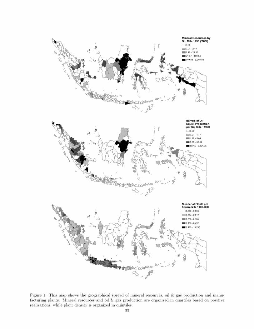
Number of Plants perSquare Mile 1990-2009

0.000 - 0.0030.004 - 0.0120.013 - 0.1040.105 - 0.4920.493 - 15.737

Barrels of OilEquiv. Productionper Sq. Mile ~1990

0.000.01 - 1.171.18 - 5.045.05 - 58.1458.15 - 2,301.35

Mineral Resources bySq. Mile 1990 ('000t)

0.000.01 - 2.442.45 - 21.3621.37 - 149.84149.85 - 3,946.04

Figure 1: This map shows the geographical spread of mineral resources, oil & gas production and manu-facturing plants. Mineral resources and oil & gas production are organized in quartiles based on positiverealizations, while plant density is organized in quintiles.

33

log(100)log(200)log(400)

1990 1995 2000 2005 2010

Coal

1990 1995 2000 2005 2010

Copper

1990 1995 2000 2005 2010

Gold

1990 1995 2000 2005 2010

Silver

log(100)log(200)log(400)

1990 1995 2000 2005 2010

Tin

1990 1995 2000 2005 2010

Nickel

1990 1995 2000 2005 2010

Aluminum

1990 1995 2000 2005 2010

Iron Ore

log(100)log(200)log(400)

1990 1995 2000 2005 2010

Cobalt

1990 1995 2000 2005 2010

Diamonds

1990 1995 2000 2005 2010

Uranium

1990 1995 2000 2005 2010

Manganese

log(100)log(200)log(400)

1990 1995 2000 2005 2010

Zirconium

1990 1995 2000 2005 2010

Oil

Log Prices 1990-2010

Figure 2: This figure shows the log of the indexed price series (P1990 = log(100)) of all minerals that werefound in Indonesia in 1990. Minerals are arranged from top left to bottom right based on their share in totalmineral resources. The oil price is at the bottom right. See Online Appendix OA5 for the individual priceseries sources.

34

Tab

le1:

Res

ourc

ein

ten

sity

an

dex

tract

ion

tech

niq

ues

by

pro

vin

ce

Pro

vin

ceD

istr

icts

Min

ing

Dis

tric

tsoil

&gas

Dis

tric

ts

Min

eral

Ore

Res

ou

rces

/A

rea

1990

Min

ing

tech

niq

ues

Min

erals

oil

&gas

Pro

du

ctio

n/

Are

a,

1990

Bal

i8

00

00

Ben

gku

lu4

10

0.4

1U

G,O

PG

old

,S

ilve

r0

Cen

tral

Jav

a35

20

0.6

4O

PIr

on

Ore

,M

an

gan

ese

0C

entr

alK

alim

anta

n6

30

0.9

1O

P,P

lace

rA

lum

inu

m,

Gold

,S

ilve

r,Z

irco

niu

m0

Cen

tral

Su

law

esi

41

00.6

1O

PC

op

per

0D

ista

Ace

h10

12

27.3

7O

PC

op

per

23.2

8D

IY

ogya

kart

a5

10

227.9

5O

P,P

lace

rIr

on

Ore

0D

KI

Jak

arta

50

10

197.1

2E

ast

Jav

a37

13

0.1

0O

PIr

on

Ore

0.4

0E

ast

Kal

iman

tan

63

4152.3

1U

G,O

PC

oal,

Gold

,S

ilve

r335.8

6E

ast

Nu

saT

engg

ara

120

00

0Ir

ian

Jay

a(P

apu

a)9

21

41.8

5U

G,O

PC

op

per

,G

old

,N

icke

l,S

ilve

r0.2

1Jam

bi

60

30

1.5

8L

amp

un

g4

11

0.0

9U

G,O

PG

old

26.0

8M

alu

ku

42

18.2

1O

PC

op

per

,G

old

,N

icke

l,S

ilve

r0.0

6N

orth

Su

law

esi

63

043.8

6O

PC

op

per

,G

old

0N

orth

Su

mat

ra17

02

00.4

4R

iau

72

55.0

4O

PA

lum

iniu

m,

Coal,

Tin

10.4

0S

outh

Kal

iman

tan

103

1591.3

4O

P,P

lace

rC

oal,

Dia

mon

ds

0.2

3S

outh

Su

law

esi

231

08.1

9O

PN

icke

l,C

ob

alt

0S

outh

Su

mat

ra9

35

286.6

8U

G,O

PC

oal,

Gold

,S

ilve

r,T

in127.7

3S

outh

east

Su

law

esi

41

02.0

0O

PN

icke

l0

Wes

tJav

a24

35

1.2

1U

G,O

PG

old

,M

an

gan

ese,

Sil

ver

245.1

3W

est

Kal

iman

tan

73

05.5

9U

G,O

PA

lum

inu

m,

Ura

niu

m0

Wes

tN

usa

Ten

ggar

a6

10

205.5

0O

PG

old

,C

op

per

0W

est

Su

mat

ra13

13

6.6

1U

G,O

PC

oal

20.1

7T

OT

AL

281

3937

Tab

le1

pro

vid

esd

escr

ipti

ves

stat

isti

cson

min

eral

reso

urc

es,

oil

an

dgas

pro

du

ctio

nin

ten

sity

an

dm

iner

al

reso

urc

eex

tract

ion

tech

niq

ues

atth

ep

rovin

cele

vel

.M

iner

al

Ore

Res

ou

rces

/A

rea

1990

ind

icate

sm

iner

al

ore

reso

urc

esp

erd

istr

ict

inth

ou

san

dto

ns

per

squ

are

mil

ein

1990

.oil

&ga

sP

rodu

ctio

n/

Are

a1990

ind

icate

sth

ep

rod

uct

ion

of

oil

an

dgas

per

squ

are

mil

ein

term

sof

barr

els

of

oil

equ

ivale

nt,

aro

un

dth

eye

ar19

90.

Min

ing

Tec

hn

iqu

esin

dic

ate

sth

eex

tract

ion

tech

niq

ues

that

wer

eap

plied

on

min

eral

reso

urc

esu

nd

erd

evel

op

men

tas

of

1990

orte

chn

iqu

esp

lan

ned

tob

eap

pli

edon

reso

urc

esth

at

had

bee

nd

isco

vere

db

ut

wer

en

ot

yet

bei

ng

dev

elop

edin

1990.

UG

stan

ds

for

un

der

grou

nd

,O

Pfo

rop

en-p

itan

dP

lace

rfo

rP

lace

rm

inin

g.

Min

erals

are

those

that

wer

eex

tract

ed,

or

pla

nn

edto

be

extr

act

edfr

om

dis

cove

red

dep

osit

s,as

of19

90.

Ban

gka

an

dB

elit

un

gare

trea

ted

as

on

ed

istr

ict;

see

Onli

ne

Ap

pen

dix

OA

2fo

rd

etail

s.

35

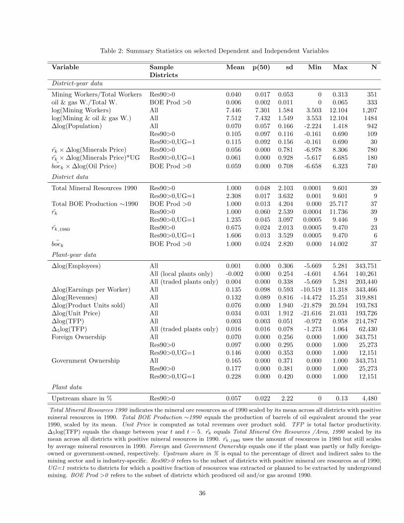
Table 2: Summary Statistics on selected Dependent and Independent Variables

Variable Sample Mean p(50) sd Min Max NDistricts

District-year data

Mining Workers/Total Workers Res90>0 0.040 0.017 0.053 0 0.313 351oil & gas W./Total W. BOE Prod >0 0.006 0.002 0.011 0 0.065 333log(Mining Workers) All 7.446 7.301 1.584 3.503 12.104 1,207log(Mining & oil & gas W.) All 7.512 7.432 1.549 3.553 12.104 1484∆log(Population) All 0.070 0.057 0.166 -2.224 1.418 942

Res90>0 0.105 0.097 0.116 -0.161 0.690 109Res90>0,UG=1 0.115 0.092 0.156 -0.161 0.690 30

rk ×∆log(Minerals Price) Res90>0 0.056 0.000 0.781 -6.978 8.306 780rk ×∆log(Minerals Price)*UG Res90>0,UG=1 0.061 0.000 0.928 -5.617 6.685 180

˜boek ×∆log(Oil Price) BOE Prod >0 0.059 0.000 0.708 -6.658 6.323 740

District data

Total Mineral Resources 1990 Res90>0 1.000 0.048 2.103 0.0001 9.601 39Res90>0,UG=1 2.308 0.017 3.632 0.001 9.601 9

Total BOE Production ∼1990 BOE Prod >0 1.000 0.013 4.204 0.000 25.717 37rk Res90>0 1.000 0.060 2.539 0.0004 11.736 39

Res90>0,UG=1 1.235 0.045 3.097 0.0005 9.446 9rk,1980 Res90>0 0.675 0.024 2.013 0.0005 9.470 23

Res90>0,UG=1 1.606 0.013 3.529 0.0005 9.470 6˜boek BOE Prod >0 1.000 0.024 2.820 0.000 14.002 37

Plant-year data

∆log(Employees) All 0.001 0.000 0.306 -5.669 5.281 343,751All (local plants only) -0.002 0.000 0.254 -4.601 4.564 140,261All (traded plants only) 0.004 0.000 0.338 -5.669 5.281 203,440

∆log(Earnings per Worker) All 0.135 0.098 0.593 -10.519 11.318 343,466∆log(Revenues) All 0.132 0.089 0.816 -14.472 15.251 319,881∆log(Product Units sold) All 0.076 0.000 1.940 -21.879 20.594 193,783∆log(Unit Price) All 0.034 0.031 1.912 -21.616 21.031 193,726∆log(TFP) All 0.003 0.003 0.051 -0.972 0.958 214,787∆5log(TFP) All (traded plants only) 0.016 0.016 0.078 -1.273 1.064 62,430Foreign Ownership All 0.070 0.000 0.256 0.000 1.000 343,751

Res90>0 0.097 0.000 0.295 0.000 1.000 25,273Res90>0,UG=1 0.146 0.000 0.353 0.000 1.000 12,151

Government Ownership All 0.165 0.000 0.371 0.000 1.000 343,751Res90>0 0.177 0.000 0.381 0.000 1.000 25,273Res90>0,UG=1 0.228 0.000 0.420 0.000 1.000 12,151

Plant data

Upstream share in % Res90>0 0.057 0.022 2.22 0 0.13 4,480

Total Mineral Resources 1990 indicates the mineral ore resources as of 1990 scaled by its mean across all districts with positivemineral resources in 1990. Total BOE Production ∼1990 equals the production of barrels of oil equivalent around the year1990, scaled by its mean. Unit Price is computed as total revenues over product sold. TFP is total factor productivity.∆5log(TFP) equals the change between year t and t − 5. rk equals Total Mineral Ore Resources /Area, 1990 scaled by itsmean across all districts with positive mineral resources in 1990. rk,1980 uses the amount of resources in 1980 but still scalesby average mineral resources in 1990. Foreign and Government Ownership equals one if the plant was partly or fully foreign-owned or government-owned, respectively. Upstream share in % is equal to the percentage of direct and indirect sales to themining sector and is industry-specific. Res90>0 refers to the subset of districts with positive mineral ore resources as of 1990;UG=1 restricts to districts for which a positive fraction of resources was extracted or planned to be extracted by undergroundmining. BOE Prod >0 refers to the subset of districts which produced oil and/or gas around 1990.

36

Table 3: The labour intensity of different types of natural resource extraction

Dependent variable ln(# Mining and oil & gas Workers)

(1) (2) (3) (4)

Total Mineral Resources 1990 0.39*** 0.30*** 0.40*** 0.18*(0.086) (0.107) (0.098) (0.092)

Total BOE Production ∼1990 0.07*** 0.05** 0.07*** -0.01(0.018) (0.023) (0.021) (0.023)

Underground Mining 1.07**(0.505)

100% Underground Mining 2.45*** 1.96***(0.185) (0.236)

Underground & Open-Pit Mining -0.05 1.17*(0.566) (0.691)

Year FE Yes Yes Yes YesProvince FE No No No YesObservations 1,484 1,484 1,484 1,484adj. R2 0.119 0.137 0.163 0.416

In this table we analyse whether underground mining is more labour-intensive than other types of mining. The sample period is 2007-2015, theunit of observation is a district-year. The dependent variable is the logof an approximation of the number of mining and oil & gas workers (seeOnline Appendix OA7). Total Mineral Resources 1990 equals mineral oreresources as of 1990 scaled by its mean across all districts with positivemineral resources in 1990. Total BOE Production ∼1990 equals theproduction of barrels of oil equivalent around the year 1990, scaled byits mean for producing districts. Underground Mining is a dummy thatequals one if at least one of the 1990 deposits in the district was operatedor planned to be operated by underground mining. 100% UndergroundMining is a dummy that equals one if all 1990 deposits were operated orplanned to be operated by underground mining. Underground & Open-Pit Mining is a dummy that equals one if both underground and open-pit mining was applied or planned to be applied in order to extractthe district’s 1990 mineral resources. Standard errors in parentheses areclustered at the district level. *** Significant at 1% level; ** Significantat 5% level; * Significant at 10% level.

37

Table 4: Mineral price shocks and immigration into mineral-rich districts

Dependent variable ∆5 ln(Populationt)

(1) (2) (3) (4)

Mineral Resources 1990 × W1∆ln(Minerals Price) 0.044** 0.000(0.021) (0.035)

Mineral Resources 1990 × W1∆ln(Minerals Price) × Underground 0.060*(0.035)

BOE Production ∼1990 × W1∆ln(Oil Price) -0.019 -0.019(0.037) (0.037)

Mineral Resources 1990 × W2∆ln(Minerals Price) -0.030(0.018)

Mineral Resources 1990 × W2∆ln(Minerals Price) × Underground 0.082***(0.027)

BOE Production ∼1990 × W2∆ln(Oil Price) -0.018(0.028)

Mineral Resources 1990 × ∆5Minerals Price 0.000(0.007)

Mineral Resources 1990 × ∆5Minerals Price × Underground 0.012*(0.007)

BOE Production ∼1990 × ∆5ln(Oil Price) -0.004(0.007)

Mineral Resources 1990 -0.005 0.001 0.005 0.001(0.003) (0.005) (0.004) (0.005)

BOE Production ∼1990 0.003 0.003 0.005 0.003(0.004) (0.004) (0.004) (0.004)

Population 1990 -0.029*** -0.029*** -0.029*** -0.029***(0.009) (0.009) (0.009) (0.009)

Observations 939 939 939 939adj. R2 0.040 0.040 0.040 0.040

Marginal effect of mining boom for underground mining=1 0.061*** 0.052** 0.012***(0.018) (0.025) (0.003)

This table shows the effect of global mineral price shocks on immigration into mineral-rich districts versusdistricts with relatively smaller or no mineral resources. Conceptually, the underlying specification is equa-tion (11), while in practice we adjust the specification in terms of timing, since population is only recordedevery five years. The sample period is 1990-2010. The unit of observation is a district-period; the depen-dent variable is the change in log total population across the periods 1990-1995, 1995-2000, 2000-2005 and2005-2010. Mineral Resources 1990 equals mineral ore resources per square mile as of 1990 scaled by itsmean across all districts with positive mineral resources in 1990. Total BOE Production ∼1990 equals theproduction of barrels of oil equivalent per square mile around the year 1990, scaled by its mean for producingdistricts. We also include the interaction of Mineral Resources 1990 with the weighted change in the logprice of minerals present in the district in 1990. The weight of each mineral equals its share in total 1990mineral resources. We capture minerals price shocks over the five-year periods in different ways. In columns1 and 2, W1 is the simple average of the five annual price shocks. In column 3, the weight W2 of a givenprice decreases as it lies further in the past; in particular, the weights are 0.3, 0.25, 0.2, 0.15 and 0.1 forperiods t through (t − 4). In column 4, we simply compute the price shock as the difference between thecurrent district-specific minerals price and its five-year lag. Underground Mining equals one if at least oneof the 1990 deposits in the district was operated or planned to be operated by underground mining. Themarginal effect at the bottom of the table equals the sum of the first two coefficients in the given column.All specifications contain dummies for the years 2000, 2005 and 2010. Standard errors in parentheses areclustered at the district level. ***Significant at 1% level; **Significant at 5% level; *Significant at 10% level.

38

Table 5: Mineral price shocks and plant-level manufacturing earnings per worker

Dependent variable → ∆ln(Average earnings per worker)

Sample → All Plants All Plants Non-Exporters ExportersLocal Goods

ProducersTraded Goods

Producers

(1) (2) (3) (4) (5) (6)

Mineral Resources 1990× ∆ln(Minerals Price)

0.022 -0.012 0.019* -0.043 0.018* -0.042(0.020) (0.021) (0.010) (0.028) (0.011) (0.026)

Mineral Resources 1990× ∆ln(Minerals Price) ×Underground Mining

0.071*** 0.093*** 0.049* 0.094*** 0.047*(0.021) (0.011) (0.028) (0.011) (0.026)

BOE Production ∼1990× ∆ln(Oil Price)

-0.002 -0.002 -0.001 -0.004 -0.005 -0.001(0.003) (0.003) (0.002) (0.005) (0.005) (0.003)

Mineral Resources 1990 0.000 0.002 -0.003 0.007*** -0.004 0.007***(0.002) (0.003) (0.004) (0.003) (0.004) (0.003)

BOE Production ∼1990 -0.000 -0.000 -0.000 0.000 0.001 -0.001(0.001) (0.001) (0.001) (0.001) (0.001) (0.001)

Underground Mining 0.001 0.007** -0.004 0.004 -0.001(0.002) (0.003) (0.004) (0.003) (0.003)

Mineral Resources 1990× Underground Mining

-0.005* -0.003 -0.006** -0.001 -0.007**(0.003) (0.004) (0.003) (0.004) (0.003)

Observations 343,466 343,466 224,078 119,250 140,167 203,249# Plants 49,836 49,836 35,851 13,985 23,101 29,650adj. R2 0.034 0.034 0.035 0.037 0.032 0.036

Marginal effect ofmining boom for under-ground mining=1

0.059*** 0.112*** 0.006 0.112*** 0.005(0.003) (0.004) (0.005) (0.004) (0.005)

This table shows the effect of global mineral price shocks on the change in earnings per worker in different groupsof manufacturing plants in mineral-rich districts versus districts with relatively smaller or no mineral resources.The underlying specification is equation (11). The sample contains all formal manufacturing plants with at least20 employees for the years 1990-2009. The dependent variable is the annual change in log average earnings perworker at each plant. We interact the plant’s home district mineral resources as of 1990 with a time-varying,district-specific weighted mineral price shock. The weight of each mineral’s price shock equals its share in total1990 resources. Mineral Resources 1990 equals mineral ore resources per square mile as of 1990 scaled by itsmean across all districts with positive mineral resources in 1990 (rk in equation (11)). Total BOE Production∼1990 equals the production of barrels of oil equivalent per square mile around the year 1990, scaled by itsmean for producing districts ( ˜boek in equation (11)). Underground Mining is a dummy that equals one if atleast one of the 1990 mineral deposits in the district was operated or planned to be operated by undergroundmining (which typically requires more labour than open-pit or other types of mines). The marginal effect atthe bottom of the table equals the sum of the first two coefficients in the given column. We classify a plant asexporter if it exported a positive share of its output in at least one year during the sample period. The group‘Local Goods Producers’ includes all plants which operate in a four-digit industry whose average U.S. distanceelasticity is above the industry median and are non-exporters. The plants in the opposite category are thus eitherinternational exporters or have a relatively low distance elasticity according to our measure. All specificationscontain four-digit industry-times-year fixed effects. The difference-in-difference specification absorbs plant-fixedeffects. Standard errors in parentheses are clustered at the district level. ***Significant at 1% level; **Significantat 5% level; * Significant at 10% level.

39

Table 6: Mineral price shocks and plant-level manufacturing employment

Dependent variable → ∆ln(# Employees)

Sample → All Plants All Plants Non-Exporters ExportersLocal Goods


Producers

(1) (2) (3) (4) (5) (6)

Mineral Resources 1990× ∆ln(Minerals Price)

0.020* 0.035*** 0.021*** 0.048** 0.021*** 0.048**(0.010) (0.010) (0.007) (0.022) (0.007) (0.022)

Mineral Resources 1990× ∆ln(Minerals Price) ×Underground Mining

-0.033*** -0.006 -0.057** -0.006 -0.056***(0.010) (0.007) (0.022) (0.007) (0.022)

BOE Production ∼1990× ∆ln(Oil Price)

-0.001 -0.001 0.000 -0.001 0.002 -0.002(0.001) (0.001) (0.001) (0.002) (0.002) (0.002)

Mineral Resources 1990 0.001 0.000 0.006* -0.004 0.006* -0.005(0.001) (0.002) (0.003) (0.004) (0.003) (0.004)

BOE Production ∼1990 0.002*** 0.002*** 0.001*** 0.003*** 0.001 0.003***(0.000) (0.000) (0.000) (0.000) (0.001) (0.000)

Underground Mining 0.010*** 0.008*** 0.009*** 0.007*** 0.011***(0.002) (0.001) (0.003) (0.001) (0.002)

Mineral Resources 1990× Underground Mining

-0.000 -0.003 0.003 -0.003 0.003(0.002) (0.003) (0.004) (0.003) (0.004)

Observations 343,751 343,751 224,235 119,378 140,261 203,440# Plants 49,851 49,851 35,864 13,987 23,106 29,662adj. R2 0.016 0.016 0.016 0.017 0.015 0.017

Marginal effect ofmining boom forunderground mining=1

0.003* 0.015*** -0.009*** 0.015*** -0.009***(0.002) (0.002) (0.002) (0.002) (0.002)

This table shows the effect of global mineral price shocks on the change in employment of different groups ofmanufacturing plants in mineral-rich districts versus districts with relatively smaller or no mineral resources. Theunderlying specification is equation (11). The sample contains all formal manufacturing plants with at least 20employees, over the period 1990-2009. The dependent variable is the annual change in log number of workers ateach plant. See Table 5 for the description of independent variables and column labels. The marginal effect atthe bottom of the table equals the sum of the first two coefficients in the given column. All specifications containfour-digit industry-times-year fixed effects. The difference-in-difference specification absorbs plant-fixed effects.Standard errors in parentheses are clustered at the district level. ***Significant at 1% level; **Significant at 5%level; * Significant at 10% level.

40

Table 7: Mineral price shocks and plant-level revenues, sales and prices

Sample → All PlantsLocal Goods


Producers

Panel A ∆ln(Revenues)

(1) (2) (3)

Mineral Resources 1990 × ∆ln(Minerals Price) 0.019 0.041 0.001(0.018) (0.037) (0.024)

Mineral Resources 1990 × ∆ln(Minerals Price) × Underground Mining 0.067*** 0.112*** 0.010(0.018) (0.037) (0.025)

BOE Production ∼1990 × ∆ln(Oil Price) 0.003** 0.004 0.002(0.002) (0.002) (0.003)

Observations 319,881 135,132 184,701adj. R2 0.033 0.038 0.034

Marginal effect of mining boom for underground mining=1 0.085*** 0.153*** 0.012**(0.004) (0.006) (0.006)

Panel B ∆ln(Number of Product Units sold)

(4) (5) (6)

Mineral Resources 1990 × ∆ln(Minerals Price) 0.049 0.032 0.063(0.045) (0.036) (0.053)

Mineral Resources 1990 × ∆ln(Minerals Price) × Underground Mining -0.024 -0.025 -0.024(0.047) (0.036) (0.058)

BOE Production ∼1990 × ∆ln(Oil Price) 0.011 0.010 0.008(0.016) (0.008) (0.026)


Marginal effect of mining boom for underground mining=1 0.025* 0.007 0.039(0.014) (0.008) (0.025)

Panel C ∆ln(Unit Price)

(7) (8) (9)

Mineral Resources 1990 × ∆ln(Minerals Price) -0.006 0.032 -0.039(0.043) (0.047) (0.041)

Mineral Resources 1990 × ∆ln(Minerals Price) × Underground Mining 0.072 0.121** 0.012(0.045) (0.047) (0.048)

BOE Production ∼1990 × ∆ln(Oil Price) -0.016* -0.011 -0.018(0.010) (0.009) (0.020)


Marginal effect of mining boom for underground mining=1 0.066*** 0.153*** -0.027(0.014) (0.010) (0.026)

This table shows the effect of global mineral price shocks on the annual change in log plant-level revenues, productssold and unit prices, of different groups of manufacturing plants in mineral-rich districts versus districts with relativelysmaller or no mineral resources. The underlying specification is equation (11). The sample contains the entirepopulation of manufacturing plants with at least 20 employees for the years 1990-2009 in Panel A, and 1998-2009 inPanels B and C, due to data availability. Both revenues and the number of products sold are directly reported bythe plant in the census. To compute the unit price (Panel C), we compute the ratio of the two. See Table 5 for thedescription of independent variables and column labels. The marginal effect at the bottom of the table equals the sumof the first two coefficients in the given column. All specifications contain four-digit industry-times-year fixed effects.The difference-in-difference specification absorbs plant-fixed effects. We always include Mineral Resources 1990,Underground Mining, their interaction and BOE Production ∼1990, but do not report their coefficients. Standarderrors in parentheses are clustered at the district level. *** Significant at 1% level; ** Significant at 5% level; *Significant at 10% level. 41

Table 8: Mineral price shocks and plant-level Total Factor Productivity (TFP)

Dependent variable → ∆ln(TFP) ∆5ln(TFP)

Sample → All PlantsLocal Goods



Producers

(1) (2) (3) (4)

Mineral Resources 1990 × ∆ln(Minerals Price) -0.001 0.001 -0.004*(0.001) (0.002) (0.002)

Mineral Resources 1990 × ∆ln(Minerals Price)× Underground Mining

0.006*** 0.006** 0.005**(0.001) (0.002) (0.002)

BOE Production ∼1990 × ∆ln(Oil Price) -0.000 0.001** -0.001(0.000) (0.000) (0.001)

Mineral Resources 1990 × W1∆ln(Minerals Price) -0.001(0.017)

Mineral Resources 1990 × W1∆ln(Minerals Price)× Underground Mining

0.021(0.023)

BOE Production ∼1990 × W1∆ln(Oil Price) 0.001(0.004)

Observations 214,787 90,126 124,605 62,430adj. R2 0.088 0.104 0.087 0.101

Marginal effect of mining boom for underground mining=1 0.004*** 0.007*** 0.001 0.021(0.000) (0.000) (0.001) (0.015)

This table shows the effect of global mineral price shocks on the annual change plant-level total factor productivity (TFP)of different groups of manufacturing plants in mineral-rich districts versus districts with relatively smaller or no mineralresources. Our sample contains the entire population of manufacturing plants with at least 20 employees. In columns 1-3,the dependent variable is the change in TFP between t and t−1. The underlying specification is equation (11), the sampleperiod 1990-2009. See Table 5 for the description of independent variables in columns 1-3. In column 4, the dependentvariable is the change in TFP between t and t− 5. On the right-hand side, the price change is not measured between tand t− 1 as in columns 1-3, but as the simple average price change across t and t− 1, t− 1 and t− 2, t− 2 and t− 3, t− 3and t− 4 and t− 4 and t− 5. The sample period is therefore 1995-2009 instead of 1990-2009. The marginal effect at thebottom of the table equals the sum of the first two coefficients in the given column. All specifications contain four-digitindustry-times-year fixed effects. The difference-in-difference specification absorbs plant-fixed effects. We always includeMineral Resources 1990, Underground Mining, their interaction and BOE Production ∼1990, but do not report theircoefficients. Standard errors in parentheses are clustered at the district level. ***Significant at 1% level; **Significant at5% level; * Significant at 10% level.

42

Tab

le9:

Addit

ional

resu

lts:

Reg

ional

spillo

vers

and

reven

ue

shari

ng

Dep

enden

tva

riab

le→

∆ln

(#E

mplo

yees

)

Bas

elin

eB

oom

snea

rby

Boom

sin

sam

epro

vin

ceB

oom

snea

rby,

aft

er19

99

Boom

sin

sam

epro

vin

ce,

afte

r19

99

Tw

o-w

aycl

ust

erin

g

(1)

(2)

(3)

(4)

(5)

(6)

Min

eral

Res

ourc

es19

90×

∆ln

(Min

eral

sP

rice

)0.0

35∗∗∗

0.03

4∗∗∗

0.0

33∗∗∗

0.03

2∗∗

0.03

2∗∗

0.03

5∗∗∗

(0.0

10)

(0.0

11)

(0.0

09)

(0.0

14)

(0.0

13)

(0.0

03)

Min

eral

Res

ourc

es19

90×

∆ln

(Min

eral

sP

rice

)×

Under

gro

und

Min

ing

-0.0

33∗∗∗

-0.0

32∗∗∗

-0.0

31∗∗∗

-0.0

36∗∗∗

-0.0

35∗∗∗

-0.0

33∗∗∗

(0.0

10)

(0.0

11)

(0.0

09)

(0.0

14)

(0.0

13)

(0.0

02)

BO

EP

roduct

ion∼

1990×

∆ln

(Oil

Pri

ce)

-0.0

01-0

.001

-0.0

01

-0.0

01-0

.001

-0.0

01(0

.001)

(0.0

01)

(0.0

01)

(0.0

01)

(0.0

01)

(0.0

01)

Nei

ghb

ours

’M

iner

alR

esou

rces

1990×

∆ln

(Nei

ghb

ours

’M

iner

als

Pri

ce)

0.00

50.

003

(0.0

22)

(0.0

22)

Nei

ghb

ours

’M

iner

alR

esou

rces

1990×

∆ln

(Nei

ghb

ours

’M

iner

als

Pri

ce)

×N

eigh

bou

rs’

Under

grou

nd

Min

ing

0.001

0.00

6(0

.024)

(0.0

24)

Nei

ghb

ours

’B

OE

Pro

duct

ion∼

1990×

∆ln

(Oil

Pri

ce)

-0.0

01

0.00

1(0

.001)

(0.0

01)

Oth

ersP

rov

Min

eral

Res

ourc

es19

90×

∆ln

(Oth

ersP

rov

Min

eral

sP

rice

)0.0

030.

002

(0.0

03)

(0.0

03)

Oth

ersP

rov

BO

EP

roduct

ion∼

1990×

∆ln

(Oil

Pri

ce)

-0.0

02

-0.0

01

(0.0

01)

(0.0

02)

Obse

rvat

ions

343,

751

342,

065

343

,751

196

,189

196

,935

343

,751

adj.R

20.0

160.0

150.

016

0.00

40.

004

0.01

6

Marg

inal

effec

tof

min

ing

boom

for

un

der

grou

nd

min

ing=

10.0

03∗

0.0

03

0.0

03∗

-0.0

04∗

-0.0

04∗∗

0.0

03

(0.0

02)

(0.0

02)

(0.0

02)

(0.0

02)

(0.0

02)

(0.0

04)

This

table

show

sth

ere

sult

sof

robust

nes

sch

ecks

of

the

base

line

resu

lt.

To

faci

lita

teth

eco

mpari

son,

colu

mn

1dis

pla

ys

the

resu

lts

of

our

base

line

spec

ifica

tion

(Tab

le6,

colu

mn

1).

Inco

lum

n2,

we

contr

olfo

rm

inin

gb

oom

s/bust

sin

nei

ghb

ouri

ng

dis

tric

tsw

her

ew

etr

eat

all

nei

ghb

ours

ason

edis

tric

tan

dco

mpute

its

min

eral

reso

urc

esan

dpri

cesh

ock

anal

ogou

sly

toth

esi

ngl

e-dis

tric

tca

se.

Inco

lum

n3,

we

contr

olfo

rth

eav

erag

em

inin

gb

oom

/bust

inoth

erdis

tric

tsof

the

sam

epro

vin

ce.

Col

um

ns

4an

d5

rep

eat

the

spec

ifica

tions

ofco

lum

ns

2an

d3,

resp

ecti

vely

,es

tim

ated

over

the

per

iod

200

0-20

09.

Sta

ndard

erro

rsin

par

enth

eses

are

clust

ered

atth

edis

tric

tle

vel,

exce

pt

inco

lum

n6

wher

ew

ecl

ust

erat

both

the

dis

tric

tand

year.

The

diff

eren

ce-i

n-d

iffer

ence

spec

ifica

tion

abso

rbs

pla

nt-

fixed

effec

ts.

We

alw

ays

incl

ude

all

com

bin

atio

ns

of

inte

ract

edte

rms,

but

do

not

rep

ort

thei

rco

effici

ents

.∗∗∗

Sig

nifi

cant

at1%

leve

l;∗∗

Sig

nifi

cant

at5%

leve

l;∗

Sig

nifi

cant

at10

%le

vel.

43

Tab

le10

:R

obust

nes

sI:

198

0en

dow

men

ts,

indust

rysw

itch

ers,

owner

ship

and

upst

ream

pla

nts

Dep

enden

tva

riab

le→

∆ln

(#E

mplo

yee

s)

Bas

elin

eR

esou

rces

1980

No

indust

rysw

itch

ers

Ow

ner

ship

Con

trol

sU

pst

ream

Con

trol

s

(1)

(2)

(3)

(4)

(5)

Min

eral

Res

ourc

es19

90×

∆ln

(Min

eral

sP

rice

)0.0

35**

*0.

037

***

0.0

25**

*0.0

26**

*(0

.010

)(0

.011

)(0

.004

)(0

.010

)M

iner

alR

esou

rces

1990×

∆ln

(Min

eral

sP

rice

)×

Under

gro

und

Min

ing

-0.0

33***

-0.0

30**

*-0

.024

***

-0.0

19**

(0.0

10)

(0.0

11)

(0.0

04)

(0.0

10)

BO

EP

roduct

ion∼

1990×

∆ln

(Oil

Pri

ce)

-0.0

01

-0.0

01-0

.002

-0.0

01

-0.0

00(0

.001

)(0

.001

)(0

.001

)(0

.001

)(0

.001

)M

iner

alR

esou

rces

1980×

∆ln

(Min

eral

sP

rice

)0.

066*

**(0

.009

)M

iner

alR

esou

rces

1980×

∆ln

(Min

eral

sP

rice

)×

Under

gro

und

Min

ing

-0.0

64**

*(0

.009

)M

iner

alR

esou

rces

1990×

∆ln

(Min

eral

sP

rice

)×

Fore

ign

Ow

ner

ship

(t-1

)0.

123*

*(0

.056

)M

iner

alR

esou

rces

1990×

∆ln

(Min

eral

sP

rice

)×

Fore

ign

Ow

ner

ship

(t-1

)×

Under

ground

Min

ing

-0.0

15(0

.058

)M

iner

alR

esou

rces

1990×

∆ln

(Min

eral

sP

rice

)×

Gov

ernm

ent

Ow

ner

ship

(t-1

)-0

.033

(0.0

27)

Min

eral

Res

ourc

es19

90×

∆ln

(Min

eral

sP

rice

)×

Gov

ernm

ent

Ow

ner

ship

(t-1

)×

Under

ground

Min

ing

-0.0

52*

(0.0

29)

Min

eral

Res

ourc

es19

90×

∆ln

(Min

eral

sP

rice

)×

Upst

ream

share>

50p

ctl

0.01

9(0

.039

)M

iner

alR

esou

rces

1990×

∆ln

(Min

eral

sP

rice

)×

Upst

ream

shar

e>

50p

ctl×

Under

grou

nd

Min

ing

-0.0

21(0

.038)

Obse

rvat

ions

343,7

51

343,

751

230,

353

343,7

5134

3,82

6ad

j.R

20.

016

0.016

0.01

40.

016

0.00

9

Marg

inal

effec

tof

min

ing

boom

for

un

der

grou

nd

min

ing=

10.0

03∗

0.0

03∗

0.0

07∗∗∗

see

0.0

07∗∗∗

(0.0

02)

(0.0

01)

(0.0

02)

belo

w(0

.001)

Marg

inal

effec

tof

aca

pit

al-

inte

nsi

vebo

om

on

:D

om

esti

cpri

vate

pla

nt:

0.0

25∗∗∗

(0.0

04)

;F

ore

ign

-ow

ned

pla

nt:

0.1

48∗∗

(0.0

59)

;G

ove

rnm

ent-

ow

ned

pla

nt:

-0.0

08

(0.0

24)

Marg

inal

effec

tof

ala

bou

r-in

ten

sive

boom

on

:D

om

esti

cpri

vate

pla

nt:

0.0

01

(0.0

02)

;F

ore

ign

-ow

ned

pla

nt:

0.1

09∗∗

(0.0

15)

;G

ove

rnm

ent-

ow

ned

pla

nt:

-0.0

84∗∗∗

(0.0

14)

This

table

show

sth

ere

sult

sof

robust

nes

sch

ecks

of

the

base

line

resu

lt.

Col

um

n2

mea

sure

sen

dow

men

tsin

198

0.

Col

um

n3

dro

ps

all

pla

nts

that

ever

chan

ge

four-

dig

itin

dust

ry.

Inco

lum

n5

Fore

ign

and

Gove

rnm

ent

Ow

ner

ship

are

pla

nt-

and

year-

spec

ific

dum

mie

sw

hic

heq

uals

one

ifth

epla

nt

was

par

tly

orfu

lly

fore

ign-o

wned

orgo

vern

men

tow

ned

,re

spec

tive

ly.

Inco

lum

n6

Upst

ream

share>

50

pctl

equals

one

ifth

ein

dust

ryse

lls

anab

ove

med

ian

shar

eto

the

min

ing

sect

or.

All

spec

ifica

tions

conta

info

ur-

dig

itin

dust

ry-t

imes

-yea

rfixed

effec

ts.

The

diff

eren

ce-i

n-d

iffer

ence

spec

ifica

tion

abso

rbs

pla

nt-

fixed

effec

ts.

We

alw

ays

incl

ude

all

com

bin

atio

ns

of

inte

ract

edte

rms,

but

do

not

rep

ort

thei

rco

effici

ents

.Sta

ndar

der

rors

inpar

enth

eses

are

clust

ered

at

the

dis

tric

tle

vel.∗∗∗

Sig

nifi

cant

at

1%le

vel;∗∗

Sig

nifi

cant

at5%

leve

l;∗

Sig

nifi

cant

at10

%le

vel.

44

Tab

le11

:R

obust

nes

sII

:m

ark

etp

ower

,m

iner

al-s

pec

ific

effec

ts,

dec

entr

aliza

tion

,and

resc

alin

g

Dep

enden

tva

riab

le→

∆ln

(#E

mplo

yees

)∆

ln(E

arn

ings

per

work

er)

Base

line

Excl

udin

gT

in&

Nic

kel

Sam

eM

iner

al

Aft

er1999

FE

AK

201

7sc

aling

AK

201

7sc

alin

g

(1)

(2)

(3)

(4)

(5)

(6)

Min

eral

Res

ourc

es19

90×

∆ln

(Min

eral

sP

rice

)0.

035∗∗∗

0.0

35∗∗∗

0.0

34∗∗∗

0.036∗∗∗

(0.0

10)

(0.0

10)

(0.0

10)

(0.0

10)

Min

eral

Res

ourc

es19

90×

∆ln

(Min

erals

Pri

ce)×

Under

gro

und

Min

ing

-0.0

33∗∗∗

-0.0

33∗∗∗

-0.0

31∗∗∗

-0.0

33∗∗∗

(0.0

10)

(0.0

10)

(0.0

10)

(0.0

10)

BO

EP

roduct

ion∼

199

0×

∆ln

(Oil

Pri

ce)

-0.0

01-0

.001

-0.0

01

-0.0

01

(0.0

01)

(0.0

01)

(0.0

01)

(0.0

01)

Min

eral

Res

ourc

es19

90(A

K20

17)×

∆ln

(Min

erals

Pri

ce)

0.088∗∗∗

-0.0

29

(0.0

24)

(0.0

52)

Min

eral

Res

ourc

es199

0(A

K20

17)×

∆ln

(Min

eral

sP

rice

)×

Under

ground

Min

ing

-0.0

82∗∗∗

0.1

77∗∗∗

(0.0

24)

(0.0

52)

BO

EP

roduct

ion∼

199

0(A

K20

17)×

∆ln

(Oil

Pri

ce)

-0.0

02

-0.0

06

(0.0

03)

(0.0

09)

Indust

ry×

Yea

rF

EY

esY

esY

esY

esY

esY

esD

istr

ict×

Aft

er19

99F

EN

oN

oN

oY

esN

oN

oO

bse

rvat

ions

343,

751

342,

274

319,5

9134

3,7

5034

3,7

51343

,466

adj.R

20.0

16

0.0

16

0.0

15

0.0

17

0.0

160.0

34

Marg

inal

effec

tof

min

ing

boom

for

un

der

grou

nd

min

ing=

10.0

03∗

0.0

03

0.0

03∗

0.0

03∗

0.0

06∗

0.1

48∗∗∗

(0.0

02)

(0.0

02)

(0.0

02)

(0.0

02)

(0.0

04)

(0.0

08)

This

table

show

sth

ere

sult

sof

furt

her

robust

nes

sch

ecks

and

of

are

scaling

exer

cise

.In

colu

mn

2,

we

dro

pth

esi

xdis

tric

tsw

hic

hhos

ted

tin

or

nic

kel

reso

urc

esin

199

0.In

colu

mn

3,

we

rest

rict

our

sam

ple

toth

ose

dis

tric

tsw

hic

hhad

only

one

typ

eof

min

eral

reso

urc

ein

1990

(coal

)and

those

dis

tric

tsth

at

had

no

min

eral

reso

urc

esin

1990

.T

his

implies

dro

ppin

g33

of

282

dis

tric

tsfr

om

our

sam

ple

.In

colu

mn

4,

we

incl

ude

the

inte

ract

ion

of

adis

tric

tdum

my

and

adum

my

whic

heq

ual

son

efo

rth

eye

ars

duri

ng

and

afte

rIn

dones

ia’s

dec

entr

aliz

ati

on.

Inco

lum

ns

5an

d6,

we

adju

stth

esc

aling

of

our

endow

men

tva

riable

sto

its

standard

dev

iati

on

inord

erto

make

our

resu

lts

com

para

ble

toth

ose

of

Allco

ttan

dK

enis

ton

(2018

).In

colu

mn

6,th

edep

enden

tva

riable

isth

ech

ange

inlo

gea

rnin

gsp

erw

orke

r.W

eal

way

sin

clude

all

com

bin

ati

ons

ofin

tera

cted

term

s,but

do

not

rep

ort

thei

rco

effici

ents

.T

he

diff

eren

ce-i

n-d

iffer

ence

spec

ifica

tion

abso

rbs

pla

nt-

fixed

effec

ts.

Sta

ndard

erro

rsin

par

enth

eses

are

clust

ered

at

the

dis

tric

tle

vel.∗∗∗

Sig

nifi

cant

at

1%

leve

l;∗∗

Sig

nifi

cant

at5%

leve

l;∗

Sig

nifi

cant

at

10%

leve

l.

45

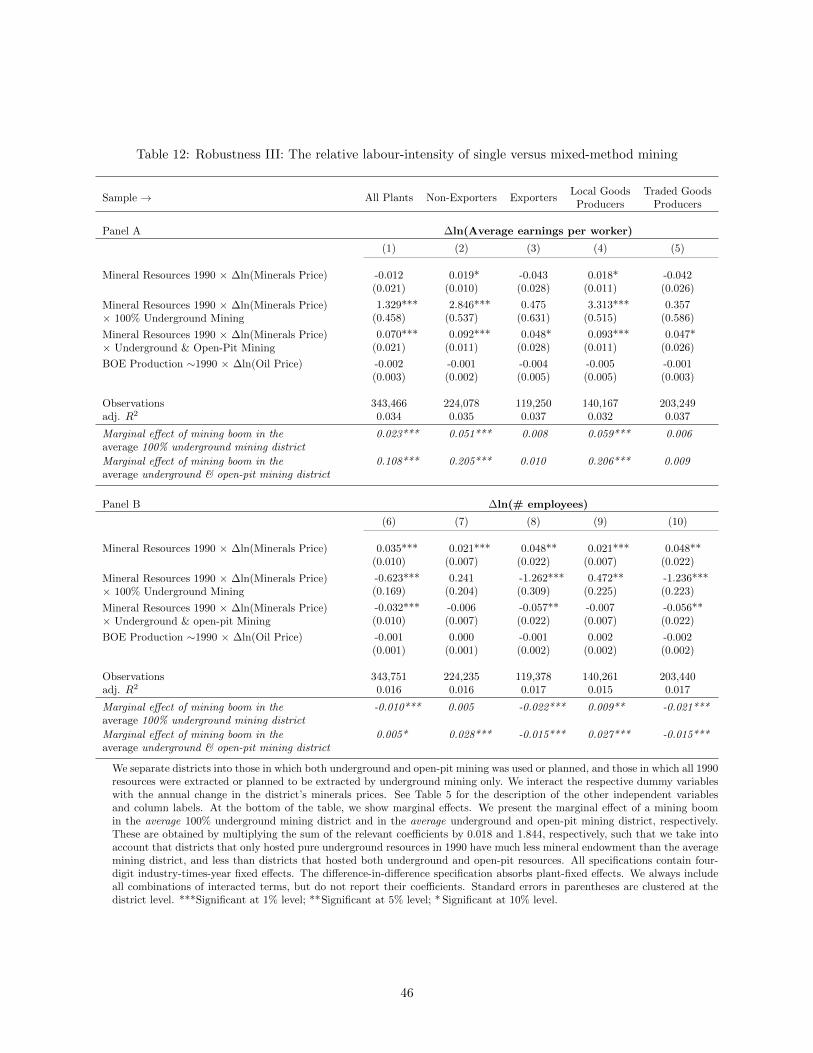
Table 12: Robustness III: The relative labour-intensity of single versus mixed-method mining

Sample → All Plants Non-Exporters ExportersLocal Goods


Producers

Panel A ∆ln(Average earnings per worker)

(1) (2) (3) (4) (5)

Mineral Resources 1990 × ∆ln(Minerals Price) -0.012 0.019* -0.043 0.018* -0.042(0.021) (0.010) (0.028) (0.011) (0.026)

Mineral Resources 1990 × ∆ln(Minerals Price)× 100% Underground Mining

1.329*** 2.846*** 0.475 3.313*** 0.357(0.458) (0.537) (0.631) (0.515) (0.586)

Mineral Resources 1990 × ∆ln(Minerals Price)× Underground & Open-Pit Mining

0.070*** 0.092*** 0.048* 0.093*** 0.047*(0.021) (0.011) (0.028) (0.011) (0.026)

BOE Production ∼1990 × ∆ln(Oil Price) -0.002 -0.001 -0.004 -0.005 -0.001(0.003) (0.002) (0.005) (0.005) (0.003)

Observations 343,466 224,078 119,250 140,167 203,249adj. R2 0.034 0.035 0.037 0.032 0.037

Marginal effect of mining boom in theaverage 100% underground mining district

0.023*** 0.051*** 0.008 0.059*** 0.006

Marginal effect of mining boom in theaverage underground & open-pit mining district

0.108*** 0.205*** 0.010 0.206*** 0.009

Panel B ∆ln(# employees)

(6) (7) (8) (9) (10)

Mineral Resources 1990 × ∆ln(Minerals Price) 0.035*** 0.021*** 0.048** 0.021*** 0.048**(0.010) (0.007) (0.022) (0.007) (0.022)

Mineral Resources 1990 × ∆ln(Minerals Price)× 100% Underground Mining

-0.623*** 0.241 -1.262*** 0.472** -1.236***(0.169) (0.204) (0.309) (0.225) (0.223)

Mineral Resources 1990 × ∆ln(Minerals Price)× Underground & open-pit Mining

-0.032*** -0.006 -0.057** -0.007 -0.056**(0.010) (0.007) (0.022) (0.007) (0.022)

BOE Production ∼1990 × ∆ln(Oil Price) -0.001 0.000 -0.001 0.002 -0.002(0.001) (0.001) (0.002) (0.002) (0.002)

Observations 343,751 224,235 119,378 140,261 203,440adj. R2 0.016 0.016 0.017 0.015 0.017

Marginal effect of mining boom in theaverage 100% underground mining district

-0.010*** 0.005 -0.022*** 0.009** -0.021***

Marginal effect of mining boom in theaverage underground & open-pit mining district

0.005* 0.028*** -0.015*** 0.027*** -0.015***

We separate districts into those in which both underground and open-pit mining was used or planned, and those in which all 1990resources were extracted or planned to be extracted by underground mining only. We interact the respective dummy variableswith the annual change in the district’s minerals prices. See Table 5 for the description of the other independent variablesand column labels. At the bottom of the table, we show marginal effects. We present the marginal effect of a mining boomin the average 100% underground mining district and in the average underground and open-pit mining district, respectively.These are obtained by multiplying the sum of the relevant coefficients by 0.018 and 1.844, respectively, such that we take intoaccount that districts that only hosted pure underground resources in 1990 have much less mineral endowment than the averagemining district, and less than districts that hosted both underground and open-pit resources. All specifications contain four-digit industry-times-year fixed effects. The difference-in-difference specification absorbs plant-fixed effects. We always includeall combinations of interacted terms, but do not report their coefficients. Standard errors in parentheses are clustered at thedistrict level. ***Significant at 1% level; **Significant at 5% level; * Significant at 10% level.

46

Online Appendix

“Good mine, bad mine: Natural resource heterogeneity and Dutch disease in Indonesia”

Paul Pelzl and Steven Poelhekke

19 July 2018

OA1 Model Proofs

Prediction 1

Proof. To see that Prediction 1, (i) and (ii) hold, use the labour market equilibrium condition (7) to rewrite

the resource sector’s profit maximization condition to prΩrF′r(L(w) − lm − ln) = w. Initially, after a rise

in pr the marginal product of labour exceeds its marginal cost. To restore equilibrium, the wage and/or

labour supply must rise. If labour supply is perfectly inelastic, i.e. L′(w) = 0, then only the wage increases.

If L′(w) > 0, then also population increases as a result of the rise in wages, since labour supply does not

rise without a wage increase, while a wage increase does trigger an increase in labour supply. Finally, for

L′(w) =∞ the wage increases by a negligible positive increment because limL′(w)→∞

∂w/∂pr = 0.

To see that Prediction 1, (iii) holds, we use the fact that resource sector profits equal prΩrFr(lr) − wlr.

Assume that resource sector employment remains constant. Further, consider first the case of perfectly

inelastic labour supply, i.e. L′(w) = 0. The non-tradable sector holds employment constant given that

resource sector employment stays constant by assumption and labour supply is unchanged. To see this, first

substitute equation (6) into equation (4) to obtain

α(w + π)L(w) = pnΩnFn(ln) (12)

Equation (8) states that pn = w/(ΩnF′n(ln)) and w = prΩrF

′r(lr). Substituting these expressions as well as

equation (2) into equation (12) and rearranging yields

Fn(ln)

F ′n(ln)= αL(w) + σα

[Fr(lr)

F ′r(lr)− lr

](13)

This equation expresses non-tradable employment as a function of resource sector employment. Taking the

first-order derivative with respect to pr yields

∂ Fn(ln)F ′n(ln)

∂pr= αL′(w)

∂w

∂pr− σα ∂lr

∂pr

Fr(lr)F′′r (lr)

[F ′r(lr)]2 (14)

Given our assumptions ∂lr/∂pr = 0 and L′(w) = 0, the right-hand side of equation (14) equals zero, which

implies ∂ln/∂pr = 0.40 We have thus shown that if labour supply is perfectly inelastic and we assume that the

40 Given that Fn(ln) is increasing in ln but concave, a change in ln increases Fn(ln) but decreases F ′n(ln), which implies

that a change in ln cannot leave Fn(ln)/F ′n(ln) unchanged. Therefore, ∂Fn(ln)F ′n(ln)

/∂pr = 0 implies ∂ln/∂pr = 0.

47

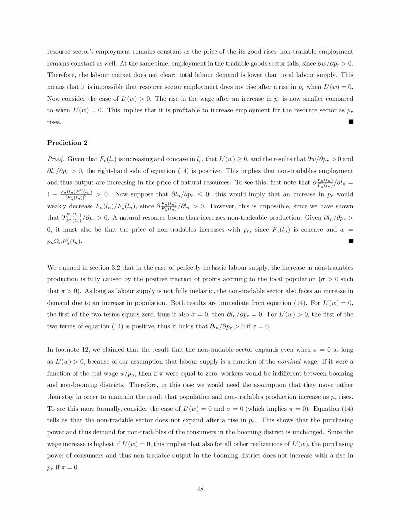
resource sector’s employment remains constant as the price of the its good rises, non-tradable employment

remains constant as well. At the same time, employment in the tradable goods sector falls, since ∂w/∂pr > 0.

Therefore, the labour market does not clear: total labour demand is lower than total labour supply. This

means that it is impossible that resource sector employment does not rise after a rise in pr when L′(w) = 0.

Now consider the case of L′(w) > 0. The rise in the wage after an increase in pr is now smaller compared

to when L′(w) = 0. This implies that it is profitable to increase employment for the resource sector as pr

rises.

Prediction 2

Proof. Given that Fr(lr) is increasing and concave in lr, that L′(w) ≥ 0, and the results that ∂w/∂pr > 0 and

∂lr/∂pr > 0, the right-hand side of equation (14) is positive. This implies that non-tradables employment

and thus output are increasing in the price of natural resources. To see this, first note that ∂ Fn(ln)F ′n(ln)

/∂ln =

1 − Fn(ln)F′′n (ln)

[F ′n(ln)]

2 > 0. Now suppose that ∂ln/∂pr ≤ 0: this would imply that an increase in pr would

weakly decrease Fn(ln)/F ′n(ln), since ∂ Fn(ln)F ′n(ln)

/∂ln > 0. However, this is impossible, since we have shown

that ∂ Fn(ln)F ′n(ln)

/∂pr > 0. A natural resource boom thus increases non-tradeable production. Given ∂ln/∂pr >

0, it must also be that the price of non-tradables increases with pr, since Fn(ln) is concave and w =

pnΩnF′n(ln).

We claimed in section 3.2 that in the case of perfectly inelastic labour supply, the increase in non-tradables

production is fully caused by the positive fraction of profits accruing to the local population (σ > 0 such

that π > 0). As long as labour supply is not fully inelastic, the non-tradable sector also faces an increase in

demand due to an increase in population. Both results are immediate from equation (14). For L′(w) = 0,

the first of the two terms equals zero, thus if also σ = 0, then ∂ln/∂pr = 0. For L′(w) > 0, the first of the

two terms of equation (14) is positive, thus it holds that ∂ln/∂pr > 0 if σ = 0.

In footnote 12, we claimed that the result that the non-tradable sector expands even when π = 0 as long

as L′(w) > 0, because of our assumption that labour supply is a function of the nominal wage. If it were a

function of the real wage w/pn, then if π were equal to zero, workers would be indifferent between booming

and non-booming districts. Therefore, in this case we would need the assumption that they move rather

than stay in order to maintain the result that population and non-tradables production increase as pr rises.

To see this more formally, consider the case of L′(w) = 0 and σ = 0 (which implies π = 0). Equation (14)

tells us that the non-tradable sector does not expand after a rise in pr. This shows that the purchasing

power and thus demand for non-tradables of the consumers in the booming district is unchanged. Since the

wage increase is highest if L′(w) = 0, this implies that also for all other realizations of L′(w), the purchasing

power of consumers and thus non-tradable output in the booming district does not increase with a rise in

pr if π = 0.

48

Prediction 3

Proof. This is immediate from the profit maximization condition of the tradable goods sector, w = pmΩmF′mk(lm):

Since pm is exogenous and ∂w/∂pr > 0, concavity of Fmk(lm) requires a reduction in employment to sat-

isfy the condition again after the rise in pr. If labour supply is perfectly elastic, the decrease in tradables

production is virtually zero since the increase in the wage is virtually zero.

Prediction 4

Proof. We start by showing that the increase in the wage is stronger the more labour-intensive the local

resource sector is, i.e. ∂(∂w∂pr

)/∂γr < 0. We first show that ∂w/∂γr < 0. To see this, assume that

∂w/∂γr = 0. We know that in equilibrium, the marginal product of labour in the resource sector equals its

marginal cost: w = prΩrF′r(lr) = prΩr

1−γrlγrr

. Taking the first order derivative of this expression with respect

to γr yields

∂[prΩr

1−γrlγrr

]∂γr

= prΩr

[-

1

lγrr+ (γ2r − γr)

1

l(γr+1)r

∂lr∂γr

](15)

Evaluated at the current level of employment, this equals -prΩr/lγrr < 0, which implies that the marginal

product of the current workforce decreases. Since we just assumed wages to remain constant, the resource

sector’s marginal cost of labour now exceeds its marginal benefit. This situation is not profit-maximizing,

thus the resource sector reduces employment.41 The tradable goods sector keeps employment constant under

constant wages. Finally, the non-tradable sector reduces employment as labour intensity of the resource sec-

tor decreases. To see this, first note that resource sector profits decrease as γr increases and the wage stays

constant.42 Further, since the wage stays constant by assumption, also labour supply stays constant. Given

that π is a positive function of resource sector profits, the left-hand side of equation (4), which is a result

of consumers’ utility maximization, is therefore now smaller than the right-hand side. Thus, for equation

(4) to hold again after the rise in γr, it must be that either pn or Cn decrease, or both. As long as only pn

decreases and Cn stays constant or rises, the non-tradables sector does not maximize profits any more, as

can be seen from equations (8) and (9). Thus, consumption of non-tradables must fall, which implies that

production and thus employment of non-tradables must fall, given equation (6). We know that in equilib-

rium, the labour market clears: ln + lm + lr = L(w). Since resource sector and non-tradables employment

decrease and tradables employment is constant, it cannot be that both the labour market clears and (4)

holds. Thus, it is impossible that ∂w/∂γr = 0. To the contrary, as γr increases, the wage must decrease to

increase labour demand and decrease labour supply (if L′(w) > 0), to restore equilibrium. We thus conclude

41 Rewrite equation (9) to lr =[prΩr(1−γr)

w

]1/γrand take the derivative with respect to γr, which yields, given our

assumption of ∂w/∂γr = 0, 1(γr−1)γ2r

[prΩr(1−γr)

w

]1/γrγr − (γr − 1) ln

[prΩr(1−γr)

w

]< 0, given that lr > 1.

42 We have just shown that if γr increases and the wage stays constant, the resource sector reduces employment. Now, if theprofits under lower employment are not lower than before the increase in γr, then it is impossible that the resource sectorwas maximizing profits prior to the increase in γr. Thus, profits fall as γr increases and the wage stays constant.

49

that ∂w/∂γr < 0.

Now take two realizations of γr: γr,low and γr,high. Since ∂w/∂γr < 0, it holds that w|γr=γr,low > w|γr=γr,high .

Suppose that ∂(∂w∂pr

)/∂γr > 0 and assume that pr rises to infinity. As long as the wage does not converge

to a finite number, this implies that in the new equilibrium, w|γr=γr,low < w|γr=γr,high . This is impossible,

since ∂w/∂γr < 0. Now, we know that the wage does not converge to a finite number as pr rises to infinity,

since in that case, equation (8) would not hold. Therefore, it must be that ∂(∂w∂pr

)/∂γr ≤ 0.

Equation (9) makes clear that the wage formation is influenced by the profit maximization problem of

the resource sector in the wake of an increase in the price of its good. The fact that the maximization

problem depends on γr implies that also the wage formation depends on γr, thus ∂(∂w∂pr

)/∂γr 6= 0. This

completes the proof that ∂(∂w∂pr

)/∂γr < 0. To gain some intuition on this result, recall that in equilibrium,

w = prΩr

[1−γrlγrr

], and thus

∂w

∂pr=

Ωr(1− γr)lγrr

[1− prγr

lr

∂lr∂pr

](16)

Now consider the two extreme cases γr = 0 and γr = 1 (which we excluded, but is possible in theory). In

the former case, ∂w/∂pr = Ωr > 0: labour is most productive, and thus as the price of the resource sector

good increases, the sector is willing to raise wages the most in order to attract additional workers. In the

latter case of γr = 1, ∂w/∂pr = 0: since the use of labour does not increase output, the resource sector

obviously does not raise wages to attract workers as the price of its good increases. In between these two

extreme cases, the larger is γr, the smaller the wage increase the resource sector optimally offers in order to

attract additional workers.

Prediction 4, (ii) follows immediately from ∂(∂w∂pr

)/∂γr < 0. As long as labour supply is not perfectly

inelastic, i.e. as long as L′(w) > 0, a larger wage increase following a rise in pr when γr is lower implies a

larger increase in population.

To prove Prediction 4, (iii), we first write out non-tradable employment explicitly by substituting the pro-

duction functions and its first derivatives with respect to labour, respectively, into equation (13):

ln = α(1− γn)

[L(w) + σ

(lr

1− γr− lr

)](17)

We then derive ∂ln/∂pr:

∂ln∂pr

= α(1− γn)

[L′(w)

∂w

∂pr+ σ

∂lr∂pr

(1

1− γr− 1

)](18)

Taking the derivative of this expression with respect to γr yields

50

∂(∂ln∂pr

)∂γr

= α(1− γn)

L′(w)∂(∂w∂pr

)∂γr

+ σ

∂(∂lr∂pr

)∂γr

(1

1− γr− 1

)+∂lr∂pr

1

(1− γr)2

(19)

We now evaluate the sign of ∂(∂ln∂pr

)/∂γr under all possible realizations of L′(w). Let us define

−σ

[∂( ∂lr∂pr

)∂γr

(1

1−γr − 1)

+ ∂lr∂pr

1(1−γr)2

][∂( ∂w∂pr )∂γr

] ≡ B (20)

Now the following relationships hold:

L′(w) > B →∂(∂ln∂pr

)∂γr

< 0 ; L′(w) = B →∂(∂ln∂pr

)∂γr

= 0 ; L′(w) < B →∂(∂ln∂pr

)∂γr

> 0

To get some intuition on these results, consider the two extreme cases of labour supply elasticity. In the

case of L′(w) = ∞, it is clear from expression (19) that ∂(∂ln∂pr

)/∂γr < 0, since ∂

(∂w∂pr

)/∂γr < 0. In-

tuitively, conditional on a given labour intensity of its production process, the resource sector increases

employment most after a given rise in the price of its good when L′(w) =∞. It is then cheapest to attract

additional workers and raise employment. All newly-hired employees immigrate from other districts, thus

the non-tradable sector faces no competition for labour from the resource sector as the latter expands. At

the same time, each immigrant into the booming district increases aggregate demand for the non-tradable

sector. Thus, the larger the increase of the resource sector’s labour demand, the larger the expansion of

the non-tradable sector. Now, since an increase in the resource sector’s labour intensity increases its rise in

demand for labour as the price of its good increases (see Prediction 4, (iv)), it is intuitive that for L′(w) =∞,

∂(∂ln∂pr

)/∂γr < 0.

Now consider the other extreme case of labour supply elasticity, L′(w) = 0, and assume that γr = 0. In

this scenario, labour is most productive in the production of the resource sector good and immobile across

districts. For these reasons, the non-tradable sector faces sharp competition for additional labour from the

resource sector. Thus, there is little scope for the non-tradable sector to raise employment as pr increases.

Now suppose that γr is larger, and equal to 1− ε, where ε is a positive but infinitesimally small number. In

this case, the resource sector employs virtually no labour, and thus its partial-equilibrium wage response to

an increase in pr is virtually zero. At the same time, resource sector profits increase – as always when pr

rises –, and consumers participate in this rise in profits, which increases their purchasing power. Since the

wage the resource sector offers is virtually unchanged, this implies that there is considerable scope for the

non-tradable sector to raise wages and production, until a new equilibrium is reached. This illustrates that

in our example of L′(w) = 0 and γr = 0, ∂(∂ln∂pr

)/∂γr > 0, as can be seen from equation (19).

51

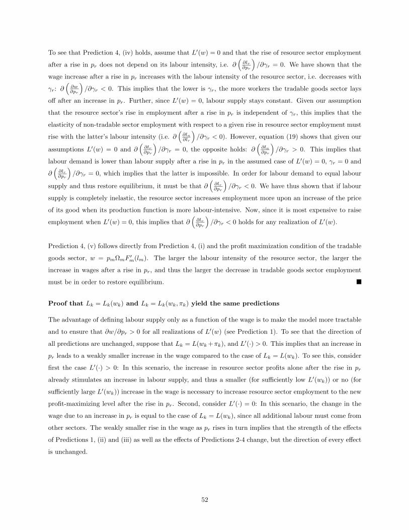
To see that Prediction 4, (iv) holds, assume that L′(w) = 0 and that the rise of resource sector employment

after a rise in pr does not depend on its labour intensity, i.e. ∂(∂lr∂pr

)/∂γr = 0. We have shown that the

wage increase after a rise in pr increases with the labour intensity of the resource sector, i.e. decreases with

γr: ∂(∂w∂pr

)/∂γr < 0. This implies that the lower is γr, the more workers the tradable goods sector lays

off after an increase in pr. Further, since L′(w) = 0, labour supply stays constant. Given our assumption

that the resource sector’s rise in employment after a rise in pr is independent of γr, this implies that the

elasticity of non-tradable sector employment with respect to a given rise in resource sector employment must

rise with the latter’s labour intensity (i.e. ∂(∂ln∂lr

)/∂γr < 0). However, equation (19) shows that given our

assumptions L′(w) = 0 and ∂(∂lr∂pr

)/∂γr = 0, the opposite holds: ∂

(∂ln∂pr

)/∂γr > 0. This implies that

labour demand is lower than labour supply after a rise in pr in the assumed case of L′(w) = 0, γr = 0 and

∂(∂lr∂pr

)/∂γr = 0, which implies that the latter is impossible. In order for labour demand to equal labour

supply and thus restore equilibrium, it must be that ∂(∂lr∂pr

)/∂γr < 0. We have thus shown that if labour

supply is completely inelastic, the resource sector increases employment more upon an increase of the price

of its good when its production function is more labour-intensive. Now, since it is most expensive to raise

employment when L′(w) = 0, this implies that ∂(∂lr∂pr

)/∂γr < 0 holds for any realization of L′(w).

Prediction 4, (v) follows directly from Prediction 4, (i) and the profit maximization condition of the tradable

goods sector, w = pmΩmF′m(lm). The larger the labour intensity of the resource sector, the larger the

increase in wages after a rise in pr, and thus the larger the decrease in tradable goods sector employment

must be in order to restore equilibrium.

Proof that Lk = Lk(wk) and Lk = Lk(wk, πk) yield the same predictions

The advantage of defining labour supply only as a function of the wage is to make the model more tractable

and to ensure that ∂w/∂pr > 0 for all realizations of L′(w) (see Prediction 1). To see that the direction of

all predictions are unchanged, suppose that Lk = L(wk+πk), and L′(·) > 0. This implies that an increase in

pr leads to a weakly smaller increase in the wage compared to the case of Lk = L(wk). To see this, consider

first the case L′(·) > 0: In this scenario, the increase in resource sector profits alone after the rise in pr

already stimulates an increase in labour supply, and thus a smaller (for sufficiently low L′(wk)) or no (for

sufficiently large L′(wk)) increase in the wage is necessary to increase resource sector employment to the new

profit-maximizing level after the rise in pr. Second, consider L′(·) = 0: In this scenario, the change in the

wage due to an increase in pr is equal to the case of Lk = L(wk), since all additional labour must come from

other sectors. The weakly smaller rise in the wage as pr rises in turn implies that the strength of the effects

of Predictions 1, (ii) and (iii) as well as the effects of Predictions 2-4 change, but the direction of every effect

is unchanged.

52

OA2 Mining Data

Combining RMD and MinEx data

The data sources we use to compute district-specific mineral resources as of 1990 are Raw Materials Data

(RMD in the following) and MinEx Consulting (MinEx in the following). Both datasets claim full coverage,

and indeed, the majority of deposits listed in one dataset are also reported in the other. We also double-

checked the reported deposits with public data from the USGS Mineral Resources Data System (MRDS)

(which lists less deposits than RMD and MinEx ). We match deposits across the data sources using the name

of the deposits. For all remaining deposits, we carefully check if a deposit in a given dataset corresponds

to a deposit in the other dataset, using additional variables such as deposit location and ore resources. If

a deposit remains unmatched after this procedure, we nonetheless included it into our sample. In total, we

identify 82 mineral deposits which had positive mineral resources in 1990. 49 of these deposits are listed

in both datasets, while the remaining 33 are only listed in one source. These 33 deposits have statistically

significantly lower mineral resources as of 1990 compared to those listed in both datasets. 24 of the 33

deposits are unique to MinEx and nine are unique to RMD. For matched deposits for which information

is available in both datasets for a specific variable, we use the MinEx data (see below for variable-specific

details). We are more confident about the accuracy of the MinEx data because a test in Google Earth reveals

that the MinEx location data is more precise compared to RMD.

Location of resources

Both RMD and MinEx report the location of a deposit in terms of latitude and longitude. For the set of

deposits that were operated by a mine over our sample period and for which different latitude and longitude

data is reported by MinEx and RMD, we entered the location data into Google Earth and regard the location

displaying a mine as the correct one. Since the MinEx data proves more accurate among these deposits, we

also choose to use the MinEx data when in neither of the locations we saw a mine (which can be due to a

mine no longer being operated). For three deposits, our data sources do not provide data on the location;

we retrieved these via Internet search (sources available on request). With the chosen latitude and longitude

data at hand, we first identify the home district of the deposit as of 2016, using Google Maps. In a second

step, we assign the district to its 1990-district, if the two differ, using district proliferation tables provided

by Indonesia’s national statistical agency, Badan Pusat Statistik (BPS), and information provided by Bazzi

and Gudgeon (2018).

Time of discovery of resources

Only MinEx reports the year of discovery. It is missing for around one third of deposits. Since we are only

interested whether discovery took place before 1990, for several of these deposits we can answer this question

53

due to the fact that production started before 1990. For all remaining deposits, we attempted to find out

if discovery was prior to 1990 via Internet search. We achieved this for 42 deposits, mostly using company

yearbooks or mining information websites.43 Further, we infer that the discovery, if at all, took place after

1990 if in 2016 (the year in which we obtained the then up-to-date MinEx data), the deposit’s status is

either “Advanced Exploration”, “Emerging Project” or different subgroups containing the term “Feasibility

Study”. For all deposits that are only listed in the RMD dataset, we also use the pre-1990 production

start-up rule, Internet search (23 deposits) and the deposit’s status to infer the discovery date, in this order.

Concerning deposit status, we infer that the discovery, if at all, took place after the most recent year for

which the deposit’s status is either “Project, no specification”, “Conceptual”, “Feasibility”, “Prefeasibility”,

“Abandoned Project” or “Abandoned”. For the remaining deposits from both datasets with missing dis-

covery date, we infer it as the year of production start-up minus the median difference between discovery

year and production start-up year across all mines for which we have information on both, which is 8 years.44

Multi-mineral deposits

For a given deposit, RMD reports annual production figures per extracted mineral. This implies that we

know about the existence of a specific mineral in a given deposit only if the mineral was extracted in any

year over the period the RMD data covers, which is 1975-2011. 11 deposits in our final sample (thus with

positive 1990 ore resources) that are listed in RMD produced more than one mineral at any point in time

between 1975 and 2011. These 11 deposits are spread across 11 districts. Unfortunately, we do not know the

share of each mineral in total ore resources for the 11 deposits. We thus infer the share of mineral m in total

resources using the average ratio of ore production of mineral m over total ore production of the respective

deposit, using all years in which the deposit was operated and production data is available. Since production

is reported in terms of metal, not ore, we convert metal to ore using the reported mineral-specific grades

of each deposit. If the latter is not reported, we infer it by computing the average grade of the respective

mineral using the available information among all deposits containing that mineral. In the 11 districts that

hosted at least one multi-mineral deposit, we incorporate the inferred shares of respective minerals in multi-

mineral deposits into our computation of the “general mineral price level” of the district.

MinEx only lists the main mineral of a given deposit. Therefore, inferring mineral-specific resources for a

given deposit is not possible for those that were potentially hosting multiple minerals but were only listed in

MinEx. For all these deposits, we are forced to assume that the main mineral is in fact the only contained

mineral. Given the low percentage of multi-mineral deposits in RMD and the fact that deposits only listed

in MinEx have low ore resources, we do not expect this to affect our results.

43 For some deposits, we proxy discovery with the year of establishment of the company (or branch) which operated thedeposit, if the name of the company or branch contains the name of the deposit. Since for all these deposits that year wasafter 1990 this turned out to be equivalent to dropping the deposits from our sample.

44 We drop one single (small) deposit from our sample for which neither the discovery year nor production start-up year isreported.

54

Inferring missing ore resources data

Ore resource data is missing for a number of deposits in our dataset. Whenever this is the case but ore

reserves data is non-missing, we infer ore resources as ore reserves times the mineral-specific average ratio

of resources and reserves in our dataset.45 In case there is no other deposit of the same mineral with non-

missing resources and reserves data, we infer resources as reserves times the average ratio of resources and

reserves across all deposits and minerals. If both reserves and resource data are missing, we retrieve resources

or reserves data using Internet research. There are no deposits that were discovered before 1990 for which

we were unable to retrieve resources or reserves data.

Ore reserves and resource data is missing for all tin deposits in both RMD and MinEx. Therefore, we

retrieve the missing data via Internet search. Since we could not obtain deposit-specific resources data, we

use resources data of public operator PT Timah, which has a monopoly on tin mining in Indonesia. Total

tin resources of PT Timah, and thus Indonesia, amounted to 1.06 Million tons of tin as of 2008, according

to the annual report of PT Timah of that year. We were unable to retrieve ore reserves data for an earlier

year. In order to infer tin resources as of 1990, we add total tin production over 1990-2008 to the 2008 figure,

using annual production data from Indonesia’s Department of Mines and Energy, which is made available

by the U.S. Bureau of Mines. Since RMD and MinEx do not contain any grade information for Indonesian

tin deposits, we convert the resulting number to tons of ore rather than tons of tin using the average ratio

provided by different sources. Specifically, according to earthsci.org, “Indonesia produces tin mainly from

alluvial deposits” (http : //earthsci.org/mineral/mindep/depfile/tin.htm), and the ratio of ore and tin

from alluvial deposits ranges between 0.01 and 0.015 per cent across different sources; we thus infer a ratio of

0.0125 for our analysis. Since PT Timah annual reports do not indicate the distribution of resources across

Indonesia’s tin deposits, we infer the shares using mine-specific annual production data from Indonesia’s

Department of Mines and Energy. While data on annual aggregate tin production in Indonesia is available

from 1949-2008, mine-specific production data is only available for the period 1978-1988 (see Wu, 1982-

1989), thus we compute the production shares using the data from this period. Since we cannot attribute tin

deposits in these data in the districts Bangka and Belitung to either of the two districts, we treat these two

1990-districts as one district in our analysis. Approximately 91% of Indonesian tin production took place in

mines located in the Bangka-Belitung archipelago on average over 1978-1988. We thus infer the tin reserves

of Bangka-Belitung as this percentage times our measure of total tin reserves as of 1990. The remaining

9% of tin production over 1978-1988 took place in mines in the Riau archipelago; we thus inferred 1990 tin

resources of the 1990-district Riau using the same method.

45 These ratios are obtained from RMD, since MinEx only reports ore resources. Resources are “the concentration oroccurrence of material of intrinsic economic interest in or on the Earth’s crust in such form and quantity that there arereasonable prospects for eventual economic extraction” (Raw Materials Data Handbook, p.57). Reserves are defined as“the economically mineable part of a measured or indicated mineral resource” (p.58).

55

Computation of district-specific 1990 ore resources

We first compute mineral ore resources as of 1990 for each deposit. We then sum 1990 resources across all

deposits in a district and divide the result by the district size in square miles.

If a deposit was discovered before 1990 but did not start production before that year, the deposit’s 1990

resources simply equal its initial resources. If a deposit was operated by a mine before 1990, we deduct the

mine’s pre-1990 ore production from the initial resources to arrive at the deposit-specific ore resources as of

1990. For all deposits contained in RMD, this is done using annual production data. For all deposits unique

to MinEx, annual production data is not reported, thus we infer total production before 1990 as average

annual production times the number of production years before 1990.46 In the RMD data, in some cases,

pre-1990 production of a mine is only reported in terms of metal, rather than ore. In this case, we compute

the average ratio of ore and metal production of the specific mine and metal for each year in which both are

available, and use this ratio to infer ore production in a given pre-1990 year in which it is missing. If ore

production is not available for any year, then we instead use the mine- and metal-specific grade to infer ore

production from metal production. If the grade is not reported by our data sources, we tried to retrieve it

via Internet search. If this search was unsuccessful, we infer ore production using the average grade of the

same metal (i) in the same district, (ii) in the same province or (iii) in Indonesia overall – in this order, based

on the distribution of metals across space and data availability. For five mines which started production

before 1990 and which are reported in RMD, pre-1990 production data is entirely unavailable. In these cases,

we infer pre-1990 production as the average yearly (post-1990) production across years in which production

data is reported in RMD, multiplied by the number of pre-1990 production years. In one case, we do not

have any information on production; in this case, we infer 1990 ore resources as initial resources.

OA3 Oil and Gas data

The Indonesia, Oil and Gas Atlas is divided into six volumes, each of which covers a certain geographical

area. Specifically, these are North Sumatra and Natuna (Volume 1, 1989), Central Sumatra (Volume 2,

1991), South Sumatra (Volume 3, 1990), Java (Volume 4, 1989), Kalimantan (Volume 5, 1991) and Eastern

Indonesia (Volume 6, 1988). We assign a field producing oil and/or gas to its respective 1990 district by

first identifying the 2017-district in which the field is located, using data on the field’s latitude and longitude

provided in the data source. We then identify the corresponding 1990 district using district proliferation

tables (see Online Appendix OA2). If a field is located offshore, we assign it to the closest district in terms

of geographical distance.

46 MinEx reports both “initial resources”, the year of production commencement and “current resources”. The moment intime in which the latter is reported varies by mine. We compute annual average production as the difference betweeninitial resources and current resources, divided by the number of years between production commencement and the yearin which current resources are reported.

56

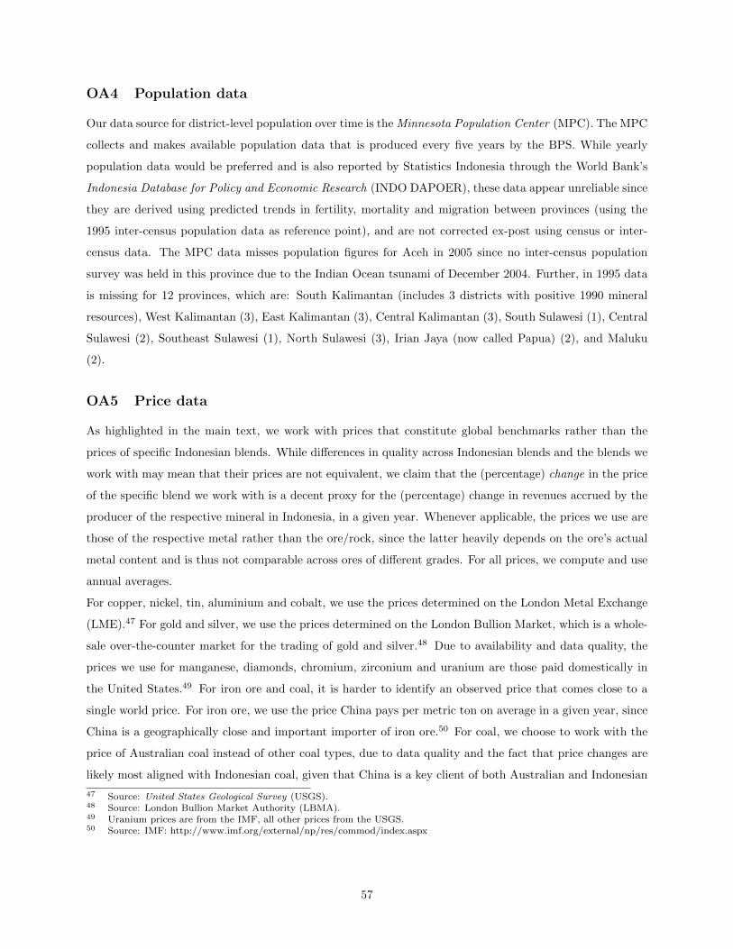
OA4 Population data

Our data source for district-level population over time is the Minnesota Population Center (MPC). The MPC

collects and makes available population data that is produced every five years by the BPS. While yearly

population data would be preferred and is also reported by Statistics Indonesia through the World Bank’s

Indonesia Database for Policy and Economic Research (INDO DAPOER), these data appear unreliable since

they are derived using predicted trends in fertility, mortality and migration between provinces (using the

1995 inter-census population data as reference point), and are not corrected ex-post using census or inter-

census data. The MPC data misses population figures for Aceh in 2005 since no inter-census population

survey was held in this province due to the Indian Ocean tsunami of December 2004. Further, in 1995 data

is missing for 12 provinces, which are: South Kalimantan (includes 3 districts with positive 1990 mineral

resources), West Kalimantan (3), East Kalimantan (3), Central Kalimantan (3), South Sulawesi (1), Central

Sulawesi (2), Southeast Sulawesi (1), North Sulawesi (3), Irian Jaya (now called Papua) (2), and Maluku

(2).

OA5 Price data

As highlighted in the main text, we work with prices that constitute global benchmarks rather than the

prices of specific Indonesian blends. While differences in quality across Indonesian blends and the blends we

work with may mean that their prices are not equivalent, we claim that the (percentage) change in the price

of the specific blend we work with is a decent proxy for the (percentage) change in revenues accrued by the

producer of the respective mineral in Indonesia, in a given year. Whenever applicable, the prices we use are

those of the respective metal rather than the ore/rock, since the latter heavily depends on the ore’s actual

metal content and is thus not comparable across ores of different grades. For all prices, we compute and use

annual averages.

For copper, nickel, tin, aluminium and cobalt, we use the prices determined on the London Metal Exchange

(LME).47 For gold and silver, we use the prices determined on the London Bullion Market, which is a whole-

sale over-the-counter market for the trading of gold and silver.48 Due to availability and data quality, the

prices we use for manganese, diamonds, chromium, zirconium and uranium are those paid domestically in

the United States.49 For iron ore and coal, it is harder to identify an observed price that comes close to a

single world price. For iron ore, we use the price China pays per metric ton on average in a given year, since

China is a geographically close and important importer of iron ore.50 For coal, we choose to work with the

price of Australian coal instead of other coal types, due to data quality and the fact that price changes are

likely most aligned with Indonesian coal, given that China is a key client of both Australian and Indonesian

47 Source: United States Geological Survey (USGS).48 Source: London Bullion Market Authority (LBMA).49 Uranium prices are from the IMF, all other prices from the USGS.50 Source: IMF: http://www.imf.org/external/np/res/commod/index.aspx

57

coal.51 For crude oil, we use the price of West Texas Intermediate (WTI), which is a benchmark for the prices

of other crude oil sorts.52 We do not account for natural gas prices separately, both in order to follow the

tradition of the literature and because natural gas prices are in any case highly correlated with crude oil prices.

OA6 Manufacturing Census Data

Cleaning

We drop plant-years in which production worker employment is larger than total employment, as well as

plant-years in which the reported number of employees is below 20.53 Further, we drop six plants that have

a district ID that does not correspond to any district ID we observe in our BPS list of district IDs. Around

6% of plants are reported to operate in different (mostly two) 1990-districts in different years. This could

be caused by changes in district borders that are not explained by district splits or, more likely, by plants

moving from one 1990-district to another during our sample period. Importantly, the plant fixed effects that

we control for by first-differencing our outcome variables at the plant level only nest district-specific fixed

effects if plants in our sample do not change 1990-district. We therefore keep the plant’s district-years of the

1990-district it stayed in for the longest time period over 1990-2009, and drop the plant’s other district-year

observations.

Defining local versus traded goods producers

For each of the 473 six-digit industries of the 1997 North American Industry Classification System (NAICS

1997), Holmes and Stevens (2014) estimate a (constant) distance elasticity, which equals the percentage

change in trade volume as distance increases by one percent. They do so using the 1997 U.S. Commodity

Flow Survey (CFS) data, which documents the destination, product classification, weight and value of a broad

sample of shipments that leave manufacturing plants. Holmes and Stevens (2014) estimate an industry’s

constant distance elasticity via a standard log-log specification typically used in the trade literature. This

specification has distance adjustment, which increases with industry-specific trade costs, on the left-hand

side and distance on the right-hand side. Intuitively, the higher the trade costs of a specific industry, the

shorter its optimal average shipment distance (equivalently, the higher its distance adjustment). Ready-

Mix Concrete (4.2), Ice (3.0) and Asphalt (2.9) have the highest estimated distance elasticity. In turn, 29

industries have an estimated distance elasticity of zero, including Semiconductors, Analytical laboratory

instruments and Aircraft, in which transportation costs are very low relative to product value.

We use the estimates of Holmes and Stevens to classify plants into local and traded goods producers. Our

51 Source: IMF: http://www.imf.org/external/np/res/commod/index.aspx52 Source: Energy Information Administration (EIA)53 The fact that only few plants had less than 20 employees made clear to us that indeed, if a plant that had been registered

the year before went below the threshold of 20 employees, it was not registered in the following year. We conclude thatrealizations of employees below 20 must be typos.

58

plant-level data contains information on the 4-digit sector of each plant. The industry classification system

is the 2000 version of the Klasifikasi Baku Lapangan Usaha (KBLI 2000). This roughly corresponds to

Revision 3.1. of the International Standard Industry Classification (ISIC Rev. 3.1), however not one-to-one.

Therefore, we first use KBLI 2000 and ISIC Rev.3.1 documentation files to determine the equivalent, or

closest in nature, ISIC Rev.3.1 code of all KBLI 2000 codes. Next, we walk from ISIC Rev. 3.1 to NAICS

1997 using concordance tables provided by the United States Census Bureau. Since our sample contains 123

(ISIC Rev. 3.1) industries, in the great majority of cases, one four-digit ISIC Rev.3.1 industry code matches

with more than one NAICS 1997 code. In all these cases, we compute the ISIC-realization of the distance

elasticity as the average realization across all the NAICS industries matching with the particular ISIC code.

Defining upstream plants

The 2007 input-output tables of the Bureau of Economic Analysis (BEA) distinguish three mining industries

that, taken together, we refer to as the “the mining sector” : 1. “Coal mining”; 2. “Iron, gold, silver and

other metal ore mining”; and 3. “Copper, nickel, lead and zinc mining”. Details on the concordance of the

ISIC Rev.3.1 codes used in the manufacturing census and the BEA codes used in the input-output tables are

described further below. For each of the 389 industries j that are distinguished in the 2007 Input-Output

tables of the BEA, we compute its ‘upstreamness’ to the mining sector as the ratio of the (weighted) sum of

its direct and indirect sales to the mining sector (as defined above) and its total sales:

Upstreamjk =

∑m Salesj,m × (Rkm/Rk)∑

j Salesj+∑−J

[Salesj,−j∑j Salesj

∗∑m Sales−j,m × (Rkm/Rk)∑

j Sales−j,j

]∈ [0, 1] (21)

where −J denotes the set of all industries apart from j, k is the district identifier as usual and

m=Coal mining; Iron, gold, silver and other metal ore mining; Copper, nickel, lead and zinc mining. Rkmequals the total 1990 resources of the minerals contained in group m in district k and Rk the total 1990

mineral resources in district k. The chosen upstream measure thus takes into account which minerals are

locally produced, which makes it industry- and district-specific rather than only industry-specific. Therefore,

if for example industry j is only upstream to the coal mining sector and there are no coal deposits but only

gold deposits as of 1990 in district k, then we don’t classify plants in industry j in district k as upstream,

such that Upstreamjk = 0. The reasoning behind this choice is that in our empirical analysis, we try to test

whether any effect of a local mining boom is driven by plants that are upstream to the local mining sector.

Using our previous example, we do not expect plants that sell to the coal sector to benefit or suffer more

from a gold boom in their home district than plants in the same district that do not sell to any of the three

mining sectors, since neither group of plants sells to the sector Iron, gold, silver and other metal ore mining.

On the other hand, if coal deposits were present in district k, then the plants selling to the coal sector might

perform differently, and the more important the coal mining sector is in district k, the more so.

59

The industries in the BEA input-output tables are classified using BEA codes. We first walk from the BEA

codes to the 2002 NAICS codes, and then match those with the ISIC Rev.3.1 codes, using concordance tables

provided by the United States Census Bureau. The census data reports 133 distinct four-digit ISIC Rev.

3.1 manufacturing industries, while the BEA tables feature 389 industries. As a consequence, in the great

majority of cases, one four-digit ISIC industry code matches with more than one BEA code. In all these cases,

we compute the realization of Upstreamjk as the average realization across all the BEA industries matching

with the particular ISIC code. We argue that the inferred value provides a reasonable approximation, since

the realizations of Upstreamjk are very similar across BEA codes that match with the same ISIC code.

OA7 SAKERNAS Data

While the household survey SAKERNAS was initiated in 1976, only from 2007 onwards, the survey data

has been representative at the district level. In any given year after 2006, only the August round is rep-

resentative at the district level, which is why we use data from those rounds. SAKERNAS has covered all

1990-districts in the August rounds in 2007-2015 except the years 2013 (five districts missing) and 2015 (one

district missing) and includes data on between 490,468 (in 2014) and 953,172 (in 2010) individuals.54 This

implies a coverage of between 0.2 and 0.4 percent.

We use SAKERNAS to approximate the number of workers employed in the mining or oil and gas sector (see

Table 3) and the number of workers employed in the mining sector (see Table OA1) in a given district and

year, from 2007-2015. To compute the prior, we first compute the weighted share of surveyed individuals

who reported to work in the mining or oil and gas sector, in a given district-year. The numerator of this

share is the weighted number of respondents in the district-year who state that their main activity in the past

week was working and who report to work in one of the following sectors: Coal Mining and Peat Excavation,

Uranium and Thorium Mining, Metal Mining, Oil and Gas. The denominator is the weighted number of

respondents in the district-year. We use the sample weight attached to each individual respondent in the

data. We multiply the computed share by the district population according to the most recent available

population census or inter-census population survey, from the specific year’s perspective, and take the log of

the result.55 To approximate the number of mining workers, we repeat the above exercise, but exclude oil

and gas workers from the numerator of the share.

As a descriptive statistic, in Table 2 we also report the average district-year specific fraction of mining and

oil and gas workers to total workers and the fraction of mining workers to total workers, over 2007-2015.

For a given district and year, the numerators of these shares are equivalent to the numerators just described

54 In a given district, certain census blocks are selected, in which 16 households are sampled (10 from 2011 onwards). Allindividuals sampled in a certain census block obtain the same weight, which depends on the relative importance of thecensus block in terms of overall district representation.

55 We multiply the share of mining workers in 2015 with the population data from 2010, since the results of the 2015inter-census population survey have not been published by the MPC yet.

60

above. The denominator of both shares is the weighted number of surveyed individuals who state that their

main activity in the past week was working.

61

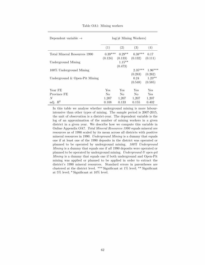
Table OA1: Mining workers

Dependent variable → log(# Mining Workers)

(1) (2) (3) (4)

Total Mineral Resources 1990 0.39*** 0.29** 0.38*** 0.17(0.124) (0.133) (0.132) (0.111)

Underground Mining 1.15**(0.473)

100% Underground Mining 2.35*** 1.96***(0.283) (0.262)

Underground & Open-Pit Mining 0.24 1.23**(0.548) (0.585)

Year FE Yes Yes Yes YesProvince FE No No No YesN 1,207 1,207 1,207 1,207adj. R2 0.108 0.133 0.155 0.402

In this table we analyse whether underground mining is more labour-intensive than other types of mining. The sample period is 2007-2015,the unit of observation is a district-year. The dependent variable is thelog of an approximation of the number of mining workers in a givendistrict in a given year. We describe how we compute this variable inOnline Appendix OA7. Total Mineral Resources 1990 equals mineral oreresources as of 1990 scaled by its mean across all districts with positivemineral resources in 1990. Underground Mining is a dummy that equalsone if at least one of the 1990 deposits in the district was operated orplanned to be operated by underground mining. 100% UndergroundMining is a dummy that equals one if all 1990 deposits were operated orplanned to be operated by underground mining. Underground & open-pitMining is a dummy that equals one if both underground and Open-Pitmining was applied or planned to be applied in order to extract thedistrict’s 1990 mineral resources. Standard errors in parentheses areclustered at the district level. *** Significant at 1% level; ** Significantat 5% level; * Significant at 10% level.

62

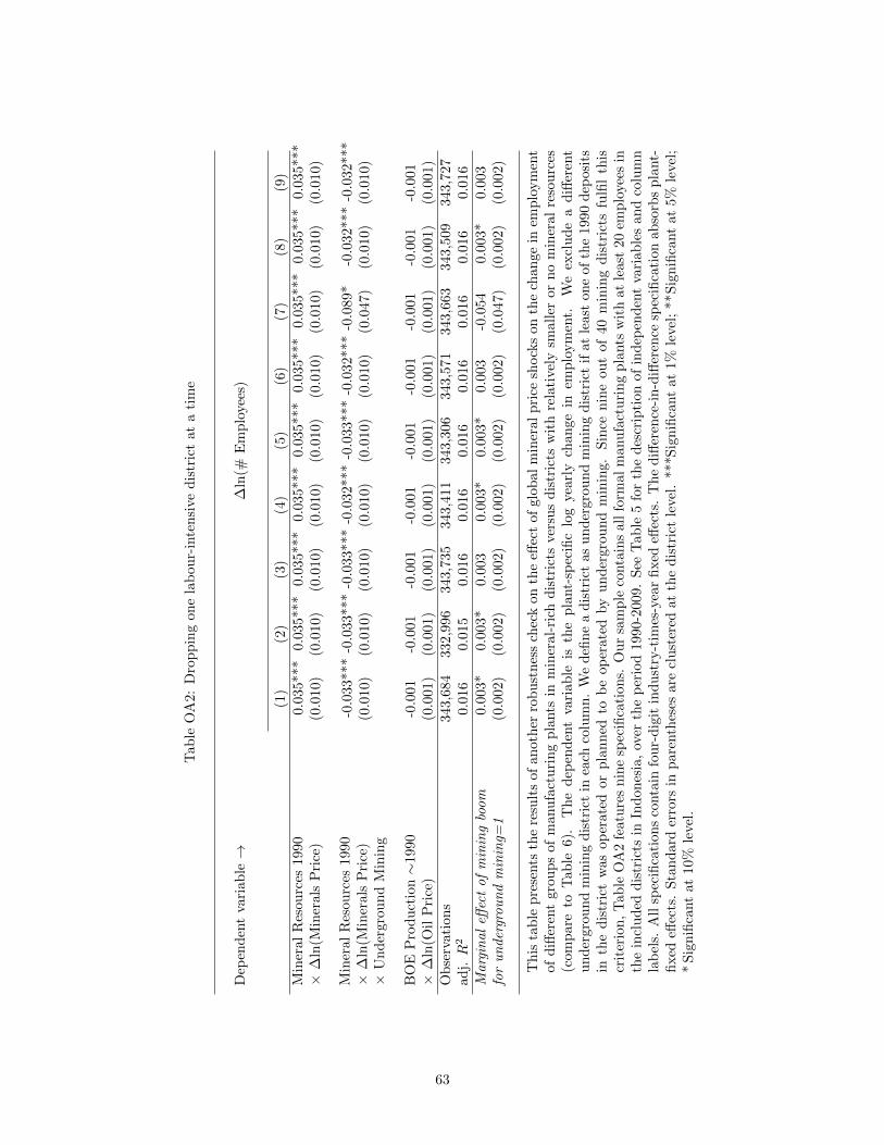
Tab

leO

A2:

Dro

pp

ing

on

ela

bou

r-in

ten

sive

dis

tric

tat

ati

me

Dep

end

ent

vari

able→

∆ln

(#E

mp

loyee

s)

(1)

(2)

(3)

(4)

(5)

(6)

(7)

(8)

(9)

Min

eral

Res

ourc

es19

90×

∆ln

(Min

eral

sP

rice

)0.0

35***

0.0

35***

0.0

35***

0.0

35***

0.0

35***

0.0

35***

0.0

35***

0.0

35***

0.0

35***

(0.0

10)

(0.0

10)

(0.0

10)

(0.0

10)

(0.0

10)

(0.0

10)

(0.0

10)

(0.0

10)

(0.0

10)

Min

eral

Res

ourc

es19

90×

∆ln

(Min

eral

sP

rice

)×

Un

der

grou

nd

Min

ing

-0.0

33***

-0.0

33***

-0.0

33***

-0.0

32***

-0.0

33***

-0.0

32***

-0.0

89*

-0.0

32***

-0.0

32***

(0.0

10)

(0.0

10)

(0.0

10)

(0.0

10)

(0.0

10)

(0.0

10)

(0.0

47)

(0.0

10)

(0.0

10)

BO

EP

rod

uct

ion∼

1990

×∆

ln(O

ilP

rice

)-0

.001

-0.0

01

-0.0

01

-0.0

01

-0.0

01

-0.0

01

-0.0

01

-0.0

01

-0.0

01

(0.0

01)

(0.0

01)

(0.0

01)

(0.0

01)

(0.0

01)

(0.0

01)

(0.0

01)

(0.0

01)

(0.0

01)

Ob

serv

atio

ns

343,6

84

332,9

96

343,7

35

343,4

11

343,3

06

343,5

71

343,6

63

343,5

09

343,7

27

adj.R

20.0

16

0.0

15

0.0

16

0.0

16

0.0

16

0.0

16

0.0

16

0.0

16

0.0

16

Marg

inal

effec

tof

min

ing

boom

for

un

der

grou

nd

min

ing=

10.0

03*

0.0

03*

0.0

03

0.0

03*

0.0

03*

0.0

03

-0.0

54

0.0

03*

0.0

03

(0.0

02)

(0.0

02)

(0.0

02)

(0.0

02)

(0.0

02)

(0.0

02)

(0.0

47)

(0.0

02)

(0.0

02)

Th

ista

ble

pre

sents

the

resu

lts

ofan

oth

erro

bust

nes

sch

eck

on

the

effec

tof

glo

bal

min

eral

pri

cesh

ock

son

the

chan

ge

inem

plo

ym

ent

ofd

iffer

ent

grou

ps

ofm

anu

fact

uri

ng

pla

nts

inm

iner

al-

rich

dis

tric

tsve

rsu

sd

istr

icts

wit

hre

lati

vely

small

eror

no

min

eral

reso

urc

es(c

omp

are

toT

able

6).

Th

ed

epen

den

tva

riab

leis

the

pla

nt-

spec

ific

log

yea

rly

chan

ge

inem

plo

ym

ent.

We

excl

ud

ea

diff

eren

tu

nd

ergr

oun

dm

inin

gd

istr

ict

inea

chco

lum

n.

We

defi

ne

ad

istr

ict

as

un

der

gro

un

dm

inin

gd

istr

ict

ifat

least

on

eof

the

1990

dep

osi

tsin

the

dis

tric

tw

asop

erat

edor

pla

nn

edto

be

op

erate

dby

un

der

gro

un

dm

inin

g.

Sin

cen

ine

ou

tof

40

min

ing

dis

tric

tsfu

lfil

this

crit

erio

n,

Tab

leO

A2

feat

ure

sn

ine

spec

ifica

tion

s.O

ur

sam

ple

conta

ins

all

form

al

manu

fact

uri

ng

pla

nts

wit

hat

least

20

emp

loye

esin

the

incl

ud

edd

istr

icts

inIn

don

esia

,ov

erth

ep

erio

d1990-2

009.

See

Tab

le5

for

the

des

crip

tion

of

ind

epen

den

tva

riab

les

an

dco

lum

nla

bel

s.A

llsp

ecifi

cati

ons

conta

info

ur-

dig

itin

du

stry

-tim

es-y

ear

fixed

effec

ts.

Th

ediff

eren

ce-i

n-d

iffer

ence

spec

ifica

tion

ab

sorb

sp

lant-

fixed

effec

ts.

Sta

nd

ard

erro

rsin

par

enth

eses

are

clust

ered

at

the

dis

tric

tle

vel.

***S

ignifi

cant

at

1%

leve

l;**S

ign

ifica

nt

at

5%

level

;*

Sig

nifi

cant

at10

%le

vel.

63

Good Mine, Bad Mine: Natural Resource Heterogeneity and ...

Documents