Going Deeper into Permutation-Sensitive Graph Neural ... - arXiv

Going Deeper into Permutation-SensitiveGraph Neural Networks

Zhongyu Huang*

NLPR, Institute of AutomationChinese Academy of [email protected]

Yingheng Wang*

Tsinghua UniversityJohns Hopkins [email protected]

Chaozhuo LiMicrosoft Research [email protected]

Huiguang He†

NLPR, Institute of AutomationChinese Academy of [email protected]

Abstract

The invariance to permutations of the adjacency matrix, i.e., graph isomorphism, isan overarching requirement for Graph Neural Networks (GNNs). Conventionally,this prerequisite can be satisfied by the invariant operations over node permuta-tions when aggregating messages. However, such an invariant manner may ignorethe relationships among neighboring nodes, thereby hindering the expressivity ofGNNs. In this work, we devise an efficient permutation-sensitive aggregation mech-anism via permutation groups, capturing pairwise correlations between neighboringnodes. We prove that our approach is strictly more powerful than the 2-dimensionalWeisfeiler-Lehman (2-WL) graph isomorphism test and not less powerful than the3-WL test. Moreover, we prove that our approach achieves the linear samplingcomplexity. Comprehensive experiments on multiple synthetic and real-worlddatasets demonstrate the superiority of our model.

1 Introduction

The invariance to permutations of the adjacency matrix, i.e., graph isomorphism, is a key inductivebias for graph representation learning [1]. Graph Neural Networks (GNNs) invariant to graphisomorphism are more amenable to generalization as different orderings of the nodes result in thesame representations of the underlying graph. Therefore, many previous studies [2–8] devote mucheffort to designing permutation-invariant aggregators to make the overall GNNs permutation-invariant(permutation of the nodes of the input graph does not affect the output) or permutation-equivariant(permutation of the input permutes the output) to node orderings.

Despite their great success, Kondor et al. [9] and de Haan et al. [10] expound that such a permutation-invariant manner may hinder the expressivity of GNNs. Specifically, the strong symmetry of thesepermutation-invariant aggregators presumes equal statuses of all neighboring nodes, ignoring therelationships among neighboring nodes. Consequently, the central nodes cannot distinguish whethertwo neighboring nodes are adjacent, failing to recognize and reconstruct the fine-grained substructureswithin the graph topology. As shown in Figure 1(a), the general Message Passing Neural Networks(MPNNs) [4] can only explicitly reconstruct a star graph from the 1-hop neighborhood, but arepowerless to model any connections between neighbors [11]. To address this problem, some latestadvances [11–14] propose to use subgraphs or ego-nets to improve the expressive power whilepreserving the property of permutation-invariance. Unfortunately, they usually suffer from highcomputational complexity when operating on multiple subgraphs [14].

*Equal contribution. †Corresponding author.

arX

iv:2

205.

1436

8v1

[cs

.LG

] 2

8 M

ay 2

022

1

27

6 3

45

v

(a) Msg-passing scheme(permutation-invariant)

1

27

6 3

45

v

(b) GraphSAGE with anLSTM aggregator

1

27

6 3

45

v

(c) Janossy Pooling withπ-SGD optimization

4

1

27

6 3

5

v

(d) Our goal of capturingall pairwise correlations

Figure 1: Comparison of the pairwise correlations modeled by various aggregation functions in1-hop neighborhood. Here we illustrate with one central node v and n = 7 neighbors. The dashedlines represent the pairwise correlations between neighbors modeled by the aggregators, the realtopological connections between neighbors are hidden for clarity. Subfigure (b) shows 2 sampledbatches with the neighborhood sample size k = 5. Subfigure (c) shows 2 sampled permutations.Dashed lines - - and - - in (b)/(c) denote different batches/permutations.

In contrast, the permutation-sensitive (as opposed to permutation-invariant) function1 can be regardedas a “symmetry-breaking” mechanism, which breaks the equal statuses of neighboring nodes. Therelationships among neighboring nodes, e.g., the pairwise correlation between each pair of neighbor-ing nodes, are explicitly modeled in the permutation-sensitive paradigm. These pairwise correlationshelp capture whether two neighboring nodes are connected, thereby exploiting the local graphsubstructures to improve the expressive power. We illustrate a concrete example in Appendix D.

Different permutation-sensitive aggregation functions behave variously when modeling pairwisecorrelations. GraphSAGE with an LSTM aggregator [5] in Figure 1(b) is capable of modeling somepairwise correlations among the sampled subset of neighboring nodes. Janossy Pooling with theπ-SGD strategy [18] in Figure 1(c) samples random permutations of all neighboring nodes, thusmodeling pairwise correlations more efficiently. The number of modeled pairwise correlations isproportional to the number of sampled permutations. After sampling permutations with a costlynonlinear complexity ofO(n lnn) (see Appendix K for detailed analysis), all the pairwise correlationsbetween n neighboring nodes can be modeled and all the possible connections are covered.

In fact, previous works [1, 18] have explored that incorporating permutation-sensitive functions intoGNNs is indeed an effective way to improve their expressive power. Janossy Pooling [18] and Rela-tional Pooling [1] both design the most powerful GNN models by exploiting permutation-sensitivefunctions to cover all n! possible permutations. They explicitly learn all representations of the underly-ing graph with possible n! node orderings to guarantee the permutation-invariance and generalizationcapability, overcoming the limited generalization of permutation-sensitive GNNs [19]. However,the complete modeling of all n! permutations also leads to an intractable computational complexityO(n!). Thus, we expect to design a powerful yet efficient GNN, which can guarantee the expressivepower, and significantly reduce the complexity with a minimal loss of generalization capability.

Different from explicitly modeling all n! permutations, we propose to sample a small number ofrepresentative permutations to cover all n(n− 1)/2 pairwise correlations (as shown in Figure 1(d))by the permutation-sensitive functions. Accordingly, the permutation-invariance is approximatedby the invariance to pairwise correlations. Moreover, we mathematically analyze the complexityof permutation sampling and reduce it from O(n lnn) to O(n) via a well-designed PermutationGroup (PG). Based on the proposed permutation sampling strategy, we then devise an aggregationmechanism and theoretically prove that its expressivity is strictly more powerful than the 2-WL testand not less powerful than the 3-WL test. Thus, our model is capable of significantly reducing thecomputational complexity while guaranteeing the expressive power. To the best of our knowledge, ourmodel achieves the lowest time and space complexity among all the GNNs beyond 2-WL test so far.

1One of the typical permutation-sensitive functions is Recurrent Neural Networks (RNNs), e.g., SimpleRecurrent Network (SRN) [15], Gated Recurrent Unit (GRU) [16], and Long Short-Term Memory (LSTM) [17].

2

2 Related Work

Permutation-Sensitive Graph Neural Networks. Loukas [20] first analyzes that it is necessary tosacrifice the permutation-invariance and -equivariance of MPNNs to improve their expressive powerwhen nodes lose discriminative attributes. However, only a few models (GraphSAGE with LSTMaggregators [5], RP with π-SGD [18], CLIP [21]) are permutation-sensitive GNNs. These studies pro-vide either theoretical proofs or empirical results that their approaches can capture some substructures,especially triangles, which can be served as special cases of our Theorem 4. Despite their powerfulexpressivity, the nonlinear complexity of sampling or coloring limits their practical application.

Expressive Power of Graph Neural Networks. Xu et al. [7] and Morris et al. [22] first investigatethe GNNs’ ability to distinguish non-isomorphic graphs and demonstrate that the traditional message-passing paradigm [4] is at most as powerful as the 2-WL test [23], which cannot distinguish somegraph pairs like regular graphs with identical attributes. In order to theoretically improve theexpressive power of the 2-WL test, a direct way is to equip nodes with distinguishable attributes,e.g., identifier [1, 20], port numbering [24], coloring [21, 24], and random feature [25, 26]. Anotherseries of researches [8, 22, 27–30] consider high-order relations to design more powerful GNNsbut suffer from high computational complexity when handling high-order tensors and performingglobal computations on the graph. Some pioneering works [10, 12] use the automorphism groupof local subgraphs to obtain more expressive representations and overcome the problem of globalcomputations, but their pre-processing stages still require solving the NP-hard subgraph isomorphismproblem. Recent studies [20, 24, 31, 32] also characterize the expressive power of GNNs from theperspectives of what they cannot learn.

Leveraging Substructures for Learning Representations. Previous efforts mainly focused onthe isomorphism tasks, but did little work on understanding their capacity to capture and exploitthe graph substructure. Recent studies [10, 11, 19, 21, 25, 33–36] show that the expressive powerof GNNs is highly related to the local substructures in graphs. Chen et al. [11] demonstrate thatthe substructure counting ability of GNN architectures not only serves as an intuitive theoreticalmeasure of their expressive power but also is highly relevant to practical tasks. Barceló et al. [35]and Bouritsas et al. [36] propose to incorporate some handcrafted subgraph features to improve theexpressive power, while they require expert knowledge to select task-relevant features. Several latestadvances [19, 34, 37, 38] have been made to enhance the standard MPNNs by leveraging high-orderstructural information while retaining the locality of message-passing. However, the complexity issuehas not been satisfactorily solved because they introduce memory/time-consuming context matrices[19], eigenvalue decomposition [34], and lifting transformation [37, 38] in pre-processing.

Relations to Our Work. Some crucial differences between related works [1, 5, 11, 19, 21, 25, 34, 37]and ours can be summarized as follows: (i) we propose to design powerful permutation-sensitiveGNNs while approximating the property of permutation-invariance, balancing the expressivity andcomputational efficiency; (ii) our approach realizes the linear complexity of permutation samplingand reaches the theoretical lower bound; (iii) our approach can directly learn substructures from datainstead of pre-computing or strategies based on handcrafted structural features. We also providedetailed discussions in Appendix H.3 for [5], K.2 for [1, 18], and L.1 for [37, 38].

3 Designing Powerful Yet Efficient GNNs via Permutation Groups

In this section, we begin with the analysis of theoretically most powerful but intractable GNNs. Then,we propose a tractable strategy to achieve linear permutation sampling and significantly reduce thecomplexity. Based on this strategy, we design our permutation-sensitive aggregation mechanismvia permutation groups. Furthermore, we mathematically analyze the expressivity of permutation-sensitive GNNs and prove that our proposed model is more powerful than the 2-WL test and not lesspowerful than the 3-WL test via incidence substructure counting.

3.1 Preliminaries

Let G = (V, E) ∈ G be a graph with vertex set V = v1, v2, . . . , vN and edge set E , directed orundirected. LetA ∈ RN×N be the adjacency matrix of G. For a node v ∈ V , dv denotes its degree,

3

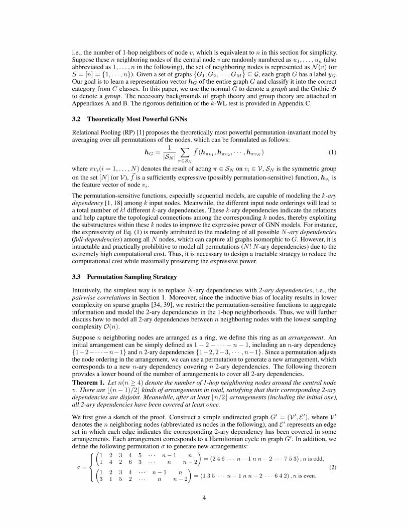
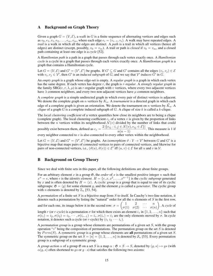
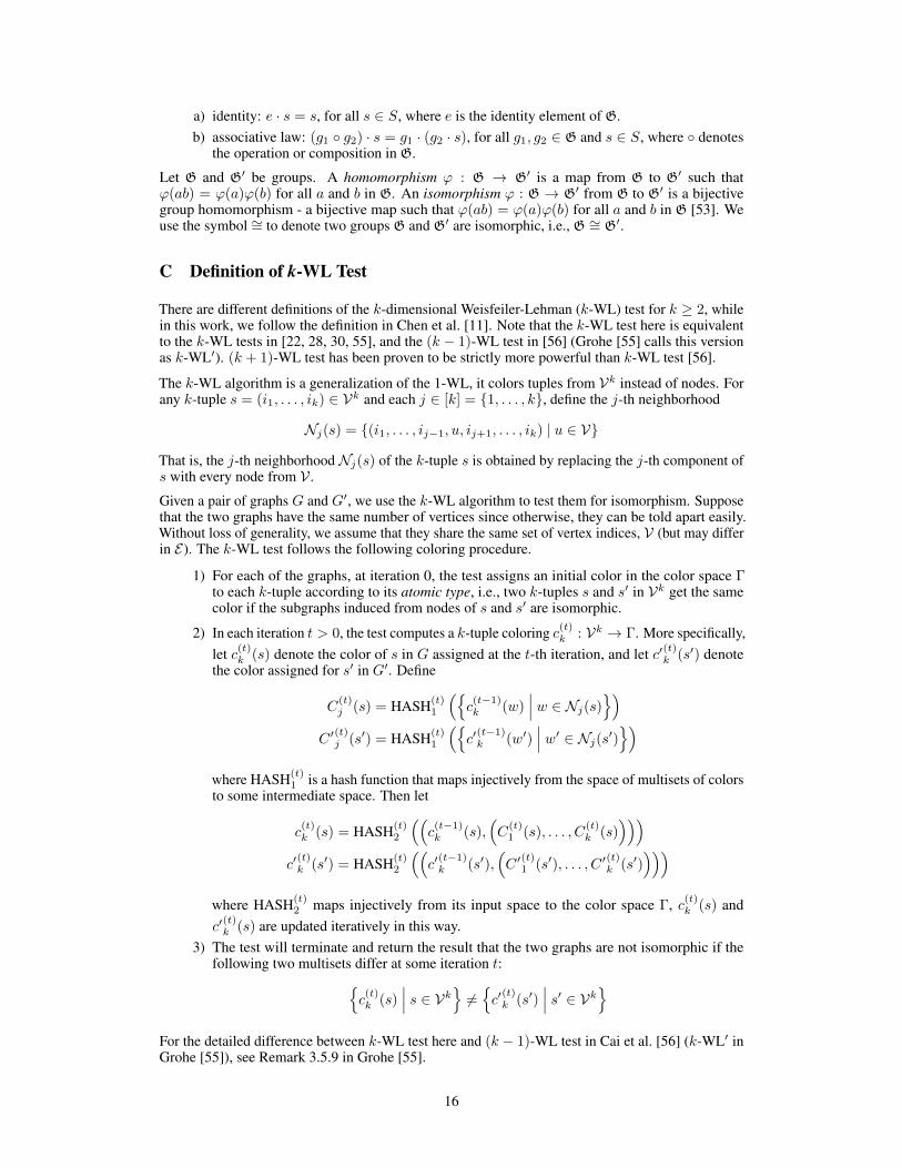
i.e., the number of 1-hop neighbors of node v, which is equivalent to n in this section for simplicity.Suppose these n neighboring nodes of the central node v are randomly numbered as u1, . . . , un (alsoabbreviated as 1, . . . , n in the following), the set of neighboring nodes is represented as N (v) (orS = [n] = 1, . . . , n). Given a set of graphs G1, G2, . . . , GM ⊆ G, each graph G has a label yG.Our goal is to learn a representation vector hG of the entire graph G and classify it into the correctcategory from C classes. In this paper, we use the normal G to denote a graph and the Gothic Gto denote a group. The necessary backgrounds of graph theory and group theory are attached inAppendixes A and B. The rigorous definition of the k-WL test is provided in Appendix C.

3.2 Theoretically Most Powerful GNNs

Relational Pooling (RP) [1] proposes the theoretically most powerful permutation-invariant model byaveraging over all permutations of the nodes, which can be formulated as follows:

hG =1

|SN |∑π∈SN

~f (hπv1 ,hπv2 , · · · ,hπvN ) (1)

where πvi(i = 1, . . . , N) denotes the result of acting π ∈ SN on vi ∈ V , SN is the symmetric groupon the set [N ] (or V), ~f is a sufficiently expressive (possibly permutation-sensitive) function, hvi isthe feature vector of node vi.

The permutation-sensitive functions, especially sequential models, are capable of modeling the k-arydependency [1, 18] among k input nodes. Meanwhile, the different input node orderings will lead toa total number of k! different k-ary dependencies. These k-ary dependencies indicate the relationsand help capture the topological connections among the corresponding k nodes, thereby exploitingthe substructures within these k nodes to improve the expressive power of GNN models. For instance,the expressivity of Eq. (1) is mainly attributed to the modeling of all possible N -ary dependencies(full-dependencies) among all N nodes, which can capture all graphs isomorphic to G. However, it isintractable and practically prohibitive to model all permutations (N ! N -ary dependencies) due to theextremely high computational cost. Thus, it is necessary to design a tractable strategy to reduce thecomputational cost while maximally preserving the expressive power.

3.3 Permutation Sampling Strategy

Intuitively, the simplest way is to replace N -ary dependencies with 2-ary dependencies, i.e., thepairwise correlations in Section 1. Moreover, since the inductive bias of locality results in lowercomplexity on sparse graphs [34, 39], we restrict the permutation-sensitive functions to aggregateinformation and model the 2-ary dependencies in the 1-hop neighborhoods. Thus, we will furtherdiscuss how to model all 2-ary dependencies between n neighboring nodes with the lowest samplingcomplexity O(n).

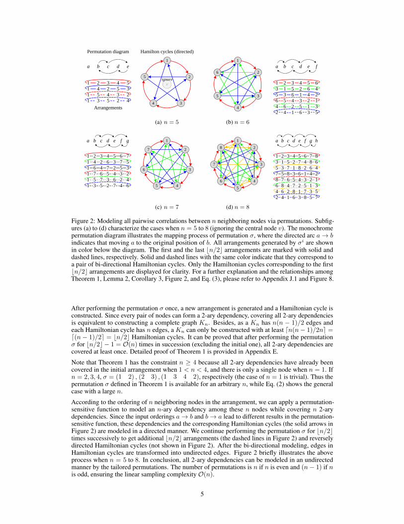
Suppose n neighboring nodes are arranged as a ring, we define this ring as an arrangement. Aninitial arrangement can be simply defined as 1− 2− · · · − n− 1, including an n-ary dependency1−2−· · ·−n−1 and n 2-ary dependencies 1−2, 2−3, · · · , n−1. Since a permutation adjuststhe node ordering in the arrangement, we can use a permutation to generate a new arrangement, whichcorresponds to a new n-ary dependency covering n 2-ary dependencies. The following theoremprovides a lower bound of the number of arrangements to cover all 2-ary dependencies.Theorem 1. Let n(n ≥ 4) denote the number of 1-hop neighboring nodes around the central nodev. There are b(n− 1)/2c kinds of arrangements in total, satisfying that their corresponding 2-arydependencies are disjoint. Meanwhile, after at least bn/2c arrangements (including the initial one),all 2-ary dependencies have been covered at least once.

We first give a sketch of the proof. Construct a simple undirected graph G′ = (V ′, E ′), where V ′denotes the n neighboring nodes (abbreviated as nodes in the following), and E ′ represents an edgeset in which each edge indicates the corresponding 2-ary dependency has been covered in somearrangements. Each arrangement corresponds to a Hamiltonian cycle in graph G′. In addition, wedefine the following permutation σ to generate new arrangements:

σ =

(

1 2 3 4 5 · · · n− 1 n1 4 2 6 3 · · · n n− 2

)= (2 4 6 · · · n− 1 n n− 2 · · · 7 5 3) , n is odd,(

1 2 3 4 · · · n− 1 n3 1 5 2 · · · n n− 2

)= (1 3 5 · · · n− 1 n n− 2 · · · 6 4 2) , n is even.

(2)

4

a b c d e

1 2 3 4 5

1 4 2 5 3

1 5 4 3 2

1 3 5 2 4

1

25

34

a b c d e f

1 2 3 4 5 6

3 1 5 2 6 4

5 3 6 1 4 2

6 5 4 3 2 1

4 6 2 5 1 3

2 4 1 6 3 5

1

2

3

4

5

6

Permutation diagram Hamilton cycles (directed)

Arrangements

vignore

(a) n = 5 (b) n = 6

1

27

36

45

a b c d e f g

1 2 3 4 5 6 7

1 4 2 6 3 7 5

1 6 4 7 2 5 3

1 7 6 5 4 3 2

1 5 7 3 6 2 4

1 3 5 2 7 4 6

a b c d e f g h

1 2 3 4 5 6 7 8

8 7 6 5 4 3 2 1

6 8 4 7 2 5 1 3

4 6 2 8 1 7 3 5

2 4 1 6 3 8 5 7

7 5 8 3 6 1 4 2

5 3 7 1 8 2 6 4

3 1 5 2 7 4 8 6

1

2

3

4

5

6

7

8

(c) n = 7 (d) n = 8

Figure 2: Modeling all pairwise correlations between n neighboring nodes via permutations. Subfig-ures (a) to (d) characterize the cases when n = 5 to 8 (ignoring the central node v). The monochromepermutation diagram illustrates the mapping process of permutation σ, where the directed arc a→ bindicates that moving a to the original position of b. All arrangements generated by σi are shownin color below the diagram. The first and the last bn/2c arrangements are marked with solid anddashed lines, respectively. Solid and dashed lines with the same color indicate that they correspond toa pair of bi-directional Hamiltonian cycles. Only the Hamiltonian cycles corresponding to the firstbn/2c arrangements are displayed for clarity. For a further explanation and the relationships amongTheorem 1, Lemma 2, Corollary 3, Figure 2, and Eq. (3), please refer to Appendix J.1 and Figure 8.

After performing the permutation σ once, a new arrangement is generated and a Hamiltonian cycle isconstructed. Since every pair of nodes can form a 2-ary dependency, covering all 2-ary dependenciesis equivalent to constructing a complete graph Kn. Besides, as a Kn has n(n − 1)/2 edges andeach Hamiltonian cycle has n edges, a Kn can only be constructed with at least dn(n− 1)/2ne =d(n− 1)/2e = bn/2c Hamiltonian cycles. It can be proved that after performing the permutationσ for bn/2c − 1 = O(n) times in succession (excluding the initial one), all 2-ary dependencies arecovered at least once. Detailed proof of Theorem 1 is provided in Appendix E.

Note that Theorem 1 has the constraint n ≥ 4 because all 2-ary dependencies have already beencovered in the initial arrangement when 1 < n < 4, and there is only a single node when n = 1. Ifn = 2, 3, 4, σ = (1 2) , (2 3) , (1 3 4 2), respectively (the case of n = 1 is trivial). Thus thepermutation σ defined in Theorem 1 is available for an arbitrary n, while Eq. (2) shows the generalcase with a large n.

According to the ordering of n neighboring nodes in the arrangement, we can apply a permutation-sensitive function to model an n-ary dependency among these n nodes while covering n 2-arydependencies. Since the input orderings a→ b and b→ a lead to different results in the permutation-sensitive function, these dependencies and the corresponding Hamiltonian cycles (the solid arrows inFigure 2) are modeled in a directed manner. We continue performing the permutation σ for bn/2ctimes successively to get additional bn/2c arrangements (the dashed lines in Figure 2) and reverselydirected Hamiltonian cycles (not shown in Figure 2). After the bi-directional modeling, edges inHamiltonian cycles are transformed into undirected edges. Figure 2 briefly illustrates the aboveprocess when n = 5 to 8. In conclusion, all 2-ary dependencies can be modeled in an undirectedmanner by the tailored permutations. The number of permutations is n if n is even and (n− 1) if nis odd, ensuring the linear sampling complexity O(n).

5

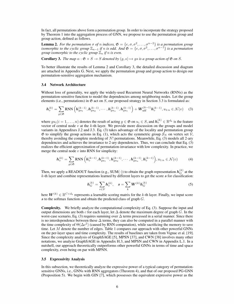
In fact, all permutations above form a permutation group. In order to incorporate the strategy proposedby Theorem 1 into the aggregation process of GNN, we propose to use the permutation group andgroup action, defined as follows.Lemma 2. For the permutation σ of n indices, G = e, σ, σ2, . . . , σn−2 is a permutation groupisomorphic to the cyclic group Zn−1 if n is odd. And G = e, σ, σ2, . . . , σn−1 is a permutationgroup isomorphic to the cyclic group Zn if n is even.

Corollary 3. The map α : G× S → S denoted by (g, s) 7→ gs is a group action of G on S.

To better illustrate the results of Lemma 2 and Corollary 3, the detailed discussion and diagramare attached in Appendix G. Next, we apply the permutation group and group action to design ourpermutation-sensitive aggregation mechanism.

3.4 Network Architecture

Without loss of generality, we apply the widely-used Recurrent Neural Networks (RNNs) as thepermutation-sensitive function to model the dependencies among neighboring nodes. Let the groupelements (i.e., permutations) in G act on S, our proposed strategy in Section 3.3 is formulated as:

h(k)v =

∑g∈G

RNN(h(k−1)gu1

,h(k−1)gu2

, · · · ,h(k−1)gun

,h(k−1)gu1

)+W

(k−1)self h(k−1)

v , u1:n ∈ N (v) (3)

where gui(i = 1, . . . , n) denotes the result of acting g ∈ G on ui ∈ S, and h(k)v ∈ Rdk is the feature

vector of central node v at the k-th layer. We provide more discussion on the groups and modelvariants in Appendixes J.2 and J.3. Eq. (3) takes advantage of the locality and permutation groupG to simplify the group actions in Eq. (1), which acts the symmetric group SN on vertex set V ,thereby avoiding the complete modeling of N ! permutations. Meanwhile, Eq. (3) models all 2-arydependencies and achieves the invariance to 2-ary dependencies. Thus, we can conclude that Eq. (3)realizes the efficient approximation of permutation-invariance with low complexity. In practice, wemerge the central node v into RNN for simplicity:

h(k)v =

∑g∈G

RNN(h(k−1)v ,h(k−1)

gu1,h(k−1)

gu2, · · · ,h(k−1)

gun,h(k−1)

v

), u1:n ∈ N (v) (4)

Then, we apply a READOUT function (e.g., SUM(·)) to obtain the graph representation h(k)G at the

k-th layer and combine representations learned by different layers to get the score s for classification:

h(k)G =

∑v∈V

h(k)v , s =

∑k

W (k)h(k)G (5)

hereW (k) ∈ RC×dk represents a learnable scoring matrix for the k-th layer. Finally, we input scores to the softmax function and obtain the predicted class of graph G.

Complexity. We briefly analyze the computational complexity of Eq. (3). Suppose the input andoutput dimensions are both c for each layer, let ∆ denote the maximum degree of graph G. In theworst-case scenario, Eq. (3) requires summing over ∆ terms processed in a serial manner. Since thereis no interdependence between these ∆ terms, they can also be computed in a parallel manner withthe time complexity of Θ(∆c2) (caused by RNN computation), while sacrificing the memory to savetime. Let M denote the number of edges. Table 1 compares our approach with other powerful GNNson the per-layer space and time complexity. The results of baselines are taken from Vignac et al. [19].Since the complexity analysis of GraphSAGE [5], MPSN [37], and CWN [38] involves many othernotations, we analyze GraphSAGE in Appendix H.3, and MPSN and CWN in Appendix L.1. In anutshell, our approach theoretically outperforms other powerful GNNs in terms of time and spacecomplexity, even being on par with MPNN.

3.5 Expressivity Analysis

In this subsection, we theoretically analyze the expressive power of a typical category of permutation-sensitive GNNs, i.e., GNNs with RNN aggregators (Theorem 4), and that of our proposed PG-GNN(Proposition 5). We begin with GIN [7], which possesses the equivalent expressive power as the

6

Table 1: Memory and time complexity per layer.

Model Memory Time complexity

GIN [7] Θ(Nc) Θ(Mc+Nc2)MPNN [4] Θ(Nc) Θ(Mc2)Fast SMP [19] Θ(N2c) Θ(MNc+N2c2)SMP [19] Θ(N2c) Θ(MNc2)PPGN [28] Θ(N2c) Θ(N3c+N2c2)3-WL [22] Θ(N3c) Θ(N4c+N3c2)

Ours (serial) Θ(Nc) Θ(N∆2c2)Ours (parallel) Θ(N∆c) Θ(N∆c2)

Table 2: Results (measured by MAE) on inci-dence triangle counting.

Model Erdos-Rényirandom graph

Randomregular graph

GCN [3] 0.599 ± 0.006 0.500 ± 0.012SAGE [5] 0.118 ± 0.005 0.127 ± 0.011GIN [7] 0.219 ± 0.016 0.342 ± 0.005rGIN [25] 0.194 ± 0.009 0.325 ± 0.006RP [1] 0.058 ± 0.006 0.161 ± 0.003LRP [11] 0.023 ± 0.011 0.037 ± 0.019

PG-GNN 0.019 ± 0.002 0.027 ± 0.001

2-WL test [7, 30]. In fact, the variants of GIN can be recovered by GNNs with RNN aggregators (seeAppendix I for details), which implies that this category of permutation-sensitive GNNs can be atleast as powerful as the 2-WL test. Next, we explicate why they go beyond the 2-WL test from theperspective of substructure counting.

Triangular substructures are rich in various networks, and counting triangles is an important task innetwork analysis [40]. For example, in social networks, the formation of a triangle indicates that twopeople with a common friend will also become friends [41]. A triangle4uivuj is incident to the nodev if ui and uj are adjacent and node v is their common neighbor. We define the triangle4uivuj asan incidence triangle over node v (also ui and uj), and denote the number of incidence triangles overnode v as τv . Formally, the number of incidence triangles over each node in an undirected graph canbe calculated as follows (proof and discussion for the directed graph are provided in Appendix H.1):

τ =1

2A2 A · 1N (6)

where τ ∈ RN and its i-th element τi represents the number of incidence triangles over node i, denotes element-wise product (i.e., Hadamard product), 1N = (1, 1, · · · , 1)> ∈ RN is a sum vector.

Besides the WL-test, the capability of counting graph substructures also characterizes the expressivepower of GNNs [11]. Thus, we verify the expressivity of permutation-sensitive GNNs by evaluatingtheir abilities to count triangles.Theorem 4. Let xv,∀v ∈ V denote the feature inputs on graph G = (V, E), and M be a generalGNN model with RNN aggregators. Suppose that xv is initialized as the degree dv of node v, andeach node is distinguishable. For any 0 < ε ≤ 1/8 and 0 < δ < 1, there exists a parameter setting

Θ for M so that after O(dv(2dv+τv)t

dv+τv

)samples,

Pr

(∣∣∣∣zvτv − 1

∣∣∣∣ ≤ ε) ≥ 1− δ, ∀v ∈ V,

where zv ∈ R is the final output value generated by M and τv is the number of incidence triangles.

Detailed proof can be found in Appendix H.2. Theorem 4 concludes that, if the input node featuresare node degrees and nodes are distinguishable, there exists a parameter setting for a general GNNwith RNN aggregators such that it can approximate the number of incidence triangles to arbitraryprecision for every node. Since 2-WL and MPNNs cannot count triangles [11], we conclude that thiscategory of permutation-sensitive GNNs is more powerful. However, the required samples are relatedto τv and proportional to the mixing time t (see Appendix H.2), leading to a practically prohibitiveaggregation complexity. Many existing permutation-sensitive GNNs like GraphSAGE with LSTMand RP with π-SGD suffer from this issue (see Appendixes H.3 and K.2 for more discussion).

On the contrary, our approach can estimate the number of incidence triangles in linear samplingcomplexity O(n) = O(dv). According to the definition of incidence triangles and the fact that theyalways appear within v’s 1-hop neighborhood, we know that the number of connections betweenthe central node v’s neighboring nodes is equivalent to the number of incidence triangles over v.Meanwhile, Theorem 1 and Eq. (3) ensure that all 2-ary dependencies between n neighboring nodesare modeled withO(n) sampling complexity. These dependencies capture the information of whether

7

two neighboring nodes are connected, thereby estimating the number of connections and countingincidence triangles in linear sampling complexity.

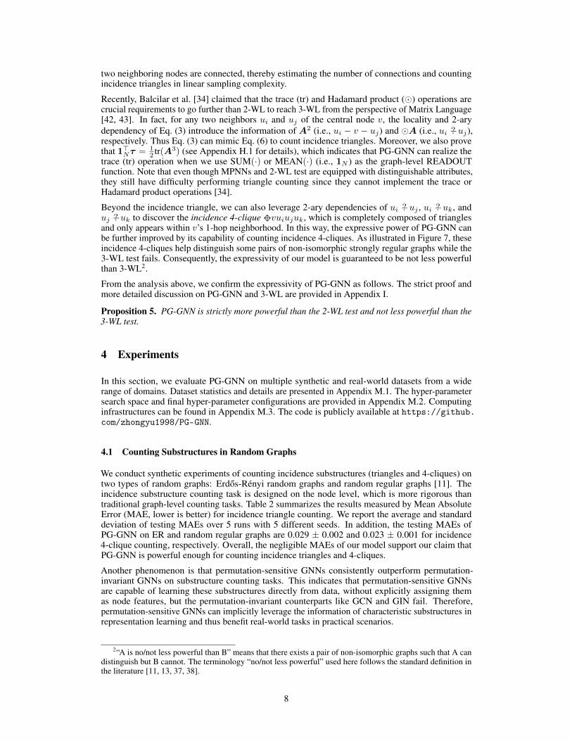
Recently, Balcilar et al. [34] claimed that the trace (tr) and Hadamard product () operations arecrucial requirements to go further than 2-WL to reach 3-WL from the perspective of Matrix Language[42, 43]. In fact, for any two neighbors ui and uj of the central node v, the locality and 2-arydependency of Eq. (3) introduce the information of A2 (i.e., ui − v − uj) and A (i.e., ui −? uj),respectively. Thus Eq. (3) can mimic Eq. (6) to count incidence triangles. Moreover, we also provethat 1>Nτ = 1

2 tr(A3) (see Appendix H.1 for details), which indicates that PG-GNN can realize thetrace (tr) operation when we use SUM(·) or MEAN(·) (i.e., 1N ) as the graph-level READOUTfunction. Note that even though MPNNs and 2-WL test are equipped with distinguishable attributes,they still have difficulty performing triangle counting since they cannot implement the trace orHadamard product operations [34].

Beyond the incidence triangle, we can also leverage 2-ary dependencies of ui −? uj , ui −? uk, anduj −? uk to discover the incidence 4-clique |vuiujuk, which is completely composed of trianglesand only appears within v’s 1-hop neighborhood. In this way, the expressive power of PG-GNN canbe further improved by its capability of counting incidence 4-cliques. As illustrated in Figure 7, theseincidence 4-cliques help distinguish some pairs of non-isomorphic strongly regular graphs while the3-WL test fails. Consequently, the expressivity of our model is guaranteed to be not less powerfulthan 3-WL2.

From the analysis above, we confirm the expressivity of PG-GNN as follows. The strict proof andmore detailed discussion on PG-GNN and 3-WL are provided in Appendix I.

Proposition 5. PG-GNN is strictly more powerful than the 2-WL test and not less powerful than the3-WL test.

4 Experiments

In this section, we evaluate PG-GNN on multiple synthetic and real-world datasets from a widerange of domains. Dataset statistics and details are presented in Appendix M.1. The hyper-parametersearch space and final hyper-parameter configurations are provided in Appendix M.2. Computinginfrastructures can be found in Appendix M.3. The code is publicly available at https://github.com/zhongyu1998/PG-GNN.

4.1 Counting Substructures in Random Graphs

We conduct synthetic experiments of counting incidence substructures (triangles and 4-cliques) ontwo types of random graphs: Erdos-Rényi random graphs and random regular graphs [11]. Theincidence substructure counting task is designed on the node level, which is more rigorous thantraditional graph-level counting tasks. Table 2 summarizes the results measured by Mean AbsoluteError (MAE, lower is better) for incidence triangle counting. We report the average and standarddeviation of testing MAEs over 5 runs with 5 different seeds. In addition, the testing MAEs ofPG-GNN on ER and random regular graphs are 0.029 ± 0.002 and 0.023 ± 0.001 for incidence4-clique counting, respectively. Overall, the negligible MAEs of our model support our claim thatPG-GNN is powerful enough for counting incidence triangles and 4-cliques.

Another phenomenon is that permutation-sensitive GNNs consistently outperform permutation-invariant GNNs on substructure counting tasks. This indicates that permutation-sensitive GNNsare capable of learning these substructures directly from data, without explicitly assigning themas node features, but the permutation-invariant counterparts like GCN and GIN fail. Therefore,permutation-sensitive GNNs can implicitly leverage the information of characteristic substructures inrepresentation learning and thus benefit real-world tasks in practical scenarios.

2“A is no/not less powerful than B” means that there exists a pair of non-isomorphic graphs such that A candistinguish but B cannot. The terminology “no/not less powerful” used here follows the standard definition inthe literature [11, 13, 37, 38].

8

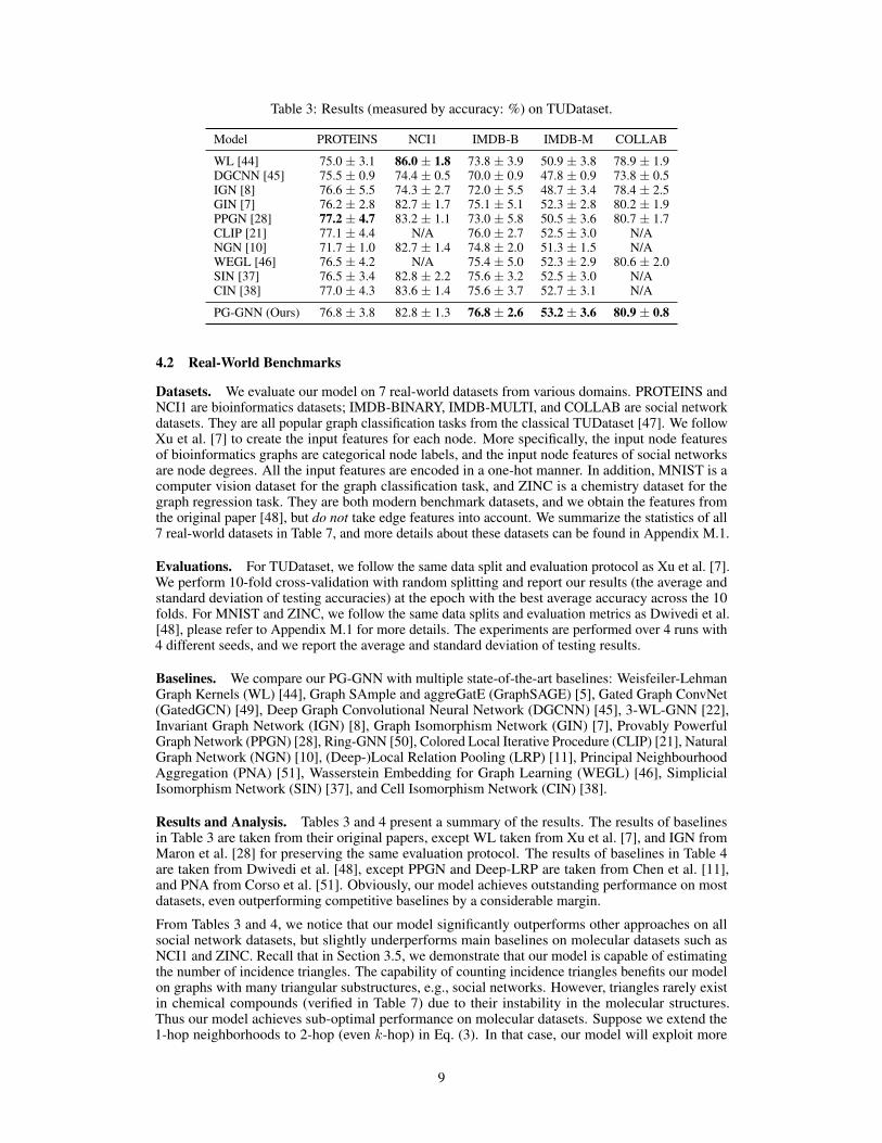
Table 3: Results (measured by accuracy: %) on TUDataset.

Model PROTEINS NCI1 IMDB-B IMDB-M COLLAB

WL [44] 75.0 ± 3.1 86.0 ± 1.8 73.8 ± 3.9 50.9 ± 3.8 78.9 ± 1.9DGCNN [45] 75.5 ± 0.9 74.4 ± 0.5 70.0 ± 0.9 47.8 ± 0.9 73.8 ± 0.5IGN [8] 76.6 ± 5.5 74.3 ± 2.7 72.0 ± 5.5 48.7 ± 3.4 78.4 ± 2.5GIN [7] 76.2 ± 2.8 82.7 ± 1.7 75.1 ± 5.1 52.3 ± 2.8 80.2 ± 1.9PPGN [28] 77.2 ± 4.7 83.2 ± 1.1 73.0 ± 5.8 50.5 ± 3.6 80.7 ± 1.7CLIP [21] 77.1 ± 4.4 N/A 76.0 ± 2.7 52.5 ± 3.0 N/ANGN [10] 71.7 ± 1.0 82.7 ± 1.4 74.8 ± 2.0 51.3 ± 1.5 N/AWEGL [46] 76.5 ± 4.2 N/A 75.4 ± 5.0 52.3 ± 2.9 80.6 ± 2.0SIN [37] 76.5 ± 3.4 82.8 ± 2.2 75.6 ± 3.2 52.5 ± 3.0 N/ACIN [38] 77.0 ± 4.3 83.6 ± 1.4 75.6 ± 3.7 52.7 ± 3.1 N/A

PG-GNN (Ours) 76.8 ± 3.8 82.8 ± 1.3 76.8 ± 2.6 53.2 ± 3.6 80.9 ± 0.8

4.2 Real-World Benchmarks

Datasets. We evaluate our model on 7 real-world datasets from various domains. PROTEINS andNCI1 are bioinformatics datasets; IMDB-BINARY, IMDB-MULTI, and COLLAB are social networkdatasets. They are all popular graph classification tasks from the classical TUDataset [47]. We followXu et al. [7] to create the input features for each node. More specifically, the input node featuresof bioinformatics graphs are categorical node labels, and the input node features of social networksare node degrees. All the input features are encoded in a one-hot manner. In addition, MNIST is acomputer vision dataset for the graph classification task, and ZINC is a chemistry dataset for thegraph regression task. They are both modern benchmark datasets, and we obtain the features fromthe original paper [48], but do not take edge features into account. We summarize the statistics of all7 real-world datasets in Table 7, and more details about these datasets can be found in Appendix M.1.

Evaluations. For TUDataset, we follow the same data split and evaluation protocol as Xu et al. [7].We perform 10-fold cross-validation with random splitting and report our results (the average andstandard deviation of testing accuracies) at the epoch with the best average accuracy across the 10folds. For MNIST and ZINC, we follow the same data splits and evaluation metrics as Dwivedi et al.[48], please refer to Appendix M.1 for more details. The experiments are performed over 4 runs with4 different seeds, and we report the average and standard deviation of testing results.

Baselines. We compare our PG-GNN with multiple state-of-the-art baselines: Weisfeiler-LehmanGraph Kernels (WL) [44], Graph SAmple and aggreGatE (GraphSAGE) [5], Gated Graph ConvNet(GatedGCN) [49], Deep Graph Convolutional Neural Network (DGCNN) [45], 3-WL-GNN [22],Invariant Graph Network (IGN) [8], Graph Isomorphism Network (GIN) [7], Provably PowerfulGraph Network (PPGN) [28], Ring-GNN [50], Colored Local Iterative Procedure (CLIP) [21], NaturalGraph Network (NGN) [10], (Deep-)Local Relation Pooling (LRP) [11], Principal NeighbourhoodAggregation (PNA) [51], Wasserstein Embedding for Graph Learning (WEGL) [46], SimplicialIsomorphism Network (SIN) [37], and Cell Isomorphism Network (CIN) [38].

Results and Analysis. Tables 3 and 4 present a summary of the results. The results of baselinesin Table 3 are taken from their original papers, except WL taken from Xu et al. [7], and IGN fromMaron et al. [28] for preserving the same evaluation protocol. The results of baselines in Table 4are taken from Dwivedi et al. [48], except PPGN and Deep-LRP are taken from Chen et al. [11],and PNA from Corso et al. [51]. Obviously, our model achieves outstanding performance on mostdatasets, even outperforming competitive baselines by a considerable margin.

From Tables 3 and 4, we notice that our model significantly outperforms other approaches on allsocial network datasets, but slightly underperforms main baselines on molecular datasets such asNCI1 and ZINC. Recall that in Section 3.5, we demonstrate that our model is capable of estimatingthe number of incidence triangles. The capability of counting incidence triangles benefits our modelon graphs with many triangular substructures, e.g., social networks. However, triangles rarely existin chemical compounds (verified in Table 7) due to their instability in the molecular structures.Thus our model achieves sub-optimal performance on molecular datasets. Suppose we extend the1-hop neighborhoods to 2-hop (even k-hop) in Eq. (3). In that case, our model will exploit more

9

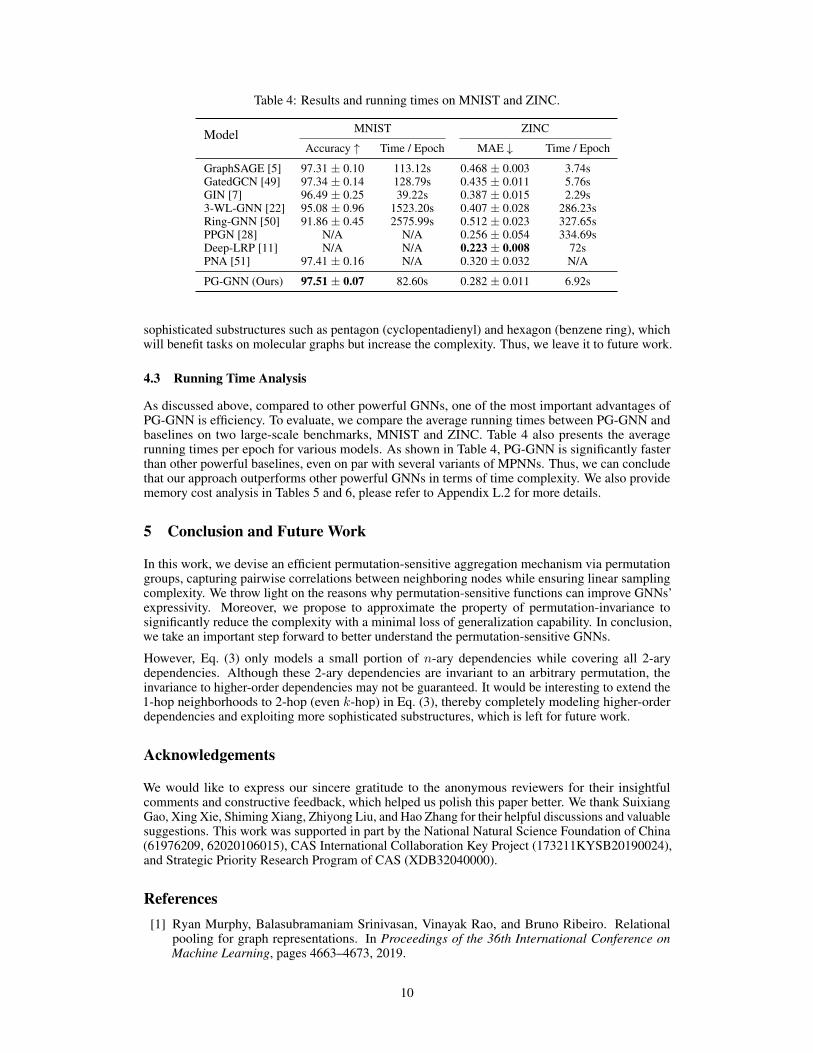
Table 4: Results and running times on MNIST and ZINC.

Model MNIST ZINC

Accuracy ↑ Time / Epoch MAE ↓ Time / Epoch

GraphSAGE [5] 97.31 ± 0.10 113.12s 0.468 ± 0.003 3.74sGatedGCN [49] 97.34 ± 0.14 128.79s 0.435 ± 0.011 5.76sGIN [7] 96.49 ± 0.25 39.22s 0.387 ± 0.015 2.29s3-WL-GNN [22] 95.08 ± 0.96 1523.20s 0.407 ± 0.028 286.23sRing-GNN [50] 91.86 ± 0.45 2575.99s 0.512 ± 0.023 327.65sPPGN [28] N/A N/A 0.256 ± 0.054 334.69sDeep-LRP [11] N/A N/A 0.223 ± 0.008 72sPNA [51] 97.41 ± 0.16 N/A 0.320 ± 0.032 N/A

PG-GNN (Ours) 97.51 ± 0.07 82.60s 0.282 ± 0.011 6.92s

sophisticated substructures such as pentagon (cyclopentadienyl) and hexagon (benzene ring), whichwill benefit tasks on molecular graphs but increase the complexity. Thus, we leave it to future work.

4.3 Running Time Analysis

As discussed above, compared to other powerful GNNs, one of the most important advantages ofPG-GNN is efficiency. To evaluate, we compare the average running times between PG-GNN andbaselines on two large-scale benchmarks, MNIST and ZINC. Table 4 also presents the averagerunning times per epoch for various models. As shown in Table 4, PG-GNN is significantly fasterthan other powerful baselines, even on par with several variants of MPNNs. Thus, we can concludethat our approach outperforms other powerful GNNs in terms of time complexity. We also providememory cost analysis in Tables 5 and 6, please refer to Appendix L.2 for more details.

5 Conclusion and Future Work

In this work, we devise an efficient permutation-sensitive aggregation mechanism via permutationgroups, capturing pairwise correlations between neighboring nodes while ensuring linear samplingcomplexity. We throw light on the reasons why permutation-sensitive functions can improve GNNs’expressivity. Moreover, we propose to approximate the property of permutation-invariance tosignificantly reduce the complexity with a minimal loss of generalization capability. In conclusion,we take an important step forward to better understand the permutation-sensitive GNNs.

However, Eq. (3) only models a small portion of n-ary dependencies while covering all 2-arydependencies. Although these 2-ary dependencies are invariant to an arbitrary permutation, theinvariance to higher-order dependencies may not be guaranteed. It would be interesting to extend the1-hop neighborhoods to 2-hop (even k-hop) in Eq. (3), thereby completely modeling higher-orderdependencies and exploiting more sophisticated substructures, which is left for future work.

Acknowledgements

We would like to express our sincere gratitude to the anonymous reviewers for their insightfulcomments and constructive feedback, which helped us polish this paper better. We thank SuixiangGao, Xing Xie, Shiming Xiang, Zhiyong Liu, and Hao Zhang for their helpful discussions and valuablesuggestions. This work was supported in part by the National Natural Science Foundation of China(61976209, 62020106015), CAS International Collaboration Key Project (173211KYSB20190024),and Strategic Priority Research Program of CAS (XDB32040000).

References[1] Ryan Murphy, Balasubramaniam Srinivasan, Vinayak Rao, and Bruno Ribeiro. Relational

pooling for graph representations. In Proceedings of the 36th International Conference onMachine Learning, pages 4663–4673, 2019.

10

[2] David Duvenaud, Dougal Maclaurin, Jorge Aguilera-Iparraguirre, Rafael Gómez-Bombarelli,Timothy Hirzel, Alán Aspuru-Guzik, and Ryan P Adams. Convolutional networks on graphsfor learning molecular fingerprints. In Advances in Neural Information Processing Systems,pages 2224–2232, 2015.

[3] Thomas N Kipf and Max Welling. Semi-supervised classification with graph convolutionalnetworks. In Proceedings of the 5th International Conference on Learning Representations,2017.

[4] Justin Gilmer, Samuel S Schoenholz, Patrick F Riley, Oriol Vinyals, and George E Dahl. Neuralmessage passing for quantum chemistry. In Proceedings of the 34th International Conferenceon Machine Learning, pages 1263–1272, 2017.

[5] William L Hamilton, Rex Ying, and Jure Leskovec. Inductive representation learning on largegraphs. In Advances in Neural Information Processing Systems, pages 1024–1034, 2017.

[6] Rex Ying, Jiaxuan You, Christopher Morris, Xiang Ren, William L Hamilton, and Jure Leskovec.Hierarchical graph representation learning with differentiable pooling. In Advances in NeuralInformation Processing Systems, pages 4800–4810, 2018.

[7] Keyulu Xu, Weihua Hu, Jure Leskovec, and Stefanie Jegelka. How powerful are graph neuralnetworks? In Proceedings of the 7th International Conference on Learning Representations,2019.

[8] Haggai Maron, Heli Ben-Hamu, Nadav Shamir, and Yaron Lipman. Invariant and equivariantgraph networks. In Proceedings of the 7th International Conference on Learning Representa-tions, 2019.

[9] Risi Kondor, Hy Truong Son, Horace Pan, Brandon Anderson, and Shubhendu Trivedi. Covari-ant compositional networks for learning graphs. arXiv preprint arXiv:1801.02144, 2018.

[10] Pim de Haan, Taco Cohen, and Max Welling. Natural graph networks. In Advances in NeuralInformation Processing Systems, pages 3636–3646, 2020.

[11] Zhengdao Chen, Lei Chen, Soledad Villar, and Joan Bruna. Can graph neural networks countsubstructures? In Advances in Neural Information Processing Systems, pages 10383–10395,2020.

[12] Erik Henning Thiede, Wenda Zhou, and Risi Kondor. Autobahn: Automorphism-based graphneural nets. In Advances in Neural Information Processing Systems, pages 29922–29934, 2021.

[13] Lingxiao Zhao, Wei Jin, Leman Akoglu, and Neil Shah. From stars to subgraphs: Uplifting anyGNN with local structure awareness. In Proceedings of the 10th International Conference onLearning Representations, 2022.

[14] Beatrice Bevilacqua, Fabrizio Frasca, Derek Lim, Balasubramaniam Srinivasan, Chen Cai,Gopinath Balamurugan, Michael M Bronstein, and Haggai Maron. Equivariant subgraphaggregation networks. In Proceedings of the 10th International Conference on LearningRepresentations, 2022.

[15] Jeffrey L Elman. Finding structure in time. Cognitive Science, 14(2):179–211, 1990.

[16] Kyunghyun Cho, Bart van Merriënboer, Caglar Gulcehre, Dzmitry Bahdanau, Fethi Bougares,Holger Schwenk, and Yoshua Bengio. Learning phrase representations using RNN encoder-decoder for statistical machine translation. In Proceedings of the 2014 Conference on EmpiricalMethods in Natural Language Processing, pages 1724–1734, 2014.

[17] Sepp Hochreiter and Jürgen Schmidhuber. Long short-term memory. Neural computation, 9(8):1735–1780, 1997.

[18] Ryan L Murphy, Balasubramaniam Srinivasan, Vinayak Rao, and Bruno Ribeiro. Janossypooling: Learning deep permutation-invariant functions for variable-size inputs. In Proceedingsof the 7th International Conference on Learning Representations, 2019.

11

[19] Clément Vignac, Andreas Loukas, and Pascal Frossard. Building powerful and equivariantgraph neural networks with structural message-passing. In Advances in Neural InformationProcessing Systems, pages 14143–14155, 2020.

[20] Andreas Loukas. What graph neural networks cannot learn: Depth vs width. In Proceedings ofthe 8th International Conference on Learning Representations, 2020.

[21] George Dasoulas, Ludovic Dos Santos, Kevin Scaman, and Aladin Virmaux. Coloring graphneural networks for node disambiguation. In Proceedings of the 29th International JointConference on Artificial Intelligence, pages 2126–2132, 2020.

[22] Christopher Morris, Martin Ritzert, Matthias Fey, William L Hamilton, Jan Eric Lenssen, GauravRattan, and Martin Grohe. Weisfeiler and Leman go neural: Higher-order graph neural networks.In Proceedings of the 33rd AAAI Conference on Artificial Intelligence, pages 4602–4609, 2019.

[23] Boris Weisfeiler and Andrei A Leman. A reduction of a graph to a canonical form and analgebra arising during this reduction. Nauchno-Technicheskaya Informatsiya, 2(9):12–16, 1968.

[24] Ryoma Sato, Makoto Yamada, and Hisashi Kashima. Approximation ratios of graph neuralnetworks for combinatorial problems. In Advances in Neural Information Processing Systems,pages 4081–4090, 2019.

[25] Ryoma Sato, Makoto Yamada, and Hisashi Kashima. Random features strengthen graph neuralnetworks. In Proceedings of the 2021 SIAM International Conference on Data Mining, pages333–341, 2021.

[26] Ralph Abboud, Ismail Ilkan Ceylan, Martin Grohe, and Thomas Lukasiewicz. The surprisingpower of graph neural networks with random node initialization. In Proceedings of the 30thInternational Joint Conference on Artificial Intelligence, pages 2112–2118, 2021.

[27] Haggai Maron, Ethan Fetaya, Nimrod Segol, and Yaron Lipman. On the universality of invariantnetworks. In Proceedings of the 36th International Conference on Machine Learning, pages4363–4371, 2019.

[28] Haggai Maron, Heli Ben-Hamu, Hadar Serviansky, and Yaron Lipman. Provably powerfulgraph networks. In Advances in Neural Information Processing Systems, pages 2156–2167,2019.

[29] Nicolas Keriven and Gabriel Peyré. Universal invariant and equivariant graph neural networks.In Advances in Neural Information Processing Systems, pages 7092–7101, 2019.

[30] Waïss Azizian and Marc Lelarge. Expressive power of invariant and equivariant graph neuralnetworks. In Proceedings of the 9th International Conference on Learning Representations,2021.

[31] Vikas Garg, Stefanie Jegelka, and Tommi Jaakkola. Generalization and representational limitsof graph neural networks. In Proceedings of the 37th International Conference on MachineLearning, pages 3419–3430, 2020.

[32] Behrooz Tahmasebi, Derek Lim, and Stefanie Jegelka. Counting substructures with higher-ordergraph neural networks: Possibility and impossibility results. arXiv preprint arXiv:2012.03174,2020.

[33] Jiaxuan You, Jonathan Gomes-Selman, Rex Ying, and Jure Leskovec. Identity-aware graphneural networks. In Proceedings of the 35th AAAI Conference on Artificial Intelligence, pages10737–10745, 2021.

[34] Muhammet Balcilar, Pierre Héroux, Benoit Gaüzère, Pascal Vasseur, Sébastien Adam, and PaulHoneine. Breaking the limits of message passing graph neural networks. In Proceedings of the38th International Conference on Machine Learning, pages 599–608, 2021.

[35] Pablo Barceló, Floris Geerts, Juan Reutter, and Maksimilian Ryschkov. Graph neural networkswith local graph parameters. In Advances in Neural Information Processing Systems, pages25280–25293, 2021.

12

[36] Giorgos Bouritsas, Fabrizio Frasca, Stefanos P Zafeiriou, and Michael M Bronstein. Improvinggraph neural network expressivity via subgraph isomorphism counting. IEEE Transactions onPattern Analysis and Machine Intelligence, 2022.

[37] Cristian Bodnar, Fabrizio Frasca, Yuguang Wang, Nina Otter, Guido F Montúfar, Pietro Liò,and Michael Bronstein. Weisfeiler and Lehman go topological: Message passing simplicialnetworks. In Proceedings of the 38th International Conference on Machine Learning, pages1026–1037, 2021.

[38] Cristian Bodnar, Fabrizio Frasca, Nina Otter, Yu Guang Wang, Pietro Liò, Guido F Montúfar,and Michael Bronstein. Weisfeiler and Lehman go cellular: CW networks. In Advances inNeural Information Processing Systems, pages 2625–2640, 2021.

[39] Peter W Battaglia, Jessica B Hamrick, Victor Bapst, Alvaro Sanchez-Gonzalez, Vinícius Flo-res Zambaldi, Mateusz Malinowski, Andrea Tacchetti, David Raposo, Adam Santoro, RyanFaulkner, et al. Relational inductive biases, deep learning, and graph networks. arXiv preprintarXiv:1806.01261, 2018.

[40] Mohammad Al Hasan and Vachik S Dave. Triangle counting in large networks: A review. WileyInterdisciplinary Reviews: Data Mining and Knowledge Discovery, 8(2):e1226, 2018.

[41] Michael Mitzenmacher and Eli Upfal. Probability and computing: Randomization and proba-bilistic techniques in algorithms and data analysis. Cambridge University Press, 2017.

[42] Robert Brijder, Floris Geerts, Jan Van Den Bussche, and Timmy Weerwag. On the expressivepower of query languages for matrices. ACM Transactions on Database Systems, 44(4):1–31,2019.

[43] Floris Geerts. On the expressive power of linear algebra on graphs. Theory of ComputingSystems, 65(1):179–239, 2021.

[44] Nino Shervashidze, Pascal Schweitzer, Erik Jan Van Leeuwen, Kurt Mehlhorn, and Karsten MBorgwardt. Weisfeiler-Lehman graph kernels. Journal of Machine Learning Research, 12(77):2539–2561, 2011.

[45] Muhan Zhang, Zhicheng Cui, Marion Neumann, and Yixin Chen. An end-to-end deep learningarchitecture for graph classification. In Proceedings of the 32nd AAAI Conference on ArtificialIntelligence, pages 4438–4445, 2018.

[46] Soheil Kolouri, Navid Naderializadeh, Gustavo K Rohde, and Heiko Hoffmann. Wassersteinembedding for graph learning. In Proceedings of the 9th International Conference on LearningRepresentations, 2021.

[47] Christopher Morris, Nils M Kriege, Franka Bause, Kristian Kersting, Petra Mutzel, and MarionNeumann. TUDataset: A collection of benchmark datasets for learning with graphs. ICML2020 Workshop on Graph Representation Learning and Beyond (GRL+), 2020. URL www.graphlearning.io.

[48] Vijay Prakash Dwivedi, Chaitanya K Joshi, Thomas Laurent, Yoshua Bengio, and XavierBresson. Benchmarking graph neural networks. arXiv preprint arXiv:2003.00982, 2020.

[49] Xavier Bresson and Thomas Laurent. Residual gated graph convnets. arXiv preprintarXiv:1711.07553, 2017.

[50] Zhengdao Chen, Soledad Villar, Lei Chen, and Joan Bruna. On the equivalence betweengraph isomorphism testing and function approximation with GNNs. In Advances in NeuralInformation Processing Systems, pages 15894–15902, 2019.

[51] Gabriele Corso, Luca Cavalleri, Dominique Beaini, Pietro Liò, and Petar Velickovic. Principalneighbourhood aggregation for graph nets. In Advances in Neural Information ProcessingSystems, pages 13260–13271, 2020.

[52] Douglas Brent West. Introduction to graph theory. Prentice Hall, 2001.

13

[53] Michael Artin. Algebra. Pearson Prentice Hall, 2011.

[54] Garrett Birkhoff and Saunders Mac Lane. A survey of modern algebra. CRC Press, 2017.

[55] Martin Grohe. Descriptive complexity, canonisation, and definable graph structure theory,volume 47. Cambridge University Press, 2017.

[56] Jin-Yi Cai, Martin Fürer, and Neil Immerman. An optimal lower bound on the number ofvariables for graph identification. Combinatorica, 12(4):389–410, 1992.

[57] Narsingh Deo. Graph theory with applications to engineering and computer science. CourierDover Publications, 2017.

[58] Frank Harary and Bennet Manvel. On the number of cycles in a graph. Matematicky casopis,21(1):55–63, 1971.

[59] Kai-Min Chung, Henry Lam, Zhenming Liu, and Michael Mitzenmacher. Chernoff-Hoeffdingbounds for Markov chains: Generalized and simplified. In Proceedings of the 29th InternationalSymposium on Theoretical Aspects of Computer Science, pages 124–135, 2012.

[60] Simon Haykin. Neural networks and learning machines, 3/E. Pearson Education India, 2010.

[61] Xiaowei Chen, Yongkun Li, Pinghui Wang, and John CS Lui. A general framework forestimating graphlet statistics via random walk. Proceedings of the VLDB Endowment, 10(3):253–264, 2016.

[62] Stephen J Hardiman and Liran Katzir. Estimating clustering coefficients and size of socialnetworks via random walk. In Proceedings of the 22nd International Conference on World WideWeb, pages 539–550, 2013.

[63] Yann LeCun, Léon Bottou, Yoshua Bengio, and Patrick Haffner. Gradient-based learningapplied to document recognition. Proceedings of the IEEE, 86(11):2278–2324, 1998.

[64] Radhakrishna Achanta, Appu Shaji, Kevin Smith, Aurelien Lucchi, Pascal Fua, and SabineSüsstrunk. SLIC superpixels compared to state-of-the-art superpixel methods. IEEE Transac-tions on Pattern Analysis and Machine Intelligence, 34(11):2274–2282, 2012.

[65] John J Irwin, Teague Sterling, Michael M Mysinger, Erin S Bolstad, and Ryan G Coleman.ZINC: A free tool to discover chemistry for biology. Journal of Chemical Information andModeling, 52(7):1757–1768, 2012.

[66] Sergey Ioffe and Christian Szegedy. Batch normalization: Accelerating deep network trainingby reducing internal covariate shift. In Proceedings of the 32nd International Conference onMachine Learning, pages 448–456, 2015.

[67] Xavier Glorot and Yoshua Bengio. Understanding the difficulty of training deep feedforwardneural networks. In Proceedings of the 13th International Conference on Artificial Intelligenceand Statistics, pages 249–256, 2010.

[68] Diederik P Kingma and Jimmy Lei Ba. Adam: A method for stochastic optimization. InProceedings of the 3rd International Conference on Learning Representations, 2015.

[69] Aric Hagberg, Pieter Swart, and Daniel S Chult. Exploring network structure, dynamics, andfunction using NetworkX. In Proceedings of the 7th Python in Science Conference, pages11–15, 2008.

[70] Adam Paszke, Sam Gross, Francisco Massa, Adam Lerer, James Bradbury, Gregory Chanan,Trevor Killeen, Zeming Lin, Natalia Gimelshein, Luca Antiga, et al. PyTorch: An imperativestyle, high-performance deep learning library. In Advances in Neural Information ProcessingSystems, pages 8026–8037, 2019.

[71] Minjie Wang, Lingfan Yu, Da Zheng, Quan Gan, Yu Gai, Zihao Ye, Mufei Li, Jinjing Zhou,Qi Huang, Chao Ma, et al. Deep graph library: Towards efficient and scalable deep learning ongraphs. ICLR Workshop on Representation Learning on Graphs and Manifolds, 2019.

14

A Background on Graph Theory

Given a graph G = (V, E), a walk in G is a finite sequence of alternating vertices and edges suchas v0, e1, v1, e2, . . . , em, vm, where each edge ei = (vi−1, vi). A walk may have repeated edges. Atrail is a walk in which all the edges are distinct. A path is a trail in which all vertices (hence alledges) are distinct (except, possibly, v0 = vm). A trail or path is closed if v0 = vm, and a closedpath containing at least one edge is a cycle [52].

A Hamiltonian path is a path in a graph that passes through each vertex exactly once. A Hamiltoniancycle is a cycle in a graph that passes through each vertex exactly once. A Hamiltonian graph is agraph that contains a Hamiltonian cycle.

Let G = (V, E) and G′ = (V ′, E ′) be graphs. If G′ ⊆ G and G′ contains all the edges (vi, vj) ∈ Ewith vi, vj ∈ V ′, then G′ is an induced subgraph of G, and we say that V ′ induces G′ in G.

An empty graph is a graph whose edge-set is empty. A regular graph is a graph in which each vertexhas the same degree. If each vertex has degree r, the graph is r-regular. A strongly regular graph inthe family SRG(v, r, λ, µ) is an r-regular graph with v vertices, where every two adjacent verticeshave λ common neighbors, and every two non-adjacent vertices have µ common neighbors.

A complete graph is a simple undirected graph in which every pair of distinct vertices is adjacent.We denote the complete graph on n vertices by Kn. A tournament is a directed graph in which eachedge of a complete graph is given an orientation. We denote the tournament on n vertices by ~Kn. Aclique of a graph G is a complete induced subgraph of G. A clique of size k is called a k-clique.

The local clustering coefficient of a vertex quantifies how close its neighbors are to being a clique(complete graph). The local clustering coefficient cv of a vertex v is given by the proportion of linksbetween the n vertices within its neighborhood N (v) divided by the number of links that could

possibly exist between them, defined as cv =2 |eij : i, j ∈ N (v), eij ∈ E|

n(n− 1). This measure is 1 if

every neighbor connected to v is also connected to every other vertex within the neighborhood.

Let G = (V, E) and G′ = (V ′, E ′) be graphs. An isomorphism ϑ : V → V ′ between G and G′ is abijective map that maps pairs of connected vertices to pairs of connected vertices, and likewise forpairs of non-connected vertices, i.e., (ϑ(u), ϑ(v)) ∈ E ′ iff (u, v) ∈ E for all u and v in V .

B Background on Group Theory

Since we deal with finite sets in this paper, all the following definitions are about finite groups.

For an arbitrary element x in a group G, the order of x is the smallest positive integer n such thatxn = e, where e is the identity element. H = e, x, x2, . . . , xn−1 is the cyclic subgroup generatedby x and is often denoted by H = 〈x〉. A cyclic group is a group that is equal to one of its cyclicsubgroups: G = 〈g〉 for some element g, and the element g is called a generator. The cyclic groupwith n elements is denoted by Zn [53, 54].

A permutation of a finite set S is a bijective map from S to itself. In Cauchy’s two-line notation, itdenotes such a permutation by listing the “natural” order for all the n elements of S in the first row,

and for each one, its image below it in the second row: σ =

(1 2 · · · n

σ(1) σ(2) · · · σ(n)

). A cycle of

length r (or r-cycle) is a permutation σ for which there exists an element i1 in 1, 2, . . . , n such thatσ(i1) = i2, σ(i2) = i3, · · · , σ(ir−1) = ir, σ(ir) = i1 are the only elements moved by σ. In cyclenotation, it denotes such a cycle (or r-cycle) by (i1 i2 · · · ir).

A permutation group is a group whose elements are permutations of a given set S, with the groupoperation “” being the composition of permutations. The permutation group on the set S is denotedby Perm(S). A symmetric group is a group whose elements are all permutations of a given set S.The symmetric group on the set S = [n] = 1, 2, . . . , n is denoted by Sn [53]. Every permutationgroup is a subgroup of a symmetric group.

A group action α of a group G on a set S is a map α : G× S → S, denoted by (g, s) 7→ gs (withα(g, s) often shortened to gs or g · s) that satisfies the following two axioms:

15

a) identity: e · s = s, for all s ∈ S, where e is the identity element of G.b) associative law: (g1 g2) · s = g1 · (g2 · s), for all g1, g2 ∈ G and s ∈ S, where denotes

the operation or composition in G.

Let G and G′ be groups. A homomorphism ϕ : G → G′ is a map from G to G′ such thatϕ(ab) = ϕ(a)ϕ(b) for all a and b in G. An isomorphism ϕ : G → G′ from G to G′ is a bijectivegroup homomorphism - a bijective map such that ϕ(ab) = ϕ(a)ϕ(b) for all a and b in G [53]. Weuse the symbol ∼= to denote two groups G and G′ are isomorphic, i.e., G ∼= G′.

C Definition of k-WL Test

There are different definitions of the k-dimensional Weisfeiler-Lehman (k-WL) test for k ≥ 2, whilein this work, we follow the definition in Chen et al. [11]. Note that the k-WL test here is equivalentto the k-WL tests in [22, 28, 30, 55], and the (k − 1)-WL test in [56] (Grohe [55] calls this versionas k-WL′). (k + 1)-WL test has been proven to be strictly more powerful than k-WL test [56].

The k-WL algorithm is a generalization of the 1-WL, it colors tuples from Vk instead of nodes. Forany k-tuple s = (i1, . . . , ik) ∈ Vk and each j ∈ [k] = 1, . . . , k, define the j-th neighborhood

Nj(s) = (i1, . . . , ij−1, u, ij+1, . . . , ik) | u ∈ V

That is, the j-th neighborhood Nj(s) of the k-tuple s is obtained by replacing the j-th component ofs with every node from V .

Given a pair of graphs G and G′, we use the k-WL algorithm to test them for isomorphism. Supposethat the two graphs have the same number of vertices since otherwise, they can be told apart easily.Without loss of generality, we assume that they share the same set of vertex indices, V (but may differin E). The k-WL test follows the following coloring procedure.

1) For each of the graphs, at iteration 0, the test assigns an initial color in the color space Γto each k-tuple according to its atomic type, i.e., two k-tuples s and s′ in Vk get the samecolor if the subgraphs induced from nodes of s and s′ are isomorphic.

2) In each iteration t > 0, the test computes a k-tuple coloring c(t)k : Vk → Γ. More specifically,let c(t)k (s) denote the color of s in G assigned at the t-th iteration, and let c′(t)k (s′) denotethe color assigned for s′ in G′. Define

C(t)j (s) = HASH(t)

1

(c(t−1)k (w)

∣∣∣ w ∈ Nj(s))C ′

(t)j (s′) = HASH(t)

1

(c′

(t−1)k (w′)

∣∣∣ w′ ∈ Nj(s′))where HASH(t)

1 is a hash function that maps injectively from the space of multisets of colorsto some intermediate space. Then let

c(t)k (s) = HASH(t)

2

((c(t−1)k (s),

(C

(t)1 (s), . . . , C

(t)k (s)

)))c′

(t)k (s′) = HASH(t)

2

((c′

(t−1)k (s′),

(C ′

(t)1 (s′), . . . , C ′

(t)k (s′)

)))where HASH(t)

2 maps injectively from its input space to the color space Γ, c(t)k (s) andc′

(t)k (s) are updated iteratively in this way.

3) The test will terminate and return the result that the two graphs are not isomorphic if thefollowing two multisets differ at some iteration t:

c(t)k (s)

∣∣∣ s ∈ Vk 6= c′(t)k (s′)∣∣∣ s′ ∈ Vk

For the detailed difference between k-WL test here and (k − 1)-WL test in Cai et al. [56] (k-WL′ inGrohe [55]), see Remark 3.5.9 in Grohe [55].

16

u1 u3 u5

u2 u6u4

v1

v2

v3 v4

v5

v6

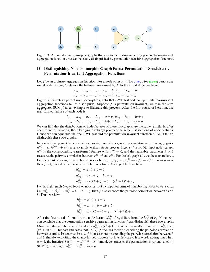
Figure 3: A pair of non-isomorphic graphs that cannot be distinguished by permutation-invariantaggregation functions, but can be easily distinguished by permutation-sensitive aggregation functions.

D Distinguishing Non-Isomorphic Graph Pairs: Permutation-Sensitive vs.Permutation-Invariant Aggregation Functions

Let f be an arbitrary aggregation function. For a node v, let xv (b for blue, g for green) denote theinitial node feature, hv denote the feature transformed by f . In the initial stage, we have:

xu1= xu2

= xu5= xu6

= b, xu3= xu4

= g

xv1 = xv2 = xv5 = xv6 = b, xv3 = xv4 = g

Figure 3 illustrates a pair of non-isomorphic graphs that 2-WL test and most permutation-invariantaggregation functions fail to distinguish. Suppose f is permutation-invariant, we take the sumaggregator SUM(·) as an example to illustrate this process. After the first round of iteration, thetransformed feature of each node is:

hu1 = hu2 = hu5 = hu6 = b+ g, hu3 = hu4 = 2b+ g

hv1 = hv2 = hv5 = hv6 = b+ g, hv3 = hv4 = 2b+ g

We can find that the distributions of node features of these two graphs are the same. Similarly, aftereach round of iteration, these two graphs always produce the same distributions of node features.Hence we can conclude that the 2-WL test and the permutation-invariant function SUM(·) fail todistinguish these two graphs.

In contrast, suppose f is permutation-sensitive, we take a generic permutation-sensitive aggregatorh(t) = k ·h(t−1) +x(t) as an example to illustrate its process. Here x(t) is the t-th input node feature,h(t) is the corresponding transformed feature with h(0) = 0, and the learnable parameter k > 1measures the pairwise correlation between x(t−1) and x(t). For the left graphG1, we focus on node u3.Let the input ordering of neighboring nodes be u1, u4, u5, i.e., x(1)u3 → x

(2)u3 → x

(3)u3 = b→ g → b,

then f only encodes the pairwise correlation between b and g. Thus, we have

h(1)u3= k · 0 + b = b

h(2)u3= k · b+ g = kb+ g

h(3)u3= k · (kb+ g) + b = (k2 + 1)b+ kg

For the right graphG2, we focus on node v3. Let the input ordering of neighboring nodes be v1, v2, v4,i.e., x(1)v3 → x

(2)v3 → x

(3)v3 = b→ b→ g, then f also encodes the pairwise correlation between b and

b. Thus, we haveh(1)v3 = k · 0 + b = b

h(2)v3 = k · b+ b = kb+ b

h(3)v3 = k · (kb+ b) + g = (k2 + k)b+ g

After the first round of iteration, the node feature h(3)u3 of u3 differs from the h(3)v3 of v3. Hence wecan conclude that the permutation-sensitive aggregation function f can distinguish these two graphs.Moreover, the weight ratio of b and g in h(3)u3 is (k2 + 1) : k, which is smaller than that in h(3)v3 , i.e.,(k2 + k) : 1. This fact indicates that, in G1, f focuses more on encoding the pairwise correlationbetween b and g. In contrast, in G2, f focuses more on encoding the pairwise correlation between band b, thereby exploiting the triangular substructure such as4v1v3v2. It is worth noting that whenk = 1, the function f is h(t) = h(t−1) + x(t) and degenerates to the permutation-invariant functionSUM(·), resulting in h(3)u3 = h

(3)v3 = 2b+ g.

17

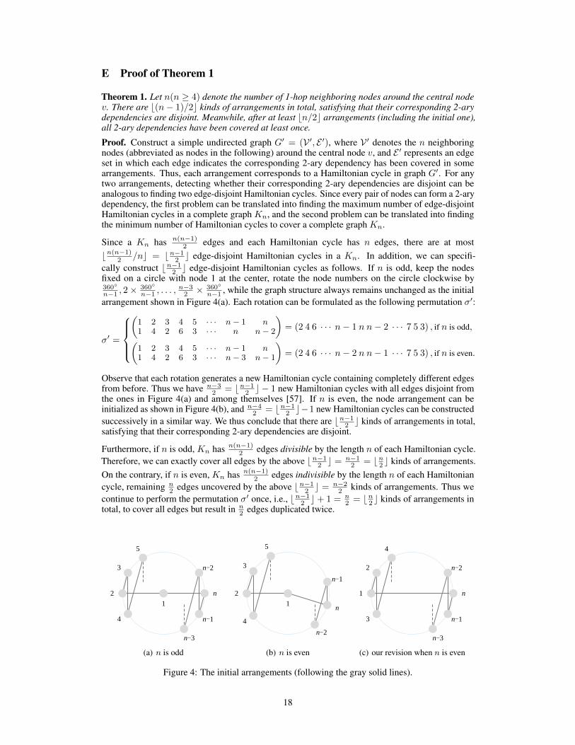
E Proof of Theorem 1

Theorem 1. Let n(n ≥ 4) denote the number of 1-hop neighboring nodes around the central nodev. There are b(n− 1)/2c kinds of arrangements in total, satisfying that their corresponding 2-arydependencies are disjoint. Meanwhile, after at least bn/2c arrangements (including the initial one),all 2-ary dependencies have been covered at least once.

Proof. Construct a simple undirected graph G′ = (V ′, E ′), where V ′ denotes the n neighboringnodes (abbreviated as nodes in the following) around the central node v, and E ′ represents an edgeset in which each edge indicates the corresponding 2-ary dependency has been covered in somearrangements. Thus, each arrangement corresponds to a Hamiltonian cycle in graph G′. For anytwo arrangements, detecting whether their corresponding 2-ary dependencies are disjoint can beanalogous to finding two edge-disjoint Hamiltonian cycles. Since every pair of nodes can form a 2-arydependency, the first problem can be translated into finding the maximum number of edge-disjointHamiltonian cycles in a complete graph Kn, and the second problem can be translated into findingthe minimum number of Hamiltonian cycles to cover a complete graph Kn.

Since a Kn has n(n−1)2 edges and each Hamiltonian cycle has n edges, there are at most

bn(n−1)2 /nc = bn−12 c edge-disjoint Hamiltonian cycles in a Kn. In addition, we can specifi-cally construct bn−12 c edge-disjoint Hamiltonian cycles as follows. If n is odd, keep the nodesfixed on a circle with node 1 at the center, rotate the node numbers on the circle clockwise by360

n−1 , 2×360

n−1 , . . . ,n−32 ×

360

n−1 , while the graph structure always remains unchanged as the initialarrangement shown in Figure 4(a). Each rotation can be formulated as the following permutation σ′:

σ′ =

(

1 2 3 4 5 · · · n− 1 n1 4 2 6 3 · · · n n− 2

)= (2 4 6 · · · n− 1 n n− 2 · · · 7 5 3) , if n is odd,(

1 2 3 4 5 · · · n− 1 n1 4 2 6 3 · · · n− 3 n− 1

)= (2 4 6 · · · n− 2 n n− 1 · · · 7 5 3) , if n is even.

Observe that each rotation generates a new Hamiltonian cycle containing completely different edgesfrom before. Thus we have n−3

2 = bn−12 c − 1 new Hamiltonian cycles with all edges disjoint fromthe ones in Figure 4(a) and among themselves [57]. If n is even, the node arrangement can beinitialized as shown in Figure 4(b), and n−4

2 = bn−12 c−1 new Hamiltonian cycles can be constructedsuccessively in a similar way. We thus conclude that there are bn−12 c kinds of arrangements in total,satisfying that their corresponding 2-ary dependencies are disjoint.

Furthermore, if n is odd, Kn has n(n−1)2 edges divisible by the length n of each Hamiltonian cycle.

Therefore, we can exactly cover all edges by the above bn−12 c = n−12 = bn2 c kinds of arrangements.

On the contrary, if n is even, Kn has n(n−1)2 edges indivisible by the length n of each Hamiltonian

cycle, remaining n2 edges uncovered by the above bn−12 c = n−2

2 kinds of arrangements. Thus wecontinue to perform the permutation σ′ once, i.e., bn−12 c+ 1 = n

2 = bn2 c kinds of arrangements intotal, to cover all edges but result in n

2 edges duplicated twice.

1

2

4

3

5

n

n-2

n-1

n-3

(a) n is odd

1

2

4

3

5

n-1

n

n-2

(b) n is even

1

3

2

4

n

n-2

n-1

n-3

(c) our revision when n is even

Figure 4: The initial arrangements (following the gray solid lines).

18

As discussed in the main body, these bn2 c arrangements and the corresponding bn2 c Hamiltoniancycles are modeled by the permutation-sensitive function in a directed manner. In addition, wealso expect to reverse these bn2 c directed Hamiltonian cycles by performing the permutation σ′

successively, thereby transforming them into an undirected manner. However, σ′ cannot satisfy thisrequirement if n is even. Thus, we propose to revise the permutation σ′ into the following one:

σ =

(

1 2 3 4 5 · · · n− 1 n1 4 2 6 3 · · · n n− 2

)= (2 4 6 · · · n− 1 n n− 2 · · · 7 5 3) , if n is odd,(

1 2 3 4 · · · n− 1 n3 1 5 2 · · · n n− 2

)= (1 3 5 · · · n− 1 n n− 2 · · · 6 4 2) , if n is even.

where σ is the same as σ′ when n is odd, but a little different when n is even. If n is even, σ isan n-cycle, but σ′ is an (n − 1)-cycle. The corresponding initial node arrangement after revisionis shown in Figure 4(c). After adding a virtual node 0 at the center in Figure 4(c), σ becomes thesame as σ′ with n + 1 in Figure 4(a), which can cover all edges with b (n+1)−1

2 c = bn2 c kinds ofarrangements. Moreover, after performing σ for n times in succession, it can cover a complete graphbi-directionally but σ′ fails.

In conclusion, after performing σ or σ′ for bn2 c − 1 times in succession (excluding the initial one),all 2-ary dependencies have been covered at least once.

F Proof of Lemma 2

Theorem F.1. The order of any permutation is the least common multiple of the lengths of its disjointcycles [54].Proposition F.2. The order of a cyclic group is equal to the order of its generator [53].

Using Theorem F.1 and Proposition F.2, we prove Lemma 2 as follows.

Lemma 2. For the permutation σ of n indices, G = e, σ, σ2, . . . , σn−2 is a permutation groupisomorphic to the cyclic group Zn−1 if n is odd. And G = e, σ, σ2, . . . , σn−1 is a permutationgroup isomorphic to the cyclic group Zn if n is even.Proof. If n is odd, we find the order of permutation σ first. Since

σ =

(1 2 3 4 5 · · · n− 1 n1 4 2 6 3 · · · n n− 2

)= (1) (2 4 6 · · · n− 1 n n− 2 · · · 7 5 3)

Let π1 = (1), π2 = (2 4 6 · · · n− 1 n n− 2 · · · 7 5 3), then the permutation σ can be representedas the product of these two disjoint cycles, i.e., σ = π1π2. Here π1 is a 1-cycle of length 1, π2is an (n − 1)-cycle of length n − 1. Using Theorem F.1, the order of permutation σ is the leastcommon multiple of 1 and n− 1: lcm(1, n− 1) = n− 1, which indicates that σn−1 = e. Therefore,G = e, σ, σ2, . . . , σn−2 is a permutation group generated by σ, i.e., G = 〈σ〉. Accordingto the definition of the cyclic group (see Appendix B), G is isomorphic to a cyclic group. ByProposition F.2, the order of group G = 〈σ〉 is equal to the order of its generator σ, i.e., n− 1. Thus,G = e, σ, σ2, . . . , σn−2 is a permutation group isomorphic to the cyclic group Zn−1.

Similarly, we can prove that G = e, σ, σ2, . . . , σn−1 is a permutation group isomorphic to thecyclic group Zn if n is even.

Theorem F.3 (Cayley’s Theorem). Every finite group is isomorphic to a permutation group [53].

The conclusion of Lemma 2 also obeys the most fundamental Cayley’s Theorem in group theory.

G Proof of Corollary 3 and the Diagram of Group Action

Corollary 3. The map α : G× S → S denoted by (g, s) 7→ gs is a group action of G on S.Proof. Let e be the identity element of G and idσ be the identity permutation. And let denote thecomposition in G. For all σi, σj ∈ G and s ∈ S, we have

α(e, s) = e · s = idσ · s = s

α(σiσj , s) = (σi σj) · s = σi · (σj · s) = α(σi, α(σj , s))

Thus, the map α defines a group action of the permutation group G on the set S.

19

1

27

6 3

45

1

27

6 3

45

1

27

6 3

45

1

27

6 3

45

1 2 3 4 5 6 7

1 7 6 5 4 3 2

=1 2 3 4 5 6 7

1 4 2 6 3 7 5

1

27

36

45

1

27

36

45

e

σ

σ2

σ3

σ4

σ5

(a) G1 = e, σ, σ2, . . . , σ5 ∼= Z6

1

2

3

4

5

6

7

8

1

2

3

4

5

6

7

8

1

2

3

4

5

6

7

8

1

2

3

4

5

6

7

8

1

2

3

4

5

6

7

8

1

2

3

4

5

6

7

8

1

2

3

4

5

6

7

8

1

2

3

4

5

6

7

8

1

2

3

4

5

6

7

8

1 2 3 4 5 6 7 8

8 7 6 5 4 3 2 1

4

6 2

8

1 7

3

5

5

3 7

1

8 2

6

4

=1 2 3 4 5 6 7 8

3 1 5 2 7 4 8 6σ

2

e

σ

σ3

σ4

σ5

σ6

σ7

(b) G2 = e, σ, σ2, . . . , σ7 ∼= Z8

Figure 5: The group structure of the permutation group G and the results of its actions on the set S.

20

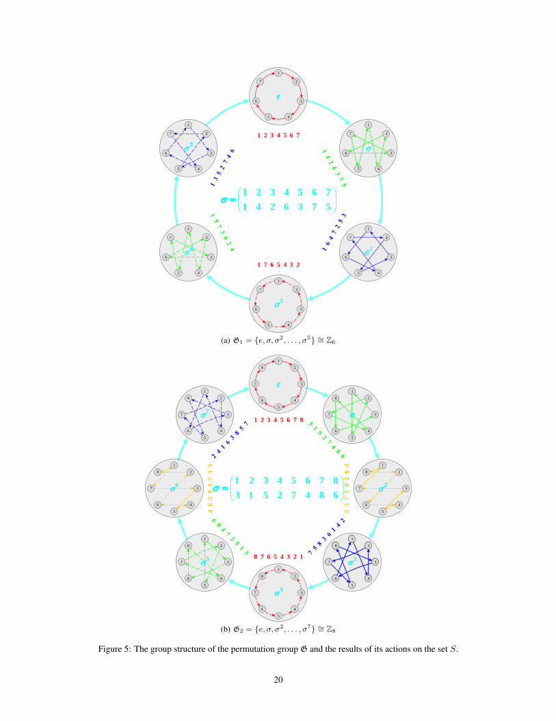
To better understand Lemma 2 and Corollary 3, we provide diagrams to illustrate the group actionsof the permutation groups G1 = e, σ, σ2, . . . , σ5 and G2 = e, σ, σ2, . . . , σ7 when n = 7 andn = 8, respectively. As shown in Figures 5(a) and 5(b), the overall frameworks with big light-gray circles and cyan arrows represent the Cayley diagrams of the permutation groups G1

∼= Z6

and G2∼= Z8 constructed by Lemma 2, respectively. The center of each subfigure presents the

corresponding generator σ. Each big light-gray circle represents an element g (i.e., a permutation) ofgroup G, marked at the center of the circle. And each cyan arrow gi → gj indicates the relationshipgj = gi σ exists between two group elements gi, gj ∈ G. After g acts on the elements 1, . . . , n ofthe set S, the corresponding images are presented as the colored numbers next to the big light-graycircle. Finally, the 2-ary dependencies (colored arrows) between neighboring nodes (small dark-graycircles) are modeled according to the action results of g, shown in each big light-gray circle.

H Proofs About Incidence Triangles

H.1 Proof of Eq. (6)

τ =1

2A2 A · 1N , 1>Nτ =

1

2tr(A3)

Proof. LetA = (aij)N×N ,B = A2 = (bij)N×N , where aij and bij denote the (i, j) element ofAandB, respectively. Since aij equals 1 iff nodes vi and vj are adjacent in G, bij equals the numberof walks of length 2 from nodes vi to vj in G. In addition, a walk of length 2 from vi to vj and anedge from vj to vi form a triangle containing both vi and vj . Therefore, the (i, j) element ofA2Aequals bijaij = bijaji, which indicates how many triangles contain both vi and vj . We can use a sumvector 1N = (1, 1, · · · , 1)> ∈ RN to sum up each row of A2 A and get a result vector, whosei-th element gives twice the number of incidence triangles of node vi. Here the “twice” comes fromthe fact that each incidence triangle4vjvivk over node vi has two walks of length 2 starting fromnode vi, that is, vi → vj → vk and vi → vk → vj . Hence after dividing each element of the resultvector by 2, we finally obtain τ = 1

2A2 A · 1N .

For the second equation, we have

1>Nτ =1

21>N · (A2A) ·1N =

1

2

N∑i=1

N∑j=1

bijaij =1

2

N∑i=1

(A2 ·A>)ii =1

2tr(A2 ·A>) =

1

2tr(A3)

Remark. The i-th diagonal entry ofA3 is equal to twice the number of triangles in which the i-thnode is contained [41]. In addition, each triangle has three vertices. Hence we can divide the sum ofthe diagonal entries by 6 to obtain the total number of triangles in graph G, i.e., 1

6 tr(A3) [58].

For directed graphs, we also have similar results:

~τ = A2 A> · 1N , 1>N~τ = tr(A3)

where ~τ ∈ RN and its i-th element ~τi denotes the number of directed incidence triangles over node i.

H.2 Proof of Theorem 4

Theorem H.1 (Chernoff-Hoeffding Bound for Discrete Time Markov Chain [59]). Let M bean ergodic Markov chain with state space [n] = 1, 2, . . . , n and stationary distribution π. Lett = t(ε) be its ε-mixing time for ε ≤ 1/8. Let (X1, X2, . . . , Xr) denote an r-step random walk onMstarting from an initial distribution ϕ on [n], i.e., X1 ← ϕ. Define ‖ϕ‖π =

∑ni=1

ϕ2i

πi. For every step

k ∈ [r], let f (k) : [n]→ [0, 1] be a weight function such that the expectation EXk←π[f (k)(Xk)] = µ

for all k. Define the total weight of the walk (X1, X2, . . . , Xr) by Z ,∑rk=1 f(Xk). There exists

some constant c (which is independent of µ, δ and ε) such that for 0 < δ < 1

Pr (|Z − µr| > εµr) ≤ c ‖ϕ‖π exp

(−ε

2µr

72t

)or equivalently

Pr

(∣∣∣∣Zr − µ∣∣∣∣ > εµ

)≤ c ‖ϕ‖π exp

(−ε

2µr

72t

).

21

Theorem H.2. Any nonlinear dynamic system may be approximated by a recurrent neural networkto any desired degree of accuracy and with no restrictions imposed on the compactness of the statespace, provided that the network is equipped with an adequate number of hidden neurons [60].

Using Theorem H.1 and Theorem H.2, we prove Theorem 4 as follows.

Theorem 4. Let xv,∀v ∈ V denote the feature inputs on graph G = (V, E), and M be a generalGNN model with RNN aggregators. Suppose that xv is initialized as the degree dv of node v, andeach node is distinguishable. For any 0 < ε ≤ 1/8 and 0 < δ < 1, there exists a parameter setting

Θ for M so that after O(dv(2dv+τv)t

dv+τv

)samples,

Pr

(∣∣∣∣zvτv − 1

∣∣∣∣ ≤ ε) ≥ 1− δ, ∀v ∈ V,

where zv ∈ R is the final output value generated by M and τv is the number of incidence triangles.Proof. Without loss of generality, we discuss how to estimate the number of incidence trianglesτ0 for an arbitrary node v0 based on its n neighbors v′1, v

′2, . . . , v

′n. Let v′0 = v0, and let G′ =

(V ′, E ′) denote the subgraph induced by V ′ = v′0, v′1, v′2, . . . , v′n, with an adjacency matrixA′ ∈R(n+1)×(n+1). We add a symbol “′” to all notations of the induced subgraph G′ to distinguish themfrom those of graph G. For each node v′i ∈ V ′, d′i denotes the degree of v′i in graph G′, τ ′i denotesthe number of incidence triangles of v′i in graph G′. In particular, d′0 = d0 = n, τ ′0 = τ0. Our goal isto estimate τ0 for an arbitrary node v0 in graph G, which is equal to τ ′0 in graph G′.

A simple random walk (SRW) with r steps on graph G′, denoted by R = (X1, X2, . . . , Xr), isdefined as follows: start from an initial node in G′, then move to one of its neighboring nodes chosenuniformly at random, and repeat this process (r − 1) times. This random walk on graph G′ can beviewed as a finite Markov chainM with the state space V ′, and the transition probability matrix Pof this Markov chain is defined as

P (i, j) =

1

d′i, if (v′i, v

′j) ∈ E ′,

0, otherwise.

Let D′ =∑ni=0 d

′i = 2 |E ′| denote the sum of degrees in graph G′. After many random walk steps,

the probability Pr(Xr = v′i) converges to pi , d′i/D′, and the vector π = (p0, p1, . . . , pn) is called

the stationary distribution of this random walk.

The mixing time of a Markov chain is the number of steps it takes for a random walk to approachits stationary distribution. We adopt the definition in [41, 59, 61] and define the mixing time t(ε) asfollows:

t(ε) = maxXi∈V′

mint :∣∣∣π − π(i)P t

∣∣∣ < ε

where π is the stationary distribution of the Markov chain defined above, π(i) is the initial distributionwhen starting from state Xi ∈ V ′, P t is the transition matrix after t steps, and | · | is the variationdistance between two distributions.

Later on, we will exploit node samples taken from a random walk to construct an estimator z0, thenuse the mixing time based Chernoff-Hoeffding bound [59] to compute the number of steps/samplesneeded, thereby guaranteeing that our estimator z0 is within (1 ± ε) of the true value τ0 with theprobability of at least 1− δ.

Given a random walk (X1, X2, . . . , Xr) on graph G′, we define a new variable ak = A′Xk−1,Xk+1

for every 2 ≤ k ≤ r − 1, then we have

E[akd′Xk

]=

n∑i=0

piE[akd′Xk

∣∣ Xk = v′i]

=

n∑i=0

d′iD′

2τ ′id′i

2 d′i

=2

D′

n∑i=0

τ ′i (7)

22

The second equality holds because there are d′i2 equal probability combinations of (Xk−1, v

′i, Xk+1),

out of which only 2τ ′i combinations form a triangle (u′, v′i, w′) or its reverse (w′, v′i, u

′), where u′ isconnected to w′, i.e., ak = A′Xk−1,Xk+1

= A′u′,w′ = 1.

To estimate τ0, we introduce two variables Y1 and Y2, defined as follows:

Y1 ,1

r − 2

r−1∑k=2

akd′Xk, Y2 ,

1

r

r∑k=1

1

d′Xk

Using the linearity of expectation and Eq. (7), we obtain

E[Y1] =1

r − 2

r−1∑k=2

E[akd′Xk

]=

2

D′

n∑i=0

τ ′i (8)

Similarly, we have

E[Y2] =1

r

r∑k=1

E

[1

d′Xk

]=

1

r

r∑k=1

(n∑i=0

d′iD′

1

d′i

)=n+ 1

D′(9)

Recall that G′ is a subgraph induced by V ′ = v′0, v′1, v′2, . . . , v′n, where v′1, v′2, . . . , v

′n are n

neighbors of an arbitrary node v′0 = v0. Therefore, the maximum degree of graph G′ is ∆′ = n,which is equal to d′0 = d0. In addition, we have

∑ni=0 τ

′i = 3τ ′0 = 3τ0, and D′ = 2 |E ′| =

2(d′0 + τ ′0) = 2(d0 + τ0). Substituting them in Eq. (8) and Eq. (9), we get

E[Y1] =3τ0

d0 + τ0(10)

andE[Y2] =

d0 + 1

2(d0 + τ0)(11)

From Eq. (10) and Eq. (11) we can isolate τ0 and get

τ0 =d0 + 1

6· E[Y1]

E[Y2](12)

Since d0 is the feature input, the coefficientd0 + 1

6can be considered as a constant factor here.

Intuitively, both Y1 and Y2 converge to their expected values, and thus the estimator z0 ,d0 + 1

6· Y1Y2

converges to τ0 as well. Next, we will find the number of steps/samples r for convergence.

Since akd′Xk= A′Xk−1,Xk+1

d′Xkin Y1 only depends on a 3-nodes history, we observe a related

Markov chain M that remembers the three latest visited nodes. Accordingly, M has (n + 1) ×(n + 1) × (n + 1) states, and (Xk−1, Xk, Xk+1) → (Xk, Xk+1, Xk+2) has the same transitionprobability as Xk+1 → Xk+2 inM. Define each state Xk = (Xk−1, Xk, Xk+1) for 2 ≤ k ≤ r − 1.

Let f (k)1 (Xk) = f(k)1 (Xk) =

akd′Xk

∆′=

akd′Xk

d0such that all values of f (k)1 (Xk) are in [0, 1].

By Eq. (7), Eq. (8), and Eq. (10), we have µ1 = EXk←π(f(k)1 (Xk)) =

3τ0d0(d0 + τ0)

. Define

Z1 ,r−1∑k=2

f(k)1 (Xk) =

r − 2

d0Y1, assume that ϕ ≈ π thus ‖ϕ‖π = 1. By Theorem H.1 and Eq. (10),

we have

Pr(|Y1 − E[Y1]| > ε

3E[Y1]

)≤ c1 exp

(− 3 · ε2τ0(r − 2)

9 · 72 · td0(d0 + τ0)

)(13)

Extracting rY1from

δ

2= c1 exp

(− ε2τ0(r − 2)

216 · td0(d0 + τ0)

), we obtain rY1

= 2 − 216ln(δ/2c1)

ε2·

d0(d0 + τ0)t

τ0= O

(d0(d0 + τ0)t

τ0

), where c1, ε and δ are all constants.

23

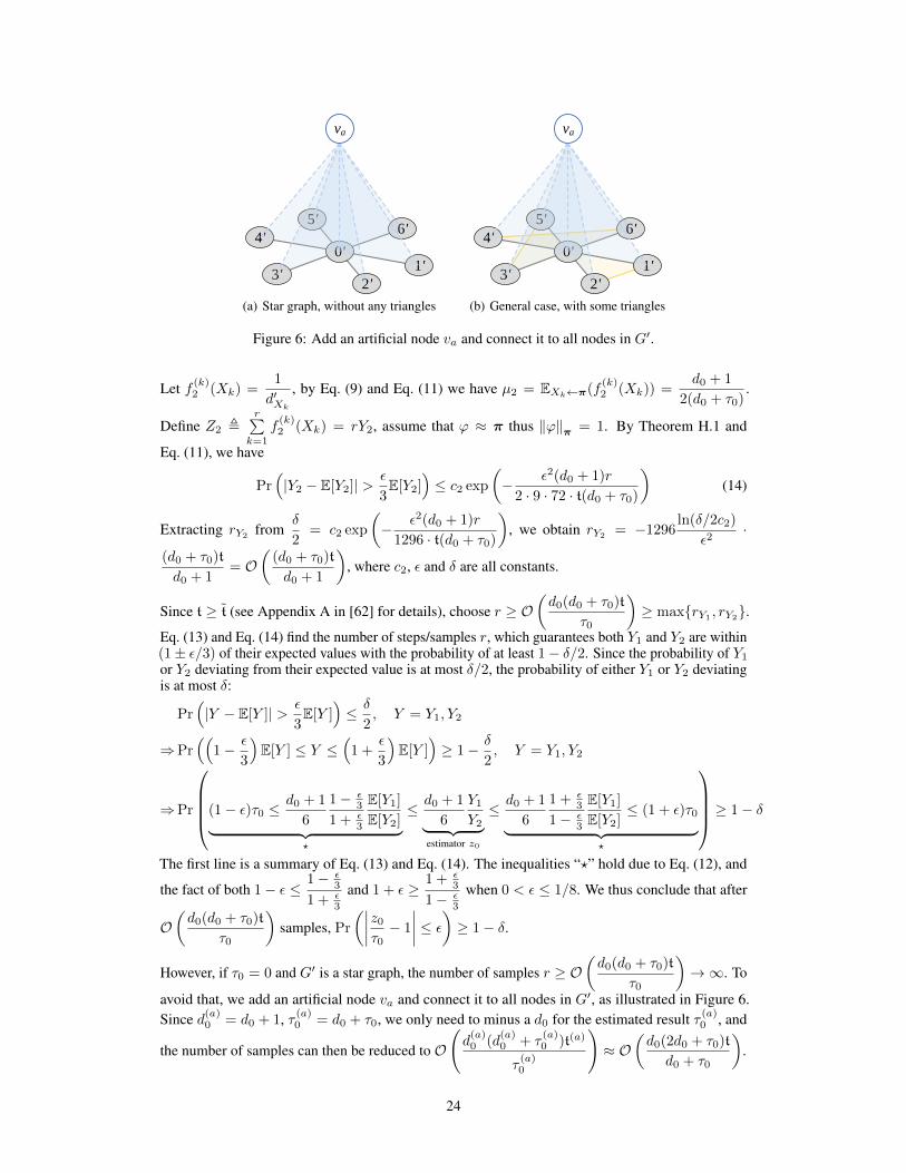
1'

2'3'

6'5'

4'0'

va

(a) Star graph, without any triangles

1'

2'3'

6'5'

4'0'

va

(b) General case, with some triangles

Figure 6: Add an artificial node va and connect it to all nodes in G′.

Let f (k)2 (Xk) =1

d′Xk

, by Eq. (9) and Eq. (11) we have µ2 = EXk←π(f(k)2 (Xk)) =

d0 + 1

2(d0 + τ0).

Define Z2 ,r∑

k=1

f(k)2 (Xk) = rY2, assume that ϕ ≈ π thus ‖ϕ‖π = 1. By Theorem H.1 and

Eq. (11), we have

Pr(|Y2 − E[Y2]| > ε

3E[Y2]

)≤ c2 exp

(− ε2(d0 + 1)r

2 · 9 · 72 · t(d0 + τ0)

)(14)

Extracting rY2from

δ

2= c2 exp

(− ε2(d0 + 1)r

1296 · t(d0 + τ0)

), we obtain rY2

= −1296ln(δ/2c2)

ε2·

(d0 + τ0)t

d0 + 1= O

((d0 + τ0)t

d0 + 1

), where c2, ε and δ are all constants.

Since t ≥ t (see Appendix A in [62] for details), choose r ≥ O(d0(d0 + τ0)t

τ0

)≥ maxrY1

, rY2.

Eq. (13) and Eq. (14) find the number of steps/samples r, which guarantees both Y1 and Y2 are within(1± ε/3) of their expected values with the probability of at least 1− δ/2. Since the probability of Y1or Y2 deviating from their expected value is at most δ/2, the probability of either Y1 or Y2 deviatingis at most δ:

Pr(|Y − E[Y ]| > ε

3E[Y ]

)≤ δ

2, Y = Y1, Y2

⇒Pr((

1− ε

3

)E[Y ] ≤ Y ≤

(1 +

ε

3

)E[Y ]

)≥ 1− δ

2, Y = Y1, Y2

⇒Pr

(1− ε)τ0 ≤d0 + 1

6

1− ε3

1 + ε3

E[Y1]

E[Y2]︸ ︷︷ ︸?

≤ d0 + 1

6

Y1Y2︸ ︷︷ ︸

estimator z0

≤ d0 + 1

6

1 + ε3

1− ε3

E[Y1]

E[Y2]≤ (1 + ε)τ0︸ ︷︷ ︸

?

≥ 1− δ

The first line is a summary of Eq. (13) and Eq. (14). The inequalities “?” hold due to Eq. (12), and

the fact of both 1− ε ≤1− ε

3

1 + ε3

and 1 + ε ≥1 + ε

3

1− ε3

when 0 < ε ≤ 1/8. We thus conclude that after

O(d0(d0 + τ0)t

τ0

)samples, Pr

(∣∣∣∣z0τ0 − 1

∣∣∣∣ ≤ ε) ≥ 1− δ.

However, if τ0 = 0 and G′ is a star graph, the number of samples r ≥ O(d0(d0 + τ0)t

τ0

)→∞. To

avoid that, we add an artificial node va and connect it to all nodes in G′, as illustrated in Figure 6.Since d(a)0 = d0 + 1, τ (a)0 = d0 + τ0, we only need to minus a d0 for the estimated result τ (a)0 , and

the number of samples can then be reduced to O

(d(a)0 (d

(a)0 + τ

(a)0 )t(a)

τ(a)0

)≈ O

(d0(2d0 + τ0)t

d0 + τ0

).

24

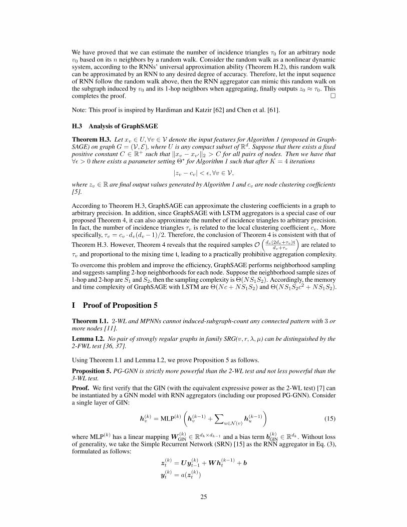
We have proved that we can estimate the number of incidence triangles τ0 for an arbitrary nodev0 based on its n neighbors by a random walk. Consider the random walk as a nonlinear dynamicsystem, according to the RNNs’ universal approximation ability (Theorem H.2), this random walkcan be approximated by an RNN to any desired degree of accuracy. Therefore, let the input sequenceof RNN follow the random walk above, then the RNN aggregator can mimic this random walk onthe subgraph induced by v0 and its 1-hop neighbors when aggregating, finally outputs z0 ≈ τ0. Thiscompletes the proof.

Note: This proof is inspired by Hardiman and Katzir [62] and Chen et al. [61].

H.3 Analysis of GraphSAGE

Theorem H.3. Let xv ∈ U,∀v ∈ V denote the input features for Algorithm 1 (proposed in Graph-SAGE) on graph G = (V, E), where U is any compact subset of Rd. Suppose that there exists a fixedpositive constant C ∈ R+ such that ‖xv − xv′‖2 > C for all pairs of nodes. Then we have that∀ε > 0 there exists a parameter setting Θ∗ for Algorithm 1 such that after K = 4 iterations

|zv − cv| < ε,∀v ∈ V,

where zv ∈ R are final output values generated by Algorithm 1 and cv are node clustering coefficients[5].

According to Theorem H.3, GraphSAGE can approximate the clustering coefficients in a graph toarbitrary precision. In addition, since GraphSAGE with LSTM aggregators is a special case of ourproposed Theorem 4, it can also approximate the number of incidence triangles to arbitrary precision.In fact, the number of incidence triangles τv is related to the local clustering coefficient cv. Morespecifically, τv = cv ·dv(dv−1)/2. Therefore, the conclusion of Theorem 4 is consistent with that ofTheorem H.3. However, Theorem 4 reveals that the required samples O

(dv(2dv+τv)t

dv+τv

)are related to

τv and proportional to the mixing time t, leading to a practically prohibitive aggregation complexity.

To overcome this problem and improve the efficiency, GraphSAGE performs neighborhood samplingand suggests sampling 2-hop neighborhoods for each node. Suppose the neighborhood sample sizes of1-hop and 2-hop are S1 and S2, then the sampling complexity is Θ(NS1S2). Accordingly, the memoryand time complexity of GraphSAGE with LSTM are Θ(Nc+NS1S2) and Θ(NS1S2c

2 +NS1S2).

I Proof of Proposition 5

Theorem I.1. 2-WL and MPNNs cannot induced-subgraph-count any connected pattern with 3 ormore nodes [11].

Lemma I.2. No pair of strongly regular graphs in family SRG(v, r, λ, µ) can be distinguished by the2-FWL test [36, 37].

Using Theorem I.1 and Lemma I.2, we prove Proposition 5 as follows.

Proposition 5. PG-GNN is strictly more powerful than the 2-WL test and not less powerful than the3-WL test.Proof. We first verify that the GIN (with the equivalent expressive power as the 2-WL test) [7] canbe instantiated by a GNN model with RNN aggregators (including our proposed PG-GNN). Considera single layer of GIN:

h(k)v = MLP(k)

(h(k−1)v +

∑u∈N (v)

h(k−1)u

)(15)

where MLP(k) has a linear mapping W (k)GIN ∈ Rdk×dk−1 and a bias term b

(k)GIN ∈ Rdk . Without loss

of generality, we take the Simple Recurrent Network (SRN) [15] as the RNN aggregator in Eq. (3),formulated as follows:

z(k)t = Uy

(k)t−1 +Wh

(k−1)t + b

y(k)t = a(z

(k)t )

25

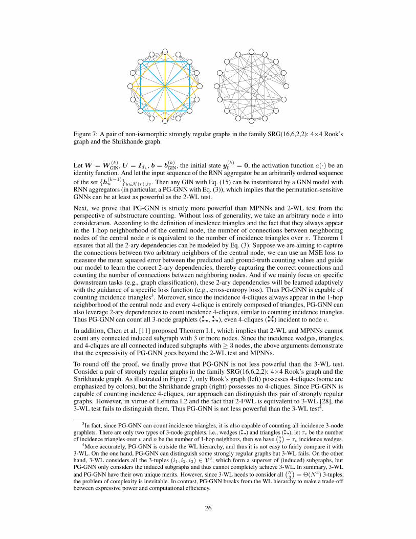
Figure 7: A pair of non-isomorphic strongly regular graphs in the family SRG(16,6,2,2): 4×4 Rook’sgraph and the Shrikhande graph.

Let W = W(k)GIN, U = Idk , b = b

(k)GIN, the initial state y(k)

0 = 0, the activation function a(·) be anidentity function. And let the input sequence of the RNN aggregator be an arbitrarily ordered sequenceof the set h(k−1)

u u∈N (v)∪v . Then any GIN with Eq. (15) can be instantiated by a GNN model withRNN aggregators (in particular, a PG-GNN with Eq. (3)), which implies that the permutation-sensitiveGNNs can be at least as powerful as the 2-WL test.

Next, we prove that PG-GNN is strictly more powerful than MPNNs and 2-WL test from theperspective of substructure counting. Without loss of generality, we take an arbitrary node v intoconsideration. According to the definition of incidence triangles and the fact that they always appearin the 1-hop neighborhood of the central node, the number of connections between neighboringnodes of the central node v is equivalent to the number of incidence triangles over v. Theorem 1ensures that all the 2-ary dependencies can be modeled by Eq. (3). Suppose we are aiming to capturethe connections between two arbitrary neighbors of the central node, we can use an MSE loss tomeasure the mean squared error between the predicted and ground-truth counting values and guideour model to learn the correct 2-ary dependencies, thereby capturing the correct connections andcounting the number of connections between neighboring nodes. And if we mainly focus on specificdownstream tasks (e.g., graph classification), these 2-ary dependencies will be learned adaptivelywith the guidance of a specific loss function (e.g., cross-entropy loss). Thus PG-GNN is capable ofcounting incidence triangles3. Moreover, since the incidence 4-cliques always appear in the 1-hopneighborhood of the central node and every 4-clique is entirely composed of triangles, PG-GNN canalso leverage 2-ary dependencies to count incidence 4-cliques, similar to counting incidence triangles.Thus PG-GNN can count all 3-node graphlets ( , ), even 4-cliques ( ) incident to node v.

In addition, Chen et al. [11] proposed Theorem I.1, which implies that 2-WL and MPNNs cannotcount any connected induced subgraph with 3 or more nodes. Since the incidence wedges, triangles,and 4-cliques are all connected induced subgraphs with ≥ 3 nodes, the above arguments demonstratethat the expressivity of PG-GNN goes beyond the 2-WL test and MPNNs.

To round off the proof, we finally prove that PG-GNN is not less powerful than the 3-WL test.Consider a pair of strongly regular graphs in the family SRG(16,6,2,2): 4×4 Rook’s graph and theShrikhande graph. As illustrated in Figure 7, only Rook’s graph (left) possesses 4-cliques (some areemphasized by colors), but the Shrikhande graph (right) possesses no 4-cliques. Since PG-GNN iscapable of counting incidence 4-cliques, our approach can distinguish this pair of strongly regulargraphs. However, in virtue of Lemma I.2 and the fact that 2-FWL is equivalent to 3-WL [28], the3-WL test fails to distinguish them. Thus PG-GNN is not less powerful than the 3-WL test4.

3In fact, since PG-GNN can count incidence triangles, it is also capable of counting all incidence 3-nodegraphlets. There are only two types of 3-node graphlets, i.e., wedges ( ) and triangles ( ), let τv be the numberof incidence triangles over v and n be the number of 1-hop neighbors, then we have

(n2

)− τv incidence wedges.

4More accurately, PG-GNN is outside the WL hierarchy, and thus it is not easy to fairly compare it with3-WL. On the one hand, PG-GNN can distinguish some strongly regular graphs but 3-WL fails. On the otherhand, 3-WL considers all the 3-tuples (i1, i2, i3) ∈ V3, which form a superset of (induced) subgraphs, butPG-GNN only considers the induced subgraphs and thus cannot completely achieve 3-WL. In summary, 3-WLand PG-GNN have their own unique merits. However, since 3-WL needs to consider all

(N3

)= Θ(N3) 3-tuples,

the problem of complexity is inevitable. In contrast, PG-GNN breaks from the WL hierarchy to make a trade-offbetween expressive power and computational efficiency.

26

In conclusion, our proposed PG-GNN is strictly more powerful than the 2-WL test and not lesspowerful than the 3-WL test.

J Details of the Proposed Model

In this section, we discuss the proposed model in detail. The notations follow the definitions inSection 3.1, i.e., let n denote the number of 1-hop neighbors of the central node v. Suppose these nneighbors are randomly numbered as u1, . . . , un (also abbreviated as 1, . . . , n for simplicity), the setof neighboring nodes is represented as N (v) (or S = [n] = 1, . . . , n).

J.1 Illustration of the Proposed Model

Figure 8 presents a further explanation of Figure 2 and the relationships among Theorem 1, Lemma 2,Corollary 3, Figure 2, and Eq. (3). In this figure, we ignore the central node v for clarity and illustratefor n = 5 and n = 6. Here we take n = 5 as an example to explain Figure 8(a).

The very left column shows the components of Figure 2 and Eq. (3), and the right four columnsprovide the decoupled illustrations of Figure 2 and Eq. (3). The first row of the right four columnslists the group action gui (g acts on ui) defined by Corollary 3, where ui ranges from u1 to u5,g ∈ G = e, σ, σ2, σ3 and G is defined by Lemma 2. For readers unfamiliar with group theory,the third row of the right four columns explicitly provides the corresponding action results of gui,such as σ2u1 = u1, σ

2u2 = u5, σ2u3 = u4, σ

2u4 = u3, σ2u5 = u2 in the third column. In addition,

these four columns are associated with each other by the generator σ. For example, in the third row,after σ acts on the action results in the first column, they are transformed into the action results in thesecond column according to the permutation diagram, i.e., σu1 = u1, σu2 = u4, σu3 = u2, σu4 =u5, σu5 = u3. Action results in other columns are transformed in a similar manner and form a cyclicstructure. The second row of the right four columns illustrates this process.

In each column, after obtaining the action results of gu1, . . . , gun, we arrange these n = 5 neighbors(action results) as an undirected ring. The first bn/2c = 2 arrangements (marked by solid lines)are constructed according to Theorem 1, and the last bn/2c = 2 arrangements (marked by dashedlines) reverse the former. Either the first or the last bn/2c = 2 arrangements cover all undirected2-ary dependencies. Then, we use permutation-sensitive RNNs to model the 2-ary dependencies in adirected manner (since permutation-sensitive RNNs serve a→ b and b→ a as two different pairs)and construct the corresponding Hamiltonian cycles. As a result, the Hamiltonian cycles are modeledbi-directionally, and edges in Hamiltonian cycles are transformed into an undirected manner. Thearrangement generation and Hamiltonian cycle construction are detailed in Section 3.3.

Figure 8(b) presents in a similar way as Figure 8(a) does. However, we do not show all six columnsdue to the limited space. Here we omit the 5th and the 6th columns, which illustrate the modelingprocesses based on group elements σ4 and σ5.

J.2 Discussion on Groups

Since the (permutation) group in Eq. (3) plays a pivotal role in our model, it is necessary to discussthe motivation for using groups and why we select the specific group. In fact, the group is usedto effectively model all 2-ary dependencies (pairwise correlations). We first summarize why themodeling of all 2-ary dependencies is indispensable:

• Expressive power. Modeling all 2-ary dependencies can capture whether any two neighbor-ing nodes are connected, helping our model count incidence triangles and 4-cliques henceimproving its expressive power.

• Generalization capability and computational complexity. Modeling all 2-ary dependenciescan make these dependencies invariant to arbitrary permutations of node orderings. Suchan invariance to 2-ary dependencies is an approximation of the permutation-invariance andhelps to guarantee the generalization capability. Moreover, it also avoids considering all n!permutations to strictly ensure the permutation-invariance, thereby significantly reducingthe computational complexity.

• Robustness. Modeling all 2-ary dependencies makes our model insensitive to a specific2-ary dependency and robust to potential data noise and adversarial perturbations.

27

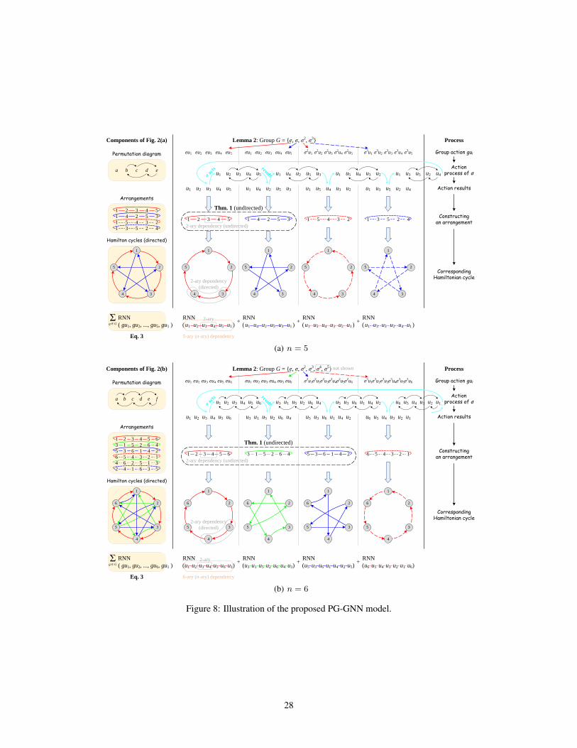
a b c d e

1 2 3 4 5

1 4 2 5 3

1 5 4 3 2

1 3 5 2 4

1

25

34

Permutation diagram

Σ( gu1, gu2, ..., gu5, gu1 )

g ∈ G

RNN

Eq. 3

Hamilton cycles (directed)

Arrangements

Components of Fig. 2(a)

1 2 3 4 5 1 4 2 5 3 1 5 4 3 2 1 3 5 2 4

1

25

34

1

25

34

1

25

34

1

25

34

Lemma 2: Group G = e, σ, σ2, σ3

u1 u2 u3 u4 u5 u1 u4 u2 u5 u3 u1 u5 u4 u3 u2 u1 u3 u5 u2 u4

RNN

eu1 eu2 eu3 eu4 eu5 σu1 σu2 σu3 σu4 σu5 σ2u1 σ2u2 σ

2u3 σ2u4 σ

2u5 σ3u1 σ3u2 σ

3u3 σ3u4 σ

3u5

u1 u2 u3 u4 u5 u1( ) u1 u4 u2 u5 u3 u1( )

RNN RNN

u1 u5 u4 u3 u2 u1( ) u1 u3 u5 u2 u4 u1( )

RNN

u1 u2 u3 u4 u5 u1 u4 u2 u5 u3 u1 u5 u4 u3 u2 u1 u3 u5 u2 u4

+ + +

2-ary dependency (undirected)

Thm. 1 (undirected)

2-ary

5-ary (n-ary) dependency

2-ary dependency

(directed)

Process

Group action gui

Action results

Constructingan arrangement

Corresponding Hamiltonian cycle

Actionprocess of σ

(a) n = 5

Process

Group action gui

Action results

Constructingan arrangement

Corresponding Hamiltonian cycle

Actionprocess of σ

Permutation diagram

Arrangements

Components of Fig. 2(b) Lemma 2: Group G = e, σ, σ2, σ3, σ4, σ5

eu1 eu2 eu3 eu4 eu5 σu1 σu2 σu3 σu4 σu5 σ2u1σ2u2σ

2u3σ2u4σ

2u5 σ3u1σ3u2σ

3u3σ3u4σ

3u5

a b c d e fu1 u2 u3 u4 u5 u6

u1 u2 u3 u4 u5 u6

1 2 3 4 5 6

3 1 5 2 6 4

5 3 6 1 4 2

6 5 4 3 2 1

4 6 2 5 1 3

2 4 1 6 3 5

Σ( gu1, gu2, ..., gu6, gu1 )

g ∈ G

RNN

Eq. 3

Hamilton cycles (directed)

RNN

( ) u3 u1 u3( )

RNN RNN RNN+ + +2-ary

6-ary (n-ary) dependency

2-ary dependency

(directed)

1

2

3

4

5

6

1

2

3

4

5

6

1

2

3

4

5

6

1

2

3

4

5

6

1

2

3

4

5

6

u3 u1 u5 u2 u6 u4 u5 u3 u6 u1 u4 u2 u6 u5 u4 u3 u2 u1

2-ary dependency (undirected)

Thm. 1 (undirected)

3 1 5 2 6 41 2 3 4 5 6 5 3 6 1 4 2 6 5 4 3 2 1

u3 u1 u5 u2 u6 u4 u5 u3 u6 u1 u4 u2 u6 u5 u4 u3 u2 u1

eu6 σ3u6σ2u6σu6

u5 u2 u6 u4 u6 u5 u4 u3 u2 u6( )u1u5 u3 u6 u1 u4 u5( )u2u1 u2 u3 u4 u5 u1u6

not shown

...

(b) n = 6

Figure 8: Illustration of the proposed PG-GNN model.

28

In order to effectively cover all 2-ary dependencies with the lowest complexity, we try to design aspecial group to accomplish this goal. According to Cayley’s Theorem (Theorem F.3) that “Everyfinite group is isomorphic to a permutation group”, we focus on finding permutation groups insteadof all finite groups. Hence the problem is converted to finding the basic element of the permutationgroup, i.e., the permutation. Lemma 2 defines a permutation group G and constructs its permutationσ (Eq. (2)) based on Theorem 1, which has been proven to reach the theoretical lower bound of thesampling complexity when sampling permutations to cover all 2-ary dependencies. This permutationgroup is isomorphic to the cyclic group, the simplest group to achieve linear sampling complexity.On the contrary, other groups, such as dihedral group Dn, alternating group An, symmetric groupSn, etc., will lead to higher nonlinear complexity hence sacrificing efficiency. Thus, in terms ofcomputational efficiency, group G defined in Lemma 2 is the best choice, which drives us to apply itto our model design (Eq. (3)).

J.3 Discussion on Model Variants

Since our proposed model mainly focuses on modeling all 2-ary dependencies, the most intuitiveway is to enumerate all n(n− 1) bi-directional 2-ary dependencies between the n neighbors of thecentral node v and then sum them up, which can be formulated as follows:

h(k)v =

∑ui,uj∈N (v)ui 6=uj

RNN(h(k−1)ui

,h(k−1)uj

)+W

(k−1)self h(k−1)

v (16)

Besides, we can also merge the central node v into RNN to form n(n− 1) triplets:

h(k)v =

∑ui,uj∈N (v)ui 6=uj

RNN(h(k−1)ui

,h(k−1)uj

,h(k−1)v

)(17)

In fact, both these two naive variants and our proposed Eq. (3) can model all 2-ary dependencies.However, each term

(h(k−1)ui ,h

(k−1)uj

)in Eq. (16) can only capture a 2-ary dependency, and each

term(h(k−1)ui ,h

(k−1)uj ,h

(k−1)v

)in Eq. (17) can only capture a triplet (3-ary dependency). Contrary to

these two naive variants, each term(h(k−1)gu1 , · · · ,h(k−1)

gun ,h(k−1)gu1

)in Eq. (3) encodes all neighbors

as a higher-order n-ary dependency, which contains more information and is more powerful than2-ary or 3-ary dependency.

On the other hand, we can also integrate all terms of Eq. (3) into only one term, and use a singleRNN to model it as follows:

h(k)v = RNN

(‖g∈G

(h(k−1)gu1

,h(k−1)gu2

, · · · ,h(k−1)gun

,h(k−1)gu1

))+W

(k−1)self h(k−1)

v , u1:n ∈ N (v)

(18)where ‖ is the concatenation operation. For example, if n is even, it concatenates g ∈ G as:

‖g∈G

(h(k−1)gu1

,h(k−1)gu2

, · · · ,h(k−1)gun

,h(k−1)gu1

)= h(k−1)

eu1,h(k−1)

eu2, · · · ,h(k−1)

eun,h(k−1)

eu1,

h(k−1)σu1

,h(k−1)σu2

, · · · ,h(k−1)σun

,h(k−1)σu1

,

· · · ,

h(k−1)σn−1u1

,h(k−1)σn−1u2

, · · · ,h(k−1)σn−1un

,h(k−1)σn−1u1

Although this variant can model all n(n−1) 2-ary dependencies in a single term, the time complexityis problematic. Since the concatenation operation orders these representations h(k−1)

∗ , Eq. (18)can only be processed serially with the time complexity of Θ(N∆2c2). This drawback hinders usfrom effectively balancing the expressive power and computational cost. In contrast, as explainedin Section 3.4, our proposed Eq. (3) can be computed in parallel with lower time complexity ofΘ(N∆c2), making it more efficient in practice.

29

K Analysis of Sampling Complexity

In this section, we first consider a variant of the coupon collector’s problem (Problem K.2) and findthe analytical solution to it. Then, we use the solution of Problem K.2 to estimate the samplingcomplexity of π-SGD optimization (proposed by Janossy Pooling [18] and Relational Pooling [1]).Finally, we conduct numerical experiments to verify the rationality of our estimation.

K.1 A Variant of Coupon Collector’s Problem

The coupon collector’s problem is a famous probabilistic paradigm arising from the followingscenario.

Problem K.1 (Coupon Collector’s Problem). Suppose there are m different types of coupons, andeach time one chooses a coupon independently and uniformly at random from the m types. One needsto collect mH(m) = m lnm + O(m) coupons on average before obtaining at least one of everytype of coupon, here H(m) =

∑mi=1

1i is the m-th harmonic number [41].

In order to estimate the sampling complexity of π-SGD optimization, we need a more sophisticatedanalysis of the coupon collector’s problem. The following problem is the generalization of ProblemK.1 from one coupon to k(k ≥ 1) coupons at each time, providing a theoretical foundation for ourdiscussion in Section K.2.

Problem K.2 (k-Coupon Collector’s Problem). Suppose there are m different types of coupons,and each time one chooses k coupons (k ≥ 1, without repetition) independently and uniformly at

random from the m types. One needs to collectm∑i=1

(−1)i+1

(mi

)1−(m−ik

)/(mk

) times on average before

obtaining at least one of every type of coupon.

Proof. Let X be the collecting times until at least one of every type of coupon is obtained. We startby considering the probability that X is greater than s when s is fixed. For j = 1, . . . ,m, let Ajdenote the event that no type j coupon is collected in the first s times. By the inclusion-exclusionprinciple,

Pr(X > s) = Pr

m⋃j=1

Aj

=

∑1≤j1≤m

Pr(Aj1)−∑

1≤j1<j2≤m

Pr(Aj1 ∩Aj2) +∑

1≤j1<j2<j3≤m

Pr(Aj1 ∩Aj2 ∩Aj3)

− · · ·+ (−1)m+1 Pr(A1 ∩ · · · ∩Am)

=

m∑i=1

(−1)i+1∑

1≤j1<···<ji≤m

Pr(Aj1 ∩ · · · ∩Aji)

where Pr(Aj1 ∩ · · · ∩ Aji) =

(m− ik

)(m

k

)s

, and for 1 ≤ j1 < · · · < ji ≤ m there are(m

i

)choices. Thus, we have

Pr(X > s) =

m∑i=1

(−1)i+1

(m

i

)(m− ik

)(m

k

)s

(19)

Since X takes only positive integer values, we can compute its expectation by

E[X] =

∞∑s=1

s · Pr(X = s) =

∞∑s=0

Pr(X > s) (20)

30

Using Eq. (19) in Eq. (20), we obtain

E[X] =

∞∑s=0

m∑i=1

(−1)i+1

(m

i

)(m− ik

)(m

k

)s

=

m∑i=1

(−1)i+1

(m

i

) ∞∑s=0

(m− ik

)(m

k

)s

=

m∑i=1

(−1)i+1

(m

i

)1−

(m− ik

)/(m

k

)

K.2 Sampling Complexity Analysis of π-SGD Optimization

Suppose there are n neighboring nodes around the central node v. π-SGD optimization samples apermutation of these n nodes randomly at each time and models their dependencies based on thesampled permutation. As mentioned in the main body, we are interested in the average times ofmodeling all the pairwise correlations between these n nodes. This problem can be equivalentlyformulated in graph-theoretic language as follows:Problem K.3 (Complete Graph Covering Problem). Let G′ be an empty graph with n nodes.Each time we generate a Hamiltonian path at random and add the corresponding n − 1 edgesto G′ (edges can be generated repeatedly at different times). How many times does it take on averagebefore graph G′ covers a complete graph Kn?

It is difficult to give an analytical solution to this problem, so we try to find an approximate solution.In fact, the complete graph covering problem (Problem K.3) has an interesting connection with thek-coupon collector’s problem (Problem K.2) discussed above. The generation of a Hamiltonianpath among n nodes at each time is equivalent to the drawing of n− 1 interrelated edges5 from allpossible n(n−1)

2 edges. Suppose we ignore the interrelations between these n − 1 edges and eachtime choose n− 1 edges independently6 and randomly without repetition. In that case, Problem K.3will degenerate into a special case of Problem K.2. Thus, we have the following conjecture:Conjecture K.4. Suppose there are n neighboring nodes around the central node v, and each timewe sample a permutation of these n nodes at random. How many times does it take on average beforeany two nodes have become neighbors at least once? This problem is equivalent to the completegraph covering problem, which shares a similar result to the k-coupon collector’s problem: Supposethere are m = n(n−1)

2 different types of coupons, and each time one chooses k = n − 1 coupons(without repetition) independently and uniformly at random from the m types. How many times doesit take on average before obtaining at least one of every type of coupon?

Since the analytical solution to the k-coupon collector’s problem has been given by Problem K.2in Section K.1, we can use it to approximate the result of Problem K.3 and estimate the samplingcomplexity of π-SGD optimization. We also conduct extensive numerical experiments to comparethe results of Problem K.3 with those of Problem K.2 when n ranges from 1 to 1,000. We considerboth undirected and directed cases for Problem K.3, there are n(n−1)

2 undirected and n(n− 1) bi-directional edges, respectively. Correspondingly, Problem K.2 takes m = n(n−1)

2 and m = n(n− 1)coupons. For each n, we conduct experiments for 10,000 runs and report the average times ofcovering these edges/coupons. As shown in Figure 9, Problem K.3 (π-SGD) gives almost the samenumerical results as Problem K.2 (the closed-form expression), verifying the rationality of ConjectureK.4. Hence, we conclude the following observation:

5They have to be in an end-to-end manner, e.g., 1-2, 2-3, 3-4.6They do not have to be in an end-to-end manner, e.g., 1-2, 1-3, 1-4.

31

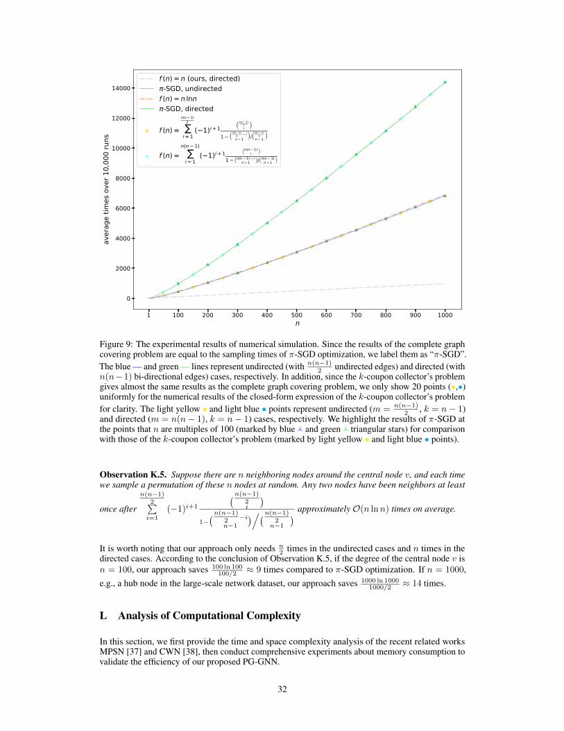
1 100 200 300 400 500 600 700 800 900 1000n

0

2000

4000

6000

8000

10000

12000

14000

aver

age

times

ove

r 10,

000

runs

f (n) = n (ours, directed)-SGD, undirected

f (n) = n lnn-SGD, directed

f (n) =n(n 1)

2

i = 1( 1)i + 1 (n(n 1)

2i )

1 (n(n 1)2 in 1 )/(n(n 1)

2n 1 )

f (n) =n(n 1)

i = 1( 1)i + 1 (n(n 1)

i )1 (n(n 1) i

n 1 )/(n(n 1)n 1 )

Figure 9: The experimental results of numerical simulation. Since the results of the complete graphcovering problem are equal to the sampling times of π-SGD optimization, we label them as “π-SGD”.The blue — and green — lines represent undirected (with n(n−1)

2 undirected edges) and directed (withn(n−1) bi-directional edges) cases, respectively. In addition, since the k-coupon collector’s problemgives almost the same results as the complete graph covering problem, we only show 20 points (•,•)uniformly for the numerical results of the closed-form expression of the k-coupon collector’s problemfor clarity. The light yellow • and light blue • points represent undirected (m = n(n−1)

2 , k = n− 1)and directed (m = n(n− 1), k = n− 1) cases, respectively. We highlight the results of π-SGD atthe points that n are multiples of 100 (marked by blue ) and green ) triangular stars) for comparisonwith those of the k-coupon collector’s problem (marked by light yellow • and light blue • points).

Observation K.5. Suppose there are n neighboring nodes around the central node v, and each timewe sample a permutation of these n nodes at random. Any two nodes have been neighbors at least

once after

n(n−1)2∑i=1

(−1)i+1

(n(n−1)2i

)1−(n(n−1)

2 −in−1

)/(n(n−1)2

n−1

) approximately O(n lnn) times on average.

It is worth noting that our approach only needs n2 times in the undirected cases and n times in the

directed cases. According to the conclusion of Observation K.5, if the degree of the central node v isn = 100, our approach saves 100 ln 100

100/2 ≈ 9 times compared to π-SGD optimization. If n = 1000,e.g., a hub node in the large-scale network dataset, our approach saves 1000 ln 1000

1000/2 ≈ 14 times.

L Analysis of Computational Complexity

In this section, we first provide the time and space complexity analysis of the recent related worksMPSN [37] and CWN [38], then conduct comprehensive experiments about memory consumption tovalidate the efficiency of our proposed PG-GNN.

32

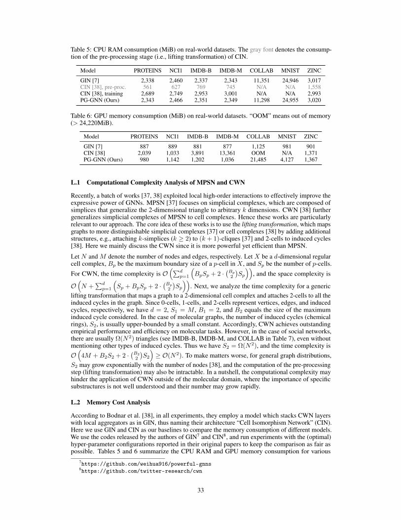
Table 5: CPU RAM consumption (MiB) on real-world datasets. The gray font denotes the consump-tion of the pre-processing stage (i.e., lifting transformation) of CIN.

Model PROTEINS NCI1 IMDB-B IMDB-M COLLAB MNIST ZINC

GIN [7] 2,338 2,460 2,337 2,343 11,351 24,946 3,017CIN [38], pre-proc. 561 627 769 745 N/A N/A 1,558CIN [38], training 2,689 2,749 2,953 3,001 N/A N/A 2,993PG-GNN (Ours) 2,343 2,466 2,351 2,349 11,298 24,955 3,020

Table 6: GPU memory consumption (MiB) on real-world datasets. “OOM” means out of memory(> 24,220MiB).

Model PROTEINS NCI1 IMDB-B IMDB-M COLLAB MNIST ZINC

GIN [7] 887 889 881 877 1,125 981 901CIN [38] 2,039 1,033 3,891 13,361 OOM N/A 1,371PG-GNN (Ours) 980 1,142 1,202 1,036 21,485 4,127 1,367

L.1 Computational Complexity Analysis of MPSN and CWN

Recently, a batch of works [37, 38] exploited local high-order interactions to effectively improve theexpressive power of GNNs. MPSN [37] focuses on simplicial complexes, which are composed ofsimplices that generalize the 2-dimensional triangle to arbitrary k dimensions. CWN [38] furthergeneralizes simplicial complexes of MPSN to cell complexes. Hence these works are particularlyrelevant to our approach. The core idea of these works is to use the lifting transformation, which mapsgraphs to more distinguishable simplicial complexes [37] or cell complexes [38] by adding additionalstructures, e.g., attaching k-simplices (k ≥ 2) to (k + 1)-cliques [37] and 2-cells to induced cycles[38]. Here we mainly discuss the CWN since it is more powerful yet efficient than MPSN.

Let N and M denote the number of nodes and edges, respectively. Let X be a d-dimensional regularcell complex, Bp be the maximum boundary size of a p-cell in X , and Sp be the number of p-cells.

For CWN, the time complexity is O(∑d

p=1

(BpSp + 2 ·

(Bp

2

)Sp

)), and the space complexity is

O(N +

∑dp=1

(Sp +BpSp + 2 ·

(Bp

2

)Sp

)). Next, we analyze the time complexity for a generic

lifting transformation that maps a graph to a 2-dimensional cell complex and attaches 2-cells to all theinduced cycles in the graph. Since 0-cells, 1-cells, and 2-cells represent vertices, edges, and inducedcycles, respectively, we have d = 2, S1 = M , B1 = 2, and B2 equals the size of the maximuminduced cycle considered. In the case of molecular graphs, the number of induced cycles (chemicalrings), S2, is usually upper-bounded by a small constant. Accordingly, CWN achieves outstandingempirical performance and efficiency on molecular tasks. However, in the case of social networks,there are usually Ω(N2) triangles (see IMDB-B, IMDB-M, and COLLAB in Table 7), even withoutmentioning other types of induced cycles. Thus we have S2 = Ω(N2), and the time complexity isO(

4M +B2S2 + 2 ·(B2

2

)S2

)≥ O(N2). To make matters worse, for general graph distributions,

S2 may grow exponentially with the number of nodes [38], and the computation of the pre-processingstep (lifting transformation) may also be intractable. In a nutshell, the computational complexity mayhinder the application of CWN outside of the molecular domain, where the importance of specificsubstructures is not well understood and their number may grow rapidly.

L.2 Memory Cost Analysis

According to Bodnar et al. [38], in all experiments, they employ a model which stacks CWN layerswith local aggregators as in GIN, thus naming their architecture “Cell Isomorphism Network” (CIN).Here we use GIN and CIN as our baselines to compare the memory consumption of different models.We use the codes released by the authors of GIN7 and CIN8, and run experiments with the (optimal)hyper-parameter configurations reported in their original papers to keep the comparison as fair aspossible. Tables 5 and 6 summarize the CPU RAM and GPU memory consumption for various

7https://github.com/weihua916/powerful-gnns8https://github.com/twitter-research/cwn

33

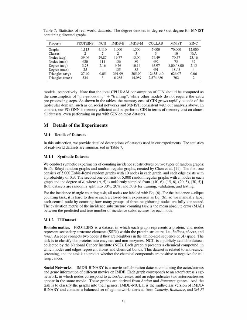
Table 7: Statistics of real-world datasets. The degree denotes in-degree / out-degree for MNISTcontaining directed graphs.

Property PROTEINS NCI1 IMDB-B IMDB-M COLLAB MNIST ZINC

Graphs 1,113 4,110 1,000 1,500 5,000 70,000 12,000Classes 2 2 2 3 3 10 N/ANodes (avg) 39.06 29.87 19.77 13.00 74.49 70.57 23.16Nodes (max) 620 111 136 89 492 75 37Degree (avg) 3.73 2.16 9.76 10.14 65.97 8.00 / 8.00 2.15Degree (max) 25 4 135 88 491 18 / 8 4Triangles (avg) 27.40 0.05 391.99 305.90 124551.40 626.07 0.06Triangles (max) 534 3 6,985 14,089 2,574,680 702 2

models, respectively. Note that the total CPU RAM consumption of CIN should be computed asthe consumption of “pre-processing” + “training”, while other models do not require the extrapre-processing steps. As shown in the tables, the memory cost of CIN grows rapidly outside of themolecular domain, such as on social networks and MNIST, consistent with our analysis above. Incontrast, our PG-GNN is memory-efficient and outperforms CIN in terms of memory cost on almostall datasets, even performing on par with GIN on most datasets.

M Details of the Experiments

M.1 Details of Datasets

In this subsection, we provide detailed descriptions of datasets used in our experiments. The statisticsof real-world datasets are summarized in Table 7.

M.1.1 Synthetic Datasets

We conduct synthetic experiments of counting incidence substructures on two types of random graphs:Erdos-Rényi random graphs and random regular graphs, created by Chen et al. [11]. The first oneconsists of 5,000 Erdos-Rényi random graphs with 10 nodes in each graph, and each edge exists witha probability of 0.3. The second one consists of 5,000 random regular graphs with n nodes in eachgraph and the degree of d, where (n, d) is uniformly sampled from (10, 6), (15, 6), (20, 5), (30, 5).Both datasets are randomly split into 30%, 20%, and 50% for training, validation, and testing.

For the incidence triangle counting task, all nodes are labeled with Eq. (6). For the incidence 4-cliquecounting task, it is hard to derive such a closed-form expression as Eq. (6), so we manually labeleach central node by counting how many groups of three neighboring nodes are fully connected.The evaluation metric of the incidence substructure counting task is the mean absolute error (MAE)between the predicted and true number of incidence substructures for each node.

M.1.2 TUDataset

Bioinformatics. PROTEINS is a dataset in which each graph represents a protein, and nodesrepresent secondary structure elements (SSEs) within the protein structure, i.e., helices, sheets, andturns. An edge connects two nodes if they are neighbors in the amino-acid sequence or 3D space. Thetask is to classify the proteins into enzymes and non-enzymes. NCI1 is a publicly available datasetcollected by the National Cancer Institute (NCI). Each graph represents a chemical compound, inwhich nodes and edges represent atoms and chemical bonds. This dataset is related to anti-cancerscreening, and the task is to predict whether the chemical compounds are positive or negative for celllung cancer.

Social Networks. IMDB-BINARY is a movie-collaboration dataset containing the actor/actressand genre information of different movies on IMDB. Each graph corresponds to an actor/actress’s egonetwork, in which nodes correspond to actors/actresses, and an edge indicates two actors/actressesappear in the same movie. These graphs are derived from Action and Romance genres. And thetask is to classify the graphs into their genres. IMDB-MULTI is the multi-class version of IMDB-BINARY and contains a balanced set of ego networks derived from Comedy, Romance, and Sci-Fi

34

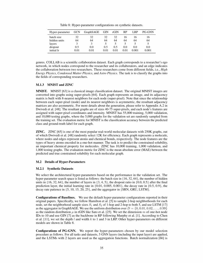
Table 8: Hyper-parameter configurations on synthetic datasets.

Hyper-parameter GCN GraphSAGE GIN rGIN RP LRP PG-GNN

batch size 32 32 32 32 16 16 16hidden units 64 64 64 64 64 64 64layers 3 3 5 5 5 5 5dropout 0.5 0.0 0.5 0.5 0.0 0.0 0.0initial lr 0.01 0.01 0.01 0.01 0.01 0.001 0.001

genres. COLLAB is a scientific collaboration dataset. Each graph corresponds to a researcher’s egonetwork, in which nodes correspond to the researcher and its collaborators, and an edge indicatesthe collaboration between two researchers. These researchers come from different fields, i.e., HighEnergy Physics, Condensed Matter Physics, and Astro Physics. The task is to classify the graphs intothe fields of corresponding researchers.

M.1.3 MNIST and ZINC

MNIST. MNIST [63] is a classical image classification dataset. The original MNIST images areconverted into graphs using super-pixels [64]. Each graph represents an image, and its adjacencymatrix is built with 8-nearest neighbors for each node (super-pixel). Note that since the relationshipbetween each super-pixel (node) and its nearest neighbors is asymmetric, the resultant adjacencymatrices are also asymmetric. For more details about the generation, please refer to Appendix A.2 inDwivedi et al. [48]. The resultant graphs are of sizes 40-75 super-pixels, and each node’s features areassigned with super-pixel coordinates and intensity. MNIST has 55,000 training, 5,000 validation,and 10,000 testing graphs, where the 5,000 graphs for the validation set are randomly sampled fromthe training set. The evaluation metric for MNIST is the classification accuracy between the predictedclass and ground-truth label for each graph.

ZINC. ZINC [65] is one of the most popular real-world molecular datasets with 250K graphs, outof which Dwivedi et al. [48] randomly select 12K for efficiency. Each graph represents a molecule,where nodes and edges represent atoms and chemical bonds, respectively. The node features are thetypes of heavy atoms encoded in a one-hot manner. The task is to predict the constrained solubility,an important chemical property for molecules. ZINC has 10,000 training, 1,000 validation, and1,000 testing graphs. The evaluation metric for ZINC is the mean absolute error (MAE) between thepredicted and true constrained solubility for each molecular graph.

M.2 Details of Hyper-Parameters

M.2.1 Synthetic Datasets

We select the architectural hyper-parameters based on the performance in the validation set. Thehyper-parameter search space is listed as follows: the batch size in 16, 32, 64, the number of hiddenunits in 16, 32, 64, the number of layers in 3, 4, 5, the dropout ratio in 0.0, 0.5 after the finalprediction layer, the initial learning rate in 0.01, 0.005, 0.001, the decay rate in 0.5, 0.9, thedecay rate patience in 5, 10, 15, 20, 25, and the aggregator in SRN, GRU, LSTM.

Configurations of Baselines. We use the default hyper-parameter configurations reported in theiroriginal papers. Specifically, we follow Hamilton et al. [5] to sample 2-hop neighborhoods for eachnode, set the neighborhood sample sizes S1 and S2 of 1-hop and 2-hop to both 5, and use LSTM [17]as the aggregator in GraphSAGE. We use the uniform distribution overD = 0, 0.01, 0.02, . . . , 0.99as the random distribution µ in rGIN like Sato et al. [25]. We set the dimension m of one-hot nodeIDs to 10 and use GIN [7] as the backbone in RP following Murphy et al. [1]. According to Chenet al. [11], we set the depth l and width k to 1 and 3 in LRP. Other hyper-parameters on differentmodels are shown in Table 8.

Configurations of PG-GNN. We report the hyper-parameters chosen by our model selectionprocedure as follows. For all tasks and datasets, 5 GNN layers (including the input layer) are applied,and the LSTMs with 2 layers are used as the aggregation functions. Batch normalization [66] is

35

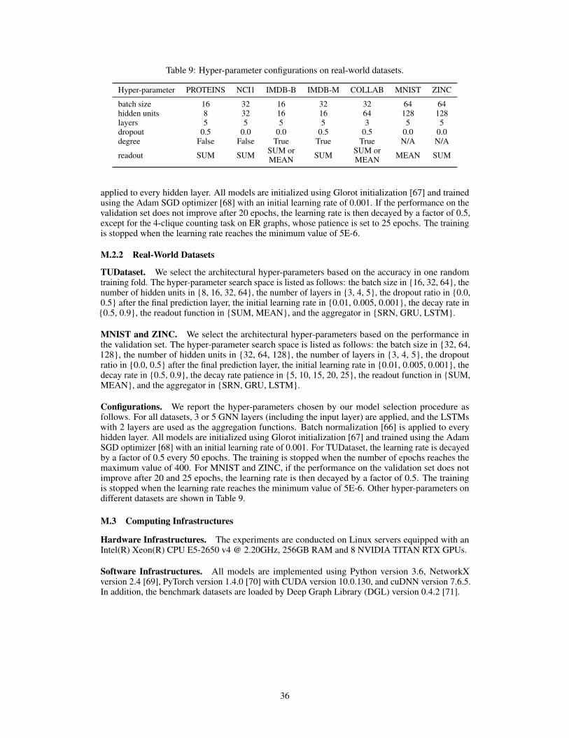
Table 9: Hyper-parameter configurations on real-world datasets.

Hyper-parameter PROTEINS NCI1 IMDB-B IMDB-M COLLAB MNIST ZINC

batch size 16 32 16 32 32 64 64hidden units 8 32 16 16 64 128 128layers 5 5 5 5 3 5 5dropout 0.5 0.0 0.0 0.5 0.5 0.0 0.0degree False False True True True N/A N/A

readout SUM SUM SUM orMEAN SUM SUM or

MEAN MEAN SUM

applied to every hidden layer. All models are initialized using Glorot initialization [67] and trainedusing the Adam SGD optimizer [68] with an initial learning rate of 0.001. If the performance on thevalidation set does not improve after 20 epochs, the learning rate is then decayed by a factor of 0.5,except for the 4-clique counting task on ER graphs, whose patience is set to 25 epochs. The trainingis stopped when the learning rate reaches the minimum value of 5E-6.

M.2.2 Real-World Datasets

TUDataset. We select the architectural hyper-parameters based on the accuracy in one randomtraining fold. The hyper-parameter search space is listed as follows: the batch size in 16, 32, 64, thenumber of hidden units in 8, 16, 32, 64, the number of layers in 3, 4, 5, the dropout ratio in 0.0,0.5 after the final prediction layer, the initial learning rate in 0.01, 0.005, 0.001, the decay rate in0.5, 0.9, the readout function in SUM, MEAN, and the aggregator in SRN, GRU, LSTM.

MNIST and ZINC. We select the architectural hyper-parameters based on the performance inthe validation set. The hyper-parameter search space is listed as follows: the batch size in 32, 64,128, the number of hidden units in 32, 64, 128, the number of layers in 3, 4, 5, the dropoutratio in 0.0, 0.5 after the final prediction layer, the initial learning rate in 0.01, 0.005, 0.001, thedecay rate in 0.5, 0.9, the decay rate patience in 5, 10, 15, 20, 25, the readout function in SUM,MEAN, and the aggregator in SRN, GRU, LSTM.

Configurations. We report the hyper-parameters chosen by our model selection procedure asfollows. For all datasets, 3 or 5 GNN layers (including the input layer) are applied, and the LSTMswith 2 layers are used as the aggregation functions. Batch normalization [66] is applied to everyhidden layer. All models are initialized using Glorot initialization [67] and trained using the AdamSGD optimizer [68] with an initial learning rate of 0.001. For TUDataset, the learning rate is decayedby a factor of 0.5 every 50 epochs. The training is stopped when the number of epochs reaches themaximum value of 400. For MNIST and ZINC, if the performance on the validation set does notimprove after 20 and 25 epochs, the learning rate is then decayed by a factor of 0.5. The trainingis stopped when the learning rate reaches the minimum value of 5E-6. Other hyper-parameters ondifferent datasets are shown in Table 9.

M.3 Computing Infrastructures

Hardware Infrastructures. The experiments are conducted on Linux servers equipped with anIntel(R) Xeon(R) CPU E5-2650 v4 @ 2.20GHz, 256GB RAM and 8 NVIDIA TITAN RTX GPUs.

Software Infrastructures. All models are implemented using Python version 3.6, NetworkXversion 2.4 [69], PyTorch version 1.4.0 [70] with CUDA version 10.0.130, and cuDNN version 7.6.5.In addition, the benchmark datasets are loaded by Deep Graph Library (DGL) version 0.4.2 [71].

36