Global Warming Effect Applied to Electricity Generation Technologies by Sergio Almeida Pacca Agronomy (University of Sao Paulo, Brazil) 1987 Social Sciences (University of Sao Paulo, Brazil) 1992 M.S. (University of Sao Paulo, Brazil) 1997 A dissertation submitted in partial satisfaction of the requirements for the degree of Doctor of Philosophy in Energy and Resources in the GRADUATE DIVISION of the UNIVERSITY OF CALIFORNIA, BERKELEY Committee in charge: Professor Arpad Horvath (Chair) Professor Richard Norgaard Professor Daniel Kammen Professor Dennis Baldocchi Spring 2003

Welcome message from author
This document is posted to help you gain knowledge. Please leave a comment to let me know what you think about it! Share it to your friends and learn new things together.
Transcript
Global Warming Effect Applied to Electricity Generation Technologies
by
Sergio Almeida Pacca
Agronomy (University of Sao Paulo, Brazil) 1987
Social Sciences (University of Sao Paulo, Brazil) 1992
M.S. (University of Sao Paulo, Brazil) 1997
A dissertation submitted in partial satisfaction of the requirements for the degree of
Doctor of Philosophy
in
Energy and Resources
in the
GRADUATE DIVISION
of the
UNIVERSITY OF CALIFORNIA, BERKELEY
Committee in charge:
Professor Arpad Horvath (Chair)
Professor Richard Norgaard
Professor Daniel Kammen
Professor Dennis Baldocchi
Spring 2003

The dissertation of Sergio Almeida Pacca is approved:
Chair Date
Date
Date
Date
University of California, Berkeley
Spring 2003
Global Warming Effect:
A Climate Change Mitigation Option Targeting Electricity Generation Technologies
Copyright (©2003)
by
Sergio Almeida Pacca
3/27/2003
Abstract
Global Warming Effect:
A Climate Change Mitigation Option Targeting Electricity Generation Technologies
by
Sergio Almeida Pacca
Doctor of Philosophy in Enegy and Resources
University of California, Berkeley
Professor Arpad Horvath, Chair
ABSTRACT GOES HERE
3/27/2003
i
TABLE OF CONTENTS:
List of Figures ......................................................................................................................................iii
List of Tables .......................................................................................................................................iv
List of Acronyms.................................................................................................................................vi
List of Symbols ..................................................................................................................................viii
Acknowledgments...............................................................................................................................ix
Chapter 1: Introduction .................................................................................................................1
Chapter 2: Life-cycle Assessment (LCA) Precursors to Compare Electricity Generation
Options .................................................................................................................5
2.1 LCA in Energy Analysis ........................................................................................................6
2.2 Comparison of Energy Technologies and Climate Change ...........................................11
2.2.1 Benefit-Cost Analysis (BCA) Applied to Climate Change.......................................13
2.2.1.1 Economic Discounting ..........................................................................................13
2.2.1.2 Economic Valuation...............................................................................................18
Chapter 3: Assessment Method and Approach ............................................................................22
3.1 The Global Warming Effect (GWE) Method..................................................................22
3.2 Problems and Uncertainties Associated with the Assessment Method........................26
3.2.1 Problems with LCA.......................................................................................................27
3.2.2 Problems with the Global Warming Potential (GWP) ............................................36
3.2.2.1 Problems with Radiative Efficiency .....................................................................39
3.2.2.2 Problems with the Modeling of Stocks and Flows of Greenhouse Gases
(GHGs) ...............................................................................................................45
3.2.2.3 Carbon Cycle Models and Pulse Response Functions (PRFs) .........................47
3.2.2.4 Parameters Used in the Calculation of GWPs and GWEs...............................58
Chapter 4: Electricity Generation Case Studies ............................................................................61
4.1 Hydroelectric Plants .............................................................................................................62
4.1.1 Carbon Balance Between Air and Reservoirs ............................................................64
4.1.1.1 Potential Emissions from Decomposition of Flooded Carbon.......................65
4.1.1.2 Net Ecosystem Production Balance.....................................................................67
4.1.2 Hydroelectricity Case Studies.......................................................................................70
4.1.2.1 Glen Canyon Dam..................................................................................................73
3/27/2003
ii
4.1.2.2 Tucurui Hydroelectric Plant ..................................................................................77
4.2 Photovoltaic Electricity Generation Systems ...................................................................83
4.2.1 Global Warming Effect of a PV System ....................................................................96
4.2.1.1 PV System in a Dry Ecosystem ............................................................................96
4.2.1.2 PV System in a Tropical Forest ......................................................................... 100
4.3 Wind .................................................................................................................................... 103
4.3.1 Global Warming Effect of a Wind Farm in the U.S.............................................. 106
4.4 Coal...................................................................................................................................... 108
4.4.1 Global Warming Effect of a Coal Fired Power Plant ........................................... 116
4.5 Natural Gas......................................................................................................................... 119
4.5.1 Natural Gas Power Plant in the U.S. ....................................................................... 122
4.5.2 Natural Gas Power Plant in Brazil ........................................................................... 124
4.6 Problems from Dimensioning and Characterization of Power Plants ...................... 126
Chapter 5: Discussion and Interpretation of Results................................................................ 128
Chapter 6: Use of GWE in Environmental Policy and Management .................................... 134
Chapter 7: Dissertation Contribution.......................................................................................... 138
Chapter 8: Future Work and Research Needs ........................................................................... 143
Literature Cited................................................................................................................................ 146

3/27/2003
iii
LIST OF FIGURES
Figure 1 : Phases of a Product or Service in a LCA......................................................................11
Figure 2 : Changes in Value and Atmospheric Concentration of Carbon Dioxide..................16
Figure 3 : Problems with LCA .........................................................................................................28
Figure 4 : Energy Efficiency Index for Iron and Steel Production [Metz 2001]. .....................33
Figure 5 : Global Climatic Features not Explicitly Treated in the GWP Method....................37
Figure 6 : Global and Annual Mean Radiative Forcing (1750 to present) [Houghton 2001]. 41
Figure 7 : HILDA Model [Siegenthaler 1992] ..............................................................................50
Figure 8 : Independend Variables Affecting Projected Carbon Background Concentrations53
Figure 9 : Future Carbon Emissions and Carbon Dioxide Concentrations ..............................56
Figure 10 : PRFs Based on TAR Scenarios and PR Model Used in the Calculation of GWP.
..............................................................................................................................................57
Figure 11 : Present Day Emissions and Sinks of Carbon [Einsele 2001] ..................................69
Figure 12 : Electricity Generation Alternatives and Impact Categories Considered in This
Assessment..........................................................................................................................72
Figure 13 : Learning Curve for PV Modules [IEA 2000b] ..........................................................89
Figure 14 : Materials and Energy inputs in Different Grid Connected Systems (kg/kWp)
[Dones 1998] ......................................................................................................................92
Figure 15 : Electricity Costs and CO2 Emissions Versus System Lifetime [Oliver 2000] .......95
Figure 16 : Coal Power Generation Life-cycle Phases............................................................... 108
Figure 17 : Carbon Dioxide Emissions by Coal Ranking and Geographical Location......... 111
Figure 18 : Average Distance of Coal Shipments by Rail in the U.S., 1988-1997 [U.S. EIA
2000] ................................................................................................................................. 113
Figure 19 : Comparison of GWE for GCD with Four Other Alternatives and Four Time
Periods After Construction (g of CO2 equiv./kWh). ................................................ 128
Figure 20 : Estimation and Sensitivity Analysis of GWE for Electricity Generation Options
Over Four Different Periods of Analysis.................................................................... 129
Figure 21 : Carbon Dioxide Emissions from Combustion and Foregone Carbon Dioxide
Uptake due to NEP. ....................................................................................................... 131
Figure 22 : Sensitivity Analysis of the Tucurui Hydroelectric Power Plant Design Assuming
Different Ecosystem Types........................................................................................... 132

3/27/2003
iv
LIST OF TABLES
Table 1 : Simplified Expression for Calculation of CO2 ∆F in W/m2 [Houghton 2001]........43
Table 2 : Simplified Expression for GHGs ∆F calculations in W/m2 [Houghton 2001] .......44
Table 3 : Scenarios Storylines ...........................................................................................................55
Table 4 : Releases of CO2 and CH4 from Reservoirs. ...................................................................66
Table 5 : Glen Canyon Hydroelectric Plant Construction Inputs and GWE (after 20 yr of
operation) [Pacca 2002].....................................................................................................75
Table 6 : Characteristics of the Turbine Generator Sets in Tucurui [La Rovere 2000] ...........79
Table 7 : Major Construction Inputs and GWE (after 20 yr of operation) for Tucurui
Hydroelectric Planta ...........................................................................................................82
Table 8 : Published Carbon Dioxide Emissions per Kilowatt-hour for PV Systems. .............84
Table 9 : Characteristic Parameters in a PV installation. ..............................................................86
Table 10 : Energy Requirements for Module Manufacturing (MJ/m2) (Adapted from
[Alsema 2000])....................................................................................................................87
Table 11 : Energy Inputs into System Components: [Alsema 2000b] .......................................91
Table 12 : Major Construction Inputs and GWE (after 20 yr) for a PV Plant .........................99
Table 13 : Major Construction Inputs and GWE (after 20 yr of operation) for a PV Plant in
Brazila ................................................................................................................................ 102
Table 14 : Published Carbon Dioxide Emissions per Kilowatt-hour for Wind Farms ........ 104
Table 15 : Material Inputs in Wind Farms as a Percentage of the Total Mass....................... 105
Table 16 : Major Construction Inputs and GWE (after 20 yr of operation) for a Wind Farm
in the U.S.......................................................................................................................... 107
Table 17 : Published Carbon Dioxide Emissions per Kilowatt-hour for Coal-fired Power
Plants. ............................................................................................................................... 109
Table 18 : Life-cycle Material Inputs by Technology and Information Source (kg/GWh) . 115
Table 19 : Major Construction Inputs and GWE (after 20 yr of operation) for a Coal Power
Plant .................................................................................................................................. 118
Table 20 : Performance of Natural Gas Generation Technologies [CEC 1997] ................... 119
Table 21 : Published Carbon Dioxide Emissions per Kilowatt-hour for Natural Gas fueled
Plants. ............................................................................................................................... 121

3/27/2003
v
Table 22 : Major Construction Inputs and GWE (after 20 yr) for a Natural Gas Power Plant
........................................................................................................................................... 123
Table 23 : Major Construction Inputs and GWE (after 20 yr) for a Natural Gas Power Plant
........................................................................................................................................... 125
3/27/2003
vi
LIST OF ACRONYMS
AFBC atmospheric fluidized bed combustion plant
BOS balance of the system
BC black carbon
BCA benefit cost analysis
BEA Bureau of Economic Analysis
Btu British thermal unit
CPI consumer price index
EEI energy efficiency index
EIO-LCA economic input-output life-cycle assessment
ELN Eletronorte
GHG greenhouse gas
GWE global warming effect
GWh gigawatt-hour
GWP global warming potential
HILDA high latitude exchange/interior diffusion advection
IGCC integrated gasification combined cycle
IPCC intergovernmental panel on climate change
kWp kilowatt peak – photovoltaic module capacity
LCA life-cycle assessment
LEBS low emission boiler systems
m-Si mono-crystalline silicon
MCFC molten carbonate fuel cells
MTC metric tons of carbon
MTCO2Eq metric tons of carbon dioxide equivalent
MW megawatt
NEA net energy analysis
NREL National Renewable Energy Laboratory
NSPS new source performance standards
NTEL National Energy Technology Laboratory
Pg petagrams

3/27/2003
vii
p-Si poly-crystalline silicon
ppb parts per billion
ppm parts per million
SETAC Society of Environmental Toxicology and Chemistry
TAR third assessment report from the IPCC
EIA U.S. Energy Information Administration
EPA U.S. Environmental Protection Agency
OMB U.S. Office of Management and Budget
USBR U.S. Bureau of Reclamation

3/27/2003
viii
LIST OF SYMBOLS
C carbon
CH4 methane
CO2 carbon dioxide
N2O nitrous oxide
NOx nitrogen oxides
CuO copper oxide
SO2 sulfur dioxide

3/27/2003
ix
ACKNOWLEDGMENTS
The completion of my dissertation is a moment to reflect on my experiences throughout my
tenure at UC Berkeley and thank the scholars that shaped my life. I have had the opportunity
to learn with very distinguished professors. First, I would like to thank Professor Arpad
Horvath for his friendship, his very special guidance both with my preparation and with the
production of this dissertation. His course CE 268E Civil Systems and the Environment was
seminal to my dissertation research. The opportunity to collaborate with Professor Horvath
on various research projects allowed me to learn from a very fine scholar with an impressive
organizational capacity.
I am tremendously grateful to Professor Richard Norgaard, who is responsible for molding
my current research. Professor Norgaard has always available to critically discuss my
research ideas, contributed with various insights, and pointed me to various sources of
information. His courses ER 290 Energy Economics and ER 190 Ecological Economics have
changed my perception about environmental issues.
Next, I want to thank two scholars who are amongst the smartest scholars that I have met
on campus. Professor Daniel Kammen and Professor Dennis Baldocchi are truly the
representatives of the future of science at Berkeley and beyond. They are resourceful,
productive, and objective researchers, who have definitely motivated my own work.
I would not get to this point without the collaboration with Professor Catherine Koshland
and Professor Gene Rochlin who participated in my qualifying exam, and also contributed
with creative ideas and invaluable references. It was an exceptional opportunity to work as a

3/27/2003
x
teaching assistant for Professors Koshland and Kammen in their ER 100 Energy and Society
course.
Additionally, I want to thank my sponsors: The Conselho Nacional de Pesquisa (Brazil) that
supported my first four years as a graduate student, and the UC Toxics Research and
Training Program, which supported me afterwards.
Finally, I would like to thank the people of the Energy and Resources Group (ERG), and the
Consortium of Green Design and Manufacturing (CGDM), and my colleagues, the
incredible smart and motivated students, who contributed to a smooth journey to graduation.
3/27/2003
1
Chapter 1: Introduction
Climate change is a global problem in a complex realm of interactions between climatic,
environmental, economic, political, institutional, social and technological processes. Effects
of climate change manifest over long time horizons and any action taken now will affect our
sustainable development. Anthropogenic releases of greenhouse gases (GHGs) in the
biosphere are the major cause for climate change, and electricity generation accounts for 2.1
Gt yr-1 (Giga metric tons of carbon per year) or 37.5% of total global carbon emissions
[Metz 2001]. Lower GHGs emission scenarios require different patterns of energy
development and there is no single path to a low emission future. This work proposes a
framework to support the selection of the electricity generation technology with the lowest
global warming effect (GWE) amongst a set of available, feasible alternatives. The intent is
to reconcile local decisions with a global development path to minimize climate change.
The design of the research framework and the creation of a spreadsheet-based decision-
support tool, intend to be transparent and flexible. The user is encouraged to change
parameters and input the data that she understands is the most relevant for each analysis. By
applying the framework, the users should not only be concerned with the final results but
with the process itself. To facilitate that discernment, this work presents a systematization of
the sources of problems and uncertainties embedded in each of the components of the
framework.
Consequently, potential users of the GWE are analysts who recognize that the selection of
electricity generation technologies to mitigate climate change involves a set of assumptions,
choices, and uncertainties that affect the result of the assessment. Dealing with this set of
3/27/2003
2
variables is fundamental in any environmental policy analysis, and therefore, students who
are getting engaged in quantitative policy analysis could benefit from the GWE framework.
Decision-makers interested in the mitigation of climate change may benefit from the GWE
framework to initiate programs supporting technologies that reduce the burden of climate
change over time frames tailored to their needs. Analysts working for agencies, development
banks and foundations that solicit energy projects may benefit from the GWE to assess the
performance of different proposed alternatives. The industry involved in the manufacturing
of power plant components and electricity generation technologies may use the GWE
framework to identify ways of improving the performance of their products and services. In
summary, the GWE framework is designed to support the work of a range of users who are
committed to the mitigation of climate change.
The present dissertation is organized into eight chapters. In Chapter 2, a brief literature
review is presented followed by a discussion of the methods that are characterized as
precursors of the life-cycle assessment (LCA) method, which is a component of the GWE.
Methods focusing on energy use that were motivated by the oil crisis in the 1970s and lately
evolved into energy payback calculations are reviewed. Methods that attempt to identify
carbon dioxide (CO2) emissions over the full fuel cycle of a power plant are also amongst the
LCA precursors that have been applied to energy analysis.
Next, a more up to date alternative already focusing on climate change impacts and using
current LCA methods is discussed. LCA is one of the pillars of the GWE method, which
aggregates the fundamental systemic view of LCA into the time-integrated analysis derived
from climate change science. The temporal dimension characteristic of the climate change
science is incorporated into the GWE method as an alternative to time-dependent economic

3/27/2003
3
analysis. Indeed, if the concern is the comparison of power sources over time based on their
global impacts, alternatively economic tools such as benefit-cost analysis (BCA) could be
used. The chapter ends with a discussion of BCA applied to climate change and the
problems associated with the use of this technique. A critique of BCA calls for the use of
competing methods that are also able to compare the performance of technologies based on
their environmental impacts over flexible analytical periods.
In chapter 3, the GWE framework is explained. It is proposed in this dissertation in order to
compare electricity generation options based on their relative impact on global climate
change is explained. The GWE intends to be transparent enough to reveal choices,
assumptions, and uncertainties involved in the analysis. The method is composed of two
well-established methods: LCA and Global Warming Potential (GWP). Because the
framework aggregates different methods and these methods rely on other methods and
models, there is a chain of problems that are discussed with clarity to validate the framework.
A classification composed of three sources of problems is proposed:
1. problems related to the LCA method
2. problems related to the GWP method
3. problems related to the characterization of power plants
For each class a sub-classification is presented to help the user of the framework with the
identification of choices and uncertainties involved with the adoption of the GWE
framework.

3/27/2003
4
In chapter 4, various electricity case studies involving the use of the framework are presented.
The selection of different case studies aims to explore the variability associated with different
electricity supply options. In terms of technologies, hydroelectric plants, solar photovoltaic
(PV) modules, wind turbines, coal fired power plants, and natural gas fueled plants, are
considered. Potentially, the application of the GWE can be extended to other electricity
supply technologies and to any other technology currently in operation or expected in the
future.
In chapter 5, the results from the case studies presented in chapter 4 are discussed and
compared with the range of values identified in the literature for each of the electricity
supply technologies.
In chapter 6, the adequacy of the GWE as a decision support tool is discussed emphasizing
the use of the framework in environmental policy and management.
In chapter 7, the contribution of this research is presented.
In chapter 8, future work and research needs are described.
3/27/2003
5
Chapter 2: Life-cycle Assessment (LCA) Precursors to Compare
Electricity Generation Options
Frameworks for analyzing the performance of electricity supply options by looking at the
complete life-cycle of processes have existed for some time. Most of these frameworks
evolved from concerns with the oil shortage in the late 1970s, and attempted to reduce fossil
fuel consumption over the life-cycle of power plants. The origin of such studies goes back to
net energy analysis (NEA), a term coined to assess the energy input-output ratio of energy
supply and conservation technologies. Usually these studies looked at more traditional
sources of energy such as coal, oil, gas, hydro, and nuclear [Chapman 1974, Chapman 1975]
but some also looked at renewable sources [Haack 1981, Herendeen 1981]. NEA aims to
measure all energy flows associated with energy technologies during their different phases
using either input-output techniques or process analysis. The adoption of such approach was
recommended in the Non Nuclear Energy Research and Development Act of 1974 in the
U.S. [Leach 1975].
Nevertheless, the definition of NEA was not precise enough to spur its application. Fuel
cycle studies, which appeared in the late 1980s, are based on the same logic as NEAs. In
addition to the concern with energy consumption, analysts became also concerned with the
incorporation of environmental impacts, and the extension from energy to carbon emissions
was natural since most energy sources rely on fossil fuels combustion that releases carbon
dioxide.
Total fuel cycle studies capture the whole chain of carbon dioxide emissions during materials
production, construction, operation and decommissioning of power plants [Meridian Corp.

3/27/2003
6
1989, San Martin 1989, Uchiyama 1991, Uchiyama 1992]. Results are reported in metric tons
of CO2 per energy output (GWh) [Meridian Corp. 1989, San Martin 1989] Those studies
were based on the identification of fuel consumption in each of the life phases of the project
and its conversion to an environmental indicator such as CO2 emissions. However, this
method was unable to capture secondary impacts pertaining to the energy chain coupled to
the generation of electricity [Meridian Corp. 1989].
The need for an analytical framework that broadens the operation of electricity production
systems became fundamental for analyzing and comparing different alternatives. In the case
of PV systems, the necessity to prove that they were net energy sources led to life-cycle
based energy payback calculations including all direct and indirect energy inputs in the
fabrication and installation of the systems. This assessment was broader, and included
indirect energy used in the production chain of the modules and other parts of the PV
systems. The energy payback time indicates the time necessary to match energy inputs in the
facility with its energy yields [Alsema 2000].
2.1 LCA in Energy Analysis
Presently, life-cycle assessment (LCA) is applied to address the consumption of energy and
materials over the life of power plants [Uchiyama 2002, Gagnon 2002]. The goal of a LCA is
to quantify material and energy resource inputs as well as waste and pollutants outputs in the
production of a product or service. The method attempts to systematically quantify the
Energy Payback Time = Life-cycle primary energy consumed by the generation sytem (kWh)
Annual power generation (kWh/yr) (1)
3/27/2003
7
environmental effects of the various stages of a product or process life-cycle: materials
extraction, manufacturing/production, use/operation, and ultimate disposal (or end-of-life).
The challenge is to map production processes so that they accurately represent current
industry practices and trends. Several LCA tools provide process descriptions and flow
diagrams, and libraries of data to users in order to help the execution of LCA [Gabi 3 2003,
SimaPro 5 2003]. Existing studies differ in the number of environmental effects quantified,
and in the scope of the analysis (where the boundary of the analysis is drawn). Currently,
there are two major approaches to boundary setting: a process-based model developed most
intensively by the Society for Environmental Toxicology and Chemistry (SETAC) and the
U.S. Environmental Protection Agency (EPA) [Curran 1996], and an economic input-output
analysis-based model called EIO-LCA [EIO-LCA 2003, Hendrickson 1998]. The SETAC
approach has a more flexible boundary, which usually is selected at the discretion of the
analyst and is molded based on a specific case study. The boundary of input-output based
LCAs is predisposed by the boundary of the economic system from which data are extracted.
One strength of the input-output analytical framework is its completeness regarding the
coverage of the inputs in a given product or sector [Lenzen 2001].
In comparison, the SETAC-EPA approach divides each product into individual process
flows, and strives to quantify their environmental effects. This LCA comprises four major
components. First, the goal and scope definition establishes the objective of the analysis and
what criteria best represent the performance of the assessed alternatives to accomplish the
chosen objective. Second, the inventory analysis attempts to identify the major material and
energy inputs associated with the production of the subject of the assessment. Third, during
the impact assessment the effects arising from the use of each input in the production of the

3/27/2003
8
good are quantified and finally aggregated to yield the life-cycle impact of the object of the
analysis. Fourth, results are interpreted by means of comparisons, rankings, sensitivity
analyses, simulations, etc.
The inventory analysis of the SETAC-EPA method is constrained by the perceptionof the
analyst on what is important to be quantified. For example, in the manufacturing stage of
products, the analyst attempts to trace inputs as far back (“upstream”) in the production
chain as possible. This assessment is typically limited by data availability, time and cost, and
includes the first tier (direct) suppliers, but seldom the complete hierarchy of suppliers, i.e.,
all the suppliers of suppliers (and thus the indirect effects). A problem defined as “truncation
error” reflects the omission of some of the processes in the production chain and in the final
results of the analysis from the boundary selection of this kind of LCA [Lenzen 2001].
In contrast, input-output based approaches essentially enclose all upstream production
phases. The EIO-LCA model uses the 498x498 economic input-output commodity-by-
commodity matrix of the U.S. economy (a general interdependency model) to identify the
entire chain of suppliers (both direct and indirect) of a commodity. In this case, the
boundary of the assessment is set at the national economy level. The 498x498 matrix is
based on commodities such as cement, steel, coal, sugar, etc. To obtain the total (direct plus
indirect) economic demand, final purchase (final demand) amounts are specified to the
model. The results are then multiplied by matrices of energy use and emission factors
calculated by economic sector level (e.g., energy use per dollar). The base year for EIO-LCA
data is currently 1997. The EIO-LCA model has been applied to a number of product
assessments [see, e.g., Lave 2000, Horvath 1998a, Horvath 1998b].
3/27/2003
9
The EIO-LCA method is comprehensive and covers all commodities exchanged in a given
economy. On the one hand, the selection of a national or regional economy establishes well
defined boundaries for the calculation of emission factors. On the other hand, such emission
factors are averages that correspond to a mix of agents (producers, service providers, etc)
developing the same activity within the given economy. Averages do not represent the
performance of a specific agent within an economic sector, who may be above or below the
average performance of the sector, nor it represents the performance of a foreign producer
that sells her products in the American market, which is modeled by the EIO-LCA. In order
to deal with this particular problem, EIO-LCA assumes that imported goods are produced
similarly to domestic goods.
Depending on the intent of the analyst the use of emission factors provided by EIO-LCA
may lead to inaccurate emission factors for a given product. This is due to the aggregation
level of the sectors modeled. Each specific sector modeled by the Bureau of Economic
Analysis (BEA) is in fact a bundle of goods and services that in some cases are very disparate,
and therefore, products or services within the same sector may actually lead to completely
different emission factors.
In addition to a classification problem that averages the emission factors for products and
services that involve different production chains and technologies, different emission factors
for the production of the same commodity are also possible because of the technological
heterogeneity amongst producers that manufacture a similar final product.
Knowledge about technology is also important because technology is dynamic and due to
the time involved with data collection and information treatment there is always a time lag
between the EIO-LCA data and the current technology. The magnitude of this problem
3/27/2003
10
varies according to the product and sector because some sectors are quite stable in terms of
technological innovation, whereas other sectors change their technology more rapidly.
Temporal changes also affect the use of emission factors from EIO-LCA because they are
based on prices and prices are relative and change over time. Finally, the issue of technology
spans over differences in scale between different firms. A given technology may be more
adequate for a small sized firm with a small output but when the scale is larger another
technology may be more appropriate.
The problems with the LCA part of the GWE framework are discussed in detail in section
3.2.1. In order to provide an organized view about problems arising from the use of LCA
the following classification is proposed: data, temporal constraint, economic boundary, and
methodological constraints. Data problems are associated with the collection and treatment
of the information, temporal problems address the effects of time in the results from LCAs,
economic boundary problems are related to the choice of economic transactions to
intermediate the flows of commodities, energy and pollution within a specific territory, and
methodological constraints are related with mathematical presumptions in the model such as
linear relationships.
Even if the application of the EIO-LCA needs to be supported by knowledge on its
limitations and the use of a process LCA has other sorts of problems, the structure of energy
generation systems demands a life-cycle approach to reveal the potential of an alternative to
achieve increased performance and reduce emissions [Nieuwlaar 1996]. Indeed, LCA is
fundamental to assess any kind of technology, especially in the case of climate change
because the location of the emission sources does not affect the potential impacts. That is,
the global warming effect is global in comparison to effects from regional pollutants.
3/27/2003
11
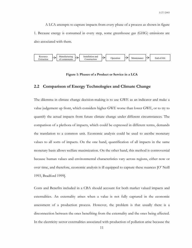
A LCA attempts to capture impacts from every phase of a process as shown in figure
1. Because energy is consumed in every step, some greenhouse gas (GHG) emissions are
also associated with them.
Figure 1: Phases of a Product or Service in a LCA
2.2 Comparison of Energy Technologies and Climate Change
The dilemma in climate change decision-making is to use GWE as an indicator and make a
value judgement up front, which considers higher GWE worse than lower GWE, or to try to
quantify the actual impacts from future climate change under different circumstances. The
comparison of a plethora of impacts, which could be expressed in different terms, demands
the translation to a common unit. Economic analysis could be used to ascribe monetary
values to all sorts of impacts. On the one hand, quantification of all impacts in the same
monetary basis allows welfare maximization. On the other hand, this method is controversial
because human values and environmental characteristics vary across regions, either now or
over time, and therefore, economic analysis is ill equipped to capture these nuances [O' Neill
1993, Bradford 1999].
Costs and Benefits included in a CBA should account for both market valued impacts and
externalities. An externality arises when a value is not fully captured in the economic
assessment of a production process. However, the problem is that usually there is a
disconnection between the ones benefiting from the externality and the ones being affected.
In the electricity sector externalities associated with production of pollution arise because the
Manufacturing of components
Installation and Construction Maintenance End-of-life Operation
Resource Extraction

3/27/2003
12
value of the damage caused by pollution elsewhere is not included amongst the costs of the
electricity producer. The solution to this problem is in part associated with the establishment
of property rights coupled to the elements affected by pollution. A subsidy for the electricity
generator is another example of externalities for this sector. In this case the cost of an input
used by the producer to generate electricity is below market prices. Tax and insurance
differentiation, distortion in markets for labor, land, and energy resources also contribute for
the production of externalities in the electricity sector. The existence of externalities distorts
the prices, and therefore, the results of an economic analysis depend on how externalities are
defined, identified, and evaluated. This is another drawback for the use of economics
because it challenges the claim that economic analysis produces a unique and precise answer
for any resource allocation problem. In the case of climate change the disconnection
between the ones benefiting from the use of energy and the ones affected by the emissions
of greenhouse gases and their impacts on the global climate is a temporal problem that can
be framed as a intergenerational equity issue.
In this work I attempt to compare the global environmental performance of different
electricity supply technologies over time using the GWE method. Alternatively, economic
analysis could be used in the comparison and probably the causalities of climate change,
which are discussed with some level of detail in this study, would be implicit in a Benefit
Cost Analysis (BCA)-like analysis. Besides, if a BCA framework is chosen, instead of
comparing the effect of GHGs over time I would be comparing economic values over time
and one problem that would arise is the selection of an appropriate discount rate to compare
alternatives over time. In short, similarly to what happens to GWE’s formulation

3/27/2003
13
assumptions and uncertainties are also associated with BCA. These problems are briefly
discussed in the next sections.
2.2.1 Benefit-Cost Analysis (BCA) Applied to Climate Change
BCA is the conventional economic approach to design public policy [Nordhaus 1999]. In
addition, some economists claim that sustainability issues are addressed through BCA
[Howarth 1995]. Accordingly, the use of economic analysis to evaluate outcomes from
future climate change has been widely discussed by the Working Group III of the
Intergovernmental Panel on Climate Change (IPCC) which was structured to assess “cross-
cutting economic and other issues related to climate change.” The IPCC second assessment
report is not conclusive but acknowledges the difficulty to assess benefits and costs related
to climate change effects in economic terms [Bruce 1996].
When economists deal with values in the future, which is the case with climate change, they
look at the stream of future values in terms of their net present value. Therefore, the trade-
off between consumption today and consumption in the future raises two central questions:
first, how to think about this trade-off; second, what numerical value to attach to it. [Bruce
1996]. The first problem lies on the discussion of economic discounting, the second one
relates to a pure valuation problem.
2.2.1.1 Economic Discounting
Economic discounting issues arise when economic outcomes associated with a stream of
benefits and costs over time are compared using discount rates that translate future values

3/27/2003
14
into present values. This comparison is particularly important if we ponder that for
economists sustainability is a matter of intergenerational equity or how resources are
distributed between generations [Howarth 1992].
Discount rates embody different factors, which change the value of money over time, such
as interest rates, inflation, and taxes. Interest rates are probably the most interesting
component because they are intertwined with a great variety of forces, chiefly independent
of the particular commodity and industry in question [Hotteling 1931]. Private interest rates
reflect the anxiety of consumers and the marginal productivity of invested capital, and both
of them depend on the equilibrium of the market economy.
In traditional BCA, the weight attributed to benefit and costs at different times is critical and
is determined by the discount rate used. The higher the discount rate the lower future
benefits and costs are when compared to present ones. The choice of market discount rates
to deal with environmental problems steaming from energy use has been challenged because
of some intricacies associated with the matter. The use of current market discount rates
would reveal a myopic view of the distribution of benefits and costs over time because long
time frames, which are not reflected in market discount rates, characterize natural processes
associated with energy technologies [Lind 1982].
For example, in the case of nuclear power the use of a 10 % discount rate, as was specified
by the U.S. Office of Management and Budget (OMB), converts high environmental costs
such as the disposal of nuclear waste, to a negligible present value [Lind 1982]. A similar
problem occurs with climate change because natural processes controlling the atmosphere,
the oceans and ecosystems are characterized by long time frames, for example:
3/27/2003
15
• decades to centuries are necessary to balance the climate system given a stable level of
GHG concentrations,
• centuries are necessary to equilibrate sea level given a stable climate,
• decades to centuries are necessary to restore/rehabilitate damaged or disturbed ecological
systems, and moreover, some changes are irreversible.
• decades to millennia are necessary to balance atmospheric concentrations of long-lived
green-house gases given a stable level of GHG emissions,
As a matter of fact, a natural process, such as carbon dioxide decay in the biosphere entails a
discount rate for capital, which is usually much less than is considered in economic
appraisals of federal projects. The Appendix C of the Circular No. A-94 published by the
Office of Management and Budget (OMB) of the White House stipulates real interest rates
on treasury notes and bonds of specified maturities, which are used in cost-effectiveness
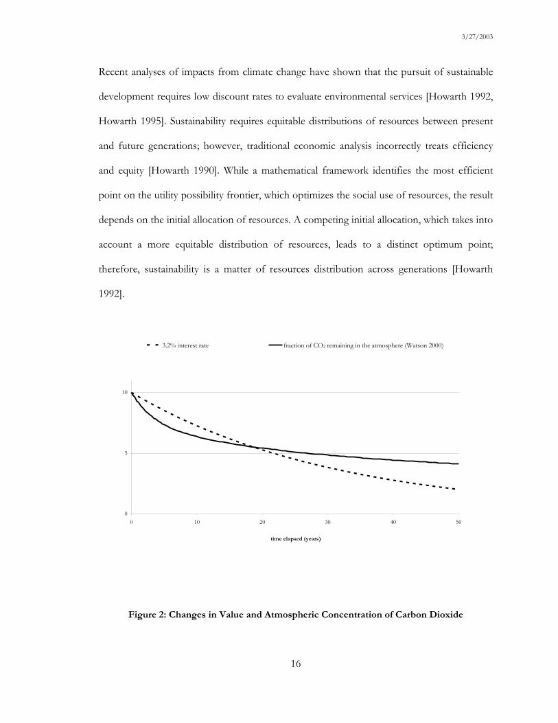
analysis over a 30 year period to 3.2% per year [OMB 2003]. Figure 2 shows the effects of
discounting over time using the discount rate prescribed by OMB and the persistence of
carbon dioxide in the atmosphere, represented by a parameterized function [Watson 2000].
In addition, one could argue that future pleasures are ethically equivalent to present pleasures
of the same intensity [Hotteling 1931]. Consequently, it would make sense to apply a zero
discount rate to run policy optimization models to reflect this postulate since future
generations are the ones who bear the costs of environmental degradation from climate
change.
3/27/2003
16
Recent analyses of impacts from climate change have shown that the pursuit of sustainable
development requires low discount rates to evaluate environmental services [Howarth 1992,
Howarth 1995]. Sustainability requires equitable distributions of resources between present
and future generations; however, traditional economic analysis incorrectly treats efficiency
and equity [Howarth 1990]. While a mathematical framework identifies the most efficient
point on the utility possibility frontier, which optimizes the social use of resources, the result
depends on the initial allocation of resources. A competing initial allocation, which takes into
account a more equitable distribution of resources, leads to a distinct optimum point;
therefore, sustainability is a matter of resources distribution across generations [Howarth
1992].
Figure 2: Changes in Value and Atmospheric Concentration of Carbon Dioxide
0
5
10
0 10 20 30 40 50
time elapsed (years)
3.2% interest rate fraction of CO2 remaining in the atmosphere (Watson 2000)

3/27/2003
17
Concerned with equitable welfare distribution, Howarth and Norgaard built an overlapping
generation model to illustrate that initial property rights determine the equilibrium and
distribution of welfare in a market economy. In their model, consumption and investment
levels are controlled by two generations that overlap, that is, old individuals of the earlier
generation and young individuals of the next generation live part of their lives together. In
addition, they assume that GHGs, which are associated with energy use in the economy,
have a negative impact on production [Howarth 1992]. Other ordinary economic
assumptions are made, such as diminishing marginal utility across all consumption goods,
and positive marginal time preference. Besides, the government operates capital transfers
between generations, which allow equitable welfare distribution and sustainable development.
Consequently, the equilibrium of the model and the value of all variables are function of
transfers between generations. The result is that the more assets are transferred to the next
generation, the lower is the discount rate; moreover, higher values are assigned to
environmental services. In short, they prove within the economic framework that the
adoption of low interest rates is part of a value judgment concerning an equitable
distribution of welfare between generations, and not an issue of pure mathematical efficiency
[Howarth 1998].
In summary, long time scales associated with climate change make discounting critical and
the literature shows that lower rates, which give more weight to long term benefits should be
considered. However, there is still no consensus on long term discount rates, even if it is
accepted that they should be distinguished from private market discount rates [Metz 2001].
3/27/2003
18
2.2.1.2 Economic Valuation
The second problem associated with economic impact valuation is the quantification of
climate change impacts or how changes in the concentration of GHG in the biosphere are
translated into socioeconomic impacts. The use of economics presupposes that we know the
value of environmental services now and in the future, which are either already incorporated
in the market or are converted into monetary values by the person in charge of the BCA.
The assertion that from economic perspective sustainability is a matter of intergenerational
equity is based on the assumption that values and preferences don not change over time,
which is not the case. Personal and societal choices are dynamic and something that is
accepted today may not be tolerated in the future.
Nonetheless, international development agencies are addressing sustainability through
environmental valuation [Howarth 1992]. In the case of climate change assessment,
environmental valuation requires a chain of steps beyond the assessment of the
correspondent GWP, and involves information acquisition, modeling, and evaluation.
Consequently, decision-making for climate change requires knowledge on a chain of issues
that finally are compared on a common basis. Usually, the conversion of a comprehensive
set of knowledge into money is difficult and several considerations are left aside during this
process.
Further, long time scales intrinsic to climate change cause unpredictable impact evaluations.
For instance, climate impacts will be imposed on future generations on different
communities with different value systems compared to values pertaining to present
evaluators. In economic terms this could mean variations in the elasticity of utility with
3/27/2003
19
respect to consumption and income [Schelling, 1995]. Consequently, it is possible that
adverse climate impacts in the future will be incommensurable based on monetary
compensations established in the present. Moreover, outcomes valued as benefits may be
challenged depending on who benefits from such outcomes. In short, it is unlikely that we
can be completely successful assigning money values to climate change impacts [Bradford
1999].
A BCA of climate change impacts is usually conducted based on top-down models of the
energy socioeconomic system [Bruce 1996], and balance marginal costs of climate change
mitigation against marginal benefits from avoided emissions. The same economic rationale
could be extended to the assessment of different electricity production options; that is,
alternatives would be compared through the quantification of the socioeconomic impacts
produced by each one. Nevertheless, it would be still necessary to rely on economic
evaluations of hard to value impacts, and heterogeneity in time and space could make the
analysis impossible.
Flaws in the economic analysis led to models that evaluate electricity sources independently
of environmental economic evaluations, and the pros and cons of alternative institutions for
the attainment of consensual environmental obligations have become more and more
accepted [Howarth 1990].
As a result, it could be more appropriate to use alternative physical units in environmental
assessments, which represent concentration of pollutants as the unit of analysis [Nyborg
2000]. The choices of physical units to compare alternatives is interesting because they are a
more direct result from scientific assessment models and bypass problems associated with
the economic quantification of the final impacts.
3/27/2003
20
One environmental evaluation method that uses this type of correlation is the intake fraction
method [Bennett 2002]. The idea is that the risk posed by pollution is assessed through the
fraction that is inhaled by a population living on a certain area over a given period of time
divided by the amount released at the source. One of the objectives of the intake fraction
method is to consolidate a consistent and transparent way to compare emissions-to-intake
studies performed by different researchers, helping the communication of the results.
The ecological footprint is another evaluation method that also follows the rationale of
correlating causes and consequences through a non monetized indicator. The method’s goal
is to find out how much land is necessary to support various human activities [Rees 2003].
Everyone has an idea about land dimensions, and therefore, one of the method’s strengths is
that the magnitude of the results is easily communicated even to lay people. Another
similarity between the GWE and the ecological footprint is that it was proposed as an
alternative to economists’ argument that the idea of carrying capacity is irrelevant to our
society. Instead of asking the question: how many people can be supported by a given land
area? The ecological footprint seeks the opposite: how much land is needed to support a
given population? The calculation of the footprint is based on the continuous supply and
assimilation of all the resources demanded by a stipulated population.
In the same vein of reasoning, the framework proposed in this work uses GWE as an
indicator, without incurring into the evaluation of actual socioeconomic and detailed
environmental impacts. As other studies it assumes that more GWE harms earth’s economy.
[Howarth 1990, Nordhaus 1999].
On the one hand, if an intermediate indicator such as GWE does not address the non
linearity between temperature changes and climate change impacts and costs, and may only

3/27/2003
21
become valuable after the establishment of links in the chain of consequences which goes
from emissions to atmospheric concentrations, climate forcing, changes in climate
parameters (such as global average surface temperature), climate change impacts, and finally,
economic costs of climate change damages [Shackley 1997, Smith 2000, O'Neill 2000]; on
the other hand, the use of GWE decoupled from ultimate damages of climate change could
benefit its applicability since less assumptions and uncertainties are incorporated in the
assessment, and besides they can be more clearly presented to a broad audience. Moreover,
GWPs are intended for use in studying relative rather than absolute impacts of emissions,
and correspond to specific time horizons [Houghton 2001]. The same idea is extended to the
use of GWEs.
Despite these two sorts of problems (discounting and valuation) related to the calculation of
benefits and costs associated with climate change outcomes and policies, a BCA of climate
change impacts favors climate stabilization over a business as usual scenario [Horwarth
2003], which makes eminent the need for actions to reduce current GHGs emissions.

3/27/2003
22
Chapter 3: Assessment Method and Approach
The framework used in this work is supported by the idea that climate change is a global
problem, and therefore, there is no need to assess regional and local impacts of climate
change if alternatives are scrutinized based on global compromises. However, this approach
does not deny the legitimacy of regional/local assessments of other sorts of problems; even
if it is conclusive when climate change impacts are at stake.
One advantage of the GWE method is its flexibility to accommodate different analytical
periods for the comparison of the alternatives. As a result, in the analysis the lifetime for
each electricity generation technology may be extended through routine maintenance,
retrofits, and upgrades following the idea that obsolescence is also dictated by social factors
[Lemer 1996].
The GWE method combines two well established methods LCA and Global Warming
Potential (GWP) and is discussed below.
3.1 The Global Warming Effect (GWE) Method
The quantification of the GWE for each facility is obtained through a hybrid LCA that
draws both on process based LCAs and economic input-output based LCAs and combines
the advantages of both methods. The input-output data are obtained from a model of the
U.S. economy developed by a team of researchers at Carnegie Mellon University – EIO-
LCA [Hendrickson 1998]. In the case of fossil fueled power plants information from the U.S.
3/27/2003
23
Energy Information Administration (EIA) was used to find out fuel consumption rates and
emission factors during the operation of the facilities.
The first step to assess GHG emissions from the construction of the power plants is to
identify the major energy and materials consumed by each facility and how much is
consumed over its life-cycle. This step parallels the inventory phase of the SETAC LCA, and
the information used is usually available in construction contracts and various published
sources, as noted throughout this work.
The EIO-LCA method was used to estimate the mass (M) of each GHG emissions (CO2,
CH4, N2O) from constructing and operating power plants based on the amounts and costs
of the materials and energy inputs. The construction assessment included material
(extraction, processing, and transportation) and energy (extraction/generation, processing,
and transportation) inputs, and equipment use in construction activities (fuel combustion).
For the operation stage of the fossil fueled power plants, fuel inputs are quantified in each
year of the service life, and air emissions are estimated from the fuel extraction,
transportation, and combustion phases.
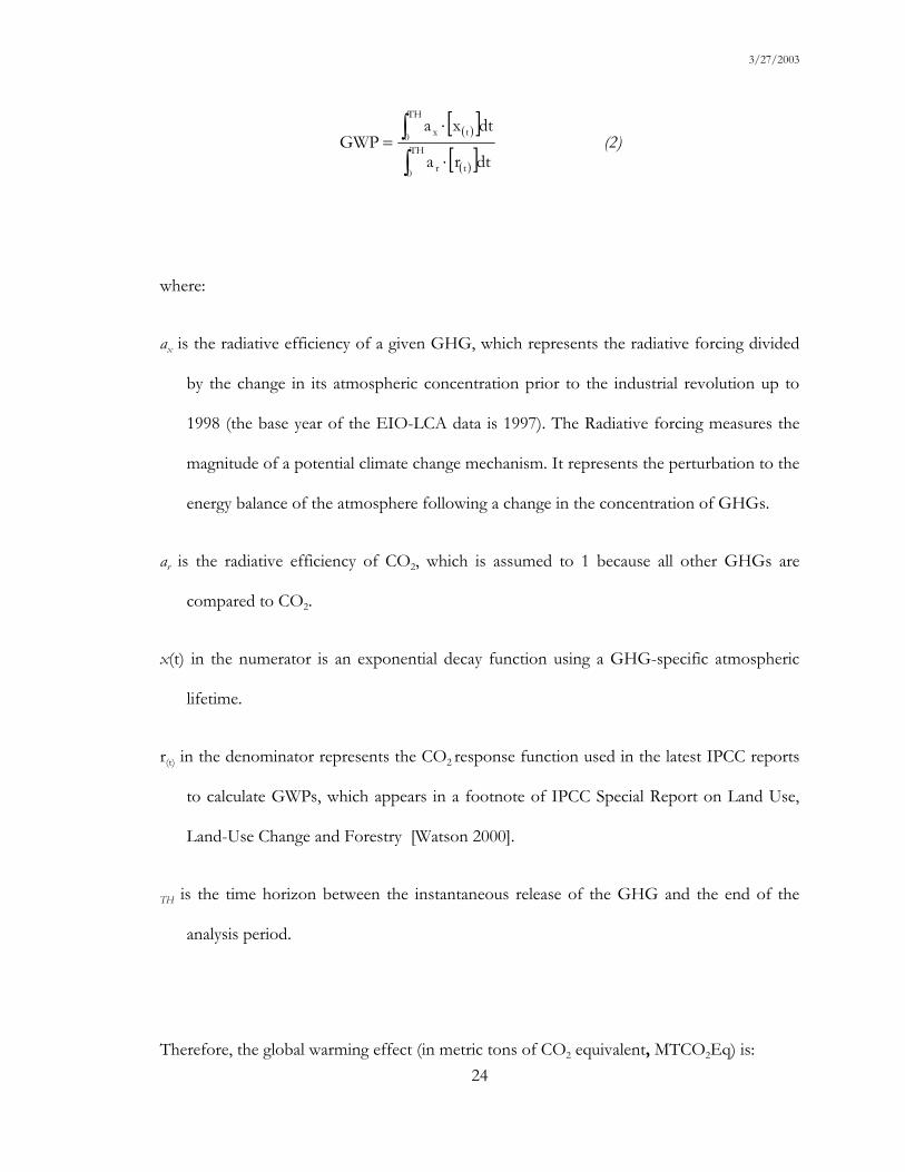
The effects of different GHGs on climate change are determined using the Global Warming
Effect (GWE), which is the sum of the product of instantaneous GHG emissions (M) and
their specific time-dependent GWP. The GWP for a GHG and a given time horizon is
[Houghton 2001]:
3/27/2003
24
( )[ ]( )[ ]∫
∫⋅
⋅= TH
0 tr
TH
0 tx
dtra
dtxaGWP (2)
where:
ax is the radiative efficiency of a given GHG, which represents the radiative forcing divided
by the change in its atmospheric concentration prior to the industrial revolution up to
1998 (the base year of the EIO-LCA data is 1997). The Radiative forcing measures the
magnitude of a potential climate change mechanism. It represents the perturbation to the
energy balance of the atmosphere following a change in the concentration of GHGs.
ar is the radiative efficiency of CO2, which is assumed to 1 because all other GHGs are
compared to CO2.
x(t) in the numerator is an exponential decay function using a GHG-specific atmospheric
lifetime.
r(t) in the denominator represents the CO2 response function used in the latest IPCC reports
to calculate GWPs, which appears in a footnote of IPCC Special Report on Land Use,
Land-Use Change and Forestry [Watson 2000].
TH is the time horizon between the instantaneous release of the GHG and the end of the
analysis period.
Therefore, the global warming effect (in metric tons of CO2 equivalent, MTCO2Eq) is:
3/27/2003
25
GWE = Σ Mj . GWPj, TH (3)
where:
Mj is the amount in metric tons of the instantaneous emission of each GHG “j”
GWPj, TH is the global warming potential for each GHG “j” calculated using equation (2)
For example, the GWE of CH4 emissions over 20 years is equal to the amounts of releases
in years 1, 2, 3, …20 multiplied by methane’s GWPs when the TH is 20, 19, 18, …1 years and
summed for the total. In the case of a emission that is constant every year there is no need
for the calculation of GWPs, and only the calculation of a GWP corresponding to the total
time period multiplied by the annual emission gives the radiative forcing produced by the
annual release of the GHG. However, if emissions vary from year to year then the
calculation of specific GWPs is necessary.
Therefore, the global impact of each technology over time is a function of the fraction of gas
remaining in the atmosphere in the future compared to the effect of CO2. In addition, in the
case of CH4, it is assumed that after atmospheric decay, all CH4 oxidizes into CO2, which is
not included in the GWP calculations for CH4, and thus is accounted for as additional CO2
[Houghton 2001]. The CO2 response function is used to determine the future concentration
of carbon in the atmosphere. The life time of a facility depends on the obsolescence of its
structures and technology. Consequently, the analysis periods depend on upgrades, changes
in technology, human values, resource availability, etc.
3/27/2003
26
According to the GWE the temporal scale of emissions is more important than their spatial
distribution, and the method captures this component very well. Another advantage of the
method is that it works with relative comparisons instead of the ultimate/absolute impacts
because it is based on GWP computations that compare the effect of GHG emissions to the
emission of a similar amount of CO2 over a chosen time horizon [Houghton 2001]. The
choice of an intermediate indicator to compare alternatives is interesting because it
eliminates the problems associated with the quantification of the final impacts caused by
climate change and provides a standardized method to compare alternatives [Lenzen 2002].
Such characteristics are also present in other environmental evaluation methods such as the
intake fraction method [Bennett 2002]. The final result of the assessment is a ranking of the
compared alternatives according to their GWE, which is a relative measure with no
compromise with the absolute impacts of each alternative.
3.2 Problems and Uncertainties Associated with the Assessment
Method
Because the framework combines two methods it also adds the problems from each one.
Besides that, there are also problems with the characterization of comparable power plants
to produce electricity. Thus, problems with the method are classified in three categories:
1. Problems associated with the LCA method
2. Problems associated with the GWE (GWP) method.
3. Problems associated with dimensioning of power plants according to site
specific characteristics and technological options.

3/27/2003
27
3.2.1 Problems with LCA
The LCA method used in the GWE assessment entails different problems. Some of these
problems have been already characterized as uncertainties in input-output analysis [Lenzen
2001]. While some of these problems may be characterized within a range of variable known
values and analytical choices, others go beyond this characterization and add uncertainty to
the assessment. Figure 3 presents a classification of problems within the LCA method. Four
main categories are proposed: data, temporal constraint, economic boundary, and
methodological constraint.
Data problems arise during data collection and interpretation. Problems such as incomplete
data and missing data are recognized by the EIO-LCA team.
“Incomplete data: While the eiolca.net strives to include
comprehensive data, some sources are incomplete. For example, the toxics
release inventory only is required for some industrial sectors and only for
plants above administratively defined threshold sizes. As a result, the
toxics emissions are likely to be underestimated.
Missing data: The eiolca.net software does not include all
environmental effects. For example, habitat destruction for
manufacturing plants is not included. Similarly, the external costs of
production are limited to health effects of conventional air emissions due
to lack of data on the valuation of other effects.” [EIO-LCA 2000].

3/27/2003
28
Sources of problems Temporal constraint
Data
Methodological constraint
Economic boundaryImported goods
Indirect outcomes
Constant technology
Constant returns to scale
No substitution effect
Old data
Collection
InterpretationInaccuracy
Incomplete data
Missing data
Other assumptions
Intra-sectoral resolution
National averages
Inventory method
Price based flows
Figure 3: Problems with LCA
While coping with incomplete data is beyond the capacity of the EIO-LCA team who works
with various self-reported public datasets, missing data limitation is also a question of
preferences. That is, the stressors selected to portray the environmental burden of products
and processes depend on how such stressors are valued by the analysts.
It is difficult to provide exact information on the accuracy of data sets; however, it is
possible to estimate basic standard errors for the elements of all basic input-output tables
based on the knowledge of the survey data sources [Lenzen 2001]. Although precautionary

3/27/2003
29
steps are taken during collection, processing, and tabulation of the data to reduce errors in
the U.S. economic census, no direct measurement of the error is made [U.S. Census 2003].
Data interpretation is also a problem in generic LCA methods. This problem spans from
measurements at the emitter level up to the information treatment at the analyst level. That
is, the emitter may not report all the emissions that are released by its activity or two analysts
may use divergent conversion factors to transform economic values into physical units that
generate conflicting outcomes. For example, the average real price of coal ($ per short ton)
delivered to electric utilities has decreased 32% between 1991 and the year 2000 (Real prices
are in 1996 dollars, calculated using implicit Gross Domestic Product price
deflators. Average prices are based on the cost including insurance and freight) [EIA 2002].
If someone uses the 2000 price to find out the amount of coal consumed by the electric
utilities in the U.S. in 1996 it results in a value 32% higher than the actual value. Conversely,
if someone uses a price higher than the actual price she underestimates the amount of coal
consumed. Consequently, all major assumptions involved in the preparation of the emission
factors per dollar of output for each sector should be disclosed so that the user traces back
parameters, and estimates the effect of alternative assumptions on the final emission factors.
The input-output method is also constrained by time. The data are specific to a given year,
and it takes sometime to tabulate 500 by 500 data tables for the whole U.S. economy.
Therefore, it is likely that data are outdated in comparison with the information required as
part of the analysis. Usually, input-output tables available from the U.S. Department of
Commerce are published with a 5 year delay. In addition, there is a lag in data supply from
environmental agencies as well [EIO-LCA 2000]. Consequently, recent technological
changes are not captured by input-output methods. Although some sectors are quite stable
3/27/2003
30
in terms of technological innovation, other sectors change more rapidly. One example is
water consumption data that was last time reported in 1982. Meanwhile, end-use water
technologies for different sectors have evolved leading to substantial water savings, even if
the economic output of the sector has grown over the same period [Gleick 2000].
Besides historical technological variability in the case of electricity production not only
power generation technology varies temporally but it also varies regionally because of the
diversity in terms of resources availability. In addition, depending of the scale of the “power
plant” the technology may be different. For example, solar energy may be harnessed by PV
modules at a small-scale level but it may be more appropriate to use a thermal solar electric
generator to produce power at a large-scale level [Kreith 1990].
Intra-sector resolution corresponds to the level of aggregation within a given sector. For
example, the sector “Turbine and Generator Sets” encloses disparate sub-sectors such as:
• Gas turbines, mechanical drive
• Governors, steam
• Hydraulic turbines
• Solar powered turbine-generator sets
• Steam engines, except locomotives
• Steam turbines
• Tank turbines
• Turbine generator set units, complete steam, gas, and hydraulic
• Turbines steam, hydraulic, and gas-except aircraft type
• Turbo-generators
• Water turbines
3/27/2003
31
• Wind powered turbine-generator sets
• Windmills for generating power
Although they are all turbines and energy related the technology of a gas turbine is quite
different than the technology of a wind turbine. Even if EIO-LCA includes 500 sectors,
sometimes more detailed information on specific products or processes is needed. This
problem is classified under temporal constraints because usually the number of sectors, and
sometimes their classification, which are determined and reported by the U.S. Department of
Commerce, changes for each new report.
The use of an economic boundary yields limitations and advantages. A consequence of the
use of the national economy as a boundary is the lack of information on imported goods
[Lenzen 2001]. EIO-LCA assumes that imported goods are produced similarly to domestic
goods. Thus, if steel is used by a US company, the environmental effect of steel is expected
to be comparable to those made in the US. To the extent that overseas production is
regarded as more or less of an environmental concern, then the factors presented by EIO-
LCA should be adapted. For example, the energy efficiency index measures the energy input
necessary to produce a given amount of product. The more efficient the sector in a country,
the lower is its energy efficiency index. The best practice level selected as a marker
corresponds to 100% [Houghton 2001]. In the case of steel, for example, it is known that
the energy efficiency index in the U.S. is higher than several exporting countries (figure 4).
Thus EIO-LCA overestimates life-cycle energy consumption if imported steel is used in the
manufacturing of a good in the U.S.
The aggregate energy efficiency index (EEI) is calculated as:
EEI = (Σi Pi· SECi)/( Σi Pi· SECi,BP) (4)

3/27/2003
32
Where:
Pi is the production volume of product “i”;
SECi is the specific energy consumption for product “i”;
SECi,BP is a best-practice reference level for the specific energy consumption for product “i”.
By applying this approach a correction is made in order to account for structural differences
between countries in each of the industrial sectors considered. A typical statistical
uncertainty for these figures is 5% but because of statistical errors higher uncertainties may
occur in individual cases.
Another problem that affects EIO-LCA is that indirect outcomes and their respective
environmental burden are not always included in the analysis. For instance, if the method is
used to assess carbon dioxide emissions from a labor intensive process, and most of the
employees of the firm spend a long time commuting back and forth to their work.
Emissions from employee's automobiles are not included because the fuel is purchased with
their salaries, and such economic transaction is exogenous to the industrial process assessed
by EIO-LCA. Therefore, if the transportation of employees represents a considerable
amount of pollution, it is ignored by the method. A way to correct such discrepancy would
be to find out how much labor is associated with the production of the commodity and
combine such value with travel distance, per capita fuel consumption, carbon content in the
fuel, carbon dioxide airborne fraction, etc.

3/27/2003
33
Figure 4: Energy Efficiency Index for Iron and Steel Production [Metz 2001].
Because only commodities used in the fabrication of other commodities or services are
captured in input-output methods some consequences associated with other phases of the
life-cycle of a product may be ignored. For example, the end of life of a product may entails
serious impacts that need to be quantified separately [Lenzen 2001].
A similar problem, which also ignores part of the impacts posed by a product or activity,
spawns from the inventory method applied to identify emissions. Indeed, it is hard to be
comprehensive and identify all emission sources for a given compound, therefore, only the
major ones should be pursued but sometimes it is very difficult to quantify major GHG
emissions associated with human activities. For example, nitrous oxide emission estimations
in EIO-LCA are based on the assumption that 10% of the oxides of nitrogen (NOx)
emissions are converted to nitrous oxide (N2O) [EIO-LCA 2000]. Oxides of nitrogen
emissions are reported by the U.S. U.S. EPA based on fuel consumption [U.S. EPA 2002].
3/27/2003
34
However, it is recognized that a more significant amount of anthropogenic N2O comes from
agricultural soils [Houghton 2001]. Actually, over 65% of atmospheric N2O comes from soil
as a result of nitrification and denitrification [Bouwman 1990]. Therefore, if there is a
concern with nitrogen oxides emissions it makes sense to identify the area of crops which
are necessary to sustain a given industrial activity and the effects of cultivation practices on
the balance of nitrogen between soil and air.
Constant returns to scale and the inability to substitute inputs in a given process are amongst
the most well known limitations of input-output analysis [Levinson 1979]. The constant
returns to scale assumption means that given the resources needed to produce one unit of a
given commodity, it is just a matter of scaling up these amounts to find out how much is
necessary to produce 1,000 units. However, if a manufacturer faces increasing returns to
scale, that is, the larger is its total output, less input is demanded per unit of output, such
efficiency gains are not captured by EIO-LCA.
Substitution effects do not fit in the EIO-LCA method as well. if we consider the example
of a producer that faces high electricity costs and decides to build its own wind power plant,
and we are concerned with the level of emissions associated with its final product, then, we
should consider the effects of the substitution of grid electricity for self-supply power
because electricity generated by different systems is likely to produce different air emissions.
In the case of input-output based LCA, the use of emission factors in a different region
should take into account carbon dioxide intensities pertaining to the electricity generation
mix in that region [Lenzen 2002].
In addition, EIO-LCA method represents all transactions within the U.S. economy, and
aggregates singular performances within the same sector. Consequently, EIO-LCA
3/27/2003
35
indicators represent the average performance of a myriad of producers within a sector. On
the one hand, the use of such values could require some adjustments to become more
precise, on the other hand, they are opportune to assess generic projects and products within
a given sector and hold comparisons based on the relative effect of alternative options.
Moreover information from the EIO-LCA database is readily available and free.
Finally, the characterization of physical flows through the input-output method is based on
money flows. The problem is that prices vary both over temporal and spatial scales, and
therefore, proportionality between prices and physical quantities does not hold. Prices for
the same good are also different depending on the consumer (consumer discrimination). For
example, electricity in the same region and at the same moment can be sold at different
prices for industrial and residential consumers [Lenzen 2001].
A methodological distinction when doing a LCA is the difference between choices and
uncertainty. While some criteria applied to the analysis are to the discretion of the analyst,
others reflect the incomplete knowledge about the true value of a parameter. An imprecise
measurement aggregates uncertainty to the analysis in the same way that estimations of
parameters that are difficult to assess with precision also constitute a source of uncertainty.
Although sometimes the analyst is forced to assume some values for parameters that are not
precisely defined, this practice is completely different than ignoring something that is known
or selecting alternatives among a set of available possibilities.
Only when the range of uncertainty is know or at least a given distribution can be associated
with this range it is possible to use some computational frameworks to analyze the
consequence of such variability in the final results of the assessment. Monte Carlo simulation
3/27/2003
36
is an alternative to cope with uncertainties that propagates known parameter fluctuations
into an uncertainty distribution of the output variable.
Monte Carlo simulation is used to reveal the effects of uncertainties in the final results,
which requires the selection of specific statistical distribution functions for the uncertain
parameters. The logical association of the parameters is also selected by the analyst and the
output of the simulation produces a range of possible scenarios. A sensitivity analysis
targeting parameters independently can be used to find out which parameters pose the
greatest effect on the final results.
3.2.2 Problems with the Global Warming Potential (GWP)
The GWE draws on the climate sensitivity parameter that is proposed based on the
relationship between the effects of changes in GHGs concentrations on the global average
temperature. The scientific basis of the GWE is the same behind the GWP, and therefore,
problems associated with the GWP also manifest with the use of the GWE.
The use of GWPs is challenged because they are not able to capture all the complexity
inherent to the global climate system. Changes in ice cover and land use, which affect the
albedo, are left aside, sea level changes are left aside, precipitation changes are left aside, and
natural phenomena such as the action of volcanoes and changes in solar incoming radiation
are left aside (Figure 5). Besides all these external sources of problems there are also some
problems inherent to the GWP formulation.
The calculation of global warming potentials comprises five parameters. The first is the
choice of the time horizon, which is driven by the goals of the analysis. The time horizon is
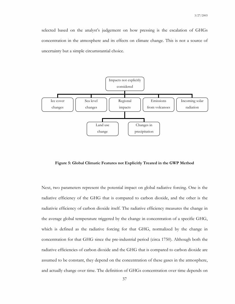
3/27/2003
37
selected based on the analyst’s judgement on how pressing is the escalation of GHGs
concentration in the atmosphere and its effects on climate change. This is not a source of
uncertainty but a simple circumstantial choice.
Figure 5: Global Climatic Features not Explicitly Treated in the GWP Method
Next, two parameters represent the potential impact on global radiative forcing. One is the
radiative efficiency of the GHG that is compared to carbon dioxide, and the other is the
radiativie efficiency of carbon dioxide itself. The radiative efficiency measures the change in
the average global temperature triggered by the change in concentration of a specific GHG,
which is defined as the radiative forcing for that GHG, normalized by the change in
concentration for that GHG since the pre-industrial period (circa 1750). Although both the
radiative efficiencies of carbon dioxide and the GHG that is compared to carbon dioxide are
assumed to be constant, they depend on the concentration of these gases in the atmosphere,
and actually change over time. The definition of GHGs concentration over time depends on
Impacts not explicitly
considered
Ice cover
changes
Sea level
changes
Regional
impacts
Emissions
from volcanoes
Incoming solar
radiation
Land use
change
Changes in
precipitation

3/27/2003
38
future scenarios that involve a set of independent variables such as: energy policy (what are
the future energy sources: fossil or renewables?), economic growth, population growth,
technology (what electricity supply options will be available in the future?), etc. Accordingly,
the radiative forcing of GHGs is also affected by the outcomes of the models used to
calculate the atmospheric concentrations of the GHGs and the consideration of chemical
reactions between different compounds in the atmosphere.
Finally, the last two parameters represent the residence time of carbon dioxide and the other
GHG in the atmosphere. The turnover time of GHGs depend on mechanisms and
feedbacks that are not precisely modeled; in addition, in the case of carbon dioxide,
prognoses of future atmospheric concentrations are affected by the global carbon cycle
model used to calculate future CO2 concentrations, and concurrent carbon models present
different degrees of complexity [Oeschger 1983].
In summary, the GWP is an index used to compare the relative importance of different
GHGs in terms of they climate forcing. The numeraire for the GWP is the forcing of carbon
dioxide integrated over the period of analysis, which corresponds to the effect of a given
amount of carbon dioxide released to the atmosphere on the global mean temperature
[Houghton 2001]. This value is the denominator of the GWP formula (2) and is obtained
through the product of the remaining concentration of carbon dioxide in the atmosphere
times its radiative efficiency. Therefore, two basic parameters in the GWP method are the
radiative efficiencies and the factors affecting the balance of GHGs in the atmosphere.
3/27/2003
39
3.2.2.1 Problems with Radiative Efficiency
The radiative efficiency is the radiative forcing normalized by the change in concentration of
the species of interest, which are usually well mixed gases. Well mixed gases such as CO2,
CH4, and N2O are characterized by residence times long enough to remain well mixed in the
troposphere. The radiative forcing concept is consistent with the assumption that there is a
relationship between the global average forcing and the global average temperature.
Accordingly, the radiative forcing denotes an externally imposed perturbation, natural or
anthropogenic in the radiative energy budget of the earth’s climate system. One example of a
natural perturbation are emissions from volcanoes that are estimated as 0.02 to 0.05 Pg C yr-1
Anthropogenic or human perturbations have been much more significant over the last 100
years and include fossil fuel burning (6.3 Pg C yr-1) and land-use change [Houghton 2001].
Nevertheless, these two sources of carbon contribute to the increase in carbon dioxide
concentration in the atmosphere and equally contribute to an increase in the global radiative
forcing of the earth.
The adjective radiative is used because the idea is similar to the assessment of radiation from
the decay of different radioactive substances that generate compounds, each one with
different characteristics (life-time and radioactive emissions) and responsible for a certain
share of the total radiation produced [Smith 1993]. A parallel idea holds for the effect of
different GHGs on the global climate. That is, the radiative forcing of species with
characteristic residence times in the atmosphere is combined in a global radiative forcing.
The climate sensitivity parameter (λ) measures the ratio between the global mean
temperature response (∆T) and the change in radiative forcing (∆F). It is a global parameter,
3/27/2003
40
and in current one-dimensional models, such as the old Arrhenius model [Arrhenius 1896], λ
is a almost constant for various radiative forcings and corresponds to 0.5 K/(Wm-2), which
denotes a possible universality for the relationship between forcing and global temperature
changes [Houghton 2001]. Such universality is a strong reason to take λ as a central element
in global climate models and define a set of possible outcomes such as changes in ice cover,
sea level, etc as functions of changes in raditive forcing, which implies a proportional change
in the global average temperature. The problem is the circularity in these definitions because
changes in ice cover should also affect the global forcing.
Error! Objects cannot be created from editing field codes.
(5)
Nevertheless, although the value for climate sensitivity varies across different models, within
each model it is found to be constant for a wide range of perturbations. Even more complex
models, which involve three-dimensional experiments, show that radiative forcing continues
to be a good estimator for global mean temperature changes.
“The invariance of λ has made the radiative forcing concept appealing as a convenient measure to estimate the
global, annual mean surface temperature response without taking the recourse to actually run and analyze,
say, a three dimensional Atmosphere-Ocean General Circulation Model (AOGCM) simulation”
[Houghton 2001]
Furthermore, different radiative forcing precursors are all assumed to affect the
global climate in the same way [Houghton 2001], and it is difficult to isolate the radiative
forcing due to one precursor within the set of possible components that affect the whole
system. Actually, other components besides GHGs also affect the global radiative forcing;
however, the current knowledge about their effects is still limited (Figure 6).

3/27/2003
41
Figure 6: Global and Annual Mean Radiative Forcing (1750 to present) [Houghton 2001].
Critics of GWPs highlight that global mean forcing estimates are not necessarily indicators
of the regional impacts of climate change. Actually, regional responses to variant forcings
can differ from homogeneous forcing responses, and changes in other parameters such as
ice cover, precipitation, land use change, and sea level, which are all related to global climate
change, are not included in radiative forcing formulations. Consequently, advocates of more
complex models rely on three-dimensional atmosphere-ocean general circulation models
(AOGCM) that are composed by three-dimensional atmospheric general circulation models
(AGCMs) integrated to ocean general circulation models (OGCMs), which include sea-ice
interactions and terrestrial models. The resolution of such models is much greater than the

3/27/2003
42
model used to calculate GWPs, and they allow the modeling of regional outcomes in a much
smaller scale.
In any case, climate change science is always evolving, and even the methods to calculate
radiative forcing are changing over time. Such changes, in part, attempt to internalize
knowledge based on the output from more complex models. In the IPCC 2001 report, the
CO2 radiative forcing, which corresponds to a doubling in the concentration of CO2 in the
atmosphere, ranges from 3.5 to 4.1 W m-2; and its variation since the pre-industrial era
corresponds to 1.46 W m-2 [Houghton 2001]. Such values are slightly different from the
previous IPCC report, and reflect the inclusion of stratospheric temperature adjustments and,
short wave forcing in the computations of radiative forcing. That is, even if the GWP does
not deal explicitly with a series of factors that affect the global climate, many of those
manifestations are included by changing the value corresponding to the radiative forcing of a
given GHG.
In addition, the radiative forcing of carbon dioxide is time dependent because it depends on
the current CO2 concentration in the atmosphere; thus different formulations have been
proposed to estimate the radiative forcing for CO2 based on its atmospheric concentration
(Table 1).
The first row in table 1 lists an expression with a form similar to Houghton (1990) but with
newer values for the constants. The second row is a more complete and updated expression
similar in form to that of Shi (1992). The third row expression is from WMO (1999), based
on Hansen et al. (1988). The symbol “C” is CO2 in ppm, and the subscript “0” denotes the
pre-industrial concentration, which is assumed to be 278 ppm in the year 1750 [Houghton
2001]. The constant in the simplified expression on the first row is based on radiative
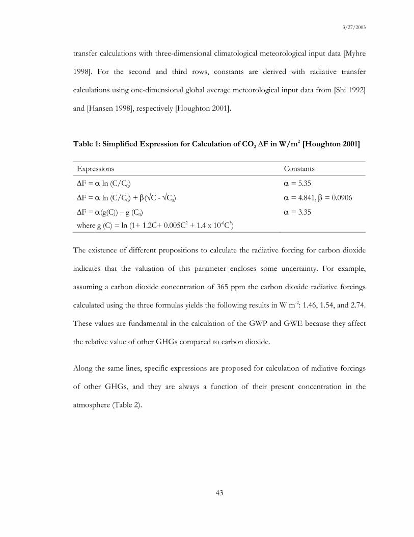
3/27/2003
43
transfer calculations with three-dimensional climatological meteorological input data [Myhre
1998]. For the second and third rows, constants are derived with radiative transfer
calculations using one-dimensional global average meteorological input data from [Shi 1992]
and [Hansen 1998], respectively [Houghton 2001].
Table 1: Simplified Expression for Calculation of CO2 ∆F in W/m2 [Houghton 2001]
Expressions Constants
∆F = α ln (C/C0)
∆F = α ln (C/C0) + β(√C - √C0)
∆F = α(g(C)) – g (C0)
where g (C) = ln (1+ 1.2C+ 0.005C2 + 1.4 x 10⁻⁶C3)
α = 5.35
α = 4.841, β = 0.0906
α = 3.35
The existence of different propositions to calculate the radiative forcing for carbon dioxide
indicates that the valuation of this parameter encloses some uncertainty. For example,
assuming a carbon dioxide concentration of 365 ppm the carbon dioxide radiative forcings
calculated using the three formulas yields the following results in W m-2: 1.46, 1.54, and 2.74.
These values are fundamental in the calculation of the GWP and GWE because they affect
the relative value of other GHGs compared to carbon dioxide.
Along the same lines, specific expressions are proposed for calculation of radiative forcings
of other GHGs, and they are always a function of their present concentration in the
atmosphere (Table 2).

3/27/2003
44
Table 2: Simplified Expression for GHGs ∆F calculations in W/m2 [Houghton 2001]
Trace gas Expressions Constants
CH4 ∆F = α(√M - √M0) – (f(M,N0) – f(M0, N0)) α = 0.036
N2O ∆F = α(√N - √N0) – (f(M0,N) – f(M0, N0)) α = 0.12
CFC-11 ∆F = α(X – X0) α = 0.25
CFC-12 ∆F = α(X - X0) α = 0.32
The expression on the third row in table 2 is used for all CFCs and CFC replacements, but
with different values for α i.e., the radiative efficiencies. The subscript “0” denotes the
unperturbed concentration (pre-industrial), and the function used in rows 1 and 2 is:
f(M,N) = 0.47 ln[1+2.01x10⁻⁵ (MN)0.75+5.31x10⁻¹⁵ M(MN)1.52] (6)
Where:
M is CH4 in ppb
N is N2O in ppb
X is CFC in ppb
Although the total climate feedback is treated as being invariable for the homogeneous
global system, individual feedbacks have different strengths. Besides direct effects some
compounds modify the radiative balance through indirect effects relating to chemical
transformations or change in the distribution of other active species. This calls for
adjustments on radiative forcings depending on the understanding of their stocks and flows
in the atmosphere.
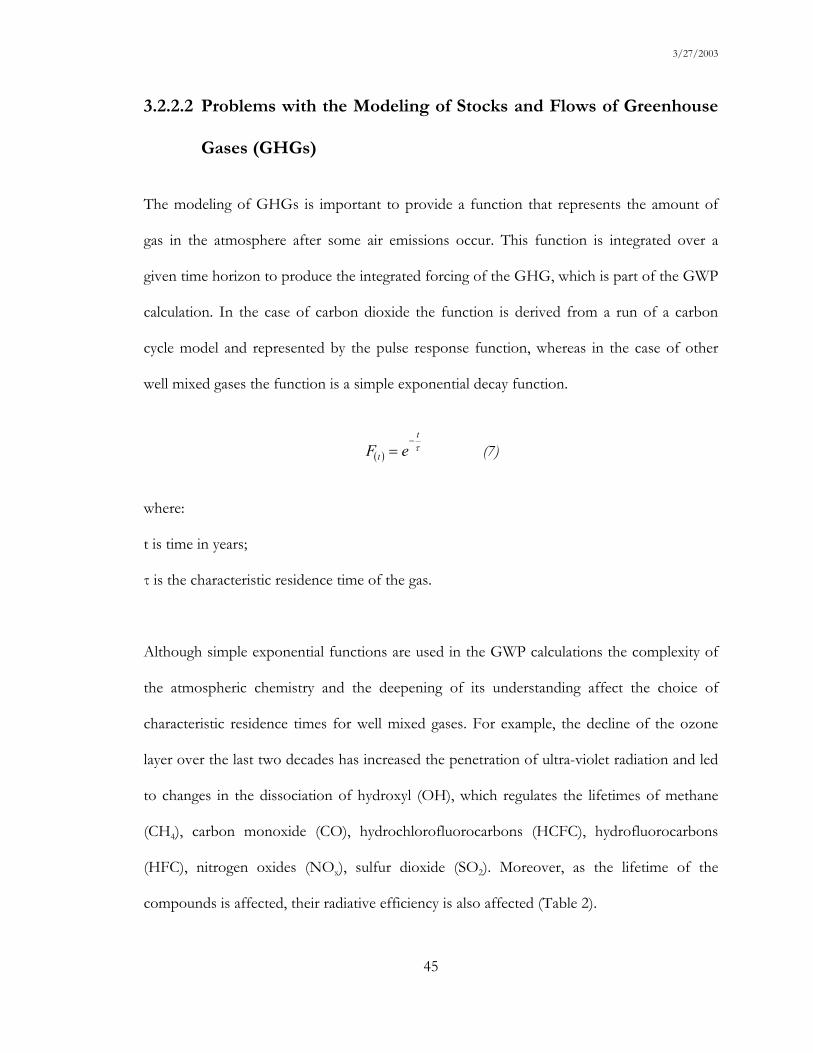
3/27/2003
45
3.2.2.2 Problems with the Modeling of Stocks and Flows of Greenhouse
Gases (GHGs)
The modeling of GHGs is important to provide a function that represents the amount of
gas in the atmosphere after some air emissions occur. This function is integrated over a
given time horizon to produce the integrated forcing of the GHG, which is part of the GWP
calculation. In the case of carbon dioxide the function is derived from a run of a carbon
cycle model and represented by the pulse response function, whereas in the case of other
well mixed gases the function is a simple exponential decay function.
( )τt
t eF−
= (7)
where:
t is time in years;
τ is the characteristic residence time of the gas.
Although simple exponential functions are used in the GWP calculations the complexity of
the atmospheric chemistry and the deepening of its understanding affect the choice of
characteristic residence times for well mixed gases. For example, the decline of the ozone
layer over the last two decades has increased the penetration of ultra-violet radiation and led
to changes in the dissociation of hydroxyl (OH), which regulates the lifetimes of methane
(CH4), carbon monoxide (CO), hydrochlorofluorocarbons (HCFC), hydrofluorocarbons
(HFC), nitrogen oxides (NOx), sulfur dioxide (SO2). Moreover, as the lifetime of the
compounds is affected, their radiative efficiency is also affected (Table 2).

3/27/2003
46
The lifetime of methane is also affected by several processes in the atmosphere. However,
most studies assume that its climate forcing remains constant within the foreseeable future
[Lelieveld 1993]. Industrial emissions, soil removal and chemical reactions in the biosphere
govern the lifetime of methane, and wetlands are a significant source of methane, which are
responsible for 23% to 40% of natural emissions. Reactions with hydroxyl (OH-) destroy
about 90% of the methane in the atmosphere [Lelieveld 1993], which then oxidizes into
carbon monoxide. Carbon monoxide has a residence time of months and is ultimately
converted to carbon dioxide [Crutzen 2001]. Therefore all CH4 emitted to the atmosphere
ultimately is converted to CO2.
Changes in scientific understanding affects the parameters used in GWP calculations. The
lifetimes of CH4 and N2O that were 12.2 and 120 years respectively in the 1995 IPCC report
[Houghton 1995] were adjusted to 12 and 114 years respectively in the 2001 IPCC report
due to feedbacks of emissions on lifetimes [Houghton 2001].
Although calculations involving CH4 mixing ratios and its instantaneous forcing are subject
to assumptions and uncertainties, the IPCC 2001 report assumes that the radiative forcing
for CH4 is 0.49 W m-2, its pre-industrial concentration is 700 ppb, and its concentration in
1998 is 1,745 ppb [Houghton 2001]. However, the calculated radiative efficiency of methane
is 4.69 x 10⁻⁴ W m-2 ppb-1 and not 3.7 x 10⁻⁴ Wm-2 ppb-1 as indicated on table 6.7 of the same
report. The radiative efficiency of methane combined to its characteristic residence time, the
radiative efficiency of carbon dioxide, and the function representing the behavior of carbon
dioxide in the atmosphere plus a given time horizon are the five parameters used in the
calculation of GWPs for CH4. The CH4 GWP values reported in the third assessment report
TAR of the IPCC based on 20, 100, and 500 years are 62, 23, and 7, respectively.
3/27/2003
47
Beyond assumptions and uncertainties associated with methane, approaches to carbon
dioxide, which is the numeraire for GWP, are also controversial. For example, it is difficult
to establish a singular residence time for carbon dioxide in the atmosphere since this GHG
is not removed by chemical decay from the atmosphere and is constantly transferred to
different pools, which are regulated by different processes [Bruhl 1993, Lashof 1990, O'Neill
2000]. Carbon cycle models, which are the source for the parameterized pulse response
function (PRF) to calculate the integrated amount of carbon dioxide in the atmosphere over
time are discussed next.
3.2.2.3 Carbon Cycle Models and Pulse Response Functions (PRFs)
The utility of models rely on different kinds of calculations as a function of time. For
example, forward modeling involves the prescription of specific emission profiles (Q(t)) to
find out atmospheric concentration levels in the future whereas inverse modeling calculates
the emissions that lead to a given concentration level (C(t)). Another use of models is the
calculation of pulse response functions that are used in the calculation of GWPs.
The spectrum of climate change models is rich and stems from simple concentration
extrapolation models to atmosphere-ocean general circulation models (AOGCM). The
mechanics embedded in OGCMs is derived from fundamental physical and chemical
principles [Enting 1994]. Concurrent representations of the carbon cycle, which balance the
carbon budget over time, lead to different future atmospheric concentration levels for a
specific projection of future carbon emissions [Bruce 1996].
3/27/2003
48
Basically, global carbon cycles represent two types of forcings: anthropogenic forcing and
responses to such forcings, which feedback in the exchange rates between different boxes of
the model. Anthropogenic forcing results from GHG emissions due to fossil combustion,
and land use change. The response to such forcings reflects on changes in atmospheric
concentrations, carbon uptake by oceans and terrestrial ecosystems. The partitioning
between carbon dioxide uptake by oceans and land is not an issue that is already resolved
and remains a source of uncertainty in all proposed models independently of their resolution
or degree of complexity.
Terrestrial carbon models use discrete compartments that represent leaves, branches, litter,
roots, and soil carbon. Carbon is stored in each of these compartments and the turnover
time represents the amount of time that an atom of carbon stays in the compartment.
The atmospheric carbon budget as a function of time is represented by the following
equation that represents carbon flows [Enting 1994]:
)()()()()(123.2 tresidtferttoceantntfoss SSSDQCdtd
−−−+= (8)
where:
2.123GtC ppm-1 refers to the size of the atmosphere in moles times the mass of one mol
of carbon
C is the atmospheric CO2 concentration in ppm
Qfoss(t) is the fossil emission rate
Dn(t) is the net release from land use change
Socean is the net carbon uptake by the ocean
3/27/2003
49
Sfert is the net flux associated with higher CO2 concentrations
Sresid(t) is a residual term associated with neglected processes
In this formulation, anthropogenic forcing terms are composed of fossil fuel emissions
(Qfoss(t)) and net carbon releases from land use change Dn(t). Variations of the same
fundamental parameters are part of every modeling effort undertaken.
The High Latitude Exchange/Interior Diffusion Advection (HILDA) model used by the
IPCC for simulating the transport of CO2 between the ocean, the atmosphere and the
biosphere is the source for the PRF that is used in the calculation of the GWPs by the IPCC.
HILDA, which is also known as the Bern model has a structure with six boxes (Figure 7).
HILDA is already a parameterized model formed by simplified descriptions that are present
in more complex models. Six boxes are part of the model. One box represents the biosphere
or everything pertaining to the terrestrial ecosystem. Another box represents the atmosphere,
which corresponds to a layer with an average height of 12 km. Four boxes represent the
ocean that is differentiated according to different latitudes. Out of these four boxes two
represent the superficial layer up to 75 m deep, which is divided in low latitude (LS) and high
latitude (HS) boxes. The remaining 2 boxes represent the deep waters (3,800 m) and are also
divided according to their latitude. An advective circulation oceanic current and a depth
dependent eddy diffusion coefficient, which captures flows between each subjacent box, are
also part of the ocean model. Actually, the limiting process for carbon dioxide uptake by
oceans is the internal mixing in the ocean. Flows in the model represent the carbon exchange
between the boxes and affect the atmospheric concentration of CO2.
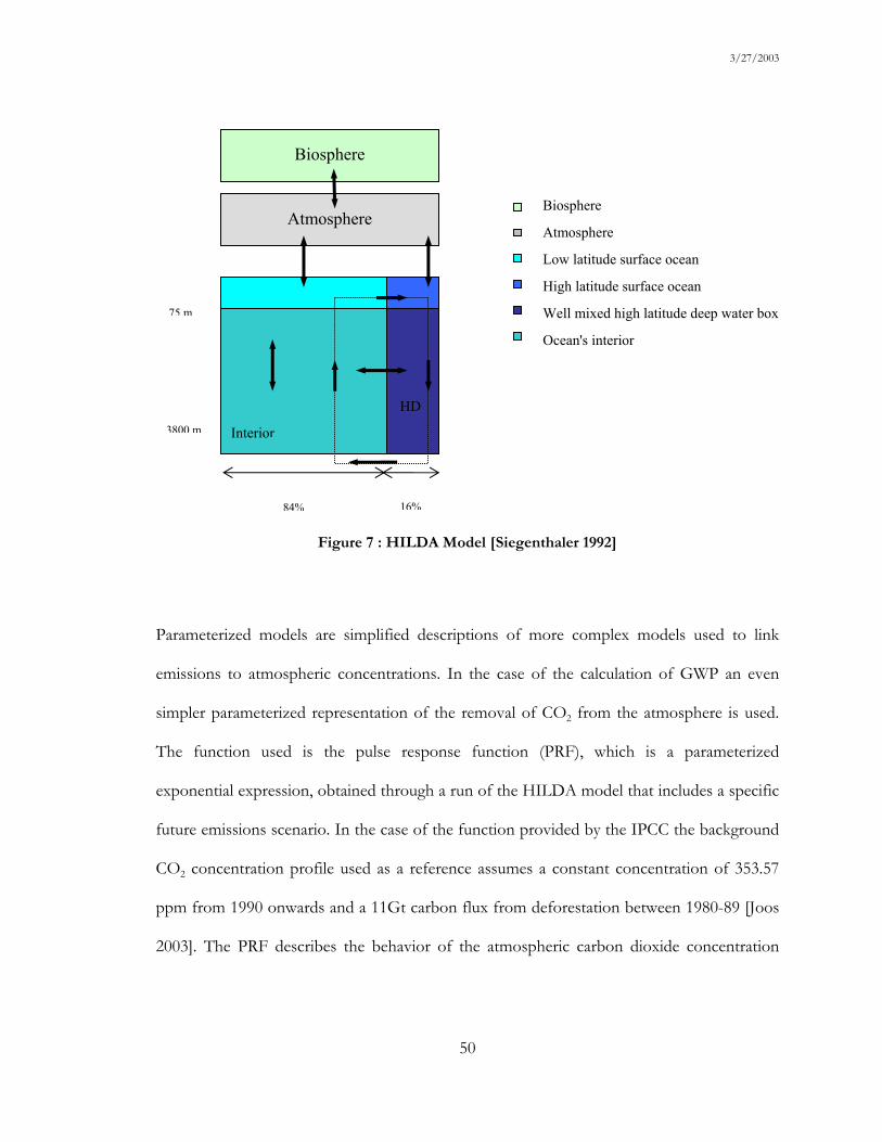
3/27/2003
50
Figure 7 : HILDA Model [Siegenthaler 1992]
Parameterized models are simplified descriptions of more complex models used to link
emissions to atmospheric concentrations. In the case of the calculation of GWP an even
simpler parameterized representation of the removal of CO2 from the atmosphere is used.
The function used is the pulse response function (PRF), which is a parameterized
exponential expression, obtained through a run of the HILDA model that includes a specific
future emissions scenario. In the case of the function provided by the IPCC the background
CO2 concentration profile used as a reference assumes a constant concentration of 353.57
ppm from 1990 onwards and a 11Gt carbon flux from deforestation between 1980-89 [Joos
2003]. The PRF describes the behavior of the atmospheric carbon dioxide concentration
Biosphere
Atmosphere
LS HS
HD
Interior
75 m
3800 m
84% 16%
Biosphere
Atmosphere
Low latitude surface ocean
High latitude surface ocean
Well mixed high latitude deep water box
Ocean's interior
3/27/2003
51
after a unique perturbation, which equals to 10 Gt of carbon injected in the atmosphere in
the year 1995.
Usually PRFs are obtained either assuming a background with zero emissions, which relates
to pre-industrial concentrations, or a background corresponding to emissions leading to a
given future stabilization level (353.57 ppm).
The response function Ga(t) is evaluated as [Enting 1994]:
F[CO2(t)] = 2.123[C(t) – Cb(t)]/10.0 (9)
Where C(t) is the concentration of carbon in the atmosphere and Cb(t) is the background
concentration, which depends on the future emission scenario selected. The factor 2.123
GtC ppm-1 is the size of the atmosphere (box) in moles times the molecular weight of
carbon.
The approximation of the output of the HILDA model, which is used in the GWPs
calculations for the 1995 and 2001 IPCC reports, corresponds to the following
parameterized response function [Watson 2000]:
F[CO2(t)] = 0.175602 + 0.137467e-t/421.093 + 0.185762e-t/70.5965 + 0.242302e-t/21.42165 + 0.258868e-t/3.41537 (9)
Where F is the fraction of CO2 remaining in the atmosphere and “t” is the time after the
pulse was emitted in years. This function is based on results running the HILDA model
assuming a background concentration of 353.57 ppm.
The pulse response function used in the denominator of the GWP depends on the results of
the carbon cycle model used to calculate the fate of carbon dioxide emissions in the
3/27/2003
52
atmosphere. Therefore, problems embedded in the carbon cycle model affect the
coefficients of the pulse response function, and a discussion on the choices and uncertainties
embedded in the model enhances the validity of the results obtained with the model.
Uncertainties in the model are classified in:
1. model error
2. imprecise calibration
3. budget uncertainty
The existence of different models demonstrates the existence of different model structures
and parameters. However, the variability amongst current models is not an indicator of the
actual uncertainty in the predictions. It is possible that a small group of models does not
capture the full range of uncertainty. Moreover, some key process could be missing in every
model [Enting 1994].
In a reasonable model the parameters used should be expected to hold in the future, and the
validation of carbon cycle models is fundamental to give credibility to the projections. One
concern is that different sorts of models would present different results if they run similar
input data. This has been dismissed by a recent comparison of two different models
predicting the future global climate [Zwiers 2002].
Uncertainties in predictions made with the model affect the PRF that already contains
uncertainty from its ability to represent in a single function actual observational data. The
estimation that the current CO2 concentration is growing at a rate of 3.2 ± 0.1 PgC yr-1
during 1990 to 1999 [Houghton 2001] reflects this kind of uncertainty. The variability in land

3/27/2003
53
and ocean uptake may explain why in 1992 the growth rate was 1.9 PgC yr-1 and in 1998 it
was 6.0 PgC yr-1.
The information used to calibrate the model needs to report both past carbon dioxide
concentrations in the atmosphere and emissions. Direct measurements of CO2 concentration
started in 1957 and to extend back the historical series of CO2 researchers rely on indirect
measurements based on physical and biophysical principles. For example, tree ring records,
corals, lake sediments, and ice core samples are used to reconstruct the past CO2
concentration record over past geological ages. It turns out that part of the emissions are
associated with land use change and there is a considerable amount of uncertainty related
with the past land use changes and its effect on carbon emissions [Enting 1994].
Figure 8: Independend Variables Affecting Projected Carbon Background Concentrations
Economic
growth
Energy
policy
Land use
change
Population
growth
Technology
change
Background
concentration

3/27/2003
54
In addition to uncertainties the use of the model requires different choices about some of
the parameters. Because the model is also used to predict the future climate (forward
calculations) different emission scenarios, which affect the future carbon budget, may be
used as the input in the model. Various parameters that can be modeled independently affect
the future carbon background concentration (Figure 8)
In the IPCC 2001 report four different emission scenarios and their respective future carbon
concentrations are presented. Each scenario refers to an emission pathway associated with
specific policies and is characterized by storylines (0). The use of these background
concentrations as the background for the calculation of the PRF produces different
outcomes.
The pulse response (PR) model that is a simplification of the HILDA model is documented
and is written in Fortran code [Joos 2003b] Based on these four scenarios from TAR and
their predicted future carbon emissions, the PR model is used to calculate four future carbon
concentration scenarios (Figure 9). The comparison between the output from the PR model
based on one of the four emissions scenario and the output based on the same emissions
scenario with the addition of a pulse of CO2 in the year 1995.5 yields four PRFs that can be
used in the GWP calculations (Figure 10). The intent of such calculations is to assess the
effect of different expectations about future emissions on the calculation of GWPs.

3/27/2003
55
Table 3: Scenarios Storylines
A1
• rapid economic growth,
• low population growth,
• rapid introduction of efficient technologies.
• convergence among regions
• capacity building,
• increased cultural and social interactions,
• reduction in regional differences in per capita income
A2
• Fragmented per capita and economic growth
• high population growth
• Regional economic development
• heterogeneous world.
• self-reliance and preservation of local identities
B1
• low population growth
• service and information economy – less materials
• clean and resource-efficient technologies
• Global solutions to economic, social, and environmental sustainabiliby
• equity
B2 • moderate population growth
• intermediate levels of economic development • Local solutions to economic, social, and environmental sustainability
55

3/27/2003
56
Different pulse response functions can be calculated using the outcomes predicted by the
four different scenarios and running the PR model. The PRFs based on the four IPCC 2001
scenarios tend to stabilize at a concentration level of 450 ppm because of the characterisitics
of the future emission scenarios used in the PR model whereas the PRF used by the IPCC
assumes a background concentration of 353.57 ppm (Figure 10).
Figure 9: Future Carbon Emissions and Carbon Dioxide Concentrations
The use of the A1 scenario as the background for the definition of the PR model is more
realistic than an approach that considers a constant backgroud. Moreover, any scenario that
attempts to predict future emissions reveals the increasing importance of CO2 relative to
other GHGs and aerosols as CO2 accumulates in the atmosphere [Hayhoe 2002].
Carbon Emissions as CO2
5
10
15
20
25
30
2000 2020 2040 2060 2080 2100
year
Gt C
/yea
r
A1A2B1B2
Carbon Dioxide Concentrations
300400500600700800900
1000110012001300
2000 2020 2040 2060 2080 2100
year
ppm
A1A2B1B2

3/27/2003
57
0
0.2
0.4
0.6
0.8
1
0 20 40 60 80 100years
PRF a1PRF a2PRF b1PRF b2SAR
Figure 10: PRFs Based on TAR Scenarios and PR Model Used in the Calculation of GWP.
Independently of the data set describing future GHG emissions all projections of future
global change show that the warming is likely to continue, and short term models are
necessary to develop strategies for coping with climate change over the typical two-decade
planning horizon, which is more adequate for developing policy, and mitigate or adapt to
climate change. Moreover, a centenary time frame obscures the message that there is
consensus on warming projections for the next couple of decades regardless the particular
model or emission scenario used [Zwiers 2002].
The use of a global model representing the behavior over time of carbon dioxide in the
biosphere is convenient to compare the impact of alternatives in terms of GWE by means of
a future estimation of impacts based on carbon dioxide emissions equivalent. Because
climate change is linked to the build up of GHGs in the atmosphere and not to any
ephemeral event, the sum of emissions over time best characterizes the potential impacts on

3/27/2003
58
the global climate [Metz 2001].
3.2.2.4 Parameters Used in the Calculation of GWPs and GWEs
The calculation of GWP/GWE is a simplification of complex interactions and models.
Because the ultimate GWP value comprises time integrated climate forcings for the major
GHGs over time, three time dependent factors affect the GWP calculation:
• instantaneous direct climate forcing of GHG, which is calculated for a given
period of time.
• residence time of GHGs in the atmosphere,
• indirect effects through chemical feedbacks [Lelieveld 1993].
These factors are intertwined, and the conditionings, which define their values,
constantly change. In the actual GWP/GWE calculations the instantaneous direct climate
forcing of a GHG is based on a steady state situation and is considered constant over the
integration interval. That is, in the GWP calculations, the concentration of the GHG
changes over time but its radiative forcing is invariable. All these issues also affect the GWE,
which is derived from the GWP.
The IPCC adopts the following procedures in the calculation of GWP:
1. a constant radiative forcing for CO2 (0.01548 Wm-2 ppm-1) is adopted for the GWP
calculations [Houghton 2001].
3/27/2003
59
2. The reference pulse occurs in 1995 and corresponds to 10 Gt of carbon.
3. HILDA, the model described by Siegenthaler and Joos (1992) is adopted as the reference
case.
4. A background concentration of 353.57 ppm of CO2 is selected from 1990 onwards for
running HILDA [Joos 2003].
5. the net release from land use change (Dn(t)) is tuned to 1.6 Gt C yr-1 over the 1980s.
In order to provide temporal flexibility to the GWE framework, the calculation of GWPs is
easily done using an electronic spreadsheet. The CO2 removal is represented by the PR
model using information from the future emission scenarios published in TAR IPCC or by
the PRF function used in the same report. Discrete time intervals corresponding to one year
each are used in the calculations, which allows the selection of different time horizons at the
discretion of the analyst. The flexibility of the GWP’s calculation in a spreadsheet allows for
a better understanding of the limitations of the method and adds transparency. For example,
the summary table with the GWPs for 20, 100, and 500 years published in the Third
Assessment Report of the IPCC has a typo in the radioactive efficiency of methane. The
explicit discussion of what is behind the GWPs makes the GWE method much more reliable
and robust for decision-making and in the future the creation of a carbon cycle model that
could run in an interface that is more transparent to users would add a lot to the method
even if some simplifications would make it less accurate.
Despite the debate over the effectiveness of GWP, and consequentially the extension of
such issues to GWE and its ability to evaluate impacts and support decision-making, the

3/27/2003
60
method seems appropriate to compare different energy technologies when the concern is
climate change. Even if current trends are assumed constant and projected over different
time horizons, the same presumptions are applied to all alternatives considered. The GWE
method equally weights ultimate climate effects up to some time horizon, which is
advantageous if we assume that future generations have the same rights as the present;
therefore, the ultimate impact from emissions today is similar as the impact from emissions
tomorrow.
In short, the GWP method embodies assumptions and uncertainties as part of the
aggregation of a couple of GHGs into a single indicator. Besides that, GWP is calculated
based on climate forcing for various GHGs over a definite time, and supposedly is not
affected by changes in their mixing ratios. This simplification is unreal; however, the
problem is minimized if expected impacts from global warming are within the time horizon
of the GWP formulation [O’Neill 2000]. Or vice-versa the selection of a given time horizon
is conditioned to the expectation of impacts within that time frame.

3/27/2003
61
Chapter 4: Electricity Generation Case Studies
“Part of this chapter is reproduced with permission from: Pacca, S. and A. Horvath, “Greenhouse Gas Emissions from Building and Operating Electric Power Plants in the Upper Colorado River Basin” Environmental Science and Technology, 36, pp. 3194-3200, 2002. Copyright 2002 American Chemical Society.”
Independently of the energy source used, the conception of an electricity generation system
follows certain criteria. An initial step in the case of renewable energy projects, including
hydroelectric plants, is the definition of the project’s purpose. In the case of PVs, for
example, this means the option for a centralized plant or a collection of dispersed systems
integrated onto existing buildings. In the case of hydro, it relates to the share of water
allocated to power generation compared to other uses that are directly or indirectly beneficial
to society. Water supply or irrigation are among the directly important water uses while the
preservation of aquatic life such as salmon in the northwest of the U.S. serves as an example
of an indirect water use. Defining the purpose of the project is intertwined with the
identification of the resources available to run the power plant. The more choices and
parameters associated with alternative power options are explicitly included in the GWE
framework, the better the result of the assessment will be because it allows the performance
of sensitivity analysis based on different parameters explicit in the framework.
Nonetheless, the GWE is a consistent method that is not only useful to conduct the
assessment of particular case studies with original data, but is also useful to standardize
comparisons between previous LCAs available in the literature. Indeed, some published
LCAs disclose a list with the amounts of materials and energy used over the life-cycle of the
3/27/2003
62
alternatives that potentially serves as input to the GWE method.
The application of the method has been already demonstrated [Pacca 2002], and as a
complement to the results reported in this chapter a literature review for each technology
with LCAs that have at least quantified CO2 emissions normalized by energy output is
presented.
4.1 Hydroelectric Plants
The energy potential of a hydroelectric plant is a function of the volume of water that is
harnessed in the watershed and accumulated in the reservoir combined with the head of
water. The head is the difference between the level of the water in the reservoir, and the
elevation of the turbine shaft. This parameter associated with the expected operation flow is
important to decide which type of turbine best fits the plant [Egre 2002]. Local geography
and topography are strategic to determine the best design to maximize the energy output of
a hydroelectric plant. Indeed, not all hydroelectric plants are the same; each one should be
assessed based on its own characteristics [Koch 2002].
One choice that affects the design of the power plant is the timing of the use of the
electricity. Base load and peak load power supply characterize two different electricity supply
modes of a hydroelectric plant that affects the plant’s design. Hydroelectric plants with
storage capacity can regulate the amount of energy delivered over time and deliver energy
concentrated over a limited amount of time (peak load) or produce a constant amount of
energy over time (base load). The basic difference between the two schemes is also explained
through the capacity factor of the plant that is the ratio between the period (in hours) the plant
3/27/2003
63
is producing energy over the total number of hours in a given period. Thus, peak load
hydroelectric plants tend to present a smaller capacity factor than base load plants that
operate during a longer period to supply base load energy. A reservoir with a fixed storage
capacity can have its capacity factor reduced and its installed capacity augmented with the
installation of extra turbines. Depending on the value of the energy at a given period of the
day, this option renders more revenues than producing the same amount of energy over a
longer period of time.
The storage of a reservoir is also used to regulate the flow of rivers, which is important to
control flows, supply water for irrigation, and synchronize the operation of a chain of power
plants on the same river to maximize the benefits from power production. Although the
presence of a reservoir offers a precious energy storage option that can be combined to
other benefits associated with the lentic environment, it is also a source of various
environmental impacts that became apparent after various problems instigated the
manifestation of a critical mass. Alternatively, run-of-river projects demand only a small
reservoir to divert part of the river flow to the intake.
Impacts from a reservoir are created by the construction activities necessary to building the
dam, by the presence of support infrastructure such as roads, power lines, by changes in the
natural river flow, and by direct impacts from the reservoir that floods a terrestrial
environment and becomes a barrier [Egre 2002]. The installation of a reservoir changes
completely the fluvial regime in a watershed. Such effect is not only local, but regional, and
possibly global. The volume stored by the largest reservoirs in the world correspond to
seven times the water volume of natural river water. Dams affect the re-oxygenation of

3/27/2003
64
surface waters, and sediment transport [Vorosmarty 1997].
With respect to climate change, not only does the construction of the reservoir contribute to
emissions of GHGs, but the flooding of land (which previously constituted a repository of
carbon in the vegetation, litterfall, and soil) produces both CH4 and CO2 emissions [Rudd
1993, Gagnon 1993, Svensson 1993, Rosa 1994].
In addition, damming as any other human made modification on natural aquatic ecosystems
affects the capacity of freshwater to mobilize and exchange carbon with the atmosphere.
Similarly to dry terrestrial ecosystems, reservoirs also have the potential to sequester carbon
and store organic compounds in the bottom sediments. The quantification of such potential
depends on the understanding on how damming affects both biotic and abiotic carbon
pathways between terrestrial ecosystems, streams, reservoirs, aquatic organisms, sediments,
etc.
4.1.1 Carbon Balance Between Air and Reservoirs
Even if the global contribution of carbon exchanges between reservoirs and the atmosphere
is not as significant as other anthropogenic induced activities and their respective feedbacks,
the individual contribution of a reservoir is salient in a comparison with fossil fuel sources.
However, a generalization whether reservoirs are sinks or sources of carbon is not yet
possible. This is not only a matter of lack of knowledge on processes affecting the carbon
balance but also a matter of variability in terms of the environmental conditions intrinsic to
each case.
The two basic phenomena affecting carbon exchange between reservoirs and the
3/27/2003
65
atmosphere are the decay of flooded biomass and the net ecosystem production (NEP). The
net contribution of both processes depends on the assessment of the NEP pre and post the
reservoir filling. The net productivity of the reservoir after the filling spans the conditions in
the reservoir and also depends on the flow of nutrients and sediments from the upstream
watershed into the reservoir. The residence time of the water in the reservoir is also a
parameter that affects the NEP.
4.1.1.1 Potential Emissions from Decomposition of Flooded Carbon
The contribution of reservoirs as a source for carbon emissions has an become object of
investigation for researchers concerned with the comparison between hydroelectric plants
and fossil fueled power plants as competing electricity supply options [Rudd 1993, Gagnon
1993, Rosa 1994]. Production of CH4 and N2O is triggered by anoxic conditions, microbial
methanogenesis, and denitrification in reservoirs [Friedl 2002].
The flooding of the accumulation basin of a reservoir inhibits activities that depend on
oxygen consumption, which leads to the death of the vegetation. Thus, carbon that was
previously stored in biomass and soils is subject to decomposition by bacteria. Total
emissions from reservoirs depend on the total carbon available and the rate of
decomposition, which relates to the amount of standing organic carbon characteristic of the
ecosystem before the filling of the reservoir [St Louis 2000].
Because the source of the emissions is the flooded biomas, the emissions of CO2 and CH4
are calculated based on the decay of the biomass in the reservoir. Usually, a percentage of
the total available carbon is assumed to be emitted and 5 to 10% is assumed to be converted

3/27/2003
66
into CH4 [Rudd 1993, Rosa 1995].
The characteristics of the flooded ecosystem affect not only the amount of carbon but also
the duration of the decomposition process. Some reservoirs in temperate climates are
installed over peatland, which is a soil type rich in carbon. Peat takes a long time to
decompose; consequently, carbon emissions extend over long time periods if compared with
emissions from other soils that are not so rich in carbon. Table 4 shows a list of emission
factors for various reservoirs.
Table 4: Releases of CO2 and CH4 from Reservoirs.
emissions (g m-2 yr-1 ) author year location climate
CO2 CH4
Rudd 1993 Canada temperate 450 to 1800 15 to 30
St. Louis 2000 Quebec, Canada: Laforge 1 temperate 73 to 3103 0.4 to 47
St. Louis 2000 Quebec, Canada: Robert Bourassa temperate 58 to 4380 0.4 to 37
St. Louis 2000 Quebec, Canada: Eastmain-Opinica temperate 803 to 1570 1.5 to 5
St. Louis 2000 Quebec, Canada: Cabonga temperate 117 to 1752 0.7 to 95
St. Louis 2000 British Columbia, Canada: Revelstoke temperate 569 to 1095 n.a.
St. Louis 2000 British Columbia, Canada: Kinsbasket temperate 168 to 219 n.a.
St. Louis 2000 British Columbia, Canada: Arrow temperate 208 to 646 n.a.
St. Louis 2000 British Columbia, Canada: Whatshan temperate 197 to 288 n.a.
St. Louis 2000 Ontario, Canada: Experimental Reservoir temperate 402 to 1351 18 to 33
St. Louis 2000 Finland: Lokka temperate 281 to 1241 4 to 91
St. Louis 2000 Finland: Porttipahta temperate 496 to 1205 4 to 5
St. Louis 2000 Ontario, Canada: Experimental Reservoir temperate 402 to 1351 18 to 33
Chamberland 1996 Canada – La Grande temperate 402 to 657 1 to 3
St. Louis 2000 Panama: Gatun Lake tropical 22 to 478
St. Louis 2000 Brazil: Curua Una tropical 1 to 248
St. Louis 2000 Brazil: Tucurui tropical 7 to 51
St. Louis 2000 French Guyana tropical 212 to 3833 1.8 to 1387
Rosa 2002 Miranda - cerrado - 18º55'S - 390 MW tropical 4388 154.2
Rosa 2002 Samuel - amazonic - 8º45'S - 216 MW tropical 7488 104
3/27/2003
67
Rosa 2002 Serra da mesa - cerrado - 13º50'S - 1,275 MW tropical 3973 51.1
Rosa 2002 Itaipu – Atlantic forest tropical 171 20.8
4.1.1.2 Net Ecosystem Production Balance
The installation of a reservoir displaces a terrestrial ecosystem that was in equilibrium with
the atmosphere by an aquatic ecosystem that tends also to reach equilibrium. If carbon
uptake before the reservoir filling was a result of vegetation growth and transfers to the soil,
after the formation of the reservoir, phytoplankton is responsible for carbon sequestration
that may be buried in the sediments of the reservoir. Therefore, a comparative assessment
between processes affecting carbon transfers between the two ecosystems and the
atmosphere is key to understand the impact linked to reservoirs on climate change.
The computation of the net GHGs emission due to the installation of a reservoir reflects the
difference between the previous emissions from the ecosystem before the reservoir’s filling
and the emissions after the reservoir is formed, which also changes over time as the flooded
biomass decays and is released in the form of gas containing carbon.
In contrast, damming as many other human made modification on natural aquatic
ecosystems affects the capacity of freshwater to mobilize and exchange carbon with the
atmosphere. The aquatic ecosystem can be either a net source or a net sink of carbon. In
order to understand changes in natural flow regimes, it is fundamental to realize how they
affect both biotic and abiotic carbon pathways.
Similarly to what happens in terrestrial ecosystems, aquatic ecosystems such as lakes and

3/27/2003
68
reservoirs also exchange carbon with the atmosphere. Particulate organic carbon (POC) is
the dominant source of organic carbon (OC) buried in the sediments. Although some of
these particles are transported into the lake as a result of soil erosion, the majority is locally
produced by phytoplankton [Dean 1998]. The carbon to nitrogen (C/N) ratio of organic
matter that is transported to the reservoir (allochthonous) is in the range of 20 to 30 whereas
the C/N ratio of locally produced (autochthonous) organic matter is less than 10. This
difference allows researchers to identify the source of OC and has demonstrated that a
significant amount of carbon is sequestered by aquatic primary productivity in lakes and
reservoirs (Figure 11).
The OC mass accumulation rate may be estimated through the sedimentation rate, and
usually values for lakes and reservoirs are different. For example, the average OC and
carbonate carbon concentrations in surface sediments of 46 lakes in Minnesota are 12% and
2%, respectively, and the average OC mass accumulation rate for small (<100 km2) lakes are
27 g m-2 yr-1 for oligotrophic lakes and 94 g m-2 yr-1 for meso-eutrophic lakes. The level of
eutrophication seems to be directly correlated with the rate of accumulation of OC. In the
case of reservoirs, the average sedimentation rate is about 2 cm yr-1. Assuming an average
bulk density of 1 g cm-3 and 2% of organic carbon the OC accumulation rate equates to 400
g m-2 year, which is much higher than the rates estimated for lakes in Minnesota [Dean 1998].

3/27/2003
69
Figure 11: Present Day Emissions and Sinks of Carbon [Einsele 2001]
The dynamics of sedimentation and carbon accumulation in reservoirs is also peculiar
because of the impact caused by the installation of a reservoir. Thus, high rates of carbon
3/27/2003
70
burial are characteristic of the first years of a reservoir due to soil erosion, and soil and
biomass flooding [Einsele 2001]. Although external (allochtonous) sources of carbon
contribute to the stock of carbon buried in the reservoir, this is not a sink for atmospheric
carbon unless the original source is being restored somewhere by means of photosynthesis
[Stallard 1998]. Thus, only the accumulation of carbon fixed through primary production of
the aquatic organisms that also accumulates in the sediments (e.g., autochtonous carbon) is
the phenomenon that should be compared to the forgone NEP of the flooded ecosystem.
The installation of dams disrupts natural biogeochemical cycles and affects the balance of
carbon in ecosystems [Friedl 2002]. Damming implies a reduction in the flow, which allows
particle settling and enhances the transparency of the water and light penetration. Thus, the
primary productivity in reservoirs tends to be high, which contributes to the fixation of OC.
The level of primary productivity in a reservoir also depends on the availability of nutrients
such as nitrogen (N) and phosphorus (P), and dissolved organic carbon (DOC).
DOC, which supports life in aquatic ecosystems, can either be transported into the reservoir
or produced within the reservoir through bacteria, algae, and macrophytes. Decomposition is
also a source of DOC. The relative importance of allochthonous versus autochthonous
production of DOC is accentuated in arid regions because of the poor contribution of
terrestrial external sources [Nguyen 2002].
4.1.2 Hydroelectricity Case Studies
Arch and gravity dams are two basic designs for damming rivers that form accumulation
reservoirs. When a river runs in a canyon an arch dam blocks the water passage through a

3/27/2003
71
high wall of steel-reinforced concrete, and the head of the project is an important factor for
the final power capacity of the facility. In contrast, gravity dams rely on earth and rock filled
structures to retain the water. The concrete structure in a gravity dam houses the power
houses and the spillways to control the overflows in the reservoir. In the case of large gravity
dams the flow of the river is an important component of the final installed capacity.
The two case studies selected in this research are the Glen Canyon Dam on the Colorado
River in the U.S. with an installed capacity of 1,296 MW, and the Tucurui Dam on the
Tocantins River in Brazil with an installed capacity of 8,670 MW. The Glen Canyon Dam is
an arch dam in a desert while the Tucurui dam is a gravity dam in a tropical forest. The local
characteristics not only affect the choice of the design but also the performance of the
alternatives with respect to their life-cycle GHG emissions. Therefore, all other technologies
assessed in this study are based on the context and characteristics of these two power plants.
Figure 12 shows the alternatives considered as a replacement of the hydroelectric power
plant and the impact categories considered.
In the case study of Glen Canyon Dam the upgrade of the power plant is also considered.
This option associated with the continuous maintenance of the plant can extend the
operation period of the facility and depending on the technology at the time of the upgrade,
it is able to add some additional output. The advantage of upgrading is that much less
environmental impacts are produced than building a new power plant to generate electricity
[Pacca 2002].
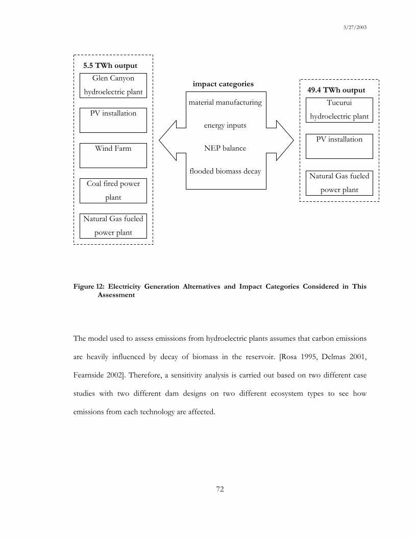
3/27/2003
72
Figure 12: Electricity Generation Alternatives and Impact Categories Considered in This Assessment
The model used to assess emissions from hydroelectric plants assumes that carbon emissions
are heavily influenced by decay of biomass in the reservoir. [Rosa 1995, Delmas 2001,
Fearnside 2002]. Therefore, a sensitivity analysis is carried out based on two different case
studies with two different dam designs on two different ecosystem types to see how
emissions from each technology are affected.
Tucurui
hydroelectric plant
49.4 TWh outputmaterial manufacturing
energy inputs
NEP balance
flooded biomass decay
PV installation
Natural Gas fueled
power plant
Glen Canyon
hydroelectric plant
Wind Farm
5.5 TWh output
PV installation
Natural Gas fueled
power plant
Coal fired power
plant
impact categories

3/27/2003
73
4.1.2.1 Glen Canyon Dam
Glen Canyon dam on the Colorado River is the second highest concrete arch dam in the U.S.
with 3,750,000 m3 of embedded concrete. Lake Powell, which is formed by water retained by
the 216 m high structure was completely flooded only in 1980 taking over 689 km2 of land
area [USBR 2001a]. The power plant, which began operation in 1964, is the second largest
operated by the U.S. Bureau of Reclamation (USBR) according to the electric output for all
facilities in 1999 [USBR 2001b].
Between 1984 and 1987, the generators were upgraded by 338 MW for a total of 1,296 MW.
The facility upgrade consisted of rewinding the generators and reducing the size of each
penstock (the tube transferring water into a turbine) from 15 to 14 inches in diameter [USBR
2001c]. The facility has 8 units; five generators are presently rated at 165 MW each, and three
generators are rated at 157 MW each. The upgrade of the existing dam has resulted in 39%
additional power [USBR 2001a]. Additional energy produced from the upgraded
hydroelectric power plant was 1.48 TWh in 1999. The contract cost to upgrade units 1, 3, 5,
and 6 was $7,044,724 ($26/kW), while it cost $5,026,724 ($30/kW) to upgrade units 2, 4, 7,
and 8, for a total upgrade cost of $12,071,448 in 1987 dollars [USBR 2001a]. The cost
calculations do not include the offset in upgrade cost by routine operation and maintenance
costs. Namely, normal maintenance costs would have been incurred to replace a worn
generator winding even if the upgrade had not occurred. This consideration makes upgrade
costs comparably smaller.
Based on detailed technical records [USBR 1970], GWP calculations, the GWE formula, and
the CO2 response function, the estimated GWE of Glen Canyon’s construction is 500,000

3/27/2003
74
MTCO2Eq (after 20 years) of operation. The contribution of construction materials and
processes, and power plant components is shown in Table 5. Emissions from excavation
were calculated based on the fuel consumption of the construction equipment, assuming
that all fuel was converted to CO2.
The GHG emissions from the upgrade were estimated assuming that all replaced parts came
from the sector that produces turbines and turbine generator sets. Since EIO-LCA in its
current version [EIO-LCA 2003] uses 1997 dollars, we converted the upgrade costs from
1987 to 1997 dollars using the Consumer Price Index (CPI) [BLS 2002]. The upgrade, which
increased power capacity by 39%, resulted in 10,000 metric tons of CO2 emissions, 1.3% of
the estimated CO2 emissions of Glen Canyon’s original construction (800,000 metric tons of
CO2).
While hydroelectric power plants do not use fossil fuels in operation, they emit GHGs from
biomass decay in the dam’s reservoir, a subject of debate lately [Rosa 1995, Gagnon 1997,
WCD 2000]. Annual biomass emissions are reduced as the flooded vegetation decays over
time. Colder climates have slower decay rates, thus lower annual emissions [Gagnon 1997].
For Glen Canyon, the assumptions were that (1) the area of the flooded land is similar to the
surface area of the reservoir, Lake Powell (653,130,000 m2), (2) originally the land was
covered by desert scrub that has a carbon density of 0.3 kg C/m2 [Harte 1988], (3) the e-
folding time for the biomass decay is 7 years, and (4) 10-30% of the carbon was subject to
anaerobic decomposition and released as CH4 [Rosa 1995]. Accordingly, using the CO2
response function, the GWE is estimated to be 2,000,000 – 5,000,000 MTCO2Eq (after 20
years).

3/27/2003
Table 5: Glen Canyon Hydroelectric Plant Construction Inputs and GWE (after 20 yr of operation) [Pacca 2002]
Unit cost Total cost GHG emissions (MT CO2 equiv.) Inputs: Total MT (1992 $/MT) (1992 $) CO2 + CH4 + N2O = GWE concrete 9,906,809 301 296,752,257 400,792 751 7,898 409,441excavation (m3) 4,711,405 n.a. 114,839,000 3,812 3,812turbines and turbine generator sets n.a. n.a. 65,193,084 41,725 45 249 42,019power distribution and transformers n.a. n.a. 13,754,764 12,358 16 79 12,453steel 32,183 3852 12,402,138 47,310 29 244 47,583Copper 90 2,3682 214,167 186 0 2 188aluminum 67 1,2682 84,804 157 0 2 159
total (rounded) 503,240,216 500,000 1,000 9,000 500,000
75
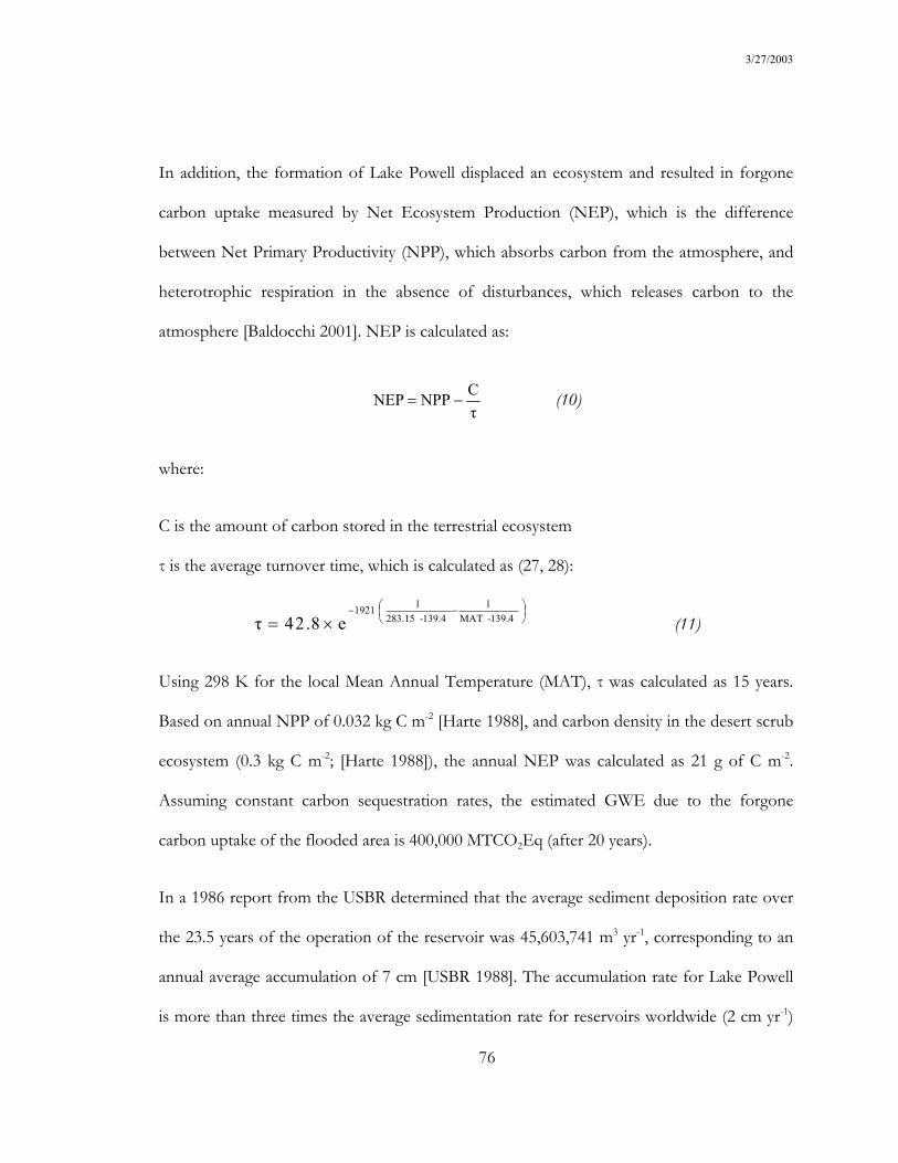
3/27/2003
76
In addition, the formation of Lake Powell displaced an ecosystem and resulted in forgone
carbon uptake measured by Net Ecosystem Production (NEP), which is the difference
between Net Primary Productivity (NPP), which absorbs carbon from the atmosphere, and
heterotrophic respiration in the absence of disturbances, which releases carbon to the
atmosphere [Baldocchi 2001]. NEP is calculated as:
τCNPPNEP −= (10)
where:
C is the amount of carbon stored in the terrestrial ecosystem
τ is the average turnover time, which is calculated as (27, 28):
−−
×= 139.4-MAT1
139.4-283.1511921
e8.24τ (11)
Using 298 K for the local Mean Annual Temperature (MAT), τ was calculated as 15 years.
Based on annual NPP of 0.032 kg C m-2 [Harte 1988], and carbon density in the desert scrub
ecosystem (0.3 kg C m-2; [Harte 1988]), the annual NEP was calculated as 21 g of C m-2.
Assuming constant carbon sequestration rates, the estimated GWE due to the forgone
carbon uptake of the flooded area is 400,000 MTCO2Eq (after 20 years).
In a 1986 report from the USBR determined that the average sediment deposition rate over
the 23.5 years of the operation of the reservoir was 45,603,741 m3 yr-1, corresponding to an
annual average accumulation of 7 cm [USBR 1988]. The accumulation rate for Lake Powell
is more than three times the average sedimentation rate for reservoirs worldwide (2 cm yr-1)
3/27/2003
77
[Mulholland 1982]. Assuming an average bulk density of 1 MT m-3 and 2% of organic carbon
[Dean 1998], the organic carbon accumulation rate equates to 912,075 MT per year, which
corresponds to 3,344,274 MTCO2Eq. This calculation assumes an average carbon percentage
in sediments; however, the climate of the Upper Colorado watershed is classified as semiarid,
and the lower part of the basin is sparsely vegetated because of inadequate rainfall and poor
soil conditions [USBR 1988]. Thus, the carbon content in the sediments is likely to be much
less. The burial of allochtonous carbon is not a sink for atmospheric carbon unless the
original source is being restored somewhere by means of photosynthesis [Stallard 1998].
Consequently, sedimentation is not considered as a carbon sink in this case.
Summing the two GHG emission sources (construction of the dam and biomass decay from
the reservoir) and the forgone NEP, the total GWE of the Glen Canyon Dam after 20 years
(at the time of the upgrade) is estimated at 3,000,000 – 6,000,000 MTCO2Eq.
Hydroelectric plants have been intensely criticized for changing and destroying the physical
environment, such as destroying natural habitat (e.g., of Pacific Northwest salmon) and
species, being unsightly (such as the flooding of Glen Canyon), siltation, dislodging
indigenous populations, etc. While undoubtedly important, these issues are not the subject
of this dissertation.
4.1.2.2 Tucurui Hydroelectric Plant
The importance of hydroelectricity in Brazil is demonstrated by the 93% (assuming 860 kcal
of oil equivalent per 1 kWh of electricity) share of this source in the country’s electricity
matrix, which corresponded to 322 TWh in the year 2000. The Ministry of Energy of Brazil
3/27/2003
78
estimates that the full exploitation of domestic hydroelectric resources could add 143 GW of
power to the existing 61 GW [BEN 2001].
When completed the Tucurui power plant on the Tocantins River will become the largest
hydroelectric plant entirely on Brazilian territory (The world’s largest power plant, Itaipu, is
on the border of Brazil and Paraguay). The power plant is located in the northern region, in
Pará state, at latitude 3° 45' S and longitude 49° 41' W. The Tocantins River is part of the
north-south Tocantins/Araguaia watershed, and flows into the Amazon River estuary. The
reservoir flooded 2,850 km2 of rain forest, and only 140 km2 of vegetation have been cleared
in advance [La Rovere 2000].
The reservoir, which is owned by the public utility Eletronorte (ELN) was filled in 1985-
1986, and the motorization of the power plant was divided in two phases. Phase I has been
already completed and is composed of twelve Francis-type turbines (369 MW each) and
generator sets plus two small auxiliary units (20 MW each). Phase II comprises of 11 Francis
turbines with 382 MW each. The expected total installed capacity of the power plant is 8,670
MW (Table 6). Assuming a capacity factor of 65% the power plant yields an annual energy
output of 49,367 TWh [ELN 2003].
The Tucurui dam is a concrete gravity dam with a total installed capacity of 8.67 GW. The
major structures are an earth dam on the right bank, a riprap dam on the river bed, and a
concrete spillway. Construction included 57,385,718 m3 of excavation, 84,682,890 m3 of
earthfill and rockfill, and 17,900,070 m3 of concrete. Initially, the cement was to be imported
from Colombia but the government decided to buy domestically produced cement at a
higher cost to support the local industry [La Rovere 2000]. Herein it is assumed that the

3/27/2003
79
cement comes from Recife, which is a major city in the northeast of Brazil, located 2,150 km
away from Belem [CDP 2003].
Table 6: Characteristics of the Turbine Generator Sets in Tucurui [La Rovere 2000]
Phase I Phase II
main auxiliary main
Number 12 2 11
Type Francis Francis Francis
Capacity 369 MW 20 MW 382 MW
Head 60.80 m 60.80m 61.7 m
Speed 81.80 rpm 327.27 rpm 81.80 rpm
Rotor Diameter 8.10 m n.a. 8.50 m
Flow Intake 575 m3/s 39.50 m3/s 679 m3/s
Generator Output 350 MVA 250 MVA 395 MVA
n.a. not available
The Tocantins River is navigable and 254 km separate the estuary, which is close to Belem,
the capital of Para State, from the dam. Tugboats are used for cargo transport in the
Tocantins/Araguaia system; thus, commodities are easily transported to Belem Port on the
Atlantic Ocean. This transportation mode was used to send materials and equipment used in
the construction of the power plant because of its lower cost compared to road
transportation. In fact, the improvement of the roads connecting Tucurui to the major cities
in the region was not accomplished during the construction phase as initially expected [La
Rovere 2000].

3/27/2003
80
Based on the characteristics of the reservoir and the GWE method [Pacca 2002], the
estimated GWE of Tucurui’s construction is 1,600,000 MTCO2Eq after 20 years (Table 7).
The contributions of construction materials and processes, transportation, and power plant
components are shown in Table 7. Emissions from excavation were calculated based on the
fuel consumption of the construction equipment, assuming that all fuel was converted to
CO2. Emissions from cement transportation were calculated assuming that 8% of the
concrete mass is cement that was shipped from Recife, combined with a fuel efficiency of
104 metric tons km-1 liter-1, and an emission factor of 2.8 kg of CO2 per liter of fuel oil
[Davis 2002, IPCC 1997].
While hydroelectric power plants do not use fossil fuels in operation, they emit GHGs from
biomass decay in the dam’s reservoir, a subject of debate lately [Rosa 1995, Gagnon 1997,
WCD 2000]. Yearly biomass emissions are reduced as the carbon previously stored in the
ecosystem decays over time. For Tucurui, the assumption was that the area of the flooded
land is similar to the surface area of the reservoir (2,430 km2) subtracting the old riverbed,
the islands and deforested areas, which yields a flooded area of 1,180 km2 [Rosa 2002].
Originally the land was covered by tropical forest that has a carbon density of 18.8 kg C m-2
[Harte 1988], the e-folding time (time required for an initial amount to decay to 1/e of its
initial mass) for the biomass decay is 7 years, and 10-30% of the carbon was subject to
anaerobic decomposition and released as CH4 [Rosa 1995]. Accordingly, assuming a
parameterized CO2 pulse response function, the GWE is estimated to be 118,576,083 to
355,728,188 MTCO2Eq (after 20 years of operation).
After 15 years, the contribution of biomass decay only equates to 42 to 126 MT km-2 yr-1 of
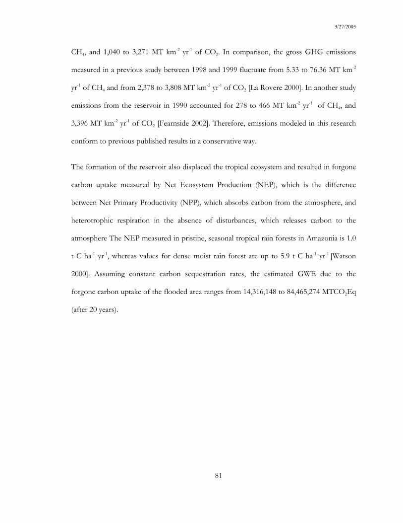
3/27/2003
81
CH4, and 1,040 to 3,271 MT km-2 yr-1 of CO2. In comparison, the gross GHG emissions
measured in a previous study between 1998 and 1999 fluctuate from 5.33 to 76.36 MT km-2
yr-1 of CH4 and from 2,378 to 3,808 MT km-2 yr-1 of CO2 [La Rovere 2000]. In another study
emissions from the reservoir in 1990 accounted for 278 to 466 MT km-2 yr-1 of CH4, and
3,396 MT km-2 yr-1 of CO2 [Fearnside 2002]. Therefore, emissions modeled in this research
conform to previous published results in a conservative way.
The formation of the reservoir also displaced the tropical ecosystem and resulted in forgone
carbon uptake measured by Net Ecosystem Production (NEP), which is the difference
between Net Primary Productivity (NPP), which absorbs carbon from the atmosphere, and
heterotrophic respiration in the absence of disturbances, which releases carbon to the
atmosphere The NEP measured in pristine, seasonal tropical rain forests in Amazonia is 1.0
t C ha-1 yr-1, whereas values for dense moist rain forest are up to 5.9 t C ha-1 yr-1 [Watson
2000]. Assuming constant carbon sequestration rates, the estimated GWE due to the
forgone carbon uptake of the flooded area ranges from 14,316,148 to 84,465,274 MTCO2Eq
(after 20 years).
3/27/2003
Table 7: Major Construction Inputs and GWE (after 20 yr of operation) for Tucurui Hydroelectric Planta
GHG emissions (MT of CO2 equiv) Inputs total MT
unit cost (1997 $/MT)
total cost (1997 $) CO2 + CH4 + N2O = GWE
concrete 17,900,070 $29.70 $531,590,919 380,412 390,130 697 771,239turbines and turbine generator sets n.a. n.a. $1,119,386,000 245,546 250,295 459 496,300Steel 203,440 $275.63 $56,074,916 60,853 52,782 66 113,702power distribution and transformers n.a. n.a. $99,245,000 31,435 30,336 55 61,825excavation (m3) 57,385,718 n.a. n.a. 54,570 54,570cement transportation (MT km-1) 3,805,916,004 n.a. n.a. 55,671 55,671earthfill and rockfill (m3) 84,682,890 n.a. n.a. 51,524 51,524
total 880,000 720,000 1,300 1,600,000a Total emissions are rounded to two significant digits. MT, metric ton; GWE, global warming effect; na, not available.
82
3/27/2003
83
If the productivity of the land ecosystem replaced is of concern, the productivity of the
aquatic environment may also affect the balance of carbon. High rates of sediment
deposition can bury organic sediments in anoxic strata slowing oxidation. Reservoirs can be
a carbon sink if the organic carbon that is being buried represents an increase in the input
into streams and rivers and if carbon in natural environments would have been oxidized
instead of buried in reservoirs. Indeed, a large fraction of the carbon fixed in freshwater
ecosystems is captured in the sediments because of shallower water columns, prevalence of
anoxic strata, higher NPP, and sedimentation rates. Large lakes have an accumulation rate of
2 to 10 g C m-2 yr-1 [Mulholland 1982]. Based on this numbers the Tucurui reservoir would
account for a carbon uptake of 286,323 to 143,615 MTCO2Eq (after 20 years).
Summing the two GHG emission sources (construction of the dam and biomass decay from
the reservoir) with the forgone NEP, and subtracting the carbon uptake by the reservoir, the
total GWE of the Tucurui Dam after 20 years (at the time of the upgrade) is estimated at
691,887,398 to 1,871,684,087 MTCO2Eq.
4.2 Photovoltaic Electricity Generation Systems
PV modules convert solar energy directly into electricity. Although several LCAs in the
literature show CO2 emissions normalized by electricity output of PV installations, different
assumptions used in each study make results difficult to compare; thus, the range of results
published is quite large. Table 8 shows a compilation of studies that published CO2
emissions associated with electricity generation using PV technology.

3/27/2003
84
Table 8: Published Carbon Dioxide Emissions per Kilowatt-hour for PV Systems.
Author year Characteristics gCO2/kWh
Fritsche 1989 n.a. 32.0
Meridien Corp. 1989 central station PV plant 6.5
San Martin 1989 central station PV plant 5.4
Kreith 1990 central PV system 100 MW 24.0
Uchiyama 1992 PV 201.3
Nieuwlaar 1996 roof integrated system - 30 m2 amorphous cells 47.0
Komiyama 1996 Japan – polycrystalline 522.0
Komiyama 1996 Indonesia – polycrystalline 1004.4
Dones 1998 PV p-Si (CH) - 100yr. GWP 189.0
Dones 1998 PV m-Si (CH) - 100yr. GWP 114.0
IEA 1998 mc-Si 87.0
Frankl 1998 monocrystalline silicon PV power plant 200.0
Kato 1998 single-crystalline silicon 83.0
Kato 1998 polycrystalline silicon (poly-Si) PV module - future
technology 20.0
Kato 1998 amorphous silicon (a-Si) PV module - future technology 17.0
Alsema 2000 thin film (amorphous) grid connected roof top systems
(1700 kWh m-2 yr-1) 30yr. lifetime 50.0
Alsema 2000 monocrystalline grid connected roof top systems (1700 kWh
m-2 yr-1) 30yr. lifetime 60.0
Greijer 2000
dye sensitized solar cell (ncDSC) 20 yrs. Lifetime - 2190
kWh m-2 yr-1 - 500MW plant - amorphous - Efficiency=7%
and process energy=100 kWh m-2
19.0
Greijer 2000 dye sensitized solar cell (ncDSC) 20 yrs. Lifetime - 2190
kWh m-2 yr-1 - 500MW plant - amorphous 47.0
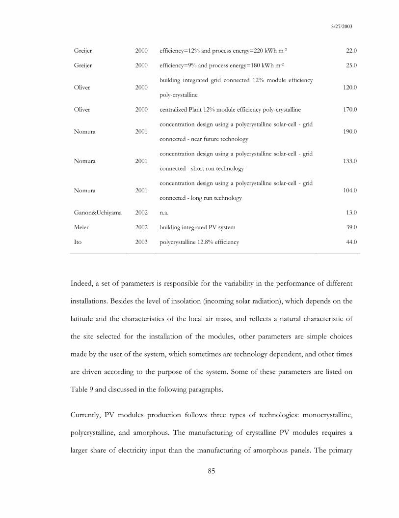
3/27/2003
85
Greijer 2000 efficiency=12% and process energy=220 kWh m-2 22.0
Greijer 2000 efficiency=9% and process energy=180 kWh m-2 25.0
Oliver 2000 building integrated grid connected 12% module efficiency
poly-crystalline 120.0
Oliver 2000 centralized Plant 12% module efficiency poly-crystalline 170.0
Nomura 2001 concentration design using a polycrystalline solar-cell - grid
connected - near future technology 190.0
Nomura 2001 concentration design using a polycrystalline solar-cell - grid
connected - short run technology 133.0
Nomura 2001 concentration design using a polycrystalline solar-cell - grid
connected - long run technology 104.0
Ganon&Uchiyama 2002 n.a. 13.0
Meier 2002 building integrated PV system 39.0
Ito 2003 polycrystalline 12.8% efficiency 44.0
Indeed, a set of parameters is responsible for the variability in the performance of different
installations. Besides the level of insolation (incoming solar radiation), which depends on the
latitude and the characteristics of the local air mass, and reflects a natural characteristic of
the site selected for the installation of the modules, other parameters are simple choices
made by the user of the system, which sometimes are technology dependent, and other times
are driven according to the purpose of the system. Some of these parameters are listed on
Table 9 and discussed in the following paragraphs.
Currently, PV modules production follows three types of technologies: monocrystalline,
polycrystalline, and amorphous. The manufacturing of crystalline PV modules requires a
larger share of electricity input than the manufacturing of amorphous panels. The primary
3/27/2003
86
energy required for the fabrication of crystalline PV modules is 3.8 to 2.9 times the input for
the same unit area of amorphous modules [Alsema 2000b]. Table 10 shows different phases
in the manufacturing of crystalline and amorphous modules and their respective energy
consumption. However, these estimations are contentious and the energy necessary for
manufacturing of crystalline modules varies between 2,400 and 7,600 MJ/m2 for
polycrystalline (mc-Si) technology and between 5,300 and 16,500 MJ/m2 for monocrystalline
(sc-Si) technology. Manufacturing energy requirement for thin film (amorphous) modules
ranges from 710 to 1,980 MJ m-2 [Alsema 2000b].
Table 9: Characteristic Parameters in a PV installation.
Technology System configuration
Module’s technology Array area
Module’s efficiency Tilt angle and/or orientation
Tracking system Mounting structure
Components’ lifetime Stand alone vs. grid connected
Installation scale
Other B.O.S. components
Although the energy required for manufacturing PV modules is more a function of the
modules’ area than its power [Alsema 2000], other studies report the manufacturing energy
normalized to the power output. For example, the manufacturing of a 11.2% efficient

3/27/2003
87
monocrystalline module requires 9,683 kWh/kWp of electricity, whereas the manufacturing
of a 10.3% efficiency polycrystalline module requires 12,723 kWh/kWp [Frankl 1998].
Assuming Standard Test Conditions (irradiance level of 1,000 W m-2), these values equate to
3,904 MJ m-2 and 4,718 MJ m-2 respectively, which allows the comparison with the ones
presented in Table 10.
The primary energy input in the manufacturing phase affects the energy pay back ratio of the
modules, depending on which is the source of the energy mix used, the embedded emissions
are remarkable. Most GHGs emissions associated with PV systems (80 to 90%) are linked to
electricity requirements in the fabrication of modules. The energy mix that goes into the
manufacturing of the module is crucial to its GHG emissions. Thus, the substitution of
renewable electricity for fossil based electricity in the manufacturing of the modules would
reduce its emissions [Dones 1998]. In addition, the energy consumed to produce the
machinery used to make PV modules is not negligible (Alsema 2000].
Table 10: Energy Requirements for Module Manufacturing (MJ/m2) (Adapted from
[Alsema 2000])
Process Crystalline Amorphous
Silicon mining and purification 2,200 Cell
material Silicon wafer production 1,000*
50
Cell module processing 300 400
Module encapsulation materials 200 350

3/27/2003
88
Overhead operation and equipment manufacturing 500 400
Total module (without frame) 4,200 1,200
Module frame (aluminum) 400 400
Total module (framed) 4,600 1,600
*monocrystalline wafers require an additional 1,500 MJ m-2
Of course, the energy conversion efficiency of the modules also affects the energy pay back
ratio of PV systems. The energy conversion efficiency measures the ratio between the
electric output of the panel and the incoming solar radiation on the surface of the module,
and is expressed as a percentage. The efficiency of a module is a function of the technology
used; therefore, different brands, vintages, and types of modules will have different
efficiencies. Improving both the energy conversion efficiency of the modules and their
manufacturing efficiency, that is, reducing energy and materials inputs, affects the cost of the
electricity produced out of PV installations. The continuous growth of the PV industry has
benefited from both practices that ultimately reflect in the penetration of the technology in
the market and affects the electricity cost. Such evolution in the industry is usually captured
by a learning curve with the plot of the logarithm of the average electricity cost versus the
cumulative sales of modules (Figure 13).

3/27/2003
89
Experience curve for PV modules on the world market. The price for a module is given in constant 1992 US$ per peak watt,Wp. Peak watts are the power output from the module at optimum solar conditions as defined by certification agencies. Adopted from Williams
and Terzian (1993).
Figure 13: Learning Curve for PV Modules [IEA 2000b]
The quality of the crystallization process is key to the final efficiency of the module.
Depending on the technology, the efficiency of the modules also decreases with use.
Technological changes are constantly improving the efficiency of the modules and reducing
their costs. Monocrystalline ingots, which are harder to obtain, are used in the manufacturing
of modules with the highest efficiencies whereas polycrystalline materials are cheaper and
produce modules with efficiencies 1 to 2 % lower than monocrystalline modules. Between
the production of electronic grade silicon and the wafers, 60% of the silicon is lost due to
quality concerns [Alsema 2000]. Because the production of crystallized silicon demands a
significant amount of energy, silicon losses affect negatively the energy payback ratio of the
modules and their life-cycle emissions.
3/27/2003
90
Because the electricity output of a module depends on how much solar radiation reaches the
surface of the module, the position of the module with respect to the sun is important. The
electricity produced by the module depends on the direction of the module’s face and the
angle with the horizontal plane. Some module’s arrays are equipped with a frame that tracks
the sun and increases the amount of incoming radiation. While some of the arrays move only
along one axis based on a frame filled with refrigerating gas, other tracking systems move
along four axes and are powered by a small electric motor. In this case some electricity
generated by the system is consumed during its operation [Keoleian 1997].
The choice of the tilt angle depends not only on the maximization of the energy output of
the modules, which varies with the seasons of the year, but also on the economic and
environmental cost of the structures to hold the modules. The feasibility of such systems
also depends on the balance between economic and environmental costs and benefits.
The Balance of the System (BOS) is the term used to refer to all the other components in
the PV installation in addition to the modules. The BOS depends on the type of application
and local conditions, and includes the structure to support the modules and hardware.
Batteries to store and deliver energy during load periods, as well as inverters might be
necessary if the system is connected to the grid that operates with alternate current. Cables
to interconnect modules and arrays to batteries and inverters are also part of the BOS.
Batteries have emission impacts throughout their life-cycle. The assessment of the energy,
and carbon and other emissions associated with the BOS should also be part of a
comprehensive LCA. The table below shows energy use estimations for components used in
the BOS.

3/27/2003
91
Table 11: Energy Inputs into System Components: [Alsema 2000b]
Aluminum module frame MJ/m2 500
Array support – central plant MJ/m2 1800
Array support – rooftop MJ/m2 700
inverter (3 kW) MJ/W 1
Whenever energy is converted or stored to be further recovered, some losses occur;
therefore, there are some efficiency losses associated with these practices that need to be
included in the analysis. It is estimated that 25% of energy is lost in the system through BOS
conversion efficiency losses [Alsema 2000].
A basic difference between systems is with respect to the purpose of the installation. While
some PV systems are stand-alone systems that can only supply energy for small consumers,
others are grid-connected. The scale of grid-connected systems is variable and this parameter
affects the BOS of the system and its respective material requirements. Figure 14 shows a
comparison of energy and material inputs in six different configuration for grid connected
systems using monocrystalline (m-Si) and policrystalline PV modules (p-Si) [Dones 1998].
The assumed efficiency for the m-Si and p-Si modules is 16.5% and 14% respectively. Roof
modules produce 860 kWh per year per kWp whereas the 100 kW plant produces 1000 kWh
per year per kWp and the 500 kW plant produces 1200 kWh per year per kWp.
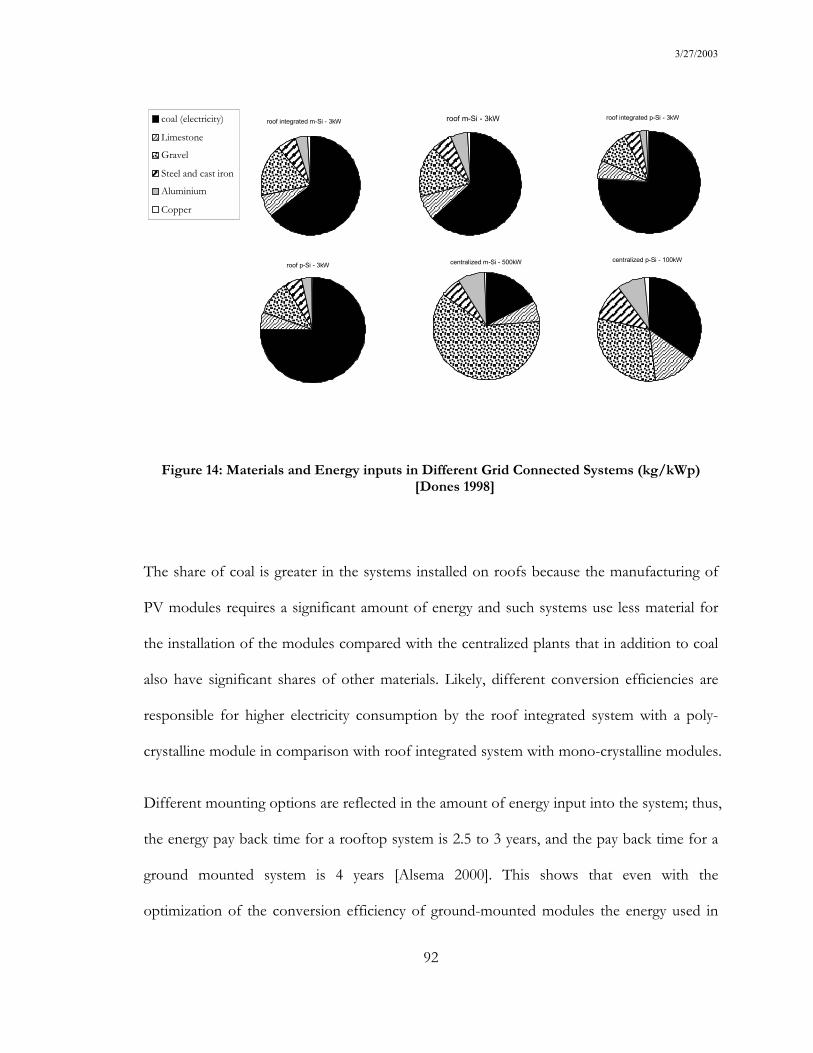
3/27/2003
92
roof integrated m-Si - 3kWcoal (electricity) Limestone Gravel Steel and cast iron Aluminium Copper
roof m-Si - 3kW roof integrated p-Si - 3kW
roof p-Si - 3kW centralized m-Si - 500kW centralized p-Si - 100kW
Figure 14: Materials and Energy inputs in Different Grid Connected Systems (kg/kWp) [Dones 1998]
The share of coal is greater in the systems installed on roofs because the manufacturing of
PV modules requires a significant amount of energy and such systems use less material for
the installation of the modules compared with the centralized plants that in addition to coal
also have significant shares of other materials. Likely, different conversion efficiencies are
responsible for higher electricity consumption by the roof integrated system with a poly-
crystalline module in comparison with roof integrated system with mono-crystalline modules.
Different mounting options are reflected in the amount of energy input into the system; thus,
the energy pay back time for a rooftop system is 2.5 to 3 years, and the pay back time for a
ground mounted system is 4 years [Alsema 2000]. This shows that even with the
optimization of the conversion efficiency of ground-mounted modules the energy used in

3/27/2003
93
the structures to support the modules drains a considerable amount of energy. Indeed,
concrete and steel used in the construction of the structures to support the modules are
responsible for the high energy content of the PV plants [Frankl 1998]. The use of an
existing structure to support the modules also reduces the footprint of this electricity
generation alternative since the structure stands in that place for other reasons than just to
support the modules.
In urbanized settings grid connected modules are placed on existing building structures.
Such installation is known as building-integrated PV (BIPV) [Keoleian 2003]. While rooftop
modules are placed on an existing structure through the use of simple frames to hold a set of
modules, stand-alone systems demand the manufacturing and installation of special frames
on the ground to hold an array, which includes a set of modules.
Although small producers may own grid-connected systems, the aggregation of several small
suppliers in a network may result in a significant energy source, which could be comparable
to centralized power plants. Actually, when a large number of individual modules are
connected to the grid the scale of the system can be compared with the capacity of a PV
power plant where all modules are located side by side in the same place. Advantages of a
network system include its resilience to massive power outages that are characteristic in
large-scale centralized systems, and the elimination of power transmission losses when
modules are installed close to consumers. [Pearce 2002]. In a recent study distribution losses
where calculated as 7.03% of the power delivered to the grid [Spath 1999].
The scale of grid-connected systems varies, and although a collection of small modules may
match the energy produced in a larger installation there are some advantages due to
3/27/2003
94
economies of scale in the construction of large-scale centralized systems. One advantage of a
centralized system is that the materials used in the facility can be reused, recovered, and
recycled more easily than if they were in dispersed installations [Fthenakis 2000]. Changing
the position of the panels to maximize the amount of incoming radiation in their surfaces
may also be easier in a centralized plant. In Japan large-scale centralized plants (100 MW) are
expected to be constructed over the next couple of years [Pearce 2002].
A comparison between crystalline and amorphous technologies shows that more efficient
crystalline modules consume more energy during manufacturing than less efficient
amorphous modules. However, the efficiency of amorphous modules diminishes over time
whereas the efficiency of crystalline modules lasts longer. Therefore the decreasing efficiency
of amorphous modules over time needs to be factored into the analysis. The efficiency of
amorphous modules typically declines about 25% over the first few months of exposure to
the sun due to the Staebler-Wronski effect [Staebler 1977], but then the efficiency stabilizes
and the quality of the modules do not continue to degrade after this point for the life-cycle
of the PV.
In a LCA all emissions, including emissions during manufacturing, are compared to the
energy produced over a certain period. Usually this period is the lifetime of a major
component of the system. In the case of PV systems 25 to 30 years is used as the lifetime of
the modules. However, for some types of amorphous modules a lifetime between 10 to 20
years is more realistic even if some higher performance brands such as the triple junction
Unisolar modules may reach 25 to 30 years of life time [Jacobson 2003]. While some
parameters are choices made by the investor others are circumstantial, that is, they depend
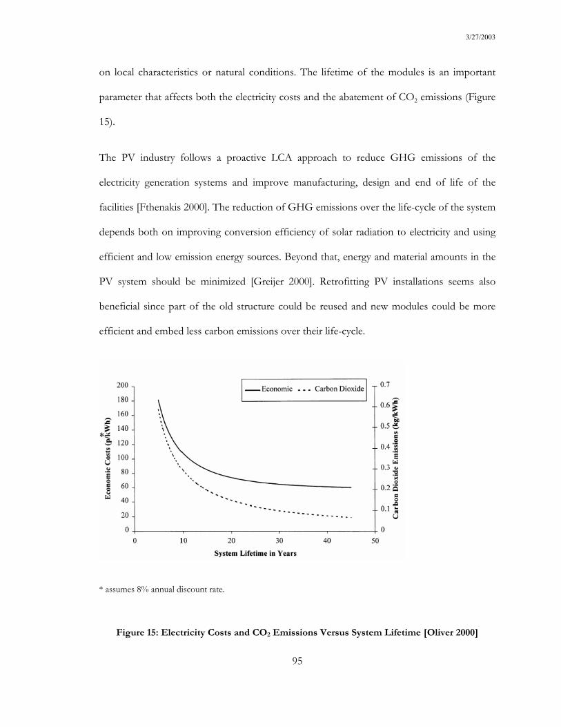
3/27/2003
95
on local characteristics or natural conditions. The lifetime of the modules is an important
parameter that affects both the electricity costs and the abatement of CO2 emissions (Figure
15).
The PV industry follows a proactive LCA approach to reduce GHG emissions of the
electricity generation systems and improve manufacturing, design and end of life of the
facilities [Fthenakis 2000]. The reduction of GHG emissions over the life-cycle of the system
depends both on improving conversion efficiency of solar radiation to electricity and using
efficient and low emission energy sources. Beyond that, energy and material amounts in the
PV system should be minimized [Greijer 2000]. Retrofitting PV installations seems also
beneficial since part of the old structure could be reused and new modules could be more
efficient and embed less carbon emissions over their life-cycle.
* assumes 8% annual discount rate.
Figure 15: Electricity Costs and CO2 Emissions Versus System Lifetime [Oliver 2000]
*
3/27/2003
96
4.2.1 Global Warming Effect of a PV System
In this section the GWE method is applied to two case studies that consider the installation
of massive and centralized PV plants as a replacement of large hydroelectric plants. The first
one in the desert takes into account the replacement of the energy generated at Glen Canyon
hydroelectric plant and the second one in a tropical forest assumes the replacement of
energy generated at the Tucurui hydroelectric plant.
4.2.1.1 PV System in a Dry Ecosystem
Medium-sized PV plants of 1 MW capacity are considered the functional unit [Tahara 1997].
Ordinarily, large capacity solar plants are designed as thermal systems instead of
incorporating PVs. These plants use reflective surfaces to focus sunlight on a collector that
contains a working fluid (e.g., an oil-filled tube). The heat from the working fluid is
transferred to water, and the resulting steam powers a turbine-generator set to produce
electricity [Johanson 1993]. This setup would be more appropriate at the scale under
consideration here; however, solar industry trends point toward PV module production.
Manufacturing and constructing a PV plant to match the annual electricity output of Glen
Canyon power plant (5.55 TWh) would result in a GWE of 10,000,000 MTCO2Eq after 20
years of operation (Table 12). The total cost of materials and construction was
$3,578,458,000 (in 1997 dollars), excluding land purchases, labor/installation and
maintenance costs.
About 35 million 100 W modules of dimensions 1.316x0.66 m2 [Shellsolar 2003] could be
3/27/2003
97
used in a non-concentrating array composed of array units of 3x10 panels, each having its
own concrete foundation, for a surface area of 3.9x6.6 m2, sited at 30 degrees latitude, at a
30-degree tilt (approximately 1.2 m of additional width is needed to account for shading by
the array due to the sun’s angle). There is 0.9 m between each of these array units for
personnel access. Each adjacent unit covers a land area of 37.44 m2, and has a capacity rating
of 3 kW. Some 1,372,52400 of these 3 kW units are required [NREL 1991]. The upgraded
Glen Canyon plant yields 5.55 TWh of energy each year from a capacity of 1,296 MW. Since
the PV plant will have a smaller capacity factor (due to solar resource availability), the
necessary installed capacity to achieve the same delivered energy is 4,118 MW, more than
three times the hydroelectric plant’s capacity. By comparison, the world production of PV
modules was 260 MW in 2000 [Pearce 2002], thus meeting the capacity with PV is
unreachable without major investments in production capacity or new technological
breakthroughs.
The PV array required in this analysis would demand approximately 51,386,400 m2 of land
area. Land costs will vary depending on location. A PV plant of this magnitude must be
constructed in a remote area such as a desert where land prices are low and solar resource is
high. Given a range of prices between $250 and $1,200 per ha, the required land would add
an additional $1,269,234000 to $6,346,171000 to the cost of the PV plant, an insignificant
amount given the total life-cycle cost of $3.6 billion. The cost of land is reduced when the
PV system is distributed, i.e., the generating capacity required is spread over a larger number
of small systems (e.g., existing rooftops).
It was assumed that after 30 years of operation [Stronberg 1998] all PV panels had to be
3/27/2003
98
replaced (but not the concrete and steel base), and that the required construction energy was
100% of the original due to an energy-intensive PV manufacturing process. The electricity
output of the facility remained constant. The refurbishment resulted in 4,000,000 metric tons
of CO2 emissions, a quarter of the original emissions from manufacturing and construction
(20,000,000 metric tons of CO2).
The solar plant would displace an ecosystem similar to what Glen Canyon Dam’s reservoir
flooded. The NEP loss is estimated at 30,000 MTCO2Eq, and the decay of the biomass
removed from the site during construction amounts to 40,000 MTCO2Eq (assuming the
same ecosystem conditions as for the Glen Canyon site, measured after 20 years). Therefore,
the total GWE of the PV plant (accounting for the manufacturing, construction, and NEP
loss) would amount to 10,000,000 MTCO2Eq 20 years after construction.

3/27/2003
99
Table 12: Major Construction Inputs and GWE (after 20 yr) for a PV Plant
GHG emissions (MT CO2 equiv.) Inputs: Total MT
Unit cost (1992 $/MT)
Total cost (1992 $) CO2 + CH4 + N2O = GWE
steel 4,600,276 3851 1,772,797,382 6,957,724 4,216 35,924 6,997,865
copper 480,029 2,3681 1,136,805,659 984,580 1,617 10,504 996,701
electricity (MWh) 7,556,010 362 268,780,863 2,152,447 1,077 20,407 2,173,931
aluminum 177,788 1,2681 225,374,699 428,610 405 6,558 435,573
cement 2,222,356 551 121,362,849 410,263 394 15,497 426,153
glass 1,066,731 501 53,336,538 56,951 67 759 57,777
total (rounded) 3,578,457,990 10,000,000 8,000 90,000 10,000,000
1USGS 2002
2 IEA 2000

3/27/2003
100
4.2.1.2 PV System in a Tropical Forest
Because the solar industry is currently based on the production of PV modules, which
convert solar energy directly into electricity, medium-sized PV plants of 1 MW capacity are
considered the functional unit in this analysis [Tahara 1997]. Manufacturing and constructing
a PV plant for the required annual electricity output of Tucurui (49,367 GWh) would result
in a GWE of 30,000,000 MTCO2Eq after 20 years of operation (Table 13).
The installation would use 110 W (1.32 x 0.66 m) monocrystalline modules with a rated
efficiency of 12.66% [Shell 2003]. They would be mounted in a non-concentrating array
consisting of 3 x 10 panels positioned at an angle corresponding to the local latitude to
maximize the average daily output. Each array is anchored in a 2 m3 concrete foundation,
and covers a 37.8 m2 area. The arrays are arranged on sets that are serviced by 2 m wide
asphalt paved roads. Each unit has 2 rows of 10 arrays with 1.2 m between the 2 rows to
account for shading by the array due to the sun’s angle, and 0.9 m between each of these
array units for personnel access.
Some 8,541,603 of these 3.3 kW units are required to meet the output of Tucurui, based on
the available insolation [Sundata 2003]. Since the PV plant will have a smaller capacity factor
(due to solar resource availability) than Tucurui, the necessary installed capacity to achieve
the same delivered energy is 25,600 MW, three times the hydroelectric plant’s capacity. By
comparison, the world production of PV modules in 2000 was 260 MW [Pearce 2002]. Thus
meeting the capacity with PV is unreachable without major investments in production
capacity or new technological breakthroughs.
3/27/2003
101
Because there is no PV manufacturer in Brazil it was assumed that the modules would be
shipped from Europe. Each module weighs 11 kg and the distance between the supplier and
the construction site is 6,760 km, which includes a round trip between the Port of Belem and
Tucurui besides the distance between the two continents. Marine transportation is used for
the modules’ shipment.
The PV array required in this analysis would demand approximately 331 km2 of land area,
which corresponds to 12% of the reservoir’s area. It was assumed that after 30 years of
operation [Stronberg 1998] all PV panels had to be replaced (but not the concrete
foundation and the steel support), and that the required construction energy at that time was
100% of the original due to an energy-intensive PV manufacturing process. The electricity
output of the facility remained constant. The refurbishment resulted in emissions of
12,000,000 MTCO2Eq, over a third of the original emissions from manufacturing and
construction (30,000,000 metric tons of CO2).
Similarly to Tucurui, the solar plant would displace a tropical forest. After 20 years, the NEP
loss is estimated at 1,662,081 to 9,806,280 MTCO2Eq, and the decay of the biomass
removed from the site during construction amounts to 12,400,000 MTCO2Eq (assuming
that all carbon is emitted as CO2). Therefore, the total GWE of the PV plant (accounting for
the manufacturing, construction, and NEP loss) would amount to 47,060,000 MTCO2Eq 20
years after construction. A sensitivity analysis was carried out assuming that a different
module technology is used in the installation. If amorphous modules with a 8.49% efficiency
replace the monocrystalline modules, the land required would amount to 582 km2 and
emissions reach 129,699,433 MTCO2Eq 20 years after construction.
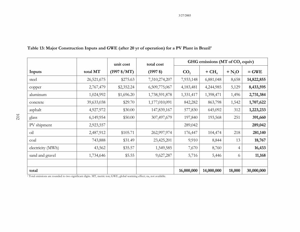
3/27/2003
Table 13: Major Construction Inputs and GWE (after 20 yr of operation) for a PV Plant in Brazila
GHG emissions (MT of CO2 equiv)
Inputs total MT unit cost
(1997 $/MT)total cost (1997 $) CO2 + CH4 + N2O = GWE
steel 26,521,675 $275.63 7,310,274,207 7,933,148 6,881,048 8,658 14,822,855copper 2,767,479 $2,352.24 6,509,775,067 4,183,481 4,244,985 5,129 8,433,595aluminum 1,024,992 $1,696.20 1,738,591,878 1,331,417 1,398,471 1,496 2,731,384concrete 39,633,038 $29.70 1,177,010,091 842,282 863,798 1,542 1,707,622asphalt 4,927,972 $30.00 147,839,167 577,830 645,092 312 1,223,233glass 6,149,954 $50.00 307,497,679 197,840 193,568 251 391,660PV shipment 2,923,557 289,042 289,042oil 2,487,912 $105.71 262,997,974 176,447 104,474 218 281,140coal 743,888 $31.49 23,425,201 9,910 8,844 13 18,767electricity (MWh) 43,562 $35.57 1,549,585 7,670 8,760 4 16,433sand and gravel 1,734,646 $5.55 9,627,287 5,716 5,446 6 11,168
total 16,000,000 14,000,000 18,000 30,000,000a Total emissions are rounded to two significant digits. MT, metric ton; GWE, global warming effect; na, not available.
102

3/27/2003
103
4.3 Wind
The installation of new wind turbines in Europe is ramping up; in the year 2002 over 23 MW
of new capacity have been added, which corresponds to a 33% increase [Johnson 2003]. In
the U.S. the numbers are still modest but thanks to dropping costs, more reliable systems,
tax credits, and regulatory requirements demanding a share of renewable energy in the
utilities electricity mix, EIA expects a 300% increase in the installed capacity over the next 25
years. Sizes and shapes of new projects in the U.S. span from a couple of turbines in a
school in Iowa to hundreds of MWs in a Californian desert or at off shore installation in the
northeastern region.
Although the technology of most modern wind turbines is equivalent, results from LCAs of
their energy and CO2 emissions vary [Lenzen 2002]. One basic difference is the location of
wind turbines, which can be on land or offshore. Recently, the installation of offshore
turbines, such as the proposed 170 MW project on Cape Cod, has attracted the attention of
investors [Angelo 2002]. The foundation requirements for offshore wind turbines are
different from the requirements for land based turbines. The energy intensity of turbine’s
tower is associated with the materials used in its construction. A concrete tower requires half
the energy of a steel tower [Lenzen 2002]. Offshore support structures require more material
and are more energy intensive to install.
A recent literature review shows that CO2 emission factors for wind power plants range is
7.9-123.7 g of CO2/kWh, capacity factors are 7.6-50.4%, and lifetime of the facilities is 15-30
years [Lenzen 2002]. Table 14 presents results from various emission assessment studies,

3/27/2003
104
which indicates that the reported values are between 7 and 74 g of CO2/kWh.
Table 14: Published Carbon Dioxide Emissions per Kilowatt-hour for Wind Farms
Author year Characteristics gCO2/kWh
Fritsche 1989 15
San Martin 1989 wind energy conversion system 7
Uchiyama 1992 Wind 100 kW turbine 74
Kuemmel 1997 Danish average system 16
Dones 1998 wind mix (CH) - 100yr. GWP 36
IEA 1998 8
Schleisner 2000 Offshore 5 MW – 500 kW turbine 17
Schleisner 2000 Land based 9 MW – 500 kW turbine 10
Voorspools 2000 coast 9
Voorspools 2000 Inland 25
Nomura&Inaba 2001 100 kW turbine 38
Ganon&Uchiyama 2002 9
Combining the GWE with a list of inputs provided by recent LCAs of wind farms minimizes
problems arising from the use of different assumptions related to the impacts of basic inputs
in the power plant life-cycle. However, such information is not readily available in the
literature, and moreover, it is inconsistent. The technology of wind turbines is changing
rapidly. In the beginning the most efficient turbines were in the 50 to 200 kW range but
currently they are in the 1 to 3 MW range. Both their weight and cost per installed capacity is
lower than the previous technology [Johnson 2003]. Table 15 presents a list of material
inputs to wind farms based on different turbine sizes.
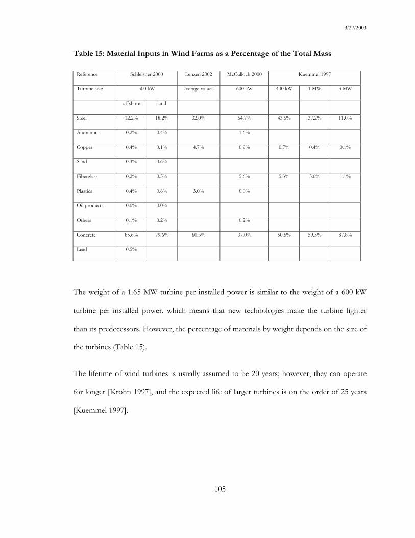
3/27/2003
105
Table 15: Material Inputs in Wind Farms as a Percentage of the Total Mass
Reference Schleisner 2000 Lenzen 2002 McCulloch 2000 Kuemmel 1997
Turbine size 500 kW average values 600 kW 400 kW 1 MW 3 MW
offshore land
Steel 12.2% 18.2% 32.0% 54.7% 43.5% 37.2% 11.0%
Aluminum 0.2% 0.4% 1.6%
Copper 0.4% 0.1% 4.7% 0.9% 0.7% 0.4% 0.1%
Sand 0.3% 0.6%
Fiberglass 0.2% 0.3% 5.6% 5.3% 3.0% 1.1%
Plastics 0.4% 0.6% 3.0% 0.0%
Oil products 0.0% 0.0%
Others 0.1% 0.2% 0.2%
Concrete 85.6% 79.6% 60.3% 37.0% 50.5% 59.5% 87.8%
Lead 0.5%
The weight of a 1.65 MW turbine per installed power is similar to the weight of a 600 kW
turbine per installed power, which means that new technologies make the turbine lighter
than its predecessors. However, the percentage of materials by weight depends on the size of
the turbines (Table 15).
The lifetime of wind turbines is usually assumed to be 20 years; however, they can operate
for longer [Krohn 1997], and the expected life of larger turbines is on the order of 25 years
[Kuemmel 1997].
3/27/2003
106
4.3.1 Global Warming Effect of a Wind Farm in the U.S.
In this assessment the feasibility of a wind farm is investigated as replacement for the energy
generated by Glen Canyon hydroelectric plant. A wind farm producing 5.55 TWh of
electricity per year was assumed to be in southern Utah, the same geographic area as Glen
Canyon, at an elevation of 2,134 m (7,000 ft), close to the Escalante Desert where the
average wind speed is 6.5 m/s [PNNL 1986]. A turbine of 600 kW [Schleisner 2000] was
used as the unit for the farm’s total of 4,480 turbines that would occupy an area of
48,9580,000 m2. The total cost of materials and construction of the facility would amount to
$206,881,000 (in 1992 dollars) without labor/installation and maintenance costs. Given a
range of prices between $250 and $1,200 per ha, the required land would add an additional
$12,098,162000 to $60,490,811000 to the cost. Given the large area, land between the
turbines could be used for other activities such as agriculture. No NEP loss was anticipated.
It was assumed that after 20 years of operation all turbines had to be replaced (but not the
concrete foundations), and that the required construction energy was 30% of the original
electricity and 100% of the petroleum used. The electricity output of the facility remained
constant. The refurbishment resulted in 900,000 metric tons of CO2 emissions, two-thirds of
the original emissions from manufacturing and constructing the plant (1,300,000 metric tons
of CO2). The contribution of construction materials and energy to the GWE of the wind
farm after 20 years of operation (800,000 MTCO2Eq) is shown in Table 16. Therefore, the
total GWE of the wind farm (accounting for the manufacturing, construction, and
refurbishment) would amount to 2,000,000 MTCO2Eq 20 years after construction.

3/27/2003
Table 16: Major Construction Inputs and GWE (after 20 yr of operation) for a Wind Farm in the U.S.
GHG emissions (MT CO2 equiv.) Inputs: Total MT
Unit cost (1992 $/MT)
Total cost (1992 $) CO2 + CH4 + N2O = GWE
steel 289,987 3851 111,751,615 426,296 258 2201 428,755electricity (MWh)* 1,691,678 362 40,756,138 317,231 158 3008 320,397concrete 1,266,172 303 37,927,398 51,225 96 1009 52,330aluminum 6,275 1,2681 7,954,337 14,703 13 225 14,941plastics 20,169 2204 4,445,273 5,090 7 53 5,150copper 1,569 2,3681 3,715,021 3,127 4 33 3,164glass 4,930 501 246,511 256 0 3 259oil 448 1062 47,380 204 0 1 205sand 9,412 41 37,743 55 0 0 55total (rounded) 206,881,416 800,000 500 7,000 800,000107

3/27/2003
108
4.4 Coal
Approximately 56% of all utility-produced electricity in the U.S. is generated by coal-fired
power plants. Electricity production from coal typically involves a sequence of phases
(Figure 16). However, the majority of the environmental impacts are associated with the
operation of the power plant and the disposal of by-products generated during combustion.
Figure 16: Coal Power Generation Life-cycle Phases
Results from published LCAs show that over 93% of the GHGs emissions from electricity
generated by coal power plants are released during fuel combustion (Table 17). Indeed, the
extraction of the chemical energy from coal, which in the U.S. averages 21.072 million Btu
per short ton [U.S. EIA 2003], is directly proportional to the amount of fuel combusted.
Table 17 also shows that recent LCAs report very small emissions associated with coal
power plants; however, the technology considered in these schemes that usually involves a
coal gasification phase has not been demonstrated yet. Actually, only three integrated
gasification combined cycle (IGCC) power plants completed in the U.S. have their
performance scrutinized by the National Energy Technology Laboratory (NETL) indicating
that the maximum CO2 emissions attained is 20% less than conventional technology [NETL
2003].
Coal Preparation
Installation and Construction
Maintenance End-of-life Operation Coal Mining Waste Disposal

3/27/2003
109
Conventional coal-fired power plants consist of a boiler that produces steam that is injected
in a turbine that is coupled to an electric generator. More advanced designs, such as IGCC
plants are based on the gasification of coal and the utilization of a combined cycle scheme to
maximize the conversion efficiency of the power plant. A combined cycle scheme involves
the use of two turbines in series and the reuse of the heat in the exhaust of the first turbine
to power the second turbine. Nowadays, it is possible to reach 60% energy conversion
efficiency through IGCC technology [Lombardi 2003]. Alternatively, the fuel obtained from
coal gasification could be used in a fuel cell that also attains high efficiencies.
Table 17: Published Carbon Dioxide Emissions per Kilowatt-hour for Coal-fired
Power Plants.
Author Year Characteristics Capacity
(MW)
combustion
share g/kWh
Fritsche 1989 929
Meridien Corp. 1989 Conventional coal plant with a scrubber 500 99.90% 1166
Meridien Corp. 1989 Atmospheric fluidized bed combustion plant (AFBC) 500 99.90% 1163
Meridien Corp. 1989 Integrated gasification combined cycle plant (IGCC) 1,000 908
San Martin 1989 Integrated gasification combined cycle plant (IGCC) 751
San Martin 1989 Conventional pulverized coal plant 500 99.79% 964
San Martin 1989 Atmospheric fluidized bed combustion plant (AFBC) 500 99.79% 962
Kreith 1990 Fluidized bed combustion 747 1041
Uchiyama 1992 Coal 1000 989
ORNL 1994 Pulverized Fuel - Southeast 500 99.91% 1230
ORNL 1994 Pulverized Fuel - Southwest 500 99.91% 1279
Nieuwlaar 1996 Integrated Coal Gasification Combined Cycle 600 800
Audus 1997 Steam cycle - no carbon capture - 43% efficient 775
Audus 1997 IGCC - 32% efficiency 135

3/27/2003
110
Tahara 1997 Commercially available 75% CF 39% efficiency 1000 915
Dones - GaBE 1998 Lignite - 100yr. GWP 1340
Dones - GaBE 1998 Hard coal PC - 100yr. GWP 1071
IEA 1998 Hard coal 1000
Spath 1999 Average System - 60% CF – 32% efficiency 360 93.30% 1022
Spath 1999 New Source Performance Standards (NSPS) 60% CF– 35% efficiency 425 92.70% 941
Spath 1999 Low Emission Boiler System (LEBS) 60% CF– 42% efficiency 404 95.60% 741
Nomura 2001 IGCC - oxygen-blowing - 70% CF 6000 810
Ganon&Uchiyama 2002 Existing plant without SO2 scrubbing 1050
Ganon&Uchiyama 2002 Modern plant with SO2 scrubbing 960
Lombardi 2003 Semi closed gas turbine combined cycle (SCGT/CC) 46 % efficiency 243 65
Lombardi 2003 (IGCC/CC) 39% efficiency 288 130
Molten-carbonate fuel cells (MCFC) reach high electricity generating efficiencies. When the
fuel cell is coupled to a turbine in a combined cycle scheme the 65% efficiency is superior to
IGCC [Srinivasan 1999]. The operation of MCFC involves a cathodic reaction that
consumes oxygen and CO2 and produces carbonate ions. These ions are transferred through
an electrolyte to the anode where hydrogen reacts with carbonate to produce water and CO2,
which is fed back into the cathodic reaction.
In the case of more traditional technology, the boiler is a central device in any thermal power
plant. The boiler is where the heat produced from the fuel combustion is transferred to a
fluid that is further used to run the turbine. The technology used in boilers is continuously
evolving. Flue bed and pulverized fuel (PF) boilers are the most common designs, which
also refer to the lay-out of the combustion chambers. In the future, pulverized coal boilers
known as new source performance standards (NSPS) with 35% conversion efficiency and
low emission boiler systems (LEBS) with 42% conversion efficiency are expected to produce
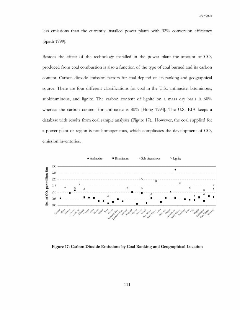
3/27/2003
111
less emissions than the currently installed power plants with 32% conversion efficiency
[Spath 1999].
Besides the effect of the technology installed in the power plant the amount of CO2
produced from coal combustion is also a function of the type of coal burned and its carbon
content. Carbon dioxide emission factors for coal depend on its ranking and geographical
source. There are four different classifications for coal in the U.S.: anthracite, bituminous,
subbituminous, and lignite. The carbon content of lignite on a mass dry basis is 60%
whereas the carbon content for anthracite is 80% [Hong 1994]. The U.S. EIA keeps a
database with results from coal sample analyses (Figure 17). However, the coal supplied for
a power plant or region is not homogeneous, which complicates the development of CO2
emission inventories.
200
205
210
215
220
225
230
Alabam
aAlas
ka
Arizon
a
Arkansa
s
Californ
ia
Colorad
o
Georgia
Idaho
Illino
is
Indian
aIow
aKans
as
Kentuck
y: East
Kentuck
y: West
Louis
iana
Marylan
d
Missouri
Montan
a
Nevada
New M
exico
North D
akota
Ohio
Oklaho
ma
Oregon
Pennsy
lvania
South
Dako
ta
Tenness
eeTexa
sUtah
Virginia
Washing
ton
West Virg
inia
Wyoming
lbs.
of C
O2 p
er m
illio
n B
tu
Anthracite Bituminous Sub-bituminous Lignite
Figure 17: Carbon Dioxide Emissions by Coal Ranking and Geographical Location
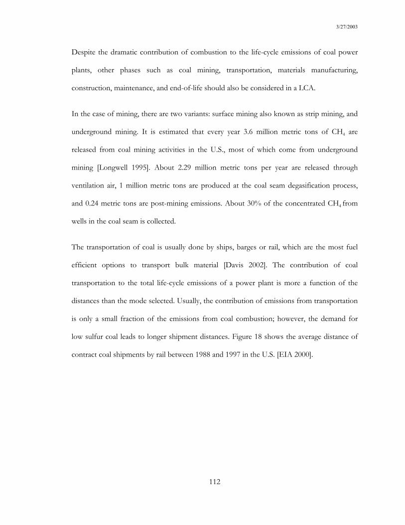
3/27/2003
112
Despite the dramatic contribution of combustion to the life-cycle emissions of coal power
plants, other phases such as coal mining, transportation, materials manufacturing,
construction, maintenance, and end-of-life should also be considered in a LCA.
In the case of mining, there are two variants: surface mining also known as strip mining, and
underground mining. It is estimated that every year 3.6 million metric tons of CH4 are
released from coal mining activities in the U.S., most of which come from underground
mining [Longwell 1995]. About 2.29 million metric tons per year are released through
ventilation air, 1 million metric tons are produced at the coal seam degasification process,
and 0.24 metric tons are post-mining emissions. About 30% of the concentrated CH4 from
wells in the coal seam is collected.
The transportation of coal is usually done by ships, barges or rail, which are the most fuel
efficient options to transport bulk material [Davis 2002]. The contribution of coal
transportation to the total life-cycle emissions of a power plant is more a function of the
distances than the mode selected. Usually, the contribution of emissions from transportation
is only a small fraction of the emissions from coal combustion; however, the demand for
low sulfur coal leads to longer shipment distances. Figure 18 shows the average distance of
contract coal shipments by rail between 1988 and 1997 in the U.S. [EIA 2000].
3/27/2003
113
0
200
400
600
800
1000
1200
1988 1989 1990 1991 1992 1993 1994 1995 1996 1997
Years
Ave
rage
Dis
tanc
e (m
iles)
Low Sulfur Medium Sulfur A Medium Sulfur B High Sulfur
Notes: Low Sulfur = less than or equal to 0.6 pounds of sulfur per million Btu; Medium Sulfur A = 0.61 to 1.25 pounds per million Btu;
Medium Sulfur B = 1.26 to 1.67 pounds per million Btu; High Sulfur = greater than 1.67 pounds per million Btu.
Figure 18: Average Distance of Coal Shipments by Rail in the U.S., 1988-1997 [U.S. EIA 2000]
In the case of technologies that demand lime or limestone for flue gas desulfurization, total
emissions produced during the transportation of such materials could be higher than total
emissions produced during coal transportation. In addition limestone production requires
considerable amounts of energy, and therefore its production is also responsible for CO2
emissions [Spath 1999]. The coal versus limestone ratio varies according to the power plant’s
technology. A Pulverized Fuel (PF) plant, for instance, has a 8:1 ratio of coal to limestone.
Some environmental regulations affecting coal power plants are significant in terms of their
CO2 emissions. For example, flue gas clean-up, which is used to remove sulfur emissions,
produces more CO2 emissions than other upstream processes [Spath 1999]. The process
3/27/2003
114
requires considerable loads of limestone, which are responsible for 59 to 62% of the non-
coal CO2 emissions of the average and NSPS systems respectively. Such emissions amount
to twice as much the emissions released from the transportation of the coal consumed by
these technologies. Alternatively the use of coal with lower sulfur content may incur in
additional emissions from coal transportation from longer distances compared to the range
of distances to obtain a higher sulfur content fuel.
The production and use of natural gas to regenerate the CuO absorber during the life-cycle
of the LEBS system releases 35% of the non-coal CO2 emissions [Spath 1999]. Coal
transportation to operate a LEBS power plant amounts to 40% of the non-coal CO2.
The contribution of the coal power plant construction phase to the life-cycle emissions is
minimal. Usually the LCAs report only the major construction materials, which are concrete
and steel. In addition, some sources also report the consumption of inputs used in the
operation of the power plant such as lime, limestone, natural gas, etc. (Table 18).
The capacity factor of a coal power plant affects the life-cycle emissions of the plant.
However, a higher capacity factor may lead to shorter life-time of some structures of the
power plant, and moreover, the importance of the fixed factors such as the construction of
the power plant is minimal regarding its contribution to GHGs emissions [Pacca 2002]
One concern in a LCA of coal power plants is the fugitive CH4 emissions from coal mining
and handling, which contain significant amounts of CH4. Emissions during mining depend
on the ranking of coal, depth of the mine, technology used, and other environmental
conditions [Hayhoe 2002]. Underground mines in the U.S. release 11.0 to 15.3 m3 CH4 per
metric ton of coal (0.67 Gg CH4/106 m3 CH4, assuming 20º C and a pressure of 1 atm
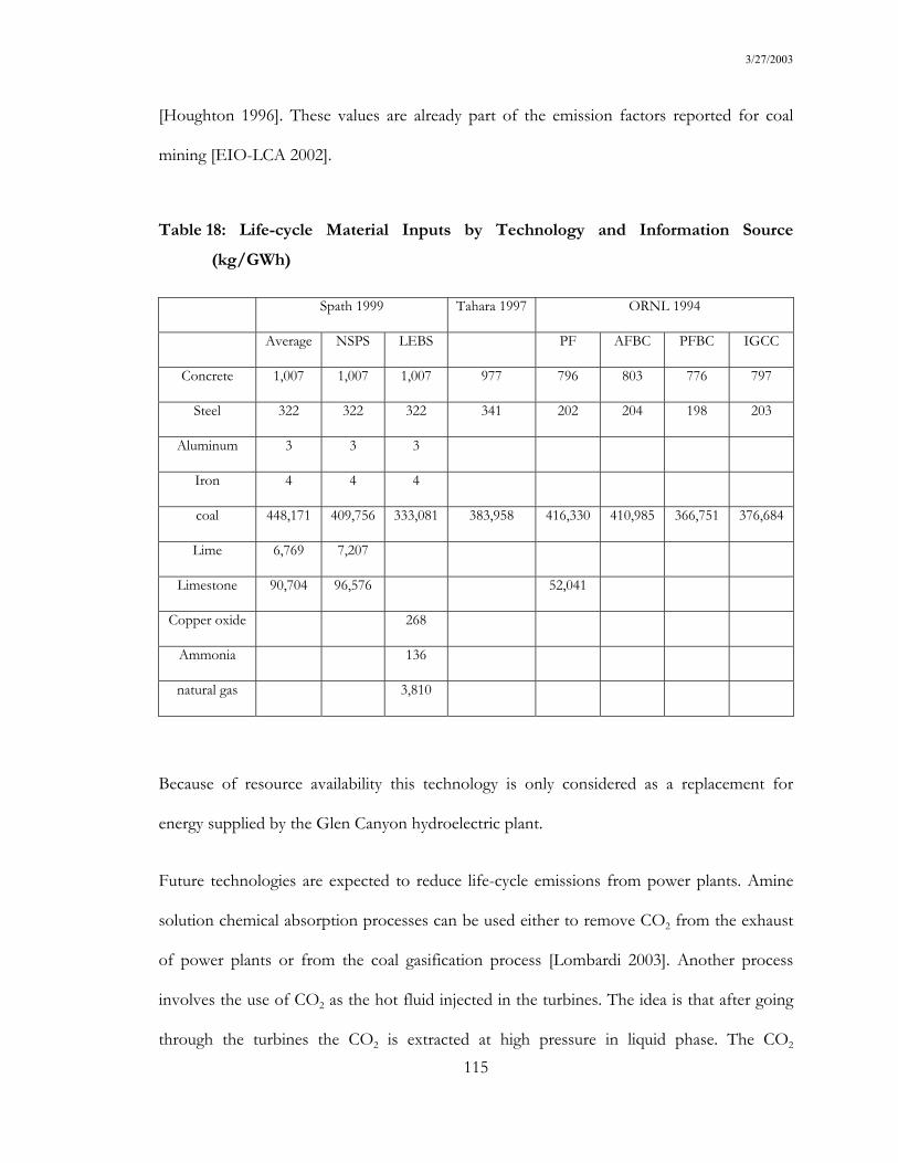
3/27/2003
115
[Houghton 1996]. These values are already part of the emission factors reported for coal
mining [EIO-LCA 2002].
Table 18: Life-cycle Material Inputs by Technology and Information Source
(kg/GWh)
Spath 1999 Tahara 1997 ORNL 1994
Average NSPS LEBS PF AFBC PFBC IGCC
Concrete 1,007 1,007 1,007 977 796 803 776 797
Steel 322 322 322 341 202 204 198 203
Aluminum 3 3 3
Iron 4 4 4
coal 448,171 409,756 333,081 383,958 416,330 410,985 366,751 376,684
Lime 6,769 7,207
Limestone 90,704 96,576 52,041
Copper oxide 268
Ammonia 136
natural gas 3,810
Because of resource availability this technology is only considered as a replacement for
energy supplied by the Glen Canyon hydroelectric plant.
Future technologies are expected to reduce life-cycle emissions from power plants. Amine
solution chemical absorption processes can be used either to remove CO2 from the exhaust
of power plants or from the coal gasification process [Lombardi 2003]. Another process
involves the use of CO2 as the hot fluid injected in the turbines. The idea is that after going
through the turbines the CO2 is extracted at high pressure in liquid phase. The CO2
3/27/2003
116
emissions from this technology are argued to be zero. This technology has not been
empirically demonstrated and the feasibility of the system needs to be proven considering
emissions from construction, maintenance, end-of-life, transportation, and storage of CO2
produced.
Coal combustion also releases black carbon (BC) and sulfur dioxide (SO2), which are
precursors to aerosol formation. The radiative forcing of such substances is not yet precisely
defined, but it is believed that they produce a cooling effect in the atmosphere [Hayhoe
2002].
4.4.1 Global Warming Effect of a Coal Fired Power Plant
A 1,000 MW coal-fired power plant with 6.08 TWh/year output [Tahara 1997] was scaled
down to 5.55 TWh to match Glen Canyon power plant output. The technology and design
of coal-fired power plants are not site-specific. Their environmental performance depends
on coal quality, firing configuration and technology type. Its location depends on the
availability of coal and cooling water. Since this alternative could replace energy from
hydropower, it could be installed close to the load center or the current power transmission
lines, and be accessible by railroad to deliver the coal.
It was assumed that after 30 years of operation all boilers had to be replaced (but not the
structure of the building), and that the required construction energy was 50% of the original.
The electricity output of the facility remained constant. The refurbishment resulted in 70,000
metric tons of CO2 emissions, one-third of the original emissions from manufacturing and

3/27/2003
117
constructing the plant (200,000 metric tons of CO2). As shown in Table 19, the GWE for
this power plant after 20 years of operation was estimated at 90,000,000 MTCO2Eq.
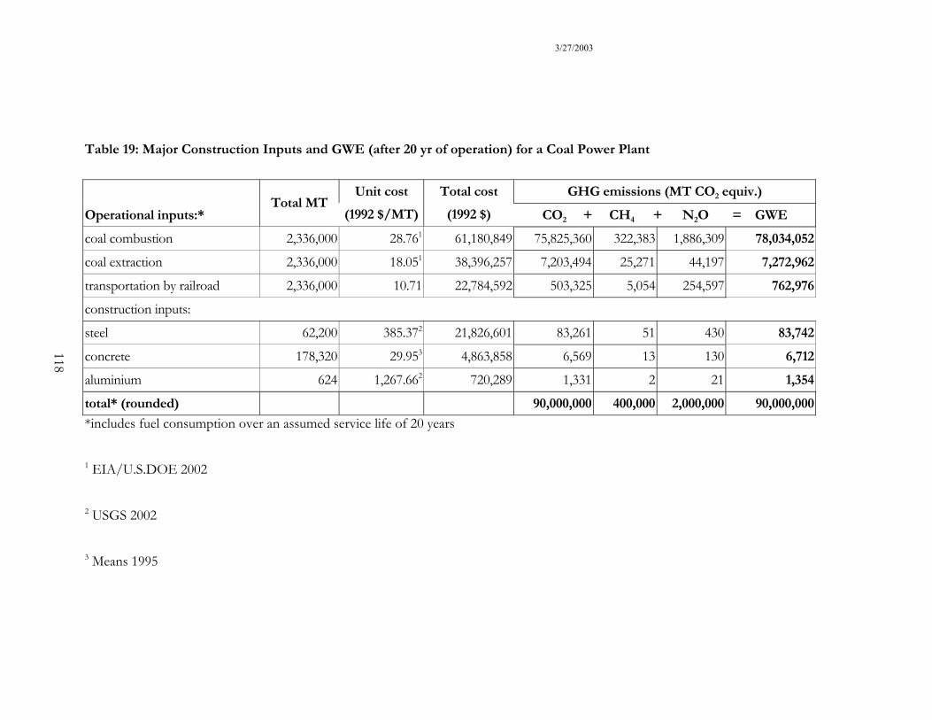
3/27/2003
Table 19: Major Construction Inputs and GWE (after 20 yr of operation) for a Coal Power Plant
GHG emissions (MT CO2 equiv.) Operational inputs:*
Total MT Unit cost
(1992 $/MT)Total cost (1992 $) CO2 + CH4 + N2O = GWE
coal combustion 2,336,000 28.761 61,180,849 75,825,360 322,383 1,886,309 78,034,052coal extraction 2,336,000 18.051 38,396,257 7,203,494 25,271 44,197 7,272,962transportation by railroad 2,336,000 10.71 22,784,592 503,325 5,054 254,597 762,976construction inputs:
steel 62,200 385.372 21,826,601 83,261 51 430 83,742concrete 178,320 29.953 4,863,858 6,569 13 130 6,712aluminium 624 1,267.662 720,289 1,331 2 21 1,354total* (rounded) 90,000,000 400,000 2,000,000 90,000,000*includes fuel consumption over an assumed service life of 20 years
1 EIA/U.S.DOE 2002
2 USGS 2002
3 Means 1995
118

3/27/2003
119
4.5 Natural Gas
Natural gas accounts for 22% of all energy consumed in the U.S., and its role in energy
production is becoming increasingly important due to environmental concerns. In
comparison with a coal-fired power plant a natural gas fueled power plant does not have the
problem of SO2 emissions and because the conversion to electricity is more efficient less
CO2 is emitted per unit of electricity output [Spath 2000]. In contrast to coal, natural gas is a
much more homogeneous fuel which is formed by 90% to 98% of pure methane and
contains 15 kg of carbon per GJ [Hayhoe 2002]. However, different natural gas turbine
technologies entail different efficiencies, heat rate, and consequentially different CO2
emissions. (Table 20).
Table 20: Performance of Natural Gas Generation Technologies [CEC 1997]
Natural Gas Generation Technology Fuel
Efficiency
Heat Rate
(Btu/kWh)
CO2 Reduction
Compared to
Baseline
Baseline: Steam Turbine 32% 10,666
Conventional Gas Turbine (simple cycle) 36% 9,508 11%
Conventional Gas Turbine (combined cycle) 51% 6,692 37%
ATS Gas Turbine (simple cycle) 43% 7,937 26%
ATS Gas Turbine (combined cycle) 60% 5,688 47%
Fuel Cell/Gas Turbine Hybrid 70% 4,876 54%
3/27/2003
120
Direct emission of particles is also minimal in a natural gas power plant compared to a coal-
fired power plant. However, some of the releases from natural gas handling and combustion
are also precursors for secondary particle formation in the atmosphere and some air
emissions contribute to the build up of GHGs in the atmosphere.
An assessment of the aggregated performance of the global electric system has shown that a
substitution of coal by natural gas initially leads to higher global temperatures compared to
the status quo. However, in the long run the world’s temperature is expected to decrease due
to lower CO2 and black carbon (BC) emissions. The time lag results from the continuous
production of aerosol precursors by coal power plants in contrast to the negligible
production of such precursors by natural gas-fueled power plants [Hayhoe 2002].
One concern in a LCA of natural gas power plants is the leaking of natural gas during
production and transportation, and the high rates of CH4 associated with such leaks. During
natural gas production 39,590 to 104,220 kg CH4/PJ natural gas may be released [Houghton
1996]. During natural gas processing, transport, and distribution 59,660 to 116,610 kg
CH4/PJ natural gas may be released. In the GWE method these emissions are taken into
account as they are already part of the emission factors reported in EIO-LCA for the sectors
“natural gas transportation” and “natural gas distribution” under the “transportation and
utility sector” [EIO-LCA 2002].
Table 21 shows published CO2 emissions for natural gas-fueled power plants. The range of
results is significant but most of the results converge to 400 to 600 g/kWh.
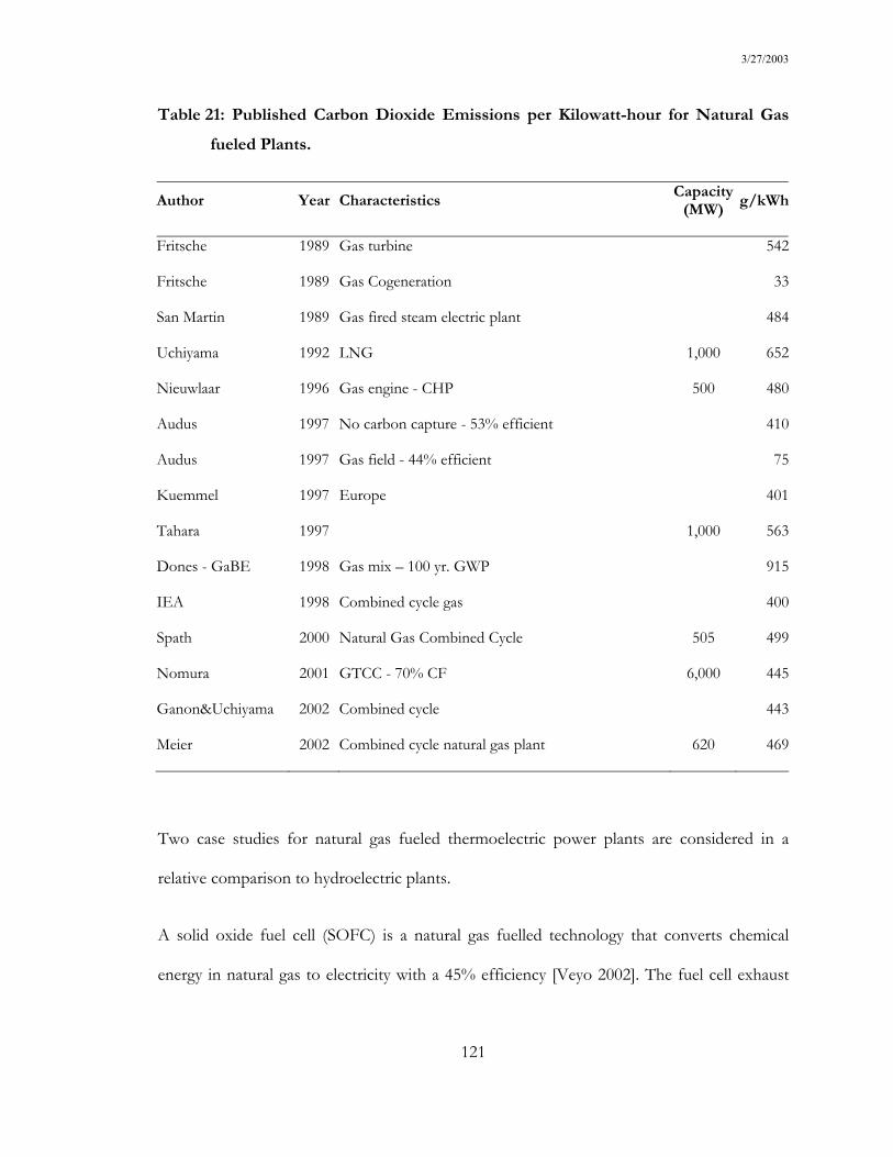
3/27/2003
121
Table 21: Published Carbon Dioxide Emissions per Kilowatt-hour for Natural Gas
fueled Plants.
Author Year Characteristics Capacity (MW) g/kWh
Fritsche 1989 Gas turbine 542
Fritsche 1989 Gas Cogeneration 33
San Martin 1989 Gas fired steam electric plant 484
Uchiyama 1992 LNG 1,000 652
Nieuwlaar 1996 Gas engine - CHP 500 480
Audus 1997 No carbon capture - 53% efficient 410
Audus 1997 Gas field - 44% efficient 75
Kuemmel 1997 Europe 401
Tahara 1997 1,000 563
Dones - GaBE 1998 Gas mix – 100 yr. GWP 915
IEA 1998 Combined cycle gas 400
Spath 2000 Natural Gas Combined Cycle 505 499
Nomura 2001 GTCC - 70% CF 6,000 445
Ganon&Uchiyama 2002 Combined cycle 443
Meier 2002 Combined cycle natural gas plant 620 469
Two case studies for natural gas fueled thermoelectric power plants are considered in a
relative comparison to hydroelectric plants.
A solid oxide fuel cell (SOFC) is a natural gas fuelled technology that converts chemical
energy in natural gas to electricity with a 45% efficiency [Veyo 2002]. The fuel cell exhaust
3/27/2003
122
temperature reaches 850ºC, and therefore, it can be coupled to a gas turbine. The overall
efficiency of the system reaches 60%.
4.5.1 Natural Gas Power Plant in the U.S.
Fuel switching such as the substitution of natural gas for coal is one of the most effective
ways currently available to reduce CO2 emissions [Hayhoe 2002].
The capacity of the facility used as a model for a natural gas power plant is 1,000 MW (6.34
TWh/year output scaled to Glen Canyon’s 5.55 TWh/year). The technology and design of
combined cycle gas turbines are not site specific. Its location depends on the availability of
natural gas and cooling water. If this alternative is to replace energy from hydropower, it
should be installed close to the load center or to the current power transmission lines.
It was assumed that after 30 years of operation all boilers had to be replaced (but not the
structure of the building), and that the required construction energy was 50% of the original.
The electricity output of the facility remained constant. The refurbishment resulted in 60,000
metric tons of CO2 emissions, about 60% of the original emissions from manufacturing and
constructing the plant (100,000 metric tons of CO2). As shown in Table 22, after 20 years of
operation, the GWE was estimated at 50,000,000 MTCO2Eq.
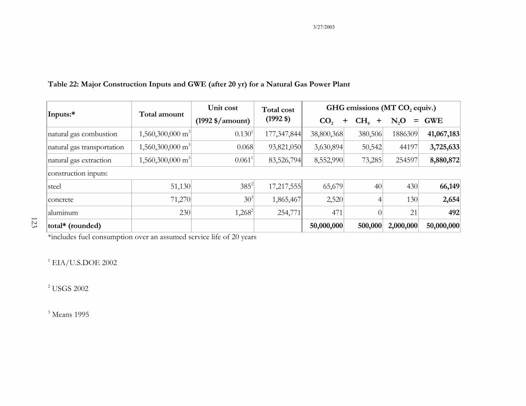
3/27/2003
Table 22: Major Construction Inputs and GWE (after 20 yr) for a Natural Gas Power Plant
Inputs:* Total amount Unit cost
(1992 $/amount)Total cost (1992 $)
GHG emissions (MT CO2 equiv.) CO2 + CH4 + N2O = GWE
natural gas combustion 1,560,300,000 m3 0.1301 177,347,844 38,800,368 380,506 1886309 41,067,183natural gas transportation 1,560,300,000 m3 0.068 93,821,050 3,630,894 50,542 44197 3,725,633natural gas extraction 1,560,300,000 m3 0.0611 83,526,794 8,552,990 73,285 254597 8,880,872construction inputs:
steel 51,130 3852 17,217,555 65,679 40 430 66,149concrete 71,270 303 1,865,467 2,520 4 130 2,654aluminum 230 1,2682 254,771 471 0 21 492total* (rounded) 50,000,000 500,000 2,000,000 50,000,000*includes fuel consumption over an assumed service life of 20 years
1 EIA/U.S.DOE 2002
2 USGS 2002
3 Means 1995
123
3/27/2003
124
4.5.2 Natural Gas Power Plant in Brazil
The capacity of the facility used as a model for a natural gas power plant is 1,000 MW (6.34
TWh/year output scaled to 49.4 TWh/year) [Tahara 1997]. In this idealized power plant we
assume that a conventional gas turbine with a simple cycle and a 36% efficiency is used. A
sensitivity analysis assuming the use of an Advanced Technology System (ATS) Gas Turbine
with a combined cycle and 60% of efficiency [CEC 1997].
It was assumed that after 30 years of operation all boilers had to be replaced (but not the
structure of the building), and that the required construction energy was 50% of the original.
The electricity output of the facility remained constant. The refurbishment resulted in
148,431 metric tons of CO2 emissions, about 55% of the original emissions from
manufacturing and constructing the plant (270,553 metric tons of CO2). As shown in Table
23, assuming 36% of efficiency after 20 years, the GWE was estimated at 420,000,000
MTCO2Eq. The use of the more efficient ATS would reduce the emissions to 250,000,000
MTCO2Eq (after 20 years).
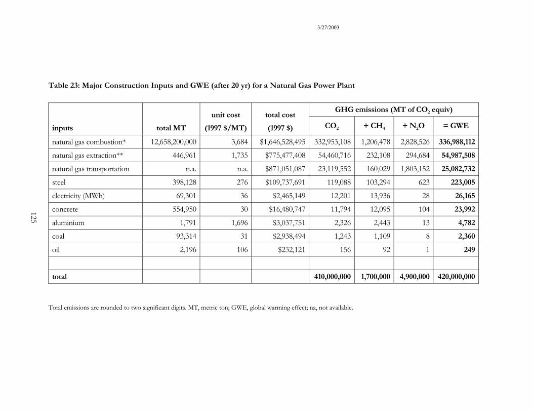
3/27/2003
Table 23: Major Construction Inputs and GWE (after 20 yr) for a Natural Gas Power Plant
GHG emissions (MT of CO2 equiv)
inputs total MT
unit cost (1997 $/MT)
total cost (1997 $) CO2 + CH4 + N2O = GWE
natural gas combustion* 12,658,200,000 3,684 $1,646,528,495 332,953,108 1,206,478 2,828,526 336,988,112natural gas extraction** 446,961 1,735 $775,477,408 54,460,716 232,108 294,684 54,987,508natural gas transportation n.a. n.a. $871,051,087 23,119,552 160,029 1,803,152 25,082,732steel 398,128 276 $109,737,691 119,088 103,294 623 223,005electricity (MWh) 69,301 36 $2,465,149 12,201 13,936 28 26,165concrete 554,950 30 $16,480,747 11,794 12,095 104 23,992aluminium 1,791 1,696 $3,037,751 2,326 2,443 13 4,782coal 93,314 31 $2,938,494 1,243 1,109 8 2,360oil 2,196 106 $232,121 156 92 1 249
total 410,000,000 1,700,000 4,900,000 420,000,000
Total emissions are rounded to two significant digits. MT, metric ton; GWE, global warming effect; na, not available.
125
3/27/2003
126
4.6 Problems from Dimensioning and Characterization of Power Plants
Besides the two problems described (LCA and GWP) earlier, there is also a third source of
problems which is how each of the electricity generation alternatives in a comparative
analysis is assembled and represented. There is a range of technologies and design options
for each alternative, which also need to be highlighted. Sometimes local conditions dictate a
given choice, especially in the case of renewable energy that relies on natural resources such
as insolation, wind distribution, water flows, topography, etc. In contrast, sometimes the
alternatives in a comparative analysis are selected and characterized based on objectives of
political considerations.
The selection of technologies within a given technology is also a key aspect. For example,
there are different types of PV modules with different energy conversion efficiencies,
lifetimes, and that require different material and energy inputs for its fabrication. Therefore,
it is important to keep in mind that a technology is not homogeneous. Along the same lines,
there are arch and gravity dams and the two designs also affect the performance of
hydroelectric plants.
Economies of scale also affect the performance of the alternatives. The size of a wind
turbine or a solar power plant affects the carbon emission intensity of the alternatives. The
load curve assumed to be met by electricity produced by a power plant also influences the
final result because sometimes some storage capacity could be necessary to match supply
and demand.
Finally, the lifetime assumed for a specific technology and the level of replacement that some

3/27/2003
127
of the parts are subject to also affects the outcome of the assessment. The end-of-life of
power plants suggests the recycling of part of the construction materials, which could be a
benefit in terms of GHGs emissions depending on the emissions from the recycling process
[Lombardi 2003].
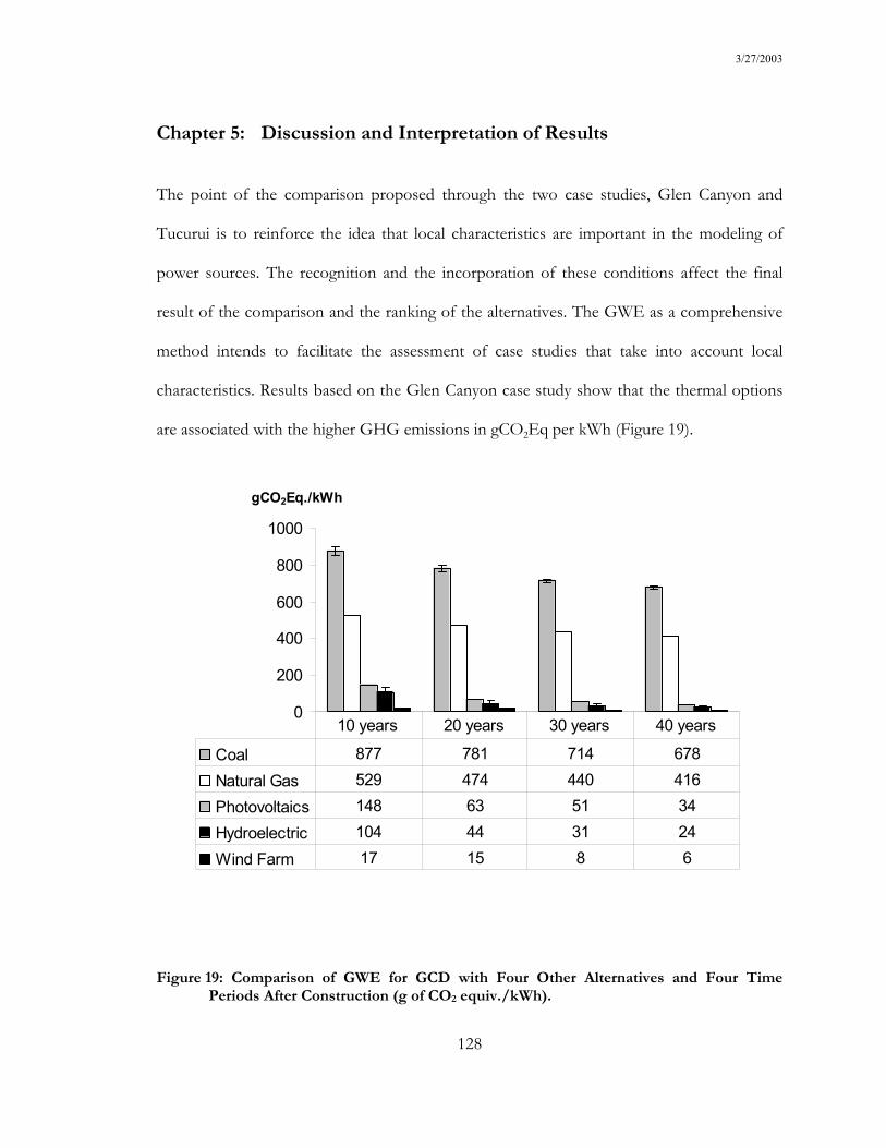
3/27/2003
128
Chapter 5: Discussion and Interpretation of Results
The point of the comparison proposed through the two case studies, Glen Canyon and
Tucurui is to reinforce the idea that local characteristics are important in the modeling of
power sources. The recognition and the incorporation of these conditions affect the final
result of the comparison and the ranking of the alternatives. The GWE as a comprehensive
method intends to facilitate the assessment of case studies that take into account local
characteristics. Results based on the Glen Canyon case study show that the thermal options
are associated with the higher GHG emissions in gCO2Eq per kWh (Figure 19).
Figure 19: Comparison of GWE for GCD with Four Other Alternatives and Four Time Periods After Construction (g of CO2 equiv./kWh).
0
200
400
600
800
1000
gCO2Eq./kWh
Coal 877 781 714 678
Natural Gas 529 474 440 416
Photovoltaics 148 63 51 34
Hydroelectric 104 44 31 24
Wind Farm 17 15 8 6
10 years 20 years 30 years 40 years
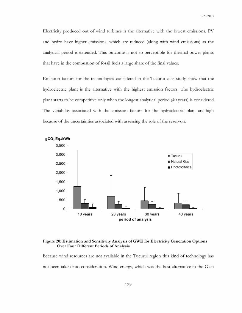
3/27/2003
129
Electricity produced out of wind turbines is the alternative with the lowest emissions. PV
and hydro have higher emissions, which are reduced (along with wind emissions) as the
analytical period is extended. This outcome is not so perceptible for thermal power plants
that have in the combustion of fossil fuels a large share of the final values.
Emission factors for the technologies considered in the Tucurui case study show that the
hydroelectric plant is the alternative with the highest emission factors. The hydroelectric
plant starts to be competitive only when the longest analytical period (40 years) is considered.
The variability associated with the emission factors for the hydroelectric plant are high
because of the uncertainties associated with assessing the role of the reservoir.
0
500
1,000
1,500
2,000
2,500
3,000
3,500
10 years 20 years 30 years 40 yearsperiod of analysis
gCO2 Eq./kWh
TucuruiNatural GasPhotovoltaics
Figure 20: Estimation and Sensitivity Analysis of GWE for Electricity Generation Options Over Four Different Periods of Analysis
Because wind resources are not available in the Tucurui region this kind of technology has
not been taken into consideration. Wind energy, which was the best alternative in the Glen

3/27/2003
130
Canyon case study, is not possible in this setting unless it is installed off site and the energy
is transmitted to the load area.
Most of the CO2 emissions from fossil fueled power plants account for annual emissions
from fuel combustion. Usually, this value depends on the annual electricity output of each
power plant and is assumed to be constant; therefore, it is possible to make a parallel
between the amount emitted by a fossil fuel plant and the amount corresponding to the
forgone NEP due to the footprint of a land-use intensive alternative such as a hydroelectric
plant or a massive PV installation. In this case, the NEP is also assumed to be constant over
a year even if in reality it depends on the exact ecosystem type, which varies over small areas,
and climatic conditions in a specific year.
Figure 21 shows such a comparison based on the three alternatives discussed, and the range
of assumptions considered for each one. In the case of the fossil fueled technology the
difference results from various technologies with different efficiencies. In the case of the PV
installation the difference arises from different technologies for module fabrication, which
also affect the efficiency of the devices. The lower CO2emissions estimation from the fossil
fueled power plant (133,000,000 MTCO2/yr) is twice as much as the foregone carbon
dioxide uptake due to the footprint of the hydroelectric plant (84,000,000 MTCO2/yr). The
worst case for PV (17,000,000 MTCO2/yr) is slightly over the best scenario for the
hydroelectric plant (14,000,000 MTCO2/yr).
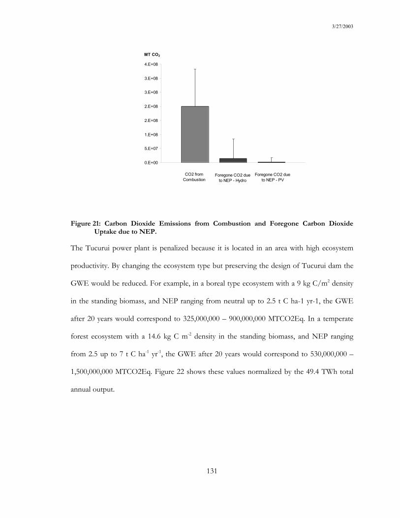
3/27/2003
131
Figure 21: Carbon Dioxide Emissions from Combustion and Foregone Carbon Dioxide Uptake due to NEP.
The Tucurui power plant is penalized because it is located in an area with high ecosystem
productivity. By changing the ecosystem type but preserving the design of Tucurui dam the
GWE would be reduced. For example, in a boreal type ecosystem with a 9 kg C/m2 density
in the standing biomass, and NEP ranging from neutral up to 2.5 t C ha-1 yr-1, the GWE
after 20 years would correspond to 325,000,000 – 900,000,000 MTCO2Eq. In a temperate
forest ecosystem with a 14.6 kg C m-2 density in the standing biomass, and NEP ranging
from 2.5 up to 7 t C ha-1 yr-1, the GWE after 20 years would correspond to 530,000,000 –
1,500,000,000 MTCO2Eq. Figure 22 shows these values normalized by the 49.4 TWh total
annual output.
CO2 from Combustion
Foregone CO2 due to NEP - Hydro
Foregone CO2 due to NEP - PV
0.E+00
5.E+07
1.E+08
2.E+08
2.E+08
3.E+08
3.E+08
4.E+08
MT CO2
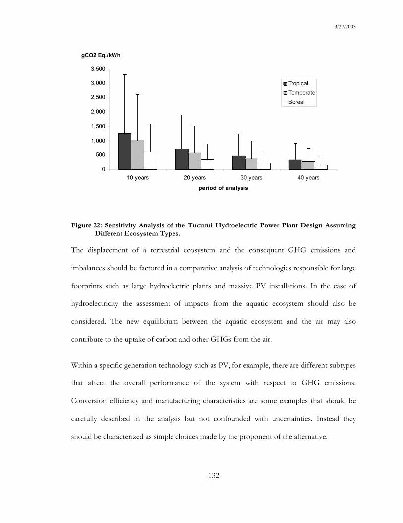
3/27/2003
132
0
500
1,000
1,500
2,000
2,500
3,000
3,500
10 years 20 years 30 years 40 years
period of analysis
gCO2 Eq./kWh
TropicalTemperateBoreal
Figure 22: Sensitivity Analysis of the Tucurui Hydroelectric Power Plant Design Assuming Different Ecosystem Types.
The displacement of a terrestrial ecosystem and the consequent GHG emissions and
imbalances should be factored in a comparative analysis of technologies responsible for large
footprints such as large hydroelectric plants and massive PV installations. In the case of
hydroelectricity the assessment of impacts from the aquatic ecosystem should also be
considered. The new equilibrium between the aquatic ecosystem and the air may also
contribute to the uptake of carbon and other GHGs from the air.
Within a specific generation technology such as PV, for example, there are different subtypes
that affect the overall performance of the system with respect to GHG emissions.
Conversion efficiency and manufacturing characteristics are some examples that should be
carefully described in the analysis but not confounded with uncertainties. Instead they
should be characterized as simple choices made by the proponent of the alternative.
3/27/2003
133
A methodological distinction when doing a LCA is the difference between choices and
uncertainty. While some criteria applied to the analysis are to the discretion of the analyst,
others reflect the incomplete knowledge about the true value of a parameter. An imprecise
measurement aggregates uncertainty in the analysis just as the estimations of parameters that
are difficult to assess with precision are also a source of uncertainties. Although sometimes
the analyst is forced to assume some values for parameters that are not precisely defined, this
practice is completely different than ignoring something that is known or selecting
alternatives among a set of available possibilities.
When assessing and comparing electricity generation technologies it is difficult to make
generalizations: each technology and each power plant has particular characteristics that
make them unique. For example, it is difficult to pick a number in the literature or analyze
particular case studies for hydroelectricity and generalize to all the hydroelectric plants in the
world. Depending on the ecosystem displaced the reservoir of a hydroelectric plant may
produce more or less emissions, as a function of the local climate, nutrient availability,
sediments, turbidity, water residence time, etc the productivity and consequent carbon burial
can be significant and offset part of the uptake associated with the dry land that existed
before the filling of the reservoir.
Accordingly, it is interesting to identify for each technology some characteristics that stand
out because of their effects on the final results.
3/27/2003
134
Chapter 6: Use of GWE in Environmental Policy and Management
Generally speaking the GWE method is offered to analysts who recognize that the selection
of electricity generation technologies for reduced climate change impacts is a fundamental
and necessary endeavor. Nonetheless, such action involves a set of assumptions, choices,
and uncertainties that affect the result of the assessment and are well portrayed by the GWE
framework.
Analysts carry out environmental assessments either to ratify a previously selected choice
that needs justification or because they are interested in the formulation of a new assessment
process and in achieving its refining to get the best outcome given an initial characterization
of the problem. The former practice is defined as position-focused whereas the latter is
known as the process-focused approach [Morgan 1990].
The GWE is a method that supports a process-focused analysis in the sense that the method
attempts to portray with transparency the problems associated with the analysis. However, it
would be naïve to neglect the existence of circularity between the definition and the
identification of problems. That is, depending on the definition used some problems could
be better identified than others, and depending on the identification of certain problems the
definitions could change. In any case, definition and identification of problems often vary
considerably depending on the circumstances of the analysis.
Accordingly, the GWE method is also designed for analysts that have a good knowledge
about the major components of the framework (LCA, GWP, electricity technologies/power
plants) and want to introduce modifications in the framework without losing the ability to

3/27/2003
135
interconnect these areas and tackle a specific problem. The GWE framework is flexible with
respect to the identification and definition of problems because we rarely know enough to
provide a definite answer to a problem, and the result from the analysis may be different
depending how a problem is perceived. The structure presented in section 3.2. to classify
and organize the problems arising from the use of each of the components of the GWE
method intends to motivate and guide the action of researchers that want to refine the
framework and obtain the best possible outcome.
Besides the flexibility arising from the transparency and the systematization of the sources of
problems in each of the components of the framework that invite the work of experts and
analysts willing to modify the assumptions, the GWE offers flexibility with respect to the
analytical period selected for each analysis. This feature is fundamental to support decision-
makers that usually demand answers in the short run (a couple of decades). In addition, due
to unexpected outcomes shorter analytical periods may be necessary to avoid an even greater
problem arising from global climate. Consequently, decision-makers interested in the
mitigation of climate change could benefit from the GWE framework to initiate programs
supporting technologies that reduce the burden of climate change over a time frame tailored
to their needs.
The choice of analytical periods transcending the “life-time” of a power plant is interesting
because it calls for the consideration of retrofits to extend the operation of the facilities. The
method is appropriate for analysis that span across individual life-time horizons because it
aggregates and weighs emissions over time.
Another use of the method is in the identification of a service or product's life-cycle phase

3/27/2003
136
that most contribute to the GWE given a chosen analytical time. Therefore, the method can
be used as a management tool to improve the performance of each technology. Examples of
energy technologies that benefit from such protocols are the use of renewable energy in the
manufacturing of PV modules and the life extension of hydroelectric plants, provided that
impacts from decommissioning of hydroelectric plants are constant after some time.
The GWE framework allows decision-makers to adopt a proactive approach towards the
mitigation of climate change. Although the framework is applied for electricity generation
options it could be used to compare alternatives within different sectors. The use of the
GWE decoupled from ultimate damages associated with climate change enhances the
method’s applicability since less assumptions and uncertainties are incorporated in the
assessment. Consequently, results can be more clearly presented to a broad audience.
1. relative comparison – ranking of alternatives
2. intermediate indicator avoid uncertainty to bridge emissions to changes in
temperature, and finally to actual impacts.
It was already discussed that transparency in the framework allows the communication of
uncertainties and problems that can be unbounded by the analyst. In addition the
representation of uncertainty and problems in the framework enhance the acceptability of
the framework as a decision-making tool. Representations of uncertainty in decision making
facilitate interaction between scientists and policy worlds and help to sustain the authority of
science [Shackley 1996]. Therefore, the quest for reduction of uncertainties does not
necessarily means the construction of more complex or powerful models representing the
real world but the use of simple interactive models that show clearly all uncertainties

3/27/2003
137
and assumptions involved in their formulation. If analysts communicate uncertainty well,
people has a clearer idea about what experts know and how experts disagree on the
formulations of uncertainties and problems.
The field of policy analysis needs to be concerned with the characterization and analysis of
uncertainty to an extent that far exceeds the need in the physical sciences audience because a
democratic decision process involves the input of various stakeholders who need to get their
views about the problem represented in the analytical process. Moreover, details in a
problem may change but the basic problem is the same it is important to be able to adapt,
use, policy analysis that have been done in the past. This task is easier when uncertainties
and problem are explicitly treated.
3/27/2003
138
Chapter 7: Dissertation Contribution
This dissertation describes means to achieve sensible climate change mitigation based on
current available energy technologies and at the same time it provides guidelines for
perfecting the performance of such technologies with respect to their impacts on global
climate change. That is, the method identifies the phases of a generation technology and the
GHG releases that produce the most significant GWE given a chosen analytical period. The
method intends to be an effective tool to assess and compare the potential impacts of energy
generation technologies over flexible analytical periods, which can be determined by the user
of the tool. Flexibility in the period of analysis strengthens the utility of the framework.
The choice of analytical periods transcending the “life-cycle” of a power plant is interesting
because it calls for the consideration of retrofits and upgrades to extend the operation of the
facilities. The method is appropriate for such analysis because it aggregates and weighs
emissions over time. Therefore, the method can be used as a management tool to improve
the performance of each technology. Examples of energy technologies that benefit from the
use of such protocol are the use of renewable energy in the manufacturing of PV modules
and the life-cycle extension of hydroelectric plants provided that impacts from
decommissioning of hydroelectric plants are constant after some time.
Flexibility is also fundamental to support decision-makers that usually demand answers in
the short run (a couple of decades). Moreover, due to unexpected outcomes shorter
analytical periods than the 100 year time horizon associated with GWP usually applied to
energy analyses may be necessary to avoid an even greater problem arising from global

3/27/2003
139
climate change.
The use of the framework presented herein can be extended to other services and goods.
The use of GWE decoupled from ultimate damages associated with climate change enhances
the method’s applicability since fewer assumptions and uncertainties are incorporated in the
assessment. Consequently, the framework allows for a more clear presentation to a broad
audience. Even if the GWE method is not directly used to establish a global emissions level,
its grand purpose is aligned with climate change mitigation. Three different approaches to
define environmental protection levels are usually proposed: the zero risk approach, the
balancing approach, and the technology based approach [Portney 2000]. The goal of the zero
risk approach is to avoid the occurrence of any adverse health effect. On the one hand such
approach seems sensible, on the other hand science and economics defy its actual
application. It may be difficult to specify a threshold based on scientific evidence, and it may
be impossible to keep an economic activity without producing environmental harm. The
balancing approach weighs competing outcomes and recommends regulatory action based
on the results. This approach has been presented in the discussion on BCA in this
dissertation. The problem is that economic analysis is ill prU.S. EPAred to convert a myriad
of non-market values into dollars. Finally, the technology-based approach characterizes the
maximum attainable pollution level based on the adoption by all sources of the best available
technology (BAT). A problem with this approach is that it is difficult to define the “best
technology” because emissions can always be further reduced at higher costs.
The GWE framework fits the class of technology-based approaches; however, it is more
flexible and powerful because despite being focused on a single service there are various
3/27/2003
140
technologies that can be considered for electricity generation. Moreover, the selection of one
technology over another is a function of a nexus of a variety of factors, which are
accommodated by the proposed framework. The framework also recognizes the variability
within a class of energy technologies. For example, different hydroelectric dam designs,
different PV system designs, as well as different scales, natural settings, etc, are accounted
for.
The framework intends to be flexible in order to house and transparently represent
variability. Because GWE is also useful to perfect each power generation technology
regarding their overall contribution to climate change, the definition of technology in the
framework is dynamic since it intends to transform current technologies into less polluting
options. The continuous utilization of the framework as a management tool could feed a
perpetual quest for sustainable energy technologies.
There is a considerable number of energy LCAs in the literature dealing with impacts on
climate change. They draw on different methods and assumptions to assess carbon dioxide
emissions from electricity generation projects. Some of these studies present the primary
information used to characterize a given power plant but rely on different assumptions and
methods to finally calculate the contribution of the power plants. Most studies that run
assessment of various GHGs use a fixed GWP to convert other GHGs to carbon dioxide
equivalents; and therefore, are locked to fixed time horizons. Such strategy may constrain the
use of the results and the comparison of different case studies. The use of the GWE
framework to process data available from other published sources is useful to normalize and
compare results without having to collect basic information about each project. This could

3/27/2003
141
be useful to set up a database with various projects with different characteristics for a given
power generation technology class and establish benchmarks for various alternatives.
Because the GWE method relies partly on EIO-LCA, which provides average emission
factors for the U.S. economy, it is a good tool to carry out comparisons of alternatives in the
U.S.. Nonetheless, the use of average values to characterize emissions from materials used in
the power plant should be contrasted with the use of specific information to portray
accurately the design and operation of a power plant.
Notwithstanding the power of the GWE method, the framework highlights the assessment
process as an active part of the results. The process is intended to be carefully explained in
this dissertation in order to enhance its replicability. As is presented there are three main
sources of problems associated with the GWE framework: (1) problems that arise from the
life-cycle assessment methods, (2) problems related to carbon cycle models and ways to
represent climate forcing of GHGs, (3) the diversity of various competing technologies,
settings, scales, life-times, maintenance options, available for a given power generation
technology.
To respond to such problems inherently associated with the framework but which are not
necessarily outcomes of uncertain knowledge about different components, the framework
attempts to be transparent. Consequently, the framework is implemented in a spreadsheet
tool that allows modification of different parameters in the analysis. Sensitivity analyses can
be performed parameter by parameter and values are subject to change at the discretion of
the user.
Since the establishment of the Intergovernmental Panel on Climate Change in 1988, climate

3/27/2003
142
change science has attempted to investigate different areas of anthropogenic activities such
as the ones represented in the IPCC special reports [Metz 2000, Nakicenovic 2000, Watson,
2000 Penner, 1999 Watson, 1997]. As a concept the GWE method attempts to bridge new
scientific understanding between GHGs in the atmosphere and terrestrial ecosystems that
are impacted by the footprint of large scale power plants such as a hydroelectric plant that
occupies a large parcel of land due to its reservoir. GWE incorporates land use change
information in the assessment of global climate change originating from the footprint of
energy generation technologies.

3/27/2003
143
Chapter 8: Future Work and Research Needs
A number of areas have been left unaddressed in this dissertation, and are available for
future work. For example:
1. perfecting the LCA model incorporating more specific process modeling
2. finding more specific information and data especially from the industrial sources that
manufacture the power generation equipment.
3. carrying out analysis of hybrid systems that involve the coupling of at least two electricity
generation technologies (e.g. hybrid systems)
4. comparing using more recent climate models (carbon cycle models) would be useful to
perfect the tool and update it with the latest scientific models.
5. adopting emission factors from other countries and add them to the model that currently
includes emission factors of the U.S. economy.
6. extending the GWE concept to incorporate land use change information that could be
related to a more precise assessment of the interactions between ecosystems change and
life-cycle impacts of energy technologies, especially models involving the balancing of
nitrous oxide.
7. assessing life-cycle emissions and climate forcing of other substances besides GHGs
such as aerosols.

3/27/2003
144
8. using a Monte Carlo Simulation with the various parameters in the assessment.
Only when the range of uncertainty is know or at least a given distribution can be associated
with this range it is possible to use some computational frameworks to analyze the
consequence of such variability in the final results of the assessment. Monte Carlo simulation
is an alternative to cope with uncertainties that propagates known parameter fluctuations
into an uncertainty distribution of the output variable.
Monte Carlo simulation is used to reveal the effects of uncertainties in the final results,
which requires the selection of specific statistical distribution functions for the uncertain
parameters. The logical association of the parameters is also selected by the analyst and the
output of the simulation produces a range of possible scenarios.
3/27/2003
145
Literature Cited
[Alsema 1998] Alsema, E.A., “Energy Requirements of Thin-film Solar Cell Modules - a review”, Renewable and Sustainable Energy Reviews, 2(4), pp. 387-415, 1998.
[Alsema 2000] Alsema, E.A. and E. Nieuwlaar, “Energy viability of photovoltaic systems”, Energy Policy, 28, pp. 999-1010, 2000.
[Alsema 2000b] Alsema, E.A., “Energy Pay-back Time and CO2 Emissions of PV Systems”, Progress in Photovoltaics: Research and Application, 8, pp. 17-25, 2000.
[Angelo 2002] Angelo, W.J., “First Offshore U.S. Wind Farm Expects Test Tower Permit”, Engineering News – Rec.ord (ENR), p. 16, July 2002.
[Arrenius 1896] Arrenius, S., "On the influence of Carbonic Acid in the Air upon the Temperature of the Ground”, The London, Edinburgh, and Dublin Philosophical Magazine and Journal of Science, pp. 237-276, April 1896.
[Audus 1997] Audus, H. and P. Freund, “The Costs and Benefits of Mitigation: A Full Fuel Cycle Examination of Technologies for Reducing Greenhouse Gas Emissions” Energy Conversion and Management, 38, pp. S595-S600, 1997.
[Bennett 2002] Bennett, D.H., T.E. McKone, J.S. Evans, W.W. Nazaroff, M.D. Margni, O. Jolliet, K.R. Smith, “Defining Intake Fraction”, Environmental Science and Technology, 36(9), pp. 206A–211A, May 2002.
[BLS 2002] U.S. Department of Labor, Bureau of Labor Statistics (2002) “Consumer Price Index (CPI)”, http://146.142.4.24/cgi-bin/surveymost?cu, Accessed December 2002.
[Bouwman 1990] Bouwman, A.F. (1990) “Exchange of Greenhouse Gases Between Terrestrial Ecosystems and the Atmosphere”, in: Bouwman A.F. (ed), Soils and the Greenhouse Effect. John Wiley, Chichester, UK, pp. 100-120.
[CEC 1998] California Energy Commission, “1997 Global Climate Change, Greenhouse Gas Emissions Reduction Strategies for California, Volume 2”, http://www.energy.ca.gov/global_climate_change/97GLOBALVOL2.PDF, Accessed January 2003, January 1998.
[Census 2003] U.S. Census “1997 Economic Census”, http://www.census.gov/epcd/ec97/introgen.htm, Accessed February 2003.
[Chamberland 1996] Chamberland, A. and S. Levesque, “Hydroelectricity, an Options to Reduce Greenhouse Gas Emissions from Thermal Power Plants”, Energy Conversion and Management, 37(6-8), pp. 885-890, 1996.
[Chapman 1974] Chapman P.F., G. Leach, M. Slesser, “Energy Budgets 2: Energy Cost of Fuels”, Energy Policy, 2(3), pp. 231-243, 1974.

3/27/2003
146
[Chapman 1975] Chapman, P.F. “Energy Analysis Of Nuclear-Power Stations”, Energy Policy, 3(4), pp. 285-289, 1975.
[Curran 1996] Curran, M. A., “Environmental Life-cycle Assessment”, New York, NY: McGraw-Hill Professional, 1996, ISBN 007015063X.
[Davis 2002] Davis, S.C. and S.W. Diegel, “Transportation Energy Data Book: Edition 22” Oak Ridge National Laboratory, September 2002.
[Dean 1998] Dean, W.E. and E. Gorham, “Magnitude and Significance of Carbon Burial in Lakes, Reservoirs, and Peatlands”, Geology, 26(6), pp. 535-538, 1998.
[Delmas 2001] Delmas, R., C. Galy-Lacaux, S. Richard, “Emissions of Greenhouse Gases from the Tropical Hydroelectric Reservoir of Petit Saut (French Guiana) Compared with Emissions from Thermal Alternatives”, Global Biogeochemical Cycles, 15(4), pp. 993-1003, 2001.
[Dones 1998] Dones, R. and R. Frischknecht, “Life Cycle Assessment of Photovoltaic Systems: Results of Swiss Studies on Energy Chains”, Progress in Photovoltaics: Research and Applications, 6(2), 117-125, 1998.
[Egre 2002] Egre, D., and J.C. Milewski, “The diversity of Hydropower Projects”, Energy Policy, 30, pp. 1225-1230, 2002.
[EIA 2000] U.S. Energy Information Administration “Energy Policy Act Transportation Rate Study”, Final Report on Coal Transportation, October 2000, http://www.eia.doe.gov/cneaf/coal/coal_trans/epact2000.html, Accessed February 2003.
[EIA 2002] U.S. Department of Energy, Energy Information Administration “Energy Prices”, Washington, D.C., 2002.
[EIA 2003] U.S. Energy Information Administration "Table C6 Gross Heat Content of Coal, 1991-2000" http://www.eia.doe.gov/emeu/iea/tablec6.html, Accessed February 2003.
[Einsele 2001] Einsele, G., J. Yan, M. Hinderer, “Atmospheric carbon burial in modern lake basins and its significance for the global carbon budget” Global and Planetary Change, 30, pp. 167–195, 2001.
[EIO-LCA 2002] Economic Input-Output Life Cycle Assessment 2003, Carnegie Mellon University, Green Design Initiative, http://www.eiolca.net, Accessed December 2003.
[Enting 1994] Enting, I.G., T.M.L. Wigley, M. Heimann, “Future Emissions and Concentrations of Carbon Dioxide: Key Ocean/Atmosphere/Land Analysis”, Commonwealth Scientific & Industrial Research Organization (CSIRO), Division of Atmospheric Research, Technical Paper nº 31, 120 p., 1994.
[Fearnside 2002] Fearnside, P.M. “Greenhouse Gas Emissions from a Hydroelectric Reservoir (Brazil’s Tucurui Dam) and the Energy Policy Implications” Water, Air, and
3/27/2003
147
Soil Pollution, 133, 69-96, 2002.
[Frankl 1998] Frankl, P., A. Masini, M. Gamberale, D. Toccaceli, “Simplied Life-cycle Analysis of PV Systems in Buildings: Present Situation and Future Trends”, Progress in Photovoltaics: Research and Applications, 6(2), pp. 137-146, 1998.
[Friedl 2002] Friedl, G. and Wüest, A. “Disrupting Biogeochemical Cycles – Consequences of Damming” Aquatic Science, 64, pp. 55–65, 2002.
[Fritsche 1989] Fritsche, U., L. Rausch, K.H. Simon, “Umweltwirkungsanalyse von Energiesystem” Gesamt-Emissions-Modell Integrierter Systeme (GEMIS), Oko-Institut, Darmstadt, 1989.
[Fthenakis 2000] Fthenakis, V.M. “End-of-life Management and Recycling of PV Modules”, Energy Policy, 28, pp. 1051-1058, 2000.
[Gabi 2003] GaBi 3 Software System for Life Cycle Engineering, Institute for Polymer Testing and Polymer Science (IKP), University of Stuttgart, http://www.pe-product.de/GABI/htdoc/home_englisch.htm2003, Accessed January 2002.
[Gagnon 1997] Gagnon, L., and J. van de Vate, “Greenhouse gas emissions from hydropower: The state of research in 1996” Energy Policy, 1997, 25(1), pp. 7-13.
[Gagnon 2002] Gagnon, L., C. Bélanger, Y. Uchiyama, “Life-cycle Assessment of Electricity generation options: The status of research in year 2001” Energy Policy, 30(14), pp. 1267–1278, 2002.
[Ganon 1993] Gagnon, L., and A. Chamberland, “Emissions from Hydroelectric Reservoirs and Comparison of Hydroelectricity, Natural-Gas and Oil” Ambio, 22(8), pp. 568-569, 1993.
[Greijer 2001] Greijer, H., L. Karlson, S.E. Lindquist, A. Hagfeldt “Environmental Aspects of Electricity Generation From a Nanocrystalline Dye Sensitized Solar Cell System”, Renewable Energy, 23, pp. 27-39, 2001.
[Haack 1981] Haack, B.N., “Net Energy Analysis of Small Wind Energy-Conversion Systems”, Applied Energy, 9(3), pp. 193-200, 1981.
[Hansen 1988] Hansen, J., I. Fung, A. Lacis, D. Rind, S. Lebedeff, R. Ruedy, G. Russel, P. Stone, “Global Climate Changes as Forecast by Goddard Institute for Space Studies 3-dimensional Model”, Journal of Geophysical Research, 93, pp. 9341-9364, 1988.
[Hansen 1998] Hansen, J., M. Sato, A. Lacis, R. Ruedy, I. Tegen, E. Matthews, “Climate Forcings in the Industrial Era”, Proceedings of the National Academy of Sciences, 95, pp. 12753-12758, 1998.
[Hayhoe 2002] Hayhoe, K., H.S. Kheshgi, A.K. Jain, D.J. Wuebbles, “Substitution of Natural Gas for Coal: Climatic Effects of Utility Sector Emissions” Climatic Change, 54,

3/27/2003
148
pp. 107–139, 2002.
[Hendrickson 1998] Hendrickson, C. T., A. Horvath, S. Joshi, L.B. Lave, “Economic Input-Output Models for Environmental Life-Cycle Assessment.” Environmental Science and Technology, 32(4), 184-91. 1998
[Herendeen 1981] Herendeen R.A., R.I. Plant, “Energy Analysis of Four Geothermal Technologies”, Energy 6(1), pp. 73-82, 1981.
[Hong 1994] Hong, B.D., E.R. Slatick, "Carbon Dioxide Emission Factors for Coal", Quarterly Coal Report, U.S. Energy Information Administration, Washington, D.C., January-April 1994, pp. 1-8, http://www.eia.doe.gov/cneaf/coal/quarterly/co2_article/co2.html, Accessed February 2003.
[Horvath 1998a] Horvath, A. and C.T. Hendrickson, “Steel-Reinforced Concrete Bridges: Environmental Assessment”, Journal of Infrastructure Systems, 111-117, 1998.
[Horvath 1998b] Horvath, A. and C.T. Hendrickson, “A Comparison of the Environmental Implications of Asphalt and Steel-Reinforced Concrete Pavements.” Transportation Research Record, 1626, pp. 105-113, 1998.
[Houghton 1990] Houghton, J.T., B.A. Callander, S.K. Varney, “Climate Change 1990: The Intergovernamental Panel on Climate Change Scientific Assessment”, Cambridge University Press, New York, NY, 100 p., 1990.
[Houghton 2001] Houghton, J. T., Y. Ding, D.J. Griggs, M. Noguer, P.J. van der Linden, X. Dai, K. Maskell, C.A. Johnson, “Climate Change 2001: the scientific basis”, Contribution of Working Group I to the Third Assessment Report of the Intergovernmental Panel on Climate Change, Intergovernamental Panel on Climate Change (IPCC), Cambridge University Press, New York, 881 p., 2001.
[Howarth 1990] Howarth, R. B. and R. B. Norgaard, “Intergenerational Resource Rights, Efficiency, and Social Optimality”, Land Economics, 66(1), pp. 1-11, 1990.
[Howarth 1992] Howarth, R. B. and R.B. Norgaard, “Environmental Valuation Under Sustainable Development”, American economic review, 82(2), pp. 473-477, 1992.
[Howarth 1995] Howarth, R. B. and R.B. Norgaard, “Intergenerational Choices Under Global Change”, Handbook of Environmental Economics, D. W. Bromley, ed., Blackwell, Oxford, UK, pp. 111-137, 1995.
[Howarth 2003] Howarth, RB “Catastrophic Outcomes in the Economics of Climate Change” Climatic Change, 56, pp. 257–263, 2003.
[IEA 1998] International Energy Agency (IEA), “Benign Energy? The Environmental Implications of Renewables”, International Energy Agency, Paris, 1998, http://www.iea.org/pubs/studies/files/benign/full/00-bene.htm, Accessed December

3/27/2003
149
2002.
[IEA 2000] International Energy Agency (IEA), “Retail Energy Prices in Selected Countries in US Dollars/Unit”, International Energy Agency, Paris, 2000.
[IEA 2000b] International Energy Agency (IEA) “Experience Curves for Energy Technology Policy”, International Energy Agency, Paris, 2000.
[Ito 2003] Ito, M., K. Kato, H. Sugihara, T. Kichimi, J. Song, K. Kurokawa, “A Preliminary Study on Potential for Very Large Scale Photovoltaic Power Generation (VLS-PV) System in the Gobi Desert from Economic and Environmental Viewpoints”, Solar Energy Materials & Solar Cells, 75, pp. 507–517, 2003.
[Jacobson 2003] Jacobson, A., Phd Candidate Energy and Resources Group, UC Berkeley. Personal Communication, 2003.
[Johnson 2003] Johnson, J., “Blowing Green”, Chemical & Engineering News, 81(8), pp. 27-30, 2003.
[Joos 2003] Joos, F. “PR model”, Index of /~joos/gwp_SAR: puls_ip90_sar.for, http://www.climate.unibe.ch/~joos/gwp_SAR/puls_ip90_sar.for, Accessed March 2003.
[Joos 2003b] Joos, F. “A Comprehensive Non-Linear Pulse Response Model For Simulations of the Anthropogenic CO2 Transient Coded In Fortran 90” http://www.climate.unibe.ch/~joos/prmodel/, Accessed March 2003.
[Kato 1998] Kato, K., A. Murata, K. Sakuta, “Energy Pay-back Time and Life-cycle CO2 Emission of Residential PV Power System with Silicon PV Module”, Progress in Photovoltaics: Research and Application, 6, pp. 105-115, 1998.
[Keoleian 1997] Keoleian, G.A., G. Lewis, “Application of Life-cycle Energy Analysis to Photovoltaic Module Design”, Progress in Photovoltaics: Research And Applications, 5, pp. 287-300, 1997.
[Keoleian 2003] Keoleian, G.A., G. Lewis, “Modeling the life-cycle Energy and Environmental Performance of Amorphous Silicon BIPV Roofing in the US”, Renewable Energy, 28, pp. 271-293, 2003.
[Koch 2002] Koch, F.H. “Hydropower – the politics of water and energy: Introduction and Overview”, Energy Policy, 30, 1207-1213, 2002.
[Komiyama 1996] Komiyama, H., K. Yamada, A. Inaba, K. Kato, “Life-cycle Analysis of Solar Cell Systems as a Means to Reduce Atmospheric Carbon Dioxide Emissions” Energy Conversion and Management, 37(6-8), 1247-1252, 1996.
[Kreith 1990] Kreith, F., and P. Norton, “The Potential of Renewable Energy to Reduce Carbon Dioxide Emissions” Proceedings, 1st World Renewable Energy Congress, vol. 5.,

3/27/2003
150
Pergamon Press, Oxford, 1990.
[Kreith 1990] Kreith, F., P. Norton, D. Brown, “A Comparison of CO2 Emissions from Fossil and Solar Power Plants in the United States”, Energy, 15(12), pp. 1181-1198, 1990.
[Krohn 1997] Krohn, S., “The Energy Balance of Modern Wind Turbines”, Windpower Note, 16 December 1997.
[Kuemmel 1997] Kuemmel, B., S.K. Nielsen, B. Sorensen, “Life-cycle Analysis of Energy Systems”, Roskilde University Press, Narayana Press, Gilling, Denmark, 1997.
[La Rovere 2000] La Rovere, E.L. and F.E. Mendes, F.E. “Tucurui Hydropower Complex Brazil”, WCD Case Study, Final Report, World Commission on Dams, Cape Town, South Africa, 2000, www.damsreport.org/docs/kbase/studies/csbrmain.pdf, Accessed January 2003.
[Lave 1995] Lave, L. B., E. Cobas, C. Hendrickson, F. C. McMichael “Using Input/Output Analysis to Estimate Economy-wide Discharges,” Environmental Science & Technology, 29(9), pp. 420A-426A, 1995.
[Leach 1975] Leach, G. “Net Energy Analysis – Is It Any Use?” Energy Policy, 3(4), pp. 332-344, 1975.
[Lemer 1996] Lemer, A.C. “Infrastructure obsolescence and design service life” Journal of Infrastructure Systems, 2 (4), pp. 153-161, 1996.
[Lenzen 2001] Lenzen, M., “Errors in Conventional and Input-Output-Based Life-cycle Inventories” Journal of Industrial Ecology, 4(4), pp. 127-148, 2001.
[Lenzen 2002] Lenzen, M. and J. Munksgaard, “Energy and CO2 life-cycle analyses of wind turbines review and applications”, Renewable Energy, 26, pp. 339–362, 2002.
[Lind 1982] Lind, R. C. “Introduction,” in: Discounting for Time and Risk in Energy Policy. Edited by F. R. Ruskin, Resources for the Future, Washington, DC, pp. 1-19, 1982.
[Lombardi 2003] Lombardi, L, “Life-cycle Assessment Comparison of Technical Solutions for CO2 Emissions Reduction in Power Generation", Energy Conversion and Management, 44, pp. 93–108, 2003.
[Longwell 1995] Longwell, J.P. and E.S Rubin, “Coal: Energy for the Future”, U.S. National Research Council, Committee on the Strategic Assessment of the U.S. Department of Energy’s Coal Program, National Academy Press, Washington, D.C., 1995.
[Means 1995] “R. S. Means Building Construction Cost Data”, R. S. Means Co., Kingston, MA, 1995.
[Meier 2002] Meier, P.J. “Life-Cycle Assessment of Electricity Generation Systems and Applications for Climate Change Policy Analysis”, Doctoral Dissertation, Fusion
3/27/2003
151
Technology Institute University of Wisconsin, Madison Wisconsin, August 2002.
[Meridian 1989] Meridian Corporation “Energy System Emissions and Materiel Requirements”, Meridien Corporation, Alexandria, VA, 1989.
[Metz 2000] Metz, B., O. Davidson, J.W. Martens, S. Van Rooijen, L. Van Wie Mcgrory “Methodological and Technological Issues in Technology Transfer”, Special Report of the Intergovernmental Panel on Climate Change, Cambridge University Press, UK, pp 432, 2000.
[Metz 2001] Metz, B., D. Ogunlade, R. Swart, J. Pan, “Climate Change 2001: Mitigation”,: Intergovernamental Panel on Climate Change, Cambridge University Press, New York, NY, 752p., 2001.
[Morgan 1990] Morgan, M.G. and M. Henrion, “Uncertainty: A Guide to Dealing with Uncertainty in Quantitative Risk and Policy Analysis”, Cambridge University Press, New York, NY, 1990.
[Mulholland 1982] Mulholland, P. J., and Elwood, J. W., “The Role of Lake and Reservoir Sediments as Sinks in the Perturbed Global Carbon Cycle”, Tellus, 34, pp. 490–499, 1982.
[Myhre 1998] Myhre, G., E.J. Highwood, K.P. Shine, F. Stordal, “New Estimates of Radiative Forcing Due to Well Mixed Greenhouse Gases” Geophysical Research Letters, 25, pp. 2715-2718, 1998.
[Nakicenovic 2000] Nakicenovic, N and R. Swart, “Emissions Scenarios. Special Report of the Intergovernmental Panel on Climate Change”, Cambridge University Press, UK, 570 p., 2000.
[NETL 2003] National Energy Technology Laboratory (NETL) “Clean Coal Technology. Post-project Assessments”, http://www.lanl.gov/projects/cctc/programs/documents/cctcMA2.pdf, Accessed February 2003.
[Nguyen 2002] Nguyen, M., L.A. Baker, P. Westerhoff, “DOC and DBP Precursors in Western US Watersheds and Reservoirs”, Journal of the American Water Works Association, 94(5), pp. 98-112, 2002.
[Niewlaar 1996] Niewlaar, E., E. Alsema, B. Van Engelenburg, “Using Life-cycle Assessments for the Environmental Evaluation of Greenhouse Gas Mitigation Options”, Energy Conversion and Management, 37(6-8), pp. 831-836, 1996.
[Nomura 2001] Nomura, N., A. Inaba, Y. Tonooka, M. Akai, “Life-cycle Emission of Oxidic Gases from Power-generation Systems”, Applied Energy, 68, pp. 215-227, 2001.
[NREL 1991] National Renewable Energy Laboratory (NREL), “Solar Radiation Data Manual for Flat-Plate and Concentrating Collectors”, National Renewable Energy Laboratory, Analytic Studies Division, Golden, CO, 1991.

3/27/2003
152
[O’ Neill 1993] O' Neill, J. “Ecology Police and Politics”, Routledge, New York, 1993.
[Oeschger 1983] Oeschger, H. and M. Heimann “Uncertainties of Predictions of Future Atmospheric CO2 Concentrations”, Journal of Geophysical Research, 88(C2), pp. 1258-1262, 1983.
[Oliver 2000] Oliver, M. and T. Jackson, T “The Evolution of Economic and Environmental Cost for Criystalline Silicon Photovoltaics”, Energy Policy, 28, pp. 1011-1021, 2000.
[OMB 2003] Office of Management and Budget (OMB) “OMB Circular No. A-94”, Office of Management and Budget, U.S. Presidency, http://www.whitehouse.gov/omb/circulars/a094/a94_appx-c.html, Accessed February 2003.
[ORNL 1994] Oak Ridge National Laboratory and Resources For the Future “External Costs and Benefits of Fuel Cycles”, 7 Volumes, ORNL/RFF, McGraw-Hill,Utility Data Institute, Washington, D.C., 1995
[Pacca 2002] Pacca, S. and A. Horvath, “Greenhouse Gas Emissions from Building and Operating Electric Power Plants in the Upper Colorado River Basin” Environmental Science and Technology, 36, pp. 3194-3200, 2002.
[Pearch 2002] Pearce, J.M. “Photovoltaics - A Path to Sustainable Futures” Futures, 34, pp. 663-674, 2002.
[Penner 1999] Penner, J.E., D.H. Lister, D.J. Griggs, D.J. Dokken, M. McFarland, “Aviation and the Global Atmosphere”, A Special Report of IPCC Working Groups I and III in collaboration with the Scientific Assessment Panel to the Montreal Protocol on Substances that Deplete the Ozone Layer, Cambridge University Press, UK, 373 p., 1999.
[PNNL 1986] “Wind Energy Resource Atlas of the United States”, Pacific Northwest National Laboratory, Solar Technical Information Program, Solar Energy Research Institute, Richland, WA, 1986.
[Proops 1996] Proops, J.L.R., P.W. Gay, S. Speck, T. Schroder, “The Lifetime Pollution Implications of Various Types of Electricity Generation” Energy Policy, 24(3), pp. 229-237, 1996.
[Rees 2003] Rees, W.E. “A Blot on the Land” Nature, 421(27), p. 898, 2003.
[Rosa 1994] Rosa, L.P. and R. Schaeffer “Greenhouse-Gas Emissions From Hydroelectric Reservoirs” Ambio, 23(2), pp. 164-165, 1994.
[Rosa 1995] Rosa, LP and. R. Schaeffer, “Global Warming Potentials: the Case of Emissions from Dams.” Energy Policy, 23(2), pp. 149-158, 1995.
[Rudd 1993] Rudd, J.W.M., R. Harris, C.A. Kelly, R.E. Hecky, RE “Are Hydroelectric Reservoirs Significant Sources of Greenhouse Gases?” Ambio, 22(4), pp. 246-248, 1993.
3/27/2003
153
[San Martin 1989] San Martin, R. L. “Environmental Emissions from Energy Technology Systems: the Total Fuel Cycle”, U.S. Department of Energy, Washington, D.C., 1989.
[Schleisner 2000] Schleisner, L. “Life-cycle Assessment of a Wind Farm and Related Externalities.” Renewable Energy, 20, pp. 279-88, 2000.
[Shackley 1996] Shackley, S. and B. Wynne, “Representing Uncertainty in Global Climate Change Science and Policy: Boundary-Ordering Devices and Authority”, Science Technology & Human Values, 21(3), pp. 275-302, 1996.
[Shi 1992] Shi, G “Radiative Forcing and Greenhouse Effect due to the Atmospheric Trace Gases. Science in China (Series B), 35, pp. 217-229, 1992.
[Sima Pro 2003] “SimaPro LCA Software Tool”, PRé Consultants bv, Plotterweg, Amersfoort, Netherland, http://www.pre.nl/simapro/default.htm, Accessed February 2003.
[Spath 1999] Spath, P.L., M.K. Mann, D.R. Kerr, “Life Cycle Assessment of Coal-fired Power Production”, National Renewable Energy Laboratory (NREL), Golden, CO, 1999.
[Spath 2000] Spath, P.L., M.K. Mann, “Life Cycle Assessment of a Natural Gas Combined Cycle Power Generation System”, National Renewable Energy Laboratory (NREL), Golden, CO, 2000.
[Srinivasan 1999] Srinivasan, S., R. Mosdale, P. Stevens, C. Yang, “Fuel Cells: Reaching the Era of Clean and Efficient Power Generation in the Twenty-First Century” Annual Review of Energy and the Environment, 24, pp. 281–328, 1999.
[St. Louis 2000] St. Louis, V.L., C.A. Kelly, E. Duchemin, J.W.M. Rudd, D.M. Rosemberg, “Reservoir Surfaces as Sources of Greenhouse Gases to the Atmosphere: A Global Estimate” Bioscience, 50(9), pp. 766-775, 2000.
[Staebler 1977] Staebler, D.L. and C.R. Wronski, “Reversible Conductivity Changes in Discharge-Produced Amorphous Si”, Applied Physics Letters, 31(4), pp. 292-294, 1977.
[Stallard 1998] Stallard, R.F., “Terrestrial Sedimentation and the Carbon Cycle: Coupling Weathering and Erosion to Carbon Burial”, Global Biogeochemical Cycles 12(2), pp.231-257, 1998.
[Stronberg 1998] Stronberg, J. and S. Virinder, “Government Procurement to Expand PV Markets”, Technical Report, Renewable Energy Policy Project, Washington, D.C., 1998.
[Svensson 1993] Svensson, B.S. and S.O. Ericson, “Does Hydroelectric Power Increase Global Warming” Ambio, 22 (8), pp. 569-570, 1993.
[Uchiyama 1991] Uchiyama, Y. “Energy Analysis of Power Generation Plants”, CRIEPI - Economic Research Center, Technical Report nº Y90015, 1991.
[Uchiyama 1992] Uchiyama, Y. (1992) “Total System Analysis of Greenhouse Effect from

3/27/2003
154
Power Generation Plants”, Energy Forum, 1992.
[Uchiyama 2002] Uchiyama, Y. (2002) “Present Efforts of Saving Energy and Future Energy Demand/supply in Japan, Energy Conversion and Management, 43, pp. 1123–1131, 2002.
[USBR 1970] U.S. Bureau of Reclamation, “Glen Canyon Dam and Power Plant”, Technical Record of Design and Construction, U.S. Bureau of Reclamation, Denver, CO, 1970.
[USBR 2001a] U.S. Bureau of Reclamation, “Glen Canyon Dam Facts”, U.S. Bureau of Reclamation, http://www.uc.usbr.gov/information/gcdfacts.html, Accessed June 2001.
[USBR 2001b] U.S. Bureau of Reclamation, “Bureau of Reclamation Generator Power Uprate Program”, Technical Report, U.S. Bureau of Reclamation, http://www.usbr.gov/power/data/uprate/uprate.htm, Accessed June 2000.
[USBR 2001c] U.S. Bureau of Reclamation, “Glen Canyon Power Plant”, U.S. Bureau of Reclamation, http://www.usbr.gov/power/data/sites/glencany/glencany.htm, Accessed June 2001.
[USGS 2002] U.S. Geological Survey “Minerals Information Publications and Data Products” U.S. Geological Survey, Mineral Resources Program, 2002, http://minerals.usgs.gov/minerals/pubs/, Accessed January 2002.
[Veyo 20002] Veyo, S.E., L.A. Shockling, J.T. Dederer, J.E. Gillett, W.L. Lundberg, “Tubular Solid Oxide Fuel Cell/Gas Turbine Hybrid Cycle Power Systems: Status”, Journal of Engineering for Gas Turbines and Power, 124, pp. 845-849, 2002.
[Voorspools 2000] Voorspools, K.R., E.A. Brouwers, W.D. D'haeseleer, "Energy Content and Indirect Greenhouse Gas Emissions Embedded in 'Emission Free' Power Plants: Results for the Low Countries" Applied Energy, 67, pp. 307-330, 2000.
[Vorosmarty 1997] Vorosmarty, C.J., K.P. Sharma, B.M. Fedete, A.H. Copeland, J. Holden, J. Marble, J.A. Lough, “The Storage and Aging of Continental Runoff in Large Reservoir Systems of the World” Ambio, 26(4), pp. 210-219, 1997.
[Watson 1997] Watson, R.T., M.C. Zinyowera, R.H. Moss, “The Regional Impacts of Climate Change: An Assessment of Vulnerability”, A Special Report of IPCC Working group II, Cambridge University Press, UK, 517 p., 1997.
[Watson 2000] Watson, R.T. “IPCC Special Report on Land Use, Land-Use Change and Forestry”, Intergovernmental Panel on Climate Change, United Nations Environmental Program, World Meteorological Organization, Cambridge University Press, Cambridge, UK, 375 p., 2000.
[WCD 2000] World Commission on Dams “Dams and Development: A New Framework for Decision-Makin”. World Commission on Dams, Earthscan Publications Ltd, Sterling, VA, 2000.
[WMO 1999] World Meteorological Organization, “Scientific Assessment of

3/27/2003
155
Ozone Depletion”, 1998, Global Ozone Research and Monitoring Project, World Meteorological Organization, Technical Report No. 44, Geneva, Switzerland, 1999.
[Zwiers 2002] Zwiers, F. “Climate change: The 20-year Forecast” Nature, 416, pp. 690-91, 2002.
Related Documents