Global Land Use Changes due to the U.S. Cellulosic Biofuel Program Simulated with the GTAP Model By* Farzad Taheripour Wallace E. Tyner Michael Q. Wang Final Version August 2011 *Farzad Taheripour and Wallace E. Tyner are Energy Economist and Professor of the Department of Agricultural Economics, Purdue University, and Michael Q. Wang is a senior scientist with the Center for Transportation Research, Argonne National Laboratory.

Welcome message from author
This document is posted to help you gain knowledge. Please leave a comment to let me know what you think about it! Share it to your friends and learn new things together.
Transcript

Global Land Use Changes due to the U.S. Cellulosic Biofuel Program Simulated with the GTAP Model
By*
Farzad Taheripour
Wallace E. Tyner
Michael Q. Wang
Final Version
August 2011
*Farzad Taheripour and Wallace E. Tyner are Energy Economist and Professor of the Department of Agricultural Economics, Purdue University, and Michael Q. Wang is a senior scientist with the Center for Transportation Research, Argonne National Laboratory.

2
Global Land Use Changes due to the U.S. Cellulosic Biofuel Programs Simulated
with the GTAP Model
1. Introduction
The land use consequences of US biofuel programs and their contributions to
GHG emissions have been the focal point of many debates and research studies in recent
years. However, most of these studies focused on the land use emissions due to first
generation biofuels such as corn ethanol, sugarcane ethanol, and biodiesel (e.g. [1, 2] [3,
4]). A quick literature review indicates that only a few attempts have been made to
estimate these emissions for second generation biofuels which convert cellulosic
materials into liquid fuels.
Gurgel, Reilly, and Paltsev [5] introduced two biomass energy sectors (Bios-
Electric and Bio-Oil) into a highly aggregated computational general equilibrium (CGE)
model, known as the MIT Emissions Prediction and Policy Analysis (EPPA), to evaluate land
use consequences of producing biofuels from biomass feedstocks. That model ignores first
generation biofuels, aggregates all agricultural products in one sector thereby over-
simplifying the competition for land among its alternative uses, and relies on an old data set
which represents the world economy in 1999. Those authors predicted that producing energy
from biomass requires a considerable amount of land, about 0.5 hectares per 1,000 gallons of
ethanol. They did not calculate the land use emissions due to production of energy from
cellulosic materials.
In a preliminary work, Tyner, Taheripour, and Han [6] used farm level and partial
equilibrium models and showed that producing ethanol from corn stover may have
insignificant land use implications. The authors also concluded that the US idled and
3
cropland pasture can support considerable volumes of biofuel production without imposing a
major impact on other crop activities on cropland.
More recently, the United States Environmental Protection Agency (EPA) released its
emissions assessments for alternative biofuels including ethanol produced from corn stover
and a dedicated crop (switchgrass) [7]. To provide these assessments, EPA mainly relied on
the FASOM and FARPRI partial equilibrium models to evaluate domestic and international
land use impacts of the US biofuel production targets. The simulation results obtained from
these models showed that producing ethanol from corn stover has insignificant land use
impacts. However, producing ethanol from switchgrass will cause major land use changes in
the US and other countries across the world. The EPA results indicated that producing 7.9
billion gallons of ethanol from switchgrass will increase global cropland area by about 3
million hectares, of which 1.7 million hectares will occur in the US. In addition, according to
the EPA estimates, producing ethanol from switchgrass will curb acreages of US soybeans,
wheat, hay, and a variety of other crops by 3.36 million hectares. The EPA results indicated
that producing ethanol from switchgrass reduces the US land use emissions, because
producing switchgrass deposits carbon into the soil. According to this report, producing
ethanol from switchgrass reduces GHGs by 2.5 kg CO2 equivalent per million BTU of
ethanol produced due to the land use changes and soil carbon sequestration within US (about
190 grams CO2 equivalent per gallon of ethanol). On the other hand, producing ethanol from
switchgrass causes about 15 kg CO2 equivalent per million BTU due to the land use changes
in the rest of the world (about 1,140 grams CO2 equivalent per gallon of ethanol). Hence,
according to the EPA report the net land use emissions of producing ethanol from
switchgrass are about 12.5 kg CO2 equivalent per million BTU (about 950 grams CO2 per
gallon of ethanol).

4
The existing limited literature on land use impacts of producing biofuels from crop
and forest residues provides enough evidence to confirm that producing these fuels from
agricultural and forest residues causes insignificant land use impacts. However, this picture is
cloudy for dedicated energy crops. As mentioned above, some studies argue that it is possible
to produce dedicated energy crops on marginal and idled croplands, and therefore it will not
cause significant land use impacts. On the other hand, other studies indicate that this
argument could be misleading and that producing dedicated crops could lead to major land
use changes.
Estimating the land use impacts of producing biofuels from dedicated energy crops is
more complicated in many ways than that from corn ethanol. Production of dedicated crops
for significant volumes of biofuels could alter relative prices of crops and their profitability
leading farmers to produce them on their existing active croplands or convert their idled or
marginal croplands (e.g. cropland pasture) to produce these crops. Even marginal lands are
often used in some way for livestock production, so that competition must be taken into
account. Given that these crops are not produced at a commercial level yet, and it is not clear
how farmers will react when they become profitable, it is important to provide a
comprehensive analytical framework to assess a wide range of alternative possible cases
which may come about in the future.
This paper provides an analysis of the land use changes induced by biofuel
production from cellulosic feedstocks. It develops an economy-wide computational general
equilibrium (CGE) model based on the modeling framework developed at Purdue
University’s Center for Global Trade Analysis Project (GTAP) to assess the land use
consequences of producing biofuels from cellulosic materials including corn stover and
dedicated energy crops. In particular, we extend the model developed in Tyner et al. [4],
known as GTAP-BIO-ADV, in several directions. The new model is based on the latest

5
version of GTAP database (version 7), which depicts the world economy in 2004. It handles
production, consumption and trade of the first and second generation biofuels, and its land
use components allow competition among traditional crops and dedicated energy crops for
idled land and cropland pasture.
In what follows we first describe the model and data changes in the following
sections:
• Introducing biofuels into the 2004 version 7 GTAP data base,
• Introducing advanced biofuels into the GTAP modeling framework,
• Land supply nesting structure,
• Adding greater flexibility in acreage switching among different crops in response to
price changes,
• Including an endogenous yield adjustment for cropland pasture in response to
changes in cropland pasture rent.
We describe each of these changes to the basic modeling and data structure. Details
of the changes are provided in the appendices A, B, and C. Then we introduce the
experiments which are designed to simulate the land use impacts of biofuels mandates.
Finally, we provide estimates for the land use implications of alternative biofuel pathways
(both ethanol and bio-gasoline) from corn, corn stover, miscanthus, and switchgrass and their
associated emissions.
2. Introducing Biofuels into the 2004 Version 7 of GTAP Database
The first version of GTAP-BIO database was built based on the GTAP standard
database version 6 which represented the world economy in 2001 [8]. That database
covers global production, consumption, and trade of the first generation of biofuels
including ethanol from grains (eth1), ethanol from sugarcane (eth2), and biodiesel (biod)

6
in 2001. Recently, version 7 of GTAP database, which depicts the world economy in
2004 was published [9]. However, this database does not include biofuel industries. To
take advantage of this new database we introduced global production, consumption, and
trade of first generation biofuels in 2004 into this database. In addition, we introduced
several new industries into the data base to expand the space of biofuel alternatives to
second generation of biofuels as well (see Appendix A). In particular, we introduced
three feedstock industries (Miscanthus, Switchgrass, and Corn stover) and six advanced
biofuel industries (Miscanthus bio-gasoline (AdvfB_Misc), Switchgrass bio-gasoline
(AdvfB_Swit), Corn stover bio-gasoline (AdvfB_Stover), Miscanthus ethanol
(AdvfE_Misc), Switchgrass ethanol (AdvfE_Swit), and Corn stover ethanol
(AdvfE_Stover)) into the database. Given that the advanced cellulosic biofuels are not yet
commercially viable, we assigned very small values to the production and consumption
of these biofuels in 2004 and we used the most updated information obtained from the
literature and expert inputs to define the production technologies for these industries. We
also updated the land use, land cover, and land rent headers of the new GTAP-BIO
database according to unpublished work done by Avetisyan, Baldos and Hertel [10].
These authors updated the GTAP land use and land cover data set to 2004. The steps and
processes which we followed to construct the new database are described in Appendix A
of this paper in detail. Here we briefly introduce its major specifications.
The new GTAP-BIO data set represents the world economy in 2004 and covers
69 groups of commodities (including biofuels and their byproducts), 67 industries, and
117 regions. In this paper we aggregated the new database to the commodity and regional
aggregation levels which are used in Tyner et al. [4] with minor modifications. Here we

7
collapsed regions, commodities, industries, and endowments into 19 regions, 43 groups
of commodities, 41 industries, and 22 groups of endowments. See appendix A of this
paper for more details. In this aggregation crops are aggregated into 8 groups (including
paddy rice, wheat, coarse grains, oilseeds, sugar crops, other crops, miscanthus, and
switchgrass), and biofuels are: ethanol from grains, ethanol from sugar crops, biodiesel
from oilseeds, ethanol from corn stover, ethanol from miscanthus, ethanol from
switchgrass, bio-gasoline from corn stover, bio-gasoline from miscanthus, and bio-
gasoline from switchgrass.
The energy content of bio-gasoline is assumed to be equal to the energy content of
conventional gasoline, and the energy content of ethanol is two-thirds that of
conventional gasoline. In the advanced biofuel sectors, conversion of cellulosic materials
to gasoline-like hydrocarbon fuels follows a thermochemical conversion technology, and
conversion of cellulosic materials to ethanol follows a biochemical pathway.
In addition to these new commodities we split the traditional food and vegetable
oil industries into new industries of food, feed, crude vegetable oil, refined vegetable oil,
and oilseed meals to better represent and model the links and interaction among these
industries with crops and biofuel. In the older version of GTAP-BIO database oilseed
meals were tradable indirectly through the feed industry. In the new version oilseed meals
are directly and indirectly tradable, meaning that the oilseed crushing industry
(represented by the crude vegetable oil industry) could sell its oilseed meal outputs to
domestic buyers (including livestock and the feed industries) and international markets.
This will help us to model production and trade of oilseed meals more accurately and is
more consistent with the actual operation of this industry.

8
The land use and land cover categories and definitions used in this dataset are
very similar to those in the old version. However, we revised the rent values we assigned
to each type of land to make them more consistent with independently available
information in this area. The previous model did not have physical outputs for cropland
pasture. Because cropland pasture will take on much more importance in this version, we
created output values that resulted in yields somewhat less than hay yields on cropland.
This was done for both the U.S. and Brazil. This change plays an important role in
analyzing the land use impacts of producing biofuels from dedicated energy crops.
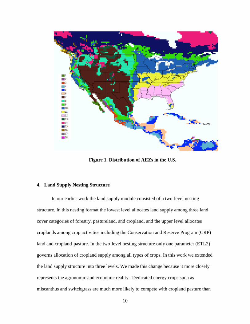
To introduce cellulosic biofuels we assumed that several regions including the
U.S., the EU and Brazil produce tiny volumes of cellulosic biofuels in the base year. For
the U.S. we assumed that miscanthus and switchgrass will be produced in AEZs 7 to 12,
mostly in AEZs 10, 11, and 12 (see Figure 1). These AEZs are endowed with large areas
of cropland pasture suitable for producing dedicated energy crops such as miscanthus and
switchgrass.
3. Introducing Advanced Biofuels into the GTAP Modeling Framework
To add second generation biofuels we adopt as the starting point for the new
model, the model reported in Tyner et al. [4] and known as GTAP-BIO-ADV. We made
several changes and modifications in the GTAP codes and its associated parameters to
introduce the advanced biofuels into GTAP modeling framework. These changes and
modifications are outlined in detail in Appendices A and B. Here we describe major
characteristics of the new model, which henceforth we refer to it as the GTAP-
BIO_ADVFUEL.
9
As noted earlier in this report, we first defined six industries to handle production
processes of the two new biofuels commodities – bio-gasoline and ethanol for each of the
three feedstocks. Then we introduced the new biofuels into the household demand
structure and the derived demand of firms for liquid fuels. To support production of the
new biofuels we defined three new industries (stover, miscanthus, and switchgrass)
which provide feedstocks for the new biofuel industries. The stover industry collects corn
stover and ships its output (collected corn stover) to the stover ethanol or bio-gasoline
industry. This industry uses inputs including fuel, fertilizer (to maintain productivity of
croplands where nutrients in stover are removed), transportation, capital, labor, and other
goods and services to collect, bail, store and ship corn stover to the stover processing
industry. The miscanthus and switchgrass industries are different from the stover
industry. These industries produce miscanthus or switchgrass and sell their products to
the processing industries. The miscanthus and switchgrass industries compete with crop
producers for cropland. It is important to note that we are not simulating miscanthus and
switchgrass together. We simulate either miscanthus or switchgrass, separately.
10
Figure 1. Distribution of AEZs in the U.S.
4. Land Supply Nesting Structure
In our earlier work the land supply module consisted of a two-level nesting
structure. In this nesting format the lowest level allocates land supply among three land
cover categories of forestry, pastureland, and cropland, and the upper level allocates
croplands among crop activities including the Conservation and Reserve Program (CRP)
land and cropland-pasture. In the two-level nesting structure only one parameter (ETL2)
governs allocation of cropland supply among all types of crops. In this work we extended
the land supply structure into three levels. We made this change because it more closely
represents the agronomic and economic reality. Dedicated energy crops such as
miscanthus and switchgrass are much more likely to compete with cropland pasture than
11
they are to compete with much more productive cropland used for corn, soybeans, etc.
Thus, the new structure better reflects what would likely emerge in this new production
activity. The lowest level of the new land supply model is the same as what we had
before. The second level divides cropland supply into two main crop categories. The first
group covers all traditional crops including rice, wheat, coarse grains, oilseeds, vegetable
and fruits, sugar crops, other crops, and CRP land (not used in this analysis). The second
group covers miscanthus, switchgrass, and cropland-pasture. The top level of this three-
level nesting structure determines supply of cropland to every crop activity. This nesting
structure allows us to assign different land transformation elasticities among the first and
second groups of crops (see Figure 3 in appendix B).
5. Adding Greater Flexibility in Acreage Switching Among Different Crops in
Response to Price Changes
In our previous work we and others observed that GTAP does not seem to have as
much acreage responsiveness as we experienced in the decade 2000-09. Indeed, it is the
case that in previous decades, crop acreages (distribution of cropland among alternative
crops) were much more responsive to changes in government programs, as these seemed
to be more important drivers than commodity prices. Chavas and Holt [11] used 1945-
1985 annual time-series data for U.S. corn and soybean acreage decisions, they found the
own-price elasticities for corn and soybeans to be very low, 0.158 and 0.441 respectively,
which were also confirmed by Gallagher [12], Lee and Helmberger [13], Tegene,
Huffman and Miranowski [14]. The small elasticities were due to the government
intervention in corn and soybean markets.

12
Houck and Ryan [15] evaluated the impact of government programs on corn and
concluded that more than 95% of variation in U.S. corn acreage during 1949-1969 can be
associated with variables that represent government intervention. Duffy, Kasazi and
Kinnucan [16] also used corn and soybean 1955-1988 annual time-series data to estimate
acreage response under farm programs. Their results showed that risk variability affected
soybeans to some extent but price variability in corn had little effect on planting
provisions due to extensive farm programs for corn to mitigate the effects of market
volatility. Houck and Subtonik [17], Chembezi and Womack [18], de Gorter and
Paddock [19], and Mclntosh and Shideed [20] also concluded that government programs’
impact on corn and soybean’s acreage response to be the most important one and
dominated other impacts. Clearly, prior to 2000, prices were less important in
determining acreage shifts. The GTAP parameter which governs the extent of acreage
shift among alternative cropping industries in response to relative crop prices was
calibrated on historical data. Given the recent observations on crop acreages, it seems that
farmers now respond to the relative crop prices more than what we observed in the past
(prior to 2000). In this analysis, we asked the question of whether there is any difference
in farmers reactions to crop price changes in the past decade and earlier periods. To
answer this question we estimated acreage response to changes in soybean and corn
returns per acre over different decades prior to 2000 and for 2000-2010. The following
regression shows the results for the time period of 2000-2010:
∆Harvesed corn area (acres) = 1.388 + 0.084 ∆Corn revenue/acre(t-1) – 0.138 ∆Soybean
revenue/acre(t-1)

13
The independent variable t values are 2.9 and 3.0 respectively, and the adjusted R2 is
0.44. For the 2000-2010 period, changes in corn and soybean revenues were a major
driver of changes in corn acres. We did the same regressions for prior periods and found
no significant relationship. As the literature suggests, in prior periods, government policy
was a major driver, and now it is commodity prices and revenue. For these reasons, we
increased the magnitude of the land supply transformation elasticity among the traditional
crops from -0.5 to -0.75. In the future, we will continue to test the sensitivity of this
parameter. A complete description of the new nesting structure and associated elasticities
is provided in Appendix B.
6. Endogenous Cropland Pasture Yield Change
Producing dedicated energy crops on cropland pasture will increase the
opportunity costs of using these lands as an input in livestock industry, which
consequently will lead farmers to improve productivity of their cropland pasture.
Cropland pasture today is used largely as an input to the livestock industry. We received
comments on our previous work suggesting that the increased use of land for biofuels
would lead to investments in increased productivity as land rents increased. This led us
to define a module to link productivity of cropland pasture with its rent. Rent is a residual
reflecting the underlying value of the land derived from its revenue streams. This module
determines changes in productivity of cropland pasture according to its rent and an
elasticity parameter which is added to the model parameters. This elasticity governs
cropland pasture yield change with respect to changes in the rent of cropland pasture.
The equation which represents the endogenous productivity increase is as follows:
),(]1[),( ripfriaf ϕβα ⋅+=

14
Where
Af(i, r): Cropland pasture augmenting technical change in Agro Ecological Zone i
of region r,
α: Scalar yield elasticity,
β: Scalar yield adjustment factor,
φ: Share of dedicated energy crop in total area of cropland pasture,
pf (i, r): Percent change in the rent of cropland pasture in Agro Ecological Zone i
in region r.
In the simulations presented in this report, we assigned a value of 0.4 to the scalar
yield elasticity (i.e. α=0.4) and assigned different values to the scalar yield adjustment
factor (β) to establish the following relationship between the area of cropland pasture
moved to the production of dedicated crops (ΔA) and the percentage change in the
average yield of cropland pasture (p_yield):
Ayieldp ∆= 15.4_ .
In other words, for each simulation, the value of β was calibrated to hold this relationship
constant. The productivity changes obtained from the scenarios which simulate the land
use impacts of producing biofuels from dedicated crops vary from about 15% for
miscanthus bio-gasoline to 35% for switchgrass ethanol.
Another interpretation of the productivity increase is that it is the productivity
increase required to obtain the land use change results provided in this report. In other
words, with no productivity increase, more land would be needed than is calculated with
the productivity increase. We have no clear empirical basis for the parameters used in
this analysis. As indicated above, we had clear and consistent feedback from reviewers

15
that by assuming no productivity increase, we were over-estimating the land use change.
Whether these results over or under estimate land use change associated with dedicated
energy crops is an open question.
7. Biofuel Scenarios for Simulation
To assess the land use emissions due to production and consumption of the second
generation of biofuels we defined the following seven experiments:
a. An increase in corn ethanol production from its 2004 level (3.41 billion gallons
[BG]) to 15 BG, using the 2004 database,
b. An increase in production and consumption of Bio-Gasoline produced from corn
stover (i.e. AdvfB-Stover) by 6 BG (or 9 BG ethanol equivalent), on top of 15 BG
corn ethanol,
c. An increase in production and consumption of Bio-Gasoline produced from
miscanthus (i.e. AdvfB-Misc) by 4.7 BG (or 7 BG ethanol equivalent), on top of
15 BG corn ethanol,
d. An increase in production and consumption of Bio-Gasoline produced from
switchgrass (i.e. AdvfB-Swit) by 4.7 BG (or 7 BG ethanol equivalent) on top of 15
BG corn ethanol,
e. An increase in production and consumption of ethanol from corn stover (i.e.
AdvfE-Stover) by 9 BG, on top of 15 BG corn ethanol,
f. An increase in production and consumption of ethanol from miscanthus (i.e.
AdvfE-Misc) by 7 BG, on top of 15 BG corn ethanol,

16
g. An increase in production and consumption of ethanol from switchgrass (i.e.
AdvfE-Swit) by 7 BG, on top of 15 BG corn ethanol.
These experiments are designed based on the targets which are defined in the Renewable
Fuel Standard (RFS2) and are explained in Appendix C.
8. Land Use Impacts
The land use impacts obtained from the experiments defined in the previous
section are presented in Table 1. This table indicates that producing 11.59 BG corn
ethanol increases global cropland area by 2.1 million hectares (0.18 hectares per 1000
gallons of ethanol). About 47% of this additional land requirement is expected to occur in
the U.S., and the share of forest in this land requirement is about 11%. In general, the
normalized additional land requirement obtained from this experiment (0.18) is in
between the corresponding figures reported for the second and third group of experiments
presented in Tyner et al. [4]. However, the share of forest in land conversion obtained
from the new experiment (11%) is smaller than the corresponding figures obtained from
the second and third groups of that report. Simulation results obtained from experiment
(a) indicates that also about 1.4 million hectares of cropland pasture will be converted to
cropland globally due to the corn ethanol shock. Cropland pasture is included in the
cropland cover classification. Cropland pasture is defined as land that as some point in
history was in cropland but is not today. It is not land considered converted from natural
land now. However, the data is available separately for this category, so alternative
assumptions can be applied. Cropland pasture land changes are reported in Table 2.
17
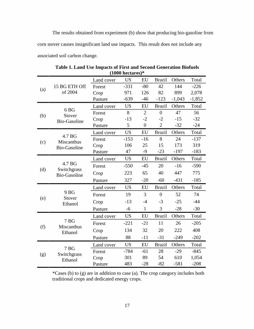
The results obtained from experiment (b) show that producing bio-gasoline from
corn stover causes insignificant land use impacts. This result does not include any
associated soil carbon change.
Table 1. Land Use Impacts of First and Second Generation Biofuels (1000 hectares)*
(a) 15 BG ETH Off of 2004
Land cover US EU Brazil Others Total Forest -331 -80 42 144 -226 Crop 971 126 82 899 2,078 Pasture -639 -46 -123 -1,043 -1,852
(b) 6 BG
Stover Bio-Gasoline
Land cover US EU Brazil Others Total Forest 8 2 0 47 56 Crop -13 -2 -2 -15 -32 Pasture 5 0 2 -32 -24
(c) 4.7 BG
Miscanthus Bio-Gasoline
Land cover US EU Brazil Others Total Forest -153 -16 8 24 -137 Crop 106 25 15 173 319 Pasture 47 -9 -23 -197 -183
(d) 4.7 BG
Switchgrass Bio-Gasoline
Land cover US EU Brazil Others Total Forest -550 -45 20 -16 -590 Crop 223 65 40 447 775 Pasture 327 -20 -60 -431 -185
(e) 9 BG
Stover Ethanol
Land cover US EU Brazil Others Total Forest 19 3 0 52 74 Crop -13 -4 -3 -25 -44 Pasture -6 1 3 -28 -30
(f) 7 BG
Miscanthus Ethanol
Land cover US EU Brazil Others Total Forest -221 -21 11 26 -205 Crop 134 32 20 222 408 Pasture 88 -11 -31 -249 -202
(g) 7 BG
Switchgrass Ethanol
Land cover US EU Brazil Others Total Forest -784 -61 28 -29 -845 Crop 301 89 54 610 1,054 Pasture 483 -28 -82 -581 -208
*Cases (b) to (g) are in addition to case (a). The crop category includes both traditional crops and dedicated energy crops.

18
Producing bio-gasoline from miscanthus requires a considerable amount of land
(in terms of new land plus cropland pasture moved to miscanthus). The result of
experiment (c) shows that producing 4.7 billion gallons of bio-gasoline from miscanthus
(equivalent to 7 BG ethanol) increases global cropland area (i.e. new cropland) by about
0.3 million hectares. About 33% of this new land requirement will occur in the US, and
globally forest has a share of 43% in this new land conversion. The normalized additional
land requirement of producing 4.7 BG bio-gasoline from miscanthus is about 0.07
hectares per 1000 gallons of bio-gasoline or 0.05 ha per 1000 gal. of ethanol equivalent,
considerably less than the requirement for corn ethanol. In general about 3.7 million
hectares of land are needed to produce 4.7 BG bio-gasoline from miscanthus. However,
this land requirement is mainly obtained from cropland pasture (see Table 2). To support
this shift the yield of cropland pasture would need to be increased by about 15%.
Producing miscanthus for biofuel transfers also some cropland pasture to production of
other crops and moderately affects allocation of cropland among crop activities.
The results from experiment (d) show that producing 4.7 BG of bio-gasoline from
switchgrass requires more land than miscanthus because the yield is considerably lower.
Global cropland area (i.e. new cropland) increases by about 0.8 million hectares, and
29% of that is in the US. Forest is 76% of the global total. The land requirement per
1000 gallons of bio-gasoline is 0.16 hectares (0.11 per 1000 gal. ethanol equivalent), less
than the requirement for corn ethanol, but much higher than miscanthus. About 7.1
million hectares of land is needed for switchgrass, as shown in Table 2 most of which
comes from cropland pasture. To support this shift the yield of cropland pasture would
need to be increased by about 29%. The large amount of land needed also explains why
19
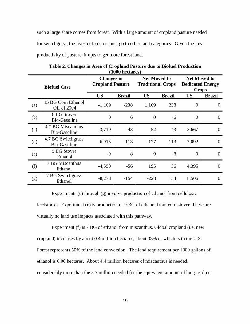
such a large share comes from forest. With a large amount of cropland pasture needed
for switchgrass, the livestock sector must go to other land categories. Given the low
productivity of pasture, it opts to get more forest land.
Table 2. Changes in Area of Cropland Pasture due to Biofuel Production (1000 hectares)
Biofuel Case
Changes in Cropland Pasture
Net Moved to Traditional Crops
Net Moved to Dedicated Energy
Crops US Brazil US Brazil US Brazil
(a) 15 BG Corn Ethanol Off of 2004 -1,169 -238 1,169 238 0 0
(b) 6 BG Stover Bio-Gasoline 0 6 0 -6 0 0
(c) 4.7 BG Miscanthus Bio-Gasoline -3,719 -43 52 43 3,667 0
(d) 4.7 BG Switchgrass Bio-Gasoline -6,915 -113 -177 113 7,092 0
(e) 9 BG Stover Ethanol -9 8 9 -8 0 0
(f) 7 BG Miscanthus Ethanol -4,590 -56 195 56 4,395 0
(g) 7 BG Switchgrass Ethanol -8,278 -154 -228 154 8,506 0
Experiments (e) through (g) involve production of ethanol from cellulosic
feedstocks. Experiment (e) is production of 9 BG of ethanol from corn stover. There are
virtually no land use impacts associated with this pathway.
Experiment (f) is 7 BG of ethanol from miscanthus. Global cropland (i.e. new
cropland) increases by about 0.4 million hectares, about 33% of which is in the U.S.
Forest represents 50% of the land conversion. The land requirement per 1000 gallons of
ethanol is 0.06 hectares. About 4.4 million hectares of miscanthus is needed,
considerably more than the 3.7 million needed for the equivalent amount of bio-gasoline
20
(experiment c). To support this large shift from cropland pasture to miscanthus
production an increase of 19% in the productivity of cropland pasture is needed.
Finally experiment (g) simulates production of 7 BG of ethanol from switchgrass.
It requires about 1 million hectares of new cropland globally (table 1), 29% of which is in
the US. Forest constitutes 80% of the converted land. The land requirement per 1000
gallons of ethanol is 0.15, close to the requirement for corn ethanol. Globally, 8.5 million
hectares of cropland pasture (table 2) are needed to support production of 7 BG of
ethanol from switchgrass. To support this large shift from cropland pasture to switchgrass
production, a sizeable increase of 35% in the productivity of cropland pasture is needed.
Table 3 summarizes the land needed per 1000 gallons of bio-gasoline or ethanol
for each of the cases. Three important conclusions emerge from this table. First,
switchgrass needs more land than miscanthus in all cases. This conclusion derives from
the assumed lower yield of switchgrass compared with miscanthus. Clearly, dedicated
energy crop yield is key to deriving the land use changes associated with these
feedstocks. Second, ethanol requires more land in all cases than bio-gasoline (in ethanol
equivalents) because the conversion efficiency is assumed to be higher for the
thermochemical process to produce bio-gasoline than for the ethanol bio-chemical
process. Third, both conversion processes produce negligible land use changes when corn
stover is the feedstock. The detailed land use changes among cropland, forest, and pasture
and in different global regions needed for GREET and other model applications are
available upon request from the authors.

21
Table 3. New Cropland Needed for the Different Cases
Biofuel Case
Biofuel Produced
(billion gallon)
New Cropland Needed
(1000 ha.)
New Cropland Needed
(ha./1000 gallons of biofuel)
New Cropland Needed
(ha./1000 gallons of ethanol eq.)
(a) Corn Ethanol 11.59 2078 0.18 0.18
(b) Stover Bio-gasoline 6 -32 -0.005 -0.004
(c) Miscanthus Bio-gasoline 4.7 319 0.07 0.05
(d) Switchgrass Bio-gasoline 4.7 775 0.16 0.11
(e) Stover Ethanol 9 -44 -0.005 -0.005
(f) Miscanthus Ethanol 7 408 0.06 0.06
(g) Switchgrass Ethanol 7 1054 0.15 0.15
9. Conclusions
These results suggest that corn stover (and by implication other crop residues)
have no significant induced land use change associated with biofuel production. The
results suggest that use of dedicated energy crops induces land use change and transfers
natural land (in particular forest) to crop production. Producing biofuels from dedicated
crops also transfers a major portion of cropland pasture to the production of these crops.
The size of this land transformation varies with the type of biofuel produced, and it
ranges between 16% and 35 % of the existing areas of US cropland pasture prior to
biofuel production. Our results indicate that producing bio-gasoline from miscanthus
generates the lowest land requirement across all alterative pathways which convert
dedicated crops to biofuels. This pathway needs about 0.07 hectares of new natural land

22
per 1000 gallons of bio-gasoline (or 0.05 hectares per 1000 gallons of ethanol
equivalent). The largest land requirement is associated with the switchgrass. This
pathway needs about 0.15 hectares of new natural land per 1000 gallons of ethanol. These
results indicate that the land requirements for switchgrass are considerably higher. The
difference is due largely to the assumed yields of switchgrass and miscanthus in this
analysis. If switchgrass yields turn out to be higher, then this difference would narrow.
These results indicate that recent articles which imply little or no land use impacts
from dedicated energy crops could be misleading. The land use impacts of producing
biofuels from dedicated crops is not zero because the opportunity costs of using cropland
pasture is not zero. Livestock producers will not give up their cropland pasture with no
compensation. The fact is that there is little completely idled land, especially in the U.S.
We have not used CRP acreage in these estimates. Also, these results for dedicated
energy crops depend upon the assumption of productivity increase in cropland pasture as
more and more of it is used for dedicated energy crops. We believe that some measure of
productivity increase is appropriate, but the magnitude needs more research.
In future research, we intend to present emission results of the simulated land use
changes using emission factors that are currently under development by our group and
others.
Acknowledgement: The authors are indebted to Jim Duffy (CARB), and Debo Oladosu
(ORNL) for very helpful comments on a previous draft of this paper. Partial funding for
the research effort at Purdue University was provided by Argonne National Laboratory
and the California Energy Commission.

23
References
1. Searchinger, T., et al., Use of U.S. croplands for biofuels increases greenhouse gases through emissions from land use change. Science, 2008. 319(5867): p. 1238-1240.
2. Taheripour, F., T. Hertel, and W.E. Tyner, Biofuels and Their By-Products: Global Economic and Environmental Implications. Biomass and Bioenergy, 2010. 34: p. 278-89.
3. Hertel, T., W. Tyner, and D. Birur, The Global Impacts of Multinational Biofuels Mandates. Energy Journal, 2010. 31(1): p. 75-100.
4. Tyner, W., et al., Land Use Changes and Consequent CO2 Emissions due to US Corn Ethanol Production: A Comprehensive Analysis, A Report to Argonne National Laboratory, 2010, Department of Agricultural Economics, Purdue University.
5. Gurgel, A., J.M. Reilly, and S. Paltsev, Potential Land Use Implications of a Global Biofuels Industry. Journal of Agricultural and Food Industrial Organization, 2007. 5: p. Article 9.
6. Tyner, W.E., F. Taheripour, and Y. Han., Preliminary Analysis of Land Use Impacts of Cellulosic Biofuels, Argonne National Laboratory and the California Energy Commission, Editor 2009.
7. U. S. Environmental Protection Agency, Renewable Fuel Standard Program (RFS2) Regulatory Impact Analysis, 2010: Washington, D.C.
8. Taheripour, F., et al., Introducing Liquid Biofuels into the GTAP Database, in GTAP Research Memorandum No 11, GTAP, Editor 2007, Purdue University: West Lafayette, IN.
9. Narayanan, B.G. and T.L. Walmsley, eds. Global Trade, Assistance, and Production: The GTAP 7 Data Base. 2008, Center for Global Trade Analysis, Purdue University.
10. Avetisyan, M., U. Baldos, and T. Hertel, Development of the GTAP Version 7 land Use Data Base, in GTAP Research Memorandum No. 192010, Purdue University: West Lafayette.
11. Chavas, J.-P. and M. Holt, Acreage Decisions under Risk: The Case of Corn and Soybeans. American Journal of Agricultural Economics, 1990. 72(3): p. 529-539.
12. Gallagher, P., The Effectiveness of Price Support: Some Evidence for U.S. Corn Acreage Response. Agricultural Economics Research, 1978. 30: p. 8-14.
13. Lee, R.R. and P.G. Helmberger, Estimating Supply Response in the Presence of Farm Programs. American Journal of Agricultural Economics, 1985. 67: p. 193-203.
14. Tegene, A., W.E. Huffman, and J.A. Miranowski, Dynamic Corn Supply Functions: A Model with Explicit Optimization. American Journal of Agricultural Economics, 1988. 70: p. 103-111.
15. Houck, J.P. and M.E. Ryan, Supply Analysis for Corn in the United States: The Impact of Changing Government Programs. American Journal of Agricultural Economics, 1972. 54(2): p. 184-191.
16. Duffy, P.A., S. Kasazi, and H.W. Kinnucan, Acreage Response Under Farm Programs for Major Southeastern Field Crops. Journal of Agricultural and Applied Economics, 1994. 26(2): p. 367-378.

24
17. Houck, J.P. and A. Subotnik, The U.S. Supply of Soybeans: Regional Acreage Functions. Agricultural Economics Research, 1969. 21: p. 99-108.
18. Chembezi, D.M. and A.W. Womack, Program Participation and Acreage Response Functions For U.S. Corn: A Regional Econometric Analysis. Review of Agricultural Economics, 1991. 13(2): p. 259-275.
19. de Gorter, H. and H. Paddock, The Impact of U.S. Price Support and Acreage Reduction Measures on Crop Output, in International Trade Policy Division1985, Agriculture Canada.
20. McIntosh, C.S. and K.H. Shideed, The Effects of Government Programs on Acreage Response Over Time: The Case of Corn Production in Iowa. Western Journal of Agricultural Economics, 1989. 41(1): p. 38-44.
21. Perkins, M., Brazil Biofuels Annual 2006, 2006, USDA/FAS Global Agricultural Information Network Report BR6008 Washington, D.C.
22. Huff, K., R. McDougall, and T. Walmsley, Contributing Input-OutputTables to the GTAP Data Base, GTAP Technical Paper Number 1, 2002.
23. Mielke, T., Oil World Annual 2006, 2006, ISTA Mielke Gmbh: Hamburg, Germany.
24. Miranowski, J. and A. Rosburg, An Economic Breakeven Model of Cellulosic Feedstock Production and Ethanol Conversion with Implied Carbon Pricing, 2010, Iowa State University: Ames, Iowa.
25. National Academy of Sciences, National Academy of Engineering, and National Research Council, Liquid Transportation Fuels from Coal and Biomass: Technological Status, Costs, and Environmental Impacts2009: National Academies Press.

25
Appendix A
Introducing the First and Second Generations of Biofuels into the GTAP Database Version 7
The first version of GTAP-BIO database was built based on the GTAP standard
database version 6 which represented the world economy in 2001 [8]. That database
covers global production, consumption, and trade of the first generation of biofuels
including ethanol from grains (eth1), ethanol from sugarcane (eth2), and biodiesel (biod)
in 2001.
This standard GTAP database version 7, recently published, also does not cover
biofuel industries. Following Taheripour et al. [8] we first introduce the first generation
of biofuels into this database. Then we define a process to introduce the second
generation of biofuels into this newer data base as well.
1. Introducing Biofuels into GTAP Version 7
To introduce eth1, eth2 and biod into the new database we replicate the original
work done by Taheripour et al. [8]. Hence in this section we briefly explain the steps
which we followed and the data items which we used. In addition, we highlight
differences between the new database and the original one.
1.1. Step One; Production and Trade of Biofuels in 2004
We collected data on consumption and trade of biofuels in 2004 from several
sources including the U.S. Department of Energy (DOE), the U.S. Department of
Agriculture (USDA), the Renewable Fuel Association (RFA), European Union of
Ethanol Producers, European Biodiesel Board, and others. Table A1 represents
production of grain-based ethanol, sugarcane-based ethanol, and biodiesel across the
world in 2004. Figures reported in this table are introduced into the GTAP-BIO database
version 7 as productions of eth1, eth2, and biodiesel in 2004.
In 2004 Brazil was the leading ethanol exporter in the world. Table A2 shows
2004 Brazilian exports. This data was introduced in the GTAP-BIO database version 7
for the trade of eht2. In this year trade of eht1 and biod were negligible.

26
Table A1. Global Biofuel Production in 2004 (million gallons)
Country Code in
GTAP V7 Country Name
Grain Based
Ethanol (eth1)
Sugarcane Based
Ethanol (eth2)
Biodiesel
BRA Brazil 0.0 3989.0 0.0 USA USA 3410.0 0.0 28.0 CHN China 100.5 0.0 0.0 ESP Spain 67.1 0.0 3.9 CAN Canada 52.8 0.0 0.0 IND India 0.0 42.5 0.0 FRA France 26.7 0.0 104.5 SWE Sweden 18.8 0.0 0.4 THA Thailand 0.0 14.8 0.0 POL Poland 12.7 0.0 0.0 ARG Argentina 0.0 8.4 0.0 XCB Caribbean 0.0 7.4 0.0 DEU Germany 6.6 0.0 310.7 AUS Australia 0.0 6.6 0.0 JPN Japan 6.2 0.0 0.0 PHL Philippines 0.0 4.4 0.0 NLD Netherland 3.7 0.0 0.0 LVA Latvia 3.2 0.0 0.0 FIN Finland 0.8 0.0 0.0 ITA Italy 0.0 0.0 96.1 DNK Denmark 0.0 0.0 21.0 CZE Czech Republic 0.0 0.0 18.0 AUT Austria 0.0 0.0 17.1 SVK Slovakia 0.0 0.0 4.5 BGR United Kingdom 0.0 0.0 2.7 LTU Lithuania 0.0 0.0 1.5
Sources: DOE, USDA, the Renewable Fuel Association, European Union of Ethanol Producers, and European Biodiesel Board.
1.2. Step Two; Sectors to Be Split and Biofuels Plant Level Models
Following the original work reported in Taheripour et al. [8], the new industries
of eht1, eth2, and biod are taken from the GTAP sectors of ofd, crp, and vol, respectively.
The production technologies of ethanol industries are also similar to our original work.

27
However, a new technology was introduced for biodiesel production. In the original
GTAP-BIO database the biodiesel industry was using oilseeds to produce biodiesel (as
the main product) and oilseed meal as the by-product. The biodiesel industry in the new
database uses crude vegetable oil and only produces biodiesel. Hence, in the new
database, the biodiesel industry does not produce any by-products. Instead, as explained
later on in this report, we defined a new industry which uses oilseeds to produce crude
vegetable oil and oilseed meals. The new approach models the role of oilseed meals in an
economy with biofuels more precisely.
Table A2. Brazil Ethanol Exports by Importing Countries
(million gallons)
Country Code in GTAP V7 Country Name Imports from
Brazil
CHL Chile 0.5 CRI Costa Rica 30.5 XCA El Salvador 7.5 IND India 125.1 XCB Jamaica 35.1 JPN Japan 58.4 MEX Mexico 1.0 NLD Netherlands 43.6 NGA Nigeria 28.2 XSM Others 68.5 KOR South Korea 72.8 SWE Sweden 44.0 TUR Turkey 3.2 USA U.S.A. 111.0 VEN Venezuela 0.1
Total 629.671
Source: [21]
While the cost structure of the eth1, eth2, and biod activities are the same as
before, their levels are tuned to the price levels of 2004. For the revenue side we assume
that the price of ethanol was about $1.69 per gallon (this was the US average ethanol
price in 2004). The price of biodiesel is determined according to its energy content
28
compared with the energy content of ethanol. In constructing the new database we take
into account the following subsidies and tariffs as well:
- U.S. ethanol subsidy of 0.51 cents per gallon,
- U.S. biodiesel subsidy of 100 cents per gallon,
- US ethanol tariff (2.5% ad valorem plus 54 cents/gal. specific),
We sequentially used the SplitCom program to split the original and parent sectors
of ofd, crp, and vol to the new sectors of eth1, eth2, biod, ofdn, crpn, and voln. These
processes are explained in detail in Taheripour et al.[8]. Table A3 represents global
production of biofuels introduced.
1.3. Split of Ethanol Between the Additive and Final Fuel
In this step we split ethanol consumption between two parts: ethanol as an
additive to gasoline and ethanol as a fuel extender. Following the original work we
assigned 75% of ethanol production to the additive role and the rest as a fuel consumed
by consumers. The database obtained from the above steps corresponds to the GTAP-
BIO version 6. Henceforth we refer to this database as GTAP-BIO_V7. This database
will be available for GTAP users. In the next sections we describe the modifications to
the commodity structure to better highlight the links among the crop, biofuels, food, feed,
and livestock industries.
2. Split of Standard GTAP Food Industry into Food and Feed Industries
In the GTAP-BIO databases the ofdn industry1 covers production of all processed
foods and animal feeds [22]. This aggregated industry has major forward and backward
links with many industries. It buys raw materials from crop, livestock, processed
livestock, and vegetable oil industries and sells its products to several sectors as
intermediate inputs and to households as final products. Indeed the ofdn covers two major
industries of processed food and processed feed. To better understand the implications of
biofuel production for these industries we split the ofdn industry into two distinct
activities of “food” and “feed”. To accomplish this task we pursued the following
assumptions and steps:
1 This sector is known as ofd in the GTAP standard database.

29
Table A3. Monetary Values of Outputs of Food and Feed Industries in GTAP-BIO V7 at
Market Prices (U.S. million dollars) Region* Food Feed
1 USA 247,252 41,246 2 EU27 732,996 62,195 3 BRAZIL 26,513 3,617 4 CAN 25,271 4,152 5 JAPAN 151,209 16,371 6 CHIHKG 67,136 20,259 7 INDIA 27,405 2,064 8 C_C_Amer 62,133 5,248 9 S_o_Amer 29,358 5,115 10 E_Asia 21,988 5,702 11 Mala_Indo 20,877 3,161 12 R_SE_Asia 21,083 2,802 13 R_S_Asia 4,474 887 14 Russia 15,400 2,701 15 Oth_CEE_CIS 24,667 2,892 16 Oth_Europe 18,983 1,660 17 MEAS_NAfr 27,062 3,185 18 S_S_AFR 28,008 3,626 19 Oceania 21,886 2,331 Total 1,573,701 189,213
* Members of these regions are shown in Table A10.
a. All sale items of the ofdn industry to the livestock industries (i.e. ctl, oap, rmk,
and wol) are assumed to be processed feed products. These items are
considered as sales of the feed industry. We applied the same rule for the
imported sales as well.
b. According to the very detailed U.S. 1997 input-output table obtained from
The Bureau of Economic Analysis of the U.S. Departments of Commerce, we
defined column shares to split the intermediate and primary inputs used by the
ofdn industry between the food and feed industries.
Given these assumptions we defined column, row, and cross shares for the
splitting process in each region. We introduced the column, row and cross shares into the
Split.com program to split the ofdn industry into two new industries. We allowed the

30
Split.com program to determine the trade shares as the residual. Table A3 represents the
monetary values of outputs of these new industries at market prices by region in the new
database.
3. Split of Standard GTAP Vegetable Oil Industry into Crude and Refined
Vegetable Oil Industries
In the GTAP-BIO database the “voln” industry2 covers production of all types of
vegetable oils and fats (for details see Karen Huff et al., 2000). This industry produces
crude and refined vegetable oils; animal and vegetable fats; and all types of oilseed
meals, oil cakes, and other residues resulting from the extraction of vegetable oils and
fats. This industry buys all types of oilseeds and animal fats along with other inputs and
sells its products mainly to the livestock and processed livestock industries, food
industries, processed animal feed industries, chemical industries, services (restaurants and
fast food), and households. In an economy with biofuels, the vol industry interacts with
the biofuel industry as well.
To better represent the forward and backward links between crop, vegetable oil,
livestock, food, feed and biofuel industries and follow the stream of commodities among
these industries, we split the voln sector into two distinct industries of crude vegetable oil
(cvoln) and refined vegetable oil (rvoln). The former industry crushes oilseeds and
produces two commodities: crude vegetable oil and oilseed by-products. The latter
industry uses crude vegetable oil and produces refined vegetable oil. To divide the voln
industry into the new sectors we pursued the following steps and assumptions:
a. All sale items of the voln industry to the livestock and feed industries (i.e. ctl,
oap, rmk, wol, and feed) are assumed to be animal feed. These items are
mainly oilseed meals, oil cakes, and other residues resulting from the
extraction of vegetable oils and fats. These items are considered as sales of the
cvoln industry. We applied the same rule for the imported sales as well.
b. The self use of the voln industry (mainly crude vegetable oil) is considered as
an intermediate input for the rvoln industry. This item is also included in the
sale items of the cvoln industry.
2 This sector is known as vol in the GTAP standard database.

31
c. In biodiesel producing regions, sales of vol to the biodiesel industry are
transferred to the cvoln industry.
d. All crop and livestock commodities purchased by the vol industry are
transferred to the cvoln industry.
e. Other cost items of the voln industry are mainly divided between the cvoln
and rvoln based on the sale shares of these two industries in total sale of the
voln industry. In some cases we modified the cost shares according to the cost
shares obtained from the U.S. input-output table.
Given these assumptions we defined column, row, and cross shares for the split
process in each region. We introduced the column, row and cross shares into the
Split.com program to split the voln industry into two new industries. We allowed the
Split.com program to determine the trade shares as the residual. In some cases we altered
the trade shares to match the results with real observation obtained from the Oil World
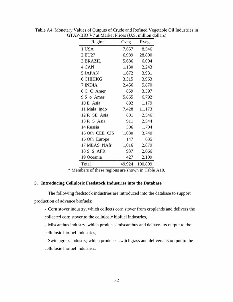
database [23]. Table A4 represents the monetary values of outputs of these two new
industries at market prices by region in the new database.
4. Introducing By-Products into the Database
Here we introduce two by-products into the database. The first by-product is
Dried Distillers’ Grains with Solubles (DDGS), produced jointly with ethanol from
grains. The second by-product is oilseed meals (VOBP). To introduce DDGS we
determined the volume of DDGS produced in each region according to ethanol
production in each region. Then, we assessed the monetary value of the DDGS produced
in each region according to the average price of DDGS in the U.S. in 2004. In that year
the U.S. was the main exporter of DDGS. Hence we introduced U.S. DDGS exports to
other regions for the trade of this commodity. As noted earlier in this report we
distinguished oilseed meals produced by the cvoln industry in section “3.a” of this report.
Here, we just explicitly separated them out from the main product and referred to them as
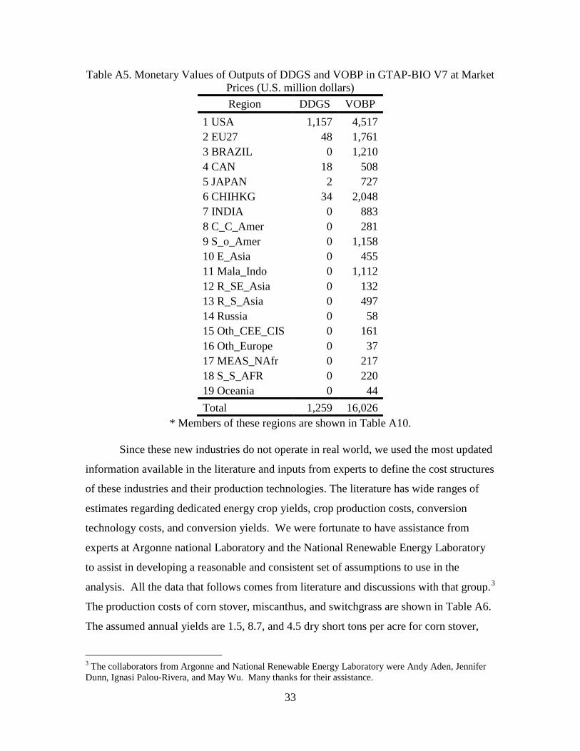
VOBP. Table A5 represent monetary values of DDGS and VOBP at market prices by
region in the new database.
32
Table A4. Monetary Values of Outputs of Crude and Refined Vegetable Oil Industries in GTAP-BIO V7 at Market Prices (U.S. million dollars)
Region Cveg Rveg 1 USA 7,657 8,546 2 EU27 6,989 28,890 3 BRAZIL 5,686 6,094 4 CAN 1,130 2,243 5 JAPAN 1,672 3,931 6 CHIHKG 3,515 3,963 7 INDIA 2,456 5,870 8 C_C_Amer 859 3,397 9 S_o_Amer 5,865 6,792 10 E_Asia 892 1,179 11 Mala_Indo 7,428 11,173 12 R_SE_Asia 801 2,546 13 R_S_Asia 911 2,544 14 Russia 506 1,704 15 Oth_CEE_CIS 1,030 3,740 16 Oth_Europe 147 635 17 MEAS_NAfr 1,016 2,879 18 S_S_AFR 937 2,666 19 Oceania 427 2,109 Total 49,924 100,899
* Members of these regions are shown in Table A10.
5. Introducing Cellulosic Feedstock Industries into the Database
The following feedstock industries are introduced into the database to support
production of advance biofuels:
- Corn stover industry, which collects corn stover from croplands and delivers the
collected corn stover to the cellulosic biofuel industries,
- Miscanthus industry, which produces miscanthus and delivers its output to the
cellulosic biofuel industries,
- Switchgrass industry, which produces switchgrass and delivers its output to the
cellulosic biofuel industries.
33
Table A5. Monetary Values of Outputs of DDGS and VOBP in GTAP-BIO V7 at Market Prices (U.S. million dollars) Region DDGS VOBP
1 USA 1,157 4,517 2 EU27 48 1,761 3 BRAZIL 0 1,210 4 CAN 18 508 5 JAPAN 2 727 6 CHIHKG 34 2,048 7 INDIA 0 883 8 C_C_Amer 0 281 9 S_o_Amer 0 1,158 10 E_Asia 0 455 11 Mala_Indo 0 1,112 12 R_SE_Asia 0 132 13 R_S_Asia 0 497 14 Russia 0 58 15 Oth_CEE_CIS 0 161 16 Oth_Europe 0 37 17 MEAS_NAfr 0 217 18 S_S_AFR 0 220 19 Oceania 0 44 Total 1,259 16,026
* Members of these regions are shown in Table A10.
Since these new industries do not operate in real world, we used the most updated
information available in the literature and inputs from experts to define the cost structures
of these industries and their production technologies. The literature has wide ranges of
estimates regarding dedicated energy crop yields, crop production costs, conversion
technology costs, and conversion yields. We were fortunate to have assistance from
experts at Argonne national Laboratory and the National Renewable Energy Laboratory
to assist in developing a reasonable and consistent set of assumptions to use in the
analysis. All the data that follows comes from literature and discussions with that group.3
The production costs of corn stover, miscanthus, and switchgrass are shown in Table A6.
The assumed annual yields are 1.5, 8.7, and 4.5 dry short tons per acre for corn stover,
3 The collaborators from Argonne and National Renewable Energy Laboratory were Andy Aden, Jennifer Dunn, Ignasi Palou-Rivera, and May Wu. Many thanks for their assistance.

34
miscanthus, and switchgrass, respectively. For corn stover, we assumed that 33 percent
of the available stover could be removed and the rest left on the field to prevent erosion
and loss of soil carbon.
Table A6. Production Costs of Corn Stover, Miscanthus and Switchgrass at 2010 Prices
(U.S. dollars per dry short ton) Cost item Stover Miscanthus Switchgrass Fertilizer 20.34 16.47 16.47 Harvesting costs: 20.19 35.56 35.56 Fuel 3.06 5.39 5.39 Labor 3.31 5.83 5.83 Equipment 7.38 13.00 13.00 Other 6.44 11.34 11.34 Transport: 30.00 30.00 30.00 Labor 15.00 15.00 15.00 Equipment 10.00 10.00 10.00 Fuel 5.00 5.00 5.00 Storage 18.94 13.00 13.00 Seeding 0.00 19.69 4.52 Land rent 0.00 11.31 21.82 Total cost with no rent 89.47 114.71 99.55 Total cost with rent 89.47 126.03 121.37
Source: Authors’ estimates in consultation with Argonne and National Renewable Energy Laboratory.
Then using the U.S. GDP deflator we adjusted these cost items (except for land
rent) to the price level of 2004 to make them consistent with the price level of GTAP
database. For land we followed a different method to adjust its value to 2004. This
method is explained later in this section. According to our calculations, corn stover,
miscanthus, and switchgrass are priced at $78, $103.12, and $92.45 per short ton
respectively at 2004 prices. We converted cost items noted in Table A6 in terms of cost
items in GTAP database. These cost structures are shown in Table A7. This table
indicates that capital is a major cost item in these new industries. This table also shows
that items such as transportation, fertilizer, and labor have significant shares in the cost
structures of these new industries. As shown in Tables A6 and A7, unlike the corn stover
industry, the miscanthus and switchgrass industries use land as an input in the production
process. The costs of land for miscanthus and switchgrass industries are determined

35
based on yield of 8.7 and 4.5 short tons per acre for miscanthus and switchgrass,
respectively. The rent value for land under production of these crops is assumed to be
about $60 per hectare ($24.3 per acre) in 2004. This value is obtained according to the
average of land rents in wheat, coarse grains, oilseeds, and livestock industries in GTAP
2004 database.
To introduce the corn stover, miscanthus, and switchgrass industries into the
database, we assumed that some regions including the U.S., Brazil, China, France,
Germany, and the U.K. produce tiny amounts of these products in 2004 and converts
them to advance biofuels. The SplitCom program was used to introduce these industries
into the new database.
Table A7. Cost Structures of Corn Stover, Miscanthus, and Switchgrass Sctivities
(percentages of total costs) Cost Items Corn Stover Miscanthus Switchgrass
Fertilizer 22.7 14.0 15.6 Transportation 33.5 25.4 28.4 Fuel 3.4 4.6 5.1 Payments to seed company 0.0 6.7 1.7 Other costs 7.0 7.5 8.0 Labor 10.0 10.7 11.5 Land 0.0 2.7 5.8 Capital (including profit) 23.3 28.5 23.9 Total 100.0 100.0 100.0 Source: Authors’ estimates.
6. Introducing Advanced Cellulosic Biofuels into the Database
Six cellulosic biofuel producers which convert cellulosic feedstocks to advanced
biofuels were introduced into the database – three for ethanol and three for bio-gasoline.
In other words, there is a separate industry for each feedstock (stover, miscanthus, and
switchgrass). For bio-gasoline, the industries are identical. For ethanol, the stover
industry is somewhat different from the dedicated energy crop industry as shown in the
base production cost data in Table A8. The conversion yield for bio-gasoline is 60
gallons of bio-gasoline per dry ton (regardless of feedstock). For ethanol, the conversion
yield is 75 gallons of ethanol per dry ton regardless of feedstock. It is also assumed that
the price of the advanced biofuels is equal to their production costs.

36
Table A9 provides the cost structure for the biofuel industries. This table indicates
that capital and feedstock are major cost items for biofuel producers. Even though these
industries may produce by-products (such as electricity and other energy products), their
shares are so small that we ignore here. However, we also assumed that the advanced
biofuel producers will get $1.01subsidy per gallon of produced fuel in the base case. The
SplitCom program was used to introduce these industries into the new GTAP-BIO
database.
Table A8. Biofuel Production Costs
Cost Items FeedStock ($ / dry short ton)
Pathways Thermo - Gasoline
Bio - Ethanol - Stover
Bio - Ethanol - Dedicated Crops
Capital cost ($/gal.) $1.14 $0.51 $0.57 Operating cost ($/gal.) $0.49 $1.34 $1.52 Feedstock cost:
Stover ($/gal) $89.47 $1.49 $1.19 Switchgrass ($/gal) $121.37 $2.02 $1.62 Miscanthus ($/gal) $126.03 $2.10 $1.68
Total cost - stover $3.12 $3.05 Total cost - switchgrass $3.65 $3.71 Total cost - miscanthus $3.73 $3.77
Source: Authors’ estimates in consultation with Argonne and National Renewable Energy Laboratory.
Table A9. Cost Structures of Advanced Biofuel Producers (percentage of total costs)
Cost items Bio-gasoline Ethanol
Miscanthus Switchgrass Corn stover Miscanthus Switchgrass Corn
stover Feedstock 54.6 51.9 47.7 42.9 40.2 39.2 Chemicals 0.0 0.0 0.0 15.6 16.3 18.8 Energy 1.0 1.0 1.1 4.1 4.2 4.9 Other costs 10.5 11.1 12.1 17.5 18.3 15.0 Labor 2.2 2.4 2.6 4.4 4.6 5.3 Capital 31.8 33.7 36.6 15.6 16.3 16.9 Total 100.0 100.0 100.0 100.0 100.0 100.0 Source: [24, 25]

37
7. Other Modifications and Components
To support and facilitate research on the economic and environmental
consequences of international biofuel programs we added several headers to the
GTAP_BIOB_ADF_V7 database. These headers include land use and land cover by
country and AEZ in 2004, land rents by country and AEZ in 2004, global liquid biofuel
consumption in 2004, emissions data due to production and consumption of all types of
energy commodities, and crop production and harvested areas in 2004 by country and
AEZ.
8. Aggregation Scheme Used in This Paper
Table A10. Regions and Their Members
Region Description Corresponding Countries in GTAP
USA United States Usa
EU27 European Union 27 aut, bel, bgr, cyp, cze, deu, dnk, esp, est, fin, fra, gbr, grc, hun, irl, ita, ltu, lux, lva, mlt, nld, pol, prt, rom, svk, svn, swe
BRAZIL Brazil Bra
CAN Canada Can
JAPAN Japan Jpn
CHIHKG China and Hong Kong chn, hkg
INDIA India Ind
C_C_Amer Central and Caribbean Americas mex, xna, xca, xfa, xcb
S_o_Amer South and Other Americas col, per, ven, xap, arg, chl, ury, xsm
E_Asia East Asia kor, twn, xea
Mala_Indo Malaysia and Indonesia ind, mys
R_SE_Asia Rest of South East Asia phl, sgp, tha, vnm, xse
R_S_Asia Rest of South Asia bgd, lka, xsa
Russia Russia Rus
Oth_CEE_CIS Other East Europe and Rest of Former Soviet Union xer, alb, hrv, xsu, tur
R_Europe Rest of European Countries che, xef
MEAS_NAfr Middle Eastern and North Africa xme,mar, tun, xnf
S_S_AFR Sub Saharan Africa Bwa, zaf, xsc, mwi, moz, tza, zmb, zwe, xsd, mdg, uga, xss
Oceania Oceania countries aus, nzl, xoc

38
Table A11. List of Industries and Commodities in the New Model Industry Commodity Description Name in the GTAP_BIOB Paddy_Rice Paddy_Rice Paddy rice Pdr Wheat Wheat Wheat Wht CrGrains CrGrains Cereal grains Gro Oilseeds Oilseeds Oil seeds Osd OthAgri OthAgri Other agriculture goods ocr, pfb, v_f Sugarcane Sugarcane Sugar cane and sugar beet c-b Miscanthus Miscanthus A dedicated crop to be used in biofuel New Switchgrass Switchgrass A dedicated crop to be used in biofuel New Stover Stover Collected corn stover to be used in biofuel New DairyFarms DairyFarms Dairy Products Rmk Ruminant Ruminant Cattle & ruminant meat production and Ctl, wol NonRum Non-Rum Non-ruminant meat production oapl ProcDairy ProcDairy Processed dairy products Mil ProcRum ProcRum Processed ruminant meat production Cmt ProcNonRum ProcNonRum Processed non-ruminant meat production Omt Forestry Forestry Forestry Frs
Cveg_Oil Cveg_Oil Crude vegetable oil A portion of vol VOBP Oil meals A portion of vol
Rveg_Oil Rveg_Oil Refined vegetable oil A portion of vol Proc_Rice Proc_Rice Processed rice Pcr Bev_Sug Bev_Sug Beverages, tobacco, and sugar b_t, sgr Proc_Food Proc_Food Processed food products A portion of ofd Proc_Feed Proc_Feed Processed animal feed products A portion of ofd OthPrimSect OthPrimSect Other Primary products fsh, omn Coal Coal Coal Coa Oil Oil Crude Oil Oil Gas Gas Natural gas gas, gdt Oil_Pcts Oil_Pcts Petroleum and coal products p-c Electricity Electricity Electricity Ely En_Int_Ind En_Int_Ind Energy intensive Industries crpn, i_s, nfm, fmp
Oth_Ind_Se Oth_Ind_Se Other industry and services atp, cmn, cns, ele, isr, lea, lum, mvh, nmm, obs, ofi, ome, omf, otn, otp, ppp, ros, tex, trd, wap, wtp
NTrdServices BTrdServices Services generating Non-C02 Emissions wtr, osg, dwe AdvfB-Misc AdvfB-Misc Bio-Gasoline produced from miscanthus New AdvfB-Swit AdvfB-Swit Bio-Gasoline produced from switchgrass New AdvfB-Stover AdvfB-Stover Bio-Gasoline produced from corn stover New AdvfE-Misc AdvfE-Misc Ethanol produced from miscanthus New AdvfE-Swit AdvfE-Swit Ethanol produced from switchgrass New AdvfE-Stover AdvfE-Stover Ethanol produced from corn stover New
EthanolC Ethanol1 Ethanol produced from grains New DDGS Dried Distillers Grains with Solubles New
Ethanol2 Ethanol2 Ethanol produced from sugarcane New Biodiesel Biodiesel Biodiesel produced from vegetable oil New

39
Appendix B
Introducing Advanced Biofuels into the GTAP Modeling Framework
1. Modifications in GTAP Modeling Structure
1.1. Demand Side Modifications
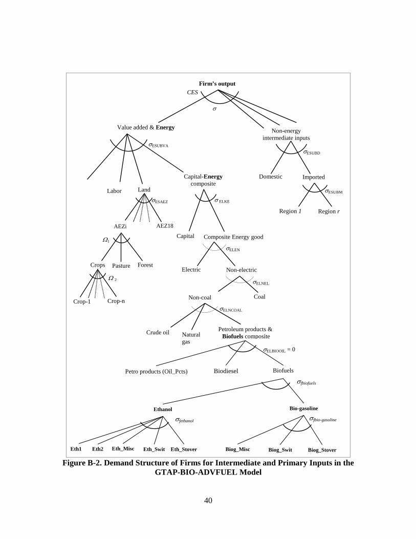
On the demand side, we introduced bio-gasoline and ethanol from miscanthus,
switchgrass, and corn stover in the demand structure of households and firms as a
substitute for fossil fuels and biofuels. Figures B-1 and B-2 represent these demands.
Figure B-1. Household Demand Structure in the GTAP-BIO-ADVFUEL Model
Household Demand for Private Goods
Energy Composite
CDE
Non-Energy Commodities
Coal Petroleum products & Biofuels composite
σELEGY
Petro products (Oil_Pcts)
σELHBIOIL
Biofuels
Oil Gas Electricity
CES
Ethanol
Eth1
BBiiooddiieesseell
Bio-gasoline
σbiofuels
Eth2 Eth_Misc Eth_Swit Eth_Stover Biog_Misc Biog_Swit Biog_Stover
σethanol σbio-gasoline
40
Figure B-2. Demand Structure of Firms for Intermediate and Primary Inputs in the GTAP-BIO-ADVFUEL Model
Firm’s output
Imported
Region r
Value added & Energy Non-energy intermediate inputs
σ
σESUBD
Capital-Energy composite
σESUBVA
Land Labor
Region 1
Domestic
σESUBM
σ ELKE
Non-electric
Capital
Electric
Coal
σELNEL
Petroleum products & Biofuels composite
Crude oil
σELNCOAL
Non-coal
Petro products (Oil_Pcts)
σELBIOOIL = 0
Biofuels
Composite Energy good
σELEN
Natural gas
AEZi AEZ18
σESAEZ
CES
Ω1
Crops Pasture Forest
Crop-1 Crop-n
Ω 2
Biodiesel
Ethanol
Eth1
Bio-gasoline
Eth2 Eth_Misc Eth_Swit Eth_Stover Biog_Misc Biog_Swit Biog_Stover
σfbio-gasoline σfethanol
σfbiofuels

41
1.2. Modifications in the Land Market
In our earlier work the land supply module consisted of a two-level nesting
structure. In this nesting format the lowest level allocates land supply among three land
cover categories of forest, pasture, and cropland, and the upper level allocates croplands
among crop activities including CRP and cropland-pastures. In the two-level nesting
structure only one parameter (ETL2) governs allocation of cropland supply among all
types of crops. In this work we extended the land supply structure to three levels. The
lowest level of the new land supply model is the same as what we had before. The second
level divides cropland supply into two main crop categories. The first group covers all
traditional crops including rice, wheat, coarse grains, oilseeds, vegetable and fruits, sugar
crops, other crops, and CRP land. The second group covers dedicated energy crops and
cropland-pasture. The top level of this three-level nesting structure determines supply of
cropland to each crop industry. This nesting structure allows us to assign different land
transformation elasticities among the first and second groups of crops.
Figure B-3 of this appendix represents the new and old land supply structure. We
made this change because it more closely represents the agronomic and economic reality.
Dedicated energy crops such as miscanthus and switchgrass are much more likely to
compete with cropland pasture than they are to compete with much more productive
cropland used for corn, soybeans, etc. Thus, the new structure better reflects what would
likely emerge in this new production activity. As shown in Figure B-3 in the new model,
miscanthus competes with cropland pasture which is an input for the livestock industry.
Figure B-3 represents competition in the land market between different agricultural
activities in the model. Compared to the earlier model the new land supply structure
provides more flexibility in the land market to satisfy the higher demand for miscanthus
and switchgrass to meet the production targets for cellulosic biofuels. In addition, for the
new model we assigned a larger elasticity of transformation to the crop nests to facilitate
conversion of one type of cropland to other types as discussed in the text. In the new
land supply structure we applied the following land transformation elasticities:
- Transformation elasticity among forest, pastureland, and cropland = - 0.2 (no change)
- Transformation elasticity among the first and second groups of crops = - 0.75,

42
- Transformation elasticity among traditional crops = - 0.75
- Transformation elasticity among cropland pasture, miscanthus, and switchgrass = - 10
Figure B-3. Land Cover and Land Use Activities in the Old and New GTAP-BIO-
ADV
Land Supply
CRP Crop 1 Crop n
Forest Pasture Cropland
Cropland-Pasture
Old Model
Land Supply
Pasture Forest
Crop N Miscanthus Switchgrass
Crop group 2
Cropland
CRP
Crop group 1
Crop 1
New Model
Cropland-Pasture
Ω1
Ω2
Ω4 Ω5

43
1.3. Other Modifications
We revised all necessary GTAP codes and files to support the new model. That
includes revising the main GTAP Table file, GTAP parameter file, and the GTAP set
files.
44
Appendix C Experiments Used in This Study
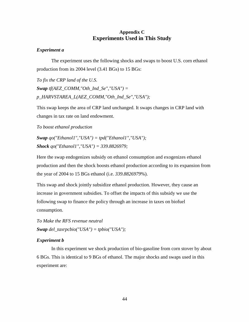
Experiment a
The experiment uses the following shocks and swaps to boost U.S. corn ethanol
production from its 2004 level (3.41 BGs) to 15 BGs:
To fix the CRP land of the U.S.
Swap tf(AEZ_COMM,"Oth_Ind_Se","USA") =
p_HARVSTAREA_L(AEZ_COMM,"Oth_Ind_Se","USA");
This swap keeps the area of CRP land unchanged. It swaps changes in CRP land with
changes in tax rate on land endowment.
To boost ethanol production
Swap qo("Ethanol1","USA") = tpd("Ethanol1","USA");
Shock qo("Ethanol1","USA") = 339.8826979;
Here the swap endogenizes subsidy on ethanol consumption and exogenizes ethanol
production and then the shock boosts ethanol production according to its expansion from
the year of 2004 to 15 BGs ethanol (i.e. 339.8826979%).
This swap and shock jointly subsidize ethanol production. However, they cause an
increase in government subsidies. To offset the impacts of this subsidy we use the
following swap to finance the policy through an increase in taxes on biofuel
consumption.
To Make the RFS revenue neutral
Swap del_taxrpcbio("USA") = tpbio("USA");
Experiment b
In this experiment we shock production of bio-gasoline from corn stover by about
6 BGs. This is identical to 9 BGs of ethanol. The major shocks and swaps used in this
experiment are:

45
To fix the CRP land of the U.S.
Swap tf(AEZ_COMM,"Oth_Ind_Se","USA") =
p_HARVSTAREA_L(AEZ_COMM,"Oth_Ind_Se","USA");
To boost bio-gasoline production from corn stover
Swap qo("adv_Stover","USA") = tpd("advf_Stover","USA");
Shock qo("advf_Stover","USA") = 777484.822;
To Make the RFS revenue neutral
Swap del_taxrpcbio("USA") = tpbio("USA");
Experiment c
In this experiment we shock production of bio-gasoline from miscanthus by about
4.7 BGs. This is identical to 7.0 BGs of ethanol. The major shocks and swaps used in this
experiment are:
To fix the CRP land of the U.S.
Swap tf(AEZ_COMM,"Oth_Ind_Se","USA") =
p_HARVSTAREA_L(AEZ_COMM,"Oth_Ind_Se","USA");
To boost bio-gasoline production from corn stover
Swap qo("adv_Misc","USA") = tpd("advf_Misc","USA");
Shock qo("advf_Misc","USA") = 609008.110;
To Make the RFS revenue neutral
Swap del_taxrpcbio("USA") = tpbio("USA"
Experiment d
In this experiment we shock production of bio-gasoline from switchgrass by about
4.7 BGs. This is identical to 7.0 BGs of ethanol. The major shocks and swaps used in this
experiment are:
To fix the CRP land of the U.S.
Swap tf(AEZ_COMM,"Oth_Ind_Se","USA") =
p_HARVSTAREA_L(AEZ_COMM,"Oth_Ind_Se","USA");
46
To boost bio-gasoline production from switchgrass
Swap qo("advfB_Swit","USA") = tpd("advBf_Swit","USA");
Shock qo("advfB_Swit","USA") = 710513.849;
To Make the RFS revenue neutral
Swap del_taxrpcbio("USA") = tpbio("USA");
Experiment e
In this experiment we shock production of ethanol from corn stover by about 9
BGs. The major shocks and swaps used in this experiment are:
To fix the CRP land of the U.S.
Swap tf(AEZ_COMM,"Oth_Ind_Se","USA") =
p_HARVSTAREA_L(AEZ_COMM,"Oth_Ind_Se","USA");
To boost bio-gasoline production from corn stover
Swap qo("advfB_Stover","USA") = tpd("advfB_Stover","USA");
Shock qo("advfB_Stover","USA") = 1088565.780;
To Make the RFS revenue neutral
Swap del_taxrpcbio("USA") = tpbio("USA");
To adjust the energy content of ethanol to gasoline
shock afenergy("AdvfE_Stover", "USA")=-33;
shock ahenergy("AdvfE_Stover", "USA")=-33;
Experiment f
In this experiment we shock production of ethanol from miscanthus by about 7
BGs. The major shocks and swaps used in this experiment are:
To fix the CRP land of the U.S.
Swap tf(AEZ_COMM,"Oth_Ind_Se","USA") =
p_HARVSTAREA_L(AEZ_COMM,"Oth_Ind_Se","USA");
To boost bio-gasoline production from miscanthus

47
Swap qo("advfE_Misc","USA") = tpd("advfE_Misc","USA");
Shock qo("advfE_Misc","USA") = 846640.051;
To adjust the energy content of ethanol to gasoline
shock afenergy("AdvfE_Misc", "USA")=-33;
shock ahenergy("AdvfE_Misc", "USA")=-33;
To Make the RFS revenue neutral
Swap del_taxrpcbio("USA") = tpbio("USA");
Experiment g
In this experiment we shock production of ethanol from switchgrass by about 7
BGs. The major shocks and swaps used in this experiment are:
To fix the CRP land of the U.S.
Swap tf(AEZ_COMM,"Oth_Ind_Se","USA") =
p_HARVSTAREA_L(AEZ_COMM,"Oth_Ind_Se","USA");
To boost ethanol production from switchgrass
Swap qo("advfE_Swit","USA") = tpd("advfE_Swit","USA");
Shock qo("advfE_Swit","USA") = 846640.051;
To adjust the energy content of ethanol to gasoline
shock afenergy("AdvfE_Swit", "USA")=-33;
shock ahenergy("AdvfE_Swit", "USA")=-33;
To Make the RFS revenue neutral
Swap del_taxrpcbio("USA") = tpbio("USA");
Related Documents


![United States Court of Appeals...generating [cellulosic-biofuel] RINs.” 40 C.F.R. § 80.1450(b)(1)(xiii)(B)(2). To enable EPA to determine whether a producer’s cellulosic converted](https://static.cupdf.com/doc/110x72/60bc1b46118e541c600a4e4c/united-states-court-of-appeals-generating-cellulosic-biofuel-rinsa-40-cfr.jpg)
