NBER WORKING PAPER SERIES GLOBAL FIRMS Andrew B. Bernard J. Bradford Jensen Stephen J. Redding Peter K. Schott Working Paper 22727 http://www.nber.org/papers/w22727 NATIONAL BUREAU OF ECONOMIC RESEARCH 1050 Massachusetts Avenue Cambridge, MA 02138 October 2016 This paper was commissioned for the Journal of Economic Literature. We are grateful to Janet Currie and Steven Durlauf for their encouragement. We would like to thank Steven Durlauf, six referees, Pol Antras, Joaquin Blaum, Peter Neary, David Weinstein and conference and seminar participants at CEPR, NOITS, Oxford and UIBE for helpful comments. Bernard, Jensen, Redding and Schott thank Tuck, Georgetown, Princeton and Yale respectively for research support. We thank Jim Davis from Census for handling disclosure. The empirical research in this paper was conducted at the Boston, New York and Washington U.S. Census Regional Data Centers. Any opinions, findings, and conclusions or recommendations expressed in this material are those of the authors and do not necessarily reflect the views of the U.S. Census Bureau, the National Bureau of Economic Research, the Centre for Economic Policy Research, the National Bureau of Economic Research, or any other institution to which the authors are affiliated. Results have been screened to ensure that no confidential data are revealed. NBER working papers are circulated for discussion and comment purposes. They have not been peer-reviewed or been subject to the review by the NBER Board of Directors that accompanies official NBER publications. © 2016 by Andrew B. Bernard, J. Bradford Jensen, Stephen J. Redding, and Peter K. Schott. All rights reserved. Short sections of text, not to exceed two paragraphs, may be quoted without explicit permission provided that full credit, including © notice, is given to the source.

Welcome message from author
This document is posted to help you gain knowledge. Please leave a comment to let me know what you think about it! Share it to your friends and learn new things together.
Transcript

NBER WORKING PAPER SERIES
GLOBAL FIRMS
Andrew B. BernardJ. Bradford JensenStephen J. Redding
Peter K. Schott
Working Paper 22727http://www.nber.org/papers/w22727
NATIONAL BUREAU OF ECONOMIC RESEARCH1050 Massachusetts Avenue
Cambridge, MA 02138October 2016
This paper was commissioned for the Journal of Economic Literature. We are grateful to Janet Currie and Steven Durlauf for their encouragement. We would like to thank Steven Durlauf, six referees, Pol Antras, Joaquin Blaum, Peter Neary, David Weinstein and conference and seminar participants at CEPR, NOITS, Oxford and UIBE for helpful comments. Bernard, Jensen, Redding and Schott thank Tuck, Georgetown, Princeton and Yale respectively for research support. We thank Jim Davis from Census for handling disclosure. The empirical research in this paper was conducted at the Boston, New York and Washington U.S. Census Regional Data Centers. Any opinions, findings, and conclusions or recommendations expressed in this material are those of the authors and do not necessarily reflect the views of the U.S. Census Bureau, the National Bureau of Economic Research, the Centre for Economic Policy Research, the National Bureau of Economic Research, or any other institution to which the authors are affiliated. Results have been screened to ensure that no confidential data are revealed.
NBER working papers are circulated for discussion and comment purposes. They have not been peer-reviewed or been subject to the review by the NBER Board of Directors that accompanies official NBER publications.
© 2016 by Andrew B. Bernard, J. Bradford Jensen, Stephen J. Redding, and Peter K. Schott. All rights reserved. Short sections of text, not to exceed two paragraphs, may be quoted without explicit permission provided that full credit, including © notice, is given to the source.

Global FirmsAndrew B. Bernard, J. Bradford Jensen, Stephen J. Redding, and Peter K. SchottNBER Working Paper No. 22727October 2016JEL No. F12,F14,L11,L21
ABSTRACT
Research in international trade has changed dramatically over the last twenty years, as attention has shifted from countries and industries towards the firms actually engaged in international trade. The now-standard heterogeneous firm model posits measure zero firms that compete under monopolistic competition and decide whether to export to foreign markets. However, much of international trade is dominated by a few “global firms,” which participate in the international economy along multiple margins and account for substantial shares of aggregate trade. We develop a new theoretical framework that allows firms to have large market shares and to decide simultaneously on the set of production locations, export markets, input sources, products to export, and inputs to import. Using U.S. firm and trade transactions data, we provide strong evidence in support of this framework's main predictions of interdependencies and complementarities between these margins of firm international participation. Global firms participate more intensively along each margin, magnifying the impact of underlying differences in firm characteristics, and increasing their shares of aggregate trade.
Andrew B. BernardTuck School of Business at Dartmouth100 Tuck HallHanover, NH 03755and CEPRand also [email protected]
Stephen J. ReddingDepartment of Economicsand Woodrow Wilson SchoolPrinceton UniversityFisher HallPrinceton, NJ 08544and [email protected]
J. Bradford JensenMcDonough School of BusinessGeorgetown UniversityWashington, DC 20057and Peterson Institute for International Economics and also [email protected]
Peter K. SchottYale School of Management 135 Prospect StreetNew Haven, CT 06520-8200 and [email protected]

Global Firms
1 Introduction
Research in international trade has changed dramatically over the last twenty years, as attention has shifted
from countries and industries towards rms. An initial wave of empirical research established a series
of stylized facts: only some rms export, exporters are more productive than non-exporters, and trade
liberalization is accompanied by an increase in aggregate industry productivity. Subsequent theoretical
research emphasized reallocations of resources within and across rms as well as endogenous changes
in rm productivity in a setting in which measure zero rms compete under monopolistic competition
and self-select into export markets (e.g., Melitz (2003)). This new theoretical research generated additional
empirical predictions, which in turn led to a further wave of empirical research and an ongoing dialogue
between theory and evidence.1
In this paper, we argue that this standard paradigm does not go far enough in recognizing the role
of “global rms,” which we dene as rms that participate in the international economy along multiple
margins and account for substantial shares of aggregate trade. We develop a new theoretical framework
that incorporates a wider range of margins of participation in the international economy than previous
research. Each rm can choose production locations in which to operate plants; export markets for each
plant; products to export from each plant to each market; exports of each product from each plant to
each market; the countries from which to source intermediate inputs for each plant; and imports of each
intermediate input from each source country by each plant. Firms that participate so extensively in the
international economy are unlikely to be measure zero and indeed account for substantial shares of ob-
served trade. Therefore we allow these global rms to internalize the eects of their pricing and product
introduction decisions on market aggregates. Despite allowing for such eects on market aggregates and
incorporating a rich range of rm decision margins, our model remains tractable and amenable to em-
pirical analysis. The key contribution of this review relative to our previous surveys (cited in footnote 1)
is that we use this new theoretical framework to derive four sets of key predictions on which we present
empirical evidence. Some of this evidence updates previous ndings for earlier years, in which case we use
our framework to draw out new insights and highlight changes over time. Other evidence is distinctive to
this review and relates directly to the predictions of our new theoretical framework.
Our empirical work is organized around the following four sets of theoretical predictions. First, rm
decisions for each margin of participation in the international economy are interdependent. For example,
importing decisions are interdependent across countries, because the decision to incur the xed costs
of sourcing inputs from one country gives the rm access to lower-cost suppliers, which reduces rm
production costs and prices. These lower prices in turn imply a larger scale of operation, which makes
it more likely that the rm will nd it protable to incur the xed costs of sourcing inputs from other
1For earlier surveys of this theoretical and empirical literature, see Bernard, Jensen, Redding, and Schott (2007), Bernard,
Jensen, Redding, and Schott (2012), Melitz and Treer (2015), Melitz and Redding (2014a) and Redding (2011). For broader surveys
of rm organization and trade, see Antràs (2015), Antràs and Rossi-Hansberg (2009) and Helpman (2006).
1

Global Firms
countries (as in Tintelnot (2016) and Antràs, Fort, and Tintelnot (2014)). Exporting and importing decisions
are also interdependent with one another, because incurring the xed exporting cost for an additional
market increases rm revenue, which makes it more likely that the rm will nd it protable to incur the
xed cost of sourcing inputs from any given country. This interaction between exporting and importing
in turn implies that exporting decisions are interdependent across countries. Incurring the xed exporting
cost for an additional market increases rm revenue, which makes it more likely that the rm will nd it
protable to incur the xed cost of importing inputs from another country. This in turn reduces variable
production costs and prices, and thereby increases revenue. which makes it more likely that the rm will
nd it protable to incur the xed exporting cost for another market. More generally, the choices of the
set of markets to serve, the set of products to export, and the set of countries from which to source inputs
(the “extensive margins”) aect variable production costs and prices, which implies that they inuence
exports of each product to each market and imports of each input from each source country (the “intensive
margins”). In a world of such interdependent rm decisions, understanding the eects of a reduction in
trade costs on any one margin (e.g. exports of a given product to a given country) requires taking into
account its eects on all other margins (through the organization of global production chains that involve
imports as well as exports).
Second, rm decisions along multiple margins of international participation magnify the eects of
dierences in exogenous primitives (e.g. exogenous components of rm productivity) on endogenous
outcomes (e.g. rm sales and employment). More productive rms participate more intensively in the
world economy along each margin. Therefore small dierences in rm productivity can have magnied
consequences for rm sales and employment, as more productive rms lower their production costs by
sourcing inputs from more countries, and also expand their scale of operation by exporting more products
to each market and exporting to more markets. Similarly, small changes in exogenous trade costs can have
magnied eects on endogenous trade ows, as they induce rms to serve more markets, export more
products to each market, export more of each product, source intermediate inputs from more countries,
and import more of each intermediate input from each source country.
Third, rms that participate so intensively in the international economy are unlikely to be measure
zero, and hence their choices can aect market aggregates, which gives rise to strategic market power.
Firms with larger market shares have greater eects on market aggregates, and hence they face lower
perceived elasticities of demand, which implies that they charge lower markups of price over marginal
cost. This mechanism for variable markups operates across a range of dierent functional forms for de-
mand, including constant elasticity of substitution (CES) preferences. These variable markups provide a
natural explanation for empirical ndings of “pricing to market,” where rms charge dierent prices in
dierent markets. Such price dierences arise because rm markups vary endogenously across markets,
depending on rm sales shares within each market. Variable markups provide a natural rationalization
for empirical evidence of “incomplete pass-through,” whereby cost shocks are not passed through fully
2

Global Firms
into consumer prices. The reason is that as cost shocks are transmitted to prices, they result in endoge-
nous adjustments in sales shares, which lead to osetting changes in rm markups. In addition to this
strategic market power, when rms participate in international markets by exporting multiple products,
they internalize the cannibalization eects from the introduction of new products on the sales of existing
products. Hence multi-product rms make systematically dierent product introduction decisions from
single-product rms.
Fourth, the magnication of exogenous dierences across rms through multiple, interdependent and
complementary margins of international participation implies that aggregate trade is concentrated in the
hands of a relatively small number of rms. Therefore our framework oers new insights for under-
standing the skewed distribution of sales across rms that has been the subject of much attention in the
industrial organization literature (e.g. Sutton (1997) and Axtell (2001)). To infer the underlying distribution
of rm productivity from the observed distribution of rm sales requires taking into account the multiple,
interdependent and complementary rm decisions (such as to enter export markets, supply products and
source intermediate inputs) that aect rm sales.
Our paper is related to the inuential line of research that has modeled rm heterogeneity in dierenti-
ated product markets following Melitz (2003).2
In this model, a competitive fringe of potential rms decide
whether to enter an industry by paying a xed entry cost which is thereafter sunk. Potential entrants face
ex ante uncertainty concerning their productivity. Once the sunk entry cost is paid, a rm draws its pro-
ductivity from a xed distribution and productivity remains xed thereafter. Firms produce horizontally
dierentiated varieties within the industry under conditions of monopolistic competition.3
The existence
of xed production costs implies that a rm drawing a productivity below the “zero-prot productivity
cuto” would make negative prots from producing and hence chooses instead to exit the industry. Fixed
and variable costs of exporting ensure that only those active rms that draw a productivity above a higher
“export productivity cuto” nd it protable to export.4
Following multilateral trade liberalization, high-
productivity exporting rms experience increased revenue through greater export market sales; the most
productive non-exporters now nd it protable to enter export markets, increasing the fraction of export-
ing rms; the least productive rms exit; and there is a contraction in the revenue of surviving rms that
only serve the domestic market. Each of these responses reallocates resources towards high-productivity
rms and raises aggregate productivity through a change in industry composition.5
Our contribution relative to this theoretical research is to develop a framework that incorporates a
2See also Bernard, Redding, and Schott (2007) and Melitz and Ottaviano (2008).
3For alternative approaches to rm heterogeneity, see Bernard, Eaton, Jensen, and Kortum (2003) and Yeaple (2005).
4While the original model focuses on exporting, this framework is extended to incorporate foreign direct investment (FDI) as
an alternative mode for servicing foreign markets in Helpman, Melitz, and Yeaple (2004).
5While rm productivity is xed in the Melitz (2003) model, subsequent research has incorporated endogenous decisions that
aect rm productivity through a variety of mechanisms, including technology adoption (Constantini and Melitz (2008), Bustos
(2011) and Lileeva and Treer (2010)), innovation (Atkeson and Burstein (2010), Perla, Tonetti, and Waugh (2015) and Sampson
(2015)), endogenous changes in workforce composition (Helpman, Itskhoki, and Redding (2010) and Helpman, Itskhoki, Muendler,
and Redding (2016)) and endogenous changes in product mix (Bernard, Redding, and Schott (2010, 2011)).
3

Global Firms
wider range of rm margins of international participation than in prior research. Each rm chooses the
set of export market to serve (as in Eaton, Kortum, and Kramarz (2011)) and the set of products to supply to
each export market (as in Bernard, Redding, and Schott (2010, 2011) and Hottman, Redding, and Weinstein
(2016)).6
Each rm also chooses the set of countries from which to source intermediate inputs and which
inputs to import from each source country (as in Antràs, Fort, and Tintelnot (2014) and Bernard, Moxnes,
and Saito (2014)).7
We provide the rst framework that simultaneously encompasses all of these margins
of international participation and we show how this framework can be used to make sense of a number
of features of U.S. rm and trade transactions data. As rms that participate in the international economy
along all of these margins can account for large shares of sales in individual markets, we allow rms
to internalize their eects on market aggregates then choosing prices, as in Atkeson and Burstein (2008),
Eaton, Kortum, and Sotelo (2012), Edmond, Midrigan, and Xu (2012), Gaubert and Itskhoki (2015), Hottman,
Redding, and Weinstein (2016), and Sutton and Treer (2016).8
Our research is also related to the large empirical literature that has examined the relationship between
rm performance and participation in international markets following Bernard and Jensen (1995). Early
empirical studies in this literature used rm and plant-level data to document a number of stylized facts
about exporters and non-exporters. In particular, exporters are larger, more productive, more capital-
intensive, more skill-intensive and pay higher wages than non-exporters within the same industry (see
Bernard and Jensen (1995, 1999)). Subsequent empirical research has used international trade transactions
data to establish additional regularities about rm trade participation following Bernard, Jensen, and Schott
(2009). Much of the variation in aggregate bilateral trade ows is accounted for by the extensive margins
of the number of exporting rms (see Eaton, Kortum, and Kramarz (2004)) and the number of rm-product
observations with positive trade (see Bernard, Jensen, Redding, and Schott (2009)). While the extensive
margins of export rms and products are sharply decreasing in proxies for bilateral trade costs such as
distance, the intensive margin of average exports per rm-product observation with positive trade exhibits
little relationship with these proxies because of changes in export composition (see Bernard, Redding,
and Schott (2011)). We show how our theoretical framework accounts for these properties of rm export
behavior and for a broader range of features of rm participation in the global economy.
Within this empirical literature on export participation, our paper is related to several studies that have
focused on the largest rms in the international economy. Bernard, Jensen, and Schott (2009) documents
the concentration of activity in the largest exporting and importing rms for the U.S. and argues that the
6.Other research on multi-product rms and trade includes Arkolakis, Muendler, and Ganapati (2014), Dhingra (2013), Eckel
and Neary (2010), Feenstra and Ma (2008), Mayer, Melitz, and Ottaviano (2013) and Nocke and Yeaple (2014).
7Firm importing is also examined in Amiti and Konings (2007), Amiti and Davis (2011), Blaum, Lelarge, and Peters (2013,
2014), Goldberg, Khandelwal, Pavcnik, and Topalova (2010), De Loecker, Goldberg, Khandelwal, and Pavcnik (2015) and Halpern,
Koren, and Szeidl (2015).
8A related body of research examines the idea that rms can be “granular,” in the sense that idiosyncratic shocks to individual
rms can inuence aggregate business cycle uctuations, as in Gabaix (2011) and di Giovanni, Levchenko, and Mejean (2014).
For broader arguments for incorporating oligopolistic competition into international trade, see Neary (2003, 2016) and Thisse and
Shimomura (2012).
4

Global Firms
“most globally engaged” rms are more likely to trade with dicult markets and perform foreign direct
investment. Mayer and Ottaviano (2007) establishes a set of regularities for European rms and nds that
the export distribution is highly skewed. Freund and Pierola (2015) examines “export superstars” and nds
that very large rms shape country export patterns. Among 32 countries, the top rm on average accounts
for 14% of a country’s total (non-oil) exports; the top ve rms make up 30%; and the revealed comparative
advantage of countries can be created by a single rm.
Although our theoretical framework incorporates a wider range of margins of international partici-
pation than in previous research, it is necessarily an abstraction and cannot capture all features of rms’
business strategies. In particular, we do not model the formation of individual trading relationships be-
tween buyers and sellers, as in the recent literature on networks in international trade, including Bernard,
Moxnes, and Saito (2014), Bernard, Moxnes, and Ulltveit-Moe (2015), Chaney (2014, 2015), Eaton, Kortum,
Kramarz, and Sampognaro (2014), Eaton, Jinkins, Tybout, and Xu (2016) and Lim (2016). We also abstract
from “carry along trade,” in which a rm exports products that it does not produce, as examined in Bernard,
Blanchard, Beveren, and Vandenbusshe (2015). Our theoretical framework incorporates multinational ac-
tivity to rationalize the trade between related parties that we observe in the U.S. trade transactions data.
Our paper is therefore related to the large literature on multinational rms, including Arkolakis, Ramondo,
Rodriguez-Clare, and Yeaple (2015), Becker and Muendler (2010), Cravino and Levchenko (2015), Hanson,
Mataloni, and Slaughter (2005), Helpman, Melitz, and Yeaple (2004), Ramondo and Rodriguez-Clare (2013),
as reviewed in Antràs and Yeaple (2009). However, as discussed further below, a caveat is that we do not
have data on the overseas production activity of multinational rms, and we only observe related-party
trade when one party to the transaction is located in the United States.
The remainder of the paper is structured as follows. Section 2 develops our theoretical framework. Sec-
tion 3 introduces the data. Section 4 provides empirical evidence on the key predictions of our theoretical
framework. Section 5 concludes.
2 Theoretical Framework
We consider a world of many (potentially) asymmetric countries. Firms are heterogeneous in productiv-
ity and make three sets of decisions: which markets to serve (typically indexed by m), which countries
in produce in (usually denoted by i), and which countries to source inputs from (generally indicated by
j). For each destination market, rms choose the range of products to supply to that market (ordinarily
referenced by k). For each source country, rms choose the range of intermediate inputs to obtain from
that source (most often represented by `). We assume that consumer preferences exhibit a constant elas-
ticity of substitution (CES). However, we allow rms to be large relative to the markets in which they sell
their products, which introduces variable markups (because each rm internalizes the eect of its pricing
choices on market aggregates). We use the rm’s prot maximization problem to derive general proper-
ties of a rm’s decisions to participate in international markets as a function of its productivity that hold
5

Global Firms
regardless of the way in which the model is closed in general equilibrium.
2.1 Preferences
We consider a nested structure of demand as in Hottman, Redding, and Weinstein (2016). Preferences in
each market m are a Cobb-Douglas aggregate of the consumption indices (CGmg) of a continuum of sectors
indexed by g:
ln Um =∫
g∈ΩGλG
mg ln CGmgdg,
∫g∈ΩG
λGmgdg = 1, (1)
where λGmg determines the share of market m’s expenditure on sector g; and ΩG
is the set of sectors.9
The
consumption index (CGmg) for each sector g in each market m is dened over consumption indices (CF
mi f )
for each nal good rm f from each production country i:
CGmg =
∑i∈ΩN
∑f∈ΩF
mig
(λF
mi fCF
mi f
) σFg −1
σFg
σF
gσF
g −1
, σFg > 1, λF
mi f > 0, (2)
where σFg is the elasticity of substitution across rms for sector g; ΩN
is the set of countries; λFmi f is
a demand shifter (“rm appeal”) that captures the overall appeal of the consumption index supplied by
rm f to market m from production country i; and ΩFmig is the set of rms that supply market m from
production country i within sector g.10
The consumption index (CFmi f ) for each rm f from production
location i in market m within sector g is dened over the consumption (CKmik) of each nal product k:
CFmi f =
∑k∈ΩK
mi f
(λK
mikCKmik
) σKg −1
σKg
σK
gσK
g −1
, σKg > 1, λK
mik > 0, (3)
where σKg is the elasticity of substitution across products within rms; λK
mik is a demand shifter (“product
appeal”) that captures the appeal of product k supplied to market m from production country i; and ΩKmi f
is the set of products supplied by rm f to market m from production country i.
There are a few features of this specication worth noting. First, we allow rms to be large relative
to sectors (and hence internalize their eects on the price index for the sector). However, we assume that
each rm is of measure zero relative to the economy as a whole (and hence takes aggregate expenditure Em
and wages wm as given). Second, the assumption that the upper-level of utility is Cobb-Douglas implies
9For expositional clarity, we use the superscripts G, F and K to denote sector, rm and product-level variables. We use the
subscripts m, i and j to index the values of variables for individual markets, production countries and source countries respectively.
We use the subscripts g, f and k to index the values of variables for individual sectors, rms and products respectively.
10Much of the existing empirical literature in international trade and industrial organization refers to any shifter of demand
conditional on price (such as λFmi f ) as “quality,” as in Shaked and Sutton (1983); Berry (1994); Schott (2004); Khandelwal (2010);
Broda and Weinstein (2010); Hallak and Schott (2011); Manova and Zhang (2012); and Feenstra and Romalis (2014). But this
demand shifter can also capture more subjective dierences in taste, as discussed in Di Comite, Thisse, and Vandenbussche (2014).
We use the term “appeal” to avoid taking a stand as to whether the shift in demand arises from vertical quality dierentiation or
subjective dierences in consumer taste.
6

Global Firms
that no rm has an incentive to try to manipulate prices in one sector to inuence behavior in another
sector. The reason is that each rm is assumed to be small relative to the aggregate economy (and hence
cannot aect aggregate expenditure) and sector expenditure shares are determined by the Cobb-Douglas
parameters λGmg alone. Therefore the rm problem becomes separable by sector, which implies that the
divisions of a rm that operate in multiple sectors can be treated as if they were separate rms. The rm’s
overall size, performance and participation in international markets is determined by the aggregation of
its decisions across all of the sectors in which it is active. When we present our empirical results below,
we report both results for the rm as a whole and for the rm’s separate activities for each sector and
product. To simplify the exposition throughout the rest of this theoretical section, we refer to the divisions
of multi-sector rms that operate in dierent sectors as simply rms.
Third, our framework incorporates multinational activity, because we allow rms to simultaneously
choose the set of markets to serve, the set of countries in which to produce, and the set of countries
from which to source inputs. Multinational activity occurs whenever a rm locates a production facility
in a foreign country. We allow for such multinational activity to rationalize the trade between related
parties that we observe in the U.S. trade transactions data. However, a caveat is that we only observe such
trade when one party to the transactions is located in the United States, because we do not have data on
the overseas production activity of multinational rms or on related-party trade between pairs of foreign
production facilities.
Third, we allow for horizontal dierentiation across both rms f and production locations i, because
the appeal parameter for each rm f in market m (λFmi f
) is allowed to depend on the production location
i from which that market is served. Therefore a given rm’s products supplied from dierent production
locations are imperfect substitutes, which enables the model to rationalize a rm supplying a given market
from multiple production locations. We allow the strength of consumer preferences for the rm’s products
to depend on the production location in which they are produced. For example, Canadian consumers can
have dierent preferences for Toyota cars depending on whether those Toyotas are produced in Canada
or Japan.
Fourth, since preferences are homogeneous of degree one in appeal, rm appeal (λFmi f ) cannot be
dened independently of product appeal (λKmik). We therefore need a normalization. It proves convenient
to make the following normalizations: we set the geometric mean of product appeal (λKmik) across products
within each rm and production country equal to one and the geometric mean of rm appeal (λFmi f ) across
rms within each sector equal to one:
∏k∈ΩK
mi f
λKmik
1NK
mi f
= 1,
∏i∈ΩN
∏f∈ΩF
mig
λFmi f
1NF
mg
= 1, (4)
where NKmi f =
∣∣∣ΩKmi f
∣∣∣ is the number of products supplied by rm f from production country i to market
7

Global Firms
m and NFmg =
∣∣∣ΩFmig : i ∈ ΩN
∣∣∣ is the total number of rms supplying market m from all production
countries i within sector g.
Under these normalizations, product appeal (λKmik) determines the relative expenditure shares of prod-
ucts within a given rm from a given production country, while rm appeal (λFmi f ) determines the relative
expenditure shares of rms from a given production country within a given sector and market; the Cobb-
Douglas expenditure shares (λGmg) determine the relative expenditure shares of sectors within a given
market; and aggregate expenditure (Em) captures the overall level of expenditures in a given market. The
corresponding sectoral price index dual to (2) is:
PGmg =
∑i∈ΩN
∑f∈ΩF
mig
(PF
mi f
λFmi f
)1−σFg
11−σF
g
, (5)
and the corresponding rm price index dual to (3) is:
PFmi f =
∑k∈ΩK
mi f
(PK
mik
λKmik
)1−σKg
11−σK
g
. (6)
An important property of these CES preferences, which we use below, is that elasticity of the price index
with respect to a price of a variety is that variety’s expenditure share. Therefore the expenditure share of
rm f from production country i in market m within sector g is:
SFmi f =
(PF
mi f /λFmi f
)1−σFg
∑i∈ΩN ∑o∈ΩFmig
(PF
mio/λFmio
)1−σFg=
∂PGmg
∂PFmi f
PFmi f
PGmg
, (7)
and the expenditure share of product k from production country i in market m within rm f is:
SKmik =
(PK
mik/λKmik
)1−σKg
∑n∈ΩKmi f
(PK
min/λKmin
)1−σKg=
∂PFmi f
∂PKmik
PKmik
PFmi f
. (8)
The corresponding level of expenditure on product k is:
EKmik =
(λF
mi f
)σFg−1 (
λKmik
)σKg −1 (
λGmgwmLm
) (PG
mg
)σFg−1 (
PFmi f
)σKg −σF
g(
PKmik
)1−σKg
, (9)
where we have used the Cobb-Douglas upper tier of utility, which implies that sectoral expenditure is
a constant share of aggregate expenditure (EGmg = λG
mgEm). We have also used the fact that aggregate
expenditure equals aggregate income (Em = wmLm), where labor is the sole primary factor of production
with wage wm and inelastic supply Lm.
8

Global Firms
2.2 Final Goods Production Technology
A nal goods rm f is dened by its productivity (ϕi f ) in each potential country of production i, con-
sumers’ perceptions of the overall appeal of the rm from that production country in market m (λFmi f ),
and consumers’ perceptions of the appeal of each product k supplied by that rm from that production
country to that market (λKmik). Each product k is produced using labor and a continuum of intermediate
inputs indexed by ` ∈ [0, 1], which are modeled following Eaton and Kortum (2002) and Antràs, Fort, and
Tintelnot (2014).11
A rm f with productivity ϕi f that locates a plant in production country i and uses LKik
units of labor and an amount YKik (`) of each intermediate input ` can produce the following output (QK
ik)
of product k:
QKik = ϕi f
(LK
ikαg
)αg∫ 1
0 YKik (`)
ηg−1ηg d`
1− αg
(1−αg)ηg
ηg−1
, 0 < αg < 1, ηg > 1, (10)
where αg is the share of labor in nal production costs; ηg is the elasticity of substitution across interme-
diate inputs for sector g; more productive rms (with higher ϕi f ) generate more output for given use of
labor (LKik) and intermediate inputs YK
ik (`). We characterize below the properties of the nal goods rm’s
prot maximization problem as a function of its productivity (ϕi f ) regardless of the functional form of the
distribution from which that productivity is drawn. Therefore we are not required to impose a particular
functional form for the distribution of nal goods productivity.
To open a plant in production country i, rm f must incur a xed production cost of FPi > 0 units
of labor. We also assume that the rm must incur a xed exporting cost of FXmi > 0 units of labor to
export to market m from production country i, after which it can supply that market subject to iceberg
variable trade costs of dXmi > 1, where dX
mi > 1 for m 6= i and dXmm = 1. Additionally, we assume that the
rm must incur xed sourcing costs of FIij > 0 units of labor to obtain intermediate inputs in production
country i from source country j, after which it can obtain these inputs subject to iceberg variable trade
costs of dIij > 1, where dI
ij > 1 for i 6= j and dIii = 1. The xed costs of production, exporting and
sourcing (FPi , FX
mi and FIij) are incurred in terms of labor in country i and must be paid irrespective of the
number of products exported or the number of inputs used. To rationalize rms only exporting a subset
of their products to some markets, we also assume a xed product exporting cost (FKmik) for each product k
exported from production country i to market m. We allow the variable trade costs to dier between nal
and intermediate goods (dXmi 6= dI
mi). For simplicity, we assume that the nal goods variable trade costs
(dXmi) are the same across products k, and the intermediate inputs variable trade costs (dI
ij) are the same
across inputs `, although it is possible to relax both these assumptions. Consistent with a large empirical
literature, we assume that xed and variable trade costs are suciently high that only a subset of rms
from each production country i export to foreign markets m 6= i and that only a subset of these rms from
production country i import intermediate inputs from foreign source countries j 6= i.11
See also Bernard, Moxnes, and Saito (2014), Rodríguez-Clare (2010) and Tintelnot (2016).
9

Global Firms
2.3 Intermediate Input Production Technology
Intermediate inputs are produced with labor according to a linear technology under conditions of perfect
competition. If a nal goods rm f in production country i has chosen to incur the xed importing costs
for source country j, the cost of sourcing an intermediate input ` from country j for product k is:
aij f k (`) =wjdI
ij
zij f k (`), (11)
where recall that wj is the wage in country j and zij f k (`) is a stochastic draw for intermediate input pro-
ductivity. We assume that intermediate input productivity is drawn independently for each nal good rm
f , product k, intermediate input `, production country i and source country j from a Fréchet distribution:
Gij f k(z) = e−TKjk z−θK
k , (12)
where TKjk is the Fréchet scale parameter that determines the average productivity of intermediate inputs
from source j for product k; θKk is the Fréchet shape parameter that determines the dispersion of interme-
diate input productivity for product k.
Although intermediate input productivity (zij f k (`)) is specic to a nal goods rm, we assume that
all intermediate input rms within source country j have access to this productivity, which ensures that
intermediate inputs are produced under conditions of perfect competition.12
Although intermediate input
productivity draws are assumed to be independent, we allow the scale parameter TKjk to vary across both
products and countries. Therefore, if source country j has a high value of TKjk for product k and also has a
high value of TKjn for another product n 6= k, this variation in the Fréchet scale parameters will induce a
correlation between intermediate input productivity draws for products k and n.
2.4 Exporting and Importing Decisions
Firm decisions in this framework involve the organization of global production chains.13
Each nal goods
rm chooses the set of production countries in which to operate plants, taking into account the location of
these facilities relative to nal goods markets and their location relative to sources of intermediate inputs.
Each nal goods rm also chooses the set of markets to supply from each plant, the range of products to
export from each plant to each market, the set of countries from which to source intermediate inputs for
each product in each plant, and imports of each input for each product in each plant.
We analyze the nal goods rm’s optimal exporting and importing decisions in two stages. First,
for given sets of countries for which the xed production costs (FPi ), xed exporting costs (FX
mi) and xed
12We thus abstract from issues of incomplete contracts and hold-up with relationship-specic investments, as considered in
Antràs (2003), Antràs and Helpman (2004) and Helpman (2006). Within our framework, nal goods rms are indierent whether
to source intermediate inputs within or beyond the boundaries of the rm.
13The determinants and implications of global production chains are explored in Antràs and Chor (2013), Alfaro, Antrás, Chor,
and Conconi (2015), Baldwin and Venables (2013), Costinot, Vogel, and Wang (2013), Dixit and Grossman (1982), Grossman and
Rossi-Hansberg (2008), Johnson and Noguera (2012), Melitz and Redding (2014b) and Yi (2003).
10

Global Firms
sourcing costs (FIij) have been incurred, and for a given set of products for which the product xed exporting
costs (FKmik) have been incurred for each production location and market, we characterize the rm’s optimal
decisions of which intermediate inputs to source from each country, how much of each intermediate input
to import from each source country, and how much of each product to export to each market. Second, we
characterize the rm’s optimal choices of the set of countries for which to incur these xed production,
exporting and sourcing costs.
2.4.1 Importing Decisions for a Given Set of Locations
We begin with the nal goods rm’s sourcing decisions for intermediate inputs. Suppose that rm f has
chosen the set of production countries i in which to locate plants (ΩNPf ⊆ ΩN
), the set of markets m
to which to export from each plant (ΩNXi f ⊆ ΩN
), the set of source countries j from which to obtain
intermediate inputs for each plant (ΩNIi f ⊆ ΩN
), and the set of products k to export from each plant to
each market (ΩKmi f ). Given these sets of countries and products, we now characterize the rm’s optimal
intermediate input sourcing decisions for these sets. Using the monotonic relationship between the price
of intermediate inputs (aij f k (`)) and intermediate input productivity (zij f k (`)) in (11) and the Fréchet
distribution of this productivity (12), the rm f in production country i faces the following distribution of
prices for intermediate inputs for each product k from each source country j ∈ ΩNIi f :
Gij f k(a, ΩNIi f ) = 1− e−TK
jk(wjdIij)−θK
k aθKk , j ∈ ΩNI
i f . (13)
The rm sources each intermediate input for each product from the lowest-cost supplier within its set of
source countries j ∈ ΩNIi f . Since the minimum of Fréchet distributed random variables is itself Fréchet
distributed, the corresponding distribution of minimum prices across all source countries j ∈ ΩNIi f is:
Gi f k(a, ΩNIi f ) = 1− e−Φi f k
(ΩNI
i f
)aθK
k, Φi f k
(ΩNI
i f
)≡ ∑
j∈ΩNIi f
TKjk(wjdI
ij)−θK
k . (14)
Given this distribution for minimum prices, the probability that the rm f in production country i sources
an intermediate input for product k from source country j ∈ ΩNIi f is:
µij f k(ΩNIi f ) =
TKjk(wjdI
ij)−θK
k
∑h∈ΩNIi f
TKhk(whdI
ih)−θK
k. (15)
The variable unit cost function dual to the nal goods production technology (10) is:
δKi f k(ϕi f , ΩNI
i f ) =1
ϕi fwαg
i
[∫ 1
0ai f k (`)
1−ηg d`] 1−αg
1−ηg
. (16)
Using the distribution for intermediate input prices (14), variable unit costs can be expressed as:
δKi f k(ϕi f , ΩNI
i f ) =1
ϕi fwαg
i
(γK
k
)1−αg[Φi f k
(ΩNI
i f
)]− 1−αgθKk , (17)
11

Global Firms
where γKk =
[Γ
(θK
k + 1− ηg
θKk
)] 11−ηg
,
Γ (·) is the Gamma function and we require θKk > ηg − 1 .
We refer to Φi f k
(ΩNI
i f
)as rm supplier access, because it summarizes a nal goods rm’s access to
intermediate inputs around the globe as a function of its choice of the set of source countries (ΩNIi f ). Other
things equal, rm supplier access is decreasing in the number of source countries: N Ii f =
∣∣∣ΩNIi f
∣∣∣. Firm
supplier access also depends on wages (wj) and intermediate input productivity (TKjk) in each source country
j ∈ ΩNIi f and the variable trade costs of importing intermediate inputs from those source countries (dI
ij).
The rm’s total cost function (including xed sourcing costs and taking into account the rm’s output
choice) for product k is:
Λ(
ϕi f , ΩNIi f , QK
ik
)=
wαgi
(γK
k
)1−αg[Φi f k
(ΩNI
i f
)]− 1−αgθKk
ϕi fQK
ik + ∑j∈ΩNI
i f
wiFIij, (18)
where QKik is total rm output of product k in country i, which is the sum of output produced for each
market m (QKmik) across all markets: QK
ik = ∑m∈ΩNXi f
QKmik. Firms that incur the xed sourcing costs (FI
ij)
for more source countries j have higher total xed costs, but lower variable costs, because of improved
rm supplier access Φi f k
(ΩNI
i f
).
Finally, an implication of the Fréchet assumption for intermediate input productivity is that the average
prices of intermediate inputs conditional on sourcing those inputs from a given source country are the same
across all source countries. Therefore the probability (µij f k(ΩNIi f )) that a rm f in production country i
obtains an input for product k from source country j (15) also corresponds to its share of expenditure on
inputs from that source country in its total expenditure on inputs for that product.
2.4.2 Exporting Decisions for a Given Set of Locations
Given the nal goods rm f ’s choice of sets of production countries i (ΩNPf ), markets m (ΩNX
i f ), input
sources j (ΩNIi f ) and sets of products exported to each market (ΩK
mi f ), we now characterize its optimal
exporting decisions. Firm f from production country i chooses the price (PKmik) for each product k for each
market m within sector g to maximize its prots subject to the downward-sloping demand curve (9) and
taking into account the eects of its choices on market price indices:
maxPK
mik :m∈ΩNXi f ,k∈ΩK
mi f
ΠFig f =
∑
m∈ΩNXi f
∑k∈ΩK
mi f
PKmikQK
mik(
PKmik)−
dXmiw
αgi (γK
k )1−αg
[Φi f k
(ΩNI
i f
)]− 1−αgθKk
ϕi fQK
mik(
PKmik)
− ∑m∈ΩNX
i f
∑k∈ΩK
mi f
wiFKmik − ∑
m∈ΩNXi f
wiFXmi − ∑
j∈ΩNIi f
wiFIij − wiFP
i
, (19)
where recall that dXmi > 1 for m 6= i are iceberg variable trade costs for nal goods.
12

Global Firms
Under our assumption of nested CES demand, each nal goods rm f from production country i inter-
nalizes that it is the monopoly supplier of the rm consumption index (CFmi f ) to market m within a given
sector, and hence chooses a common markup (µFmi f ) of price over marginal cost across all products within
that market and sector, as in Hottman, Redding, and Weinstein (2016):
PKmik = µF
mi f
dXmiw
αgi
(γK
k
)1−αg[Φi f k
(ΩNI
i f
)]− 1−αgθKk
ϕi f. (20)
The size of this mark-up (µFmi f ) depends on the perceived elasticity of demand (εF
mi f ) for the rm consump-
tion index in market m:
µFmi f =
εFmi f
εFmi f − 1
, (21)
where this perceived elasticity of demand depends on the rm’s market share:
εFmi f = σF
g −(
σFg − 1
)SF
mi f = σFg
(1− SF
mi f
)+ SF
mi f , (22)
where SFmi f is the share of rm f from production country i in sectoral expenditure in market m.
14
Our framework generates these variable markups with CES demand by departing from the assump-
tion of monopolistic competition and instead allowing rms to internalize the eects of their decisions on
sectoral price indices in each market, as in Atkeson and Burstein (2008), Eaton, Kortum, and Sotelo (2012),
Edmond, Midrigan, and Xu (2012), Hottman, Redding, and Weinstein (2016) and Sutton and Treer (2016).
More productive rms have larger market shares, so that their pricing decisions have a larger eect on
sectoral price indices, which implies that they have a lower perceived elasticity of demand.15
An alter-
native approach to generating variable markups would have been to assume non-CES demand, as in the
quasi-linear preferences of Melitz and Ottaviano (2008), the constant absolute risk aversion preferences of
Behrens and Murata (2012), and the indirectly additive preferences of Simonovska (2016). Our approach
allows size dierences between rms to aect markups across a wide range of dierent functional forms
for demand (including CES), because rms internalize that their decisions aect sectoral aggregates within
each market. From equations (21) and (22), as a rm’s market share becomes small within a sector and
market (SFmi f → 0), its markup converges to that for the special case of monopolistic competition.
Our framework’s prediction of variable markups receives support from a substantial empirical liter-
ature in industrial organization, including Trajtenberg (1989), Goldberg (1995), Nevo (2001), De Loecker
and Warzynski (2012), De Loecker, Goldberg, Khandelwal, and Pavcnik (2015), as reviewed in Bresnahan
(1989). From equations (21) and (22), the markup charged by each rm diers across markets, depending
14Although we assume that rms choose prices under Bertrand competition, it is straightforward to consider the alternative
case in which rms choose quantities under Cournot competition. In this alternative specication, rms again charge variable
markups that are common across products within a given sector and market, but the expression for the perceived elasticity of
demand diers, as shown in Atkeson and Burstein (2008) and Hottman, Redding, and Weinstein (2016).
15Although rms can be large relative to sectors within markets, and therefore internalize the eect of their decisions on sectoral
price indices, we assume that rms remain small relative to each market as a whole, and hence take aggregate expenditure and
wages as given. In this sense, rms are “large in the small and small in the large,” as in Neary (2003, 2016).
13

Global Firms
on its share of expenditure within the sector in that market. This property of the model is consistent with
the literature on “pricing to market,” where rms charge dierent prices for the same good across mar-
kets, including Krugman (1987), Bergin and Feenstra (2001), Atkeson and Burstein (2008), Goldberg and
Hellerstein (2013), Fitzgerald and Haller (2015), as reviewed in De Loecker and Goldberg (2014). Finally, the
variable markup in equations (21) and (22) implies that an increase in marginal costs is not fully passed on
to consumers in the form of a higher price, because the fall in market share induced by a higher price leads
to a fall in markup. A large body of empirical research conrms such “incomplete passthrough,” as reviewed
in Goldberg and Knetter (1997), with implications for monetary policy and the international transmission
of shocks, as examined in Smets and Wouters (2007), Gopinath and Itskhoki (2010), Berman, Martin, and
Mayer (2012) and Amiti, Itskhoki, and Konings (2014).
The property that the nal goods rm charges a common markup across all products within a given
sector and market is a generic feature of nested demand systems. The intuition for this result can be
garnered by thinking about the rm’s prot maximization problem in two stages. First, the rm chooses
the price index (PFmi f ) to maximize the prots from supplying its consumption index (CF
mi f ), which implies a
markup at the rm level within a given sector and market over the cost of supplying its real consumption
index. Second, the rm chooses the price for each product to minimize the cost of supplying its real
consumption index (CFmi f ), which requires setting the relative prices of these products equal to their relative
marginal costs. Together these two results ensure the same markup across all products supplied by the rm
within a given sector and market. Nonetheless, rm markups vary across markets within a given sector
(with the rm market share in those markets). As the rm’s prot maximization problem is separable
across sectors, rm markups also vary across sectors within a given market (with the rm market share
and elasticity of substitution across products within those sectors).16
Using the equilibrium pricing rule (20) in the rm problem (19), equilibrium prots for nal goods rm
f from production location i within sector g can be written in terms of sales from each product k in each
market, the common markup across products within each market, and the xed costs:
ΠFig f =
∑
m∈ΩNXi f
∑k∈ΩK
mi f
(µF
mi f−1
µFmi f
)EK
mik − ∑m∈ΩNX
i f
∑k∈ΩK
mi f
wiFKmik − ∑
m∈ΩNXi f
wiFXmi − ∑
j∈ΩNIi f
wiFIij − wiFP
i
.
(23)
Using the markup (21) and our assumption of constant marginal costs to recover variable costs from sales
(as EKmik/µF
mi f ), and using the share of each source country in variable costs (15), imports of intermediate
16As long as the elasticity of substitution across products within rms (σK
g ) is greater than the elasticity of substitution across
rms (σFg ), rms face cannibalization eects, such that the introduction of a new product cannibalizes the sales of existing prod-
ucts, as examined in Hottman, Redding, and Weinstein (2016).
14

Global Firms
inputs for product k by rm f from production location i within sector g from source country j are:
MKi f kj =
TKjk(wjdI
ij)−θK
k
∑h∈ΩNIi f
TKhk(whdI
ih)−θK
k
∑m∈ΩNX
i f
EKmik
µFmi f
. (24)
Finally, using the equilibrium pricing rule (20) in the revenue function (9), sales of each product (EKmik)
depend on rm supplier access (ΩNIi f ) through variable production costs:
EKmik =
(λF
mi f
)σFg−1 (
λKmik
)σKg −1 (
λGmgwmLm
) (PG
mg
)σFg−1 (
PFmi f
)σKg −σF
g
µFmi f
dXmiw
αg
i(γK
k)1−αg
[Φi f k
(ΩNI
i f
)]− 1−αgθKk
ϕi f
1−σK
g
.
(25)
As in Antràs, Fort, and Tintelnot (2014), incurring the xed sourcing cost for a new source country
(expanding ΩNIi f ) has two eects on imports from existing source countries for each product. On the one
hand, the addition of the new source country reduces imports from existing source countries through a
substitution eect (from the expenditure shares (15)). On the other hand, the addition of the new source
country improves supplier access (Φi f k), which reduces production costs and expands rms sales (from
the revenue function (25)), which raises imports from existing source countries through a production scale
eect. Which of these two eects dominates, and whether source countries are substitutes or complements,
depends on whether
(σK
g − 1) (
1− αg)
/θKk is less than or greater than one respectively.
We now examine the properties of nal goods rm variables with respect to productivity using the rm
expenditure share (7), price index (6) and pricing rule (20). We derive these results from the rm’s prot
maximization problem. We hold constant wages (wm) and aggregate expenditure (Em) in all countries m
and the set of production countries in which plants are located for each rm f (ΩNPf ), the set of markets
for each plant in each production country i (ΩNXi f ), the set of products exported from each plant in each
production country i to each market m in each sector g (ΩKmi f ), and the set of input sources for each
plant (ΩNIi f ). These choice sets and wages are themselves endogenous. Therefore these results should
be interpreted as partial derivatives of rm variables with respect to productivity, holding constant these
choice sets and wages.17
Finally, we also hold xed all other model parameters, including rm appeal
(λFmi f ), product appeal (λK
mik) and intermediate input productivities (TKjk).
Proposition 1. Given wages (wm) and aggregate expenditure (Em) in all countries m, the set of production
countries in which plants are located for each nal goods rm f (ΩNPf ), the set of markets for each plant in
each production country i (ΩNXi f ), the set of products exported from each plant in each production country i to
each market m in each sector g (ΩKmi f ), and the set of source countries for intermediate inputs for each plant
(ΩNIi f ), an increase in nal goods rm productivity (ϕi f ) implies:
(i) higher expenditure shares within each market (SFmi f ),
17As the derivations are particularly direct, we state our results in terms of partial derivatives of the prot function, but
complementarities in rm decisions also can be established by showing that the rm prot function is supermodular in these
decisions, as in Mrázová and Neary (2015).
15

Global Firms
(ii) lower prices (PKmik) for each product k and higher markups (µK
mik) within each market,
(iii) higher sales (EKmik) and output (Q
Kmik) of each product within each market.
Proof. See the appendix.
Higher nal goods rm productivity reduces prices in each market, which leads to higher sales and
output of each product in each market, and hence higher total sales and output of each product across all
markets. This higher total output for each product in turn implies higher imports of intermediate inputs for
each product. Therefore a key empirical prediction of the model is that higher nal goods rm productivity
leads to an expansion of the intensive margins of exports of each product and imports of each input. The
expansion of rm sales in each market in turn implies a reduction in the rm’s perceived elasticity of
demand in each market and hence higher rm markups. Thus there is “incomplete passthrough” of the
higher rm productivity to consumers in the form of lower prices.
2.4.3 Optimal Sets of Locations
We now turn to the nal goods rm’s optimal choice of the sets of production countries in which to locate
plants (ΩNPf ), markets for each plant (ΩNX
i f ), source countries for each plant (ΩNIi f ), and products exported
from each plant to each market served (ΩKmi f ). Firm f chooses these sets of countries and products to
maximize its equilibrium prots (23):
ΩNP
f , ΩNXi f , ΩNI
i f , ΩKmi f
= arg max
ΩNPf ,ΩNX
i f ,ΩNIi f ,ΩK
mi f
∑
i∈ΩNPf
∑
m∈ΩNXi f
∑k∈ΩK
mi f
(µF
mi f−1µF
mi f
)EK
mik − ∑m∈ΩNX
i f
∑k∈ΩK
mi f
wiFKmik
− ∑m∈ΩNX
i f
wiFXmi − ∑
j∈ΩNIi f
wiFIij − wiFP
i
,
(26)
where sales (EKmik) and the markup (µF
mi f ) in each market are determined from the CES revenue function
for each product (9), the rm expenditure share (7) and the rm equilibrium pricing rule (20).
This expression for the nal goods rm’s problem has an intuitive interpretation. For each set of
production, market and source countries and each set of products exported, the rm rst solves for its
equilibrium variable prots as determined in the previous subsection (in terms of the markup (µFmi f ) and
sales (EKmik)). Having computed this solution for each set of production, market and source countries and
each set of products exported, the rm then searches over all possible combinations of production, market
and source countries and products exported for the combination that maximizes total prots.
Although conceptually straightforward, this rm problem is highly computationally demanding. First,
the choice set is high dimensional (for each production location i, the rm chooses sets of export markets
and intermediate input sources from N countries and chooses its sets of products for each market). Second,
the choices of these sets of production locations, markets, source countries and products are interdepen-
dent. One dimension of this interdependence is in importing decisions across source countries. Incurring
the xed sourcing cost (FIij) for an additional source country j increases rm supplier access (Φi f k
(ΩNI
i f
))
16

Global Firms
and hence reduces variable unit costs (17) and prices (20). These lower prices in turn imply higher output
from the revenue function (9), which makes it more likely that the rm will nd it protable to incur the
xed sourcing costs for another country h 6= j. Another aspect of this interdependence is between export-
ing and importing decisions. Incurring the xed exporting cost (FXmi) for an additional export market m
increases rm output. This increased output makes it more likely that the rm will nd it protable to in-
cur the xed sourcing cost (FIij) for any given source country j. Finally, this interaction between exporting
and importing makes exporting decisions interdependent across markets. Incurring the xed exporting
cost (FXmi) for an additional market m increases rm revenue, which makes it more likely that the rm will
nd it protable to incur the xed importing cost (FIij) for any given source country j. This in turn reduces
variable production costs and prices, and thereby increases revenue, which makes it more likely that the
rm will nd it protable to incur the xed exporting cost for another market h 6= m. Our framework
thus captures the idea that importing can facilitate exporting and exporting to one market can promote
exporting to another market.
Providing a general characterization of the solution to (26) becomes all the more demanding once the
nal goods rm’s problem is embedded in general equilibrium, which requires solving for the endogenous
sets of rms and values for wages. However, without explicitly solving for the full general equilibrium,
we can again establish some properties of the rm’s prot maximization problem that hold regardless of
the way this problem is embedded in general equilibrium. We begin with the rm’s decisions of the set of
products to export to each market (ΩKmi f ). We again examine partial derivatives, holding constant wages
in all countries m (wm), the sets of production countries (ΩNPf ), markets (ΩNX
i f ) and sources of supply
(ΩNIi f ), and all other model parameters besides productivity (including other rm characteristics such as
rm appeal (λFmi f ) and product appeal (λK
mik)).
A nal goods rm f from production country i will expand the set of products k exported to a given
market m within a given sector g from ΩKmi f to ΩK
mi f (where ΩKmi f ⊂ ΩK
mi f ) if the resulting increase in
variable prots exceeds the additional product xed costs:
∑k∈
ΩKmi f \ΩK
mi f
(
µFmi f − 1
µFmi f
)EK
mik − ∑k∈
ΩKmi f \ΩK
mi f
wiFKmik ≥ 0. (27)
From Proposition 1, an increase in nal goods rm productivity (ϕi f ) implies higher sales (EKmik) of each
product and higher markups (µFmi f ) within each market for any given values of wm, ΩNP
f , ΩNXi f , ΩNI
i f ,
ΩKmi f . Therefore this increase in productivity implies greater variable prots from expanding the set of
products from ΩKmi f to ΩK
mi f in (27).
Proposition 2. Given wages (wm) and aggregate expenditure (Em) in all countries m, the set of production
countries in which plants are located for each nal goods rm f (ΩNPf ), the set of markets for each plant in
each production country i (ΩNXi f ), and the set of source countries for intermediate inputs for each plant (ΩNI
i f ),
17

Global Firms
an increase in nal goods rm productivity (ϕi f ) increases the variable prots from an expansion in the set of
products supplied to each market from ΩKmi f to ΩK
mi f (where ΩKmi f ⊂ ΩK
mi f ).
Proof. See the appendix.
We next consider the nal goods rm’s decision of the set of export markets (ΩNXi f ), holding constant
wages in all countries m (wm), the sets of production locations (ΩNPf ), source countries (ΩNI
i f ) and prod-
ucts exported to each market (ΩKmi f ), and all model parameters besides rm productivity. A rm f from
production country i will expand the set of markets served from ΩNXi f to ΩNX
i f (where ΩNXi f ⊂ ΩNX
i f ) if
the resulting increase in variable prots exceeds the additional xed exporting costs:
∑m∈
ΩNXi f \Ω
NXi f
∑k∈ΩK
mi f
(µF
mi f − 1
µFmi f
)EK
mik − ∑m∈
ΩNXi f \Ω
NXi f
∑k∈ΩK
mi f
wiFKmik − ∑
m∈
ΩNXi f \Ω
NXi f
wiFXmi ≥ 0. (28)
From Proposition 1, an increase in nal goods rm productivity (ϕi f ) implies higher sales (EKmik) of
each product and higher markups (µFmi f ) within each market for given values of wm, ΩNP
f , ΩNXi f , ΩNI
i f ,
ΩKmi f . Therefore this increase in productivity implies greater variable prots from expanding the set of
export markets from ΩNXi f to ΩNX
i f in (28).
Proposition 3. Given wages (wm) and aggregate expenditure (Em) in all countries m, the set of production
countries in which plants are located for each nal goods rm f (ΩNPf ), the set of source countries for inter-
mediate inputs for each plant (ΩNIi f ), and the set of products exported from each plant to each export market
(ΩKmi f ), an increase in nal goods rm productivity (ϕi f ) increases the variable prots from an expansion in
the set of export markets from ΩNXi f to ΩNX
i f (where ΩNXi f ⊂ ΩNX
i f ).
Proof. See the appendix.
Finally, we consider the nal goods rm’s decision of the set of source countries from which to ob-
tain intermediate inputs (ΩNIi f ). As shown in Antràs, Fort, and Tintelnot (2014), even if rm supplier access
(Φi f k) is increasing in rm productivity, the number of countries from which a rm sources need not be in-
creasing in rm productivity. In the case in which source countries are substitutes (
(σK
g − 1) (
1− αg)
/θKk <
1), a highly productive rm might pay a large xed cost to source from one country with particularly
low variable costs of producing intermediate inputs, after which the marginal incentive to add further
source countries might be diminished. In contrast, in the case in which source countries are complements
(
(σK
g − 1) (
1− αg)
/θKk > 1), adding one source country increases the protability of adding another
source country, so that both rm supplier access (Φi f k) and the number of source countries are increasing
in rm productivity.
Throughout the following, we focus on the complements case (
(σK
g − 1) (
1− αg)
/θKk > 1) and ex-
amine the variable prots from adding an additional source country, holding constant wages in all coun-
tries m (wm), the sets of production locations (ΩNPf ), markets (ΩNX
i f ) and products supplied to each market
18

Global Firms
(ΩKmi f ), and all model parameters besides productivity. A nal goods rm f from production location i
will expand the set of source countries from ΩNIi f to ΩNI
i f (where ΩNIi f ⊂ ΩNI
i f ) if the resulting increase in
variable prots exceeds the additional xed sourcing costs:
∑
m∈ΩNXi f
∑k∈ΩK
mi f
µFmi f
(ΩNI
i f
)− 1
µFmi f
(ΩNI
i f
) EK
mik
(ΩNI
i f
)− ∑
m∈ΩNXi f
∑k∈ΩK
mi f
µFmi f
(ΩNI
i f
)− 1
µFmi f
(ΩNI
i f
) EK
mik
(ΩNI
i f
) (29)
− ∑j∈
ΩNIi f \ΩNI
i f
wiFIij ≥ 0,
where we make explicit that both the markup (µFmi f ) and sales of each product (EK
mik) are functions of the
set of source countries (ΩNIi f ).
An expansion in the set of source countries from ΩNIi f to ΩNI
i f increases rm variable prots through
two channels. First, the expansion in the set of source countries increases rm supplier access (Φi f k
(ΩNI
i f
)),
which reduces variable unit costs (17) and prices (20), and in turn increases sales for each product (EKmik).
Second, the expansion in sales for each product increases rm market share and mark-ups (µFmi f ). Together
these two eects ensure that the rst term in curly braces for the increase in variable prots is positive.
From Proposition 1, an increase in nal goods rm productivity (ϕi f ) implies higher sales (EKnik) of
each product and higher markups (µFni f ) within each market for any given values of wm, ΩNP
f , ΩNXi f ,
ΩNIi f , ΩK
mi f . Therefore this increase in productivity implies greater variable prots from expanding the
set of source countries from ΩNIi f to ΩNI
i f in (29).
Proposition 4. Given wages (wm) and aggregate expenditure (Em) in all countries m, the set of production
countries in which plants are located for each nal goods rm f (ΩNPf ), the set of export markets for each plant
(ΩNIi f ), and the set of products exported from each plant to each export market (ΩK
mi f ), an increase in nal
goods rm productivity (ϕi f ) increases the variable prots from an expansion in the set of source countries for
intermediate inputs from ΩNXi f to ΩNX
i f (where ΩNXi f ⊂ ΩNX
i f ).
Proof. See the appendix.
Taking Propositions 2-4 together, a key empirical prediction of the model is that higher nal goods
rm productivity leads to an expansion of the extensive margins of the number of products exported to
each market, the number of export markets and the number of source countries for intermediate inputs.
Combining these results with those from Proposition 1, the model implies that more productive rms
participate more in the international economy along all margins simultaneously: higher exports of each
product, higher imports of each intermediate input, more products exported to each market, more export
markets and more import sources. Therefore we should expect to see that all these margins of international
participation co-move together across rms: more exports and imports on the intensive margins should
be systematically correlated with more export and import participation on the extensive margins.
This correlation implies that a given exogenous dierence in productivity between nal goods rms
has a magnied impact on endogenous dierences in rm performance, such as sales and employment,
19

Global Firms
because it induces rms to simultaneously expand along each of the margins of international participation.
Therefore our framework suggests that the skewed size distribution across rms studied in the industrial
organization literature (see for example Sutton (1997), Axtell (2001) and Rossi-Hansberg and Wright (2007))
is in part driven by these magnication eects. Furthermore, the correlation between these margins of
international participation has implications for measured rm productivity. As more productive rms
import intermediate inputs from a wider range of source countries, this improves their supplier access
and reduces their production costs, magnifying the endogenous dierence in costs between rms relative
to the exogenous dierence in productivity.18
Together, the expansion by more successful rms along
multiple margins of international participation, and the magnication of primitive productivity dierences
by endogenous sourcing decisions, help to explain the extent to which international trade is concentrated
across rms, with a relatively small number of rms accounting for a disproportionate share of trade.
3 Data
To provide empirical evidence on these predictions of the model, we use the Linked-Longitudinal Firm
Trade Transactions Database (LFTTD), which combines information from three separate databases col-
lected by the U.S. Census Bureau and the U.S. Customs Bureau. The rst dataset is the U.S. Census of
Manufactures (CM), which reports data on the operation of establishments in the U.S. manufacturing sec-
tor, including information on output (shipments and value-added), inputs (capital, employment and wage-
bills for production and non-production workers, and materials) and export participation (whether a rm
exports and total export shipments).19
The second dataset is the Longitudinal Business Database (LBD), which records employment and sur-
vival information for all U.S. establishments outside of agriculture, forestry and shing, railroads, the U.S.
Postal Service, education, public administration and several other smaller sectors.20
The third dataset in-
cludes all U.S. export and import transactions between 1992 and 2007. For each ow of goods across a
U.S. border, this dataset records the product classication(s) of the shipment (10-digit Harmonized System
(HS)), the value and quantity shipped, the date of the shipment, the destination or source country, the
transport mode used to ship the goods, the identity of the U.S. rm engaging in the trade, and whether the
trade is with a related party or occurs at arms length.21
18Although we focus on rms international sourcing decisions, because we observe these decisions in our international trade
data, similar forces are likely to be at work across regions and rms within countries, further reinforcing these magnication
eects. For example, Bernard, Moxnes, and Saito (2014) nd that the number of domestically-sourced products rises more than
proportionately with rm productivity.
19For further discussion of the CM see, for example, Bernard, Redding, and Schott (2010).
20See Jarmin and Miranda (2002) for further details on the LBD.
21See Bernard, Jensen, and Schott (2009) for a detailed description of the LFTTD and its construction. Related-party trade refers
to trade between U.S. companies and their foreign subsidiaries as well as trade between U.S. subsidiaries of foreign companies
and their foreign aliates. For imports, rms are related if either owns, controls or holds voting power equivalent to 6 percent of
the outstanding voting stock or shares of the other organization (see Section 402(e) of the Tari Act of 1930). For exports, rms
are related if either party owns, directly or indirectly, 10 percent or more of the other party (see Section 30.7(v) of The Foreign
Trade Statistics Regulations).
20

Global Firms
In our main results, we aggregate the establishment-level data from the CM and LBD and the trade
transactions data up to the level of the rm. We thus obtain a dataset for each rm that contains information
on rm characteristics (e.g. industry, employment, productivity and total shipments) as well as on each
of the margins of rm international participation considered above (exports of each product, the number
of products exported to each market, the number of export markets, imports of each input, the number
of imported inputs from each source country, and the number of source countries). We also report some
additional results, in which we use the information on exports and imports by rm, product, destination
and year in the trade transactions data.22
4 Evidence on Global Firms
We now provide empirical evidence on our model’s predictions for the margins of rm international par-
ticipation. Section 4.1 examines the frequency of rm exporting. Section 4.2 compares exporter and non-
exporter characteristics. Section 4.3 considers the prevalence of rm importing. Section 4.4 contrasts the
characteristics of importers, exporters, and other rms. Section 4.5 investigates the extensive margins of
the number of exported products, the number of export markets, the number of imported products, and
the number of import countries. Section 4.7 provides further evidence on the correlations between rm
decisions to participate in international markets along each of the intensive and extensive margins.
4.1 Firm Exporting
As in the literature on heterogeneous rms following Melitz (2003), our model emphasizes the self-selection
of rms into exporting, such that only some rms export within each industry. Table 1 examines these
predictions for U.S. manufacturing industries using data from the 2007 LFFTD. In Column (1), we provide
a sense of the relative size of each industry, by reporting the share of each three-digit North American
Industrial Classication (NAIC) industry in the number of manufacturing rms, which ranges from 0.3
percent for Leather and Allied Products (316) to 20.6 percent for Fabricated Metal Products (332).
In Column (2), we conrm the prediction that only some rms export within each industry. For the
U.S. manufacturing sector as a whole, around 35 percent of rms export. However, this fraction of ex-
porters varies substantially from around 75 percent of rms in Computer and Electronic Products (311) to
around 15 percent of rms in Printing and Related Support (323). This variation across sectors is roughly
in line with the idea that the U.S. has a comparative advantage in high-skill and capital-intensive sectors
such as Electrical Equipment, Appliance (335), which have exporter shares more than twice as large as
those of labor-intensive sectors such as Apparel Manufacturing (315). In our model in Section 2, compar-
ative advantage is driven by productivity dierences and the geography of access to intermediate inputs.
More broadly, Bernard, Redding, and Schott (2007) develop a model that combines rm heterogeneity with
22Relatively little research has examined the properties of the trade transactions data at ner levels of disaggregation than rm,
product, destination and year, with some exceptions such as Hornok and Koren (2014) and Hornok and Koren (2015).
21

Global Firms
Heckscher-Ohlin comparative advantage, in which rm export decisions are inuenced by the interaction
of cross-industry dierences in factor intensity and cross-country dierences in factor abundance.
(1) (2) (3)
Percent of Firms
Fraction of Firms that
Export
Mean Exports as a Share of Total
Shipments311 Food Manufacturing 6.8 0.23 0.21312 Beverage and Tobacco Product 0.9 0.30 0.30313 Textile Mills 0.8 0.57 0.39314 Textile Product Mills 2.7 0.19 0.12315 Apparel Manufacturing 3.6 0.22 0.16316 Leather and Allied Product 0.3 0.56 0.19 checked321 Wood Product Manufacturing 4.8 0.21 0.09322 Paper Manufacturing 1.5 0.48 0.06323 Printing and Related Support 11.1 0.15 0.10 from324 Petroleum and Coal Products 0.5 0.34 0.13 MK_CMF_EXP_NEW_CLEAN.lst325 Chemical Manufacturing 3.3 0.65 0.23326 Plastics and Rubber Products 3.9 0.59 0.11 USES LFTTD TO INDICATE "FIRM" LEVEL EXPORTS327 Nonmetallic Mineral Product 4.3 0.19 0.09331 Primary Metal Manufacturing 1.5 0.58 0.31332 Fabricated Metal Product 20.6 0.30 0.09333 Machinery Manufacturing 8.7 0.61 0.15334 Computer and Electronic Product 3.9 0.75 0.28335 Electrical Equipment, Appliance, 1.7 0.70 0.47336 Transportation Equipment 3.4 0.57 0.16337 Furniture and Related Product 6.5 0.16 0.14339 Miscellaneous Manufacturing 9.3 0.32 0.16Aggregate Manufacturing 100 0.35 0.17
NAICS Industry
Notes: Data are from the 2007 U.S. Census of Manufactures. Column (1) summarizes thedistribution of manufacturing firms across three-digit NAICS manufacturing industries.Column (2) reports the share of firms ineach industry thatexport. Firm exports are measuredusing customs information from LFTTD. Column (3) reports mean exports as a percent oftotal shipments across all firms that export in the noted industry.
Table 1: Firm Exporting
In Column (3), we report the average share of exports in rm shipments for each sector. In a world
of identical and homothetic preferences and no trade costs, this share of exports in rm shipments would
equal the share of the rest of the world in world GDP (see also Brooks (2006)). However, we nd an
average export share for manufacturing as a whole of 17 percent, which is substantially lower than this
frictionless benchmark. A natural explanation is variable trade costs. In our theoretical framework, these
trade frictions reduce the share of exports in rm shipments through both the extensive margins (the
number of countries to which a rm exports and the number of products the rm exports to a given
country) and the intensive margin (exports of a given product to a given country).
As apparent from Column (3), this average share of exports in rm shipments also varies substantially
across sectors, from a a high of 47 percent in Electrical Equipment (335) to a low of 6 percent in Paper
Manufacturing (322). In the theory developed above, such variation in average export shares is driven
by dierences in trade costs across industries and the pattern of comparative advantage, as determined
22
Global Firms
by productivity dierences and the geography of access to intermediate inputs. In the model of Bernard,
Redding, and Schott (2007), dierences in average export shares across industries also reect the interaction
of cross-industry dierences in factor intensity and cross-country dierences in factor abundance.
Comparing the results for 2007 in Table 1 with those for 2002 in Bernard, Jensen, Redding, and Schott
(2007), we nd a larger fraction of exporters and a higher share of rm exports in total shipments in Table 1.
The main reason for this dierence is that Table 1 measures rm exporting using the customs records from
LFTTD, whereas Bernard, Jensen, Redding, and Schott (2007) measures rm exporting using the export
question in the Census of Manufactures.23
Following the 2001 recession and the granting of Permanent
Normal Trading Relations (PNTR) to China, there was also a sharp decline in overall employment and high
rates of exit in U.S. manufacturing (as examined in Pierce and Schott (2012)). To the extent that exporting
and non-exporting rms were dierentially aected by this decline, this could also aect the evolution of
the fraction of exporters over time.
Following the early evidence on rm export participation for the United States in Bernard and Jensen
(1995, 1999), similar results have been reported for many countries, including Brazil (Labanca and Muendler
(2014)), France (Eaton, Kortum, and Kramarz (2004)), Germany (Bernard and Wagner (1997)), Sub-Saharan
Africa (Van Biesebroeck (2005)), the United Kingdom (Girma, Greenaway, and Kneller (2004)). As sum-
marized in Organization (2008), the share of manufacturing rms that export is 20.9 percent for Chile;
18.2 percent for Columbia; 17.4 percent for France; 20 percent for Japan; and 39.2 percent for Norway.
Therefore the nding that a relatively small share of rms export is robust across this diverse range of
countries.
4.2 Exporter Characteristics
The self-selection of rms into exporting in our theoretical model above implies systematic dierences in
performance between exporters and non-exporters. In Table 2, we present evidence on these performance
dierences for U.S. manufacturing industries using data from the 2007 LFFTD. We regress the log of each
measure of rm performance on a dummy variable for whether a rm exports. In the rows of the table,
we report the results for dierent measures of rm performance. Column (1) includes no other controls;
Column (2) controls for industry xed eects; and Column (3) incorporates industry xed eects and
rm size as measured by log rm employment. Therefore each cell of the table corresponds to a separate
regression specication.
As shown in Column (1), we nd that exporting rms have 128 percent more employment, 172 percent
higher shipments, 33 percent higher value-added per worker, and 3 percent higher total factor productivity
(TFP).24
All of these dierences are statistically signicant at conventional critical values. When we include
23Using this alternative denition of rm exporting from the Census of Manufactures, we nd a relatively similar pattern of
results for 2007 as for 2002 in Bernard, Jensen, Redding, and Schott (2007). Therefore the customs records from LFTTD imply that
exporting is more prevalent than would be concluded based on the export question in the Census of Manufactures.
24We measure Total Factor Productivity (TFP) using the Törnqvist superlative index number of Caves, Christensen, and Diewert
23

Global Firms
industry xed eects in Column (2) to focus on within-industry dierences between exporters and non-
exporters, these performance dierences become slightly smaller, but remain statistically signicant at
the 1 percent level. We continue to nd that exporters are larger than non-exporters, by 111 percent for
employment and 135 percent for shipments. Exporters also remain more productive than non-exporters,
by 19 percent for value-added per worker and 4 percent for TFP. Column (3) shows that these performance
dierences are not driven simply by rm size. After including log rm employment as an additional control,
we continue to nd statistically signicant dierences between exporters and non-exporters within the
same industry for all the other performance measures.
(1) (2) (3)Log Employment 1.28 1.11 -Log Shipments 1.72 1.35 0.24Log Value Added per Worker 0.33 0.19 0.21Log TFP 0.03 0.04 0.04Log Wage 0.21 0.09 0.10Log Capital per Worker 0.28 0.16 0.20Log Skill per Worker 0.06 0.01 0.11
Additional Covariates None Industry Fixed Effects
Industry Fixed Effects, Log Employment
Exporter Premia
Notes: Notes: Data are for 2007 and are from the U.S. Census of Manufactures. All results are from bivariate OLS regressions of firm characteristic in first column on a dummy variable indicating firm's export status. Firm exports measured using customs information from LFTTD. Columns two and three include industry fixed effects and industry fixed effects plus log firm employment, respectively, as additional controls. Total factor productivity (TFP) is computed as in Caves et al (1982). Capital and skill per worker are capital stock and non-production workers per total employment, respectively. All results are significant at the 1 percent level except the Log Skill per Worker results in column 2 which are not significant at the 10 percent level.
Table 2: Exporter Premia
Comparing the results for 2007 in Table 2 with those for 2002 in Bernard, Jensen, Redding, and Schott
(2007), we nd stable performance dierences between exporters and non-exporters, which become some-
what larger over time. Following the early evidence for the United States in Bernard and Jensen (1995,
1999), similar performance dierences between exporters and non-exporters have been found for a range
of developed and developing countries, including France (Eaton, Kortum, and Kramarz (2004)), Germany
(Bernard and Wagner (1997)), Slovenia (De Loecker (2007)) and Sub-Saharan African countries (Van Biese-
broeck (2005)), among many others. Even within a given country, similar performance dierences are
(1982). We use log dierences to approximate the percentage dierences between exporters and non-exporters, which understates
the magnitude of the percentage dierences. For example, from Column (1) of Table 2, exporters are 260 percent larger than
nonexporters in terms of employment (since 100*(exp(1.28)-1)=260).
24

Global Firms
observed between plants that ship long versus short distances, as shown for the United States by Holmes
and Stevens (2012).
One notable feature of the results in Table 2 is that the dierences in rm productivity (both value added
and TFP) are smaller than those in employment and shipments. This is consistent with our theoretical
framework above, in which productivity dierences between rms are amplied by elastic demand (an
elasticity of substitution greater than one) and rm decisions to participate in the international economy
along multiple margins. In the model, causality runs from high productivity to exporting, through rms’
endogenous decisions to self select into the export market. However, in principle, causality also could run
from exporting to high productivity (e.g. through “learning by exporting”). As productivity dierences
between future exporters and other non-exporters are typically found to predate entry into exporting, most
existing research interprets these productivity dierences as largely the result of selection into exporting
(see Bernard and Jensen (1999) for U.S. evidence and Clerides and Tybout (1998) for evidence from Mexico,
Colombia, and Morocco). More recently, a number of empirical studies have provided evidence that rm
entry into exporting can stimulate the adoption of new productivity-enhancing technologies, including in
particular Bustos (2011) and Lileeva and Treer (2010).
One limitation of the model is that it focuses on dierences in productivity and size between exporters
and non-exporters. The results in Table 2, however, suggest that exporters also dier along a range of
other characteristics, including wages, capital per worker and skill per worker. The literature on heteroge-
neous rms in international trade has explored a number of mechanisms that can account for these other
dimensions of performance dierences. Burstein and Vogel (2015) and Harrigan and Reshef (2015) con-
sider technology-skill complementarities, in which higher rm productivity raises the marginal product
of skilled workers relative to that of unskilled workers, which in turn induces more productive rms to
choose more skill-intensive production techniques. Helpman, Itskhoki, and Redding (2010) and Helpman,
Itskhoki, Muendler, and Redding (2016) develop a model of search and screening frictions, in which more
productive rms screen their workers to a higher ability threshold, and hence employ workers of higher
average ability and pay higher wages. This environment implies both an employer-size wage premium
and higher wages for exporters than for non-exporters. Opening the closed economy to trade increases
the dispersion of revenue across rms, through the selection of more productive rms into export markets,
which in turn increases the dispersion of wages across rms. This thereby provides a new mechanism for
trade to aect wage inequality through export market selection.25
An empirical literature using linked employer-employee datasets has sought to further decompose the
observed wage dierences between exporters and non-exporters into the contributions of unobserved dif-
ferences in workforce composition and wage premia for workers with identical characteristics. Following
Abowd, Kramarz, and Margolis (1999) and Abowd, Creecy, and Kramarz (2002), this literature typically as-
sumes that the production function is log additively separable in worker ability and that the switching of
25For a review of the literature on heterogeneous workers and trade, see Grossman (2013).
25

Global Firms
workers between rms is random conditional on rm xed eects, worker xed eects and time-varying
worker observables. In general, this literature nds a role for both unobserved dierences in workforce
composition and wage premia, with their relative contributions varying across studies, as in Baumgarden
(2013), Davidson, Heyman, Matusz, Sjöholm, and Zhu (2014), Frías, Kaplan, and Verhoogen (2015), Krishna,
Poole, and Senses (2014), Munch and Skaksen (2008) and Schank, Schnabel, and Wagner (2007).
4.3 Firm Importing
Our theoretical framework above emphasizes that rms self-select into importing as well as into export-
ing. In Table 3, we compare rm importing and exporting using the 2007 LFTTD. Column (1) reproduces
the share of each three-digit North American Industrial Classication (NAIC) industry in the number of
manufacturing rms from Table 1; Column (2) reproduces the share of rms within each industry that
export from Table 1; Column (3) reports the share of rms within each industry that import; and Column
(4) summarizes the share of rms within each industry that both export and import.
(1) (2) (3) (4)
Percent of All Firms
Fraction of Firms that
Export
Fraction of Firms that
Import
Fraction of Firms that Import &
Export311 Food Manufacturing 6.8 0.23 0.15 0.10312 Beverage and Tobacco Product 0.9 0.30 0.18 0.11313 Textile Mills 0.8 0.57 0.44 0.37314 Textile Product Mills 2.7 0.19 0.14 0.09 checked315 Apparel Manufacturing 3.6 0.22 0.23 0.15316 Leather and Allied Product 0.3 0.56 0.53 0.40321 Wood Product Manufacturing 4.8 0.21 0.09 0.06 from322 Paper Manufacturing 1.5 0.48 0.25 0.21 MK_CMF_EXP_NEW_CLEAN.lst323 Printing and Related Support 11.1 0.15 0.05 0.03324 Petroleum and Coal Products 0.5 0.34 0.18 0.14 Correlation between firm importing and exporting325 Chemical Manufacturing 3.3 0.65 0.40 0.36 0.907263326 Plastics and Rubber Products 3.9 0.59 0.34 0.29327 Nonmetallic Mineral Product 4.3 0.19 0.15 0.09 USES LFTTD TO INDICATE "FIRM" LEVEL EXPORTS AND IMPORTS331 Primary Metal Manufacturing 1.5 0.58 0.32 0.29332 Fabricated Metal Product 20.6 0.30 0.12 0.10333 Machinery Manufacturing 8.7 0.61 0.30 0.28334 Computer and Electronic Product 3.9 0.75 0.50 0.47335 Electrical Equipment, Appliance, 1.7 0.70 0.46 0.41336 Transportation Equipment 3.4 0.57 0.35 0.31337 Furniture and Related Product 6.5 0.16 0.12 0.07339 Miscellaneous Manufacturing 9.3 0.32 0.20 0.17Aggregate Manufacturing 100 0.35 0.20 0.16
NAICS Industry
Notes: Dataare for 2007 and are for firms that appear in both the U.S.Census of Manufacturers and the LFTTD. Firmexports and imports are measured using customs information from LFTTD. Column (1) summarizes the distribution ofmanufacturing firms across three-digit NAICS industries. Remaining columns report the percent of firms in eachindustry that export, import and do both.
Table 3: Firm Importing and Exporting
We nd a broadly similar pattern of results for rm importing in Table 3 as for rm exporting in Table
26

Global Firms
1. For the U.S. manufacturing sector as a whole, around 20 percent of rms import. However, there is
substantial variation across industries, with the share of importers ranging from a low of 5 percent in
Printing and Related Support (323) to a high of 50 percent in Computer and Electronic Product (334). Our
theoretical model from Section 2 predicts a positive correlation between rm importing and exporting
through two mechanisms. The rst of these mechanisms is selection: more productive rms will nd
it protable to incur the xed costs for both importing and exporting. A second channel is through the
interdependence and complementarities between the rm margins of international participation. On the
one hand, when a rm incurs the xed cost to export, the resulting increase in rm sales increases the
protability of incurring the xed cost to import. On the other hand, when a rm incurs the xed costs
for importing, the resulting improvement in supplier access and reduction in marginal costs increases the
protability of incurring the xed cost for exporting. Consistent with these predictions, we nd a strong
positive correlation across industries between the shares of rms that export and import in Columns (2) and
(3) of Table 3. As a result, many of the rms that engage in one of these forms of international participation
also engage in the other, as is evident from a comparison of Columns (2)-(4) of Table 3.
Although the literature on rm importing is less extensive than that on rm exporting, similar results
again have been found for a number of other countries, including Belgium (Amiti, Itskhoki, and Konings
(2014)), Chile (Kasahara and Lapham (2008)), France (Blaum, Lelarge, and Peters (2013, 2014)), Hungary
(Halpern, Koren, and Szeidl (2015)) and Indonesia (Amiti and Davis (2011)) among others. While Table 3 re-
ports results for rms in the U.S. manufacturing sector, many rms in other sectors also import or export.
A small body of research has sought to analyze the trade behavior of such intermediaries, wholesalers
and retailers, including Ahn, Khandelwal, and Wei (2011), Akerman (2010), Antràs and Costinot (2011),
Bernard, Grazzi, and Tomasi (2014), Bernard, Jensen, Redding, and Schott (2010b) and Blum, Claro, and
Horstmann (2000). Some rms can also transition from manufacturing to non-manufacturing, as they o-
shore the entire of their production process, as examined in Bernard and Fort (2015) and Bernard, Smeets,
and Warzynski (2016). More generally, Boehm and Pandalai-Nayar (2015) examine the role of oshoring
by U.S. and foreign-owned multinationals in understanding the evolution of U.S. manufacturing employ-
ment. Although imports of goods have received much more attention than imports of services, because
of the scarcity of data on trade in services, notable exceptions are Liu and Treer (2008) and Breinlich
and Criscuolo (2011). Finally, more recent research on networks has examined patterns of exporting and
importing between individual buyers and sellers, including Bernard, Moxnes, and Saito (2014), Bernard,
Moxnes, and Ulltveit-Moe (2015), Chaney (2014, 2015), Eaton, Kortum, Kramarz, and Sampognaro (2014),
Eaton, Jinkins, Tybout, and Xu (2016) and Lim (2016).
4.4 Importer Characteristics
The self-selection of rms into importing in our theoretical model above also implies systematic dier-
ences in performance between importers and non-exporters. In Table 4, we provide evidence on these
27

Global Firms
performance dierences for U.S. manufacturing industries, using an analogous specication to that for
rm exporting in Table 2. All specications in Table 4 control for industry xed eects and all specica-
tions except for employment control for rm size as measured by log employment.
(1) (2) (3)
Exporter Premia Importer PremiaExporter &
Importer PremiaLog Employment 1.11 1.20 1.39Log Shipments 0.24 0.32 0.36 checkedLog Value Added per Worker 0.21 0.25 0.28Log TFP 0.04 0.03 0.03Log Wage 0.10 0.09 0.11 fromLog Capital per Worker 0.20 0.28 0.34 MK_CMF_EXP_NEW_CLEAN.lstLog Skill per Worker 0.11 0.16 0.18
USES LFTTD TO INDICATE "FIRM" LEVEL EXPORTS AND IMPORTSNotes: Dataare for 2007 and are for firms thatappear inboth the U.S.Census of Manufacturersand the LFTTD. All results are from bivariateOLSregressionsof a given firm characteristic onthe dummy variable noted at the top of each column as well as industry fixed effects. Allspecifications except for employment also include firm employment as an additional control.Firm exports and imports are measured using customs information from LFTTD. Total factorproductivity (TFP) is computed as inCaves et al (1982). Capitaland skill perworker are capitalstock and non-production workers per total employment, respectively.All results are significantat the 1 percent level.
Table 4: Exporter and Importer Premia
Consistent with the selection forces emphasized in our model, we nd a similar pattern of results for
importing as for exporting. After controlling for rm size, we nd import premia within industries of
around 120 percent for employment, 32 percent for shipments, 25 percent for value-added per worker, 3
percent for TFP, 9 percent for wages, 28 percent for capital intensity and 16 percent for skill intensity.26
Consistent with both the selection and magnication eects emphasized by our model, we nd the largest
performance dierences for rms that simultaneously export and import. In the model, participation in
the international economy along multiple margins amplies the eect of true dierences in rm primitives
on endogenous measures of rm performance.27
To examine the implications of rm selection into importing for rm and aggregate productivity,
Blaum, Lelarge, and Peters (2014) develop a framework in which rm-level data on value-added and do-
mestic expenditure shares provide sucient statistics for the impact of trade in intermediate inputs on
consumer prices. Within this framework, a reduction in a rm’s domestic expenditure share implies a
reduction in its unit costs. Using the observed joint distribution of rm value-added and domestic expen-
diture shares in the data, this framework implies substantial heterogeneity across rms in the eects of
26Again we use the log approximation, which can can substantially understate the size of these performance dierences. Taking
exponents of the employment coecient in Column (2) of Table 4, importing rms have 232 percent more employment (since
100*(exp(1.20)-1)=232).
27While we focus on rm exporting and importing, similar performance dierences are observed between multinationals and
other rms. See for example Doms and Jensen (1998), Helpman, Melitz, and Yeaple (2004) and Yeaple (2009).
28
Global Firms
input trade on consumer prices, which are 11 percent at the median but over 80 percent for 10 percent of
rms.
4.5 Extensive Margins of Firm Exporting and Importing
One of the central features of our theoretical framework above is that rms decide to participate in the
international economy along multiple extensive margins: the number of products to export to each market,
the number of export markets, the number of intermediate inputs to import from each source country, and
the number of countries from which to source intermediate inputs. We now use U.S. export and import
transactions data to provide evidence on these multiple extensive margins.
In Table 5, we report joint distributions for exporting rms across the number of products exported
(rows) and the number of markets served (columns). The top panel reports the percentage of exporting
rms; the middle panel reports the percentage of export value; and the bottom panel reports the percentage
of exporter employment. The cells in each panel sum to 100. Comparing results across the three panels,
we nd that around 35 percent exporters ship one product to one market (top panel, top left cell), but they
account for only 11 percent of employment (bottom panel, top left cell) and a mere 1 percent of export
value (middle panel, top left cell). In contrast, the 5 percent of exporters that ship eleven or more products
to eleven or more markets (top panel, bottom right cell) account for around 46 percent of employment
(bottom panel, bottom right cell) and nearly 80 percent of export value (middle panel, bottom right cell).
Across all three panels, the diagonal terms in each panel tend to be large relative to the o-diagonal terms,
so that rms that export to many markets also on average export many products. This pattern of results is
consistent with the positive correlation between the dierent margins of rm international participation
in our theoretical framework above. More successful rms export more of each product to each market,
as well as exporting more products to each market and exporting to more markets, thereby ensuring that
relatively few rms account for most of aggregate export value.28
28Another feature of international trade besides its concentration across rms is its “sparsity”: the prevalence of zeros with
many rms exporting few products to few destinations, as examined in Armenter and Koren (2014).
29

Global Firms
1 2 3 4 5 6 - 10 11+ All1 34.9 8.6 3.5 1.8 1.1 1.8 1.0 52.82 2.1 5.7 2.8 1.5 0.9 1.4 0.6 14.93 0.6 1.3 1.9 1.2 0.8 1.4 0.6 7.74 0.3 0.5 0.7 0.8 0.7 1.3 0.6 4.85 0.2 0.3 0.4 0.4 0.4 1.1 0.5 3.3
6-10 0.3 0.5 0.6 0.7 0.7 2.9 2.4 8.111+ 0.1 0.2 0.2 0.3 0.3 1.8 5.5 8.4All 38.4 17.0 10.1 6.7 4.9 11.7 11.2 100.0
1 2 3 4 5 6 - 10 11+ All1 0.8 0.5 0.3 0.2 0.2 0.5 1.0 3.62 0.2 0.3 0.3 0.2 0.1 0.5 0.7 2.43 0.1 0.1 0.2 0.1 0.2 0.5 0.6 1.94 0.1 0.1 0.1 0.2 0.1 0.4 0.4 1.45 0.0 0.1 0.1 0.1 0.1 0.3 0.6 1.2
6-10 0.3 0.2 0.3 0.3 0.3 1.2 2.9 5.611+ 0.2 0.4 0.3 0.4 0.3 2.6 79.7 83.9All 1.7 1.9 1.6 1.4 1.3 6.1 86.0 100.0
1 2 3 4 5 6 - 10 11+ All1 11.3 3.0 1.4 0.7 0.4 1.3 0.6 18.72 0.5 3.0 1.3 0.8 0.4 1.0 1.1 8.13 0.2 0.7 1.5 0.6 0.7 1.3 0.7 5.74 0.0 0.3 0.3 0.8 0.4 1.6 2.5 6.05 0.0 0.2 0.1 0.1 0.4 1.3 2.1 4.2
6-10 0.1 0.2 0.2 0.3 0.2 2.5 5.5 9.011+ 0.0 0.0 0.1 0.1 0.3 1.5 46.4 48.3All 12.1 7.4 4.9 3.4 2.7 10.5 59.0 100.0
Number of CountriesPercentage of Exporting Firms
Number of CountriesNumber of Products
Number of Products
Number of CountriesPercentage of Export Value
Percentage of Employment
Number of Products
Notes: Data are from the 2007 LFTTD. Table displays the joint distribution of U.S. manufacturing firms that export (top panel), their export value (middle panel) and their employment (bottom panel), according to the number of products firms export (rows) and their number of export destinations (columns). Products are defined as ten-digit Harmonized System categories.
Table 5: Export Distribution by Product and Country
In Table 6, we report analogous joint distributions of importing rms across the number of products
imported (rows) and the number of foreign countries from which products are imported (columns). The
cells in each panel again sum to 100. Looking across the three panels, we nd a similar pattern of results for
imports as for exports. Around 30 percent of importers source one product from one foreign country (top
panel, top left cell), but they account for around 11 percent of employment (bottom panel, top left cell) and
less than 1 percent of import value (middle panel, top left cell). By comparison, the 3 percent of importers
that source eleven or more products from eleven or more countries (top panel, bottom right cell) account
for around 46 percent of employment (bottom panel, bottom right cell) and approximately 76 percent
of import value (middle panel, bottom right cell). We again nd that the diagonal terms in each panel
30

Global Firms
tend to be large relative to the o-diagonal terms, implying that rms that import from many countries
also on average import many products. These results again conrm the positive correlation between the
dierent margins of international participation in our model. More successful rms import more of each
product from each country, as well as importing more products from each country and importing from
more countries, thereby again enabling a relatively small number of rms to be responsible for most of
aggregate import value.
More broadly, these ndings provide additional support for a growing body of research that emphasizes
the importance of the rm extensive margin of trade participation. Comparing the Krugman (1980) model
to the Melitz (2003) model with an untruncated Pareto productivity distribution, Chaney (2008) shows that
the presence of the extensive margin in the heterogeneous rm model reverses the relationship between
the elasticity of substitution and the sensitivity of trade ows to trade costs.29
Using rm export data
from France, Eaton, Kortum, and Kramarz (2004) decompose the variation in aggregate exports across
destination markets, and show that the extensive margin of the number of exporting rms accounts for over
60 percent of this variation.30
Using the same French data, Eaton, Kortum, and Kramarz (2011) structurally
estimate an extension of the Melitz (2003) heterogeneous rm model and show that the extensive margin of
rm export participation plays a central role in shaping the eects of a counterfactual 10 percent reduction
in bilateral trade barriers for all French rms.31
Most of the overall increase in French exports of around
$16 million is accounted for by a rise in the sales of the top decile of rms of around $23 million. In
contrast, every other decile of rms experiences a decline in sales, with around half the rms in the bottom
decile exiting. Using a gravity equation specication, Helpman, Melitz, and Rubinstein (2008) show that
incorporating the extensive margin of rm selection into export markets is consequential for estimates of
the impact of standard trade frictions (such as distance and whether countries share a common border) on
trade ows.32
29An untruncated Pareto distribution of productivity (ϕ) is characterized by a probability density function of g (ϕ) =
kϕkmin ϕ−(k+1)
with a corresponding cumulative distribution function of G (ϕ) = 1 − (ϕmin/ϕ)k, where ϕmin > 0 is the
minimum value for productivity and k > 1.
30Following trade liberalization reforms, Kehoe and Ruhl (2013) nd that much of the growth in overall trade occurs in goods
that were not previously exported or were only previously exported in small amounts.
31Other quantitative analyses of models of heterogeneous rms and trade include the study of trade integration in Corcos,
Del Gatto, Mion, and Ottaviano (2012), the analysis of the impact of China’s productivity growth on world welfare in Hsieh and
Ossa (2011), the investigation of patterns of trade in Bangladesh’s apparel sector in Cherkashin, Demidova, Kee, and Krishna
(2010), and the exploration of foreign direct investment (FDI) activity in Irarrazabal, Opromolla, and Moxnes (2013).
32The importance of the extensive margins of rm trade participation for aggregate trade ows does not necessarily imply that
they are relevant for measuring the aggregate welfare gains from trade. For the circumstances under which the aggregate gains
from trade can be summarized by a constant trade elasticity and an aggregate domestic trade share in the Melitz (2003) model,
see Arkolakis, Costinot, and Rodriguez-Clare (2012) and Melitz and Redding (2015).
31

Global Firms
1 2 3 4 5 6 - 10 11+ All1 29.7 8.5 4.1 2.5 1.6 3.6 2.1 52.12 2.4 5.3 3.1 1.8 1.3 3.2 2.3 19.33 0.6 1.2 1.5 1.2 0.8 2.3 2.1 9.64 0.2 0.4 0.5 0.6 0.5 1.6 1.6 5.55 0.1 0.2 0.2 0.3 0.3 1.1 1.4 3.5
6-10 0.1 0.2 0.2 0.3 0.3 1.6 3.9 6.611+ 0.0 0.0 0.0 0.0 0.0 0.2 3.0 3.4All 33.0 15.7 9.7 6.6 4.9 13.5 16.5 100.0
1 2 3 4 5 6 - 10 11+ All1 0.6 0.5 0.3 0.2 0.2 0.6 0.5 3.02 0.2 0.3 0.2 0.3 0.2 0.8 1.0 3.03 0.1 0.2 0.2 0.2 0.2 0.8 1.2 2.84 0.1 0.1 0.1 0.2 0.1 0.4 1.2 2.35 0.0 0.0 0.1 0.1 0.1 0.4 1.3 2.0
6-10 0.0 0.0 0.1 0.2 0.2 1.3 7.1 8.911+ 0.0 0.2 0.0 0.1 0.1 1.1 76.4 78.0All 1.0 1.4 1.1 1.2 1.1 5.5 88.7 100.0
1 2 3 4 5 6 - 10 11+ All1 11.3 3.0 1.4 0.7 0.4 1.3 0.6 18.72 0.5 3.0 1.3 0.8 0.4 1.0 1.1 8.13 0.2 0.7 1.5 0.6 0.7 1.3 0.7 5.74 0.0 0.3 0.3 0.8 0.4 1.6 2.5 6.05 0.0 0.2 0.1 0.1 0.4 1.3 2.1 4.2
6-10 0.1 0.2 0.2 0.3 0.2 2.5 5.5 9.011+ 0.0 0.0 0.1 0.1 0.3 1.5 46.4 48.3All 12.1 7.4 4.9 3.4 2.7 10.5 59.0 100.0
Number of Products
Share of Importing FirmsNumber of Countries
Share of Import ValueNumber of Countries
Share of EmploymentNumber of Countries
Notes: Data are from the 2007 LFTTD. Table displays the joint distribution of U.S. manufacturing firms that import (top panel), their import value (middle panel) and their employment (bottom panel), according to the number of products firms import (rows) and their number of import sources (columns). Products are defined as ten-digit Harmonized System categories.
Number of Products
Number of Products
Table 6: Import Distribution by Product and Country
Other research has established the importance of the product extensive margin within rms. Bernard,
Redding, and Schott (2011) develops a general equilibrium model of multiple-product, multiple-destination
rms, which features heterogeneity and selection across products within rms as well as across rms.33
Firms choose whether to export to each market and the range of products to export to each market. Under
the assumption of untruncated Pareto distributions for rm productivity and product attributes, the model
implies log linear relationships for aggregate trade, the intensive margin of average exports per rm-
product conditional on positive trade, and the extensive margin of the number of rm-product observations
33Other recent research on multi-product rms in international trade includes Arkolakis, Muendler, and Ganapati (2014), Eckel
and Neary (2010), Feenstra and Ma (2008), Mayer, Melitz, and Ottaviano (2013) and Nocke and Yeaple (2014).
32

Global Firms
with positive trade. Estimating these gravity equation relationships using U.S. trade transactions data, the
negative eect of distance on aggregate bilateral trade is largely explained by the extensive margin of the
number of rm-product observations with positive trade. Although distance reduces the intensive margin
of exports of a given product by a given rm, average rm-product exports conditional on positive trade
are largely uncorrelated with distance, because of endogenous changes in export composition.34
More recent research has begun to provide evidence on the extensive margins of rm importing. As
discussed above, Antràs, Fort, and Tintelnot (2014) develops a quantitative multi-country sourcing model
in which heterogeneous rms self-select into importing based on their productivity and country-specic
variables (wages, trade costs, and technology). For parameter values for which rm importing decisions
are complementary across source countries, rm import participation exhibits a strict hierarchy, according
to which the number of countries from which a rm sources is (weakly) increasing in its productivity. The
presence of endogenous import sourcing decisions plays a central important role in shaping the eects of a
counterfactual shock of increased import competition from China. While this common import competition
shock decreases overall domestic sourcing and employment, some rms can be induced to select into
sourcing from China as a result of the shock. For parameter values for which importing decisions are
complementary across source countries, these rms on average increase their input purchases not only
from China, but also from the U.S. and other countries.
4.6 Concentration
Another central implication of our model is that the correlation among the margins of international partici-
pation magnies dierences in rm performance, thereby helping to explain the observed skewed distribu-
tion of rm size. In this section, we present further evidence on the degree to which trade is concentrated
across rms. Table 7 shows that trade of all types is extremely concentrated in the largest rms. The
largest decile of rms accounts for over 95 percent of total trade, exports and imports, and over 99 percent
of related-party trade in 2007. Even among the largest rms, the top 1 percent stand out. They control
more than 80 percent of total US trade and more than 92 percent of related party trade. These “largest of
the large” rms are 15 times more important in exports and imports than are rms in the second-largest
percentile.
Following the early U.S. evidence in Bernard, Jensen, and Schott (2009), this nding that trade is dis-
proportionately concentrated in the largest rms has been conrmed across a range of dierent countries.
For example, using data for manufacturing exports, Mayer and Ottaviano (2007) reports that the share of
exports accounted for by the top 1 percent of rms is 48 percent for Belgium; 44 percent for France; 59 per-
cent for Germany; 77 percent for Hungary; 32 percent for Italy; 53 percent for Norway; and 42 percent for
34As shown in Bernard, Jensen, Redding, and Schott (2009), the extensive margins of the number of exported products and
export markets account for much of the cross-section variation in aggregate U.S. exports and imports. Over short time horizons,
the intensive margin of average trade conditional on trade being positive is relatively more important, and the extensive and
intensive margins behave dierently for arms-length versus related-party trade in response to macroeconomic shocks such as
the 1997 Asian nancial crisis.
33

Global Firms
Table 7: Export Shares
Trade Exports Imports
(1) (2) (3) (4) (5) (6)
Decile Total RP Total RP Total RP
1 0.000 0.000 0.000 0.000 0.000 0.000
2 0.000 0.000 0.000 0.000 0.000 0.000
3 0.000 0.000 0.000 0.000 0.000 0.000
4 0.000 0.000 0.001 0.000 0.000 0.000
5 0.001 0.000 0.001 0.000 0.001 0.000
6 0.002 0.000 0.003 0.000 0.001 0.000
7 0.004 0.000 0.005 0.001 0.003 0.000
8 0.008 0.001 0.011 0.001 0.006 0.001
9 0.023 0.005 0.028 0.005 0.020 0.004
10 0.963 0.994 0.951 0.993 0.970 0.994
Percentile
91 0.004 0.001 0.005 0.001 0.004 0.001
92 0.005 0.001 0.006 0.001 0.005 0.001
93 0.006 0.002 0.007 0.002 0.006 0.002
94 0.008 0.002 0.009 0.002 0.007 0.002
95 0.010 0.003 0.010 0.003 0.009 0.003
96 0.013 0.005 0.014 0.004 0.012 0.005
97 0.017 0.007 0.020 0.006 0.016 0.007
98 0.027 0.013 0.030 0.012 0.026 0.013
99 0.054 0.031 0.060 0.030 0.051 0.032
100 0.818 0.929 0.789 0.933 0.835 0.927
Note: Data are from the 2007 LFTTD. The table reports shares accounted for by rms in each
decile/percentile of the total trade distribution (total exports plus total imports). Trade corresponds
to exports plus imports. Total corresponds to related-party plus arms-length. RP corresponds
to related-party. Columns (1)-(2) report shares for total trade (total exports plus total imports)
and related-party trade (related-party exports plus related-party imports); Columns (3)-(4) present
shares for total exports and related-party exports; and Columns (5)-(6) list shares for total imports
and related-party imports.
34

Global Firms
Figure 1: Fraction of Importer-Exporters by Decile/Percentile of Firm Total Trade
Frac%on of Importer-‐Exporters By Decile
Frac%on of Importer-‐Exporters By Percen%le
0
0.1
0.2
0.3
0.4
0.5
0.6
0.7
0.8
0.9
1 2 3 4 5 6 7 8 9 10
0.65
0.7
0.75
0.8
0.85
0.9
0.95
90 92 94 96 98 100
Note: Data are from the 2007 LFTTD. Total trade is related-party and arms-length trade (exports
plus imports). Horizontal axis of the bottom-left gure is the decile of total trade. Horizontal axis
of the upper-right gure is the percentile of total trade. Vertical axes of both gures are fractions
of rms within each decile/percentile that import and export.
the United Kingdom. Therefore the extreme concentration of trade across rms is also a robust empirical
nding across this diverse range of countries.
4.7 Co-movement in the Margins of International Participation
We now turn to examine in more detail our model’s central prediction of co-movement in the margins
of rm participation in international markets. In Table 8, we calculate the correlations of log value (total
trade, imports, exports and related-party trade) and log counts (import and export counts of country-
products, products, and countries) for rms with positive values in the category. In every case we nd
positive and signicant correlations across the dierent dimensions of international activity of the rm.
Perhaps unsurprisingly, total rm trade is strongly positively correlated with rm exports and imports as
well as related-party trade. In addition, however, we see that export value and counts of export products
and countries are positively related to similar measures on the import side. Therefore, as predicted by our
model, rms that source from more countries, or import more products, also export more products to more
countries and the total value of their exports is higher.
In Figure 1, we begin by examining the relationship between a rm’s decision to import and its decision
to export. For each decile or percentile bin of the distribution of total rm trade, we compute the fraction
35

Global Firms
Table
8:
Co
rrelatio
ns
Acro
ss
Firm
sin
2007
Valu
eC
ou
nts
Im
po
rt
Exp
ort
Trad
eE
xp
orts
Im
po
rts
RP
Trad
eC
ou
ntry
-P
ro
du
cts
Pro
du
cts
Co
un
tries
Pro
du
ct-C
ou
ntries
Pro
du
cts
Co
un
tries
Value
Trad
e1.0
0
270.0
Exp
orts
0.8
51.0
0
210.0
210.0
Im
po
rts
0.8
80.3
41.0
0
140.0
77.1
140.0
RP
Trad
e0.7
00.5
20.6
51.0
0
44.7
38.7
35.4
44.7
Counts
Import
Co
un
try
-P
ro
du
cts
0.6
60.3
00.7
40.4
71.0
0
140.0
77.1
140.0
35.4
140.0
Pro
du
cts
0.6
20.2
70.7
00.4
50.9
81.0
0
140.0
77.1
140.0
35.4
140.0
140.0
Co
un
tries
0.6
20.4
20.6
40.4
00.7
90.6
91.0
0
140.0
77.1
140.0
35.4
140.0
140.0
140.0
Export
Pro
du
ct-C
ou
ntries
0.7
10.7
90.3
10.3
90.3
70.3
40.4
71.0
0
210.0
210.0
77.1
38.7
77.1
77.1
77.1
210.0
Pro
du
cts
0.6
80.7
50.3
30.4
10.3
90.3
80.4
60.9
51.0
0
210.0
210.0
77.1
38.7
77.1
77.1
77.1
210.0
210.0
Co
un
tries
0.6
20.6
80.2
50.2
80.3
10.2
80.4
40.8
70.7
41.0
0
210.0
210.0
77.1
38.7
77.1
77.1
77.1
210.0
210.0
210.0
No
te:
Data
are
fro
mth
e2007
LFT
TD
.T
his
table
rep
orts
co
rrelatio
ns
acro
ss
rm
so
fth
elo
go
fth
evariables
(valu
eo
rco
un
ts)
fo
r
rm
sth
at
have
po
sitive
valu
es
of
bo
th
variables.
All
co
rrelatio
ns
are
fo
rth
ey
ear
2007.
Trad
erefers
to
th
esu
mo
fexp
orts
an
dim
po
rts;
RP
Trad
erep
orts
to
related
-p
arty
trad
e(su
mo
frelated
-p
arty
exp
orts
an
drelated
-p
arty
im
po
rts).
Pro
du
cts
co
rresp
on
dto
Harm
on
ized
Sy
stem
(H
S)
10-d
igit
pro
du
cts.
Th
esm
aller
nu
mb
ers
in
italics
are
th
eco
un
ts
of
rm
sin
th
ou
san
ds
fo
reach
cell.
All
co
rrelatio
ns
are
sign
i
can
tat
th
e1%
level.
36
Global Firms
of all trading rms within the bin that both export and import. As shown in the main panel of the gure,
the extent of two-way trade increases non-linearly across the distribution of total rm trade, whether we
look across decile bins of the distribution as a whole or across percentile bins of the top decile of the
distribution. Therefore the most successful trading rms are disproportionately likely to both export and
import, consistent with the presence of xed costs of both exporting and importing in the theoretical
framework above.
Our framework also predicts that the various margins of international participation will interact with
each other. Increases in rm productivity result in more than proportional increases in international trade,
because of the reinforcing connections between exporting and importing. In Figures 2-6 and Table 9, we
examine how the dierent margins of rm international participation vary across deciles and percentiles
of the value of total rm trade (exports plus imports). The horizontal axis of the graph in the lower left of
each gure represents the ten deciles of rms sorted by their total trade and is held constant across each of
the gures. The horizontal axis of the graph in the upper right hand corner of each gure covers rms in
the 90th to 100th percentiles of the rm total trade distribution and is held constant across the gures. The
vertical axes in the ve gures use a log scale. In the main panel of each gure, we report means across
decile bins of total rm trade. In the call-out panel of each gure, we show means across percentile bins
of the top decile of total rm trade.
37

Global Firms
Figure 2: Value of Firm Exports, Imports and Total Trade by Decile/Percentile of Firm Total Trade
100
1000
10000
100000
1000000
10000000
100000000
1 2 3 4 5 6 7 8 9 10
Total Trade Total Imports Total Exports
1000000
10000000
100000000
1E+09
90 92 94 96 98 100
Total Trade Total Imports Total Exports Average Trade By Decile
Average Trade By PercenEle
Note: Data are from the 2007 LFTTD. The gures display average exports, imports and total trade
for rms within each quantile of the total trade distribution. Total trade is related-party and arms-
length trade (exports plus imports). Horizontal axis of the bottom-left gure is the decile of total
trade. Horizontal axis of the upper-right gure is the percentile of total trade. Vertical axes of both
gures use log scales.
Figure 3: Value of Firm Related-Party Trade by Decile/Percentile of Firm Total Trade
10
100
1000
10000
100000
1000000
10000000
100000000
1 2 3 4 5 6 7 8 9 10
RelatedPartyImports RelatedPartyExports TotalRelatedPartyTrade
AverageRelatedPartyTradeByDecile
AverageRelatedPartyTradeByPercenEle
100000
1000000
10000000
100000000
1E+09
90 92 94 96 98 100
Note: Data are from the 2007 LFTTD. The gures display average related-party exports, related-
party imports and related-party trade (exports plus imports) for rms within each quantile of the
total trade distribution. Total trade is related-party and arms-length trade (exports plus imports).
Horizontal axis of the bottom-left gure is the decile of total trade. Horizontal axis of the upper-right
gure is the percentile of total trade. Vertical axes of both gures use log scales.
38

Global Firms
As shown in the main panel of Figure 2, the logs of the average values of rm exports and imports
increase monotonically across the rst nine deciles of the rm total trade distribution. Total trade for the
average rm increases roughly 225 percent from one decile to the next.35
The picture changes drastically
for the top decile. Average total trade for the largest ten percent of rms is 42 times greater than that of
the previous decile. The biggest traders are far larger than the rest of the trading rms and this pattern
holds for both their imports as well as their exports. Comparing the main and call-out panels of Figure 2,
we nd that the distribution of trade across rms has a fractal property, where we nd the same pattern
across percentiles of the top decile as across the deciles of the distribution as a whole. Average total trade,
exports and imports increased relatively steadily until the very top percentile when it jumps again. The
top one percent of trades are 15 times larger than the second largest percentile of rms.
In Figure 3, we calculate the average value of related-party trade (exports plus imports), exports and
imports.36
As is apparent from the main panel, average related-party trade is sharply increasing across the
deciles.37
Again we nd a positive correlation between the margins of international participation: rms
that trade more not only import and export more overall, but also import and export more with related
parties. We nd that related-party exports and imports increase more rapidly across deciles of the total
trade distribution than overall exports and imports, so that related-party trade accounts for a bigger share
of overall trade for the larger trading rms. Comparing the main and call-out panels of the gure, we again
observe that the results exhibit a fractal property, with the same pattern across percentiles of the top decile
as across the deciles of the distribution as a whole. The average rm in the top percentile of trading rms
conducts 29 times as much related-party trade as the average rm in the next percentile.38
35The growth of exports is slightly lower, 210 percent, while the growth of imports is slightly higher, 244 percent. See Table 9.
36To conform with census disclosure requirements we only report results for related-party exports and imports from the fourth
decile upwards.
37For evidence on rm productivity as a determinant of related-party trade, see Nunn and Treer (2008, 2013) and Bernard,
Jensen, Redding, and Schott (2010a).
38The sharp increase in the share of related-party trade with the size of rm total trade explains why related-party trade
accounts for around half of aggregate U.S. imports (see Antràs (2003) and Bernard, Jensen, and Schott (2009)), even though intra-
rm shipments are relatively unimportant for the average plant or rm (see Atalay, Hortaçsu, and Syverson (2014) and Ramondo,
Rappaport, and Ruhl (2015)). The key to reconciling these features of the data is that related-party trade is disproportionately
important for the very largest rms that account for a disproportionate share of aggregate trade value.
39

Global Firms
Figure 4: Product-Country Extensive Margin by Decile/Percentile of Firm Total Trade
Product-‐Countries By Decile
Product-‐Countries By Percen3le
1
10
100
1 2 3 4 5 6 7 8 9 10
Product-‐Country Imports Product-‐Country-‐ Exports
10
100
1000
90 92 94 96 98 100
Product-‐Country Imports
Product-‐Country-‐ Exports
Note: Data are from the 2007 LFTTD. Figure displays average number of exported product-
destinations and imported product-sources for rms within each quantile of the total trade dis-
tribution. Products are dened as HS10 categories. Total trade is related-party and arms-length
trade (exports plus imports). Horizontal axis of the bottom-left gure is the decile of total trade.
Horizontal axis of the upper-right gure is the percentile of total trade. Vertical axes of both gures
use log scales.
Figure 5: Product and Country Extensive Margins by Decile/Percentile of Firm Total Trade
1
10
100
90 92 94 96 98 100
1
10
100
1 2 3 4 5 6 7 8 9 10
ImportProducts ImportCountries ExportProducts ExportCountries
ProductsandCountriesByDecile
ProductandCountriesByPercenEle
Note: Data are from the 2007 LFTTD. Figure displays average number of exported products, export
destinations, imported products and import sources for rms in each quantile of the total trade
distribution. Products are dened as HS10 categories. Total trade is related-party and arms-length
trade (exports plus imports). Horizontal axis of the bottom-left gure is the decile of total trade.
Horizontal axis of the upper-right gure is the percentile of total trade. Vertical axes of both gures
use log scales.
40
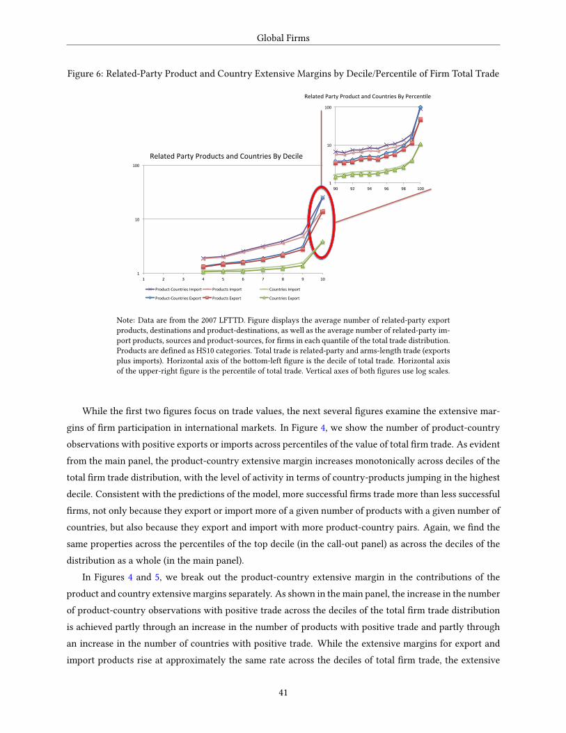
Global Firms
Figure 6: Related-Party Product and Country Extensive Margins by Decile/Percentile of Firm Total Trade
RelatedPartyProductsandCountriesByDecile
RelatedPartyProductandCountriesByPercenEle
1
10
100
1 2 3 4 5 6 7 8 9 10
Product-CountriesImport ProductsImport CountriesImport
Product-CountriesExport ProductsExport CountriesExport
1
10
100
90 92 94 96 98 100
Note: Data are from the 2007 LFTTD. Figure displays the average number of related-party export
products, destinations and product-destinations, as well as the average number of related-party im-
port products, sources and product-sources, for rms in each quantile of the total trade distribution.
Products are dened as HS10 categories. Total trade is related-party and arms-length trade (exports
plus imports). Horizontal axis of the bottom-left gure is the decile of total trade. Horizontal axis
of the upper-right gure is the percentile of total trade. Vertical axes of both gures use log scales.
While the rst two gures focus on trade values, the next several gures examine the extensive mar-
gins of rm participation in international markets. In Figure 4, we show the number of product-country
observations with positive exports or imports across percentiles of the value of total rm trade. As evident
from the main panel, the product-country extensive margin increases monotonically across deciles of the
total rm trade distribution, with the level of activity in terms of country-products jumping in the highest
decile. Consistent with the predictions of the model, more successful rms trade more than less successful
rms, not only because they export or import more of a given number of products with a given number of
countries, but also because they export and import with more product-country pairs. Again, we nd the
same properties across the percentiles of the top decile (in the call-out panel) as across the deciles of the
distribution as a whole (in the main panel).
In Figures 4 and 5, we break out the product-country extensive margin in the contributions of the
product and country extensive margins separately. As shown in the main panel, the increase in the number
of product-country observations with positive trade across the deciles of the total rm trade distribution
is achieved partly through an increase in the number of products with positive trade and partly through
an increase in the number of countries with positive trade. While the extensive margins for export and
import products rise at approximately the same rate across the deciles of total rm trade, the extensive
41

Global Firms
margin for export destinations rises more rapidly than that for import source countries, suggesting that
xed sourcing costs are large relative to xed exporting costs. For all these extensive margins, the level of
activity jumps for the top decile, and the distributions are fractal, in the sense that we observe a similar
pattern across percentiles of the top decile as across the deciles of the distribution as a whole.
Figure 6 shows the distribution of the extensive margins for related-party trade. The pattern is a
familiar one with a roughly log-linear increase across the deciles until the largest decile where there is a
substantial jump in activity. Again, we see the pattern repeated within the top decile, as the largest trading
rms have many more related-party connections for both imports and exports. This extensive margin of
related-party activity suggests a useful extension of our framework to incorporate the decision whether
to organize overseas production within the boundaries of the rm (foreign direct investment (FDI)) or
through arms-length transactions (outsourcing). Work on rm-level FDI has consistently found that more
productive rms are more likely to be multinationals, i.e. have at least one foreign aliate, and that the
numbers of host countries and aliates are increasing in measures of rm performance.39
Figure 7 shows that the largest trading rms account for larger shares of exports for individual product
markets. The average export market share of a rm’s top product in each market rises systematically across
deciles and percentiles of total trade. The largest rms in terms of total trade have average shares of US
exports for their top product within each market of 25 percent, while rms in the fth decile average under
7 percent of US exports of their top product within each market. In our model, such variation in market
shares gives rise to strategic market power, and generates variation in markups across rms.
39The large literature on foreign direct investment (FDI) includes Antràs (2003), Antràs and Helpman (2004), Arkolakis, Ra-
mondo, Rodriguez-Clare, and Yeaple (2015), Becker and Muendler (2010), Brainard (1997), Cravino and Levchenko (2015), Doms
and Jensen (1998), Hanson, Mataloni, and Slaughter (2005), Helpman (1984), Helpman, Melitz, and Yeaple (2004), Markusen and
Venables (1998, 2000), Ramondo and Rodriguez-Clare (2013), and Yeaple (2009), as reviewed in Antràs and Yeaple (2009).
42

Global Firms
Figure 7: Average Shares of a Firm’s Top Product in US Exports of that Product across Markets by
Decile/Percentile of Firm Total Trade
Note: Data are from the 2007 LFTTD. Figure displays the average across markets of the share of
a rm’s top product in US exports of that product to that market. We allow the denition of top
product to vary across markets. We display this average for rms in each quantile of the total trade
distribution. Total trade is related-party and arms-length trade (exports plus imports). Horizontal
axis of the bottom-left gure is the decile of total trade. Horizontal axis of the upper-right gure is
the percentile of total trade. Vertical axes of both gures are fractions.
Taken together, the results of this section provide further evidence in support of the predictions of
our theoretical model. All the margins of rm international participation strongly co-move together, with
greater participation along one margin correlated with more active engagement along another. In the
model, these correlations are driven by two mechanisms. On the one hand, higher rm productivity propels
greater international participation along all margins simultaneously, because of the non-random selection
of rms into these dierent activities. On other hand, the decisions to participate in international markets
along each margin are complementary with one another. As more productive rms incur the xed export-
ing costs of serving additional markets, this increases their production scale, and raises the protability
of incurring the xed importing costs for additional countries. Incurring these additional xed importing
costs in turn reduces production costs, which raises the protability of incurring the xed exporting costs
for additional markets. Through these forces of selection and complementarity, exogenous dierences
across rms are magnied, such that a relatively small number of rms account for a disproportionately
large share of aggregate trade.
43

Global Firms
Table
9:
Valu
es
an
dco
un
ts
by
Decile/P
ercen
tile
of
th
eV
alu
eo
fT
otal
Trad
ein
2007
Trad
eE
xp
orts
Im
po
rts
All
Related
-R
elated
-P
ro
du
ct-
Related
-P
ro
du
ct-
Decile
Party
All
Party
Co
un
tries
Pro
du
cts
Co
un
tries
All
Party
Co
un
tries
Pro
du
cts
Co
un
tries
13,6
36
83
2,7
10
1.0
1.0
1.0
926
1.2
1.2
1.0
29,0
89
221
6,6
67
1.3
1.3
1.1
2,4
22
1.5
1.5
1.1
319,6
02
488
13,7
31
1.8
1.7
1.3
5,8
71
1.9
1.8
1.2
439,0
83
1,0
57
26,1
62
671
2.4
2.1
1.6
12,9
21
386
2.4
2.2
1.3
576,6
77
2,2
54
47,7
53
1,2
63
3.2
2.7
2.0
28,9
24
991
3.0
2.8
1.4
6154,4
24
5,3
31
90,2
74
2,4
53
4.5
3.5
2.6
64,1
49
2,8
79
4.0
3.6
1.6
7324,2
56
14,5
00
175,5
94
5,6
95
6.3
4.5
3.4
148,6
61
8,8
05
5.5
4.7
1.9
8733,3
26
42,0
46
367,2
18
13,3
58
9.0
5.9
4.4
366,1
09
28,6
88
7.3
6.0
2.3
92,0
65,1
89
182,8
97
936,9
88
49,7
75
13.7
8.3
6.0
1,1
28,2
01
133,1
22
11.1
8.6
3.0
10
88,0
61,6
48
39,9
84,7
64
32,0
75,3
18
10,5
15,4
36
56.2
23.4
12.8
55,9
86,3
28
29,4
69,3
26
42.0
23.0
6.6
Trad
eE
xp
orts
Im
po
rts
Related
-R
elated
-P
ro
du
ct-
Related
-P
ro
du
ct-
Percen
tile
All
Party
All
Party
Co
un
tries
Pro
du
cts
Co
un
tries
All
Party
Co
un
tries
Pro
du
cts
Co
un
tries
90
3,4
35,3
21
357,6
56
1,4
90,4
21
100,9
88
16.8
9.8
7.1
1,9
44,9
00
256,6
68
14.7
11.0
3.5
91
4,0
23,4
76
443,0
04
1,7
45,7
03
105,0
11
18.3
10.4
7.5
2,2
77,7
73
337,9
93
14.3
10.5
3.7
92
4,7
45,5
00
540,8
08
2,0
51,3
52
122,8
27
20.2
11.2
8.0
2,6
94,1
48
417,9
81
15.9
11.7
3.9
93
5,6
99,3
26
749,4
23
2,3
60,9
96
178,2
58
22.0
12.2
8.4
3,3
38,3
30
571,1
65
16.6
12.3
4.0
94
6,9
76,0
46
942,9
54
2,9
16,6
73
231,5
52
24.1
13.0
9.1
4,0
59,3
73
711,4
02
17.9
13.0
4.3
95
8,7
59,8
72
1,1
98,8
60
3,5
37,9
86
267,7
46
25.4
13.6
9.2
5,2
21,8
86
931,1
15
20.2
14.4
4.7
96
11,4
83,8
36
1,8
45,3
85
4,7
72,4
62
438,1
96
28.7
14.8
9.9
6,7
11,3
74
1,4
07,1
88
22.3
16.0
5.0
97
15,9
95,4
23
2,8
56,6
74
6,6
07,4
54
675,2
32
34.1
16.6
11.4
9,3
87,9
69
2,1
81,4
43
26.1
18.3
5.6
98
24,9
41,7
30
5,0
88,6
83
10,1
79,6
95
1,2
44,5
85
42.8
20.9
13.3
14,7
62,0
34
3,8
44,0
98
32.7
21.3
6.5
99
49,8
22,0
84
12,6
26,6
25
20,2
63,5
20
3,1
36,5
05
63.2
28.4
17.1
29,5
58,5
64
9,4
90,1
20
44.8
28.4
8.6
100
748,3
28,2
56
373,6
35,8
40
266,3
73,6
48
98,7
75,7
84
261.7
86.0
31.4
481,9
54,5
92
274,8
60,0
64
193.4
78.2
18.0
No
te:
Data
are
fro
mth
e2007
LFT
TD
.T
his
table
rep
orts
valu
es
an
dco
un
ts
by
decile
or
percen
tile
of
th
evalu
eo
fto
tal
trad
e.
To
tal
trad
eis
related
-
party
an
darm
s-len
gth
trad
e(exp
orts
plu
sim
po
rts).
Related
-p
arty
refers
to
trad
eb
etw
een
related
parties.
Pro
du
cts
co
rresp
on
dto
Harm
on
ized
Sy
stem
(H
S)
10-d
igit
pro
du
cts.
44

Global Firms
5 Conclusions
Over the last two decades, a growing body of theoretical and empirical research has demonstrated the
role of heterogeneous rm decisions in mediating the economy’s response to international trade. The
now-standard model of heterogeneous rms and trade envisions a continuum of measure zero rms that
compete under conditions of monopolistic competition and self-select into export markets. In this paper,
we review this research and argue that this standard paradigm does not go far enough in recognizing the
role of “global rms,” dened as rms that participate in the international economy along multiple margins
and account for substantial shares of aggregate trade.
We outline a theoretical framework that recognizes the role played by such global rms. We allow large
rms to internalize the eects of their choices on market aggregates, which results in variable markups,
pricing to market and incomplete pass-through. We include a much richer range of margins along which
rms can participate in international markets than the standard paradigm. Each rm can choose the set
of production locations in which to operate plants; the set of export markets for each plant; the set of
products to export from each plant to each market; the exports of each product from each plant to each
market; the set of countries from which to source intermediate inputs for each plant; and imports of each
intermediate input from each source country by each plant.
We use U.S. rm and trade transactions data to provide empirical evidence on the predictions of this
framework. Consistent with the selection forces in our model, we show that only a subset of rms partic-
ipate in international markets (through either exporting or importing) and that these trading rms have
superior performance characteristics: they are larger and more productive than purely domestic rms.
We nd strong support for our model’s prediction of a correlation between the dierent margins of rm
participation in the global economy. A substantial fraction of rms that export or import do both. More
successful rms export more of each product to each market, export more products to each market, ex-
port to more markets, import more of each product from each source country, importing more products
from each source country, and import from more source countries. These empirical ndings also pro-
vide support for the magnication eects emphasized in our model. Small dierences in exogenous rm
characteristics have amplied eects on endogenous rm performance (such as sales), because they are
magnied by these endogenous market participation decisions, thereby helping to explain how a relatively
small number of rms dominate aggregate international trade.
While much already has been achieved within the literature on heterogeneous rms and trade, there
remains much to be done. Recognizing the importance of global rms opens up a number of avenues for
further research, including their implications for the transmission of international shocks, the elasticity
of trade with respect to trade costs, and the aggregate welfare gains from trade. Although we consider
many margins of rm participation in the international economy, we abstract from the decision whether
to organize global production chains within or beyond the boundaries of the rm, which itself has been
45

Global Firms
the subject of much recent research. Therefore another interesting area for further inquiry is exploring
the implications of this internalization decision for rm performance and country comparative advantage
in a world of such global rms.
46

Global Firms
A Appendix
A.1 Derivation of Equilibrium Pricing Rule
The rst-order condition for the price of product k for rm f from production country i in market m within
sector g is:
QKmik + ∑
h∈ΩKmi f
PKmih
∂QKmih
∂PKmik−
dXmiw
αgi
(γK
k
)1−αg[Φi f h
(ΩNI
i f
)]− 1−αgθKk
ϕi f
∂QKmih
∂PKmik
= 0. (30)
From equation (9), we have:
∂QKmih
∂PKmik
=(
σFg − 1
) QKmih
PGmg
∂PGmg
∂PKmik
+(
σKg − σF
g
) QKmih
PFmi f
∂PFmi f
∂PKmik− σK
gQK
mih
PKmik
∂PKmih
∂PKmik
.
We now can use the expenditure shares (7) and (8) to solve for the elasticities and rewrite ∂QKmih/∂PK
mik as
∂QKmih
∂PKmik
=(
σFg − 1
)( ∂PGmg
∂PFmi f
PFmi f
PGmg
)(∂PF
mi f
∂PKmik
PKmik
PFmi f
)QK
mihPK
mik+(
σKg − σF
g
)( ∂PFmi f
∂PKmik
PKmik
PFmi f
)QK
mihPK
mik− σK
gQK
mihPK
mik1k=h
=(
σFg − 1
)SF
mi f SKmik
QKmih
PKmik
+(
σKg − σF
g
)SK
mikQK
mihPK
mik− σK
gQK
mihPK
mik1k=h. (31)
If we now substitute equation (31) into equation (30) and divide both sides by QKmik, we get:
1 + ∑h∈ΩK
mi f
(σF
g − 1)
SFmi f SK
mikPK
mihQKmih
PKmikQK
mik+ ∑
h∈ΩKmi f
(σK
g − σFg
)SK
mikPK
mihQKmih
PKmikQK
mik− σK
g
− ∑h∈ΩK
mi f
(σF
g − 1)
SFmi f SK
mik
dXmiw
αgi (γK
k )1−αg
[Φi f h
(ΩNI
i f
)]− 1−αgθKk
ϕi fQK
mih
PKmikQK
mik− ∑
h∈ΩKmi f
(σK
g − σFg
)SK
mik
dXmiw
αgi (γK
k )1−αg
[Φi f h
(ΩNI
i f
)]− 1−αgθKk
ϕi fQK
mih
PKmikQK
mik(32)
+σKg
dXmiw
αgi (γK
k )1−αg
[Φi f k
(ΩNI
i f
)]− 1−αgθKk
ϕi f
PKmik
= 0.
We dene the markup as µKmih ≡ PK
mih(
dXmiw
αgi
(γK
k
)1−αg[Φi f h
(ΩNI
i f
)]− 1−αgθKk /ϕi f
). Since SK
mik1
PKmikYK
mik=
1∑h∈ΩK
mi fPK
mihYKmih
and therefore ∑h∈ΩKmi f
SKmik
PKmihYK
mihPK
mikYKmik
= 1, we can rewrite equation (32) as:
[1 +
(σF
g − 1)
SFmi f +
(σK
g − σFg
)− σK
g
]−(
σFg − 1
)SF
mi f
∑h∈ΩK
mi f
dXmiw
αgi (γK
k )1−αg
[Φi f h
(ΩNI
i f
)]− 1−αgθKk
ϕi fQK
mih
∑h∈ΩK
mi f
PKmihQK
mih
−(
σKg − σF
g
) ∑h∈ΩK
mi f
dXmiw
αgi (γK
k )1−αg
[Φi f h
(ΩNI
i f
)]− 1−αgθKk
ϕi fQK
mih
∑h∈ΩK
mi f
PKmihQK
mih+ σK
g1
µKmik
= 0.
47

Global Firms
Note that µKmik is the only k-specic term in this expression. Hence, µK
mik must take the same value for all
products k supplied by rm f from production country i to market m within sector g: µKmik = µF
mi f for all
k ∈ ΩKmi f . In other words, markups are the same across products within a given rm, market and sector. We
can now solve for µFmi f using:[
1 +(
σFg − 1
)SF
mi f +(
σKg − σF
g
)− σK
g
]−(
σFg − 1
)SF
mi f1
µFmi f−(
σKg − σF
g
) 1µF
mi f+ σK
g1
µFmi f
= 0
⇒ µFmi f =
σFg −
(σF
g − 1)
SFmi f
σFg −
(σF
g − 1)
SFmi f − 1
.
A.2 Proof of Proposition 1
Proof. (i) From the rm price index (6) and rm pricing rule (20), we have:
PFmi f =
(µF
mi f
ϕi f
)ΓF
mi f , (33)
where
ΓFmi f = dX
miwαgi
∑k∈ΩK
mi f
(γK
k
)1−αg[Φi f k
(ΩNI
i f
)]− 1−αgθKk
λKmik
1−σK
g
11−σK
g
,
Φi f k
(ΩNI
i f
)≡ ∑
j∈ΩNIi f
TKjk(wjdI
ij)−θK
k .
Using the rm expenditure share (7) and (33), we obtain:
SFmi f =
(µF
mi f /ϕi f
)1−σFg(
ΓFmi f /λF
mi f
)1−σFg
∑i∈ΩN
∑o∈ΩF
mig
(µF
mio/ϕio)1−σF
g(ΓF
mio/λFmio
)1−σFg
. (34)
Using the mark-up (21) and perceived elasticity (22), we dene the following implicit function:
Ξ = SFmi f −
(σF
g−(σFg−1)SF
mi f
(σFg−1)−(σF
g−1)SFmi f
)1−σFg
ϕσF
g−1i f
(ΓF
mi f /λFmi f
)1−σFg
∑i∈ΩN
∑o∈ΩF
mig
(σF
g−(σFg−1)SF
mio
(σFg−1)−(σF
g−1)SFmio
)1−σFg
ϕσF
g−1io
(ΓF
mio/λFmio
)1−σFg
= 0. (35)
From the implicit function theorem:
∂SFmi f
∂ϕi f= −
∂Ξ/∂ϕi f
∂Ξ/∂SFmi f
, (36)
where we hold constant wm, ΩNPf , ΩNX
i f , ΩNIi f , ΩK
mi f and all other model parameters except productivity.
From (35), we have:
∂Ξ∂ϕi f
= −σF
g − 1ϕi f
SFmi f
(1− SF
mi f
)< 0, (37)
48

Global Firms
∂Ξ∂SF
mi f= 1 +
(σF
g − 1)(∂µF
mi f
∂SFmi f
SFmi f
µFmi f
)(1− SF
mi f
)> 0, (38)
since
∂µFmi f
∂SFmi f
SFmi f
µFmi f
=σF
g − 1
εFmi f − 1
SFmi f
(1− 1
µFmi f
)> 0. (39)
From (36)-(39), an increase in rm productivity raises expenditure shares within each market:
∂SFmi f
∂ϕi f> 0, (40)
(ii) Together (39) and (40) imply that an increase in rm productivity raises markups:
∂µFmi f
∂ϕi f> 0. (41)
From (34), the rm expenditure share is decreasing in the ratio of the markup to rm productivity (µFmi f /ϕi f ):
∂SFmi f
∂(
µFmi f /ϕi f
) = −σF
g − 1(µF
mi f /ϕi f
)SFmi f
(1− SF
mi f
)< 0. (42)
Now we combine (40)-(42). The rm expenditure share increases in productivity in (40), even though the
rm markup increases in productivity in (41). Therefore, from (42), the rm markup must rise less than
proportionately with productivity (to ensure that the rm expenditure share increases in productivity),
which implies that the price of each product must decrease in productivity:
∂PKmik
∂ϕi f=
∂
(µF
mi fϕi f
dXmiw
αgi
(γK
k
)1−αg[Φi f k
(ΩNI
i f
)]− 1−αgθKk
)∂ϕi f
< 0. (43)
(iii) Sales of each product in each sector in each market can be written as:
EKmik = SK
mikSKmi f
(λG
mgwmLm
), (44)
where the share of each product k in rm expenditure (SKmik) is independent of rm productivity and the
markup because both are common across products within a given rm in a given market:
SKmik =
((γK
k
)1−αg[Φi f k
(ΩNI
i f
)]− 1−αgθKk /λK
mik
)1−σKg
∑n∈ΩK
mi f
((γK
k
)1−αg[Φi f n
(ΩNI
i f
)]− 1−αgθKk /λK
min
)1−σKg
. (45)
From (40), (44) and (45), the rm expenditure share (SKmi f ) increases in rm productivity, while the product
expenditure share (SKmik) is unaected by rm productivity. Therefore an increase in rm productivity
raises sales of each product in a given market:
∂EKmik
∂ϕi f> 0. (46)
49

Global Firms
Output of each product in a given sector and market can be written as:
QKmik =
EKmik
PKmik
. (47)
From (43) and (46), an increase in rm productivity raises sales (EKmik) and reduces (PK
mik) of each product
in each market, which implies that it raises output (QKmik) of each product in each market:
∂QKmik
∂ϕi f> 0. (48)
Since an increase in rm productivity raises sales and output of each product in each market, it also raises
overall sales (EKik) and output (QK
ik) of each product across all markets:
∂EKik
dϕi f> 0,
∂QKik
∂ϕi f> 0, (49)
where EKik = ∑m∈ΩNX
i fEK
mik and QKik = ∑m∈ΩNX
i fQK
mik.
A.3 Proof of Proposition 2
Proof. From Proposition 1, we have:
∂EKmik
∂ϕi f> 0,
∂µFmi f
∂ϕi f> 0,
where we hold constant wm, ΩNPf , ΩNX
i f , ΩNIi f , ΩK
mi f , ΩKmi f and all model parameters except productivity.
Therefore we have:
∂
((µF
mi f−1
µFmi f
)EK
mik
)∂ϕi f
> 0, for all k ∈
ΩKmi f \ΩK
mi f
,
which together with (27) establishes the proposition.
A.4 Proof of Proposition 3
Proof. From Proposition 1, we have:
∂EKmik
∂ϕi f> 0,
∂µFmi f
∂ϕi f> 0,
where we hold constant wm, ΩNPf , ΩNX
i f , ΩNIi f , ΩK
mi f , ΩKmi f and all model parameters except productivity.
Therefore we have:
∂
((µF
mi f−1
µFmi f
)EK
mik
)∂ϕi f
> 0, for all k ∈ ΩKmi f ,
which together with (28) establishes the proposition.
50
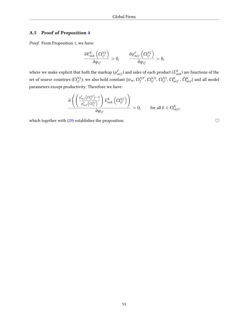
Global Firms
A.5 Proof of Proposition 4
Proof. From Proposition 1, we have:
∂EKmik
(ΩNI
i f
)∂ϕi f
> 0,∂µF
mi f
(ΩNI
i f
)∂ϕi f
> 0,
where we make explicit that both the markup (µFmi f ) and sales of each product (EK
mik) are functions of the
set of source countries (ΩNIi f ); we also hold constant wm, ΩNP
f , ΩNXi f , ΩNI
i f , ΩKmi f , ΩK
mi f and all model
parameters except productivity. Therefore we have:
∂
((µF
mi f
(ΩNI
i f
)−1
µFmi f
(ΩNI
i f
))
EKmik
(ΩNI
i f
))∂ϕi f
> 0, for all k ∈ ΩKmi f ,
which together with (29) establishes the proposition.
51

Global Firms
References
Abowd, J. M., R. H. Creecy, and F. Kramarz (2002): “Computing Person and Firm Eects Using Linked
Longitudinal Employer-Employee Data,” LEHD Technical Paper, 2002-06.
Abowd, J. M., F. Kramarz, and D. N. Margolis (1999): “High Wage Workers and High Wage Firms,”
Econometrica, 67(2), 251–333.
Ahn, J., A. Khandelwal, and S. Wei (2011): “The Role of Intermediaries in Facilitating Trade,” Journal of
International Economics, 84(1), 73–85.
Akerman, A. (2010): “Wholesalers and Economies of Scope in International Trade,” Research Papers in
Economics, Department of Economics, Stockholm University 2010:1.
Alfaro, L., P. Antrás, D. Chor, and P. Conconi (2015): “Internalizing Global Value Chains: A Firm-Level
Analysis,” NBER Working Paper, 21582.
Amiti, M., and D. R. Davis (2011): “Trade, Firms and Wages: Theory and Evidence,” Review of Economic
Studies, 79(1), 1–36.
Amiti, M., O. Itskhoki, and J. Konings (2014): “Importers, Exporters and Exchange Rate Disconnect,”
American Economic Review, 104(7), 1942–1978.
Amiti, M., and J. Konings (2007): “Trade Liberalization, Intermediate Inputs, and Productivity: Evidence
from Indonesia,” American Economic Review, 97(5), 1611–1638.
Antràs, P. (2003): “Firms, Contracts, and Trade Structure,” Quarterly Journal of Economics, 118(4), 1375–
1418.
(2015): Global Production: Firms, Contracts, and Trade Structure. Princeton University Press, Prince-
ton.
Antràs, P., and D. Chor (2013): “Organizing the Global Value Chain,” Econometrica, 81(6), 2127–2204.
Antràs, P., and A. Costinot (2011): “Intermediated Trade,” Quarterly Journal of Economics, 126(3), 1319–
1374.
Antràs, P., T. Fort, and F. Tintelnot (2014): “The Margins of Global Sourcing: Theory and Evidence
from U.S. Firms,” Harvard University, mimeograph.
Antràs, P., and E. Helpman (2004): “Global Sourcing,” Journal of Political Economy, 112(3), 552–80.
Antràs, P., and E. Rossi-Hansberg (2009): “Organizations and Trade,” Annual Review of Economics, 1,
43–64.
52

Global Firms
Antràs, P., and S. Yeaple (2009): “Multinational Firms and the Structure of International Trade,” in Hand-
book of International Trade, ed. by G. Gopinath, E. Helpman, and K. Rogo, vol. 4, chap. 2, pp. 55–130.
Elsevier North Holland, Amsterdam.
Arkolakis, C., A. Costinot, and A. Rodriguez-Clare (2012): “New Trade Models, Same Old Gains,”
American Economic Review, 102(1), 94–130.
Arkolakis, C., M. A. Muendler, and S. Ganapati (2014): “The Extensive Margin of Exporting Products:
A Firm-Level Analysis,” NBER Working Paper, 16641.
Arkolakis, C., N. Ramondo, A. Rodriguez-Clare, and S. Yeaple (2015): “Innovation and Production in
the Global Economy,” Yale University, mimeograph.
Armenter, R., andM. Koren (2014): “A Balls-and-Bins Model of Trade,” American Economic Review, 104(7),
2127–2151.
Atalay, E., A. Hortaçsu, and C. Syverson (2014): “Vertical Integration and Input Flows,” American Eco-
nomic Review, 104(4), 1120–48.
Atkeson, A., and A. Burstein (2008): “Pricing to Market, Trade Costs and International Relative Prices,”
American Economic Review, 98(5), 1998–2031.
Atkeson, A., and A. T. Burstein (2010): “Innovation, Firm Dynamics, and International Trade,” Journal
of Political Economy, 118(3), 433–484.
Axtell, R. (2001): “Zipf Distribution of U.S. Firm Sizes,” Science, 293, 1818–1820.
Baldwin, R., and A. Venables (2013): “Spiders and Snakes: O-shoring and Agglomeration in the Global
Economy,” Journal of International Economics, 90, 245–254.
Baumgarden, D. (2013): “Exporters and the Rise in Wage Inequality: Evidence from German Linked
Employer-Employee Data,” Journal of International Economics, 90(1), 201–217.
Becker, S. O., andM.Muendler (2010): “Margins of Multinational Labor Substitution,” American Economic
Review, 100(5), 1999–2030.
Behrens, K., and Y. Murata (2012): “Trade, Competition, and Eciency,” Journal of International Eco-
nomics, 87(1), 1–17.
Bergin, P., and R. Feenstra (2001): “Pricing-to-Market, Staggered Contracts and Real Exchange Rate
Persistence,” Journal of International Economics, 44, 333–359.
53

Global Firms
Berman, N., P. Martin, and T. Mayer (2012): “How do Dierent Exporters React to Exchange Rate
Changes? Theory, Empirics and Aggregate Implications,” Quarterly Journal of Economics, 127(1), 437–
492.
Bernard, A. B., E. J. Blanchard, I. V. Beveren, andH. Vandenbusshe (2015): “Carry-Along Trade,” Tuck
School of Business at Dartmouth.
Bernard, A. B., J. Eaton, J. B. Jensen, and S. S. Kortum (2003): “Plants and Productivity in International
Trade,” American Economic Review, 93(4), 1268–1290.
Bernard, A. B., and T. Fort (2015): “Factoryless Goods Producing Firms,” American Economic Review,
forthcoming.
Bernard, A. B., M. Grazzi, and C. Tomasi (2014): “Intermediaries in International Trade: Margins of
Trade and Export Flows,” NBER Working Paper, 17711.
Bernard, A. B., and J. B. Jensen (1995): “Exporters, Jobs, and Wages in US Manufacturing: 1976-87,”
Brookings Papers on Economic Activity: Microeconomics, pp. 67–112.
(1999): “Exceptional Export Performance: Cause, Eect or Both?,” Journal of International Eco-
nomics, 47(1), 1–25.
Bernard, A. B., J. B. Jensen, S. J. Redding, and P. K. Schott (2007): “Firms in International Trade,” Journal
of Economic Perspectives, 21(3), 105–130.
(2009): “The Margins of U.S. Trade,” American Economic Review, 99(2), 487–493, Papers and Pro-
ceedings.
(2010a): “Intra-rm Trade and Product Contractibility,” American Economic Review, 100(2), 444–
448, Papers and Proceedings.
(2010b): “Wholesalers and Retailers in U.S. Trade,” American Economic Review, 100(2), 408–413,
Papers and Proceedings.
(2012): “The Empirics of Firm Heterogeneity and International Trade,” Annual Review of Economics,
4, 283–313.
Bernard, A. B., J. B. Jensen, and P. K. Schott (2009): “Importers, Exporters and Multinationals: A Portrait
of Firms in the U.S. that Trade Goods,” in Producer Dynamics: New Evidence from Micro Data, ed. by
T. Dunne, J. B. Jensen, and M. J. Roberts. Chicago University Press, Chicago.
Bernard, A. B., A. Moxnes, and Y. Saito (2014): “Production Networks, Geography and Firm Perfor-
mance,” Tuck School of Business at Dartmouth, mimeograph.
54

Global Firms
Bernard, A. B., A. Moxnes, and K. H. Ulltveit-Moe (2015): “Two-sided Heterogeneity and Trade,” Tuck
School of Business at Dartmouth, unpublished.
Bernard, A. B., S. J. Redding, and P. K. Schott (2007): “Comparative Advantage and Heterogeneous
Firms,” Review of Economic Studies, 74(1), 31–66.
(2010): “Multi-product Firms and Product Switching,” American Economic Review, 100(1), 70–97.
(2011): “Multiproduct Firms and Trade Liberalization,” Quarterly Journal of Economics, 126(3),
1271–1318.
Bernard, A. B., V. Smeets, and F. Warzynski (2016): “Rethinking Deindustrialization,” NBER Working
Paper, 22114.
Bernard, A. B., and J.Wagner (1997): “Exports and Success in German Manufacturing,”Weltwirtschaftliches
Archiv, 133(1), 134–157.
Berry, S. T. (1994): “Estimating Discrete-choice Models of Product Dierentiation,” RAND Journal of Eco-
nomics, 25, 242–262.
Blaum, J., C. Lelarge, and M. Peters (2013): “Non-Nomothetic Import Demand: Firm Productivity and
Quality Bias,” Brown University, mimeograph.
(2014): “Estimating the Productivity Gains from Importing,” Brown University, mimeograph.
Blum, B., S. Claro, and I. Horstmann (2000): “Facts and Figures on Intermediated Trade,” American
Economic Review, 100(2), 419–423, Papers and Proceedings.
Boehm, Christoph E., A. F., and N. Pandalai-Nayar (2015): “Multinationals, Oshoring, and the Decline
of U.S. Manufacturing?,” .
Brainard, S. L. (1997): “An Empirical Assessment of the Proximity-Concentration Trade-o between
Multinational Sales and Trade,” American Economic Review, 87(4), 520–544.
Breinlich, H., and C. Criscuolo (2011): “International Trade in Services: A Portrait of Importers and
Exporters,” Journal of International Economics, 84(2), 188–206.
Bresnahan, T. (1989): “Empirical Studies of Industries with Market Power,” in Handbook of Industrial
Organization, ed. by R. Schmalensee, and R. Willig, vol. 2. Elsevier, North Holland, Amsterdam.
Broda, C., and D. E. Weinstein (2010): “Product Creation and Destruction: Evidence and Price Implica-
tions,” American Economic Review, 691-723.
55

Global Firms
Brooks, E. (2006): “Why Don’t Firms Export More? Product Quality and Colombian Plants,” Journal of
Development Economics, 80, 160–178.
Burstein, A., and J. Vogel (2015): “International Trade, Technology, and the Skill Premium,” Columbia
University, mimeograph.
Bustos, P. (2011): “Trade Liberalization, Exports and Technology Upgrading: Evidence on the impact of
MERCOSUR on Argentinian Firms,” American Economic Review, 101(1), 304–340.
Caves, D. W., L. R. Christensen, and W. E. Diewert (1982): “The Economic Theory of Index Numbers
and the Measurement of Input, Output, and Productivity,” Econometrica, 50(6), 1393–1414.
Chaney, T. (2008): “Distorted Gravity: The Intensive and Extensive Margins of International Trade,” Amer-
ican Economic Review, 98(4), 1707–1721.
(2014): “The Network Structure of International Trade,” American Economic Review, 104(11), 3600–
3634.
(2015): “The Gravity Equation in International Trade: An Explanation,” Toulouse School of Eco-
nomics, mimeograph.
Cherkashin, I., S. Demidova, H. L. Kee, and K. Krishna (2010): “Firm Heterogeneity and Costly Trade:
A New Estimation Strategy and Policy Experiments,” Penn State, mimeograph.
Clerides, Sofronis, S. L., and J. Tybout (1998): “Is Learning by Exporting Important? Micro-dynamic
Evidence from Columbia, Mexico and Morocco,” Quarterly Journal of Economics, 113(3), 903–947.
Constantini, J. A., and M. J. Melitz (2008): “The Dynamics of Firm-Level Adjustment to Trade Liberal-
ization,” in The Organization of Firms in a Global Economy, ed. by E. Helpman, D. Marin, and T. Verdier,
pp. 107–141. Harvard University Press, Princeton.
Corcos, G., M. Del Gatto, G. Mion, and G. Ottaviano (2012): “Productivity and Firm Selection: Quan-
tifying the New Gains from Trade,” Economic Journal, 122(561), 754–798.
Costinot, A., J. Vogel, and S. Wang (2013): “An Elementary Theory of Global Supply Chains,” Review of
Economic Studies, 80, 109–144.
Cravino, J., and A. Levchenko (2015): “Multinational Firms and International Business Cycle Transmis-
sion,” University of Michigan, mimeograph.
Davidson, C., F. Heyman, S. Matusz, F. Sjöholm, and S. C. Zhu (2014): “Globalization and Imperfect
Labor Market Sorting,” Journal of International Economics, 94(2), 177–94.
56

Global Firms
De Loecker, J. (2007): “Do Exports Generate Higher Productivity? Evidence from Slovania,” Journal of
International Economics, 73, 69–98.
De Loecker, J., and P. Goldberg (2014): “Firm Performance in a Global Market,” Annual Review of Eco-
nomics, 6, 201–227.
De Loecker, J., P. Goldberg, A. Khandelwal, and N. Pavcnik (2015): “Prices, Markups and Trade Re-
form,” Econometrica, forthcoming.
De Loecker, J., and F. Warzynski (2012): “Markups and Firm-level Export Status,” American Economic
Review, 102(6), 2437–2471.
Dhingra, S. (2013): “Trading Away Wide Brands for Cheap Brands,” American Economic Review, 103(6),
2554–84.
Di Comite, F., J.-F. Thisse, andH. Vandenbussche (2014): “Verti-zontal dierentiation in export markets,”
Journal of International Economics, 93(1), 50–66.
di Giovanni, J., A. Levchenko, and I. Mejean (2014): “Firms, Destinations, and Aggregate Fluctuations,”
Econometrica, 82(4), 1303–1340.
Dixit, A., and G. M. Grossman (1982): “Trade and Protection with Multi-Stage Production,” Review of
Economic Studies, 49(4), 583–94.
Doms, M. E., and J. . B. Jensen (1998): “Comparing Wages, Skills, and Productivity between Domestically
and Foreign-Owned Manufacturing Establishments in the United States,” in Geography and Ownership
as Bases for Economic Accounting, pp. 235–258. Chicago University Press, Chicago.
Eaton, J., D. Jinkins, J. Tybout, and D. Xu (2016): “Two Sided Search in International Markets,” Penn
State University, mimeograph.
Eaton, J., and S. Kortum (2002): “Technology, Geography, and Trade,” Econometrica, 70(5), 1741–1779.
Eaton, J., S. Kortum, F. Kramarz, and R. Sampognaro (2014): “Firm-to-Firm Trade: Imports, Exports,
and the Labor Market,” Yale University, mimeograph.
Eaton, J., S. Kortum, and S. Sotelo (2012): “International Trade: Linking the Micro and the Macro,” NBER
Working Paper, 17864.
Eaton, J., S. S. Kortum, and F. Kramarz (2004): “Dissecting Trade: Firms, Industries, and Export Desti-
nations,” American Economic Review, 94(2), 150–154, Papers and Proceedings.
(2011): “An Anatomy of International Trade: Evidence from French Firms,” Econometrica, pp.
1453–1498.
57

Global Firms
Eckel, C., and P. J. Neary (2010): “Multi-product Firms and Flexible Manufacturing in the Global Econ-
omy,” Review of Economic Studies, 77, 188–217.
Edmond, C., V. Midrigan, and D. Y. Xu (2012): “Competition, Markups, and the Gains from International
Trade,” NBER Working Paper, 18041.
Feenstra, R., andH. Ma (2008): “Optimal Choice of Product Scope for Multiproduct Firms,” in The Organi-
zation of Firms in a Global Economy, ed. by D. M. Elhanan Helpman, and T. Verdier, chap. 6, pp. 173–199.
Harvard University Press, Cambridge MA.
Feenstra, R. C., and J. Romalis (2014): “International Prices and Endogenous Quality,” Quarterly Journal
of Economics, 129(2), 477–527.
Fitzgerald, D., and S. Haller (2015): “Pricing-to-Market: Evidence from Plant-Level Prices,” Review of
Economic Studies, forthcoming.
Freund, C., andM. D. Pierola (2015): “Export Superstars,” Review of Economics and Statistics, 97(5), 1023–
1032.
Frías, J. A., D. S. Kaplan, and E. A. Verhoogen (2015): “Exports and Wage Premia: Evidence from Mexican
Employer-Employee Data,” Columbia University, unpublished manuscript.
Gabaix, X. (2011): “The Granular Origins of Aggregate Fluctuations,” Econometrica, 79, 733–772.
Gaubert, C., and O. Itskhoki (2015): “Granular Comparative Advantage,” Princeton University, mimeo-
graph.
Girma, S., D. Greenaway, and R. Kneller (2004): “Does Exporting Increase Productivity?: a Microecono-
metric Analysis of Matched Firms,” Review of International Economics, 12(5), 855–866.
Goldberg, P. (1995): “Product Dierentiation and Oligopoly in International Markets: The Case of the US
Automobile Industry,” Econometrica, 63, 891–951.
Goldberg, P., and R. Hellerstein (2013): “A Structural Approach to Identifying the Sources of Local-
Currency Price Stability,” Review of Economic Studies, 80, 175–210.
Goldberg, P., A. Khandelwal, N. Pavcnik, and P. Topalova (2010): “Imported Intermediate Inputs and
Domestic Product Growth: Evidence from India,” Quarterly Journal of Economics, 125(4), 1727–67.
Goldberg, P., and M. Knetter (1997): “Goods Prices and Exchange Rates: What Have We Learned?,”
Journal of Economic Literature, 35(3), 1243–1272.
Gopinath, G., and O. Itskhoki (2010): “Frequency of Price Adjustment and Pass-through,” Quarterly
Journal of Economics, 125(2), 675–727.
58

Global Firms
Grossman, G. M. (2013): “Heterogeneous Workers and International Trade,” Review of World Economics,
149(2), 211–245.
Grossman, G. M., and E. Rossi-Hansberg (2008): “Trading Tasks: A Simple Theory of Oshoring,” Amer-
ican Economic Review, 98(5), 1978–97.
Hallak, J. C., and P. K. Schott (2011): “Estimating Cross-Country Dierences in Product Quality,” Quar-
terly Journal of Economics, 126(1), 417–474.
Halpern, L., M. Koren, and A. Szeidl (2015): “mported Inputs and Productivity,” American Economic
Review.
Hanson, G. H., R. Mataloni, and M. Slaughter (2005): “Vertical Production Networks in Multinational
Firms,” Review of Economics and Statistics, 87, 664–678.
Harrigan, J., and A. Reshef (2015): “Skill-biased Heterogeneous Firms, Trade Liberalization and the Skill
Premium,” Canadian Journal of Economics.
Helpman, E. (1984): “A Simple Theory of International Trade with Multinational Corporations,” Journal
of Political Economy, 92(3), 451–471.
(2006): “Trade, FDI and the Organization of Firms,” Journal of Economic Literature, 44(3), 589–630.
Helpman, E., O. Itskhoki, M. A. Muendler, and S. J. Redding (2016): “Trade and Inequality: From Theory
to Estimation,” Review of Economic Studies, forthcoming.
Helpman, E., O. Itskhoki, and S. J. Redding (2010): “Inequality and Unemployment in a Global Economy,”
Econometrica, 78(4), 1239–1283.
Helpman, E., M. J. Melitz, and Y. Rubinstein (2008): “Estimating Trade Flows: Trading Partners and
Trading Volumes,” Quarterly Journal of Economics, 123(2), 441–87.
Helpman, E., M. J. Melitz, and S. R. Yeaple (2004): “Export Versus FDI with Heterogeneous Firms,” Amer-
ican Economic Review, 94(1), 300–316.
Holmes, J., and J. J. Stevens (2012): “Exports, Borders, Distance and Plant Size,” Journal of International
Economics, 88(1), 91–103.
Hornok, C., andM. Koren (2014): “Per-Shipment Costs and the Lumpiness of International Trade,” Review
of Economics and Statistics, forthcoming.
(2015): “Administrative Barriers to Trade,” Journal of International Economics, forthcoming.
59

Global Firms
Hottman, C., S. Redding, and D. Weinstein (2016): “Quantifying the Sources of Firm Heterogeneity,”
Quarterly Journal of Economics, 131(3), 1291–1364.
Hsieh, C.-T., and R. Ossa (2011): “A Global View of Productivity Growth in China,” NBER Working Paper,
16778.
Irarrazabal, A., L. Opromolla, and A. Moxnes (2013): “The Margins of Multinational Production and
the Role of Intrarm Trade,” Journal of Political Economy, 121(1), 74–126.
Jarmin, R. S., and J. Miranda (2002): “The Longitudinal Business Database,” Center for Economic Studies
Working Paper, 02(17).
Johnson, R. C., and G. Noguera (2012): “Fragmentation and Trade in Value Added over Four Decades,”
NBER Working Paper, 18186.
Kasahara, H., and B. Lapham (2008): “Productivity and the Decision to Import and Export: Theory and
Evidence,” CESifo Working Paper, 2240.
Kehoe, T. J., and K. J. Ruhl (2013): “How Important Is the New Goods Margin in International Trade?,”
Journal of Political Economy, 121(2), 358–392.
Khandelwal, A. (2010): “The Long and Short (of) Quality Ladders,” Review of Economic Studies, 77(4),
1450–1476.
Krishna, P., J. P. Poole, andM. Z. Senses (2014): “Wage Eects of Trade Reform with Endogenous Worker
Mobility,” Journal of International Economics, 93(2), 239–252.
Krugman, P. (1980): “Scale Economies, Product Dierentiation, and the Pattern of Trade,” American Eco-
nomic Review, 70(5), 950–59.
(1987): “Pricing to Market When the Exchange Rate Changes,” in Real Financial Linkages Among
Open Economies, ed. by S. W. Arndt, and J. Richardson. MIT Press, London.
Labanca, Claudio, D.M., andM.-A.Muendler (2014): “Preparing to Export,” UC San Diego, mimeograph.
Lileeva, A., andD. Trefler (2010): “Improved Access to Foreign Markets Raises Plant-Level Productivity...
for Some Plants,” Quarterly Journal of Economics, 125(3), 1051–1099.
Lim, K. (2016): “Firm-to-Firm Trade in Sticky Production Networks,” Dartmouth College, mimeograph.
Liu, R., and D. Trefler (2008): “Much Ado About Nothing: American Workers and Service Oshore
Outsourcing to China and India,” NBER Working Paper, 14061.
60

Global Firms
Manova, K., and Z. Zhang (2012): “Export Prices across Firms and Destinations,” Quarterly Journal of
Economics, 127, 379–436.
Markusen, J. R., and A. J. Venables (1998): “Multinational Firms and the New Trade Theory,” Journal of
International Economics, 46(2), 183–203.
(2000): “The Theory of Endowment, Intra-industry Trade and Multinational Trade,” Journal of
International Economics, 52, 209–234.
Mayer, T., M. Melitz, and G. I. Ottaviano (2013): “Market Size, Competition, and the Product Mix of
Exporters,” American Economic Review, 104(2), 495–536.
Mayer, T., and G. Ottaviano (2007): The Happy Few: New Facts on the Internationalization of European
Firms. Bruegel-CEPR EFIM2007 Report, Bruegel Blueprint Series.
Melitz, M., and G. Ottaviano (2008): “Market Size, Trade, and Productivity,” Review of Economic Studies,
75, 295–316.
Melitz, M. J. (2003): “The Impact of Trade on Intra-Industry Reallocations and Aggregate Industry Pro-
ductivity,” Econometrica, 71, 1695–1725.
Melitz, M. J., and S. J. Redding (2014a): “Heterogeneous Firms and Trade,” in Handbook of International
Economics, ed. by E. Helpman, G. Gopinath, and K. Rogo, vol. 4, chap. 1, pp. 1–54. Elsevier: North
Holland, Amsterdam.
(2014b): “Missing Gains from Trade?,” American Economic Review, 104(5), 317–321, Papers and
Proceedings.
(2015): “New Trade Models, New Welfare Implications,” American Economic Review, 105(3), 1105–
1146.
Melitz, M. J., and D. Trefler (2015): “Gains from Trade when Firms Matter,” Journal of Economic Perspec-
tives, 26(2), 91–118.
Mrázová, M., and J. P. Neary (2015): “Selection Eects with Heterogeneous Firms,” University of Oxford,
mimeograph.
Munch, J. R., and J. R. Skaksen (2008): “Human Capital and Wages in Exporting Firms,” Journal of Inter-
national Economics, 75(2), 363–372.
Neary, P. (2003): “Globalization and Market Structure,” Journal of the European Economic Association, 1(2-
3), 245–271.
61

Global Firms
(2016): “International Trade in General Oligopolistic Equilibrium,” Review of International Eco-
nomics, 24(4), 669–698.
Nevo, A. (2001): “Measuring Market Power in the Ready-to-eat Cereals Industry,” Econometrica, 69, 307–
342.
Nocke, V., and S. Yeaple (2014): “Globalization and Endogenous Firm Scope,” International Economic Re-
view, 55(4), 993–1018.
Nunn, N., and D. Trefler (2008): “The Boundaries of the Multinational Firm: An Empirical Analysis,” in
The Organization of Firms in a Global Economy, ed. by E. Helpman, D. Marin, and T. Verdier, pp. 55–83.
Harvard University Press, Cambridge MA.
(2013): “Incomplete Contracts and the Boundaries of the Multinational Firm,” Journal of Economic
Behavior and Organization, 94(1), 330–344.
Organization, W. T. (2008): World Trade Report 2008: Trade in a Globalizing World. World Trade Organi-
zation, Geneva.
Perla, J., C. Tonetti, and M. E. Waugh (2015): “Equilibrium Technology Diusion, Trade, and Growth,”
forthcoming.
Pierce, J., and P. K. Schott (2012): “The Surprisingly Swift Decline of U.S. Manufacturing Employment,”
NBER Working Paper, 18655.
Ramondo, N., V. Rappaport, and K. Ruhl (2015): “Intrarm Trade and Vertical Fragmentation in U.S.
Multinational Corporations,” Journal of International Economics, forthcoming.
Ramondo, N., and A. Rodriguez-Clare (2013): “Trade, Multinational Production and the Gains from
Openness,” Journal of Political Economy, 121(2), 273–322.
Redding, S. J. (2011): “Theories of Heterogeneous Firms and Trade,” Annual Review of Economics, 3, 77–105.
Rodríguez-Clare, A. (2010): “Oshoring in a Ricardian World,” American Economic Journal: Macroeco-
nomics, 2(2), 227–258.
Rossi-Hansberg, E., and M. L. J. Wright (2007): “Establishment Size Dynamics in the Aggregate Econ-
omy,” American Economic Review, 97(5), 1639–1666.
Sampson, T. (2015): “Dynamic Selection: An Idea Flows Theory of Entry, Trade and Growth,” Quarterly
Journal of Economics, forthcoming.
Schank, T., C. Schnabel, and J. Wagner (2007): “Do Exporters Really Pay Higher Wages? First Evidence
from German Linked Employer-Employee Data,” Journal of International Economics, 72(1), 52–74.
62

Global Firms
Schott, P. K. (2004): “Across-Product versus Within-Product Specialization in International Trade,” Quar-
terly Journal of Economics, 119(2), 647–678.
Shaked, A., and J. Sutton (1983): “Natural Oligopolies,” Econometrica, 51, 1469–1484.
Simonovska, I. (2016): “International Trade with Indirect Additivity,” NBER Working Paper, 21984.
Smets, F., and R. Wouters (2007): “Shocks and Frictions in US Business Cycles: A Bayesian DSGE Ap-
proach,” American Economic Review, 97(3), 586–606.
Sutton, J. (1997): “Gibrat’s Legacy,” Journal of Economic Literature, 35(1), 40–59.
Sutton, J., and D. Trefler (2016): “Capabilities, Wealth and Trade,” Journal of Political Economy, 124(3),
826–878.
Thisse, J.-F., and K.-I. Shimomura (2012): “Competition Among the Big and the Small,” Rand Journal of
Economics, 43(2), 329–347.
Tintelnot, F. (2016): “Global Production with Export Platforms,” Quarterly Journal of Economics.
Trajtenberg, M. (1989): “The Welfare Analysis of Product Innovations with an Application to Computed
Tomography Scanners,” Journal of Political Economy, 97(2), 444–479.
Van Biesebroeck, J. (2005): “Exporting Raises Productivity in Sub-Saharan African Manufacturing Firms,”
Journal of International Economics, 67(2), 373–391.
Yeaple, S. R. (2005): “A Simple Model of Firm Heterogeneity, International Trade, and Wages,” Journal of
International Economics, 65, 1–20.
(2009): “Firm Heterogeneity and the Structure of U.S. Multinational Activity: An Empirical Anal-
ysis,” Journal of International Economics, 78(2), 206–215.
Yi, K.-M. (2003): “Can Vertical Specialization Explain the Growth of World Trade?,” Journal of Political
Economy, 111(1), 52–102.
63
Related Documents


