global existence and blow up in a parabolic problem with ...

Advances in Di↵erential Equations Volume 1, Number 5, September 1996, pp. 729 – 752

GLOBAL EXISTENCE AND BLOW UP IN A PARABOLIC PROBLEMWITH NONLOCAL DYNAMICAL BOUNDARY CONDITIONS*

Daniele AndreucciUniv. La Sapienza Roma, Dip. Metodi e Modelli Matematici, via A. Scarpa 16, 00161 Roma, Italy

Roberto GianniUniv. di Firenze, Dip. di Matematica “U. Dini”, viale Morgagni 67/a, 50134 Firenze, Italy

(Submitted by: Herbert Amann)

Abstract. We consider an initial and boundary value problem for a class of possibly degeneratesecond-order parabolic PDEs. The condition prescribed at the lateral boundary of the domainis of non local type, requiring the time derivative of the unknown to equal a given function ofthe total flux through the boundary itself (such conditions arise in problems involving contactwith a body where di↵usivity is infinite). We give results of local-in-time existence of (weak)solutions, and then we investigate the existence of solutions defined for all positive times. Weshow that, due to certain nonlinearities appearing in the problem, blow up in a finite time mayoccur, and we give, by means of suitable a priori estimates, criteria for the global existence ofsolutions, or for occurrence of blow up.

1. Introduction and main results. In this paper we consider a parabolic problemwith a boundary condition involving the time derivative of the unknown. Requirementsof this kind are often referred to as dynamical boundary conditions. We pay special at-tention to the discrimination between global-in-time solvability, and blow up of solutionsin a finite time.More exactly we look at the problem

ut = (aij(x, t, u)(um)xi)xj , in ⌦T , (1.1a)u(x, 0) = u0(x) , x 2 ⌦ , (1.1b)u(x, t) = U(t) , (x, t) 2 ST , (1.1c)

�U�

�0(t) = Q�1

Z@⌦� aij(x, t, U(t))(um)xi⌫j d� , 0 < t < T , (1.1d)

where m � 1, ⌦T = ⌦ ⇥ (0, T ), T > 0, ST = @⌦ ⇥ (0, T ), and ⌦ is a bounded opensubset of RN with smooth boundary @⌦ (e.g., @⌦ of class C2+↵); ⌫ = (⌫j) denotes theouter unit normal to @⌦. The quantities Q 6= 0 and � > 0 are constants. In this paper

Received for publication December 1995.*Supported by Italian MURST project “Problemi non lineari . . . ”. The authors are members of

GNFM of Italian CNR.AMS Subject Classifications: 35K60, 35K55.

729

730 DANIELE ANDREUCCI AND ROBERTO GIANNI

we use the convention sp = |s|p�1s, for all s 2 R, p > 0. In some instances we will belooking at the more general nonhomogeneous version of (1.1a)

ut = (aij(x, t, u)(um)xi)xj + b(x, t, u) , in ⌦T . (1.2)

We also stipulate the following structure assumptions, which will be used throughoutwithout further reference:

aij(x, t, v)⇠i⇠j � ⇤�1|⇠|2 , |aij(x, t, v)| ⇤ , |b(x, t, v)| ⇤(1 + |v|) , (1.3)

for almost all (x, t) 2 ⌦T , all (v, ⇠) 2 R ⇥ RN , and a given constant ⇤ > 1. Thefunctions aij and b are also assumed to be measurable, and continuous in v.

Although we feel that the main interest of the paper is mathematical, some remarkson the physical meaning of model (1.1) are perhaps in order. Conditions of the typeof (1.1d) with � = 1 (and N = 3), arise in problems where a di↵usion process takesplace in two adjoining bodies, at a di↵erent time scale in each body. In the body wheredi↵usion is much faster, the unknown may be assumed to be constant in space. Whenm = 1, classical examples arise from heat di↵usion, when in one of the two bodiesthermal conductivity is much higher than in the other one. When m > 1, we may thinkof gas di↵usion in a porous medium ⌦, which is in contact with a well-stirred fluid,which is understood to fill a domain G enclosing ⌦. By definition in a well-stirred fluid,gas di↵uses instantly, owing to the motion of the fluid itself. In this interpretation,u represents the gas concentration, which by assumption is independent of the spacevariable in G, and |Q| equals the measure of G. Indeed, let b ⌘ 0 for the sake ofsimplicity; i.e., let us assume that no source exists in ⌦; then, if no source exists in Geither, the system ⌦ [G is insulated, and the total mass of gas contained in it must beconserved. This corresponds to the choice Q < 0, Q = �volume(G) ⌘ �|G| in (1.1d),as it can be easily checked (see (1.6b) below). Note that the integral in (1.1d) equalsthe total flux of gas entering ⌦ through @⌦.

If on the other hand G is not sealed o↵ from the outer environment, (1.1d) takes theform

�|G|U 0(t) =Z

@⌦� aij(x, t, U(t))(um)xi⌫j d� � r , 0 < t < T ,

where r represents the mass intake in G per unit of time. Assume that the source iscontrolled so that the di↵erence of the masses stored respectively in ⌦ and in G isconstant in time. It can be seen that this corresponds to the case where

r = 2Z

@⌦� aij(x, t, U(t))(um)xi⌫j d� , (1.4)

so that the boundary condition (1.1d) holds with Q > 0, Q = volume(G) (see also(1.6b)). Though a more realistic model might introduce a delay in the control of themass restoring procedure (e.g., the right-hand side of (1.4) could be calculated at timet�d, with d > 0), the present setting can be considered as the limit case where the delayapproaches zero. In this setting blow up in finite time may occur if m > 1, contrary to

GLOBAL EXISTENCE AND BLOW UP IN A PARABOLIC PROBLEM 731

the case Q < 0 (no blow up can take place in the case with positive delay d mentionedabove, as usual).

A key role in the discussion of global or merely local existence of solutions, is playedhere, to some extent unexpectedly, by the size of Q.

It is probably more intuitive that for � < 1 solutions may become unbounded in finitetime even if m = 1, though also in this case the problem exhibits a rather complexstructure. Roughly speaking, we show that blow up of u is caused by “unbalanced”initial data. Namely, if U(0) is “large” in comparison with u0, in a sense to be madeprecise, u ! 1 in finite time. In this connection, note that u ⌘ constant is a solutionof (1.1) defined for all times. Thus, the existence of bounded initial data correspondingto solutions eventually becoming unbounded, shows that for problems of the type of(1.1), with Q > 0, a comparison principle does not hold. By the same token, a solutioncorresponding to positive initial data need not stay positive for all times in its existencespan.

Before discussing our results in detail, let us briefly recall some literature relatedto problem (1.1). Problems with boundary conditions involving first spatial and timederivatives of the unknown, have been studied for a long time; see [17]. In a completelylinear setting, we recall papers [4], [10], [11], [16] (allowing degenerate equations), wheresuch conditions take a nonlocal form, and [18] for N = 1. Note that these papers, as wellas the ones quoted below, deal mostly with the case Q < 0 (in the notation used here),and the problems there seem to be related to our case � = m = 1. More recently, Escherstudied general quasilinear nondegenerate parabolic systems with dynamical boundaryconditions in a series of papers ([5], [6], [7]); there, the condition is local; i.e., ut at apoint of the boundary depends on the values of u, Du at the same point. In [7], theoccurrence of blow up is discussed for a system involving superlinear sources of powertype both in ⌦ and on @⌦. Blow up under similar assumptions is also studied in [12],where the case of a single linear equation is considered.

We refer the reader to the papers quoted here, and to the references therein, for moreinformation on the literature on dynamical boundary conditions. We only recall that anonlocal dynamical condition has been treated in [9], and that time and higher-orderderivatives in boundary conditions appear typically in concentrated capacity problems(see [14], [2]).

We use the following notion of solution.

Definition 1.1. A function u 2 C (⌦T ) is a (weak) solution to (1.1b)–(1.1d), (1.2) ifDum 2 [L2(⌦T )]N , u takes the data in (1.1b), (1.1c) in a pointwise sense, and if for all0 < ✓ < t < T ,Z

⌦(t)u' dx�

Z⌦(✓)

u'dx

+Z t

✓

Z⌦

�� u'⌧ + aij(x, ⌧, u)(um)xi'xj � b(x, ⌧, u)'

dxd⌧

= QU�(t)�(t)�QU�(✓)�(✓)�Q

Z t

✓U�(⌧)�0(⌧) d⌧ , (1.5)


for all ' 2 C1(⌦T ), '(x, t) ⌘ �(t) on ST ; here and below, ⌦(t) = ⌦ ⇥ {t}. We alsounderstand that aij(·, ·, u(·, ·)) and b(·, ·, u(·, ·)) are measurable in ⌦T .

The continuity of u0 is assumed here just for the sake of a simpler presentation. Thecase of nonsmooth u0 is considered in subsection 1.i.

An especially useful consequence of (1.5), obtained by letting ' ⌘ 1 in it, is

QU�(t)�QU�(0) =Z

⌦(t)udx�

Z⌦

u0 dx�ZZ

⌦t

b(x, ⌧, u) dxd⌧ , 0 < t < T , (1.6a)

which reads, when b ⌘ 0,

QU�(t)�Z

⌦(t)udx = QU�(0)�

Z⌦

u0 dx ⌘ P0 , t � 0 . (1.6b)

The value of P0, and of other related quantities, turns out to be essential in discrimi-nating between blow up and global existence.

First we state a general result about local and global solvability of the problem underinvestigation, which is proven in Section 3.

Theorem 1.1. Assume (1.3), and that

aij(x, t, ·) , b(x, t, ·) 2 C(R) , uniformly with respect to a.e. (x, t) 2 ⌦T , (1.7)

and also that u0 2 C(⌦), u0(x) ⌘ U(0) 2 R for x 2 @⌦. Then problem (1.1b)–(1.1d),(1.2) has a weak solution u defined in ⌦T1 , for a suitably small T1, depending on ⇤, N ,Q, ⌦, �, m, ku0k1,⌦, and on T . In fact the solution is global, i.e., T1 = T , if Q < 0,or if � � m.

Explicit bounds for the global solutions of Theorem 1.1 are to be found in Lemma 2.2below; e.g., if b ⌘ 0 and Q < 0, u is bounded by a constant.

Next we investigate global boundedness and blow up of solutions to the homogeneousproblem (1.1), in the case of interest Q > 0. In the following we use the notation|⌦| = meas⌦, and

M0 = sup⌦

u0 , f(s) = Qs� � |⌦|s , s 2 R ; for � 6= 1 we set(1.8)

c� = ��/(1��)(1� �) , ⌃ = c�Q1/(1��)|⌦|��/(1��) , s0 = (�Q/|⌦|)1/(1��) .

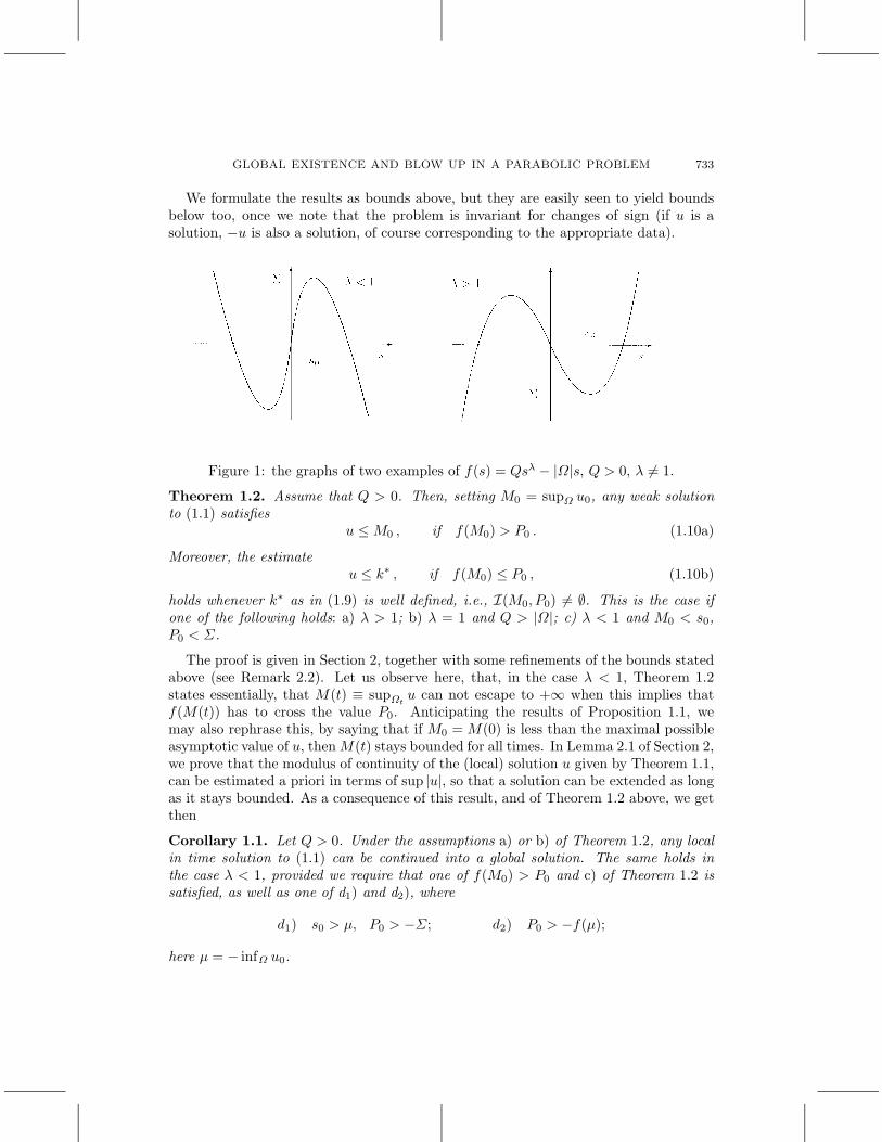
The function f is linear if � = 1; the graphs of two examples of f in the case � 6= 1,Q > 0 are sketched in Figure 1.

We also let, for any given initial datum u0,

k⇤ = inf I(M0, P0) , I(M0, P0) = {s > M0 : f(s) > P0} , (1.9)

provided I(M0, P0) 6= ;.


We formulate the results as bounds above, but they are easily seen to yield boundsbelow too, once we note that the problem is invariant for changes of sign (if u is asolution, �u is also a solution, of course corresponding to the appropriate data).

Figure 1: the graphs of two examples of f(s) = Qs� � |⌦|s, Q > 0, � 6= 1.

Theorem 1.2. Assume that Q > 0. Then, setting M0 = sup⌦ u0, any weak solutionto (1.1) satisfies

u M0 , if f(M0) > P0 . (1.10a)

Moreover, the estimateu k⇤ , if f(M0) P0 , (1.10b)

holds whenever k⇤ as in (1.9) is well defined, i.e., I(M0, P0) 6= ;. This is the case ifone of the following holds: a) � > 1; b) � = 1 and Q > |⌦|; c) � < 1 and M0 < s0,P0 < ⌃.

The proof is given in Section 2, together with some refinements of the bounds statedabove (see Remark 2.2). Let us observe here, that, in the case � < 1, Theorem 1.2states essentially, that M(t) ⌘ sup⌦t

u can not escape to +1 when this implies thatf(M(t)) has to cross the value P0. Anticipating the results of Proposition 1.1, wemay also rephrase this, by saying that if M0 = M(0) is less than the maximal possibleasymptotic value of u, then M(t) stays bounded for all times. In Lemma 2.1 of Section 2,we prove that the modulus of continuity of the (local) solution u given by Theorem 1.1,can be estimated a priori in terms of sup |u|, so that a solution can be extended as longas it stays bounded. As a consequence of this result, and of Theorem 1.2 above, we getthen

Corollary 1.1. Let Q > 0. Under the assumptions a) or b) of Theorem 1.2, any localin time solution to (1.1) can be continued into a global solution. The same holds inthe case � < 1, provided we require that one of f(M0) > P0 and c) of Theorem 1.2 issatisfied, as well as one of d1) and d2), where

d1) s0 > µ, P0 > �⌃; d2) P0 > �f(µ);

here µ = � inf⌦ u0.


(Conditions d1) or d2) are needed to bound u below.) In Section 4 we prove thefollowing results about the behaviour for large times of solutions. In the two statementsbelow we denote by u the solution found in Theorem 1.1 (more generally, u can be anyweak solution as specified in Section 4).

Proposition 1.1. Assume that b ⌘ 0, and that |u| is globally bounded by a constant.Then u(x, t) ! k uniformly in ⌦, as t !1, where k 2 R solves

Qk� � |⌦|k = P0 . (1.11)

In particular, if Q = |⌦|, � = 1, |u| can not stay bounded if P0 6= 0.

The asymptotic behaviour in Proposition 1.1 is also used to prove the next theoremon the occurrence of blow up in finite time.

Theorem 1.3. Let b ⌘ 0, Q > 0. Case � = 1 < m: Assume that Q < |⌦|, and that

either P+ ⌘ QU(0)�Z

⌦(u0)+ dx > 0 , or U(0) = max

⌦u0 , u0 6⌘ U(0) .

Then U ! +1 in finite time. The same conclusion holds in the case Q = |⌦|, m > 2,P+ > 0.

Case � < 1 m : Assume that either

i) P+ ⌘ QU�(0)�Z

⌦(u0)+ dx > ⌃ ,

or ii) U(0) = max⌦ u0, u0 6⌘ U(0) and either P0 > ⌃, or U(0) � s0. Then U ! +1in finite time.

Comparing Theorem 1.2 with Theorem 1.3, we see that our criteria for blow up orglobal boundedness of solutions are sharp in the case where U(0) = M0. In Proposi-tion 4.1 of Section 4 we give further, somewhat more refined, blow up criteria. Let usalso remark that Proposition 4.1 still holds when b 0, as well as the part of Theo-rem 1.3 independent of the assumption U(0) = M0. This follows from the argumentsin Section 4.Remark 1.1. (Examples) It is perhaps interesting to compare the results above withtwo explicit examples of blow up and global existence. As an example of blow up infinite time, consider the following well-known solution of the porous media equation.Assume m > 1, and define

u(x, t) = (1� at)�1

m�1 (1� x/L)2

m�1 ,

L = (m + 1)(m� 1)�1 , a = 2mL�1 , 0 < t < t = a�1 , 0 < x < L .

We define u in the whole domain (0, 2L) ⇥ (0, t) by an even reflection around x = L,where u = (um)x = 0. Note that u solves a problem of type (1.1), where ⌦ = (0, 2L),N = 1, aij = 1, � = 1, Q = 2 < |⌦|, @⌦ = {0, 2L}, and that u blows up at time t < 1.


Examples of global existence, di↵erent from the ones provided by constant solutions,can be constructed as follows. Assume again N = 1, aij = 1, while any value m � 1is allowed. Consider the Dirichlet problem for equation (1.1a), in an interval (�r, 0),with null boundary data, and continuous initial datum u0, with u0(0) = u0(�r) = 0.Here r > 0 is fixed arbitrarily; the solution u to the problem above is defined for allpositive times. Extend u over (�r, r), by an odd reflection across x = 0. It can be easilychecked that the extended function solves a problem of the form of (1.1), with U(t) ⌘ 0for t � 0. Note that here Q and � > 0 (besides m � 1) can be chosen arbitrarily, andthat the stability of U is due to the nonlocal character of (1.1d).

Lemma 1.1 below deals with solutions defined in an unbounded domain, but it isincluded here because we think that it sheds light on the behaviour of solutions toproblems with dynamical boundary conditions. Indeed it shows that in (a simple caseof) a domain of infinite measure, when � = 1 and m > 1, blow up may occur for anyQ > 0, as it was to be expected in view of the results above. The proof is given inSection 4.

Lemma 1.1. Consider the following problem in 1 space dimension: find T > 0, u 2L1((0,1)⇥ (0, t)) for all t < T , ut and (um)x continuous up to x = 0 for 0 t < T ,so that u solves

ut = (um)xx , x > 0 , t > 0 , (1.12a)Qut(0, t) = �(um)x(0, t) , t > 0 , (1.12b)

u(x, 0) = u0(x) , x > 0 , (1.12c)

with m > 1 and Q > 0 arbitrarily given. Assume u0 2 C2([0,1)), with u0 > 0 andu00 < 0 in [0, x0], u0(0) > sup[x0,1) u0, for a suitable x0 > 0. Moreover let (um

0 )xx(0) =�Q�1(um

0 )x(0) > 0. Then any solution u becomes unbounded (at x = 0) in finite time(and a solution exists).

A partial uniqueness result is proven in Section 5:

Theorem 1.4. Assume m = 1, � 1, aij ⌘ aij(x, t), and that kbukL1(⌦T⇥R) < 1.Then the weak solution to (1.1) is unique.

Additional comments about uniqueness can be found in Remark 5.1; see also [8]where classical solutions are considered.Remark 1.2. The methods employed here to prove local existence of solutions stillwork when condition (1.1d) is replaced with the more general

Q(U�)0(t) = A1(t)Z

@⌦� B(x, t)aij(x, t, U)(um)xi⌫j d�x + A2(t) ,

where |A1|, |B| � µ0 > 0, A1, A2 2 W 1p (0, T ), p > 1, B 2 W 1,1

1 (⌦T ). We omit thedetails for the sake of brevity.

1.i. The case of nonregular initial data. The continuity of the initial datumu0 is not essential for most of the techniques developed here. As a first instance, let


us look at the case where we merely assume u0 2 L1(⌦), and U(0) is any given realnumber. Then all the results contained in this Introduction still hold, provided wesuitably modify the notion of weak solution; i.e., we drop the requirement that u becontinuous up to t = 0, and prescribe that (1.1b) be satisfied in an L1 sense. In thissetting, M0 in (1.8) should be redefined as M0 = max(sup⌦ u0 , U(0) ); the constant T1

in Theorem 1.1 depends now on |U(0)| as well as on ku0k1,⌦.By an inspection of the proofs given below, it can be easily checked that the continuity

of u up to the initial time is not essentially used anywhere; if u0 62 C0(⌦), Lemma 2.3holds in a version yielding continuity of u only for t > 0. It is instead important tostress that the continuity of U up to t = 0 is preserved even for nonregular initial data.This follows immediately from the proof of Lemma 2.1.

The case of an initial datum u0 2 L1(⌦) can be also treated, though an essentiallydi↵erent approach is needed to prove a priori estimates for small times. The necessarytechniques are sketched in subsection 2.i below; actually the proof given in Lemma 2.4covers even the case of u0 a finite signed measure (not charging @⌦). Theorem 1.1is then a consequence of the a priori estimates, and of the approximation argumentoutlined in Section 3; obviously the existence time T1 depends now on integral normsof u0. The uniqueness result of Theorem 1.4 holds when u0 2 L1(⌦).

Many other results of this paper carry over to the case at hand. The part of Corol-lary 1.1 concerning the cases a) and b) there, stays unchanged. That is, in those cases,all the solutions can be continued for all positive times. As for Theorem 1.3, the claimsmade about the cases � = 1, Q < |⌦|, P+ > 0, and � < 1, P+ > ⌃ are proven exactlyas in Section 4 below, and the same applies to Proposition 4.1. The proof relative tothe case � = 1, Q = |⌦|, seemingly relies on u0 2 L1+p(⌦) for small p > 0, but thisassumption may be by-passed exploiting the continuity up to t = 0 of both U(t) andR

⌦ u+(t) dx, i.e., choosing as “initial time” a su�ciently small t > 0.Let us also note that even the part of Theorem 1.3 assuming U(0) = sup⌦ u0 could be

applied, at least in principle, to solutions which are not bounded as t ! 0, but such thatU(#) = sup⌦ u(·,#) for some small # > 0. A similar remark applies to Theorem 1.2.For the sake of brevity we do not dwell on these problems here.

2. A priori estimates. We start stating the following energy estimate for a solutionu to (1.1b)–(1.1d), (1.2), which is a consequence of routine calculations, at least if weassume u to be smooth, i.e., to solve the problem in a classical sense. For all p > 0 wehaveZ

⌦(t)|u|p+1 dx�

Z⌦|u0|p+1 dx + �0

ZZ⌦t

|D|u|m+p2 |2 dxd⌧

�

ZZ⌦t

�|u|p+1 + |u|p

dxd⌧ +

�(p + 1)� + p

Q�|U(t)|p+� � |U(0)|p+�

�, (2.1)

where �, �0 depend on p, m, ⇤, �, and Dv = (vx1 , . . . , vxN ). The inequality (2.1)remains in force if we replace there the absolute value |u| with the positive part u+, orwith the negative part u�. All the results below are valid for any weak solution whichalso satisfies inequality (2.1). When � = 1, this follows, for all weak solutions, via a


standard Steklov averaging procedure. Moreover, (2.1) is in force for all weak solutions,which are limits of a sequence of uniformly bounded smooth solutions of problems like(1.1b)–(1.1d), (1.2). (Note that the proof of Theorem 1.2 does not require (2.1).)

Lemma 2.1. Assume that u is a smooth solution to (1.1b)–(1.1d), (1.2). Then

|U(t)� U(✓)| �|t� ✓|�(1 + ku0kc1,⌦ + kUkc

1,(0,T )) , 0 < ✓ < t < T , (2.2)

where for � � 1, � = 1/(3�) and c = (m + �)/(2�); for 0 < � < 1, � = 1/3 andc = 1� � + (m + 1)/2. Here � > 0 depends on Q, ⇤, ⌦, N , �, T , m, but stays boundedfor bounded T .

Proof. If we let ' ⌘ 1 in (1.5), we get

Q�U�(t)� U�(✓)

�=Z

⌦(t)udx�

Z⌦(✓)

udx�Z t

✓

Z⌦

b(x, t, u) dxd⌧

⌘ I1 � I2 � I3 . (2.3)

Note that for � > 0 suitably small, say � �0(⌦), we have

|I1 � I2| �� Z

⌦{u(x, t)� u(x, ✓)}'dx

��+Z

⌦\⌦�

{|u(x, t)| + |u(x, ✓)|}(1� ') dx , (2.4)

with ⌦� = {x 2 ⌦ | d(x, @⌦) > �}, and ' 2 C1(⌦), 0 ' 1, ' ⌘ 1 in ⌦�, ' ⌘ 0in ⌦ \ ⌦�/2, |D'| �/�. From (1.5) written for this ', and from (1.3), and (2.1) withp = m, one easily derives

|I1 � I2| Z t

✓

Z⌦{|aij(um)xi'xj | + |b(x, t, u)'|}dxd⌧ + 2|⌦ \ ⌦�| kuk1,⌦T

��p

t� ✓ ��1/2 + ��

1 + kukm+µ

21,⌦T

�,

where we have set µ = max(1,�). Thus, if (t� ✓) < 1, choosing � = �0(t� ✓)1/3, andestimating I3 by means of (1.3), we recover from (2.3)

|U�(t)� U�(✓)| �|t� ✓|1/3�1 + kuk

m+µ2

1,⌦T

�. (2.5)

If (t � ✓) � 1, the same inequality follows trivially by taking � = �0. A standardapplication of the weak maximum principle allows us to estimate the sup norm appearingin the right-hand side of (2.5), i.e.,

kuk1,⌦T e⇤T (⇤T + kUk1,(0,T ) + ku0k1,⌦) . (2.6)

In the case � � 1, (2.2) follows from (2.5), (2.6), together with

|U(t)� U(✓)| = |[U�(t)]1/� � [U�(✓)]1/�| 2(��1)/�|U�(t)� U�(✓)|1/� .

The case � < 1 is treated similarly, with the help of the obvious inequality

|U(t)� U(✓)| = |[U�(t)]1/� � [U�(✓)]1/�| ��1 kUk1��1,(0,T ) |U�(t)� U�(✓)| .

Remark 2.1. The proof of Lemma 2.1 covers the case where U� in (1.1d) is replacedby a more general F (U). More exactly, we can still give an a priori continuity estimatefor U in terms of kuk1, provided the inverse function F�1 is continuous.


Lemma 2.2. Under the assumptions of Lemma 2.1, there exist two positive constants� and T0, depending on the data, such that

|U(t)| � , 0 < t < T0 , (2.7)

where, if � � m, or if Q < 0, one can take T0 = T . Moreover, if Q < 0 we have for all� > 0,

kUk1,(0,t) �1(�2 + ku0k1/�1,⌦ + |U(0)|)e�2t , 0 < t < T , (2.8)

where �2 = 0 if b ⌘ 0. If � � m and b ⌘ 0, we have

kUk1,(0,t) �1(1 + ku0k1,⌦ + |U(0)|)e�3t , 0 < t < T . (2.9)

Here �, T0, �1, �2, �3, can be given a priori as functions of the same quantities de-termining � in (2.2), but �1, �2, �3 do not depend on T , while �, T0 depend also onku0k1,⌦, |U(0)|.

Proof. Define a sequence {tn} according to

t0 = 0 , t1 = sup{t > 0 | kUk1,(0,t) < 2(|U(0)| + ku0k1,⌦) + 1} > 0 ,

tn = sup{t > tn�1 | kUk1,(0,t) < 2|U(tn�1)| + 1} > tn�1 , n > 1 ,

as long as tn < T . Elementary calculations show that,

|U(tn+1)|� |U(tn)| = 1 + |U(tn)| = 2n(1 + |U(0)| + ku0k1,⌦) , n � 1 . (2.10)

Taking into account (2.2), (2.10), we can bound below the step tn+1 � tn:

(tn+1 � tn)� � (|U(tn)| + 1)��(1 + ku0kc

1,⌦ + kUkc1,(0,tn+1)

)��1

� �02n(1�c)�1 + ku0k1,⌦ + |U(0)|

�1�c,

(2.11)

where n � 1, and �, c, � are as in Lemma (2.2). When � � m, we have c 1, sothat (2.11) yields an uniform bound below for the time step tn+1 � tn. Hence time Tis reached after a finite number of steps, and we may let T0 = T in this case. If � < mwe may just define T0 = t1.

Before treating the case Q < 0, we prove the more precise estimate (2.9). Let usremark that, if b ⌘ 0 one can let ⇤ = 0 in (2.6), and drop the double integral on theright-hand side of (2.1). Thus, an inspection of the proof of Lemma 2.1 guaranteesthat, if � � m, the term �(t � ✓)� in (2.2) can be replaced with �0(t � ✓)�0 , where �0

is independent of T , t, ✓, and �0 = 1/(3�) if (t � ✓) < 1, �0 = 1/(2�) if (t � ✓) � 1.Therefore, (2.11) gives a bound below for tn+1� tn which is independent of T , implyingthat the number n of steps needed to cover the interval (0, T ) is essentially proportionalto T . Exploiting this fact in (2.10), we find the sought-after exponential bound for|U(t)|.


Finally we turn to the case Q < 0. On letting p ! 0 in (2.1), we get

Z⌦(t)

|u|dx�Q|U�(t)| Z

⌦|u0|dx�Q|U�(0)| + �

Z t

0

Z⌦

(|u| + 1) dxd⌧ , (2.12)

where � = 0 if b ⌘ 0. Then, when Q < 0, a standard application of Gronwall’s lemmayields a global a priori estimate for ku(·, t)k1,⌦, enabling us to recover formula (2.8)from (1.6a). ⇤

Once the regularity of u at the boundary has been guaranteed by the the estimatesestablished above, our next Lemma follows via known regularity results (see [3], [15]).

Lemma 2.3. Assume that u is as in Lemma 2.1. Then there exists a continuousfunction ! : R+ ! R+, with !(0) = 0, such that

|u(x, t)� u(y, ⌧)| !(|x� y| + |t� ⌧ |) , 8(x, t) , (y, ⌧) 2 ⌦T0 ,

where T0 has been defined in Lemma 2.2, and ! depends only on Q, ⇤, ⌦, N , �, T0,m, ku0k1,⌦, and on the modulus of continuity of u0.

We give next the proof of Theorem 1.2, which is independent of the results above,and some remarks on the bounds established in the theorem.Proof of Theorem 1.2. If M(t) = sup⌦t

u attains a value M 0 larger than M0 = M(0),we may invoke the maximum principle to show that there exists a # > 0 such thatU(#) = M 0. Then, by (1.6a),

f(U(#)) = QU�(#)� |⌦|U(#) (2.13)

= QU�(0) +Z

⌦(#)(u� U(#)) dx�

Z⌦

u0 dx P0 .

Of course, if f(M0) > P0, we infer that, by continuity, U can never attain a maximumlarger than M0. If instead f(M0) P0, U can actually become larger than M0, butit must still obey the bound f(U(#)) P0, whenever U(#) = M(#). This proves thebound u k⇤, where k⇤ has been defined in (1.9). Note that k⇤ is always well definedin the cases a), b), and c) made precise in the statement. Indeed, in cases a) and b),f(s) ! +1 as s ! +1, while in case c), M0 < s0 and f(s0) = ⌃ > P0.Remark 2.2. When f(M0) P0, and k⇤ > M0, we can prove the strict inequalityu < k⇤ in ⌦t, for all t > 0, provided the aij are smooth enough (e.g., of class C2 withrespect to all their arguments), and provided k⇤ 6= 0 when m > 1. Indeed, note thatU(#) = M(#) = k⇤, for a first # > 0, would imply u(x,#) ⌘ k⇤ in ⌦, by means of (2.13).But this is a contradiction to the strong maximum principle, which does hold under theassumptions stipulated here. Indeed, reasoning by contradiction, we may assume thatu(x,#) ⌘ k⇤, so that, if m > 1, u is bounded away from 0 in ⌦⇥ (#�",#) for a suitablysmall " > 0. Therefore, the di↵erential operator in (1.1) is not degenerate even if m > 1,and the strong maximum principle is a consequence of classical parabolic theory.


As a by-product of this observation, we get that if the aij are smooth, we may allowP0 = ⌃ in case c) of Theorem 1.2. Also, if � > 1, when P0 = ⌃ and M0 < �s0, wehave u < �s0 rather than the weaker u < k⇤.

2.i. Estimates in the case of unbounded u0. In order to extend the previousanalysis to the case of unbounded initial data, we need show that an a priori L1 boundfor u at a small positive time t (to be estimated a priori too), can be given in terms ofintegral norms of u0, which is done precisely in Lemma 2.4. For subsequent times t > t,the techniques of this section apply without change (by choosing t as “initial time”).Let us denote in the following

R(�) = ku0k1,⌦\⌦�, 0 < � < �0 ,

where ⌦� and �0 have been defined in the proof of Lemma 2.1. Of course R(�) ! 0 as� ! 0.

Lemma 2.4. Let u be as in Lemma 2.1. Then, a t > 0 can be determined a prioriin terms of R, ku0k1,⌦ and U(0), so that kUk1,(0,t), ku(·, t )k1,⌦ and the modulus ofcontinuity of U over [0, t ] can be estimated a priori in terms of the same quantities.

Proof. We begin as in the proof of Lemma 2.1, but a di↵erent approach is needed totreat the second integral in (2.4). To this end we find by standard integration by partsZ

⌦(t)(|u|� Y (t))+(1� ') dx

Z

⌦(|u0|� Y (t))+(1� ') dx + �

ZZ⌦t

[|aij(um)xi'xj | + |b|(1� ')] dxd⌧ ,

where we denote Y (t) = kUk1,(0,t) + 1, and ' is the same testing function as in (2.4).It followsZ

⌦\⌦�

|u(x, t)|(1� ') dx Z

⌦\⌦�

|u0|dx + ��Y (t) + �

ZZ⌦t

|aij(um)xi'xj |dxd⌧

+ �

ZZ⌦t

|b|dxd⌧ ⌘ J1 + J2 + J3 + J4 .

In order to bound J3, J4 we can use here neither the energy inequality (2.1), nor themaximum principle. Instead we employ the following estimates, which can be provenas in [1], looking at u as at the solution of a standard Dirichlet problem. Let

t

�2kukm�1

1,⌦t 1 (2.14)

(� will be chosen later as a function of t). Then, setting w = max(u, 1), and W (t) =sup0<⌧<t kw(·, ⌧)k1,⌦, we have

|u(x, t)| �t�N/(N(m�1)+2)W (t)2/(N(m�1)+2) + Y (t) , x 2 ⌦, (2.15)Z t

0

Z⌦�

|Dum|p dx⌧ �t↵{W (t)� + Y (t)�} , (2.16)


for certain positive ↵, �, � = ↵, �, �(N,m, p), and p 2 (1, (Nm + 2)/(Nm + 1)). Belowwe still denote by ↵, �, �, various positive constants depending on N , m, p.

By means of the bounds above, we readily arrive at

J3 �t↵��1/p{W (t)� + Y (t)�} , J4 �tW (t) .

With the help of this remark, we get, reasoning as in Lemma 2.1,

|U�(t)� U�(0)| �t↵��1/p{W (t)� + Y (t)�} + �R(�) + ��Y (t) ;

choosing � = t", with p↵ > " > 0 to be fixed later, we find therefore an estimate of themodulus of continuity of U at t = 0, depending on R, W (t), and on kUk1,(0,t). In turn,ku(·, t)k1,⌦ can be bounded in terms of kUk1,(0,t), as in (2.12). Finally, a small t > 0such that

kUk1,(0,t) �(U(0), ku0k1,⌦) , 0 < t < t ,

can be found following the ideas in the proof of Lemma 2.2. For 0 < t < t, u(·, t)satisfies the L1 estimate (2.15), provided we show that t satisfies (2.14), for � chosenas above. But this is certainly implied by

t1�2"� N(m�1)N(m�1)+2 �(U(0), ku0k1,⌦) 1/2 , 0 < " <

�N(m� 1) + 2

��1,

which simply amounts to a possible redefinition of ", t (we stress the fact that the choiceof t can be performed a priori; i.e., it only depends on the initial data). The proof isconcluded by noting that the modulus of continuity of U , which we have estimated att = 0, can be estimated a priori at each t belonging to, say, (0, t/2] by means of themethods applied in Lemma 2.1. Indeed, for each such t, u is bounded over [t/2, t ].

3. Proof of the existence results. We begin with the proof of Theorem 1.1; someauxiliary results, needed in the proof, are postponed to a second subsection. The sectionis closed by some additional existence results which we think are of some interest.

3.i. Proof of Theorem 1.1. The proof will be achieved through approximation by asequence of smoothed problems. Fix an extension operator, mapping any v 2 H", "

2 (⌦T )to a continuous function defined in RN+1, and preserving the norm in the space H", "

2 .We use here the notation of [13]. Denote again by v the extension of the original function.Then set jn(v) = v ⇤ Jn, where {Jn} is a given sequence of standard mollifying kernelsin RN+1. Fix � > 0 and let

aij(x, t, v) = aij(x, t, v)m(|v| + �)m�1 ;

we also define anij and bn to be suitably smooth approximations of aij , b. We may

assume that the structure assumptions stated in Theorem 1.1 are fulfilled uniformly inn by an

ij , bn. In fact in all the arguments below, the anij can be assumed to be globally


bounded; indeed, the sup norms of the functions replacing v in anij can be estimated a

priori (owing to the choice of the function hn in (3.1c)). We look at the problem

ut =�an

ij(x, t, jn(u))uxi

�xj

+ bn(x, t, u) , in ⌦T , (3.1a)

u(x, 0) = u0n(x) , x 2 ⌦ , (3.1b)

u(x, t) = hn� 1Q

Z t

0

Z@⌦� an

ij(⇠, ⌧, jn(u)(⇠, ⌧))u⇠i⌫j d�⇠ d⌧ + (hn)�1(U(0))�, on ST , (3.1c)

where u0n and, respectively, hn 2 C1(R) \ L1(R), are smooth approximations of u0

and, respectively, of h(s) = min(n,max(�n, s1/�)) (if m > 1 we replace n with 1/� inthe definition of h ). We may also assume that the second-order compatibility conditionsat @⌦ ⇥ {0} are satisfied for (3.1).

Equation (3.1a) can be put in a nondivergence form, so that we may still apply theproof of Lemma 3.1 below to get local existence for (3.1). In order to extend the lifespan of the solution up to t = T , we note that, for n fixed, the global boundedness of thesolution and the a priori estimates needed in Lemma 3.2 follow from the weak maximumprinciple and from the definition of jn. Thus, the proof given there covers the case athand, thereby implying the existence of a global solution un to (3.1). Indeed, the termcontaining jn(un)xj u

nxi

in (3.1a) can be regarded as a term vi,nunxi

, with smooth vi,n.If m = 1, the existence of a weak solution to the original problem (1.1) follows from

a standard procedure of integration by parts in (3.1a), and on letting n ! 1 in theresulting integral equality. In the limiting process we exploit the a priori estimatesof Section 2, which hold for each un, independently of n. That is, we use the uniformcontinuity given by Lemma 2.3, and the L2 bounds for Dun, implied by (2.1). Therefore,the solution is defined only in the time interval (0, T0), with T0 given in Lemma 2.2.

If m > 1, we first take the limit n ! 1; note that kunk1,⌦T �(�) for all n,

due to the definition of hn. Hence, as we remarked above when dealing with the casem = 1, {un} is equicontinuous and {|Dun|} is bounded in L2(⌦T ) (such estimatesdepend, in principle, on �). We may assume that un ! u�, where u� solves a problemsimilar to (3.1); note however that, on letting n !1, we got rid of the approximationby convolution. Then, we are able to apply to u� the estimates given above for thedegenerate case m > 1, which are therefore independent of � > 0. The proof is completedby letting � ! 0.Remark 3.1. If U(0) = sup⌦ u0 and Q > 0, we may assume that U(0) = sup⌦ u0n,U 0n(0) > 0, where Un = un

|ST. Thus, an application of the strong maximum principle

yields that Un is increasing in time, provided bn 0, for all n. Therefore, in this case,the limit solution u to (1.1) is such that U = u|ST

is nondecreasing in time.

3.ii. Auxiliary results. Let us consider the problem

ut = aij(x, t, u,Du)uxixj + b(x, t, u,Du) , in ⌦T , (3.2a)u(x, 0) = u0(x) , x 2 ⌦ , (3.2b)


u(x, t) = h�Z t

0

Z@⌦� c(⇠, ⌧, u(⇠, ⌧),Du(⇠, ⌧)) d�⇠ d⌧

�+ F (x, t) , on ST , (3.2c)

where we assume that for ⇤ > 1, ↵ 2 (0, 1) given, and for all compact sets K ⇢ RN+1,

kaij(·, ·, u,p)kH↵, ↵

2 (⌦T ) �(K), 8(u,p) 2 K ,

��@aij

@u

��+ ��@aij

@pk

�� ⇤, in ⌦T ⇥RN+1,

and b and c fulfill similar requirements;

aij(x, t, u,p)pipj � ⇤�1|p|2 , 8(x, t) 2 ⌦T , u 2 R , p = (pi) 2 RN ;

F 2 H2+↵, 2+↵2 (⌦T ) , h 2 C2(R) , kh0k1,R < 1 , u0 2 H2+↵(⌦) ;

the obvious compatibility conditions (of order 2) are satisfied at @⌦ ⇥ {t = 0} .

Lemma 3.1. Under the assumptions above, problem (3.2) admits a unique solutionu 2 H2+↵, 2+↵

2 (⌦T1), for a suitably small T1 > 0.

Proof. Define

X = {u 2 H1+↵, 1+↵2 (⌦T ) : kuk

H1+↵, 1+↵2 (⌦T )

M ,u(x, 0) = u0(x) , x 2 ⌦} .

The solution will be found as a fixed point of the mapping T : X ! X defined as follows.Pick v 2 X and define T (v) = v, where v solves the standard linear problem obtainedfrom (3.2) by replacing u, Du with v, Dv in the arguments of aij , b, c. It follows fromclassical estimates ([13], Theorem 10.1, Chapter IV) that

kvkH2+↵, 2+↵

2 (⌦T ) �(M) ,

whencekvk

H1+↵, 1+↵2 (⌦T )

�0 + �1T↵/2 ,

where �1 depends on M , while �0 depends only on the (2+↵) norm of u0. Therefore wehave v 2 X for M , T suitably chosen. Then choose q > N+2 such that ↵ < 1�(N+2)/q.Let vi 2 X, vi = T (vi), i = 1, 2, V = v1�v2, V = v1�v2. It follows from the embeddingin [13], Lemma 3.3, Chapter II, and from classical solvability results (ibid., Theorem. 9.1,Chapter IV), that

��V ��H1+↵, 1+↵

2 (⌦T ) �

� ��V ��W 2,1

q (⌦T )+��V (·, 0)

��W 2�2/q

q (⌦)

� �0

�kV k1,⌦T

+ kDV k1,⌦T

� �0T↵/2 kV k

H1+↵, 1+↵2 (⌦T )

,

where the constants denoted by �, �0 depend on the data but are stable as T ! 0(see also Appendix 2 of [8]); the constants �0 also depend on M . It follows that T iscontractive for small T . Then T has one fixed point u 2 X; i.e., u is the solution to theproblem at hand.


Lemma 3.2. Under the same assumptions of Lemma 3.1, the solution u found therecan be extended to a global solution defined in ⌦T , if we assume that the modulus ofcontinuity of aij(·, ·, u(·, ·),Du(·, ·)) is estimated a priori over ⌦T .

Proof. Let y(t) = kuk1,⌦t+ kDuk1,⌦t

. Using the assumptions stipulated at thebeginning of this subsection, and in the statement, together with the estimates quotedabove, we get for q as in the proof of Lemma 3.1,

y(t) ��kukW 2,1

q (⌦t)+ ku0kW 2�2/q

q (⌦)

�

��1 + kbkq,⌦t

+ kckq,@⌦⇥(0,t)

� �

�1 +

Z t

0y(⌧)q d⌧

�1/q,

where � is bounded over (0, T ). Gronwall’s lemma yields an a priori bound for y(t),and therefore a bound for kukW 2,1

q (⌦t)+ ku0kW 2�2/q

q (⌦). Exploiting those bounds, the

embedding result and the a priori estimates quoted in the proof of Lemma 3.1, we finda bound for kuk

H2+↵, 2+↵2 (⌦t)

which is essentially independent of t 2 (0, T ). The proofis completed by noting that the existence time T1 given in Lemma 3.1 depends only onthe (2 + ↵) norm of the initial datum, so that, finally, the whole interval (0, T ) can becovered by a finite number of steps of the same length T1.Remark 3.2. It is clear that the a priori estimates of Lemma 3.2 require for h onlythat h 2 W 1

1(R), so that classical existence results for such h can also be proven, byapproximating h with smooth functions. Of course in this case the first space derivativesof the solution, but not the second ones, in general, are continuous up to ST .

This remark applies to problems with a change of phase taking place in @⌦, whenU� in (1.1d) is replaced with F (U) 2 U + H(U), H being the Heaviside graph; indeed,|F (U1)� F (U2)| � |U1 � U2|, U1, U2 2 R.

3.iii. Additional classical existence results. We sketch here an approach yield-ing, in some cases, a priori estimates implying the existence of classical solutions (i.e.,solutions of class H2+↵, 2+↵

2 (⌦T )). We assume in this subsection that m = 1, butthe case m > 1 can be treated similarly when u is bounded away from u = 0. Ifaij(x, t, u) = a(x, t, u), i, j = 1, . . . , N (e.g., in any case if N = 1), and � = 1, weemploy Kircho↵’s transform to rewrite equation (1.2) as follows:

vt = a(x, t, u)� v + F (x, t, u,Dv) , v(x, t) =Z u(x,t)

0a(x, t, ⌘) d⌘ .

Besides stipulating the assumptions listed in subsection 3.ii, we understand that a hasthe extra regularity required by the method sketched here. On the other hand, we maylet b in (1.2) depend on Du, as far as it is globally Lipschitz continuous in Du; it is easyto check that the a priori estimates of Section 2 cover this case. Then the function Fabove is smooth, and grows at most linearly in Dv. Condition (1.1c)–(1.1d) transformsto

vt(x, t) = Q�1a(x, t, U)Z

@⌦� @v

@⌫d� + g(x, t, U) , (3.3)


for a suitable g. The techniques of Lemma 3.2 give the sought-after classical globalestimates, if we keep in mind that the Holder norm of U is a priori bounded by Lem-mata 2.1, 2.2. In this connection, note that when h(s) ⌘ s, s 2 R, as in the case athand, c in (3.2c) can contain a multiplicative factor c1(x, ⌧).

If � < 1 a similar method can be used over any time interval where we know a priorithat u is bounded (see Section 2). In this case (3.3) keeps the same structure: we onlyneed replace the factor a on the right-hand side with ��1u1��a. If � > 1 the samearguments still hold, provided U is bounded away from U = 0.

If aij = aij(x, t) are smooth, one can prove classical existence applying directly themethods of subsection 3.ii when � = 1; when � 6= 1 we may take the nonlinear termu��1 to the right-hand side of (1.1d), reasoning as above.

4. Proof of the results about blow up or asymptotic behaviour. In thisSection, we denote by u a solution which is approximated by smooth solutions, as insubsection 3.i. (More generally, u can be any weak solution satisfying the energy in-equality (2.1), and the monotonic behaviour of Remark 3.1, when the latter applies; seealso the remarks following (2.1); a slight generalization of (2.1) is required in Proposi-tion 4.1, when � < 1.) We begin by establishing the behaviour at infinity of solutionswhich stay bounded for all times.Proof of Proposition 1.1. If u is globally bounded, it is also uniformly continuousby virtue of Lemma 2.1. Moreover, (2.1) makes sure that

Z +1

0

Z⌦|Dum|2 dxd⌧ < 1 . (4.1)

Assume that k is a constant such that U(tn) ! k for a suitable sequence tn ! 1,and fix arbitrarily " > 0. Owing to the already-recalled uniform continuity, there exist� = �(") > 0 and n" 2 N, such that |U(t) � k| " for |t � tn| �, for all n > n".Because of (4.1), there exists also a sequence {t0n}, |tn � t0n| �, such that

kum(·, t0n)� Um(t0n)k22,⌦ � kDum(·, t0n)k22,⌦ ! 0 , as n !1 ,

where we have also used Poincare’s inequality. Thus, perhaps extracting a subsequence,which we still denote by {t0n}, we have

��P0 �Qk� + |⌦|k�� = lim

n!1

��Q(U�(t0n)� k�)�Z

⌦(t0n)(u� k) dx

�� (k,Q, |⌦|)(" + "�).

On letting " ! 0, we have that k satisfies (1.11). In the cases where such a constant isnot uniquely determined, we remark that U(t) can not oscillate between two such valuesanyway, because it would attain all the intermediate values infinitely many times, whichis precisely what we have ruled out above. Therefore we have

lim supt!1

U(t) = lim inft!1

U(t) = k , k as in (1.11) .


The uniform convergence u(x, t) ! k in ⌦ as t ! 1 follows essentially from thearguments above: If u does not converge to k, the uniform continuity implies that|u� k| > " in a sequence of sets Dn = {|x� xn| < "}⇥ (⌧n, ⌧n + "), Dn ⇢ ⌦ ⇥ (0,1),for a small but fixed " > 0. This leads us to an inconsistency, because on one hand,kum � Umk2L2(⌦⇥R+) is finite, owing to (4.1) and to Poincare’s inequality. On the otherhand, the same quantity is minorized by the divergent series �"

Pn |Dn|, where �" > 0

is a suitable positive constant. ⇤The following result is the main tool used in the proofs collected in this section.

Lemma 4.1. Assume that b ⌘ 0, Q > 0, � < m, and that for some t0 > 0, we have

U(t) � � > 0 , for all t � t0 , (4.2)|E(t)| � ⌘ > 0 , for all t � t0 , E(t) = {x 2 ⌦ : u(x, t) �U(t)} , (4.3)

for �, ⌘ and � 2 (0, 1) given. Then u becomes unbounded in a finite time.

Proof. Let w = Uq � uq+, for t � t0, and a fixed q > 0. Since w = 0 on @⌦, we get

from Poincare’s inequality

�

Z⌦(t)

|Dw|2 dx �Z

⌦(t)|w|2 dx �

ZE(t)

|w|2 dx � ⌘(1� �q)2U(t)2q .

Then, from (2.1), we get for q = (m + p)/2, p > 0,

U(t)�+p � U(t0)�+p � � + p

Q(�p + �)

Z⌦(t0)

up+1+ dx + �0

Z t

t0

Z⌦|Du

m+p2

+ |2 dxd⌧

� C + �0

Z t

t0

U(⌧)m+p d⌧ ,

where C 2 R depends on u(·, t0). Assume that u does not become unbounded in finitetime. Then, using the bound below U(t) � �, we have, after a su�ciently long timet1 � t0 has elapsed,

U(t)�+p � C0 + �0

Z t

t1

U(⌧)m+p d⌧ , t � t1 ,

with C0 > 0. Taking into account that � < m, it is now a trivial matter to show thatU must blow up in finite time. Indeed U(t)�+p � y(t), where y solves

(y0 = �0 y

m+p�+p , t > t1 , m+p

�+p > 1 ,

y(t1) = C0 .

Proof of Theorem 1.3. 1) Assume that � = 1, Q < |⌦|, and U(0) = maxu0,u0 6⌘ U(0). As noted in Remark 3.1, u is such that U(t) is nondecreasing in time. Let


Tmax 1 be the maximal existence time for u. If U(t) ! U1 < 1 as t ! Tmax, themonotonicity of U is contradicted, because by virtue of Proposition 1.1 we have

U1 =P0

Q� |⌦| = U(0) +|⌦|U(0)�

R⌦ u0 dx

Q� |⌦| < U(0) .

Thus U(t) ! +1 as t ! Tmax, and (4.2) is satisfied. To be able to apply Lemma 4.1above, we have to check that (4.3) is also fulfilled. Indeed, defining H�(t) = {x 2 ⌦ |u(x, t) > �U(t)}, with � 2 (0, 1) fixed, we have for large t,

QU(t) � QU(0)+ �Z

⌦(u0)+ dx +

Z⌦(t)

u+ dx � C + �U(t)|H�(t)| , (4.4)

where C is a constant depending on u0, U(0). Note that the first inequality in (4.4) is avariant of (2.1), which can be obtained by letting p ! 0 in the version of (2.1) writtenwith the positive part u+ replacing |u|. Thus, for a suitable ⌘ > 0, and provided1 > � > Q/|⌦|, (4.4) yields

|H�(t)| Q��1 � C��1U�1(t) |⌦|� ⌘ , t � t0 ,

where t0 is large enough. Of course (4.3) follows at once.2) Assume that � < 1, and U(0) = maxu0, u0 6⌘ U(0). We also stipulate, as

in the statement, that either i) P0 > ⌃, or ii) U(0) � s0 (the quantities s0 and ⌃have been defined in (1.8)). As above, we may assume that U(t) ! U1 1 fort ! Tmax. If U1 < 1, we have both P0 = QU�

1 � |⌦|U1, with U1 � U(0), andP0 > QU(0)� � |⌦|U(0), owing to the assumption U(0) 6⌘ u0. This is seen to beimpossible, by a quick glance at the behaviour of the function f(s) = Qs� � |⌦|s,displayed in the Introduction, both in case i) and in case ii). Therefore, U(t) ! +1 ast ! Tmax. In order to show that (4.3) also holds, we reason as in the first step of theproof: for large t,

QU�(t) � QU�(0)+ �Z

⌦(u0)+ dx +

Z⌦(t)

u+ dx � C + �U(t)|H�(t)| ,

whence|H�(t)| QU��1(t)��1 � C��1U�1(t) ! 0 , t ! Tmax

(note that here � 2 (0, 1) can be chosen arbitrarily).3) Let � = 1, Q < |⌦|, and P+ ⌘ QU(0) �

R(u0)+ > 0. This case actually follows

from Proposition 4.1 with ⇢ = 0 there, but we give here a simple direct proof. From(4.4) we get U(t) � P+/Q > 0, t � 0. We also find as in the first part, but nowexploiting the positivity of P+,

|H�(t)| Q��1 � P+��1U�1(t) < Q��1 < |⌦| ,

if 1 > � > Q/|⌦|. Then the assumptions of Lemma 4.1 are satisfied, and u blows up infinite time.


4) Let � < 1, and P+ ⌘ QU�(0) �R(u0)+ > ⌃. The bound below U(t) �

(P+/Q)1/� > 0 can be proven as in part 3) of this proof, as well as the first inequalityin

|H�(t)| QU��1(t)��1 � P+��1U�1(t) |⌦|� ⌘ .

The latter inequality is instead equivalent to

QU�(t)� �(|⌦|� ⌘)U(t) P+ . (4.5)

In turn, due to the assumption P+ > ⌃, (4.5) holds for any value U(t) > 0, provided1� � > 0 and ⌘ > 0 are chosen small enough.

5) Let � = 1, |⌦| = Q, P+ > 0, m > 2. In this case, one can easily show that|H�(t)|! |⌦| at blow up. Then we have to resort to the following alternative method,requiring the restriction m > 2. Set

�p(t) = |⌦|U1+p+ (t)�

Z⌦(t)

u1+p+ dx ,

for t � 0, p > 0. Then, we get from (2.1) and from Poincare’s inequality,

�p(t)� �p(0) � �0

Z t

0

Z⌦|Du

m+p2

+ |2 dxd⌧ � �0

Z t

0

Z⌦|D[u

m+p2

+ � Um+p

2+ ]|2 dxd⌧

� �0

Z t

0

Z⌦|u

m+p2

+ � Um+p

2+ |2 dxd⌧ � �0

Z t

0

Z⌦|u1+p

+ � U1+p+ |

m+p1+p dxd⌧

� �0

Z t

0

��Z

⌦(U1+p

+ � u1+p+ ) dx

��m+p1+p

d⌧ � �0

Z t

0�

m+p1+p

p (⌧) d⌧ , (4.6)

where we have made use of the elementary fact |a� b|� |a�� b�|, for � = (m+p)/(2+2p) > 1. Note that the last inequality is satisfied for p > 0 suitably small, due to theassumption m > 2. Formula (4.6) immediately implies blow up in finite time, provided�p(0) > 0, which can be guaranteed again by choosing p close enough to 0, because�p(0) ! P+ when p ! 0. ⇤

Our next result implies blow up of solutions under di↵erent, and in some casessharper, conditions than the ones given in Theorem 1.3. For example, consider a prob-lem with Q < |⌦|, � = 1 < m, and initial data u0, U(0), with

u0(x) = a > U(0) > 0 , in ⌦1 ⇢ ⌦ , u0(x) = b 2 (0, U(0)) , in ⌦ \ ⌦1

(such discontinuous initial data are admissible,; see subsection 1.i). Proposition 4.1below allows us to prove blow up under the assumption

(Q� |⌦1|)(U(0)� b) > |⌦1|(a� U(0)) ,

rather than under the stronger P+ > 0, as we did in Theorem 1.3.


Proposition 4.1. Assume that b ⌘ 0, Q > 0, and that for some 0 ⇢ < 1,

K(⇢) ⌘ QU�(0)(1� ⇢�)�Z

⌦(u0 � ⇢U(0))+ dx > 0 ;

assume moreover that either � = 1 < m and Q < |⌦|, or � < 1 and ⇢U(0) > s0. Thenconditions (4.2), (4.3) are fulfilled, and therefore u becomes unbounded in finite time.

Proof. By arguments exploited several times in this paper (see e.g., part 1) of the proofof Theorem 1.3), we prove

QU�(t) � QU�(0)�Z

⌦(u0 � ⇢U(0))+ dx +

Z⌦(t)

(u� ⇢U(0))+ dx , (4.7)

for all t > 0 such that U(⌧) � ⇢U(0) for 0 < ⌧ < t. On the other hand, for all such twe have by the same token

U(t) � (A(⇢)/Q)1/� , (4.8)

withA(⇢) = QU�(0)�

Z⌦

(u0 � ⇢U(0))+ dx .

By assumption A(⇢) > Q⇢�U�(0), so that (4.8) actually implies that (4.7) holds for allt > 0. More exactly we have

U(t) ��⇢�U�(0) + Q�1K(⇢)

�1/�, t > 0 , (4.9)

so that (4.2) is satisfied.Note that (4.9) implies �U(t) > ⇢U(0) if 1� � > 0 is small enough. For such �, and

H�(t) as in the proof of Theorem 1.3, we infer from (4.7),

QU�(t) � A(⇢) + (�U(t)� ⇢U(0))|H�(t)| ,

whence |H�(t)| |⌦|� ⌘, for ⌘ > 0, if

QU�(t)�A(⇢) (|⌦|� ⌘)(�U(t)� ⇢U(0)) . (4.10)

Hence we discriminate between the cases � = 1 and � < 1. If the former holds, (4.10)is equivalent to

U(t)��(|⌦|� ⌘)�Q

�� ⇢(|⌦|� ⌘)U(0)�A(⇢) . (4.11)

Next we choose � and ⌘ suitably, so that 1 > � > Q/(|⌦|� ⌘). Then (4.11) is implied,recalling (4.9), by

�⇢U(0) + Q�1K(⇢)

��(|⌦|� ⌘)�Q

�� ⇢(|⌦|� ⌘)U(0)�A(⇢) .


This last inequality reduces to

�K(⇢) � (1� �)Q⇢U(0) ,

which certainly holds if � is chosen close enough to 1; this can be done safely once ⌘has been fixed small enough.

Finally, let us prove condition (4.3) also when � < 1. Let us define

g(s) = Qs� � �(|⌦|� ⌘)s , s > 0 ,

where � and ⌘ are to be chosen. By elementary calculations we see that (4.10) can beput in the form

g(U(t)) g(⇢U(0)) + K(⇢)� (1� �)(|⌦|� ⌘)⇢U(0) . (4.12)

Since K(⇢) > 0 by assumption, we only need show g(U(t)) g(⇢U(0)), provided 1� �is suitably small. To this end, we recall that we have stipulated ⇢U(0) > s0; moreover,obviously, g0(s) ! f 0(s) as � ! 1, ⌘ ! 0, where f has been defined in the Introduction.Thus we may assume, after choosing suitable � and ⌘, that g0(s) < 0 for s > ⇢U(0) > s0.But then U(t), owing to (4.9), belongs to the domain where g is decreasing and lessthan g(⇢U(0)), so that (4.12) holds and the proof is concluded.Proof of Lemma 1.1. Assume that u as in the statement is given. Let us considerthe function

v(x, t) = U(t)(�e�"x + 1� �) , x � 0 , t � 0 ,

where U(t) = u(0, t), and �, " > 0 are to be chosen presently. It can be seen byelementary calculations that

v(x, 0) � u0(x) , x � 0 ,

for all " < "0, and "0, � 2 (0, 1) suitably fixed. We also have

vt � (vm)xx � (1� �)U 0(t)�m2�"2Um(t) � 0 ,

provided"2 (1� �)U 0(t)

�m2�Um(t)

��1, (4.13)

which holds in a maximal time interval [0, t1]; note that t1 > 0, if " is small enough (sothat (4.13) is strictly satisfied for t = 0). By a standard comparison argument, we havev � u in (0,1)⇥ (0, t1); on the other hand v = u at x = 0, so that

ux(0, t) vx(0, t) = �"�U(t) , 0 < t < t1 .

HenceU 0(t) � Q�1m"�Um(t) , 0 < t < t1 , (4.14)


implying that U blows up at a finite time T , unless t1 < T . But in this case, (4.13)holds with an equality sign at t = t1, so that, also by means of (4.14), we get

"2 = (1� �)U 0(t1)�m2�Um(t1)

��1 � (1� �)"(mQ)�1 .

Finally, the last inequality can be ruled out simply by choosing " < (1� �)(mQ)�1.The existence of a solution to (1.12) is actually a consequence of other results given

here, despite the fact that the domain is unbounded. Indeed, let us denote by zr asolution to the problem posed for (1.12a) in x 2 (0, 2r), r > 0, with initial and boundarydata, of the type of (1.1b)–(1.1d),

2QZ0r(t) = �(zrm)x(0, t) + (zr

m)x(2r, t) , Zr(t) = zr(0, t) = zr(2r, t) ,

zr(x, 0) = u0(x) , 0 < x < r , zr(x, 0) = u0(2r � x) , r < x < 2r .

It is easy to see that the methods in Section 2 give a local modulus of continuity for zr

which is independent of r, so that the existence time T0 of Lemma 2.2 can be assumed tobe independent of r too. Then a solution u is found as the limit of a suitable subsequenceof {zr} as r ! 1. The smoothness of u up to x = 0 follows from the arguments insubsection 3.iii. This concludes the proof.

5. Proof of Theorem 1.4. Let u1, u2 be two weak solutions of the same problem(1.1). Under the assumptions of Theorem 1.4, it follows from standard calculations thatfor 0 < t < T ,

ku1 � u2k1,⌦t ��(t) , �(t) = kU1 � U2k1,(0,t) .

Then, for the same function ' used in the proof of Lemma 2.1, we have

QU�1 (t)�QU�

2 (t) =Z

⌦(t)(u1 � u2)(1� ') dx +

Z⌦(t)

(u1 � u2)'dx

�ZZ

⌦t

�b(x, t, u1)� b(x, t, u2)

�dx⌧ (5.1)

��(t) + �t�(t) +��Z

⌦(t)(u1 � u2)'dx

�� .

The last term in (5.1) can be bounded with �t��1�(t), by means of calculations involv-ing cuto↵ functions of the type of ', similarly to what we did in the proof of Lemma 2.1.

We also use the obvious fact

|U�1 (t)� U�

2 (t)| � ��max(kU1k1 , kU2k1)

��1|U1(t)� U2(t)| .

Putting this information into (5.1) we get

�0�(t) ��(t) + t��1�(t) .


Then, taking � = �0/2 and then t = t(�0) > 0 suitably small, we may absorb both thefirst and the second term on the right-hand side into the left-hand side; of course thisimplies that �(t) ⌘ 0.Remark 5.1. The proof given above works even in the case � > 1, at least as long asU(t) 6= 0. More generally, it covers the case where U� is replaced with F (U), providedthe inverse function F�1 is Lipschitz continuous. This also applies to problems with achange of phase taking place in @⌦; see Remark 3.2.

REFERENCES

[1] D. Andreucci and E. DiBenedetto, A new approach to initial traces in nonlinear filtration,Annales Inst. H. Poincare, Anal. Non Lineaire, 7 (1990), 305–334.

[2] P. Colli and J.F. Rodrigues, Di↵usion through thin layers with high specific heat , AsymptoticAnal., 3 (1990), 249–263.

[3] E. DiBenedetto, Continuity of weak solutions to a general porous medium equation, IndianaUniv. Math. J., 32 (1983), 83–118.

[4] M.T. Dzhenaliev, Solvability of boundary value problems for loaded linear equations with irregularcoe�cients, Di↵. Uravn., 27 (1991), 1585–1595.

[5] J. Escher, Quasilinear parabolic systems with dynamical boundary conditions, Comm. P.D.E.,18 (1993), 1309–1364.

[6] J. Escher, On quasilinear fully parabolic boundary value problems, Di↵. Integral Eqs., 7 (1994),1325–1343.

[7] J. Escher, On the qualitative behaviour of some semilinear parabolic problems, Di↵. IntegralEqs., 8 (1995), 247–267.

[8] R. Gianni, Global existence of a classical solution for a large class of free boundary problems inone space dimension, Nonlinear Di↵. Eqns. Appl., 2 (1995), 291–321.

[9] K. Groger, Initial boundary value problems from semiconductor device theory, Zeitschrift Angew.Math. Mech., 67 (1987), 345–355.

[10] L.I. Kamynin, Solution of the fifth boundary value problem for a second order parabolic equationin a non-cylindrical region, Sibirski Mat. Zh., 9 (1968), 1153–1166.

[11] L.I. Kamynin, Applications of parabolic potentials to boundary value problems of mathematicalphysics II , Di↵. Eqns., 27 (1991), 441–453.

[12] M. Kirane, Blow-up for some equations with semilinear dynamical boundary conditions of par-abolic and hyperbolic type, Hokkaido Math. Jour., 21 (1992), 221–229.

[13] O.A. Ladyzenskaja, V.A. Solonnikov, N.N. Ural’tzeva, “Linear and Quasilinear Equations ofParabolic Type,” Transl. of Math. Mon. Providence, R.I. AMS, 23 (1968).

[14] E. Magenes, Some new results on a Stefan problem in a concentrated capacity, Atti Acc. Naz.Lincei Classe Sci. Fis. Mat. Nat. (9) Mat. Appl., 3 (1992), 23–34.

[15] M.M. Porzio, V.Vespri, Holder estimates for local solutions of some doubly nonlinear degenerateparabolic equation, J. Di↵. Eqns., 103 (1993), 146–178.

[16] R.E. Showalter, Degenerate evolution equations and applications, Indiana Univ. Math. Jour., 23(1974) 655–677.

[17] A. Tikhonov, On boundary conditions containing derivatives of order higher than the order ofthe equation, Mat. Sbornik, 26 (1950), 35–56; Transl. in Translations of AMS Series 1 Di↵. Eqns.,4, 440–466.

[18] M. Ughi, Teoremi di esistenza per problemi al contorno di quarto e quinto tipo per un’equazioneparabolica lineare, Riv. Mat. Univ. Parma, 5 (1979), 591–606.

global existence and blow up in a parabolic problem with ...

Documents