GLOBAL DYNAMICS OF DISCRETE MONOTONE MAPS IN THE …

University of Rhode Island University of Rhode Island

DigitalCommons@URI DigitalCommons@URI

Open Access Dissertations

2019

GLOBAL DYNAMICS OF DISCRETE MONOTONE MAPS IN THE GLOBAL DYNAMICS OF DISCRETE MONOTONE MAPS IN THE

PLANE AND IN RPLANE AND IN RN

James Marcotte University of Rhode Island, [email protected]

Follow this and additional works at: https://digitalcommons.uri.edu/oa_diss

Recommended Citation Recommended Citation

Marcotte, James, "GLOBAL DYNAMICS OF DISCRETE MONOTONE MAPS IN THE PLANE AND IN RN" (2019). Open Access Dissertations. Paper 1101. https://digitalcommons.uri.edu/oa_diss/1101

This Dissertation is brought to you for free and open access by DigitalCommons@URI. It has been accepted for inclusion in Open Access Dissertations by an authorized administrator of DigitalCommons@URI. For more information, please contact [email protected].

GLOBAL DYNAMICS OF DISCRETE MONOTONE MAPS IN THE PLANE

AND IN RN

BY

JAMES MARCOTTE

A DISSERTATION SUBMITTED IN PARTIAL FULFILLMENT OF THE

REQUIREMENTS FOR THE DEGREE OF

DOCTOR OF PHILOSOPHY

IN

MATHEMATICS

UNIVERSITY OF RHODE ISLAND

2019

DOCTOR OF PHILOSOPHY DISSERTATION

OF

JAMES MARCOTTE

APPROVED:

Dissertation Committee:

Major Professor Orlando Merino

Mustafa Kulenovic

Araceli Bonifant

Richard Vaccaro

Nasser H. Zawia

DEAN OF THE GRADUATE SCHOOL

UNIVERSITY OF RHODE ISLAND

2019

ABSTRACT

This dissertation investigates the local and global behavior of some monotone

systems of difference equations. In each study, general results are provided as well

as specific examples.

In Manuscript 2 it is shown that locally asymptotically equilibria of planar

cooperative or competitive maps have basin of attraction B with relatively simple

geometry. The boundary of each component of B consists of the union of two

unordered curves, and the components of B are not comparable as sets. The

curves are Lipschitz if the map is of class C1. Further, if a periodic point is in

∂B, then ∂B is tangential to the line through the point with direction given by

the eigenvector associated with the smaller characteristic value of the map at the

point. Examples are given.

In Manuscript 3 Sufficient conditions are given for planar cooperative maps

to have the qualitative global dynamics determined solely on local stability infor-

mation obtained from fixed and minimal period-two points. The results are given

for a class of strongly cooperative planar maps of class C1 on an order interval.

The maps are assumed to have a finite number of strongly ordered fixed points,

and also the minimal period-two points are ordered in a sense. An application is

included.

In Manuscript 4 we give a characterization of monotone discrete systems of

equations in terms of associated signature matrix and give some properties of cer-

tain invariant surfaces of codimension 1, which often give the boundary of attrac-

tion of some fixed points. We present several examples that illustrate our results

in the case of k dimensional systems where k ≥ 3.

ACKNOWLEDGMENTS

This dissertation is the result of over six years of work at the University

of Rhode Island. This journey would not have been possible without the help,

guidance, and support of many others. I would like to take a moment to thank

them.

Dr. Orlando Merino has been my advisor since I first started here at the

University of Rhode Island. Not only was he my mentor throughout my math

research, but also showed me how to be an effective teacher. I have grown so much

as a math professional since I began here and I owe almost all of my success to

him.

Dr. Mustafa Kulenovic, my co-advisor, was the first to suggest to me that

I research difference equations. This led me to discover and explore a field of

research I really enjoy. He has been a constant support throughout my research

and I truly appreciate his guidance and wisdom.

I would also like to thank Dr. Araceli Bonifant and Dr. Richard Vaccaro for

serving on my defense committee, as well as Dr. George Tsiatas, the defense chair.

Thank you to my fellow graduate students, especially Elliott Bertrand and

Sarah Van Beaver. Elliott was the first person I met here at URI and was very

welcoming. He was also my office-mate for the bulk of my time here and we

enjoyed working together. Sarah and I took several classes together and worked

on our dissertations at the same time. This journey was more meaningful and

rewarding because of them.

Last but not least, I would like to thank my friends and family for supporting

me through the good and the bad times of the last six and a half years. A special

thanks to my father, Jim, who was my biggest influence for attending graduate

school. Thank you to my mother, Mary, who even though is no longer with us, I

iii

think about all the time. I owe all of my academic success to her as she always

expected me to do my best. I wish my sister Christine all the best in her own

journey through this program. Last but not least, Cassandra Czarn, who has

always been there for me and supported me through this process. I’m sure I would

not have finished without her support.

iv

PREFACE

This thesis has been prepared in manuscript form. The main content of the

thesis is made up of three research papers, Manuscripts 2, 3, and 4. Manuscript

2 was submitted for publication to Discrete and Continuous Dynamical Systems,

Ser.B. Manuscript 3 was submitted for publication to Journal of Difference Equa-

tions and Appl. Manuscript 4 is in preparation for submission.

v

TABLE OF CONTENTS

ABSTRACT . . . . . . . . . . . . . . . . . . . . . . . . . . . . . . . . . . ii

ACKNOWLEDGMENTS . . . . . . . . . . . . . . . . . . . . . . . . . . iii

PREFACE . . . . . . . . . . . . . . . . . . . . . . . . . . . . . . . . . . . . v

TABLE OF CONTENTS . . . . . . . . . . . . . . . . . . . . . . . . . . vi

LIST OF FIGURES . . . . . . . . . . . . . . . . . . . . . . . . . . . . . . viii

LIST OF TABLES . . . . . . . . . . . . . . . . . . . . . . . . . . . . . . . ix

MANUSCRIPT

1 Introduction . . . . . . . . . . . . . . . . . . . . . . . . . . . . . . . 1

1.1 Difference Equation Basics . . . . . . . . . . . . . . . . . . . . . 1

1.2 Local Stability Analysis . . . . . . . . . . . . . . . . . . . . . . . 3

1.3 Monotone Systems of Difference Equations . . . . . . . . . . . . 5

2 Properties of Basins of Attraction for Planar Discrete Coop-erative Maps . . . . . . . . . . . . . . . . . . . . . . . . . . . . . . 8

2.1 Introduction and Preliminaries . . . . . . . . . . . . . . . . . . . 9

2.2 Main Results . . . . . . . . . . . . . . . . . . . . . . . . . . . . 13

2.3 Examples . . . . . . . . . . . . . . . . . . . . . . . . . . . . . . 17

2.4 Proofs . . . . . . . . . . . . . . . . . . . . . . . . . . . . . . . . 23

3 Global Dynamics Results for Discrete Planar CooperativeMaps . . . . . . . . . . . . . . . . . . . . . . . . . . . . . . . . . . . 34

3.1 Introduction . . . . . . . . . . . . . . . . . . . . . . . . . . . . . 35

3.2 Preliminaries . . . . . . . . . . . . . . . . . . . . . . . . . . . . 37

vi

Page

vii

3.3 Main Results . . . . . . . . . . . . . . . . . . . . . . . . . . . . 40

3.4 Global dynamics of a cooperative system . . . . . . . . . . . . . 44

3.5 Proofs of Theorems . . . . . . . . . . . . . . . . . . . . . . . . . 48

4 Cones for Coordinate-wise Monotone Functions and Dynam-ics of Monotone Maps . . . . . . . . . . . . . . . . . . . . . . . . . 60

4.1 Introduction and Preliminaries . . . . . . . . . . . . . . . . . . . 61

4.2 Main Results . . . . . . . . . . . . . . . . . . . . . . . . . . . . 67

4.3 Examples . . . . . . . . . . . . . . . . . . . . . . . . . . . . . . 74

LIST OF FIGURES

Figure Page

1 The basin of attraction B of the zero fixed point given two dif-ferent maps. . . . . . . . . . . . . . . . . . . . . . . . . . . . . . 11

2 Basins of fixed points with one or three components. . . . . . . 15

3 Basin of attraction of the origin o for the map U in (9). The points

p and q are saddle fixed points. . . . . . . . . . . . . . . . . . . . 18

4 Graphs of φ from (13) and the identity function on the nonneg-ative semi axis. . . . . . . . . . . . . . . . . . . . . . . . . . . . 20

5 The partial derivatives of V (x, y). Also shown in the plane z = 0. 20

6 Three components of the basin of attraction of the fixed pointzero of the map V (x, y) in Example 1. . . . . . . . . . . . . . . 21

7 Global dynamics for map (14) as given in Proposition 1. Here α = 0.4

and δ = 0.7. . . . . . . . . . . . . . . . . . . . . . . . . . . . . . 22

8 The four cases in the definition of C±. . . . . . . . . . . . . . . 28

9 Case 1 in Table 1. . . . . . . . . . . . . . . . . . . . . . . . . . 48

10 Case 2 in Table 1. . . . . . . . . . . . . . . . . . . . . . . . . . 49

11 Case 3 in Table 1. . . . . . . . . . . . . . . . . . . . . . . . . . 50

12 Case 4 in Table 1. . . . . . . . . . . . . . . . . . . . . . . . . . 51

13 Case 5 in Table 1. . . . . . . . . . . . . . . . . . . . . . . . . . 51

14 Case 6 in Table 1. . . . . . . . . . . . . . . . . . . . . . . . . . 52

15 Illustration of no period-four points . . . . . . . . . . . . . . . . 53

viii

LIST OF TABLES

Table Page

1 Parameter values used in Figs. 9 – 14 . . . . . . . . . . . . . . . . 47

ix

MANUSCRIPT 1

Introduction

1.1 Difference Equation Basics

Difference equations describe the progression of a given quantity or population

over discrete time intervals. If we consider the size of the population in the nth

generation, which we denote xn and assume that the size of the population in the

n+1st generation denoted xn+1 is a function of xn, then we get the following first

order difference equation

xn+1 = f(xn) n = 0, 1, . . . (1)

where f : R → R is a given function. We call (1) a one-dimensional dynamical

system. Also, the function f is called the map associated with (1). If we are

given an initial value for (1), say x0 = d, then applying equation (1) to x0 multiple

times results in the sequence {x0, f(x0), f(f(x0)), f(f(f(x0))), . . .} which is called a

solution of (1). Now the population of the n+1st generation can also be dependant

on the size of several previous generations xn, xn−1, xn−2, . . .. When xn+1 is a

function of xn and xn−1 we get the following second order difference equation

xn+1 = f(xn, xn−1) n = 0, 1, . . . (2)

where f : I × I → I is a given function. Similar to equation (1), we can be given

initial conditions for equation (2) and find solutions.

In this thesis, we will be particularly interested in systems of difference equa-

tions which model two or more quantities or populations that depend on each other

over discrete time intervals. A two-dimensional system of difference equations is

1

of the form

xn+1 = f(xn, yn)yn+1 = g(xn, yn), n = 0, 1, . . .

(3)

where f, g : D → R, D ∈ R2 are given functions. Initial conditions of (3) are

ordered pairs (x0, y0) ∈ D. Systems of equations will be discussed throughout this

thesis, in particular, monotone systems of equations.

In studying difference equations, the main goal is often to determine the global

dynamics of a difference equation. Determining the global dynamics of a difference

equation, or system of difference equations, is achieved by characterizing the end

behavior of solutions for the equation as n → ∞ for arbitrary initial conditions.

The investigation of the global dynamics of a difference equation typically begins

with describing the local dynamics of such difference equations. This analysis

begins with finding equilibrium points of the difference equation. An equilibrium

point of (3) has the form (x, y) and satisfies

x = f(x, y), y = g(x, y).

For each equilibrium point of (3) we call the basin of attraction of (x, y)

denoted B(x, y) is defined as the set J that contains (x, y) such that if T is the

map associated to (3) T n(x, y)→ (x, y) as n→∞ for all (x, y) ∈ J .

There is also the potential for periodic solutions of the equation. These peri-

odic points are often important in determining the global dynamics of the equation.

A minimal period two point is a point (x, y) ∈ D such that T 2(x, y) = (x, y) and

T (x, y) 6= (x, y). The same definition can be extended to points of larger period.

When conducting the local analysis of difference equations we consider the

behavior of the equation about the equilibrium points, and periodic points if they

exist, in a process called local stability analysis. After determining the local be-

2

havior, the global behavior the the equation is considered and characterized.

1.2 Local Stability Analysis

To determine the local dynamics of a difference equation we go through a

process known as local stability analysis. In this process we consider each of the

equilibrium points, and periodic points if they exist, of our difference equation and

characterize it based on the behavior of points in a small neighborhood around the

equilibrium point. We give the following definitions to characterize the different

types of equilibrium points. The definitions and theorems for this section are found

in [4]. For the following discussion, let T : D → D, D ∈ R2 be the map associated

to (3), and let f, g be continuously differentiable functions at (x, y).

Definition 1 1. An equilibrium point (x, y) of (3) is said to be stable if for any

ε > 0 there is δ > 0 such that for every initial point (x0, y0) for which ||(x0, y0)−

(x, y)|| < δ, the iterates (xn, yn) of (x0, y0) satisfy ||(xn, yn) − (x, y)|| < ε for all

n > 0. An equilibrium point (x, y) is said to be unstable if it is not stable.

2. An equilibrium point (x, y) of (3) is said to be locally asymptotically stable

(LAS) if it is stable and if there exists r > 0 such that (xn, yn)→ (x, y) as n→∞

for all (x0, y0) that satisfy ||(x0, y0)− (x, y)|| < r.

3. A periodic point (xp, yp) of period m is stable (respectively unstable or

asymptotically stable) if (xp, yp) is stable (respectively unstable or asymptotically

stable) fixed point of Tm.

To determine the local stability of the equilibrium points as defined above, we

first find the Jacobian matrix of the map T at each (x, y) and use a theorem to

characterize the points.

Definition 2 Let (x, y) be a fixed point of the map T , the Jacobian matrix of T

3

at (x, y) is the matrix

JT (x, y) =

(∂f∂x

(x, y) ∂f∂y

(x, y)∂g∂x

(x, y) ∂g∂y

(x, y)

).

The characteristic equation associated with the Jacobian matrix is

λ2 − trJT (x, y)λ+ detJT (x, y) = 0

The following two theorems will provide criteria to easily characterize the equilib-

rium points of (3).

Theorem 1 Let T = (f, g) be a continuously differentiable function defined on an

open set W in R2, and let (x, y) in W be a fixed point of T .

1. If all the eigenvalues of the Jacobian matrix JT (x, y) have modulus less

than one, then the equilibrium point (x, y) is locally asymptotically stable.

2. If at least one of the eigenvalues of the Jacobian matrix JT (x, y) has mod-

ulus greater than one, then the equilibrium point (x, y) is unstable.

Definition 3 1. If both eigenvalues of the Jacobian matrix JT (x, y) have modulus

bigger than one, such a fixed point is called a source or repeller.

2. If one eigenvalue of the Jacobian matrix JT (x, y) has modulus less than one

and the other eigenvalue has modulus bigger than one, such a fixed point is called

a saddle.

Theorem 2 1. An equilibrium point (x, y) of (3) is locally asymptotically stable

if every solution of the characteristic equation lies inside the unit circle, that is, if

|trJT (x, y)| < 1 + detJT (x, y) < 2.

4

2. Similarly, an equilibrium point (x, y) of (3) is locally a repeller if every

solution of the characteristic equation lies outside the unit circle, that is, if

|trJT (x, y)| < |1 + detJT (x, y)| and |detJT (x, y)| > 1.

3. An equilibrium point (x, y) of (3) is locally a saddle point if the charac-

teristic equation has one root that lies inside the unit circle and one root that lies

outside the unit circle, that is, if

|trJT (x, y)| > |1 + detJT (x, y)|

By using these theorems we can characterize each of the equilibrium points of

(3) which gives the local dynamics of (3).

1.3 Monotone Systems of Difference Equations

Since this thesis will be discussing monotone systems of difference equations

throughout, we also provide basic definitions and theorems for monotone systems.

Consider (3) with T the map associated with (3). Then we have the following

definitions and theorems about monotone systems.

Definition 4 The North-east partial order ≤NE is defined by (x, y) ≤NE (w, z)

if and only if x ≤ w and y ≤ z. Also set (x, y) <NE (w, z) if (x, y) ≤NE (w, z)

and (x, y) 6= (w, z), and (x, y) <<NE (w, z) if and only if x < w and y < z. The

South-east partial order ≤SE is defined by (x, y) ≤SE (w, z) if and only if x ≤ w

and y ≥ z. The symbols <SE and <<SE are similarly defined to <NE and <<NE.

Definition 5 A map T is called cooperative if T (x, y) ≤NE T (w, z) whenever

(x, y) ≤NE (w, z). T is called strongly cooperative if T (x, y) <<NE T (w, z) when-

ever (x, y) <NE (w, z). Similarly, a map T is called competitive if T (x, y) ≤SE

5

T (w, z) whenever (x, y) ≤SE (w, z). T is called strongly competitive if T (x, y) <

<SE T (w, z) whenever (x, y) <SE (w, z).

Definition 6 The order interval [p, q]NE is the set [p, q]NE = {x ∈ R2 : p ≤NE

x ≤NE q}. This definition is similar for a South-east order interval.

The following theorem and corollary is a theorem of Dancer and Hess in [2].

Theorem 3 (The Order Trichotomy Theorem) Let X = [a, b], where a < b. Let

the map T : X → X be monotone and T (X) have compact closure in X. Then, at

least one of the following holds:

1. There is a fixed point c such that a < c < b.

2. There exists an entire orbit from a to b that is increasing, and strictly

increasing if T is strictly monotone.

3. There exists an entire orbit from b to a that is decreasing, and strictly

decreasing if T is strictly monotone.

Corollary 1 Let X = [a, b], where a < b and a, b are stable fixed points. Let the

map T : X → X be monotone and T (X) have compact closure in X. Then there

is a third fixed point in [a, b].

These definitions and theorem are essential for understanding the analysis of

monotone systems. The focus of this thesis is to provide some general results for

the basins of attraction of fixed points in some planar cooperative maps.

List of References

[1] E.N. Dancer and P. Hess, Stability of fixed points for order-preserving discretetime dynamical systems, J. reine angew. Math. 419 (1991), 125-129.

[2] Hirsch, M. and Smith, H.L. 2005a. “Monotone dynamical systems”. In Hand-book of Differential Equations, Edited by: Canada, A., Drabek, P. and Fonda,A. Vol. 2, Amsterdam: Elsevier.

6

[3] M. R. S. Kulenovic and O. Merino (2018) Invarient curves for planar competi-tive and cooperative maps, Journal of Difference Equations and Applications,24:6, 898-915, DOI: 10.1018/10236198.2018.1438418

[4] M. R. S. Kulenovic and O. Merino, Discrete Dynamical Systems and DifferenceEquations with Mathematica, Chapman and Hall/CRC, Boca Raton, London,2002.

7

MANUSCRIPT 2

Properties of Basins of Attraction for Planar Discrete CooperativeMaps

M. R. S. Kulenovic1, J. Marcotte and O. Merino

Department of Mathematics,

University of Rhode Island,

Kingston, Rhode Island 02881-0816, USA

Publication status:

Submitted to Discrete and Continuous Dynamical Systems, Ser.B

Keywords: attractivity, cooperative, competitive, difference equation, invariant

sets, stable manifold, unstable manifold, basin of attraction

AMS 2010 Mathematics Subject Classification: 37D05, 37D10, 39A10, 39A20,

39A30

8

Abstract

It is shown that locally asymptotically equilibria of planar cooperative or com-

petitive maps have basin of attraction B with relatively simple geometry: the

boundary of each component of B consists of the union of two unordered curves,

and the components of B are not comparable as sets. The curves are Lipschitz if

the map is of class C1. Further, if a periodic point is in ∂B, then ∂B is tangential

to the line through the point with direction given by the eigenvector associated

with the smaller characteristic value of the map at the point. Examples are given.

2.1 Introduction and Preliminaries

Fixed points and periodic points of planar maps often have basins of attraction

that have very complex boundary. This is the case even if the map is smooth. An

example is the planar map F (x, y) = ( x2 − y2 − 1 , 2x y ), (x, y) ∈ R2 (on the

complex plane C, f(z) = z2 − 1) which has two repelling fixed points and a single

minimal period-two pair, namely {(−1, 0), (0, 0)}. The basin of attraction of the

minimal period-two pair has fractal boundary [13, 14]. See [12, 14, 15, 16, 17] for

further properties of the basins of attraction for general maps in the plane or in

higher dimension.

In this paper we consider maps T (x, y) = (f(x, y), g(x, y)), where f and g

are continuous functions defined on some subset of R2 with non-empty interior,

such that f and g are non-decreasing in all of its arguments. Such maps are

said to be cooperative. It is shown in this paper that, in stark contrast to the

general case of planar maps, basins of attraction B of fixed points and periodic

points of cooperative maps have simple geometry. In particular, when B contains

a neighborhood of the periodic orbit, it is then bounded by unordered curves (in

the sense of north-east order), which is to say that they are the graphs of decreasing

functions. Moreover, at any fixed or periodic points on ∂B, the latter is tangential

9

to a line with direction of an eigenvector associated with a characteristic value of

the map at the point in question. If B has more than one connected component,

then any two components are non-comparable, and if the map is of class C1, then

the curves bounding B are Lipschitz.

As a motivating example consider the difference equation from [1]

xn+1 = x3n + x3n−1 x−1, x0 ∈ R, n = 0, 1, . . . , (4)

which has associated map

F (x, y) = (y, x3 + y3) (x, y) ∈ R2. (5)

The fixed points of the map are (0, 0), ( 1√2, 1√

2), and (− 1√

2,− 1√

2), where the origin

is locally asymptotically stable other two fixed points are saddle points. There

are no periodic points. By using results from [9], it is shown in [1] that the basin

of attraction B of (0, 0) is unbounded, and it consists of the union of the stable

manifolds of the two nonzero fixed points, see Fig. 2.1(a). Notice that F is

cooperative and F 2 is strongly cooperative.

A variation on (4) is the difference equation

xn+1 = x3n + x9n−1, x−1, x0 ∈ R, n = 1, 2, . . . (6)

whose associated map

G(x, y) = (y3, x3 + y3), (x, y) ∈ R2 , (7)

has three fixed points: the point (0, 0) which is LAS, and the points

10

(−0.617,−0.851) and (0.617, 0.851) which are saddle points. In addition, there

are two repelling minimal period-two points (−1.349, 1.105), (1.349,−1.105). It

can be shown with results from [9] that the basin B of the origin is bounded, and

that ∂B consists of the union of stable manifolds of the two nonzero fixed points,

and that the period two points are endpoints to both manifolds. See figure Figure

2.1 (b). The map G is cooperative and G2 is strongly cooperative.

o

p2

p1

o

p2

p1

q2

q1

(a) (b)

Figure 1. (a) The basin of attraction B of the zero fixed point o of the map T (x, y) =(y, x3 + y3). Note that B is unbounded, and ∂B contains two fixed points p1 and p2

which are saddle points. The union of the stable manifolds of p1 and p2 gives ∂B. (b)The basin of attraction B of the zero fixed point of the map T (x, y) = (y3, x3 + y3). Theset B is bounded, and ∂B contains two fixed points p1 and p2 (saddles) and a repellingminimal period-two pair q1 and q2. The union of the stable manifolds of p1 and p2 gives∂B.

The previous examples suggest the question of whether the geometry of the

basin of locally asymptotically stable fixed or periodic points of planar monotone

maps is particularly simple and amenable to a “nice” characterization.

We note that the maps in (5) and (7) are (locally) invertible, and that in each

of both cases the boundary of the basin B of the origin contains two saddle points.

This allows, by using the results from [9] for example, the characterization of ∂B

as the union of stable manifolds of the saddle points. However, local invertibility

of a cooperative or competitive map is not always true. Also, there is the question

of the components of the basin of attraction in other cases, in addition to the

11

possible presence of other fixed points (perhaps nonhyperbolic) on the boundary

of the basin.

In general, the basin of attraction B(E) of locally asymptotically stable fixed

point E of a map T satisfies

B(E) =∞⋃k=0

T−kB0(E), (8)

where B0(E) is a largest connected invariant set containing E, and T 0 is the identity

function. The problem of characterization of B(E) is finding the properties of

T−kB0(E) for an arbitrary map. In this paper we show that if T is a monotone

(cooperative or competitive) map, one can characterize those components of the

basin of attraction. Our main results will show that the previous two examples are

indicative of the structure of such basin of attraction. In addition, the components

of the basin form an unordered chain of non-invariant sets which eventually map

into B0(E). These components will be ordered in the south-east ordering which

we define next.

This paper is organized as follows. In the rest of this section we give some

basic notions about monotone maps in the plane. The second section presents our

main results and some corollaries. The third section presents examples and the

fourth section gives proofs of the main results.

Consider a partial ordering � on R2. Two points x, y ∈ R2 are said to be

related if x � y or x � y. Also, a strict inequality between points may be defined

as x ≺ y if x � y and y 6= x. A stronger inequality may be defined as x =

(x1, x2) � y = (y1, y2) if x � y with x1 6= y1 and x2 6= y2. If x � y, the order

interval [x, y] is the set {z : x � z � y}. A map T on a nonempty set R ⊂ R2 is a

continuous function T : R → R. A point x in R is a fixed point of T if T (x) = x.

The basin of attraction of a fixed point x of a map T , denoted as B(x), is defined

12

as the set of all initial points x0 for which the sequence of iterates T n(x0) converges

to x. The map T is monotone if x � y implies T (x) � T (y) for all x, y ∈ R, and

it is strongly monotone on R if x ≺ y implies that T (x) � T (y) for all x, y ∈ R.

The map is strictly monotone on R if x ≺ y implies that T (x) ≺ T (y) for all

x, y ∈ R. Throughout this paper we shall use the North-East ordering (NE) for

which the positive cone is the first quadrant, i.e. this partial ordering is defined

by (x1, y1) �ne (x2, y2) if x1 ≤ x2 and y1 ≤ y2 and the South-East (SE) ordering

defined as (x1, y1) �se (x2, y2) if x1 ≤ x2 and y1 ≥ y2. A map T on a nonempty

set R ⊂ R2 which is monotone with respect to the North-East ordering is called

cooperative and a map monotone with respect to the South-East ordering is called

competitive. If T is continuously differentiable on an open set, a sufficient condition

for T to be strongly cooperative (respectively, strongly competitive) is that at every

point of the set, the jacobian matrix has positive entries (resp. positive diagonal

entries and negative off-diagonal entries). For x ∈ R2, define Qi(x) for i = 1, . . . , 4

to be the usual four quadrants based at x and numbered in a counterclockwise

direction, for example, Q1(x) = {y ∈ R2 : x �ne y}. A set A is said to be order

convex if for every x, y ∈ A, the order interval [x, y] is a subset of A. A general

reference for difference equations and maps is [2]. For some basic notions about

monotone discrete systems in the plane, see [1, 5, 6, 7, 8, 9, 10, 18].

2.2 Main Results

The main result applies to cooperative maps on an order interval whose k-th

power (for some k ≥ 1) is strongly cooperative. Smoothness of the map is not

assumed, but it is considered later in Theorems 5 and 6. Unbounded domains

are discussed in Remark 2, competitive maps in Remark 3, and periodic points in

Remark 5.

Theorem 4 Let R be an order interval in R2 with nonempty interior, and let

13

T : int(R) → int(R) be a cooperative map whose k-th power (for some k ≥ 1)

is strongly cooperative. Suppose x ∈ R, and set B := {x ∈ int(R) : Tm(x) →

x as m → ∞}. If there exists an open set O′ in R2 containing x such that

O := O′ ∩ int(R) ⊂ B, then

(i) The boundary of each connected component B′ of B is the union of two curves

C− and C+ (termed the lower and upper boundary curves of B′, respectively).

Points on a boundary curve that are interior to R are non-comparable. The

boundary curves C− and C+ have common endpoints, and these are their only

common points.

(ii) If B′ and B′′ are any two distinct components of B, then either B′ <<se B′′

or B′′ <<se B′.

(iii) Denote with B∗ the connected component of B whose closure in R contains

x. The set B∗ is T -invariant. The intersection of each boundary curve of B∗

with the interior of R is T -invariant.

(iv) If B′ is a component of B such that B′ 6= B∗, then there exists a positive

integer n that depends on B′ such that T n−1(B′) ∩ B∗ = ∅ and T n(B′) ⊂ B∗.

If C ′± and C± are the boundary curves of of B′ and B∗ respectively, set C ′± :=

C ′± ∩ int(R) and C± := C± ∩ int(R). Then T n(C ′−) ⊂ C− and T n(C ′+) ⊂ C+

Remark 1 If in Theorem 4 the point x is in int(R), then x is a fixed point and

the set B is the basin of attraction of x in int(R). However, the map need not be

defined at x for Theorem 4 to apply, see Example 2 in Section 2.3.

Remark 2 The conclusions of Theorem 4 are valid for maps T on unbounded

domains R of either one is of the forms {x : x � p}, {x : p � x}, or R2. To prove

this, consider the natural extension of the partial order to the extended plane

14

R2 = [−∞,∞] × [−∞,∞]. The set R is a subset of R2. Also modify the notion

of boundary curve so that points common to a boundary curve and the boundary

of the domain of the map may have one or both coordinates equal to −∞ or +∞.

The proof is essentially the same as that for Theorem 4. See Example 1 in Section

2.3, where the domain of the map is R2.

R

txC+C−

B∗

B′

B′′

R

C+

C−

pt

vx

B

(a) (b)

Figure 2. (a) the basin B of the fixed point x has three components B′, B∗, B′′ whoseclosure is in int(R) and such that B′ <<se B∗ <<se B′′. Each component has boundarycurves C+ and C−. (b) The set B has only one component, which has part of its boundaryin ∂R. Also, x ∈ ∂R. The point p is an endpoint of both boundary curves C− and C+.The point p is a fixed point of T .

By (i) and (iii) of Theorem 4, the set of endpoints of the boundary curves C+

and C− of B∗ that belong to int(R) is invariant. Such set has at most two points

in int(R), hence any such point is periodic with period two. Therefore we have

the following result.

Corollary 2 Let p be an endpoint of a boundary curve of B∗. If p is in int(R),

then p is a fixed point or a minimal period-two point of T .

From (ii.) of Theorem 4 and Corollary 2 we have the following result.

15

Corollary 3 If there are no period-two points in Q2(x)∪Q4(x) other than x, then

there is only one component of B, and the corresponding boundary curves have

endpoints on R.

Smoothness of the map implies that the boundary of the basin B in Theorem

4 is guaranteed to have additional properties.

Theorem 5 Let R, T and B be as in Theorem 4. Assume the hypotheses of

Theorem 4. Suppose z is a minimal period k point of T in int(R) ∩ ∂B, and that

T is of class C1 in a neighborhood of z. If the jacobian matrix of T k at z has

positive entries, then ∂B is tangential at z to the line ` with direction given by

the eigenspace associated to the characteristic value of T at z with the smallest

modulus.

Theorem 6 Assume the hypotheses of Theorem 4. Suppose T is a continuously

differentiable map on int(R) such that the jacobian matrix at every point in int(R)

has positive entries. Let B′ be a component of the basin B of x, and let C− and C+

be the corresponding boundary curves. Then,

i. Each of the curves C− and C+ of B′ is the graph of a Lipschitz function of a

real variable.

ii. If C− and C+ intersect at a hyperbolic periodic point p ∈ int(R), then p is a

source.

Remark 3 A version of Theorems 4, 5 and 6 and corollaries 2 and 3 are valid

for maps T that are competitive (instead of cooperative). To obtain these results,

replace the word cooperative by the word competitive, and replace the north-east

partial order by the south-east partial order and vice-versa. With these modifica-

tions, the proofs carry over word for word, so those will be omitted. See Example

2 in Section 2.3.

16

Remark 4 If the boundary of the set B∗ in Theorem 4 has a fixed or periodic

saddle point, the local stable manifold can be extended to a global stable manifold

by using topological arguments or results such as those in [9]. In these cases it

is possible to obtain a description of ∂B∗. But often the sufficient conditions for

global stable manifold are difficult to verify or are not applicable at all. In these

cases, Theorems 4, 5, 6 and corollaries give the existence of invariant Lipschitz

curves where other methods fail.

Remark 5 The results of this section are applicable to locally asymptotically

stable minimal period k points p of a map T . To do this, consider the iterates p,

T (p),. . . , T k−1(p) as a fixed points of T k. The basin of the orbit of p is then the

union of the basins of points of the orbit as fixed points of T k.

2.3 Examples

In this section we provide two applications. Example 1 is a discussion on the

global dynamics of a strongly cooperative map whose domain is R2. We show that

the origin is LAS, with basin of attraction that has more than one component.

Admittedly the example is somewhat contrived, but it is the only example of co-

operative map known to the authors with the property that the basin of attraction

of a point consists of several components. A feature of the method used to pro-

duce the example is that it can be used to generate other examples with basins

of attraction consisting of many components, even a countably infinite number of

them. In Example 2 we consider a class of parametrized competitive maps defined

on the nonnegative quadrant minus the origin. The maps have the origin as a

singular point that has a substantial substantial set attracted to it. Our results in

this paper can be applied to characterize the boundary of the set attracted to the

origin. This characterization is valid for all values of the parameters.

17

Example 1 We begin by defining a cooperative map U on the plane for which

the origin is a LAS fixed point with unbounded basin of attraction. Then a map

V is defined as a specific perturbation of U , so that the origin has bounded basin

of attraction consisting of three components.

Consider the map

U(x, y) :=(0.5(x+ y) + x3 + y3, 0.35(x+ y) + x5 + y5

), (x, y) ∈ R2. (9)

This is a strongly cooperative map for which the origin is LAS, as can be easily

determined from analysis of the jacobian matrix. The basin B of the origin consists

of a single unbounded component. This is a consequence of the relation T (x,−x) =

(0, 0) for x ∈ R, hence the line {(x,−x) : x ∈ R} is a subset of B. That there

cannot be any other components now follows from Theorem 4. See Figure 3.

p

qo

Figure 3. Basin of attraction of the origin o for the map U in (9). The points p and qare saddle fixed points.

We now consider a perturbation of U of the form

V (x, y) = U(x, y) + ∆(x, y). (10)

We shall choose ∆ so that V is a strongly cooperative map with the origin being

a LAS fixed point with basin of attraction having more than one component. One

18

way to accomplish this is by further specializing ∆ to have the form

∆(x, y) :=

(φ(x)− φ(y)

2,−φ(x) + φ(y)

2

)= 1

2(φ(x)− φ(y)) (1,−1), (11)

where φ is a smooth real valued odd function of a real variable to be chosen later.

Since φ is an odd function we have,

∆(x,−x) = (φ(x) , −φ(x) ) = φ(x) (1,−1). (12)

Since U(x,−x) = (0, 0), the dynamics of V (x, y) on the line x+ y = 0 are exactly

the dynamics of φ on the real line.

We shall require that φ(0) = 0, which is necessary for the origin to be a fixed

point of V (x, y). Also desirable is a small value of |φ′(0)| so the origin retains local

stability after perturbing the original map. The function φ must give a cooperative

V , which can be ensured by choosing φ with suitable growth restrictions. Consider

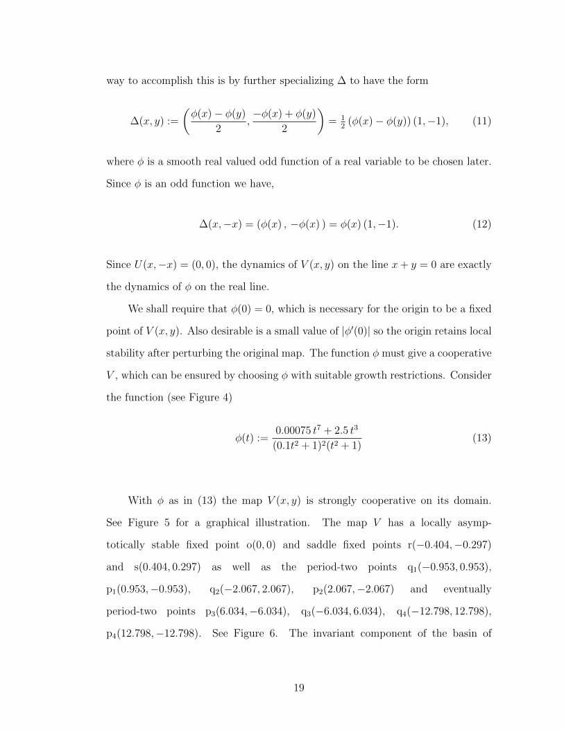
the function (see Figure 4)

φ(t) :=0.00075 t7 + 2.5 t3

(0.1t2 + 1)2(t2 + 1)(13)

With φ as in (13) the map V (x, y) is strongly cooperative on its domain.

See Figure 5 for a graphical illustration. The map V has a locally asymp-

totically stable fixed point o(0, 0) and saddle fixed points r(−0.404,−0.297)

and s(0.404, 0.297) as well as the period-two points q1(−0.953, 0.953),

p1(0.953,−0.953), q2(−2.067, 2.067), p2(2.067,−2.067) and eventually

period-two points p3(6.034,−6.034), q3(−6.034, 6.034), q4(−12.798, 12.798),

p4(12.798,−12.798). See Figure 6. The invariant component of the basin of

19

y = ϕ( t )

y = t

0 a b c dt

a

y

Figure 4. Graphs of φ from (13) and the identity function on the nonnegative semi axis.φ has locally asymptotically stable fixed points 0, b = 2.06, and a repelling fixed pointa = 0.95. The real numbers c = 6.03 and d = 12.80 are pre-images of a. The basin ofattraction of 0 on the semi-axis consists of the intervals 0 ≤ t < a and c < t < d. Alldecimal numbers have been rounded to two decimals.

z = V11(x, y) z = V12(x, y) z = V21(x, y) z = V22(x, y)

Figure 5. The partial derivatives of V (x, y). Also shown in the plane z = 0.

attraction of the origin is bounded by the global stable manifolds of two saddle

fixed points which have endpoints at period-two points.

Example 2 Consider maps of the form

T (x, y) :=

(x3

αx+ (1− α) y,

y3

(1− δ)x+ δ y

), (x, y) ∈ R2

+ \ {0, 0}, α, δ ∈ (0, 1)

(14)

The map T is competitive on its domain and strongly competitive on its interior,

the open positive quadrant, as can be concluded from the jacobian matrix

(x2 ( 2xα+3 y (1−α) )

((αx+(1−α) y)2 − x3 (1−α)((αx+(1−α) y)2

− y3 (1−δ)((δ)x+δ y)2

y2 (2 y δ−3x(δ−1))((1−δ)x+δ y)2

)(15)

The origin o is a singular point, and there are three fixed points, namely

a(α, 0), d(0, δ) and b(1, 1). A straightforward calculation gives that a and d are

20

s

p1 p2

p3

p4

r

q1

q2

q3

q4q1

p1

o

r

s

(a) (b)

Figure 6. (a) Three components of the basin of attraction of the fixed point zero ofthe map V (x, y) in Example 1. Here r, s are saddle fixed points, p1 and q1 are a saddleperiod-two pair, p2 and q2 are repelling fixed points, and p3, p4, q3, q4 are eventualperiod-two points. The boundary of the invariant part of the basin of attraction consistof stable manifolds of saddle fixed points with a period-two endpoints. In addition, thereare two eventually period-two points which are end points of another piece of the basinof attraction which is mapped into the invariant part. (b) The invariant component ofthe basin of the origin o.

saddle points, each with an open semiaxis as unstable manifold. Also b is a repeller,

with characteristic values 2, 4 − α − δ, and corresponding eigenvectors (1, 1) and

(α− 1, 1− δ). The ray {(x, x) : x > 0}, is invariant, more specifically we have

T (x, x) = (x2, x2) for all x > 0, α, δ ∈ (0, 1). (16)

The following is a complete characterization of the global dynamics of map

(14) for all allowed values of the parameters. See Figure 7.

Proposition 1 Let T be as in (14). For all values of α and δ in (0, 1), the set

B := {(x, y) : T n(x, y)→ (0, 0)} is bounded by north-east ordered Lipschitz curves

C+ and C−, which have endpoints a, b and d, b respectively. Also, C+ and C− are

tangential to the line y = x at the point b. If (x, y) 6= b is in C+ (resp. C−) then

21

T n(x, y) → a (resp. T n(x, y) → d), while if (x, y) is in the complement of the

closure of B, then ‖T n(x, y)‖ → ∞.

d

ao

b

C+

C−

B

Figure 7. Global dynamics for map (14) as given in Proposition 1. Here α = 0.4 andδ = 0.7.

Proof. We begin by verifying that the origin has a relative neighborhood that is

a subset of B. This can be seen as follows. The relations T (x, 0) �se (x, 0) for

0 < x < α, and (0, y) �se (0, y) for 0 < y < δ imply that for (u, v) with 0 < u < x

and 0 < v < y, T n(0, y) �se T n(u, v) �se T n(x, 0). Since T n(x, 0) → (0, 0) and

T n(0, y) → (0, 0), we have T n(u, v) → (0, 0). Thus the set O′ = {(x, y) : 0 < x <

α , 0 < y < δ} satisfies O′ ⊂ B. Therefore the hypotheses of Theorems 4, 5 and 6

are satisfied.

We now show that B has only one component. By Theorem 4, all components

of B are non-comparable in the south-east ordering, therefore they are comparable

in the north-east ordering. By (16) the open line segment L := {(x, x) : 0 <

x < 1} consists of points (x, x) such that T n(x, x) → (0, 0). Also by (16) the ray

S := {(x, x) : 1 < x <∞} consists of points (x, x) such that ‖T n(x, x)‖ → ∞. For

any point (z, w) with z > 1 or w > 1 one may choose x so that (x, x) �se (z, w) or

22

(z, w) �se (x, x). It follows T n(x, x) �se T n(z, w) or T n(z, w) �se T n(x, x). Since

T n(x, x) = (x2n, x2

n), we have ‖T n(z, w)‖ → ∞. In particular, it follows that B

has only one component.

Note {a, d, b } ⊂ ∂B. Let C− and C+ be as in Theorem 4. Since no points

outside of the unit square belong to B, it follows that b is an endpoint of both

C+ and C−. Also a is an endpoint of C− and d is an endpoint of C+, due to the

fact that the axes are unstable manifolds of a and d. The rest of the proposition

follows from Theorems 4, 5 and 6, and their corollaries. 2

2.4 Proofs

Proof of Theorem 4. It is sufficient to consider the case where T is strongly

monotonic. To see this, let T , B, k and O be as in Theorem 4, and let Bk :=

{x ∈ int(R) : Tmk(x) → x as m → ∞}. If x ∈ Bk, then Tmk(x) ∈ O for m

large enough, which implies x ∈ B. Thus Bk ⊂ B, and since B ⊂ Bk it follows

B = Bk. Without loss of generality we assume for the rest of this section that T is

a strongly monotonic map (k = 1).

We prove several claims first. The first two claims are about certain properties

of B and its boundary set.

Claim 1 The set B is open and order convex, and it has either a finite or countably

infinite number of connected components.

Proof. If x ∈ B, then for sufficiently large m ∈ N we have Tm(x) ∈ O. Then

x is an element of (Tm)−1(O), which is an open subset of B. Thus B is open.

If {x, z} ⊂ B, then by monotonicity of T , for every y ∈ int(R) and all m ∈ N,

x � y � z implies Tm(x) � Tm(y) � Tm(z). Hence Tm(y)→ x and we conclude B

is order-convex. If the number of connected components of B is not finite, choose

a point in each of the components with rational entries. The collection of such

points is countable, hence so is the collection of components of B. 2

23

Claim 2 The set ∂B does not contain a linearly ordered line segment contained

in int(R).

Proof. Arguing by contradiction, suppose ∂B contains a �ne linearly ordered line

segment L(x, z) ⊂ int(R). Choose y a point In L(x, z) with y 6= x, z. Then T (x) <

<ne T (y) <<ne T (z) by strong monotonicity of T . But then V <<ne T (y) <<ne W

for some open neighborhoods V of T (x) and W of T (z). Now both V and W

contain points in B, say v and w. In particular, v <<ne T (y) <<ne w. Since B is

order-convex, it follows that T (y) ∈ B, which contradicts invariance of ∂B. 2

We now proceed to define functions φ± of a real variable that are key to

establishing further properties of the boundary of B. Denote with π1 the projection

operator on R2 given by π1(x, y) = x. Let I := π1(B), that is, I is the set consisting

of all t in R for which there exists y in R such that (t, y) ∈ B. The set I is open

in R, and it has a finite or countable number of connected components (intervals).

For each connected component of I choose a rational number q in the component,

and label the component as Iq. Let Q be the set consisting of all such indices

q. Then for each q ∈ Q, the sets Iq are open in R, pairwise disjoint, and satisfy

I =⋃q∈Q

Iq. Define for each t ∈ I,

φ−(t) := inf {y : (t, y) ∈ B} and φ+(t) := sup {y : (t, y) ∈ B} . (17)

Note that the definition of φ± implies graph(φ±) ⊂ ∂B and

B = {(t, y) ∈ R : t ∈ I and φ−(t) < y < φ+(t) } . (18)

Properties of φ± are investigated in Claims 3–8 below.

Claim 3 The functions φ± are non-increasing on I.

24

Proof. Suppose this is not the case, so there exist t1, t2 in I, t1 < t2, such that

φ+(t1) < φ+(t2). Choose y1 and y2 so that φ−(t`) < y` < φ+(t`) for ` = 1, 2, and

y2 > φ+(t1). Then (t1, φ+(t1)) belongs to the order interval [(t1, y1), (t2, y2)]. Since

(t`, y`) ∈ B for ` = 1, 2, it follows that (t1, φ+(t1)) ∈ B, which is a contradiction.

Thus φ+ is non-increasing on I. The proof of the corresponding statement for φ−

is similar. 2

For each q ∈ Q the restriction of the function φ− (resp. φ+) to Iq is nonincreasing,

hence it has a natural extension to the closure of Iq in the extended real line given

by choosing the value at each endpoint of Iq as the one-sided limit of φ− (resp.

φ+). We denote such extensions with φq− and φq+. It is a consequence of Claim 3

that for q ∈ Q, the functions φq− and φq+ are non-increasing, and their graphs are

contained in ∂B.

Claim 4 For every q ∈ Q, (i) φq−(t) < φq+(t) for t ∈ Iq, and (ii) φq−(t) = φq+(t)

for t ∈ ∂Iq \ ∂π1(R).

Proof. Statement (i) of Claim 4 follows from the definition of φ±. To prove (ii) of

Claim 4, suppose that for some q ∈ Q and some endpoint t of Iq with t 6∈ ∂π1(R),

the inequality φq−(t) < φq+(t) holds. In this case the line segment joining (t, φ−(t)))

to (t, φ+(t)) is a �ne-linearly ordered subset of ∂B ∩ int(R), which contradicts

Claim 2. Therefore φq−(t) = φq+(t). 2

Claim 5 Each of the sets⋃q∈Q

(graph(φq−) ∩ int(R)) and⋃q∈Q

(graph(φq+) ∩ int(R))

is invariant under T .

Proof. Let t ∈ clos(I). If (t′, y′) := T (t, φ+(t)), then there is a curve in B with

endpoint at (t, φ+(t)), so the same is true about (t′, y′) := T (t, φ+(t)). thus t′ ∈

clos(I). If t′ ∈ ∂I, then φ−(t′) = φ+(t′) by claim 4, so in particular T (t, φ+(t)) ∈

25

graphφ+. Now suppose t ∈ I. For all δ > 0 small enough, (t, φ+(t) − δ) ∈ B and

consequently (t′δ, y′δ) := T (t, φ+(t) − δ) ∈ B. By monotonicity of T , (t′δ, y

′δ) <<ne

(t′, y′). But φ− is non- increasing, so necessarily (t′, y′) ∈ graph(φ+). 2

Claim 6 ∂B ∩ int(R) = int(R) ∩⋃q∈Q

graph(φq−) ∪ graph(φq+) .

Claim 7 For q ∈ Q let φ be either φq− or φq+. If graph(φ) ⊂ int(R), then φ is

decreasing.

Proof. Arguing by contradiction, if φ(t1) ≤ φ(t2) for t1, t2 in clos(I) with t1 <

t2, then T (t1, φ(t1)) <ne T (t1, φ(t2)) by strong monotonicity. The latter relation

together with the invariance of graph(φ) imply that φ is not non-decreasing, a

contradiction. 2

Claim 8 For every q ∈ Q, φq− and φq+ are continuous on clos(Iq).

Proof. Suppose φ+ is not continuous at some t0 in clos(I). By the monotonic

character of φ, the discontinuity is of the “jump” variety. More specifically, assume

that φ+ is defined on an interval t0 < t < t0 + δ for some δ > 0, and y0 > y+,

where y0 := φ+(t0) and y+ := limt→t+0φ+(t). In this case, (t0, y+) ∈ B, which is

not possible. 2

Now we prove statements (i)–(iv) of Theorem 4. Let (α, β) := π1(R) be the

projection of B onto the first coordinate. If B′ is a component of B, then π1(B′) is

an interval such that Iq = π1(B′) for some q ∈ Q. Define the curves C± by cases

as follows (see Figure 8).

(I) If π1(R) and π1(B′) have no common endpoints, C± is the curve given by the

graph of φq±.

26

(II) If π1(R) and π1(B′) have β and only β as common endpoint, C− is the curve

given by the graph of φq− and C+ is the curve given by the graph of φq+

together with the line segment joining (β, φq+(β)) to (β, φq−(β).

(III) If π1(R) and π1(B′) have α and only α as common endpoint, C+ is the curve

given by the graph of φq+ and C− is the curve given by the graph of φq−

together with the line segment joining (α, φq−(α)) to (α, φq+(α).

(IV) If π1(R) and π1(B′) have common endpoints α and β, C+ is the curve given by

the graph of φq+ together with the line segment joining (β, φq+(β)) to (β, φq−(β)

and C− is the curve given by the graph of φq− together with the line segment

joining (α, φq−(α)) to (α, φq+(α).

The different cases are illustrated in Figure 8. Statement (i) of Theorem 4 now

follows from relation (18) and Claims 4, 7 and 8. Statement (ii) of Theorem 4 is a

consequence of the order-convex character of B. Since B∗ is connected and contains

the fixed point x, it follows T (B∗) ⊂ B∗. This fact and Claim 5 imply statement

(iii) of Theorem 4. Now assume the hypothesis of (iv), and choose x ∈ B′. Since

Tm(x) → x, there exists n a positive number in N such that T n(x) ∈ B∗ and

T n−1(x) 6∈ B∗. Now statement (iv) of Theorem 4 follows from the fact that T

maps connected sets to connected sets and from Claim 5. 2

Lemma 1 Let J be a 2 × 2 matrix with positive entries. Let v be an eigenvector

of J that is associated with the eigenvalue of J that has the smallest modulus. Let

C be a closed convex double cone in R2 with vertex at the origin such that v 6∈ C.

Then there exists an integer m such that Jm(C) ⊂ Q1 ∪Q3.

Proof. Let λ1 and λ2 be eigenvalues of J , with associated eigenvectors v1, v2.

Assume |λ1| < λ2. We prove first that Jm(∂C) ⊂ Q1 ∪ Q3. If z ∈ ∂C \ {0}, then

27

C+

C−

C+C−

HHY

AAU

���-

HHY

AAU

AAK-C+

C− C+C− @

@@R

���@@@I

@@@R

�@

@@@I

(I) (II) (III) (IV)

Figure 8. The four cases in the definition of C±.

z = α1 v1 + α2 v2 for some scalars α1, α2 ∈ R with α2 6= 0. Then

Jmz = λm1 α1 v1 + λm2 α2 v2 = λm2

((λ1λ2

)mα1 v1 + α2 v2

)(19)

Note that v2 has both coordinates with the same sign, by Perron-Frobenious The-

orem. Since |λ1λ2| < 1, it follows from (19) that for m large enough, Jmz has

both coordinates with sign equal to the sign of α2. Hence Jmz ∈ Q1 ∪ Q3 and

Jm(∂C) ⊂ Q1 ∪ Q3. Let C be the double cone in R2 that is complementary to

C. Note C ⊂ J(C), similarly C ⊂ Jm(C). The set Jm(C) is a double cone with

boundary in Q1 ∪ Q3, and such that v ∈ Jm(C). Since R2 = (JmC) ∪ (Jm C), it

follows that JmC ⊂ Q1 ∪Q3. 2

Proof of Theorem 5. We present here a proof for the case where the point p is

a fixed point of T . The case where p is a minimal period-m point may be treated

by considering the map Tm, for which p is a fixed point, and it is not given here.

By Theorem 4, B = C− ∪ C+. Without loss of generality we assume p ∈ C+. If

the conclusion is not true, then there exists a double cone C containing ` \ {p} in

its interior and a sequence {xm} on the curve C+ such that xm → p and xm 6∈ C.

Choose an integer m as in Lemma 1, and set Jm :=(a bc d

). Let {(t, φ(t)) : t ∈ I}

28

be a parametrization of C+ near p, such that for some t∗ in the real interval I,

(t∗, φ(t∗)) = p. Set

Ln :=(a (tn − t∗) + b (φ(tn)− φ(t∗)), c (tn − t∗) + d (φ(tn)− φ(t∗))

)(20)

From Lemma 1, Ln ∈ Q1 ∪ Q3. Also, Ln 6= (0, 0), since the null space of J , if

nontrivial, is contained in the cone C. Then,

for each n ≥ 0, Ln has nonzero coordinates with the same sign. (21)

Let K be a compact interval containing t∗ in its interior and define, for t ∈ K and

ε1, ε2 ∈ [−1, 1],

Φ1(t, ε1) :=(

(a+ ε1)(t− t∗) + (b− ε1)(φ(t)− φ(t∗)))

Φ2(t, ε2) :=(

(c+ ε2)(t− t∗) + (d− ε2)(φ(t)− φ(t∗))) (22)

The functions Φ1 and Φ2 are uniformly continuous on K × [−1, 1], and by (21),

Φ1(t, 0) and Φ2(t, 0) are nonzero and have the same sign for all n. By uniform

continuity, there exists δ > 0 such that Φ1(t, ε1) and Φ2(t, ε2) are nonzero and have

the same sign for all t ∈ K and |ε1| < δ, |ε2| < δ. Without loss of generality we

may assume that

tn > t∗ and φ(tn) < φ(t∗), n ∈ N. (23)

Let J and J be the jacobian matrices of of T and Tm at p respectively. Since p is

a fixed point, the chain rule gives J = Jm. Note the entries of J are positive. Set

29

J :=(a bc d

). For each n ∈ N define o

(1)n and o

(2)n by

(o(1)n , o(2)n ) := Tm(tn, φ(tn))− Tm(t∗, φ(t∗))− Ln. (24)

Since T is continuously differentiable,

g(`)n :=o(`)

|tn − t∗|+ |φ(tn)− φ(t∗)|→ 0 as n→∞, ` = 1, 2. (25)

Rearranging terms in (24) and using (20), (23) and (25) we have

Tm(tn, φ(tn))− Tm(t∗, φ(t∗))

=(

(a+ g(1)n )(tn − t∗) + (b− g(1)n )(φ(tn)− φ(t∗)) , c+ g

(2)n + (d− g(2)n )(φ(tn)− φ(t∗))

)(26)

By (21), (23) and (25) and the assumption that a, b, c and d are positive, both

coordinates in the right-hand side of (26) have the same sign for large n, and

therefore either T (tn, φ(tn)) � T (t∗, φ(t∗)) or T (t∗, φ(t∗)) � T (tn, φ(tn)). But this

contradicts (i) of Theorem 4, which requires points on C+ to be non-comparable.

2

Proof of Theorem 6. (i) Let p ∈ C+, and let {(t, φ(t)) : t ∈ I} be a parametriza-

tion of C+ near p, such that for some t∗ ∈ I, (t∗, φ(t∗)) = p. Here I ⊂ R is an

interval. The function φ is decreasing. If φ is not Lipschitz at t∗, then there exists

a sequence {tn} in I such that tn → t∗ and

∣∣∣∣φ(tn)− φ(t∗)

tn − t∗

∣∣∣∣→∞ as n→∞. (27)

Without loss of generality we may assume that tn > t∗ and φ(tn) < φ(t∗) for all n,

that is,

tn ↓ t∗ andφ(tn)− φ(t∗)

tn − t∗→ −∞ as n→∞ (28)

30

Let ( a bc d ) be the jacobian matrix of T at p. For each n ∈ N define o(1)n and o

(2)n by

(o(1)n , o

(2)n ) := T (tn, φ(tn))− T (t∗, φ(t∗))

− (a(tn − t∗) + b(φ(tn)− φ(t∗)), c(tn − t∗) + d(φ(tn)− φ(t∗)))

(29)

Since T is countinuously differentiable,

g(`)n :=o(`)

|tn − t∗|+ |φ(tn)− φ(t∗)|→ 0 as n→∞, ` = 1, 2. (30)

Rearranging terms in (29) and using (28) and (30) we have

T (tn, φ(tn))− T (t∗, φ(t∗))

= (tn − t∗)(a+ g

(1)n + (b− g(1)n )φ(tn)−φ(t∗)

tn−t∗ , c+ g(2)n + (d− g(2)n )φ(tn)−φ(t∗)

tn−t∗

).

(31)

By (28) and (30) and the assumption that a, b, c and d are positive, both co-

ordinates in the right-hand side of (31) are negative for large n, and therefore

T (tn, φ(tn)) � T (t∗, φ(t∗)). But this contradicts (i) of Theorem 4, which requires

points on C+ to be non-comparable. Thus φ is Lipschitz.

(ii) We present the proof for the case when p is a fixed point of T . Note p is

necessarily unstable since p ∈ ∂B. Since it is hyperbolic, it is either a saddle point

or a source. If p is a saddle point, then it has a local stable manifold M s, which is

tangential to v with v not comparable to the origin by the Krein-Rutman theorem.

There exist points x in B∗ that are arbitrarily close to p and which belong to to the

union of quadrants Q2(p) and Q4(p). Furthermore, such points x may be chosen

to be comparable to points on M s, which would prevent the iterates of such points

from converging to p, thus contradicting the definition of stable manifold. 2

31

List of References

[1] A. Brett and M. R. S. Kulenovic, Basins of Attraction of Equilibrium Pointsof Monotone Difference Equations. Sarajevo J. Math., 5(18): 211–233, 2009.

[2] S. Elaydi, An introduction to difference equations. Third edition. Undergrad-uate Texts in Mathematics. Springer, New York, 2005.

[3] M. Garic-Demirovic, M. R. S. Kulenovic and M. Nurkanovic, Basins of At-traction of Certain Homogeneous Second Order Quadratic Fractional Differ-ence Equation, Journal of Concrete and Applicable Mathematics, Vol. 13 (1-2)(2015), 35-50.

[4] J. Guckenheimer and P. Holmes, Nonlinear oscillations, dynamical systems,and bifurcations of vector fields. Revised and corrected reprint of the 1983original. Applied Mathematical Sciences, 42. Springer-Verlag, New York, 1990.

[5] P. Hess, Periodic-parabolic boundary value problems and positivity, PitmanResearch Notes in Mathematics Series, 247. Longman Scientific and Technical,Harlow; copublished in the United States with John Wiley and Sons, Inc., NewYork, 1991.

[6] M. Hirsch and H. Smith, Monotone Dynamical Systems, Handbook of Differ-ential Equations, Ordinary Differential Equations (second volume), 239-357,Elsevier B. V., Amsterdam, 2005.

[7] M. Hirsch and H. L. Smith, Monotone Maps: A Review, J. Difference Equ.Appl. 11(2005), 379-398.

[8] M. R. S. Kulenovic and O. Merino, Global Bifurcations for Competitive Sys-tems in the Plane, Discrete Contin. Dyn. Syst. Ser. B 12(2009), 133–149.

[9] M. R. S. Kulenovic and O. Merino, Invariant manifolds for planar competitiveand cooperative maps, Journal of Difference Equations and Applications, Vol.24 (6) (2018), 898-915.

[10] M.R.S. Kulenovic, O. Merino and M. Nurkanovic, Global dynamics of cer-tain competitive system in the plane, Journal of Difference Equations andApplications, Vol. 18 (12) (2012), 1951-1966.

[11] M.R.S. Kulenovic, S. Moranjkic and Z. Nurkanovic Global Dynamics and Bi-furcation of a Perturbed Sigmoid Beverton-Holt Difference Equation, Mathe-matical Methods in Applied Sciences, 39(2016), 2696–2715.

[12] S. W. McDonald, C. Grebogi, E. Ott and J. A. Yorke, Fractal basin bound-aries. Phys. D 17 (1985), no. 2, 125–153.

[13] J. W. Milnor (2006) Attractor. Scholarpedia, 1(11):1815

32

[14] H. E. Nusse and J. A. Yorke, Basins of attraction. Science 271 (1996), no.5254, 1376–1380.

[15] H. E. Nusse and J. A. Yorke, The structure of basins of attraction and theirtrapping regions. Ergodic Theory Dynam. Systems 17 (1997), no. 2, 463–481.

[16] H. E. Nusse and J. A. Yorke, Characterizing the basins with the most entan-gled boundaries. Ergodic Theory Dynam. Systems 23 (2003), no. 3, 895–906.

[17] H. E. Nusse and J. A. Yorke, Bifurcations of basins of attraction from theview point of prime ends. Topology Appl. 154 (2007), no. 13, 2567–2579.

[18] H.L. Smith, Planar competitive and cooperative difference equations, Journalof Difference Equations and Applications, Vol. 3, No.5-6,335-357,1998.

33

MANUSCRIPT 3

Global Dynamics Results for Discrete Planar Cooperative Maps

M. R. S. Kulenovic1, J. Marcotte and O. Merino

Department of Mathematics,

University of Rhode Island,

Kingston, Rhode Island 02881-0816, USA

Publication status:

Submitted to Journal of Difference Equations and Appl.

Keywords: attractivity, cooperative, map, difference equation, invariant sets,

basin of attraction, periodic points

AMS 2010 Mathematics Subject Classification: 39A10, 39A20, 39A30, 92A15,

92A17

34

Abstract

Sufficient conditions are given for planar cooperative maps to have the qualitative

global dynamics determined solely on local stability information obtained from

fixed and minimal period-two points. The results are given for a class of strongly

cooperative planar maps of class C1 on an order interval. The maps are assumed

to have a finite number of strongly ordered fixed points, and also the minimal

period-two points are ordered in a sense. An application is included.

3.1 Introduction

In this paper we consider a cooperative system of the form

xn+1 = f(xn, yn), yn+1 = g(xn, yn), n = 0, 1, ..., (32)

where the transition functions f, g are non-decreasing in all its arguments and its

corresponding map F = (f, g). Sufficient conditions are given for such planar

cooperative map to have the qualitative global dynamics determined by local sta-

bility information obtained from fixed and minimal period-two points. The results

are given for a class of strongly cooperative planar maps of class C1 defined on an

order interval. The maps are assumed to have a finite number of strongly ordered

fixed points and minimal period-two points. Our results holds in hyperbolic case as

well as in some non-hyperbolic cases as well. Our results are motivated by global

dynamic results for the systems

xn+1 = a xn +b ynδ + yn

yn+1 =c xnδ + xn

+ d yn, n = 0, 1, . . .(33)

35

and

xn+1 = a xn +b y2nδ + y2n

yn+1 =c x2nδ + x2n

+ d yn, n = 0, 1, . . . .(34)

see [3, 4, 5, 17]. System (33) was considered in [3] and it was proved that all

bounded solutions exhibited global attractivity to either the zero equilibrium or

to the unique positive equilibrium. More precisely, it was shown in [3] the global

dynamics of system (33) where a, b, c, d, δ > 0, x0, y0 ≥ 0 is simple and can be de-

scribed in terms of bifurcation theory as the transcritical bifurcation which causes

an exchange of stability when (1− a)(1− d)δ2 − bc passes through the value 0.

The system (34), studied in [4] exhibited the appearance of period-two solu-

tions, which played an important role in the global dynamics of this system. Cases

where provided for such system which had 1, 2 or 3 period-two solutions and in

the last case one of these period-two solutions had substantial basin of attraction

[4]. Papers [3, 4] extensively used the algebraic techniques to find the regions of

existence and stability of equilibrium solutions and period-two solutions. The re-

sults in this paper will be proven through the geometric analysis of the equilibrium

curves and by using some major results about the global stable and unstable man-

ifolds of cooperative systems in the plane [21]-[24]. The results of this paper are

applicable to systems (33) and (34). Our results have immediate extension to the

competitive systems of difference equations in the plane.

The paper is organized as follows. In Section 3.2 we list some basic results

that are relevant to this paper, see [21]-[24]. See also [1, 2, 6, 9, 10, 11, 12, 15,

16, 19, 20, 25, 26, 27, 28] for some related competitive systems. In Section 3.3

we present the three main theorems. In section 3.4 we apply the theorems from

Section 3.3 to a parametrized cooperative system whose transition functions are of

the Holling’s type [17]. Finally the proofs of the results in Section 3.3 are presented

36

in Section 3.5.

3.2 Preliminaries

Let � be a partial order on Rn with nonnegative cone P . For x, y ∈ Rn the

order interval Jx, yK is the set of all z such that x � z � y. We say x ≺ y if x � y

and x 6= y, and x � y if y − x ∈ int(P ). A map T on a subset of Rn is order

preserving if T (x) � T (y) whenever x ≺ y, strictly order preserving if T (x) ≺ T (y)

whenever x ≺ y, and strongly order preserving if T (x)� T (y) whenever x ≺ y.

Let T : R→ R be a map with a fixed point x and let R′ be an invariant subset

of R that contains x. We say that x is stable (asymptotically stable) relative to

R′ if x is a stable (asymptotically stable) fixed point of the restriction of T to

R′. The basin of attraction of a fixed point x, denoted as B(x) is defined as

B(x) = {y : T n(y) → x}. Subsolution (resp. supersolution) for the map T is a

point which satisfies x � T (x) (resp. T (x) � x). A fixed point u ∈ V is said to be

order stable from below if there exists a strictly increasing sequence of subsolutions

vn in V convergent to u. A fixed point u ∈ V is said to be strongly order stable

from below if there exists a strictly increasing sequence of strict subsolutions vn

in V convergent to u. The notions of order stable from above and strongly order

stable from above are defined similarly. A (strongly) order stable fixed point has

the respective stability property from above and below [7].

Throughout this paper we shall use the North-East ordering (NE) for which

the positive cone is the first quadrant, i.e. this partial ordering is defined by

(x1, y1) �ne (x2, y2) if x1 ≤ x2 and y1 ≤ y2 and the South-East (SE) ordering

defined as (x1, y1) �se (x2, y2) if x1 ≤ x2 and y1 ≥ y2.

A map T on a nonempty set R ⊂ R2 which is monotone with respect to the

North-East (NE) ordering is called cooperative and a map monotone with respect

to the South-East (SE) ordering is called competitive. A map T on a nonempty

37

set R ⊂ R2 which second iterate T 2 is monotone with respect to the North-East

(resp. South-East) ordering is called anti-cooperative (resp. anti-competitive).

If T is differentiable map on a nonempty set R, a sufficient condition for T to

be strongly monotone with respect to the NE ordering is that the Jacobian matrix

at all points x has the sign configuration

sign (JT (x)) =

[+ +

+ +

], (35)

provided that R is open and convex.

The next result in [24] is stated for order-preserving maps on Rn. See [14] for

a more general version valid in ordered Banach spaces.

Theorem 7 For a nonempty set R ⊂ Rn and � a partial order on Rn, let T : R→

R be an order preserving map, and let a, b ∈ R be such that a ≺ b and Ja, bK ⊂ R.

If a � T (a) and T (b) � b, then Ja, bK is an invariant set and

i.) There exists a fixed point of T in Ja, bK.

ii.) If T is strongly order preserving, then there exists a fixed point in Ja, bK which

is stable relative to Ja, bK.

iii.) If there is only one fixed point in Ja, bK, then it is a global attractor in Ja, bK

and therefore asymptotically stable relative to Ja, bK.

The following result is a direct consequence of the Trichotomy Theorem, see

[14, 24], and is helpful for determining the basins of attraction of the equilibrium

points.

Corollary 4 If the nonnegative cone of a partial ordering � is a generalized quad-

rant in Rn, and if T has no fixed points in Ju1, u2K other than u1 and u2, then the

38

interior of Ju1, u2K is either a subset of the basin of attraction of u1 or a subset of

the basin of attraction of u2.

Next result is a simple and useful geometric test for checking when the fixed

point of the cooperative map is non-hyperbolic.

Lemma 2 Let (x, y) be an interior fixed point of a cooperative map R(x, y) =

(f(x, y), g(x, y)), and let r be the spectral radius of the Jacobian matrix JR(x, y).

Suppose the tangent lines to f(x, y) = x and g(x, y) = y at (x, y) are not parallel

to one of the axes. Denote with m1 and m2 respectively the slopes of the tangent

lines. The following statements are true:

(i) If 0 < m2 < m1, then r < 1.

(ii) If 0 < m1 = m2, then r = 1.

(iii) If 0 < m1 < m2, then r > 1.

Proof. Without loss of generality assume (x, y) = (0, 0). Let J =(α βγ δ

)be the

jacobian of R at the origin. Note the tangent lines to f(x, y) = x and g(x, y) = y

at (0, 0) are given by αx + β y = x and γ x + δ y = y. Thus the entries of J are

nonzero, and m1 and m2 are respectively the slopes of the lines αx+ β y = x and

γ x + δ y = y. Since m1 = (1 − α)/β and m2 = γ/(1 − δ), from m1 > 0 and

m2 > 0, we obtain 0 < α < 1 and 0 < δ < 1. The characteristic polynomial of J ,

p(t) := t2 − (a + d) t + a d − b c, has real and distinct roots s and r, with |s| < r.

Then,

m1 −m2 =1− αβ− γ

1− δ=

1− α− δ + α δ − β γβ(1− δ)

=p(1)

β(1− δ)(36)

Note the minimum of y = p(t) is attained at t = α+δ2

< 1. If m1 > m2, then

p(1) > 0, which implies r < 1. If m1 = m2, then p(1) = 0, hence r = 1. Similarly,

if m1 < m2, then p(1) < 0, so r > 1 in this case. 2

39

3.3 Main Results

In this section we present three theorems. Theorem 8 gives a qualitative

characterization of global dynamics of a class of bounded planar cooperative maps.

The maps are assumed to have hyperbolic fixed points that are strongly ordered

and to have no minimal period-two points. A result for maps with a non-hyperbolic

fixed point is considered in Theorem 9. If minimal period-two points are present,

Theorem 10 gives information that in many situations is sufficient to produce a

description of the global dynamics of the map.

Suppose R = [a, b] is an order interval in R2, and T : R → R is a given

cooperative map. When the number of fixed points of T is one or two, global

dynamics of T can be determined from basic properties of monotone maps and the

The Trichotomy Theorem [15]. Indeed, since T is continuous andR is compact and

connected, T must have a fixed point. If the fixed point is unique, by monotonicity

of T it is a global attractor. Now suppose T has exactly two fixed points x and y

such that x ≺ y. Then a is a supersolution and b is a subsolution, and therefore

∩∞n=0Tn([a, b]) = [x, y]. The Trichotomy Theorem implies that one fixed point

is order stable and the other one is unstable, with the interior of [x, y] being

attracted to either x or y. For bounded strongly cooperative maps with three or

more hyperbolic strongly ordered fixed points and with no minimal period-two

points, the following result gives a qualitative global dynamics description.

Theorem 8 Let R be an order interval (with respect to the north-east ordering)

in R2. Let T : R → R be a map that is strongly cooperative, bounded, and of

class C1 in the interior of R. Assume (H1) The set F of fixed points of T satisfies

3 ≤ |F| < ∞, (H2) F is strongly ordered, and (H3) F ∩ int(R) consists only of

hyperbolic fixed points.

If T has no minimal period-two points, then there exists an integer k with

40

1 ≤ k ≤ |F| − 2, and there exist k invariant strongly south-east ordered pairwise

disjoint curves C1, . . . , Ck in R such that C` has endpoints in ∂R, C` contains a

fixed point of T and only one. Every orbit in C` converges to the fixed point in C`,

which is a saddle fixed point. Each connected component of R \ ∪{C1, . . . , Ck} is

the basin of attraction of an order stable fixed point.

Corollary 5 If T has no interior repelling fixed points, then every orbit converges

to a fixed point.

The following result is useful in the study of planar cooperative maps with non-

hyperbolic fixed points.

Theorem 9 For a, b ∈ R2 with a ≺ b, let T : [a, b]→ [a, b] be a strongly coopera-

tive map that is of class C1 in the interior of [a, b] and such that

(H1) a and b are fixed points of T , and [a, b] contains a unique interior fixed point

c.

(H2) a and c are order stable from above or b and c are order stable from below.

(H3) There are no minimal period-two points in [a, b].

Then there exists a strongly south-east ordered invariant Lipschitz curve C through

c and with endpoints on the boundary of [a, b], such that each of the two connected

components of [a, b] \ C is a subset of the basin of attraction of a fixed point. Also,

for x ∈ C, T n(x)→ c.

Remark 6 By hypothesis (H1) of Theorem 9, in (H3) it is enough to require

x ∈ Q2(c) ∩ Q4(c). Also, hypothesis (H2) implies that the spectral radius of the

jacobian matrix of T at c equals 1. In particular, c is non-hyperbolic.

41

If a bounded strongly cooperative map T with T : R → R has a minimal

period-two point p, then there exist fixed points a and b such that p is in the

interior of [a, b]. Indeed, just choose x and y in R such that x � z � y for all

y ∈ T (R). Then x � T (x) and T (y) � y, that is, x is a super solution and y

is a sub solution. Both have bounded iterates that satisfy T n(x) ≺ p ≺ T n(y),

for n = 1, 2, . . .. Such iterates must converge to fixed points a and b such that

a ≺ p ≺ b. The next result implies that, under hypotheses that include (among

others) the non-existence of minimal period-four points and the existence of a

unique interior fixed point, the global dynamics picture of T on [a, b] is quite

simple.

Theorem 10 For a, b ∈ R2 with a ≺ b, let T : [a, b] → [a, b] be a strongly

cooperative map that is of class C1 in the interior of [a, b] and such that

(H1) a and b are order stable fixed points of T , and [a, b] contains a unique interior

fixed point c,

(H2) There are no minimal period-four points in [a, b].

(H3) If x ∈ [a, b] satisfies T (x) = c, then x = c.

(H4) The smaller characteristic value of T at each fixed point or minimal period-

two point in [a, b] is not −1.

Then the following statements are true.

(i) If {p1, T (p1)} is a unique minimal period two orbit in [a, b], then c is a

repeller and p1 is a periodic saddle point. The basins of a and b in [a, b]

have a common boundary in the interior of [a, b] which is a strongly south-

east ordered invariant curve C1 that contains {p1, T (p1)} and c, and that has

endpoints in the boundary of [a, b]. If x ∈ C1 satisfies x 6= c, then T n(x) is

attracted to {p1, T (p1)}.

42

(ii) If {p1, T (p1)} and {p2, T (p2)} are the only minimal period two orbits in [a, b]

and if p1 ≺ p2, then the boundary of the basin of a in the interior of [a, b]

is a strongly south east ordered invariant curve C1 that contains {p1, T (p1)}

and c, and the boundary of the basin of b in the interior of [a, b] is a strongly

south east ordered invariant curve C2 that contains {p2, T (p2)} and c, both

C1 and C2 have endpoints on the boundary of [a, b], and C1 ∩ C2 = {c}. The

point c is a repelling fixed point, one of p1, p2 minimal period-two periodic

point is a saddle, and the other is a non-hyperbolic semistable periodic point.

If x ∈ C1 satisfies x 6= c, then T n(x) is attracted to {p1, T (p1)}. If x ∈ C2

satisfies x 6= c, then T n(x) is attracted to {p2, T (p2)}. The region bounded

R1 bounded by C1 and C2 is invariant. If x ∈ R1, then T n(x) is attracted to

the orbit of the non-hyperbolic periodic point.

(iii) Suppose T has exactly k ≥ 3 minimal period-two orbits

{p1, T (p1)}, . . . , {pk, T (pk)} where p1, . . . , pk are hyperbolic and

p1 ≺ p2 ≺ . . . ≺ pk. Then c is a repelling fixed point, k is odd, and

for 1 ≤ ` ≤ k, p` is a periodic saddle if ` is odd, while p` is LAS if ` is even.

There exist strongly south east ordered invariant curves C1, . . . , C 12(k+1) with

endpoints on the boundary of [a, b] such that for i, j ∈ {1, . . . 12(k + 1)} with

i 6= j, Ci ∩ Cj = {c}, {p2i−1, T (p2i−1)} ⊂ Ci, and {p2i, T (p2i)} is a subset of

the open region Ri bounded by C2i−1 and C2i+1. For every x ∈ Ci that satisfies

x 6= c, T n(x) is attracted to {p2i−1, T (p2i−1)}. For every x in Ri, Tn(x) is

attracted to {p2i, T (p2i)}. The region Ri is invariant. The boundary of the

basin of a (respectively, b) in the interior of [a, b] is C1 (resp. Ck).

Remark 7 Suppose in Theorem 10 the map T has a bounded and smooth strongly

cooperative extension T on a domain R which contains [a, b] so that a and b

are locally asymptotically stable, and such that fixed points are strongly ordered

43

and all minimal period-two points are contained in [a, b]. Assume also T has no

minimal period-four points in R, and that the equation T (x) = c has x = c as its

only solution in R. By Theorem 4 in [18] there exist south-east strongly ordered

curves C+(a) through a and C−(b) through b that are part of the boundary of

the basin of a and b respectively, and so that c ∈ C+(a) ∩ C−(b). Thus necessarily

C ⊂ C+(a)∩C−(b). Now endpoints of both C+(a) and C−(b) belong to the boundary

of R, since otherwise any such endpoint is a fixed point or minimal period-two

point, by Corollary 2 in [18]. This is not possible because of the assumptions

on T . Boundedness of T can now be used to prove that points on both C+(a)

and C−(b) have iterates that converge to a minimal period-two point. Finally, we

prove C+(a) = C−(b). If C+(a) and C−(b) are not the same curve, then points x

and y can be chosen in C+(a) and C−(b) respectively so that x ≺ y. Then for all

n ≥ 1, T n(x) ≺ T n(y). But for n large enough, T n(x) and T n(y) both belong to

C, which is strongly ordered in the southeast order. This contradiction completes

the argument.

3.4 Global dynamics of a cooperative system

The purpose of this section is to illustrate the application of the results in

this paper. Consider the following parametrized system of difference equations of

Holling type:

xn+1 =a xn

δ1 + xn+

b y2nδ2 + y2n

yn+1 =c x2n

δ2 + x2n+

d ynδ1 + yn

, n = 0, 1, 2, . . . (37)

44

where a, b, c, d, δ1, δ2 > 0, x0, y0 ≥ 0. Let T : R2+ → R2

+ be the map associated to

(37), that is

T (x, y) =

(a x

δ1 + x+

b y2

δ2 + y2,c x2

δ2 + x2+

d y

δ1 + y

). (38)

The results in Section 3.3 imply that if certain properties of the map in question are

satisfied, then the qualitative global dynamics pictures of T can be deduced from

the study of fixed and periodic points. We now proceed to establish properties of

the parametrized family of maps.

Proposition 2 For a, b, c, d, δ1, δ2 > 0, let e0 := (0, 0) and u := ( aδ1

+ bδ2, cδ2

+ dδ1

).

Then the map T in (38) is bounded and satisfies T (R2+) ⊂ [e0, u], T is strongly

monotonic on its domain and it is smooth on a neighborhood of R2+. The set F of

fixed points of T is strongly ordered, finite, and contains the origin.

Proof. The jacobian matrix of T at (x, y) is

JT (x, y) =

(a δ1

(x+δ1)22 b δ2

(y2+δ2)22 c x δ2

(x2+δ2)2d δ1

(y+δ1)2

)(39)

Since JT (x, y) has positive entries, T is strongly monotonic on R2+. The increasing

character of the coordinate entries of T with respect to each variable gives that T

is bounded with range [0, aδ1

+ bδ2

)× [0, cδ2

+ dδ1

). By direct substitution in (38) we

have the origin e0 is a fixed point for all values of the parameters. Fixed points of

T are common points of the equilibrium curves

(C1) : x =a x

δ1 + x+

b y2

δ2 + y2(40)

(C2) : y =c x2

δ2 + x2+

d y

δ1 + y(41)

45

It is obvious that the origin is a fixed point. Since (40) and (41) may be written as

polynomial (quartic) equations, Bezout’s theorem gives that there are at most 16

fixed points. For (x, y) in the positive quadrant, (40) and (41) may be rewritten

as

y =

√−δ2 x (x+ δ1 − a)

x2 + (δ1 − a− b)x− b δ1, max(a− δ1, 0) < x < A , (42)

x =

√−δ2 y (y + δ1 − d)

y2 + (δ1 − c− d) y − c δ1, max(d− δ1, 0) < x < B , (43)

where A := 12

(a+ b− δ1 +

√(a+ b− δ1)2 + 4 b δ1

)and B :=

12

(c+ d− δ1 +

√(c+ d− δ1)2 + 4 c δ1

). Some basic calculations that we

skip show that (42) defines y as an increasing function of x in [0, A), and (43)

defines x as an increasing function of y in [0, B). Thus the set F of fixed points

of T is linearly ordered in the north-east order, and F ⊂ [0, A)× [0, B). 2

Proposition 2 establishes that the parametrized family of maps (38) satisfies

some of the hypotheses of the results in Section 3.3. The remaining hypotheses

concern fixed and periodic points. In the present case, number and type of fixed

and periodic points naturally depends on the choice of parameters that appear

in the definition of the map. Equations (40) and (41) are to be solved to obtain

fixed points, but these equations do not lend themselves to a simple criterion

for classifying fixed points; the number of parameters is just too high and the

polynomial equations that can be obtained have a high degree.

Numerical searches performed by the authors of this article suggest that four

is the maximum number of fixed points for system (37), and that three is the

maximum number of minimal period-two orbits.

In the rest of this section we illustrate the application of the results of this

paper for different parameter choices given in Table 1. The different cases are

46

presented in Figures 9 – 14. For specific values of the map T , fixed points and

minimal period-two points can be easily found with a computer algebra system

(CAS). Also a CAS can be used to determine that a specific fixed point has only

one pre-image. CAS do not work to investigate existence of minimal period-four

points algebraically due to the complexity of the equations involved. In this case

one can use other means such as the approach mentioned in Figure 15.

Case a b δ1 c d δ2(1) 0.345 2 1.585 1.04 0.435 0.73(2) 0.500 2 1.585 0.65 0.435 0.73(3) 0.375 2. 0.98 0.505 1.098 0.73(4) 0.347447 5.26514 4.54021 0.774986 0.137048 9.06053(5) 0.277479 8.91088 0.115188 3.74014 0.4013 7.43602(6) 0.277479 8.91088 3.39209 0.331034 0.115188 7.43602

Table 1. Parameter values used in Figs. 9 – 14

47

0 1 20

1

2

e0

e1

C1

C2

0 1 20

1

2

e0

e1

C

(a) (b)

Figure 9. Case 1 in Table 1. There exists a unique interior fixed point e1, which isnon-hyperbolic and stable from above. The origin e0 is stable from above. There are nominimal period-two points. (a) shows the equilibrium curves, which have a tangentialcontact point at e1, as implied by Lemma 2. (b) By Theorem 9 applied to the restrictionof the map to the invariant order interval [e0,u], there exists a southeast ordered curveC through e1, such that points below C are attracted to e0 and points on or above C areattracted to e1. Since there are no period-two points outside [e0, u], the curve C has anextension to a southeast ordered curve on R2

+ with endpoints on the boundary whichseparates the basins of attraction of e0 and e1.

3.5 Proofs of Theorems

Proof of Theorem 8. Denote with x`, ` = 1, . . . ,m the fixed points of T ordered

so that x` ≺ x`+1, for 1 ≤ ` ≤ m − 1. Choose ` ∈ {1, . . . ,m − 1}. Then [x`, x`+1]

has only two fixed points, so by the Trichotomy Theorem one of the fixed points

is stable and the other is unstable. Thus either all even indexed fixed points are

stable, or all odd indexed fixed points are stable. By boundedness of T , interior

unstable fixed points belong to an order interval in R determined by two stable

fixed points. Suppose x` and x`+2 are stable, and x`+1 is unstable. By Theorem 4

and Theorem 6 in [18] there exist south-east ordered Lipschitz curves C`+, C`−, such

that ∂B(x`) = C`+ ∪ C`−, and whose only possible common points are endpoints,

and in this case such points are either fixed points or minimal period-two points.

Neither of those two possibilities is allowed by the hypotheses of the Theorem,

hence endpoints do not coincide. Note that x`+1 ∈ C`+. Thus the dynamics of T

48

0 1 20

1

2

e0

e1

e2

C1

C2

e0

e1

e2

C

(a) (b)

Figure 10. Case 2 in Table 1. There exist interior fixed points e1 (unstable) and e2(stable). The origin e0 is stable. There are no minimal period-two points. (a) showsthe equilibrium curves, which have a nontangential contact points at e1 and e2. Eithera calculation or Lemma 2 may be used to determine local stability of e1 and e2. (b)By Theorem 9 applied to the restriction of the map to the invariant order interval[e0, e2], there exists a southeast ordered curve C through e1, such that points below Care attracted to e0 points above C are attracted to e2, and points on C are attracted toe1. Since there are no period-two points outside [e0, e2], the curve C has an extension toa southeast ordered curve on R2

+ with endpoints on the boundary which separates thebasins of attraction of e0 and e2.

on the curve C`+ and C`− is one-dimensional, bounded, with only one fixed point,

namely x`+1 and no minimal period-two points. By Theorem C.3 in [8], the iterates

of each point on C`+ must converge to a fixed point. Such point can only be x`+1.

We conclude that x`+1 is a saddle point. A similar argument can be made with

the point x`+1 and the curve C`+2− . Thus C`+ and C`+2

− coincide with a section of the

local stable manifold W sloc of T at x`+1. We claim that C`+ = C`+2

− . To prove this,

assume the contrary statement. Then there exist points x ∈ C`+ and y ∈ C`+2− such

that x ≺ y. Hence T n(x) ≺ T n(y) for all n ≥ 1. Now for n large enough, both

T n(x) and T n(y) enter W sloc, which is strongly ordered in the south-east order, so in

particular T n(x) and T n(y) are not comparable in the north-east order. It follows

that C`+ = C`+2− . 2

Proof of Theorem 9 Assume both a and c are order stable from above. By The-

orem 4 in [18] the boundary of the basin of attraction of a is a strongly south-east

49

0 0.5 10

0.5

1

e0

e1

e2

e3

C1

C2

0 0.5 10

0.5

1

e0

e1

e2

e3

C

(a) (b)

Figure 11. Case 3 in Table 1. There exist hyperbolic interior fixed points e1 (stable), e2(unstable) and e3 (stable). The origin e0 is unstable. There are no minimal period-twopoints. (a) shows the equilibrium curves, which have a nontangential contact points ate`, ` = 1, 2, 3. Either a calculation or Lemma 2 may be used to determine local stabilityof interior fixed points. (b) By Theorem 9 applied to the restriction of the map to theinvariant order interval [e0, e3], there exists a southeast ordered curve C through ee, suchthat non-zero points below C are attracted to e1, points above C are attracted to e2, andpoints on C are attracted to e2. Since there are no period-two points outside [e0, e3],the curve C has an extension to a southeast ordered curve on R2

+ with endpoints on theboundary which separates the basins of attraction of e1 and e3.

ordered curve C. By the strong monotonicity of T and the Trichotomy Theorem,

c ∈ C, [a, b] \ {b} ⊂ B(a), and [c, b] \ {c} ⊂ B(b). The dynamics of the restriction

of T to C is one-dimensional on a compact interval with only one fixed point. Thus

for every x in C, T n(x) converges to c. Now for every y above C with y 6= b, there

exists x in C such that x ≺ y and consequently T n(x) ≺ T n(y). Since T n(x) → c,

then accumulation points z of {T n(y)} satisfy c � z. Now if z 6= c, then T (z)

belongs to the interior of [c, b]. Thus T n(y) enters [c, b] for some n ∈ N, and

therefore it converges to b. 2

Lemma 3 Let a, b be fixed points of T with a ≺ b such that a and b are order stable

with respect to [a, b], and such that there exists a unique fixed point c of T satisfying

a ≺ b ≺ c. Suppose C := ∂B(a) ∩ [a, b] has one and only one minimal period-

two orbit {p, T (p)}, and C has no minimal period-four points. If both smallest

characteristic values of T 2 at c and at p are not ±1, then c is a repeller and p is

50

e0

e1

e2

e3T (p1)

p1

C

Figure 12. Case 4 in Table 1. T has hyperbolic fixed points e0, e1, e2, e3, of whiche1 and e3 are LAS, e0 and e2 are repellers. Also T has minimal period-two pointsp1, T (p2), which are saddle points. Also, {p1, T (p2)} ⊂ [e1, e3]. By Theorem 10,there exists a south-east ordered curve C that separates the basins of e1 and e3 in[e1, e3] and which contains p1, e2, T (p1). By Remark 7 the curve C has an extensionwith endpoints on the boundary of the nonnegative quadrant. Points on C otherthan e2 are attracted to the period-two orbit {p1, T (p1)}.

e0e1

e2

e3

T (p1)

p1

T (p2)

p2C2

C1Figure 13. Case 5 in Table 1. Theorem 10 guarantees the existence of curves C ′1and C ′2 in [e1, e3] and through the period-two points and the point e2. These curvesseparate [e1, e3] in regions attracted to e1, e3, and {p2, T (p2)}. Theorem 4 andCorollary 2 in [18] implies that C ′1 and C ′2 can be extended to invariant curves C1and C2 that bound the basin of attraction of e1 and e3 in R2

+ respectively. C1 andC2 are south-east ordered and extend to the boundary of R2

+. The restriction ofthe map T 2 to each of the curves C1 and C2 exhibits one-dimensional dynamics ofa bounded map on the real line that has two fixed points and no minimal period-two points. By Theorem C.3 in [8], iterates of points on C1 and C2 must convergeto a fixed point of T 2. The point e2 is a repeller with only itself as pre-image.Consequently for ` = 1, 2, for every point x in C` \ {e2} T n(x) is attracted to{p`, T (p`)}. In particular, iterates of points x ∈ (C1 ∪ C2) \ [e1, e3] must enter[e1, e3] after a finite number of iterations. Since for every z in region between thecurves there exist x ∈ C1 and y ∈ C2 such that x ≺ y ≺ z, Then T n(z) must enter[e1, e3], and it is attracted to the nonhyperbolic minimal period two orbit. Thecurves C1 and C2 separate R2

+ into regions attracted to e1, e3, and {p2, T (p2)}.

51

e0

e1

e2

e3T (p3)

p1 p2

p3T (p1)

T (p2)

C2

C1Figure 14. Case 6 in Table 1. T has hyperbolic fixed points e0, e1, e2, e3, ofwhich e1 and e3 are LAS, e0 and e2 are repellers. Also T has minimal period-twopoints p1, T (p1), p3, T (p3) (saddle points), and p2, T (p2) (LAS). Also, all minimalperiod-two points are in [e1, e3]. By Theorem 10, there exist south-east orderedcurves C1 through e2, p1, T (p1) and C2 through e2, p2, T (p2). Iterates of pointson C` other than e2 are attracted to the orbit {p`, T (p`)}, and points between thecurves are attracted to {p2, T (p2)}. The curves C1 and C2 are part of the boundaryof the basin of e1 and e3 respectively, thus by by Remark 7 they have an extensionto the boundary of the nonnegative quadrant.

a saddle point or a non-hyperbolic point of stable type. Furthermore, if no points

in C \ {c} are mapped by T to c, then under iteration by T every point in C \ {c}

is attracted to {p, T (p)}. An analogous statement holds true for the point b.

Proof. By Theorem 2 in [18], C is a strongly ordered curve in the south-east

ordering, with endpoints in ∂[a, b]. Due to strong monotonicity of T , the {p, T (p)}

is a subset of the interior of [a, b]. We need the following statement.

Claim: Suppose z is a fixed point or minimal period-two point of T in C, and

let τ and ρ be the characteristic values of T 2 at z, where |τ | < ρ. If τ < 1, then

in every neighborhood V of y there exist x, y ∈ C ∩ V such that x <<se T4(x) ≤se

z ≤se T 4(y) <<se y, and if τ > 1, then in every neighborhood V of z there exist

x, y ∈ C ∩ V such that T 4(x) <<se x ≤se z ≤se y <<se T4(y). By Theorem 3 in

[18], C is tangential at z to the eigenspace associated to the characteristic value τ .

The claim follows from this fact.

The set C ′ := C ∩ Q4(c) is an unordered closed curve with c at one endpoint

52

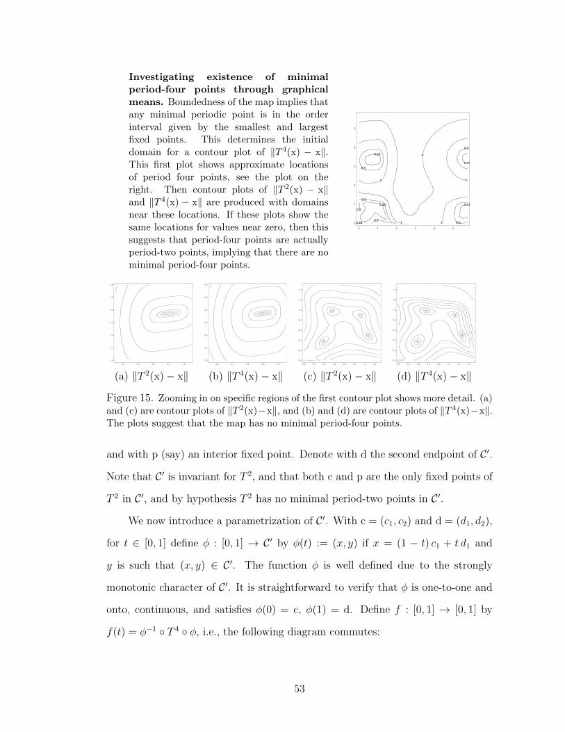
Investigating existence of minimalperiod-four points through graphicalmeans. Boundedness of the map implies thatany minimal periodic point is in the orderinterval given by the smallest and largestfixed points. This determines the initialdomain for a contour plot of ‖T 4(x) − x‖.This first plot shows approximate locationsof period four points, see the plot on theright. Then contour plots of ‖T 2(x) − x‖and ‖T 4(x) − x‖ are produced with domainsnear these locations. If these plots show thesame locations for values near zero, then thissuggests that period-four points are actuallyperiod-two points, implying that there are nominimal period-four points.

0.25

0.25

0.25

0.25

0.25

0.5

0.5

0.5

0.5

0.5

0.5

1.

1. 1.

1.

2.

0 1 2 3 4 5

0

1

2

3

4

5

0.2 0.4 0.6 0.8 1.0

3.0

3.1

3.2

3.3

3.4

3.5

3.6

0.2 0.4 0.6 0.8 1.0

3.0

3.1

3.2

3.3

3.4

3.5

3.6

0.0 0.2 0.4 0.6 0.8 1.0 1.2 1.4

0.0

0.2

0.4

0.6

0.8

1.0

1.2

1.4

0.0 0.2 0.4 0.6 0.8 1.0 1.2 1.4

0.0

0.2

0.4

0.6

0.8

1.0

1.2

1.4

(a) ‖T 2(x)− x‖ (b) ‖T 4(x)− x‖ (c) ‖T 2(x)− x‖ (d) ‖T 4(x)− x‖

Figure 15. Zooming in on specific regions of the first contour plot shows more detail. (a)and (c) are contour plots of ‖T 2(x)−x‖, and (b) and (d) are contour plots of ‖T 4(x)−x‖.The plots suggest that the map has no minimal period-four points.

and with p (say) an interior fixed point. Denote with d the second endpoint of C ′.

Note that C ′ is invariant for T 2, and that both c and p are the only fixed points of

T 2 in C ′, and by hypothesis T 2 has no minimal period-two points in C ′.

We now introduce a parametrization of C ′. With c = (c1, c2) and d = (d1, d2),

for t ∈ [0, 1] define φ : [0, 1] → C ′ by φ(t) := (x, y) if x = (1 − t) c1 + t d1 and

y is such that (x, y) ∈ C ′. The function φ is well defined due to the strongly

monotonic character of C ′. It is straightforward to verify that φ is one-to-one and

onto, continuous, and satisfies φ(0) = c, φ(1) = d. Define f : [0, 1] → [0, 1] by

f(t) = φ−1 ◦ T 4 ◦ φ, i.e., the following diagram commutes:

53

[0, 1]

φ��

f // [0, 1]

φ��

C ′ T 4// C ′

Thus f has exactly two fixed points, namely 0 and a fixed point t∗ ∈ (0, 1)

where φ(t∗) = p. Note by the hypothesis on the point c the relation f(t) = 0 is only

satisfied by t = 0. To see that p is not a repeller, assume it is. By the Claim above,

the function f(t) satisfies f(t) > t for t ∈ (t∗, d1], which is not possible. Thus p is

locally asymptotically stable or non-hyperbolic of stable type. In particular, t∗ is

locally asymptotically stable for f(t). We now prove that c is a repeller. Assume

the contrary, i.e., c is a saddle point. By the Claim and the fact that f(t) has only

two fixed points, it follows that f(t) < t for t ∈ [c1, t∗). But this contradicts the

Claim’s conclusion of p being locally asymptotically stable. Thus c is a repeller.

Finally, by Theorem C.3 in [8] applied to f(t) on [0, 1], under iteration of f

every point in [0, 1] converges to 0 or t∗. But the basin of 0 consists of 0 only.

Thus every point other than 0 converges under iteration to t∗, which implies the

last statement in the Lemma. 2

The following result is a corollary to P. Hartman’s Lemma 5.1 and Corollary 5.1

in [13].

Lemma 4 Let c ∈ R2 be a fixed point of a planar map F which is of class C1 in a

neighborhood of c. Suppose that the characteristic values of F at c are real numbers

τ and ρ such that |τ | < min(1, ρ). Then there exists a C1 curve C∗ through c that

is locally invariant under F which is tangential to the eigenspace V associated with

τ , such that for any x, if x ∈ C∗ then T n(x) → c, and if x 6∈ C∗ and F n(x) → c

tangentially to V, then there exists n0 ∈ N such that F n(x) ∈ C∗ for n ≥ n0.

Proof. There is no loss of generality in assuming c = (0, 0) and that the map F

54

has the form

F (x, y) = (τ x+ f1(x, y), ρ y + f2(x, y)) (44)

where f1, f2 and their first partial derivatives are all zero at (0, 0). By Hartman’s

Lemma 5.1 there exists a function y = φ(x) of class C1 for small |x| satisfying

φ(0) = φ′(0) = 0, and such that the graph of φ is locally invariant under F . By

the same Lemma it may be assumed φ(x) = 0 and f2(x, 0) = 0 for small |x|,

by performing a C1 change of variables if necessary. The curve C∗ is now taken

to consist of points x = (x, 0) with small |x|. Choose a real number θ0 so that

0 < θ0 < min(ρ−τ4, 1−τ

2). If x = (x, 0) ∈ C∗, then F (x, 0) = (τ x + f1(x, 0), 0), and

by the proof of Corollary 5.1 in page 238 of [13], |F (x, 0)| < (τ + θ0)|x| < 1+τ2|x|.

Hence F n(x)→ (0, 0). Now consider x such that (xn, yn) := F n(x) satisfies xn 6= 0

for all n ≥ 0, (xn, yn) → (0, 0) and yn/xn → 0. To complete the proof it must be

shown that yn = 0 for all large enough n. If for some m the point (xm, ym) satisfies

ym = 0 and |xm| is small enough, then ym+k = 0 for k = 0, 1, 2, . . . and there is

nothing else to prove. Now assume yn 6= 0 for all n ≥ 0. The proof of Corollary

5.1 in page 238 of [13] gives the inequality |yn+1| ≥ (ρ − 2θ0) |yn|, which by the

definition of θ0 implies

|yn+1| ≥ 12(ρ+ τ) |yn|. (45)

Since f1(x, y) and its derivatives are zero at the origin, we have

f1(xn, yn)

xn=o(|xn|+ |yn|)

xn= o

(1 + | yn

xn|). (46)

The assumption yn/xn → 0 and (46) imply that there exists n0 ∈ N such that

f1(xn, yn)

xn≤ 1

2(ρ− τ) , n = n0, n0 + 1, . . . (47)

55

From (44) and (47),

|xn+1| = |τ xn + f1(xn, yn)| ≤ (τ + |f1(xn, yn)/xn|) |xn|≤ (τ + 1

2(ρ− τ))|xn| = 1

2(ρ+ τ)|xn|

, n = n0, n0+1, . . .

(48)

Combine (45) and (48) to obtain

∣∣∣∣ yn+1

xn+1

∣∣∣∣ ≥ ∣∣∣∣ ynxn∣∣∣∣ , n = n0, n0 + 1, . . . , (49)

which contradicts the assumptions yn 6= 0 and yn/xn → 0. Thus (xn, yn) ∈ C∗ for

all n large enough. 2

Proof of Theorem 10. Lemma 3 and Theorem 3 in [18] imply most of

statement (i), the only thing left to verify is that ∂B(a) = ∂B(b). By Lemma 4

there is an invariant local curve C∗ through p that is tangential to the eigenvector

associated with the smallest characteristic value of T at p. Since {p, p′} ⊂ ∂B(a)∩

∂B(b), we have C∗ ⊂ ∂B(a) ∩ ∂B(b). Arguing by contradiction, suppose ∂B(a) 6=

∂B(b). Then there exist x ∈ C1, y ∈ C2 such that x <ne y neither point is a

fixed point or a period-two point. Iterates T n(x) and T n(y) eventually enter C∗

by Lemma 4, so either they are non-comparable, or they are the same point. But

either possibility is not allowed by the strongly cooperative character of the map

T . Thus ∂B(a) = ∂B(b).

To prove (ii), consider p1 and p2 as fixed points of the strongly cooperative

map T 2. Set C ′` := C` ∩Q4(C), ` = 1, 2. Assume p1 is a saddle point.

Since p1 � p2, The Trichotomy Theorem [14] and p1 being a saddle imply

that [p1, p2] \ {p1} ⊂ B(p2). By Lemma 3, C ′` \ {C} ⊂ B(p`), ` = 1, 2. If x is

a point in the (interior of) region between C ′1 and C ′2, there exist points y1 ∈ C ′1

and y2 ∈ C ′2 such that y1 � x � y2. Therefore T 2n(y1) � T 2n(x) � T 2n(y2) for

56

n = 1, 2, . . .. Since T 2n(y`)→ p` for ` = 1, 2, for n large enough T 2n(x) ∈ [p1, p2],

and consequently T 2n(x)→ p2 and T n(x)→ p2 as well. This completes the proof

of (ii).

To prove (iii), note that for T 2, the points p1 and p3 are saddle points and

consequently p2 is locally asymptotically stable. Note that [p1, p3] \ {p1, p3} ⊂

B(p2). The argument used in the proof of part (ii) can be used here to conclude

that the region between C ′1 and C ′2 is precisely the basin of p2 as a fixed point of

T 2. This completes the proof of the theorem. 2

List of References

[1] L. J. S. Allen, An Introduction to Mathematical Biology, Prentice Hall, (2006).

[2] L. Assas, G. Livadiotis, S. Elaydi, E. Kwessi and D. Ribble, Competitionmodels with Allee effects, J. Difference Equ. Appl., 20(2014), 1127–1151.

[3] A. Bilgin and M. R. S. Kulenovic, Global Asymptotic Stability for DiscreteSingle Species Population Models, Discrete Dyn. Nat. Soc., Volume 2017,(2017), 15 p.

[4] A. Bilgin, A. Brett, M. R. S. Kulenovic and E. Pilav, Global Dynamics of ACooperative Discrete System in the Plane, Int. J. of Bifurcations and Chaos,28(2018), 17p.

[5] A. Brett and M. R. S. Kulenovic, Two Species Competitive Model with theAllee Effect, Advances in Difference Equations, Volume 2014 (2014):307, 28p.

[6] J. M. Cushing, S. Levarge, N. Chitnis and S. M. Henson, Some discrete com-petition models and the competitive exclusion principle , J. Difference Equ.Appl. 10(2004), 1139-1152.

[7] E.N. Dancer and P. Hess, Stability of fixed pionts for order-preserving discrete-time dynamical systems, J. reine. angew. Math. 49(1991), 125-139.

[8] S. Elaydi, An introduction to difference equations. Third edition. Undergrad-uate Texts in Mathematics. Springer, New York, 2005.

[9] J. E. Franke and A-A. Yakubu, Mutual exclusion versus coexistence for dis-crete competitive systems, J. Math. Biol. 30(1991), 161–168.

57

[10] J. E. Franke and A-A. Yakubu, Global attractors in competitive systems,Nonlin. Anal. TMA 16(1991), 111–129.

[11] J. E. Franke and A-A. Yakubu, Geometry of exclusion principles in discretesystems, J. Math. Anal. Appl. 168(1992), 385–400.

[12] J. Guckenheimer, John and P. Holmes, Nonlinear oscillations, dynamical sys-tems, and bifurcations of vector fields. Revised and corrected reprint of the1983 original. Applied Mathematical Sciences, 42. Springer-Verlag, New York,1990.

[13] P. Hartman, Ordinary Differential Equations, 2nd. Ed., SIAM 2002.

[14] P. Hess, Periodic-parabolic boundary value problems and positivity, PitmanResearch Notes in Mathematics Series, 247. Longman Scientific and Technical,Harlow; copublished in the United States with John Wiley and Sons, Inc., NewYork, 1991.

[15] M. Hirsch and H. Smith, Monotone Dynamical Systems, Handbook of Differ-ential Equations, Ordinary Differential Equations (second volume), 239-357,Elsevier B. V., Amsterdam, 2005.

[16] M. Hirsch and H. L. Smith, Monotone Maps: A Review, J. Difference Equ.Appl. 11(2005), 379-398.

[17] C. S.Holling, “The functional response of predators to prey density and itsrole in mimicry and population regulation,” Memoirs of the EntomologicalSociety of Canada, vol. 97, supplement 45, pp. 5–60, 1965.

[18] M. R. S. Kulenovic, J. Marcotte and O. Merino, Properties of Basins of At-traction for Planar Discrete Cooperative Maps, (to appear).

[19] M.R.S. Kulenovic and O. Merino, Discrete Dynamical Systems and DifferenceEquations with Mathematica, Chapman & Hall/CRC, Boca Raton, London,2002.

[20] M.R.S. Kulenovic and O. Merino, A Global Attractivity Result for Maps withInvariant Boxes, Discrete Contin. Dyn. Sys. B,6(2006), 97–110.

[21] M.R.S. Kulenovic and O. Merino, Competitive-exclusion versus competitive-coexistence for systems in the plane, Discrete Contin. Dyn. Sys. B,6(2006),1141–1156.

[22] M.R.S. Kulenovic and O. Merino, Global bifurcations for competitivesystemin the plane, Discrete Contin. Dyn. Syst. Ser. B 12 (2009), 133–149.

[23] M.R.S. Kulenovic and O. Merino, Invariant manifolds for competitive discretesystems in the plane, Int. J. Bifur. Chaos 20 (2010),2471-2486.

58

[24] M.R.S. Kulenovic and O. Merino, Invariant curves for planar competitive andcooperative maps, J. Difference Equ. Appl., Vol. 24 (6) (2018), 898-915.

[25] Robert M. May, Stability and Complexity in Model Ecosystems, PrincetonUniversity Press Princeton, NJ, 2001. xx+292 pp.

[26] H. L. Smith, Planar competitive and cooperative difference equations. J. Dif-fer. Equations Appl. 3 (1998), 335–357.

[27] A-A. Yakubu, The effect of planting and harvesting on endangered species indiscrete competitive systems, Math. Biosci. 126(1995), 1–20.

[28] A-A. Yakubu, A discrete competitive system with planting, J. Difference Equ.Appl., 4(1998), 213–214.

59

MANUSCRIPT 4

Cones for Coordinate-wise Monotone Functions and Dynamics ofMonotone Maps

M. R. S. Kulenovic1, J. Marcotte and O. Merino

Department of Mathematics,

University of Rhode Island,

Kingston, Rhode Island 02881-0816, USA

Publication status:

In preparation for submission to International Journal of Difference Equations.

Keywords: global attractivity, invariant, manifold, monotone, stability

AMS 2010 Mathematics Subject Classification: 37D10, 39A10, 39A20, 39A30

60

Abstract

In this paper we give a characterization of monotone discrete systems of equations

in terms of an associated matrix and give some properties of certain invariant

surfaces of codimension 1, which often give the boundary of the basin of attraction

of certain fixed points. We present several examples that illustrate our results in

the case of k dimensional systems where k ≥ 3.

4.1 Introduction and Preliminaries

In this paper we consider the maps on Rn which are coordinate-wise monotonic

and we characterize those maps which are monotone to a standard ordering ≤σ of

Rn. In two dimensional case the obtained characterization will coincide with two

classes of maps known as competiive and cooperative for which there is an extensive

theory developped in [9, 10, 11, 17, 18, 19, 20, 21, 27]. A map T = (f(x, y), g(x, y))

is called competitive if f(x, y) is non-decreasing in x and non-increasing in y and

g(x, y) is non-increasing in x and non-decreasing in y and it is called cooperative

if both functions f, g are non-decreasing in x and y. This fact can be illustrated

by using the signature matrices

(1 11 1

),

(1 −1−1 1

)(50)

for cooperative and competitive case respectively. Here 1(resp. −1) means that

the corresponding function is non-decraesing (resp. non-increasing) in its argu-

ment. As it was shown in sequence of papers [17, 18, 19, 20, 21, 27] cooperative

and competitive maps in the plane have a lot of structure which leads to charac-

terization of the global stable and unstable manifolds of all hyperbolic fixed and

periodic points which in turn gives the boundaries of the basins of attraction of

such points. In addition the union of global unstable manifolds gives the carrying

61

simplex that majority of solutions follow to the attracting fixed or periodic points.

We were also able to obtain similar results for some non-hyperbolic fixed and peri-

odic points, see [19, 20]. In this paper we will try to extend some of the results in

[17, 18, 19, 20] to the case of maps in Rn, n ≥ 3. The major difficulty in this process

is description of the boundary of an invariant surface which plays the role of global

stable manifold in two dimensional case. While in two dimensional case the global

stable manifolds are continuous curves their boundaries are always either fixed or

periodic points or points on the boundary in higher dimensional case the global

stable manifolds are surfaces which boundaries could have complicated structure,

that makes the problem of their description harder. In this paper we will first

characterize the maps monotone with respect to a standard ordering in Rn among

all coordinate-wise monotonic maps and then we will obtain the description of a

certain invariant manifold, which plays the role of global stable manifold. We will

illustrate our results with several examples. The next example demonstrate use of

techniques from [17, 18, 19, 20] in proving global dynamics of a two-dimensional

competitive map:

Example 3 Consider the system of difference equations

xn+1 =b1xn

1 + xn + c1yn, yn+1 =

b2yn1 + c2xn + yn

n = 0, 1, . . . (51)

where the parameters b1, b2, c1, and c2 are positive real numbers and the initial

conditions x0 and y0 are arbitrary non-negative numbers.

In a modelling setting, system (51) is well-known Leslie-Gower system [3] and

is one of discrete version of Lotka-Volterra system of differential equations [16].

The state variables xn and yn denote population sizes during the n-th generation,

and the sequence {(xn, yn) : n = 0, 1, 2, ...} depicts how the populations evolve

over time. Competition between the two populations is reflected by the fact that

62

the transition function for each population is a decreasing function of the other

population size.

Global behavior of (51) was considered in [3], and global behavior of related

systems was considered in [1, 2, 6, 7, 18] and [19].

It has been shown in [3, 18] that under hypotheses

b1 > 1, b2 > 1 (52)

and

b1 > 1 + c1(b2 − 1), b2 > 1 + c2(b1 − 1), (53)

equation (51) has four equilibrium points: E0(0, 0), E1(b1−1, 0), E2(0, b2−1), and

E3

(b2 − 1

c1c2 − 1

(c1 −

b1 − 1

b2 − 1

),b1 − 1

c1c2 − 1

(c2 −

b2 − 1

b1 − 1

)).

Theorem 4 in [3] states that E1 and E2 are saddle points, E3 is locally asymptoti-

cally stable, and E0(0, 0) is a repeller. The same theorem states that E3 is globally

asymptotically stable, but the proof of this statement given in [3] is incomplete

and it was completed in [19].

Theorem 11 Consider system (51) subject conditions (52) and (53). Then ev-

ery solution which starts in the interior of the positive quadrant converges to the

positive equilibrium E3.

Proof. We begin the proof by showing that the stable manifolds of E1 and E2 do

not intersect the interior of the positive quadrant; more precisely,

{(x, 0) : x ≥ 0} = W s(E1), {(0, y) : y ≥ 0} = W s(E2). (54)

Clearly, if x0 = 0 then xn = 0 for every n = 1, 2, . . . and if y0 = 0 then yn = 0 for

63

every n = 1, 2, . . . . Thus the global stable manifolds of the equilibrium points E1

and E2 satisfy:

{x : x ≥ 0} ⊂ W s(E1), {y : y ≥ 0} ⊂ W s(E2).

In view of the uniqueness of the global stable manifold which follows from the

Stable Manifold Theorem and the Hartman-Grobman Theorem, see [5], we obtain

(54).

It is clear from (51) that xn+1 ≤ b1 and yn+1 ≤ b2 for n = 0, 1, 2, . . .. Therefore,

without loss of generality we may drop the first term of the sequence if necessary,

and assume (x0, y0) belongs to the rectangle D := (0, b1] × (0, b2]. We shall need

the sets D1 := (0, b∗1)× (0, b∗2) , D2 := D \D1, and L := {(x, y) ∈ D : 1 +x+ c1y =

b1 or 1 + y + c2x = b2}, where b∗1 = b2−1c2

and b∗2 = b1−1c1

.

Denote by Q`(E3), ` = 1, 2, 3, 4 the four open sets consisting of the components

of the open first quadrant minus the set L formed by the critical lines 1+x+c1y = b1

and 1 + y + c2x = b2. The the set D may be partitioned as the following disjoint

union of sets:

D = (Q1(E3) ∩D1) ∪ (Q1(E3) ∩D2) ∪Q2(E3) ∪Q3(E3) ∪Q4(E3) (55)

Next we consider five cases labeled (a)–(e), corresponding to (x0, y0) being a mem-

ber of one of the sets appearing in the right-hand-side of (55).

(a) Take (x0, y0) ∈ Q1(E3). Then x1 ≤ x0, y1 ≤ y0. Indeed (x0, y0) ∈ Q1(E3) is

equivalent with 1 + x0 + c1y0 > b1, 1 + c2x0 + y0 > b2 and it is equivalent to

x1 ≤ x0, y1 ≤ y0.

Take (x0, y0) ∈ Q1(E3)∩D1. Then there exist points (x−0 , y−0 ) ∈ Q2(E3) and

64

(x+0 , y+0 ) ∈ Q4(E3) such that (x−0 , y

−0 ) ≤ (x0, y0) ≤ (x+0 , y

+0 ), which implies

T n((x−0 , y−0 )) ≤ T n((x0, y0)) ≤ T n((x+0 , y

+0 )) for all n ≥ 0. Thus we obtain

that

T n((x0, y0))→∞, n→∞.

(b) Likewise, we obtain the analogue result if (x0, y0) ∈ Q3(E3).

(c) Take (x0, y0) ∈ Q2(E3). Then 1 + x0 + c1y0 < b1, 1 + c2x0 + y0 > b2 which

implies x1 > x0, y1 < y0 and so (x1, y1) = T ((x0, y0)) > (x0, y0)). Using

monotonicity of T we obtain that {(xn, yn)} is an increasing sequence and

so is convergent. The only limiting point to which it can converge is E3 and

thus

limn→∞

(xn, yn) = E3.

Same conclusion holds if the initial point belongs to one of the critical lines.

(d) Take (x0, y0) ∈ Q4(E3). Then 1 + x0 + c1y0 > b1, 1 + c2x0 + y0 < b2 which

implies x1 < x0, y1 > y0 and so (x1, y1) = T ((x0, y0)) < (x0, y0)). Using

monotonicity of T we obtain that {(xn, yn)} is a decreasing sequence and so

is convergent. The only limiting point to which it can converge is E3 and

thus

limn→∞

(xn, yn) = E3.

Same conclusion holds if the initial point belongs to one of the critical lines.

(e) Next, take (x0, y0) ∈ Q1(E3)∩D2. Then (x1, y1) = T ((x0, y0)) ≤ (x0, y0)) that

is x1 ≤ x0, y1 ≤ y0 because otherwise (x1, y1) = T ((x0, y0)) ≥ (x0, y0)) which

would imply that {xn, yn} is monotonic sequence in D2 and so is convergent,

which is a contradiction. Thus, {xn, yn} is cw-monotonic sequence and so it

must eventually enter the region D1. Otherwise, this sequence stays in D2

65

and so is convergent which is impossible.

2

Remark 8 An alternative proof of this result can be obtained by showing that

the associated map T (x, y) =(

b1x1+x+c1y

, b2y1+c2x+y

)satisfies so-called (O+) condition

[19, 27], which implies that every bounded orbit converges to a fixed point. However

if condition

b1 < 1 + c1(b2 − 1), b2 < 1 + c2(b1 − 1), (56)

holds, then the fixed points E1, E2, E3 exchange their local stability characters and

so this changes global dynamics. In this case the existence and uniqueness of global

stable manifold is essential, as the following result demonstrate, [14, 18, 19].

Theorem 12 Consider system (51). Suppose that 56 holds, then E1 and E2 are

globally asymptotically stable on their basins of attraction determined by the global

stable manifold W s(E3) which is the graph of a continuous, increasing function of

the first coordinate. A solution {xn} converges to E1 whenever x0 is below W s(E3)

in South-east ordering, and {xn} converges to E2 whenever x0 is above W s(E3) in

South-east ordering.

Let A be a subset of Rn, and let T : A −→ A be a continuous function. We

denote with T` the `-th coordinate function of T , that is, T = (T1, . . . , Tn). We say

that T is or cw-monotonic on A, if for 1 ≤ i, j ≤ n, Ti(x1, . . . , xn) is monotonic in

xj.

Let T be coordinate-wise monotonic map on A ⊂ Rn that is not constant on

any coordinate. Define the signature matrix of T as the n×n matrix MT = {mij}

66

with entries

mij =

1 if Ti(x1, . . . , xn) is nondecreasing in xj

−1 if Ti(x1, . . . , xn) is nonincreasing in xj

Thus for cw-monotonic differentiable maps T with nonzero partial derivatives,

mij = sign

(∂Ti∂xj

).

Definition 7 For each choice of σ = (σ1, . . . , σn) with σ` ∈ {−1, 1}, the standard

cone associated to σ is the set

Cσ = {(x1, . . . , xn) : σ` x` ≥ 0 for 1 ≤ ` ≤ n } ,

and the standard order associated to σ is the relation given by

x ≤σ y ⇐⇒ y − x ∈ Cσ

It is clear that there are 2n distinct standard cones in Rn. A map T on a set

A ⊂ Rn is said to be monotone with respect to the partial ordering ≤σ if x ≤ y⇒

T (x) ≤σ T (y) for x, y ∈ A.

4.2 Main Results

Theorem 13 Let A be a subset of Rn with nonempty interior, and let T : A→ A

be a cw-monotonic map. A necessary and sufficient condition for T to be monotone

with respect to a standard ordering ≤σ of Rn is that its signature matrix MT has

the form MT = σtσ.

Proof. Suppose T is monotone increasing with respect to ≤σ; we wish to

67

prove mij = σiσj for i, j = 1, . . . , n. Now consider x in the interior of A, and

let δ ≥ 0 be small enough so that the closed ball centered at x with radius δ is

contained in A. For i, j fixed in {1, . . . , n} set y = x+ δej, where ej is coordinate

vector which j-th component is 1. Hence y`−x` = 0 for ` 6= j, and yj−xj = δ. We

now proceed to analyze the following two cases: σj = 1 and σj = −1. If σj = 1,

then x ≤σ y, which implies that T (x) ≤σ T (y). In particular, σi(Ti(y)−Ti(x)) ≥ 0.

If σi = 1, then Ti(y)−Ti(x) ≥ 0, that is, Ti is nondecreasing in the j-th coordinate,

so mij = 1 = σiσj. If σi = −1, then Ti(x)− Ti(y) ≥ 0, that is, Ti is nonincreasing

in the j-th coordinate, so mij = −1 = σiσj. In the second case σj = −1 we have

y ≤σ x, hence T (y) ≤σ T (x), and in particular, σi(Ti(x) − Ti(y)) ≥ 0. If σi = 1,

then Ti(x) ≥ Ti(y), that is, Ti is nonincreasing in the j-th coordinate, thus giving

mij = −1 = σiσj. If σi = −1, then Ti(y) ≥ Ti(x), that is, Ti is nondecreasing in

the j-th coordinate, thus giving mij = 1 = σiσj.

To prove sufficiency, suppose MT = σtσ, and let x, y be such that x ≤σ y.

Then σ`(y` − x`) ≥ 0, for ` = 1, . . . , n. That is,

x` ≤ y` whenever σ` = 1, and x` ≥ y` whenever σ` = −1. (57)

Suppose first that σ` = 1. Then the `-th row of MT is equal to σ. This implies

that T` is nondecreasing (respectively, nonincreasing) at the i-th coordinate if and

only if σi = 1 (resp. σi = −1). In view of (57), we have that T`(y) − T`(x) =

σ`(T`(y) − T`(x)) ≥ 0. If now σ` = −1, then the `-th row of MT is equal to

−σ. This implies that T` is nonincreasing (respectively, nondecreasing) at the i-th

coordinate if and only if σi = 1 (resp. σi = −1). In view of (57), we have that

T`(y)− T`(x) = σ`(T`(y)− T`(x)) ≥ 0. In all cases we get T (x) ≤σ T (y), i.e., T is

monotone-increasing. 2

68

Theorem 14 Let A be a bounded subset of Rn and let T : A → A be a cw-

monotone map. If x ∈ A is a subsolution or a supersolution, then {T n(x)}n≥0

converges in Rn.

Proof. The proof is similar to the proof of Theorem 13. If we take an arbitrary

x0 ∈ A≤, then either x1 = T (x0) ≤ x0. Using the monotonicity of T , we obtain a

nonincreasing sequence {xn}. Thus all coordinates of {xn} are monotonic bounded

sequences and by monotone convergence principle are convergent. This implies that

{xn} is coordinate-wise convergent to x and by using the continuity of T we see

that x is a fixed point of T . Similar reasoning can be applied in the case when

x0 ∈ A>. 2

Corollary 6 When n = 2, 3 or 4, a necessary and sufficient condition for the

cw-monotonic map T to be monotonically increasing with respect to a standard

ordering is that one of the following cases holds:

(a) n = 2, and MT is equal to one of the following matrices:

(1 11 1

),

(1 −1−1 1

)(58)

(b) n = 3, and MT is equal to one of the following matrices:

1 1 11 1 11 1 1

,

1 1 −11 1 −1−1 −1 1

,

1 −1 1−1 1 −1

1 −1 1

,

1 −1 −1−1 1 1−1 1 1

(59)

69

(c) n = 4, and MT is equal to one of the following matrices:

1 1 1 11 1 1 11 1 1 11 1 1 1

,

1 1 1 −11 1 1 −11 1 1 −1−1 −1 −1 1

,

1 1 −1 11 1 −1 1−1 −1 1 −1

1 1 −1 1

,

1 1 −1 −11 1 −1 −1−1 −1 1 1−1 −1 1 1

,

1 −1 1 1−1 1 −1 −1

1 −1 1 11 −1 1 1

,

1 −1 1 −1−1 1 −1 1

1 −1 1 −1−1 1 −1 1

,

1 −1 −1 1−1 1 1 −1−1 1 1 −1

1 −1 −1 1

,

1 −1 −1 −1−1 1 1 1−1 1 1 1−1 1 1 1

.

(60)

Remark 1 For n = 2 the signature matrices coincide with the competitive

and cooperative cases in the sense of M. Hirsch [27]. In the case n = 3 one

of the signature matrices coincide with the cooperative case in the sense of M.

Hirsch. Second and fourth signature matrix could be described as the matrices

that describe the competition between two groups: one group consisting of two

species and one group consisting of third species. In the case n = 4 one of the

signature matrices coincide with the cooperative case in the sense of M. Hirsch.

Second, fourth, and eighth signature matrix could be described as the matrices

that describe the competition between two groups: one group consisting of three

species and one group consisting of fourth species (second and eighth signature

matrix) and two groups consisting of two species each (fourth signature matrix).

We now turn our attention to the properties of certain invariant surfaces of

codimension 1 in Rn. Let R = R ∪ {−∞,+∞} be the extended real numbers.

Then a partial order �σ on Rn with positive cone given by a generalized octant

extends in a natural way to a partial order on Rn, which we shall denote with the

same symbol �σ.

For z = (z1, . . . , zn−1, zn) in Rn with n ≥ 2, we denote with zπ = (z1, . . . , zn−1)

70

the projection of z onto Rn−1, and for S ⊂ Rn, set Sπ := {zπ : z ∈ S}.

Theorem 15 Let p, q ∈ Rn be such that p <σ q. With R := int[p, q]σ, let T :

R→ R be a strongly monotone map. Set B(p) := { x ∈ R : Tm(x)→ p }. Define

the function φ : Rπ → [pn, qn] as follows: set

φ(x1, . . . , xn−1) := qn if (x1, . . . , xn−1, qn) 6∈ B(p) (61)

and

φ(x1, . . . , xn−1) := sup {t ∈ [pn, qn] : Tm(x1, . . . , xn−1, t)→ p} if (x1, . . . , xn−1, qn) ∈ B(p)

(62)

If ∅ 6= B(p) 6= R, then

i. The function φ is continuous.

ii. graph(φ) ∩R = ∂B(p) ∩R.

iii. graph(φ) ∩R consists of non-comparable points.

iv. If T is differentiable on R and such that the n-th column of T ′(z) has positive

entries for z ∈ R, then φ is Lipschitz on (graph(φ) ∩R)π.

Proof. For x, y ∈ Rn such that x 6= y, the line segment L(x, y) := {(1−α) x+

α y : α ∈ [0, 1]} is said to be vertical if xπ = yπ.

Claim 9 The closure of graph(φ)∩R does not contain any vertical line segments.

Proof. Suppose [s, t] is a vertical line segment in the closure of graph(φ) ∩ R.

Every small neighborhood of either one of the points s or t contains points in

B(p) and in its complement R \ B(p). Thus a similar statement is true for the

71

points T (s) and T (t). Strong monotonicity of T and s �σ t imply T (s) <σ T (t)

and furthermore, positive real numbers δ1 and δ2 exist such that T (B(s; δ1)) <σ

T (B(t; δ2)). This relation together with the fact that T (B(t); δ2) contains points

in B(p), imply T (B(s; δ1)) ⊂ B(p), and consequently, B(s; δ1) ⊂ B(p). But this

contradicts B(s; δ1) having elements not in B(p). 2

Claim 10 graph(φ) ∩R 6= ∅.

Proof. There exist points x and y in R such that pn ≤ φ(xπ) < φ(yπ) ≤ qn, by

the hypothesis on B(p). If pn < φ(xπ) then (xπ, φ(xπ)) ∈ graph(φ) ∩ R and if

φ(yπ) < qn, then (yπ, φ(yπ)) ∈ graph(φ) ∩ R, and in either case there is nothing

else to prove. In the case when pn = φ(xπ) and φ(yπ) = qn, set f(t) := φ(((1 −

t)x + ty)π) for t ∈ [0, 1]. If there exists t ∈ [0, 1] such that pn < f(t) < qn, then

(((1− t)x + ty)π, φ(((1− t)x + ty)π)) ∈ graph(φ)∩R, so suppose there is no such t.

Then there exist t∗ ∈ [0, 1] and sequences {t`} and {s`} in [0, 1] such that t` → t∗,

f(t`) → pn and s` → t∗, f(s`) → qn. It follows that the vertical line segment

with endpoints (((1− t∗)x + t∗y)π, pn) and (((1− t∗)x + t∗y)π, qn) is a subset of the

closure of graph(φ) ∩R, which contradicts Claim 9. 2

Claim 11 The restriction of φ to (graph(φ) ∩R)π is decreasing in all variables.

Proof. Let x ∈ graph(φ) ∩ R and e be an element of the standard basis of Rn

different from (0, . . . , 0, 1). Note that eπ is an element of the standard basis of Rn−1,

and for h ∈ R, (x+h e)π = xπ+h eπ. Choose h > 0 small enough so that x+h e ∈ R

and consequently xπ +h eπ ∈ Rπ In this case, x �σ x+h e, and strict monotonicity

of T implies T (x) <σ T (x + h e). The latter relation and the definition of φ give

the relation φ((x + h e)π) ≤ φ(xπ), that is, φ(xπ + h eπ) ≤ φ(xπ). Now strong

72

monotonicity of T and the argument used in Claim 9 imply φ(xπ + h eπ) < φ(xπ).

2

Proof of i. φ is continuous. Suppose that x ∈ R is such that φ is not continuous

at xπ. Then there exists a sequence {xm} in R with xπm → xπ and φ(xπm) → β,

where β 6= φ(xπ). Therefore, the vertical line segment with endpoints (xπ, φ(xπ))

and (xπ, β) is a subset of the closure of graph(φ) ∩R. This contradicts Claim 9.

Proof of ii. If x ∈ graph(φ) ∩ R, then pn < φ(x) < qn, and by the definition of φ,

any neighborhood of x has common points with B(p) and with R \B(p). That is,

x ∈ ∂B(p) ∩R. The argument is reversible.

Proof of iii. Follows from Claim 11.

Proof of iv. For T as in the hypothesis of iv, assume x∗ ∈ graph(φ) ∩ R is such

that T is not Lipschitz at (x∗)π. Then there exists a sequence xm in graph(φ) such

that xm → x∗, (xm)π 6= (x∗)π for m ≥ 1 and

‖ (xm)π − (x∗)π ‖|φ((xm)π)− φ((x∗)π)|

=‖ (xm)π − (x∗)π ‖|xmn − x∗n|

−→ 0 as m→ +∞ (63)

There is no loss of generality in assuming xmn − x∗n > 0 for m = 1, 2, . . .. Let

e = (0, . . . , 0, 1) be the n-th member of the standard basis of Rn. We have,

‖T ′x∗(xm − x∗ − (xmn − x∗n) e ‖xmn − x∗n

=‖T ′x∗(xm1 − x∗1, . . . , xmn−1 − x∗n−1, 0)‖

xmn − x∗n≤ ‖T ′x∗‖

‖(xm)π − (x∗)π‖xmn − x∗n

(64)

Differentiability of T at x∗ gives that as m→ +∞,

1

xmn − x∗n(T (xm)− T (x∗))− T ′x∗(e) =

1

xmn − x∗n(T ′x∗(x

m − x∗ − (xmn − x∗n) e ) + o(1)

(65)

73

Putting together relations (63), (64) and (65) we obtain

1

xmn − x∗n(T (xm)− T (x∗)) = T ′x∗(e) + o(1) as m→ +∞. (66)

Since T ′x∗(e) is precisely the n-th column of T ′x∗ , equation (46) implies that for m

large enough, T (x∗) <σ T (xm). This contradicts iii.

2

4.3 Examples

Example 4 Consider the following difference equation

xn+1 = xnφ1(a1xn − d1), n = 0, 1, . . . (67)

where a1, d1 > 0, φ1 is such that

φ1 : Rm → Rm+ , φ1 ∈ C ′, φ′1 > 0, φ1 > 0, φ1(0) = 1. (68)

The equilibrium equation of (67) is

x = xφ1(a1x− d1)

which gives E0 = 0 and Ex = d1a1

as the two fixed points to (67).

Lemma 5 Given (67), E0 is locally asymptotically stable and Ex is repeller for

all parameter values.

Proof. First set xn+1 = f(xn) where f(x) = xφ1(a1x− d1), then

f ′(x) = φ1(a1x− d1) + axφ′1(a1x− d1).

74

Now f ′(0) = φ1(−d1) ∈ (0, 1) so E0 is locally asymptotically stable. Also f ′(d1a1

) =

φ1(0) + d1φ′1(0) > 1, therefore, Ex is repeller. 2

For the global dynamics of (67) consider the sets of points U = {x : x < Ex}

and

V = {x : x > Ex}. If x ∈ U , then limn→∞ Tn(x) = 0 since 0 is a locally

asymptotically stable fixed point. Now consider x ∈ V . For a contradiction assume

for x ∈ V , the solution is bounded. Then limn→∞ xn = x∗. So, limn→∞ T (xn) =

T (x∗), which implies, limn→∞ xn+1 = T (x∗) = x∗. Thus x∗ is a fixed point of (67),

a contradiction. Thus for x ∈ V , limn→∞ Tn(x) =∞.

Example 5 Consider the following system of equations

xn+1 = xnφ1(a1xn + b1yn − d1)

yn+1 = ynφ2(a2xn + b2yn − d2)n = 0, 1, . . . (69)

where ai, bi, di > 0 for i = 1, 2, x0, y0 ≥ 0 and φ1, φ2 are as described in (68). Also,

let S : R2+ → R2

+ be the map associated to (69). The Jacobian of S is

J(S) =

φ1(−d1 + a1x+ b1y) b1xφ

′1(−d1 + a1x+ b1y)

+a1xφ′1(−d1 + a1x+ b1y)

a2yφ′2(−d2 + a2x+ b2y) φ2(−d2 + a2x+ b2y)

+b2yφ′2(−d2 + a2x+ b2y)

Since all of the entries of J(S) are positive, we see that (69) is a cooperative

system.

The equilibrium equations of (69) are given by,

a1x+ b1y − d1 = 0

a2x+ b2y − d2 = 0(70)

The solutions of (70) give the following four equilibrium points, E0 = (0, 0), Ex =

(d1a1, 0), Ey = (0, d2

b2) and Exy = ( b1d2−b2d1

a2b1−a1b2 ,a2d1−a1d2a2b1−a1b2 ) Notice E0, Ex and Ey will

75

always exist, however for Exy to exist,

b1d2 − b2d1a2b1 − a1b2

> 0 anda2d1 − a1d2a2b1 − a1b2

> 0.

Notice for these inequalities to hold, the numerator and denominator of these

fractions must be either be both positive or both negative.

Furthermore, if a1a2

= b1b2

= d1d2

, then there are an infinite number of fixed points

along the line y = −a1b1x+ d1

b1.

Lemma 6 Given (69), E0 is locally asymptotically stable, while Ex, Ey and Exy

are unstable for all values of parameters. Furthermore, if Ex and Ey are saddles,

then Exy is a source and if Ex and Ey are sources, then Exy is a saddle.

Proof. The roots of the characteristic polynomial given by J(S(E0)) are λ1 =

φ1(−d1), λ2 = φ2(−d2). Since d1, d2 > 0, it follows that |λ1|, |λ2| < 1, so E0 is

locally asymptotically stable.

Next for the stability character of the equilibrium points on the axes. Starting

with Ex, the roots of the characteristic polynomial of J(S(Ex)) are λ1 = 1+d1, λ2 =

φ2(a2d1a1− d2). Since d1 > 0, |λ1| > 1 always. So Ex is always unstable. Now if

a2d1 > a1d2, then Ex is a source and if a2d1 < a1d2, then Ex is a saddle. By a

similar argument for Ey, we get Ey is also always unstable. It is a source when

b1d2 > b2d1 and a saddle when b1d2 < b2d1.

Lastly we will investigate the stability character of Exy. Using the computer

algebra system Mathematia, we can find the solutions to the characteristic poly-

nomial of J(S(Exy)), we will call them λ1 and λ2. Now λ1, λ2 have different values

depending on whether or not Ex, Ey are sources or saddles. If Ex, Ey are sources,

then λ1 < 1 while λ2 > 1, thus Exy is a saddle. If Ex, Ey are saddles, then

λ1, λ2 > 1, thus Exy is a source. Thus we have the condition that Exy is a source if

76

a2d1 < a1d2 and b1d2 < b2d1. Also Exy is a saddle if a2d1 > a1d2 and b1d2 > b2d1.

Notice that it is not possible for Ey to be a saddle and Ex to be a source, or the

other way around, else the condition for the existence of Exy is violated. Thus we

have shown that Ex, Ey and Exy are always unstable, completing the proof.

2

Global dynamics of Equation (69) can be derived directly from Theorems 8-10

in [13].

Example 6 Consider the following system of equations

xn+1 = xnφ1(a1xn + b1yn + c1zn − d1)

yn+1 = ynφ2(a2xn + b2yn + c2zn − d2)

zn+1 = znφ3(a3xn + b3yn + c3zn − d3)

n = 0, 1, . . . (71)

where ai, bi, ci, di > 0 for i = 1, 2, 3, x0, y0, z0 ≥ 0, and φ1, φ2, φ3 are as described

in (68). Also, let T : R3+ → R3

+ be the map associated to (71). The Jacobian of T ,

J(T ) is shown below.

φ1(−d1 + a1x+ b1y + c1z) b1xφ′1(−d1 + a1x+ b1y + c1z) c1xφ′1(−d1 + a1x+ b1y + c1z)+a1xφ′1(−d1 + a1x+ b1y + c1z)

a2yφ′2(−d2 + a2x+ b2y + c2z) φ2(−d2 + a2x+ b2y + c2z) c2yφ′2(−d2 + a2x+ b2y + c2z)+b2yφ′2(−d2 + a2x+ b2y + c2z)

a3zφ′3(−d3 + a3x+ b3y + c3z) b3zφ′3(−d3 + a3x+ b3y + c3z) φ3(−d3 + a3x+ b3y + c3z)+c3zφ′3(−d3 + a3x+ b3y + c3z)

Since all of the entries of J(T ) are positive, we see that (71) is a cooperative

system.

77

The equilibrium equations of (71) are given by,

a1x+ b1y + c1z − d1 = 0

a2x+ b2y + c2z − d2 = 0

a3x+ b3y + c3z − d3 = 0

(72)

The solutions of (72) gives the following equilibrium points, E0 = (0, 0, 0),

Ex = (d1a1, 0, 0), Ey = (0, d2

b2, 0), Ez = (0, 0, d3

c3), Exy = ( b1d2−b2d1

a2b1−a1b2 ,a2d1−a1d2a2b1−a1b2 , 0),

Exz = ( c1d3−c3d1a3c1−a1c3 , 0,

a3d1−a1d3a3c1−a1c3 ), Eyz = (0, c2d3−c3d2

b3c2−b2c3 ,b3d2−b2d3b3c2−b2c3 ), and Exyz = (x, y, x),

wherex = b3c2d1−b2c3d1−b3c1d2+b1c3d2+b2c1d3−b1c2d3

a3b2c1−a2b3c1−a3b1c2+a1b3c2+a2b1c3−a1b2c3

y = a3c2d1+a2c3d1+a3c1d2−a1c3d2−a2c1d3+a1c2d3a3b2c1−a2b3c1−a3b1c2+a1b3c2+a2b1c3−a1b2c3

z = a3b2d1−a2b3d1−a3b1d2+a1b3d2+a2b1d3−a1b2d3a3b2c1−a2b3c1−a3b1c2+a1b3c2+a2b1c3−a1b2c3

Similar to system (69) E0, Ex, Ey and Ez will always exist. While for

Exy, Exz, Eyz and Exyz to exist, each of the coordinates must be non-negative.

Thus, the numerators and denominators of these fractions must be either be both

positive or both negative.

First notice that if we consider only the points on the x-axis, y-axis, or z-axis

the results of Lemma 1 apply because if we restrict (71) to one variable, we have

(67). Similarly if we consider points only in the xy-plane, xz-plane or yz-plane the

results of lemma 2 apply because if we restrict (71) to two variables we have (69).

So we only need consider points in the interior of the positive octant.

The global dynamics of (71) are described in the following theorem which

follows from Theorem 15.

Theorem 16 Let p, q ∈ R3such that p <σ q where σ = (1, 1, 1) and R ⊂ R3 such

that

R = int[p, q], and let T : R → R be a strongly cooperative map. For x =

78

(x1, x2, x3) ∈ R3, set B(p) = {x ∈ R : Tm(x) → p} and define the function

ψ : R→ [[pn, qn]] as follows:

Set

ψ(x1, x2) = qn if (x1, x2, qn) 6∈ B(p)

and set

ψ(x1, x2) = sup{t ∈ [[pn, qn]] : Tm(x1, x2, t)→ p} if (x1, x2, qn) ∈ B(p)

If B(p) 6= R 6= ∅ then ψ is a continuous function such that graph(ψ) ∩ R =

∂B(p) ∩ R where graph(ψ) ∩ R is a surface that contains all fixed points of T .

Furthermore, all the points on graph(ψ)∩R are non-comparable with respect to σ.

Here p = (0, 0, 0).

Example 7 Consider the following cooperative system of equations:

xn+1 = axn + b yn1+yn

yn+1 = c zn1+zn

+ dynzn+1 = e xn

1+xn+ fzn

(73)

where a, b, c, d, e, f > 0, n = 0, 1, 2, ... and x0, y0, z0 ≥ 0.

To begin we will discuss the existence of fixed points in the above system of

equations. Fixed points (x, y, z) of (73) satisfy:

(1− a)x = b y1+y

(1− d)x = c z1+z

(1− f)x = e x1+x

(74)

Set

A = bce− (1− a)(1− d)(1− f) (75)

This system always has the fixed point E0(0, 0, 0), and also has the fixed point

79

E1(x, y, z) when A > 0 and a, d, f < 1 where,

x = A(1−a)((1−d)(1−f)+e(1−d+c))

y = A(1−d)((1−a)(1−f)+b(1−f+e))

z = A(1−f)((1−a)(1−d)+c(1−a+b))

(76)

Theorem 17 Every solution of (73) satisfies one of the following in the chart

below.

limn→∞(xn, yn, zn) Conditions

(∞,∞,∞) a ≥ 1, d ≥ 1, f ≥ 1

(∞, c1−d ,∞) a ≥ 1, d < 1, f ≥ 1

(∞,∞, e1−f ) a ≥ 1, d ≥ 1, f < 1

( b1−a ,∞,∞) a < 1, d ≥ 1, f ≥ 1

(∞, ce(1−d)(1−f+e) ,

e1−f ) a ≥ 1, d < 1, f < 1

( bc(1−a)(1−d+c) ,

c1−d ,∞) a < 1, d < 1, f ≥ 1

( b1−a ,∞,

be(1−f)(1−a+b) ) a < 1, d ≥ 1, f < 1

(0, 0, 0) a < 1, d < 1, f < 1, A ≤ 0

(x, y, z) a < 1, d < 1, f < 1, A > 0

Proof: Consider xn and assume a ≥ 1, d ≥ 1, f ≥ 1. Then it follows immedi-

ately that limn→∞ xn =∞, we get the same result for yn and zn as they have the

same form, thus limn→∞(xn, yn, zn) = (∞,∞,∞).

Now assume a ≥ 1, d ≥ 1, f < 1. Then zn+1 = e xn1+xn

+ fzn = e + fzn

since limn→∞ xn = ∞. Now zn+1 = e + fzn is linear, so we have limn→∞ zn =

e1−f . Thus limn→∞(xn, yn, zn) = (∞,∞, e

1−f ). A similar proof gives when a ≥

1, d < 1, f ≥ 1, limn→∞(xn, yn, zn) = (∞, c1−d ,∞) and when a < 1, d ≥ 1, f ≥ 1,

limn→∞(xn, yn, zn) = ( b1−a ,∞,∞).

Now consider when a ≥ 1, d < 1, f < 1. Since f < 1, from the above

limn→∞ zn = e1−f . Then yn+1 = c zn

1+zn+ dyn = c

e1−f

1+ e1−f

+ dyn = ce1−f+e +

dyn. So limn→∞ yn =ce

1−f+e1−d = ce

(1−d)(1−f+e) . So we get limn→∞(xn, yn, zn) =

80

(∞, ce(1−d)(1−f+e) ,

e1−f ). A similar proof gives when a < 1, d ≥ 1, f < 1,

limn→∞(xn, yn, zn) = ( b1−a ,∞,

be(1−f)(1−a+b)) and when a < 1, d < 1, f ≥ 1,

limn→∞(xn, yn, zn) = ( bc(1−a)(1−d+c) ,

c1−d ,∞).

Now consider when a, d, f < 1. There are two cases in this instance, A > 0

and A ≤ 0. The characteristic polynomial for E0 is

G(λ) := λ3 − (a+ d+ f)λ2 + (ad+ df + fa)λ− (adf + bce) = 0

Let

F (λ) := (λ− a)(λ− d)(λ− f)

then,

G(λ) = F (λ)− bce

Consider the case when A > 0. A > 0 if and only if bce > F (1) by definition

of A and F (λ). Also, bce > F (1) if and only if G(1) < 0 by definition of G(λ).

So G(1) < 0, and G(∞) = ∞, therefore there must exist a λ ∈ (1,∞) such that

G(λ) = 0. Thus E0 is a repeller, so by Theorem 4 in [4] E1 must be an attractor

inside the order interval [[E0, E1]] = {y : E0 ≤ y ≤ E1}. For points outside of

[[E0, E1]], we consider the following claim.

Claim: If (α, α, α) is our initial point with α large, we have the following inequal-

ities:b

1−a < 1 + αc

1−d < 1 + αe

1−f < 1 + α(77)

Proof of claim: If (α, α, α) is our initial point with α large, we have the following:

T (α, α, α) =

(aα + b

α

1 + α, dα + c

α

1 + α, fα + e

α

1 + α

)

81

Consider first aα + b α1+α

< α. Then a+ b1+α

< 1 if and only if b1+α

< 1− a if and

only if b1−a < 1+α. For α large enough, this inequality holds. A similar calculation

yields dα + c α1+α

< α if and only if c1−d < 1 + α and fα + e α

1+α< α if and only if

e1−f < 1 + α, proving the claim.

By the claim, for any initial point (x0, y0, z0) outside of [[E0, E1]], E1 is an

attracting point. Since E1 is an attractor for points inside and outside of [[E0, E1]],

limn→∞(xn, yn, zn) = (x, y, z).

Next the case when A ≤ 0. By (73) there is only one equilibrium point

E0(0, 0, 0). Now A < 0 if and only if bce < F (1) by definition of A and F (λ)

and bce < F (1) if and only if G(1) > 0 by definition of G(λ). So G(1) > 0,

therefore all roots of G(λ) must be in the interval (0, 1). Since all roots of the

characteristic polynomial are less than 1, E0 is a locally asymptotically stable in

this case. Now A = 0 if and only if G(1) = 0, so in this case E0 is non-hyperbolic,

but we will show that E0 is still an attractor in this instance. Consider A ≤ 0,

and the previous claim. Since E0 is the only equilibrium point and the inequalities

from the claim still hold, E0 is an attractor. Thus limn→∞(xn, yn, zn) = (0, 0, 0)

for A ≤ 0, completing the proof.

Example 8 Consider the following system of equations:

xn+1 = xn(1− αe−yn)e−zn

yn+1 = (αxn + βyn)e−zn

zn+1 = Ae−xn +Be−ynzn

(78)

where α < 1, β, A,B > 0, n = 0, 1, 2, ... and x0, y0, z0 ≥ 0.

To discuss the dynamics of (78), we will first consider the case when x = 0.

This restriction gives the system below in the yz plane.

yn+1 = βyne−zn

zn+1 = A+Be−ynzn(79)

82

The fixed points of (79) satisfy :

y = βye−z

z = A+Be−yz(80)

Thus (79) has two possible fixed points(0, A

1−B

)when B < 1 and(

ln(B lnβlnβ−A

), ln β

)when 1−B < A

lnβ< 1 < β.

For convenience, set (0, z1) =(0, A

1−B

)and (y2, z2) =

(ln(B lnβlnβ−A

), ln β

)Theorem 18 The hyperbolic fixed points of system (18) are given by the chart

below,

Case E1(0, z1) E2(y2, z2) Conditions Global Behavior

If y0 = 0, limn→∞

(yn, zn) =

(0,

A

1− B

).

1 Saddle DNE B < 1, ln β > A1−B If y0 > 0,

limn→∞

(yn, zn) = (∞, A).

2 LAS DNE B, β < 1 limn→∞

(yn, zn) =

(0,

A

1− B

)(0, A

1−B

)and (∞, A)

3 LAS Saddle B < 1, y2 <4 ln β−2A

ln β(ln β−A)have significant basins of attraction

bounded by a monotonic curve.(0, A

1−B

)and (∞, A)

4 LAS Source B < 1, y2 >4 ln β−2A

ln β(ln β−A)have significant basins of attraction

bounded by a monotonic curve(s).(0,∞) and (∞, A)

5 DNE Saddle B > 1, y2 <4 ln β−2A

ln β(ln β−A)have significant basins of attraction

bounded by a monotonic curve.(0,∞) and (∞, A)

6 DNE Source B > 1, y2 >4 ln β−2A

ln β(ln β−A)have significant basins of attraction

bounded by a monotonic curve(s).

7 DNE DNE B > 1, β < 1 limn→∞

(yn, zn) = (0,∞)

Proof. The characteristic polynomial given by the Jacobian of the map of

(79) evaluated at E1 is

λ2 − (B + e−A

1−B )λ+Bβe−A

1−B = 0

Thus the two solutions are λ1 = B and λ2 = βe−A

1−B . Since 0 < B < 1 is a

condition for E1 to exist, |λ1| < 1 whenever E1 exists, which are cases 1-4. So the

stability character depends on βe−A

1−B . So, βe−A

1−B > 1 if and only if ln β > A1−B

83

thus E1 is a saddle in this case 1. Similarly, βe−A

1−B < 1 if and only if ln β < A1−B .

So E1 is LAS in these cases 2-4.

The characteristic polynomial given by the Jacobian of the map of (79) eval-

uated at E2 is

λ2 −(

2− A

ln β

)λ−

(A

ln β+ ln βy2 − Ay2 − 1

)= 0

Next let P = 2− Alnβ

and Q = Alnβ

+ ln βy2−Ay2− 1. Then P > 1−Q if and only

if 0 > − ln βy2 + Ay2 if and only if ln β > A which is always true. In addition,

P > Q−1 if and only if 4−2 Alnβ

> y2(ln β−A) if and only if y2 <4 lnβ−2A

lnβ(lnβ−A) . Thus

by the Schur-Cohn conditions E2 is a saddle point in cases 3 and 5 as |P | > |1−Q|.

Also, P < Q−1 if and only if 4−2 Alnβ

< y2(ln β−A) if and only if y2 >4 lnβ−2A

lnβ(lnβ−A) .

Additionally, Q > 1 if and only if y2(ln β − A) > 2 − Alnβ

if and only if y2 >

2 lnβ−Alnβ(lnβ−A) , which is true since y2 >

4 lnβ−2Alnβ(lnβ−A) . Thus by the Schur-Cohn conditions

E2 is a source in cases 4 and 6 as |P | < |1−Q| and |Q| > 1.

Now to discuss the global behavior of system (79). In case 1, if y0 = 0 then

(79) is reduced to zn+1 = A+Bzn whose solution is A1−B as B < 1. Now if y0 > 0,

then {yn} → ∞ as n → ∞ since ln β > A1−B . Thus {zn} → A as n → ∞. Thus

limn→∞

(yn, zn) = (∞, A). In case 2, since β < 1 and e−zn < 1 (as zn > 0), {yn} → 0

as n → ∞. Also since B < 1, zn+1 = A + Bzn whose solution is A1−B . Thus

limn→∞

(yn, zn) =

(0,

A

1−B

). In case 3, there is an interior fixed point which is a

saddle point. Therefore by Theorem 1 in [20] there exists a curve through the

fixed point which divides the basins of attraction of(0, A

1−B

)and (∞, A). In case

4, there is an interior fixed point which is a source. Therefore by Theorem 2 in

[20] there exists at most two curves whose endpoints are on the boundary which

pass through the fixed point and bounds the basins of attraction of(0, A

1−B

)and

(∞, A). Case 5 is similar to case 3 only this curve separates the basins of attraction

84

of (0,∞) and (∞, A). Case 6 is similar to case 4 except these curves will bound

the basins of attraction of (0,∞) and (∞, A). In case 7, since β < 1 and e−zn < 1

(as zn > 0), {yn} → 0 as n → ∞. Also since B > 1, zn+1 = A + Bzn whose

solution is unbounded. Thus {zn} → ∞ as n→∞, so Thus limn→∞

(yn, zn) = (0,∞).

2

85

List of References

[1] D. Clark and M. R. S. Kulenovic, On a Coupled System of Rational DifferenceEquations, Comput. Math. Appl. 43 (2002), 849-867.

[2] D. Clark, M. R. S. Kulenovic, and J.F. Selgrade, Global Asymptotic Behaviorof a Two Dimensional Difference Equation Modelling Competition, NonlinearAnal., TMA 52(2003), 1765-1776.

[3] J. H. Cushing, S. Levarge, N. Chitnis and S. M. Henson, Some discrete com-petition models and the competitive exclusion principle , J. Differ. Equ. Appl.10(2004), 1139-1152.

[4] E.N. Dancer and P. Hess, Stability of fixed pionts for order-preserving discrete-time dynamical systems, J. reine. angew. Math. 49(1991), 125-139.

[5] S. Elaydi, Discrete Chaos, Chapman and Hall/CRC, Boca Raton, London,2000.

[6] J.E. Franke and A.-A. Yakubu, Mutual exclusion versus coexistence for dis-crete competitive systems, J. Math. Biol. 30 (1991), 161-168.

[7] J.E. Franke and A.-A. Yakubu, Geometry of exclusion principles in discretesystems, J. Math. Anal. and Appl. 168 (1992), 385-400.

[8] M.P. Hassell and H.N. Comins, Discrete time models for two-species compe-tition, Theor. Pop. Biol. 9 (1976), 202-221.

[9] P. Hess, Periodic-parabolic boundary value problems and positivity. PitmanResearch Notes in Mathematics Series, 247, Longman Scientific & Technical,Essex, UK, 1991.

[10] M. Hirsch and H. Smith, Monotone Dynamical Systems, Handbook of Differ-ential Equations, Ordinary Differential Equations (second volume), 239-357,Elsevier B. V., Amsterdam, 2005.

[11] M. Hirsch and H. L. Smith, Monotone Maps: A Review, J. Difference Equ.Appl. 11(2005), 379-398.

[12] M. R. S. Kulenovic and G. Ladas, Dynamics of Second Order RationalDifference Equations with Open Problems and Conjectures, Chapman andHall/CRC, Boca Raton, London, 2001.

[13] M. R. S. Kulenovic, J. Marcotte and O. Merino, Properties of Basins of At-traction for Planar Discrete Cooperative Maps, (to appear).

[14] M. R. S. Kulenovic and D. McArdle, Global Dynamics of Leslie-Gower Com-petitive Systems in the Plane, Mathematics, 2019; 7(1):76 p.18.

86

[15] M.R.S. Kulenovic and O. Merino, Discrete Dynamical Systems and DifferenceEquations with Mathematica, Chapman & Hall/CRC, Boca Raton, London,2002.

[16] M.R.S. Kulenovic and O. Merino, A Global Attractivity Result for Maps withInvariant Boxes, Discrete Contin. Dyn. Sys. B,6(2006), 97–110.

[17] M.R.S. Kulenovic and O. Merino, Competitive-exclusion versus competitive-coexistence for systems in the plane, Discrete Contin. Dyn. Sys. B,6(2006),1141–1156.

[18] M.R.S. Kulenovic and O. Merino, Global bifurcations for competitivesystemin the plane, Discrete Contin. Dyn. Syst. Ser. B 12 (2009), 133–149.

[19] M.R.S. Kulenovic and O. Merino, Invariant manifolds for competitive discretesystems in the plane, Int. J. Bifur. Chaos 20 (2010),2471-2486.

[20] M.R.S. Kulenovic and O. Merino, Invariant curves for planar competitive andcooperative maps, J. Difference Equ. Appl., Vol. 24 (6) (2018), 898-915.

[21] M. R. S. Kulenovic and M. Nurkanovic, Global asymptotical behavior of a twodimensional system of difference equations modelling cooperation, J. Differ.Equ. Appl. 1(2003), 149-159.

[22] M. R. S. Kulenovic and M. Nurkanovic, Asymptotic behavior of two dimen-sional linear fractional system of difference equations, Rad. Mat., 11 (2002),59-78.

[23] M. R. S. Kulenovic and M. Nurkanovic, Asymptotic Behavior of a LinearFractional System of Difference Equations, J. Ineq. Appl., (2005) (2005), 127–144.

[24] P. Liu and S. N. Elaydi, Discrete competeitive and cooperative models ofLotka-Volterra type, J. Comp. Anal. Appl. 3 (2001), 53–73.

[25] J.F. Selgrade and M. Ziehe, Convergence to equilibrium in a genetic modelwith differential viability between the sexes, J. Math. Biol. 25 (1987), 477–490.

[26] A. Shapiro, On concepts of directional differentiability, Journal of Optimiza-tion Theory and Applications, 66, No. 3 (1990), 477–487.

[27] H. L. Smith, Planar Competitive and Cooperative Difference Equations,J.Differ. Equ. Appl. 3(1998), 335-357.

87