Global Capital and Local Assets: House Prices, Quantities ...

Global Capital and Local Assets:

House Prices, Quantities, and Elasticities ∗

Caitlin Gorback† Benjamin J. Keys‡

July 2021

Abstract

Interconnected capital markets allow mobile global capital to flow into immobilelocal assets. This paper exploits foreign demand shocks to the U.S. housing marketto estimate local price elasticities of supply. Other countries introduced foreign-buyertaxes beginning in 2011, intended to deter foreign housing investment. We show houseprices grew 6 to 9 percentage points more in U.S. zipcodes with high foreign-bornpopulations after 2011, subsequently reversing with the cooling of global-U.S. relationspost-2017. We use these international tax policy changes as a U.S. housing demandshock and estimate local house price and quantity elasticities with respect to inter-national capital. The ratio of these two elasticities yields a new estimate of the localhouse price elasticity of supply, which we construct for 100 large U.S. cities. Thesesupply elasticities average 0.26 and vary between 0.06 and 0.9, suggesting that localhousing markets are currently inelastic and exhibit substantial spatial heterogeneity.

∗We thank Elliot Anenberg, Brian Cadena, Ed Glaeser, Paul Goldsmith-Pinkham, Joe Gyourko, BrianKovak, Christopher Palmer, Tarun Ramadorai, Hui Shan, Leslie Shen, Stijn van Nieuwerburgh, and partic-ipants at the Western Finance Association Meeting, ASSA-AREUEA meeting, NBER Real Estate SummerInstitute, the National University of Singapore, the Federal Reserve Bank of San Francisco, the ReCap-Net Conference, Urban Institute’s Housing Finance Policy Center, and the Urban Economics Associationmeetings for helpful comments and suggestions. Trevor Woolley and Shusheng Zhong provided outstandingresearch assistance. Keys thanks the Research Sponsors Program of the Zell/Lurie Real Estate Center forfinancial support. Any remaining errors are our own. First Draft: April 2019.

†National Bureau of Economic Research. Email: [email protected]‡The Wharton School, University of Pennsylvania, and NBER. Email: [email protected]

1

1 Introduction

U.S. housing markets have become increasingly unaffordable, as prices have risen faster than

incomes, while new supply has declined (Joint Center for Housing Studies, 2020). Between

2010 and 2020, home prices (as measured by the Case-Shiller index) grew 3.8% per year,

or 45% between 2010 and 2020, while new housing starts fell below 1 million per year,

37% lower than the long-run average since 1960. Understanding the drivers of this historic

decline in new supply first requires estimating the key parameter that characterizes housing

development: the house price elasticity of supply.

We provide new local estimates of this parameter by exploiting a novel macroprudential

shock in foreign countries that exogenously varied housing demand in U.S. markets. First,

we show in the reduced form that this shock is sizable and credible. Next, we use the shock

to estimate the house price elasticity of supply for 100 U.S. cities. We find that over the

decade 2009-2018, housing markets across the U.S. exhibit significant inelasticity, in line

with increases in regulation and unaffordability.

How housing supply responds to changes in price affects the choices made by households

and firms regarding home equity, loan collateral, and ultimately consumption and production

decisions (Adelino, Schoar and Severino, 2015; Chaney, Sraer and Thesmar, 2012; Charles,

Hurst and Notowidigdo, 2018; Favara and Imbs, 2015; Mian, Rao and Sufi, 2013; Mian and

Sufi, 2014; Stroebel and Vavra, 2019). Because the tightness of housing supply impacts

the entry cost to a location, the supply elasticity ultimately governs the equilibrium of

spatial models that allow for worker and firm sorting across space, commuting, and migration

patterns (Ahlfeldt et al., 2015; Diamond, 2016; Head, Lloyd-Ellis and Sun, 2014; Hsieh and

Moretti, 2019; Monte, Redding and Rossi-Hansberg, 2018). Thus, well-estimated housing

elasticities play a central role in a broad range of reduced form and structural applications.

To measure the reduced form impact of increased foreign capital on domestic housing

markets, we first exploit time-series variation in international tax policy and cross-sectional

variation in the likely destinations for these investments. Singapore first imposed foreign

buyer taxes in December 2011, largely in response to an influx of Chinese capital driving

up house prices. Hong Kong, Australia, Canada and New Zealand subsequently adopted

1

their own barriers to foreign investment in local real estate. We therefore define our policy

intervention date based on Singapore’s adoption of a foreign buyer tax, as it ushered in a

regime change in how many countries tax or restrict foreign ownership of domestic assets.

We use cross-sectional variation in predicted foreign investment destinations under the

assumption that foreign capital, akin to foreign labor, is expected to flow to foreign-born

enclaves. This variation exploits the importance of “preferred habitat” in immigrant invest-

ment, as documented in Badarinza and Ramadorai (2018). Since the U.S. government does

not track country of origin for real estate transactions, this variation builds on the immi-

gration literature that finds differential likelihoods of immigrant destination based on the

pre-existing mix of foreign-born residents in a local market (Card, 2001). Using data from

over 48 million housing transactions, we compare house price growth in neighborhoods with

larger shares of foreign-born residents to those less likely to attract foreign capital.

After three years of parallel growth, we find that house prices in immigrant enclaves grew

6–9% more after these tax policies were adopted than did other neighborhoods, while housing

supply grew an additional 1% in areas with high immigrant shares. Given the housing and

labor market recoveries in the U.S. concurrent with our sample period, we use a variety of

methods to confirm that our results are driven by external capital flows rather than labor

market conditions or gentrification. Additionally, as global sentiment towards the U.S. cooled

during the recent trade war, we document a decline in both foreign capital flows and relative

house prices. These findings provide new evidence on global demand shocks contributing to

price volatility in inelastic markets (Gyourko, Mayer and Sinai, 2013).

Next, we use this foreign demand shock to trace out the slope of the housing supply curve

for each of the largest 100 cities in our sample. This approach ensures our estimates do not

suffer from simultaneity bias. For example, a local demand shock such as labor market

growth could vary the housing supply schedule as well by changing construction costs or

political support for zoning regulation. Instead, we construct local elasticities using global

variation in foreign capital inflows and proceed in two steps.

First, we measure the elasticity of house prices and quantities with respect to foreign

capital, which directly exploits the demand shock to U.S. housing due to global capital

flows. Second, we take the ratio of these two elasticities to construct new estimates of

2

the price elasticity of housing supply. Since expected housing returns may attract foreign

capital, introducing bias from reverse causality into our elasticity estimates, we use ex-ante

immigrant populations interacted with the tax policy shock in an instrumental variables

design to isolate capital’s impact on housing markets. The validity of the instrument first

requires that immigrant enclaves saw an increase in house prices and quantities after the

tax policy adoption (relevance), as shown in the reduced form results. The approach also

requires making the plausible exclusion restriction assumption that foreign buyer taxes only

impact U.S. housing markets through increased foreign investment in housing after their

adoption.

Consistent with our reduced form findings, we show that house prices are much more

elastic with respect to foreign capital inflows than are house quantities. Taking the ratio

of these elasticities, we find price elasticities of supply that average 0.26 and vary between

0.06 and 0.9 for the largest 100 US cities in our sample. Our new measure shows that,

over the ten-year period from 2009-2018, local housing markets were highly inelastic and

exhibited substantial spatial heterogeneity. Complementing existing work on housing supply,

our elasticities produces a metro ranking consistent with others in the literature, with coastal

cities such as San Francisco as the least elastic metros, and relatively unconstrained or

recovering cities like Grand Junction, CO and Baltimore, MD as the most elastic. We thus

provide updated local measures of how responsive housing construction is to demand shocks

over a recent time horizon.

Our work contributes to a growing literature on cross-country capital flows and their

impact on asset markets such as housing. In related concurrent work, Li, Shen and Zhang

(2019) find that a Chinese demand shock in three California cities between 2007 and 2013

raised house prices in areas exposed to more Chinese immigrants, with the largest impacts

after 2012, in line with our post–period results. Agarwal, Chia and Sing (2020) document

how offshore wealth drives up local house prices, Badarinza and Ramadorai (2018) examine

inflows to the London housing market from countries experiencing political risk, and Sá

(2016) explores properties in the U.K. owned by foreign companies, while Cvijanovic and

Spaenjers (2018) study the effect of international buyers on the Paris housing market. An

extensive literature has emphasized the role of investors and out-of-town buyers during the

3

U.S. housing boom (Bayer et al., 2011; Chinco and Mayer, 2015; Favilukis et al., 2012;

Favilukis and Van Nieuwerburgh, 2017; DeFusco et al., 2018). While much of the literature

identifies out-of-town purchases through name-matching or address differences on deeds, we

instead draw on the immigration literature to connect novel aggregated data on foreign

housing purchases to domestic neighborhoods, overcoming the lack of capital origin data in

U.S. housing transactions.

By exploiting variation in pre-existing population shares, as in Card (2001), we expand

the applicability of this strategy beyond the flow of migrants to the flow of capital, informing

the literature on immigration’s impact on local housing affordability. Many papers have

examined the impact of immigrants on house prices directly, such as Saiz (2003, 2007), Saiz

and Wachter (2011), Akbari and Aydede (2012), Sá (2014), Pavlov and Somerville (2016),

and Badarinza and Ramadorai (2018). Pellegrino, Spolaore and Wacziarg (2021) highlight

the importance of cultural distance in determining bilateral capital positions. In our setting,

these housing purchases are likely to be used as secondary residences or investment properties;

we find evidence of price spillovers into rental markets, and document that rents rose by 2-3%

more on average in highly exposed areas.1 Notably, we find that foreign capital is flowing into

modestly priced homes in higher-priced cities, likely contributing to the urban affordability

crisis.

Additionally, our work documents an important consequence of capital regulation: For-

eign buyer taxes in one country induce capital to flow to another. Hundtofte and Rantala

(2018) find that regulating anonymity leads to large housing capital flight. Claessens (2014)

provides an overview of many macroprudential policy tools and their relationship with hous-

ing markets. Within China, Deng et al. (2020) find that home purchase restrictions spill

over into neighboring cities. While earlier work has linked international shocks to exposed

domestic sectors, including real estate (e.g. Peek and Rosengren, 2000), we innovate by using

these recent non-U.S. macroprudential policies as a shock to U.S. housing markets.

Finally, our work contributes to a growing literature estimating local house price elastic-

ities. Gyourko and Summers (2008) show that the U.S. housing market has a large spatial1A related strand of literature has explored the role of institutional investors in the U.S. housing market.See, e.g. Lambie-Hanson, Li and Slonkonsky (2019), and Agarwal, Sing and Wang (2018) on foreigninstitutional investors in commercial real estate.

4

distribution of regulatory policies, and construct local measures of regulatory stringency.

Saiz (2010) uses this local measure in combination with geographic and topographic char-

acteristics to provide long-run estimates of supply elasticities, and Cosman and Williams

(2018) update this model by incorporating dynamic changes to available land. Consistent

with the survey-based results of Gyourko, Hartley and Krimmel (2019) that local housing

markets have become increasingly regulated, Aastveit, Albuquerque and Anundsen (2019)

instrument for house prices with crime rates and disposable income changes and find that

housing markets have become more inelastic. In complementary work, Baum-Snow and Han

(2019) use Bartik labor demand shocks and theory to construct census tract level house

price elasticities. While a local labor market shock exploits intensive-margin variation in

demand from wage or employment improvements, we instead exploit extensive-margin vari-

ation in demand originating from foreign countries. Both approaches provide new directions

for estimating more locally-relevant house price elasticities of supply.

In the next section, we describe our data. Section 3 introduces our reduced form research

design and results. We present our instrumental variables design and results in Section 4.

House price elasticity results and their context are discussed in section 5. Section 6 concludes.

2 Data

2.1 Treatment Definition

In order to measure exposure to foreign capital flowing into the U.S. housing market, we

draw on the methods from Altonji and Card (1991); Card and DiNardo (2000) and Card

(2001), in which immigrants tend to move to enclaves in which other immigrants of their

same origin country previously settled. In our context for capital, we anticipate that foreign

capital is most likely to flow to locations with ex-ante high shares of foreign-born residents,

immigrant enclaves, similar to the “preferred habitat” identification strategy in Badarinza

and Ramadorai (2018). We rely on this approach because there is no buyer registry in the

U.S. that tracks whether purchasers are foreign or domestic.

Foreign purchasers may seek to invest their capital in neighborhoods with initially high

5

foreign-born populations, and purchase real estate by employing an agent who has worked

with foreign buyers in the past. Recent work by Badarinza, Ramadorai and Shimizu (2019)

suggests purchasers of commercial real estate prefer to transact with sellers of the same

origin country, while Li, Shen and Zhang (2019) show a direct increase in Chinese names

among home buyers in areas with prior exposure to many Chinese immigrants. These areas

are likely attractive to foreign buyers as they already have familiar language, other cultural

infrastructure, and pre-established communities for the foreign buyers. Note, of course, that

residential real estate purchases need not be tied to historical immigration networks, as

these properties may not be regularly visited, or visited at all, but instead owned solely for

investment purposes.

While our IV analysis uses a continuous measure of foreign-born population share, for

ease of visual inspection in event studies as well as checks for pre-trends, we begin by splitting

our sample into discrete treatment and control groups. To define our treatment group, we

use data from the 2011 American Community Survey (ACS) to construct the share of the

zipcode’s population originating from any foreign country.2,3 For our difference-in-differences

analysis, we define as “treated” those zipcodes i whose foreign-born immigrant share in 2011

is above the 95th percentile, denoted as “foreign-born” zipcodes, FBi:

FBi = 1{FBpopi

popi≥ 95thpercentile

}. (1)

The treatment indicator equals 1 for those zipcodes with at least 29% foreign-born residents,

the 95th percentile cutoff, with 1,004 FB=1 zipcodes and 19,078 FB=0 zipcodes. Nationally,

the average zipcode in our sample is 7.4% foreign-born, with the median zipcode being 3.5%

foreign-born. In contrast, the mean and median FB zipcodes had 38% and 36% foreign-born

shares, respectively.

For our instrumental variables approach used in estimating the price elasticity of supply,

we employ a measure of the fraction of the local population born abroad:2We use zipcodes as our preferred geography when possible, as they are small enough to provideconsiderable within labor market variation, while large enough to encapsulate a neighborhood and itscharacteristics. Supply data is available at the county level, requiring analysis at the larger geography.

3ACS 5-year estimates, see table DP05 for total population and table B05006 for foreign-born population bycountry of origin. The ACS tables are available at the zipcode level from 2011 onwards.

6

fracFBi =FBpopi

popi. (2)

The continuous measure used in our IV analysis also incorporates data on capital flows, and

is discussed in more detail in Section 4.

Figure 1 shows the geographic distribution of our treatment variable, FBi = 1. Panel

(a) shows that treated zipcodes are clustered in many coastal cities such as New York City,

Seattle, San Francisco, Los Angeles, Washington, D.C., and Boston. Note however that our

treatment definition is not restricted to the coasts; large immigrant communities are also

present in Chicago, Atlanta, Florida, and Texas. Panel (b) shows the fraction of a county’s

population that is foreign-born (used in our housing supply analysis). Counties shaded in

red are treated and are distributed across 24 out of 48 states in our sample (we limit to the

contiguous 48 states). We use the 95th percentile for county cutoffs, yielding 117 treated and

2,243 control counties. Treated counties have at least 16% of their population foreign-born,

with the average treated county having 24% of its population born abroad. Across the entire

sample, the median county has 3% born abroad, while the mean has 5%.

2.2 Foreign Buyer Tax Policies

Observing foreign investment bidding up domestic house prices, many countries have imposed

taxes on the purchase of housing by foreign buyers. For instance, Singapore, Hong Kong,

Australia, Canada and the United Kingdom have all introduced taxes in recent years.4 These

policies add a stamp tax or additional duty to purchases by foreign buyers, ranging from 3%

(Victoria, Australia’s first tax) to 20% (Singapore’s third tax). Some of these foreign buyer

taxes have been coupled with “empty home” taxes, as in British Columbia and New South

Wales, or limits on foreign ownership of new apartment and hotel construction projects, as

in New South Wales and New Zealand.

The reported political motivations for these taxes have focused on the macroprudential

stability of housing markets and affordability for domestic residents. Notably, the imple-4See Appendix A for details of these tax policies. In addition, New Zealand has recently bannednon-resident foreigners from buying homes.

7

mentation of these taxes have predictably responded to an influx of foreign capital sharply

driving up the cost of housing. Appendix Figure E1 shows the time series of price indices

of select international housing markets, with vertical lines denoting periods between Singa-

pore’s first tax in December 2011 and the relevant location’s foreign buyer tax adoptions.

Singapore and Hong Kong experienced rising prices from 2010 to 2012, as shown in panels

(a) and (b). Investment moved east to Australia, shown in panels (b) and (c), then further

east to Canada, shown in panels (d) and (e).5 Figure 2 summarizes the timing and location

of the enactment of these taxes.

We define our policy intervention date based on Singapore’s first foreign-buyer tax adop-

tion in 2011q4:

Postt = 1{t ≥ 2011q4} (3)

We select the timing of Singapore’s adoption of the foreign buyer tax as it was the first of

its kind and prompted a wave of similar policies. This date thus began the regime change

in which global foreign capital increasingly landed in the U.S. housing market, as one of the

final remaining untaxed markets with high immigrant shares from a variety of countries.

2.3 House Prices

We use CoreLogic’s transactions database to construct quarterly zipcode-level hedonic house

price indices from 2000 to 2018. We limit the sample to the 48 contiguous states as well as

Washington, D.C., and only include zipcodes with at least 20 transactions between 2000 and

2018.

To account for differences in housing characteristics, we include covariates in the hedonic

index that capture the variation in housing quality and characteristics over the time period.

As shown in Equation 4, for each transaction j in zipcode i we control for lot size, living

square footage, year built, number of bedrooms, number of bathrooms, and whether the5For direct evidence that these taxes deterred foreign investment, potentially pushing it to other markets,see Botsch and West (2020) on Vancouver’s foreign homebuyers tax.

8

house has a garage:

ln(Priceijt) = βitqtrt + δAcresijt + γSqftijt +Builtijt +Bedijt +Bathijt +Garageijt + ηijt (4)

After constructing these indices for each zipcode, we limit our sample to 2009–2018 to avoid

the house price collapse in 2007–2008. This yields a zipcode-by-quarter panel of house

price indices, HPIit = βit , for 19,830 zipcodes across 1,856 counties, covering 48.7 million

transactions. Appendix Table D1 shows the housing characteristics for the zipcode-quarters

in our data prior to 2012. We also use Zillow’s Home Value Index (ZHVI) and Rent Index

(ZRI) in our analysis to validate the robustness of our hedonic methodology, to examine the

most recent time periods after 2018, and to study rental markets.

2.4 Housing Supply

To measure the supply of new housing, we use data from the Census’ Building Permits Survey,

2009–2018, in conjunction with county-level housing stock data from the 2009 American

Community Survey. We collect monthly county-level building permits for single- and multi-

family units, aggregating totals to the quarterly level of analysis to be consistent with the

house price indices. We construct a time-varying measure of housing supply by summing up

the flow in new housing units, anchored to the 2009 stock as in Equation 5:

Unitsit = Stocki,2009 +t∑

τ=2009Permitsi,τ (5)

2.5 Expected Capital Flows

As our measure of capital flows, we collect aggregate data on foreign sales volume from 2009–

2019 from the National Association of Realtors’ (NAR) Annual Profiles of International Home

Buyers from 2011 to 2019. The 2019 survey was sent to 150,000 randomly selected realtors,

of which about 12,000 replied, with 12% reporting experience helping an international client

in the last 12 months. The NAR observes substantial specialization among realtors, with 4%

of all realtors in 2011 reporting that over 75% of their transactions came from international

clients (Yun, Smith and Cororaton, 2011-2015). This pattern is likely due to language and

9

cultural familiarity among a subset of realtors, supporting the network effects assumption

we make in order to define the treatment group of zipcodes. In contrast to other methods

that attempt to identify foreign-born residents by name, such as Li, Shen and Zhang (2019)

and Sakong (2021), we use aggregated data on identified international clients. This approach

assuages concerns of identifying American citizens and residents as international when they

share similar ethnic names, a particular concern given that foreign investors tend to purchase

in cultural enclaves.

Each report provides a national estimate for the sales volume purchased by international

clients originating from Canada, China, India, Mexico, and the United Kingdom, as well

as the total sales volume purchased by all international clients. The NAR defines an inter-

national client in two ways: 1) Clients with a permanent residence outside of the United

States, purchasing in the United States for the purpose of investment, vacation, or stays

shorter than 6 months; or 2) Clients who have immigrated to the United States in the past

two years, or who have temporary visas and plan to reside in the United States for more

than 6 months. The NAR profiles do not distinguish between sales volume going to the two

types of international clients; however, 40–50% of foreign buyers on average report residing

primarily outside of the U.S. over our sample period (Yun, Ratiu and Cororaton, 2018-2019).

Figure 3 presents the time series of foreign home sales from the National Association of

Realtors from 2009 to 2019. Foreign purchase volume nearly doubled between 2012 and 2017.

The decline after 2017 is marked by two important developments which lowered interest in

U.S. housing. First, at the end of 2016, China tightened capital controls by requiring banks

to report on large overseas transfers and limiting foreign property purchases.6 Second, after

2017, relations between the U.S. and the rest of the world cooled as the Trump administration

renegotiated major trade agreements such as the North American Free Trade Agreement

(NAFTA) with Canada and Mexico. Many foreign governments introduced retaliatory tariffs,

and Figure 3 suggests foreign citizens also reduced their purchase activity in the U.S. housing

market.7

Figure 4 shows the contribution of the top 5 international client groups to the overall6Olsen, Kelly “Beijing’s capital controls are weighing on Chinese investors looking to buy property abroad,”CNBC, February 26, 2019.

7See, e.g., “Timeline: Key dates in the U.S.–China trade war,” Reuters, January 15, 2020.

10

international sales volume using NAR data from 2010 to 2019. The darkest bar, shown at

the bottom of the graph, is the Chinese contribution to the total. Next is Canada, followed

by India, Mexico and the U.K. in that order. Finally, the bar is capped by “all other

foreign” contributions. The figure shows the rapid expansion of Chinese investment in U.S.

residential real estate relative to other foreign buyers over this period, but also that Chinese

investment alone makes up only a fraction of total foreign investment. Investment from

Canada increased by approximately 50% between 2011 and 2017, and Mexican investment

more than doubled. By 2019, both of these countries saw investment in U.S. housing decline

to their lowest levels since the NAR reports began in 2009. We use this aggregate sales

volume data to construct a metric of expected capital flows at the local level apportioned

based on pre-existing foreign-born population shares; the details are described in section 4.1

where we develop our instrument.

2.6 Additional Economic Data

For robustness checks, we collect a number of real economic variables to control for local

economic characteristics. We use county level annual employment, establishment counts,

and payroll data from the County Business Patterns, 2009–2018. We also include county

level population and immigration data from the 2010 Decennial Census and the 2011-2018

American Community Survey. Finally, we collect zipcode level data on population and

median income from the American Community Survey 2009-2018.

3 Reduced Form Analysis

Our reduced form analysis examines whether changes in tax policy interacted with local

immigrant shares impacts house prices and quantities, highlighting the relevance condition.

To implement the design, we compare treated zipcodes, those with high immigrant shares,

to control zipcodes, those with lower shares, in a difference-in-differences framework. While

the exclusion restriction is not directly testable, by showing that house prices and supply in

immigrant enclaves respond differentially after foreign buyer tax policy adoption, we support

the argument that foreign capital is moving house prices and supply.

11

Our first specification in Equation 6 uses a generalized difference-in-differences design for

zipcode i in quarter t:

ln(Yit) = α + βFBi × postt + ζi + θt + λgt + εit (6)

where Yit ∈ {HPIit, Unitsit}. The parameter of interest is β, which measures the percent

change in the house price index (housing stock) in treated versus control zipcodes (counties)

after the introduction of the first foreign buyer tax abroad. This design estimates an average

treatment effect over a time period in which treatment intensity increased with adoption of

more policies; β establishes the average impact of a tax policy regime change, not the impact

of a single tax policy, on the U.S. housing market.

We also include zipcode (or county), ζi, and quarter, θt, fixed effects. In order to address

concerns that our design is capturing broader local labor market trends instead of level

differences in means, we additionally control for flexible state-by-quarter, commuting zone-

by-quarter, or CBSA-by-quarter trends, λgt, with trend geography denoted by g. When

controlling for trend geography, we also limit the sample to include only states, commuting

zones, or CBSAs that have at least one treated zipcode (or county). By controlling for

geography-by-time fixed trends, as well as year and geography fixed effects, we directly

address labor market or investment sorting concerns to make comparisons exclusively within

the same geography in the same quarter. For this design to be valid, treated and control

zipcodes must trend similarly in house prices and quantities absent the tax policy changes

that redirected capital to the U.S. housing market. Panel (a) in Figure 5 and Appendix

Table D1 support parallel trends in the pre-period for house prices.

3.1 Reduced Form Results: Prices and Quantities

Figure 5a presents the comparison between the house prices of high fraction foreign-born

(FB) zipcodes and all other zipcodes. The figure first shows smooth and parallel house

price trends prior to the start of 2012, after which foreign capital flows increased. After

the last quarter of 2011 (indicated by the vertical line), the two house price series sharply

diverge, with treated zipcodes experiencing much greater house price appreciation between

12

2012 and 2018.

Panel A of Table 1 formalizes this comparison in our difference-in-differences regression

framework, with associated quarterly event study difference-in-differences coefficients from

column (4) presented in Figure 5b. Column (1) of the table includes both quarter and

zip fixed effects, and each column adds progressively more restrictive geography-by-time

trends to flexibly account for different patterns in house prices in different geographies. The

estimated differences in house prices between treated and control zipcodes are consistently

large and statistically significant, ranging from 6–9% higher in FB zipcodes, when allowing

for local time trends.8 Our preferred estimate in is column (4), where even after flexibly

conditioning on commuting zone-specific time trends, we estimate that after 2012, house

prices in high foreign-born zipcodes were 6.7% higher on average than in control zipcodes in

the same commuting zone.9

To assess whether these price impacts increase monotonically with immigrant share, we

can substitute the treatment group for a more continuous treatment measure. Evidence of

monotonicity is necessary for a foreign capital mechanism, but would be potentially inconsis-

tent with an alternative labor market or housing recovery interpretation, providing support

for our exclusion restriction. Panel B in Table 1 shows the house price changes for zipcodes

with foreign-born population shares in the 50th − 90th percentiles, 90th − 95th percentiles,

95th−99th percentiles, and above 99th percentile relative to the lower half of the distribution

of zipcodes. The results show that house prices rose monotonically with higher shares of

foreign-born residents. In our preferred specification in column (4), we find that zipcodes in

the 99th percentile of foreign-born share see house prices 13.5% higher than those in the bot-

tom half of the distribution. However, the zipcodes need not be that concentrated; zipcodes

in the 95th − 99th percentiles see a 13.2% house price increase, the 90th − 95th percentiles an8Standard errors are clustered by quarter in column (1), and in the other columns are clustered at the levelof geography associated with the geography-specific time fixed effects. This allows errors to be correlatedacross zipcodes and time within a state, CBSA, or Commuting Zone, respectively.

9Treated zipcodes have mean house prices of around $345,000 in the pre-period, and experience anadditional $8.44 million in quarterly expected foreign capital inflows between 2009 and 2020. This wouldimply that foreign buyers purchased an average of 25 homes per zipcode per quarter, or 700 between 2012and 2018. With an average population of 42,000 and assuming the U.S. average of 2.35 residents perhousing unit, this implies 17,872 residential structures per zipcode. A back-of-the-envelope calculation thenestimates that foreign purchasers bought about 4% of the existing stock in these neighborhoods over a 7year period, driving the price wedge.

13

11% increase, and 50th − 90th a 5% increase.

For the final price analysis, shown in Panel C of Table 1, we implement a continuous dose-

response design, using fraction foreign born instead of the top 5 percentiles, or percentile

bins. We use this source of cross-sectional variation in our remaining IV analysis in Section

4, so the dose-response can also be interpreted as our IV’s reduced form. Using our preferred

specification, column (4), moving from a zipcode with the median population foreign born

(3.5%) to a zipcode with the 95th percentile foreign born (29%) would increase house prices

by (0.29−0.35)×0.366 = 9.3%, in line with the results from the binned dose response analysis

in Panel B of Table 1. Taken together, these findings provide evidence of a differential house

price response in areas most likely exposed to foreign capital flows.

Has this increase in house prices, induced by an influx of foreign capital, translated into

real economic effects? In Figure 6 we explore this question, using data on the construction

of new residential buildings from the U.S. Census’ Building Permits Survey, as discussed in

Section 2.6. Panel (a) shows a level shift in the raw permitting rate among FB counties after

the tax regime change in 2011. Panel (b) implements the same DiD event study from Figure

5, but uses the number of permits at the county level. It shows that treated counties had

similar permitting rates in the pre-period, while experiencing an additional 500 permits per

quarter on average from 2012 through 2018. For context, the average county in our sample

prior to the tax changes had 222,000 housing units, and 231 new permits per quarter, for a

raw annual permitting rate of about 0.4%. Our point estimates thus suggest a doubling of

the (very low) permitting rate in the post-period in high-exposure counties.

In Panel A of Table 2 we study how the housing stock evolves at the county level, summing

up permits over time and adding them to baseline stock in 2009 as in Equation 5. The panel

presents estimates from difference-in-differences specifications similar to those in Table 1,

utilizing a county-quarter panel. The dependent variable is defined as the natural log of the

stock of housing, ln(Unitsit).

In column (4), our preferred specification that includes flexible, commuting zone-specific

time trends, we estimate that high foreign-born counties experienced an additional 1% in-

crease in supply on average after 2012, which control counties in the same market did not

14

experience.10 This estimate provides new evidence that foreign capital flows have had a

direct and local effect on real construction activity in the United States in those areas most

likely to attract foreign investment.

In Panel B of Table 2 we test to see whether this increase in supply is monotonically

related to the immigrant share. In columns (3) and (4), in which we identify off of any local

labor market trend, we find a weakly monotonic relationship. In our preferred specification

in column (4), we find that counties in the 99th percentile of foreign-born share see 1.8%

higher supply than those in the bottom half of the distribution. Relative to below-median

counties, counties in the 95th − 99th percentiles see a 1.5% supply increase, the 90th − 95th

percentiles an insignificant 1.6% increase, and 50th − 90th a 1.2% increase.

Finally, we present the dose-response results, our reduced form IV for supply, in Panel

C of Table 2. In our preferred specification, moving from the median to the 95th percentile

(our treatment threshold) county of foreign born share would imply an increase in supply of

(0.16− 0.03)× 0.054 = 0.7%.

If our housing results were attributable to the economic recovery accelerating around

2011, we would expect to observe labor market variables such as employment, establishment

counts, and annual payrolls grow concurrently. In unreported work (available upon request)

we find no differential response for any of these labor market variables; Instead, all increase

smoothly over the course of the recovery with no trend break around the foreign buyer tax

regime change. In sum, these house price and quantity results show meaningful differential

growth in more immigrant-concentrated locations after foreign-buyer taxes were enacted

abroad.11 These reduced form results hold across a variety of specifications, supporting the

relevance criterion. Furthermore, the results show trend breaks in the event studies, even

controlling for flexible local labor market trends, supporting the exclusion restriction that

immigrant shares matter for house price and quantity growth by working through foreign

capital investment in U.S. housing.10The estimated R2’s approach 1 in this analysis as permitting variation is small relative to initial housingstock, especially after controlling for local time trends.

11In addition, in results not shown, we construct two counterfactual house price series based on propensityscore matching and synthetic control techniques and find similar results to those of the baselinedifference-in-differences design. Given the common pre-trends observed in the raw data, these additionalexercises add little to the overall evidence.

15

3.2 Implications for Housing Affordability

Given the stark price response coupled with the more muted building response, we next

examine whether these foreign capital flows affect affordability for renters. To answer this

question, we analyze data from Zillow, which provides data on both house values as well as

rents. We plot the Zillow Home Value Index (ZHVI) for all homes in Figure 7. Panel (a)

confirms that using a different data source for house prices, we still see a sharp divergence in

raw prices between foreign-born zipcodes and control zipcodes after 2011q4. Panel (b) shows

the difference-in-difference estimator’s evolution over time, with ZHVI’s rising differentially

on average by approximately 7% by the end of 2019.

Figure 8 shows the same raw rents and differences-in-differences evolution for the Zillow

Rent Index (ZRI). Though limited by a shorter pre-period sample, the rents show similar

dynamics as prices, with rents climbing differentially in more foreign-born locations by an

additional 4% on average by the end of 2019.

We propose three mechanisms by which foreign capital investment in U.S. housing may

spill over into rental markets. First, these results are consistent with recent work by Green-

wald and Guren (2020) showing incomplete segmentation between home purchase and rental

markets. Importantly, surveys of foreign buyers suggest that 43% of purchasers do not plan

on using their U.S. home as their primary residence, and only 18% plan to rent it out to

tenants (Yun, Ratiu and Cororaton, 2018-2019). This behavior would translate into homes

being left unoccupied, many of which may have provided rental units under different pur-

chasers. In short, foreign capital inflows may be shifting home vacancy and who becomes

landlords in these communities. Second, it may be that these foreign buyers are outcompeting

other potential homebuyers, increasing rent competition as some renters cannot transition

to homeownership. Finally, relatively wealthier foreign owners selecting into neighborhoods

could draw new amenities, which would also drive up rents. Differentiating between these

three hypotheses is beyond the scope of this paper, and we leave it to future work.

To better understand affordability concerns, Appendix Tables D2 and D3 examine which

neighborhoods are most affected by these capital inflows. First, we check whether a zipcode

transacted above the national median price in 2009. Next, we check whether a zipcode

16

transacted above the local median price in 2009. Taken together, these two tests ask whether

capital flows to relatively expensive cities, and within cities, to relatively expensive areas.

Appendix Table D2 shows that house prices responded similarly in zipcodes that have either

above or below the national median house price in 2009, while Appendix Table D3 finds that

house prices respond more in zipcodes with prices below the local median. These results

show that capital is flowing to affordable areas within all types of U.S. cities, suggesting

international capital may be contributing to gentrification and rental affordability issues in

major cities.12

3.3 What Happens when Foreign Capital Dries Up?

Further examining the Zillow data, Figure 7(a) shows that house prices began to dip nation-

wide in late 2018 and early 2019. This dip is concurrent with the Trump Administration’s

focus on domestic policy and renegotiation of many major trade relationships, most criti-

cally with China and NAFTA. These choices may have cooled foreign interest in U.S. housing

markets, supported by the drastic decline in foreign home purchase volume reported by the

NAR in Figure 3.13

Implementing the differences-in-differences design, and including commuting zone time

trends to ensure we only compare zipcodes within the same labor market, Figure 7 panel (b)

plots the difference-in-differences estimate for differential price growth in foreign-born areas.

Panel (b) shows that on average, FB zipcodes saw 9% additional price growth relative

to control zipcodes in the same commuting zone between 2012 and 2018; however, this

differential gain falls to 7% by the end of 2019. Complementing prior work on out-of-

town buyers by Chinco and Mayer (2015) and Favilukis and Van Nieuwerburgh (2017), our

analysis uses variation in both foreign capital increases and decreases to provide new evidence

that liquid foreign capital can induce large price changes in domestic housing markets, as

hypothesized in Gyourko, Mayer and Sinai (2013).12Note that the median priced zipcode in 2009 is $206,000, so this comparison should not be taken ascontrasting extremely high-cost cities with rural housing markets.

13While 2017 saw significant dollar depreciation against the Chinese Yuan, generally since 2014, the dollarhas exhibited significant appreciation relative to the currencies in the countries specified in our NAR data.All else equal, a strengthening dollar would have been expected to reduce foreign demand for U.S. housing.

17

This reversal in treatment provides additional evidence that the impact of immigrant

enclaves on house prices works through foreign capital flows. As the political environment

cooled to foreigners, less capital flowed in, and foreign-born house prices lost one-third of

their relative gains through 2018. We conclude that this influx of foreign capital represented

an unexpected shock to local housing markets, and that the neighborhoods affected by this

shock were predominantly those with high ex-ante exposure in the form of a larger share of

foreign-born residents.

4 IV Analysis: Prices and Quantities

We now address the more general question of how liquid foreign capital impacts local asset

prices and quantities, with the goal of constructing new local house price elasticities of supply.

In our setting, the series of foreign buyer tax policies adopted by other countries serve as

an exogenous demand shifter into the U.S. housing market. We use this tax policy change

interacted with the fraction of the zipcode that is foreign born to instrument for capital

flows into the U.S. In addition, we use the home purchase capital flows measure discussed

in Section 2.5, instead of a more general gross capital flow measure, to reduce measurement

error introduced by different types of foreign investors, such as firms or governments. By

using home purchase capital flows in conjunction with variation targeting home purchasing,

we can estimate the more fundamental elasticities of interest: the elasticity of price with

respect to foreign capital and the elasticity of supply with respect to foreign capital. Taking

those two elasticities together, we construct a new measure of the price elasticity of supply

for local U.S. housing markets.

In contrast to estimating the elasticities using only local variation in housing prices and

quantities as in the reduced form, using global variation in home purchase capital flows has

two primary advantages. First, it confirms that the mechanism through which immigrant

share impacts U.S. housing markets is foreign investment, as this measure provides a closer

link to actual foreign transactions. Second, our measure re-weights investment based on

a specific location’s immigrant mix, not only its immigrant share, introducing additional

variation in exposure to the tax instrument. On the other hand, if we estimate our elasticities

18

ignoring the tax experiment, we would be concerned about reverse causility; hot housing

markets may attract foreign capital just as foreign capital may heat up housing markets.

The instrumental variable design relies on both a relevance condition and an exclusion

restriction. The relevance condition in this context requires that more capital flows into the

U.S. housing market after other countries impose foreign buyer taxes, E[ln(ECFit)(fracFBi×

Postt)] 6= 0. The reduced form results for foreign capital presented in Section 3 show that

the instrument has a positive correlation on the second stage outcome variable.

The exclusion restriction in our context has two components coming from the temporal

and cross-sectional sources of variation, E[εit(fracFBi × Postt)] = 0. The first component,

that foreign-born share should not impact house prices or quantities differentially prior to

the tax, we showed in Section 3. The second component requires that foreign buyer tax

policy changes only affect U.S. house prices by diverting capital into the housing market.

If these taxes induced foreigners to invest in local businesses instead of housing, we could

suffer a violation. While not directly testable, in Section 3, we control for this concern

using geography-specific time trends, and also confirm a lack of trend break in labor market

outcomes.14

4.1 IV for Expected Capital Flows

As the U.S. does not track country of origin for home purchases, we construct a novel

measure of local expected capital flows (ECFit) that “distributes” national home purchase

capital flows (capflowct, in billions) from the NAR, presented in Section 2.5, to zipcodes

based on pre-existing immigrant composition:

ECFit = 1000×∑c∈C

capflowct ×FBpop2011

ic

FBpop2011c

(7)

14Additionally, in Appendix B.1, we test whether investments in the tech industry violate the exclusionrestriction, and find no support.

19

where

1 =∑i

FBpop2011ic

FBpop2011c

(8)

and C = {Canada, China, India, Mexico, U.K., Other}, i denotes zipcode, and t denotes

quarter. Intuitively, ECFit distributes capital coming from country c at time t, capflowct,

to zipcode i based on how many people from country c ex-ante live in that zipcode relative to

their national presence; in other words, ECFit is the expected capital flowing to a zipcode,

should the national flows be distributed uniformly by population.

This strategy exploits cross-sectional variation in immigrant shares, analogous to the

earlier immigration literature as in Card and DiNardo (2000) as well as the recent “home-

bias” literature spurred by Badarinza and Ramadorai (2018). It also incorporates time-

series variation in capital flows, as in Sá (2016). The intuition is similar to that of a Bartik

instrument, in which the local industry shares are the population shares, and the national

industry growth rate is national foreign capital flows. By using differential exposure to a

common shock, in our case the foreign–buyer tax policy change, identification relies on the

initial population shares being exogenous to house price growth or quantity growth.15 We can

also scale the per-capita term by the zipcode share of the relevant foreign-born population,

fracFBic, to define an exposure measure. The exposure measure methods and results are

discussed in Appendix B.2. We choose to focus on the per-capita ECFit measure due to its

ease of interpretation.

We find substantial variation in expected capital flows in the cross-section, as well a large

increase in local capital flows over time based on this measure. Appendix Figure E2 shows

the ECFit distributions for 2009q1 and 2017q1, based on the pre–period composition of

foreign–born residents, with panel (a) showing the raw distribution, and panel (b) showing

the logged distribution, which drops all zipcodes with no foreign-born residents.16 In 2009q1,

the mean zipcode in our sample received $475,000 in ECFit, which translates to about three15Goldsmith-Pinkham, Sorkin and Swift (2019) suggest testing this assumption by examining how much theinitial shares are correlated with confounders in the pre–period. Our difference-in-differences empiricsabove directly address this concern.

16Appendix Table D8 provides a numerical example of ECFit construction.

20

homes purchased by a foreigner assuming a price at the national average at the time of about

$173,000.17 This flow increased to $2.1 million in 2017q1. The 99th percentile zipcode in

2009q1 received $3.8m, and $20m in 2017q1.

Our multinational IV design proceeds as follows:

ln(ECFit) = α + βfracFBi × Postt + ζi + θt + λgt + εit (9)

ln(HPIit) = δ + γP ln(ECFit) + ζi + θt + λgt + εit (10P)

ln(Unitsit) = δ + γQ ln(ECFit) + ζi + θt + λgt + εit (10Q)

In the first stage, β measures the percent change in capital (in millions of dollars) per

foreign-born share in the post period. In the second stage, γ measures the elasticity of house

prices or quantities with respect to an increase in expected local foreign capital. We index i

to zipcodes for price analysis, and i to counties for price and quantity analysis. We continue

to include zipcode or county fixed effects, ζi, quarter fixed effects, θt, as well as flexible

commuting-zone time trends, λgt.

4.2 IV Results: Price and Quantity Elasticities

Table 3 presents the results from the expected capital flows estimation strategy. We present

the price results using both the panel of zipcodes and the panel of counties, while the

quantity results use only the panel of counties due to data availability. All coefficients are

estimated using commuting-zone specific time trends, as in our preferred specification from

the difference-in-differences analysis.

Panel (a) of Table 3 shows that ECFit, the expected foreign capital flowing to a zipcode,

is strongly associated with the interaction of the foreign-born share of the population and

an indicator for post-2012 time periods. This instrument yields an F-statistic of 219, even

after the inclusion of zipcode and quarter fixed effects and commuting zone time trends. The

median zipcode has a fraction foreign-born of 3.5%, and the 95th percentile is 29% foreign-

born. The estimated semi-elasticity of 0.97 reported in column (1) implies that moving

between these two zipcodes would increase expected capital flows by 25%. Column (2)17According to Zillow’s National All Homes Index, ZHVI.

21

shows similar first-stage results with the panel of counties for the price outcomes. Finally,

the third column shows the first stage for the panel of counties for which we have building

permit data, and yields a first stage semi-elasticity of 0.98 with an F-statistic of 54, again

demonstrating a strong first stage, as supported by section 3.1 above.

Panel (b) of Table 3 reports our estimates of the elasticity of zipcode house prices and

quantities with respect to the zipcode’s ECFit, instrumented with the interaction of fraction

foreign-born and the post-2012 indicator. Column (1) shows that a 1% increase in ECFit

raises house prices by 0.37% when using a panel of zipcodes. This price increase represents

the response to capital without a concurrent change in the supply schedule, showing prices

are quite sensitive to foreign capital. Column (3) in Table 3 reports the comparable quantity

elasticity; a 1% increase in expected capital flows to a county increase the stock of units by

0.04%, showing that quantities are much less responsive than prices. Taken together, these

results imply that the U.S. housing market is highly inelastic over the span of roughly a

decade.

In order to mitigate concerns that house prices might rise faster in growing areas, and

those same areas would attract foreign investment, we control directly for population and

income in the IV regressions in Appendix Table D9. Moreover, if immigrant neighborhoods

are also lower income, they may exhibit more house price volatility as in Hartman-Glaser

and Mann (2021). These time-varying controls further proxy for changes in the quality and

composition of neighborhood-level local amenities. Controlling for population and income

does not impact the baseline results in Table 3, whose results are recorded in the first

columns of the appendix table. Limiting the sample to those zipcode-quarters available in

the ACS and Census data that we use for population and income does not change the point

estimate, and the elasticity remains stable when controlling for income and population.18

Given that we also include geography-specific fixed effects, based on these specifications we

can be confident that zipcode-level income growth within a metro area is not driving our

results.

The results are also robust to alternative approaches of constructing ECFit. In Appendix18Population and median household income data from the 2011–2018 ACS at the zipcode level. 2010population at the zipcode level from the Decennial Census. 2009 population, and 2009–2010 medianhousehold income from the county level ACS as zipcode level data is not available prior to 2011.

22

Section B.2, we weight the ECFit by the fraction foreign-born in the zipcode, analogous to

the exposure treatment measure in ongoing work by Abramitsky et al. (2019) on the impact

of immigration quotas on local economies. This alternative weighting scheme considers the

overall number of people in a zipcode, as a zipcode with 100 foreign-born residents out of

200 may attract capital differently than one with 100 out of 1,000. By scaling the ECFit,

we find a price elasticity of 0.54 (see Appendix Table D10), and a quantity elasticity of 0.03,

in line with our main results.

Finally, our approach uses variation in the foreign-born population in a U.S. zipcode,

regardless of source country. However, as Li, Shen and Zhang (2019) document notable

Chinese investment over our period in California, and Figure 4 shows a stark increase in

Chinese investment in the U.S. housing market, we check whether these elasticity results are

driven solely by Chinese investment.19 Appendix Table D11 partitions the fraction foreign-

born into the fraction of foreign-born residents originating in China, and those originating

in any other country. Panel (a) shows that foreign capital flows more to locations with high

shares of foreign-born Chinese residents than locations with high shares of other foreign-born

residents. This pattern is unsurprising, as capital outflows from China are larger than other

countries’, and show significant volatility over our sample period; however, all locations with

any sizable foreign-born residential share see significant increases in expected capital flows.

The results in Table D11(b) show that even controlling separately for Chinese capital inflows,

our results from Table 3 are stable. Furthermore, excluding Chinese capital flows entirely,

we recover similar estimates as shown in Table D12.

In sum, in this section we constructed a generalized instrument for international capital

flows based on ex–ante foreign population shares, and used the timing of foreign-buyer taxes

in non-U.S. countries to show that U.S. house prices and quantities respond to international

capital flows. In the short run, house prices are much more responsive than the supply of

new housing units.19Home purchase restrictions began in Beijing in 2010, limiting the number of homes a given household couldpruchase. This later spread to more cities, and by 2016 limits on home-ownership were expanded to requirehigher downpayments Sun et al. (2017).

23

5 Estimating Local House Price Elasticities of Supply

The ratio of the elasticities of price,∂ln(P )∂ln(f) , and supply,

∂ln(Q)∂ln(f) , with respect to capital

flows from the previous section’s second stage results can be used to construct the house

price elasticity of supply, η:

∂ln(Q)∂ln(f)

∂ln(P )∂ln(f)

=∂ln(Q)∂ln(P ) = η (10)

While a national house price elasticity is informative, we care more about how localities

differ in their supply responses to price changes in the short run. In contrast to previous work

measuring local house price elasticities through the lens of housing supply restrictions either

due to regulation or topography (Gyourko and Summers (2008); Saiz (2010)), we exploit

plausibly exogenous variation in housing demand to estimate the slope of the supply curve.

While Baum-Snow and Han (2019) trace out the housing supply curve using Bartik local

labor market shocks, capturing an intensive-margin response as residents get wealthier, our

approach captures an extensive-margin response as foreign investment increases in the local

market. As such, it leverages variation in demand plausibly unrelated to local housing au-

thorities’ regulatory decision-making or local construction costs correlated with employment

changes. Additionally, we can construct an elasticity for any geography that has exposure

to the tax policy shock, i.e. any location with a meaningful share of foreign-born residents.

To obtain local house price elasticities ηM for each CBSAM , we modify the instrumental

variables strategy discussed in Section 4. First, we use the county as the unit of observation,

as this is the granularity available for building permits, our measure of ∂ln(Qct). An addi-

tional benefit of studying counties is that we would expect spillovers at smaller geographies

such as the zipcode, where neighborhoods are more substitutable. As above, we instrument

for capital flows, ECFct, with fraction foreign–born interacted with the “post” indicator,

24

fracFBc × Postt, and regress prices and quantities on instrumented capital flows:20

ln(HPIct) = γP ln(ECF ct ) + γPM

ln(ECF ct )× CBSAc + ηct (2PM)

ln(Unitsct) = γQ ln(ECF ct ) + γQM

ln(ECF ct )× CBSAc + νct (2QM)

This design allows us to estimate both a short–run national and local impact of capital flows

on house prices and quantities: γk for the average national elasticity, γkM for the CBSA–

specific additional elasticity. To recover the distribution of price elasticities of supply, for

each CBSA we then calculate

ηM =γQ + γQM

γP + γPM(11)

with ηM providing the CBSA–specific house price elasticity of supply. We construct ηM

for the largest 100 CBSAs by population in 2010 available in our Building Permits Survey

data. This sample covers counties including just over 60% of the total U.S. population in

2019.

5.1 Estimated Elasticities

The map in Figure 9 shows the geographic distribution of the elasticities, dividing the 92

positive values into 4 quartiles. The most inelastic markets tend to be on the coasts, though

Minneapolis–St. Paul, MN turns out to be one of our empirically most inelastic markets.21

The middle of the country remains relatively more elastic, though large areas of the Mid–

Atlantic also seem elastically supplied over this period.

Table 4 provides a list of the most elastic and most inelastic cities based on our approach.22

The most inelastic cities in our sample have price elasticities of supply of about 0.06, while20For ease of exposition, we omit the first stage here; however, we also instrument for ln(ECF c

t )× CBSAc

with fracFBc × Postt × CBSA.21Using an entirely different methodology, Aastveit, Albuquerque and Anundsen (2019) also find thatMinneapolis is highly inelastic, so much so that in 2019 Minneapolis passed the “Minneapolis 2040comprehensive plan” intending to abolish single family zoning. See Trickey, Erick, “How Minneapolis FreedItself From the Stranglehold of Single-Family Homes.” Politico, July 11, 2019.

22The full table of elasticities by CBSA is provided in Appendix Table D13.

25

the most elastic have an elasticity closer to 0.9.23

Over a ten-year period, the U.S. housing market appears to be highly inelastically sup-

plied, with the bulk of short-run elasticities falling below 0.5. That we observe such inelastic

markets is perhaps unsurprising given the historic sustained growth in house prices over

the duration of our sample, with the Case–Shiller national house price index rising over 40

percent from 2010q1 to 2018q4. This rise in prices has not been driven by an expansion of

credit or a large construction response that characterized the housing bubble of 2003–2007,

the last time we saw such sharp price increases.

5.2 Estimates in Context

To further assess the plausibility of our methodology, we compare our estimated elasticities

against two other existing measures of supply: the house price elasticities of supply estimated

by Saiz (2010) and the Wharton Residential Land Use Regulatory Index (WRLURI). To

ensure consistency of comparison, we restrict our sample to the 32 CBSAs with data in all

three datasets.

The Saiz elasticities are constructed using data on buildable land and the WRLURI

filtered through a model of housing price evolution, using data on U.S. CBSAs from 1970-

2000. The estimated elasticities average 1.75, with major metropolitan areas having elas-

ticities below 1. Figure 10(a) shows that our elasticities are strongly correlated with the

Saiz elasticities, having a correlation coefficient of 0.48. While highly correlated, note that

our elasticities vary between 0.06 and 0.34, while the Saiz elasticities range between 1 and

4. We posit two reasons for the high correlation combined with the level shift downward in

magnitude.

First, the supply of housing takes time to evolve, which explains the magnitude of differ-

ence between our elasticities and those in Saiz (2010); we estimate changes in supply over

10 years instead of 30. Given that housing is highly durable and expensive to construct,23Based on our methodology, eight CBSAs have negative elasticity estimates: Allentown, PA, Salisbury, MD,Columbus GA, Daytona Beach, FL, Albany, GA, Vineland, NJ, Tallahassee, FL, and Atlantic City, NJ.These CBSAs represent cities in decline and cities that overbuilt in the last housing cycle, for which eitherthe estimated price elasticity with respect to foreign capital, or the estimated quantity elasticity isnegative. We also find two CBSAs with sufficiently higher elasticities to be considered outliers: VirginiaBeach, VA and Trenton, NJ.

26

developers may take a few years to ramp up their supply pipelines in response to a price

shock. Indeed, within our time period, we find that the average house price elasticity of

supply grows from 0.17 in 2015 to over 0.24 by the end of 2018.

Second, the U.S. housing market has become increasingly more regulated over time, as

noted in Gyourko, Hartley and Krimmel (2019), who study changes in regulation between

2008 and 2018. Taking California as an example, Krimmel (2021) documents that only 5%

of CA jurisdictions had supply restrictions in 1964, growing to 24% in 1980. Given that

the Saiz elasticities were estimated over the least-regulated period in modern U.S. history,

as well as during the rise of suburbanization driven in part by the expansion of highways

(Baum-Snow, 2007), we would expect earlier magnitudes to be considerably larger than ours,

estimated in the most-regulated environment.

Figure 10 also plots our elasticities against the WRLURI08 and WRLURI18. A higher

WRLURI value implies that the location is more tightly regulated when it comes to building

new housing stock (Gyourko and Summers, 2008; Gyourko, Hartley and Krimmel, 2019).

As expected, Figure 10 shows that our elasticities are negatively correlated with both the

2008 and 2018 WRLURI indices, implying that more tightly regulated housing markets have

lower estimated elasticities of housing supply.

Table 5 shows the univariate relationships between our elasticities, the Saiz elasticities,

components of the Saiz elasticities, WRLURI08, FlatShare, UnavailableLand, as well as

the updated WRLURI18 and a meaure of population density. We regress our elasticity

on the variable in the first column to test which are statistically related, and find that

the Saiz elasticities, WRLURI08, and geographic variables all have statistically significant

relationships. Relative to our baseline average elasticity of 0.24, increasing the mean Saiz

elasticity by one standard deviation would increase our elasticities by 0.04; increasing the

WRLURI08 by one standard deviation decreases our elasticities by 0.03; increasing the flat

share of land by one standard deviation increases our elasticities by 0.03; and increasing

the share of unavailable land one standard deviation would decrease our estimated elasticity

by 0.04. We do not interpret these coefficients as causal, but they may guide researchers

interested in the determinants governing housing supply. For example, geography appears

to have more promise as a fundamental input than does population density, which has no

27

statistical relationship with our elasticities.

Recently, Baum-Snow and Han (2019) estimate a price elasticity of housing unit supply

of 0.5 for the average census tract in their sample. While their average elasticity is quite

comparable to ours, they use a different approach (exploiting local employment and income

variation in a Bartik-style framework), different geographies (census tracts rather than CB-

SAs), and a different time period. The authors use data from 2000 to 2010, spanning the

housing boom and covering the entire U.S., while our analysis focuses on more urban areas

in more recent years. In contrast to prior estimates in the literature, our timeline covers an

era of notable housing supply constraints and subsequent lack of affordability. Between 2000

and 2010, the U.S added approximately 1.5 million new housing starts per year, while over

our sample period of 2009 to 2019, starts fell to 950,000 per year (U.S. Census Bureau and

HUD, 2021).

These correlations with independent sources of market tightness support the assumptions

underlying our estimation strategy: If our approach were contaminated by simultaneous cor-

related shocks (e.g. gentrification), then it is unlikely our estimates would have a meaningful

relationship with local regulatory restrictions or prior estimates based on entirely different

sources of variation, namely regulation and geography.

5.3 Comparing OLS and IV Estimates

We motivated our identification strategy with two factors that would bias downwards our

estimated supply slopes (the slope is the inverse house price elasticity of supply, or 1η) if

we used OLS, as illustrated in Figure 11(a). First, labor market or recovery conditions may

have shifted both supply and demand curves for housing (simultaneity bias). Second, foreign

capital may be attracted to high house prices (reverse causality). We can use global variation

in expected capital flows to isolate a foreign demand shock independent of the local supply

schedule as illustrated in Figure 11(b). To mitigate reverse causality concerns, we instrument

for foreign capital with the tax policy change interacted with foreign born shares.

As a test that our instrument works as intended, namely to isolate a demand shifter along

a fixed supply curve, we compare the predicted house price changes against the changes

observed in the raw data for our sample of cities. If the instrument has mitigated the

28

simultaneity problem, the slope for predicted changes should be steeper than for the raw

data. Panels (c) and (d) in Figure 11 plot the raw and predicted price and quantity changes

from the data, between 2011q4 and 2018q4. As expected, we observe that the slope for the

predicted values (panel (d)) is much steeper than the slope for the raw change (panel (c)).

The intuition for this disparity is shown in panels (a) and (b). If we use only a demand

shock to the local housing market, a large change in P is associated with a large change in Q;

however, if we do not hold the supply of housing fixed, and fail to isolate a demand shock, a

large change in Q is associated with a small change in P. Panels (c) and (d) then show that

our IV design mitigates this simultaneity problem; large changes in Q are now associated

with large changes in P for the predicted panel, while large changes in Q are associated with

small changes in P for the raw equilibria. The average elasticity for the predicted panel

is lower than that for the raw equilibria, ηMpredicted = 0.44 < 1.07 = ηMraw, highlighting the

need for an instrument to isolate the demand shock. Without the instrument, one would

erroneously conclude that U.S. housing markets are nearly 2.5 times more elastic than we

find.

Finally, we note that a key component in the supply of housing is developers’ expectations

around future demand. With a short-run shock to demand, we might expect developers to

move along the demand schedule. However, as more countries impose foreign buyer taxes,

a permanent change in expectations could shift the supply curve out by raising developers’

expected returns. Thus, while our instrumental variables method removes significant down-

ward bias in the slope over the course of a decade, it may not account for adjustments to

the supply curve when estimated over longer horizons, suggesting housing markets may be

even tighter than estimated here.

5.4 Applications for Supply Elasticities

House price elasticities of supply, beyond providing a measure of the nature of urban de-

velopment, are also commonly used to provide variation in housing wealth or house price

growth. Some examples of research exploiting variation in housing supply elasticities include

the role of housing equity in entrepreneurship, firms’ financing decisions, college attainment,

credit supply, household consumption, non-tradable employment, and retail price growth

29

(Adelino, Schoar and Severino, 2015; Chaney, Sraer and Thesmar, 2012; Charles, Hurst and

Notowidigdo, 2018; Favara and Imbs, 2015; Mian, Rao and Sufi, 2013; Mian and Sufi, 2014;

Stroebel and Vavra, 2019). Comparing the dispersion of the Saiz elasticity to ours, we find

similar coefficients of variation, but with estimates an order of magnitude smaller, suggesting

less available variation in the most recent context.

Supply elasticities can also be used to categorize locations and compare conditions in

elastic vs. inelastic markets (Gyourko, Mayer and Sinai, 2013; Robb and Robinson, 2014).

Importantly, the distribution of which cities are most and least elastic has changed over time;

while coastal markets have historically been constrained by both geography and regulation,

Gyourko, Hartley and Krimmel (2019) find that many cities in the center of the country

are becoming increasingly regulated. Thus, using an outdated classification of elastic vs.

inelastic cities may bias downwards any hypothesis that relies on their recent (i.e. post-

2010s) differences in trajectory.

Finally, different locations can accommodate more or fewer residents, making one’s entry

cost to a city, county, or zipcode a function of the housing supply elasticity. The relative

cost of entry into a location helps explain migration patterns, commuting trends, divergence

in skill patterns across cities, and even the misallocation of labor to less productive locations

(Ahlfeldt et al., 2015; Diamond, 2016; Head, Lloyd-Ellis and Sun, 2014; Hsieh and Moretti,

2019; Monte, Redding and Rossi-Hansberg, 2018). Therefore, house price elasticities, or

a more fundamental land price elasticity (that allows for inelastic land supply combined

with potentially elastic land use intensity), are often a key component of general equilibrium

models. By providing updated measures of housing supply elasticities, we hope to contribute

to the wide variety of applications in which these elasticities play a central role.

6 Conclusion

Fluid international capital flows have the potential to rapidly inflate the value of assets,

especially illiquid ones. While some asset prices may not necessarily have meaningful im-

plications for the real economy, inflating the value of physical assets such as real estate can

distort economic activity towards home construction and exacerbate affordability concerns.

30

In this paper, we first document the effect of international capital on the U.S. housing market,

emphasizing that a series of foreign-buyer taxes in other countries may have made American

cities more attractive investments. Using a difference-in-differences design and data on over

48 million housing transactions, we estimate that house prices rose 6–9% more in zipcodes

with a larger share of foreign-born residents prior to the capital shock, and subsequently

fell following the chilling of U.S.-global relations, exposing these markets to significant price

volatility.

Estimating the housing market’s sensitivity to global capital, we find that a 1% increase

in instrumented foreign capital raises house prices at the zipcode level by 0.37%, and hous-

ing supply at the county level by 0.04%. We then use this demand shock to provide new

estimates of the price elasticity of housing supply. We find that U.S. housing markets seem

relatively inelastic in the short run and exhibit substantial heterogeneity correlated with

existing measures of supply constraints, such as zoning and land use rules.

Our findings have two primary implications. First, we show that neighborhoods with

a large share of foreign residents are more susceptible to house price swings in response

to foreign capital flows. From an affordability standpoint, these neighborhoods, and those

nearby, are less accessible to existing U.S. residents as prices and rents rise due to foreign

investment. However, we also show that the real economy responds to these signals, with

new construction adding additional housing stock in the same neighborhoods.

Second, we document that the U.S. housing market is highly inelastic in the short run,

but heterogeneous across cities. Our results are consistent with the recent rise in house

prices nationally creating an affordability crisis, as cities are not rapidly adding stock in

response. If foreign demand remains persistently high, we would expect price growth to

abate only with more housing supply. These low elasticities are substantially smaller than

those found using supply data from earlier periods, emphasizing the importance of context

when applying supply elasticities to models of urban development.

Whether this expansion of the housing stock in high-exposure neighborhoods is sustain-

able or not depends on how these homes are used and whether capital continues to flow

to the same destination zipcodes. The current elasticities are estimated under the assump-

tion that new units are occupied. On the other hand, if these homes are used only as

31

largely-unoccupied pied-à-terres, this usage will increase the housing costs of other residents

competing to live in the same neighborhood; in effect, this biases our estimates towards being

overly elastic. This concern begs further exploration, as many cities such as Vancouver have

levied vacancy taxes on empty units due to concerns that new supply is not being occupied.

On the price side, we show that when foreign capital dries up, prices differentially fall.

Continued declines in capital flows will lead to further differential declines in specific exposed

submarkets. The Covid-19 crisis has prevented investors abroad from touring U.S. housing

opportunities, so an open question is to what degree foreign capital will return. Furthermore,

if the current foreign investment in the U.S. market relocates elsewhere, local markets may

be oversupplied with investment properties, leading to more volatile price swings. Given the

durability of housing, the costs of overbuilding could be large and persistent (e.g. Glaeser

and Gyourko (2005)). While our analysis establishes the consequences of capital inflows on

U.S. house prices, the impact of capital outflows, if foreign nationals choose to repatriate

capital or move their funds elsewhere, remains an area of further research.

Finally, as housing costs play a major role in where people choose to locate, a broad

range of economic disciplines incorporate versions of housing supply measures into their

research. With housing making up a significant part of the household balance sheet, and the

importance of housing equity and collateral, changes in housing wealth can spill over into

consumption choices, small business formation, and household credit decisions. Given the

variety of contexts, time periods, and applications in which housing supply parameters are

used, we emphasize the importance of working towards a wide variety of context-appropriate

housing supply estimates.

32

ReferencesAastveit, Knut A., Bruno Albuquerque, and André Anundsen. 2019. “Time-varyinghousing supply elasticities and US housing cycles.” Working Paper.

Abramitsky, Ran, Philipp Ager, Leah Boustan, Elior Cohen, and Casper W.Hansen. 2019. “The Effects of Immigration on the Economy: Lessons from the 1920’sBorder Closure.” NBER Working Paper 26536.

Adelino, Manuel, Antoinette Schoar, and Felipe Severino. 2015. “House Prices,Collateral and Self-Employment.” Journal of Financial Economics, 117(2).

Agarwal, Sumit, Liu Ee Chia, and Tien Food Sing. 2020. “Straw Purchase or SafeHaven? The Hidden Perils of Illicit Wealth in Property Markets.” National University ofSingapore Working Paper.

Agarwal, Sumit, Tien Foo Sing, and Long Wang. 2018. “Information Asymmetries andLearning in Commercial Real Estate Markets.” National University of Singapore WorkingPaper.

Ahlfeldt, Gabriel M., Stephen J. Redding, Daniel M. Sturm, and Nikolaus Wolf.2015. “The Economics of Density: Evidence from the Berlin Wall.” Econometrica, 83(6).

Akbari, Ather H., and Yigit Aydede. 2012. “Effects of Immigration on House Prices inCanada.” Applied Economics, 44(13): 1645–1658.

Altonji, Joseph G., and David Card. 1991. “The Effects of Immigration on the LaborMarket Outcomes of Less-Skilled Natives.” In Immigration, Trade, and the Labor Market.201–234. University of Chicago Press.

Badarinza, Cristian, and Tarun Ramadorai. 2018. “Home Away from Home? ForeignDemand and London House Prices.” Journal of Financial Economics, 130(3): 532–555.

Badarinza, Cristian, Tarun Ramadorai, and Chihiro Shimizu. 2019. “Gravity, Coun-terparties, and Foreign Investment.” National University of Singapore Working Paper.

Baum-Snow, Nathaniel. 2007. “Did Highways Cause Suburbanization?” The QuarterlyJournal of Economics, 122(2): 775–805.

Baum-Snow, Nathaniel, and Lu Han. 2019. “The Microgeography of Housing Supply.”Working Paper.

Bayer, Patrick, Christopher Geissler, Kyle Mangum, and James W. Roberts.2011. “Speculators and Middlemen: The Strategy and Performance of Investors in theHousing Market.” National Bureau of Economic Research working paper 16784.

Botsch, Matthew J., and Isaiah West. 2020. “Are Foreign Buyers Making HousingUnaffordable? Results from a Natural Experiment in Vancouver.” Working Paper.

33

Card, David. 2001. “Immigrant Inflows, Native Outflows, and the Local Labor MarketImpacts of Higher Immigration.” Journal of Labor Economics, 19(1): 22–64.

Card, David, and John DiNardo. 2000. “Do Immigrant Inflows Lead to Native Out-flows?” American Economic Review, 90(2): 360–367.

Chaney, Thomas, David Sraer, and David Thesmar. 2012. “The collateral Chan-nel: How Real Estate Shocks Affect Corporate Investment.” American Economic Review,102(6): 2381–2409.

Charles, Kerwin Kofi, Erik Hurst, and Matthew J. Notowidigdo. 2018. “Hous-ing Booms and Busts, Labor Market Opportunities, and College Attendance.” AmericanEconomic Review, 108(10): 2947–2994.

Chinco, Alex, and Christopher Mayer. 2015. “Misinformed Speculators and Mispricingin the Housing Market.” The Review of Financial Studies, 29(2): 486–522.

Claessens, Stijn. 2014. An Overview of Macroprudential Policy Tools. International Mon-etary Fund.

Cosman, Jacon, Tom Davidoff, and Joe Williams. 2018. “Housing Appreciation andMarginal Land Supply in Monocentric Cities with Topography.” Working Paper.

Cvijanovic, Dragana, and Christophe Spaenjers. 2018. “‘We’ll Always Have Paris’:Out-of-Country Buyers in the Housing Market.” Kenan Institute of Private EnterpriseResearch Paper 18-25.

DeFusco, Anthony, Wenjie Ding, Fernando Ferreira, and Joseph Gyourko. 2018.“The Role of Price Spillovers in the American Housing Boom.” Journal of Urban Eco-nomics, 108: 72–84.

Deng, Yinglu, Li Liao, Jiaheng Yu, and Yu Zhang. 2020. “Capital Leakage, HousePrices and Consumer Spending: Quasi-Experimental Evidence from House Purchase Re-striction Spillovers.” PBCSF-NIFR Research Paper.

Diamond, Rebecca. 2016. “The Determinants and Welfare Implications of US Workers’Diverging Location Choices by Skill: 1980-2000.” American Economic Review, 106(3): 479–524.

Ding, Xiang, Teresa C. Fort, Stephen J. Redding, and Peter K. Schott. 2019.“Structural Change Within Versus Across firms: Evidence from the United States.” Work-ing Paper.

Favara, Giovanni, and Jean Imbs. 2015. “Credit Supply and the Price of Housing.”American Economic Review, 105(3): 958–992.

Favilukis, Jack, David Kohn, Sydney C. Ludvigson, and Stijn Van Nieuwerburgh.2012. “International Capital Flows and House Prices: Theory and Evidence.” In Housingand the Financial Crisis. 235–299. University of Chicago Press.

34

Favilukis, Jack Y., and Stijn Van Nieuwerburgh. 2017. “Out-Of-Town Home Buyersand City Welfare.” Columbia University Working Paper.

Glaeser, Edward L., and Joseph Gyourko. 2005. “Urban Decline and Durable Housing.”Journal of Political Economy, 113(2): 345–375.

Goldsmith-Pinkham, Paul, Isaac Sorkin, and Henry Swift. 2019. “Bartik Instru-ments: What, When, Why and How.”

Greenwald, Daniel L., and Adam Guren. 2020. “Do Credit Conditions Move HousePrices?” Working Paper.

Gyourko, Joseph, Albert Saiz, and Anita Summers. 2008. “A New Measure of theLocal Regulatory Environment for Housing Markets: The Wharton Residential Land UseRegulatory Index.” Urban Studies, 45(3): 693–729.

Gyourko, Joseph, Christopher Mayer, and Todd Sinai. 2013. “Superstar Cities.”American Economic Journal: Economic Policy, 5(4): 167–99.

Gyourko, Joseph, Jonathan Hartley, and Jacob Krimmel. 2019. “the Local Residen-tial Land Use Regulatory Environment Across U.S. Housing Markets: Evidence from aNew Wharton Index.” NBER Working Paper, , (26573).

Hartman-Glaser, Barney, and William Mann. 2021. “Collateral constraints, wealtheffects, and volatility: evidence from real estate markets.” Working Paper.

Head, Allen, Huw Lloyd-Ellis, and Hongfei Sun. 2014. “Search, Liquidity, and theDynamics of House Prices and Construction.” American Economic Review, 104(4): 1172–1210.

Hsieh, Chang-Tai, and Enrico Moretti. 2019. “Housing Constraints and Spatial Misal-location.” American Economic Journal: Macroeconomics, 11(2): 1–39.

Hundtofte, Sean, and Ville Rantala. 2018. “Anonymous Capital Flows and U.S. HousingMarkets.” University of Miami Business School Research Paper, , (18-3).

Joint Center for Housing Studies. 2020. “The State of the Nation’s Housing 2020.”Harvard University.

Krimmel, Jacob. 2021. “Reclaiming Local Control: School Finance Reforms and HousingSupply Restrictions.” Working paper.

Lambie-Hanson, Lauren, Wenli Li, and Michael Slonkonsky. 2019. “Leaving House-holds Behind: Institutional Investors and the U.S. Housing Recovery.” Federal ReserveBank of Philadelphia Working Paper 19-01.

Li, Zhimin, Leslie S. Shen, and Calvin Zhang. 2019. “Capital Flows, House Prices,and the Real Economy: A ‘China Shock’ in the US Real Estate Market.” Working Paper.

35

Mian, Atif, and Amir Sufi. 2014. “What Explains the 2007-2009 Drop in Employment?”Econometrica, 82(6): 2197–2223.

Mian, Atif, Kamalesh Rao, and Amir Sufi. 2013. “Household Balance Sheets, Con-sumption and the Economic Slump.” The Quarterly Journal of Economics, 128(4): 1687–1726.

Monte, Ferdinando, Stephen J. Redding, and Esteban Rossi-Hansberg.2018. “Commuting, Migration, and Local Employment.” American Economic Review,108(12): 3855–3890.

Pavlov, Andrey, and Tsur Somerville. 2016. “Immigration and Real Estate Returns.”University of British Columbia Working Paper.

Peek, Joe, and Eric S. Rosengren. 2000. “Collateral Damage: Effects of the JapaneseBank Crisis on Real Activity in the United States.” The American Economic Review,90(1): 30–45.

Pellegrino, Bruno, Enrico Spolaore, and Romain Wacziarg. 2021. “Barriers to GlobalCapital Allocation.” NBER Working Paper 28694.

Robb, Alicia M., and David T. Robinson. 2014. “The Capital Structure Decision ofNew Firms.” Review of Financial Studies, 27(1).

Sá, Filipa. 2014. “Immigration and House Prices in the UK.” The Economic Journal,125(587): 1393–1424.

Sá, Filipa. 2016. “The Effect of Foreign Investors on Local Housing Markets: Evidencefrom the UK.”

Saiz, Albert. 2003. “Room in the Kitchen for the Melting Pot: Immigration and RentalPrices.” Review of Economics and Statistics, 85(3): 502–521.

Saiz, Albert. 2007. “Immigration and Housing Rents in American Cities.” Journal of UrbanEconomics, 61(2): 345–371.

Saiz, Albert. 2010. “The Geographic Determinants of Housing Supply.” The QuarterlyJournal of Economics, 125(3): 1253–1296.

Saiz, Albert, and Susan Wachter. 2011. “Immigration and the Neighborhood.” AmericanEconomic Journal: Economic Policy, 3(2): 169–88.

Sakong, Jung. 2021. “Rich Buyers and Rental Spillovers: Evidence from Chinese Buyersin US Housing Markets.” Working Paper.

Stroebel, Johannes, and Joseph Vavra. 2019. “House Prices, Local Demand, and RetailPrices.” Journal of Political Economy, 127(3).

36

Sun, Weizeng, Siqi Zheng, David Geltner, and Rui Wang. 2017. “The HousingMarket Effects of Local Home Purchase Restrictions: Evidence From Beijing.” The Journalof Real Estate Finance and Economics, 55(3).

U.S. Census Bureau and HUD. 2021. “Housing Starts: Total: New Privately OwnedHousing Units Started.” Retrieved from FRED, Federal Reserve Bank of St. Louis.

Yun, Lawrence, George Ratiu, and Gay Cororaton. 2018-2019. “Profile of Interna-tional Transactions in U.S. Residential Real Estate.” National Association of Realtors.

Yun, Lawrence, Jed Smith, and Gay Cororaton. 2011-2015. “Profile of InternationalHome Buying Activity.” National Association of Realtors.

37

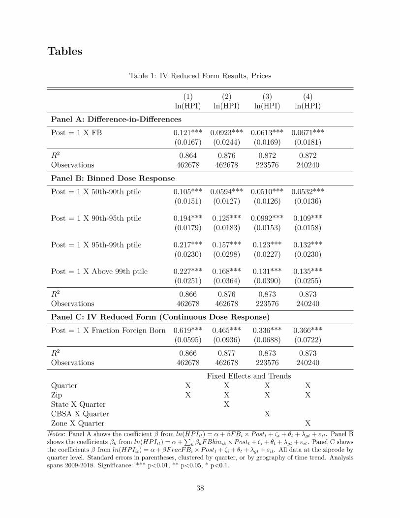
Tables

Table 1: IV Reduced Form Results, Prices

(1) (2) (3) (4)ln(HPI) ln(HPI) ln(HPI) ln(HPI)

Panel A: Difference-in-DifferencesPost = 1 X FB 0.121*** 0.0923*** 0.0613*** 0.0671***

(0.0167) (0.0244) (0.0169) (0.0181)R2 0.864 0.876 0.872 0.872Observations 462678 462678 223576 240240Panel B: Binned Dose ResponsePost = 1 X 50th-90th ptile 0.105*** 0.0594*** 0.0510*** 0.0532***

(0.0151) (0.0127) (0.0126) (0.0136)

Post = 1 X 90th-95th ptile 0.194*** 0.125*** 0.0992*** 0.109***(0.0179) (0.0183) (0.0153) (0.0158)

Post = 1 X 95th-99th ptile 0.217*** 0.157*** 0.123*** 0.132***(0.0230) (0.0298) (0.0227) (0.0230)

Post = 1 X Above 99th ptile 0.227*** 0.168*** 0.131*** 0.135***(0.0251) (0.0364) (0.0390) (0.0255)

R2 0.866 0.876 0.873 0.873Observations 462678 462678 223576 240240Panel C: IV Reduced Form (Continuous Dose Response)Post = 1 X Fraction Foreign Born 0.619*** 0.465*** 0.336*** 0.366***

(0.0595) (0.0936) (0.0688) (0.0722)R2 0.866 0.877 0.873 0.873Observations 462678 462678 223576 240240

Fixed Effects and TrendsQuarter X X X XZip X X X XState X Quarter XCBSA X Quarter XZone X Quarter X

Notes: Panel A shows the coefficient β from ln(HPIit) = α + βFBi × Postt + ζi + θt + λgt + εit. Panel Bshows the coefficients βk from ln(HPIit) = α+

∑k βkFBbinik × Postt + ζi + θt + λgt + εit. Panel C shows

the coefficients β from ln(HPIit) = α+ βFracFBi × Postt + ζi + θt + λgt + εit. All data at the zipcode byquarter level. Standard errors in parentheses, clustered by quarter, or by geography of time trend. Analysisspans 2009-2018. Significance: *** p<0.01, ** p<0.05, * p<0.1.

38

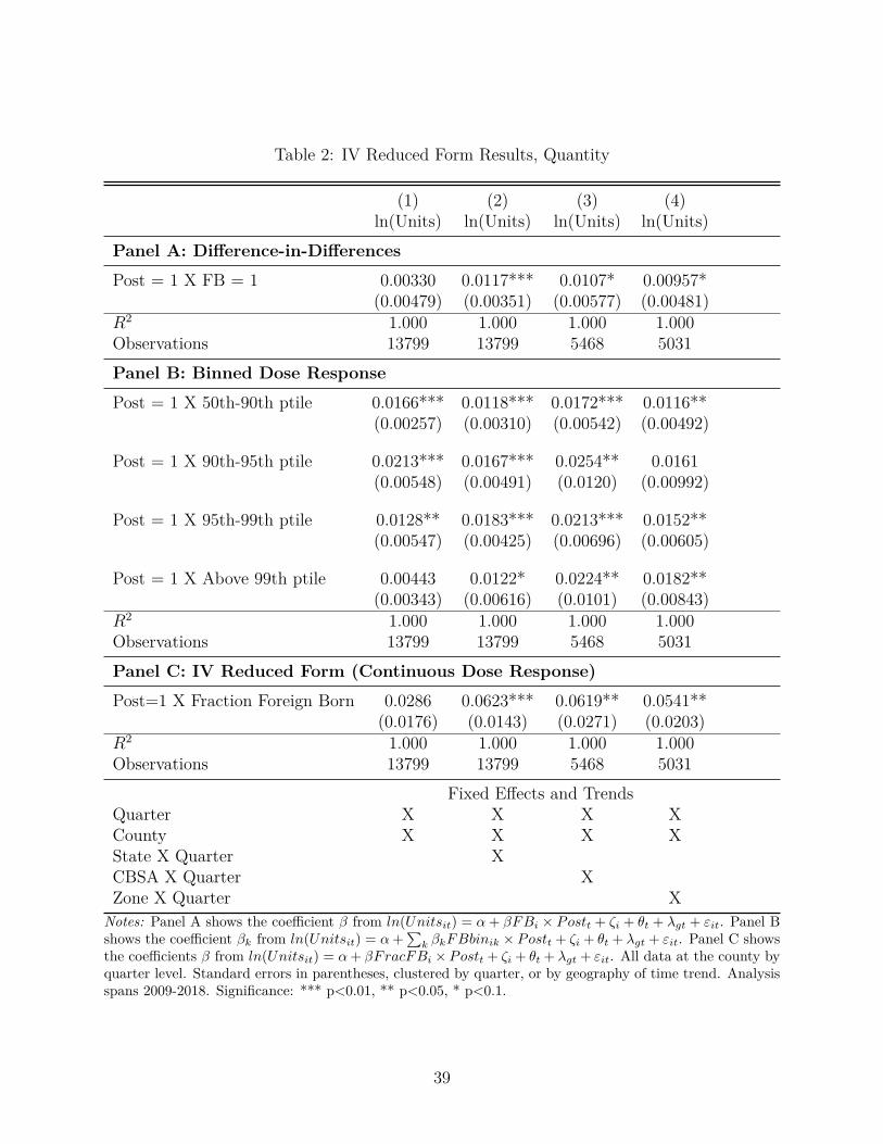
Table 2: IV Reduced Form Results, Quantity

(1) (2) (3) (4)ln(Units) ln(Units) ln(Units) ln(Units)

Panel A: Difference-in-DifferencesPost = 1 X FB = 1 0.00330 0.0117*** 0.0107* 0.00957*

(0.00479) (0.00351) (0.00577) (0.00481)R2 1.000 1.000 1.000 1.000Observations 13799 13799 5468 5031Panel B: Binned Dose ResponsePost = 1 X 50th-90th ptile 0.0166*** 0.0118*** 0.0172*** 0.0116**

(0.00257) (0.00310) (0.00542) (0.00492)

Post = 1 X 90th-95th ptile 0.0213*** 0.0167*** 0.0254** 0.0161(0.00548) (0.00491) (0.0120) (0.00992)

Post = 1 X 95th-99th ptile 0.0128** 0.0183*** 0.0213*** 0.0152**(0.00547) (0.00425) (0.00696) (0.00605)

Post = 1 X Above 99th ptile 0.00443 0.0122* 0.0224** 0.0182**(0.00343) (0.00616) (0.0101) (0.00843)

R2 1.000 1.000 1.000 1.000Observations 13799 13799 5468 5031Panel C: IV Reduced Form (Continuous Dose Response)Post=1 X Fraction Foreign Born 0.0286 0.0623*** 0.0619** 0.0541**

(0.0176) (0.0143) (0.0271) (0.0203)R2 1.000 1.000 1.000 1.000Observations 13799 13799 5468 5031

Fixed Effects and TrendsQuarter X X X XCounty X X X XState X Quarter XCBSA X Quarter XZone X Quarter X

Notes: Panel A shows the coefficient β from ln(Unitsit) = α+ βFBi × Postt + ζi + θt + λgt + εit. Panel Bshows the coefficient βk from ln(Unitsit) = α+

∑k βkFBbinik × Postt + ζi + θt + λgt + εit. Panel C shows

the coefficients β from ln(Unitsit) = α+ βFracFBi × Postt + ζi + θt + λgt + εit. All data at the county byquarter level. Standard errors in parentheses, clustered by quarter, or by geography of time trend. Analysisspans 2009-2018. Significance: *** p<0.01, ** p<0.05, * p<0.1.

39

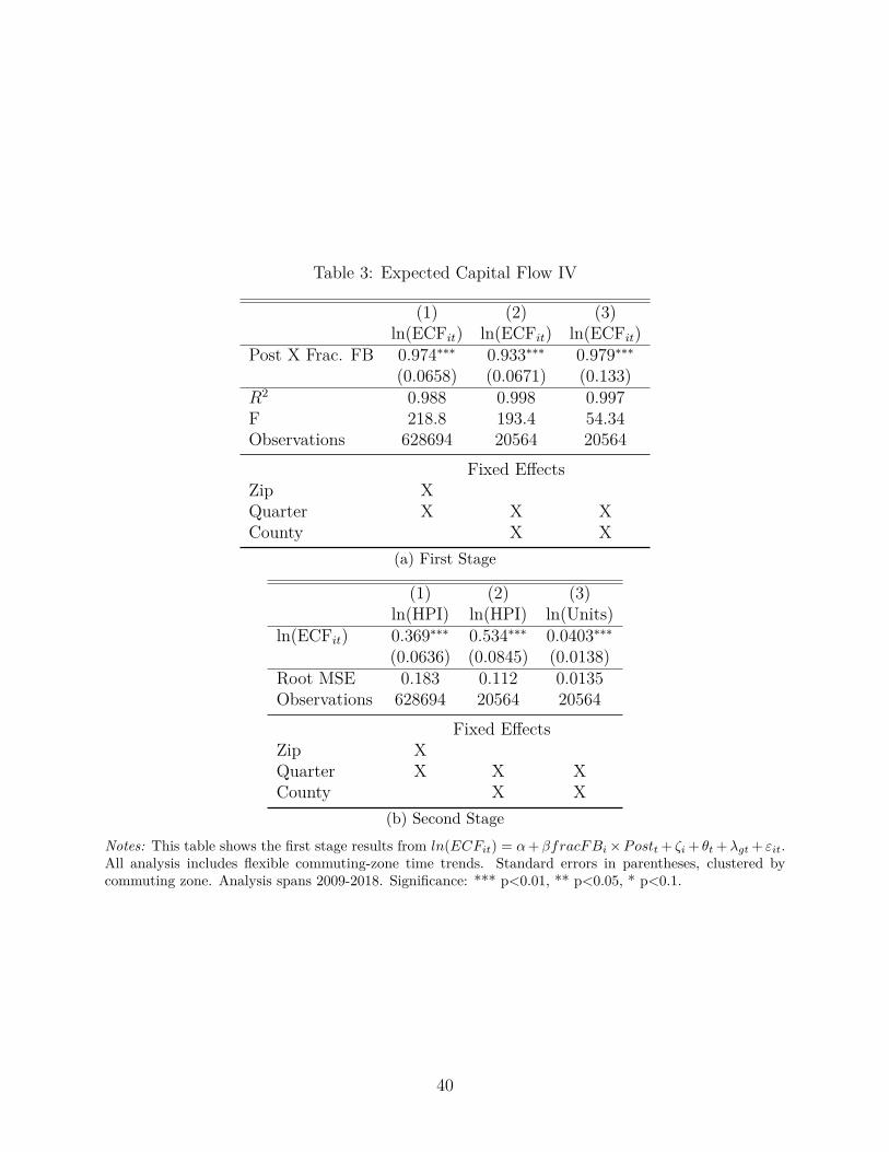
Table 3: Expected Capital Flow IV

(1) (2) (3)ln(ECFit) ln(ECFit) ln(ECFit)

Post X Frac. FB 0.974∗∗∗ 0.933∗∗∗ 0.979∗∗∗(0.0658) (0.0671) (0.133)

R2 0.988 0.998 0.997F 218.8 193.4 54.34Observations 628694 20564 20564

Fixed EffectsZip XQuarter X X XCounty X X

(a) First Stage

(1) (2) (3)ln(HPI) ln(HPI) ln(Units)

ln(ECFit) 0.369∗∗∗ 0.534∗∗∗ 0.0403∗∗∗(0.0636) (0.0845) (0.0138)

Root MSE 0.183 0.112 0.0135Observations 628694 20564 20564

Fixed EffectsZip XQuarter X X XCounty X X

(b) Second StageNotes: This table shows the first stage results from ln(ECFit) = α+βfracFBi×Postt + ζi + θt +λgt + εit.All analysis includes flexible commuting-zone time trends. Standard errors in parentheses, clustered bycommuting zone. Analysis spans 2009-2018. Significance: *** p<0.01, ** p<0.05, * p<0.1.

40

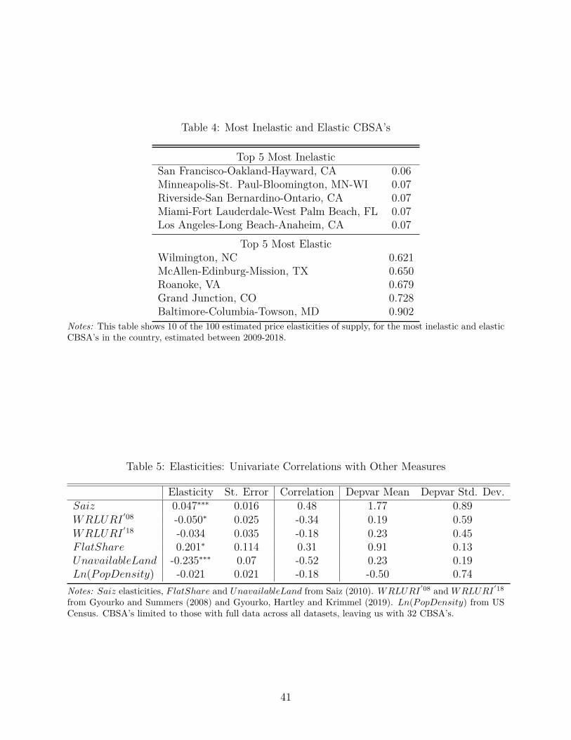
Table 4: Most Inelastic and Elastic CBSA’s

Top 5 Most InelasticSan Francisco-Oakland-Hayward, CA 0.06Minneapolis-St. Paul-Bloomington, MN-WI 0.07Riverside-San Bernardino-Ontario, CA 0.07Miami-Fort Lauderdale-West Palm Beach, FL 0.07Los Angeles-Long Beach-Anaheim, CA 0.07

Top 5 Most ElasticWilmington, NC 0.621McAllen-Edinburg-Mission, TX 0.650Roanoke, VA 0.679Grand Junction, CO 0.728Baltimore-Columbia-Towson, MD 0.902

Notes: This table shows 10 of the 100 estimated price elasticities of supply, for the most inelastic and elasticCBSA’s in the country, estimated between 2009-2018.

Table 5: Elasticities: Univariate Correlations with Other Measures

Elasticity St. Error Correlation Depvar Mean Depvar Std. Dev.Saiz 0.047∗∗∗ 0.016 0.48 1.77 0.89WRLURI

′08 -0.050∗ 0.025 -0.34 0.19 0.59WRLURI

′18 -0.034 0.035 -0.18 0.23 0.45FlatShare 0.201∗ 0.114 0.31 0.91 0.13UnavailableLand -0.235∗∗∗ 0.07 -0.52 0.23 0.19Ln(PopDensity) -0.021 0.021 -0.18 -0.50 0.74

Notes: Saiz elasticities, FlatShare and UnavailableLand from Saiz (2010). WRLURI′08 andWRLURI

′18

from Gyourko and Summers (2008) and Gyourko, Hartley and Krimmel (2019). Ln(PopDensity) from USCensus. CBSA’s limited to those with full data across all datasets, leaving us with 32 CBSA’s.

41

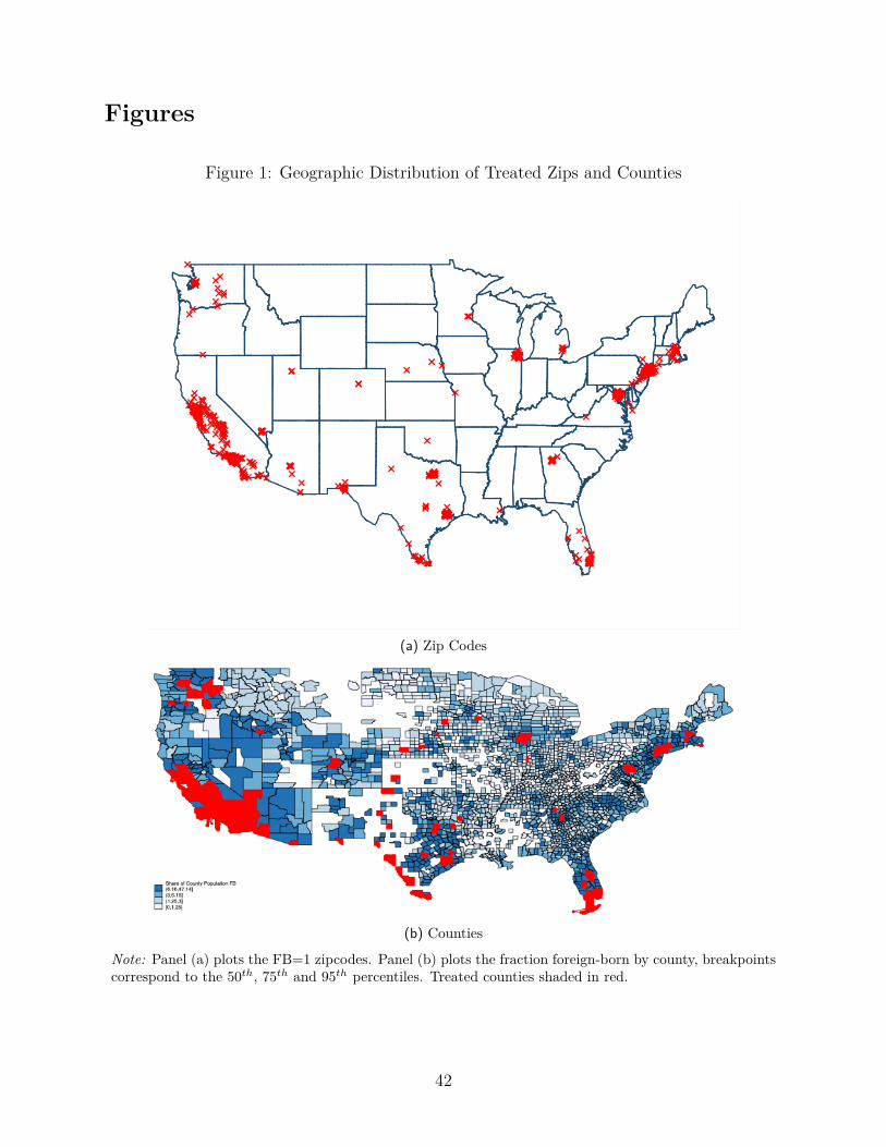
Figures

Figure 1: Geographic Distribution of Treated Zips and Counties

(a) Zip Codes

(b) Counties

Note: Panel (a) plots the FB=1 zipcodes. Panel (b) plots the fraction foreign-born by county, breakpointscorrespond to the 50th, 75th and 95th percentiles. Treated counties shaded in red.

42

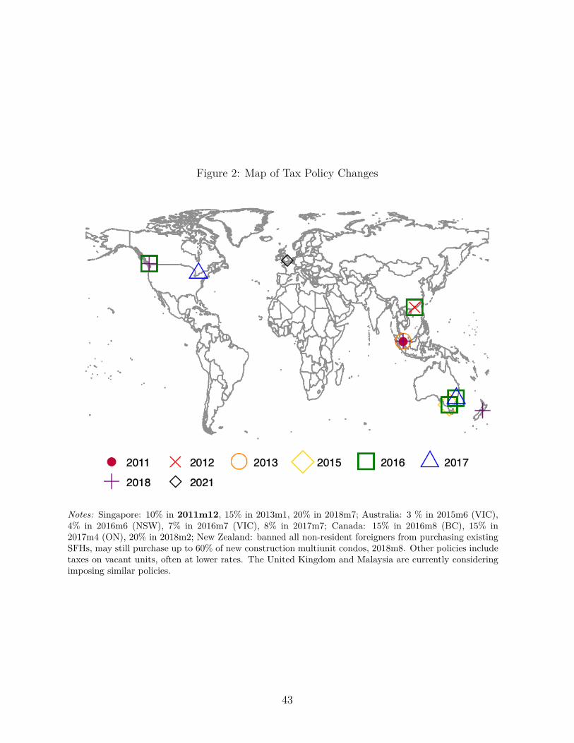
Figure 2: Map of Tax Policy Changes

Notes: Singapore: 10% in 2011m12, 15% in 2013m1, 20% in 2018m7; Australia: 3 % in 2015m6 (VIC),4% in 2016m6 (NSW), 7% in 2016m7 (VIC), 8% in 2017m7; Canada: 15% in 2016m8 (BC), 15% in2017m4 (ON), 20% in 2018m2; New Zealand: banned all non-resident foreigners from purchasing existingSFHs, may still purchase up to 60% of new construction multiunit condos, 2018m8. Other policies includetaxes on vacant units, often at lower rates. The United Kingdom and Malaysia are currently consideringimposing similar policies.

43

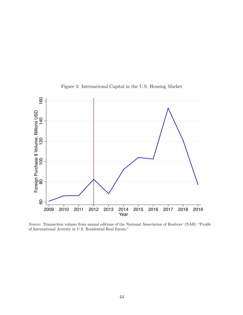
Figure 3: International Capital in the U.S. Housing Market

1st Foreign-Buyer Tax

6080

100

120

140

160

Fore

ign

Purc

hase

$ V

olum

e, B

illion

s U

SD

2009 2010 2011 2012 2013 2014 2015 2016 2017 2018 2019Year

Source: Transaction volume from annual editions of the National Association of Realtors’ (NAR) “Profileof International Activity in U.S. Residential Real Estate.”

44

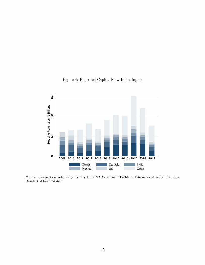
Figure 4: Expected Capital Flow Index Inputs

050

100

150

Hous

ing

Purc

hase

s, $

Billi

ons

2009 2010 2011 2012 2013 2014 2015 2016 2017 2018 2019

China Canada IndiaMexico UK Other

Source: Transaction volume by country from NAR’s annual “Profile of International Activity in U.S.Residential Real Estate.”

45

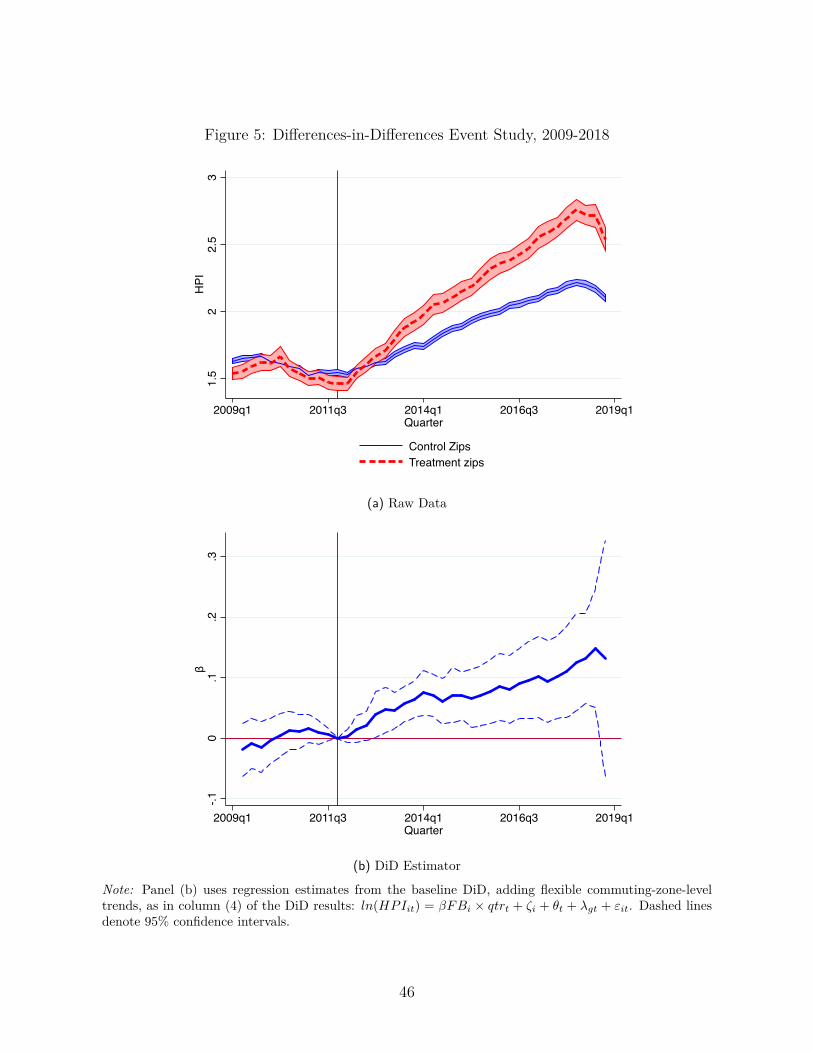
Figure 5: Differences-in-Differences Event Study, 2009-2018

1.5

22.

53

HPI

2009q1 2011q3 2014q1 2016q3 2019q1Quarter

Control ZipsTreatment zips

(a) Raw Data

-.10

.1.2

.3β

2009q1 2011q3 2014q1 2016q3 2019q1Quarter

(b) DiD Estimator

Note: Panel (b) uses regression estimates from the baseline DiD, adding flexible commuting-zone-leveltrends, as in column (4) of the DiD results: ln(HPIit) = βFBi × qtrt + ζi + θt + λgt + εit. Dashed linesdenote 95% confidence intervals.

46

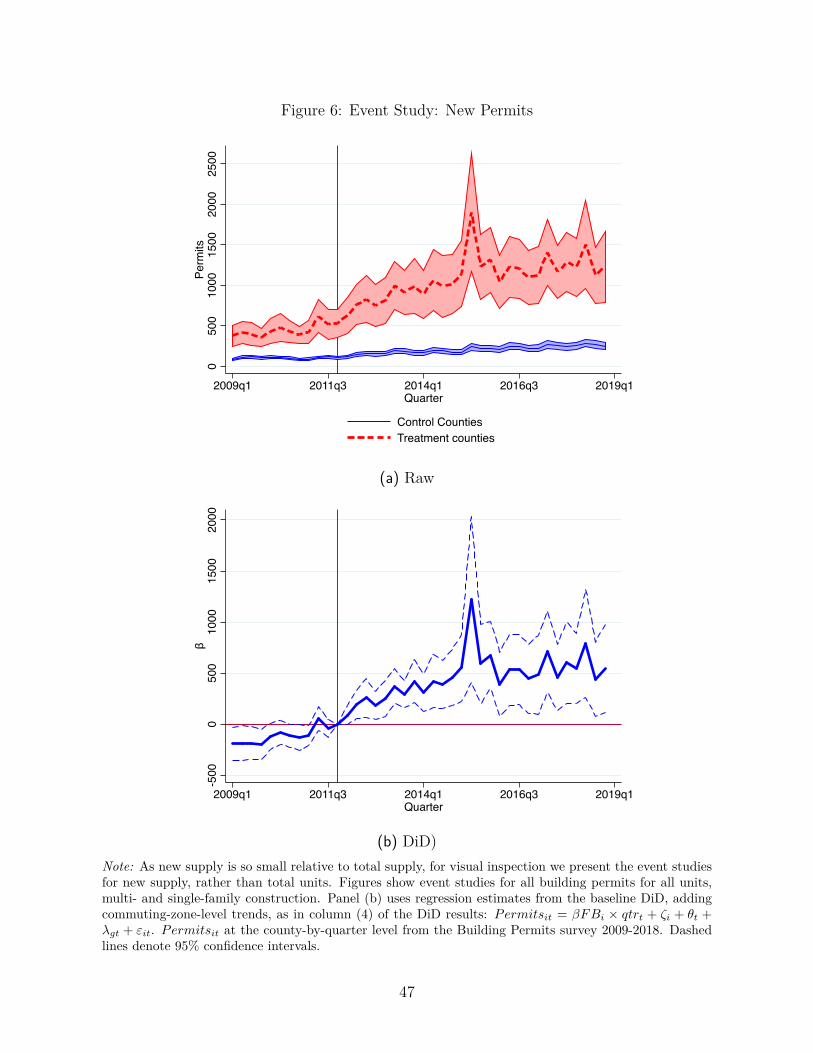
Figure 6: Event Study: New Permits

050

010

0015

0020

0025

00Pe

rmits

2009q1 2011q3 2014q1 2016q3 2019q1Quarter

Control CountiesTreatment counties

(a) Raw

-500

0500

1000

1500

2000

β

2009q1 2011q3 2014q1 2016q3 2019q1Quarter

(b) DiD)Note: As new supply is so small relative to total supply, for visual inspection we present the event studiesfor new supply, rather than total units. Figures show event studies for all building permits for all units,multi- and single-family construction. Panel (b) uses regression estimates from the baseline DiD, addingcommuting-zone-level trends, as in column (4) of the DiD results: Permitsit = βFBi × qtrt + ζi + θt +λgt + εit. Permitsit at the county-by-quarter level from the Building Permits survey 2009-2018. Dashedlines denote 95% confidence intervals.

47

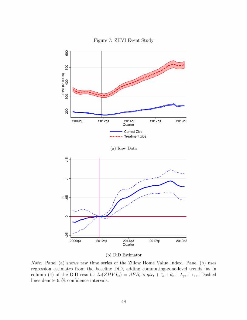
Figure 7: ZHVI Event Study

200

300

400

500

600

ZHVI

($10

00's)

2009q3 2012q1 2014q3 2017q1 2019q3Quarter

Control ZipsTreatment zips

(a) Raw Data

-.05

0.05

.1.15

β

2009q3 2012q1 2014q3 2017q1 2019q3Quarter

(b) DiD Estimator

Note: Panel (a) shows raw time series of the Zillow Home Value Index. Panel (b) usesregression estimates from the baseline DiD, adding commuting-zone-level trends, as incolumn (4) of the DiD results: ln(ZHV Iit) = βFBi × qtrt + ζi + θt + λgt + εit. Dashedlines denote 95% confidence intervals.

48

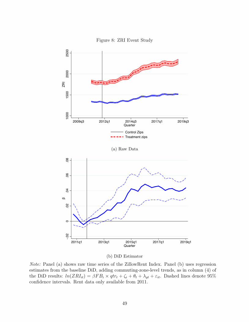
Figure 8: ZRI Event Study

1000

1500

2000

2500

ZRI

2009q3 2012q1 2014q3 2017q1 2019q3Quarter

Control ZipsTreatment zips

(a) Raw Data

-.02

0.02

.04

.06

.08

β

2011q1 2013q1 2015q1 2017q1 2019q1Quarter

(b) DiD Estimator

Note: Panel (a) shows raw time series of the ZillowRent Index. Panel (b) uses regressionestimates from the baseline DiD, adding commuting-zone-level trends, as in column (4) ofthe DiD results: ln(ZRIit) = βFBi × qtrt + ζi + θt + λgt + εit. Dashed lines denote 95%confidence intervals. Rent data only available from 2011.

49

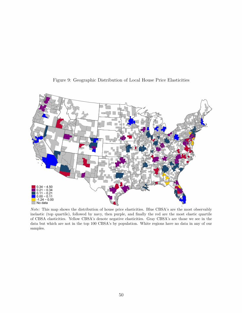
Figure 9: Geographic Distribution of Local House Price Elasticities

0.34 − 4.500.21 − 0.340.11 − 0.210.00 − 0.11-1.24 − 0.00No data

Note: This map shows the distribution of house price elasticities. Blue CBSA’s are the most observablyinelastic (top quartile), followed by navy, then purple, and finally the red are the most elastic quartileof CBSA elasticities. Yellow CBSA’s denote negative elasticities. Gray CBSA’s are those we see in thedata but which are not in the top 100 CBSA’s by population. White regions have no data in any of oursamples.

50

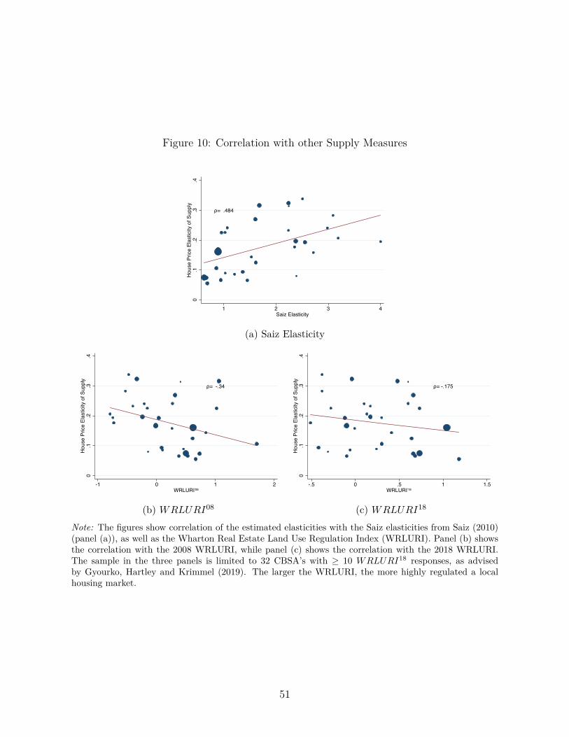
Figure 10: Correlation with other Supply Measures

ρ= .484

0.1

.2.3

.4H

ouse

Pric

e El

astic

ity o

f Sup

ply

1 2 3 4Saiz Elasticity

(a) Saiz Elasticity

ρ= -.34

0.1

.2.3

.4H

ouse

Pric

e El

astic

ity o

f Sup

ply

-1 0 1 2WRLURI'08

(b) WRLURI08

ρ= -.175

0.1

.2.3

.4H

ouse

Pric

e El

astic

ity o

f Sup

ply

-.5 0 .5 1 1.5WRLURI'18

(c) WRLURI18

Note: The figures show correlation of the estimated elasticities with the Saiz elasticities from Saiz (2010)(panel (a)), as well as the Wharton Real Estate Land Use Regulation Index (WRLURI). Panel (b) showsthe correlation with the 2008 WRLURI, while panel (c) shows the correlation with the 2018 WRLURI.The sample in the three panels is limited to 32 CBSA’s with ≥ 10 WRLURI18 responses, as advisedby Gyourko, Hartley and Krimmel (2019). The larger the WRLURI, the more highly regulated a localhousing market.

51

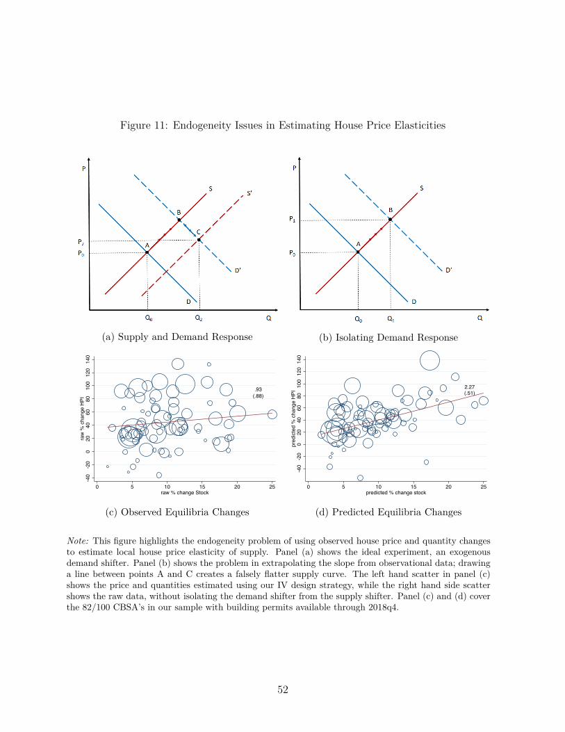
Figure 11: Endogeneity Issues in Estimating House Price Elasticities

(a) Supply and Demand Response (b) Isolating Demand Response

.93(.88)

-40

-20

020

4060

8010

012

014

0ra

w %

cha

nge

HPI

0 5 10 15 20 25raw % change Stock

(c) Observed Equilibria Changes

2.27(.51)

-40

-20

020

4060

8010

012

014

0pr

edic

ted

% c

hang

e H

PI

0 5 10 15 20 25predicted % change stock

(d) Predicted Equilibria Changes

Note: This figure highlights the endogeneity problem of using observed house price and quantity changesto estimate local house price elasticity of supply. Panel (a) shows the ideal experiment, an exogenousdemand shifter. Panel (b) shows the problem in extrapolating the slope from observational data; drawinga line between points A and C creates a falsely flatter supply curve. The left hand scatter in panel (c)shows the price and quantities estimated using our IV design strategy, while the right hand side scattershows the raw data, without isolating the demand shifter from the supply shifter. Panel (c) and (d) coverthe 82/100 CBSA’s in our sample with building permits available through 2018q4.

52

A Tax Policy Appendix

We have identified 10 policy events across five countries that make the U.S. housing marketrelatively cheaper to invest in from 2011 to 2018, as summarized in Figure 2. In response tosharply rising house prices, Singapore initiated the first tax on foreign buyers in December2011. All foreigners and entities (buyers who are not individuals) were charged a 10%Additional Buyer’s Stamp Duty (ABSD) on top of the Buyer’s Stamp Duty levied on all realestate purchases. In January 2013, Singapore raised the ABSD to 15% for foreigners andentities, and introduced an ABSD of 5% on Singapore Permanent Residents. The ABSDincreased again in July 2018 to 20% for foreigners, 25% for entities, and 30% for housingdevelopers.

Hong Kong introduced a 15% buyer stamp duty (BSD) for non-residents in October 2012.Under the policy, any buyer who was not a Hong Kong permanent resident paid the tax ontop of their purchase price. The policy extended to include companies buying properties,regardless of their local or nonlocal status. In addition to the purchase tax, Hong Kongraised the special transactions tax, which is levied on housing sales that occur within threeyears of initial purchase, from 10% to 20% to discourage speculation in the housing market.In November 2016, the Hong Kong government raised the stamp duty for all non first-timeresidential property buyers, applicable to both residents and non-residents, from 8.5% to15%. This effectively raised the taxes paid by foreign parties from 23.5% to 30%.

The state of Victoria, Australia (home to Melbourne) introduced the Foreign PurchaserAdditional Duty, applicable to foreign persons, corporations, and trusts purchasing residen-tial property (or non-residential property with the intent of conversion) in June 2015. Anadditional duty at 3% of the dutiable value (the higher of the price paid for the property orthe market value) was imposed from June 2015 to July 2016. It was subsequently raised to7% in July 2016. In June 2016, the state of New South Wales, Australia (home to Sydney)introduced a 4% surcharge purchaser duty (SPD) applicable to residential real estate pur-chases by foreign persons. The state raised the SPD to 8% in July 2017. All duties are paidon top of the original duties paid by any purchaser of residential real estate.

The provincial government of British Columbia, Canada (home to Vancouver) passedBill 28 in August 2016, which introduced a foreign-buyer tax, as well as a vacancy tax tospecific communities in B.C. From August 2016 until February 2018, foreign buyers in theGreater Vancouver Regional District paid an additional 15% of the fair market value in tax.In February 2018, the tax amount increased to 20% of the fair market value and expandedgeographically. At the same time, the city of Vancouver initiated a vacant homes tax of 1%of the assessed taxable value on residences not occupied for at least 6 months of the year.

53

Ontario, Canada’s provincial government implemented the Non-Resident SpeculationTax (NRST) in April 2017. As per NRST, foreign entities pay a 15% tax on the residentialproperty value for any property located in the Greater Golden Horseshoe Region of Ontario,which covers approximately 1/5th of the population of Canada (and includes Toronto).

Most dramatically, in August 2018, New Zealand barred non-residents from purchasingreal estate, excepting Singaporeans and Australians due to existing trade agreements. Anumber of national and local governments continue to tighten restrictions for foreign buyers.In October 2018, Theresa May announced plans to implement a foreign buyer tax in theUnited Kingdom, and Governor Andrew Cuomo included a pied-à-terre tax in his proposed2019 New York State budget. In July 2018, the Chief Executive of Hong Kong suggestedshe was open to further policies aimed at limiting non-resident housing purchases.

Figure E1 documents the effects of these foreign-buyer taxes on their respective localmarkets; all graphs plot house price indexes, and include sales volume when available. Forinstance, Figure E1d displays one of the more recent policy interventions in British Columbia,and the results in the local housing market. After the enactment of the taxes, the 12-monthsales volume moving average fell by 54% between its peak in February 2016 and March 2019.Although the tax has had little effect on the level of Vancouver housing prices, with the12-month moving average falling only 1%, house price growth has effectively ceased.

B IV Approach Appendix

B.1 Check of Exclusion Restriction Violation

A plausible violation of the exclusion restriction is that investment in the technology sectordrives house price results. As foreign countries impose foreign buyer taxes, foreigners couldchoose to invest in U.S. tech stocks instead of in foreign real estate. This would lead to eco-nomic growth in tech-heavy locations, which tend to be inelastically supplied with housing,increasing house prices. Therefore, the tax policy change =⇒ E[εit(fracFBi×Postt)] 6= 0,where Postt is the tax policy change, and the city’s high-tech status is in εit, which is thesecond stage error term, and thus correlated with the second stage left-hand-side variable,ln(HPIit).

We test for this mechanism by directly controlling for employment and establishmentchanges in the tech sector. Appendix Table D6 shows the results as in Table 1, but alsocontrolling for either employment or establishments, by NAICS category. Employment andestablishment data is taken at the county by year level from the County Business Patterns2009-2018, and so is both local and time-varying. The top panel controls for establishments

54

or employment in levels, while the bottom panel controls by share. We limit the sampleto those zipcodes in a commuting zone that has at least one foreign-born zipcode, as incolumn(4) of Table 1.

In both panels, the baseline point estimate shows that after the Singaporean foreign buyertax, zipcodes with high fractions of foreign-born residents see, on average, 7% higher HPIrelative to their peers in the same commuting zone. Adding controls from the number of firmsin the management and professional services industries, as in Ding et al. (2019), column (2)reports that the point estimate remains stable. Controlling just for “Professional, Scientific,and Technical Services” in column (3) yields a similar result. Column (4) controls for thenumber of businesses in “Computer Systems Design and Related Services,” with a similarpoint estimate. Columns (5) - (7) repeat the controls, but use time-varying employmentrather than establishment count.

Finally, we can remove tech-heavy housing markets from the data, and check whether themain results go through. Table D7 removes Seattle, WA, San Jose, CA and San Francisco,CA from our sample and reruns the main differences-in-differences analysis. The baselinepoint estimates from Table 1 suggested differential growth in foreign-born zipcodes of 6-9%,and the results in Table D7 show similar point estimates of 6-9%.

In sum, accounting for differential trends in the tech sector between 2009 and 2018 doesnot meaningfully alter our estimates of the impact of foreign capital flowing to U.S. housingmarkets, and specifically to zipcodes with ex-ante high shares of foreign-born residents.

B.2 Expected Capital Flows, Exposure IV

The ECF ′it exposure IV scales the per-capita capital flows by the fraction foreign-born of therespective country within a zipcode. For example, consider two zipcodes with 3 foreign-bornresidents. In the baseline ECFit, each foeign-born resident receives the same per-capitashare of the national capital flow from their origin country into the U.S. housing market.The exposure index scales this per-capita share by the share of foreign-born residents in thetotal population of the zipcode. If the first zipcode has 10 residents, and the second has 100,then the first zipcode is therefore more exposed to the foreign capital as it is diluted amongfewer non-foreign-born residents:

ECF ′it =∑c∈C

capflowct ×FBpop2011

ic

FBpop2011c

fracFBic (12)

55

where

1 =∑i

FBpop2011ic

FBpop2011c

(13)

and C = {Canada, China, India, Mexico, United Kingdom, Other}, i denotes zipcode, t de-notes quarter.

Appendix Table D10 shows the results using the exposure ECF ′it. The second stageyields a price elasticity estimate of 0.54 for the zipcode panel and 0.875 for the county panel,larger but in the same ballpark as our preferred estimates, while the coefficient on units issimilar to the main results.

56

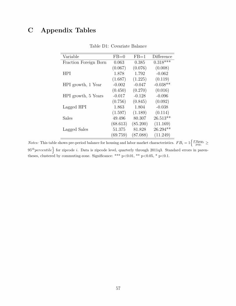
C Appendix Tables

Table D1: Covariate Balance

Variable FB=0 FB=1 DifferenceFraction Foreign Born 0.063 0.385 0.318***

(0.067) (0.076) (0.008)HPI 1.878 1.792 -0.062

(1.687) (1.225) (0.119)HPI growth, 1 Year -0.002 -0.047 -0.038**

(0.450) (0.270) (0.016)HPI growth, 5 Years -0.017 -0.128 -0.096

(0.756) (0.845) (0.092)Lagged HPI 1.863 1.804 -0.038

(1.597) (1.189) (0.114)Sales 49.496 80.307 26.513**

(68.613) (85.200) (11.169)Lagged Sales 51.375 81.828 26.294**

(69.759) (87.088) (11.249)Notes: This table shows pre-period balance for housing and labor market characteristics. FBi = 1

{F Bpopi

popi≥

95thpercentile}

for zipcode i. Data is zipcode level, quarterly through 2011q3. Standard errors in paren-theses, clustered by commuting-zone. Significance: *** p<0.01, ** p<0.05, * p<0.1.

57

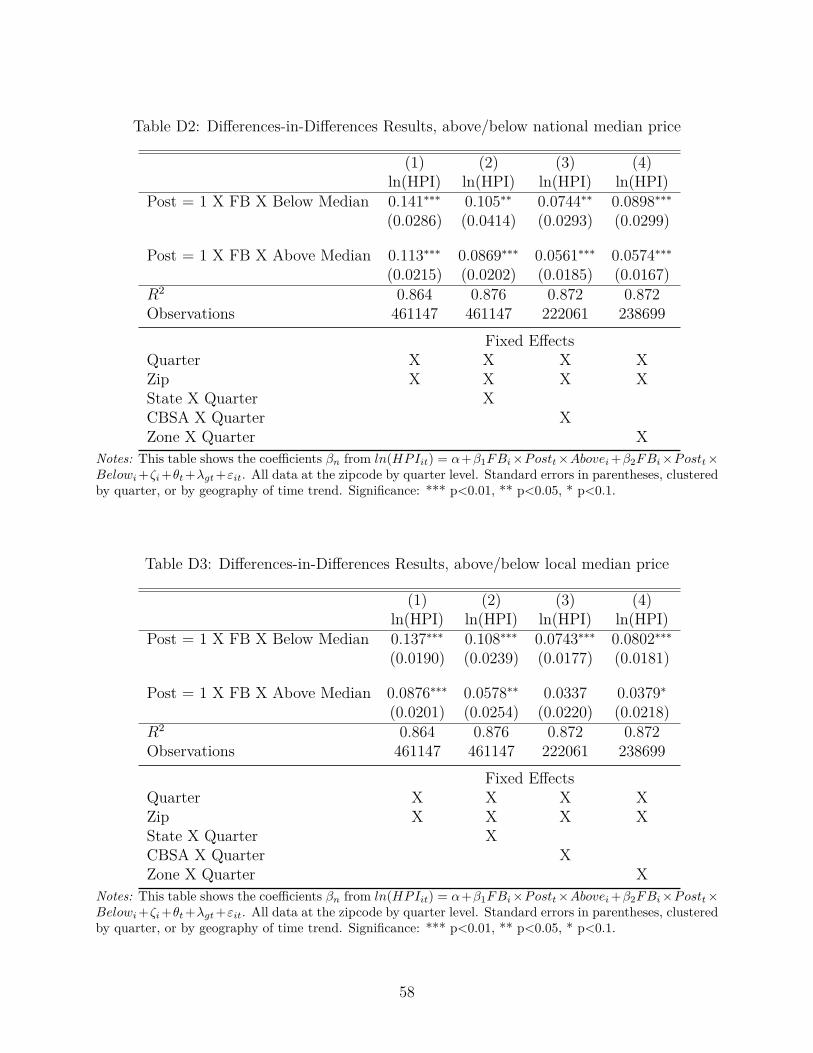
Table D2: Differences-in-Differences Results, above/below national median price

(1) (2) (3) (4)ln(HPI) ln(HPI) ln(HPI) ln(HPI)

Post = 1 X FB X Below Median 0.141∗∗∗ 0.105∗∗ 0.0744∗∗ 0.0898∗∗∗(0.0286) (0.0414) (0.0293) (0.0299)

Post = 1 X FB X Above Median 0.113∗∗∗ 0.0869∗∗∗ 0.0561∗∗∗ 0.0574∗∗∗(0.0215) (0.0202) (0.0185) (0.0167)

R2 0.864 0.876 0.872 0.872Observations 461147 461147 222061 238699

Fixed EffectsQuarter X X X XZip X X X XState X Quarter XCBSA X Quarter XZone X Quarter X

Notes: This table shows the coefficients βn from ln(HPIit) = α+β1FBi×Postt×Abovei +β2FBi×Postt×Belowi +ζi +θt +λgt +εit. All data at the zipcode by quarter level. Standard errors in parentheses, clusteredby quarter, or by geography of time trend. Significance: *** p<0.01, ** p<0.05, * p<0.1.

Table D3: Differences-in-Differences Results, above/below local median price

(1) (2) (3) (4)ln(HPI) ln(HPI) ln(HPI) ln(HPI)

Post = 1 X FB X Below Median 0.137∗∗∗ 0.108∗∗∗ 0.0743∗∗∗ 0.0802∗∗∗(0.0190) (0.0239) (0.0177) (0.0181)

Post = 1 X FB X Above Median 0.0876∗∗∗ 0.0578∗∗ 0.0337 0.0379∗(0.0201) (0.0254) (0.0220) (0.0218)

R2 0.864 0.876 0.872 0.872Observations 461147 461147 222061 238699

Fixed EffectsQuarter X X X XZip X X X XState X Quarter XCBSA X Quarter XZone X Quarter X

Notes: This table shows the coefficients βn from ln(HPIit) = α+β1FBi×Postt×Abovei +β2FBi×Postt×Belowi +ζi +θt +λgt +εit. All data at the zipcode by quarter level. Standard errors in parentheses, clusteredby quarter, or by geography of time trend. Significance: *** p<0.01, ** p<0.05, * p<0.1.

58

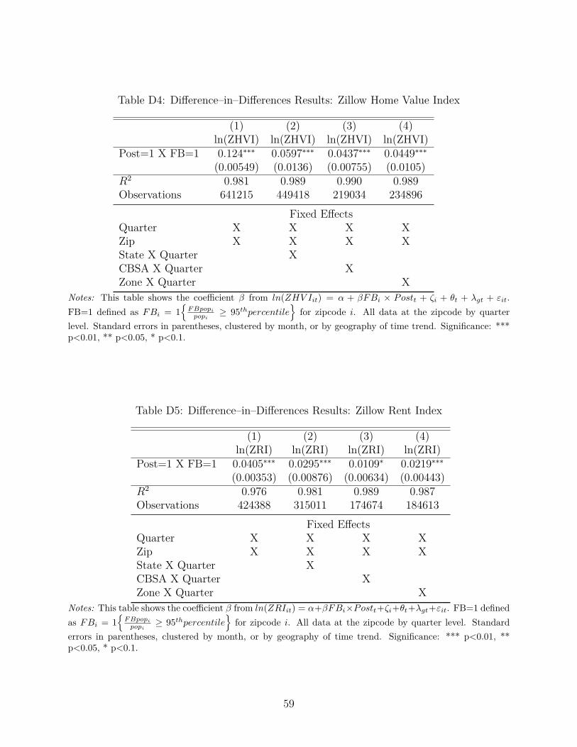
Table D4: Difference–in–Differences Results: Zillow Home Value Index

(1) (2) (3) (4)ln(ZHVI) ln(ZHVI) ln(ZHVI) ln(ZHVI)

Post=1 X FB=1 0.124∗∗∗ 0.0597∗∗∗ 0.0437∗∗∗ 0.0449∗∗∗(0.00549) (0.0136) (0.00755) (0.0105)

R2 0.981 0.989 0.990 0.989Observations 641215 449418 219034 234896

Fixed EffectsQuarter X X X XZip X X X XState X Quarter XCBSA X Quarter XZone X Quarter X

Notes: This table shows the coefficient β from ln(ZHV Iit) = α + βFBi × Postt + ζi + θt + λgt + εit.FB=1 defined as FBi = 1

{F Bpopi

popi≥ 95thpercentile

}for zipcode i. All data at the zipcode by quarter

level. Standard errors in parentheses, clustered by month, or by geography of time trend. Significance: ***p<0.01, ** p<0.05, * p<0.1.

Table D5: Difference–in–Differences Results: Zillow Rent Index

(1) (2) (3) (4)ln(ZRI) ln(ZRI) ln(ZRI) ln(ZRI)

Post=1 X FB=1 0.0405∗∗∗ 0.0295∗∗∗ 0.0109∗ 0.0219∗∗∗(0.00353) (0.00876) (0.00634) (0.00443)

R2 0.976 0.981 0.989 0.987Observations 424388 315011 174674 184613

Fixed EffectsQuarter X X X XZip X X X XState X Quarter XCBSA X Quarter XZone X Quarter X

Notes: This table shows the coefficient β from ln(ZRIit) = α+βFBi×Postt+ζi+θt+λgt+εit. FB=1 definedas FBi = 1

{F Bpopi

popi≥ 95thpercentile

}for zipcode i. All data at the zipcode by quarter level. Standard

errors in parentheses, clustered by month, or by geography of time trend. Significance: *** p<0.01, **p<0.05, * p<0.1.

59

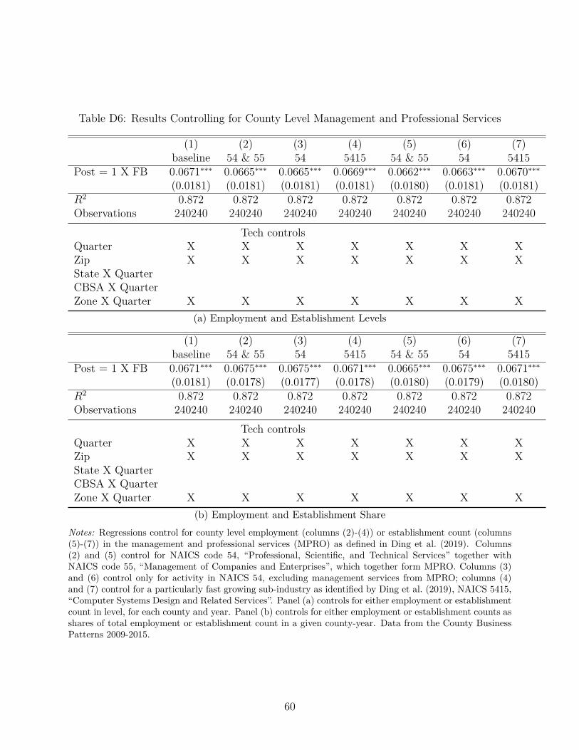
Table D6: Results Controlling for County Level Management and Professional Services

(1) (2) (3) (4) (5) (6) (7)baseline 54 & 55 54 5415 54 & 55 54 5415

Post = 1 X FB 0.0671∗∗∗ 0.0665∗∗∗ 0.0665∗∗∗ 0.0669∗∗∗ 0.0662∗∗∗ 0.0663∗∗∗ 0.0670∗∗∗(0.0181) (0.0181) (0.0181) (0.0181) (0.0180) (0.0181) (0.0181)

R2 0.872 0.872 0.872 0.872 0.872 0.872 0.872Observations 240240 240240 240240 240240 240240 240240 240240

Tech controlsQuarter X X X X X X XZip X X X X X X XState X QuarterCBSA X QuarterZone X Quarter X X X X X X X

(a) Employment and Establishment Levels

(1) (2) (3) (4) (5) (6) (7)baseline 54 & 55 54 5415 54 & 55 54 5415

Post = 1 X FB 0.0671∗∗∗ 0.0675∗∗∗ 0.0675∗∗∗ 0.0671∗∗∗ 0.0665∗∗∗ 0.0675∗∗∗ 0.0671∗∗∗(0.0181) (0.0178) (0.0177) (0.0178) (0.0180) (0.0179) (0.0180)

R2 0.872 0.872 0.872 0.872 0.872 0.872 0.872Observations 240240 240240 240240 240240 240240 240240 240240

Tech controlsQuarter X X X X X X XZip X X X X X X XState X QuarterCBSA X QuarterZone X Quarter X X X X X X X

(b) Employment and Establishment ShareNotes: Regressions control for county level employment (columns (2)-(4)) or establishment count (columns(5)-(7)) in the management and professional services (MPRO) as defined in Ding et al. (2019). Columns(2) and (5) control for NAICS code 54, “Professional, Scientific, and Technical Services” together withNAICS code 55, “Management of Companies and Enterprises”, which together form MPRO. Columns (3)and (6) control only for activity in NAICS 54, excluding management services from MPRO; columns (4)and (7) control for a particularly fast growing sub-industry as identified by Ding et al. (2019), NAICS 5415,“Computer Systems Design and Related Services”. Panel (a) controls for either employment or establishmentcount in level, for each county and year. Panel (b) controls for either employment or establishment counts asshares of total employment or establishment count in a given county-year. Data from the County BusinessPatterns 2009-2015.

60

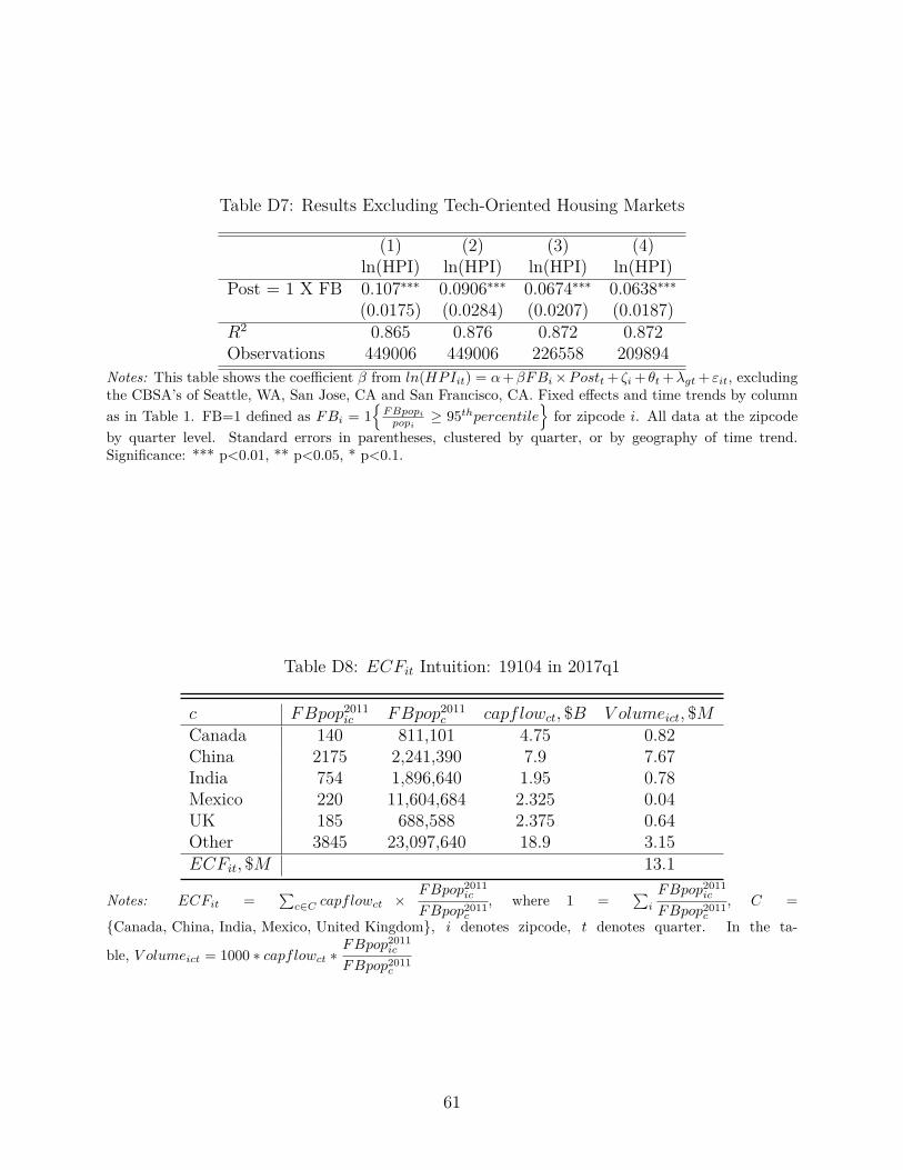
Table D7: Results Excluding Tech-Oriented Housing Markets

(1) (2) (3) (4)ln(HPI) ln(HPI) ln(HPI) ln(HPI)

Post = 1 X FB 0.107∗∗∗ 0.0906∗∗∗ 0.0674∗∗∗ 0.0638∗∗∗(0.0175) (0.0284) (0.0207) (0.0187)

R2 0.865 0.876 0.872 0.872Observations 449006 449006 226558 209894

Notes: This table shows the coefficient β from ln(HPIit) = α+βFBi×Postt + ζi + θt +λgt + εit, excludingthe CBSA’s of Seattle, WA, San Jose, CA and San Francisco, CA. Fixed effects and time trends by columnas in Table 1. FB=1 defined as FBi = 1

{F Bpopi

popi≥ 95thpercentile

}for zipcode i. All data at the zipcode

by quarter level. Standard errors in parentheses, clustered by quarter, or by geography of time trend.Significance: *** p<0.01, ** p<0.05, * p<0.1.

Table D8: ECFit Intuition: 19104 in 2017q1

c FBpop2011ic FBpop2011

c capflowct, $B V olumeict, $MCanada 140 811,101 4.75 0.82China 2175 2,241,390 7.9 7.67India 754 1,896,640 1.95 0.78Mexico 220 11,604,684 2.325 0.04UK 185 688,588 2.375 0.64Other 3845 23,097,640 18.9 3.15ECFit, $M 13.1

Notes: ECFit =∑

c∈C capflowct ×FBpop2011

ic

FBpop2011c

, where 1 =∑

i

FBpop2011ic

FBpop2011c

, C =

{Canada, China, India, Mexico, United Kingdom}, i denotes zipcode, t denotes quarter. In the ta-

ble, V olumeict = 1000 ∗ capflowct ∗FBpop2011

ic

FBpop2011c

61

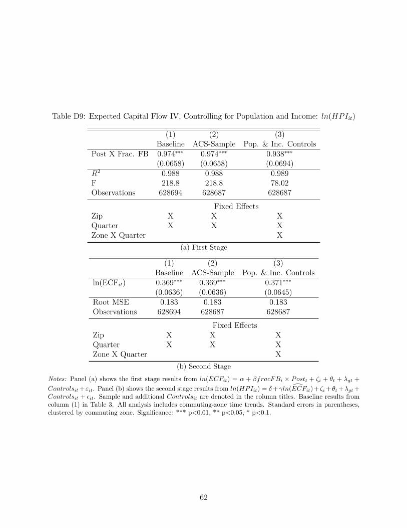
Table D9: Expected Capital Flow IV, Controlling for Population and Income: ln(HPIit)

(1) (2) (3)Baseline ACS-Sample Pop. & Inc. Controls

Post X Frac. FB 0.974∗∗∗ 0.974∗∗∗ 0.938∗∗∗(0.0658) (0.0658) (0.0694)

R2 0.988 0.988 0.989F 218.8 218.8 78.02Observations 628694 628687 628687

Fixed EffectsZip X X XQuarter X X XZone X Quarter X

(a) First Stage

(1) (2) (3)Baseline ACS-Sample Pop. & Inc. Controls

ln(ECFit) 0.369∗∗∗ 0.369∗∗∗ 0.371∗∗∗(0.0636) (0.0636) (0.0645)

Root MSE 0.183 0.183 0.183Observations 628694 628687 628687

Fixed EffectsZip X X XQuarter X X XZone X Quarter X

(b) Second StageNotes: Panel (a) shows the first stage results from ln(ECFit) = α + βfracFBi × Postt + ζi + θt + λgt +Controlsit +εit. Panel (b) shows the second stage results from ln(HPIit) = δ+γ ln(ECFit)+ ζi +θt +λgt +Controlsit + εit. Sample and additional Controlsit are denoted in the column titles. Baseline results fromcolumn (1) in Table 3. All analysis includes commuting-zone time trends. Standard errors in parentheses,clustered by commuting zone. Significance: *** p<0.01, ** p<0.05, * p<0.1.

62

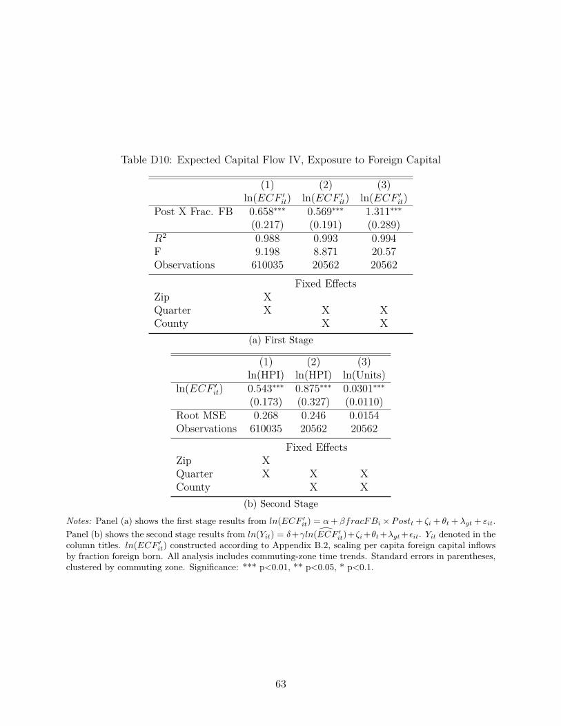
Table D10: Expected Capital Flow IV, Exposure to Foreign Capital

(1) (2) (3)ln(ECF ′it) ln(ECF ′it) ln(ECF ′it)

Post X Frac. FB 0.658∗∗∗ 0.569∗∗∗ 1.311∗∗∗(0.217) (0.191) (0.289)

R2 0.988 0.993 0.994F 9.198 8.871 20.57Observations 610035 20562 20562

Fixed EffectsZip XQuarter X X XCounty X X

(a) First Stage

(1) (2) (3)ln(HPI) ln(HPI) ln(Units)

ln(ECF ′it) 0.543∗∗∗ 0.875∗∗∗ 0.0301∗∗∗(0.173) (0.327) (0.0110)

Root MSE 0.268 0.246 0.0154Observations 610035 20562 20562

Fixed EffectsZip XQuarter X X XCounty X X

(b) Second StageNotes: Panel (a) shows the first stage results from ln(ECF ′

it) = α+ βfracFBi ×Postt + ζi + θt + λgt + εit.Panel (b) shows the second stage results from ln(Yit) = δ+γ ln(ECF ′

it)+ζi +θt +λgt +εit. Yit denoted in thecolumn titles. ln(ECF ′

it) constructed according to Appendix B.2, scaling per capita foreign capital inflowsby fraction foreign born. All analysis includes commuting-zone time trends. Standard errors in parentheses,clustered by commuting zone. Significance: *** p<0.01, ** p<0.05, * p<0.1.

63

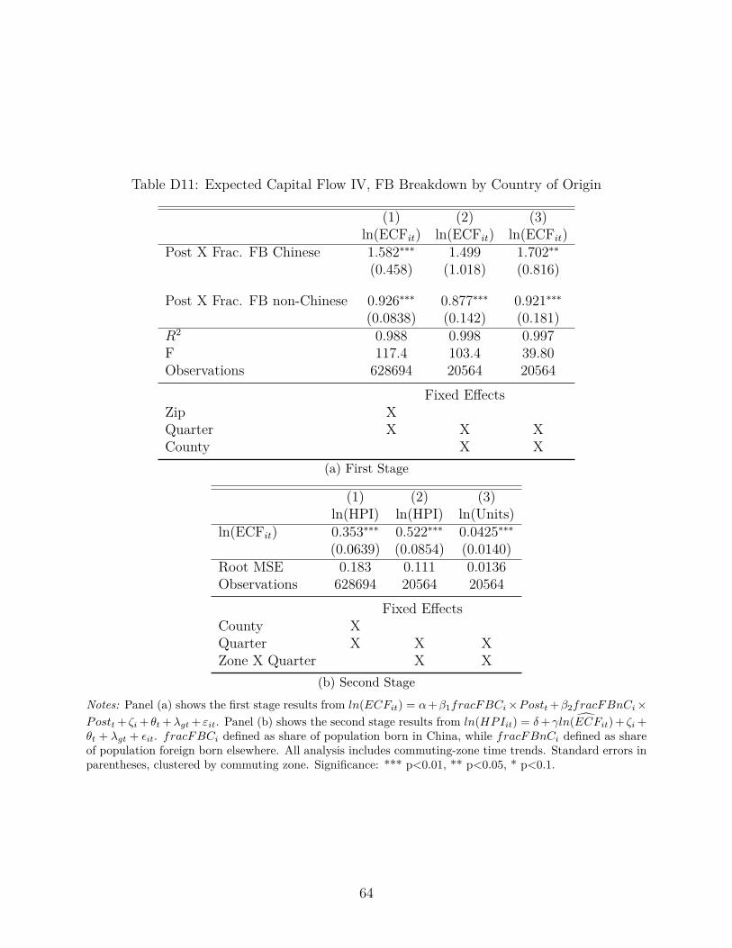
Table D11: Expected Capital Flow IV, FB Breakdown by Country of Origin

(1) (2) (3)ln(ECFit) ln(ECFit) ln(ECFit)

Post X Frac. FB Chinese 1.582∗∗∗ 1.499 1.702∗∗(0.458) (1.018) (0.816)

Post X Frac. FB non-Chinese 0.926∗∗∗ 0.877∗∗∗ 0.921∗∗∗(0.0838) (0.142) (0.181)

R2 0.988 0.998 0.997F 117.4 103.4 39.80Observations 628694 20564 20564

Fixed EffectsZip XQuarter X X XCounty X X

(a) First Stage

(1) (2) (3)ln(HPI) ln(HPI) ln(Units)

ln(ECFit) 0.353∗∗∗ 0.522∗∗∗ 0.0425∗∗∗(0.0639) (0.0854) (0.0140)

Root MSE 0.183 0.111 0.0136Observations 628694 20564 20564

Fixed EffectsCounty XQuarter X X XZone X Quarter X X

(b) Second StageNotes: Panel (a) shows the first stage results from ln(ECFit) = α+β1fracFBCi×Postt +β2fracFBnCi×Postt + ζi + θt +λgt + εit. Panel (b) shows the second stage results from ln(HPIit) = δ+ γ ln(ECFit) + ζi +θt + λgt + εit. fracFBCi defined as share of population born in China, while fracFBnCi defined as shareof population foreign born elsewhere. All analysis includes commuting-zone time trends. Standard errors inparentheses, clustered by commuting zone. Significance: *** p<0.01, ** p<0.05, * p<0.1.

64

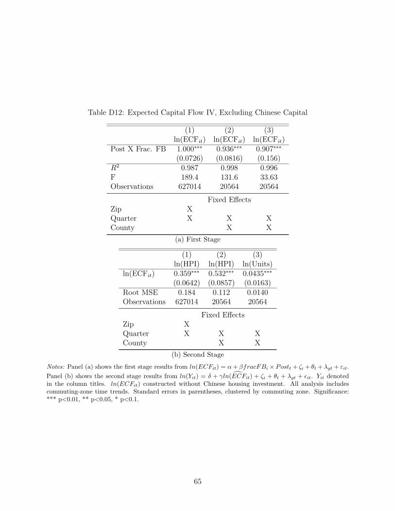
Table D12: Expected Capital Flow IV, Excluding Chinese Capital

(1) (2) (3)ln(ECFit) ln(ECFit) ln(ECFit)

Post X Frac. FB 1.000∗∗∗ 0.936∗∗∗ 0.907∗∗∗(0.0726) (0.0816) (0.156)

R2 0.987 0.998 0.996F 189.4 131.6 33.63Observations 627014 20564 20564

Fixed EffectsZip XQuarter X X XCounty X X

(a) First Stage

(1) (2) (3)ln(HPI) ln(HPI) ln(Units)

ln(ECFit) 0.359∗∗∗ 0.532∗∗∗ 0.0435∗∗∗(0.0642) (0.0857) (0.0163)

Root MSE 0.184 0.112 0.0140Observations 627014 20564 20564

Fixed EffectsZip XQuarter X X XCounty X X

(b) Second StageNotes: Panel (a) shows the first stage results from ln(ECFit) = α+ βfracFBi ×Postt + ζi + θt + λgt + εit.Panel (b) shows the second stage results from ln(Yit) = δ + γ ln(ECFit) + ζi + θt + λgt + εit. Yit denotedin the column titles. ln(ECFit) constructed without Chinese housing investment. All analysis includescommuting-zone time trends. Standard errors in parentheses, clustered by commuting zone. Significance:*** p<0.01, ** p<0.05, * p<0.1.

65

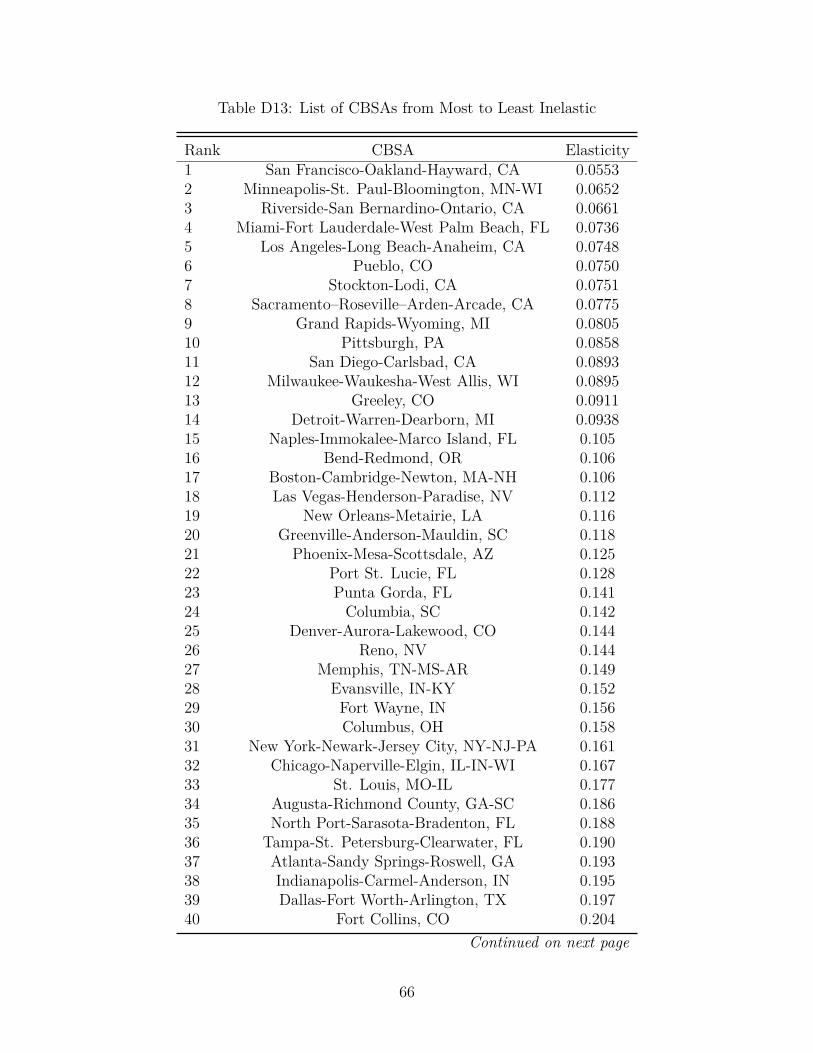
Table D13: List of CBSAs from Most to Least Inelastic

Rank CBSA Elasticity1 San Francisco-Oakland-Hayward, CA 0.05532 Minneapolis-St. Paul-Bloomington, MN-WI 0.06523 Riverside-San Bernardino-Ontario, CA 0.06614 Miami-Fort Lauderdale-West Palm Beach, FL 0.07365 Los Angeles-Long Beach-Anaheim, CA 0.07486 Pueblo, CO 0.07507 Stockton-Lodi, CA 0.07518 Sacramento–Roseville–Arden-Arcade, CA 0.07759 Grand Rapids-Wyoming, MI 0.080510 Pittsburgh, PA 0.085811 San Diego-Carlsbad, CA 0.089312 Milwaukee-Waukesha-West Allis, WI 0.089513 Greeley, CO 0.091114 Detroit-Warren-Dearborn, MI 0.093815 Naples-Immokalee-Marco Island, FL 0.10516 Bend-Redmond, OR 0.10617 Boston-Cambridge-Newton, MA-NH 0.10618 Las Vegas-Henderson-Paradise, NV 0.11219 New Orleans-Metairie, LA 0.11620 Greenville-Anderson-Mauldin, SC 0.11821 Phoenix-Mesa-Scottsdale, AZ 0.12522 Port St. Lucie, FL 0.12823 Punta Gorda, FL 0.14124 Columbia, SC 0.14225 Denver-Aurora-Lakewood, CO 0.14426 Reno, NV 0.14427 Memphis, TN-MS-AR 0.14928 Evansville, IN-KY 0.15229 Fort Wayne, IN 0.15630 Columbus, OH 0.15831 New York-Newark-Jersey City, NY-NJ-PA 0.16132 Chicago-Naperville-Elgin, IL-IN-WI 0.16733 St. Louis, MO-IL 0.17734 Augusta-Richmond County, GA-SC 0.18635 North Port-Sarasota-Bradenton, FL 0.18836 Tampa-St. Petersburg-Clearwater, FL 0.19037 Atlanta-Sandy Springs-Roswell, GA 0.19338 Indianapolis-Carmel-Anderson, IN 0.19539 Dallas-Fort Worth-Arlington, TX 0.19740 Fort Collins, CO 0.204

Continued on next page

66

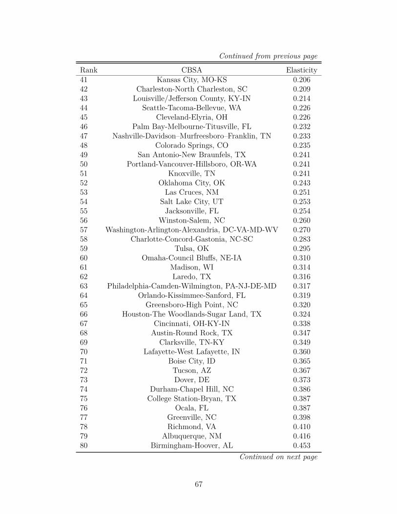
Continued from previous page

Rank CBSA Elasticity41 Kansas City, MO-KS 0.20642 Charleston-North Charleston, SC 0.20943 Louisville/Jefferson County, KY-IN 0.21444 Seattle-Tacoma-Bellevue, WA 0.22645 Cleveland-Elyria, OH 0.22646 Palm Bay-Melbourne-Titusville, FL 0.23247 Nashville-Davidson–Murfreesboro–Franklin, TN 0.23348 Colorado Springs, CO 0.23549 San Antonio-New Braunfels, TX 0.24150 Portland-Vancouver-Hillsboro, OR-WA 0.24151 Knoxville, TN 0.24152 Oklahoma City, OK 0.24353 Las Cruces, NM 0.25154 Salt Lake City, UT 0.25355 Jacksonville, FL 0.25456 Winston-Salem, NC 0.26057 Washington-Arlington-Alexandria, DC-VA-MD-WV 0.27058 Charlotte-Concord-Gastonia, NC-SC 0.28359 Tulsa, OK 0.29560 Omaha-Council Bluffs, NE-IA 0.31061 Madison, WI 0.31462 Laredo, TX 0.31663 Philadelphia-Camden-Wilmington, PA-NJ-DE-MD 0.31764 Orlando-Kissimmee-Sanford, FL 0.31965 Greensboro-High Point, NC 0.32066 Houston-The Woodlands-Sugar Land, TX 0.32467 Cincinnati, OH-KY-IN 0.33868 Austin-Round Rock, TX 0.34769 Clarksville, TN-KY 0.34970 Lafayette-West Lafayette, IN 0.36071 Boise City, ID 0.36572 Tucson, AZ 0.36773 Dover, DE 0.37374 Durham-Chapel Hill, NC 0.38675 College Station-Bryan, TX 0.38776 Ocala, FL 0.38777 Greenville, NC 0.39878 Richmond, VA 0.41079 Albuquerque, NM 0.41680 Birmingham-Hoover, AL 0.453

Continued on next page

67

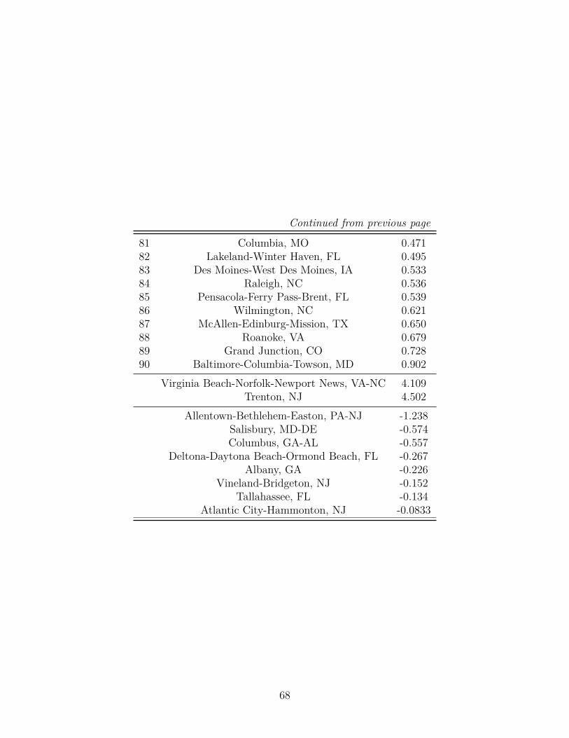
Continued from previous page

81 Columbia, MO 0.47182 Lakeland-Winter Haven, FL 0.49583 Des Moines-West Des Moines, IA 0.53384 Raleigh, NC 0.53685 Pensacola-Ferry Pass-Brent, FL 0.53986 Wilmington, NC 0.62187 McAllen-Edinburg-Mission, TX 0.65088 Roanoke, VA 0.67989 Grand Junction, CO 0.72890 Baltimore-Columbia-Towson, MD 0.902

Virginia Beach-Norfolk-Newport News, VA-NC 4.109Trenton, NJ 4.502

Allentown-Bethlehem-Easton, PA-NJ -1.238Salisbury, MD-DE -0.574Columbus, GA-AL -0.557

Deltona-Daytona Beach-Ormond Beach, FL -0.267Albany, GA -0.226

Vineland-Bridgeton, NJ -0.152Tallahassee, FL -0.134

Atlantic City-Hammonton, NJ -0.0833

68

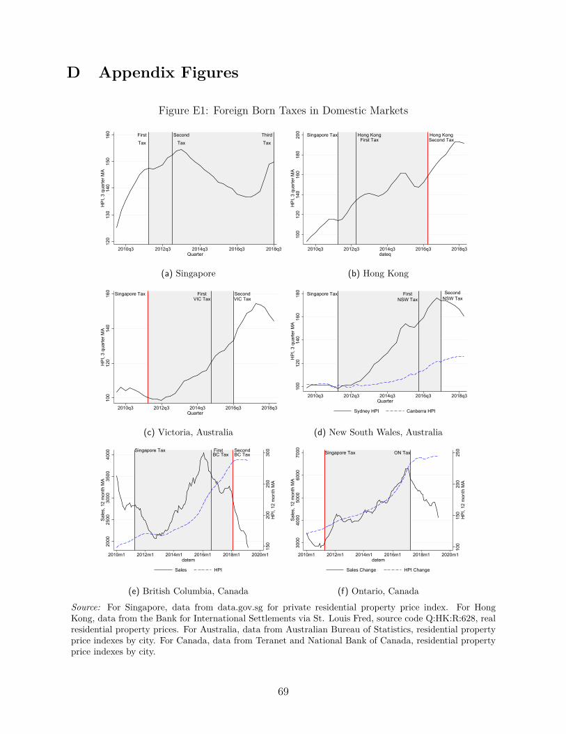
D Appendix Figures

Figure E1: Foreign Born Taxes in Domestic Markets

First

Tax

Second

Tax

Third

Tax

120

130

140

150

160

HP

I, 3

quar

ter M

A

2010q3 2012q3 2014q3 2016q3 2018q3Quarter

(a) Singapore

Singapore Tax Hong KongFirst Tax

Hong KongSecond Tax

100

120

140

160

180

200

HP

I, 3

quar

ter M

A

2010q3 2012q3 2014q3 2016q3 2018q3dateq

(b) Hong Kong

Singapore Tax FirstVIC Tax

SecondVIC Tax

100

120

140

160

HP

I, 3

quar

ter M

A

2010q3 2012q3 2014q3 2016q3 2018q3Quarter

(c) Victoria, Australia

Singapore Tax FirstNSW Tax

SecondNSW Tax

100

120

140

160

180

HP

I, 3

quar

ter M

A

2010q3 2012q3 2014q3 2016q3 2018q3Quarter

Sydney HPI Canberra HPI

(d) New South Wales, Australia

Singapore Tax FirstBC Tax

SecondBC Tax

150

200

250

300

HP

I, 12

mon

th M

A

2000

2500

3000

3500

4000

Sal

es, 1

2 m

onth

MA

2010m1 2012m1 2014m1 2016m1 2018m1 2020m1datem

Sales HPI

(e) British Columbia, Canada

Singapore Tax ON Tax10

015

020

025

0H

PI,

12 m

onth

MA

3000

4000

5000

6000

7000

Sal

es, 1

2 m

onth

MA

2010m1 2012m1 2014m1 2016m1 2018m1 2020m1datem

Sales Change HPI Change

(f) Ontario, Canada

Source: For Singapore, data from data.gov.sg for private residential property price index. For HongKong, data from the Bank for International Settlements via St. Louis Fred, source code Q:HK:R:628, realresidential property prices. For Australia, data from Australian Bureau of Statistics, residential propertyprice indexes by city. For Canada, data from Teranet and National Bank of Canada, residential propertyprice indexes by city.

69

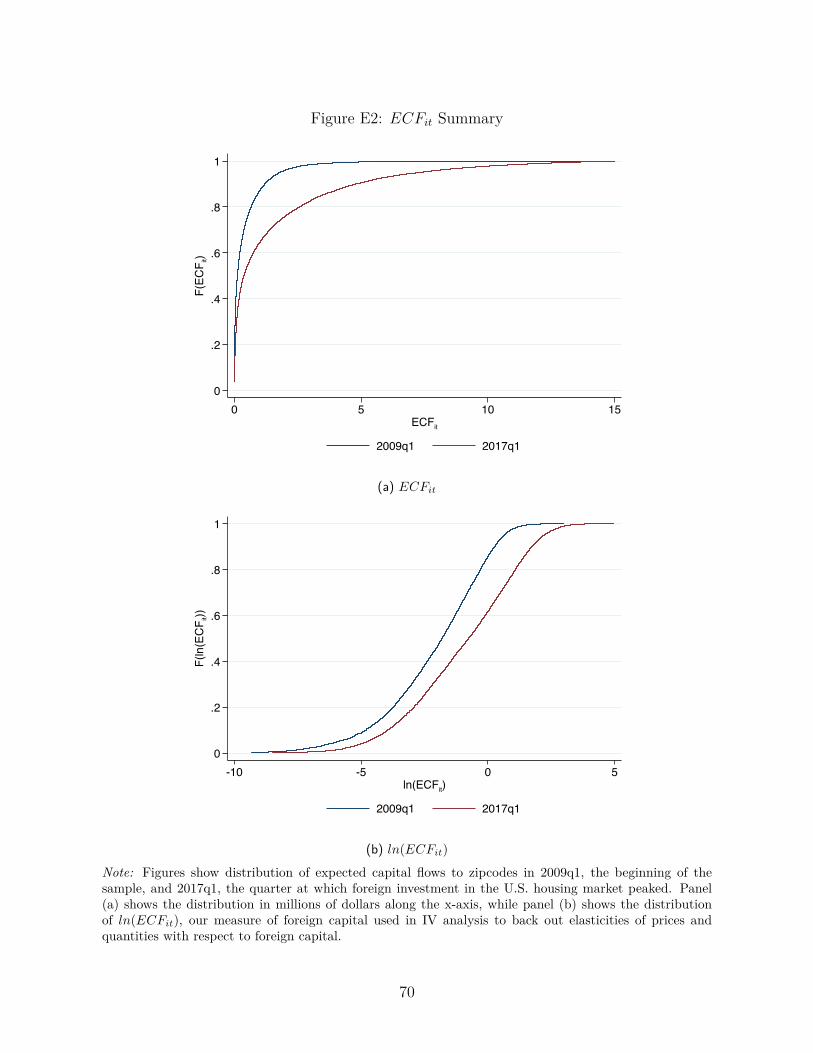
Figure E2: ECFit Summary

0

.2

.4

.6

.8

1

F(EC

F it)

0 5 10 15ECFit

2009q1 2017q1

(a) ECFit

0

.2

.4

.6

.8

1

F(ln(ECF i

t))

-10 -5 0 5ln(ECFit)

2009q1 2017q1

(b) ln(ECFit)

Note: Figures show distribution of expected capital flows to zipcodes in 2009q1, the beginning of thesample, and 2017q1, the quarter at which foreign investment in the U.S. housing market peaked. Panel(a) shows the distribution in millions of dollars along the x-axis, while panel (b) shows the distributionof ln(ECFit), our measure of foreign capital used in IV analysis to back out elasticities of prices andquantities with respect to foreign capital.

70