GIS ANALYSIS/ OPERATIONS 1. Interpolation based operations Interpolation is the procedure of estimating the value of properties at unsampled points or areas using a limited number of sampled observations. Interpolation Techniques Pointwise interpolation : Pointwise interpolation is used in case the sampled points are not densely located with a limited influence or continuity in surrounding observations, for example climate observations such as rainfall and temperature, or ground water level measurements at wells. 1(a) Thiessen polygon: Thiessen polygons can be generated using distance operator which creates the polygon boundaries as the intersections of radial expansions from the observation points. 1(b) Weighted Average : A window of circular shape with the radius of d max is drawn at a point to be interpolated, so as to involve six to eight surrounding observed points.

Welcome message from author
This document is posted to help you gain knowledge. Please leave a comment to let me know what you think about it! Share it to your friends and learn new things together.
Transcript
GIS ANALYSIS/ OPERATIONS
1. Interpolation based operations
Interpolation is the procedure of estimating the value of properties at unsampled points or areas
using a limited number of sampled observations.
Interpolation Techniques
Pointwise interpolation : Pointwise interpolation is used in case the sampled points are not
densely located with a limited influence or continuity in surrounding observations, for example
climate observations such as rainfall and temperature, or ground water level measurements at
wells.
1(a) Thiessen polygon: Thiessen polygons can be generated using distance operator which
creates the polygon boundaries as the intersections of radial expansions from the observation
points.
1(b) Weighted Average : A window of circular shape with the radius of dmax is drawn at a
point to be interpolated, so as to involve six to eight surrounding observed points.
hp
Highlight
hp
Highlight
hp
Highlight
hp
Highlight
hp
Highlight

1(c). INTERPOLATION by Inverse Distance Weighted (IDW)
1(d) Kriging
Similar to Inverse Distance Weighting (IDW), Kriging uses the minimum variance method to
calculate the weights rather than applying an arbitrary or less precise weighting scheme.
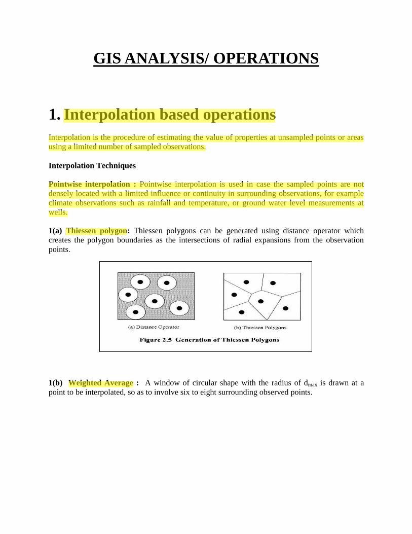
2. Interpolation by curve fitting: the principle of curve fitting respectively to interpolate the
value at an unsampled point using surrounding sampled points.
hp
Highlight
hp
Highlight
hp
Highlight
2.1 Exact interpolation: a fitted curve passes through all given points.
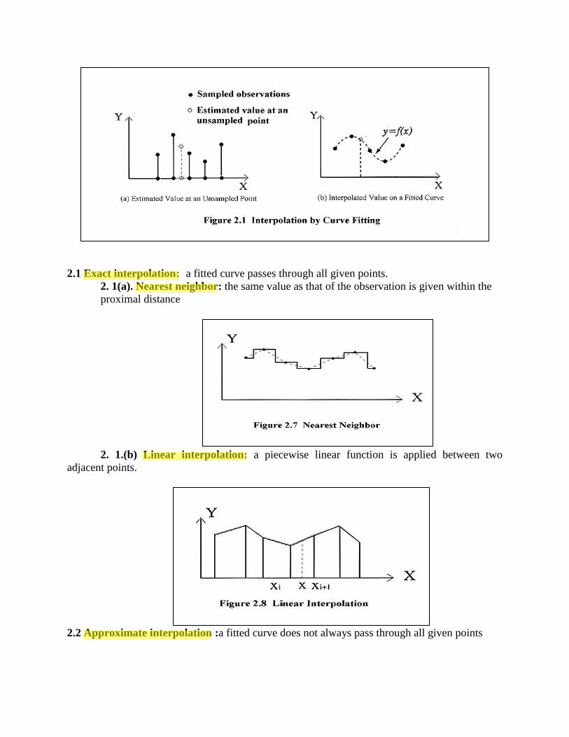
2. 1(a). Nearest neighbor: the same value as that of the observation is given within the
proximal distance
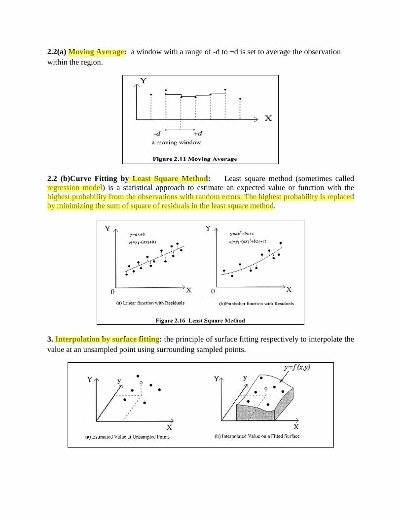
2. 1.(b) Linear interpolation: a piecewise linear function is applied between two
adjacent points.
2.2 Approximate interpolation :a fitted curve does not always pass through all given points
hp
Highlight
hp
Highlight
hp
Highlight
hp
Highlight
2.2(a) Moving Average: a window with a range of -d to +d is set to average the observation
within the region.
2.2 (b)Curve Fitting by Least Square Method: Least square method (sometimes called
regression model) is a statistical approach to estimate an expected value or function with the
highest probability from the observations with random errors. The highest probability is replaced
by minimizing the sum of square of residuals in the least square method.
3. Interpolation by surface fitting: the principle of surface fitting respectively to interpolate the
value at an unsampled point using surrounding sampled points.
hp
Highlight
hp
Highlight
hp
Highlight
hp
Highlight
hp
Highlight
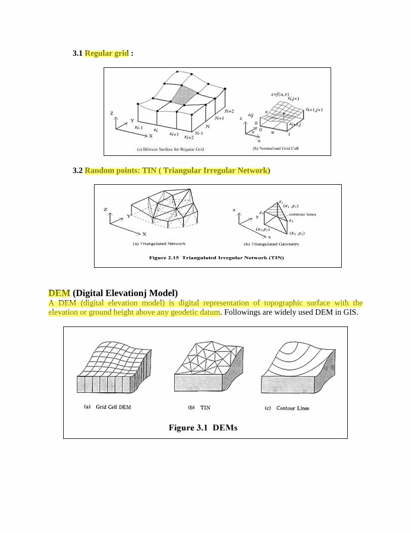
3.1 Regular grid :
3.2 Random points: TIN ( Triangular Irregular Network)
DEM (Digital Elevationj Model) A DEM (digital elevation model) is digital representation of topographic surface with the
elevation or ground height above any geodetic datum. Followings are widely used DEM in GIS.
hp
Highlight
hp
Highlight
hp
Highlight
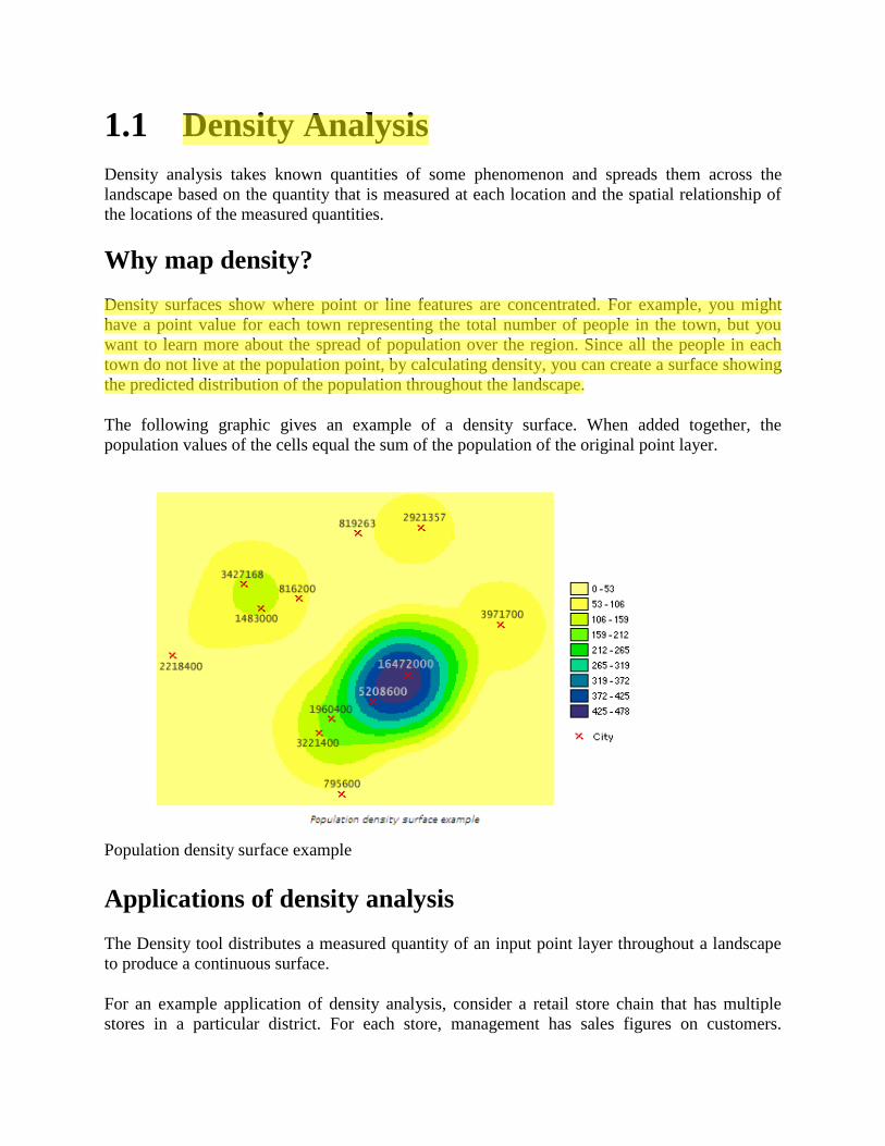
1.1 Density Analysis
Density analysis takes known quantities of some phenomenon and spreads them across the
landscape based on the quantity that is measured at each location and the spatial relationship of
the locations of the measured quantities.
Why map density?
Density surfaces show where point or line features are concentrated. For example, you might
have a point value for each town representing the total number of people in the town, but you
want to learn more about the spread of population over the region. Since all the people in each
town do not live at the population point, by calculating density, you can create a surface showing
the predicted distribution of the population throughout the landscape.
The following graphic gives an example of a density surface. When added together, the
population values of the cells equal the sum of the population of the original point layer.
Population density surface example
Applications of density analysis
The Density tool distributes a measured quantity of an input point layer throughout a landscape
to produce a continuous surface.
For an example application of density analysis, consider a retail store chain that has multiple
stores in a particular district. For each store, management has sales figures on customers.
hp
Highlight
Proximity analysis
hp
Highlight
Management assumes that customers patronize one store over another based on how far they
have to travel. In this example, it is natural to assume that any single customer will always
choose the closest store. The farther away from the closest store, the farther the customer will
need to travel to that store. But shoppers farther away may also shop at other stores. Management
wants to study the distribution of where the customers live. From the sales figures and the spatial
distribution of the stores, management wants to create a surface of customers by intelligently
spreading the customers out across the landscape.
To accomplish this task, the Density tool considers where each store is in relation to other stores,
the quantity of customers shopping at each store, and how many cells need to share a portion of
the measured quantity (the shoppers). The cells nearer the measured points, the stores, receive
higher proportions of the measured quantity than those farther away.
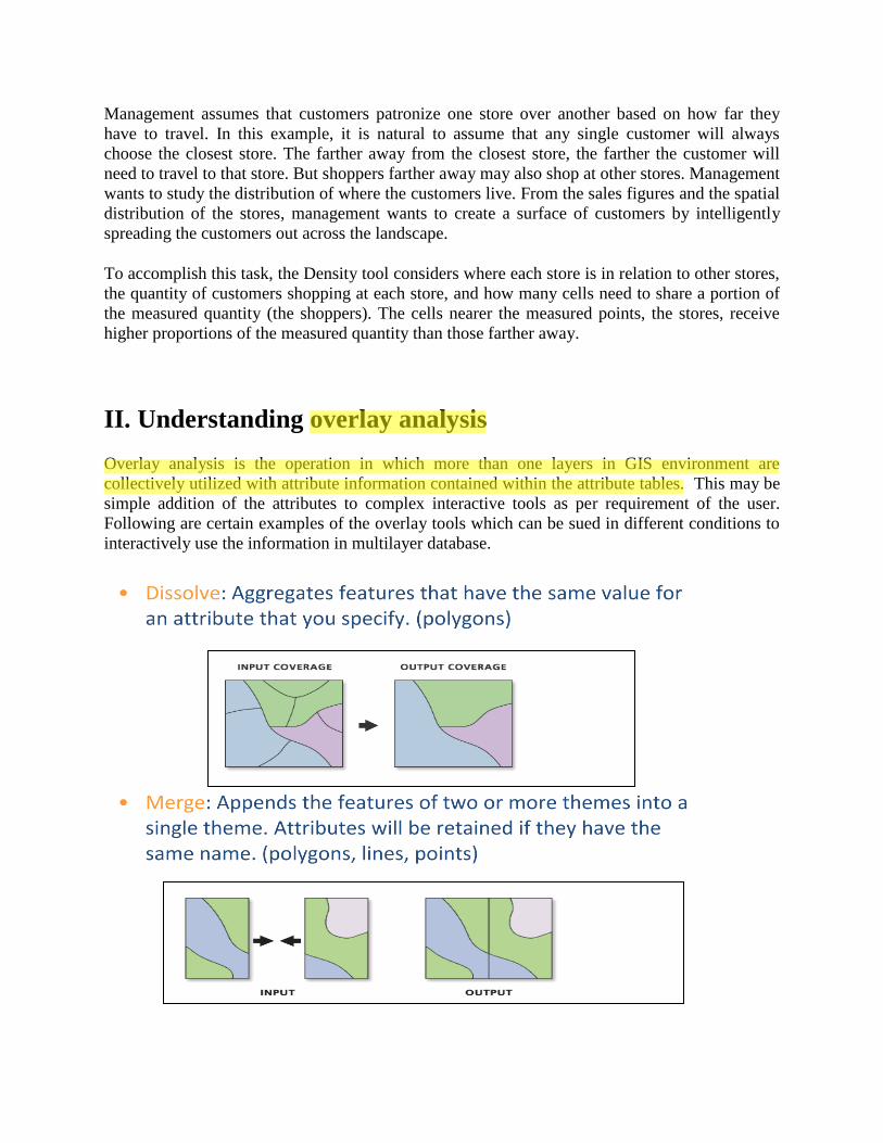
II. Understanding overlay analysis
Overlay analysis is the operation in which more than one layers in GIS environment are
collectively utilized with attribute information contained within the attribute tables. This may be
simple addition of the attributes to complex interactive tools as per requirement of the user.
Following are certain examples of the overlay tools which can be sued in different conditions to
interactively use the information in multilayer database.
hp
Highlight
hp
Highlight
Overlay analysis is a group of methodologies applied in optimal site selection or suitability
modeling. It is a technique for applying a common scale of values to diverse and dissimilar
inputs to create an integrated analysis.
Suitability models identify the best or most preferred locations for a specific phenomenon. Types
of problems addressed by suitability analysis include:
Where to site a new housing development
Which sites are better for deer habitat
Where economic growth is most likely to occur
Where the locations are that are most susceptible to mud slides
Overlay analysis often requires the analysis of many different factors. For instance, choosing the
site for a new housing development means assessing such things as land cost, proximity to
existing services, slope, and flood frequency. This information exists in different rasters with
different value scales: dollars, distances, degrees, and so on. You cannot add a raster of land cost
(dollars) to a raster of distance to utilities (meters) and obtain a meaningful result.
Additionally, the factors in your analysis may not be equally important. It may be that the cost of
land is more important in choosing a site than the distance to utility lines. How much more
important is for you to decide.
Even within a single raster, you must prioritize values. Some values in a particular raster may be
ideal for your purposes (for example, slopes of 0 to 5 degrees), while others may be good, others
bad, and still others unacceptable.
The following lists the general steps to perform overlay analysis:
1. Define the problem.
2. Break the problem into submodels.
3. Determine significant layers.
4. Reclassify or transform the data within a layer.
5. Weight the input layers.
6. Add or combine the layers.
7. Analyze.
Steps 1–3 are common steps for nearly all spatial problem solving and are particularly important
in overlay analysis.
1. Define the problem
Defining the problem is one of the most difficult aspects of the modeling process. The overall
objective must be identified. All aspects of the remaining steps of the overlay modeling process
must contribute to this overall objective.
The components relating to the objective must be defined. Some of the components may be
complimentary, and others competitive. However, a clear definition of each component and how
they interact must be established.
Not only is it important to identify what the problem is, a clear understanding needs to be
developed to define when the problem is solved, or when the phenomenon is satisfied. In the
problem definition, specific measures should be established to identify the success of the
outcome from the model.
For example, when identifying the best location for a ski resort, the overall goal may be to make
money. All factors that are identified in the model should help the ski area be profitable.
2. Break the problem into sub-models
Most overlay problems are complex, and it is recommended that you break them down into
submodels for clarity, to organize your thoughts, and to more effectively solve the overlay
problem.
For example, a suitability model for identifying the best location for a ski resort can be broken
into a series of submodels that all help the ski area be profitable. The first submodel can be a
terrain submodel identifying locations that have a wide variety of favorable terrain for skiers and
snowboarders.
hp
Highlight
hp
Highlight
hp
Highlight
hp
Highlight
hp
Highlight
3. Determine significant layers
The attributes or layers that affect each submodel need to be identified. Each factor captures and
describes a component of the phenomena the submodel is defining. Each factor contributes to the
goals of the submodel, and each submodel contributes to the overall goal of the overlay model.
All and only factors that contribute to defining the phenomenon should be included in the
overlay model.
For certain factors, the layers may need to be created. For example, it may be more desirable to
be closer to a major road. To identify the distance each cell is from a road, Euclidean Distance
may be run to create the distance raster.
Because of the potential different ranges of values and the different types of numbering systems
each input layer may have, before the multiple factors can be combined for analysis, each must
be reclassified or transformed to a common ratio scale.
Common scales can be predetermined, such as a 1 to 9 or a 1 to 10 scale, with the higher value
being more favorable, or the scale can be on a 0 to 1 scale, defining the possibility of belonging
to a specific set.
4. Weight
Certain factors may be more important to the overall goal than others. If this is the case, before
the factors are combined, the factors can be weighted based on their importance. For example, in
the building submodel for siting the ski resort, the slope criteria may be twice as important to the
cost of construction as the distance from a road. Therefore, before combining the two layers, the
slope criteria should be multiplied twice as much as distance to roads.
6. Add/Combine
In overlay analysis, it is desirable to establish the relationship of all the input factors together to
identify the desirable locations that meet the goals of the model. For example, the input layers,
once weighted appropriately, can be added together in an additive weighted overlay model. In
this combination approach, it is assumed that the more favorable the factors, the more desirable
the location will be. Thus, the higher the value on the resulting output raster, the more desirable
the location will be.
Other combining approaches can be applied. For example, in a fuzzy logic overlay analysis, the
combination approaches explore the possibility of membership of a location to multiple sets.
7. Analyze
hp
Highlight
hp
Highlight
hp
Highlight
hp
Highlight
hp
Highlight
hp
Highlight
The final step in the modeling process is for you to analyze the results. Do the potential ideal
locations sensibly meet the criteria? It may be beneficial not only to explore the best locations
identified by the model but to also investigate the second and third most favorable sites.
The identified locations should be visited. You need to validate what you think is there is
actually there. Things could have changed since the data for the model was created. For example,
views may be one of the input criteria to the model; the better the view, the more preferred the
location will be. From the input elevation data, the model identified the locations with the best
views; however, when one of the favorable sites is visited, it is discovered that a building has
been constructed in front of the location, obstructing the view.
Taking the input from all of the steps above, a location is selected.
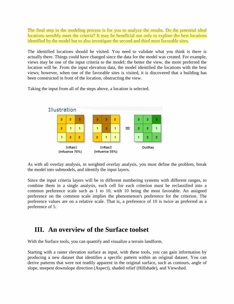
As with all overlay analysis, in weighted overlay analysis, you must define the problem, break
the model into submodels, and identify the input layers.
Since the input criteria layers will be in different numbering systems with different ranges, to
combine them in a single analysis, each cell for each criterion must be reclassified into a
common preference scale such as 1 to 10, with 10 being the most favorable. An assigned
preference on the common scale implies the phenomenon's preference for the criterion. The
preference values are on a relative scale. That is, a preference of 10 is twice as preferred as a
preference of 5.
III. An overview of the Surface toolset
With the Surface tools, you can quantify and visualize a terrain landform.
Starting with a raster elevation surface as input, with these tools, you can gain information by
producing a new dataset that identifies a specific pattern within an original dataset. You can
derive patterns that were not readily apparent in the original surface, such as contours, angle of
slope, steepest downslope direction (Aspect), shaded relief (Hillshade), and Viewshed.
hp
Highlight
hp
Highlight
hp
Highlight
Each surface tool provides insight into a surface that can be used as an end in itself or as input
into additional analysis.
Tool Description
Aspect
Derives aspect from a raster surface. The aspect identifies the downslope
direction of the maximum rate of change in value from each cell to its neighbors.
Contour Creates a line feature class of contours (isolines) from a raster surface.
Contour List Creates a feature class of selected contour values from a raster surface.
Contour with
Barriers
Creates contours from a raster surface. The inclusion of barrier features will
allow one to independently generate contours on either side of a barrier.
Curvature Calculates the curvature of a raster surface, optionally including profile and plan
curvature.
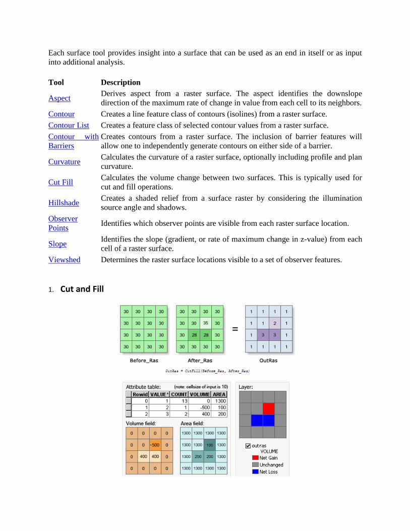
Cut Fill
Calculates the volume change between two surfaces. This is typically used for
cut and fill operations.
Hillshade
Creates a shaded relief from a surface raster by considering the illumination
source angle and shadows.
Observer
Points
Identifies which observer points are visible from each raster surface location.
Slope
Identifies the slope (gradient, or rate of maximum change in z-value) from each
cell of a raster surface.
Viewshed Determines the raster surface locations visible to a set of observer features.
1. Cut and Fill
IV. Types of network analysis layers
Network Analyst allows you to solve common network problems, such as finding the best route
across a city, finding the closest emergency vehicle or facility, identifying a service area around a
location, servicing a set of orders with a fleet of vehicles, or choosing the best facilities to open
or close.
• Network: a set of interconnected line entities, whose attributes share some common
theme primarily related to flow
• Network in GIS: a topology-based line coverage
• Geometric Network in ArcGIS: a feature data set comprised of feature classes: edges and
junctions, and their connectivity defined by topology rules
Network Elements
• Links - “Conduits” for movement
• Intersections - Link joins
• Stops - Sources/sinks where resources can enter or exit the network
• Centers - node locations which may receive or provide
resources. Attributes for total amount of resource supplied to
or taken from a center, e.g., total water capacity for a reservoir
• Barriers - nodes which prevent flow through links, or links with infinite impedance
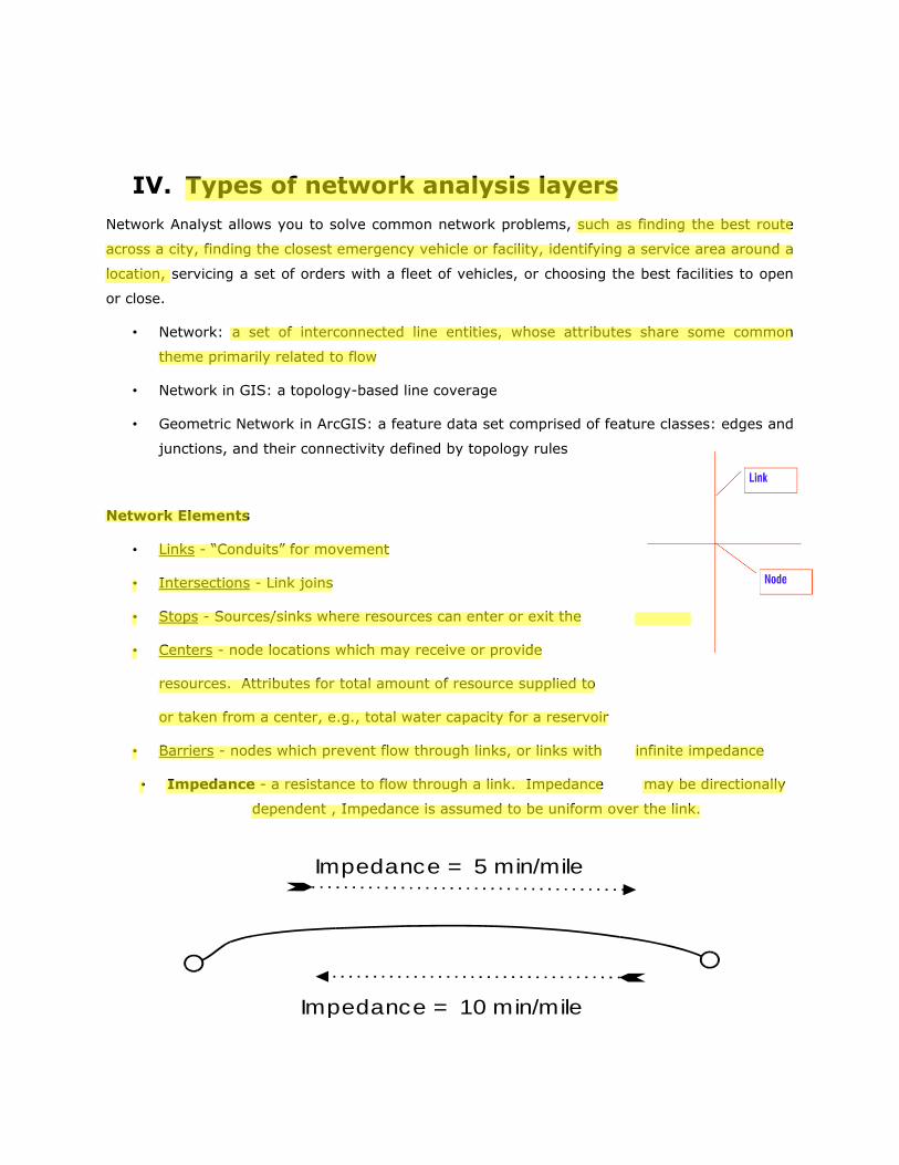
• Impedance - a resistance to flow through a link. Impedance may be directionally
dependent , Impedance is assumed to be uniform over the link.
Impedance = 5 min/mile
Impedance = 10 min/mile
hp
Highlight
hp
Highlight
hp
Highlight
hp
Highlight
hp
Highlight

Preparing a Network
Step 1: Prepare a network coverage,
Step 2: edit the coverage to represent network elements and update its topology
Step 3: attribute with link impedances
Step 4: generate attribute based on input attributes
Step 5: display results
Network Applications
1. Shortest / Critical Path Analysis
Paths, flow, tours
2. Allocation
Supply, impedance
3. Location-Allocation
supply and demand, objective function
Shortest Path Analysis
Finding the shortest or least-cost manner in which to visit a series of locations in a
network. The cost may be determined by distance or by travel-time or a
combination of factors calculated as a cost value.
Often the parameter that is minimized in path finding is travel time. This factors in
things like topography, traffic volume, average speed, stops etc.
The Dijkstra’s algorithm is used to solve a single-source shortest-path problem
hp
Highlight
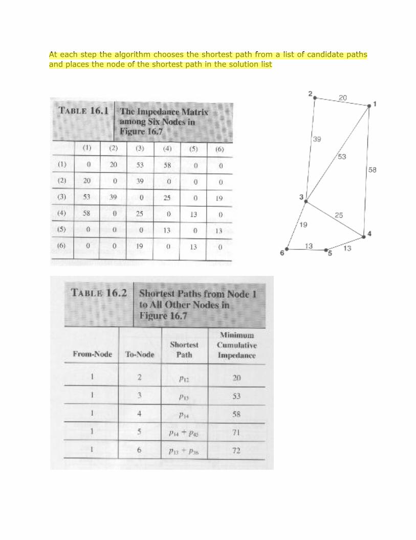
At each step the algorithm chooses the shortest path from a list of candidate paths
and places the node of the shortest path in the solution list
hp
Highlight

Route
Network Analyst can find the best way to get from one location to another or to visit several
locations. The locations can be specified interactively by placing points on the screen, entering an
address, or using points in an existing feature class or feature layer. If you have more than two
stops to visit, the best route can be determined for the order of locations as specified by the
user. Alternatively, ArcGIS Network Analyst can determine the best sequence to visit the
locations.
What's the best route?
Whether finding a simple route between two locations or one that visits several locations, people
usually try to take the best route. But "best route" can mean different things in different
situations.
The best route can be the quickest, shortest, or most scenic route, depending on the impedance
chosen. If the impedance is time, then the best route is the quickest route. Hence, the best route
can be defined as the route that has the lowest impedance, where the impedance is chosen by
the user. Any valid network cost attribute can be used as the impedance when determining the
best route.
In the example below, the first case uses time as an impedance. The quickest path is shown in
blue and has a total length of 4.5 miles, which takes 8 minutes to traverse.
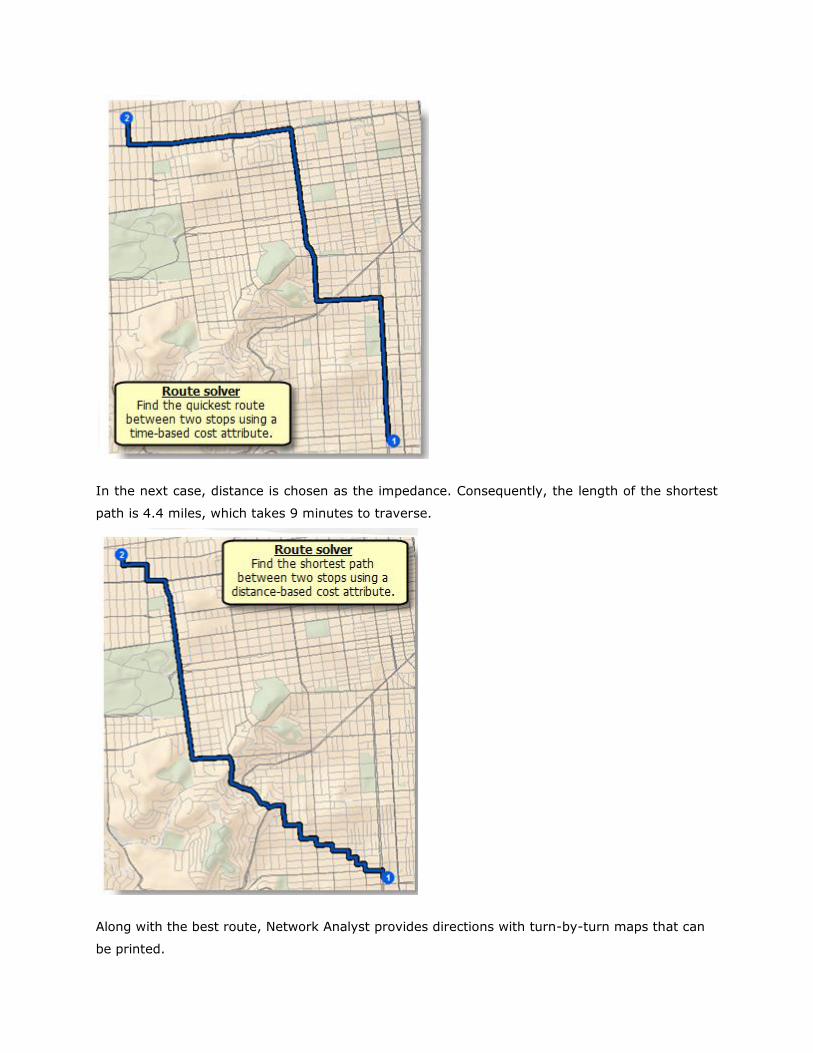
In the next case, distance is chosen as the impedance. Consequently, the length of the shortest
path is 4.4 miles, which takes 9 minutes to traverse.
Along with the best route, Network Analyst provides directions with turn-by-turn maps that can
be printed.
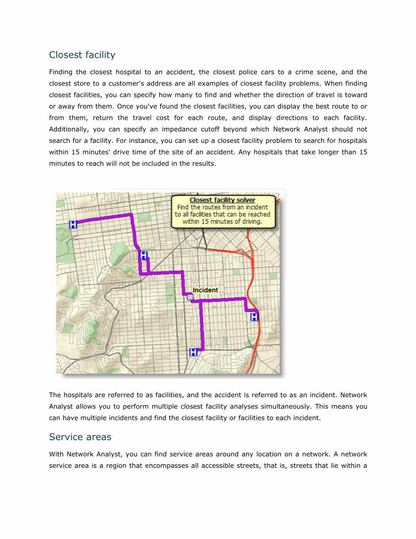
Closest facility
Finding the closest hospital to an accident, the closest police cars to a crime scene, and the
closest store to a customer's address are all examples of closest facility problems. When finding
closest facilities, you can specify how many to find and whether the direction of travel is toward
or away from them. Once you've found the closest facilities, you can display the best route to or
from them, return the travel cost for each route, and display directions to each facility.
Additionally, you can specify an impedance cutoff beyond which Network Analyst should not
search for a facility. For instance, you can set up a closest facility problem to search for hospitals
within 15 minutes' drive time of the site of an accident. Any hospitals that take longer than 15
minutes to reach will not be included in the results.
The hospitals are referred to as facilities, and the accident is referred to as an incident. Network
Analyst allows you to perform multiple closest facility analyses simultaneously. This means you
can have multiple incidents and find the closest facility or facilities to each incident.
Service areas
With Network Analyst, you can find service areas around any location on a network. A network
service area is a region that encompasses all accessible streets, that is, streets that lie within a
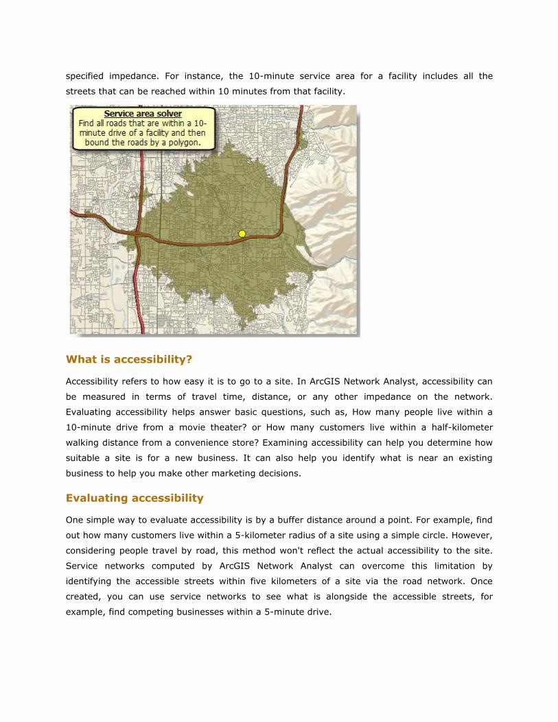
specified impedance. For instance, the 10-minute service area for a facility includes all the
streets that can be reached within 10 minutes from that facility.
What is accessibility?
Accessibility refers to how easy it is to go to a site. In ArcGIS Network Analyst, accessibility can
be measured in terms of travel time, distance, or any other impedance on the network.
Evaluating accessibility helps answer basic questions, such as, How many people live within a
10-minute drive from a movie theater? or How many customers live within a half-kilometer
walking distance from a convenience store? Examining accessibility can help you determine how
suitable a site is for a new business. It can also help you identify what is near an existing
business to help you make other marketing decisions.
Evaluating accessibility
One simple way to evaluate accessibility is by a buffer distance around a point. For example, find
out how many customers live within a 5-kilometer radius of a site using a simple circle. However,
considering people travel by road, this method won't reflect the actual accessibility to the site.
Service networks computed by ArcGIS Network Analyst can overcome this limitation by
identifying the accessible streets within five kilometers of a site via the road network. Once
created, you can use service networks to see what is alongside the accessible streets, for
example, find competing businesses within a 5-minute drive.
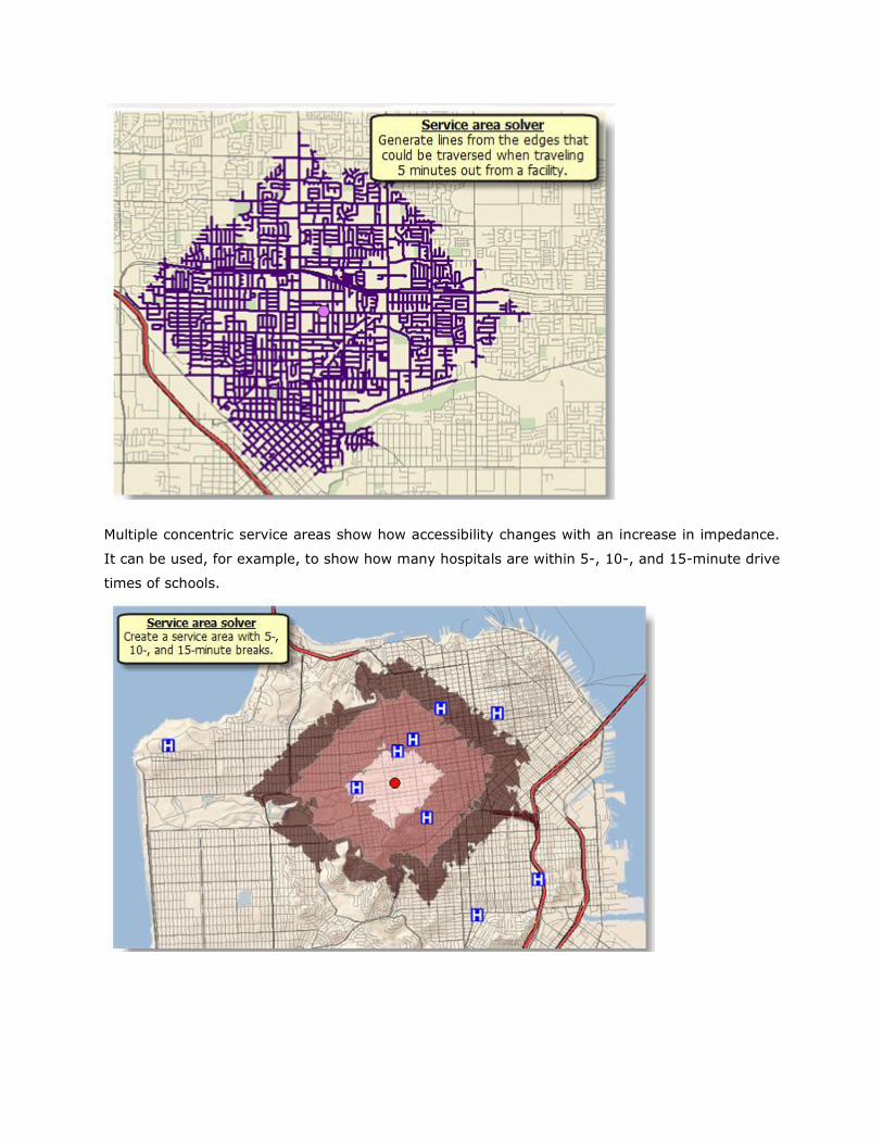
Multiple concentric service areas show how accessibility changes with an increase in impedance.
It can be used, for example, to show how many hospitals are within 5-, 10-, and 15-minute drive
times of schools.
V. Location-allocation
Location-allocation helps you choose which facilities from a set of facilities to operate based on
their potential interaction with demand points. It can help you answer questions like the
following:
Given a set of existing fire stations, which site for a new fire station would provide the
best response times for the community?
If a retail company has to downsize, which stores should it close to maintain the most
overall demand?
Where should a factory be built to minimize the distance to distribution centers?
In these examples, facilities would represent the fire stations, retail stores, and factories;
demand points would represent buildings, customers, and distribution centers.
The objective may be to minimize the overall distance between demand points and facilities,
maximize the number of demand points covered within a certain distance of facilities, maximize
an apportioned amount of demand that decays with increasing distance from a facility, or
maximize the amount of demand captured in an environment of friendly and competing facilities.
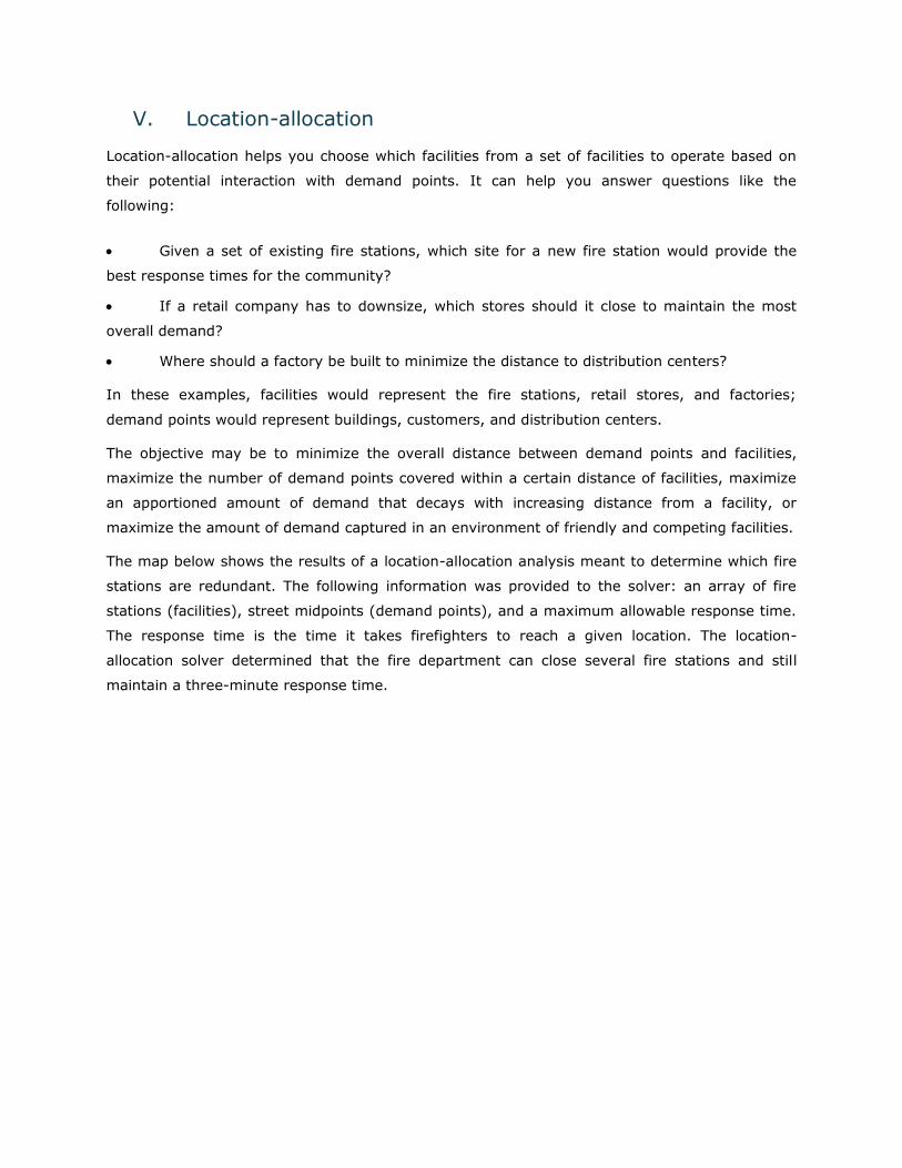
The map below shows the results of a location-allocation analysis meant to determine which fire
stations are redundant. The following information was provided to the solver: an array of fire
stations (facilities), street midpoints (demand points), and a maximum allowable response time.
The response time is the time it takes firefighters to reach a given location. The location-
allocation solver determined that the fire department can close several fire stations and still
maintain a three-minute response time.
VI. Buffer (Analysis)
One of the most basic questions asked of a GIS is "what's near what?" For example:
How close is this well to a landfill?
Do any roads pass within 1,000 meters of a stream?
What is the distance between two locations?
What is the nearest or farthest feature from something?
What is the distance between each feature in a layer and the features in another layer?
What is the shortest street network route from some location to another?
The Proximity toolset contains tools that are used to determine the proximity of features
within one or more feature classes or between two feature classes. These tools can identify
features that are closest to one another or calculate the distances between or around them.
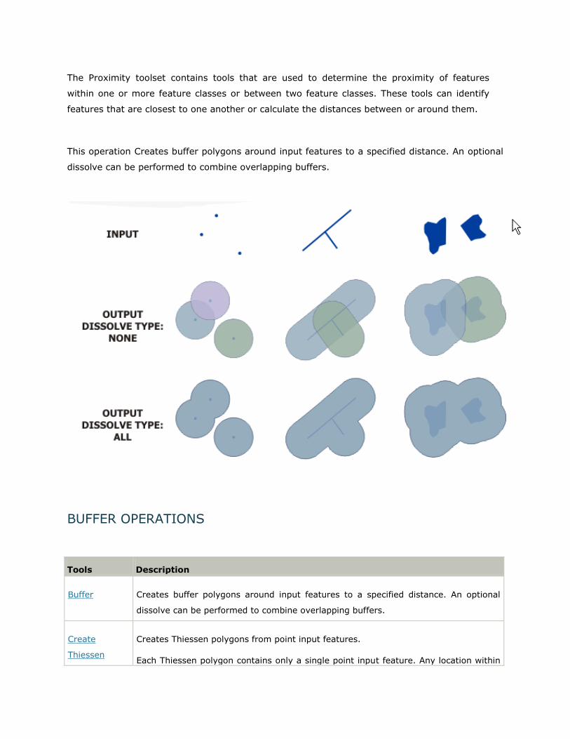
This operation Creates buffer polygons around input features to a specified distance. An optional
dissolve can be performed to combine overlapping buffers.
BUFFER OPERATIONS
Tools Description
Buffer Creates buffer polygons around input features to a specified distance. An optional
dissolve can be performed to combine overlapping buffers.
Create
Thiessen
Creates Thiessen polygons from point input features.
Each Thiessen polygon contains only a single point input feature. Any location within
Polygons a Thiessen polygon is closer to its associated point than to any other point input
feature.
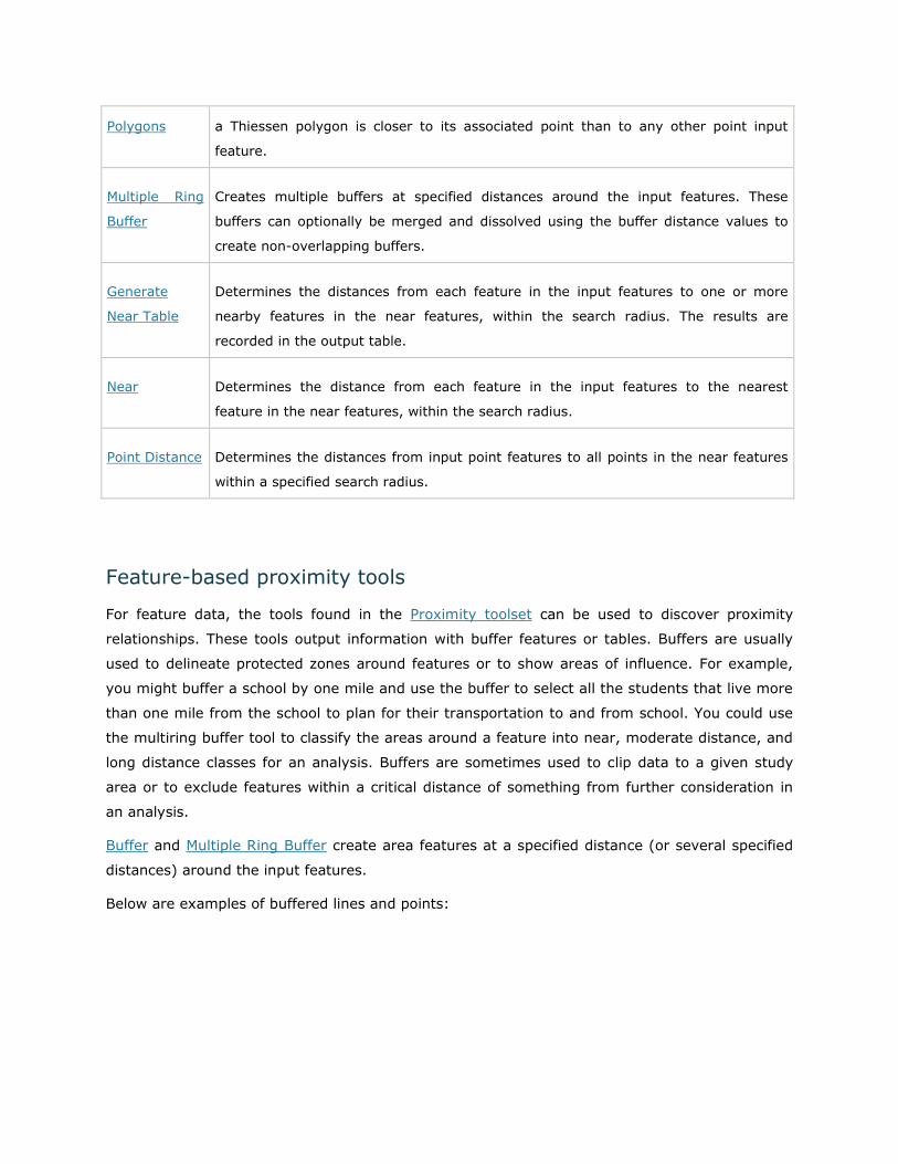
Multiple Ring
Buffer
Creates multiple buffers at specified distances around the input features. These
buffers can optionally be merged and dissolved using the buffer distance values to
create non-overlapping buffers.
Generate
Near Table
Determines the distances from each feature in the input features to one or more
nearby features in the near features, within the search radius. The results are
recorded in the output table.
Near Determines the distance from each feature in the input features to the nearest
feature in the near features, within the search radius.
Point Distance Determines the distances from input point features to all points in the near features
within a specified search radius.
Feature-based proximity tools
For feature data, the tools found in the Proximity toolset can be used to discover proximity
relationships. These tools output information with buffer features or tables. Buffers are usually
used to delineate protected zones around features or to show areas of influence. For example,
you might buffer a school by one mile and use the buffer to select all the students that live more
than one mile from the school to plan for their transportation to and from school. You could use
the multiring buffer tool to classify the areas around a feature into near, moderate distance, and
long distance classes for an analysis. Buffers are sometimes used to clip data to a given study
area or to exclude features within a critical distance of something from further consideration in
an analysis.
Buffer and Multiple Ring Buffer create area features at a specified distance (or several specified
distances) around the input features.
Below are examples of buffered lines and points:
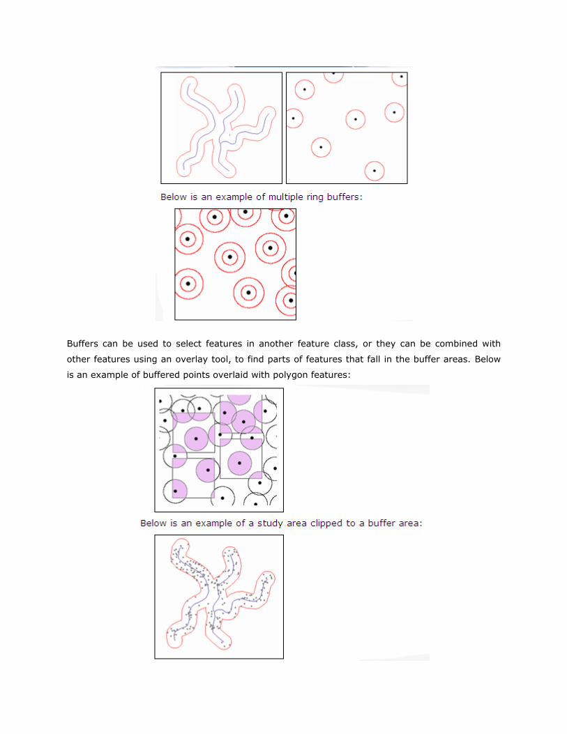
Buffers can be used to select features in another feature class, or they can be combined with
other features using an overlay tool, to find parts of features that fall in the buffer areas. Below
is an example of buffered points overlaid with polygon features:
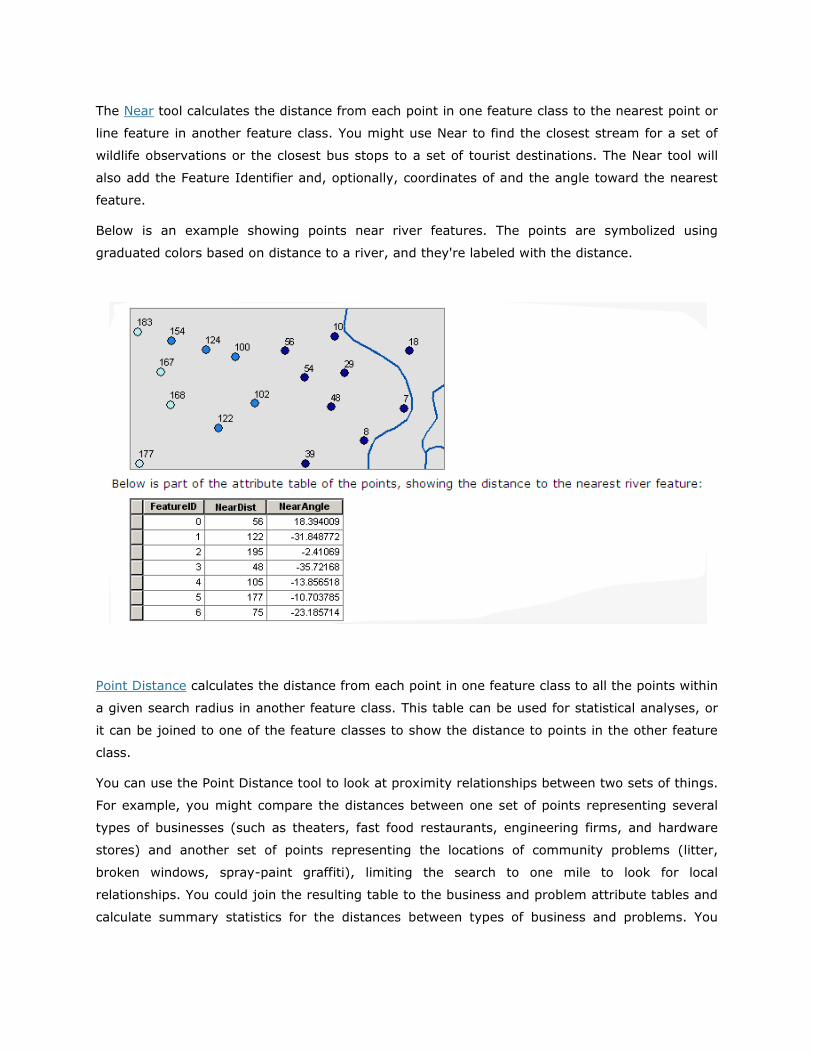
The Near tool calculates the distance from each point in one feature class to the nearest point or
line feature in another feature class. You might use Near to find the closest stream for a set of
wildlife observations or the closest bus stops to a set of tourist destinations. The Near tool will
also add the Feature Identifier and, optionally, coordinates of and the angle toward the nearest
feature.
Below is an example showing points near river features. The points are symbolized using
graduated colors based on distance to a river, and they're labeled with the distance.
Point Distance calculates the distance from each point in one feature class to all the points within
a given search radius in another feature class. This table can be used for statistical analyses, or
it can be joined to one of the feature classes to show the distance to points in the other feature
class.
You can use the Point Distance tool to look at proximity relationships between two sets of things.
For example, you might compare the distances between one set of points representing several
types of businesses (such as theaters, fast food restaurants, engineering firms, and hardware
stores) and another set of points representing the locations of community problems (litter,
broken windows, spray-paint graffiti), limiting the search to one mile to look for local
relationships. You could join the resulting table to the business and problem attribute tables and
calculate summary statistics for the distances between types of business and problems. You

might find a stronger correlation for some pairs than for others and use your results to target the
placement of public trash cans or police patrols.
You might also use Point Distance to find the distance and direction to all the water wells within a
given distance of a test well where you identified a contaminant.
Below is an example of point distance analysis. Each point in one feature class is given the ID,
distance, and direction to the nearest point in another feature class.
Below is the Point Distance table, joined to one set of points and used to select the points
that are closest to point 55.
Both Near and Point Distance return the distance information as numeric attributes in the input
point feature attribute table for Near and in a stand-alone table that contains the Feature IDs of
the Input and Near features for Point Distance.
Create Thiessen Polygons creates polygon features that divide the available space and allocate it
to the nearest point feature. The result is similar to the Euclidean Allocation tool for rasters.
Thiessen polygons are sometimes used instead of interpolation to generalize a set of sample
measurements to the areas closest to them. Thiessen polygons are sometimes also known as
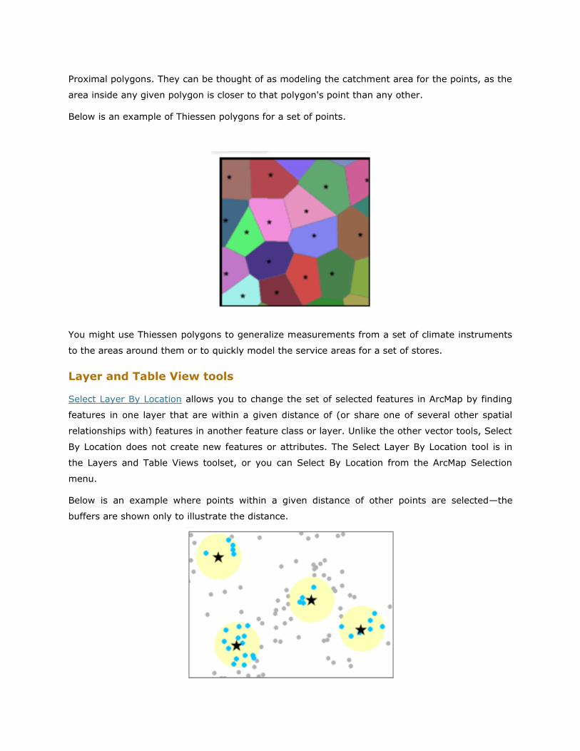
Proximal polygons. They can be thought of as modeling the catchment area for the points, as the
area inside any given polygon is closer to that polygon's point than any other.
Below is an example of Thiessen polygons for a set of points.
You might use Thiessen polygons to generalize measurements from a set of climate instruments
to the areas around them or to quickly model the service areas for a set of stores.
Layer and Table View tools
Select Layer By Location allows you to change the set of selected features in ArcMap by finding
features in one layer that are within a given distance of (or share one of several other spatial
relationships with) features in another feature class or layer. Unlike the other vector tools, Select
By Location does not create new features or attributes. The Select Layer By Location tool is in
the Layers and Table Views toolset, or you can Select By Location from the ArcMap Selection
menu.
Below is an example where points within a given distance of other points are selected—the
buffers are shown only to illustrate the distance.
Network distance tools
Some distance analyses require that the measurements be constrained to a road, stream, or
other linear network. Network Analyst lets you find the shortest route to a location along a
network of transportation routes, find the closest point to a given point, or build service areas
(areas that are equally distant from a point along all available paths) in a transportation network.
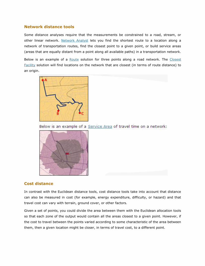
Below is an example of a Route solution for three points along a road network. The Closest
Facility solution will find locations on the network that are closest (in terms of route distance) to
an origin.
Cost distance
In contrast with the Euclidean distance tools, cost distance tools take into account that distance
can also be measured in cost (for example, energy expenditure, difficulty, or hazard) and that
travel cost can vary with terrain, ground cover, or other factors.
Given a set of points, you could divide the area between them with the Euclidean allocation tools
so that each zone of the output would contain all the areas closest to a given point. However, if
the cost to travel between the points varied according to some characteristic of the area between
them, then a given location might be closer, in terms of travel cost, to a different point.

Below is an example of using the Cost Allocation tool, where travel cost increases with land-
cover type. The dark areas could represent difficult-to-traverse swamps, and the light areas
could represent more easily traversed grassland.
This is in some respects a more complicated way of dealing with distance than using straight
lines, but it is very useful for modeling movement across a surface that is not uniform.
Below is an example that contrasts the surface length of a line feature in rough terrain with its
planimetric length.
Proximity tools
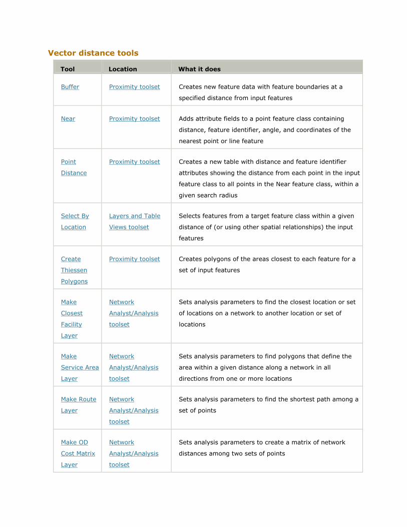
Vector distance tools
Tool Location What it does
Buffer Proximity toolset Creates new feature data with feature boundaries at a
specified distance from input features
Near Proximity toolset Adds attribute fields to a point feature class containing
distance, feature identifier, angle, and coordinates of the
nearest point or line feature
Point
Distance
Proximity toolset Creates a new table with distance and feature identifier
attributes showing the distance from each point in the input
feature class to all points in the Near feature class, within a
given search radius
Select By
Location
Layers and Table
Views toolset
Selects features from a target feature class within a given
distance of (or using other spatial relationships) the input
features
Create
Thiessen
Polygons
Proximity toolset Creates polygons of the areas closest to each feature for a
set of input features
Make
Closest
Facility
Layer
Network
Analyst/Analysis
toolset
Sets analysis parameters to find the closest location or set
of locations on a network to another location or set of
locations
Make
Service Area
Layer
Network
Analyst/Analysis
toolset
Sets analysis parameters to find polygons that define the
area within a given distance along a network in all
directions from one or more locations
Make Route
Layer
Network
Analyst/Analysis
toolset
Sets analysis parameters to find the shortest path among a
set of points
Make OD
Cost Matrix
Layer
Network
Analyst/Analysis
toolset
Sets analysis parameters to create a matrix of network
distances among two sets of points
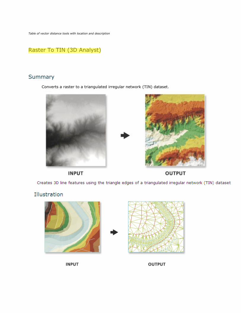
Table of vector distance tools with location and description
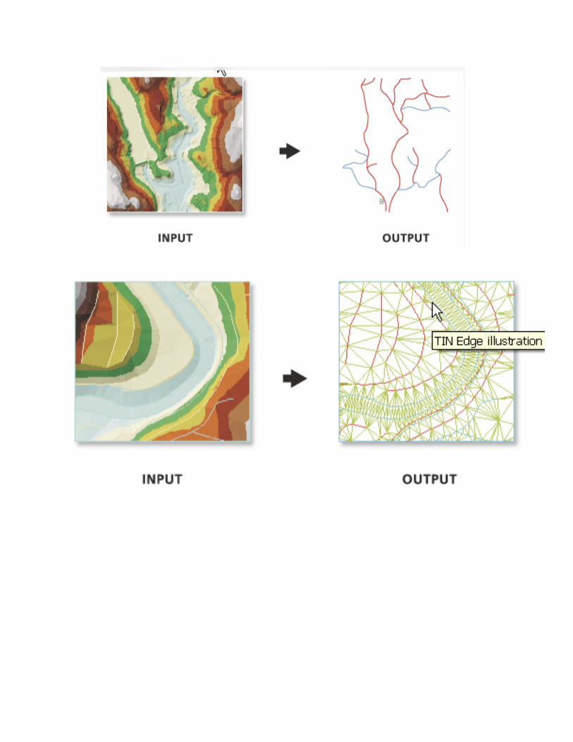
Raster To TIN (3D Analyst)
Summary
Converts a raster to a triangulated irregular network (TIN) dataset.
hp
Highlight
Related Documents