GIS-BASED METHOD TO ASSESS SEISMIC ...

EUR 24275 EN - 2010

GIS-BASED METHOD TO ASSESS SEISMICVULNERABILITY OF INTERCONNECTED

INFRASTRUCTUREA case of EU gas and electricity networks

K. Poljanšek, F. Bono, E. Gutiérrez

The mission of the JRC-IPSC is to provide research results and to support EU policy-makers in their effort towards global security and towards protection of European citizens from accidents, deliberate attacks, fraud and illegal actions against EU policies. European Commission Joint Research Centre Institute for the Protection and Security of the Citizen Contact information Address: Via E. Fermi 2749, TP 480, I-21027 Ispra (VA), Italy E-mail: [email protected] Tel.: +39- 0332-785711 Fax: +39-0332-789049 http://ipsc.jrc.ec.europa.eu/ http://www.jrc.ec.europa.eu/ Legal Notice Neither the European Commission nor any person acting on behalf of the Commission is responsible for the use which might be made of this publication.

Europe Direct is a service to help you find answers to your questions about the European Union Freephone number (*): 00 800 6 7 8 9 10 11 (*) Certain mobile telephone operators do not allow access to 00 800 numbers or these calls may be billed.

A great deal of additional information on the European Union is available on the Internet. It can be accessed through the Europa server http://europa.eu/ JRC 57064 EUR 24275 EN ISBN 978-92-79-15209-2 ISSN 1018-5593 DOI 10.2788/71352

Luxembourg: Publications Office of the European Union

© European Union, 2010 Reproduction is authorised provided the source is acknowledged Printed in Italy

i

Table of Contents

1 PREAMBLE ............................................................................................................................... 1

2 INTRODUCTION ...................................................................................................................... 3

2.1 RESEARCH GOAL AND OBJECTIVES ......................................................................................... 6

2.2 THE OUTLINE OF THE REPORT ................................................................................................. 7

3 ASSEMBLY OF GIS INFORMATION .................................................................................. 8

3.1 GIS PROCESSING .................................................................................................................... 8

3.2 EUROPEAN INTERCONNECTED ENERGY NETWORK ............................................................... 11

3.2.1 Networks interconnections ........................................................................................... 14

3.2.2 Substations' Transmission/Distribution definition ....................................................... 18

3.2.3 Population served by substations ................................................................................. 20

3.2.4 Hazards level................................................................................................................ 23

4 TOPOLOGY OF NETWORK DATASETS.......................................................................... 25

4.1 SOURCES AND SINKS ............................................................................................................. 28

5 HAZARD AND RISK ASSESSMENT .................................................................................. 31

5.1 SEISMIC HAZARD AND RISK .................................................................................................. 32

5.1.1 Seismic hazard maps .................................................................................................... 33

5.1.2 Fragility curves ............................................................................................................ 36

5.1.2.1 Electricity power system....................................................................................... 37

5.1.2.2 Natural gas system ................................................................................................ 41

6 PROBABILISTIC RELIABILITY MODEL ........................................................................ 45

6.1 PERFORMANCE MEASURES ................................................................................................... 46

6.1.1 Connectivity loss .......................................................................................................... 46

6.1.2 Power loss .................................................................................................................... 48

ii

6.1.3 Impact factor on the population ................................................................................... 48

6.2 SEISMIC PERFORMANCE NETWORK ANALYSIS ....................................................................... 49

6.2.1 Applied terms ............................................................................................................... 49

6.2.2 Monte Carlo simulations .............................................................................................. 51

6.2.3 Algorithm ..................................................................................................................... 52

7 PROBABILISTIC MODEL FOR NETWORK INTERDEPENDENCY........................... 54

7.1 FUNDAMENTAL INTERDEPENDENCE...................................................................................... 54

7.2 INTEROPERABILITY MATRIX ................................................................................................. 56

7.3 STRENGTH OF COUPLING APPLICATION ................................................................................. 57

8 RESULTS OF SIMULATIONS ............................................................................................. 62

8.1 INDEPENDENT NETWORK VULNERABILITY ............................................................................ 66

8.2 GAS-SOURCE SUPPLY STREAM FRAGILITY CURVES ............................................................... 71

8.3 DEPENDANT NETWORK VULNERABILITY .............................................................................. 73

8.3.1 Beetweenness centrality attack vs. seismic hazard and strength of coupling .............. 84

8.4 GEOGRAPHICAL SPREAD OF DAMAGE ................................................................................... 88

9 CONCLUSIONS ...................................................................................................................... 93

10 BIBLIOGRAPHY .................................................................................................................... 95

iii

List of Figures

Figure 1: GIS-based method to assess fragility curves for interconnected systems. ........................... 8

Figure 2: European gas pipeline network. Transmission pipelines overlaid with the distribution

network. Link thickness is proportional to the pipeline diameter. ............................................. 11

Figure 3: European electricity network. Transmission lines (in blue) overlaid with the distribution

network (in red). Line thickness is proportional to the voltage. ................................................ 12

Figure 4: Network structure field structure definition in the database table; we show schematically

how the GIS data of a gas network is parsed to generate a connectivity list that can be

converted into a graph structure. Starting from (1) where each individual line segment is

uniquely assigned an identification number (line ID) and its diameter, we then have in (2) the

geographical coordinates of the two end points (vertices) of each line. In (3) the end points are

assigned an ID number consistent with the end points of the line segment. In (4) the data are

condensed into the final tabular structure that can be used to generate a graph. ....................... 13

Figure 5: The Energy Interconnected Network. ................................................................................. 15

Figure 6: Plants and grids connections. ............................................................................................. 16

Figure 7: Breadth first search of the shortest paths between a power station and the substations on

the main network. ....................................................................................................................... 17

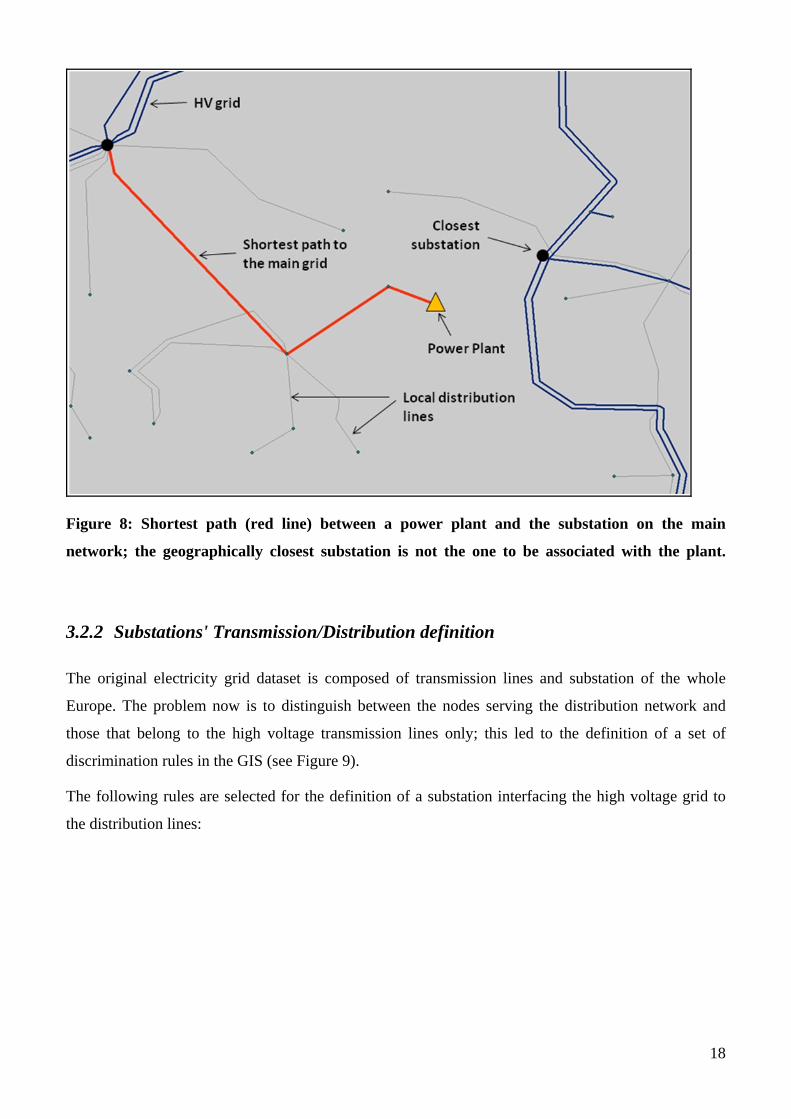
Figure 8: Shortest path (red line) between a power plant and the substation on the main network; the

geographically closest substation is not the one to be associated with the plant. ...................... 18

Figure 9: Distributions substation definition criteria (red points fulfil the single criteria, purple lines

belongs to the minor electricity grid). ........................................................................................ 19

Figure 10: Transmission and Distribution Nodes based on defined criteria. ..................................... 20

Figure 11: Landscan European population density map. ................................................................... 21

Figure 12: GIS processing for the substations' served population definition. ................................... 22

Figure 13: Distribution substation (red dots), population and served areas (greenish polygons) in

France. ........................................................................................................................................ 22

Figure 14: Seismic hazard Map of Europe and electricity substations scaled according to the PGA

value - 10% Probability of exceedance in 50 Years, 475-Year Return Period. ......................... 23

iv

Figure 15: Interconnected system of the gas network (bellow) and electricity network (above) with

gas power plants as the common vertices (in the middle). ........................................................ 25

Figure 16: Vertex degree frequency distributions and their complementary cumulative distribution

of the interconnected system, (a), and its networks,(b) and (c), regarded as undirected

networks. .................................................................................................................................... 27

Figure 17: European map for population density covered with Thiessen polygons. ......................... 29

Figure 18: Seismic risk. ..................................................................................................................... 33

Figure 19: Relation between the return period, exposure time and the probability of exceedence of

the event of given magnitude. .................................................................................................... 34

Figure 20: Example of seismic hazard maps for different hazard levels for Slovenia. ..................... 36

Figure 21: Example of hazard curve for Ljubljana, the capital of Slovenia. ..................................... 36

Figure 22: Fragility curves for low voltage substations with (a) anchored subcomponents and (b)

unanchored subcomponents. ...................................................................................................... 38

Figure 23: Fragility curves for medium voltage substations with (a) anchored subcomponents and

(b) unanchored subcomponents. ................................................................................................ 39

Figure 24: Fragility curves for high voltage substations with (a) anchored subcomponents and (b)


Figure 25: Fragility curves for small power plants with (a) anchored subcomponents and (b)


Figure 26: Fragility curves for medium/large power plants with (a) anchored subcomponents and

(b) unanchored subcomponents. ................................................................................................ 41

Figure 27: Fragility curves for compressor stations with (a) anchored subcomponents and (b)


Figure 28: Repair rate for the pipelines (a) and fragility curves (b) for the different length of the

pipeline. ...................................................................................................................................... 44

Figure 29: Propagation of probabilities of elements failure through the analysis. ............................ 45

Figure 30: Monte Carlo simulations scheme. .................................................................................... 51

Figure 31: The algorithm applied in the MatLab procedure. ............................................................. 53

v

Figure 32: Venn diagram: (a) failure of the electricity vertex and (b) conditional probability of

failure of electricity vertex because of dependency on the gas network due to the failure of the

gas vertex. .................................................................................................................................. 58

Figure 33: Strength of coupling in Venn’s diagrams. ........................................................................ 59

Figure 34: Schema of gas-source supply stream of the gas power plant. .......................................... 60

Figure 35: Seismic hazard map of peak ground acceleration for 475 year return period and 10%

probability of exceedence in the 50 years of exposure time (Giardini et al., 2003). ................. 63

Figure 36: European gas network: The relative sizes of the vertices correspond to the PGA of their

location obtained from the 475 return period seismic hazard map. ........................................... 64

Figure 37: European electricity network: The relative sizes of the vertices correspond to the PGA of

their location obtained from the 475 return period seismic hazard map. ................................... 65

Figure 38: Results of Monte Carlo simulations in the case of European gas network presented for

different hazard levels as complementary cumulative distribution function (a) and summarized

in network fragility curves for different damage states (b). ....................................................... 67

Figure 39: Results of Monte Carlo simulations in the case of European electricity network presented

for different hazard levels as complementary cumulative distribution function (a) and

summarized in network fragility curves for different damage states (b). .................................. 67

Figure 40: Results of Monte Carlo simulations in the case of electricity network of Italy presented


summarized in network fragility curves for different damage states (b). .................................. 68

Figure 41: European gas network: the size of the vertices and the width of the lines correspond to

the probability of failure according to 475 return period seismic hazard map. ......................... 69

Figure 42: European electricity network: the sizes of the vertices correspond to the probability of

failure according to 475 return period seismic hazard map. ...................................................... 70

Figure 43: The gas-source supply stream fragility curves for all gas power plants. .......................... 71

Figure 44: European electricity network: the probability of failure of gas vertices adjacent to gas

power plants in the case of hazard level of 475 return period seismic hazard map. .................. 72

Figure 45: Share of gas power plants out of all power plants measured in electricity power

generation capacity (green) and in number of facilities (blue) in percentage by the country. ... 75

vi

Figure 46: Electricity power generation from gas power plants and the other power plants presented

as an absolute value in MW and as a share of electricity power generation covered by gas

power plants in percentage by the country................................................................................. 76

Figure 47: Frequency distribution of the nominal power of the power plants and the population

assigned to the distribution substations in the European electricity network. ........................... 77

Figure 48: Dependent network fragility curves for EU electricity network at different damage states

in terms of Connectivity loss as performance measure. ............................................................. 78

Figure 49: Dependent network fragility curves for EU electricity network and different damage

states in terms of power loss as performance measure. ............................................................. 79


states in terms of impact factor on the population as performance measure. ............................ 80

Figure 51: Dependent network fragility curves for IT electricity network and different damage

states in terms of connectivity loss as performance measure..................................................... 81


states in terms of power loss as performance measure. ............................................................. 82


states in terms of impact factor on the population as performance measure. ............................ 83

Figure 54: Vertex betweenness centrality in EU electricity network. ............................................... 85

Figure 55: Comparison between the betweenness centrality attack and seismic hazard with different

strength of coupling for the case of EU electricity grid. ............................................................ 87

Figure 56: Comparison between the betweenness centrality attack and seismic hazard with different

strength of coupling for the case of IT electricity grid. ............................................................. 87

Figure 57: Geographical spread of power loss for 100% of strength of coupling and PGA factor

from 0.8 – 2.5. ............................................................................................................................ 90

Figure 58: Comparison between the strength of coupling 0 and 100% at PGA factor 1. .................. 90

Figure 59: Comparison between the strength of coupling 0 and 100% at PGA factor 2.5. ............... 91

Figure 60: Affected population for the strength of coupling 100% and PGA factor 2.5. .................. 92

vii

List of Tables

Table 1 - GIS datasets sources ............................................................................................................. 9

Table 2: Topological characteristics of the interconnected system and its component networks. .... 26

Table 3: Division of vertices according to their functionality. .......................................................... 28

Table 4: Correlations between different ground motion parameters for description of an earthquake

event. .......................................................................................................................................... 43

Table 5: Maximum expected PGA in networks while applying different general PGA factor. ........ 62

Table 6: Average probabilities of failure of gas power plants due to earthquake and of gas vertices

adjacent to gas power plants. ..................................................................................................... 73

1

1 Preamble

The issue of vulnerability of critical infrastructures has recently attracted considerable attention

from both the academic and policy-making spheres. It is not surprising that, in view of the complex

behaviour of modern-day infrastructure systems, many researchers suggested that the study of the

connections that make up such infrastructures could be effectively represented in terms of graphs. It

would appear to be noteworthy that the findings in a purely mathematical subject matter

(combinatorics and graph theory) could have an application in the realm of politics and social

policy in —what appears to be— such a short period; however, it is not the first time such an

approach was taken, because modern graph theory has its origins in the Seven Bridges of

Köningberg problem solved by Euler nearly three-hundred years ago.

The mathematical field of graph theory has, for the major part of the intervening period since its

inception, been the subject of much theoretical dissertation; however, over the last decade it has

been adopted by the research community as one of the main mathematical methods in the armoury

of, so-called, complex systems analysis.

It was soon realised that although graph theory had developed a broad range of interesting results

for certain classes of graphs, real-world networks were characterised by interconnection topologies

that had, hitherto, not been studied or considered. Important steps were taken by extending the

concepts of the topology of random graphs proposed by Erdös-Renyi to, so-called, Small-World

(Watts and Strogatz [25]) and Scale-Free graphs (Barabási and Albert [3]).

In particular, in view of the similarities between these pseudo-random graphs and the graphs of real-

world systems, considerable attention was paid to understanding how these reacted to certain kinds

of ‘attacks’. By ‘attack’ we mean the generic elimination of part of the real-networks’ constituent

elements (which for its corresponding graph are represented by its nodes and connecting edges),

which could be either the result of an intentional plan, a random process or, as is done here, due to

the actions of some natural process (earthquake, storm, ageing, etc).

Research on the nature of attack vulnerability was successfully conducted on many types or real-

world networks; however, it was obvious that this was not the whole picture. Real-world networks

are interconnected to other critical infrastructures, either by physical, operational or social ties. So,

in reality, critical infrastructures are not many but actually only one: that mega-infrastructure that

encompasses all our daily activities. Clearly, developing an analysis for this all-enveloping mega-

2

infrastructure is not feasible, but we can take some steps into understanding how, at least, two types

of infrastructure depend on each other, and how their interdependence affects their aggregate

vulnerability. More specifically, what we address in this document is how a natural hazard (here an

earthquake) not only explicitly generates vulnerabilities in a given network (here the European

Electricity transmission grid), but how the vulnerability of another network on which it is partially

dependent (here the European Gas Transmission network) induces a second, implicit, vulnerability

by virtue of their interconnections.

We study two important issues of modern interdependent critical infrastructure systems: first we

assess the network response under seismic hazard; then we analyse the increased vulnerability due

to coupling between networks. The probability reliability model we develop here encompasses the

spatial distribution of the network structures using a Geographic Information System (GIS) and

provides a probabilistic assessment of the damage performance of a network subjected to an

earthquake hazard when coupled to a second network (also vulnerable to earthquake attack). We

apply the seismic risk assessment of individual network facilities (based on seismic hazard maps

and structural-mechanical fragility curves) and present the result in the form of the system fragility

curves of the (independent and dependant) network in terms of performance measures.

In order to evaluate the impact of seismic disruption of the coupled networks on the electricity

supply to the population, various parameters for measuring network performance are defined. These

parameters, based upon topological properties taken from graph theory, are computed for different

hazard levels and then visualised on a GIS. We characterize the coupling behaviour among

networks as a physical dependency of the electricity grid on the gas network through gas power

plants. The dependence of one network on the other is modelled with an interoperability matrix,

which is defined in terms of the strength of coupling; additionally we consider how the mechanical-

structural fragility of the pipelines of the gas-source supply stream contributes to this dependence.

3

2 Introduction

Transportation and lifeline utility systems, like water management (waste and potable) energy (oil,

natural gas, electric power) and communication systems, are essential infrastructures for society to

operate and the economy to function. Here, the elements of infrastructure are facilities regarded as

engineering structures, which are physically connected to each other. Thus, infrastructures are

spatial structures that happen to extend over a large geographical area and often exceed the borders

not only within communities (municipality, county, and region) but also across country borders.

As engineering structures, they are vulnerable to natural hazards such as earthquakes, wind, or

floods but also manmade hazards derived from unintentional human error and intentional terrorist

attacks. If the infrastructure’s elements were to undergo significant damage, or even failure, the

social and economical welfare of society could be jeopardized. In spite of their fundamental

importance, most people take them for granted in everyday life: however, at a corporate and

governmental level, their importance has triggered worries about their vulnerability to any number

and type of malfunctions that could trigger catastrophic operational collapse. Therefore a new term

has been adopted for such important structures, critical infrastructure facilities, and consequently

the concept of critical infrastructure vulnerability (T.D. O’Rourke [17]) has increased in importance

over the last decade.

Individual critical infrastructure elements are a part of the whole interconnected system. The system

functionality changes when one of the components does not work properly (much in the same way

as organs in the human body) and the consequences of the failure of one facility may spread

through the whole system. All of a sudden we are not talking only about the vulnerability of one

facility, but also about the vulnerability of the system. Furthermore, it is clear that systems do not

work in isolation. On the contrary, they are interdependent with other critical infrastructure systems.

What does this mean? The propagation of the failure in one system can spread among systems;

therefore such behaviour introduces an extra vulnerability into the functioning of each particular

system by virtue of its dependence on others.

However, society expects that the infrastructure service will continue with minimal disruptions,

even during and after the emergency situation. Such expectations have probably been reinforced by

reliable availability of the infrastructure service in the past where small disturbances have been

successfully locally absorbed by the system. This perception may be eroded as large-scale accidents

4

(such as electricity blackouts) may become more frequent and the repercussions more complicated.

The most likely trigging factors are probably due to increasing demands combined with constant

growth, imposed upon aging processes and equipment, and stressed by unusual environmental and

operating conditions. These are probably only the symptoms of the fact that the management of

critical infrastructure systems are not completely controllable for any contingency. Compounding

this view, as a result of increased international terrorism, the concept of critical infrastructure has

become important in terms of national security. Whereas, critical systems have existed for long

enough to have been exposed several times to the disruptive potential of natural disasters, new

operating conditions under which they work (e.g. deregulation and unbundling) may possibly

introduce new vulnerabilities that were not present before: the internationalisation of critical

infrastructures may generate new impacts over large geographical areas as a result of one localised

failure event. These factors have prompted new studies concerning the vulnerability of critical

infrastructures at a continental level.

In this study, critical infrastructure systems are modelled as complex networks presented by the set

of vertices (physical assets) connected by edge links amongst each other. The way these

connections are formed not only dictates the complexity of the networks’ behaviour, but also how

the vulnerability of each element influences on the vulnerability of the network as a whole. In

general, we diagnose three levels of failure propagation. First, where the failure of one element is

independent of the failure of the others, but which might impair the functionality of the whole

network. The second level of failure propagation is when the failure of one element is dependent on

the failure of another element/s in the system. For this purpose, we must consider the network as a

dynamical system that carries the load flows. The mechanism of load redistribution can be triggered

whenever the load exceeds the element capacity due to increasing demand on the network or due to

decreasing resistance of the damaged network. The later is recognized as a cascading failure

mechanism where cascades represents the time between the successive failures, and which depends

on the speed of increasing demand on the still-working elements as well as how much of the

capacity has remained in the elements at the first place. Such phenomena have caused the

memorable electricity blackouts in Italy, the USA and Canada). The third level of failure

propagation considers the interconnection between the systems where the failure propagates

through the coupling links between two functionally different infrastructures systems (e.g. gas and

electricity transmission). Such dependencies introduce an extra vulnerability of the dependent

network due to the failures in the independent network.

5

Whereas society is becoming more aware of the vulnerabilities of the critical infrastructures, new

questions are emerging. The most crucial one is the question of the resilience of the critical

infrastructures; so what is the difference between vulnerability and resilience? In the concept of

critical infrastructures explained in [17], vulnerability is a broad measure of susceptibility to suffer

loss or damage, whereas resilience is the capacity to withstand loss or damage or to recover from

the impact of emergency or disaster. So, the higher the resilience, the less likely damage may occur,

and the faster and more effective is the recovery likely to be. Conversely, the higher the

vulnerability, the more exposure there is to loss and damage. However, resilience and vulnerability

are interactive. Understanding resilience and vulnerability is a key element of effective disaster

management (the discipline dealing with risk-avoidance whereby risk is associated to an event with

a harmful outcome). Therefore, risk management becomes a necessity when a system failure may

cause detrimental consequences.

A systematic method for addressing risk assessment and risk management is the, so-called,

Probabilistic Risk Analysis (PRA), which concerns the performance of a complex system in order

to understand likely outcomes and its areas of importance. PRA has historically been developed for

situations in which measured data about the overall reliability of a system are limited and expert

knowledge is the next best source of information available. It is valuable because it does not only

quantify the probabilities of potential outcomes and losses, but it also delivers reproducible and

objective results. There are many obstacles for the implementation PRA. One of the main reasons is

lack of input data. It is also a very expensive method because it is time-consuming and

computationally demanding; it is very difficult to formulate the problem and the interpretation of

the results is not trivial.

Infrastructure systems are of large scale, complex and geographically distributed, so it is not

surprising that, lately, the use of GIS for the integration and manipulation of all available data has

become more popular. Moreover, GIS plays a double role: in the first instance GIS software is a

vital tool for encompassing the spatial characteristics of infrastructure systems; and as such, it

provides the topology of the network accompanied by additional information that, once parsed into

a graph, can be analyzed with graph-theoretic methods. Finally, having numerically processed the

graphs, GIS can again be used for the effective visualization of results of the analysis in terms of

various forms of mapping that allow users to examine spatial characteristics.

The services provided or carried by critical infrastructure are in great demand, and their demands

are constantly increasing. We are confronted with evolving systems whose constant growth

increases their complexity and consequently reduces the mathematical tractability of the dynamical

6

processes they carry or generate. This complexity motivates the need to develop and use techniques

from complex systems analysis in order to, first, understand, and then enhance such systems’

operability.

If we turn our attention to the hazards to which these infrastructures are exposed to, a widely-used

method to assess the vulnerability of individual assets to a given type of hazard is the use of, so-

called, fragility curves. Fragility curves are used in tandem with probabilistic numerical approaches

such as Monte Carlo simulations; this combination of methods —which is the basis of our method

here—was, for example, applied for the assessment of seismic vulnerability recently by [2], [21]

and [24].

Descriptions of how the manner and magnitude of interdependency among different infrastructure

can potentially affect network performance, have been thoroughly defined by Rinaldi [20]. Whereas

Dueñas Osorio et al. [7] extended the specific case of seismic vulnerability to include

interdependency of the electricity and water distribution networks. The main source of the input

data in [7] was based on the HAZUS approach. HAZUS-MH [10] is a risk assessment methodology

for analyzing potential losses from floods, hurricane and earthquakes distributed by FEMA.

HAZUS couples scientific and engineering knowledge with geographic information systems (GIS)

technology to produce estimates of hazard-related damage before, or after, a disaster occurs.

However, HAZUS was proposed and has continued with its development for application in the

United States. Because the HAZUS data sets are, in most cases, geographically dependent; it is

evident that we are bound to encounter difficulties when applying the same strategy to Europe; in

particular the unavailability of certain hazard maps of different natural hazards and the vulnerability

under particular hazards of facilities which are designed for USA standards. The probabilistic

approach requires two types of extensive databases: fragility curves grouped by structural class and

geographic hazard distributions. Bearing in mind that at the European level there has been little

effort to compile and collate these two key components, it is at present not feasible to run similar

analysis at a European level comparable to that performed for the USA.

2.1 Research goal and objectives

A key question is how to calculate the impact of natural hazards on interdependent critical

infrastructure systems. A natural hazard is a type of unintentional attack with a known occurrence

potential that directly affects a given network’s assets (e.g. structural damage), whereas

7

interdependency introduces new modes of failure propagation through which a hazard can cause

indirect damage to the functionality of a system that perhaps has not been damaged directly by the

hazard. So our approach is to first assess the potential physical damage to individual network assets

and then examine how the topological connectivity is eroded as a result of losing said assets from

the primary network, and the impact of disconnection of structurally damaged assets from a

depending network (we note that the system failure analysis pertinent to cascading failures, for

example, has not been considered here). Thus, we employ PRA in order to assess the topological

vulnerability of the combined (interconnected) systems but do not examine the problems of long-

term maintenance and planning. However, the results of our analysis should have a perspective of

its application in further risk management procedures.

The objectives to are thus:

• Implementation of the GIS tool into probability risk analysis of critical infrastructure system.

• Development of probabilistic reliability model to understand the sensitivity of interconnected

networks to seismic hazards.

2.2 The outline of the report

The report is divided into three main parts. The first part (Chapter 3) describes the assembly of GIS

information to compile the interconnected graph of the European electricity and gas network. The

second part (Chapters 4, 5, 6 and 7) deals with the mathematical formulation of the probabilistic

reliability model, the seismic response of the networks and their interdependency behaviour (where

we also explain the probabilistic background of all input data and the definition of network

performance measures). Finally, in the third part (Chapter 8) we present the results of the PRA of

our case study: the European Interconnected Gas and Electricity Transmission systems from two

perspectives of global measures of network fragility and their geographical distribution.

8

3 Assembly of GIS information

This chapter describes the GIS-based methods that have been used in order to create the first

Volume of an Atlas for the vulnerability assessment of networked infrastructures that are subjected

to spatially distributed natural hazards (floods, landslides, wind storms and heat waves). This first

Volume concerns the vulnerability of the European Electricity and Gas networks exposed to seismic

hazards. We present an overview of the results obtained through the application of GIS-based

probabilistic vulnerability assessment methods for the Europe and how this type of information can

be of use in for decision-making for mitigation, preparedness and emergency resource deployment.

3.1 GIS processing

Geographical Information Systems have proved to be effective tools in the analysis of large-scale

infrastructure and natural and social systems where the spatial or geographical distribution plays an

essential role in the manner of the processes that define such systems (e.g. the flow of road traffic

through large urban systems). Modern GIS systems are usually associated with maps whereby

territorial and urban elements information is collected as the basis of spatial analyses; many

applications are being developed in disaster analysis and prevention.

Figure 1: GIS-based method to assess fragility curves for interconnected systems.

9

However, infrastructure systems are not only related to their geographical distribution and position,

but their characteristics are also strictly related to their topology and interdependency with other

networks.

The GIS method presented here is not limited solely to the GIS environment but was adapted to

combine elements of network topology and statistical fragility analysis: the European energy

network is considered as a whole combining the gas and electricity networks and the mutual

induced fragilities due to their interconnectivity.

For the analysis, different GIS data were considered as specified in Table 1. These data were then

parsed using spatial and network analysis to generate mathematical objects to precisely quantify

topological (i.e. the interconnections) and physical (i.e. hazard levels) and social parameters (i.e. the

potential populations affected). The main details are described in detail in the following paragraphs.

Table 1 - GIS datasets sources

Data (year) Type Source Description

Gas

pipelines

(2005)

polyline Platts The Platts Natural Gas Pipelines geospatial data layer contains polyline

features representing natural gas transmission pipelines in Europe. These

pipelines represent the "midstream" transportation routes of natural gas

after it has left the gathering systems and before it reaches the local

distribution systems.

LNG

terminals

(2007)

point Platts The Platts LNG Terminals geospatial data layer contains point features

representing the location of LNG import and export terminals in Europe

and the Mediterranean. Detailed attribute data includes storage capacity,

regasification capacity, and supply source.

Electricity

lines

(2007)

polyline Platts The Platts Transmission Lines geospatial data layer contains polyline

features representing electric power lines of transmission voltages

covering Europe. Transmission lines can carry alternating current or direct

current with voltages typically ranging from 110 kV to 765 kV.

Transmission lines can be overhead and underground; underground

transmission lines are more often found in urban areas.

Substations

(2007)

point Platts This data layer contains point features representing electric transmission,

sub transmission, and some distribution substations in Europe. These

substations are fed by electric transmission and sub transmission lines and

are used to step up and step down the voltage of electricity being carried

by the lines, or simply to connect various lines and maintain reliability of

10

supply. These substations can be located on the surface within fenced

enclosures, within special-purpose buildings, on rooftops (in urban

environments), or underground. A substation feature is also used to

represent a location where one transmission line "taps" into another.

Power

plants

(2007)

point Platts The Platts Generating Stations geospatial data layer contains point

features representing power generating facilities in Europe. Although a

power plant may have multiple generators, or units, the power plant layer

represents all units at a plant as one feature. Detailed attribute information

associated with the power plant layer includes fuel types, prime movers,

and operational and financial statistics.

Countries

(2007)

polygon Platts Countries administrative borders

Urban

Areas

polygon Platts European Urban Areas

Population

(2008)

raster Landscan This Dataset comprises a worldwide population database compiled on a

30" X 30" latitude/longitude grid. Census counts (at sub-national level)

were apportioned to each grid cell based on likelihood coefficients, which

are based on proximity to roads, slope, land cover, night-time lights, and

other information.

Seismic EU

PGA

raster GSHAP The seismic hazard map of the larger Europe-Africa-Middle East region

has been generated as part of the global GSHAP hazard map. The hazard,

expressing Peak Ground Acceleration expected at 10% probability of

exceedance in 50 years, is obtained by combining the results of 16

independent regional and national projects; among these is the hazard

assessment for Libya and for the wide sub-Saharan Western African

region, specifically produced for this regional compilation and here

discussed to some length. Features of enhanced seismic hazard are

observed along the African Rift zone and in the Alpine-Himalayan belt,

where there is a general eastward increase in hazard with peak levels in

Greece, Turkey, Caucasus and Iran.

11

3.2 European Interconnected Energy Network

The interconnected Energy network of Europe was compiled from the original electricity

transmission lines and gas pipeline datasets based on the Platts original GIS feature sets [19].

The analysis focused on the main transmission lines of these two networks; namely the electricity

lines with a voltage greater or equal to 220 kV (Figure 3), and gas pipelines with a diameter greater

or equal to 15 inches (Figure 2).

After the elimination of the minor lines, network analysis was performed to detect isolated network

regions and corrections were made in order to have a fully connected network.

Figure 2: European gas pipeline network. Transmission pipelines overlaid with the

distribution network. Link thickness is proportional to the pipeline diameter.

12

Figure 3: European electricity network. Transmission lines (in blue) overlaid with the

distribution network (in red). Line thickness is proportional to the voltage.

The main synchronously connected components of the high voltage network (>220kV lines) are

then identified with a breadth‐first search algorithm and extracted.

13

Figure 4: Network structure field structure definition in the database table;

we show schematically how the GIS data of a gas network is parsed to generate a connectivity list that

can be converted into a graph structure. Starting from (1) where each individual line segment is

uniquely assigned an identification number (line ID) and its diameter, we then have in (2) the

geographical coordinates of the two end points (vertices) of each line. In (3) the end points are assigned

an ID number consistent with the end points of the line segment. In (4) the data are condensed into the

final tabular structure that can be used to generate a graph.

14

In order to translate the network dataset suitable for the mathematical analyses, the GIS data must be

processed to obtain a structured table, representing the connected pairs, with the following fields:

• NodeFROM

• NodeTO

• EdgeValue

The electricity transmission dataset already contains the structured form needed for the conversion

because each single line (network edge) is defined by the two substations (end nodes); on the other

hand, the gas pipeline dataset had to be processed in order to create the required structure: i.e. a point

feature set was generated from the end nodes of the original pipelines polyline; then, a unique ID was

assigned. The pipe nodes table were joined to the pipelines' table based on the relationship between

columns of the geographical coordinates and the reference fields FromID and ToID were added to the

pipes fields attributes and populated accordingly (see Figure 4).

3.2.1 Networks interconnections

Natural gas is extracted from gas fields and pumped into the transmission pipelines by compressors.

Natural gas can also be transported from gas producing countries by LNG ships that are capable of

carrying liquefied natural gas (LNG); the gas is compression-cooled to the liquid state and is converted

back into its gas state at the destination LNG terminals (Regasification process).

Electricity is generated by power plants at relatively low voltages (some kilovolts), but in order to

carry electricity across long distances high voltage (HV) lines are required to minimize power losses; a

substation connected to the power plant usually steps up the voltage for the HV transmission lines. For

the distribution systems, the HV electricity is stepped down to lower voltages.

Power plants are divided into two groups by fuel type. The gas-fired power plants are connected both

to the electricity lines and the gas pipelines and they are considered as the interconnecting elements

(bridges) between the two networks; all the other plants are connected to the electricity system only.

All the operating plants are considered in the dataset as they can be filtered later above a defined

threshold of the operating nominal capacity.

15

The electricity and the gas network are interconnected through the gas fired power plants; these

operate on the natural gas provided by the pipelines and generate electricity by means of gas turbines

(see Figure 5).

Figure 5: The Energy Interconnected Network.

The original Platts dataset does not provide links between the power plants points feature set and the

polyline representing the electricity lines; it is then assumed that the substation geographically nearest

to one plant is actually the one that serves as the entry point into the grid (see Figure 6).

The spatial join correlation between the power plants and the substations provides the edges that

connects them. These links are considered, in the network dataset, as virtual edges, that do not exist in

the GIS information set but are, however, present to connect the power stations to the grid systems.

The spatial joining operation is performed also with the gas pipeline nodes to relate the gas fired power

plants (yellow triangle in XFigure 6X) to the nearest pipeline node.

16

Usually the generated power leaves the generator and enters a transmission substation at the power

plant site. This substation uses large transformers to convert the generator's voltage up to extremely

high voltages for long-distance transmission on the transmission grid. In the GIS data, the power plants

coincident with substations placed along the transmission lines are considered as connected by a

virtual edge as well. Doing this decouples all the power plants from the transmission grid and offers

the possibility of plant nodes removal from the network without breaking the graph.

Figure 6: Plants and grids connections.

However, as the networks considered were limited to the major transmission grids, a further analysis

was performed to relate the nodes on the minor electricity grid to the major substations (>=220kV) on

the HV grid.

Therefore the virtual edges between the power plants and the electricity network are redefined. This,

so called, condensation of the electricity network, is executed with the network analysis of the shortest

paths. For each of the minor substation connected to a power plant the breadth-first search was

performed in order to define the proximity of elements along the interconnected transmission network

(Figure 7).

17

Figure 7: Breadth first search of the shortest paths between a power station

and the substations on the main network.

After the minor lines removal, the power plants are considered connected to the main electrical

network by means of virtual connections. These edges replace the topological shortest path via lower

capacity lines between the relevant power plant and the substations which belong to the main

electricity network.

When a power plant node is connected to the main grid through more than one substation (Figure 7) of

the main network, all the shortest paths to each single substation on the main network detected are

converted into virtual edges.

18

Figure 8: Shortest path (red line) between a power plant and the substation on the main

network; the geographically closest substation is not the one to be associated with the plant.

3.2.2 Substations' Transmission/Distribution definition

The original electricity grid dataset is composed of transmission lines and substation of the whole

Europe. The problem now is to distinguish between the nodes serving the distribution network and

those that belong to the high voltage transmission lines only; this led to the definition of a set of

discrimination rules in the GIS (see Figure 9).

The following rules are selected for the definition of a substation interfacing the high voltage grid to

the distribution lines:

19

• single degree node: the HV node is a dangling node.

• connection to the minor grid: the node is connected to an electricity line <200 kV

• location in Urban Areas: the node is within a urban area. For economic reasons resulting from

power losses across long distance transmission, substations tend to be located close to built-up

areas whose loads they serve. As observed in [5] the proximity analysis of, the building

distribution and the substation distribution is highly correlated.

Figure 9: Distributions substation definition criteria

(red points fulfil the single criteria, purple lines belongs to the minor electricity grid).

In Figure 9 we show an example of the electricity distribution system around the city of Turin, where

each frame exemplifies one the main discriminating factors of our analysis. If we examine the final

parsed data set for the example of (see Figure 10) it can be noted how distribution nodes (in red) are

located within in the urban areas. This approach leads to a reasonable identification of the substations

High voltage substations (>=220 kV) One degree nodes

Connected to the minor grid Location in Urban Areas

b) a)

c) d)

20

connected to the local distribution grids within the limits imposed by the HV only source data

availability.

Other nodes were identified as distribution substations by the criterion of having only a single high-

voltage transmission line connected to them [1]; however, this single criterion (shown in Figure 9b)

appears to miss too many distribution points if compared to the one resulting from the actual approach

(Figure 10).

Figure 10: Transmission and Distribution Nodes based on defined criteria.

3.2.3 Population served by substations

In order to evaluate the population affected in case of hazard-induced damages to the electricity

network, the served population was computed for each distribution substation. The European

population density is based on the Landscan 2008 dataset [13]. this raster data represents the world

population density on a grid of 30''x30'' (see Figure 11).

21

The population served is computed generating Thiessen Polygons (also known as Voronoi) for the

distribution substations (see Figure 12, step 2). Thiessen polygons define individual areas of influence

around each of a set of points whose boundaries define the area that is closest to given point relative to

its neighbours; so each single polygon can be considered as area served by each vertex (e.g. of each

substation).

Figure 11: Landscan European population density map.

Computing zonal statistics for each Thiessen polygon on the basis of the Landscan raster dataset (step

4 in see Figure 12) allows every polygon to be assigned with the population resident in the area. Once

the Thiessen polygon population is defined, a spatial joining between substations and the intersecting

polygons is performed; the population served by each single distribution substation can be defined by

the correspondent population in the associated Thiessen polygon.

22

Figure 12: GIS processing for the substations' served population definition.

Figure 13: Distribution substation (red dots), population and served areas

(greenish polygons) in France.

23

3.2.4 Hazards level

The mathematical method used to quantify the topological vulnerability of the European energy

network elements is independent on the type of hazard provided we associate the corresponding

structural fragility curve to the corresponding hazard. In other words, a given element has an

associated fragility curve for each hazard. Thus, the fragility curve represents the probability of failure

of a certain element of the system (e.g. power plant, substations or gas pipeline) when subject to a

given species of hazard. The same structure can then behave differently depending on its response to a

seismic event or a wind storm, with different probabilities of failure and, consequently, different

fragility curves and damage scenarios. Hence, this approach may be implemented as well for different

hazards.

Figure 14: Seismic hazard Map of Europe and electricity substations scaled according to the

PGA value - 10% Probability of exceedance in 50 Years, 475-Year Return Period.

24

For the analysis presented here, the response of the EU Energy network was considered with respect to

its seismic vulnerability, and in order to ascribe the seismic hazard level to each network element, the

peak ground acceleration (PGA) map of Europe was retrieved from the GSHAP Global Seismic

Hazard Map [12] and overlaid on the GIS to the geographic distribution of network assets.

The original dataset is in the form of a list of Lat/Long coordinates with the associated PGA value.

This was imported into the geodatabase and a point feature set was generated. The points were then

interpolated and the PGA value was assigned to each node of the interconnected network based on its

geographical location. Doing this, the probabilistic amount of hazard impacting each element was

defined.

25

4 Topology of network datasets

Our case study is the interconnected system of Gas and Electricity European transmission networks

that are spatially co-located structures connected through the gas power plants, and the operability of

the gas power plants is dependent on the gas fuel supplied by the gas network. The network analysis is

executed on each of the networks separately, but the vertices of gas power plants are shared. The

networks are considered, in the first instance, as multiple edge, undirected and unweighted; i.e., with

neither real flows nor the capacities of flow.

Figure 15: Interconnected system of the gas network (bellow) and electricity network (above)

with gas power plants as the common vertices (in the middle).

Because we wish to treat infrastructures as complex networks it is appropriate to first compare their

topology with existing theoretical network types, i.e. Erdos-Reyni graphs, Scale-Free networks and

26

networks with the Small Wolrd characetristics. Dorogotsev and Mendes [6] suggested an empirical

method for comparing real world complex networks to theoretical network types. For the case of

undirected graphs this method checks for certain topological measures, such as degree distribution, the

average clustering coefficient and the characteristic path length defined as average shortest path.

From the analysis of the vertex degree distributions, it appears that the Energy network has a high

number of one-degree vertices. Probably the majority of the one-degree vertices in the networks are

power plants and LNG terminals which are connected a single edge to the closest vertex in the main

network. However, the complementary cumulative functions of vertex distribution are more similar to

the Exponential than Scale Free form (Figure 16).

Table 2: Topological characteristics of the interconnected system and its component networks.

INTERCONNECTEDSYSTEM

ER12741GAS

NETWORKER3231

ELECTRICITYNETWORK

ER10508

Number of edges 17798 3738 14060

Number of vertices 12741 3231 10508

Average degree of the vertex(maximum degree of the vertex)

2.79 (67)

2.3 (25)

2.68(67)

Diameter(Characteristic path length)

80 (30)

21(9)

101 (33)

22(9)

94 (27)

22(9)

Average clustering coefficient 0.028 0.0002 0.020 0.0005 0.030 0.0002

The topological characteristics of the Gas and Electricity networks are compared with topological

characteristic of random graphs with the same number of vertices and average degree of vertex

calculated as the average of the 50 random (Erdos-Reyni graphs) network models (Table 2). The

characteristic path length and the average clustering coefficient of the Energy networks are always

higher than their counterpart average random model. The key feature of the Small World graphs is

their short characteristic path length which is like random graphs but with much higher average cluster

coefficient ([25]). High average cluster coefficients could be a sign of redundancy in the Energy

networks in order to improve its resistance to local failures. As far as Scale Free model is concerned,

we need to check the simultaneous existence of growth and preferential attachment mechanism ([3]).

The fact is that the current structure of the Energy networks is the result of structural evolution over

many years, but the exponential cumulative distribution of the degree of vertex indicates the absence

of preferential attachment. Presumably, the new vertices have been connected to the existing vertices

biased by their adequate geographical location and the length of the transmission line needed, rather

than their connectivity.

27

INTERCONNECTED SYSTEMVertex degree distribution

0

5

10

15

20

25

30

35

40

45

50

1 6 11 16 21 26 31 36 41 46 51 56 61 66

Degree k

Freq

uenc

y [%

]

Complementary cumulative vertex degree distribution

0.00001

0.0001

0.001

0.01

0.1

1

0 5 10 15 20 25 30 35 40 45 50 55 60 65

Degree k

P(k>

K)

(a)

GAS NETWORKVertex degree distribution

0

5

10

15

20

25

30

35

40

45

50

1 6 11 16 21

Degree k

Freq

uenc

y [%

]


0.00001

0.0001

0.001

0.01

0.1

1

0 5 10 15 20 25

Degree k

P(k>

K)

(b)

ELECTRICITY NETWORKVertex degree distribution

0

5

10

15

20

25

30

35

40

45

50

1 6 11 16 21 26 31 36 41 46 51 56 61 66

Degree k

Freq

uenc

y [%

]


0.00001

0.0001

0.001

0.01

0.1

1

0 5 10 15 20 25

Degree k

P(k>

K)

(c)

Figure 16: Vertex degree frequency distributions and their complementary cumulative

distribution of the interconnected system, (a), and its networks,(b) and (c), regarded as

undirected networks.

Having made the comparison between true random and scale-free networks and the Gas and Electricity

networks and noted their dissimilarities, it would appear that we can discard these generic types of

networks as descriptive of these two real-world networks. In conclusion, we can say that our real

28

complex networks have some topological characteristics in common with all three theoretical types of

existing model networks but none of the models would fit them completely.

4.1 Sources and sinks

In order to define the networks’ performance measures (Chapter 6.1) we have to designate which

vertices in the networks are sources, and which are sinks. All the vertices that do not belong to either

of these two classifications are transmission vertices. Directions of the flows (electricity power or

natural gas) are presumably always from sources to sinks. Therefore we introduce into the network

topology an extra information field: the directedness of those links, which are adjacent to sources and

sinks. Introducing directedness as a key functionality of the network, eliminates some shortest paths

because they are not expected to occur in real situations. For example, the shortest path from source to

sink that goes through another source is, in our case, not admissible because the power plants do not

have a transmission function. But with no links directed to the power plant such situation cannot

appear.

Table 3: Division of vertices according to their functionality.

source vertices transmission vertices sink vertices

GAS NETWORK 163 2070 998

ELECTRICITY NETWORK 5381 1419 3708

In the case of the gas network, the source vertices are vertices located in the immediate vicinity of

exploitable gas fields (142 vertices) and the LNG terminals (21 vertices). Gas storages should be

treated as the source vertices as well; however, at present they are not considered part of the network

because we do not know how quick their intermediate response to the shortage of the gas in the system

is. Furthermore, there are two types of the gas-consumption vertices that could be treated as sinks:

first, there are vertices that transport gas through the distribution network to consumers which use gas

directly for heating and cooking. Secondly, there are gas power plants that use natural gas as a fuel for

the generation of electricity. However, for the purpose of expressing the interdependency effect of the

electricity network on the gas network, the gas power plants play the primary connection role.

Therefore, the sink vertices of the Gas network are designated to be only the gas power plants.

29

Figure 17: European map for population density covered with Thiessen polygons.

For the Electricity network, on the other hand, all power plants are source vertices; but, in addition to

the 998 gas power plants compiled for our analysis, there are also 4383 power plants sourced by other

types of fuel. Conversely the sink vertices are defined as substations that deliver the power into the

electricity distribution network. Such high voltage substations we call distribution substations (Chapter

3.2.2). These are all substations which either have degree one or substations which may have higher

degree but which are located inside urban areas or have at least one edge leading to the lower voltage

substation on the distribution network( we have found 3708 distribution substations and identified

them as the sink vertices). One characteristic of such electricity sink vertices is that they can form

bidirectional connections with the other vertices; however, this is not the case with the sinks in the gas

network. Furthermore, if electricity sink vertices are regarded as the entrance point into the electricity

distribution network, it is justifiable to define an area that is covered by each distribution substation.

We have therefore divided Europe into small patches, each of which is associated with one distribution

substation (Chapter 3.2.3). For this purpose we have applied the tool from the ArcGIS software called

30

Thiessen Polygons, which encloses the space around each point using an algorithm to calculate the

location of a boundary mid-way between the available points. In this manner, using the geographical

distribution of the population (Figure 17), we can calculate the population assigned to the distribution

substations as additional information which can be used for evaluation of the performance measures

(we refer to this as the Impact factor on the population).

31

5 Hazard and risk assessment

A hazard is a situation, which possesses a level of threat to life, health, property, or environment

caused by natural phenomena or human behaviour (unintentional or intentional). Here we will focus on

natural hazards that could potentially be harmful to people’s life, property or the environment. It is

important to make a distinction between the risk and the hazard because one can change the risk

without changing the hazard. In general, the concept of risk combines the probability of occurrence of

phenomena and the probabilistic evaluation of the economic and life loss associated with the

phenomena. It is often expressed with the following mathematical relationship:

( ) ( )Risk likelihood of event consequences of the event= × (1)

As such, a risk is often expressed in measurable quantities such as the expected number of fatalities,

injuries, extent of damage, failures, or economic loss. The whole process of measuring is called risk

assessment, which must measure both the probability and consequences of all of the potential events

that comprise the hazard. Risk assessments normally involve examining the factors or variables that

combine to create the whole risk picture. Some of these variables are eventually incorporated in the

risk model that serves as a measurement tool.

We can mitigate the effects of hazards by preparing for them. For example, seismic standards help to

engineer earthquake-resistant buildings. Besides, the effectiveness of applied provisions can be

improved with more accurate prediction of time, location, or intensity of the hazard occurrence. A set

of provisions to control the risk is called risk management. Without risk assessment, we cannot make

decisions related to managing those risks. Because the additional provisions need extra financial

investment, the risk management must deal with the judgment of the accepted risk and mitigation costs

(cost-risk modelling).

If we return back to the basic understanding of the risk, three questions must be answered:

What can go wrong?

Answering this question begins with a general definition of failure. Strictly speaking, failure is an

event when manmade structures are unable to perform their intended function. In general, this can be

understood as the collection of (all) possible damage mechanisms encountered in the event where

structures, equipment or environment can affect the population of the affected area.

32

How likely is it?

By the commonly accepted definition of risk, it is apparent that probability is a critical aspect of all

risk assessments; so, some estimate of the probability of failure will be required in order to assess

risks. A probability (chance or likelihood) expresses a degree of belief. While dealing with a very

simple situation (one variable with a long history of observations) we can say that probability

estimates arise from the statistical analyses that rely on measured data or observed occurrences. In the

past, complex systems (like chaotic systems) tended to be regarded as unobservable due to the

apparently aberrant nature of their performance; i.e. their behaviour could not easily be described using

standard mathematical cannons. Thus, although they have always been scrutinised, such observations

were not amenable to a systematic analysis with the mathematical tools of the day. However, with the

advent of recent mathematical techniques to study non-linear chaotic systems, we have improved our

knowledge of how their behaviour is generated. In particular, it is now known that non-linear

processes generate probability distributions that are not well represented by standard Poisson

distributions. Thus the standard statistical analysis, which often disregards certain data as outliers or

errors in measurement, provides an incomplete estimate of probability of extreme events occurring;

therefore the data must incorporate other types of information such as, for example, the power-law

distribution of failures of blackouts or the return period of earthquakes.

What are the consequences?

The main part of risk analysis is to judge the potential consequences. Consequence implies a loss of

some kind referring to undesirable affect of the hazard event on the populated environment and the

population itself. Many of the aspects of potential losses are readily quantified. For some types of

damage the most straightforward approach is to quantify the consequences with the monetary value of

losses (repair costs, production loss, health insurance cost, property cost): it is a very appropriate

common denominator when considering different types of consequences together. For other types of

damage, such as loss of life or social disruption (and even environmental impacts), this approach is

more difficult to apply.

5.1 Seismic hazard and risk

The case study of this report is focused on vulnerability of manmade networks to seismic hazards.

Seismic hazard is defined as the probable level of ground shaking associated with the recurrence of

earthquakes. The assessment of seismic hazard is only the first part in the evaluation of seismic risk,

33

which is referred to as the likelihood of the event in the Equation (1). Seismic hazard is presented in

seismic hazard maps with the expected earthquake ground motion at a given geographical location.

When considering the local soil conditions and the other vulnerability factors of the affected

infrastructures (i.e., the type and consideration of seismic design implicitly represented by the fragility

curves) or population, we progress to the second step in the evaluation of seismic risk, referred to as

consequences of the event in Equation (1).

It is possible that large earthquakes in remote areas result in high seismic hazard but show no risk; on

the contrary, moderate earthquakes in densely populated areas result in small hazard but high risk.

Figure 18: Seismic risk.

5.1.1 Seismic hazard maps

A probabilistic seismic hazard map is a map that shows the earthquake-hazard exposure that geologists

and seismologists agree could occur in the area covered. It is probabilistic in the sense that the analysis

takes into consideration the uncertainties in the size and location of earthquakes and the resulting

ground motions that can affect a particular site. The basic elements of modern probabilistic seismic

hazard assessment consider the following [11]:

• an earthquake catalogue presented as the database with the data of seismicity from different periods (historical, early instrumentally recorded, and recently instrumentally recorded),

• an earthquake source model that integrates the earthquake history with evidence from seismotectonics, paleoseismology, mapping of active faults, geodesy and geodynamic modelling,

34

• strong seismic ground motion that evaluates ground shaking as a function of earthquake size and distance, taking into account propagation effects in different tectonic and structural environments, and finally,

• computation of probability of occurrence of ground shaking at a given time period to produce seismic hazard maps.

The maps are typically expressed in terms of probability of exceeding a certain ground motion. The

ground motion parameter usually used is Peak Ground Acceleration (PGA); i.e., the maximum

acceleration experienced during the course of the earthquake motion. It can be measured with respect

to g (the acceleration due to gravity), in % of g or m/s² (PGA is one of the most important input

parameters for earthquake engineering design, since it can be related to the horizontal force that a

structure must resist). Other ground motion parameters used to characterize earthquake ground motion

include Peak Ground Velocity (PGV) and Permanent Ground Displacement (PGD). The later two are

not only used for description of the ground motion, but more rather for the detection of possible

ground failures such as fault rupture, land sliding or liquefaction.

0

510

15

20

25

3035

4045

50

0 250 500 750 1000 1250 1500 1750 2000 2250 2500Return Period T [years]

Prob

abilt

y of

exc

eede

nce

R [%

]

Exposure time: 50 years T [years] R [%]100 40475 10975 5

2475 210000 0.5

Figure 19: Relation between the return period, exposure time and the probability of exceedence

of the event of given magnitude.

The description of the seismic hazard map is a monotonic function with the return period T and the

exposure time n . The return period (or recurrence interval) is the average time span between two

events of a given magnitude at a particular site. The exposure time usually equals the expected life of

the structure. In order to calculate the design life expectation of the structure, both these parameters (as

35

well as the return period of the event) must be employed when calculating the risk of the structure with

respect to a given event. The risk assessment is thus the likelihood of at least one event that exceeds

the design limits of the structure in its expected life. It is obtained from

11 1

n

RT

⎛ ⎞= − −⎜ ⎟⎝ ⎠

, (2)

where 1/T refers to the annual probability of occurrence of exceeding a given ground motion. For

example, seismic hazard maps calculated for 475 return period and 50 years of exposure time

corresponds to 10% probability of exceedence (Figure 19). In fact, there is 90% chance that these

ground motions will not be exceeded. This level of ground shaking has been used for designing

ordinary buildings in high seismic areas.

The higher return period (lower annual probability of occurrence) defines the event of the higher

magnitude. Therefore, buildings of higher importance must be designed for hazard events with higher

return period than 475 years. For example typical design hazard level for hospitals and schools is 1000

years return period while design hazard level for nuclear power plants is 10 000 year of return period.

From that point of view the return period as the parameter of the seismic hazard map defines the

seismic hazard level. A high return period corresponds to a higher seismic hazard level. Similarly, we

can deduct form Figure 19 that low probability of exceedence corresponds to the high seismic hazard

level. Figure 20 clarifies this statement for the area covered by Slovenia. This example was shown

because of the availability of the data, which are not so easily obtained for the other European

countries. But we must here bear in mind that that we did not vary the time of exposure.

Furthermore, for presenting the correlation between the annual probability of exceedence and ground

motion parameter at one site we use hazard curves. For example, the PGA for certain location on 475-

year return period seismic hazard map is one point in a hazard curve. Then the values are read directly

from the seismic hazard maps for different hazard levels. In such a manner, the hazard curve for the

capital of Slovenia, Ljubljana, (Figure 21) was obtained. The hazard curves are important not only for

comparing the hazard at different sites, but also for determination of the expected consequences or

even loss when using the fragility curves (Chapter 5.1.2).

Seismic hazard maps data are always calculated for the rock sites (shear wave velocity sv >800m/s), so

an additional adjustment must be made to take into the account the effect of local characteristics of

ground layers on the PGA. EUROCODE 8 [9] introduced soil factors for the PGA amplification. Soil

factors are dependant on the soil type that is characterized in the majority of cases with average shear

wave velocity in the upper 30m of layers.

36

Figure 20: Example of seismic hazard maps for different hazard levels for Slovenia.

SEISMIC HAZARD CURVE for Ljubljana

0.00001

0.0001

0.001

0.01

0.1

1

0 0.1 0.2 0.3 0.4 0.5 0.6 0.7 0.8 0.9 1PGA [g]

Ann

ual p

roba

bilit

y of

ex

ceed

ence

[1/

T ]

Exposure time: 50 years

475 years1000 years

10000 years

Figure 21: Example of hazard curve for Ljubljana, the capital of Slovenia.

5.1.2 Fragility curves

In the previous chapter we examined how to deal with the likelihood of the event characterized as a

seismic hazard. Now we show how to evaluate the seismic vulnerability of each element of the

network and how it fits in with the assessment of seismic vulnerability of the infrastructure network as

37

a whole. For example, a substation is an element of the electricity network presented as a vertex; but

from an engineering point of view, the same substation is a structure that can be damaged in the event

of an earthquake. The seismic vulnerability of the structure is expressed by its associated fragility

curves. In general, a fragility curve (also called damage function) is a just the graphical representation

of the conditional probability of exceeding a certain damage limit state at a given level of seismic

hazard, which is dependant on the type of structure. Based on fragility curves, the functionality of the

structure can be assessed whenever functionality is correlated to the damage state.

Our source for the fragility curves used in our analysis is taken from HAZUS ([10]) programme, which

contains definitions of fragility curves for important elements of the utility systems. HAZUS has been

introduced in the United States as a nationally applicable standardized methodology for multi hazard

potential loss estimation. The data for the calibration of these fragility curves are collected from the

statistical analysis of damage of the critical infrastructure on the west coast of the United States. They

are modelled as lognormally distributed functions defined by a median ground motion parameter

( median ) and a standard deviation (σ ) as a measure of dispersion. The final shape of the fragility

curve is defined by the cumulative distribution of the lognormally distributed function and shows the

probability of exceeding certain damage states (DS) at a given ground motion parameter (a.e.PGA):

( ) ln( ) ln( )1 1| erf2 2 2

PGAPGA medianP DS ds PGAσ

−⎛ ⎞> = + ⎜ ⎟⎝ ⎠

. (3)

5.1.2.1 Electricity power system

In the case of electricity power system, we use the fragility curves for the substations and power

plants. The shape of the fragility curve for the given element is dependant on the damage state. When

the structure is defined as the vertex in the network five damage states are defined: none ( 1ds ),

slight/minor ( 2ds ), moderate ( 3ds ), extensive ( 4ds ) and complete ( 5ds ). More severe damage states

correspond to the lower probability of exceedence at the same PGA. Damage states as defined in

HAZUS are dependent on the type of element and the level of the damage of its subcomponents.

Substations

Fragility curves of the substations are classified according to the voltages assigned to the substation

and according to whether all subcomponents of the substations are anchored or not. Substation are

classified according to their voltage rating: from low voltage (<150 kV), medium voltage (150 – 350

kV) and high voltage (>350kV). Furthermore, we have to define the subcomponents of the substation.

38

First, the substation can be entirely enclosed in the building where all the equipment is assembled in

one metal-clad unit and is treated as one anchored component. Other substations are usually

compounded of subcomponents (transformers, disconnect switches, circuit breakers, lightning

arrestors) that are located outside the substation’s building. An anchored subcomponent in this

classification refers to equipment that has been engineered to meet modern seismic design criteria.

In order to estimate the probability of exceeding a certain damage state of the substation, the following

items are required as input:

• Geographic location of the substation (longitude and latitude). • PGA, • Properties of the substation (voltage and design) for the classification.

minor moderate extensive complete minor moderate extensive completeMedian [g] 0.15 0.29 0.45 0.90 0.13 0.26 0.34 0.74 Median [g]

Standard deviation 0.70 0.55 0.45 0.45 0.65 0.50 0.40 0.40 Standard deviation

Damage states of low voltage substationAnchored/Seismic component UnAnchored/Standard component

Fragility curves (Low voltage substation with anchored subcomponents)

0.00

0.10

0.20

0.30

0.40

0.50

0.60

0.70

0.80

0.90

1.00

0 0.1 0.2 0.3 0.4 0.5 0.6 0.7 0.8 0.9 1

PGA [g]

Prob

abili

ty [D

S>ds

|PG

A]

minormoderateextensivecomplete

Damage states:

(a)

Fragility curves (Low voltage substation with unanchored subcomponents)

0.00

0.10

0.20

0.30

0.40

0.50

0.60

0.70

0.80

0.90

1.00

0 0.1 0.2 0.3 0.4 0.5 0.6 0.7 0.8 0.9 1

PGA [g]

Prob

abili

ty [D

S>ds

|PG

A]


Damage states:

(b)

Figure 22: Fragility curves for low voltage substations with (a) anchored subcomponents and (b)

unanchored subcomponents.

39



Anchored/Seismic component UnAnchored/Standard componentDamage states of medium voltage substation

Fragility curves (Medium voltage substation with anchored subcomponents)

0.00

0.10

0.20

0.30

0.40

0.50

0.60

0.70

0.80

0.90

1.00

0 0.1 0.2 0.3 0.4 0.5 0.6 0.7 0.8 0.9 1

PGA [g]

Prob

abili

ty [D

S>ds

|PG

A]


Damage states:

(a)

Fragility curves (Medium voltage substation with unanchored subcomponents)

0.00

0.10

0.20

0.30

0.40

0.50

0.60

0.70

0.80

0.90

1.00

0 0.1 0.2 0.3 0.4 0.5 0.6 0.7 0.8 0.9 1

PGA [g]

Prob

abili

ty [D

S>ds

|PG

A]


Damage states:

(b)

Figure 23: Fragility curves for medium voltage substations with (a) anchored subcomponents

and (b) unanchored subcomponents.



Anchored/Seismic component UnAnchored/Standard componentDamage states of high voltage substation

Fragility curves (High voltage substation with anchored subcomponents)

0.00

0.10

0.20

0.30

0.40

0.50

0.60

0.70

0.80

0.90

1.00

0 0.1 0.2 0.3 0.4 0.5 0.6 0.7 0.8 0.9 1

PGA [g]

Prob

abili

ty [D

S>ds

|PG

A]


Damage states:

(a)

Fragility curves (High voltage substation with unanchored subcomponents)

0.00

0.10

0.20

0.30

0.40

0.50

0.60

0.70

0.80

0.90

1.00

0 0.1 0.2 0.3 0.4 0.5 0.6 0.7 0.8 0.9 1

PGA [g]

Prob

abili

ty [D

S>ds

|PG

A]


Damage states:

(b)

Figure 24: Fragility curves for high voltage substations with (a) anchored subcomponents and

(b) unanchored subcomponents.

40

Power plants

Fragility curves of the power plants are classified according to the power rating in MegaWatts under

normal operations. Small power plants have a capacity of less than 200 MW, whereas medium/large

power plants have capacity greater than 200 MW. Again, the classification is also a function of

whether the subcomponents (generators, turbines, racks, boilers, pressure vessels) are anchored or not,

noting that the fuel type of the power plant is not important.

In order to estimate the probability of exceedence of a certain damage state of the power plant, the

following items are required as input:

• Geographic location of the power plants (longitude and latitude). • PGA, • Properties of the power plant (power and design) for the classification.



Anchored/Seismic component UnAnchored/Standard componentDamage states of small generation plant

Fragility curves (Small generation plant with anchored subcomponents)

0.00

0.10

0.20

0.30

0.40

0.50

0.60

0.70

0.80

0.90

1.00

0 0.1 0.2 0.3 0.4 0.5 0.6 0.7 0.8 0.9 1

PGA [g]

Prob

abili

ty [D

S>ds

|PG

A]


Damage states:

(a)

Fragility curves (Small generation plant with unanchored subcomponents)

0.00

0.10

0.20

0.30

0.40

0.50

0.60

0.70

0.80

0.90

1.00

0 0.1 0.2 0.3 0.4 0.5 0.6 0.7 0.8 0.9 1

PGA [g]

Prob

abili

ty [D

S>ds

|PG

A]


Damage states:

(b)

Figure 25: Fragility curves for small power plants with (a) anchored subcomponents and (b)


41



Anchored/Seismic component UnAnchored/Standard componentDamage states of medium/large generation plant

Fragility curves (Medium/large generation plant with anchored subcomponents)

0.00

0.10

0.20

0.30

0.40

0.50

0.60

0.70

0.80

0.90

1.00

0 0.1 0.2 0.3 0.4 0.5 0.6 0.7 0.8 0.9 1

PGA [g]

Prob

abili

ty [D

S>ds

|PG

A]


Damage states:

(a)

Fragility curves (Medium/large generation plant with unanchored subcomponents)

0.00

0.10

0.20

0.30

0.40

0.50

0.60

0.70

0.80

0.90

1.00

0 0.1 0.2 0.3 0.4 0.5 0.6 0.7 0.8 0.9 1

PGA [g]

Prob

abili

ty [D

S>ds

|PG

A]


Damage states:

(b)

Figure 26: Fragility curves for medium/large power plants with (a) anchored subcomponents

and (b) unanchored subcomponents.

5.1.2.2 Natural gas system

In the case of natural gas system, we use the fragility curves of the compressor stations, gas power

plants, and pipelines. Fragility curves for the power plants are already presented in chapter 5.1.2.1. The

same can be used here because the fragility curves for the power plants are not fuel-dependent.

Compressor stations

Compressor stations serve to maintain the flow of gas in the transmission pipelines. In the analysis of

natural gas network no differentiation is made between the types of the compressors (centrifugal or

reciprocating). Compressor stations are categorized as having either anchored or unanchored

subcomponents. Compressor stations are mostly vulnerable to PGA. As for the electricity network the

fragility curves are lognormally distributed functions that give the probability of exceeding 5 different

damage states for a given level of ground motion characterized by PGA.

In order to estimate the probability of exceedence of a certain damage state of compressor station, the

following items are required as input:

• Geographic location of the compressor station (longitude and latitude). • PGA.

42



Anchored/Seismic component UnAnchored/Standard componentDamage states of compressor substation

Fragility curves (Compressor station with anchored subcomponents)

0.00

0.10

0.20

0.30

0.40

0.50

0.60

0.70

0.80

0.90

1.00

0 0.1 0.2 0.3 0.4 0.5 0.6 0.7 0.8 0.9 1

PGA [g]

Prob

abili

ty [D

S>ds

|PG

A]


Damage states:

(a)

Fragility curves (Compressor station with unanchored subcomponents)

0.00

0.10

0.20

0.30

0.40

0.50

0.60

0.70

0.80

0.90

1.00

0 0.1 0.2 0.3 0.4 0.5 0.6 0.7 0.8 0.9 1

PGA [g]

Prob

abili

ty [D

S>ds

|PG

A]


Damage states:

(b)

Figure 27: Fragility curves for compressor stations with (a) anchored subcomponents and (b)


Natural gas pipeline

For pipelines two damage states must be considered: namely, leaks and breaks. Generally, when a

pipeline is damaged due to the ground failure the type of damage is likely to be a break. This type of

damage is correlated to the permanent ground displacement (PGD). When the pipe is damaged due to

the seismic wave propagation, the type of damage is likely to be due to leakage. It has been reported in

[16], that the earthquake damage statistics give close correlation of pipeline leaks with the peak ground

velocity (PGV). In earthquake risk assessment the use of these two parameters of ground motion are

not as widespread as PGA. Therefore, it would be very useful to have PGA-related fragility curves.

Wald et al. [23] suggest a conversion from PGA to PGV presented in Table 4. We use it to construct

the fragility curves of pipeline due to the seismic wave propagation related to PGA. However, we had

to factor out damage caused directly by ground failure because seismic hazard maps for PGD values

(or relations of PGD with PGA) are not available.

In [14] and [22] different fragility curves of pipelines are presented, while the HAZUS methodology

incorporates the fragility relationship of O’Rourke and Ayala [16]. The pipe diameter is not considered

as an influential factor. Their function (Equation (4)) estimates expected number of repairs per unit

length dependant on the PGV [cm/s]. By the HAZUS definition, this repair rate function covers

damage mechanism that results in 20% of breaks and 80% of leaks.

[ ] 2.25/ 0.0001RR repairs km k PGV= × × , (4)

43

where the constant factor 1k = in the case of brittle pipes, and 0.3k = in the case of the ductile pipes.

Classification of pipes is made according to the material and the joint type. Brittle pipes are usually

made from asbestos cement, concrete, cast iron, and pre-1935 steel. Ductile pipe types are usually

made from steel, ductile iron or PVC. Steel pipes with gas-welded joints and those where information

on the joining process are considered brittle, whereas steel pipes with arc-welded joints are considered

ductile. Although most pipelines are typically made of ductile steel, we classify all the pipelines as

brittle because in our database there is no information on the type of joining between pipe segments

(i.e. a pipe system made of two ductile pipe sections joined by brittle joints, comprehensively inherits

the brittleness of the joint)

Table 4: Correlations between different ground motion parameters for description of an

earthquake event.

Repair rate function is a useful indicator to characterize the probability of having pipeline ruptures

since it allows estimation of the mean occurrence rate of the break. Supposing that the ruptures occur

continuously and independently of one another, the Poisson process can be introduced as follows:

( ) ( ) ( )

!

rRR LRR L

P R r er

− ××= = (5)

Equation (5) presents the probability that the number of ruptures R equals r within a given pipeline

segment of length L . Moreover, the probability of at least one pipeline rupture occurrence of the

pipeline is:

( ) ( )0 1 ( 0) 1 RR LP R P R e − ×> = − = = − . (6)

At this point we assume that the occurrence of one rupture impairs the pipeline functionality. So

Equation (6) can be used as a fragility curve for the pipeline malfunction or simply failure.

In order to estimate the probability of pipeline’s failure, the following items are required as input:

• Geographic location of the end node of the pipeline (longitude and latitude).

44

• PGA (preferably PGV and PGD), • Properties of the pipelines for the classification (material and type of welding).

Repair Rate FunctionRourke,Ayala (2003)

0.001

0.01

0.1

1

10

0 0.1 0.2 0.3 0.4 0.5 0.6 0.7 0.8 0.9 1

PGA [g]

Rep

air r

ate

[rep

airs

/km

]

(a)

Fragility curves (Burried pipelines)

0

0.2

0.4

0.6

0.8

1

0 0.1 0.2 0.3 0.4 0.5 0.6 0.7 0.8 0.9 1

PGA [g]

Prob

abili

ty [B

r>0|

PGA

]

1km10km100km

Length:

(b)

Figure 28: Repair rate for the pipelines (a) and fragility curves (b) for the different length of the

pipeline.

45

6 Probabilistic reliability model

Every element of a network experiences different seismic demand depending on its geographical

location and its dynamical characteristics. Our main interest is how the seismic damage of each of the

vulnerable network’s elements affect the overall network performance. In our model only seismic

damage that causes evident mechanical element failure which could be detrimental to the operability of

the other elements in the network is considered. It is presumed that, eventually, the topological

deterioration of the overall connectivity due to the failure of any of the element/s compromises the

functionality of the entire network.

Figure 29: Propagation of probabilities of elements failure through the analysis.

Therefore, the determination of element failure implies the generation of a damaged network. In

principle, the connectivity analysis of the damaged network assesses the extent to which it is capable

of operating functionally, but our analysis does not consider dynamic processes like simulation of

cascading failure. Detection and development of cascading failures is possible to track down using

power flow analyses; however, such an analysis requires an extensive dataset of possible flows and

existent capacities outside the scope of our analysis.

Earlier we introduced the probability of failure for each element, so now our model must be able to

propagate all these singular probabilities of failure through the network and present the result as the

probability of failure or probability of exceeding any other defined damage state of the whole network.

46

This transformation from element level to the network level was performed using Monte Carlo

simulations.

Monte Carlo simulation is one of the most widely used techniques in simulating the behaviour of

physical systems. Its advantage lie in the simplicity of modelling systems with a large number of

uncertain parameters (random variables) with imprecisely known (or in many cases even assumed)

characteristics of their probability distributions. It will be presented in more detail in chapter 6.2.2.

6.1 Performance measures

So far, we have shown how the input data has been collated. In addition to the network datasets, we

have presented the seismic hazard (seismic hazard map) and seismic risk (fragility curves of the

elements) of the networks elements in terms of probability distributions. Before proceeding with the

network analysis we must introduce network performance measures. If we are to compare the

robustness of the network to the quality of the network’s performance we need various parameters that

quantify the network’s performance regardless of the hazard type.

Such measures must have two important attributes. First, they should be a representative characteristic

of the whole network, and secondly they should be able to quantifiable. Consequently, the definition of

damage states can be introduced in relation to the various descriptive parameters chosen to quantify

damage (i.e. the undelivered power or the population affected). Finally when the performance

measures are presented as the probability estimation in the form of network fragility curves, they can

be used as surrogate measures for risk indicators. However, they also directly reflect the response of

the network under the chosen hazard. In the following chapters, connectivity loss, power loss and

impact on population are presented. They are based upon the topological properties taken from graph

theory, but the last two measures, power loss and impact factor on the population, can be exported to

GIS database in order to evaluate actual impact of the seismic disruption of the (dependant) electricity

network on the electricity supply to the population.

6.1.1 Connectivity loss

For this purpose, we employ the concept of connectivity loss defined in [1]. Connectivity loss CL [%]

measures the decrease of the ability of every sink vertex to receive flow from the source vertices. It

requires division of vertices into sources, transmission vertices, and sinks (chapter 4.1). sourceN is the

47

number of the sources in undamaged network, and isourceN is the number of the sources connected to

the i -th sink vertex in the damaged network.

,1isource dam

source i

NCL

N= − (7)

Values of connectivity loss range from 0-1 (or 0-100%) where the undamaged state is characterized by

0CL = . Since the original electricity network is considered one single strong component, each sink

vertex is connected to all the sources. Nevertheless, in real networks we cannot always assume the

strong component condition. For that very reason, we modified Equation (7) in order to apply it on

disconnected networks as well.

,mod

,

1isource damisource orig i

NCL

N= − (8)

In the case of disconnected networks, the connectivity analysis starts from the undamaged network in

order to count the number of the sources connected to the i -th sink vertex in the undamaged network

,isource origN .

The basic process in the procedure of calculating the connectivity loss is checking the existence of the

path between the sources and sink vertex. For this purpose, the breadth first search algorithm is

employed [15]. The results of the breadth first search are the trees (of the shortest path) with all the

vertices with the root in each of the source vertices. However, it can happen, that the shortest path

between the source and the sink run through another source vertex. The breadth first search algorithm

cannot distinguish among the types of the vertices. In order to avoid this undesired solution we made

the networks directed (Chapter 4.1). So the connections can carry directional or undirectional flow. In

our case, most of the connections can still carry undirectional flow except that the flows from the

sources to their adjacent vertices are always defined and directed towards the transmission vertices.

When the analyzed network is directed, it is important that the roots of breadth first search trees are

source vertices. The final calculation of the connectivity loss measure goes through the counting

process of the relevant shortest paths.

Since connectivity loss is a network characteristic, it can be used for definition of network damage

states. Dueñas-Osorio et al. [7] used the following network damage states:

• Minor: 2 20%DS CL= , • Moderate: 3 50%DS CL= , • Extensive: 4 80%DS CL= ,

48

6.1.2 Power loss

We employ the size of the power plants in terms of operating power [MW] and define the power loss

PL [%] as the next performance measure. It follows a similar concept to connectivity loss:

1i

dami

orig i

PPLP

= − (9)

iorigP and i

damP are the sums of the power of all the power plants connected to i -th distribution

substation in the undamaged and damaged network, respectively. Undamaged state has 0PL = .

6.1.3 Impact factor on the population

Considering that each distribution substation supplies electricity to an assigned population area, we can

evaluate the impact of the disruption of the electricity network under seismic hazard on the population.

So, we know the number of people iPOP that are assigned to each distribution substation (chapter

4.1), but also in the previous chapter we have already calculated the decreased electricity power supply

/i idam origP P for each distribution station. We can assume that part of the population is still supplied by

electricity while another part undergoes shortage. The division between supplied and affected

population is executed in the ratio of still-disposable to lost electricity power. Therefore the part of

supplied population covered by the i -th distribution substation equals the normalized power supply of

the i -th distribution substation in the damaged network (chapter 6.1.2). Finally, the overall impact

factor IP [%] is calculated as the normalized value of affected population. It equals 0 in the case of

undamaged network.

1..1 D

idam

iii N orig

all

P POPP

IPPOP

== −∑

(10)

Like connectivity loss, power loss and impact factor on the population are also network characteristic

ranging from 0 to 100%, and they can be used for the definition of network damage states.

49

6.2 Seismic performance network analysis

6.2.1 Applied terms

Due to the lack of data needed for the whole analysis and the complexity of the problem, the following

items are taken into account with the simplified approach or are not considered at all:

• Electricity and gas networks are spatially distributed structures. So each element is exposed to a different magnitude of a given seismic event (in terms of magnitude of PGA) by virtue of its location on the seismic hazard map even when we consider the same hazard level. Consequently, the fragility curves of the whole network are dependent on the hazard level or the return period. The larger the geographical area covered by the network, the larger the range of the PGA applied to the elements of the network. In spite of this, the fragility curves of the networks are presented as a function of the maximum expected PGA to which the network, as a whole, is subjected to.

• For the network fragility curves, we need to consider more hazard levels because a single hazard level explains only one point in the desired fragility curve of the network. The ideal situation would be to have a hazard curve for each element whose vulnerability is questioned. Unfortunately, the seismic hazard map [11] for the whole Europe exists only for 475 return period with 10% of probability of the exceedence at the 50 years of exposure time. But if we assume that trends of all hazard curves (Figure 21) are the same, we can multiply the values of PGA from the existent seismic hazard map with the general factor. This PGA factor should be less than 1 if we would like to have lower hazard levels, and more than 1 if we would need the ground motion parameter for the higher hazard levels. This way we do not know exactly which hazard level is under consideration. Nevertheless, we have already determined that the only relevant information in the final network fragility curves is the maximum expected PGA applied to the network.

• The soil type associated to the facilities of the network is not generally known. To take advantage of the GIS tools the geological map of the area defining the soil types would be very useful, but, unfortunately, this is not available in our analysis. Therefore, in this study the influence of the local soil type on the seismic risk is not considered.

• The seismic response of the pipelines due to ground failure could not be considered. For this purpose we would need the seismic hazard maps describing permanent ground motion that were also not available.

Furthermore, the following assumptions were considered in the analysis:

• In order to define the functional state of an element exposed to seismic hazard we must define which damage state is considered to meet the failure criterion. Failure criterion implies at least damage beyond the short-term repair for the facility to become a functional part of the network system immediately (or shortly) after the event. In the case of the power plants, substations, and compressor stations the failure is considered as the extensive damage state. In HAZUS this damage state is referred to as 4ds (Chapter 5.1.2.1). In the case of pipelines, malfunction of the

50

connection is considered for the occurrence of at least one rupture on the segment between two adjacent vertices.

• The analysis considers that the designs of facilities fulfil all seismic criteria. Nevertheless, information of this type is not available in the database.

• In the case of the electricity network, the power plants and substations are considered as the vulnerable part. Evaluation of the seismic response of these elements defines vertices that fail. Elimination of failed vertices will generate the damaged electricity network. In the case of the gas network the pipelines, compressor stations, and gas power plants are considered as vulnerable elements. Evaluation of their seismic response defines vertices and edges that fail. Elimination of failed edges and vertices will generate the damaged gas network.

• The data of the compressor stations in the Platts database [19] were not always consistent with the situation derived from other data (e.g. satellite images). Therefore, only the source vertices of the gas network were defined to function also as compressor stations.

• When defining damaged pipelines in the gas network, multiple lines are taken into account; but when there is more than one pipeline between two adjacent vertices, the evaluation of the seismic response (including the random part of the Monte Carlo simulations) is executed for each of them.

• We consider a directed network whenever analyzing the connectivity (Chapter 6.1.1). So, in order to simulate the flow in both directions we also provide the arc for both directions. This is not the case when we examine the failure of the pipeline. The rupture of the pipeline segment that carries bidirectional flow stops the flow in both directions. So, in this situation the network is regarded as undirected.

• The pipeline itself is the spatial structure. Namely, one segment (the part between two adjacent vertices) geographically lies on the points with different values of PGA. In order to determine the probability of failure from the fragility curves we apply the maximum of the PGA values assigned to the end vertices of the segment.

• Fragility curves of the pipelines are length-dependent. If we fix the parameter of PGA value in the fragility curve’s equation, longer pipelines are exposed to higher probability of occurrence of at least one damage along the pipeline. Therefore, the pipeline vulnerability increases with its length, but because the compilation of the gas network from the GIS data included the merging of long segments in order to reduce the topological size of the network (number of vertices and number of edges), artificially long segments of pipeline were generated. In reality, edges (pipeline lengths) are sectioned by many crossings with the distribution pipelines of smaller diameter. When eliminating the distribution network from the gross data set, the remaining pipeline segments were assembled together from those short segments. Consequently, the lengths of many edges in analysed network are longer compared to reality and their vulnerability turns out to be higher (because longer stretches of pipeline are more vulnerable). In order to mitigate undesirable consequences of artificially long merged pipelines we consider only ( )1/ 1CRN + of their length for calculation of their fragility curves; where CRN stands for the number of crossings on each gas

pipeline.

51

6.2.2 Monte Carlo simulations

The uncertainties due to randomness —not only in the magnitude of the seismic event but also in the

seismic response of the facilities—are propagated through the network analysis when using Monte

Carlo simulations. We refer to this model as the seismic performance network analysis. Despite the

random input values, the model analysis itself is solved as a deterministic calculation. For example, all

the probabilities of exceeding a certain damage state of the networks elements can be converted into an

absolute damage state; this is the advantage of Monte Carlo simulation.

Figure 30: Monte Carlo simulations scheme.

Monte Carlo simulation is a numerical approach. It performs trials, and each trial is one deterministic

solution of the phenomena. The input variables for the model for each trial are defined from a

cumulative distribution function of the random variable (Figure 30) with random number generator. In

our case, a random number between 0 and 1 selects a damage state for each element. We compared the

random number with the probabilities of exceedence of a certain damage state obtained from fragility

curve of each element. The mathematical realisation of a trial of ‘dice-throwing’ vis-a-vis the

occurrence of a seismic event of a certain magnitude results in one frame representing a damaged

network, and the outputs of the model in one trial represent one of the possible results. The increasing

52

number of trials trialsN decreases the error in the ratio 1/ trialsN . For the presentation of the final

simulation results, we perform a statistical analysis of the outcomes of all the trials. Thus the statistical

approach allows one to asses the probabilities of all possible outcomes by looking at only a few

outcomes.

6.2.3 Algorithm

So far, we explained the fundamental role of the probability reliability model, then we showed how we

can apply network analysis for the calculation of the networks’ performance, and we integrated the

data of seismic hazard and vulnerability of infrastructure into the network definition. Finally, we can

say that our probabilistic reliability model consists of a seismic-performance network analysis enriched

with the Monte Carlo simulations. The desired results of the probabilistic reliability model is the

presentation of the outputs of seismic performance network analysis as the network fragility curves in

terms of the performance measures (connectivity loss, power loss, or impact on population).

The basic steps of seismic performance analysis of the whole network are:

1. Choose the seismic hazard level. 2. Identify the location of all the vertices of the network and assign the PGA value to this location. 3. Find the probability of exceeding the limit damage state for all the vulnerable elements of the

network from the relevant fragility curves. 4. Execute the random number generator with the uniform distribution between 0 and 1 for all the

elements. An element is damaged when its random number is smaller than the probability attained in the step 2.

5. Define the damaged network.

At this stage, the elimination of each considered element is dependent merely on its location

(PGA), dynamical characteristics that reflect the seismic response (fragility curves) and random

number generator, but it is independent from the other elements. Afterwards, the edges with at

least one end-vertex eliminated are deleted from the network by virtue of the fact that they are

disconnected from the main network core and not because of statistical dependence among the

elements.

6. Perform the network analysis (model analysis) to obtain the connectivity characteristics of the damaged network.

7. Determine the performance measures (connectivity loss, power loss, and impact on population).

53

DAMAGE NETWORK

Random number

generator

Network analysis

Performance measures

ELEMENTS

PROBABILITY OF NETWORK

DAMAGE STATES

choose

location

PGA

probability of failure

HAZARD LEVEL

DAMAGE NETWORK

Random number

generator

Network analysis

Performance measures

ELEMENTS

PROBABILITY OF NETWORK

DAMAGE STATES

choose

location

PGA


location

PGA


HAZARD LEVEL

Figure 31: The algorithm applied in the MatLab procedure.

Steps from 4-7 perform one trial in Monte Carlo simulation; repeating these steps we are executing

more trials and afterwards we determine the distribution of the networks performance measure. The

best way to present them is the complementary cumulative distribution function which defines the

probability of exceeding the given value of the performance measure. For a better understanding, the

probability of exceeding a chosen performance measure is the ratio of number of trials where the

performance measure exceeds this value according to number of all the trials. Thus, one curve of the

complementary cumulative distribution function of the performance measure corresponds to one

hazard level.

In order to execute the entire mapping out of the probability distribution of performance measures this

process is performed at several PGA factors (reflecting different hazard levels). Only then, does the

response data capture satisfactorily the phenomenon behaviour allowing construction of the network

fragility curves.

After all the series of trials are completed we introduce the notion of network damage states. The

probabilities of exceedence of certain damage states at each hazard level characterized with PGA

become the input for the calculation of network fragility curves. The description of the given network

damage state corresponds to one fragility curve whereas the Monte Carlo simulations executed at one

hazard level contribute only one point to the fragility curve at a given limit damage state. Finally, the

network fragility curves can be established by fitting the results of the probabilities of exceeding a

given network damage state to a cumulative lognormal distribution function (see for example in [7] )

54

7 Probabilistic model for network interdependency

Interdependence among infrastructure systems is a nontrivial problem because factors of different

nature contribute to their coupling characteristics. Rinaldi et al. [20] define interdependency as “a

bidirectional relationship between two infrastructures through which the state of each infrastructure

influences or is correlated to the state of the other”’. They presented a, so-called, six dimensional

framework to explore the complexity of interdependency. The following dimensions could be

considered as interdependent coupling terms: type of interdependency (physical, cyber, geographic,

logical), coupling and response behaviour (degree of coupling, the coupling order, and the complexity

of the connections), infrastructure characteristic (organizational, operational, temporal range of

infrastructure dynamics, spatial scales), infrastructure environment, type of failure (common cause,

cascading, escalating) and network state operation (normal, disruption or restoration mode). Such a

thorough quantification of networks interdependency is practically impossible due to insufficient or ill-

defined parametric data, therefore, the concept of multidimensional coupling dimensions is currently

accepted only for generic description and identification of the interconnectedness behaviour. From this

point of view, it can be a useful tool for a qualitative overview of the problem in order to find out

representative mechanisms that trigger interconnectedness.

In general, fewer fundamental parameters are necessary to capture the essential mechanisms of

coupled networks. The criteria for selecting them depends on how difficult it is to obtain pertinent data

and the possibility to explore their behaviour in a mathematical sense.

7.1 Fundamental interdependence

We selected three aspects for establishing the model of network interdependencies. These are physical

interdependence, direction of the interaction, and degree of coupling.

Physical interdependence

Two infrastructures are physically interdependent if the state of each depends upon the material output

of the other. For the electricity network we may consider that part of the electricity generated is

produced by gas-fired power plants, for example. Of course, there are other examples implicitly related

to the flow of gas; for example, if no gas is available for home heating, end users tend to use electricity

55

appliances. In our analysis we shall only consider the explicit coupling related to major gas-fired

electricity power generation.

Direction of the interaction

As defined in ([20]), interdependency refers to the relation when each of the infrastructures is

dependent on the other. In our case, the direction of interconnection is one way only: with dependence

of electricity network on gas network, whereas the supply of electrical energy to run the compressor

stations is not taken into account (many compressor stations run on gas). Therefore, the gas network is

independent while the electricity network is partially dependent on the gas network. For this reason,

we sometimes use the term dependency instead of interdependency when we refer to our example of

coupled system.

Degree of coupling

Whenever there is interaction between two systems, the question arises: what is the degree of

coupling? Borrowing from [18], we classify interactions as either tightly coupled or loosely coupled.

Furthermore, the degree of coupling is measured by the strength of coupling which quantitatively

implies how fast the disturbances propagate from one network to the other: the higher the strength of

coupling the tighter the coupling. Tightly coupled interactions are those that do not tolerate delay; i.e.,

the process of interaction is time-dependant with little slack. So, disturbances in the gas supply would

have an almost immediate effect on electrical power generation. On the other hand, loose coupling

implies that the infrastructures are relatively independent from each other and the state of one

infrastructure is weakly correlated to, or even independent from, the state of another. Slack is present

in the system because the propagation of the disturbances from one network to another is very slow.

There are even more possibilities of the regulation of the strength of coupling depending on how slow

the propagation of the disturbances is; for example, a gas power plant could have local gas storage or

could even switch to alternative fuel. Such situations imply different levels of loose coupling of the gas

power plant to the gas network. In short, tight and loose couplings refer to the relative degree of

dependencies among infrastructures.

56

7.2 Interoperability matrix

We modelled all three aspects of electricity network dependency on the gas network with the

interoperability matrix. A similar approach was adopted by [7]. A set of conditional probabilities of

failure are compiled and put together in such a way that the interoperability matrix reflects the physical

interdependence, direction of interaction and strength of coupling of our dependency behaviour.

Generally, we need two interoperability matrices to capture the bidirectional relationship between two

networks. With one interoperability matrix we can simulate only the coupling behaviour in one

direction. The size of the interoperability matrix is always independent dependentN N× , where independentN refers

to the size of the independent network and dependentN is the size of dependent network. Two possible

interoperability matrices arise by switching the roles between dependent and independent networks.

For example /E GI is a G EN N× interoperability matrix which captures the effect of gas network on

electricity network, and /G EI is a E GN N× interoperability matrix which captures the effect of gas

network on electricity network ( GN - size of the gas network, EN - size of the electricity network). In

our study we know in advance that /G EI will have only zero entries, therefore the direction of the

interaction is immediately defined.

The type of dependency —in our case physical dependence— helps us to define the inter-adjacency

matrix which is a simpler version of interoperability matrix because it contains only 0 and 1. If the

vertex i from the gas network and the vertex j from the electricity network are adjacent, the ( ),i j

element in appertain inter-adjacency matrix receives the value 1 and presents the directed link between

two networks. The inter-adjacent vertices are clearly defined because common elements of gas and

electricity networks are gas power plants. They play a double role: the role of sinks in the gas network

and the role of sources in the electricity network. So the natural gas transported along the pipelines of

the gas network is needed as fuel for the gas power plants. On the other hand, part of electricity energy

transported through the substations in the electricity network is generated also in the gas power plants.

Therefore the connections of gas power plants with both of the networks are unambiguously defined.

While studying the vulnerability of dependant electricity network the gas power plants belong to the

electricity network. On the other hand when studying the vulnerability of the independent gas network,

gas power plants are a constituent vertex. Only one (nearest) gas vertex feeds each power plant with

the natural gas, whereas each power plant may have more than one connection to the transmission

electricity network. Since all nodes in one network usually do not couple to all nodes in the other, the

inter-adjacency matrix is very sparse. Furthermore, the interoperability matrix is a weighted inter-

adjacency matrix, where weights describe the strength of coupling. The strength of coupling is defined

57

as the conditional probability of failure of the electricity vertex at the given failure of adjacent gas

vertex:

( )dep||j i Ej GiP Failure E Failure G p = for all i adjacent to. j (11)

To be more precise, in the equation above, depjE represents failure of the j -th element of the electricity

network due to its dependency on the gas network and iG represents failure of the i -th element of the

gas network. In our case the failure of vertex iG (the vertex from the gas network that is adjacent to

power plant) conditions the failure of power plant depjE with the probability |Ej Gip . In such a manner

we can capture the effect of element failure in the gas network on the overall response (seismic hazard

and interdependency effect) of the electricity network using the interoperability matrix.

7.3 Strength of coupling application

The seismic performance network analysis always starts at the element level of the network. First, the

seismic response of each vulnerable element is calculated, and then the evaluation of the seismic

response of the whole network is performed. Simultaneously the probabilities of failure of each

element are propagated through the analysis in order to represent the final result with the probabilities

of networks’ damage states. But we also know that the seismic response of electricity network is partly

dependent on the seismic response of the gas network. So, the overall response of the electricity

network should reflect the vulnerability of the electricity under seismic hazard and the influence of the

damaged gas network on the functionality of the electricity network. In order to introduce this extra

vulnerability of the network due to interdependency, we have to return to the element level. Before

repeating the seismic performance network analysis, we must first introduce additional information of

coupling behaviour into the network definition and, then again, calculate the seismic response of each

vulnerable element. In our case we apply the dependency effect directly on the gas-fired power plants

which we also consider to be vertices of the electricity network.

To consider interdependency behaviour with the probabilistic reliability model we need the updated

probability of failure of electricity vertex. In general, the failure of the j -th vertex of the electricity

network, denoted jE , can occur due to an earthquake or due to the failure of the gas supply, denoted

earthjE and dep

jE , respectively. Therefore, the event jE can be defined as the union of the events earthjE

and depjE :

58

earth depj j jE E E= ∪ (12)

Because 0earth depj jE E∩ ≠ , these two events are not mutually exclusive (Figure 32a) and the probability

of the electricity vertex failure can be formulated as

( ) ( ) ( ) ( )earth dep earth dep earth depj j j j j jP E E P E P E P E E∪ = + − ∩ (13)

Since we know that earthjE and dep

jE are statistically independent, the joint probability of earthjE and

depjE equals

( ) ( ) ( )earth dep earth depj j j jP E E P E P E∩ = (14)

If we insert Equation (14) into Equation (13) we get:

( ) ( ) ( ) ( ) ( )earth dep earth dep earth depj j j j j jP E E P E P E P E P E∪ = + − (15)

Do we know all the probabilities in the above equation? ( )earthjP E is determined from the fragility

curves of the elements’ vulnerability under seismic hazard. As far as ( )depjP E is concerned, we know

that event depjE will occur only after the occurrence of the failure of the adjacent gas vertex denoted as

event iG . So, events depjE and iG are statistically dependent. The relationship among the probabilities

of their occurrences is defined with the conditional probability that expresses the probability of event depjE given the occurrence of iG :

( )

( | )( )

depj idep

j ii

P E GP E G

P G∩

= (16)

(a) (b)

Figure 32: Venn diagram: (a) failure of the electricity vertex and (b) conditional probability of

failure of electricity vertex because of dependency on the gas network due to the failure of the

gas vertex.

59

It is convenient for our analysis that we deal with the extreme case of the dependent events where one

set (events iG ) contains the other (events depjE ). Therefore the intersection of iG and dep

jE is explicitly

defined as dep depj i jE G E∩ = (Figure 32b). In a similar way, we can express the probabilities of

occurrence:

( ) ( )dep depj i jP E G P E∩ = (17)

Now, we can simplify the general Equation (16) for conditional probability. If we consider Equation

(16) in Equation (17) we can define ( )depjP E as:

( ) ( | ) ( )dep depj j i iP E P E G P G= (18)

Eventually, for the realization of the ( )depjP E we need to know ( | )dep

j iP E G and ( )iP G , and

( | )depj iP E G is defined as the strength of coupling |Ej Gip written in the interoperability matrix. Setting

the value of the strength of coupling can either be done by setting it to be equal for all the gas power

plants, or individually setting coupling strength for each power plant. In the first approach the strength

of coupling reflects a general vulnerability of the electricity network to any kind of failures in the gas

network. While for the second approach, individual strength of coupling can reflect a vulnerability of

each gas power plant to shortage of gas supply. In our analysis we do not have sufficient information

to set individual coupling strengths, and so we use a single strength of coupling throughout, but which

can be tuned from complete independence ( )| 0depj iP E G = , to complete

interdependence ( )| 1depj iP E G = (Figure 33).

Figure 33: Strength of coupling in Venn’s diagrams.

60

How do we compute ( )iP G ? The failure of the gas vertex, event iG , can be induced by an earthquake

earthiG or by the disconnection from the sources connect

iG . So, the event iG is defined as the union of

earth connecti i iG G G= ∪ (19)

( )earthiP G are determined from the elements’ fragility curves for the seismic hazard. While

disconnection of gas vertices from the sources ( )connectiP G reflects the seismic response of the whole

gas network (Figure 34) and can be measured with the connectivity loss.

Figure 34: Schema of gas-source supply stream of the gas power plant.

It is impossible to compute ( )connectiP G analytically because it is associated with the probability of

failure of other components in the gas network. But we can determine the probability of failure due to

both causes ( )iP G as a part of the seismic response analysis of the gas network using the Monte Carlo

simulation. For each gas vertex adjacent to a power plant the fragility curves are constructed in terms

of connectivity loss and PGA. These fragility curves describe the vulnerability of the whole gas-source

supply stream under seismic hazard while taking into account the whole topology of the gas network

as well. The gas-source supply stream failure is defined with exceedence of the damage state defined

with the 80% of connectivity loss of the gas vertex i that is adjacent to gas power plant.

Whenever the gas vertex i fails because of the earthquake hazard (event earthiG ) the result of the

simulation is 100% of connectivity loss for the gas vertex i . When disconnection is the cause of the

failure the connectivity loss of i -th gas vertex is defined as

61

,mod

,

1igasPP damiigasPP orig

NCL

N= − (20)

,igasPP origN and ,

igasPP damN is the number of sources connected to the i -th gas vertex adjacent to gas

power plant in the original and in the damaged network, respectively. Both events earthiG and connect

iG

can happen simultaneously since they are not mutually exclusive ( 0earth connecti iG G∩ ≠ ), but must not be

considered twice (see Eq. (21)).

( ) ( ) ( ) ( )earth connect earth connect earth connecti i i i i iP G G P G P G P G G∪ = + − ∩ (21)

Finally, we can evaluate the seismic performance of network taking into account also the effect of the

network dependency. The ( )jP E is completely determined with ( )earthjP E , ( | )dep

j iP E G and ( )iP G .

With the Monte Carlo simulation of element failures, we construct the dependent network fragility

curves. This time we execute two levels of random number generator in the range 0 to 1 to define the

damaged network. In the first level we defined damaged vertices due to the earthquake hazard —

checking if the random number is smaller than ( )earthjP E . In the second level we defined damaged

vertices due to the dependency effect —checking if the random number is smaller than ( )depjP E . The

vertices whose failure arises by at least one of the two, above described, causes are eliminated.

62

8 Results of simulations

The output from the Monte Carlo simulations consists of network fragility curves expressed in terms

of performance measures (Chapter 6.1). Performance measures try to capture two important issues of

the interconnected system. First, the response of the system exposed to the seismic hazard and then the

influence of interdependency effect. In our case, the gas network plays the role of independent network

while the electricity network takes over the role of dependent network where the degree of coupling is

regulated with the strength of coupling. In order to develop fragility curves for independent and

dependent networks it is necessary to evaluate the network performance under several hazard levels

and different strength of coupling.

Table 5: Maximum expected PGA in networks while applying different general PGA factor.

GASNETWORK (EU)

ELECTRICITYNETWORK (EU)

ELECTRICITYNETWORK (IT)

PGA factor PGAmax [g] PGAmax [g] PGAmax [g]

0.20 0.09 0.10 0.06

0.40 0.17 0.21 0.12

0.60 0.26 0.31 0.17

0.80 0.34 0.42 0.23

1.00 0.43 0.52 0.29

1.25 0.54 0.65 0.36

1.50 0.65 0.78 0.44

2.00 0.86 1.04 0.58

2.50 1.08 1.30 0.73

3.00 1.29 1.56 0.87

We consider 9 hazard levels. Since only one seismic hazard map is available for Europe (Figure 35),

different hazard levels are modelled with the general PGA factor. The available seismic hazard map

([11]) is considered to have factor 1 and corresponds to a 475-year return period and 10% probability

of exceedence in the 50 years of exposure time. As a rule of thumb the factors 1.25 and 2.5 correspond

to 1000 and 10000 year return periods respectively. These estimations ([8]) are based on seismic

hazard maps of different hazard levels for Slovenia (Figure 20). Therefore, we cannot prove that the

63

rule described is valid for the whole of Europe; even so, we get a feel of the range of the general PGA

factor in view of the hazard levels.

Figure 35: Seismic hazard map of peak ground acceleration for 475 year return period and 10%

probability of exceedence in the 50 years of exposure time (Giardini et al., 2003).

General PGA factors used in this study are 0.2, 0.4, 0.6, 0.8, 1, 1.25, 1.5, 2, 2.5 and 0.4, 0.6, 0.8, 1,

1.25, 1.5, 2, 2.5, 3 for gas and electricity network respectively. The results of preliminary analysis have

pointed to the higher vulnerability of the gas network in comparison to vulnerability of the electricity

network under the same hazard levels.

64

Even though we deal with spatially co-located structures, the maximum expected PGA of networks is

not the same because of different micro geographical location of the vertices of each of the networks

studied. The gas vertex with the maximum expected PGA is located in Turkey (Figure 36), whereas

the electricity vertex with the maximum expected PGA is located in Greece (Figure 37).

Figure 36: European gas network: The relative sizes of the vertices correspond to the PGA of

their location obtained from the 475 return period seismic hazard map.

When interdependency effect is included, one series of trials is characterized not only by the hazard

level but also by the strength of coupling. We consider three different values of strength of coupling to

model the total independence ( ( )| 0depj iP E G = ), the partial dependence ( ( )| 0.5dep

j iP E G = ) and the

complete dependence ( ( )| 1depj iP E G = ). In order to construct the damaged network the same strength

of coupling is used for all gas power plants. Nevertheless, were we to have more detailed information

on the response of each gas power plant to the disturbances of the gas fuel supply, the value of the

strength of coupling could performed on a plant-by-plant basis.

65

Figure 37: European electricity network: The relative sizes of the vertices correspond to the

PGA of their location obtained from the 475 return period seismic hazard map.

The results of the Monte Carlo simulations, i.e. performance measures of the damaged network under

one hazard level and one strength of coupling, are presented in statistical terms in the form of

complementary cumulative distribution functions. For a certain damage state (Chapter 6.1) we obtain

from each complementary cumulative distribution function one probability of exceedence for

construction of the network fragility curves. Network fragility curves are presented as the lognormal

distribution function dependent on the maximum PGA in the network as the best fit to collected

probabilities. We employ three damage states of network, i.e. minor, moderate and extensive, that are

defined with the limiting value of the performance measure: 20%, 50% and 80% of connectivity loss

(power loss or impact factor on the population), respectively. The probability of occurrence of each

damage state is described by one network fragility curve. In the case of the gas network 10000 Monte

Carlo simulations were executed, whereas in the case of electricity network we confined ourselves to

66

1000 simulations in one series of trials. This is because the electricity network has, not only five times

more vertices, but also more than thirty times more source vertices. For this reason, the computational

capacity in the case of the analysis of electricity network is in greatly increased.

First, we investigate the seismic response the gas and electricity networks as if they were independent.

This is then followed by an additional analysis of the gas network in order to obtain the fragility curves

of the gas-source supply stream (this introduces the interdependency behaviour). Afterwards, the

results of the seismic response of the dependent electricity network (we show the cases for Italy and

whole of Europe) are presented. Finally, the geographical spread of damage at a European level is

visualized in terms of the power loss and affected population.

8.1 Independent network vulnerability

In order to compare the independent gas and electricity networks, the connectivity loss as performance

measure has been chosen to evaluate their response under earthquake load. Figure 38a and Figure 39a

show the complementary cumulative distribution functions for different hazard levels. The results

follow the trend that the probability of exceedence of certain value of connectivity loss increases with

the hazard levels. These results are the basis for the fragility curves of different damage states in

Figure 38b and Figure 39b. We observe that the more extensive a damage state the lower is the

probability of its occurrence at any given PGA. This is very evident with the shift of the fragility

curves of more extensive damage state to the right. Furthermore, these results show that gas network is

more vulnerable to earthquake hazard than the electricity network. Notice that at the hazard level of

475 year of return period the performance of those two networks differs a lot. In the gas network the

minor ( 20%CL ) and moderate (50%CL ) damage states would be certainly reached and for the

extensive (80%CL ) damage state exists 44.4% probability of exceedence. On the other hand the

electricity network is subjected to 6.2% probability of exceedence of minor damage state and 0% of

probabilities of exceedence for 50%CL and 80%CL . How do we explain these results? In order to

understand this phenomenon we have to examine the location and the role of the most vulnerable

elements in gas and electricity networks.

67

(a) (b)

Figure 38: Results of Monte Carlo simulations in the case of European gas network presented


summarized in network fragility curves for different damage states (b).

(a) (b)

Figure 39: Results of Monte Carlo simulations in the case of European electricity network

presented for different hazard levels as complementary cumulative distribution function (a) and


68

(a) (b)

Figure 40: Results of Monte Carlo simulations in the case of electricity network of Italy

presented for different hazard levels as complementary cumulative distribution function (a) and


The gas network has two types of vulnerable elements, gas pipelines (defined as arcs) and compressor

stations (gas sources defined as vertices). Probabilities of failure of the vertex element are always a

reflection of the seismic hazard map. This is because the fragility curves of the vertices are mostly

dependent on the PGA of the vertex location. The higher the PGA the higher the probability of failure

calculated from the fragility curves for the same type of facility. This is not the case for arc elements

(pipelines), where the fragility is not only dependent on the PGA of the end vertices but also on the

length of the arc. Therefore, the pipelines that are the most vulnerable to earthquake hazard do not

appear only in the areas with the high PGA values but also in the source countries (Algeria, Turkey,

and North See in Norway). This is because the majority of gas pipelines, which transport the gas

directly from the gas fields to the areas of the high gas consumption are very long. In particular, the

elimination of those connections in the damaged networks causes the fastest rise in the connectivity

loss due to disconnection of the source vertices. We must bear in mind that the gas fields vertices

represents 87% of all sources but the source vertices represent only 5% of all the vertices in gas

network. As such, gas fields play an important role by the network performance. Figure 41 of the gas

network reveals that the probability of failure of arcs is actually very high already at the hazard level

defined with 475 return period and, what is more, arcs are much more vulnerable than vertices.

69

Figure 41: European gas network: the size of the vertices and the width of the lines correspond

to the probability of failure according to 475 return period seismic hazard map.

On the other hand, in the electricity network only the vulnerability of vertices has been analyzed.

Preliminary studies of this network’s fragmentation shows that arc elimination is no more harmful than

vertex elimination. However, it is the length dependency of the arc fragility that becomes the issue in

our situation. The probabilities of the arc (pipeline) failure could be much higher than those of vertex

(e.g pumping station) failure, so that that higher network damage states are reached under the same

hazard level. Furthermore, Figure 37 shows that the probabilities of failure of vertices are a reflection

of PGA seismic hazard map. If we assume that the sources and the sinks are evenly distributed across

Europe, then the sinks within small PGA region will suffer much less connectivity loss than the sinks

in the area with high values of PGA. The averaging effect in the final calculation of the connectivity

loss (Equation (7)) as network characteristic displays the average damage state of the electricity

network as whole.

70

Figure 42: European electricity network: the sizes of the vertices correspond to the probability of

failure according to 475 return period seismic hazard map.

However, countries in the area of high PGA would be subjected to higher connectivity loss if they

would be treated individually. Building on these findings, we have, in addition, examined the

electricity grid of Italy. It was extracted from EU electricity grid without considering the vertices

adjacent to cross border connections as possible sinks or sources. The Italian electricity network has

1265 vertices, of those 662, 203 and 400 vertices are defined as sources, transmission vertices, and

sinks. Besides, the portions of sources in both networks are very similar, 52.3% in Italian versus 51.2%

in European electricity network. The results (Figure 40) of analysis of Italian electricity network

confirm our premise. The vulnerability of Italian electricity grid is higher than that of the European

grid as a whole. For Italy we have that the 475 year return period hazard level gives 100%, 97.7% and

0% probability of exceedence for 20%CL , 50%CL and 80%CL , respectively. This could be an

71

evidence to suggest that the network fragility curves are subjected to the effect of scaling (dependent

on the number of vertices and arcs) mostly due to geographical variation of PGA.

8.2 Gas-source supply stream fragility curves

So far, we have seen the results of the analysis of independent networks. In order to apply our

interdependency model properly we shall now introduce the fragility curves of the gas-source supply

stream. They are defined for each gas vertex adjacent to gas power plant and present the vulnerability

of these particular gas vertices to disability of gas distribution downstream to the gas power plant.

Fragility curves of the gas-source supply stream, consider direct earthquake failure and disconnection

from the gas sources because of the earthquake-induced failures of the other elements in the networks.

Fragility curves presented in Figure 43 are a by-product of the analysis of the gas network. Through

the Monte Carlo simulations the connectivity loss was measured for each of the gas vertex adjacent to

gas power plant. Finally, we process the results in the same way as the calculation of the network

fragility curves. The number of the gas-source supply stream fragility curves equals the number of gas

power plants (i.e. 998 in the European electricity network) because gas power plants are dependent on

only one gas vertex, and each of those gas vertices supplies only one gas power plant.

Figure 43: The gas-source supply stream fragility curves for all gas power plants.

72

Figure 44: European electricity network: the probability of failure of gas vertices adjacent to gas

power plants in the case of hazard level of 475 return period seismic hazard map.

Now, if we equate the gas-source supply stream fragility curve of each gas vertex adjacent to the gas

power plant at PGA of its location under the chosen hazard level, we calculate the probability of

failure of the gas vertex due to direct seismic action combined with the disturbances in the downstream

gas supply. Specifically, we have calculated the value of ( )iP G that is needed for the evaluation of the

probability of failure of the gas power plant due to gas disturbances ( )depjP E in Equation (18). We

notice (Table 6) that the probabilities of failure of gas vertices adjacent to gas power plants are

extremely high in comparison to the probability of failure due to structural damage of gas power plants

caused by an earthquake. This is not surprising considering the high seismic vulnerability of the gas

network. How strongly do those high vulnerabilities of gas vertices affect the functionality of the gas

power plants is regulated with the strength of coupling?

73

Table 6: Average probabilities of failure of gas power plants due to earthquake and of gas

vertices adjacent to gas power plants.

of gas power plantsdue to eartquake

of gas vertices adjacent to gas power plant

PGA factor P(Ejearth) P(Gi)

0.40 0.00 0.21

0.60 0.00 0.38

0.80 0.00 0.52

1.00 0.01 0.63

1.25 0.01 0.74

1.50 0.02 0.84

2.00 0.05 0.94

2.50 0.09 0.98

3.00 0.12 0.98

Average probability of failure (EU)

These additional vulnerabilities of gas power plants are introduced in the dependent network analysis

using approach described in Chapter 7.3.

8.3 Dependant network vulnerability

The dependent network in our interconnected system is the electricity network. As in chapter 8.1, we

analyze the electricity network of Europe and Italy. The plots in Figure 48 - Figure 50 and Figure 51 -

Figure 53 introduce sets of dependent network fragility curves for Europe and Italy, respectively. We

should notice the different range of PGA values on the abscissa but almost the same range of the PGA

factors in the presented results for the Italian and European electricity networks. In the case of the

electricity network, we study all three performance measures defined in Chapter 6.1 (connectivity loss,

power loss and impact factor on the population) and the influence of the coupling behaviour.

Therefore, we first group the fragility curves according to the performance measures, then we sort

them into three graphs according to the damage states and inside each graph we can observe the

influence of dependency, which is regulated by the strength of coupling. Considering the

interdependency effect, we use the fragility curves of the gas-source supply stream, which are

calculated out of whole gas network, but which we extract according to the gas power plant under

74

consideration. So, the set of fragility curves of the gas-source supply stream is the same irrespective of

the analyzed electricity network — Italian or European.

The plots clearly show the consistent increase in system vulnerability as the strength of coupling

grows. The extent of dependency effect is neither dependent on the damage state nor the performance

measure.

Furthermore, considering the extent of the dependency effect, it is interesting to know the importance

of gas as a fuel for electricity power generation. There are two aspects to its evaluation: first, how

much electricity generation capacity is produced by gas power plants. in terms of ratios of total MW

(i.e. to assess power loss), and the second is the ratio of the number of gas-fired plants (to assess

connectivity loss). For the European electricity network we calculated that 19.5% of electricity

generation capacity is obtained from gas power plants and 18.6% out of all power plants are fuelled by

gas. Gas power plants are not the only type of power generation facilities in the electricity network but,

rather, represent the minor part in the power generation capacity. Is it then wrong to expect that only

disturbances in the gas supply cannot cause extensive network damage state of the electricity network?

How can we prove this? Pretend to encounter the extreme case where we construct the damaged

network with elimination of all gas power plants without asking ourselves what would be possible

scenarios. Afterwards we execute one deterministic run of network analysis without applying the

seismic load. Calculated values for connectivity loss, power loss and impact factor on the population

are 18.8%, 19.1% and 19.7%, respectively. Because the European electricity network is one strong

component the values for the connectivity loss and power loss must equal the above ratios of power

plants and the electricity power generation dependent on gas. Nevertheless, there are some minor

disconnected parts of electricity network, so one can notice the slight difference in the values of

connectivity loss and power loss. None of the performance measures have exceeded the minor network

damage state. We must place a caveat on this conclusion, and that is that because we define loss in

topological terms to the exclusion of other important functional characteristics. We should note that

gas-fired power plants play a crucial role in the flexibility of electricity power generation and that in

our analysis the robustness of functionality of the power sources is not considered.

Figure 45 and Figure 46 show the diversity of importance of the gas supply from country to country.

We also note the variation between the share of electricity power generation capacity from gas power

plants and the share of power plants fuelled by gas; for example, in Italy 43% of electricity generation

capacity is covered by gas while only 24.3% of power plants are fuelled by gas in Europe as a whole.

Performance measures of the network exposed to elimination of all gas power plants are 24.3%, 42.8%

and 43.1% for connectivity loss, power loss and impact factor on the population, respectively.

Therefore, the Italian electricity network is more dependent on the gas fuel supply than the European

75

electricity grid. The disturbances in gas supply could cause, in extreme situations, the exceedence of

the minor network damage state. In the same manner we can draw similar conclusions for the other

countries with similar gas-fired power ratios.

0%

10%

20%

30%

40%

50%

60%

70%

80%

90%

100%

Irel

and

Isle

ofM

anU

nite

dKin

gdom

Mor

occo

Port

ugal

Spai

nN

orw

ayR

ussi

aSw

eden

Alg

eria

Liby

aTu

nisi

aA

lban

iaB

osni

a&H

erze

Cro

atia

Italy

Mac

edon

iaSe

rbia

&M

onte

nB

ulga

ria

Gre

ece

Turk

eyA

ustr

iaC

zech

Rep

ublic

Den

mar

kH

unga

ryPo

land

Slov

akia

Slov

enia

Bel

gium

Fran

ceG

erm

any

Liec

hten

stei

nLu

xem

bour

gN

ethe

rlan

dsSw

itzer

land

Bel

arus

Esto

nia

Finl

and

Latv

iaLi

thua

nia

Mol

dova

Rom

ania

Ukr

aine

electricity generation capacity from gas power plantsnumber of gas power plants

Figure 45: Share of gas power plants out of all power plants measured in electricity power

generation capacity (green) and in number of facilities (blue) in percentage by the country.

The different performance measures seem to point at similar conclusions. Why do we encounter such

similarity? Is it possible that 20% (50% or 80%) of connectivity loss, more or less, corresponds to 20%

(50% or 80%) of power loss or 20% (50% or 80%) impact factor on the population? Yes, if the

topology has a predominant influence on the calculated performance measure, while additional

information introduced (nominal power of the power plants and the population assigned to each

distribution substation) only contributes to the minor changes in the final value of the performance

measures.

This could be due to the extremely skewed frequency distribution not only of the nominal power of the

power plants but also of the extent of population assigned to each distribution substation (Figure 47).

Almost 80% of power plants have the nominal power less then 100MW and almost 60% of distribution

76

substations cover less than 100000 people. Therefore, such data cannot introduce noticeably higher

diversity into the results.

0

20000

40000

60000

80000

100000

120000

140000Ir

elan

d 38

%Is

leof

Man

0%

Uni

tedK

ingd

om 3

7%M

oroc

co 0

%Po

rtug

al 2

9%Sp

ain

29%

Nor

way

0%

Rus

sia

0%Sw

eden

2%

Alg

eria

0%

Liby

a 0%

Tuni

sia

0%A

lban

ia 0

%B

sn&

Her

zeg

0%C

roat

ia 0

%Ita

ly 4

3%M

aced

onia

0%

Srb&

Mon

tene

gro

Bul

gari

a 1%

Gre

ece

26%

Turk

ey 0

%A

ustr

ia 1

9%C

zech

Rep

ublic

2%

Den

mar

k 26

%H

unga

ry 5

3%Po

land

3%

Slov

akia

13%

Slov

enia

0%

Bel

gium

22%

Fran

ce 3

%G

erm

any

14%

Liec

hten

stei

n 0%

Luxe

mbo

urg

89%

Net

herl

ands

64%

Switz

erla

nd 1

%B

elar

us 0

%Es

toni

a 0%

Finl

and

16%

Latv

ia 0

%Li

thua

nia

0%M

oldo

va 0

%R

oman

ia 7

%U

krai

ne 0

%

Pow

er [M

W]

Power of gas power plantsPower of other power plants

Figure 46: Electricity power generation from gas power plants and the other power plants

presented as an absolute value in MW and as a share of electricity power generation covered by

gas power plants in percentage by the country.

Extreme values in the tail of the frequency distribution are rare, and as such tend to disappear in the

averaging process when calculating the network performance measure. However, if we would observe

the performance measures at the local level (i.e. of each distribution substation), those extreme values

can cause anomalies. For example, there are distribution substations with high power loss but low

impact factor on the population if the demographics have a scattered geographical nature. Such

discrepancies among different performance measures are therefore geographically dependent and we

will come across this phenomenon again in Chapter 8.4.

77

Figure 47: Frequency distribution of the nominal power of the power plants and the population

assigned to the distribution substations in the European electricity network.

78

Figure 48: Dependent network fragility curves for EU electricity network at different damage

states in terms of Connectivity loss as performance measure.

79


states in terms of power loss as performance measure.

80


states in terms of impact factor on the population as performance measure.

81


states in terms of connectivity loss as performance measure.

82


states in terms of power loss as performance measure.

83


states in terms of impact factor on the population as performance measure.

84

8.3.1 Beetweenness centrality attack vs. seismic hazard and strength of coupling

Our work in chapter 8.3 began with an investigation of the dependency effect of gas network on

electricity network. We found that the dependency effect introduces an extra vulnerability to the

electricity network response under seismic hazard, but that this effect is relatively small. This finding

raises an obvious question, why is this influence so small? To understand the phenomena better we

must be aware that the response of the system is strongly dependent on the topology of the individual

networks and modelling of the interdependency behaviour. There are probably more reasons for such

results among which:

Physical interdependency: How intense is the propagation of earthquake-induced damage in the gas

network on the electricity network? It would appear that it is certainly dependent on the quantity of the

connection among the network. The larger the number of vertices whose functionality is closely

dependent on the performance of the gas network, the faster is the spread of damage that can be seen in

higher connectivity loss. In our case only the gas power plants suffer the disturbances in gas supply,

which is dictated by the disconnection from the adjacent gas vertex. Such a one-to-one connection is

typical for the physical dependency that is characterized by slow damage propagation. If one were to

define interdependency based on geographical proximity, then one vertex of independent network

would influence more than one vertex in dependent network; in that case the propagation of damage

would be faster and cause more extensive damage.

Gas power plants are a minor part of source vertices: The problem of elimination of the sources from

the network we have already encountered in the gas network. As we know, gas fields play a role in the

gas network equivalent to the gas power plants in the electricity network, but their disconnections due

to the high probability of failure of the long gas pipelines causes high connectivity loss. What is

different in the electricity network? Firstly, gas fields in the gas network represent, as already

mentioned, represent 87% of all the source vertices, whereas gas power plants in European (Italian)

electricity network represent only 18.6% (24.3%) of all source vertices. Besides, the sources in the gas

network represent only 5% of all the vertices, whereas sources in the European (Italian) electricity

network represent 51.2% (52.3%) of all the vertices. The higher the proportion of the sources in the

network, the smaller is the effect of failure of one source on the connectivity loss.

Gas power plants are in general one-degree vertices: One-degree vertices have zero betweenness

centrality. It is certainly true that the elimination of such vertice will not cause the fragmentation of the

network in the sense of the increase in the number of components, but will raise the connectivity loss.

Since the connectivity loss measures the decrease in the number of sources reached by each sink, it is

85

obvious that failure of one source out of 5318 will not cause a noticeable change. What about the

vertex which has the highest betweenness centrality? Elimination of this vertex, which is on the path of

many connections between the sources and the sinks can cause that certain sink nodes may be

disconnected from more than one source at once. So, such an attack does, not only, quickly fragment

the network, but can also cause a large increase of the connectivity loss. In the case of the earthquake

hazard, more than one vertex is bound to fail and, statistically, most of these will have a value of

betwenness centrality closer zero (Figure 54). Therefore, the elimination of the electricity vertices due

to earthquake failure can mask the increase of the connectivity loss due to interdependency, i.e., the

failure of gas power plant because of the disturbances in the gas supply.

Figure 54: Vertex betweenness centrality in EU electricity network.

86

Next, we explore from a novel perspective the extensiveness of the response of the electricity network

under earthquake hazard and interdependency effect. We will compare it to the response of the

electricity network under betweenness centrality attack. This attack is defined as successive removal of

the vertex with the highest betweenness centrality. Bewteenness centrality is recalculated for each new

damaged network. The performance of the damaged network is, in both cases, measured with the

connectivity loss. The only problem is that the betweenness centrality attack is a deterministic

calculation while the response of electricity network under seismic hazard and interdependency effect

is a probabilistic calculation. To overcome this discrepancy we compare only the average values of all

the simulations in one series used in the probability approach.

Figure 55 and Figure 56 show the above-described comparisons for the electricity network of Europe

and Italy, respectively. In these graphs the connectivity loss is on the ordinate and the fraction of the

removed vertices is on the abscissa; but note, we consider seismic hazard level and strength of

coupling as the parameters of the third and the fourth parametric dimension. In all the situations

presented in the graphs, the connectivity loss is increasing with the fraction of the removed vertices.

By far the fastest increase appears in the case of the betweenness centrality attack. Next, we can follow

trends of connectivity loss along increasing parameter of hazard level or along the increasing

parameter of the strength of coupling. Notice that the connectivity loss increases faster with the

increasing hazard levels than with higher strength of coupling. Moreover, at the lower hazard levels

the increasing strength of coupling causes higher increase in the connectivity loss than at the higher

hazard level. Both of the above are only another argument of what was stated earlier, namely, that

earthquake failures mask the increase of the connectivity loss due to interdependency effect.

Next, there are some differences between the performance of the Italian and European electricity

network. Their response under betweenness centrality attack is very similar. In the case of Italy 90%

and 100%CL is reached after 0.018 and 0.477 of fraction of removed vertices, while in the case of

Europe 90% and 100%CL is reached after 0.010 and 0.478 of removed vertices. On the other hand, the

average response under the seismic hazard with the interdependency effect depends on the

geographical extensiveness of the network. From this point of view the Italian electricity network is on

average subjected to higher damage than European electricity under the same load. For example, at the

PGA factor 1 and the strength of coupling 1 almost 20% and only 8% of vertices are eliminated while

77%CL and not more than 26%CL is reached in Italian and European electricity network, respectively.

87

Figure 55: Comparison between the betweenness centrality attack and seismic hazard with

different strength of coupling for the case of EU electricity grid.

Figure 56: Comparison between the betweenness centrality attack and seismic hazard with

different strength of coupling for the case of IT electricity grid.

88

Further observations are important only to examine the results of probabilistic reliability model from

different point of view. We can confirm that the average number of the removed vertices increases not

only with the hazard levels but also with the strength of coupling.

8.4 Geographical spread of damage

Until now, we have observed the performance of the network as one macroscopic structure. We notice

that the averaging procedure incorporated in the definitions of the performance measures suppresses

extreme damage restricted to certain geographical locations. Therefore, we focus in this chapter on the

Thiessen polygons as the final object of the analysis with defined geographical borders to which some

characteristics can be assigned.

We calculated power loss for each of the distribution substation of the electricity network and we

assigned its value (that ranges from 0-1) to the Thiessen polygon covered by each of the distribution

substations. We have results for different hazard levels (Figure 57) and different strength of couplings

(Figure 58 and Figure 59) but presented as the average value of all the simulations executed in one

series. This way we can represent the probabilistic results on the map of Europe. Now we would like to

calculate to what extent the population is affected by the hazard event. We have already related the

population data to the area covered by each distribution substation. If we multiply the population in

each area (Thiessen polygon) by the distribution substation’s power loss, we get the absolute value of

the population affected for each of the Thiessen polygons.

Finally, we obtained two damage measures, power loss of the distribution substations and the affected

population of the Thiessen polygons are quantitatively and qualitatively presented in the map using the

GIS tool.

89

…to be continued

90

Figure 57: Geographical spread of power loss for 100% of strength of coupling and PGA factor

from 0.8 – 2.5.

Figure 58: Comparison between the strength of coupling 0 and 100% at PGA factor 1.

91

Figure 59: Comparison between the strength of coupling 0 and 100% at PGA factor 2.5.

The results for the affected population (Figure 60) is a combination of the population density, the size

of the Thiessen polygons and all the factors that influence the power loss of certain distribution

substation. We notice that extreme values for the affected population does not coincide with the

highest values of the power losses. It appears, for example, in The Netherlands, where a locally not so

branched electricity transmission network, generates a large Thiessen polygon of high population

density but which is assigned to one distribution substation.

92

Figure 60: Affected population for the strength of coupling 100% and PGA factor 2.5.

93

9 Conclusions

A GIS-based probabilistic reliability model was developed in order to generate network fragility

curves of spatially distributed interconnected network systems subjected to natural hazards. More

specifically, we applied the concept of structural fragility curves to a network in such a manner that a

network’s vulnerability to a natural hazard can be expressed in probabilistic terms by an aggregate

network fragility curve. The method was successfully employed to encompass the geographic

distributions of both the infrastructure and the natural hazard; specifically, we analyzed the

interconnected European gas and electricity transmission networks in such a manner that the gas-fired

power plants form the physical connections between the two types of networks.

The network interdependency model manages to follow (in a topological sense) the propagation of

failures resulting from seismic vulnerability of the gas network and how they affect the topology of the

electricity network. The partial dependence of the electricity network on the gas transmission network

introduces an additional (implicit) seismic vulnerability of the electricity network over and above the

explicit structural seismic vulnerability of the components of the electricity network.

Network damage was measured in terms of connectivity loss, power loss and impact factor on the

affected population. Damage was evaluated at both macroscopic (for the whole network) and at a local

levels by examining the damage status of each and every electricity distribution substation in the

electricity grid. The seismic vulnerability of gas and electricity networks, having been condensed in

the form of fragility curves of the independent and dependent systems, is then represented as a

geographical distribution of the damage at the European level on a GIS tool; showing, as expected, that

the highest direct damage in southeast Europe. However, this does not imply that the European

electricity network is only locally vulnerable to seismic hazards, on the contrary, because the main

network in Europe is one single system, it is not impossible to foresee how damage in a seismic area

may propagate through the whole system far away from the original disturbance if the conditions are

right. For example, recent major disruptions in the UCTE system, having started in Germany at

localised positions, propagated throughout the system far away from the original disruption source.

It is beyond the scope of this study to assess how the probability of failures in certain geographical

locations can propagate thorough the system; however, whereas we have begun to analyse the

vulnerability of the system in terms of seismic hazard, we have yet to assess the associated risk of

cascading failures.

94

Whereas the functional influence of the gas network on the fragility curves of the electricity network

appears to be relatively small (which would appear to be consistent with the moderate generation

capacity of gas-fired power plants’ capacity of circa 20% for Europe as a whole), we cannot conclude

from our data that the apparent low vulnerability dependence of electricity on gas-fired generation is

so clear cut. For example, the recent geopolitical crises between the Russia and Ukraine highlighted

another coupling mechanism between the gas and electricity system, namely: the propensity of

individuals to use electric heating at home if the gas supply is cut off. Such geopolitical vulnerabilities,

although outside the scope of our structurally biased hazard analysis, can, in principle, be equally well

studied using the same probabilistic and GIS techniques described above.

95

10 Bibliography

[1] Albert R., Albert I., Nakarado G.L. (2004). Structural vulnerability of the North American power

grid. Physical Review E. 69(2):025103, 4. DOI: 10.1103/PhysRevE.69.025103.

[2] Ang A.H.S., Pires J., Villaverde R. (1993). Seismic reliability of electric power transmission

systems. In Kussmaul (ed.).12th International Conference on Structural Mechanics in Reactor

Technology. August 1993. Elsevier Publishers B.V.

[3] Barabási A.L., Albert R. (1999). Emergence of scaling in random networks. Science 286:509-

512.

[4] Buckle P., Marsh G., Smale S. Assessing Resilience & Vulnerability: Principles, Strategies &

Actions Guidelines. Emergency Management Australia, May 2001.

[5] Chen J., Kumar A.V.S., Marathe A., Atkins K., Model Based Spatial Data Mining for Power

Markets. Conference Paper, SIAM-DM 2006 Workshop on Spatial Data Mining.

[6] Dorogovtsev S.N., Mendes J.F.F. (2001). Evolution of networks.Advances in Physics.

[7] Dueñas-Osorio L., Craig J.I., Goodno B.J. (2007). Seismic response of critical interdependent

networks. Earthquake Engineering & Structural Dynamics, 36 (2): 285-306.

[8] Environmental agency of the Republic of Slovenia. (2009). http://www.arso.si.

[9] Eurocode 8. CEN-prEN1998-1-1:2003. Design of structures for earthquake resistance. Part 1.

General rules, seismic actions and rules for buildings.

[10] FEMA. HAZUS-MH technical manual: earthquake model. Multi Hazard Loss Estimation

Methodology. United States Department of Homeland Security, Federal Emergency

Management Agency, Washington, DC, 2003.

[11] Giardini D., Jimenez M.J., Grunthal G. (2003). European – Mediterranean seismic hazard map.

European Seismological Commission. Internatioanal Geological Correlation Program. Project

No. 382. SESAME.

[12] Giardini D., Grünthal G., Shedlock K.M., Zhang P. The GSHAP Global Seismic Hazard Map.

In: Lee W., Kanamori H., Jennings P. and Kisslinger C. (eds.): International Handbook of

Earthquake & Engineering Seismology, International Geophysics Series 81 B, Academic Press,

Amsterdam, 1233-1239, 2003.

96

[13] LandScanTM Global Population Database. (2007). Oak Ridge, TN: Oak Ridge National

Laboratory. http://www.ornl.gov/landscan/

[14] LESSLOSS. Prediction of Ground Motion and Loss Scenarios for Selected Infrastructure

Systems in European Urban Environments. Ed.: Faccioli E. Risk Mitigation for Earthquakes and

Landslides. Report No. 2007/08.

[15] MatLab BGL v2.1. http://www.stanford.edu/~dgleich/programs/matlab_bgl/.

[16] O’Rourke M., Ayala G. (1993). Pipeline damage due to wave propagation. J Geotechn Eng

ASCE; 119(9):1490–8.

[17] O’Rourke T.D. (2007). Critical infrastructure, interdependencies, and resilience. Bridge,

NationalAcademy of Engineering, 37(1):22–29.

[18] Perrow C. Normal accidents: Living with high risk technologies. New York: Basic Books, 1984

[19] Platts. (2007). http://www.platts.com.

[20] Rinaldi S.M, Peerenboom J.P, Kelly T.K. (2001). Critical infrastructure interdependencies. IEEE

Control Systems; 21(6):11–25.

[21] Shinozuka M., Cheng T.C., Feng M.Q., Mau S.T. (1997–1999).Seismic performance analysis of

electric power systems, research progress and accomplishments. MCEER, 1999: 61–69.

[22] Tromans I. (2004). Behaviour of burried water supply pipelines in earthquake zones. PhD thesis.

University of London.

[23] Wald D.J., Quitoriano V., Heaton T.H., Kanamori H. (1999). Relationships between peak ground

acceleration, peak ground velocity, and modified Mercalli intensity in California, Earthquake

Spectra 15: 557–564.

[24] Vanzi I. (2000). Structural upgrading strategy for electric power networks under seismic action.

Earthquake Engineering & Structural Dynamics 29(7):1053-1073.

[25] Watts D.J., Strogatz S.H. (1998). Collective dynamics of 'small-world' networks. Nature 393

(6684): 409–10.

European Commission

EUR 24275 EN – Joint Research Centre – Institute for the Protection and Security of the Citizen Title: GIS-based method to assess seismic vulnerability of interconnected infrastructure: A case of EU gas and

electricity networks

Author(s): K. Poljanšek, F. Bono, E. Gutiérrez

Luxembourg: Publications Office of the European Union

2010 – 108 pp. – 21 x 29.7 cm

EUR – Scientific and Technical Research series – ISSN 1018-5593

ISBN 978-92-79-15209-2

DOI 10.2788/71352

Abstract

Our study concerns the interconnected European Electricity and Gas transmission grid where we address two

important issues of these interdependent critical infrastructures. First we assessed the response under seismic

hazard for each independent network; then we analysed the increased vulnerability due to coupling between

these two heterogeneous networks. We developed a probability reliability model that encompasses the spatial

distribution of the network structures using a Geographic Information System (GIS). We applied the seismic risk

assessment of individual network facilities and presented the results in the form of the system fragility curves of

the (independent and dependant) networks in terms of various performance measures - connectivity loss, power

loss, and impact on the population. We characterized the coupling behaviour between the two networks as a

physical dependency: here the electricity grid, in part, depends on the gas network due to the generation

capacity of gas-fired power plants. The dependence of one network on the other is modelled with an

interoperability matrix, which is defined in terms of the strength of coupling; additionally we consider how the

mechanical-structural fragility of the pipelines of the gas-source supply stream contributes to this dependence.

In addition to network-wide assessment, damage was also evaluated at a local level by examining the

performance status of each and every electricity distribution substation in the electricity grid. Finally, the

comprehensive geographical distributions of performance loss at the European level can be visualized on a GIS

tool; showing, as expected, that the highest direct damage in southeast Europe.

How to obtain EU publications

Our priced publications are available from EU Bookshop (http://bookshop.europa.eu), where you can place

an order with the sales agent of your choice.

The Publications Office has a worldwide network of sales agents. You can obtain their contact details by

sending a fax to (352) 29 29-42758.

The mission of the JRC is to provide customer-driven scientific and technical support

for the conception, development, implementation and monitoring of EU policies. As a

service of the European Commission, the JRC functions as a reference centre of

science and technology for the Union. Close to the policy-making process, it serves

the common interest of the Member States, while being independent of special

interests, whether private or national.

LB

-NA

-24275-EN-N

GIS-BASED METHOD TO ASSESS SEISMIC ...

Documents