Ghost imaging schemes: fast and broadband

arX

iv:q

uant

-ph/

0409

215v

2 7

Dec

200

4

Ghost imaging schemes: fast andbroadband

M. Bache, E. Brambilla, A. Gatti and L.A. LugiatoINFM, Dipartimento di Fisica e Matematica, Universita dell’Insubria, Via Valleggio 11,

22100 Como, Italy

[email protected]

http://quantim.dipscfm.uninsubria.it/quantim/

Received 29 September 2004, published 29 November 2004, Optics Express12 (24), 6068 (2004)

Abstract: In ghost imaging schemes information about an object isextracted by measuring the correlation between a beam that passed theobject and a reference beam. We present a spatial averaging technique thatsubstantially improves the imaging bandwidth of such schemes, whichimplies that information about high-frequency Fourier components canbe observed in the reconstructed diffraction pattern. In the many-photonregime the averaging can be done in parallel and we show that this leadsto a much faster convergence of the correlations. We also consider thereconstruction of the object image, and discuss the differences between apixel-like detector and a bucket detector in the object arm.Finally, it isshown how to non-locally make spatial filtering of a reconstructed image.The results are presented using entangled beams created by parametricdown-conversion, but they are general and can be extended also to theimportant case of using classically correlated thermal-like beams.

© 2008 Optical Society of AmericaOCIS codes: (270.0270) Quantum optics, (110.0110) Imaging systems, (190.0190) Nonlinearoptics, (100.0100) Image processing.

References and links1. D. N. Klyshko, “Effect of focusing on photon correlation in parametric light scattering,” Zh. Eksp. Teor. Fiz.94,

82–90 (1988), [Sov. Phys. JETP67, 1131-1135 (1988)].2. A. V. Belinskii and D. N. Klyshko, “2-photon optics - diffraction, holography and transformation of 2-

dimensional signals,” Zh. Eksp. Teor. Fiz.105, 487–493 (1994), [Sov. Phys. JETP78, 259-262 (1994)].3. D. V. Strekalov, A. V. Sergienko, D. N. Klyshko, and Y. H. Shih, “Observation of Two-Photon ”Ghost” Interfer-

ence and Diffraction,” Phys. Rev. Lett.74, 3600–3603 (1995).4. T. B. Pittman, Y. H. Shih, D. V. Strekalov, and A. V. Sergienko, “Optical imaging by means of two-photon

quantum entanglement,” Phys. Rev. A52, R3429–R3432 (1995).5. P. H. Souto Ribeiro, S. Padua, J. C. Machado da Silva, and G.A. Barbosa, “Controlling the degree of visibility

of Young’s fringes with photon coincidence measurements,”Phys. Rev. A49, 4176–4179 (1994).6. B. E. A. Saleh, A. F. Abouraddy, A. V. Sergienko, and M. C. Teich, “Duality between partial coherence and

partial entanglement,” Phys. Rev. A62, 043816 (2000).7. A. F. Abouraddy, B. E. A. Saleh, A. V. Sergienko, and M. C. Teich, “Role of Entanglement in two photon

imaging,” Phys. Rev. Lett.87, 123602 (2001).8. A. F. Abouraddy, B. E. A. Saleh, A. V. Sergienko, and M. C. Teich, “Entangled-photon Fourier optics,” J. Opt.

Soc. Am. B19, 1174–1184 (2002).9. A. Gatti, E. Brambilla, and L. A. Lugiato, “Entangled Imaging and Wave-Particle Duality: From the Microscopic

to the Macroscopic Realm,” Phys. Rev. Lett.90, 133603 (2003).10. A. Gatti, E. Brambilla, M. Bache, and L. A. Lugiato, ”Ghost imaging with thermal light: comparing entanglement

and classical correlation,” Phys. Rev. Lett.93, 093602 (2004), quant-ph/0307187; ”Correlated imaging, quantumand classical,” Phys. Rev. A70, 013802 (2004), quant-ph/0405056.

11. A. Gatti, E. Brambilla, and L. A. Lugiato, “Correlated imaging with entangled light beams,” InQuantum Com-munications and Quantum Imaging, R. E. Meyers and Y. Shih, eds., SPIE Proceedings5161, 192–203 (2004).

12. M. Bache, E. Brambilla, A. Gatti, and L. A. Lugiato, “Ghost imaging using homodyne detection,” Phys. Rev. A70, 023823 (2004).

13. F. Ferri, D. Magatti, A. Gatti, M. Bache, E. Brambilla, and L. A. Lugiato, “High-resolution ghost imagingand ghost diffraction experiments with classical thermal light,” submitted to Phys. Rev. Lett. (2004), quant-ph/0408021.

14. O. Jedrkiewicz, Y. Jiang, E. Brambilla, A. Gatti, M. Bache, L. A. Lugiato, and P. Di Trapani, “Detection ofsub-shot-noise spatial correlation in high-gain parametric down-conversion,” Phys. Rev. Lett.93, 243601 (2004),quant-ph/0407211.

15. E. Brambilla, A. Gatti, M. Bache, and L. A. Lugiato, “Simultaneous near-field and far field spatial quantumcorrelations in the high gain regime of parametric down-conversion,” Phys. Rev. A69, 023802 (2004).

16. J. W. Goodman,Introduction to Fourier optics(McGraw-Hill, New York, 1968).17. E.-K. Tan, J. Jeffers, S. M. Barnett, and D. T. Pegg, “Retrodictive states and two-photon quantum imaging,” Eur.

Phys. J. D22, 495–499 (2003).18. A. F. Abouraddy, P. R. Stone, A. V. Sergienko, B. E. A. Saleh, and M. C. Teich, “Entangled-Photon Imaging of

a Pure Phase Object,” Phys. Rev. Lett.93, 213903 (2004).

1. Introduction

Lately a substantial effort has been put into understandingthe physics behind “ghost” imaging[1, 2, 3, 4, 5, 6, 7, 8, 9, 10, 11, 12, 13], also called entangledimaging, two-photon imaging,coincidence imaging, or correlated imaging. The ghost imaging schemes are based on twocorrelated beams typically originating from parametric down conversion (PDC). One beamtravels a path (the test arm) containing an unknown object, while the other beam is sent througha reference optical system (the reference arm). Information about the object is then obtainedby measuring the spatial correlation between the beams. This two-arm configuration allows forobtaining different kinds of information by solely operating on the reference arm optical setupwhile keeping the test arm fixed. In particular, both the image (near-field distribution) and thediffraction pattern (far-field distribution) of the objectcan be measured [9].

The early studies concentrated on the working principles ofthe ghost imaging scheme, bothin terms of basic formalism [1, 2] as well as the experimentalimplementation [3, 4, 5]. Ageneral theory has been developed that discusses how to extract the information, not only inthe coincidence counting regime [6, 7, 8], but also in the high gain regime [9, 10, 11, 12]where recent experimental results showed nonclassical spatial correlations for for high-gainPDC [14], which promises well for an efficient quantum ghost imaging protocol. Most recentdiscussions have instead focused on whether entanglement is necessary for extracting the infor-mation [6, 7, 8, 9, 10, 11, 13] and references therein. The present paper focuses on how to op-timize any source, entangled or not, to give as much image information as possible. The issuesof imaging bandwidth and image resolution have been taken uppreviously [9, 10, 11, 12, 13].Even in an ideal ghost imaging system the imaging bandwidth is limited by the source generat-ing the correlated beams, characterized by a finite extension of the spatial gain in Fourier spaceδqsource: beyond this value the Fourier frequencies are cut off and this information is lost in thereconstruction of the object diffraction pattern. The image resolution is instead limited by thecoherence lengthxcoh, which is given by the characteristic width of the near-fieldcorrelationfunction.

The question is: can we increase the source cutoff value? In the case of PDC the cutoffis determined by the phase-matching conditions [15, 10, 12]while in the case of a classicallycorrelated field generated from chaotic thermal radiation,the bandwidth is roughly given by theinverse of speckle size found from the self-interference ofthe near field [16] (see also [10, 13]).Thus, the cutoff is an inherent property of the source. However, in this paper we discuss a spatialaveraging technique which circumvents this cutoff and improves the imaging bandwidth of thesystem, regardless of how the correlated beams are created.The spatial average is performed

over the position of a pixel-like detector located in the test arm after the object, exploiting thateach position of this detector gives access to adifferentpart of the diffraction pattern throughthe correlations. Thus, making an average over all possiblepositions of the test detector it ispossible to substantially extend the imaging bandwidth of the scheme.

The spatial averaging technique works particularly well inthe high-gain regime where manyphoton pairs are generated in each pump pulse. Thus the test arm has many photons per pulsetransmitted by the object, (in contrast in the low-gain coincidence counting regime only onephoton at a time is impinging on the object, and either it is transmitted or it is not), and thereforeat the measurement plane they are scattered over the entire transverse plane. The informationabout the object is then extracted by spatially correlatingthe intensities recorded in the testand reference arm. In the low-gain regime this implies registering coincidences while in thehigh gain regime successive sampling over repeated shots ofthe pump pulse is used. Since thespatial averaging technique employs an average over the position of the test detector, within asingle shot we can get information about the image from all the test detector positions in thetransverse plane containing photons. This implies that in the high gain regime a much fasterconvergence rate is obtained using the spatial averaging technique.

The spatial averaging technique was already introduced in Ref. [12] in the case where homo-dyne detection was used. Since the homodyne measurements give access to orthogonal quadra-tures, an increased image resolution can be obtained by using the spatial averaging technique tomeasure the diffraction pattern and then use an inverse Fourier transform to obtain the image.In the present work we only have access to the field intensity,so we cannot use this methodto get an increased image resolution. However, we may use a bucket detector in the test armwhen we want to observe the image, which was not possible in the homodyne scheme due tophase-control problems, and it turns out to make the imagingsystem incoherent. We discussthe benefits and disadvantages in this respect. We will also extend the discussion of [12] andgive a more detailed and general picture as to why the spatialaveraging technique works, andas to how much the convergence rate can be improved.

The majority of the results of this paper hold for ghost imaging schemes in general, howeverwe use in the following a model for PDC as the source for the correlated beams.

The paper starts by presenting the analytical results in Sec. 2, and the spatial averagingscheme is introduced and discussed. The numerical results are contained in Sec. 3, going be-yond the approximations made in the analytical section and validating the results by using veryrealistic parameters of current experiments. The paper is summarized in Sec. 4.

2. The model and analytical results

We consider the PDC model for the three-wave quantum interaction inside aχ (2) nonlin-ear crystal previously discussed in detail in Refs. [12, 15]. The crystal of lengthlc is cutfor type II phase matching, and the model consists of a set of operator equations describ-ing the evolution inside the crystal of the quantum mechanical boson operatorsa j(x,z,t) forthe signal (j = 1) and idler (j = 2) fields, obeying at a givenz the commutator relations[ai(z,x, t),a†

j (z,x′, t ′)] = δi j δ (x−x ′)δ (t−t ′), i, j = 1,2. In the stationary and plane-wave pump

approximation (SPWPA) unitary input-output transformations can be written relating the fieldoperators inq andΩ space at the output face of the crystalb j(q,Ω) ≡ a j(z= lc,q,Ω) to thoseat the input faceain

j (q,Ω) ≡ a j(z= 0,q,Ω) as follows

b j(q,Ω) = U j(q,Ω)ainj (q,Ω)+Vj(q,Ω)ain†

k (−q,−Ω), j 6= k = 1,2. (1)

The gain functionsU j andVj can for example be found in [12, 15].The system setup we consider is the same as in Refs. [9, 10, 11,12] and has the characteris-

tic two-arm configuration of the ghost imaging scheme, see Fig. 1. The signal and idler exiting

f

f

PBS

f

T ( )obj 1x

L

L

fType IIOPA

Pump

⟨ ⟩I I1 1( )x 2 2( )x

Signal

Idler

(a)

D1

D2

2f

f

PBS

f

T ( )obj 1x

L

L

2fType IIOPA

Pump

⟨ ⟩I I1 1( )x 2 2( )x

Signal

Idler

(b)

4f

L

D1

D2

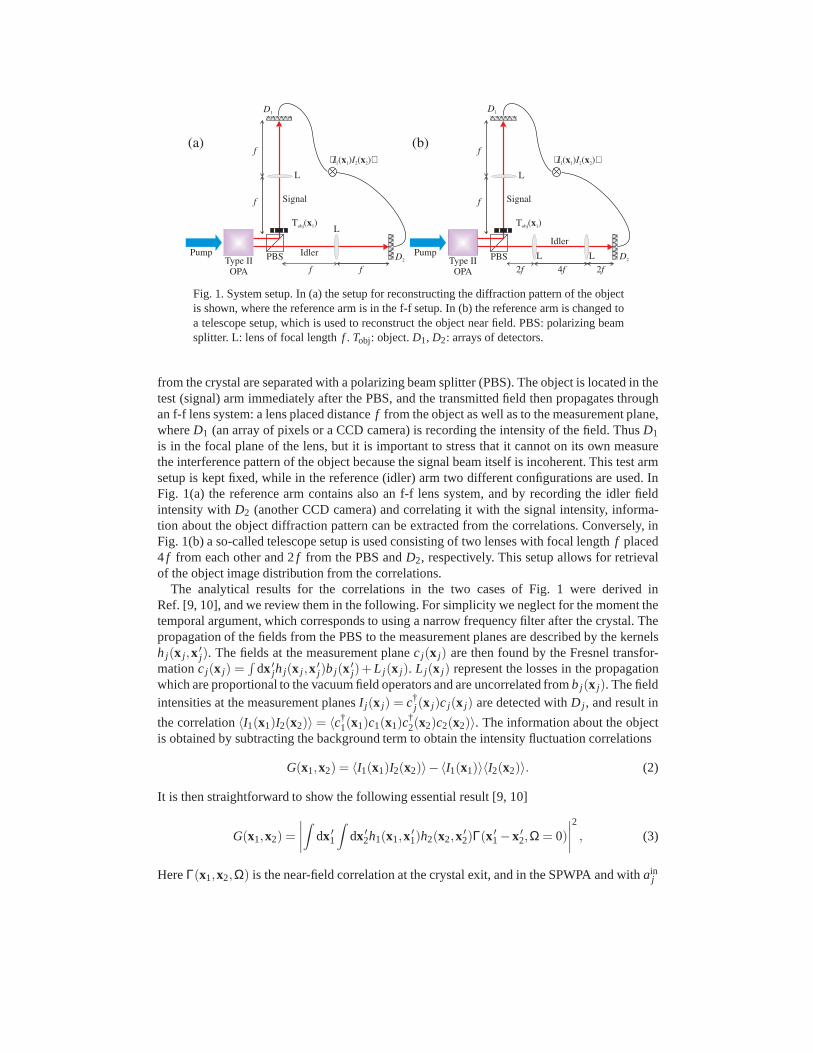
Fig. 1. System setup. In (a) the setup for reconstructing thediffraction pattern of the objectis shown, where the reference arm is in the f-f setup. In (b) the reference arm is changed toa telescope setup, which is used to reconstruct the object near field. PBS: polarizing beamsplitter. L: lens of focal lengthf . Tobj: object.D1, D2: arrays of detectors.

from the crystal are separated with a polarizing beam splitter (PBS). The object is located in thetest (signal) arm immediately after the PBS, and the transmitted field then propagates throughan f-f lens system: a lens placed distancef from the object as well as to the measurement plane,whereD1 (an array of pixels or a CCD camera) is recording the intensity of the field. ThusD1

is in the focal plane of the lens, but it is important to stressthat it cannot on its own measurethe interference pattern of the object because the signal beam itself is incoherent. This test armsetup is kept fixed, while in the reference (idler) arm two different configurations are used. InFig. 1(a) the reference arm contains also an f-f lens system,and by recording the idler fieldintensity withD2 (another CCD camera) and correlating it with the signal intensity, informa-tion about the object diffraction pattern can be extracted from the correlations. Conversely, inFig. 1(b) a so-called telescope setup is used consisting of two lenses with focal lengthf placed4 f from each other and 2f from the PBS andD2, respectively. This setup allows for retrievalof the object image distribution from the correlations.

The analytical results for the correlations in the two casesof Fig. 1 were derived inRef. [9, 10], and we review them in the following. For simplicity we neglect for the moment thetemporal argument, which corresponds to using a narrow frequency filter after the crystal. Thepropagation of the fields from the PBS to the measurement planes are described by the kernelsh j(x j ,x ′

j). The fields at the measurement planec j(x j) are then found by the Fresnel transfor-mationc j(x j) =

∫

dx ′jh j(x j ,x ′

j)b j(x ′j)+L j (x j). L j(x j) represent the losses in the propagation

which are proportional to the vacuum field operators and are uncorrelated fromb j(x j). The fieldintensities at the measurement planesI j(x j) = c†

j (x j)c j(x j) are detected withD j , and result in

the correlation〈I1(x1)I2(x2)〉 = 〈c†1(x1)c1(x1)c

†2(x2)c2(x2)〉. The information about the object

is obtained by subtracting the background term to obtain theintensity fluctuation correlations

G(x1,x2) = 〈I1(x1)I2(x2)〉− 〈I1(x1)〉〈I2(x2)〉. (2)

It is then straightforward to show the following essential result [9, 10]

G(x1,x2) =

∣

∣

∣

∣

∫

dx ′1

∫

dx ′2h1(x1,x ′

1)h2(x2,x ′2)Γ(x ′

1−x ′2,Ω = 0)

∣

∣

∣

∣

2

, (3)

HereΓ(x1,x2,Ω) is the near-field correlation at the crystal exit, and in the SPWPA and withainj

in the vacuum state it is found from Eq. (1) as

Γ(x1,x2,Ω) ≡

∫

dτe−iΩτ〈b1(x1,t1)b2(x2,t1 + τ)〉 =

∫

dq(2π)2 eiq·(x1−x2)γ(q,Ω) , (4)

where we have introduced the gain functionγ(q,Ω) = U1(q,Ω)V2(−q,−Ω). Since Eq. (4)is a function ofx1 − x2 (because of the SPWPA) we will use the notationΓ(x1 − x2,Ω) =Γ(x1,x2,Ω) in the following.

We should mention that when temporal argument is taken into account, Eq. (3) is nolonger valid. We consider the intensities averaged over thedetection timeTD as I j(x j) =

T−1D

∫

TDdtc†

j (x j , t)c j(x j , t). WhenTD is much larger than the coherence time of the sourceτcoh

(which for PDC is typically the case) the following expression holds instead [11]

G(x1,x2) =1

TD

∫

dΩ2π

∣

∣

∣

∣

∫

dx ′1

∫

dx ′2h1(x1,x ′

1)h2(x2,x ′2)Γ(x ′

1−x ′2,Ω)

∣

∣

∣

∣

2

. (5)

This form will be used later for comparing with the numerics.We fix the test arm once and for all as shown in Fig. 1, soh1(x1,x ′

1) ∝ e−ix1·x ′1k/ f Tobj(x ′

1),wherek is the free space wave number of the degenerate down-converted fields. To extractinformation about the diffraction pattern the reference arm is set in the f-f setup of Fig. 1(a),h2(x2,x ′

2) ∝ e−ix2·x ′2k/ f , and Eq. (3) then straightforwardly implies the correlation [9, 10, 11]

Gf(x1,x2) ∝∣

∣γ(−x2k/ f ,Ω = 0) Tobj [(x1 + x2)k/ f ]∣

∣

2, (6)

whereTobj(q) =∫ dx

2π e−iq·xTobj(x) is the amplitude of the object diffraction pattern. The sub-script “f” denotes that the reference arm is in the f-f configuration. The correlation providesinformation about the diffraction pattern of the object if we fix x1 and scanx2, but since thegain also depends onx2 there is a limit to the information we can extract. Precisely, the gainγ(−x2k/ f ,Ω = 0) introduces a cutoff of the reproduced spatial Fourier frequencies at a certaincharacteristic value which we denoteδqPDC; the imaging bandwidthof the PDC source.

We will now show how to circumvent this source-related limitation on the imaging band-width. As previously shown [12] we may in a suitable way average over the position of the testarm detectorx1: First, a change of variables is introduced asx ≡ x1 + x2, and then an averageoverx1 is performed. We then obtain

Gf,SA(x) ≡

∫

dx1Gf(x1,x−x1) ∝∫

dx1∣

∣γ[(x1−x)k/ f ,Ω = 0] Tobj(xk/ f )∣

∣

2

= |Tobj(xk/ f )|2∫

dx1 |γ[(x1−x)k/ f ,Ω = 0]|2 ≃ const×|Tobj(xk/ f )|2 (7)

where the subscript “SA” indicates that a spatial average has been carried out. The final approx-imation in (7) is that|γ(q,Ω = 0)|2 is a bound function inside the detection range ofx1 implyingthat the integral evaluates to a constant. Thus, there is nowno gain cutoff of the diffraction pat-tern, so the imaging bandwidth becomes practically infinite(apart from limitations arising fromthe finite size of the optical elements).1 Note that this average overx1 does not correspond toD1 being a bucket detector. Instead, the change in variablesx ≡ x1 + x2 implies that the spa-tial averaging technique is a convolution of the signal and idler intensity fluctuations, which inpractice is easily calculated using fast Fourier transformtechniques.

1We should mention that whenx is taken to the boundary of the detection range, the integralis no longer a constant.Thus at the boundaries the bandwidth slowly dies out, but it is a quite small effect only affecting a range ofδqPDCthere. In our numerical simulations we use periodic boundary conditions, so this limit does not come into play.

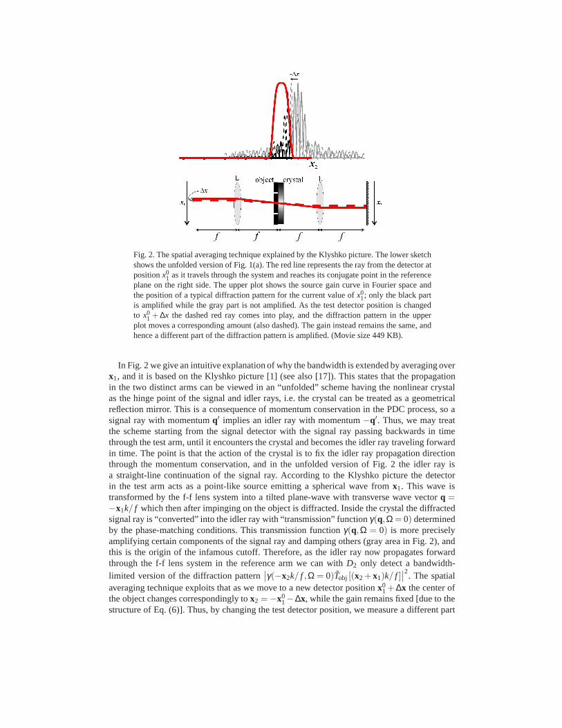
Fig. 2. The spatial averaging technique explained by the Klyshko picture. The lower sketchshows the unfolded version of Fig. 1(a). The red line represents the ray from the detector atpositionx0

1 as it travels through the system and reaches its conjugate point in the referenceplane on the right side. The upper plot shows the source gain curve in Fourier space andthe position of a typical diffraction pattern for the current value ofx0

1; only the black partis amplified while the gray part is not amplified. As the test detector position is changedto x0

1 + ∆x the dashed red ray comes into play, and the diffraction pattern in the upperplot moves a corresponding amount (also dashed). The gain instead remains the same, andhence a different part of the diffraction pattern is amplified. (Movie size 449 KB).

In Fig. 2 we give an intuitive explanation of why the bandwidth is extended by averaging overx1, and it is based on the Klyshko picture [1] (see also [17]). This states that the propagationin the two distinct arms can be viewed in an “unfolded” schemehaving the nonlinear crystalas the hinge point of the signal and idler rays, i.e. the crystal can be treated as a geometricalreflection mirror. This is a consequence of momentum conservation in the PDC process, so asignal ray with momentumq′ implies an idler ray with momentum−q′. Thus, we may treatthe scheme starting from the signal detector with the signalray passing backwards in timethrough the test arm, until it encounters the crystal and becomes the idler ray traveling forwardin time. The point is that the action of the crystal is to fix theidler ray propagation directionthrough the momentum conservation, and in the unfolded version of Fig. 2 the idler ray isa straight-line continuation of the signal ray. According to the Klyshko picture the detectorin the test arm acts as a point-like source emitting a spherical wave fromx1. This wave istransformed by the f-f lens system into a tilted plane-wave with transverse wave vectorq =−x1k/ f which then after impinging on the object is diffracted. Inside the crystal the diffractedsignal ray is “converted” into the idler ray with “transmission” functionγ(q,Ω = 0) determinedby the phase-matching conditions. This transmission function γ(q,Ω = 0) is more preciselyamplifying certain components of the signal ray and dampingothers (gray area in Fig. 2), andthis is the origin of the infamous cutoff. Therefore, as the idler ray now propagates forwardthrough the f-f lens system in the reference arm we can withD2 only detect a bandwidth-limited version of the diffraction pattern

∣

∣γ(−x2k/ f ,Ω = 0)Tobj [(x2 + x1)k/ f ]∣

∣

2. The spatial

averaging technique exploits that as we move to a new detector positionx01 + ∆x the center of

the object changes correspondingly tox2 = −x01−∆x, while the gain remains fixed [due to the

structure of Eq. (6)]. Thus, by changing the test detector position, we measure a different part

of the spatial Fourier spectrum, as shown in Fig. 2. Therefore, by performing a suitable averageas described in Eq. (7) we cover the entire Fourier plane, andeffectively the bandwidth hasbecome unlimited.

Additionally, the spatial averaging technique gives an increased convergence rate of the cor-relation. This is again related to the fact that when the testdetector position is changed fromx0

1 to x01 + ∆x the gain does not change position but the diffraction pattern does. Assuming that

the PDC gain extension is much larger than the extension of a pixel, the shifted diffractionpattern atx0

1 + ∆x overlaps quite substantially with the previous one. Thus, as x1 is scanneda given position of the diffraction pattern has as many independent contributions as there areindependent modes inside the gain bandwidth, which as a goodestimate is given by the ratio ofthe PDC bandwidthδqPDC with the pump bandwidthδqp = 2/w0 [15], wherew0 is the pumpwaist. A measure of the speedup in the correlation convergence in each transverse dimension istherefore given by

ρSA = δqPDC/δqp. (8)

In the simulations shown later concerning the convergence rate, we used a temporal grid thatcorresponds to a 22 nm interference filter. In that caseδqPDC ≃ 6q0, whereq0 =

√

k/lc is thenatural bandwidth of PDC at a given temporal frequency [15].The pump size in the numericswas chosen soδqp = q0/18 (corresponding to a pump size of 600µm), implying we shouldexpect a convergence rate speedup ofρSA ≃ 102.

Note that instead of fixingx1 and scanningx2, we may scanx1 and fixx2. In this case Eq. (6)reveals that the gain no longer limits the imaging bandwidth, and therefore it is in principlenot necessary to do a spatial average to overcome the gain limitation. The physical explanationbehind this is again found from the Klyshko picture: fixingx2 at a suitable position (i.e. at theposition of maximum gain, cf. Fig. 2), scanningx1 will move the diffraction pattern seen at thisposition over the whole range giving an unlimited imaging bandwidth. However, scanningx1

and fixingx2 does not benefit of the improved convergence. To achieve thisa spatial averageshould be done, whereby the method amounts to the same operation as described previously.

Let us now turn to the problem of reconstructing the object image. Keeping the test arm fixedand changing the reference arm to the telescope setup [see Fig. 1(b)],h2(x2,x ′

2) = δ (x2− x ′2)

and Eq. (3) becomes [9, 10, 11]

GT(x1,x2) ∝∣

∣

∣

∣

∫

dx ′1Γ(x ′

1−x2,Ω = 0)Tobj(

x ′1

)

e−ix ′1·x1k/ f

∣

∣

∣

∣

2

(9)

≈ |Tobj(x2)|2 |γ (x1k/ f ,Ω = 0)|2 . (10)

Thus, fixingx1 the object can be observed by scanningx2. The approximation that leads toEq. (10) holds as long as the smallest length scale of the object is larger than the coherencelength xcoh of Γ(x ′

1 − x2,Ω = 0). This is becauseΓ(x ′1 − x2,Ω = 0) is nonzero in a region

of the sizexcoh aroundx ′1 = x2 and thusTobj changes slowly with respect to this function

and may consequently be pulled out of the integration. In general, Eq. (9) is a convolutionbetween the correlation function and the object, and hence the width xcoh of the near-fieldcorrelation functionΓ(x ′

1 − x2,Ω = 0) determines the resolution of the reconstructed image,and has typically a value ofxcoh = 1/q0.

In reconstructing the image a technique corresponding to the spatial average done for recon-structing the diffraction pattern would result in a largelyincreased image resolution. Unfortu-nately, it is not possible to carry out such a spatial averageto achieve this. However, if we makea simple sum over all the positions ofD1 (corresponding toD1 being a bucket detector), instead

of Eq. (9) we have the following exact expression2

GT(x2) =∫

dx1GT(x1,x2) ∝∫

dx1|Γ(x1−x2,Ω = 0)|2|Tobj(x1) |2, (11)

where the bar denotes thatD1 is a bucket detector and therefore thatx1 has been integratedout. Eq. (11) has the form of an incoherent imaging scheme, while Eq. (9) has the form of acoherent imaging scheme (the same conclusion – that using a bucket detector can make theimaging incoherent – was reached in Ref. [8] in the low-gain regime). As we shall see later, theincoherent form has both advantages and drawbacks comparedto the coherent case.

3. Numerical examples

The imaging performance of the system was checked through numerical simulations of themodel described in detail in Ref. [15]. It includes spatial and temporal dispersion up to secondorder, as well as a Gaussian shape in space and time of the pumpbeam. The simulations with1 transverse dimension (1D) were calculated including the temporal argument (using a grid ofNx = 512 andNt = 64), while the ones with 2 transverse dimensions (2D) had a more qualitativenature since they neglected the time argument (a grid ofNx = Ny = 256 was used).3 Eachpump shot was propagated along the crystal inNz = 200 steps. The Gaussian pump profilehad a waistw0 = 600 µm and a duration ofτ0 = 1.5 ps, and the other parameters were asin [12, 15] chosen to closely mimic that of anlc = 4 mm long BBO crystal used in a currentexperiment in Como [14]. The characteristic space and time units of the PDC source arexcoh=1/q0 ≃ 16 µm andτcoh = 1/Ω0 ≃ 0.96 ps. The pulsed character of the pump is importantbecause typically the CCD cameras used in experiments have very slow response times. Ifthe measurement time becomes too long with respect toτcoh, the visibility of the correlationbecomes very poor (see also Refs. [6, 10, 11]). This only affects the case when the intensity isdetected in the high gain regime, i.e. when the background term in Eq. (2) is substantial, while itdoes not affect the coincidence counting regime or the case when homodyne measurements areperformed as in Ref. [12]. Note that in the telescope setup the performance was optimized bytaking the imaging plane of the telescope setup inside the crystal by the amount∆z=−(1/n1+1/n2) tanh(σplc)/σp [12, 15], wheren j are the refractive indices, andσp is a gain parameter. Inthis way, the quadratic phase dependence of the gain is cancelled. For more technical details onthis and the numerics we refer to Refs. [12, 15].

Let us show quantitatively how the object diffraction pattern is reconstructed by using adouble slit as an object in the setup of Fig. 1(a). The correlations as calculated in 1D bothwith and without the spatial average are presented in Fig. 3(a)-(b). The correlation withoutspatial average in (a) clearly suffers from a limited bandwidth, and from the animation a slowconvergence rate is evident. In contrast, the correlation with spatial average in (b) is able toreproduce the entire spectrum of the diffraction pattern and after much fewer repeated pumpshots. To check the convergence rate, we have calculated theroot-mean-squared error of thecorrelationGn

f (after averaging overn number of shots) relative to the analytically calculatedcorrelationGf . Gf was calculated by using semi-analytical methods includingthe analyticalSPWPA gain as well as integrating over time [see Eq. (5)]. Theerror is then evaluated as

εf(n) =(

Σx|Gnf (x)−Gf(x)|2

)1/2(12)

2The expression is exact because no approximations have beenmade about object length scales vs.xcoh.3This was done to save CPU time since many thousands of repeated pump shots were needed for the correlations

to converge, and corresponds to using a narrow bandwidth interference filter after the crystal. In fact, the temporal gridacts just as an interference filter by providing a cutoff in frequency space. In the simulations with time the cutoff waschosen so it corresponds to having a 22 nm interference filterafter the BBO crystal, while the simulations neglectingtime are equivalent to placing a< 1 nm interference filter after the crystal.

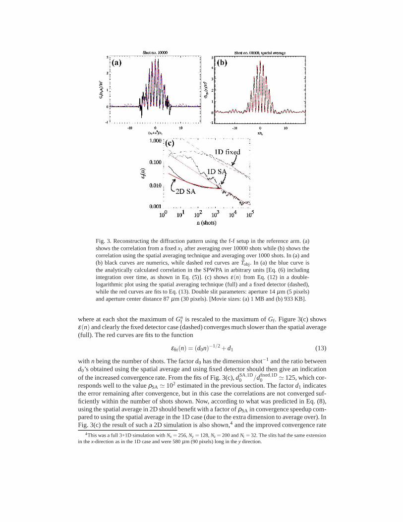
Fig. 3. Reconstructing the diffraction pattern using the f-f setup in the reference arm. (a)shows the correlation from a fixedx1 after averaging over 10000 shots while (b) shows thecorrelation using the spatial averaging technique and averaging over 1000 shots. In (a) and(b) black curves are numerics, while dashed red curves areTobj. In (a) the blue curve isthe analytically calculated correlation in the SPWPA in arbitrary units [Eq. (6) includingintegration over time, as shown in Eq. (5)]. (c) showsε(n) from Eq. (12) in a double-logarithmic plot using the spatial averaging technique (full) and a fixed detector (dashed),while the red curves are fits to Eq. (13). Double slit parameters: aperture 14µm (5 pixels)and aperture center distance 87µm (30 pixels). [Movie sizes: (a) 1 MB and (b) 933 KB].

where at each shot the maximum ofGnf is rescaled to the maximum ofGf . Figure 3(c) shows

ε(n) and clearly the fixed detector case (dashed) converges much slower than the spatial average(full). The red curves are fits to the function

εfit(n) = (d0n)−1/2 +d1 (13)

with n being the number of shots. The factord0 has the dimension shot−1 and the ratio betweend0’s obtained using the spatial average and using fixed detector should then give an indicationof the increased convergence rate. From the fits of Fig. 3(c),dSA,1D

0 /dfixed,1D0 ≃ 125, which cor-

responds well to the valueρSA ≃ 102 estimated in the previous section. The factord1 indicatesthe error remaining after convergence, but in this case the correlations are not converged suf-ficiently within the number of shots shown. Now, according towhat was predicted in Eq. (8),using the spatial average in 2D should benefit with a factor ofρSA in convergence speedup com-pared to using the spatial average in the 1D case (due to the extra dimension to average over). InFig. 3(c) the result of such a 2D simulation is also shown,4 and the improved convergence rate

4This was a full 3+1D simulation withNx = 256,Ny = 128,Nz = 200 andNt = 32. The slits had the same extensionin thex-direction as in the 1D case and were 580µm (90 pixels) long in they direction.

of the 2D simulation is evident: from the fitsdSA,2D0 /dSA,1D

0 ≃ 73, again corresponding well tothe predicted estimate ofρSA ≃ 102. A minor problem in this comparison is that the 2D resultssaturate very quickly to a rather high error level of 1%, while the 1D results go as low as 0.1%.This difference turned out to be caused by the Gaussian shapeof the pump field and the objectextension; the object is very localized in thex direction and therefore we get a low error ratein the 1D case. However, in the 2D case the object is quite extended in they direction and theaverage error reported in theε value is therefore higher. This quick saturation in 2D gave somenumerical problems in fitting well the data to Eq. (13), so thed0 value obtained should be takencautiously. However, there is no doubt about the main point:going from 1D to 2D the spatialaveraging technique speeds further up.

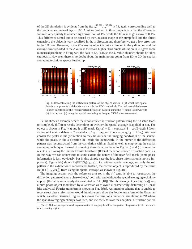
Fig. 4. Reconstructing the diffraction pattern of the object shown in (a) which has spatialFourier components both inside and outside the PDC bandwidth. The real part of the inverseFourier transform of the reconstructed diffraction pattern using the f-f setup is shown with(b) fixedx1 and (c) using the spatial averaging technique. 35000 shots were used.

Let us show an example where the reconstructed diffraction pattern using the f-f setup leadsto completely different results depending on whether the spatial average is applied or not. Theobject is shown in Fig. 4(a) and is a 2D maskTobj(x) = [1+ cos(xq0)][1+ cos(3yq0)]/4 (con-sisting of 4 main sidebands, 2 located atq/q0 = ±ex and 2 located atq/q0 = ±3ey). We havechosen the peaks in they-direction so they lie outside the imaging bandwidth of the source,while the peaks in thex-direction lie inside the bandwidth. In the numerics the diffractionpattern was reconstructed from the correlation withx1 fixed as well as employing the spatialaveraging technique. Instead of showing these data, we havein Fig. 4(b) and (c) shown theresults after taking the inverse Fourier transform (IFT) ofthe reconstructed diffraction patterns.In this way we can reconstruct to some extend the nature of thenear field mask (some phaseinformation is lost, obviously, but in this simple case the lost phase information is not so im-portant). Figure 4(b) shows Re(IFT[Gf(x1,x2)]), i.e. without spatial average, and only the rollpattern in thex-direction is reproduced. Instead, the correct object is reproduced by the resultRe(IFT[Gf,SA(x)]) from using the spatial average, as shown in Fig. 4(c).

The imaging system with the reference arm set in the f-f setupis able to reconstruct thediffraction pattern of a pure phase object,5 both with and without the spatial averaging techniqueapplied (the latter was already demonstrated in Ref. [10]).The chosen object [see Fig. 5(a)] wasa pure phase object modulated by a Gaussian as to avoid a cosmetically disturbing DC peak[the analytical Fourier transform is shown in Fig. 5(b)]. Animaging scheme that is unable toreconstruct phase information would therefore only show the Fourier transform of the Gaussianwhich is another Gaussian. Figure 5(c) shows the result of a numerical simulation in 2D wherethe spatial averaging technique was used, and it closely follows the analytical diffraction pattern

5Ref. [18] shows an experimental implementation of imaging the diffraction pattern of a phase object in the coinci-dence counting regime.

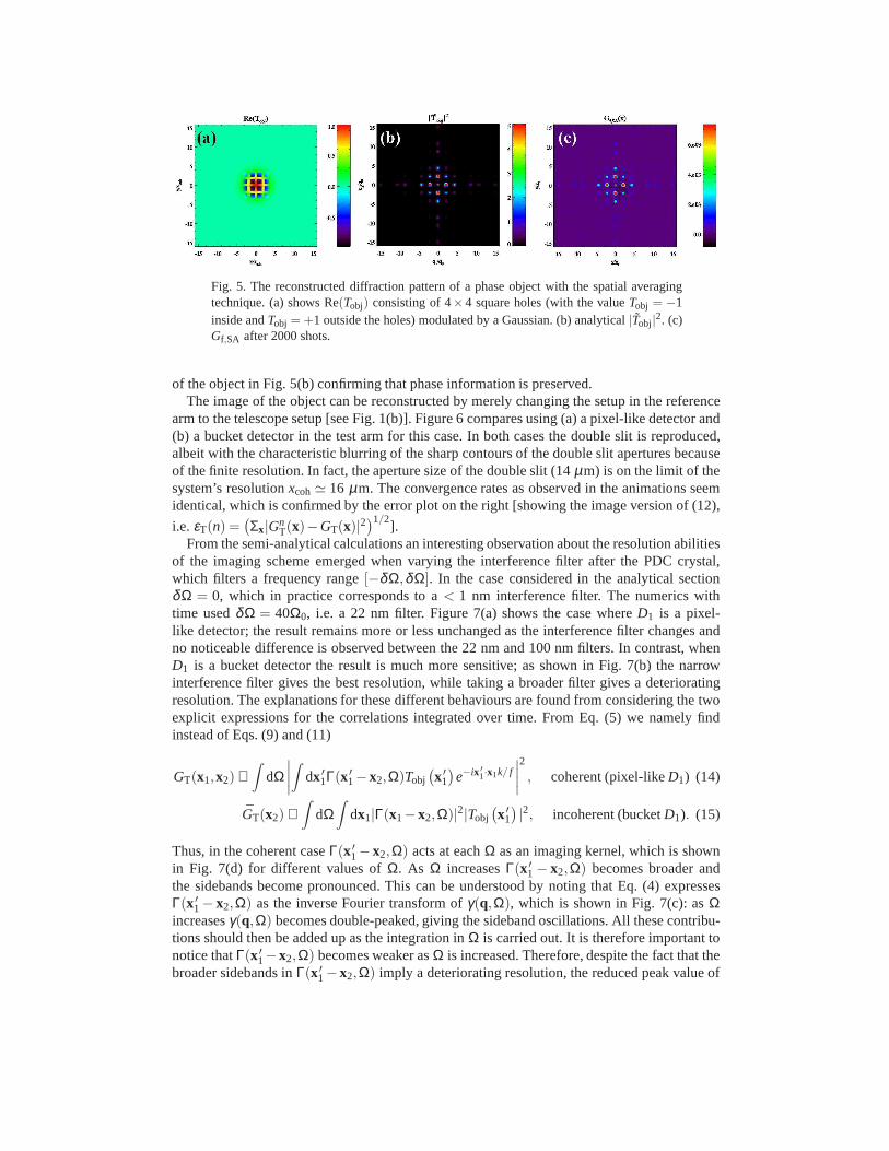
Fig. 5. The reconstructed diffraction pattern of a phase object with the spatial averagingtechnique. (a) shows Re(Tobj) consisting of 4×4 square holes (with the valueTobj = −1inside andTobj = +1 outside the holes) modulated by a Gaussian. (b) analytical|Tobj|

2. (c)Gf,SA after 2000 shots.

of the object in Fig. 5(b) confirming that phase information is preserved.The image of the object can be reconstructed by merely changing the setup in the reference

arm to the telescope setup [see Fig. 1(b)]. Figure 6 comparesusing (a) a pixel-like detector and(b) a bucket detector in the test arm for this case. In both cases the double slit is reproduced,albeit with the characteristic blurring of the sharp contours of the double slit apertures becauseof the finite resolution. In fact, the aperture size of the double slit (14µm) is on the limit of thesystem’s resolutionxcoh≃ 16 µm. The convergence rates as observed in the animations seemidentical, which is confirmed by the error plot on the right [showing the image version of (12),

i.e. εT(n) =(

Σx|GnT(x)−GT(x)|2

)1/2].

From the semi-analytical calculations an interesting observation about the resolution abilitiesof the imaging scheme emerged when varying the interferencefilter after the PDC crystal,which filters a frequency range[−δΩ,δΩ]. In the case considered in the analytical sectionδΩ = 0, which in practice corresponds to a< 1 nm interference filter. The numerics withtime usedδΩ = 40Ω0, i.e. a 22 nm filter. Figure 7(a) shows the case whereD1 is a pixel-like detector; the result remains more or less unchanged as the interference filter changes andno noticeable difference is observed between the 22 nm and 100 nm filters. In contrast, whenD1 is a bucket detector the result is much more sensitive; as shown in Fig. 7(b) the narrowinterference filter gives the best resolution, while takinga broader filter gives a deterioratingresolution. The explanations for these different behaviours are found from considering the twoexplicit expressions for the correlations integrated overtime. From Eq. (5) we namely findinstead of Eqs. (9) and (11)

GT(x1,x2) ∝∫

dΩ∣

∣

∣

∣

∫

dx ′1Γ(x ′

1−x2,Ω)Tobj(

x ′1

)

e−ix ′1·x1k/ f

∣

∣

∣

∣

2

, coherent (pixel-likeD1) (14)

GT(x2) ∝∫

dΩ∫

dx1|Γ(x1−x2,Ω)|2|Tobj(

x ′1

)

|2, incoherent (bucketD1). (15)

Thus, in the coherent caseΓ(x ′1− x2,Ω) acts at eachΩ as an imaging kernel, which is shown

in Fig. 7(d) for different values ofΩ. As Ω increasesΓ(x ′1 − x2,Ω) becomes broader and

the sidebands become pronounced. This can be understood by noting that Eq. (4) expressesΓ(x ′

1 − x2,Ω) as the inverse Fourier transform ofγ(q,Ω), which is shown in Fig. 7(c): asΩincreasesγ(q,Ω) becomes double-peaked, giving the sideband oscillations.All these contribu-tions should then be added up as the integration inΩ is carried out. It is therefore important tonotice thatΓ(x ′

1−x2,Ω) becomes weaker asΩ is increased. Therefore, despite the fact that thebroader sidebands inΓ(x ′

1−x2,Ω) imply a deteriorating resolution, the reduced peak value of

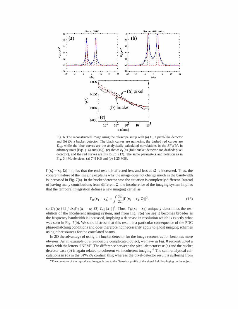
Fig. 6. The reconstructed image using the telescope setup with (a)D1 a pixel-like detectorand (b)D1 a bucket detector. The black curves are numerics, the dashedred curves areTobj, while the blue curves are the analytically calculated correlations in the SPWPA inarbitrary units [Eqs. (14) and (15)]. (c) showsεT(n) (full: bucket detector and dashed: pixeldetector), and the red curves are fits to Eq. (13). The same parameters and notation as inFig. 3. [Movie sizes: (a) 748 KB and (b) 1.25 MB].

Γ(x ′1− x2,Ω) implies that the end result is affected less and less asΩ is increased. Thus, the

coherent nature of the imaging explains why the image does not change much as the bandwidthis increased in Fig. 7(a). In the bucket detector case the situation is completely different. Insteadof having many contributions from differentΩ, the incoherence of the imaging system impliesthat the temporal integration defines a new imaging kernel as

ΓB(x1−x2) ≡

∫

dΩ2π

|Γ(x1−x2,Ω)|2. (16)

so GT(x2) ∝∫

dx1ΓB(x1− x2,Ω)|Tobj(x1) |2. Thus,ΓB(x1− x2) uniquely determines the res-

olution of the incoherent imaging system, and from Fig. 7(e)we see it becomes broader asthe frequency bandwidth is increased, implying a decrease in resolution which is exactly whatwas seen in Fig. 7(b). We should stress that this result is a particular consequence of the PDCphase-matching conditions and does therefore not necessarily apply to ghost imaging schemesusing other sources for the correlated beams.

In 2D the advantage of using the bucket detector for the imagereconstruction becomes moreobvious. As an example of a reasonably complicated object, we have in Fig. 8 reconstructed amask with the letters “INFM”. The difference between the pixel-detector case (a) and the bucketdetector case (b) is again related to coherent vs. incoherent imaging.6 The semi-analytical cal-culations in (d) in the SPWPA confirm this; whereas the pixel-detector result is suffering from

6The curvature of the reproduced images is due to the Gaussianprofile of the signal field impinging on the object.

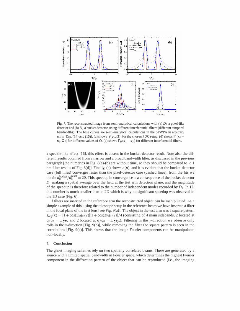
Fig. 7. The reconstructed image from semi-analytical calculations with (a)D1 a pixel-likedetector and (b)D1 a bucket detector, using different interferential filters (different temporalbandwidths). The blue curves are semi-analytical calculations in the SPWPA in arbitraryunits [Eqs. (14) and (15)]. (c) shows|γ(qx,Ω)| for the chosen PDC setup. (d) shows|Γ(x1−x2,Ω)| for different values ofΩ. (e) showsΓB(x1−x2) for different interferential filters.

a speckle-like effect [16], this effect is absent in the bucket-detector result. Note also the dif-ferent results obtained from a narrow and a broad bandwidth filter, as discussed in the previousparagraph [the numerics in Fig. 8(a)-(b) are without time, so they should be compared to< 1nm filter results of Fig. 8(d)]. Finally, (c) showsε(n), and it is evident that the bucket-detectorcase (full lines) converges faster than the pixel-detectorcase (dashed lines); from the fits weobtaindbucket

0 /dpixel0 ≃ 20. This speedup in convergence is a consequence of the bucket detector

D1 making a spatial average over the field at the test arm detection plane, and the magnitudeof the speedup is therefore related to the number of independent modes recorded byD1. In 1Dthis number is much smaller than in 2D which is why no significant speedup was observed inthe 1D case (Fig. 6).

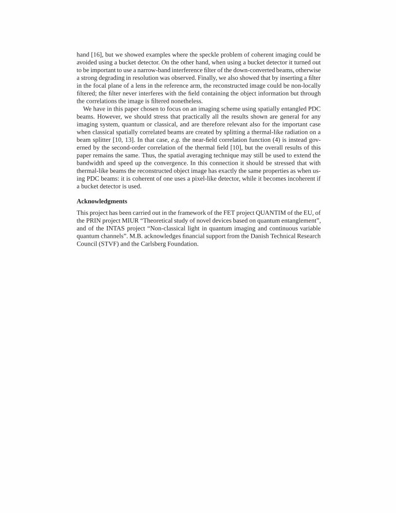
If filters are inserted in the reference arm the reconstructed object can be manipulated. As asimple example of this, using the telescope setup in the reference beam we have inserted a filterin the focal plane of the first lens [see Fig. 9(a)]. The objectin the test arm was a square patternTobj(x) = [1+ cos(3xq0/2)][1+ cos(3yq0/2)]/4 (consisting of 4 main sidebands, 2 located atq/q0 = ± 3

2ex and 2 located atq/q0 = ± 32ey.). Filtering in they-direction we observe only

rolls in thex-direction [Fig. 9(b)], while removing the filter the squarepattern is seen in thecorrelations [Fig. 9(c)]. This shows that the image Fouriercomponents can be manipulatednon-locally.

4. Conclusion

The ghost imaging schemes rely on two spatially correlated beams. These are generated by asource with a limited spatial bandwidth in Fourier space, which determines the highest Fouriercomponent in the diffraction pattern of the object that can be reproduced (i.e., the imaging

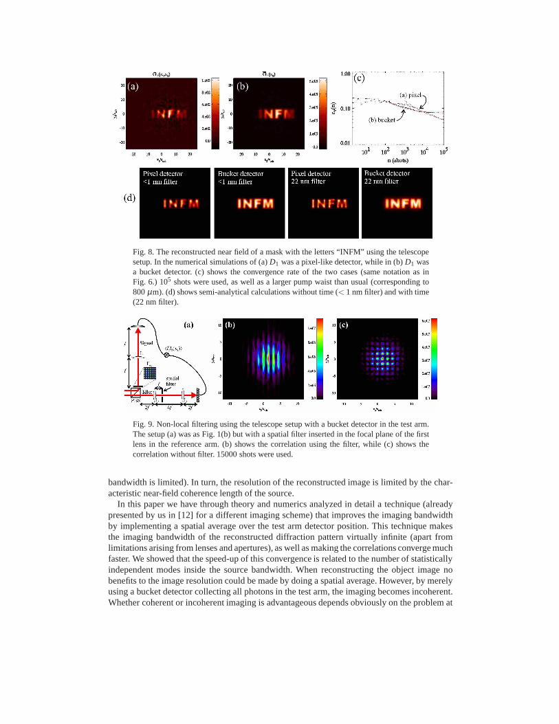
Fig. 8. The reconstructed near field of a mask with the letters“INFM” using the telescopesetup. In the numerical simulations of (a)D1 was a pixel-like detector, while in (b)D1 wasa bucket detector. (c) shows the convergence rate of the two cases (same notation as inFig. 6.) 105 shots were used, as well as a larger pump waist than usual (corresponding to800µm). (d) shows semi-analytical calculations without time (< 1 nm filter) and with time(22 nm filter).

Fig. 9. Non-local filtering using the telescope setup with a bucket detector in the test arm.The setup (a) was as Fig. 1(b) but with a spatial filter inserted in the focal plane of the firstlens in the reference arm. (b) shows the correlation using the filter, while (c) shows thecorrelation without filter. 15000 shots were used.

bandwidth is limited). In turn, the resolution of the reconstructed image is limited by the char-acteristic near-field coherence length of the source.

In this paper we have through theory and numerics analyzed indetail a technique (alreadypresented by us in [12] for a different imaging scheme) that improves the imaging bandwidthby implementing a spatial average over the test arm detectorposition. This technique makesthe imaging bandwidth of the reconstructed diffraction pattern virtually infinite (apart fromlimitations arising from lenses and apertures), as well as making the correlations converge muchfaster. We showed that the speed-up of this convergence is related to the number of statisticallyindependent modes inside the source bandwidth. When reconstructing the object image nobenefits to the image resolution could be made by doing a spatial average. However, by merelyusing a bucket detector collecting all photons in the test arm, the imaging becomes incoherent.Whether coherent or incoherent imaging is advantageous depends obviously on the problem at

hand [16], but we showed examples where the speckle problem of coherent imaging could beavoided using a bucket detector. On the other hand, when using a bucket detector it turned outto be important to use a narrow-band interference filter of the down-converted beams, otherwisea strong degrading in resolution was observed. Finally, we also showed that by inserting a filterin the focal plane of a lens in the reference arm, the reconstructed image could be non-locallyfiltered; the filter never interferes with the field containing the object information but throughthe correlations the image is filtered nonetheless.

We have in this paper chosen to focus on an imaging scheme using spatially entangled PDCbeams. However, we should stress that practically all the results shown are general for anyimaging system, quantum or classical, and are therefore relevant also for the important casewhen classical spatially correlated beams are created by splitting a thermal-like radiation on abeam splitter [10, 13]. In that case,e.g.the near-field correlation function (4) is instead gov-erned by the second-order correlation of the thermal field [10], but the overall results of thispaper remains the same. Thus, the spatial averaging technique may still be used to extend thebandwidth and speed up the convergence. In this connection it should be stressed that withthermal-like beams the reconstructed object image has exactly the same properties as when us-ing PDC beams: it is coherent of one uses a pixel-like detector, while it becomes incoherent ifa bucket detector is used.

Acknowledgments

This project has been carried out in the framework of the FET project QUANTIM of the EU, ofthe PRIN project MIUR “Theoretical study of novel devices based on quantum entanglement”,and of the INTAS project “Non-classical light in quantum imaging and continuous variablequantum channels”. M.B. acknowledges financial support from the Danish Technical ResearchCouncil (STVF) and the Carlsberg Foundation.