Gfdk Course

Introduction to GFDK The Schlumberger GeoFrame Developer’s Kit (GFDK) lets developers build new programs that interoperate with the suite of GeoFrame applications. The kit is very extensive and powerful if used correctly.

Course Overview The Introduction to GFDK course is designed to equip a developer with the tools necessary to use the GFDK effectively. The GFDK is an immense code base spanning the entire GeoFrame source code. Without a little guidance, it can be fairly easy to get lost. This course provides users with the important steps to successfully write their own GFDK programs by explaining various settings and supplying numerous example programs. With the knowledge acquired from this class, each student should be able to take the example programs, compile, link, and run them, as well as make their own GFDK programs. The Introduction to GFDK course specifically covers the following topics:

• GFDK Documentation • Getting around in GeoFrame • Setting up the Development Environment • IESX DK – IESX Data Access • GeoViz On Connect • GFDK Integration

Documentation The GFDK has plenty of relevant documentation, which can be found on the GFDK Bookshelf. While this course uses many of the concepts from each of the documents, only three documents are of particular interest: IESX Data Access, GeoViz On Connect, and GFDK Integration. However, it is encouraged to look at the other documents on the GFDK Bookshelf for your general knowledge, as this course tries to serve as a one-stop shop, which bases itself from the need-to-know concepts in the GFDK Bookshelf documents. So, if you want more information than this class provides, please feel free to peruse the GFDK Bookshelf.

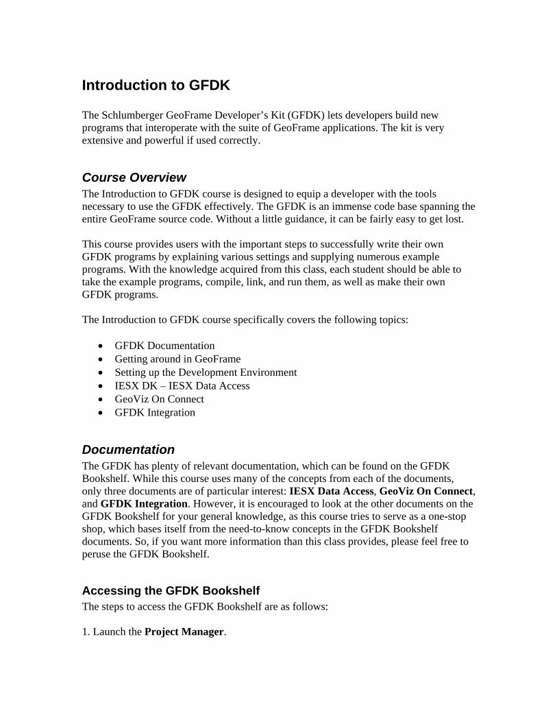
Accessing the GFDK Bookshelf The steps to access the GFDK Bookshelf are as follows: 1. Launch the Project Manager.

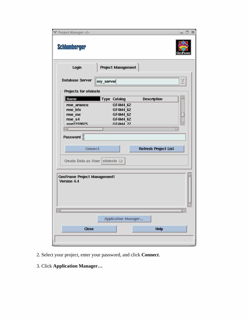
2. Select your project, enter your password, and click Connect. 3. Click Application Manager…

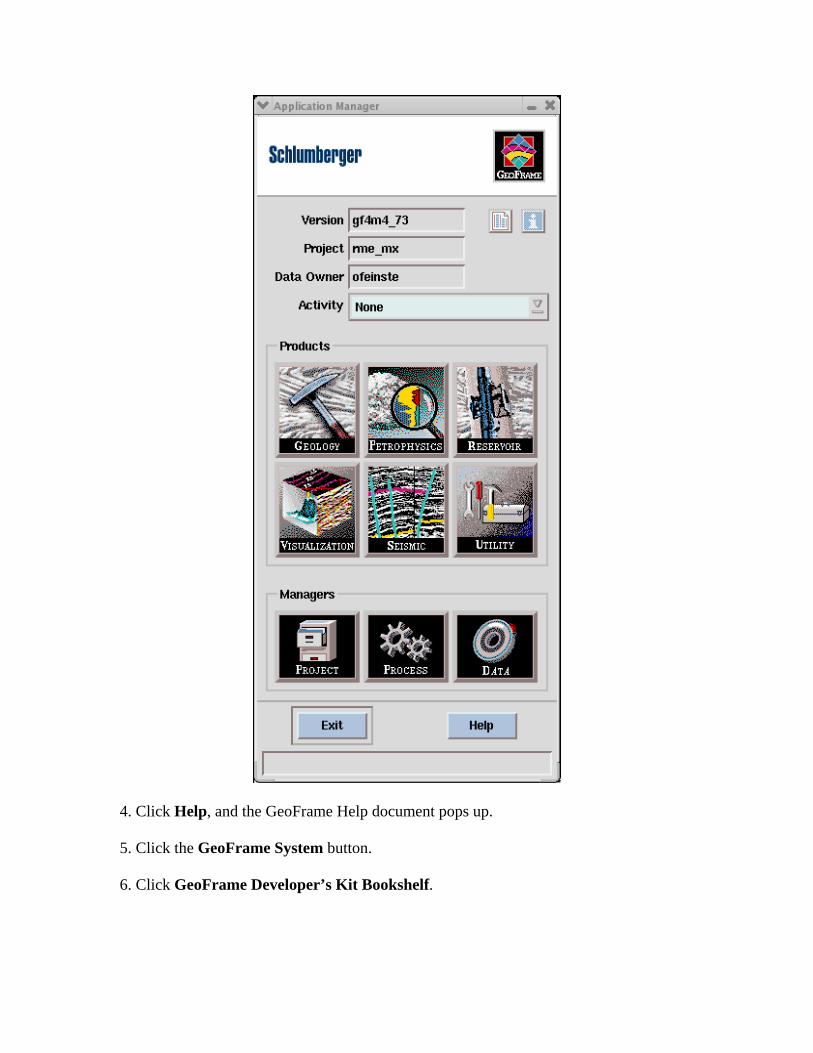
4. Click Help, and the GeoFrame Help document pops up. 5. Click the GeoFrame System button. 6. Click GeoFrame Developer’s Kit Bookshelf.

7. Click on any of the links to access specific GFDK Documentation.

Overview of the GeoFrame architecture

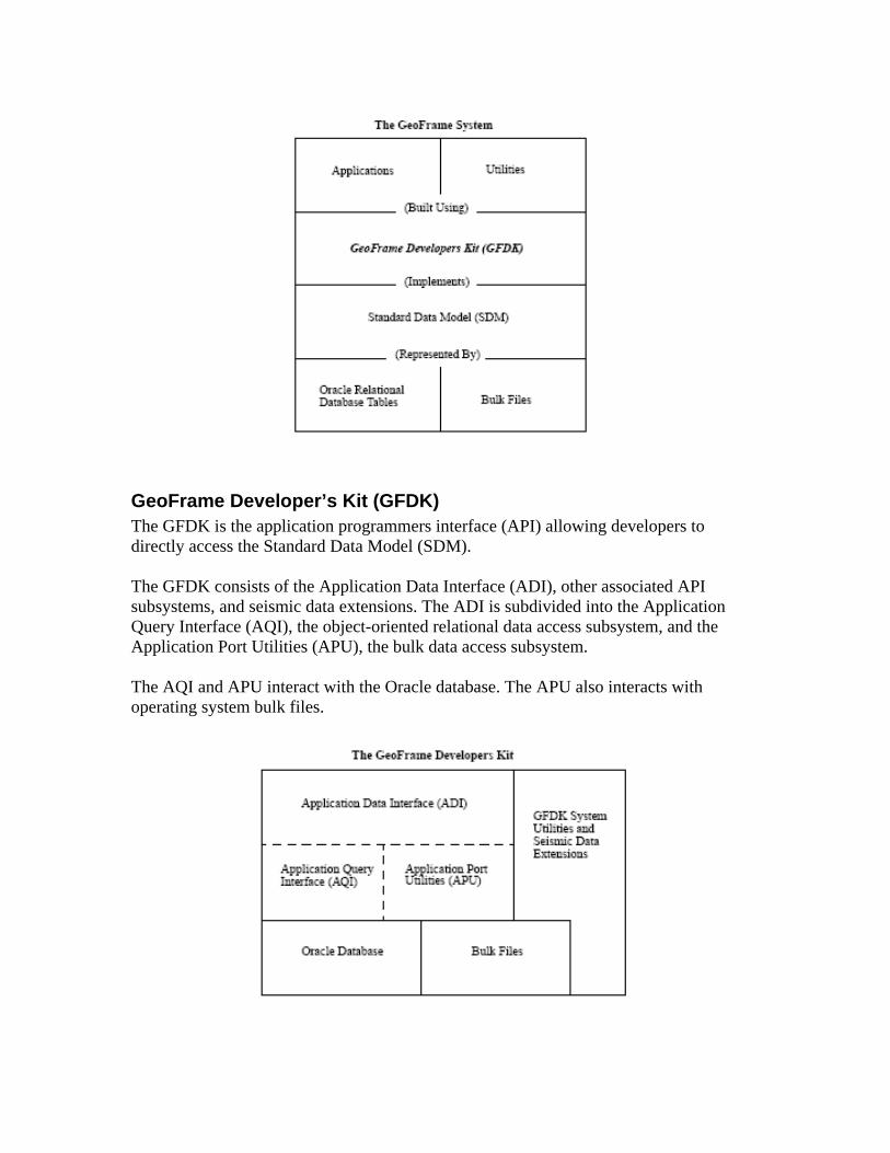
GeoFrame Components The basic components of the GeoFrame system include end-user applications (IESX, Stratlog, Petroview Plus, Charisma, etc.), project and data administration utilities (pm, DLIS Load, etc.), a standard data model (the SDM), and an application programmers interface to the data model (the GFDK API). GeoFrame applications and utilities are built using the GFDK API. The GFDK API, in turn, implements the Standard Data Model, which is represented in the Oracle relational database and related bulk files.

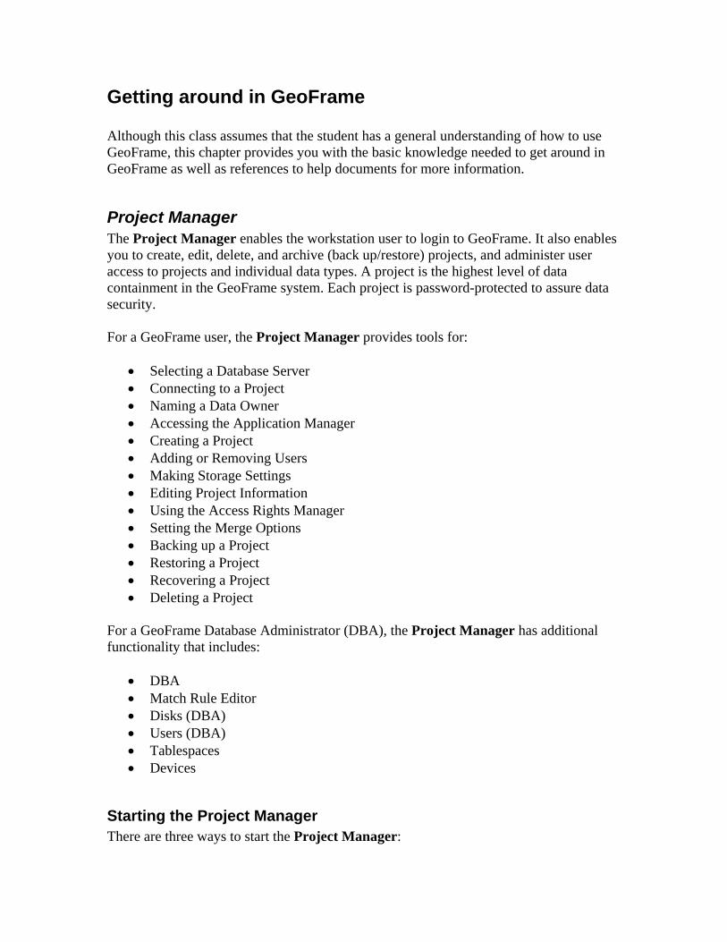
GeoFrame Developer’s Kit (GFDK) The GFDK is the application programmers interface (API) allowing developers to directly access the Standard Data Model (SDM). The GFDK consists of the Application Data Interface (ADI), other associated API subsystems, and seismic data extensions. The ADI is subdivided into the Application Query Interface (AQI), the object-oriented relational data access subsystem, and the Application Port Utilities (APU), the bulk data access subsystem. The AQI and APU interact with the Oracle database. The APU also interacts with operating system bulk files.

Getting around in GeoFrame Although this class assumes that the student has a general understanding of how to use GeoFrame, this chapter provides you with the basic knowledge needed to get around in GeoFrame as well as references to help documents for more information.

Project Manager The Project Manager enables the workstation user to login to GeoFrame. It also enables you to create, edit, delete, and archive (back up/restore) projects, and administer user access to projects and individual data types. A project is the highest level of data containment in the GeoFrame system. Each project is password-protected to assure data security. For a GeoFrame user, the Project Manager provides tools for:

• Selecting a Database Server • Connecting to a Project • Naming a Data Owner • Accessing the Application Manager • Creating a Project • Adding or Removing Users • Making Storage Settings • Editing Project Information • Using the Access Rights Manager • Setting the Merge Options • Backing up a Project • Restoring a Project • Recovering a Project • Deleting a Project

For a GeoFrame Database Administrator (DBA), the Project Manager has additional functionality that includes:

• DBA • Match Rule Editor • Disks (DBA) • Users (DBA) • Tablespaces • Devices

Starting the Project Manager There are three ways to start the Project Manager:

1. Select GeoFrame from the GeoFrame menu on Geonet.

2. Enter proman & in a GeoFrame xterm window.

3. Select the Project icon from the GeoFrame Application Manager window.

Project Manager Reference For more information on the Project Manager, you can click on Project Management User’s Guide in the GFDK Bookshelf.

Process Manager The Process Manager allows you to build and run chains of GeoFrame modules to analyze and interpret your oilfield data. When modules are linked together in chains, the output from one module is input to the next module in the chain. In Process Manager, you can:

• Create a new chain of modules • Modify an existing chain • Use one of the default chains provided, or rename and modify it to suit your needs • Create and save a container – called an activity – for the chain; the activity

becomes part of your database • Set data focus • Generate and execute a script file to automate commonly used procedures • Set the data parameters for a module before you run it • Control the execution of a module

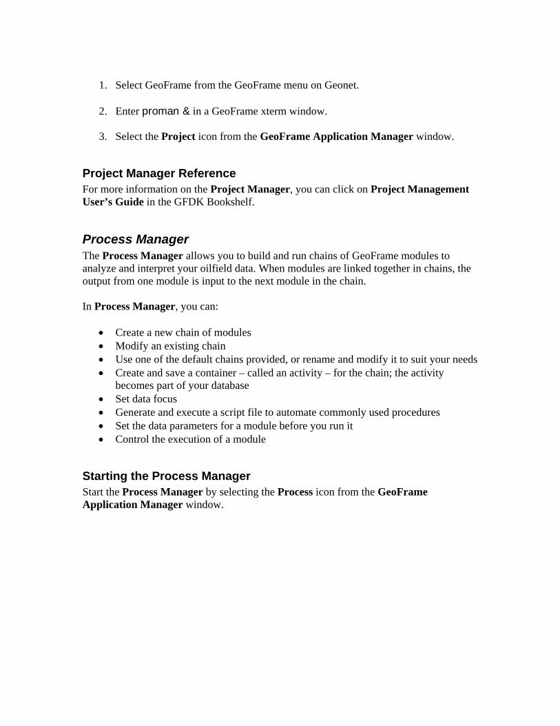
Starting the Process Manager Start the Process Manager by selecting the Process icon from the GeoFrame Application Manager window.

Process Manager Reference For more information on the Process Manager, you can click on Process Manager’s User’s Guide in the GFDK Bookshelf.

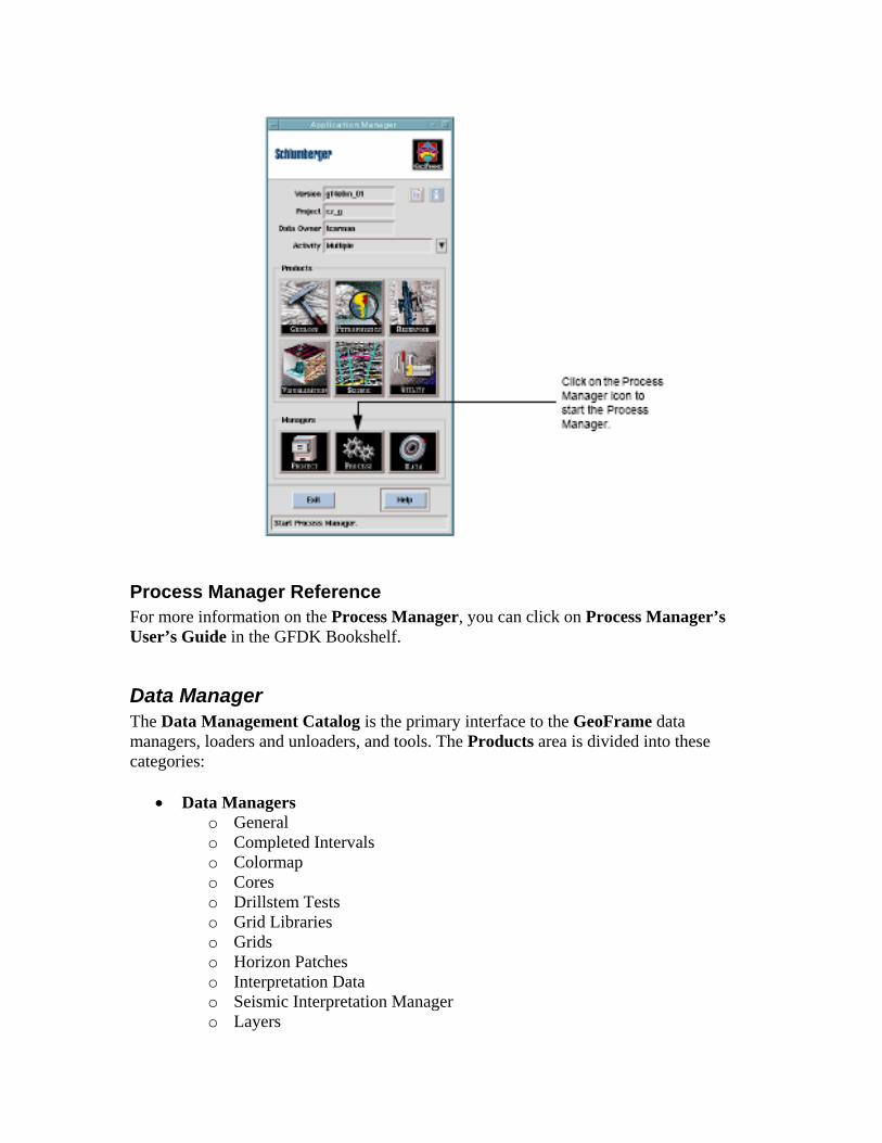
Data Manager The Data Management Catalog is the primary interface to the GeoFrame data managers, loaders and unloaders, and tools. The Products area is divided into these categories:

• Data Managers o General o Completed Intervals o Colormap o Cores o Drillstem Tests o Grid Libraries o Grids o Horizon Patches o Interpretation Data o Seismic Interpretation Manager o Layers

o Litho Zones o Log Curves o Markers o Surfaces o Wells and Boreholes o Zone Versions

• Loaders and Unloaders o ASCII Load o Data Load o Data Save o Grid Load/Export o Raster Loader o WitsML Load

• Tools o Access Rights Manager o Catalog Editor o DIPLOG to DLIS Converter o DLIS to LIS Converter o DLIS Utilities o LIS to DLIS Converter o Lithofacies Catalog Editor o Log Curve Preference System Editor o Marker Preference System Editor o Merge preference Setting Tool o Quality Control Tool o Script Builder o User Collections

Starting the Data Management Catalog Open the Data Management Catalog by selecting the Data icon from the GeoFrame Application Manager window.

Data Manager Reference For more information on the Data Manager, you can click on Data Manager User’s Guide in the GFDK Bookshelf.

Development Environment To setup the user environment to compile, link, and run GFDK programs, you should perform the following steps: 1. setenv GF_PATH “<GFDK_install_dir>/geoframe_44_<sun|lnx>” where

<GFDK_install_dir> is the directory where the GFDK was installed, and <sun|lnx> is either “sun” or “lnx”, depending on what platform the GFDK is being installed on. 2. source $GF_PATH/bin/gfpath_define.csh 3. gfpath $GF_PATH You may now build programs in the baseline pointed to by $GF_PATH, or set up your own local working baseline.

Setting Up a Local Working Baseline Before you develop a GeoFrame application program, you can set up the GeoFrame development environment as follows:

• Create a search path between your user area and the correct version of a GeoFrame baseline

• Create the appropriate GeoFrame initialization environment A GeoFrame (GF) baseline is a directory structure that contains a complete set of source and object files necessary for GeoFrame system and application program development. To access a GF baseline for development, you create a search path between your user area, where your files reside, and the baseline to which you are developing. A search path is an ordered list of directories used to search for files needed to complete a task. When you add a GF baseline to a user area search path, users can access the baseline resources without making local copies of baseline files. The search path identifies the following for a particular directory:

• The sets that are defined locally • The default set, if one exists (typically set to default_set) • The next area (directory) in the search path

* A set is a GFDK term that means a directory containing related files.

The gfpath command creates a path between your working directory and a GF baseline. Since the gfpath command allows you to specify the next area (directory) in a search path, when the next area is a GF baseline, the baseline and its search path are appended to your local search path. Consequently, the baseline’s sets are available to your working directory.

When a baseline is included in a directory’s search path, you can modify only locally defined sets. You cannot write to the sets defined in the baseline.

Creating a Search Path Between a User Area and a GeoFrame Baseline To create a path between a working directory (that is, the directory in which GFDK development occurs) in your user area and a GeoFrame baseline, use the gfpath command. This command adds the baseline and its sets (subdirectories) to your local search path. The -create option of the gfpath command allows you to create a working directory and add a baseline to your local search path simultaneously. When you are ready to create the search path and your working directory, you will use the following command as a template: > gfpath -create gf4 <directory_spec_of_baseline> -add -set gf_school,workstation The previous gfpath command performs the following actions: 1. Creates a local working directory called “gf4.” 2. Adds the specified baseline to the search path. 3. Creates and designates two local sets (subdirectories of gf4) that are also known as gf_school and workstation. Although in this particular case the subdirectory gf_school and the set gf_school correspond, keep in mind that they are not identical. It is possible to remove the gf_school set from gf4 without deleting the gf_school directory or any of its files.

* The command gfpath -create and the UNIX command mkdir are not used for the

same purpose. The gfpath create option not only creates a directory but also manipulates a search path. Likewise, do not confuse the gfpath command with the UNIX cd command. The cd command changes the UNIX current working directory but does not affect your search path.

Creating the GeoFrame Initialization Environment The X Window System is based on a client-server model. Because the server process is responsible for all input and output devices, the server is specific to the hardware it

serves. The client process in this model is an application that uses the input/output facilities provided by the server. The GeoFrame Process Manager and the programs it executes are X clients. In addition, a window manager is an optional third component in the X environment. GeoFrame client programs use the Motif Window Manager. The X server runs on your workstation. The necessary initialization of the environment includes setting various environment variables, setting X defaults and resources, starting the X server process, and starting the Motif Window Manager. The Process Manager and GeoFrame application program clients usually execute on your workstation, although you can also execute a client program on a remote host. Check with your site system administrator to find out how to start the X server process and how to start the Motif Window Manager in your environment. Once you have the X server and Motif Window Manager running, you can issue the following command from an xterm or X console window to start the Project Manager: > proman &

IESX DK – IESX Data Access The IESX Developer’s Kit (IESX DK) is a high-level interface provided by Schlumberger to allow software developers easy access to the IESX database. Seismic traces, seismic interpretation, well data, and other frequently used IESX data are accessed in the project database through application programming interface (API) calls. IESX DK is not intended as a file management system. IESX DK application developers can tightly integrate their applications with IESX by launching their IESX DK applications from the IESX User Applications, or loosely integrate their applications by launching them from the command line using stand-alone servers such as thtp and batch_thtp. In this section, we cover the following topics:

• The GeoFrame Data Model • The GeoFrame Interpretation Model • The IESX Data Model • The IESX DK Model • Compiling and Linking IESX DK Applications • Launching IESX DK Applications • IESX DK Example Programs

For more information on the IESX DK, including a full listing of APIs, error codes, etc., open the IESX Data Access document on the GFDK Bookshelf.

GeoFrame Data Model The GeoFrame data model consists of projects and data entities called DataItems.

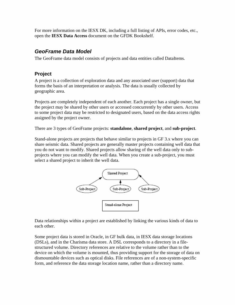
Project A project is a collection of exploration data and any associated user (support) data that forms the basis of an interpretation or analysis. The data is usually collected by geographic area. Projects are completely independent of each another. Each project has a single owner, but the project may be shared by other users or accessed concurrently by other users. Access to some project data may be restricted to designated users, based on the data access rights assigned by the project owner. There are 3 types of GeoFrame projects: standalone, shared project, and sub-project. Stand-alone projects are projects that behave similar to projects in GF 3.x where you can share seismic data. Shared projects are generally master projects containing well data that you do not want to modify. Shared projects allow sharing of the well data only to sub-projects where you can modify the well data. When you create a sub-project, you must select a shared project to inherit the well data.

Data relationships within a project are established by linking the various kinds of data to each other. Some project data is stored in Oracle, in GF bulk data, in IESX data storage locations (DSLs), and in the Charisma data store. A DSL corresponds to a directory in a file-structured volume. Directory references are relative to the volume rather than to the device on which the volume is mounted, thus providing support for the storage of data on dismountable devices such as optical disks. File references are of a non-system-specific form, and reference the data storage location name, rather than a directory name.

GeoFrame data contains storage repositories for project, coordinate and unit information as well as for wells and well related data. Starting with GeoFrame 4.0, the following IESX data types are stored in GeoFrame:

• IESX project name, password, DSL locations • Seismic survey and line information • Complete suite of interpretation data (horizons, faults, contacts, etc.) • Projection, coordinates, units

Data Objects in the GeoFrame Database Most GeoFrame objects are referred to as DataItems (DIs). For a given DataItem, there are properties. Some properties are actual columns in the Oracle tables, while some attributes are themselves DataItems. Finally, other properties of a DataItem are implemented as parameters. Examples of DIs are wellbore, location, and so on. For the wellbore DI, you can retrieve data attributes such as name and UWI. You can also attach a parameter such as Origin to the wellbore.

* Please refer to the SDM Data Item Report and ADI Reference Manual for a

complete explanation on GeoFrame DataItems. The best way to view the SDM Data Item Report is with an internet browser

such as Mozilla. Open a GeoFrame xterm and type the following: >mozilla $GF_PATH/wk_sdm/direport/index.html To access the ADI Reference Manual, click on Application Data Interface

(ADI) Reference Manual in the GFDK Bookshelf.

In the IESX database, an entity is referred to as a data object. Many IESX objects are stored in GeoFrame. Examples of IESX data stored in GeoFrame are:

• 3D and 2D surveys • 2D lines • Surfaces (horizons, faults) • Interpretation (attributes, fault cuts, contacts, fault boundaries) • Grids • Well data (wellsets, well, borehole, markers, logs, deviations surveys, checkshots)

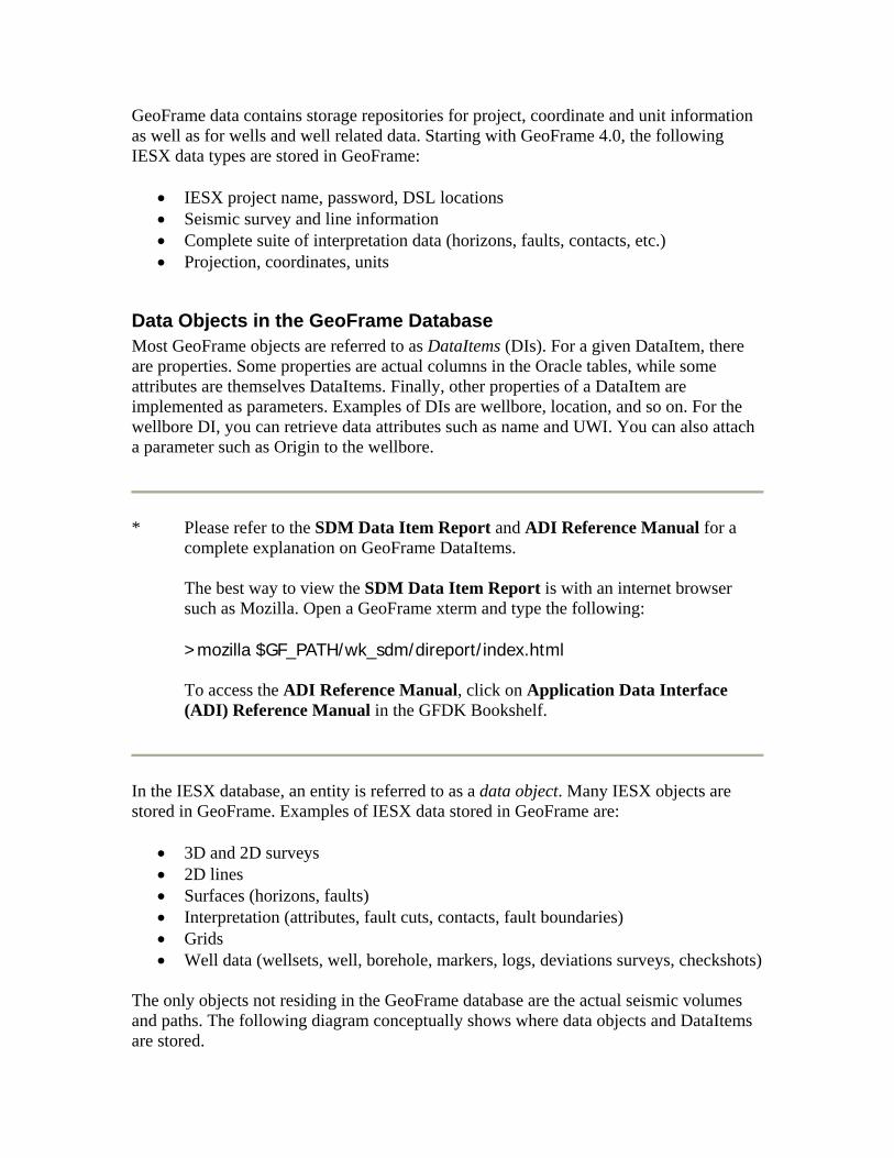
The only objects not residing in the GeoFrame database are the actual seismic volumes and paths. The following diagram conceptually shows where data objects and DataItems are stored.

Exploration object Exploration objects are the primary data objects of a seismic project. Examples of exploration objects are seismic lines (2D) and seismic volumes (3D). Exploration objects are stored in the GeoFrame database. Each exploration object may have several representations. Representations of a seismic line exploration object may include the seismic data itself, the interpretation of the seismic data, and the location of the seismic traces. An exploration object may have multiple instances of a particular kind of representation. For example, a single seismic line may have several instances of seismic data representations (original data, migrated data, stacked data). An exploration object does not actually store its representations; instead, it provides a method of organizing and relating them to each other in the database. An exploration object consists of the data collected (or derived) at a set of observation points, plus data that pertains to the object as a whole. For example, the observations collected at a single point for a seismic line include a seismic trace (or possibly multiple

traces), the interpretation at that trace, and the location of the trace. This common set of observation points defines the spatial relationships among the various representations of an exploration object. The basis of an exploration object is the entity that defines the organization of the observation points. For example, the basis for a seismic line exploration object is the seismic data itself, since it establishes the position of the observation points. It forms the basis for the interpretation and the trace locations. Observation points correspond to surface locations. The set of observation points for an exploration object may be singular (such as a well location), linear (such as a 2D seismic line), or form a 2D rectangular grid (such as a 3D seismic volume). The organization of observation points does not imply that the locations of the points form equivalent geometric figures. 2D seismic lines form a linear array of observations; the points need not be geometrically colinear.

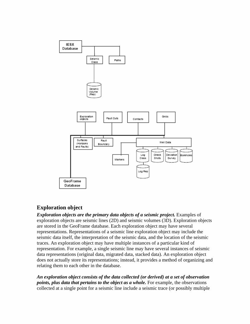
Survey A survey is an area or prospect defined by topographical, geological, or geophysical measurements. A project may contain many surveys as defined by the explorer.

A survey can be classified as a left-handed or right-handed survey. The easiest way to remember is to look down the first inline. If subsequent inlines are to the left, then the survey is left-handed. If subsequent inlines are to the right, then the survey is right-handed. Survey origin is defined to be the location of the minimum i and j (IESX internal coordinate system) and not the actual location where loading starts.

For a given survey, there may be several classes which can represent the different processing methods applied to the survey data. Examples of seismic classes are original, migrated, stacked, etc. For a given survey and a given class, a unique 3D seismic volume is defined. In 2D data, a 2D survey represents a grouping of 2D lines. 2D lines are equivalent in hierarchy to 3D surveys. For a given 2D survey, a given 2D line and a given class, a unique 2D seismic volume is defined.

Well data

[Borehole] data Well data is stored in the GeoFrame database. The data can be retrieved directly using GFDK ADI calls or indirectly using IESX DK calls. IESX DK well data consists of well boreholes, deviation surveys, checkshots, markers and log curve data. IESX DK does not handle well data; it deals with borehole data. In GeoFrame, well data refers to the well head data such as well name, well UWI, status, and surface location, whereas borehole data refers to the rest of the well. Borehole data may include: name, UWI, API, bottom location, hole condition, index, elevation information, flow direction, deviation survey, checkshots, markers, and log data.

Markers Markers are used to indicate the intersection of horizons or surfaces on a well trajectory. Markers have attributes such as name, type, color, source, seismic pick time or depth, index, and associated surface.

Log class Log classes are entities used to differentiate the same type of log data that was acquired at different times using the same logging tool. It is a way of creating versions. Typical log classes are “Sonic” and “Gamma.” Log classes act as containers for log data. The data is stored in log representations in the GeoFrame database.

Log representation Log curves are stored in log representations in the GeoFrame database. Each log representation stores a single log curve. A log representation belongs to both a log class and an exploration object. Each log class–exploration object pair may have many log representations.

Checkshots Checkshots are also known as DVT relationships (D = depth, V = velocity, T = time). The relationship provides the mapping between these three parameters. Each borehole

has a preferred checkshot; that is, all time/depth/velocity relationships are derived from the preferred table.

Deviation survey A deviation survey contains borehole path points delineating the borehole path’s orientation in the earth. Deviation points also represent the departure points of a borehole from vertical. Deviation points are duplets of delta-x versus delta-y, deviation degree versus azimuth, MD versus TVD, and so on.

GeoFrame Interpretation Model The interpretation model is a consistent, user-named collection of interpretation data that can include the following elements:

a. Horizon grids (surfaces) b. Horizon 2D line interpretation c. Fault cuts d. Contact points e. Fault boundaries

In a project, there may be hundreds of interpretations of which only a few are active and of interest to an interpreter. Therefore, instead of scrolling a long list of interpretation, the user may want to select only those of interest to the user and put them into a group called a model. Some of the criteria used to create an interpretation model are:

• Create different interpretation versions (snapshots of interpretation states) • Subdivide a project by area and interpretation to facilitate multiple users working

on the same project • Make interpretation objects within a model read-only, which allows the model to

be shared by multiple users and multiple models within the same project Models are created and edited by the Seismic Interpretation Manager in the Application Manager’s Seismic Catalog. If no model is created, a default time and a default depth model are created. These default models contain all horizons and faults of the corresponding domain. When you open an application in IESX and interpret on a seismic line, those interpretations are added to the selected model in the active domain. If no model is selected, the “Default” model in the active domain is chosen. IESX DK applications and servers behave the same way.

Surface (horizon and fault) Horizons and faults are organizational entities in the GeoFrame database. They do not store any interpretation data.

Horizon Horizons are DataItems in the GeoFrame database and act as containers for horizon attribute data. The GeoFrame database has two types of horizons: seismic and geological. Horizons can be viewed as surfaces with interpreted attributes such as Time, Amplitude, Snap, and so on. Calculated attributes can also be generated for a horizon. Only seismic horizons are returned from IESX DK interfaces. See the GeoFrame DI Report for more information on horizon surfaces.

Grid data Grid data are stored in GeoFrame and consist of a binset which controls the orientation and extent. Grid data has a value (may be null) for every node in a regular spaced framework. Starting with GF4.0.4, binsets can be skewed. A new member (skew_angle) was added to the htp_grid_data_geom_s to denote the skew angle if the binset is skewed. Hence, a skew angle of 0 or 90 degrees means that the binset is not skewed. There are two types of grid supported by IESX DK: interpreted vs. computed grids. Interpreted grids are grid data generated by interpretation applications and are generally limited by the binset corresponding to a seismic survey extent. Thus, interpreted grids are tied to seismic surveys. All horizon attributes data are now stored in GeoFrame as interpreted grids and they are accessed via the htp_hor_xxx interfaces. Interpreted grids are covered in the next section. Computed grids are grids resulting from arithmetic operations or any other grid operations (i.e., isochron, etc) or simply any 2 dimension arrays of grid data. Computed grids can also be skewed. Computed grids are access via htp_grid_xxx functions. Interpreted grids always belong to an interpretation model while computed grids are model independent. Fault surfaces generated by tessellation or by gridding are stored in GeoFrame as computed grids and not as interpreted grids. The GeoFrame grid system has adopted orientation 2 (LHP - left hand plane) as the only recognized orientation, meaning all grid data are returned and written via IESX DK in the

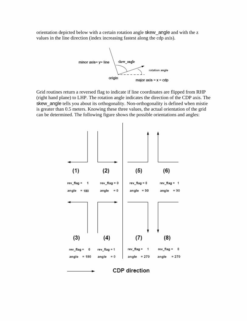
orientation depicted below with a certain rotation angle skew_angle and with the z values in the line direction (index increasing fastest along the cdp axis).

Grid routines return a reversed flag to indicate if line coordinates are flipped from RHP (right hand plane) to LHP. The rotation angle indicates the direction of the CDP axis. The skew_angle tells you about its orthogonality. Non-orthogonality is defined when mistie is greater than 0.5 meters. Knowing these three values, the actual orientation of the grid can be determined. The following figure shows the possible orientations and angles:

Horizon attribute Starting in GeoFrame 4.0, all 3D horizon attributes are stored in the GeoFrame database as interpreted grids, and they are associated with a seismic binset. 2D horizon attributes are stored in GeoFrame as line data. 2D and 3D horizon attribute data are accessed via htp_hor_xxx and htp hor_attr routines. Each attribute [grid] has a property code and unit which are stored in the GeoFrame property catalog and viewable via sqlplus. Property unit can be unitless.

Horizon attribute name There were changes in the naming convention of horizon attributes in GeoFrame 4.0. Some attributes do not require any name (for example, Time attribute), some require a seismic class name (for example, Acoustic Amplitude) and others optionally can allow a user-defined name. You can create an attribute with any property code and unit. However, attributes created this way may not be recognized by IESX applications. IESX applications recognize only a sub-set of property codes from over 3,400 property codes known to GeoFrame. The complete list of IESX recognizable attributes is listed in the appendix of the IESX Data Access document on the GFDK Bookshelf. The following horizon attributes do not require attribute names and are generated by IESX Seismic Interpretation, ASAP, and AutoPix applications:

• Time • Snap_Criteria • Interpretation_Origin • Pick_Quality

Attributes not requiring attribute names and generated by MisTie applications are:

• Tie_Point_Total_Time_Correction • Tie_Point_Phase_Shift • Mis_Tie_Phase_Correction • Mis_Tie_Static_Time_Correction • Mis_Tie_Variable_Time_Correction • Tie_Point_Time_Quality

Only Acoustic_Amplitude requires that the attribute name be the seismic class name. Acoustic_Amplitude generated from Seismic Interpretation has the attribute name built as “class_name#amp” while the acoustic amplitude generated by AutoPix has the attribute name as “class_name#amp2”. The complete attribute name has the following format: property code, space, ampersand as delimiter, space, attribute name as in “property_code & attribute_name”. The attribute names can be actual seismic class name, blank, or user-

defined names. Examples of attribute names where migrated is a seismic class name are listed below:

• Time • Acoustic_Amplitude & migrated • Acoustic_Amplitude & migrated_#amp2 • Time & migrated_#time1

To get the complete list of the GeoFrame property code, run sqlplus on the baseline account or on your project and query for property_cat and property_catr respectively. To get property code from a catalog baseline, you will need Administrator privilege. The list of property codes obtained from your project and from the catalog baseline is identical. In order to get property codes from your project, your project must have interpretation or you must have caused the loading of the property codes into your project (for example, launch horizon dialog).

* If you need help with the sqlplus queries, please refer to Chapter 3 in the IESX

Data Access document on the GFDK Bookshelf.

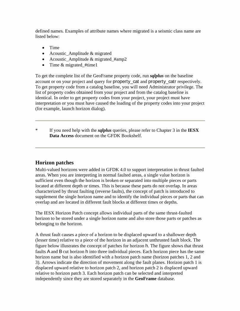
Horizon patches Multi-valued horizons were added in GFDK 4.0 to support interpretation in thrust faulted areas. When you are interpreting in normal faulted areas, a single value horizon is sufficient even though the horizon is broken or separated into multiple pieces or parts located at different depth or times. This is because these parts do not overlap. In areas characterized by thrust faulting (reverse faults), the concept of patch is introduced to supplement the single horizon name and to identify the individual pieces or parts that can overlap and are located in different fault blocks at different times or depths. The IESX Horizon Patch concept allows individual parts of the same thrust-faulted horizon to be stored under a single horizon name and also store those parts or patches as belonging to the horizon. A thrust fault causes a piece of a horizon to be displaced upward to a shallower depth (lesser time) relative to a piece of the horizon in an adjacent unthrusted fault block. The figure below illustrates the concept of patches for horizon h. The figure shows that thrust faults A and B cut horizon h into three individual pieces. Each horizon piece has the same horizon name but is also identified with a horizon patch name (horizon patches 1, 2 and 3). Arrows indicate the direction of movement along the fault planes. Horizon patch 1 is displaced upward relative to horizon patch 2, and horizon patch 2 is displaced upward relative to horizon patch 3. Each horizon patch can be selected and interpreted independently since they are stored separately in the GeoFrame database.

When you add a horizon to an interpretation model, a default horizon patch is created for the new horizon. Patch names are named sequentially as 001, 002 by default unless overridden by a user defined patch name. GeoFrame provides the capability to re-order patches in the Horizon Patches Data Manager in the Data Management Catalog.

Fault Faults are DataItems in the GeoFrame database and act as containers for fault interpretation data. The fault record is stored in the GeoFrame database. Starting in IESX 4.0, fault surfaces are generated in IESX Seismic Interpretation applications and stored in the GeoFrame database as grids regardless of whether those surfaces were generated by tesselation or by gridding. See the GeoFrame DI Report for more information on fault surfaces.

Fault cut A fault cut is a polyline defined by i, j, z in an exploration object in the GeoFrame database, where i = crossline j = inline z = time or depth A fault cut is a 2D projection of a single fault. Typically, a fault contains many fault cuts. A fault cut must be contained by a single exploration object.

Interpretation contact An interpretation contact is a point defined by i, j, z in an exploration object in the GeoFrame database. Interpretation contacts are usually used to mark a point at which two objects touch. A contact may be one of several types:

• Horizon-Horizon • Horizon-Fault • Fault-Fault • Pinchout • Term (termination) • Unused

Fault boundary A fault boundary, like a fault cut, is a polyline defined by the real-world x, y, z coordinates and stored in the GeoFrame project. Because fault boundaries are defined by real-world coordinates, they may span exploration objects. A fault boundary is associated with a given horizon and fault. Contacts are not longer associated with fault boundaries.

IESX Data Model In the IESX database, a single entity is referred to as a data object. (In the GeoFrame database, an entity is referred to as a DataItem.) Examples of IESX data objects are seismic volumes and paths. Some objects, such as seismic volumes, are permanent and are stored in the disk files of the database. Other objects, such as paths, may be temporary or permanent and are stored in memory while the database is accessed. Objects may either be tangible (such as a seismic volume) or abstract (such as an object connection referred to as token). All data objects belong to a category which can be thought of as an aggregation of objects that have the same properties or behavior. Examples of categories are seismic classes and paths.

IESX Local coordinate system The observation points for an exploration object define a local coordinate system (LCS) for that object. A local coordinate system corresponds to the map view of the exploration object’s observation points. There is no mapping between LCSs for different exploration objects. To define spatial relationships among exploration objects, the actual location data must be used. A local coordinate system is either a 1D or 2D coordinate system,

depending on the arrangement of the observation points. A 2D seismic line has a 1D LCS, and a 3D seismic volume has a 2D LCS. The degree of a local coordinate system specifies whether the LCS has one or two dimensions. A local coordinate system does not define a vertical dimension because the units of vertical distance vary among different exploration objects or representations of the same object. A local coordinate system is normalized to the observation points of the object—the distance between adjacent observation points is 1. A local coordinate system is non-discrete, and points intermediate to the observation points may be specified. The interpretation of these non-integral coordinates depends on the type of access made to the database. Typically, it implies an interpolation of the data. A local coordinate system is considered to be infinite. The extent of the finite sub-region of this infinite space where data is actually defined is maintained by the database. Typically, specified coordinates lie within or near this extent of defined data. The origin of the LCS no longer corresponds to the first observation point for which data is loaded. It is defined to be the minimum LCS values. No assumption should be made that LCS coordinates are positive. The values of LCS can be positive, negative, and 0. However, the LCS increments are always positive. A linear mapping is defined between user-defined coordinates, such as line numbers and CDP numbers, and an LCS. No assumption should be made that minimum LCS correspond to minimum RCS (line and CDP numbers). In many instances, as LCS values are increasing, RCS values may be decreasing. The best way is to look at the transformation tables for the corresponding axis - inline and CDP transformation tables for 3D surveys and SP and CDP tables for 2D lines. When data for an observation point (such as a seismic trace) is loaded, this mapping is used to compute the local coordinate of the trace. In cases where the physical organization of data is the same as the local coordinate system, the local coordinate is used to determine where the data is stored in the physical structure. This allows data to be loaded into a representation of an exploration object in an arbitrary order.

Seismic class Seismic classes in the IESX database are entities used to organize seismic data into various groups. A seismic class does not contain seismic data; the data is stored in the IESX database in seismic representations. Examples of seismic classes might be “Original Data” and “Filtered Data.”

Seismic representation Seismic representations are the entities in the IESX database that contain the seismic data. A seismic representation belongs to both a seismic class and an exploration object. There can only be one seismic representation for each seismic class and exploration object pair. The seismic representation contains the line/volume header for the seismic data. This header is an expanded version of the SEG-Y line header.

Trace header Each trace contains a header, which is a superset of the SEG-Y trace header, and sample data. Each trace contains the same number of samples. This number is set when the seismic representation is created. To represent nonrectangular surveys (2D exploration objects) with the rectangular seismic representation, each trace has an existence flag in its header. This flag can take on one of three possible values:

• DB_LIVE_TRACE indicates a normal trace • DB_DEAD_TRACE indicates a trace in which all samples are zero • DB_NULL_TRACE indicates a trace that does not exist in the seismic survey,

although it is in the rectangular area of the seismic representation DB_NULL_TRACE traces exist because of restrictions in the storage mechanism, but are marked to allow applications to treat them as needed.

Storage of seismic traces (bricks) Seismic traces are stored in a volume as bricks to allow quick access of spatially oriented grid data. The data set is a gridded cube of dimensions p, q, r. Brick Access Tools (BAT) break this gridded cube into bricks of the requested p, q, and r size. BAT is based on the principle of local reference; thus, for any given p, q, r coordinate, BAT issues one lower-level IO call to retrieve all the data for the brick in which the specified p, q, r resides. The seismic traces (bricks) are stored in regular flat-files. Brick offsets that point to the starting location of the brick (with some additional bookkeeping information) are maintained in an indexed file using the indexed IO capability of the lower-level IO facility. Optionally, a logical BAT file can be split into several physical files, where each file could possibly exist on a different physical disk volume. The physical spread across volumes is transparent to BAT users. On each brick write, BAT checks for the violation of the selected criterion. On failure, it acquires a new DSL (volume) and continues writing on the new volume. Currently, BAT can handle 255 distinct physical files (therefore, potentially 255 distinct volumes, although the current DB tools that work with it support up to 64 DSLs).

A bat brick varies in size from 8K to 256K. Within a volume, the brick size is constant. BAT can reuse bricks that have been marked as deleted.

Path A path is used to specify the region of an exploration object that is to be read or written by database routines. It is also used as a mechanism for communication between applications and other toolkit routines. For example, a path could be used to specify the portions of a seismic volume to be displayed by a seismic display routine. A path is specified by an exploration object, a spatial region, and a vertical range. The spatial region is composed of a set of figures. The figures may be areal (usually a rectangle), linear (polylines), or singular (points). The local coordinate system for the exploration object is used to specify the vertices of the figures. The spatial region defines a set of observation points. This set of points is made up of the points interior to areal figures, along linear figures, and near point figures. The vertical range for a path is a pair of values specified in units of time or depth. The range may be specified relative to a zero time or depth (from a datum), relative to a time or depth data (from the time of first sample TFS), or relative to a horizon. A sub-range of the path may be established by specifying a range within the set of observation points, a decimation within that range, and a sub-range of the vertical range. When data is read or written, the data is within the sub-range of this path. Initially, all paths are of the type DB_PATH_VIRTUAL. Only when a constructed path is saved does it become DB_PATH_PERMANENT. A path of type DB_PATH_VIRTUAL exists only within the context of the current execution, whereas a path of the type DB_PATH_PERMANENT is saved with a name for future reference. The paths of type DB_PATH_TEMP exist between two sessions, to restore the saved context. They do not exist (on the disk) once the session is restored. The concept of paths is extended in a 2D or 3D survey to encompass traverse through multiple surveys and exploration objects. These are commonly known as trips. The current implementation of trips limits the “trip type” to DB_TYPE_POLYLINE and DB_TYPE_LIST. All other conditions that apply to paths are valid with regard to the type of persistence, ranges, extents, and so on.

IESX DK Model The IESX DK allows users to develop applications that appear as integrated components of IESX or as stand-alone applications loosely tied to the IESX database. The IESX DK applications are the clients in a client–server model. Each client application has a server. The client and server use sockets and shared memory to communicate with each other.

The IESX DK server can be either IESX User Applications or one of the stand-alone servers thtp or batch_thtp. IESX User Applications provide different means for launching the integrated IESX DK application. Communication between the IESX server and IESX DK applications are done via sockets and shared memory. Small packets of information are communicated via socket, whereas large packets of information (for example, seismic traces) are communicated via the shared memory. Each IESX DK client–server pair has one socket and one shared memory. Because of the shared memory, IESX DK servers and clients must be run in the same memory space (on the same CPU). The IESX DK server sets up the socket and the shared memory during initialization and sends this information to the client application. Setup of the socket and the shared memory in the client application is done in the htp_init_comm interface call. The IESX DK server is always listening in a predetermined socket for requests from the IESX DK client application. Termination of the socket and release of the shared memory is done in the htp_term_comm call. In general, when an IESX DK application wants information, it makes an htp_xxx API call, which sends the data type of the request via the socket. The server receives the requested data type and calls the appropriate htp routines to service the request. Additional information (name and data) may be sent by the IESX DK applications to the server in the shared memory, to complete the processing. For ease of use and maintenance, all these interprocessing communication calls are embedded in the htp_xxx API calls. htp data is generally grouped into a structure to ease additions to the members of the structure without modifying the IESX DK API sequence call from IESX applications. Whereas the IESX DB uses tokens for handling data objects, IESX DK uses the name of the data object. This makes programming and support easier, because the IESX DB tokens have no context outside IESX. A survey, input class, and output class must be defined before any seismic or interpretation attribute objects (such as horizon attributes, fault cuts, contacts, and the preferred fault boundary set) are accessed in either read or write mode. You can generate a dummy output class if your IESX DK applications are for read-only. Well data does not require the selection of survey or seismic classes for access. IESX DK maintains internally a list of the following defined objects:

• Seismic path points • Horizon attribute in and out path points • Fault path points • Contact path points • List of defined horizons, patches, and attribute names

• List of defined fault names • Domain selection • Model selection

After an IESX DK executable file is selected, the IESX DK server starts the IESX DK application as a new process. Both the IESX server process and the IESX DK application process go into an initialization phase wherein they establish a communication channel between themselves. The communication is based on TCP-BSD sockets and shared memory. The next stage is for the two participants to handshake and exchange any initial data. For example, the user procedure can obtain the list of horizon attributes and faults, the selected path, and so on. At this point the user procedure can reset any of these selections. The user procedure may also define new traversal paths along which the data is to be fetched. This option allows the user process to traverse the data randomly. The paths can be distinct for different accesses; for example, the seismic access path and the interpretation access path could be different from each other. 1. In the initial processing phase, the application does the following operations:

a. Defines a domain. b. Defines an interpretation model. This step can override the previous step in

selecting a domain. It is much more efficient to select a model and a domain at the same time than selecting a domain and an interpretation model separately.

c. Defines the I/O access patterns for each data type to be accessed (that is, each seismic, interpretation, fault, and contact has its own input and output paths). This occurs only once, at the beginning.

d. Obtains the access path(s) for the survey for each of the data types. e. Obtains the list of selected horizons, patches, and attributes. f. Creates horizons, patches, and attributes if needed. g. Defines a new set of horizons, patches, and attributes. h. Obtains the set of faults selected for fault data access. i. Defines a new set of faults (or creates it if it does not exist). j. Obtains the line header information pertaining to the current survey.

2. Operations c-j can be repeated after the initialization phase. These operations allow the user procedure(s) to select and define data access based on earlier accesses. 3. After applications are past the initial handshake data exchange, they drop into a processing loop where they can do the following operations, assuming that the IESX DK application has a selected survey, and input and output class, horizon attributes, faults, and contact data:

• Get the seismic trace data.

• Put the seismic trace data. • Get horizon-patch-attribute information (either in trace mode, path mode, or

rectangular mode). • Put horizon-patch-attribute information (either in trace mode, path mode, or

rectangular mode). • Get fault information. • Put fault information. • Get contact information. • Put contact information.

Compiling and Linking IESX DK Applications There are two types of IESX DK programs: GeoFrame non-compliant and GeoFrame compliant. If you do not need to access the ADI layer in the GFDK, then you will likely be building GeoFrame non-compliant IESX DK programs. However, if you do need direct access to the ADI, then you should consider building GeoFrame compliant IESX DK programs or GFDK programs (as described in the GFDK Integration section). Each of the two types of IESX DK programs has its own way of being compiled and linked, so depending on the application, you will need to choose how you want to build your IESX DK program. Before compiling and linking your IESX DK applications, it is strongly advised to set up your work area and copy necessary files from the GeoFrame baseline to your work area. You will need to set up a search path between your user area and the GeoFrame baseline using the gfpath command, and you will need to add the ies_htp set. Then, you should copy all of the files in the GeoFrame baseline ies_htp set to your user area ies_htp set. To accomplish these steps, you can perform the following: 1. Launch a GeoFrame xterm. 2. If you have already created a user area, type the following in the GeoFrame xterm: >gfpath –add –set ies_htp If you have not created a user area, type the following in the xterm: >gfpath –create <user_directory (can be ‘.’)> <directory_spec_of_baseline> -add -set ies_htp 3. Copy all of the files from the GeoFrame baseline ies_htp set to your user area ies_htp set. >cp $GF_PATH/ies_htp/* <user_directory>/ies_htp/

GeoFrame non-compliant IESX DK When direct access to the ADI layer is not needed, you are likely to build GeoFrame non-complaint IESX DK programs. This flavor of IESX DK program is typically compiled and linked using “make –f”.

Template The IESX DK provides a template C source code file as well as a template makefile to give you a starting point for creating your own IESX DK programs. It is strongly recommended to use these templates when building your own IESX DK programs. Both files are found in the ies_htp set. Depending on your platform, you need to select the correct makefile. If you are using a Linux system, then you should use make_template_linux.dat. Otherwise, if you are on a UNIX system (Sun/Solaris), then you should use make_template.dat. There is only one template C source code file (dk_template.c). It can be built with either makefile depending on the platform you are on. The template program is comparable to a “Hello world” program. The IESX DK template program initializes communication to GeoFrame, prints out “After init comm” to the xterm, terminates the process, and ends communication with GeoFrame.

Compiling the template From a GeoFrame xterm in your work area, type the following: Linux >make –f ies_htp/make_template_linux.dat Sun/Solaris >make –f ies_htp/make_template.dat If successful, you should now have a binary called dk_template in your work area’s bin directory.

Adapting the template To make your own GeoFrame non-compliant IESX DK programs, you should start out by making a copy of the template makefile for your platform and the template C source code file. For instance, copy the make_template.dat to make_my_dk.dat and the dk_template.c file to my_dk.c. In a text editor, open the make_my_dk.dat file and change the PRG_NAME variable to my_dk. If you have more than one source file, make the necessary changes to the

makefile to compile and link the source files to generate one executable. Basically, modify the OBJECTS variable and add the additional source files to the bottom of the makefile. To write your own IESX DK code, open the source file (my_dk.c) with a text editor and add your code directly above the “all_done” label. Depending on the types of data objects you are planning to use in your application, you may need to modify the boolean flags set in the common_in structure. At the end of this chapter, we provide a few IESX DK example programs.

GeoFrame compliant IESX DK When compiling and linking GeoFrame compliant IESX DK programs, you must use gbuild and launch your programs using the IESX DK servers.

Template For GeoFrame compliant IESX DK programs there are three important template files: a source code file, a .lnk_def file, and a .sql file. Again, it is recommended to make copies of these files and adapt them as necessary. The template files are found in the ies_htp set. The gf_template.c file is the template source code file for GeoFrame compliant IESX DK programs. The gf_template.lnk_def file should be used regardless of platform to link GeoFrame compliant IESX DK programs. The gf_template.sql file is the template sql file. You will use the sql file to register your IESX DK program with GeoFrame.

Compiling the template From a GeoFrame xterm in your work area, type the following: >gbuild ies_htp/gf_template If successful, you should now have a binary called gf_template in your work area’s bin directory.

Adapting the template To start making your own GeoFrame compliant IESX DK programs, you should make copies of the three template files.

In the .lnk_def file, you will need to change the gf_template.o to the .o files for your source files. In the source file, you will add your code in the RunApplication function after the comment /* add your codes here */. In the .sql file, you should change all instances of gf_template with the name of your executable. Please look at the end of this chapter to find IESX DK example programs.

Launching IESX DK Applications There are 3 main ways to launch IESX DK applications: batch_thtp, IESX User Applications, thtp. GeoFrame non-compliant IESX DK programs can be launched with any of the three methods to launch an IESX DK program, while GeoFrame compliant IESX DK programs should only be launched with IESX User Applications. Before delving into the 3 methods of launching an IESX DK application, we must describe how to register an IESX DK application if you plan to use IESX User Applications or thtp. Also, we show you how to check the version number of the DK application in the case that you try to upgrade your DK applications from an older GeoFrame release to a newer one. Whenever you upgrade GeoFrame, you must rebuild your DK applications to ensure compatibility with GeoFrame.

Registering an IESX DK application To register an IESX DK application with the IESX DK server for use in IESX User Applications or in thtp, you must add the executable name and the path to the executable in a file defined in the IESX_USER_APPL environment variable. The file can reside in any directory you specify, but you must make sure to set the IESX_USER_APPL environment variable to point to it, otherwise your IESX DK applications will not be listed in the user applications list. It is recommended to name the file iesx_user_appl.dat, but you can choose any name you like. To set up the IESX_USER_APPL environment variable, open a GeoFrame xterm, and type the following: >setenv IESX_USER_APPL /home/xxx/xxx/iesx_user_appl.dat Each record of the iesx_user_appl.dat file contains the name of the executable and the path of that executable in the system. For example: htp_test_attr /home/ie/gftc/law/gfwork/bin/htp_test_attr

Also, each record in the iesx_user_appl.dat file should start at the beginning of a new line.

Checking the version number of the application Generally, each major IESX DK release is distributed with a change in the IESX DK version number in htp_version.h. The IESX DK server checks for the version number in all IESX DK applications invoked from the IESX User Applications or from thtp. If it finds the correct version number in the executable, that IESX DK application is added to the list of applications in the application list box, and thus, can be selectable. IESX DK version is a string of the word version followed by the release number, which is encoded in the compile run and checked at run time. The IESX DK version number for GeoFrame 4.4 is 4.1.0. To check what version of IESX DK your application is linked with, type the following at a GeoFrame xterm: >strings <IESX_DK_application_name> | grep VERSION For example: >strings bin/dk_template | grep VERSION The system returns: VERSION 4.1.0 This means that dk_template was compiled with IESX DK version 4.1.0. This forces all IESX DK applications to be recompiled and relinked when a new IESX DK kit is received and to ensure that all IESX DK applications are compatible with the current IESX DK deliverables and IESX database. IESX DK applications will not show up in the IESX DK applications list if the IESX DK versions of the server (thtp, IESX User Applications) and the IESX DK applications are not compatible meaning IESX DK servers and IESX DK applications were compiled and linked against IESX DK libraries of different version numbers. For example:

• You invoke thtp or IESX User Applications that is not linked with the correct IESX DK version number. Consequently, the list of DK applications is blank.

• This often occurs during the development of a newer IESX DK library. For example, your default system is running IESX DK version 3.7.0, but you are developing for IESX DK 4.0.4. In order to sync the IESX DK server and your DK applications, you must invoke thtp from the proper baseline (GFDK 4.0). In this case, this server does not see IESX DK applications linked with version 4.0.4.

• You have not recompiled and relinked your IESX DK applications with the latest IESX DK libraries. For example, you have launched IESX DK server from GFDK 4.0 while your DK applications were compiled and linked under GFDK 3.x.

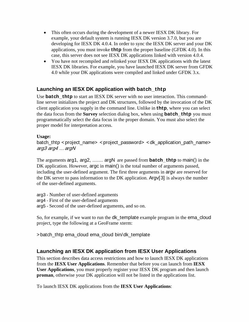
Launching an IESX DK application with batch_thtp Use batch_thtp to start an IESX DK server with no user interaction. This command-line server initializes the project and DK structures, followed by the invocation of the DK client application you supply in the command line. Unlike in thtp, where you can select the data focus from the Survey selection dialog box, when using batch_thtp you must programmatically select the data focus in the proper domain. You must also select the proper model for interpretation access. Usage: batch_thtp <project_name> <project_password> <dk_application_path_name> arg3 arg4 … argN The arguments arg1, arg2, ....... argN are passed from batch_thtp to main() in the DK application. However, argc in main() is the total number of arguments passed, including the user-defined argument. The first three arguments in argv are reserved for the DK server to pass information to the DK application. Argv[3] is always the number of the user-defined arguments. arg3 - Number of user-defined arguments arg4 - First of the user-defined arguments arg5 - Second of the user-defined arguments, and so on. So, for example, if we want to run the dk_template example program in the ema_cloud project, type the following at a GeoFrame xterm: >batch_thtp ema_cloud ema_cloud bin/dk_template

Launching an IESX DK application from IESX User Applications This section describes data access restrictions and how to launch IESX DK applications from the IESX User Applications. Remember that before you can launch from IESX User Applications, you must properly register your IESX DK program and then launch proman, otherwise your DK application will not be listed in the applications list. To launch IESX DK applications from the IESX User Applications:

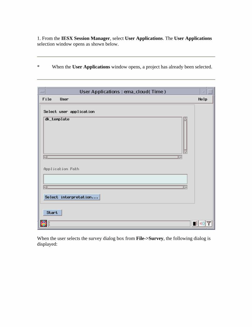
1. From the IESX Session Manager, select User Applications. The User Applications selection window opens as shown below.

* When the User Applications window opens, a project has already been selected.

When the user selects the survey dialog box from File->Survey, the following dialog is displayed:

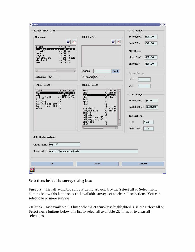
Selections inside the survey dialog box: Surveys – List all available surveys in the project. Use the Select all or Select none buttons below this list to select all available surveys or to clear all selections. You can select one or more surveys. 2D lines – List available 2D lines when a 2D survey is highlighted. Use the Select all or Select none buttons below this list to select all available 2D lines or to clear all selections.

Input class – List classes when a survey (2D or 3D) is highlighted. For a single 3D survey or a single 2D line, all classes belonging to the input survey or line are listed. For multiple surveys or multiple line selections, only the seismic classes that are common to the selected surveys are listed. Output class – Select an output class for the selected operation. The output class is labeled as attribute volume. Line, CDP, and Trace ranges:

• For multiple survey and/or multiple line selection, line range and CDP range text boxes are dimmed (inaccessible).

• If a single 3D survey is selected, both the line and CDP range may be specified. • If a single 2D line is selected, only the trace range may be specified.

* The Start and End of the Line range, CDP range, and Trace range are shown

above each text box. To restore the full range, simply click on the input class for the type of data selected.

Time Range

• Sub-volume selection Decimation:

• Line decimation applies to 3D data only. (It is dimmed for 2D data.) • The CDP/trace decimation entry decimates 3D data by the CDP increment, and

2D data by the trace increment. Attribute volume: Class Name – Display the name of the selected Output volume. You can change the name. Description – Enter a description of the selected Output volume. Any combination of characters (including spaces) can be used, up to the end of the text box. Command Buttons The three command buttons at the bottom of the Survey dialog box are Path, OK, and Cancel:

Path – Specify a previously defined traverse, rectangular, or polygonal path (area) for processing. This option is applicable only to 3D data. Selection of this button opens the Path selection dialog box in which to select or enter the path. Note: Selection of a polygonal path dims the Line, CDP, and Trace ranges in the Survey dialog box; that is, they are inactive. OK – Save the survey data selections and close the dialog box. If the output class does not exist, a new output class is created. Cancel – Disregard the survey data selections and close the dialog box. After selecting a survey, you can now change the domain, otherwise the default is Time. 2. In the User Applications dialog box, select User->Domain and choose either Depth or Time. 3. Click on one application.

* Note: You can select only one application at a time.

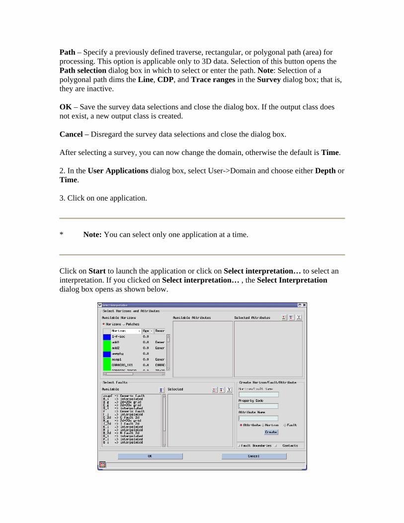
Click on Start to launch the application or click on Select interpretation… to select an interpretation. If you clicked on Select interpretation… , the Select Interpretation dialog box opens as shown below.

• Select horizon attributes, faults, all contacts, and/or fault boundaries to be sent to

user-written executables. • You can change their order by moving them up or down or you delete them from

the list. • You can also create a new horizon, horizon attribute, or fault by entering a new

name in the corresponding text box and pressing the Create button. • Click on OK to accept the selected interpretation and close the dialog box, or

click Cancel to discard the changes.

* Note: Alternatively, you can define horizons, horizon attributes, and/or faults

programmatically.

If you clicked Start, then a progress box is displayed indicating the progress of the selected operation. 4. Click on File->Exit to close the User Applications dialog box or select another application and click Start.

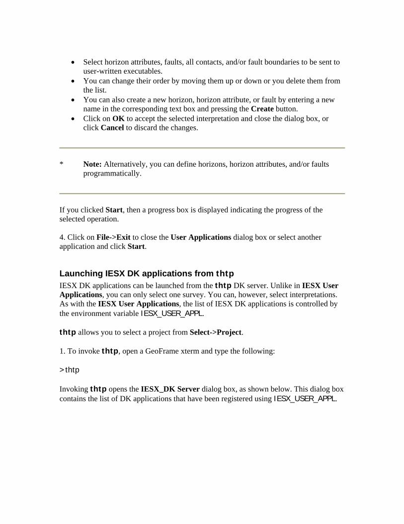
Launching IESX DK applications from thtp IESX DK applications can be launched from the thtp DK server. Unlike in IESX User Applications, you can only select one survey. You can, however, select interpretations. As with the IESX User Applications, the list of IESX DK applications is controlled by the environment variable IESX_USER_APPL. thtp allows you to select a project from Select->Project. 1. To invoke thtp, open a GeoFrame xterm and type the following: >thtp Invoking thtp opens the IESX_DK Server dialog box, as shown below. This dialog box contains the list of DK applications that have been registered using IESX_USER_APPL.

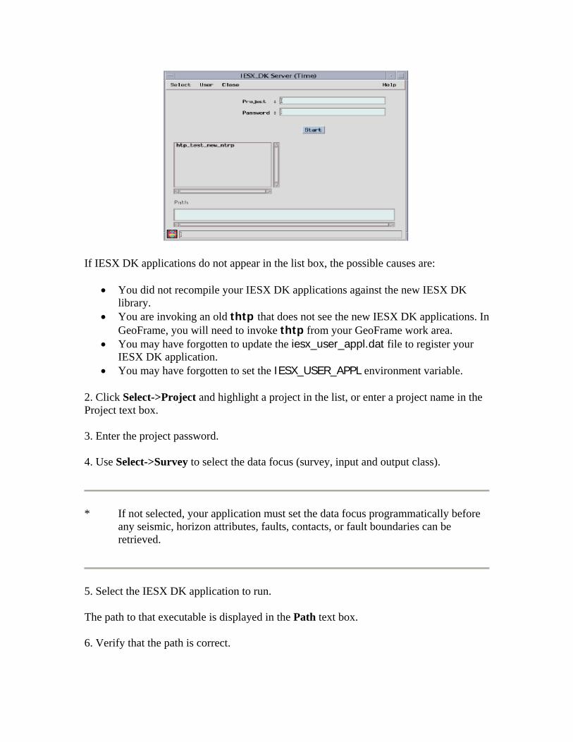
If IESX DK applications do not appear in the list box, the possible causes are:

• You did not recompile your IESX DK applications against the new IESX DK library.

• You are invoking an old thtp that does not see the new IESX DK applications. In GeoFrame, you will need to invoke thtp from your GeoFrame work area.

• You may have forgotten to update the iesx_user_appl.dat file to register your IESX DK application.

• You may have forgotten to set the IESX_USER_APPL environment variable. 2. Click Select->Project and highlight a project in the list, or enter a project name in the Project text box. 3. Enter the project password. 4. Use Select->Survey to select the data focus (survey, input and output class).

* If not selected, your application must set the data focus programmatically before

any seismic, horizon attributes, faults, contacts, or fault boundaries can be retrieved.

5. Select the IESX DK application to run. The path to that executable is displayed in the Path text box. 6. Verify that the path is correct.

If not, modify the path in the iesx_user_appl.dat file. 7. If the domain is not set, it is default to Time. 8. Press Start. thtp sets up the socket, initializes the shared memory, and initializes all thtp structures according to your selection. The Close menu allows you to exit or quit. The exit option allows thtp to remember the project name for subsequent invocations of thtp.

IESX DK Example Programs Since code is dynamic in nature, we try not copy and paste our examples in this document. Instead, we provide the location and file names of the example programs and describe the programs’ functionality in this document. All 6 IESX DK programs are intended to be run with batch_thtp. Before building and running the IESX DK examples, make sure that you have performed the steps in the Compiling and Linking IESX DK Applications section. Namely, make sure that you have added the ies_htp set to your GeoFrame work area by using the gfpath command, and ensure that you have copied all of the contents in baseline’s ies_htp directory into your working area’s ies_htp directory. You must have gcc for Linux or cc for Solaris to build these examples! Before issuing the make command when building these example programs, you must issue a gfpath command so that the proper libraries are linked. NOTE: the gfpath command only needs to be issued once if you plan to build several examples as long as you use the same GeoFrame xterm. For example: >gfpath >make –f ies_htp/make_grid_example.dat >make –f ies_htp/make_horizon_example.dat Before running any of the IESX DK programs, you should make sure to set the TWO_TASK environment variable to the correct database server for your project. The database server can be found in the Project Manager’s Login tab. >setenv TWO_TASK database_server_name

IESX DK Example 1: Create a 3D survey populated with trace data The htp_3dsurvey_example program allows the user to read trace data from a 3d survey in a project, or create a 3d survey in the project and write trace data to it. The program prompts the user for various inputs throughout the execution of the program. When prompted, the user should enter information in the GeoFrame xterm.

How to build htp_3dsurvey_example In your GeoFrame work area’s ies_htp set, you should have copied the following files needed to build htp_3dsurvey_example: htp_3dsurvey_example.c – Main C source file make_3dsurvey_example.dat – Solaris makefile make_3dsurvey_example_linux.dat – Linux makefile If you do not have these files, copy them from the GeoFrame baseline now ( >cp $GF_PATH/ies_htp/*3dsurvey* ies_htp/ ). For Linux, type the following at the GeoFrame xterm in your GeoFrame work area: >make –f ies_htp/make_3dsurvey_example_linux.dat For Solaris, type the following at the GeoFrame xterm in your GeoFrame work area: >make –f ies_htp/make_3dsurvey_example.dat Upon a successful build, you will see htp_3dsurvey_example in your bin directory. If there are syntax errors in compilation, fix them, and try to build again.

How to run htp_3dsurvey_example To run the htp_3dsurvey_example program, type the following in your GeoFrame xterm: >batch_thtp proj_name proj_passwd bin/htp_3dsurvey_example When prompted, enter information in the GeoFrame xterm.

Viewing htp_3dsurvey_example Results If you selected the “read” options, then you will have seen your results in the GeoFrame xterm. However, if you chose the “write” options, you should use Basemap and/or Seis3DV to see your results.

To view your created 3d survey, open Basemap, hit Post->Surveys…, select your survey, and hit Apply or OK. To view your trace data, open Seis3DV, hit Display->Seismic line…, select the proper domain, survey, class, and inline/crossline, and hit OK. To check the trace values, zoom in on an area of interest and hit Shift+MB1.

IESX DK Example 2: Create a 2D line in a 2D survey with shot points The htp_2dsurvey_example program allows the user to read trace data from the 2d surveys and lines in a project, or create a 2d survey and line in the project and write trace data to it. The program prompts the user for various inputs throughout the execution of the program. When prompted, the user should enter information in the GeoFrame xterm.

How to build htp_2dsurvey_example In your GeoFrame work area’s ies_htp set, you should have copied the following files needed to build htp_2dsurvey_example: htp_2dsurvey_example.c – Main C source file make_2dsurvey_example.dat – Solaris makefile make_2dsurvey_example_linux.dat – Linux makefile If you do not have these files, copy them from the GeoFrame baseline now ( >cp $GF_PATH/ies_htp/*2dsurvey* ies_htp/ ). For Linux, type the following at the GeoFrame xterm in your GeoFrame work area: >make –f ies_htp/make_2dsurvey_example_linux.dat For Solaris, type the following at the GeoFrame xterm in your GeoFrame work area: >make –f ies_htp/make_2dsurvey_example.dat Upon a successful build, you will see htp_2dsurvey_example in your bin directory. If there are syntax errors in compilation, fix them, and try to build again.

How to run htp_2dsurvey_example To run the htp_2dsurvey_example program, type the following in your GeoFrame xterm: >batch_thtp proj_name proj_passwd bin/htp_2dsurvey_example When prompted, enter information in the GeoFrame xterm.

Viewing htp_2dsurvey_example Results If you selected the “read” options, then you will have seen your results in the GeoFrame xterm. However, if you chose the “write” options, you should use Basemap and/or Seis2DV to see your results. To view your created 2d survey and line, open Basemap, hit Post->Surveys…, select your survey, and hit Apply or OK. To view your trace data, open Seis2DV, hit Display->Seismic line…, select the proper domain, survey, line, class, and inline/crossline, and hit OK. To check the trace values, zoom in on an area of interest and hit Shift+MB1.

IESX DK Example 3: Read and write a horizon for 3D seismic The htp_horizon_example program allows the user to read horizons, patches, attributes, and interpretation data in a project, or create a 3d horizon attribute and write interpretation data to it. The program prompts the user for various inputs throughout the execution of the program. When prompted, the user should enter information in the GeoFrame xterm.

How to build htp_horizon_example In your GeoFrame work area’s ies_htp set, you should have copied the following files needed to build htp_horizon_example: htp_horizon_example.c – Main C source file make_horizon_example.dat – Solaris makefile make_horizon_example_linux.dat – Linux makefile If you do not have these files, copy them from the GeoFrame baseline now ( >cp $GF_PATH/ies_htp/*horizon_example* ies_htp/ ). For Linux, type the following at the GeoFrame xterm in your GeoFrame work area: >make –f ies_htp/make_horizon_example_linux.dat For Solaris, type the following at the GeoFrame xterm in your GeoFrame work area: >make –f ies_htp/make_horizon_example.dat Upon a successful build, you will see htp_horizon_example in your bin directory. If there are syntax errors in compilation, fix them, and try to build again.

How to run htp_horizon_example To run the htp_horizon_example program, type the following in your GeoFrame xterm: >batch_thtp proj_name proj_passwd bin/htp_horizon_example When prompted, enter information in the GeoFrame xterm.

Viewing htp_horizon_example Results If you selected the “read” options, then you will have seen your results in the GeoFrame xterm. However, if you chose the “write” options, you should use Basemap and/or GeoViz to see your results. To view your created 3d horizon attribute in Basemap, make sure you have the right survey posted, then hit Post->Interpretation…, select Horizons…, find and select your created horizon, change the Attribute combo box to the attribute that you created, and hit Apply or OK. To view your created 3d horizon attribute in GeoViz, make sure the correct 3d survey is selected in the Data Focus when launching GeoViz, then in the GeoViz data tree, hit MB3 on Horizons and choose Display…, find and select your created horizon and hit OK, expand the Horizons folder in the GeoViz data tree, hit MB3 on the horizon and select Property…, change Coloring to Ribbon, hit the Change Attribute toggle, and hit OK, and finally, in the small popup, select the appropriate attribute and hit OK.

IESX DK Example 4: Read and write fault interpretation to 3D seismic The htp_fault_example program allows the user to read faults and interpretation data in a project, or create a fault and write interpretation data to it. The program prompts the user for various inputs throughout the execution of the program. When prompted, the user should enter information in the GeoFrame xterm.

How to build htp_fault_example In your GeoFrame work area’s ies_htp set, you should have copied the following files needed to build htp_fault_example: htp_fault_example.c – Main C source file make_fault_example.dat – Solaris makefile make_fault_example_linux.dat – Linux makefile If you do not have these files, copy them from the GeoFrame baseline now ( >cp $GF_PATH/ies_htp/*fault_example* ies_htp/ ). For Linux, type the following at the GeoFrame xterm in your GeoFrame work area:

>make –f ies_htp/make_fault_example_linux.dat For Solaris, type the following at the GeoFrame xterm in your GeoFrame work area: >make –f ies_htp/make_fault_example.dat Upon a successful build, you will see htp_fault_example in your bin directory. If there are syntax errors in compilation, fix them, and try to build again.

How to run htp_fault_example To run the htp_fault_example program, type the following in your GeoFrame xterm: >batch_thtp proj_name proj_passwd bin/htp_fault_example When prompted, enter information in the GeoFrame xterm.

Viewing htp_fault_example Results If you selected the “read” options, then you will have seen your results in the GeoFrame xterm. However, if you chose the “write” options, you should use Basemap and/or GeoViz to see your results. To view your created fault in Basemap, make sure you have the right survey posted, then hit Post->Interpretation…, select Fault Segments…, find and select your created fault, and hit Apply or OK. To view your created fault in GeoViz, make sure the correct 3d survey is selected in the Data Focus when launching GeoViz, then in the GeoViz data tree, hit MB3 on Faults and choose Display…, find and select your created fault and hit OK.

IESX DK Example 5: Read and write grid data The htp_grid_example program allows the user to read horizon and fault grids in a project, or copy a grid and its data to a new one. The program prompts the user for various inputs throughout the execution of the program. When prompted, the user should enter information in the GeoFrame xterm.

How to build htp_grid_example In your GeoFrame work area’s ies_htp set, you should have copied the following files needed to build htp_grid_example: htp_grid_example.c – Main C source file

make_grid_example.dat – Solaris makefile make_grid_example_linux.dat – Linux makefile If you do not have these files, copy them from the GeoFrame baseline now ( >cp $GF_PATH/ies_htp/*grid_example* ies_htp/ ). For Linux, type the following at the GeoFrame xterm in your GeoFrame work area: >make –f ies_htp/make_grid_example_linux.dat For Solaris, type the following at the GeoFrame xterm in your GeoFrame work area: >make –f ies_htp/make_grid_example.dat Upon a successful build, you will see htp_grid_example in your bin directory. If there are syntax errors in compilation, fix them, and try to build again.

How to run htp_grid_example To run the htp_grid_example program, type the following in your GeoFrame xterm: >batch_thtp proj_name proj_passwd bin/htp_grid_example When prompted, enter information in the GeoFrame xterm.

Viewing htp_grid_example Results If you selected the “read” options, then you will have seen your results in the GeoFrame xterm. However, if you chose the “write” options, you should use Basemap to see your results. To view your created grid in Basemap, make sure you have the right survey posted, then hit Post->Interpretation…, select Grids…, find and select your created grid, and hit Apply or OK.

IESX DK Example 6: Read well data The htp_well_example program is a read-only program that allows the user to read wellsets and wells in a project, and retrieve markers or deviation surveys for a selected well. The program prompts the user for various inputs throughout the execution of the program. When prompted, the user should enter information in the GeoFrame xterm. The program prints out all information to the GeoFrame xterm.

How to build htp_well_example In your GeoFrame work area’s ies_htp set, you should have copied the following files needed to build htp_well_example: htp_well_example.c – Main C source file make_well_example.dat – Solaris makefile make_well_example_linux.dat – Linux makefile If you do not have these files, copy them from the GeoFrame baseline now ( >cp $GF_PATH/ies_htp/*well_example* ies_htp/ ). For Linux, type the following at the GeoFrame xterm in your GeoFrame work area: >make –f ies_htp/make_well_example_linux.dat For Solaris, type the following at the GeoFrame xterm in your GeoFrame work area: >make –f ies_htp/make_well_example.dat Upon a successful build, you will see htp_well_example in your bin directory. If there are syntax errors in compilation, fix them, and try to build again.

How to run htp_well_example To run the htp_well_example program, type the following in your GeoFrame xterm: >batch_thtp proj_name proj_passwd bin/htp_well_example When prompted, enter information in the GeoFrame xterm.

GeoViz On Connect GeoViz On Connect is a suite of libraries and sample code which allows third party developers to write code which can access and modify data in GeoViz. GeoViz On Connect comes with the GeoFrame CD. It is installed and ready to use when you install the GeoFrame Developer’s kit. After installation, you will find the following files in the ies_geoviz_ogl directory below the baseline root directory:

• gvon.h – C include file for On Connect plugins • gvon.a – C library of routines for connection to GeoViz • plugin, plugin.c, plugin_xd.c, plugin.h – Example plugin and corresponding

source code

• gfdk_geoviz.pdf – The documentation file including a full listing of APIs • plugins.txt – Example plugin catalog file

This chapter covers the following topics:

• Data available to GeoViz On Connect • Building your own GeoViz plugins • Registering and launching GeoViz plugins • GeoViz plugin example

For more information about GeoViz On Connect including a description of all of the available APIs, please read the GeoViz On Connect document on the GFDK Bookshelf.

Data available to GeoViz On Connect The following is the list of data available to GeoViz On Connect:

• Seismic volumes • Detected volumes • Horizons • Horizon attributes • Faults • Polygons • Wells (read-only) • Opacity curves • View, mouse and window controls

Building your own GeoViz plugins To build your own GeoViz plugins, you need the following:

• Linux C compiler or Sun 64-bit C compiler • The XWindows main widget ID for your plugin

The best way to build your own GeoViz plugins is to add the ies_geoviz_ogl set to your GeoFrame work area by using the gfpath command: >gfpath –add –set ies_geoviz_ogl Then, you will want to copy the correct version of the gvon.a library (depending on your platform and whether you are 32-bit or 64-bit), gvon.h, and your source code into the ies_geoviz_ogl set you added to your GeoFrame work area. In our case, we copy plugin.c, plugin_xd.c, and plugin.h.

Building GeoViz plugins for Linux For 32-bit Linux, you will want to copy gvon.a from lib: >cp $GF_PATH/lib/gvon.a ies_geoviz_ogl/ For 64-bit Linux, you will want to copy gvon.a from lib64: >cp $GF_PATH/lib64/gvon.a ies_geoviz_ogl/ Then, make sure to copy gvon.h: >cp $GF_PATH/ies_geoviz_ogl/gvon.h ies_geoviz_ogl/ And copy plugin.c, plugin_xd.c, and plugin.h from $GF_PATH/ies_geoviz_ogl/ to your ies_geoviz_ogl set. Change directory in your GeoFrame xterm to your ies_geoviz_ogl set. For 32-bit Linux, type the following to build your plugin: >gcc -m32 -fexceptions -fms-extensions -g -mtune=pentium4 -o plugin \ plugin.c plugin_xd.c gvon.a -L/usr/X11R6/lib -lXm -lXt -lX11 For 64-bit Linux, type the following to build your plugin: >gcc -fexceptions -fms-extensions -g -o plugin \ plugin.c plugin_xd.c gvon.a -L/usr/X11R6/lib64 -lXm -lXt -lX11 At this point, if your plugin built successfully, you should see plugin in your ies_geoviz_ogl set. Go ahead and move plugin into your bin directory.

Building GeoViz plugins for Sun For Sun, you will want to copy gvon.a from lib64: >cp $GF_PATH/lib64/gvon.a ies_geoviz_ogl/ Then, make sure to copy gvon.h: >cp $GF_PATH/ies_geoviz_ogl/gvon.h ies_geoviz_ogl/ And copy plugin.c, plugin_xd.c, and plugin.h from $GF_PATH/ies_geoviz_ogl/ to your ies_geoviz_ogl set. Change directory in your GeoFrame xterm to your ies_geoviz_ogl set.

Type the following to build your plugin: >cc -xtarget=ultra -xarch=v9 -xO4 -o plugin \ plugin.c plugin_xd.c gvon.a -lXm -lXt -lX11 -lgen -lm At this point, if your plugin built successfully, you should see plugin in your ies_geoviz_ogl set. Go ahead and move plugin into your bin directory.

Registering and launching GeoViz plugins To register a plugin, you simply need to set an environment variable before you run proman. The environment variable points to a catalog file which lists out the names of the plugins and the location of each plugin executable. By setting this environment variable, the “Plugins…” entry under the “User” pulldown in GeoViz becomes sensitive. Clicking on the “Plugins…” entry opens the “OnConnect Plugin Launch” dialog with the list of plugins defined in the catalog file. To launch a plugin, choose the one you want to run and select Apply or OK. You can launch different plugins at the same time, and you do not need to leave the “OnConnect Plugin Launch” dialog open after launching a plugin. See the Practical Example later in this section to see how to register and launch your plugin. You may need to increase the maximum size of shared memory and shared segments on your computer. The following lines should be added to your /etc/system file on Sun machines: set shmsys:shminfo_shmmax = 4294967295 set shmsys:shminfo_shmseg = 25 The following lines should be added to your /etc/sysctl.conf file on Linux machines: kernel.shmmax = 2147483648 These settings are not needed for compiling a plugin, only for running it and plan to use a fairly large volume.

Practical Example • Copy the plugins.txt catalog file from $GF_PATH/ies_geoviz_ogl to your

ies_geoviz_ogl set. • Modify the plugins.txt catalog file to include the directory name of the plugin

executable. NOTE: Since you copied plugin into your bin directory, you can put in an entry of the form “DemoPlugin plugin”. The first word “DemoPlugin” is what will appear in the “OnConnect Plugin Launch” dialog list of plugins.

• Now, in your GeoFrame xterm, type the following:

>setenv GEOVIZ_PLUGINS ies_geoviz_ogl/plugins.txt >setenv GV_INTERP_CACHE 1

• Launch proman.

>proman &

• Launch GeoViz. • Load a seismic volume. • Select User->Plugins… • Choose “DemoPlugin”. • Hit OK or Apply.

GeoViz plugin example The plugin_volattr plugin included with GeoFrame is a great example of how you can use GeoViz On Connect to develop your own code to interact with GeoViz. The plugin_volattr plugin demonstrates GeoViz On Connect’s powerful volume and horizon APIs. plugin_volattr can compute five different volume attributes using the GFDK GeoViz OnConnect APIs. The plugin needs a volume loaded and at least two horizons displayed so the user can specify a top and bottom horizon for the interval. The plugin builds histograms with bins for each cdp and inline of the top horizon and counts how many voxels in each z trace fall within the user-specified volume value range and within the interval (z value of top horizon to z value of bottom horizon). In the case that either of the horizons have a point with no data, the attribute generated writes that point out as no data. By default, the attributes are written to the top horizon. For the thickness attributes, the user must specify the correct domain of the volume if they wish to see the correct units for the volume attribute. The following explains each of the five attributes that can be generated with plugin_volattr: 1. Net Thickness (within interval & range) The plugin counts the number of samples per trace that falls within the user-specified volume value range and within the interval, and multiplies the number by the volume’s z sample rate. For the Time domain, the attribute is written out as “Vertical_Time_Thickness”. For the Depth domain, the attribute is written out as “Net_Thickness”. 2. Gross Thickness (within interval & range)

The plugin counts the number of samples per trace that falls within the interval and multiplies the number by the volume’s z sample rate. For the Time domain, the attribute is written out as “Time_Interval”. For the Depth domain, the attribute is written out as “Gross_Thickness”. 3. Net Thickness / Gross Thickness (Ratio) The plugin calculates the ratio of 1 divided by 2 (from above). The attribute is written out as “Ratio”. 4. Average of Volume Values (within interval & range) The plugin averages up the volume values per trace that fall within the user-specified volume value range and within the interval. The attribute is written out as “Avg_Amplitude”. 5. Sum of Volume Values (within interval & range) The plugin sums all of the volume values per trace that fall within the user-specified volume value range and within the interval. The attribute is written out as “Sum_Amplitude”.

Building plugin_volattr In order to build plugin_volattr, you need the following files in your ies_geoviz_ogl set: plugin_volattr.c – Main source file plugin_volattr_xd.c – XDesigner generated source file for the plugin's dialog plugin_volattr_xd.h – XDesigner generated include file for the plugin's dialog plugin_volattr_res.h – Resource header file for appearance of plugin’s dialog gvon.h – The GFDK C include file for OnConnect plugins gvon.a – C library of routines for connection to GeoViz Follow the steps in Building your own GeoViz plugins by replacing plugin with plugin_volattr to build the executable.

Running plugin_volattr The following steps explain how to run plugin_volattr:

• Register plugin_volattr by adding an entry to plugins.txt. • At the GeoFrame xterm, set the GEOVIZ_PLUGINS environment variable to point

to plugins.txt. Also, set the GV_INTERP_CACHE environment variable to 1. • Launch proman.

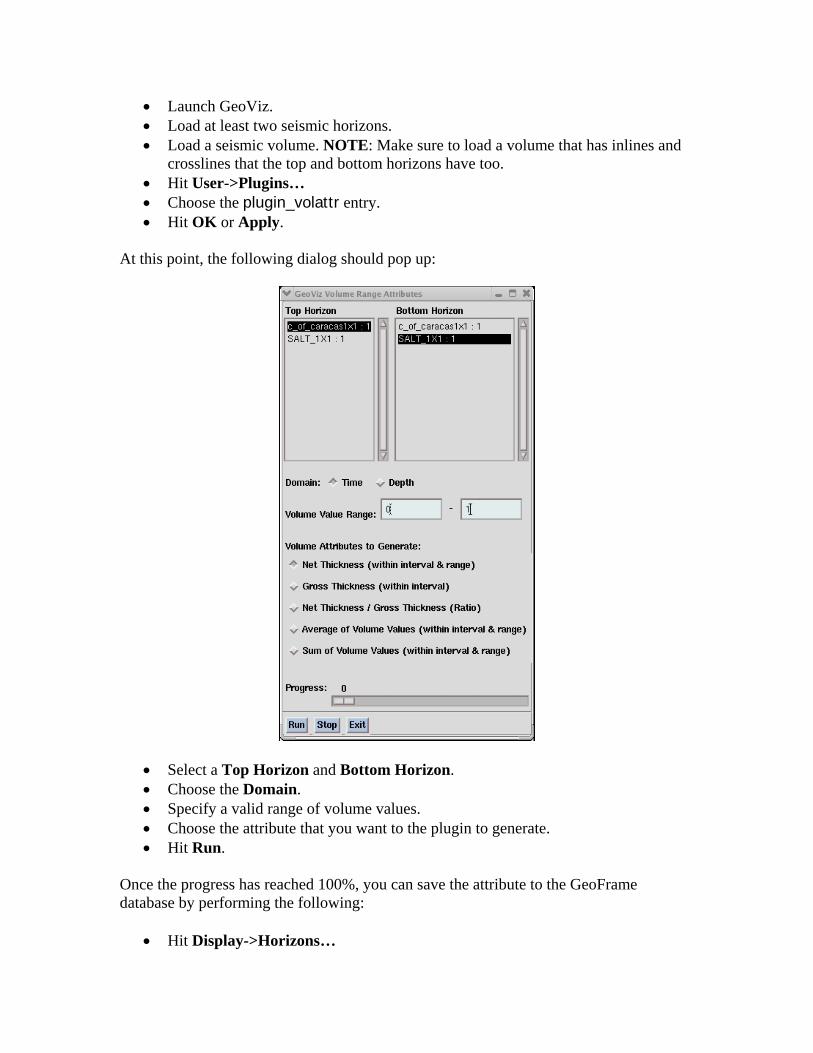
• Launch GeoViz. • Load at least two seismic horizons. • Load a seismic volume. NOTE: Make sure to load a volume that has inlines and

crosslines that the top and bottom horizons have too. • Hit User->Plugins… • Choose the plugin_volattr entry. • Hit OK or Apply.

At this point, the following dialog should pop up:

• Select a Top Horizon and Bottom Horizon. • Choose the Domain. • Specify a valid range of volume values. • Choose the attribute that you want to the plugin to generate. • Hit Run.

Once the progress has reached 100%, you can save the attribute to the GeoFrame database by performing the following:

• Hit Display->Horizons…

• Hit Save. • Enable the Save Draped Attribute toggle. • Enable the horizon name toggle and name it. The default is to write to the top

horizon. • Enable Overwrite. • Hit OK.

You have now saved the volume attribute.

NOTE: For every attribute that you want to save to the top horizon, you will need to execute the following sequence: 1. Setup the plugin parameters. 2. Hit Run. 3. Hit Save in the Display Horizons dialog. 4. Enable the Save Draped Attribute toggle, enable the horizon’s toggle and name it, and hit the Overwrite diamond. 5. Hit OK.

To view the attribute, you can use GeoViz or Basemap Plus: In GeoViz, get to the Modify Horizon/Fault dialog. From GF4.4 on, hit MB3 on the displayed horizon that we saved the attribute to, and select Property... Change the coloring to Ribbon, enable the Change Attribute toggle, and hit OK. A small dialog will pop up to prompt you to select an attribute. Choose the desired volume attribute and hit OK. For GeoViz versions before GF4.4, hit Tools->Modify…, select the appropriate horizon, and hit Modify… Then, change the attribute as in GF4.4 and on. In Basemap Plus, post the horizon and under Attribute choose the desired volume attribute before hitting OK or Apply.

GFDK Integration As mentioned earlier, the GFDK is the application programmers interface (API) allowing developers to directly access the Standard Data Model (SDM). The GFDK consists of the Application Data Interface (ADI), other associated API subsystems, and seismic data extensions. The ADI is subdivided into the Application Query Interface (AQI), the object-oriented relational data access subsystem, and the Application Port Utilities (APU), the bulk data access subsystem. The goal of this section is not to go in depth on the ADI, APU, and AQI, but to make you aware that they exist and point you to the correct document to help you write your own

GFDK programs using the GFDK APIs. Also, we give a brief explanation about some of the other documents on the GFDK Bookshelf. We conclude this section with an example on how to manipulate DataItems. For more information on the GFDK, please read the GFDK Integration document on the GeoFrame Bookshelf.

ADI, APU, and AQI The Application Data Interface (ADI) is a library of routines for interacting with GeoFrame’s geoscience database and bulk data storage systems. The ADI library presents an object-oriented or logical view of all data and, thus, frees the programmer from having to know how or where data is stored. The ADI accesses data objects, which are called DataItems (DIs), and their Attributes, which are used to characterize them and their relationships to other DIs. A Well DI, for example, contains Attributes such as a name, a creation date, and an identifier linking it to a particular Field. Examples of DIs include the following items:

Fields Wells Arrays Parameters Zones Horizons Faults

The Schlumberger Data Model lists all the DataItems and their attributes. The ADI library provides programmers with the following abilities:

Creating, querying, and deleting DIs Reading and writing DI attributes Locking and unlocking access to DIs manually in order to control concurrent access Specifying the boundaries within which operations on DIs are to be considered

atomic in order to control when modified data becomes visible to others Performing any meaningful conversion between supported units of measurement Specifying pre-defined or user-defined filters that are to be applied to DIs Determining when DIs have been modified by another program

Data Stores The geoscience bulk and non-bulk data available to the ADI are stored in an Oracle relational database and associated bulk data files (called Array Data Server or ADS files).

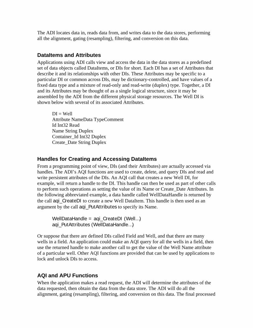
The ADI locates data in, reads data from, and writes data to the data stores, performing all the alignment, gating (resampling), filtering, and conversion on this data.

DataItems and Attributes Applications using ADI calls view and access the data in the data stores as a predefined set of data objects called DataItems, or DIs for short. Each DI has a set of Attributes that describe it and its relationships with other DIs. These Attributes may be specific to a particular DI or common across DIs, may be dictionary-controlled, and have values of a fixed data type and a mixture of read-only and read-write (duplex) type. Together, a DI and its Attributes may be thought of as a single logical structure, since it may be assembled by the ADI from the different physical storage resources. The Well DI is shown below with several of its associated Attributes. DI = Well Attribute NameData TypeComment Id Int32 Read Name String Duplex Container_Id Int32 Duplex Create_Date String Duplex

Handles for Creating and Accessing DataItems From a programming point of view, DIs (and their Attributes) are actually accessed via handles. The ADI’s AQI functions are used to create, delete, and query DIs and read and write persistent attributes of the DIs. An AQI call that creates a new Well DI, for example, will return a handle to the DI. This handle can then be used as part of other calls to perform such operations as setting the value of its Name or Create_Date Attributes. In the following abbreviated example, a data handle called WellDataHandle is returned by the call aqi_CreateDI to create a new Well DataItem. This handle is then used as an argument by the call aqi_PutAttributes to specify its Name. WellDataHandle = aqi_CreateDI (Well…) aqi_PutAttributes (WellDataHandle…) Or suppose that there are defined DIs called Field and Well, and that there are many wells in a field. An application could make an AQI query for all the wells in a field, then use the returned handle to make another call to get the value of the Well Name attribute of a particular well. Other AQI functions are provided that can be used by applications to lock and unlock DIs to access.

AQI and APU Functions When the application makes a read request, the ADI will determine the attributes of the data requested, then obtain the data from the data store. The ADI will do all the alignment, gating (resampling), filtering, and conversion on this data. The final processed

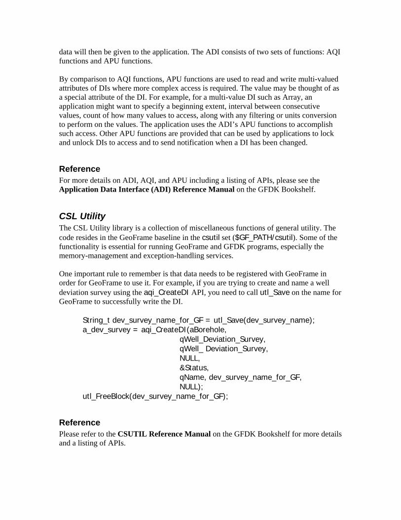
data will then be given to the application. The ADI consists of two sets of functions: AQI functions and APU functions. By comparison to AQI functions, APU functions are used to read and write multi-valued attributes of DIs where more complex access is required. The value may be thought of as a special attribute of the DI. For example, for a multi-value DI such as Array, an application might want to specify a beginning extent, interval between consecutive values, count of how many values to access, along with any filtering or units conversion to perform on the values. The application uses the ADI’s APU functions to accomplish such access. Other APU functions are provided that can be used by applications to lock and unlock DIs to access and to send notification when a DI has been changed.

Reference For more details on ADI, AQI, and APU including a listing of APIs, please see the Application Data Interface (ADI) Reference Manual on the GFDK Bookshelf.

CSL Utility The CSL Utility library is a collection of miscellaneous functions of general utility. The code resides in the GeoFrame baseline in the csutil set ($GF_PATH/csutil). Some of the functionality is essential for running GeoFrame and GFDK programs, especially the memory-management and exception-handling services. One important rule to remember is that data needs to be registered with GeoFrame in order for GeoFrame to use it. For example, if you are trying to create and name a well deviation survey using the aqi_CreateDI API, you need to call utl_Save on the name for GeoFrame to successfully write the DI.

String_t dev_survey_name_for_GF = utl_Save(dev_survey_name); a_dev_survey = aqi_CreateDI(aBorehole, qWell_Deviation_Survey, qWell_ Deviation_Survey, NULL, &Status, qName, dev_survey_name_for_GF, NULL); utl_FreeBlock(dev_survey_name_for_GF);

Reference Please refer to the CSUTIL Reference Manual on the GFDK Bookshelf for more details and a listing of APIs.

Application Runtime Control Application Runtime Control describes the dynamics of GeoFrame’s runtime control mechanism and the elements that constitute that mechanism. The elements are:

The entities that constitute the Application Runtime Control (ARC) database tables, such as modules, chains, products, and the attributes that define these tables. The tables contain information that the system must have to run program modules and manage their data. These tables also specify how modules are linked to form chains and products. The application programmer must create an SQL (Structured Query Language) file that inserts information about the program module in these tables.

The set of standard program module control commands that the user can execute from the application manager. The application programmer who designs a program module should specify code to be executed when these commands are issued.

A library of ARC functions that the application programmer can call from the program module to perform actions such as return status, execute a command, submit information to the database, abort, or exit the program, etc.

Application Initialization Command Line Arguments

Reference Please see the Application Runtime Control Reference Manual on the GFDK Bookshelf for more information including a listing of APIs.

ValueTypes The ValueTypes (VT) library is an extensible library of routines for tagging the types of data that move through the GeoFrame system and for performing some operations on the information returned. The library includes a variety of services for the following items:

Registered strings called atoms Symbolic functions Extended arrays called lists Data types called ValueTypes

Atoms An atom is a registered string that improves performance when doing symbolic processing. The C typedef for an atom is vt_Atom_t. In C, it behaves like String_t. In particular, you can call standard C functions like printf, strcat, and strlen on an atom. In the VT library, an atom is a unique 32-bit ID that is not dynamic and that should not be modified or freed. A naming convention is used for atoms. A C identifier that pertains to a particular atom is prefixed with the letter “q.” For example, an atom that has a value of “Name” would have a C identifier of qName.

Reference For a listing of APIs and more information on ValueTypes, please see the ValueTypes (VT) Reference Manual on the GFDK Bookshelf.

Units Library The Units Library is a library of routines for representing, managing, and accessing measurements and their units in the GeoFrame system. This library provides programmers with the following capabilities:

Create, access, and set unit systems Invoke an editor to inspect, change and save unit systems Determine if an entity is a valid unit or measurement, if units are convertible, or if

units are synonyms Retrieve units, measurements, conversion factors, dimensions of units or

measurements, unit synonyms, and storage or display units Convert data from one unit to another

Reference Please see the Units Library Reference Manual on the GFDK Bookshelf for more details and a listing of APIs.

SDM The goal of the Standard Data Model is to provide a foundation from which a coherent unified data model may be developed. The overall purpose of the data model is to provide an architecture for the database that allows many different applications to access the same data, while reducing the need to store the data in many different places. The data model must be as general as possible if it is to be flexible enough to encompass data from many different applications. A good data model is crucial when complex applications are tightly integrated and accessing the same data. Integrating applications by using an underlying data model reduces the amount of redundant data, and access to the data is more efficient. A relational database is used for the management of data. By allowing data to be stored in a central database instead of ‘flat files,’ the job pf the petroleum professional becomes much easier, with less chance of losing data, having to keep track of multiple copies of the same data (for example, inputting a datum with every piece of data for a well), or having to rebuild valuable information for each application. The main goal of using the data model is to reduce the time it takes to move the data among the numerous applications required to acquire, process, interpret, and so on the data.

Reference For more information, please see the SDM Data Modeling User Document on the GFDK Bookshelf. To access the SDM Data Item Report, perform the following at a GeoFrame xterm: >mozilla $GF_PATH/wk_sdm/direport/index.html

GFDK Example Program The GFDK Example Program teaches a developer how to create DataItems and manipulate various attributes related to fields, wells, and boreholes. The key concepts to grasp from the example are to learn how to use the aqi_xxx APIs (such as aqi_CreateDI, aqi_GetAttributes, etc.), GeoFrame memory management (such as utl_FreeBlock, utl_Save, etc.), and view the hierarchical structure of DataItems using the General Data Manager.

Description The gfdk_well_example executable is an example of how you can use the GFDK to write your own code to interact with GeoFrame. The program exemplifies how one can manipulate DataItems related to fields, wells, and boreholes in a GeoFrame project. Specifically, gfdk_well_example queries the GeoFrame database to see if a field named “Well_Manip_Field” exists. If it does not, then the program creates it. Then, gfdk_well_example attempts to select all wells that are in the “Well_Manip_Field” field that have a name that starts with “Well_Manip Well” and create a new well by appending a number to the end of the name. So for example, if the “Well_Manip_Field” has one well named “Well_Manip Well1”, then the program will create a new well named “Well_Manip Well2”. Next, a changeable X and Y location for the well are specified in creating a well position. Afterwards, the program creates a borehole with the same name as the well, and fills in the Borehole UWI attribute. Finally, an activity and array are created.

Building and Registering the GFDK Example Program In order to run gfdk_well_example, you need to build the executable and register it with your GeoFrame project. To build gfdk_well_example, you will need to add the gf_school directory to your GeoFrame work area by using the gfpath command in a GeoFrame xterm: >gfpath -add -set gf_school

Then, you will need to copy the gfdk_well_example.* files into the gf_school set that you added to your GeoFrame work area: >cp $GF_PATH/gf_school/gfdk_well_example.* gf_school/ Now, you should see at least three gfdk_well_example files in your gf_school directory: gfdk_well_example.c – Main C source file gfdk_well_example.lnk_def – Linker file gfdk_well_example.sql – SQL script At this point, you should be able to build gfdk_well_example, by issuing the following command at the GeoFrame xterm: >gbuild -update bin/gfdk_well_example Upon a successful build, you should see gfdk_well_example in your bin directory. If you decide that you want to make changes to the program, such as changing the X and Y location of the well, you can edit the gfdk_well_example.c file and then rebuild the program using gbuild. To register gfdk_well_example, you will login to your project with sqlplus and run the provided gfdk_well_example.sql script. To login to your project, you need to set the TWO_TASK environment variable to point to the correct database server (which can be found in the first combo box on the Login tab in proman). You will also need to know your project’s catalog (which also can be found on the Login tab in proman). So at the GeoFrame xterm, type the following: >setenv TWO_TASK database_server_name >sqlplus proj_name/proj_passwd After sqlplus has launched, you can register gfdk_well_example with your GeoFrame project: SQL>@gf_school/gfdk_well_example.sql catalog_name You may see some errors or warnings, which may be discouraging, but if you’ve run the script correctly, you can check that gfdk_well_example was registered properly by issuing the following commands: SQL>select name from module_cat; You should see GFDK_Well_Example Application listed.

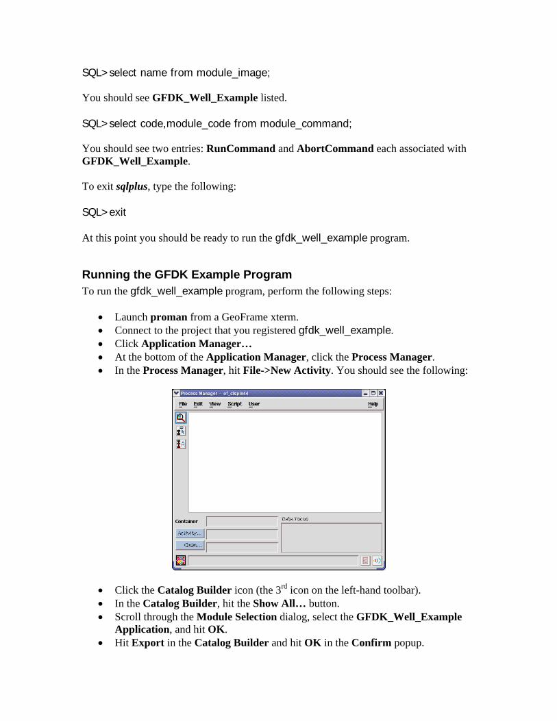
SQL>select name from module_image; You should see GFDK_Well_Example listed. SQL>select code,module_code from module_command; You should see two entries: RunCommand and AbortCommand each associated with GFDK_Well_Example. To exit sqlplus, type the following: SQL>exit At this point you should be ready to run the gfdk_well_example program.

Running the GFDK Example Program To run the gfdk_well_example program, perform the following steps:

• Launch proman from a GeoFrame xterm. • Connect to the project that you registered gfdk_well_example. • Click Application Manager… • At the bottom of the Application Manager, click the Process Manager. • In the Process Manager, hit File->New Activity. You should see the following:

• Click the Catalog Builder icon (the 3rd icon on the left-hand toolbar). • In the Catalog Builder, hit the Show All… button. • Scroll through the Module Selection dialog, select the GFDK_Well_Example

Application, and hit OK. • Hit Export in the Catalog Builder and hit OK in the Confirm popup.

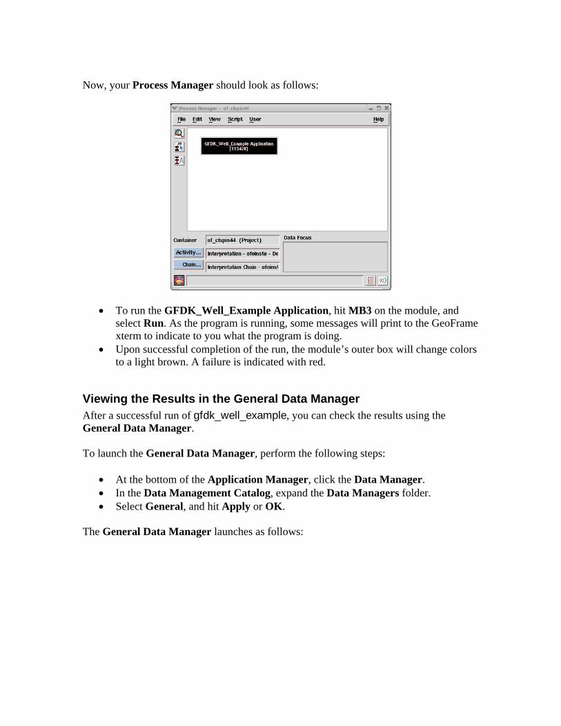
Now, your Process Manager should look as follows:

• To run the GFDK_Well_Example Application, hit MB3 on the module, and select Run. As the program is running, some messages will print to the GeoFrame xterm to indicate to you what the program is doing.

• Upon successful completion of the run, the module’s outer box will change colors to a light brown. A failure is indicated with red.

Viewing the Results in the General Data Manager After a successful run of gfdk_well_example, you can check the results using the General Data Manager. To launch the General Data Manager, perform the following steps:

• At the bottom of the Application Manager, click the Data Manager. • In the Data Management Catalog, expand the Data Managers folder. • Select General, and hit Apply or OK.

The General Data Manager launches as follows:

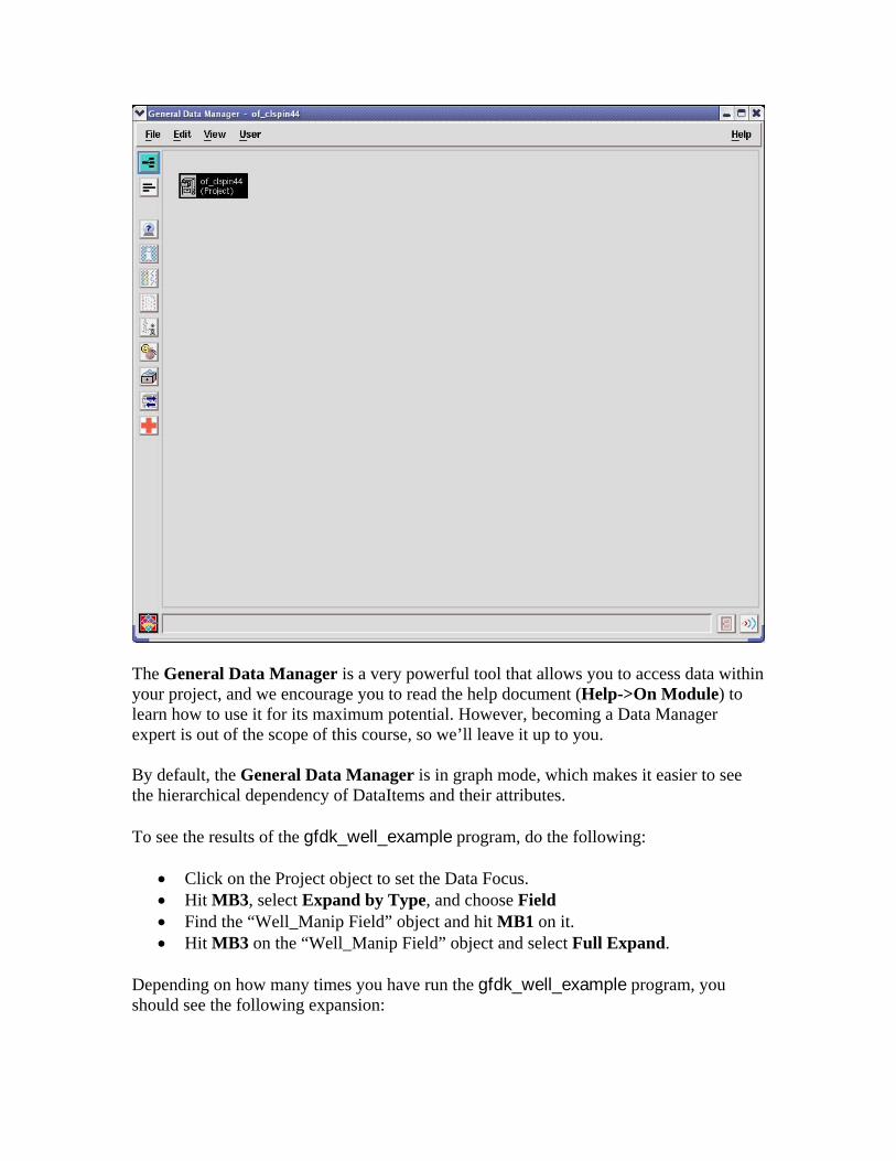
The General Data Manager is a very powerful tool that allows you to access data within your project, and we encourage you to read the help document (Help->On Module) to learn how to use it for its maximum potential. However, becoming a Data Manager expert is out of the scope of this course, so we’ll leave it up to you. By default, the General Data Manager is in graph mode, which makes it easier to see the hierarchical dependency of DataItems and their attributes. To see the results of the gfdk_well_example program, do the following:

• Click on the Project object to set the Data Focus. • Hit MB3, select Expand by Type, and choose Field • Find the “Well_Manip Field” object and hit MB1 on it. • Hit MB3 on the “Well_Manip Field” object and select Full Expand.

Depending on how many times you have run the gfdk_well_example program, you should see the following expansion:

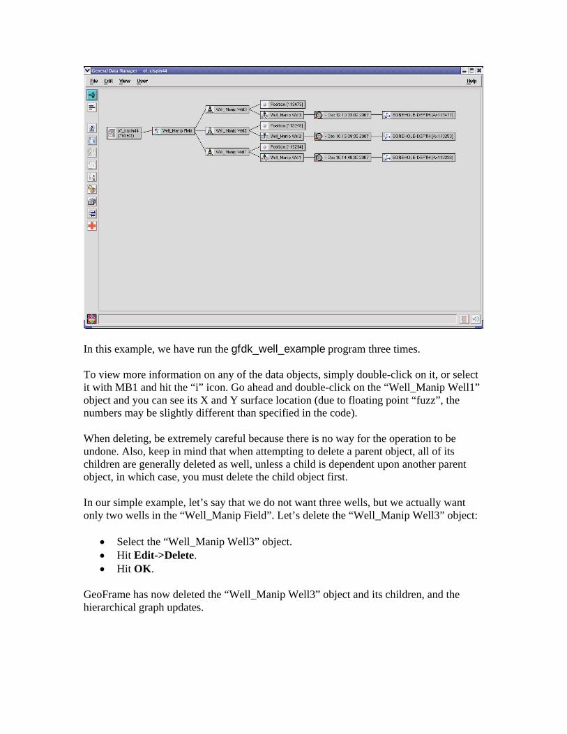
In this example, we have run the gfdk_well_example program three times. To view more information on any of the data objects, simply double-click on it, or select it with MB1 and hit the “i” icon. Go ahead and double-click on the “Well_Manip Well1” object and you can see its X and Y surface location (due to floating point “fuzz”, the numbers may be slightly different than specified in the code). When deleting, be extremely careful because there is no way for the operation to be undone. Also, keep in mind that when attempting to delete a parent object, all of its children are generally deleted as well, unless a child is dependent upon another parent object, in which case, you must delete the child object first. In our simple example, let’s say that we do not want three wells, but we actually want only two wells in the “Well_Manip Field”. Let’s delete the “Well_Manip Well3” object:

• Select the “Well_Manip Well3” object. • Hit Edit->Delete. • Hit OK.

GeoFrame has now deleted the “Well_Manip Well3” object and its children, and the hierarchical graph updates.

Wrap up Congratulations!!! You have made it through the Introduction to GFDK training course. In the class, you have learned about how to find the plethora of documentation included with GeoFrame and how to navigate in GeoFrame. Additionally, you have learned about the differences between the IESX DK, GeoViz On Connect, and the GFDK, and where to use which developer’s kit. Finally, we’ve provided you with several example programs so that you can learn how to write your own programs. We hope this guide was helpful to you. If you have further questions or would like to learn more than this course has to offer, we encourage you to delve into the documents found on the GFDK Bookshelf. For support, please contact your authorized Schlumberger field contact and have them submit a support ticket on your behalf.