GEWEX water vapor assessment (G-VAP) - World Climate ...

GEWEX water vapor assessment (G -VAP)

Final Report

December 2017 WCRP Publication No.: 16/2017

Bibliographic Information This report should be cited as: Schröder, M., Lockhoff, M., Shi, L., August, T., Bennartz, R., Borbas, E., Brogniez, H., Calbet, X., Crewell, S., Eikenberg, S., Fell, F., Forsythe, J., Gambacorta, A., Graw, K., Ho, S.-P., Höschen, H., Kinzel, J., Kursinski, E.R., Reale, A., Roman, J., Scott, N., Steinke, S., Sun, B., Trent, T., Walther, A., Willen, U., Yang, Q., 2017: GEWEX water vapor assessment (G-VAP). WCRP Report 16/2017; World Climate Research Programme (WCRP): Geneva, Switzerland; 216 pp. Contact Information All enquiries regarding this report should be directed to [email protected] or: World Climate Research Programme c/o World Meteorological Organization 7 bis, Avenue de la Paix Case Postale 2300 CH-1211 Geneva 2 Switzerland Cover Image Credits

Cover photography taken at mountain side of Mauna Kea by Marc Schröder in 2008: all rights reserved.

Copyright notice

This report is published by the World Climate Research Programme (WCRP) under a Creative Commons Attribution 3.0 IGO License (CC BY 3.0 IGO, www.creativecommons.org/licenses/by/3.0/igo) and thereunder made available for reuse for any purpose, subject to the license’s terms, including proper attribution.

Authorship and publisher’s notice This report was authored by the members of the GEWEX Water Vapor Assessment (G-VAP): M. Schröder, M. Lockhoff, L. Shi, T. August, R. Bennartz, E. Borbas, H. Brogniez, X. Calbet, S. Crewell, S. Eikenberg, F. Fell, J. Forsythe, A. Gambacorta, K. Graw, S.-P. Ho, H. Höschen, J. Kinzel, E. R. Kursinski, A. Reale, J. Roman, N. Scott, S. Steinke, B. Sun, T. Trent, A. Walther, U. Willen, Q. Yang. G-VAP is an initiative of the GEWEX Data and Assessment Panel (GDAP). G-VAP is co-chaired by Dr. Marc Schröder (Deutscher Wetterdienst, Offenbach, Germany) and Dr. Lei Shi (NOAA/NESDIS National Centers for Environmental Information, Asheville, USA), see www.gewex-vap.org and www.gewex.org/panels/gewex-data-and-assessments-panel . GEWEX is the Global Energy and Water cycle Exchanges (GEWEX) Core Project of WCRP, see www.gewex.org and www.wcrp-climate.org . WCRP is co-sponsored by the World Meteorological Organization (WMO), the Intergovernmental Oceanographic Commission (IOC) of UNESCO and the International Council for Science (ICSU), see www.wmo.int , www.ioc-unesco.org and www.icsu.org .

Disclaimer The designations employed in WCRP publications and the presentation of material in this publication do not imply the expression of any opinion whatsoever on the part of neither the World Climate Research Programme (WCRP) nor its Sponsor Organizations – the World Meteorological Organization (WMO), the Intergovernmental Oceanographic Commission (IOC) of UNESCO and the International Council for Science (ICSU) – concerning the legal status of any country, territory, city or area or of its authorities, or concerning the delimitation of its frontiers or boundaries. The findings, interpretations and conclusions expressed in WCRP publications with named authors are those of the authors alone and do not necessarily reflect those of WCRP, of its Sponsor Organizations – the World Meteorological Organization (WMO), the Intergovernmental Oceanographic Commission (IOC) of UNESCO and the International Council for Science (ICSU) – or of their Members. Recommendations of WCRP working groups and panels shall have no status within WCRP and its Sponsor Organizations until they have been approved by the Joint Scientific Committee (JSC) of WCRP. The recommendations must be concurred with by the Chair of the JSC before being submitted to the designated constituent body or bodies. This document is not an official publication of the World Meteorological Organization (WMO) and has been issued without formal editing. The views expressed herein do not necessarily have the endorsement of WMO or its Members. Any potential mention of specific companies or products does not imply that they are endorsed or recommended by WMO in preference to others of a similar nature which are not mentioned or advertised.

1

GEWEX water vapor assessment (G -VAP)

Final Report

M. Schröder, M. Lockhoff, L. Shi, T. August, R. Bennartz, E. Borbas, H. Brogniez, X. Calbet, S. Crewell, S. Eikenberg, F. Fell, J. Forsythe, A. Gambacorta, K. Graw, S.-P. Ho, H. Höschen, J.

Kinzel, E. R. Kursinski, A. Reale, J. Roman, N. Scott, S. Steinke, B. Sun, T. Trent, A. Walther, U. Willen, Q. Yang

Issue/Revision Index: 1.3

Date: 06 December 2017

2

Table of Contents

1 Executive summary ................................. .............................................................. 4

2 Introduction ...................................... .................................................................... 12

2.1 Overview 12

2.2 Scope, GEWEX needs and GCOS requirements 13

2.3 Scientific questions 15

2.4 Definitions 16

2.5 Information content and value of averaging kernels 17

3 Data records ...................................... ................................................................... 26

3.1 Overview on available satellite sensors 26

3.2 Potential sources of uncertainties 33

3.3 Data inventory 36

3.4 Overview of reference observations 38

4 Analysis of gridded data records .................. ..................................................... 43

4.1 Inter-comparison 43

4.2 Variability analysis 66

4.3 Homogeneity and trend analysis 86

4.4 Stability discussion 110

4.5 Consistency analysis 124

5 Intercomparison of data records from full archive . ........................................ 134

5.1 Data 134

5.2 Method 135

5.3 Results 135

5.4 Conclusions 139

6 Analysis of instantaneous data .................... .................................................... 140

6.1 Sampling 140

6.2 PDF analysis 146

3

6.3 Collocation 159

6.4 Inter-comparison 164

7 Conclusions ....................................... ................................................................ 180

8 Acknowledgment .................................... ........................................................... 183

9 References ........................................ .................................................................. 184

10 Appendix .......................................... ............................................................... 206

10.1 Brief description of data records 206

10.2 List of acronyms 213

4

1 Executive summary The executive summary provides an overview of the structure of the report and an

overview of the main results and conclusions. In the latter case links to corresponding sections are provided to ease access to specific details.

To date, a large variety of satellite based water vapour data records is available (see section 3.3, http://gewex-vap.org/?page_id=309 or http://ecv-inventory.com). Without proper background information and an understanding of the limitations of available data records, these data may be incorrectly utilised or misinterpreted. The need for quality assessments of Essential Climate Variables (ECVs) Climate Data Records (CDRs) is part of the GCOS guidelines for the generation of data products. Assessments in general give an overview of available data records and enable users to judge the quality and fitness for purpose of CDRs by informing them about the strengths and weaknesses of existing and readily available records. With this in mind, the GEWEX Data and Assessments Panel (GDAP) has initiated the GEWEX Water Vapor Assessment (G-VAP) which has the major purpose to quantify the current state of the art in water vapour products being constructed for climate applications and to support the selection process of suitable water vapour products by GDAP for its production of globally consistent water and energy cycle products. The assessment is geared to the needs of GDAP needs and to the requirements defined by GCOS which are recalled in section 2.2. They serve as baseline guidance to judge the fitness for purpose of the data records, in particular in terms of accuracy and stability. The usage of the products within GDAP activities essentially implied to study long-term data records. It is emphasised that data record specific user communities and application areas apply and that the data records have not been ranked. Within G-VAP all three products defined by GCOS to present the Essential Climate Variable water vapour were considered, namely upper tropospheric humidity (UTH), specific humidity (q) and temperature profiles (T) as well as total column water vapour (TCWV). The G-VAP report provides an overview of available satellite sensors and their general advantages and limitations as well as a data record inventory covering all available records of more than 10 years of temporal coverage. The corresponding tables are available for water vapour data records from satellites, in-situ and ground-based observations as well as from reanalyses (sections 3.1, 3.3, and 3.4). The tables include links to the section in which they have been analysed and a link to a webpage, a publication or a data fact sheet. This data fact sheet was explicitly developed for G-VAP and contains valuable information at a detailed level per data record. In order to guide the evaluation of data records within G-VAP, key science questions have been formulated. These questions are given in section 2.3 and a summary of answers to these questions is given in the conclusions (section 7).

In order to find answers to the G-VAP science questions three main classes of analyses were carried out:

• Analysis of long-term, gridded data records (section 4)

• Intercomparison of data records from full archive (section 5)

• Analysis of instantaneous data (section 6)

After a short summary, the applied methods and achieved results and conclusions are summarized for each of these three different classes of analyses.

The majority of long-term data records are affected by inhomogeneities. These inhomogeneities are typically caused by changes in the observing system and have a strong regional imprint. It is a major effort and challenge to increase the level of stability and to fully

5

understand the uncertainties on all regional scales which were induced by the methods applied to improve the stability. Steps in this direction need to involve (additional) reprocessing of input data, i.e., the generation of FCDRs, further improvements in retrieval design to handle changes in the observing systems and to handle regional issues and to reassess the improvement.

A series of regions with distinct features in differences among the data records and among trend estimates were observed. These regions include stratus regions, the poles and tropical land surfaces. In particular, at the top of stratus clouds and in the upper troposphere over tropical land areas, fairly large differences among the profile data records were observed. Dedicated evaluation studies are required to better understand these differences, the quality of the individual retrievals and the actual state of the climate and how it might have changed.

Moreover, gridded data records often suffer from missing information due to incomplete spatio-temporal sampling. The strength of the diurnal cycle of water vapour is typically small even on regional scales. However, several data records are clear sky or cloudy sky products. At a minimum, the clear sky products are impacted by sampling of the clear sky bias which is modulated by the diurnal cycle of clouds. In combination with orbital drifts artificial trends might be observed. Similar biases might occur in presence of rain. Sampling, retrieval design and increased uncertainties at small and large values might hamper a proper analysis of the PDF of water vapour, its extremes and how the PDF and the extremes change in a changing climate. Joint analyses using various parameters and various observing systems are needed to better constraint associated uncertainties.

Analysis of long-term, gridded data records

Applied methods and analysed data records included:

• Intercomparison

o TCWV: CFSR, ERA20C, ERA-Interim, HOAPS, JRA55, MERRA, MERRA2, nnHIRS, NVAP-M Climate, NVAP-M Ocean, SSM/I (REMSS)

o Profiles: CFSR, ERA20C, ERA-Interim, JRA55, MERRA, MERRA2, nnHIRS, NVAP-M Climate

o UTH: AMSU-B, HIRS, METEOSAT

• Variability

o TCWV: CFSR, ERA-Interim, HOAPS, MERRA, NVAP-M Climate, SSM/I (REMSS), EC Earth, MPI ESM

o UTH: AMSU-B, HIRS, METEOSAT

• Homogeneity and trend estimates

o TCWV: CFSR, ERA20C, ERA-Interim, HOAPS, JRA55, MERRA, MERRA2, nnHIRS, NVAP-M Climate, NVAP-M Ocean, SSM/I (REMSS)

o Profiles: CFSR, ERA20C, ERA-Interim, JRA55, MERRA, MERRA2, nnHIRS, NVAP-M Climate

• Stability

o TCWV: HIRS NOAA, HOAPS

• Consistency

o AMSU-B, CFSR, ERA-Interim, HIRS, HOAPS, MERRA, NVAP-M Climate, SSM/I (REMSS)

6

Results from intercomparison studies provide a good overview of differences among the various long-term (more than 20 years, starting in the 1980s) data records. The comparisons were carried out relative to the ensemble mean. In response to an essential GEWEX need, the assessment analysed the stability of the long-term data records. Here it was differentiated between the degree of homogeneity, that is, the presence of breakpoints, and stability, that is, the change of the bias relative to a reference over time. Thus, Hovmöller diagrams, homogeneity test results and trend estimates were considered. Trend estimation needs to be understood in this context as an intercomparison toolas G-VAP does not assess climate change. Interesting agreements/disagreements were observed between standard deviations relative to ensemble means and differences among trend estimates as well as between TCWV, UTH and profiles. The degree of homogeneity is largely impacted by breakpoints. Thus, the stability has been assessed using exemplary data only. Also, Hovmöller diagrams, homogeneity tests and trend estimation are affected by climate variability. For this reason, the correlations to major climate indices, e.g., related to ENSO, to NAO and to PDO and the associated consistency were assessed as well. Finally, the long-term, gridded data records have been compared to long-term multi station radiosonde data archives. Here time series of differences at GRUAN sites are shown, with two objectives: first, to further strengthen the stability analysis and second, to link the analysis of gridded data records to the analysis of instantaneous profile data.

The following list provides conclusions for the analysis of long-term, gridded data records together with links to the sections in which more details can be found:

TCWV

• The intercomparison of long-term TCWV data records revealed largest differences over tropical land regions (e.g., Central Africa and South America), deserts (e.g., Sahara), mountainous regions and the poles. The intercomparison of time series exhibited artefacts and breakpoints in the majority of data records (section 4.1.1).

• On a global ice-free ocean scale the TCWV trend estimates exhibit large differences (ranging from -0.11±0.09 to 1.21±0.16 kg/m2/decade considering 10 data records of more than 20 years temporal coverage) and are often significantly different among the different data records (section 4.3.1).

• Except for HOAPS and REMSS (within uncertainty estimates) all data records exhibit regression values outside the theoretically expected range. This is an indication of issues in long-term stability (section 4.3.1).

• Regions with maxima in mean absolute difference of the TCWV trend estimates largely coincide with the maxima in ensemble standard deviations (section 4.1.1). The most pronounced regions are again tropical land regions (e.g., Central Africa and South America), deserts (e.g., Sahara), mountainous regions and the poles (section 4.3.1).

• The differences in trend estimates in these regions and over global ice-free ocean were found to be caused by breakpoints or series of breakpoints. The break size can reach values of almost 2 kg/m2. In most cases these breakpoints coincide temporally with changes in the observing system. The time of occurrence, sign, and step size of breakpoints are typically a function of region and data record. The majority of these breakpoints are not evident when comparisons to the HomoRS92 data record were carried out. One reason is that areas with distinct differences in trend estimates are not covered with stations. It is obviously important to verify the homogeneity and stability on global and all regional scales (section 4.3.1).

• Noise and autocorrelation determine the temporal length (time-to-detect, TTD) of a data record which is needed to detect an expected trend. It is shown that uncertainties higher than 3% result in TTDs above 15 years. Advanced water vapour products from AIRS and IASI exhibit uncertainties in the extreme bin which exceed 5%. This emphasises the value

7

of analysing uncertainties as a function of dependent variables such as, in this case, TCWV (section 4.3.1). It is further recommended to characterise the TTD by taking into account the vertical resolution and sensitivity of satellite sounders (section 2.5).

• All long-term TCWV data records are highly correlated with ENSO and exhibit different levels of correlation with other climate indices. The correlations of two considered climate models do not differ significantly from the satellite based TCWV data records when SST-based indices were analysed (section 4.2.1).

• The identification of regions with significant correlation to climate indices, common to all data records, is a potentially valuable approach to guide climate model evaluation (section 4.2.1), thus enhancing the value and usability of satellite data records.

Spedific humitiy and temperature profiles

• Regions of maximum differences among the profile data records (that is maximum ensemble standard deviations) do not typically coincide with those of TCWV, except for maxima at the poles and over Central Africa. Regions with local maxima typically occur over the ocean, e.g., the stratus regions (section 4.1.2).

• Maxima in trend differences of profile data generally occur over the ocean, except for Central Africa. The distinct ocean regions are the stratus region and the southern edge of the ITCZ. Regions of maximum standard deviation and of maxima in trend differences generally do not coincide, except for stratus regions off the coast of South Africa. Profiles of trend estimates, based on regional averages over the tropics and the northern and southern hemispheres, are typically significantly different. Differences are smallest near the surface (section 4.3.2).

• Stratus regions appear as local maxima in ensemble standard deviations and in trend differences in water vapour and temperature profiles. Position of cloud top and amount of water vapour above cloud top are major differences. Also, the differences in the upper troposphere overwest Africa are comparably large over tropical land areas.

• Vertical and spatial features in intercomparison and trend estimation results are often different between temperature and water vapour profiles.

• As for TCWV the profile data records exhibit inhomogeneities on regional scale (section 4.3.2).

UTH

• A dry bias of more than 20% was observed between IR and microwave based UTH products. This can be explained by a clear sky bias, i.e., a systematic bias caused by differences in sampling. Collocated HIRS and Meteosat UTH products exhibit a systematic difference of >20% which is largely caused by the utilisation of different weighting functions during retrieval design.

• The UTH products exhibit similar amplitudes and associated variability after 1998. The potential of using UTH to monitor long-term changes in large-scale atmospheric circulation and for locating teleconnections was shown (section 4.2.2).

• During El Nino, absolute water vapour contents increase significantly over large areas of the tropics. In contrast UTH decreases over large areas of the tropics corresponding to changes in the general circulation. The increase in UTH is confined over a small area at the central eastern equatorial Pacific. Thus, UTH and TCWV/profiles are in opposite phase when looking at tropical averages. Note that complex lag (between parameter and ENSO index) correlations are found as well (section 4.5).

8

General

• A careful recalibration and intercalibration of raw data records, retrieval harmonisation/improvements and refined assimilation schemes are key elements to increase the level of homogeneity and stability. A sound uncertainty estimation is required as well and such efforts should be carried out in conjunction with a reassessment of the achieved change in quality (section 4.3.1).

Intercomparison of data records from the full archive

Considered data records: AIRWAVE, AMSRE (JAXA), AMSRE (REMSS), ATOVS (CM SAF), CFSR, EMiR, ERA20C, ERA-Interim, GOME GlobVapour, HOAPS, JRA55, MERIS, MERRA, MERRA2, MODIS AQUA, nnHIRS, NVAP-M Climate, NVAP-M Ocean, SSM/I (REMSS), SSMI+MERIS, TMI (REMSS), UWHIRS

Ten long-term data records are available to G-VAP. However, the number of data records which have at least a temporal coverage of 10 years is much larger and exceeds twenty-five. In order to provide a first assessment of the full archive these data records have been intercompared relative to the ensemble mean. Also differences among ensembles based on weather types such as clear sky and cloudy sky are presented. We conclude that the weather type analysis does not seem to highlight differences among the different weather types because the internal variability of the weather types is generally larger than the differences between the bins.

Analysis of instantaneous data

Applied methods and considered data records included:

• Sampling

TCWV: COSMIC, GNSS, NVAP-M Ocean, SSM/I REMSS

• PDF

Profiles: AIRS, CFSR, COSMIC, ECMWF IFS, ERA-Interim, MERRA, NCEP FNL

• Collocation

• Intercomparison

Profiles: AIRS, ECMWF IFS, HIRS NOAA, IASI NOAA

The focus here is on the comparison of profiles using instantaneous data from recent years. The profile quality in the upper troposphere, near the surface and over the ocean is assessed by considering bias-corrected and quality controlled RS92 radiosondes and GRUAN radiosondes. In order to build a bridge between the analysis of long-term gridded and instantaneous data sampling issues arising from diurnal sampling, gap filling, retrieval constrains and the added value / the need for analysis of PDFs are discussed. The collocation aspect is discussed with focus on collocation uncertainty. In the following conclusions are provided, again with links to corresponding sections:

• Comparison results are strongly affected by sampling differences. It is recalled that the clear sky (dry) bias, that is, the difference between TCWV from clear sky and clear + cloudy sky observations is typically -2 kg/m2 and can regionally exceed values of -7 kg/m2 or even -10 kg/m2, also depending on the considered data records (literature review in section 6.1.2). Also for UTH a clear sky (dry) bias is observed with typical values of – 9

9

%RH (or >25% relative) and maximum values of -30 %RH (50% relative) (section 4.1.3 and section 6.1.2). Data gaps can occur in presence of strong rain events and can be filled by using information from surrounding pixels. This way the PDF is filled at the wet end, leading to larger values (up to 1.5 kg/m2 or 4% for TCWV, section 6.1.3). Finally, the uncertainty of an SSM/I based TCWV retrieval has been analysed as function of LWP and precipitation amounts using GPS RO data as reference. An increase in bias and RMS is evident in presence of rain (section 6.1.6). Finally, the bias in TCWV due to diurnal sampling issues is <0.1 kg/m2 on a global scale and hardly exceeds 10% bias when looking at individual locations. It seems that the relatively large differences between the various data records are not predominantly affected by the diurnal cycle of water vapour but the diurnal cycle of clouds and thus the sampling of the clear sky bias explains the observed differences (section 6.1.4).

• The value, if not the need, of computing and analysing PDFs is shown in section 6.2. A large diversity in density at the high end of the PDF is shown (547 hPa, specific humidity). None of the analyses or climate model PDFs exhibits the peak at the dry end of the PDF (725 hPa). It is strongly recommended not to interpolate to lower resolutions in this approach. In general, it needs to be kept in mind that the PDF of water vapour is not Gaussian and thus, the consideration of mean values blurs issues in the retrieval and might not be representative.

• Comparison results are further impacted by collocation uncertainties (section 6.3). It is shown that variability scales are as low as 2 km and 10 min. New approaches are briefly introduced that reach comparison results within accuracy of the reference observations and that allow the estimation of the collocation uncertainty.

• The information content (resolution, degrees of freedom, vertical coverage) of sounder observations requires careful attention. A potential lack of sensitivity in humidity sounding by hyperspectral sounders is evident at near surface layers and in the tropopause and above (section 2.5). The provision of averaging kernels, a priori information and error covariance matrices are highly recommended (sections 2.5 and 3.2).

• A new approach to analyse the quality of water vapour profile data records was developed and consists of the following steps: proper use of averaging kernels and uncertainty estimates from reference and retrieval, consistency test, z-test, and uncertainty estimation of the bias between retrieval and reference. The added value of consistency and z-testing was shown via uncertainty analysis. The presented results point to the need for accurate surface characterisation in order to overcome the ambiguity in IR based near surface retrievals over land (section 6.4.2).

• Based on results from the well established evaluation tool NPROVS+ it was shown that the performance of advanced retrievals such as from AIRS, IASI and HIRS and analysis systems such as from ECMWF decreases with height. It further seems that the satellite retrievals have reduced sensitivity in dry atmospheres and lower quality over non-tropical land than over tropical oceans. GRUAN radiosondes have been used as reference. It is argued that the uncertainty of GRUAN humidity data is too large at large humidity values. Feedback to the GRUAN Lead Centre was provided and in general such comparison results can also provide valuable feedback to the reference observation operator (section 6.4).

In this report, differences in advanced and freely available water vapour data records were identified, documented and to a large extend explained. This will allow data record providers to easily assess their data record’s improved quality and stability in future updates given the results presented here. In fact, lessons learned about regional changes have already provided guidance for future improvements of data records. One of the major advantages of an effort like G-VAP is to suggest and encourage improvements to data records included in the G-VAP analysis. Discussions between G-VAP participants over the last years have allowed participants

10

to receive new perspectives on their work. Analyses of data records by outside, independent scientists willing to provide critical feedbacks are of great benefit. For example, the discovery of the regional breakpoints in NVAP-M over the Sahara by G-VAP members has prompted further investigation by the NVAP-M team into the challenges of using infrared data over a surface with variable emissivity and a variable atmosphere that is often impacted by dust storms. These factors will be addressed in future production efforts.

Recommendations

The following recommendations have been compiled on basis of the discussions at the G-VAP workshops. These consensus results have been made available via the minutes of meetings which are available at www.gewex-vap.org. Finally, minor updates have been included following discussions at the GDAP meeting in fall 2016. References to corresponding sections are given as well.

• CGMS, Space Agencies: Improve upon current satellite profiling capabilities with goals of providing high precision and long term stability, with sufficient vertical resolution, complete, unbiased global sampling and independency of models (sections 4.3.2.3 and 6.2).

• CGMS, Space Agencies: Dedicated validation archive for all water vapour sensors, also including ship based RS (sections 4.1, 6.4).

• CGMS, WMO, GRUAN: Aim at the sustained generation and development of a stable, bias corrected multi-station radiosonde archive including reprocessing of historical data (section 6.4).

• CGMS, WMO: Achieve consistency among reference observing systems and sustain corresponding services (section 6.3).

• WMO, GCOS: Oppose and balance user, scientific and product requirements with focus on climate analysis.

• Space Agencies: Need for continental high quality satellite data records. • Space Agencies: Need for inter-calibrated radiance/brightness temperature data

records and homogeneously reprocessed instantaneous satellite data records (sections 4.2.2, 4.3, 4.4).

• Space Agencies, GEWEX: Provide water vapour transport product in order to analyse atmospheric dynamics and to evaluate the constancy of relative humidity.

• Space Agencies, PIs: Develop and provide PDF based climatology of satellite-based radio-occultation data (section 6.2).

• Space Agencies, PIs: Provide averaging kernels, a priori state vectors and associated error covariance matrices together with the release of profile products (section 2.5).

• Space Agencies, PIs, G-VAP: Estimate and provide uncertainty information and assess uncertainty estimates, also as function of total amounts and other dependent parameters (sections 3.2, 4.3.1.4, 6.4).

• Space Agencies, PIs, G-VAP: Improve stability of long-term data records and (re)assess improvement in stability (sections 4.3, 4.4).

• Space Agencies, PIs: Provide information on input to data records such as precise start and stop dates and number of observations as function of time and input data type (section 4.3).

• GEWEX, SPARC, G-VAP, WAVAS: Joint WAVAS and G-VAP analysis of data records covering the upper troposphere and lower stratosphere using the same methodology.

• GRUAN: Include station over tropical land (sections 4.1, 4.3, 6.4.2). • GRUAN: Reassess the uncertainty estimates at large humidity values (section 6.4). • GRUAN: Provide estimates of the correlation uncertainty between levels or guidance

11

on how to compute it from information already available (ideally the covariance matrix of uncertainties is provided, section 6.3).

• GEWEX: Continuous support to G-VAP, beyond acceptance of first report. • G-VAP, Space Agencies, PIs: Enhance quality analysis of profile data records over

open ocean, in particular over high pressure areas/subsidence areas and stratus (sections 4.1.2, 4.3.2).

• G-VAP, Space Agencies, PIs: Analyse differences between observations under all-sky as well as cloudy and clear sky conditions (sections 4.1.1, 4.1.2, 6.1).

• G-VAP: Reassess the TTD of humidity profile data by taking into account the vertical resolution and sensitivity and the characteristics of the PDF at certain levels/layers (section 2.5, section 6.2).

• G-VAP: Assess the joint effect of orbital drift, clear sky sampling/bias and the diurnal cycle of clouds on biases and how this might change with climate change (section 6.1).

• G-VAP supports the ITSC-20 recommendation on the reinstallation of the TPW ARM station.

• G-VAP supports the ITSC-20 initiative to collect SRF data in common format at a common location.

• G-VAP supports the concluding remarks from the Joint workshop on uncertainties at 183 GHz.

In addition to the main conclusions and recommendations an overview of the main output from G-VAP is given in section 2.1.

12

2 Introduction

2.1 Overview

M. Schröder (DWD)

Several dedicated studies have been carried out to characterise the quality of individual and/or subsets of freely available water vapour data records. This was achieved in various ways: intercomparison (e.g., Divakarla et al., 2014; Schröder et al. 2013; Sohn and Smith 2003), comparison to ground-based / in-situ data (e.g., Bedka et al., 2010; Lindstrot et al., 2014; Rienecker et al., 2011) or both (e.g., Bühler et al., 2012; Reale et al., 2012), and intercomparison of trend estimates (e.g., Dessler and Davis, 2010; Mears et al., 2007; Mieruch et al., 2014; Trenberth et al., 2005). Here only a few examples are given. A far more comprehensive overview is given in Kämpfer (2012) and at http://www.watervapour.org, with an extensive literature database with entries up to 2009. Wulfmeyer et al. (2015) provide an overview of precision and bias for various spaceborne observing system types with respect to humidity and temperature profiling (their tables 2 and 3). It is interpreted that this overview is based on a literature review and is mainly concerned about retrieval uncertainty. Results from these and other studies are often difficult to compare and interprete because the considered data records might have been subjected to different types of preprocessing, different metrics might have been considered, or different periods and/or regions were analyzed. To our knowledge a consistent analysis of the quality of all mature and freely available long-term data records has not been carried out to date. This gap is filled by G-VAP. The overall goal of the GEWEX water vapor assessment (G-VAP) is to characterise freely available satellite data records. The characterisation is guided by a set of science questions. Finding answers to these questions is done in different ways in this report: analysis of data from full archive, analysis using a subset of data records, and literature review.

This WCRP report on G-VAP is structured as follows: after recalling the scope, the GEWEX needs, GCOS requirements and the scientific questions, the applicable sensors and data records are briefly introduced and a general discussion of uncertainties is given. The core of the report is separated into three parts where results from the analysis of long-term (more than 20 years, start in the 1980s or earlier) gridded data records (Level 3 or higher, section 4), of short-term (minimum of 10 years) gridded data records (section 5) and of instantaneous (Level 2) data records (section 6) are presented. Section 4 has a strong focus on the characterisation of homogeneity and stability while section 6 concentrates on systematic and random uncertainties associated with retrievals. An overview of uncertainties arising from sampling and collocation is also given in section 6.

Generally, TCWV, water vapour and temperature profiles as well as UTH were analysed but not all those parameters have been assessed in each section. Whenever feasible the full suite of long-term data records has been analysed. However, a series of case studies or studies using a subset of data records were carried out. Section 3.3 provides an overview of available data records. It also shows which data record and parameter are analysed in which section.

Section 7 provides answers to the G-VAP science and technical questions and additional conclusions.

Teams of authors have drafted each section as stand alone reports. If not included as a whole, summaries are included here together with a link to the complete report. In such cases the reports are available at http://www.gewex-vap.org. Individual sections may include definitions of e.g. uncertainty different from definitions given in section 2.4.

The following list provides an overview on output from G-VAP:

13

• Scientific papers in peer reviewed journals

(see section 9),

• WCRP report on G-VAP

(available online at www.gewex-vap.org -> DISSEMINATION -> G-VAP REPORT),

• Stand alone (sectional) reports and documents

(available online at www.gewex-vap.org-> DISSEMINATION -> DOCUMENTS),

• Recommendations

(see section 1),

• Information data base

(available online at www.gewex-vap.org-> DATA RECORDS),

• Regridded data records

(available online at www.gewex-vap.org -> G-VAP DATA ARCHIVE).

2.2 Scope, GEWEX needs and GCOS requirements

M. Schröder (DWD)

The need for quality assessments of Essential Climate Variables (ECVs) Climate Data Records (CDRs) is part of the GCOS guidelines for the generation of data products. The assessment process shall give an overview of available data records and enable users to judge the quality and fitness for purpose of CDRs by informing them about the strengths and weaknesses of existing and readily available records. This is achieved by inter-comparison and evaluation, and by providing reasons for differences and limitations where possible. Assessments of data records related to the global energy and water cycles became an integral part of GEWEX activities over the last decades. The GEWEX Radiation Panel (GRP, renamed to GEWEX Data and Assessments Panel - GDAP) has initiated the GEWEX Water Vapor Assessment in 2011, further on referred to as G-VAP. The major purpose of G-VAP is to1:

• Quantify the current state of the art in water vapour products being constructed for climate applications, and by this,

• Support the selection process of suitable water vapour products by GDAP for its production of globally consistent water and energy cycle products.

The optimum GEWEX needs on satellite based temperature and humidity products are2:

• Global coverage, • 3 hourly temporal resolution, • 10 km spatial resolution, • Availability from 1979 to present,

1 http://www.gewex.org/gewexnews/May2011.pdf 2 http://due.esrin.esa.int/meetings/meetings247PRE.php

14

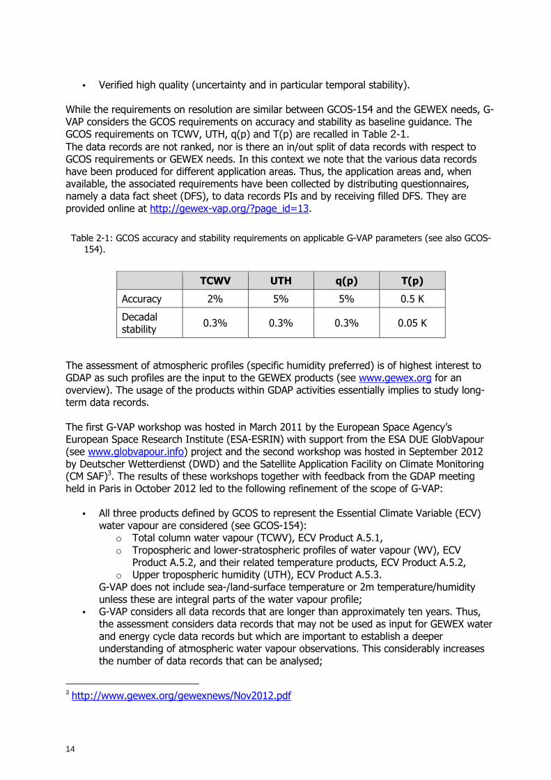
• Verified high quality (uncertainty and in particular temporal stability). While the requirements on resolution are similar between GCOS-154 and the GEWEX needs, G-VAP considers the GCOS requirements on accuracy and stability as baseline guidance. The GCOS requirements on TCWV, UTH, q(p) and T(p) are recalled in Table 2-1. The data records are not ranked, nor is there an in/out split of data records with respect to GCOS requirements or GEWEX needs. In this context we note that the various data records have been produced for different application areas. Thus, the application areas and, when available, the associated requirements have been collected by distributing questionnaires, namely a data fact sheet (DFS), to data records PIs and by receiving filled DFS. They are provided online at http://gewex-vap.org/?page_id=13.

The assessment of atmospheric profiles (specific humidity preferred) is of highest interest to GDAP as such profiles are the input to the GEWEX products (see www.gewex.org for an overview). The usage of the products within GDAP activities essentially implies to study long-term data records. The first G-VAP workshop was hosted in March 2011 by the European Space Agency’s European Space Research Institute (ESA-ESRIN) with support from the ESA DUE GlobVapour (see www.globvapour.info) project and the second workshop was hosted in September 2012 by Deutscher Wetterdienst (DWD) and the Satellite Application Facility on Climate Monitoring (CM SAF)3. The results of these workshops together with feedback from the GDAP meeting held in Paris in October 2012 led to the following refinement of the scope of G-VAP:

• All three products defined by GCOS to represent the Essential Climate Variable (ECV) water vapour are considered (see GCOS-154):

o Total column water vapour (TCWV), ECV Product A.5.1, o Tropospheric and lower-stratospheric profiles of water vapour (WV), ECV

Product A.5.2, and their related temperature products, ECV Product A.5.2, o Upper tropospheric humidity (UTH), ECV Product A.5.3.

G-VAP does not include sea-/land-surface temperature or 2m temperature/humidity unless these are integral parts of the water vapour profile;

• G-VAP considers all data records that are longer than approximately ten years. Thus, the assessment considers data records that may not be used as input for GEWEX water and energy cycle data records but which are important to establish a deeper understanding of atmospheric water vapour observations. This considerably increases the number of data records that can be analysed;

3 http://www.gewex.org/gewexnews/Nov2012.pdf

Table 2-1: GCOS accuracy and stability requirements on applicable G-VAP parameters (see also GCOS-154).

TCWV UTH q(p) T(p)

Accuracy 2% 5% 5% 0.5 K

Decadal stability

0.3% 0.3% 0.3% 0.05 K

15

• The assessment considers data records that are provided by assessment participants and that are readily available and well documented;

• The assessment focuses on overall characteristics of participating satellite and reanalysis data records as determined from inter-comparisons and comparisons against in situ observations and ground-based products;

• The consistency of TCWV and UTH with the profile data is studied as well; • Long-term Level-3 (gridded products) products are analysed on different time and

space scales in order to get an overview of issues in Level-3 products. These issues can then be studied in more detail using Level-2 and/or Level-1 data and by dedicated Level-2 data comparisons employing high quality satellite and ground-based observations;

• G-VAP built up a database including collocated products and “reference” data of sufficient quality, in particular long-term stability, which serves as main repository for the current assessment and which will be also useful for the development of improved products.

• G-VAP pursues information exchange with the SPARC water vapour activity, with SPARC focusing on the stratosphere and G-VAP focusing on the troposphere.

2.3 Scientific questions

M. Schröder (DWD)

Following presentations and discussions at the first GDAP meeting in October 2012 key questions for the evaluation of data records have been formulated. The questions below determine the metric to identify strengths and limitations, to analyse differences and to find reasons for distinct differences and limitations. The science questions are: Q1)

a) How large are the differences in observed temporal changes in long-term satellite data records of water vapour on global and regional scales?

b) Are the observed temporal changes and anomalies, on global and regional scale, in line with theoretical expectations?

c) Are the differences in observed temporal changes within uncertainty limits? d) What is the degree of homogeneity (breakpoints) and stability of each long-term

satellite data record? e) How can we enhance value and usability of the satellite data records (e.g., through

analysis of consistency in climate related features such as position and strength of dry zones, regional annual cycles, and El Nino response)?

Q2) What is the degree of consistency among the products? Q3)

a) Do the satellite data records exhibit areas of distinct quality and how can the distinct differences and limitations be explained?

b) What is the quality of long-term satellite WV products in the lowermost part of the atmosphere and in the upper troposphere?

c) What is the quality of long-term satellite TCWV and WV products over ocean where ground-based and in-situ observations are rarely available?

16

Q4) What are the differences in quality between satellite products and products from reanalysis and are the observed differences significant? The technical question is: Q5) How easily can the satellite data records be downloaded, read and understood? This report provides answers to these questions and a summary of the answers is given in section 7.

2.4 Definitions

M. Lockhoff (DWD), lead authors

Provided below are the definitions of terms used throughout this report.

Total column water vapour (TCWV) Vertical integral of absolute water vapour amounts from the ground to the top of the atmosphere in unit kg/m2

Water vapour / Temperature profiles

Specific humidity (g/kg) and temperature (K) values at pressure levels. NVAP-M and UW HIRS contain layer integrated water vapour in unit kg/m2 at 4 and 3 layers, respectively. In case spatial maps are analysed the following levels are considered: 1000 hPa, 700 hPa, 500 hPa, and 300 hPa.

Upper Tropospheric Humidity (UTH)

Mean relative humidity integrated over a broad layer in the upper troposphere. Layer thickness and position depends on atmospheric condition, channel characteristics and weighting functions used for integration.

Homogeneity

Following the definition of Köppen & Geiger (1936) time series are considered to be homogeneous, if their variations are caused only by meteorological influence. Inhomogeneities may arise from: • Satellite changes, • Instrument changes and calibration, • Observation and sampling time, • Orbital drift, • Algorithm changes, • etc. Within the report a homogeneous data record does not contain significant breakpoints.

Stability

“The user requirement for stability is in general a requirement on the extent to which the error of a product remains constant over a long period...The relevant component of error of a product for climate application is often the systematic component defined by the mean error... Values

17

quoted under the heading “stability” in this document refer to the maximum acceptable change in systematic error per decade... Stability of the random component may also be a requirement...” [GCOS-154] “Stability may be thought of as the extent to which the accuracy remains constant with time. Over time periods of interest for climate, the relevant component of total uncertainty is expected to be its systematic component as measured over the averaging period. Stability is therefore measured by the maximum excursion of the difference between a true value and the short-term average measured value of a variable under identical conditions over a decade. The smaller the maximum excursion, the greater the stability of the data set.” [Dowell et al., 2013] In the report stability is defined as the change of the systematic uncertainty over time relative to a reference if not defined differently.

Correlation Here the Pearson correlation coefficient is used if not stated differently.

Long-term data records All data records covering time series with a minimum record length of 20 years and with a start date in the 1980s.

Short-term data records All data records covering time series longer than 10 years.

2.5 Information content and value of averaging kern els

T. August (EUMETSAT), T. Trent (U. Leicester)

The notions of vertical sensitivity and vertical resolution applied to space-borne sounding products have been explained in great details in (Rodgers, 2000). This section reviews the main concepts and discusses how to interpret, validate and use satellite atmospheric sounding products. Atmospheric sounding with passive microwave (MW) and thermal infrared (TIR) instruments is achieved by measuring the outgoing radiances at the top of the atmosphere (TOA), which result from the complex radiative transfer from the upwelling emitted radiation at the Earth surface through the atmosphere. The amount of atmospheric information in the measurements is directly related to the ability to accurately measure the spectral emission and absorption signatures (rotational, vibrational lines, bands and continua) contained in the TOA radiances. This is determined by the following instrument characteristics:

1. The spectral coverage: which atmospheric constituent has spectral signatures included in spectral domain measured.

2. The spectral resolution: how well can spectral features from two different constituents be distinguished; how well can the wings of absorption lines shaped by contributions from different vertical layers be resolved and characterised.

3. The radiometric precision of the measurements: how much an atmospheric signal can be separated from the noise in the measurements.

18

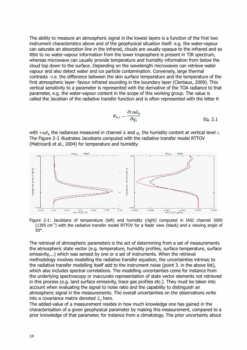
The ability to measure an atmospheric signal in the lowest layers is a function of the first two instrument characteristics above and of the geophysical situation itself: e.g. the water-vapour can saturate an absorption line in the infrared, clouds are usually opaque to the infrared and so little to no water-vapour information from the lower troposphere is present in TIR spectrum, whereas microwave can usually provide temperature and humidity information from below the cloud top down to the surface. Depending on the wavelength microwaves can retrieve water vapour and also detect water and ice particle contamination. Conversely, large thermal contrasts –i.e. the difference between the skin surface temperature and the temperature of the first atmospheric layer- favour infrared sounding in the boundary layer (Clerbaux, 2009). This vertical sensitivity to a parameter is represented with the derivative of the TOA radiance to that parameter, e.g. the water-vapour content in the scope of this working group. The value is called the Jacobian of the radiative transfer function and is often represented with the letter K

Eq. 2.1

with the radiances measured in channel and the humidity content at vertical level . The Figure 2-1 illustrates Jacobians computed with the radiative transfer model RTTOV (Matricardi et al., 2004) for temperature and humidity.

Figure 2-1: Jacobians of temperature (left) and humidity (right) computed in IASI channel 3000

(1395 cm-1) with the radiative transfer model RTTOV for a Nadir view (black) and a viewing angle of 50°.

The retrieval of atmospheric parameters is the act of determining from a set of measurements the atmospheric state vector (e.g. temperature, humidity profiles, surface temperature, surface emissivity,...) which was sensed by one or a set of instruments. When the retrieval methodology involves modelling the radiative transfer equation, the uncertainties intrinsic to the radiative transfer modelling itself add to the instrument noise (point 3. in the above list), which also includes spectral correlations. The modelling uncertainties come for instance from the underlying spectroscopy or inaccurate representation of state vector elements not retrieved in this process (e.g. land surface emissivity, trace gas profiles etc.). They must be taken into account when evaluating the signal to noise ratio and the capability to distinguish an atmospheric signal in the measurements. The overall uncertainties on the observations write into a covariance matrix denoted here. The added-value of a measurement resides in how much knowledge one has gained in the characterisation of a given geophysical parameter by making this measurement, compared to a prior knowledge of that parameter, for instance from a climatology. The prior uncertainty about

19

a parameter is given by its variance around its a priori value –before the measurement is made- and the covariance with other parameters –e.g. variance of the humidity at a given level and covariance with humidity in the rest of the profile-. It is here denoted . The information content of a measurement is conveniently computed with the innovation matrix , (Rodgers, 2000), which combines the theoretical vertical sensitivity of a measurement to a given parameter for a given instrument, K; the uncertainty in distinguishing and reproducing an observation, ; and the uncertainty on the prior knowledge of the geophysical situation, . Eq. 2.2

The number of degrees of freedom for signal (DoFS), or independent pieces of information, one will evaluate from measurements is hence dependent on the assumptions made on the observation and a priori error covariance matrices. Underestimating the measurement errors (e.g. by ignoring the radiative transfer modelling uncertainties) will numerically blow the expected information content and artificially raise the DoFS. Conversely, underestimating the uncertainties on the prior knowledge will result in underestimating the information extracted from the measurements. The vertical sensitivity of a retrieval is characterised by a quantity called the averaging kernel, A. It explains how much a retrieved parameter, e.g. the humidity at 500 hPa, is effectively sensitive to true variations of that parameter.

Eq. 2.3

where and are the retrieved and true quantities, respectively. It can further decompose into:

Eq. 2.4

where is the radiative transfer Jacobian as introduced before and is the gain function, related to the retrieval operator. can be seen as the generalised inverse of . In an ideal world, the averaging kernel function is a Dirac, meaning that the retrieved quantity is only sensitive to the related true quantity, with infinite vertical resolution. In reality, because of the instrument characteristics introduced above and because of the uncertainties inherent to the retrieval method, the retrieved quantity at a given vertical level is actually a weighted summation of contributions from adjacent and sometimes distant levels. Typical averaging kernels for temperature and water-vapour are provided in Figure 2-2. The colour encoding relates to the altitude of the sought retrieved parameter, from red next to the surface to dark blue in the stratosphere.

20

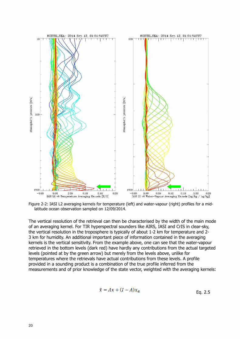
Figure 2-2: IASI L2 averaging kernels for temperature (left) and water-vapour (right) profiles for a mid-

latitude ocean observation sampled on 12/09/2014.

The vertical resolution of the retrieval can then be characterised by the width of the main mode of an averaging kernel. For TIR hyperspectral sounders like AIRS, IASI and CrIS in clear-sky, the vertical resolution in the troposphere is typically of about 1-2 km for temperature and 2-3 km for humidity. An additional important piece of information contained in the averaging kernels is the vertical sensitivity. From the example above, one can see that the water-vapour retrieved in the bottom levels (dark red) have hardly any contributions from the actual targeted levels (pointed at by the green arrow) but merely from the levels above, unlike for temperatures where the retrievals have actual contributions from these levels. A profile provided in a sounding product is a combination of the true profile inferred from the measurements and of prior knowledge of the state vector, weighted with the averaging kernels:

Eq. 2.5

21

and are the retrieved and true profiles, respectively; is the a priori profile; is the identity matrix and is the averaging kernels. Where there is no information extracted from the measurements (averaging kernels close to 0), the retrieved quantities provided in the sounding products actually come from the prior knowledge. The vertical sampling (i.e. number of levels) in satellite sounding products is usually much higher (typically ~100 levels) than the actual number of independent vertical pieces of information in this product. The latter is related to the number of degrees of freedom in that product and can be evaluated by the trace of the averaging kernels (Rodgers, 2000). For hyperspectral IR sounders, there are usually in clear-sky 5 to 9 independent pieces for humidity and 8 to 12 for temperature. Because they characterise the vertical resolution and sensitivity of the satellite sounding products, the averaging kernels are important information which should be provided together with a sounding product to allow proper utilisation for a given application. Also important is the provision of the a priori state vector and the associated error covariance matrix, to understand what in the final product came from the measurements and what came from the a priori. For validation purposes, for instance, the reference profiles can be smoothed by convolution with the averaging kernel to assess the satellite products at their intrinsic vertical resolution. Also, in order to validate the information retrieved from the measurement, the prior information combined in the satellite products can be subtracted before comparison to the reference profile, as nicely exemplified in the didactic paper by (Illingworth, 2010) with carbon monoxide and in (Pougatchev, 2009) for water vapour.

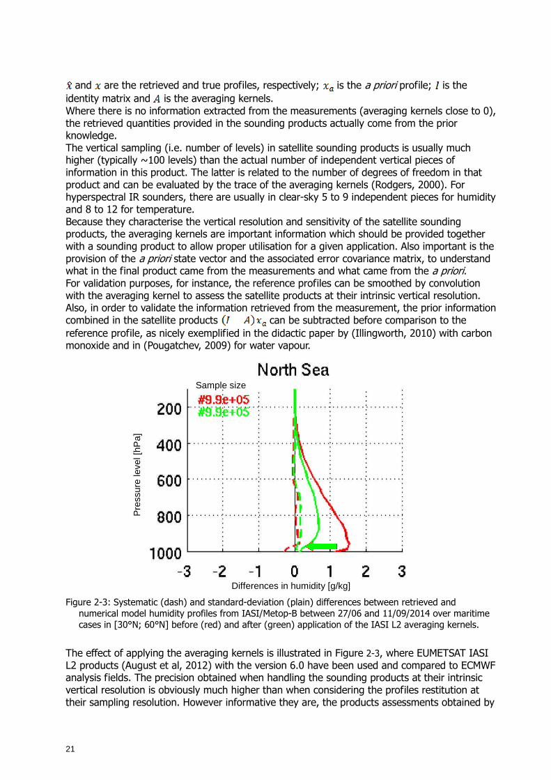
Figure 2-3: Systematic (dash) and standard-deviation (plain) differences between retrieved and

numerical model humidity profiles from IASI/Metop-B between 27/06 and 11/09/2014 over maritime cases in [30°N; 60°N] before (red) and after (green) application of the IASI L2 averaging kernels.

The effect of applying the averaging kernels is illustrated in Figure 2-3, where EUMETSAT IASI L2 products (August et al, 2012) with the version 6.0 have been used and compared to ECMWF analysis fields. The precision obtained when handling the sounding products at their intrinsic vertical resolution is obviously much higher than when considering the profiles restitution at their sampling resolution. However informative they are, the products assessments obtained by

Differences in humidity [g/kg]

Pre

ssur

e le

vel [

hPa]

Sample size

22

application of the averaging kernels must be handled with great care. In the example above one could easily misinterpret the precision characterised in the bottom layers, where the standard deviation drops close to zero (green arrow in Figure 2-3). It does not mean that the precision is infinite but only translates the fact that the retrieval was insensitive to that portion of the atmosphere as highlighted with the green arrow in Figure 2-2. Consequently the product schematically only contains prior information for these levels, hence and: Eq. 2.6

where is the reference profile used to assess the satellite product.

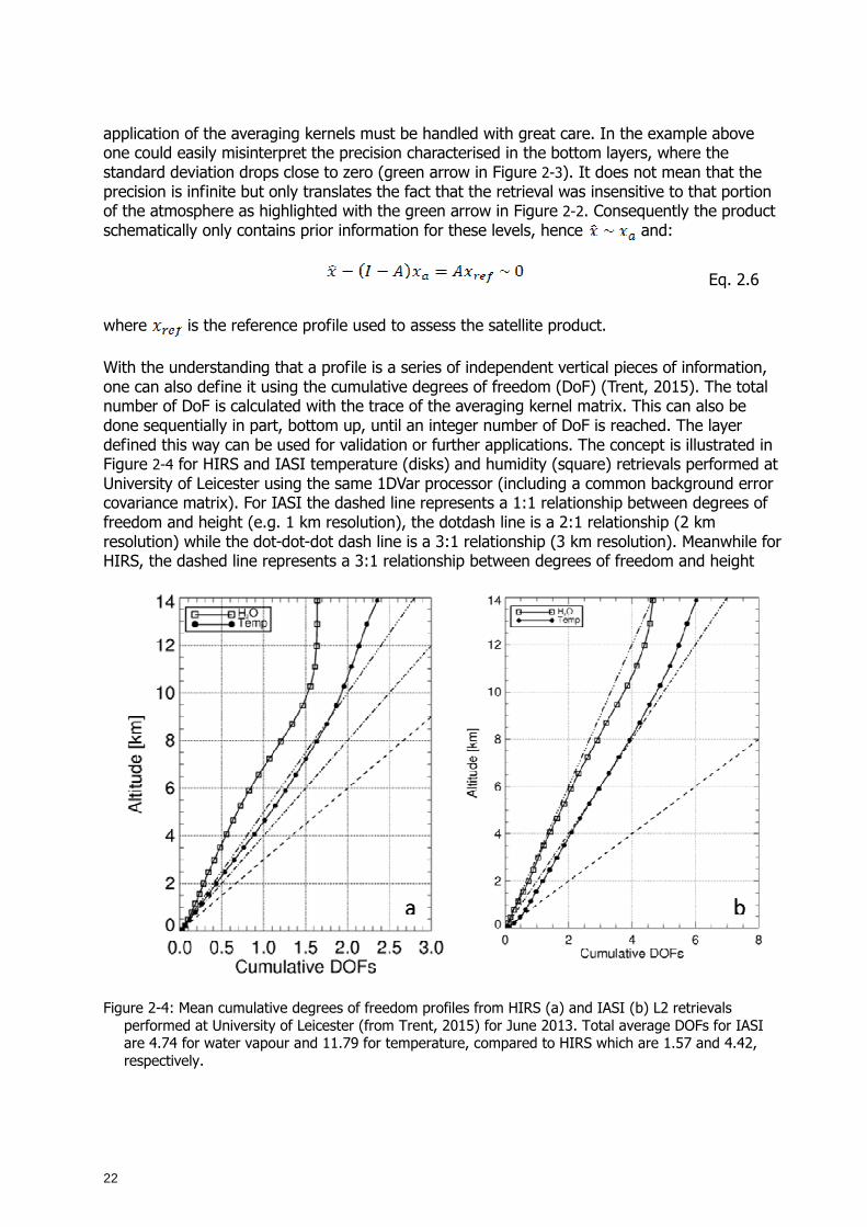
With the understanding that a profile is a series of independent vertical pieces of information, one can also define it using the cumulative degrees of freedom (DoF) (Trent, 2015). The total number of DoF is calculated with the trace of the averaging kernel matrix. This can also be done sequentially in part, bottom up, until an integer number of DoF is reached. The layer defined this way can be used for validation or further applications. The concept is illustrated in Figure 2-4 for HIRS and IASI temperature (disks) and humidity (square) retrievals performed at University of Leicester using the same 1DVar processor (including a common background error covariance matrix). For IASI the dashed line represents a 1:1 relationship between degrees of freedom and height (e.g. 1 km resolution), the dotdash line is a 2:1 relationship (2 km resolution) while the dot-dot-dot dash line is a 3:1 relationship (3 km resolution). Meanwhile for HIRS, the dashed line represents a 3:1 relationship between degrees of freedom and height

Figure 2-4: Mean cumulative degrees of freedom profiles from HIRS (a) and IASI (b) L2 retrievals

performed at University of Leicester (from Trent, 2015) for June 2013. Total average DOFs for IASI are 4.74 for water vapour and 11.79 for temperature, compared to HIRS which are 1.57 and 4.42, respectively.

23

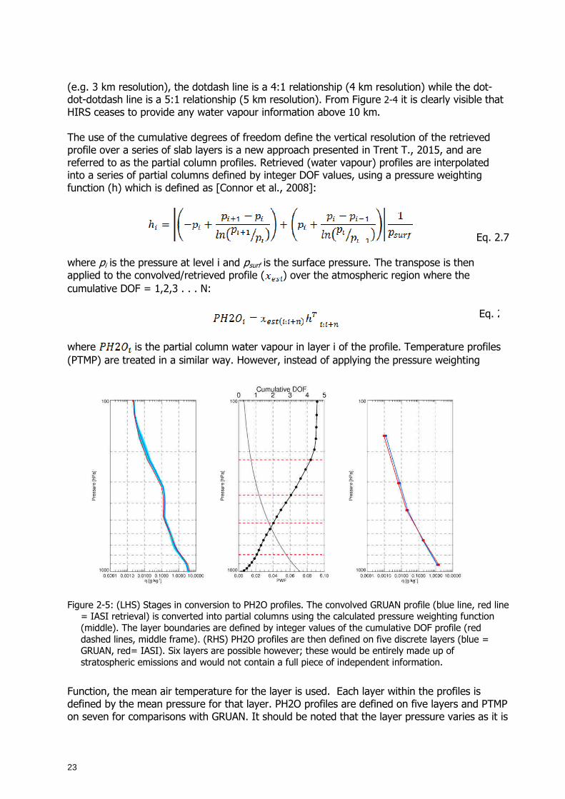
(e.g. 3 km resolution), the dotdash line is a 4:1 relationship (4 km resolution) while the dot-dot-dotdash line is a 5:1 relationship (5 km resolution). From Figure 2-4 it is clearly visible that HIRS ceases to provide any water vapour information above 10 km. The use of the cumulative degrees of freedom define the vertical resolution of the retrieved profile over a series of slab layers is a new approach presented in Trent T., 2015, and are referred to as the partial column profiles. Retrieved (water vapour) profiles are interpolated into a series of partial columns defined by integer DOF values, using a pressure weighting function (h) which is defined as [Connor et al., 2008]:

Eq. 2.7 where pi is the pressure at level i and psurf is the surface pressure. The transpose is then applied to the convolved/retrieved profile ( ) over the atmospheric region where the cumulative DOF = 1,2,3 . . . N:

Eq. 2

where is the partial column water vapour in layer i of the profile. Temperature profiles (PTMP) are treated in a similar way. However, instead of applying the pressure weighting

Figure 2-5: (LHS) Stages in conversion to PH2O profiles. The convolved GRUAN profile (blue line, red line

= IASI retrieval) is converted into partial columns using the calculated pressure weighting function (middle). The layer boundaries are defined by integer values of the cumulative DOF profile (red dashed lines, middle frame). (RHS) PH2O profiles are then defined on five discrete layers (blue = GRUAN, red= IASI). Six layers are possible however; these would be entirely made up of stratospheric emissions and would not contain a full piece of independent information.

Function, the mean air temperature for the layer is used. Each layer within the profiles is defined by the mean pressure for that layer. PH2O profiles are defined on five layers and PTMP on seven for comparisons with GRUAN. It should be noted that the layer pressure varies as it is

24

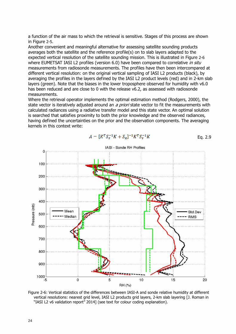
a function of the air mass to which the retrieval is sensitive. Stages of this process are shown in Figure 2-5. Another convenient and meaningful alternative for assessing satellite sounding products averages both the satellite and the reference profile(s) on to slab layers adapted to the expected vertical resolution of the satellite sounding mission. This is illustrated in Figure 2-6 where EUMETSAT IASI L2 profiles (version 6.0) have been compared to correlative in situ measurements from radiosonde measurements. The profiles have then been intercompared at different vertical resolution: on the original vertical sampling of IASI L2 products (black), by averaging the profiles in the layers defined by the IASI L2 product levels (red) and in 2-km slab layers (green). Note that the biases in the lower troposphere observed for humidity with v6.0 has been reduced and are close to 0 with the release v6.2, as assessed with radiosonde measurements. Where the retrieval operator implements the optimal estimation method (Rodgers, 2000), the state vector is iteratively adjusted around an a priori state vector to fit the measurements with calculated radiances using a radiative transfer model and this state vector. An optimal solution is searched that satisfies proximity to both the prior knowledge and the observed radiances, having defined the uncertainties on the prior and the observation components. The averaging kernels in this context write: Eq. 2.9

Figure 2-6: Vertical statistics of the differences between IASI-A and sonde relative humidity at different

vertical resolutions: nearest grid level, IASI L2 products grid layers, 2-km slab layering [J. Roman in “IASI L2 v6 validation report” 2014] (see text for colour coding explanation).

25

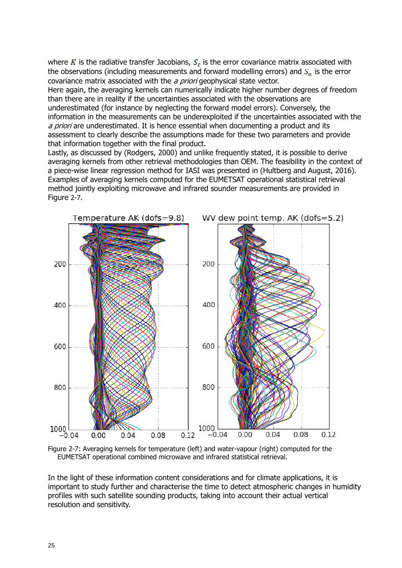
where is the radiative transfer Jacobians, is the error covariance matrix associated with the observations (including measurements and forward modelling errors) and is the error covariance matrix associated with the a priori geophysical state vector. Here again, the averaging kernels can numerically indicate higher number degrees of freedom than there are in reality if the uncertainties associated with the observations are underestimated (for instance by neglecting the forward model errors). Conversely, the information in the measurements can be underexploited if the uncertainties associated with the a priori are underestimated. It is hence essential when documenting a product and its assessment to clearly describe the assumptions made for these two parameters and provide that information together with the final product. Lastly, as discussed by (Rodgers, 2000) and unlike frequently stated, it is possible to derive averaging kernels from other retrieval methodologies than OEM. The feasibility in the context of a piece-wise linear regression method for IASI was presented in (Hultberg and August, 2016). Examples of averaging kernels computed for the EUMETSAT operational statistical retrieval method jointly exploiting microwave and infrared sounder measurements are provided in Figure 2-7.

Figure 2-7: Averaging kernels for temperature (left) and water-vapour (right) computed for the

EUMETSAT operational combined microwave and infrared statistical retrieval.

In the light of these information content considerations and for climate applications, it is important to study further and characterise the time to detect atmospheric changes in humidity profiles with such satellite sounding products, taking into account their actual vertical resolution and sensitivity.

26

3 Data records It follows a general disussion of available satellite sensors, sources of uncertainties in the

retrieval of information on water vapour, an overview of available data records and a general discussion of available ground-based and in-situ data records. Sections 3.1 and 3.3 are largely based on Schröder et al. (2017a).

3.1 Overview on available satellite sensors

J. Forsythe (Colorado State U.), A. Gambacorta (NOAA), R. Kursinski (SSE), M. Schröder (DWD)

In this section we provide background information on the wide variety of sensors that measure atmospheric water vapour. Only sensors that have a greater than 10-year record and cover continental to global scale regions are discussed. These are the types of sensors used to create global climate data records of water vapour.

Water vapour sensors are deployed on low-earth orbiting and geostationary satellites, and are available from several types of surface measurements. Polar-orbiting sensors give global coverage with one day-time (at a particular local time) and one night-time overpass (12 hours later). Geostationary satellites are placed at particular longitudes along the equator and provide useful data up to about 60° of latitude. Since the 1980’s upper tropospheric water vapour has been sensed from geostationary measurements around the 6.7 µm water vapour absorption band. Geostationary sensors allow high temporal sampling of water vapour, typically a few times per hour. Instruments classified as sounders carry several channels distributed about a water vapour absorption line to retrieve the vertical profile of water vapour. Instruments classified as imagers might also have channels clustered about an absorption line, but the primary purpose of an imager is to sense the surface or cloud tops. Imagers are generally restricted to only retrieving TCWV.

The term “profile” usually implies the water vapour amount (mixing ratio) on a given pressure level, such as those measured by a radiosonde. “Profile” can also refer to the retrieval of bulk layers in the atmosphere. Satellite sounding instruments respond to radiation from a great depth of the atmosphere as depicted by the instrument weighting function, so the retrieval of atmospheric layers is the natural unit. These layers might be interpolated to pressure levels to compare with, for instance, a radiosonde or a model, but users should remain aware of the broad vertical depth nominally sampled by satellite sounders.

Rather than focus on a chronological listing of sensors used for water vapour climate data records, this section approaches the overview of sensors from the standpoint of where and what they sample, and the pros and cons of each sensor from a user perspective. Chronological listings are readily available, for instance in Kämpfer (2012; Figure 9.1). A recent overview on sensors and retrieval techniques is also provided by Wulfmeyer et al. (2015). The information provided here is a snapshot in 2015, but radiance records and sensor intercalibration continue to progress, and algorithm improvements can expand the yield and performance of remote retrievals of water vapour. This is not meant to be an exhaustive list, but serves to orient the climate user to the major sensors supporting the water vapour climate data record and their sampling biases. Sensors based on limb sounding techniques that focus on the upper atmosphere are not considered in this report.

27

3.1.1 Resources to track sensor availability

There are a wide variety of water vapour sensors currently operating, and for climate research the sensors change and vary through time. Understanding which sensors were operating at any given time period is a major endeavour. The World Meteorological Organization has created an online tool which makes this task much more feasible. The Observing Systems Capability Analysis and Review Tool (OSCAR) is maintained at http://www.wmo-sat.info/oscar/. This tool allows the user to sort results by sensor type, agency, and atmospheric and surface variables. Time series charts of instrument function can be created. Launch and end of mission life dates are tabulated. Relevance results are generated, but should not be solely relied upon as relevance in the climate sense is a complex question and depends upon sampling limitations and period of performance as well as instrument capability.

3.1.2 Satellite Sensors

3.1.2.1 Passive Microwave Sensors

Passive microwave sensors are typically classified as imagers (channelization focused towards observing the surface) and sounders with channels designed to profile either the temperature or water vapour profile in broad layers. Some instrument names indicate the principal mission of the sensor, e.g. the Special Sensor Microwave Imager (SSM/I) or the Advanced Microwave Sounding Unit (AMSU). Regardless of the classification of the sensor, both imagers and sounders allow water vapour retrievals in clear and cloudy skies, but not in the presence of strong scattering by hydrometeors like during heavy precipitation events.

The passive microwave radiance record, both from imagers and sounders with either a conical or cross-track scan pattern and a few non-scanning, nadir-looking instruments such as the TOPEX Microwave radiometer (TMI) or the ESA’s MicroWave Radiometer (MWR), has exhibited good overlap and continuity since the early 1990’s to the present. The primary spectral bands represented in the climate record are radiances at 19, 22, 37, 50-60, 85-90, and 183 GHz. Many critical climate records are backed by these measurements such as mean tropospheric and stratospheric temperature, sea ice coverage, ocean winds, and precipitation. This record will continue with recent and future sensors such as AMSR-2 on GCOM-W, GMI on GPM, DMSP F19 and F20, ATMS on JPSS, SAPHIR on Megha-Tropiques and the MWI instrument on MetOp-SG, which is planned to measure until ~2040. Intercalibration efforts among the sensors (e.g. Sapiano et al. 2013 and Fennig et al. 2015) yield to fundamental climate data records that can be used to remove time-dependent changes in the radiance record.

a) Imagers

1987 saw the launch of the first SSM/I instrument, a sensor that, while having no official climate mission, has had a profound impact on global water vapour records. The water vapour absorption line at 22 GHz is a key component of these TCWV retrievals, other window channels compensating for cloud and surface roughness effects. Widely used climate data records (e.g. RSS products, HOAPS, NVAP-M), begin in 1988, due to the ocean coverage afforded by the SSM/I and its successor the SSMIS.

Conical scanning microwave imagers are typically configured at an earth incidence angle of about 53 degrees. They have the advantage of constant spatial resolution across the scan, and constant sensitivity to the atmosphere via the same geometric path length. Microwave surface

28

emissivity over land and ocean is a function of incidence angle, so in principal conical scanners eliminate this variable from atmospheric retrievals. Cross-track scanners have changing spatial resolution which is highest at near-nadir views and grows into larger fields-of-view at the outer edge of the scan. They have a minimal atmospheric path length at nadir.

TCWV from passive microwave imagers has historically only been retrieved over the ice-free oceans, and it is commonly stated that passive microwave retrievals work over ocean only. This is due to complex and variable land surface emissivity that changes on short timescales due to surface wetness, vegetation state, and soil properties. There have been efforts to use passive MW for water vapour retrievals over land. The barrier to passive microwave retrievals over land is beginning to fall, at least for operational weather users, as evidenced for instance by the NOAA MIRS sounding system (Boukabara et al. 2011; Forsythe et al. 2015). This record requires further investigation for climate uses. Du et al. (2015) demonstrate an AMSR-2 algorithm to retrieve TCWV over land. For the water vapour climate record, it is most correct to say that passive microwave TCWV has not yet been demonstrated over land, but there is some possibility of this advance in the coming years.

b) Sounders

Passive microwave sounders depend on the water vapour absorption line at 183.31 GHz

to profile water vapour. Historically most water vapour and temperature sounding instruments have been cross-track scanning, and SSMIS is a newer exception. These microwave sounders are often collocated with a companion infrared sounder. Examples are the AIRS instrument onboard the NASA Aqua spacecraft, IASI onboard the Metop spacecraft, and the CrIS instrument on the Suomi-NPP spacecraft. The hyperspectral AIRS, IASI, and CrIS instruments are teamed with companion microwave temperature and moisture sounding instruments, AMSU-A/B or MHS and ATMS respectively. This provides some capability for sounding in cloudy and partly cloudy atmospheres, as the microwave instruments, while having less vertical resolution than the hyperspectral infrared sounders, help constrain the temperature and moisture profile retrieval (e.g. Li et al. 2000, Kahn et al. 2014). Intercalibration efforts for the 183 GHz radiance record continue to move forward (e.g. John et al. 2012 and Chung et al. 2013), but this record that dates back to the early 1990’s has not been fully explored for climate data records.

3.1.2.2 Infrared Sensors

a) Sounders

Infrared sounding sensors constitute the longest satellite record of water vapour profiling and sounding instruments. A key distinction between infrared sensors for water vapour retrievals is between broadband (HIRS, GOES Sounder, MSG SEVIRI instruments) and hyperspectral (AIRS, IASI, CrIS) instruments. The broadband sensors constitute a longer time series (versions of the HIRS instrument span the time back to the early 1980’s), while the hyperspectral instruments allow retrievals with more vertical information and improved uncertainty. The hyperspectral climate record begins with AIRS in 2002, and is augmented by the IASI instrument onboard the Metop-A and –B spacecrafts launched in 2006 and 2012 respectively. The CrIS instrument onboard the Suomi-NPP spacecraft launched in 2011 continues the hyperspectral sounding record. A third IASI instrument is due for launch end of 2018 onboard Metop-C, which will extend the IASI mission and the associated sounding products from 2006 to beyond 2023.

Infrared-only retrievals of TCWV and water vapour profile are retrieved under clear sky

29

conditions only. The combination with passive microwave sounders improves the range of sky conditions in which retrievals are possible. UTH (also referred to as FTH) can be retrieved in clear skies and when cloud tops are close to the surface (e.g., Brogniez et al. 2006). Intercalibration of intersatellite differences within the HIRS record is still continuing (e.g. Shi et al., 2008). There are intersensor differences in the spatial placement of the 20 channels on HIRS, most impactful is the switch of channel 10 from 8.6 µm to 12.5 µm on the HIRS model 3 and 4 sensors beginning with NOAA-15 in 1998.

Yue et al. (2013) characterized the sampling biases of AIRS soundings in the presence of different cloud classes, and deep convection and nimbostratus have the largest impacts. These impacts and biases affect all infrared-based water vapour retrieval systems. While land surface emissivity is much more uniform and less time-varying in the infrared than at microwave wavelengths, infrared land surface emissivity does vary (Seemann et al. 2008) and can be problematic for infrared retrievals, especially over desert surfaces.

b) Ultraviolet/Visible/Near-Infrared Imagers

A daylight retrieval using two channels at 0.885 µm (window) and 0.9 µm (water vapour

absorption) has been demonstrated from the MERIS instrument (Lindstrot et al. 2014). The retrieval is limited to the daylight portion of the swath, as differential solar reflectance is the signal for this retrieval. These types of retrievals have the benefit of high spatial resolution (~ 1 km), but the TCWV retrieval is limited to clear skies to sense the entire column to Earth’s surface. The MERIS instrument was launched in 2002, while MODIS onboard the Terra spacecraft begins in 1999, and is complemented by the MODIS onboard the Aqua spacecraft which was launched in 2002. Both MODIS instruments continue to function in 2015, so further extension of the TCWV record from these sensors is feasible. Retrievals from MERIS and MODIS complement passive microwave TCWV retrievals because they perform best over land and have reduced quality over oceans.

UV/VIS spectrometers such as the Global Ozone Monitoring Experiment (GOME and GOME-2) and Scanning Imaging Absorption Spectrometer for Atmospheric Chartography (SCIAMACHY) allow for the retrieval of total column water vapour over land and ocean surfaces under daylight and clear sky conditions. The resolution is between 320 km x 40 km and 80 km x 40 km, with cloud handling being a major challenge.

Future European missions such as GMES Sentinel 3, Sentinel 4, Sentinel 5 precursor and Sentinel 5 will carry UV/VIS/NIR spectrometers, in particular OLCI (Ocean Land Colour Instrument on Sentinel 3), which will extend the total column water vapour record.

3.1.2.3 Limb Sounding

Limb sounding is the technique of sounding various layers of the atmosphere by observation along a tangent ray that does not intersect Earth’s surface. The extinction of a source of radiation, either the sun or in the case of GPS radio occultation (GPS-RO) a transmitting spacecraft is measured at various layers of the atmosphere. This technique has been especially important to study stratospheric water vapour. A separate WCRP effort called Stratosphere-troposphere Processes and their Role in Climate (SPARC; http://www.sparc-climate.org/) is devoted to this topic while G-VAP focuses on tropospheric water vapour. Moisture profiles in the highest levels of the troposphere, centered on 215 hPa, have been derived and the satellite record begins in the earlyy1990s. The HALOE instrument on the UARS spacecraft, SAGE II and the MLS microwave sensor constitute the core of this record. GPS-RO is particularly relevant in the context of climate and is discussed below. Limb sounding using

30

the sun is limited by an inability to retrieve water vapour near the surface, and also by coarse horizontal resolution on a scale of one hundred kilometres along the ray.

3.1.2.4 GPS Radio Occultation

GNSS radio occultation (RO) measurements profile atmospheric refractivity with globally-distributed, all-weather sampling from which tropospheric water vapour is derived. The water vapour information is isolated by combining the GNSS RO refractivity profile with temperature information from NWP analyses interpolated to the time and location of the RO profile. GPS-RO missions began with the prototype GPS-MET mission from April 1995 – Feb. 1997. Global Navigation Satellite System Receiver for Atmospheric Sounding (GRAS) is flying onboard Metop-A and Metop-B since 2007 and 2012, respectively. The CHAMP mission flew from 2000 to 2009 and provided about 250 occultations per day. A significant increase in RO sampling density to 2,000 or more occultation profiles per day began with the launch of the 6-satellite COSMIC mission in April 2006. The COSMIC satellites orbits were also spread in longitude to provide full sampling of the diurnal cycle. Occultation profiles from the GPS-RO receiver on CHAMP satellites only penetrate into the upper to middle troposphere, which has limited their utility for tropospheric water vapour. This is because it uses closed loop tracking of the GPS signals. The COSMIC and the GRAS GPS-RO receivers use an “open loop” tracking capability and a raw-sampling mode. These enabled a far higher percentage of the occultation profiles to extend to within 1 km of the surface, making them far more useful for characterizing tropospheric water vapour.

From the GNSS RO receiver phase measurements during each occultation, the bending of the signal path due to its passage through the atmosphere is determined. The bending angle profile is then inverted to a profile of the index of refraction that caused the bending. The dual frequency GNSS signals are used to isolate and remove the effects of the ionosphere.

The atmospheric index of refraction is due to the combined effects of the dry gas and the water vapour. The water vapour contribution to the measured refractivity is typically isolated using one of two approaches. The first is a variational technique used in NWP assimilation systems where estimates of the water vapour, temperature and pressure structures from the forecast and their associated error covariances are combined with the GPS occultation bending angle or refractivity profile and its error covariance to achieve a new best estimate, in a least squares sense (e.g. Healy and Eyre, 2010). The second approach, referred to as the “Direct” method, estimates the dry part of the refractivity from the analysis temperature that is then subtracted from the GPS-measured total refractivity to obtain the wet part of the refractivity. The latter is then scaled to obtain the water vapour. Both methods rely on the analysis temperatures that are a combination of observations and of the NWP model. The advantage of the Direct method is that it does not rely on estimates of water vapour from models, forecasts or climatologies and is therefore unaffected by biases in those estimates.

GNSS RO has very high vertical resolution for a satellite system (about 200 m) and relatively coarse horizontal resolution of about 100 km (Kursinski et al., 1997, eqn. 13) because it is a limb sounder. The altitude range of GPS-RO individual profiles of water vapour extends from the surface to about the 240 K-temperature level in the troposphere with zonal means extending somewhat higher. As a result, at mid to high latitudes, GPS-RO water vapour profiles extend to higher altitudes in the summer hemisphere. At low latitudes, Kursinski and Gebhardt (2014) determined the 1-sigma uncertainty in specific humidity to be 0.14 g/kg at 350 mb and 0.39 g/kg at 725 mb and estimated the magnitude of the bias to be no more than 0.03 g/kg.

GPS-RO’s ability to routinely penetrate through clouds combined with its insensitivity to surface emissivity eliminates sampling biases that limit other satellite measurement systems. A caveat

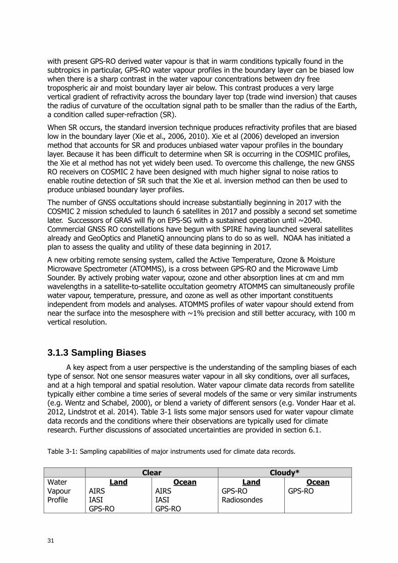
31

with present GPS-RO derived water vapour is that in warm conditions typically found in the subtropics in particular, GPS-RO water vapour profiles in the boundary layer can be biased low when there is a sharp contrast in the water vapour concentrations between dry free tropospheric air and moist boundary layer air below. This contrast produces a very large vertical gradient of refractivity across the boundary layer top (trade wind inversion) that causes the radius of curvature of the occultation signal path to be smaller than the radius of the Earth, a condition called super-refraction (SR).

When SR occurs, the standard inversion technique produces refractivity profiles that are biased low in the boundary layer (Xie et al., 2006, 2010). Xie et al (2006) developed an inversion method that accounts for SR and produces unbiased water vapour profiles in the boundary layer. Because it has been difficult to determine when SR is occurring in the COSMIC profiles, the Xie et al method has not yet widely been used. To overcome this challenge, the new GNSS RO receivers on COSMIC 2 have been designed with much higher signal to noise ratios to enable routine detection of SR such that the Xie et al. inversion method can then be used to produce unbiased boundary layer profiles.

The number of GNSS occultations should increase substantially beginning in 2017 with the COSMIC 2 mission scheduled to launch 6 satellites in 2017 and possibly a second set sometime later. Successors of GRAS will fly on EPS-SG with a sustained operation until ~2040. Commercial GNSS RO constellations have begun with SPIRE having launched several satellites already and GeoOptics and PlanetiQ announcing plans to do so as well. NOAA has initiated a plan to assess the quality and utility of these data beginning in 2017.

A new orbiting remote sensing system, called the Active Temperature, Ozone & Moisture Microwave Spectrometer (ATOMMS), is a cross between GPS-RO and the Microwave Limb Sounder. By actively probing water vapour, ozone and other absorption lines at cm and mm wavelengths in a satellite-to-satellite occultation geometry ATOMMS can simultaneously profile water vapour, temperature, pressure, and ozone as well as other important constituents independent from models and analyses. ATOMMS profiles of water vapour should extend from near the surface into the mesosphere with ~1% precision and still better accuracy, with 100 m vertical resolution.

3.1.3 Sampling Biases

A key aspect from a user perspective is the understanding of the sampling biases of each type of sensor. Not one sensor measures water vapour in all sky conditions, over all surfaces, and at a high temporal and spatial resolution. Water vapour climate data records from satellite typically either combine a time series of several models of the same or very similar instruments (e.g. Wentz and Schabel, 2000), or blend a variety of different sensors (e.g. Vonder Haar et al. 2012, Lindstrot et al. 2014). Table 3-1 lists some major sensors used for water vapour climate data records and the conditions where their observations are typically used for climate research. Further discussions of associated uncertainties are provided in section 6.1.

Table 3-1: Sampling capabilities of major instruments used for climate data records.

Clear Cloudy*

Water Vapour Profile

Land AIRS IASI GPS-RO

Ocean AIRS IASI GPS-RO

Land GPS-RO Radiosondes

Ocean GPS-RO

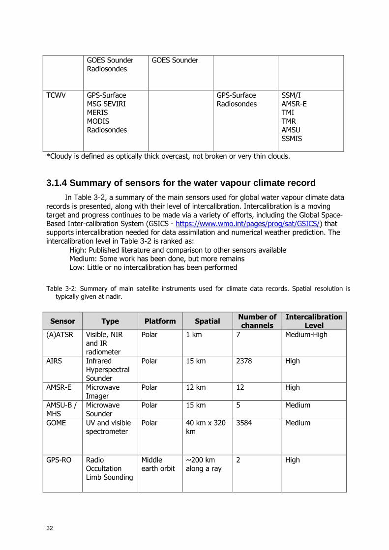
32

GOES Sounder Radiosondes

GOES Sounder

TCWV GPS-Surface MSG SEVIRI MERIS MODIS Radiosondes

GPS-Surface Radiosondes

SSM/I AMSR-E TMI TMR AMSU SSMIS

*Cloudy is defined as optically thick overcast, not broken or very thin clouds.

3.1.4 Summary of sensors for the water vapour clima te record

In Table 3-2, a summary of the main sensors used for global water vapour climate data records is presented, along with their level of intercalibration. Intercalibration is a moving target and progress continues to be made via a variety of efforts, including the Global Space-Based Inter-calibration System (GSICS - https://www.wmo.int/pages/prog/sat/GSICS/) that supports intercalibration needed for data assimilation and numerical weather prediction. The intercalibration level in Table 3-2 is ranked as:

High: Published literature and comparison to other sensors available Medium: Some work has been done, but more remains Low: Little or no intercalibration has been performed

Table 3-2: Summary of main satellite instruments used for climate data records. Spatial resolution is typically given at nadir.

Sensor Type Platform Spatial Number of channels

Intercalibration Level

(A)ATSR Visible, NIR and IR radiometer

Polar 1 km 7 Medium-High

AIRS Infrared Hyperspectral Sounder

Polar 15 km 2378 High

AMSR-E

Microwave Imager

Polar 12 km 12 High

AMSU-B / MHS

Microwave Sounder

Polar 15 km 5 Medium

GOME UV and visible spectrometer

Polar 40 km x 320 km

3584 Medium

GPS-RO

Radio Occultation Limb Sounding

Middle earth orbit

~200 km along a ray

2 High

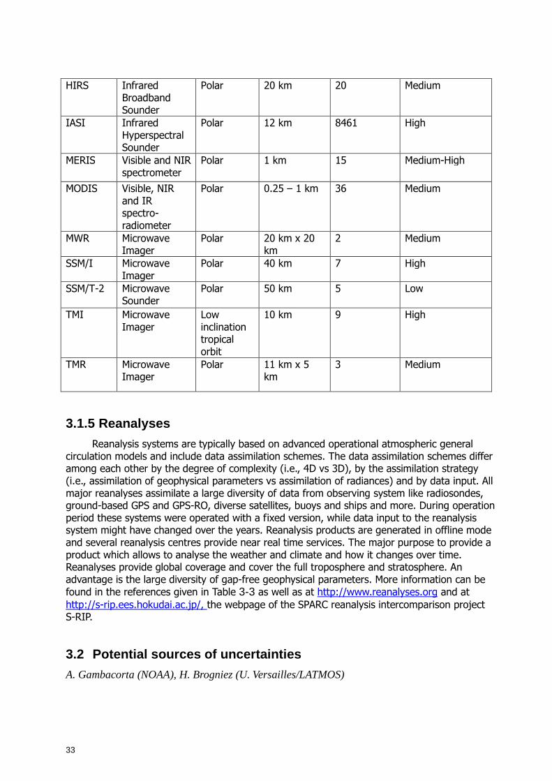
33

HIRS Infrared Broadband Sounder

Polar 20 km 20 Medium

IASI Infrared Hyperspectral Sounder

Polar 12 km 8461 High

MERIS

Visible and NIR spectrometer

Polar 1 km 15 Medium-High

MODIS

Visible, NIR and IR spectro-radiometer

Polar 0.25 – 1 km 36 Medium

MWR Microwave Imager

Polar 20 km x 20 km

2 Medium

SSM/I Microwave Imager

Polar 40 km 7 High

SSM/T-2

Microwave Sounder

Polar 50 km 5 Low

TMI

Microwave Imager

Low inclination tropical orbit

10 km 9 High

TMR

Microwave Imager

Polar 11 km x 5 km

3 Medium

3.1.5 Reanalyses

Reanalysis systems are typically based on advanced operational atmospheric general circulation models and include data assimilation schemes. The data assimilation schemes differ among each other by the degree of complexity (i.e., 4D vs 3D), by the assimilation strategy (i.e., assimilation of geophysical parameters vs assimilation of radiances) and by data input. All major reanalyses assimilate a large diversity of data from observing system like radiosondes, ground-based GPS and GPS-RO, diverse satellites, buoys and ships and more. During operation period these systems were operated with a fixed version, while data input to the reanalysis system might have changed over the years. Reanalysis products are generated in offline mode and several reanalysis centres provide near real time services. The major purpose to provide a product which allows to analyse the weather and climate and how it changes over time. Reanalyses provide global coverage and cover the full troposphere and stratosphere. An advantage is the large diversity of gap-free geophysical parameters. More information can be found in the references given in Table 3-3 as well as at http://www.reanalyses.org and at http://s-rip.ees.hokudai.ac.jp/, the webpage of the SPARC reanalysis intercomparison project S-RIP.

3.2 Potential sources of uncertainties

A. Gambacorta (NOAA), H. Brogniez (U. Versailles/LATMOS)

34

The focus of this section is to provide a general description on the sources of errors in satellite-based retrievals of water vapour. Understanding these sources of uncertainty is central for a climate quality assessment of a water vapour retrieval product. Here the discussion of uncertainties is oriented at GRUAN practices. Following the GRUAN guidelines, the consistency between the retrieval and the truth (or a reference) is obtained by appropriately relating the computed retrieval bias to the combination of three inherent error sources: Xret – Xtru < k [εt

2 + εr

2 + εcoll

2]1/2 Eq. 3.1 where Xret is the actual water vapour retrieval profile, Xtru is the water vapour truth profile. The elements in the parenthesis are respectively the truth error estimate, εt; the retrieval error estimate εr; and the temporal and spatial mismatch between truth and retrieval profile, εcoll. The parameter k is a scaling parameter used to scale the sum of all contributing error estimates with respect to the truth error estimates. It has undergone different definitions with time.

3.2.1 Sources contributing to the reference error e stimate εt

GRUAN standards now request uncertainty estimates for all upper-air parameters on each individual measurement level. All sources of uncertainty in the truth ensemble should be integral part of the truth data record (Miloshevich et al., 2006; Miloshevich et al, 2009; Immler et al, 2010; Nash et al., 2010). The list below outlines the main sources of temperature and water vapour uncertainties. (i) Temperature systematic errors: Some sources of errors are more significant than others, depending on the radiosonde type, and their uncertainty also varies. Overall four main sources have been identified, although not all of them are relevant for a given probe:

• The solar radiative heating of the air in direct contact with the sensor polymer (normally corrected, correction uncertainty is provided).

• Temperature spikes due to patches of warm air coming off the sensor housing and the balloon (also corrected for, correction uncertainty is provided).

• Evaporative cooling of the wetted sensor after exiting a cloud (not corrected because too difficult to evaluate, but is flagged).

• Sensor time lag, induced by the finite response time of the sensor to more or less sharp gradients (sometimes corrected, see Miloshevich et al., 2004, but overall negligible). This results in a smoothing of the profile. (ii) Humidity systematic errors: Three main sources of humidity error have been

identified: • Daytime solar heating of the sensors, thoroughly documented for the Vaisala probes,

which yields to the measured RH near the sensor to be lower than the ambient air. • Sensor time-lag at temperatures below about -40°C, more specifically important above

and below cirrus layers at the tropopause (steep gradients of humidity). • Temperature-dependent calibration correction.

3.2.2 Sources contributing to the retrieval error e stimate, εr

Retrieval error estimates result from the summation of a smoothing and a measurement error.

35

(i) Smoothing errors: Smoothing errors originate from the smoothing effect of the observing system (the combination of measurement and inversion) that operates the measurement on the atmospheric state. The smoothing operator is expressed by the averaging kernel function A (see section 2.5). The retrieval solution, as derived from a traditional optimal estimation approach, can be expressed as a weighted average of the truth profile and the a priori (Xap), the weights being defined by the averaging kernel. Specifically, we can write: Xret = A*Xtru + (I-A)Xap Eq. 3.2 As explained in Rodgers (2000), in an ideal case, the averaging kernel would be a delta function of pressure. Nonetheless, each channel is characterized by a distinctive single peaked but coarse averaging kernel function. The coarse feature provides a simple characterization of the relationship existing between the true state and the retrieval. Analysis of averaging kernels can explain important features of a retrieval algorithm, such as the vertical resolution and effective sensitivity of a retrieval profile and the precise contribution provided by the a-priori to retrieval solution. Therefore, averaging kernels should be an integral part of a profile data record. Thus also the uncertainties of the a priori information and of the averaging kernel impact to the retrieval uncertainty.

(ii) Measurement errors: measurement errors originate from different sources. These are: 1) errors in the forward model relative to the real physics and errors in the parameters used in the forward model; 2) instrument noise and calibration errors; 3) spectrally correlated errors. Measurement errors can be confounded with real atmospheric signal and introduce an error in the final retrieval products. For this reason, all sources of error in the measurements should be evaluated as an integral part of a retrieval product assessment.

3.2.3 Temporal and spatial mismatch error sources

A number of studies have proven that temporal and spatial mismatching existing between the truth and the retrieval can introduce misleading results in a retrieval performance effort (Sun et al., 2013). This is particularly true for water vapour retrievals over land where surface emissivity has high variability in time and space. For instance, it has been shown that up to a 10% RMS increase can be observed per 100 km-mismatch between the location of the reference profile and the retrieval ensemble. Closely matched reference profiles are highly favourable but generally of limited availability. Even then the reference data may not be fully representative of the scene observed by the satellite. In section 6.3 more details and potential ways forward are discussed. Hence, particular attention needs to be paid in this assessment aimed at obtaining a consistent and uniformly collocated ensemble of reference profiles across all satellite data records. Additional sources of uncertainty are given in Kummerow et al. (2011), which is based on output from the first G-VAP workshop and from the work of the GEWEX Aerosol Assessment (http://www.meto.umd.edu/~zli/GAPA/gapa_main.htm). Structural uncertainties are further discussed in section 6.2.

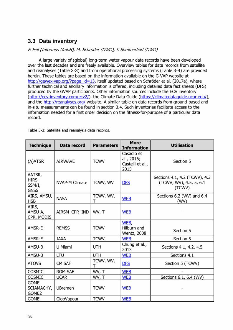
36

3.3 Data inventory

F. Fell (Informus GmbH), M. Schröder (DWD), I. Sommerfeld (DWD)

A large variety of (global) long-term water vapour data records have been developed over the last decades and are freely available. Overview tables for data records from satellite and reanalyses (Table 3-3) and from operational processing systems (Table 3-4) are provided herein. These tables are based on the information available on the G-VAP website at http://gewex-vap.org/?page_id=13, itself updated based on Schröder et al. (2017a), where further technical and ancillary information is offered, including detailed data fact sheets (DFS) produced by the GVAP participants. Other information sources include the ECV inventory (http://ecv-inventory.com/ecv2/), the Climate Data Guide (https://climatedataguide.ucar.edu/), and the http://reanalyses.org/ website. A similar table on data records from ground-based and in-situ measurements can be found in section 3.4. Such inventories facilitate access to the information needed for a first order decision on the fitness-for-purpose of a particular data record.

Table 3-3: Satellite and reanalysis data records.

Technique Data record Parameters More

Information Utilisation

(A)ATSR AIRWAVE TCWV

Casadio et al., 2016; Castelli et al., 2015

Section 5

AATSR, HIRS, SSM/I, GNSS

NVAP-M Climate TCWV, WV DFS Sections 4.1, 4.2 (TCWV), 4.3

(TCWV, WV), 4.5, 5, 6.1 (TCWV)

AIRS, AMSU, HSB

NASA TCWV, WV, T

WEB Sections 6.2 (WV) and 6.4

(WV) AIRS, AMSU-A, CPR, MODIS

AIRSM_CPR_IND WV, T WEB -

AMSR-E REMSS TCWV WEB, Hilburn and Wentz, 2008

Section 5

AMSR-E JAXA TCWV WEB Section 5

AMSU-B U Miami UTH Chung et al., 2013

Sections 4.1, 4.2, 4.5

AMSU-B LTU UTH WEB Sections 4.1

ATOVS CM SAF TCWV, WV, T

DFS Section 5 (TCWV)

COSMIC ROM SAF WV, T WEB - COSMIC UCAR WV, T WEB Sections 6.1, 6.4 (WV) GOME, SCIAMACHY, GOME2

UBremen TCWV WEB -

GOME, GlobVapour TCWV WEB

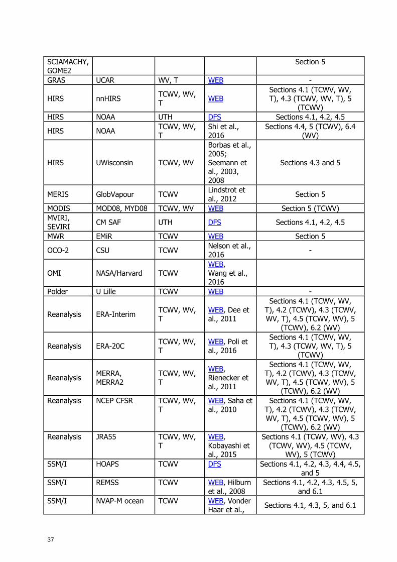
37

SCIAMACHY, GOME2

Section 5

GRAS UCAR WV, T WEB -

HIRS nnHIRS TCWV, WV, T

WEB Sections 4.1 (TCWV, WV, T), 4.3 (TCWV, WV, T), 5

(TCWV) HIRS NOAA UTH DFS Sections 4.1, 4.2, 4.5

HIRS NOAA TCWV, WV, T

Shi et al., 2016

Sections 4.4, 5 (TCWV), 6.4 (WV)

HIRS UWisconsin TCWV, WV

Borbas et al., 2005; Seemann et al., 2003, 2008

Sections 4.3 and 5

MERIS GlobVapour TCWV Lindstrot et al., 2012

Section 5

MODIS MOD08, MYD08 TCWV, WV WEB Section 5 (TCWV) MVIRI, SEVIRI

CM SAF UTH DFS Sections 4.1, 4.2, 4.5

MWR EMiR TCWV WEB Section 5

OCO-2 CSU TCWV Nelson et al., 2016

-

OMI NASA/Harvard TCWV WEB, Wang et al., 2016

Polder U Lille TCWV WEB -

Reanalysis ERA-Interim TCWV, WV, T

WEB, Dee et al., 2011

Sections 4.1 (TCWV, WV, T), 4.2 (TCWV), 4.3 (TCWV, WV, T), 4.5 (TCWV, WV), 5

(TCWV), 6.2 (WV)

Reanalysis ERA-20C TCWV, WV, T

WEB, Poli et al., 2016

Sections 4.1 (TCWV, WV, T), 4.3 (TCWV, WV, T), 5

(TCWV)

Reanalysis MERRA, MERRA2

TCWV, WV, T

WEB, Rienecker et al., 2011

Sections 4.1 (TCWV, WV, T), 4.2 (TCWV), 4.3 (TCWV, WV, T), 4.5 (TCWV, WV), 5

(TCWV), 6.2 (WV) Reanalysis NCEP CFSR TCWV, WV,

T WEB, Saha et al., 2010

Sections 4.1 (TCWV, WV, T), 4.2 (TCWV), 4.3 (TCWV, WV, T), 4.5 (TCWV, WV), 5

(TCWV), 6.2 (WV) Reanalysis JRA55 TCWV, WV,

T WEB, Kobayashi et al., 2015

Sections 4.1 (TCWV, WV), 4.3 (TCWV, WV), 4.5 (TCWV,

WV), 5 (TCWV) SSM/I HOAPS TCWV DFS Sections 4.1, 4.2, 4.3, 4.4, 4.5,

and 5 SSM/I REMSS TCWV WEB, Hilburn

et al., 2008 Sections 4.1, 4.2, 4.3, 4.5, 5,

and 6.1 SSM/I NVAP-M ocean TCWV WEB, Vonder

Haar et al., Sections 4.1, 4.3, 5, and 6.1

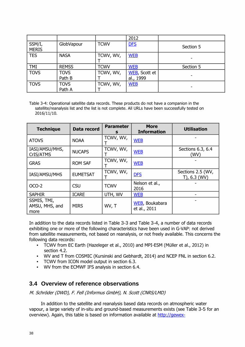
38

2012 SSM/I, MERIS

GlobVapour TCWV DFS Section 5

TES NASA TCWV, WV, T

WEB -

TMI REMSS TCWV WEB Section 5 TOVS TOVS

Path B TCWV, WV, T

WEB, Scott et al., 1999

-

TOVS

TOVS Path A

TCWV, WV, T

WEB -

Table 3-4: Operational satellite data records. These products do not have a companion in the satellite/reanalysis list and the list is not complete. All URLs have been successfully tested on 2016/11/10.

Technique Data record Parameter

s More

Information Utilisation

ATOVS NOAA TCWV, WV, T

WEB -

IASI/AMSU/MHS, CrIS/ATMS

NUCAPS TCWV, WV, T

WEB Sections 6.3, 6.4

(WV)

GRAS ROM SAF TCWV, WV, T

WEB -

IASI/AMSU/MHS EUMETSAT TCWV, WV, T

DFS Sections 2.5 (WV,

T), 6.3 (WV)

OCO-2 CSU TCWV Nelson et al., 2016

-

SAPHIR ICARE UTH, WV WEB - SSMIS, TMI, AMSU, MHS, and more

MIRS WV, T WEB, Boukabara et al., 2011

-

In addition to the data records listed in Table 3-3 and Table 3-4, a number of data records exhibiting one or more of the following characteristics have been used in G-VAP: not derived from satellite measurements, not based on reanalysis, or not freely available. This concerns the following data records:

• TCWV from EC Earth (Hazeleger et al., 2010) and MPI-ESM (Müller et al., 2012) in section 4.2.

• WV and T from COSMIC (Kursinski and Gebhardt, 2014) and NCEP FNL in section 6.2. • TCWV from ICON model output in section 6.3. • WV from the ECMWF IFS analysis in section 6.4.

3.4 Overview of reference observations

M. Schröder (DWD), F. Fell (Informus GmbH), N. Scott (CNRS/LMD)

In addition to the satellite and reanalysis based data records on atmospheric water vapour, a large variety of in-situ and ground-based measurements exists (see Table 3-5 for an overview). Again, this table is based on information available at http://gewex-

39

vap.org/?page_id=13, where further technical and ancillary information is offered, including detailed DFS produced by the GVAP participants.

Table 3-5: Ground-based and in situ data records. All URLs have been successfully tested on 2016/11/10.

Technique Data record Parameters More

Information Utilisation

FPH NOAA WV WEB -

FTIR MUSICA, NDACC

WV WEB, Schneider et al., 2012

-

Ground-based GNSS

UCAR TCWV DFS, WEB, Wang et al., 2007

Sections 3.4 and 6.1

Lidar NDACC WV WEB, Leblanc et al., 2012

-

Lidar ARM TCWV, WV, T WEB - MWR NDACC TCWV, WV WEB - MWR ARM TCWV, WV, T WEB_1, WEB_2,

Cadeddu et al., 2013

-

Radiosonde GRUAN TCWV, WV, T WEB, Dirksen et al., 2014

Sections 2.5, 6.4

Radiosonde IGRA TCWV, WV, T WEB, Durre et al., 2006

-

Radiosonde HomoRS92 TCWV, WV, T Dai et al., 2011 Sections 3.4, 4.1 Radiosonde ARSA TCWV, WV, T WEB Sections 3.4, 4.4

Sun photometer AERONET TCWV WEB, Holben et al., 2001

Section 3.4

In addition to the data records listed in Table 3-5, additional data records have been used which are either not multi-station or not freely available:

• TCWV from ground-based GPS at ARM sites in section 4.3 and WV from radiosondes at ARM site in section 2.5.

• WV from the Characterised Radiosonde Measurements (CRM, Trent et al., 2016) and from AEROSE (Nalli et al., 2013) in section 6.4.

Of particular interest to G-VAP are long-term (at least a decade) multi-station (at least a few tens of stations) ground-based and in-situ data records which ideally have been quality controlled, intercalibrated/homogenised and consistently reprocessed.

Three such radiosonde records constitute a long-term time series of tropospheric water vapour (ARSA, homogenised IGRA, IGRA) from multiple stations. Particularly the water vapour data suffer from measurement biases among others due to changes of the moisture sensors, particularly between nations. Radiosonde water vapour quality is impaired at cold temperatures below -40° C. There have been several efforts to intercalibrate or homogenize the radiosonde record (e.g. Durre et al., 2008; Dai et al., 2011), and progress has been made, particularly for lower tropospheric moisture at temperatures not far below freezing. Radiosondes from the GRUAN network largely fulfil the quality requirements. As the GRUAN is still expanding such data is highly relevant for future climate analysis.

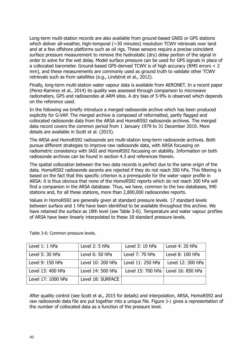
40

Long-term multi-station records are also available from ground-based GNSS or GPS stations which deliver all-weather, high-temporal (~30 minutes) resolution TCWV retrievals over land and at a few offshore platforms such as oil rigs. These sensors require a precise coincident surface pressure measurement to remove the hydrostatic (dry) delay portion of the signal in order to solve for the wet delay. Model surface pressure can be used for GPS signals in place of a collocated barometer. Ground-based GPS-derived TCWV is of high accuracy (RMS errors < 2 mm), and these measurements are commonly used as ground truth to validate other TCWV retrievals such as from satellites (e.g., Lindstrot et al., 2012).

Finally, long-term multi-station water vapour data is available from AERONET. In a recent paper (Perez-Ramirez et al., 2014) its quality was assessed through comparison to microwave radiometers, GPS and radiosondes at ARM sites. A dry bias of 5-9% is observed which depends on the reference used.

In the following we briefly introduce a merged radiosonde archive which has been produced explicitly for G-VAP. The merged archive is composed of reformatted, partly flagged and collocated radiosonde data from the ARSA and HomoRS92 radiosonde archives. The merged data record covers the common period from 1 January 1979 to 31 December 2010. More details are available in Scott et al. (2015).

The ARSA and HomoRS92 radiosonde are multi-station long-term radiosonde archives. Both pursue different strategies to improve raw radiosonde data, with ARSA focussing on radiometric consistency with IASI and HomoRS92 focussing on stability. Information on both radiosonde archives can be found in section 4.3 and references therein.

The spatial collocation between the two data records is perfect due to the same origin of the data. HomoRS92 radiosonde ascents are rejected if they do not reach 300 hPa. This filtering is based on the fact that this specific criterion is a prerequisite for the water vapor profile in ARSA: it is thus obvious that none of the HomoRS92 reports which do not reach 300 hPa will find a companion in the ARSA database. Thus, we have, common to the two databases, 940 stations and, for all these stations, more than 2,800,000 radiosondes reports.

Values in HomoRS92 are generally given at standard pressure levels. 17 standard levels between surface and 1 hPa have been identified to be available throughout this archive. We have retained the surface as 18th level (see Table 3-6). Temperature and water vapour profiles of ARSA have been linearly interpolated to these 18 standard pressure levels.

Table 3-6: Common pressure levels.

Level 1: 1 hPa Level 2: 5 hPa Level 3: 10 hPa Level 4: 20 hPa

Level 5: 30 hPa Level 6: 50 hPa Level 7: 70 hPa Level 8: 100 hPa

Level 9: 150 hPa Level 10: 200 hPa Level 11: 250 hPa Level 12: 300 hPa

Level 13: 400 hPa Level 14: 500 hPa Level 15: 700 hPa Level 16: 850 hPa

Level 17: 1000 hPa Level 18: SURFACE

After quality control (see Scott et al., 2015 for details) and interpolation, ARSA, HomoRS92 and raw radiosonde data file are put together into a unique file. Figure 3-1 gives a representation of the number of collocated data as a function of the pressure level.

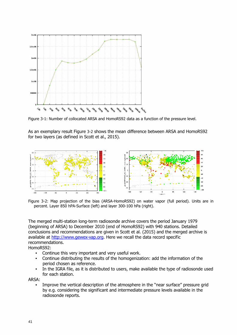
41

Figure 3-1: Number of collocated ARSA and HomoRS92 data as a function of the pressure level.

As an exemplary result Figure 3-2 shows the mean difference between ARSA and HomoRS92 for two layers (as defined in Scott et al., 2015).

Figure 3-2: Map projection of the bias (ARSA-HomoRS92) on water vapor (full period). Units are in percent. Layer 850 hPA-Surface (left) and layer 300-100 hPa (right).

The merged multi-station long-term radiosonde archive covers the period January 1979 (beginning of ARSA) to December 2010 (end of HomoRS92) with 940 stations. Detailed conclusions and recommendations are given in Scott et al. (2015) and the merged archive is available at http://www.gewex-vap.org. Here we recall the data record specific recommendations. HomoRS92:

• Continue this very important and very useful work. • Continue distributing the results of the homogenization: add the information of the

period chosen as reference. • In the IGRA file, as it is distributed to users, make available the type of radiosonde used

for each station. ARSA:

• Improve the vertical description of the atmosphere in the “near surface” pressure grid by e.g. considering the significant and intermediate pressure levels available in the radiosonde reports.

42

• Increase the vertical resolution of the ARSA pressure grid at these levels of the upper troposphere and lower stratosphere transition.

• As the ARSA database appears to be very well suited to improve on the high accuracy climate record from high resolution IR spectra begun with the IASI instrument, further examine a process of homogenization based on the remarkable radiometric stability of the MetOpA/IASI instrument – and later on of the MetOp series B, C, IASI-NG - and the accuracy of the 4A/OP model.

43

4 Analysis of gridded data records

4.1 Inter-comparison

4.1.1 TCWV

M. Lockhoff (DWD), M. Schröder (DWD), A. Walther (U. Wisconsin)

Within this section results are presented from the intercomparison of all long-term TCWV data records, i.e. those data records covering at minimum 20 years. The intercomparison analysis aimed at identifying times and areas where data records agree and where differences exist, as well as explaining where these differences stem from.

4.1.1.1 Data

Table 4-1 provides an overview of the data records used. These eleven long-term data records include five satellite-based and six reanalysis products. For more detailed information on the data records the reader is referred to section 3.3 and to the links therein.

Table 4-1: Summary of the TCWV data records used within the intercomparison analysis.

ID Technique Data record Provider

NNHIRS HIRS NNHIRS NASA NVAP-M AATSR, HIRS, SSM/I,

GNSS NVAP-M Climate CSU

NVAPO SSM/I NVAP-Ocean CSU HOAPS SSM/I HOAPS 3.2 CM SAF REMSS SSM/I, SSMIS, AMSR-E,

WindSat, AMSR2 Version-7 Release-1 TPW CDR

REMSS

ERAINT Reanalysis ERA-Interim ECMWF ERA20C Reanalysis ERA20C ECMWF MERRA Reanalysis MERRA NASA MERRA2 Reanalysis MERRA2 NASA JRA55 Reanalysis JRA-55 JMA CFSR Reanalysis NCEP CFSR NOAA/NCEP

The above listed long-term TCWV data records have also been compared to data from a radiosonde archive. For this purpose, we used the HomoRS92 data record which is a multi-station long term radiosonde archive based on IGRA (Durre et al., 2006). This data record consists of quality controlled radiosonde and pilot balloon observations at more than 1500 globally distributed stations with varying temporal coverage. The archive has been further improved by additional quality control, data gap filling, and additional radiosonde data. The homogenisation method described in Dai et al. (2011) has been applied and the solar radiation dry bias for Vaisala RS92 radiosonde data from 63 stations has also been corrected (Wang et al. 2013). HomoRS92 covers the period January 1945 to December 2010 (see section 3.4).

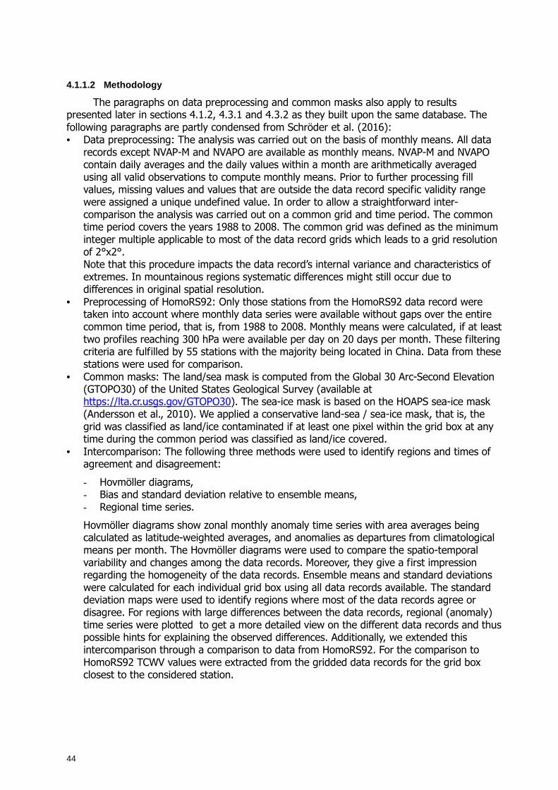
44

4.1.1.2 Methodology

The paragraphs on data preprocessing and common masks also apply to results presented later in sections 4.1.2, 4.3.1 and 4.3.2 as they built upon the same database. The following paragraphs are partly condensed from Schröder et al. (2016): • Data preprocessing: The analysis was carried out on the basis of monthly means. All data

records except NVAP-M and NVAPO are available as monthly means. NVAP-M and NVAPO contain daily averages and the daily values within a month are arithmetically averaged using all valid observations to compute monthly means. Prior to further processing fill values, missing values and values that are outside the data record specific validity range were assigned a unique undefined value. In order to allow a straightforward inter-comparison the analysis was carried out on a common grid and time period. The common time period covers the years 1988 to 2008. The common grid was defined as the minimum integer multiple applicable to most of the data record grids which leads to a grid resolution of 2°x2°. Note that this procedure impacts the data record’s internal variance and characteristics of extremes. In mountainous regions systematic differences might still occur due to differences in original spatial resolution.

• Preprocessing of HomoRS92: Only those stations from the HomoRS92 data record were taken into account where monthly data series were available without gaps over the entire common time period, that is, from 1988 to 2008. Monthly means were calculated, if at least two profiles reaching 300 hPa were available per day on 20 days per month. These filtering criteria are fulfilled by 55 stations with the majority being located in China. Data from these stations were used for comparison.

• Common masks: The land/sea mask is computed from the Global 30 Arc-Second Elevation (GTOPO30) of the United States Geological Survey (available at https://lta.cr.usgs.gov/GTOPO30). The sea-ice mask is based on the HOAPS sea-ice mask (Andersson et al., 2010). We applied a conservative land-sea / sea-ice mask, that is, the grid was classified as land/ice contaminated if at least one pixel within the grid box at any time during the common period was classified as land/ice covered.

• Intercomparison: The following three methods were used to identify regions and times of agreement and disagreement:

- Hovmöller diagrams, - Bias and standard deviation relative to ensemble means, - Regional time series.

Hovmöller diagrams show zonal monthly anomaly time series with area averages being calculated as latitude-weighted averages, and anomalies as departures from climatological means per month. The Hovmöller diagrams were used to compare the spatio-temporal variability and changes among the data records. Moreover, they give a first impression regarding the homogeneity of the data records. Ensemble means and standard deviations were calculated for each individual grid box using all data records available. The standard deviation maps were used to identify regions where most of the data records agree or disagree. For regions with large differences between the data records, regional (anomaly) time series were plotted to get a more detailed view on the different data records and thus possible hints for explaining the observed differences. Additionally, we extended this intercomparison through a comparison to data from HomoRS92. For the comparison to HomoRS92 TCWV values were extracted from the gridded data records for the grid box closest to the considered station.

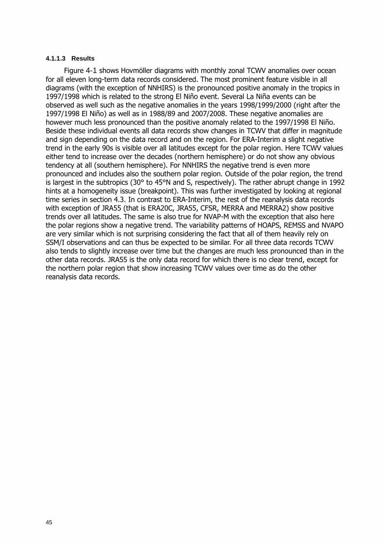
45

4.1.1.3 Results

Figure 4-1 shows Hovmöller diagrams with monthly zonal TCWV anomalies over ocean for all eleven long-term data records considered. The most prominent feature visible in all diagrams (with the exception of NNHIRS) is the pronounced positive anomaly in the tropics in 1997/1998 which is related to the strong El Niño event. Several La Niña events can be observed as well such as the negative anomalies in the years 1998/1999/2000 (right after the 1997/1998 El Niño) as well as in 1988/89 and 2007/2008. These negative anomalies are however much less pronounced than the positive anomaly related to the 1997/1998 El Niño. Beside these individual events all data records show changes in TCWV that differ in magnitude and sign depending on the data record and on the region. For ERA-Interim a slight negative trend in the early 90s is visible over all latitudes except for the polar region. Here TCWV values either tend to increase over the decades (northern hemisphere) or do not show any obvious tendency at all (southern hemisphere). For NNHIRS the negative trend is even more pronounced and includes also the southern polar region. Outside of the polar region, the trend is largest in the subtropics (30° to 45°N and S, respectively). The rather abrupt change in 1992 hints at a homogeneity issue (breakpoint). This was further investigated by looking at regional time series in section 4.3. In contrast to ERA-Interim, the rest of the reanalysis data records with exception of JRA55 (that is ERA20C, JRA55, CFSR, MERRA and MERRA2) show positive trends over all latitudes. The same is also true for NVAP-M with the exception that also here the polar regions show a negative trend. The variability patterns of HOAPS, REMSS and NVAPO are very similar which is not surprising considering the fact that all of them heavily rely on SSM/I observations and can thus be expected to be similar. For all three data records TCWV also tends to slightly increase over time but the changes are much less pronounced than in the other data records. JRA55 is the only data record for which there is no clear trend, except for the northern polar region that show increasing TCWV values over time as do the other reanalysis data records.

46

Figure 4-1: Hovmöller diagrams for 21 years of monthly zonal TCWV anomalies [%] over ocean for all

long-term data records (top to bottom): ERA-Interim, ERA20C, JRA55, CFSR (leftmost row), MERRA, MERRA2, NVAPM, NNHIRS (middle row), HOAPS, REMSS, NVAPO (rightmost row).

Over land the temporal variability is much more pronounced and the patterns of variability vary more obviously between bands of latitude compared to the ocean areas, as can be see from Figure 4-2. The latter exemplarily shows Hovmöller diagrams for three of the eight data records with valid data over land areas, namely ERA-Interim, NVAP-M and NNHIRS. The rest of the reanalysis data records show variability patterns that are very similar to ERA-Interim and are therefore not shown in Figure 4-2. The variability patterns of the reanalysis data records differ however a lot from the ones based on data of the two satellite-based data records. In case of the latter the variably patterns are not only much stronger pronounced but also differ much more between the latitude bands and show clear trends and tentative breakpoints (inhomogeneities). Such tentative breakpoints are visible for NVAPM for example in 1992 and 2002 over the northern midlatitudes (that is 30 to 45°N), in 1994 around 30°N and 30-45°S and in 1995 over the equator region. In case of NNHIRS, the dominant breakpoint feature over ocean around 1992 (see Figure 4-1) does not show up, with exception of the southern polar region. Instead NNHIRS TCWV anomalies show tentative breakpoints in 1996/1997 over the northern and southern subtropics as wells over the northern midlatitudes. In order to find out which regions exactly are affected by these rather large differences ensemble mean and standard deviations were calculated which are plotted in Figure 4-3. Regions with large standard deviations point at large differences between the data records. As expected from the Hovmöller diagrams the standard deviations are rather low over ocean with relative standard deviations generally below 15%, whereas over land regions are found reaching values larger than 25%, especially in the polar, desert and high mountain regions.

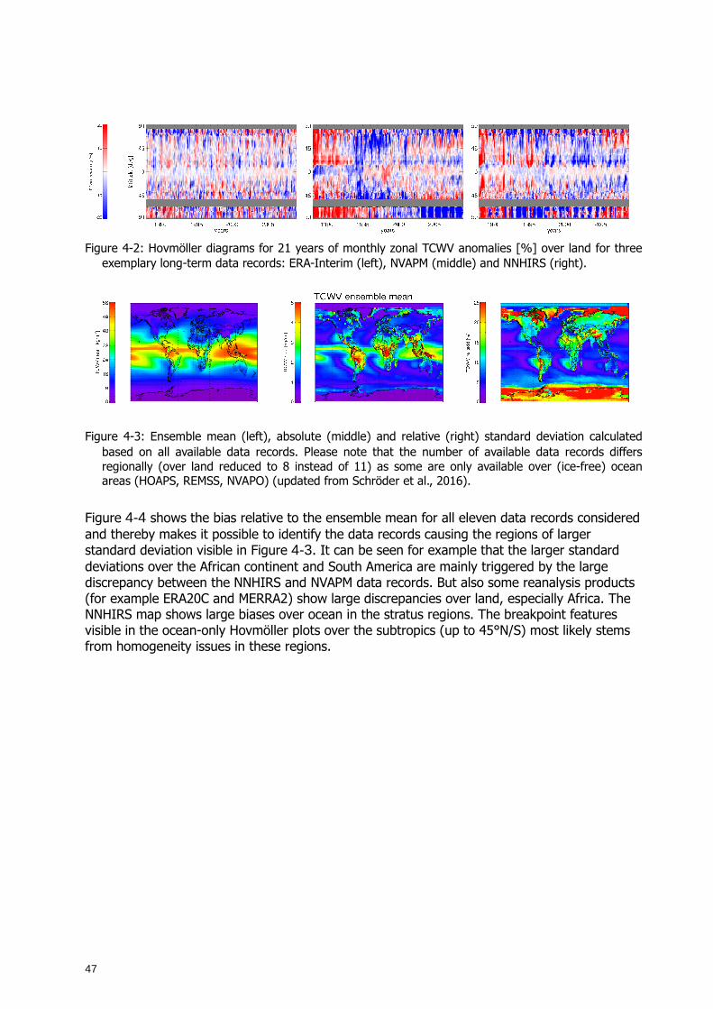
47

Figure 4-2: Hovmöller diagrams for 21 years of monthly zonal TCWV anomalies [%] over land for three

exemplary long-term data records: ERA-Interim (left), NVAPM (middle) and NNHIRS (right).

Figure 4-3: Ensemble mean (left), absolute (middle) and relative (right) standard deviation calculated based on all available data records. Please note that the number of available data records differs regionally (over land reduced to 8 instead of 11) as some are only available over (ice-free) ocean areas (HOAPS, REMSS, NVAPO) (updated from Schröder et al., 2016).

Figure 4-4 shows the bias relative to the ensemble mean for all eleven data records considered and thereby makes it possible to identify the data records causing the regions of larger standard deviation visible in Figure 4-3. It can be seen for example that the larger standard deviations over the African continent and South America are mainly triggered by the large discrepancy between the NNHIRS and NVAPM data records. But also some reanalysis products (for example ERA20C and MERRA2) show large discrepancies over land, especially Africa. The NNHIRS map shows large biases over ocean in the stratus regions. The breakpoint features visible in the ocean-only Hovmöller plots over the subtropics (up to 45°N/S) most likely stems from homogeneity issues in these regions.

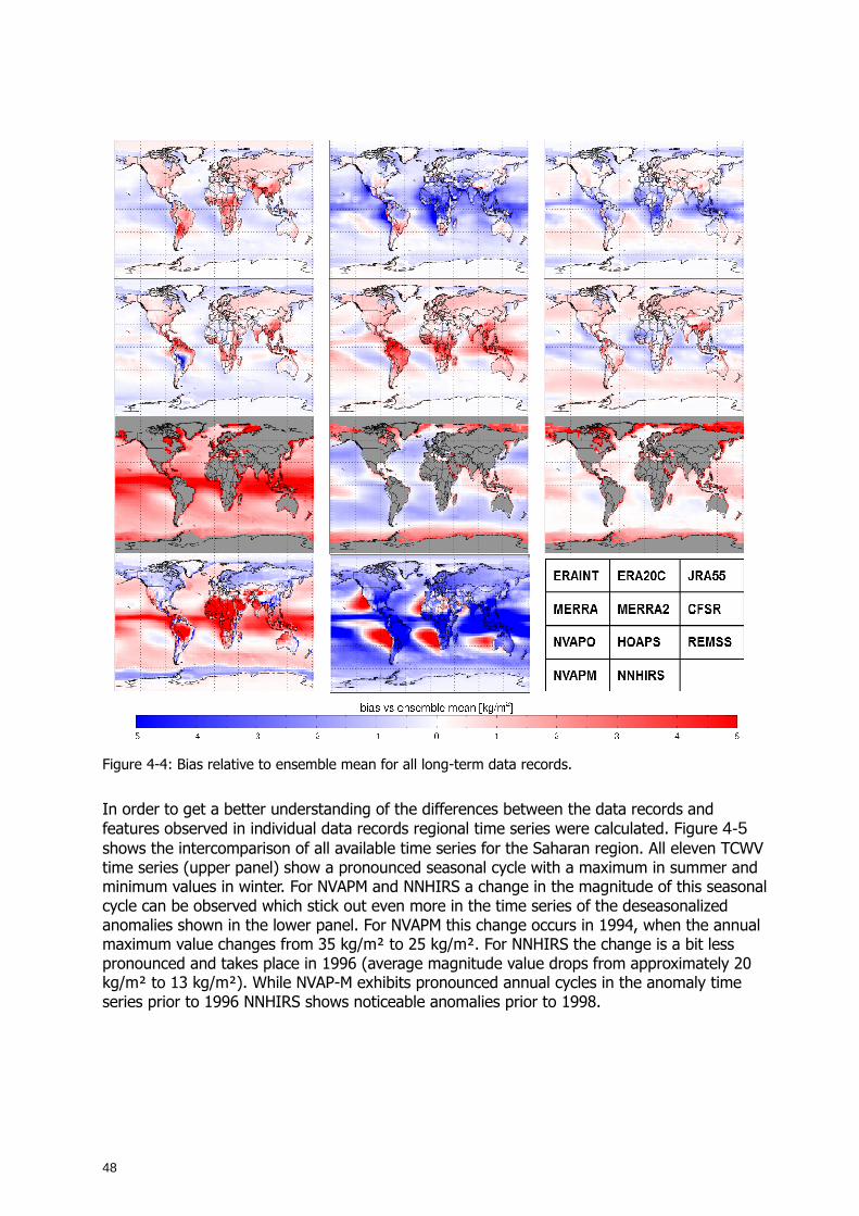
48

Figure 4-4: Bias relative to ensemble mean for all long-term data records.

In order to get a better understanding of the differences between the data records and features observed in individual data records regional time series were calculated. Figure 4-5 shows the intercomparison of all available time series for the Saharan region. All eleven TCWV time series (upper panel) show a pronounced seasonal cycle with a maximum in summer and minimum values in winter. For NVAPM and NNHIRS a change in the magnitude of this seasonal cycle can be observed which stick out even more in the time series of the deseasonalized anomalies shown in the lower panel. For NVAPM this change occurs in 1994, when the annual maximum value changes from 35 kg/m² to 25 kg/m². For NNHIRS the change is a bit less pronounced and takes place in 1996 (average magnitude value drops from approximately 20 kg/m² to 13 kg/m²). While NVAP-M exhibits pronounced annual cycles in the anomaly time series prior to 1996 NNHIRS shows noticeable anomalies prior to 1998.

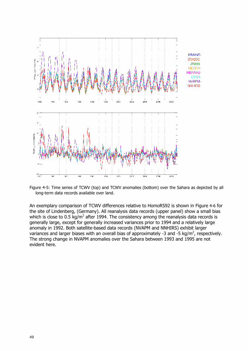
49

Figure 4-5: Time series of TCWV (top) and TCWV anomalies (bottom) over the Sahara as depicted by all long-term data records available over land.

An exemplary comparison of TCWV differences relative to HomoRS92 is shown in Figure 4-6 for the site of Lindenberg, (Germany). All reanalysis data records (upper panel) show a small bias which is close to 0.5 kg/m2 after 1994. The consistency among the reanalysis data records is generally large, except for generally increased variances prior to 1994 and a relatively large anomaly in 1992. Both satellite-based data records (NVAPM and NNHIRS) exhibit larger variances and larger biases with an overall bias of approximately -3 and -5 kg/m2, respectively. The strong change in NVAPM anomalies over the Sahara between 1993 and 1995 are not evident here.

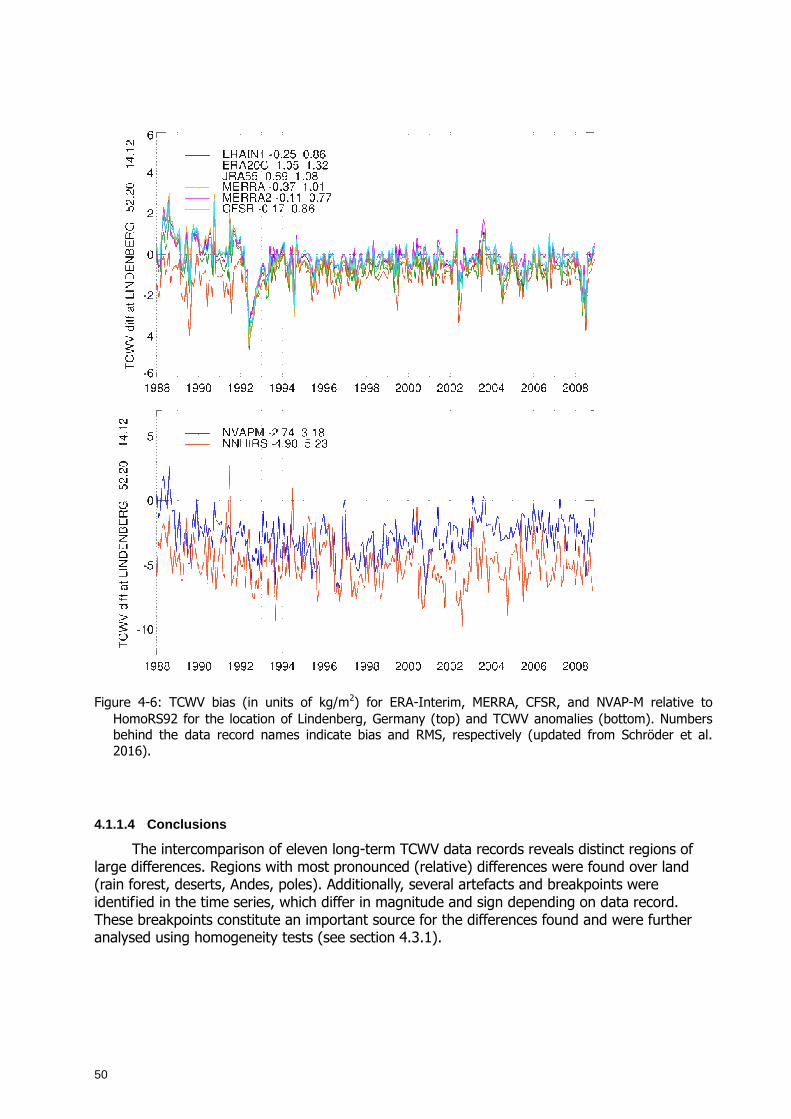
50

Figure 4-6: TCWV bias (in units of kg/m2) for ERA-Interim, MERRA, CFSR, and NVAP-M relative to

HomoRS92 for the location of Lindenberg, Germany (top) and TCWV anomalies (bottom). Numbers behind the data record names indicate bias and RMS, respectively (updated from Schröder et al. 2016).

4.1.1.4 Conclusions

The intercomparison of eleven long-term TCWV data records reveals distinct regions of large differences. Regions with most pronounced (relative) differences were found over land (rain forest, deserts, Andes, poles). Additionally, several artefacts and breakpoints were identified in the time series, which differ in magnitude and sign depending on data record. These breakpoints constitute an important source for the differences found and were further analysed using homogeneity tests (see section 4.3.1).

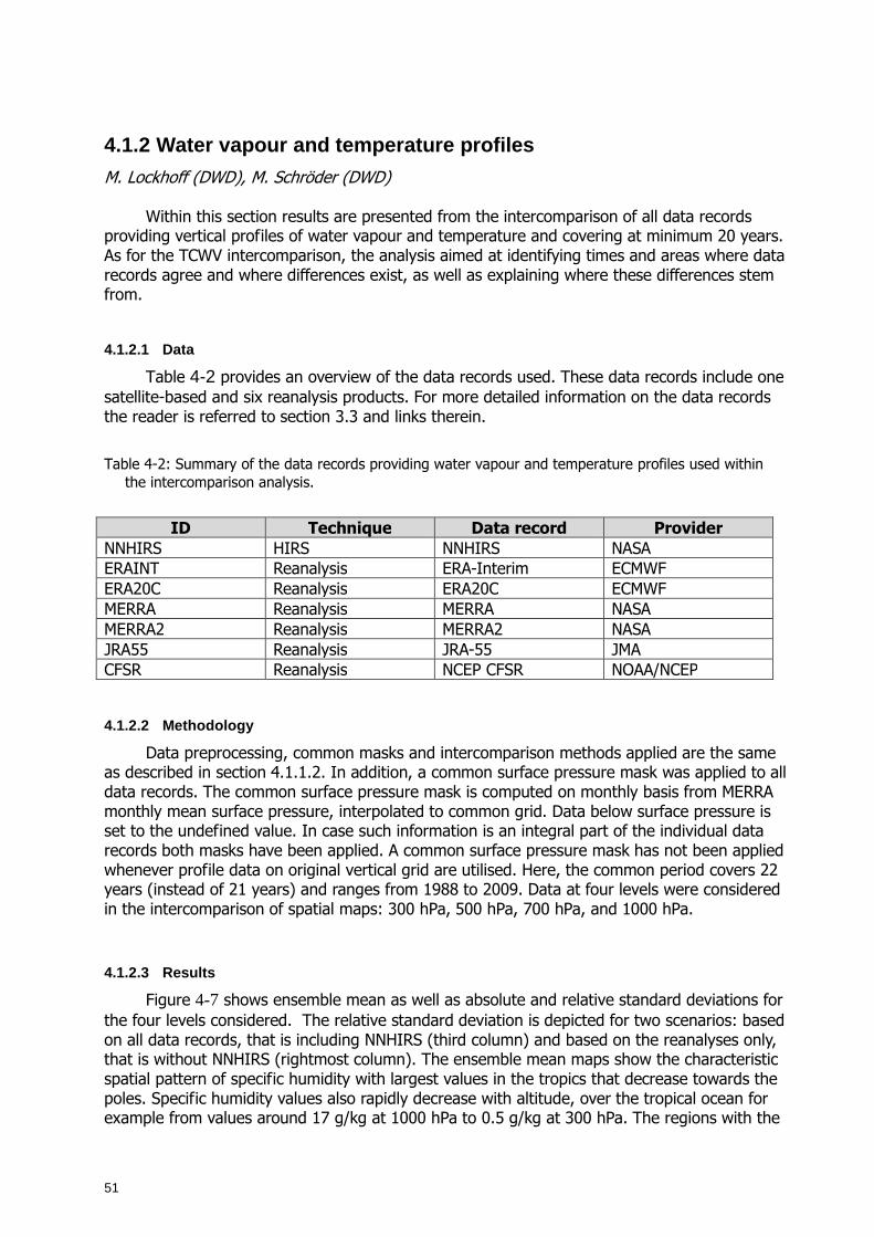
51

4.1.2 Water vapour and temperature profiles

M. Lockhoff (DWD), M. Schröder (DWD)

Within this section results are presented from the intercomparison of all data records providing vertical profiles of water vapour and temperature and covering at minimum 20 years. As for the TCWV intercomparison, the analysis aimed at identifying times and areas where data records agree and where differences exist, as well as explaining where these differences stem from.

4.1.2.1 Data

Table 4-2 provides an overview of the data records used. These data records include one satellite-based and six reanalysis products. For more detailed information on the data records the reader is referred to section 3.3 and links therein.

Table 4-2: Summary of the data records providing water vapour and temperature profiles used within the intercomparison analysis.

ID Technique Data record Provider

NNHIRS HIRS NNHIRS NASA ERAINT Reanalysis ERA-Interim ECMWF ERA20C Reanalysis ERA20C ECMWF MERRA Reanalysis MERRA NASA MERRA2 Reanalysis MERRA2 NASA JRA55 Reanalysis JRA-55 JMA CFSR Reanalysis NCEP CFSR NOAA/NCEP

4.1.2.2 Methodology

Data preprocessing, common masks and intercomparison methods applied are the same as described in section 4.1.1.2. In addition, a common surface pressure mask was applied to all data records. The common surface pressure mask is computed on monthly basis from MERRA monthly mean surface pressure, interpolated to common grid. Data below surface pressure is set to the undefined value. In case such information is an integral part of the individual data records both masks have been applied. A common surface pressure mask has not been applied whenever profile data on original vertical grid are utilised. Here, the common period covers 22 years (instead of 21 years) and ranges from 1988 to 2009. Data at four levels were considered in the intercomparison of spatial maps: 300 hPa, 500 hPa, 700 hPa, and 1000 hPa.

4.1.2.3 Results

Figure 4-7 shows ensemble mean as well as absolute and relative standard deviations for the four levels considered. The relative standard deviation is depicted for two scenarios: based on all data records, that is including NNHIRS (third column) and based on the reanalyses only, that is without NNHIRS (rightmost column). The ensemble mean maps show the characteristic spatial pattern of specific humidity with largest values in the tropics that decrease towards the poles. Specific humidity values also rapidly decrease with altitude, over the tropical ocean for example from values around 17 g/kg at 1000 hPa to 0.5 g/kg at 300 hPa. The regions with the

52

largest standard deviations differ between the four levels. Generally, the relative differences between the data records increase with increasing height. At 1000 hPa where land coverage is reduced compared to the other levels, relative standard deviations stay generally well below 15% (third column). At 700 hPa large relative differences between the data records can be found over the subtropical high pressure zones, especially over the Southern Atlantic and the Eastern Pacific. At 500 hPa, however, these same areas show lower differences compared to the surroundings. At the highest level, that is 300 hPa, differences exceeding 25% are found over large areas both over land and over ocean: for example, over Antarctica, the tropical land areas and the warm pool. When comparing the third and fourth column of Figure 4-7 it can be seen that several difference patterns outside of the tropics stem from NNHIRS. The difference among the reanalyses are most pronounced over tropical land areas with largest relative standard deviations found at 300 hPa (> 25%) as well as over Antarctica (15-20% at 300 hPa) and the tropical warm pool (15 % at 500 hPa and > 20% at 300 hPa).

The maps can in principle not be directly compared to the TCWV results (that is Figure 4-3) as the latter are based on a larger number of data records. Compared to the TCWV intercomparison there are only seven data records left and among these there is only one satellite-based data record (NNHIRS). Still, results do not change considerable when calculating ensemble mean and standard deviations for TCWV based on the reduced set of data records (not shown here). The areas of large differences stay the same with exception of reduced standard deviation values over the African continent (which were mainly triggered by NVAPM) and over the Northern polar ocean areas (which was mainly triggered by SSMI-only data records). Some of the regions with large standard deviations identified in the TCWV intercomparison also pop up in the intercomparison of the profile data records: The Arctic and Antarctic, mountainous regions such as the Andes as well as the subtropical high pressure zones. Additionally, there are new regions with high standard deviations which were not visible in the TCWV maps, such as the Western African region, the region in the Northeastern part of Southern America and the ocean areas located within the latitude band between 0 and 20°S in the Southern Pacific, Southern Atlantic and Indian Ocean (high pressure zones). However, a closer look at Figure 4-4 reveals that ERA-Interim and MERRA2 already showed larger (absolute) discrepancies from the ensemble mean in some of the regions.

Figure 4-8 shows ensemble mean and absolute standard deviations based on all temperature data records. On the ensemble mean maps one can clearly distinguish east-west temperature bands at all levels reflecting the general decrease of insolation from the equator towards the poles. Moreover, the selected levels nicely show the decrease in temperature with increasing altitude: at the 300 hPa level temperatures are around 50-60 K lower compared to 1000 hPa. When looking at the ensemble standard deviation based on all data records, it can be seen that, as for WV, largest values are generally found at the uppermost level (300 hPa), except close to surface. At 300 hPa, the differences in terms of standard deviation units between the data records regionally range from 0.6 K (over Europe, North America and parts of the subtropical land and ocean areas) to 1.5 K in the polar regions of both hemispheres. The polar regions at 1000 hPa and 700 hPa exhibit standard deviations in the same order of magnitude as for 300 hPa, especially in the southern hemisphere. Compared to WV maps the feature of large differences between the data records over the tropics is not present in the temperature maps. Thus, the observed feature in WV maps can not be attributed to discrepancies in the temperature. The same holds for other pronounced difference features in the WV maps with exception of the polar region where both WV and temperature maps exhibit larger differences between the data records considered. At 1000 hPa, the increased standard deviation values over ocean between 20° and 40° of latitude in both hemispheres in the zones of the subtropics high pressure areas can be attributed to NNHIRS as they disappear when calculating the ensemble statistics solely based on the reanaylsis data records. The same behaviour was

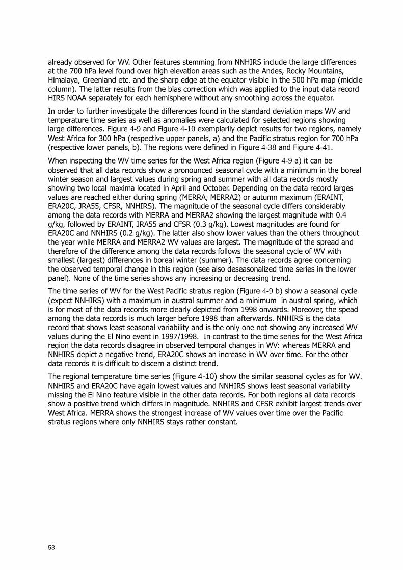
53

already observed for WV. Other features stemming from NNHIRS include the large differences at the 700 hPa level found over high elevation areas such as the Andes, Rocky Mountains, Himalaya, Greenland etc. and the sharp edge at the equator visible in the 500 hPa map (middle column). The latter results from the bias correction which was applied to the input data record HIRS NOAA separately for each hemisphere without any smoothing across the equator.

In order to further investigate the differences found in the standard deviation maps WV and temperature time series as well as anomalies were calculated for selected regions showing large differences. Figure 4-9 and Figure 4-10 exemplarily depict results for two regions, namely West Africa for 300 hPa (respective upper panels, a) and the Pacific stratus region for 700 hPa (respective lower panels, b). The regions were defined in Figure 4-38 and Figure 4-41.

When inspecting the WV time series for the West Africa region (Figure 4-9 a) it can be observed that all data records show a pronounced seasonal cycle with a minimum in the boreal winter season and largest values during spring and summer with all data records mostly showing two local maxima located in April and October. Depending on the data record larges values are reached either during spring (MERRA, MERRA2) or autumn maximum (ERAINT, ERA20C, JRA55, CFSR, NNHIRS). The magnitude of the seasonal cycle differs considerably among the data records with MERRA and MERRA2 showing the largest magnitude with 0.4 g/kg, followed by ERAINT, JRA55 and CFSR (0.3 g/kg). Lowest magnitudes are found for ERA20C and NNHIRS (0.2 g/kg). The latter also show lower values than the others throughout the year while MERRA and MERRA2 WV values are largest. The magnitude of the spread and therefore of the difference among the data records follows the seasonal cycle of WV with smallest (largest) differences in boreal winter (summer). The data records agree concerning the observed temporal change in this region (see also deseasonalized time series in the lower panel). None of the time series shows any increasing or decreasing trend.

The time series of WV for the West Pacific stratus region (Figure 4-9 b) show a seasonal cycle (expect NNHIRS) with a maximum in austral summer and a minimum in austral spring, which is for most of the data records more clearly depicted from 1998 onwards. Moreover, the spead among the data records is much larger before 1998 than afterwards. NNHIRS is the data record that shows least seasonal variability and is the only one not showing any increased WV values during the El Nino event in 1997/1998. In contrast to the time series for the West Africa region the data records disagree in observed temporal changes in WV: whereas MERRA and NNHIRS depict a negative trend, ERA20C shows an increase in WV over time. For the other data records it is difficult to discern a distinct trend.

The regional temperature time series (Figure 4-10) show the similar seasonal cycles as for WV. NNHIRS and ERA20C have again lowest values and NNHIRS shows least seasonal variability missing the El Nino feature visible in the other data records. For both regions all data records show a positive trend which differs in magnitude. NNHIRS and CFSR exhibit largest trends over West Africa. MERRA shows the strongest increase of WV values over time over the Pacific stratus regions where only NNHIRS stays rather constant.

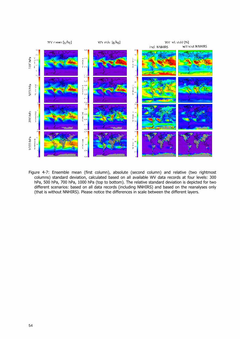
54

Figure 4-7: Ensemble mean (first column), absolute (second column) and relative (two rightmost columns) standard deviation, calculated based on all available WV data records at four levels: 300 hPa, 500 hPa, 700 hPa, 1000 hPa (top to bottom). The relative standard deviation is depicted for two different scenarios: based on all data records (including NNHIRS) and based on the reanalyses only (that is without NNHIRS). Please notice the differences in scale between the different layers.

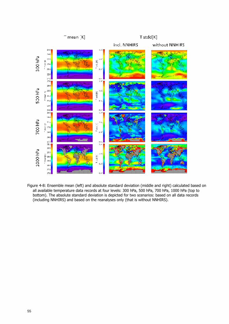
55

Figure 4-8: Ensemble mean (left) and absolute standard deviation (middle and right) calculated based on

all available temperature data records at four levels: 300 hPa, 500 hPa, 700 hPa, 1000 hPa (top to bottom). The absolute standard deviation is depicted for two scenarios: based on all data records (including NNHIRS) and based on the reanalyses only (that is without NNHIRS).

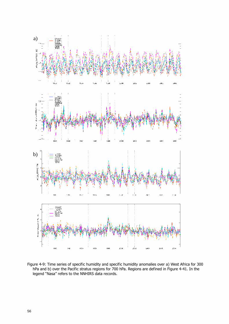
56

Figure 4-9: Time series of specific humidity and specific humidity anomalies over a) West Africa for 300 hPa and b) over the Pacific stratus regions for 700 hPa. Regions are defined in Figure 4-41. In the legend “Nasa” refers to the NNHIRS data records.

b)

a)

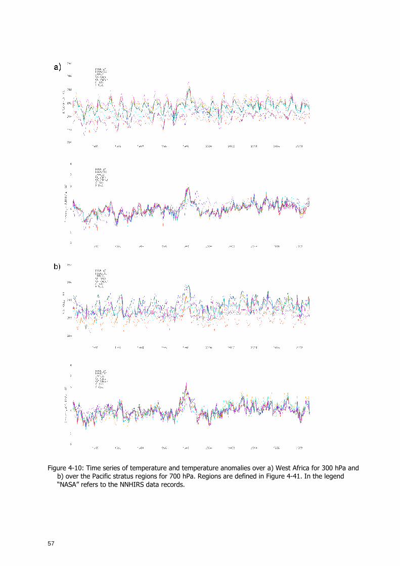
57

Figure 4-10: Time series of temperature and temperature anomalies over a) West Africa for 300 hPa and

b) over the Pacific stratus regions for 700 hPa. Regions are defined in Figure 4-41. In the legend “NASA” refers to the NNHIRS data records.

58

4.1.2.4 Conclusions

The regions of large differences identified for WV and temperature data records are generally not identical with those found for TCWV. New regions include for example Western Africa, the Northeastern part of Southern America and subtropical high pressure zones located within the latitude band between 0° and 20°S in the Southern Pacific, Southern Atlantic and Indian Ocean. The regions of largest differences vary depending on the altitude: 1000 hPa (land), 700 hPa (WV: ocean regions, temperature land and ocean), 500 hPa (tropical and substropical ocean and land areas for WV and temperature respectively), 300 hPa (land). Regional anomaly time series reveal that, depending on the region, the differences can be attributed for example to a rather constant offset between the data records (e.g. for WV over West Africa) or to differences in the respective trends of the data records (e.g. for WV over Pacific stratus region). The latter might be caused again by the presence of inhomogeneities (breakpoints) in the WV and temperature data series. The homogeneities were therefore further analysed using homogeneity tests (see section 4.3.2).

4.1.3 UTH

Q. Yang (U. Washington), L. Shi (NOAA), M. Schröder (DWD)

Water vapour is the most prominent greenhouse gas and about 60% of the natural greenhouse effect can be explained with water vapour opacity in the atmosphere (Kiehl and Trenberth, 1997). While upper tropospheric water vapour only account for a small fraction of the total water vapour mass, it accounts for a large part of the atmospheric greenhouse effect and is believed to be an important amplifier of climate change (Held and Soden, 2000). Changes in upper tropospheric water vapour in response to warming climate and its feedback on climate have been the subject of debate (IPCC, 2007). It is thus important to produce accurate, continuous observational records of upper tropospheric water vapour.

Satellite data records from microwave measurements (polar orbiting satellites) and infrared measurements (polar orbiting and geostationary) are available for monitoring the UTH. However, there are differences among these instrument observations, including differences in radiative properties of the observing channels and differences in vertical and temporal sampling. In this study, we compare three available upper tropospheric water vapour measurements and try to address and reconcile the differences.

4.1.3.1 Data and Method

HIRS We use HIRS orbital water vapour channel brightness temperatures (version v03r00, after

Shi and Bates, 2011) from 1978 to 2014 obtained from the National Center for Environmental Information (NCEI) Climate Data Record (CDR). This data record was inter-satellite calibrated to the NOAA-12 satellite and was limb-corrected.

In this study, UTH was retrieved based on HIRS water vapour channel brightness temperatures following Soden and Bretherton (1996):

Eq. 1

where Tb (K) is the instantaneous water vapour channel brightness temperature and P0 is the pressure (hPa) at the 240K-isotherm divided by 300 hPa. The parameters a = 31.5 and b =

59

0.115 K-1 are taken from Soden and Bretherton (1996). Tb with values lower than 226 K, are removed according to Gierens et al. (2004).

AMSU/MHS AMSU-B and MHS on board NOAA and Metop satellites have a 183±1 GHz channel whose

spectral characteristics are comparable to those of the 6.7 µm channel (Chung et al., 2011). Monthly mean UTH (version 2009) were obtained from Satellite Atmospheric Science Group (SASG) of Lulea University of Technology (http://www.sat.ltu.se/projects/uth-clim/). This data record was not intersatellite calibrated. Thus, we have included a new intersatellite-calibrated long-term AMSU/MHS Tb data record provided by University of Miami (Chung et al., 2013). The time series of UTH was then derived following the same retrieval method of SASG with parameters of a = 16.474 and b = 0.0702169 K-1 in Eq. 1 (Buehler and John, 2005). The SASG data is used in section 4.1 and the U. Miami data is used in section 4.2.

Chung et al. (2013) also provides regression coefficients to convert the intersatellite-calibrated AMSU/MHS Tb data record into UTH. The difference between the applications of the Chung et al. (2013) and Buehler and John (2005) coefficients to the U. Miami intersatellite-calibrated Tb data leads to an average difference of approximately 29% in UTH.

MVIRI/SEVIRI MVIRI radiances and cloud information is taken from ISCCP-DX while SEVIRI data is

extracted from DWD archive. During preprocessing for the retrieval MVIRI and SEVIRI observations are spectrally and radiometrically calibrated to Meteosat-5 (Picon et al., 2003) and HIRS onboard NOAA-12 respectively (Breon et al., 2000 and Brogniez et al., 2006). The UTH is retrieved under clear sky and low cloud conditions (similar to Eq. 1, see Schröder et al., 2014 for details). The monthly UTH was averaged from 3 hourly images within each month and version 1 product was obtained from the CM SAF (http://wui.cmsaf.eu/safira/action/viewProduktList?dId=5) with a spatial resolution of 0.625o for the period 1983 – 2009. The current data covers the region of 45°S – 45°N, 45° W – 45°E. In this study, the Meteosat UTH was re-gridded to have a spatial resolution of 2.5°x2.5°. More details can be found in Schröder et al. (2014).

4.1.3.2 Results

Geographical distributions Figure 4-11 shows the geographical distributions of mean UTH from HIRS Metop satellite,

MHS Metop satellite and Meteosat averaged over December 2007 - February 2008. The SASG product from MHS observations is used in the comparison. The spatial resolution is 2.5°x2.5°. All three data records demonstrate notable geographic variations of UTH that are consistent with regions of deep convections. In particular, the UTH displays maxima over the western Pacific warm pool and monsoonal regions of central Africa and northern Brazil. Compared with MHS, UTH from HIRS is generally drier in the tropics except for the convective cloudy regions where HIRS has significantly wetter UTH (Figure 4-11, Figure 4-12 and Figure 4-14). The high UTH from HIRS is due to low values of the water vapour channel Tb. Whether these low Tb are cloud-contaminated is subject to future studies.

We restricted the spatial coverage to 20°S – 20°N, 45° W – 45°E in the following comparisons, to fit to the Meteosat area. Averaged over the region of 20°S – 20°N, 45° W – 45°E, the UTH from MHS is about 22% and 26% higher than UTH retrieved from HIRS and Meteosat, respectively (Figure 4-14 (d and f)). UTH from HIRS is comparable to that from Meteosat

60

(Figure 4-13 and Figure 4-14(b)). Averaged over the region, HIRS UTH is about 4% higher than Meteosat (Figure 4-14 (e)). Relatively larger scatter is found in the scatterplot of HIRS-Meteosat and HIRS-MHS compared with the scatterplot of MHS-Meteosat. One possible reason for the larger scatter is that HIRS is column-clear-sky while MHS observes under almost all skies and Meteosat is clear sky and above low level clouds. Therefore, Meteosat is smoother and exhibits larger correlation with MHS. John et al. (2011) assessed the clear sky bias by subsampling the UTH product from AMSU. They observe a bias between clear-sky and almost-all-sky observations of 9 %RH for daily area weighted tropical averages which can be as large as 50% in convective regions. Also, Shi et al. (2013) analysed the difference between HIRS and AMSU-B Tb. They found a difference of about 7-10 K, depending on observed Tb. The microwave observations are warmer due to differences in emissivity and SRF, with AMSU-B peaking lower in the atmosphere. Other factors can be misclassified clouds and differences in absolute radiometric calibration.

HIRS makes two measurements per day at a given point while the Meteosat UTH product has a 3 hourly temporal resolution. We collocated HIRS Metop with Meteosat over 2007/12 -- 2008/02 to get more insights into the difference between HIRS and Meteosat UTH. We also constrain the collocation points to locate within 20°S-20°N. In total, there are 17433 collocated points. The collocated tracks are shown in Figure 4-15. On average, HIRS UTH is about 21% wetter than Meteosat at the collocated points (Figure 4-16). As in Figure 4-14, a large scatter of the HIRS and Meteosat UTH is seen (Figure 4-16 (c)) which can be explained with differences in cloud sampling.

Besides differences in SRF and absolute calibration different weighting functions were utilised during retrieval design. Thus, we used the RTTOV9.3 model (Matricardi et al., 2004) and the training profile data base described in Schröder et al. (2014) to compute the relative humidity Jacobians JRH for Meteosat5 and HIRS on NOAA-12. Using these JRH and the weighting function defined in Soden and Bretherton (1996) as averaging kernels for the profile data base differences in UTH and in the peak height of the averaging kernel as a function of spectral response function (HIRS on NOAA-12, Meteosat5) and weighting function (JRH and after Soden and Bretherton, 1996, SB96) were assessed. JRH was used during the Meteosat retrieval development (Brogniez et al., 2009; Schröder et al., 2014) while the HIRS retrieval relies on the work of Soden and Bretherton (1996). Figure 4-17 shows the PDF of the peak height of the weighting functions used during HIRS and Meteosat retrieval. The maxima of the PDFs are at the same bin. However, Meteosat PDF exhibits a more realistic wider spread. Figure 4-17 shows a scatter plot of UTH using the JRH, SB96 and the Meteosat5 SRF. The UTH computed using the SB96 weighting function introduces a 23.3% relative bias. We also computed this difference using the HIRS spectral response function as basis and found a statistically insignificant difference to the Meteosat case. Also, the difference between UTH as function of JRH and HIRS SRF and as function of JRH and Meteosat SRF is negligible (0.0% relative). The above difference of ~23% is consistent with the 21% relative difference at collocation points between HIRS and Meteosat. Therefore, the observed difference between HIRS and Meteosat can be largely explained by the different weighting functions used during retrieval design. Also, the uncertainty of a SB96 based retrieval exhibits a larger uncertainty relative to a JRH based retrieval scheme (Brogniez et al., 2009; Schröder et al., 2014).

Note that the climatological difference between HIRS and Meteosat is 4%. Thus, sampling differences lead to a relative difference of about 19%. It seems that differences in temporal sampling and in particular in clear sky versus clear sky and low level cloud cases explain this difference (see also discussion in Brogniez et al., 2006). Differences in spatial sampling also contribute to the sampling bias (not shown).

61

Figure 4-11: Geographical distributions of mean UTH (%) from HIRS Metop, MHS Metop and Meteosat averaged over 2007/12 - 2008/02. The spatial resolution is 2.5° by 2.5°.

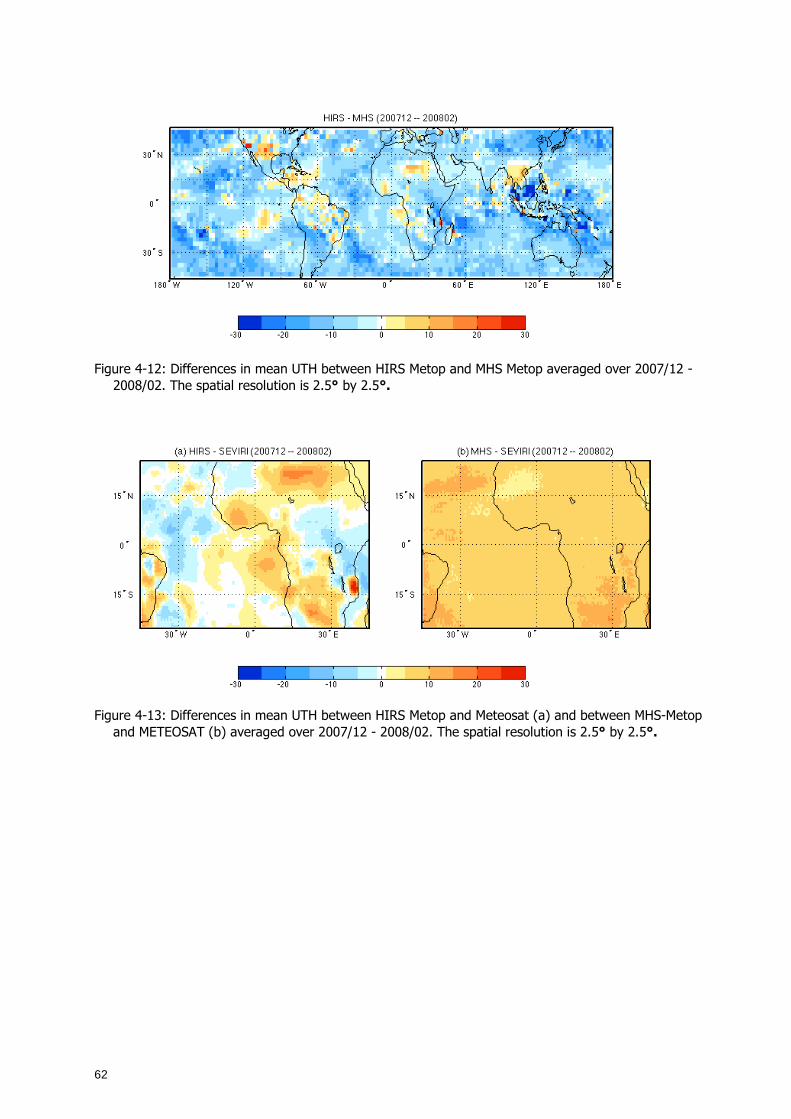
62

Figure 4-12: Differences in mean UTH between HIRS Metop and MHS Metop averaged over 2007/12 - 2008/02. The spatial resolution is 2.5° by 2.5°.

Figure 4-13: Differences in mean UTH between HIRS Metop and Meteosat (a) and between MHS-Metop and METEOSAT (b) averaged over 2007/12 - 2008/02. The spatial resolution is 2.5° by 2.5°.

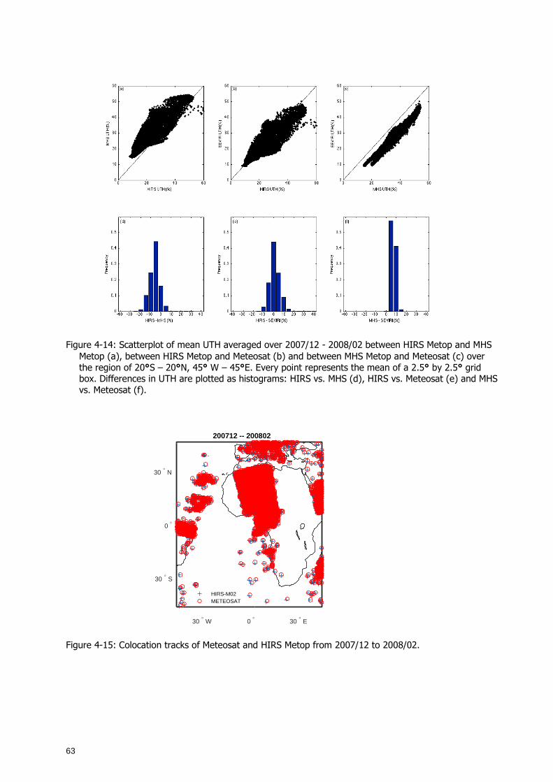
63

Figure 4-14: Scatterplot of mean UTH averaged over 2007/12 - 2008/02 between HIRS Metop and MHS Metop (a), between HIRS Metop and Meteosat (b) and between MHS Metop and Meteosat (c) over the region of 20°S – 20°N, 45° W – 45°E. Every point represents the mean of a 2.5° by 2.5° grid box. Differences in UTH are plotted as histograms: HIRS vs. MHS (d), HIRS vs. Meteosat (e) and MHS vs. Meteosat (f).

30 ° W 0 ° 30 ° E

30 ° S

0 °

30 ° N

200712 -- 200802

HIRS-M02METEOSAT

Figure 4-15: Colocation tracks of Meteosat and HIRS Metop from 2007/12 to 2008/02.

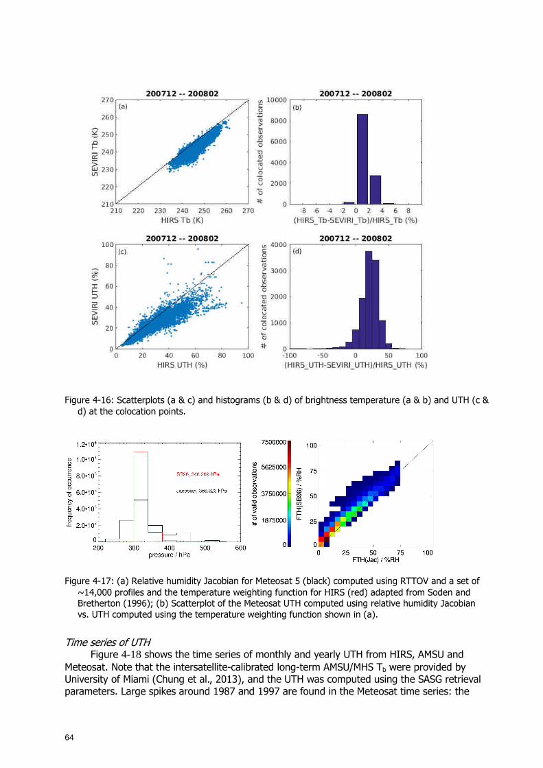
64

Figure 4-16: Scatterplots (a & c) and histograms (b & d) of brightness temperature (a & b) and UTH (c & d) at the colocation points.

Figure 4-17: (a) Relative humidity Jacobian for Meteosat 5 (black) computed using RTTOV and a set of ~14,000 profiles and the temperature weighting function for HIRS (red) adapted from Soden and Bretherton (1996); (b) Scatterplot of the Meteosat UTH computed using relative humidity Jacobian vs. UTH computed using the temperature weighting function shown in (a).

Time series of UTH Figure 4-18 shows the time series of monthly and yearly UTH from HIRS, AMSU and

Meteosat. Note that the intersatellite-calibrated long-term AMSU/MHS Tb were provided by University of Miami (Chung et al., 2013), and the UTH was computed using the SASG retrieval parameters. Large spikes around 1987 and 1997 are found in the Meteosat time series: the

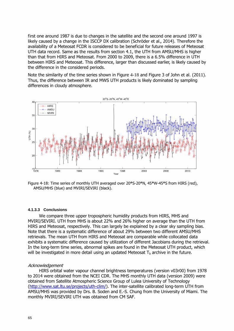
65

first one around 1987 is due to changes in the satellite and the second one around 1997 is likely caused by a change in the ISCCP DX calibration (Schröder et al., 2014). Therefore the availability of a Meteosat FCDR is considered to be beneficial for future releases of Meteosat UTH data record. Same as the results from section 4.1, the UTH from AMSU/MHS is higher than that from HIRS and Meteosat. From 2000 to 2009, there is a 6.5% difference in UTH between HIRS and Meteosat. This difference, larger than discussed earlier, is likely caused by the difference in the considered periods.

Note the similarity of the time series shown in Figure 4-18 and Figure 3 of John et al. (2011). Thus, the difference between IR and MWS UTH products is likely dominated by sampling differences in cloudy atmosphere.

Figure 4-18: Time series of monthly UTH averaged over 20°S-20°N, 45°W-45°S from HIRS (red), AMSU/MHS (blue) and MVIRI/SEVIRI (black).

4.1.3.3 Conclusions

We compare three upper tropospheric humidity products from HIRS, MHS and MVIRI/SEVIRI. UTH from MHS is about 22% and 26% higher on average than the UTH from HIRS and Meteosat, respectively. This can largely be explained by a clear sky sampling bias. Note that there is a systematic difference of about 29% between two different AMSU/MHS retrievals. The mean UTH from HIRS and Meteosat are comparable while collocated data exhibits a systematic difference caused by utilization of different Jacobians during the retrieval. In the long-term time series, abnormal spikes are found in the Meteosat UTH product, which will be investigated in more detail using an updated Meteosat Tb archive in the future.

Acknowledgement HIRS orbital water vapour channel brightness temperatures (version v03r00) from 1978

to 2014 were obtained from the NCEI CDR. The MHS monthly UTH data (version 2009) were obtained from Satellite Atmospheric Science Group of Lulea University of Technology (http://www.sat.ltu.se/projects/uth-clim/). The inter-satellite calibrated long-term UTH from AMSU/MHS was provided by Drs. B. Soden and E.-S. Chung from the University of Miami. The monthly MVIRI/SEVIRI UTH was obtained from CM SAF.

66

4.2 Variability analysis

4.2.1 TCWV

R. Bennartz (Vanderbilt U.), F. Fell (Informus GmbH), M. Schröder (DWD), A. Walther (U. Wisconsin), U. Willen (SMHI)

In total, eight TCWV climate time series comprising observational data, re-analyses as well as climate model results were analysed against a set of nine climate indices. The aims were to evaluate the different TCWV products against the climate indices and to provide information about commonalities and differences between the different data records.

The following results are a shortened version of Bennartz et al. (2014), available at http://gewex-vap.org/wp-content/uploads/2016/11/20141113_VAKAS_FinalReport.pdf.

4.2.1.1 Data

Eight different data records have been used: CFSR, EC Earth, ERA-Interim, HOAPS, MERRA, MPI-ESM, NVAP-M, and RSS. These data records can be subdivided into satellite observation based data records (HOAPS, NVAP-M, RSS), reanalyses using data assimilation techniques (CFSR, ERA-Interim, MERRA), as well as climate model derived data records that have been obtained without data assimilation but with prescribed sea surface temperature fields (EC Earth, MPI-ESM). The satellite and reanalyses products have been described in section 3.3. A brief description of the climate models follows.

EC Earth (ECE)

The EC Earth (ECE) 1-degree TCWV data record has been obtained from atmosphere only global climate model simulations, using prescribed observed sea-surface temperatures and prescribed sea ice for the period 1979-2008. The ECE global climate model (Hazeleger et al 2010) has been developed from the ECWMF model (http://ecearth.knmi.nl/). The atmospheric component is based on ECMWF's Integrated Forecasting System (IFS), cycle 31r1 with some additional implementation, including a new convection scheme and the new land surface scheme H-TESSEL. Small changes in the gravity wave drag and shortwave radiation parameterisations have also been applied to reproduce the observed climatology of the past 40 years as closely as possible and to achieve a balanced radiation budget.

For this study the model was run at T159 (125km) horizontal spectral resolution with 62 vertical levels.

MPI-ESM (ESM)

The Earth System Model of the Max Planck Institute for Meteorology (MPI-ESM) couples atmosphere, ocean and land surface through the exchange of energy, momentum, water, and important trace gases such as carbon dioxide. It has been used for comparative model calculations in the context of CMIP5, which constitute the German contribution to the Fifth Assessment Report of the IPCC (Intergovernmental Panel on Climate Change). It is based on the components of ECHAM6 for the atmosphere and MPIOM for the ocean as well as JSBACH for the terrestrial biosphere and HAMOCC for the ocean´s biogeochemistry. The coupling of atmosphere and land on the one hand and ocean and biogeochemistry on the other hand is made possible by the separate coupling program OASIS3. Energy, momentum, water and CO2 are exchanged with the help of this coupling. Further details and evaluation results can be found in Müller et al. (2012) and Pohlmann et al. (2013).

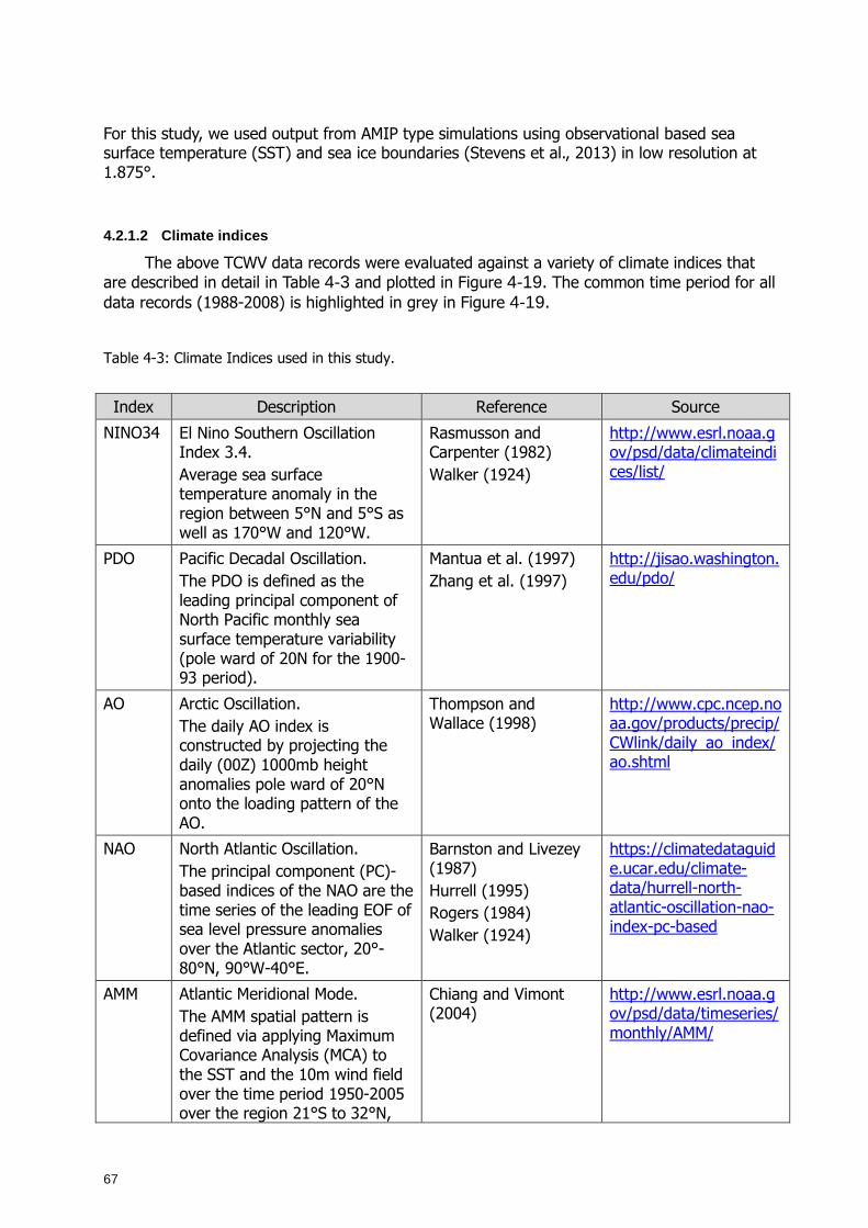
67

For this study, we used output from AMIP type simulations using observational based sea surface temperature (SST) and sea ice boundaries (Stevens et al., 2013) in low resolution at 1.875°.

4.2.1.2 Climate indices

The above TCWV data records were evaluated against a variety of climate indices that are described in detail in Table 4-3 and plotted in Figure 4-19. The common time period for all data records (1988-2008) is highlighted in grey in Figure 4-19.

Table 4-3: Climate Indices used in this study.

Index Description Reference Source

NINO34 El Nino Southern Oscillation Index 3.4. Average sea surface temperature anomaly in the region between 5°N and 5°S as well as 170°W and 120°W.

Rasmusson and Carpenter (1982) Walker (1924)

http://www.esrl.noaa.gov/psd/data/climateindices/list/

PDO Pacific Decadal Oscillation. The PDO is defined as the leading principal component of North Pacific monthly sea surface temperature variability (pole ward of 20N for the 1900-93 period).

Mantua et al. (1997) Zhang et al. (1997)

http://jisao.washington.edu/pdo/

AO Arctic Oscillation. The daily AO index is constructed by projecting the daily (00Z) 1000mb height anomalies pole ward of 20°N onto the loading pattern of the AO.

Thompson and Wallace (1998)

http://www.cpc.ncep.noaa.gov/products/precip/CWlink/daily_ao_index/ao.shtml

NAO North Atlantic Oscillation. The principal component (PC)-based indices of the NAO are the time series of the leading EOF of sea level pressure anomalies over the Atlantic sector, 20°-80°N, 90°W-40°E.

Barnston and Livezey (1987) Hurrell (1995) Rogers (1984) Walker (1924)

https://climatedataguide.ucar.edu/climate-data/hurrell-north-atlantic-oscillation-nao-index-pc-based

AMM Atlantic Meridional Mode. The AMM spatial pattern is defined via applying Maximum Covariance Analysis (MCA) to the SST and the 10m wind field over the time period 1950-2005 over the region 21°S to 32°N,

Chiang and Vimont (2004)

http://www.esrl.noaa.gov/psd/data/timeseries/monthly/AMM/

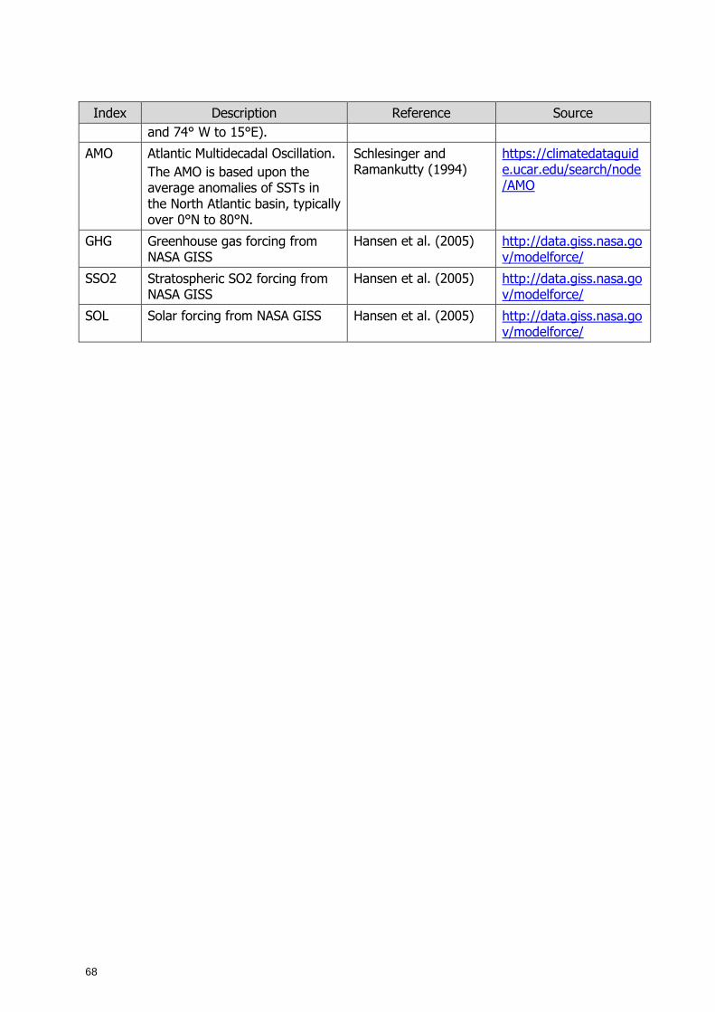
68

Index Description Reference Source

and 74° W to 15°E).

AMO Atlantic Multidecadal Oscillation. The AMO is based upon the average anomalies of SSTs in the North Atlantic basin, typically over 0°N to 80°N.

Schlesinger and Ramankutty (1994)

https://climatedataguide.ucar.edu/search/node/AMO

GHG Greenhouse gas forcing from NASA GISS

Hansen et al. (2005) http://data.giss.nasa.gov/modelforce/

SSO2 Stratospheric SO2 forcing from NASA GISS

Hansen et al. (2005) http://data.giss.nasa.gov/modelforce/

SOL Solar forcing from NASA GISS Hansen et al. (2005) http://data.giss.nasa.gov/modelforce/

69

Figure 4-19: The panels on the left show time series of the different climate indices listed in Table 4-3.

The grey-shaded area in the left panels indicates the 1988-2008 period for which satellite and other water vapour data are evaluated. The right panels show corresponding autocorrelation coefficients for lag times between zero and 12 months.

4.2.1.3 Methods

Data processing The analysis is carried out on a common grid and time period. The common grid is a

regular longitude/latitude grid with a resolution of 1°×1° and centre location of the grid boxes between the full degree values, which leads to an array size of 360×180 pixels.

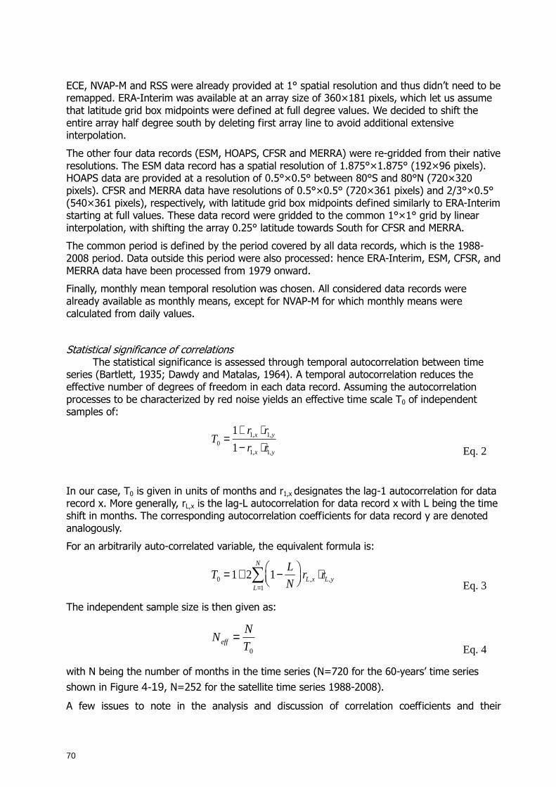
70

ECE, NVAP-M and RSS were already provided at 1° spatial resolution and thus didn’t need to be remapped. ERA-Interim was available at an array size of 360×181 pixels, which let us assume that latitude grid box midpoints were defined at full degree values. We decided to shift the entire array half degree south by deleting first array line to avoid additional extensive interpolation.

The other four data records (ESM, HOAPS, CFSR and MERRA) were re-gridded from their native resolutions. The ESM data record has a spatial resolution of 1.875°×1.875° (192×96 pixels). HOAPS data are provided at a resolution of 0.5°×0.5° between 80°S and 80°N (720×320 pixels). CFSR and MERRA data have resolutions of 0.5°×0.5° (720×361 pixels) and 2/3°×0.5° (540×361 pixels), respectively, with latitude grid box midpoints defined similarly to ERA-Interim starting at full values. These data record were gridded to the common 1°×1° grid by linear interpolation, with shifting the array 0.25° latitude towards South for CFSR and MERRA.

The common period is defined by the period covered by all data records, which is the 1988-2008 period. Data outside this period were also processed: hence ERA-Interim, ESM, CFSR, and MERRA data have been processed from 1979 onward.

Finally, monthly mean temporal resolution was chosen. All considered data records were already available as monthly means, except for NVAP-M for which monthly means were calculated from daily values.

Statistical significance of correlations The statistical significance is assessed through temporal autocorrelation between time

series (Bartlett, 1935; Dawdy and Matalas, 1964). A temporal autocorrelation reduces the effective number of degrees of freedom in each data record. Assuming the autocorrelation processes to be characterized by red noise yields an effective time scale T0 of independent samples of:

T0 =

1+ r1,x ⋅ r1,y

1− r1,x ⋅ r1,y

Eq. 2

In our case, T0 is given in units of months and r1,x designates the lag-1 autocorrelation for data record x. More generally, rL,x is the lag-L autocorrelation for data record x with L being the time shift in months. The corresponding autocorrelation coefficients for data record y are denoted analogously.

For an arbitrarily auto-correlated variable, the equivalent formula is:

T0 = 1+ 2 1− L

N

rL ,x ⋅ rL,yL=1

N

∑ Eq. 3

The independent sample size is then given as:

Neff = N

T0

Eq. 4

with N being the number of months in the time series (N=720 for the 60-years’ time series

shown in Figure 4-19, N=252 for the satellite time series 1988-2008).

A few issues to note in the analysis and discussion of correlation coefficients and their

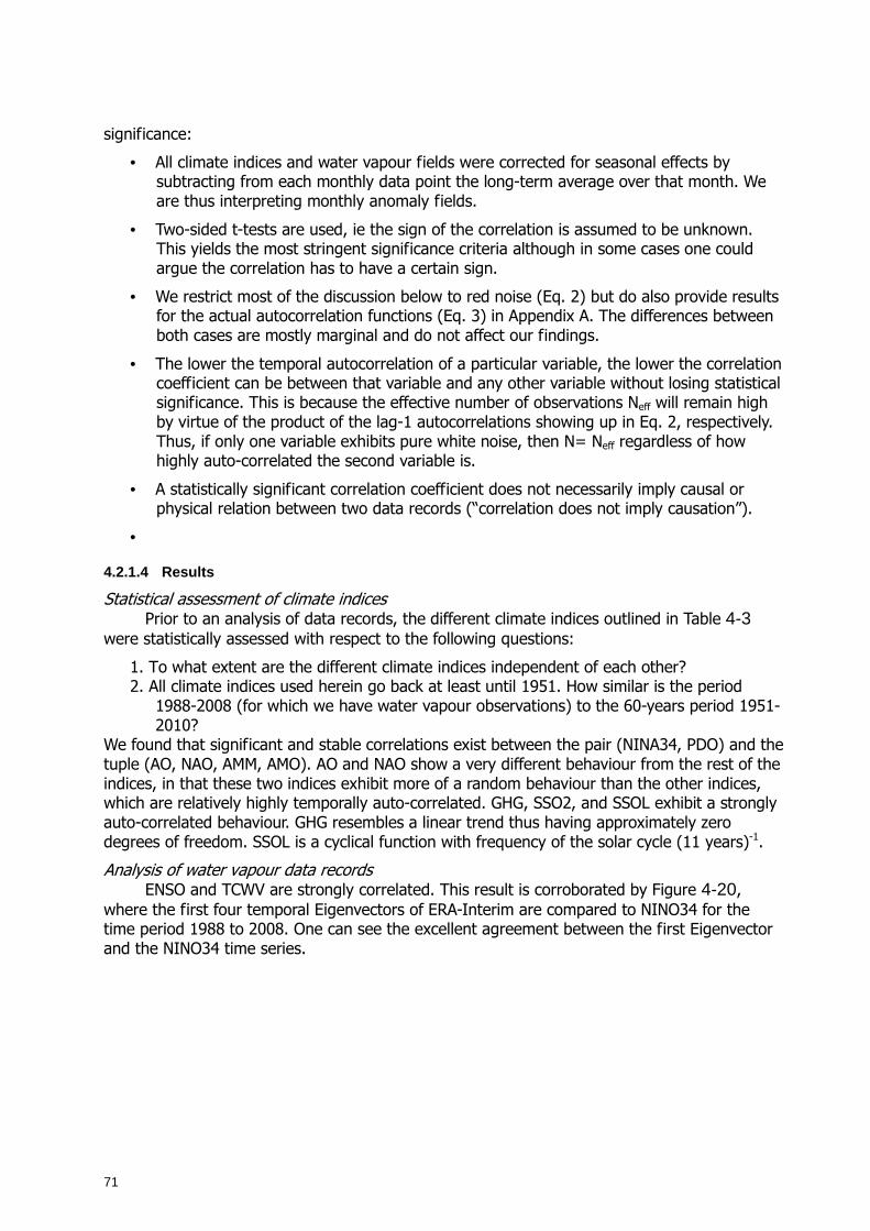
71

significance:

• All climate indices and water vapour fields were corrected for seasonal effects by subtracting from each monthly data point the long-term average over that month. We are thus interpreting monthly anomaly fields.

• Two-sided t-tests are used, ie the sign of the correlation is assumed to be unknown. This yields the most stringent significance criteria although in some cases one could argue the correlation has to have a certain sign.

• We restrict most of the discussion below to red noise (Eq. 2) but do also provide results for the actual autocorrelation functions (Eq. 3) in Appendix A. The differences between both cases are mostly marginal and do not affect our findings.

• The lower the temporal autocorrelation of a particular variable, the lower the correlation coefficient can be between that variable and any other variable without losing statistical significance. This is because the effective number of observations Neff will remain high by virtue of the product of the lag-1 autocorrelations showing up in Eq. 2, respectively. Thus, if only one variable exhibits pure white noise, then N= Neff regardless of how highly auto-correlated the second variable is.

• A statistically significant correlation coefficient does not necessarily imply causal or physical relation between two data records (“correlation does not imply causation”).

•

4.2.1.4 Results

Statistical assessment of climate indices Prior to an analysis of data records, the different climate indices outlined in Table 4-3

were statistically assessed with respect to the following questions:

1. To what extent are the different climate indices independent of each other? 2. All climate indices used herein go back at least until 1951. How similar is the period

1988-2008 (for which we have water vapour observations) to the 60-years period 1951-2010?

We found that significant and stable correlations exist between the pair (NINA34, PDO) and the tuple (AO, NAO, AMM, AMO). AO and NAO show a very different behaviour from the rest of the indices, in that these two indices exhibit more of a random behaviour than the other indices, which are relatively highly temporally auto-correlated. GHG, SSO2, and SSOL exhibit a strongly auto-correlated behaviour. GHG resembles a linear trend thus having approximately zero degrees of freedom. SSOL is a cyclical function with frequency of the solar cycle (11 years)-1.

Analysis of water vapour data records ENSO and TCWV are strongly correlated. This result is corroborated by Figure 4-20,

where the first four temporal Eigenvectors of ERA-Interim are compared to NINO34 for the time period 1988 to 2008. One can see the excellent agreement between the first Eigenvector and the NINO34 time series.

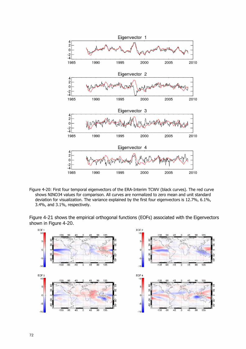
72

Figure 4-20: First four temporal eigenvectors of the ERA-Interim TCWV (black curves). The red curve shows NINO34 values for comparison. All curves are normalized to zero mean and unit standard deviation for visualization. The variance explained by the first four eigenvectors is 12.7%, 6.1%, 3.4%, and 3.1%, respectively.

Figure 4-21 shows the empirical orthogonal functions (EOFs) associated with the Eigenvectors shown in Figure 4-20.

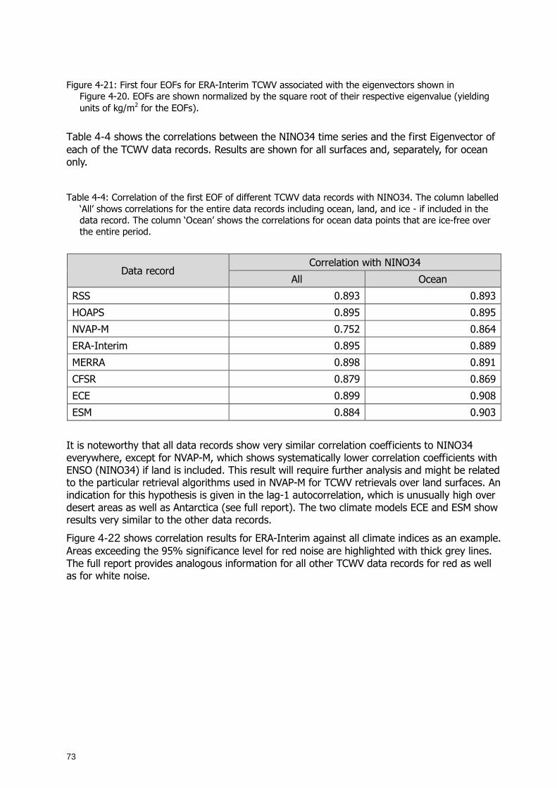
73

Figure 4-21: First four EOFs for ERA-Interim TCWV associated with the eigenvectors shown in Figure 4-20. EOFs are shown normalized by the square root of their respective eigenvalue (yielding units of kg/m2 for the EOFs).

Table 4-4 shows the correlations between the NINO34 time series and the first Eigenvector of each of the TCWV data records. Results are shown for all surfaces and, separately, for ocean only.

Table 4-4: Correlation of the first EOF of different TCWV data records with NINO34. The column labelled ‘All’ shows correlations for the entire data records including ocean, land, and ice - if included in the data record. The column ‘Ocean’ shows the correlations for ocean data points that are ice-free over the entire period.

Data record Correlation with NINO34

All Ocean

RSS 0.893 0.893

HOAPS 0.895 0.895

NVAP-M 0.752 0.864

ERA-Interim 0.895 0.889

MERRA 0.898 0.891

CFSR 0.879 0.869

ECE 0.899 0.908

ESM 0.884 0.903

It is noteworthy that all data records show very similar correlation coefficients to NINO34 everywhere, except for NVAP-M, which shows systematically lower correlation coefficients with ENSO (NINO34) if land is included. This result will require further analysis and might be related to the particular retrieval algorithms used in NVAP-M for TCWV retrievals over land surfaces. An indication for this hypothesis is given in the lag-1 autocorrelation, which is unusually high over desert areas as well as Antarctica (see full report). The two climate models ECE and ESM show results very similar to the other data records.

Figure 4-22 shows correlation results for ERA-Interim against all climate indices as an example. Areas exceeding the 95% significance level for red noise are highlighted with thick grey lines. The full report provides analogous information for all other TCWV data records for red as well as for white noise.

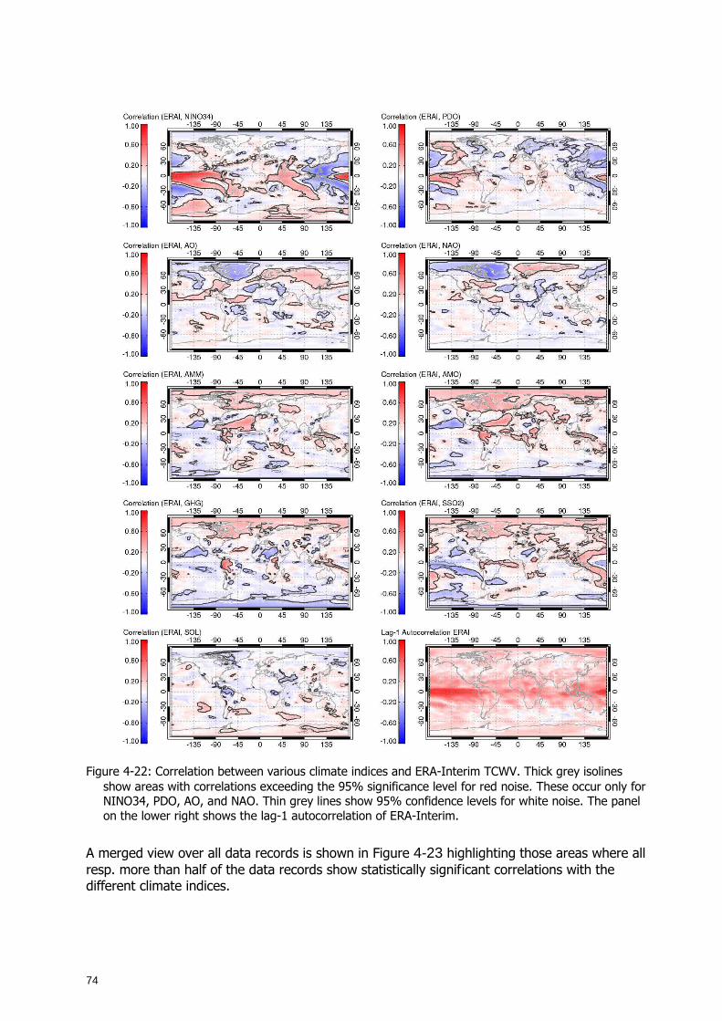
74

Figure 4-22: Correlation between various climate indices and ERA-Interim TCWV. Thick grey isolines

show areas with correlations exceeding the 95% significance level for red noise. These occur only for NINO34, PDO, AO, and NAO. Thin grey lines show 95% confidence levels for white noise. The panel on the lower right shows the lag-1 autocorrelation of ERA-Interim.

A merged view over all data records is shown in Figure 4-23 highlighting those areas where all resp. more than half of the data records show statistically significant correlations with the different climate indices.

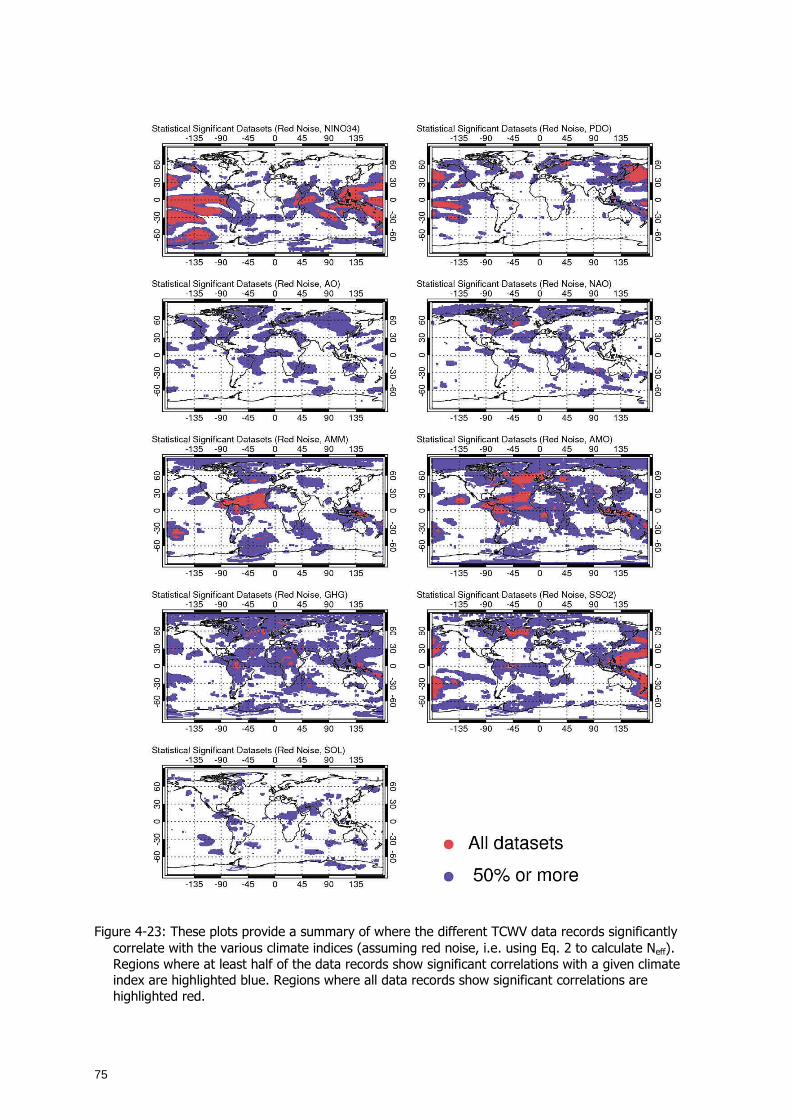
75

Figure 4-23: These plots provide a summary of where the different TCWV data records significantly correlate with the various climate indices (assuming red noise, i.e. using Eq. 2 to calculate Neff). Regions where at least half of the data records show significant correlations with a given climate index are highlighted blue. Regions where all data records show significant correlations are highlighted red.

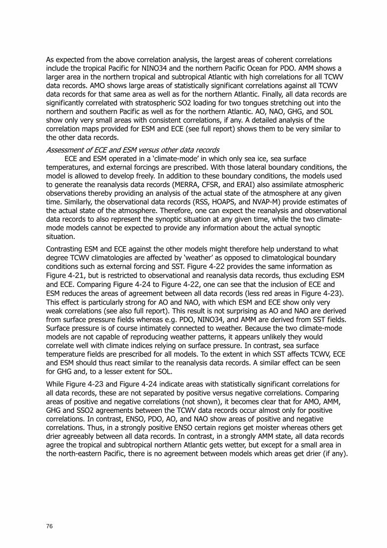
76

As expected from the above correlation analysis, the largest areas of coherent correlations include the tropical Pacific for NINO34 and the northern Pacific Ocean for PDO. AMM shows a larger area in the northern tropical and subtropical Atlantic with high correlations for all TCWV data records. AMO shows large areas of statistically significant correlations against all TCWV data records for that same area as well as for the northern Atlantic. Finally, all data records are significantly correlated with stratospheric SO2 loading for two tongues stretching out into the northern and southern Pacific as well as for the northern Atlantic. AO, NAO, GHG, and SOL show only very small areas with consistent correlations, if any. A detailed analysis of the correlation maps provided for ESM and ECE (see full report) shows them to be very similar to the other data records.

Assessment of ECE and ESM versus other data records ECE and ESM operated in a ‘climate-mode’ in which only sea ice, sea surface

temperatures, and external forcings are prescribed. With those lateral boundary conditions, the model is allowed to develop freely. In addition to these boundary conditions, the models used to generate the reanalysis data records (MERRA, CFSR, and ERAI) also assimilate atmospheric observations thereby providing an analysis of the actual state of the atmosphere at any given time. Similarly, the observational data records (RSS, HOAPS, and NVAP-M) provide estimates of the actual state of the atmosphere. Therefore, one can expect the reanalysis and observational data records to also represent the synoptic situation at any given time, while the two climate-mode models cannot be expected to provide any information about the actual synoptic situation.

Contrasting ESM and ECE against the other models might therefore help understand to what degree TCWV climatologies are affected by ‘weather’ as opposed to climatological boundary conditions such as external forcing and SST. Figure 4-22 provides the same information as Figure 4-21, but is restricted to observational and reanalysis data records, thus excluding ESM and ECE. Comparing Figure 4-24 to Figure 4-22, one can see that the inclusion of ECE and ESM reduces the areas of agreement between all data records (less red areas in Figure 4-23). This effect is particularly strong for AO and NAO, with which ESM and ECE show only very weak correlations (see also full report). This result is not surprising as AO and NAO are derived from surface pressure fields whereas e.g. PDO, NINO34, and AMM are derived from SST fields. Surface pressure is of course intimately connected to weather. Because the two climate-mode models are not capable of reproducing weather patterns, it appears unlikely they would correlate well with climate indices relying on surface pressure. In contrast, sea surface temperature fields are prescribed for all models. To the extent in which SST affects TCWV, ECE and ESM should thus react similar to the reanalysis data records. A similar effect can be seen for GHG and, to a lesser extent for SOL.

While Figure 4-23 and Figure 4-24 indicate areas with statistically significant correlations for all data records, these are not separated by positive versus negative correlations. Comparing areas of positive and negative correlations (not shown), it becomes clear that for AMO, AMM, GHG and SSO2 agreements between the TCWV data records occur almost only for positive correlations. In contrast, ENSO, PDO, AO, and NAO show areas of positive and negative correlations. Thus, in a strongly positive ENSO certain regions get moister whereas others get drier agreeably between all data records. In contrast, in a strongly AMM state, all data records agree the tropical and subtropical northern Atlantic gets wetter, but except for a small area in the north-eastern Pacific, there is no agreement between models which areas get drier (if any).

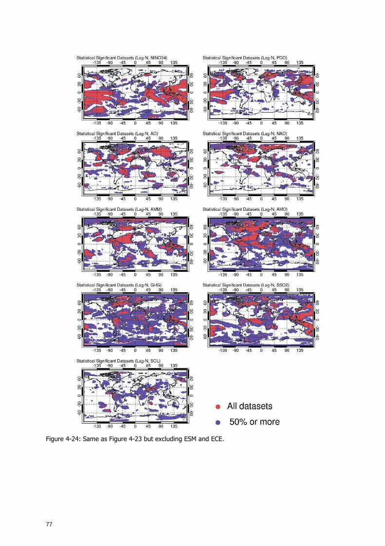
77

Figure 4-24: Same as Figure 4-23 but excluding ESM and ECE.

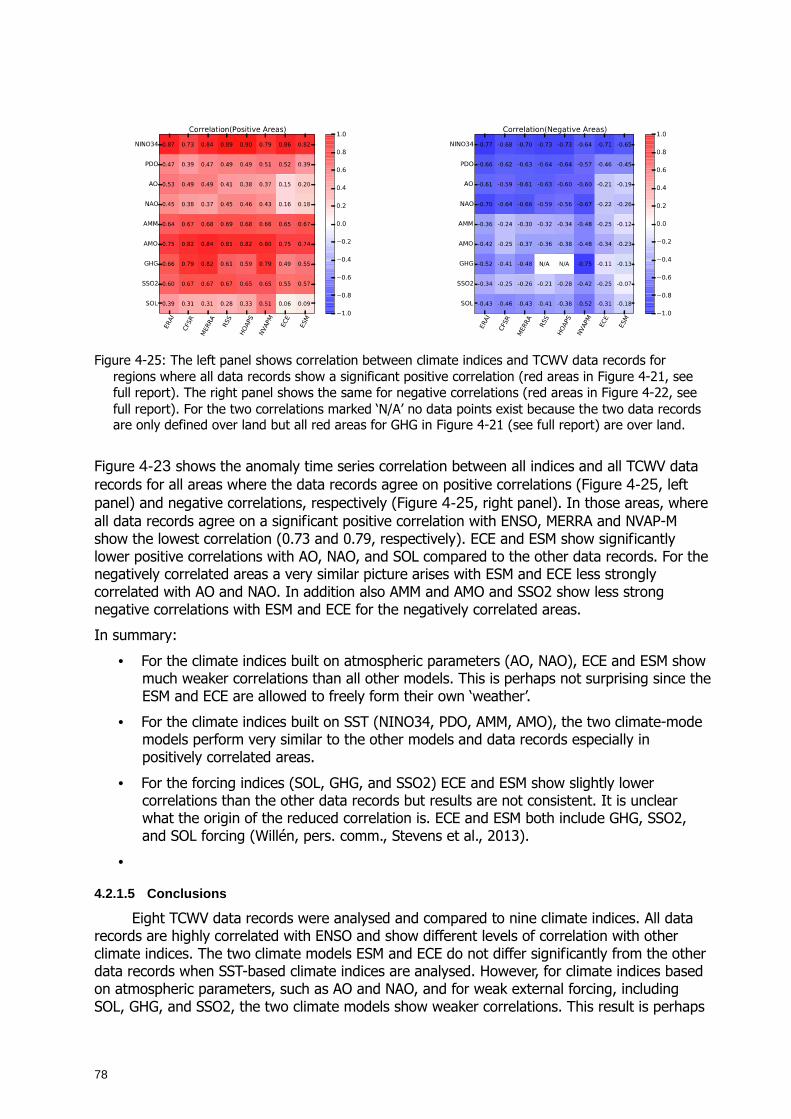
78

Figure 4-25: The left panel shows correlation between climate indices and TCWV data records for regions where all data records show a significant positive correlation (red areas in Figure 4-21, see full report). The right panel shows the same for negative correlations (red areas in Figure 4-22, see full report). For the two correlations marked ‘N/A’ no data points exist because the two data records are only defined over land but all red areas for GHG in Figure 4-21 (see full report) are over land.

Figure 4-23 shows the anomaly time series correlation between all indices and all TCWV data records for all areas where the data records agree on positive correlations (Figure 4-25, left panel) and negative correlations, respectively (Figure 4-25, right panel). In those areas, where all data records agree on a significant positive correlation with ENSO, MERRA and NVAP-M show the lowest correlation (0.73 and 0.79, respectively). ECE and ESM show significantly lower positive correlations with AO, NAO, and SOL compared to the other data records. For the negatively correlated areas a very similar picture arises with ESM and ECE less strongly correlated with AO and NAO. In addition also AMM and AMO and SSO2 show less strong negative correlations with ESM and ECE for the negatively correlated areas.

In summary:

• For the climate indices built on atmospheric parameters (AO, NAO), ECE and ESM show much weaker correlations than all other models. This is perhaps not surprising since the ESM and ECE are allowed to freely form their own ‘weather’.

• For the climate indices built on SST (NINO34, PDO, AMM, AMO), the two climate-mode models perform very similar to the other models and data records especially in positively correlated areas.

• For the forcing indices (SOL, GHG, and SSO2) ECE and ESM show slightly lower correlations than the other data records but results are not consistent. It is unclear what the origin of the reduced correlation is. ECE and ESM both include GHG, SSO2, and SOL forcing (Willén, pers. comm., Stevens et al., 2013).

•

4.2.1.5 Conclusions

Eight TCWV data records were analysed and compared to nine climate indices. All data records are highly correlated with ENSO and show different levels of correlation with other climate indices. The two climate models ESM and ECE do not differ significantly from the other data records when SST-based climate indices are analysed. However, for climate indices based on atmospheric parameters, such as AO and NAO, and for weak external forcing, including SOL, GHG, and SSO2, the two climate models show weaker correlations. This result is perhaps

79

not surprising since all other data records either retrieve or assimilate water vapour information directly and therefore capture not only climate-variability but also weather-related short-term variations, which are not necessarily captured in the climate models.

A large variability of water vapour data records is available and thus an ensemble of satellite based water vapour data records might be considered for e.g. model evaluation. In order to ease analysis and interpretation common features in the ensemble of data records can be identified as e.g. in Figure 4-24. Focusing the subsequent analysis on data from these regions has a large potential to increase confidence in associated results from e.g. model evaluation.

4.2.2 UTH

L. Shi (NOAA), C. J. Schreck III (NOAA, NCSU), M. Schröder (DWD), V. John (EUMETSAT), E.-S. Chung (UM), and B. Soden (UM)

This sub-section examines the variability of several UTH data records. Analyses are carried out to show the variability in a climate context. Several studies have shown that UTH measurements are closely related to large scale circulations and correlated with climate indices (Bates et al., 2001; Chung et al., 2016; Chung et al., 2014; Iacono et al., 2003; Shi and Bates, 2011; Soden et al., 2005). Pairwise correlations are presented in this sub-section to show the variability of UTH in different climate regimes.

4.2.2.1 Data

Three inter-satellite calibrated data records are analysed, including HIRS, AMSU-B/MHS, and METEOSAT MVIRI/SEVIRI UTH. The HIRS UTH data are based on the HIRS Channel 12 climate data record (CDR) version v03r00 (Shi and Bates, 2011) from the National Center for Environmental Information (NCEI). The AMSU-B/MHS (referred to as microwave (MW)) data record (Chung et al., 2013) is from the University of Miami. The METEOSAT UTH data record is MVIRI/SEVIRI version 1 product (Schröder et al., 2014) from the EUMETSAT Satellite Application Facility on Climate Monitoring (CM SAF).

4.2.2.2 Methods

Monthly means of each data record are computed for the time period of each of the data record. Anomalies are analyzed for the METEOSAT domain and selected regions. The one-point (pairwise) correlation maps between satellite UTH and several climate indices, including NINO3.4, PDO, and NAO are computed. The values of the indices are obtained from NOAA Earth System Research Laboratory at http://www.esrl.noaa.gov/psd/data/climateindices/list/). For the correlation analysis the two UTH data records that have more than twenty years of data are analysed, which include the HIRS and the METEOSAT UTH. It has been shown by Chung et al. (2016) that the variability patterns of the MW UTH data record are very similar to the HIRS UTH data record.

4.2.2.3 Results

Time series of anomalies for the three UTH data records over the METEOSAT domain (45°S-45°N, 45°W-45°E) are displayed in Figure 4-27. Though the values of MW UTH, as

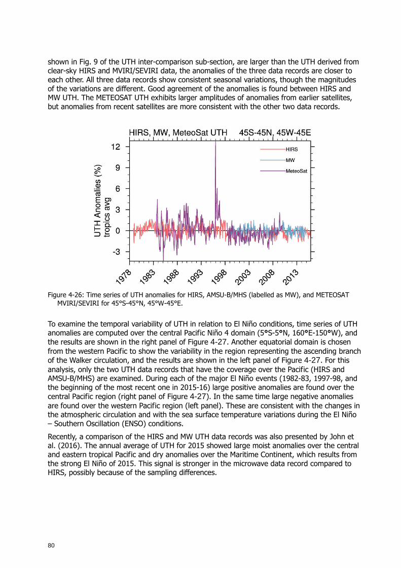
80

shown in Fig. 9 of the UTH inter-comparison sub-section, are larger than the UTH derived from clear-sky HIRS and MVIRI/SEVIRI data, the anomalies of the three data records are closer to each other. All three data records show consistent seasonal variations, though the magnitudes of the variations are different. Good agreement of the anomalies is found between HIRS and MW UTH. The METEOSAT UTH exhibits larger amplitudes of anomalies from earlier satellites, but anomalies from recent satellites are more consistent with the other two data records.

Figure 4-26: Time series of UTH anomalies for HIRS, AMSU-B/MHS (labelled as MW), and METEOSAT

MVIRI/SEVIRI for 45°S-45°N, 45°W-45°E.

To examine the temporal variability of UTH in relation to El Niño conditions, time series of UTH anomalies are computed over the central Pacific Niño 4 domain (5°S-5°N, 160°E-150°W), and the results are shown in the right panel of Figure 4-27. Another equatorial domain is chosen from the western Pacific to show the variability in the region representing the ascending branch of the Walker circulation, and the results are shown in the left panel of Figure 4-27. For this analysis, only the two UTH data records that have the coverage over the Pacific (HIRS and AMSU-B/MHS) are examined. During each of the major El Niño events (1982-83, 1997-98, and the beginning of the most recent one in 2015-16) large positive anomalies are found over the central Pacific region (right panel of Figure 4-27). In the same time large negative anomalies are found over the western Pacific region (left panel). These are consistent with the changes in the atmospheric circulation and with the sea surface temperature variations during the El Niño – Southern Oscillation (ENSO) conditions.

Recently, a comparison of the HIRS and MW UTH data records was also presented by John et al. (2016). The annual average of UTH for 2015 showed large moist anomalies over the central and eastern tropical Pacific and dry anomalies over the Maritime Continent, which results from the strong El Niño of 2015. This signal is stronger in the microwave data record compared to HIRS, possibly because of the sampling differences.

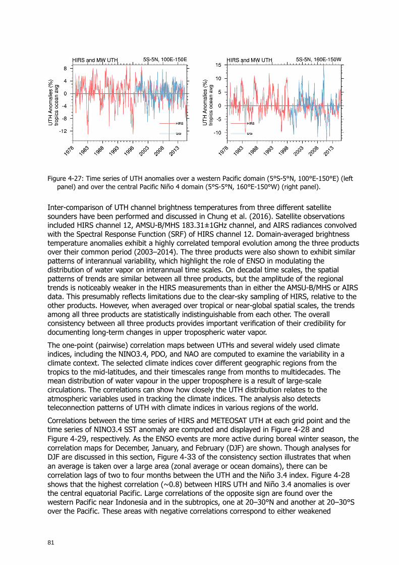
81

Figure 4-27: Time series of UTH anomalies over a western Pacific domain (5°S-5°N, 100°E-150°E) (left panel) and over the central Pacific Niño 4 domain (5°S-5°N, 160°E-150°W) (right panel).

Inter-comparison of UTH channel brightness temperatures from three different satellite sounders have been performed and discussed in Chung et al. (2016). Satellite observations included HIRS channel 12, AMSU-B/MHS 183.31±1GHz channel, and AIRS radiances convolved with the Spectral Response Function (SRF) of HIRS channel 12. Domain-averaged brightness temperature anomalies exhibit a highly correlated temporal evolution among the three products over their common period (2003–2014). The three products were also shown to exhibit similar patterns of interannual variability, which highlight the role of ENSO in modulating the distribution of water vapor on interannual time scales. On decadal time scales, the spatial patterns of trends are similar between all three products, but the amplitude of the regional trends is noticeably weaker in the HIRS measurements than in either the AMSU-B/MHS or AIRS data. This presumably reflects limitations due to the clear-sky sampling of HIRS, relative to the other products. However, when averaged over tropical or near-global spatial scales, the trends among all three products are statistically indistinguishable from each other. The overall consistency between all three products provides important verification of their credibility for documenting long-term changes in upper tropospheric water vapor.

The one-point (pairwise) correlation maps between UTHs and several widely used climate indices, including the NINO3.4, PDO, and NAO are computed to examine the variability in a climate context. The selected climate indices cover different geographic regions from the tropics to the mid-latitudes, and their timescales range from months to multidecades. The mean distribution of water vapour in the upper troposphere is a result of large-scale circulations. The correlations can show how closely the UTH distribution relates to the atmospheric variables used in tracking the climate indices. The analysis also detects teleconnection patterns of UTH with climate indices in various regions of the world.

Correlations between the time series of HIRS and METEOSAT UTH at each grid point and the time series of NINO3.4 SST anomaly are computed and displayed in Figure 4-28 and Figure 4-29, respectively. As the ENSO events are more active during boreal winter season, the correlation maps for December, January, and February (DJF) are shown. Though analyses for DJF are discussed in this section, Figure 4-33 of the consistency section illustrates that when an average is taken over a large area (zonal average or ocean domains), there can be correlation lags of two to four months between the UTH and the Niño 3.4 index. Figure 4-28 shows that the highest correlation (~0.8) between HIRS UTH and Niño 3.4 anomalies is over the central equatorial Pacific. Large correlations of the opposite sign are found over the western Pacific near Indonesia and in the subtropics, one at 20–30°N and another at 20–30°S over the Pacific. These areas with negative correlations correspond to either weakened

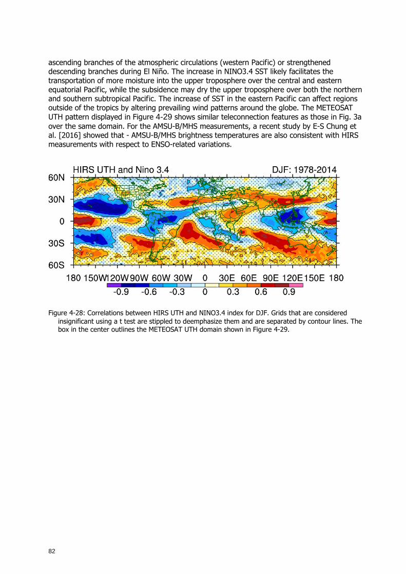
82

ascending branches of the atmospheric circulations (western Pacific) or strengthened descending branches during El Niño. The increase in NINO3.4 SST likely facilitates the transportation of more moisture into the upper troposphere over the central and eastern equatorial Pacific, while the subsidence may dry the upper troposphere over both the northern and southern subtropical Pacific. The increase of SST in the eastern Pacific can affect regions outside of the tropics by altering prevailing wind patterns around the globe. The METEOSAT UTH pattern displayed in Figure 4-29 shows similar teleconnection features as those in Fig. 3a over the same domain. For the AMSU-B/MHS measurements, a recent study by E-S Chung et al. [2016] showed that - AMSU-B/MHS brightness temperatures are also consistent with HIRS measurements with respect to ENSO-related variations.

Figure 4-28: Correlations between HIRS UTH and NINO3.4 index for DJF. Grids that are considered insignificant using a t test are stippled to deemphasize them and are separated by contour lines. The box in the center outlines the METEOSAT UTH domain shown in Figure 4-29.

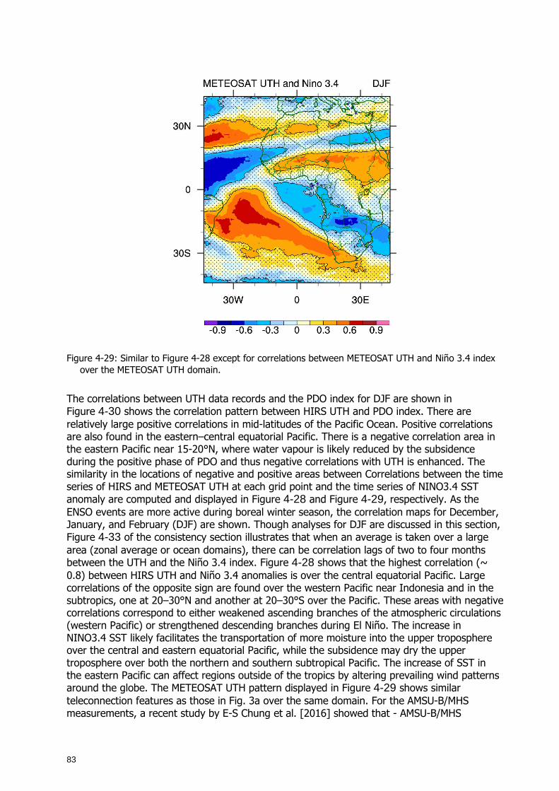
83

Figure 4-29: Similar to Figure 4-28 except for correlations between METEOSAT UTH and Niño 3.4 index over the METEOSAT UTH domain.

The correlations between UTH data records and the PDO index for DJF are shown in Figure 4-30 shows the correlation pattern between HIRS UTH and PDO index. There are relatively large positive correlations in mid-latitudes of the Pacific Ocean. Positive correlations are also found in the eastern–central equatorial Pacific. There is a negative correlation area in the eastern Pacific near 15-20°N, where water vapour is likely reduced by the subsidence during the positive phase of PDO and thus negative correlations with UTH is enhanced. The similarity in the locations of negative and positive areas between Correlations between the time series of HIRS and METEOSAT UTH at each grid point and the time series of NINO3.4 SST anomaly are computed and displayed in Figure 4-28 and Figure 4-29, respectively. As the ENSO events are more active during boreal winter season, the correlation maps for December, January, and February (DJF) are shown. Though analyses for DJF are discussed in this section, Figure 4-33 of the consistency section illustrates that when an average is taken over a large area (zonal average or ocean domains), there can be correlation lags of two to four months between the UTH and the Niño 3.4 index. Figure 4-28 shows that the highest correlation (~ 0.8) between HIRS UTH and Niño 3.4 anomalies is over the central equatorial Pacific. Large correlations of the opposite sign are found over the western Pacific near Indonesia and in the subtropics, one at 20–30°N and another at 20–30°S over the Pacific. These areas with negative correlations correspond to either weakened ascending branches of the atmospheric circulations (western Pacific) or strengthened descending branches during El Niño. The increase in NINO3.4 SST likely facilitates the transportation of more moisture into the upper troposphere over the central and eastern equatorial Pacific, while the subsidence may dry the upper troposphere over both the northern and southern subtropical Pacific. The increase of SST in the eastern Pacific can affect regions outside of the tropics by altering prevailing wind patterns around the globe. The METEOSAT UTH pattern displayed in Figure 4-29 shows similar teleconnection features as those in Fig. 3a over the same domain. For the AMSU-B/MHS measurements, a recent study by E-S Chung et al. [2016] showed that - AMSU-B/MHS

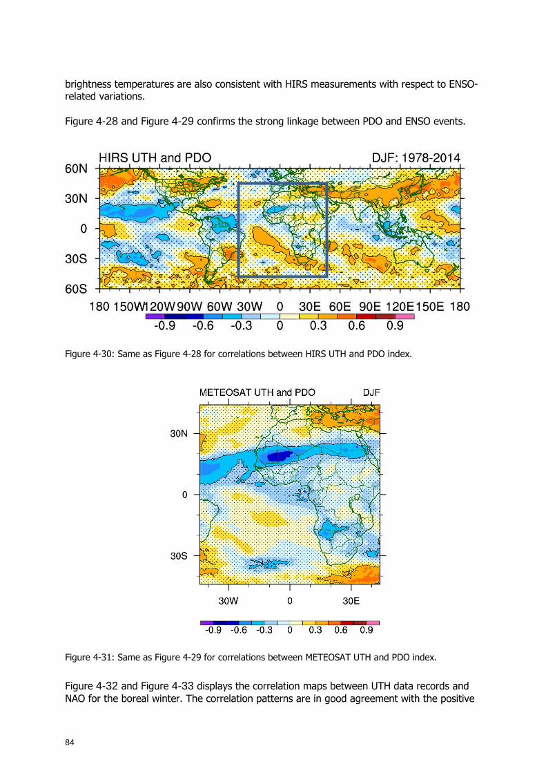
84

brightness temperatures are also consistent with HIRS measurements with respect to ENSO-related variations. Figure 4-28 and Figure 4-29 confirms the strong linkage between PDO and ENSO events.

Figure 4-30: Same as Figure 4-28 for correlations between HIRS UTH and PDO index.

Figure 4-31: Same as Figure 4-29 for correlations between METEOSAT UTH and PDO index.

Figure 4-32 and Figure 4-33 displays the correlation maps between UTH data records and NAO for the boreal winter. The correlation patterns are in good agreement with the positive

85

phase of NAO. High negative correlations are found over the Mediterranean and Europe, while large positive correlations occur over Greenland. Another positive correlation around 15-20°N of the Atlantic is also prominent. During the positive phase when geopotential heights over the subtropical-mid-latitude Atlantic Ocean and western Europe increase, the strengthened atmospheric circulation may create a more favourable condition for transportation of water vapour into the tropical upper troposphere.

Figure 4-32: Same as Figure 4-28 for correlations between HIRS UTH and NAO index.

Figure 4-33: Same as Figure 4-29 for correlations between METEOSAT UTH and NAO index.

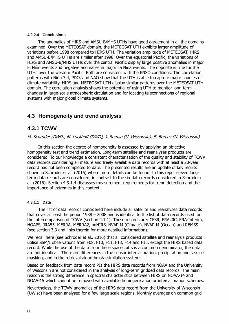
86

4.2.2.4 Conclusions

The anomalies of HIRS and AMSU-B/MHS UTHs have good agreement in all the domains examined. Over the METEOSAT domain, the METEOSAT UTH exhibits larger amplitude of variations before 1998 compared to HIRS UTH. The variation amplitude of METEOSAT, HIRS and AMSU-B/MHS UTHs are similar after 1998. Over the equatorial Pacific, the variations of HIRS and AMSU-B/MHS UTHs over the central Pacific display large positive anomalies in major El Niño events and negative anomalies in major La Niña events. The opposite is true for the UTHs over the western Pacific. Both are consistent with the ENSO conditions. The correlation patterns with Niño 3.4, PDO, and NAO show that the UTH is able to capture major sources of climate variability. HIRS and METEOSAT UTH display similar patterns over the METEOSAT UTH domain. The correlation analysis shows the potential of using UTH to monitor long-term changes in large-scale atmospheric circulation and for locating teleconnections of regional systems with major global climate systems.

4.3 Homogeneity and trend analysis

4.3.1 TCWV

M. Schröder (DWD), M. Lockhoff (DWD), J. Roman (U. Wisconsin), E. Borbas (U. Wisconsin)

In this section the degree of homogeneity is assessed by applying an objective homogeneity test and trend estimation. Long-term satellite and reanalyses products are considered. To our knowledge a consistent characterisation of the quality and stability of TCWV data records considering all mature and freely available data records with at least a 20-year record has not been completed to date. The presented results are an update of key results shown in Schröder et al. (2016) where more details can be found. In this repot eleven long-term data records are considered, in contrast to the six data records considered in Schröder et al. (2016). Section 4.3.1.4 discusses measurement requirements for trend detection and the importance of extremes in this context.

4.3.1.1 Data

The list of data records considered here include all satellite and reanalyses data records that cover at least the period 1988 – 2008 and is identical to the list of data records used for the intercomparison of TCWV (section 4.1.1). These records are: CFSR, ERA20C, ERA-Interim, HOAPS, JRA55, MERRA, MERRA2, nnHIRS, NVAP-M (Climate), NVAP-M (Ocean) and REMSS (see section 3.3 and links therein for more detailed information).

We recall here (see Schröder et al., 2016) that all considered satellite and reanalysis products utilise SSM/I observations from F08, F10, F11, F13, F14 and F15, except the HIRS based data record. While the use of the data from these spacecrafts is a common denominator, the data are not identical. There are differences in the sensor intercalibration, precipitation and sea ice masking, and in the retrieval algorithms/assimilation systems.

Based on feedback from data record PIs the HIRS data records from NOAA and the University of Wisconsin are not considered in the analysis of long-term gridded data records. The main reason is the strong difference in spectral characteristics between HIRS on NOAA-14 and NOAA-15 which cannot be removed with available homogenisation or intercalibration schemes.

Nevertheless, the TCWV anomalies of the HIRS data record from the University of Wisconsin (UWisc) have been analysed for a few large scale regions. Monthly averages on common grid

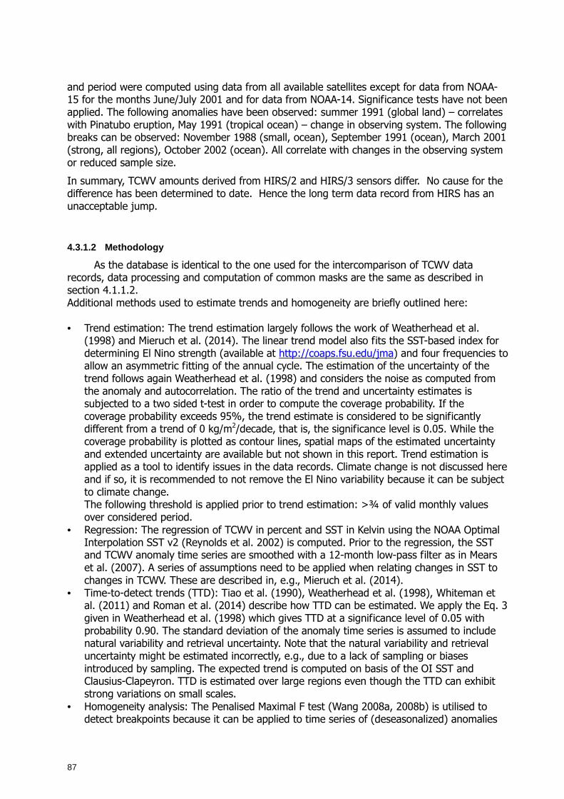
87

and period were computed using data from all available satellites except for data from NOAA-15 for the months June/July 2001 and for data from NOAA-14. Significance tests have not been applied. The following anomalies have been observed: summer 1991 (global land) – correlates with Pinatubo eruption, May 1991 (tropical ocean) – change in observing system. The following breaks can be observed: November 1988 (small, ocean), September 1991 (ocean), March 2001 (strong, all regions), October 2002 (ocean). All correlate with changes in the observing system or reduced sample size.

In summary, TCWV amounts derived from HIRS/2 and HIRS/3 sensors differ. No cause for the difference has been determined to date. Hence the long term data record from HIRS has an unacceptable jump.

4.3.1.2 Methodology

As the database is identical to the one used for the intercomparison of TCWV data records, data processing and computation of common masks are the same as described in section 4.1.1.2. Additional methods used to estimate trends and homogeneity are briefly outlined here: • Trend estimation: The trend estimation largely follows the work of Weatherhead et al.

(1998) and Mieruch et al. (2014). The linear trend model also fits the SST-based index for determining El Nino strength (available at http://coaps.fsu.edu/jma) and four frequencies to allow an asymmetric fitting of the annual cycle. The estimation of the uncertainty of the trend follows again Weatherhead et al. (1998) and considers the noise as computed from the anomaly and autocorrelation. The ratio of the trend and uncertainty estimates is subjected to a two sided t-test in order to compute the coverage probability. If the coverage probability exceeds 95%, the trend estimate is considered to be significantly different from a trend of 0 kg/m2/decade, that is, the significance level is 0.05. While the coverage probability is plotted as contour lines, spatial maps of the estimated uncertainty and extended uncertainty are available but not shown in this report. Trend estimation is applied as a tool to identify issues in the data records. Climate change is not discussed here and if so, it is recommended to not remove the El Nino variability because it can be subject to climate change. The following threshold is applied prior to trend estimation: >¾ of valid monthly values over considered period.

• Regression: The regression of TCWV in percent and SST in Kelvin using the NOAA Optimal Interpolation SST v2 (Reynolds et al. 2002) is computed. Prior to the regression, the SST and TCWV anomaly time series are smoothed with a 12-month low-pass filter as in Mears et al. (2007). A series of assumptions need to be applied when relating changes in SST to changes in TCWV. These are described in, e.g., Mieruch et al. (2014).

• Time-to-detect trends (TTD): Tiao et al. (1990), Weatherhead et al. (1998), Whiteman et al. (2011) and Roman et al. (2014) describe how TTD can be estimated. We apply the Eq. 3 given in Weatherhead et al. (1998) which gives TTD at a significance level of 0.05 with probability 0.90. The standard deviation of the anomaly time series is assumed to include natural variability and retrieval uncertainty. Note that the natural variability and retrieval uncertainty might be estimated incorrectly, e.g., due to a lack of sampling or biases introduced by sampling. The expected trend is computed on basis of the OI SST and Clausius-Clapeyron. TTD is estimated over large regions even though the TTD can exhibit strong variations on small scales.

• Homogeneity analysis: The Penalised Maximal F test (Wang 2008a, 2008b) is utilised to detect breakpoints because it can be applied to time series of (deseasonalized) anomalies

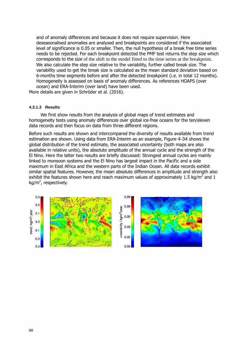
88

and of anomaly differences and because it does not require supervision. Here deseasonalised anomalies are analysed and breakpoints are considered if the associated level of significance is 0.05 or smaller. Then, the null hypothesis of a break free time series needs to be rejected. For each breakpoint detected the PMF test returns the step size which corresponds to the size of the shift in the model fitted to the time series at the breakpoint. We also calculate the step size relative to the variability, further called break size. The variability used to get the break size is calculated as the mean standard deviation based on 6-months time segments before and after the detected breakpoint (i.e. in total 12 months). Homogeneity is assessed on basis of anomaly differences. As references HOAPS (over ocean) and ERA-Interim (over land) have been used.

More details are given in Schröder et al. (2016).

4.3.1.3 Results

We first show results from the analysis of global maps of trend estimates and homogeneity tests using anomaly differences over global ice-free oceans for the ten/eleven data records and then focus on data from three different regions.

Before such results are shown and intercompared the diversity of results available from trend estimation are shown. Using data from ERA-Interim as an example, Figure 4-34 shows the global distribution of the trend estimate, the associated uncertainty (both maps are also available in relative units), the absolute amplitude of the annual cycle and the strength of the El Nino. Here the latter two results are briefly discussed: Strongest annual cycles are mainly linked to monsoon systems and the El Nino has largest impact in the Pacific and a side maximum in East Africa and the western parts of the Indian Ocean. All data records exhibit similar spatial features. However, the mean absolute differences in amplitude and strength also exhibit the features shown here and reach maximum values of approximately 1.5 kg/m2 and 1 kg/m2, respectively.

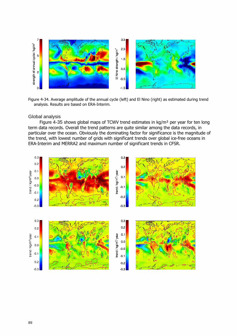
89

Figure 4-34. Average amplitude of the annual cycle (left) and El Nino (right) as estimated during trend

analysis. Results are based on ERA-Interim.

Global analysis Figure 4-35 shows global maps of TCWV trend estimates in kg/m² per year for ten long

term data records. Overall the trend patterns are quite similar among the data records, in particular over the ocean. Obviously the dominating factor for significance is the magnitude of the trend, with lowest number of grids with significant trends over global ice-free oceans in ERA-Interim and MERRA2 and maximum number of significant trends in CFSR.

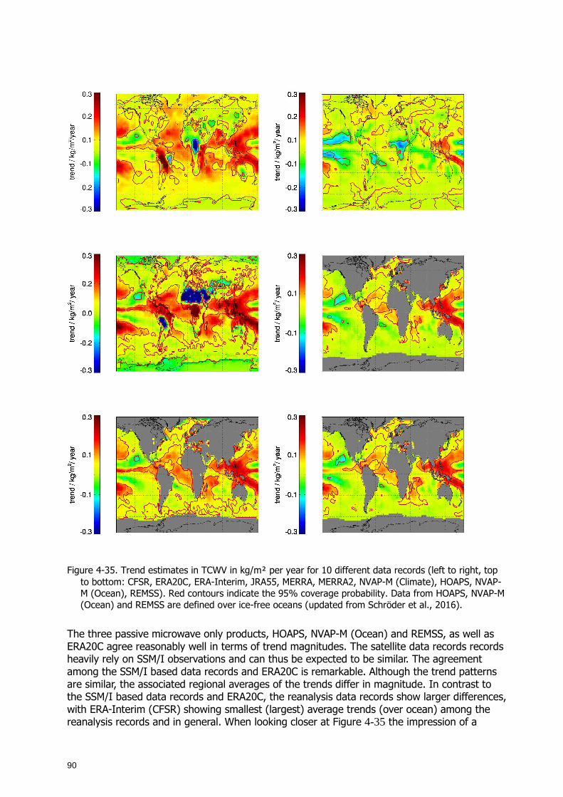
90

Figure 4-35. Trend estimates in TCWV in kg/m² per year for 10 different data records (left to right, top to bottom: CFSR, ERA20C, ERA-Interim, JRA55, MERRA, MERRA2, NVAP-M (Climate), HOAPS, NVAP-M (Ocean), REMSS). Red contours indicate the 95% coverage probability. Data from HOAPS, NVAP-M (Ocean) and REMSS are defined over ice-free oceans (updated from Schröder et al., 2016).

The three passive microwave only products, HOAPS, NVAP-M (Ocean) and REMSS, as well as ERA20C agree reasonably well in terms of trend magnitudes. The satellite data records records heavily rely on SSM/I observations and can thus be expected to be similar. The agreement among the SSM/I based data records and ERA20C is remarkable. Although the trend patterns are similar, the associated regional averages of the trends differ in magnitude. In contrast to the SSM/I based data records and ERA20C, the reanalysis data records show larger differences, with ERA-Interim (CFSR) showing smallest (largest) average trends (over ocean) among the reanalysis records and in general. When looking closer at Figure 4-35 the impression of a

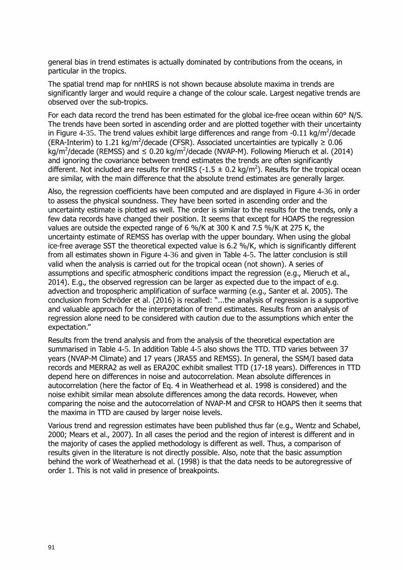
91

general bias in trend estimates is actually dominated by contributions from the oceans, in particular in the tropics.

The spatial trend map for nnHIRS is not shown because absolute maxima in trends are significantly larger and would require a change of the colour scale. Largest negative trends are observed over the sub-tropics.

For each data record the trend has been estimated for the global ice-free ocean within 60° N/S. The trends have been sorted in ascending order and are plotted together with their uncertainty in Figure 4-35. The trend values exhibit large differences and range from -0.11 kg/m2/decade (ERA-Interim) to 1.21 kg/m2/decade (CFSR). Associated uncertainties are typically ≥ 0.06 kg/m2/decade (REMSS) and ≤ 0.20 kg/m2/decade (NVAP-M). Following Mieruch et al. (2014) and ignoring the covariance between trend estimates the trends are often significantly different. Not included are results for nnHIRS (-1.5 ± 0.2 kg/m2). Results for the tropical ocean are similar, with the main difference that the absolute trend estimates are generally larger.

Also, the regression coefficients have been computed and are displayed in Figure 4-36 in order to assess the physical soundness. They have been sorted in ascending order and the uncertainty estimate is plotted as well. The order is similar to the results for the trends, only a few data records have changed their position. It seems that except for HOAPS the regression values are outside the expected range of 6 %/K at 300 K and 7.5 %/K at 275 K, the uncertainty estimate of REMSS has overlap with the upper boundary. When using the global ice-free average SST the theoretical expected value is 6.2 %/K, which is significantly different from all estimates shown in Figure 4-36 and given in Table 4-5. The latter conclusion is still valid when the analysis is carried out for the tropical ocean (not shown). A series of assumptions and specific atmospheric conditions impact the regression (e.g., Mieruch et al., 2014). E.g., the observed regression can be larger as expected due to the impact of e.g. advection and tropospheric amplification of surface warming (e.g., Santer et al. 2005). The conclusion from Schröder et al. (2016) is recalled: “...the analysis of regression is a supportive and valuable approach for the interpretation of trend estimates. Results from an analysis of regression alone need to be considered with caution due to the assumptions which enter the expectation.”

Results from the trend analysis and from the analysis of the theoretical expectation are summarised in Table 4-5. In addition Table 4-5 also shows the TTD. TTD varies between 37 years (NVAP-M Climate) and 17 years (JRA55 and REMSS). In general, the SSM/I based data records and MERRA2 as well as ERA20C exhibit smallest TTD (17-18 years). Differences in TTD depend here on differences in noise and autocorrelation. Mean absolute differences in autocorrelation (here the factor of Eq. 4 in Weatherhead et al. 1998 is considered) and the noise exhibit similar mean absolute differences among the data records. However, when comparing the noise and the autocorrelation of NVAP-M and CFSR to HOAPS then it seems that the maxima in TTD are caused by larger noise levels.

Various trend and regression estimates have been published thus far (e.g., Wentz and Schabel, 2000; Mears et al., 2007). In all cases the period and the region of interest is different and in the majority of cases the applied methodology is different as well. Thus, a comparison of results given in the literature is not directly possible. Also, note that the basic assumption behind the work of Weatherhead et al. (1998) is that the data needs to be autoregressive of order 1. This is not valid in presence of breakpoints.

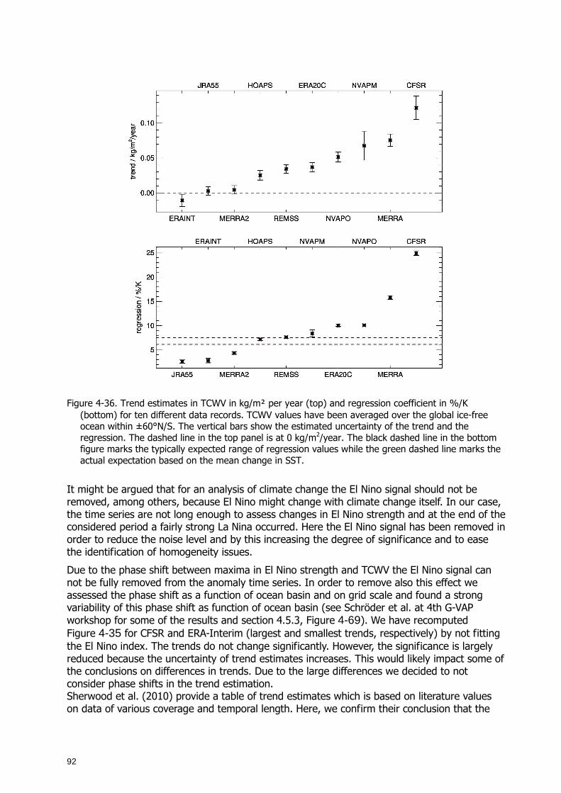
92

Figure 4-36. Trend estimates in TCWV in kg/m² per year (top) and regression coefficient in %/K

(bottom) for ten different data records. TCWV values have been averaged over the global ice-free ocean within ±60°N/S. The vertical bars show the estimated uncertainty of the trend and the regression. The dashed line in the top panel is at 0 kg/m2/year. The black dashed line in the bottom figure marks the typically expected range of regression values while the green dashed line marks the actual expectation based on the mean change in SST.

It might be argued that for an analysis of climate change the El Nino signal should not be removed, among others, because El Nino might change with climate change itself. In our case, the time series are not long enough to assess changes in El Nino strength and at the end of the considered period a fairly strong La Nina occurred. Here the El Nino signal has been removed in order to reduce the noise level and by this increasing the degree of significance and to ease the identification of homogeneity issues.

Due to the phase shift between maxima in El Nino strength and TCWV the El Nino signal can not be fully removed from the anomaly time series. In order to remove also this effect we assessed the phase shift as a function of ocean basin and on grid scale and found a strong variability of this phase shift as function of ocean basin (see Schröder et al. at 4th G-VAP workshop for some of the results and section 4.5.3, Figure 4-69). We have recomputed Figure 4-35 for CFSR and ERA-Interim (largest and smallest trends, respectively) by not fitting the El Nino index. The trends do not change significantly. However, the significance is largely reduced because the uncertainty of trend estimates increases. This would likely impact some of the conclusions on differences in trends. Due to the large differences we decided to not consider phase shifts in the trend estimation. Sherwood et al. (2010) provide a table of trend estimates which is based on literature values on data of various coverage and temporal length. Here, we confirm their conclusion that the

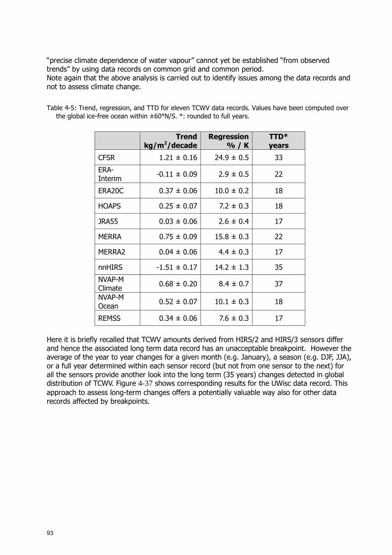
93

“precise climate dependence of water vapour” cannot yet be established “from observed trends” by using data records on common grid and common period. Note again that the above analysis is carried out to identify issues among the data records and not to assess climate change.

Table 4-5: Trend, regression, and TTD for eleven TCWV data records. Values have been computed over the global ice-free ocean within ±60°N/S. *: rounded to full years.

Trend

kg/m2/decade Regression

% / K TTD* years

CFSR 1.21 ± 0.16 24.9 ± 0.5 33

ERA-Interim

-0.11 ± 0.09 2.9 ± 0.5 22

ERA20C 0.37 ± 0.06 10.0 ± 0.2 18

HOAPS 0.25 ± 0.07 7.2 ± 0.3 18

JRA55 0.03 ± 0.06 2.6 ± 0.4 17

MERRA 0.75 ± 0.09 15.8 ± 0.3 22

MERRA2 0.04 ± 0.06 4.4 ± 0.3 17

nnHIRS -1.51 ± 0.17 14.2 ± 1.3 35

NVAP-M Climate

0.68 ± 0.20 8.4 ± 0.7 37

NVAP-M Ocean

0.52 ± 0.07 10.1 ± 0.3 18

REMSS 0.34 ± 0.06 7.6 ± 0.3 17

Here it is briefly recalled that TCWV amounts derived from HIRS/2 and HIRS/3 sensors differ and hence the associated long term data record has an unacceptable breakpoint. However the average of the year to year changes for a given month (e.g. January), a season (e.g. DJF, JJA), or a full year determined within each sensor record (but not from one sensor to the next) for all the sensors provide another look into the long term (35 years) changes detected in global distribution of TCWV. Figure 4-37 shows corresponding results for the UWisc data record. This approach to assess long-term changes offers a potentially valuable way also for other data records affected by breakpoints.

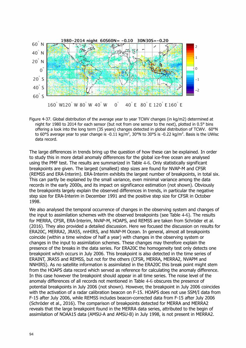
94

Figure 4-37. Global distribution of the average year to year TCWV changes (in kg/m2) determined at night for 1980 to 2014 for each sensor (but not from one sensor to the next), plotted in 0.5° bins offering a look into the long term (35 years) changes detected in global distribution of TCWV. 60°N to 60°S average year to year change is -0.11 kg/m2, 30°N to 30°S is -0.22 kg/m2. Basis is the UWisc data record.

The large differences in trends bring up the question of how these can be explained. In order to study this in more detail anomaly differences for the global ice-free ocean are analysed using the PMF test. The results are summarized in Table 4-6. Only statistically significant breakpoints are given. The largest (smallest) step sizes are found for NVAP-M and CFSR (REMSS and ERA-Interim). ERA-Interim exhibits the largest number of breakpoints, in total six. This can partly be explained by the small variance, even minimal variance among the data records in the early 2000s, and its impact on significance estimation (not shown). Obviously the breakpoints largely explain the observed differences in trends, in particular the negative step size for ERA-Interim in December 1991 and the positive step size for CFSR in October 1998.

We also analysed the temporal occurrence of changes in the observing system and changes of the input to assimilation schemes with the observed breakpoints (see Table 4-6). The results for MERRA, CFSR, ERA-Interim, NVAP-M, HOAPS, and REMSS are taken from Schröder et al. (2016). They also provided a detailed discussion. Here we focused the discussion on results for ERA20C, MERRA2, JRA55, nnHIRS, and NVAP-M Ocean. In general, almost all breakpoints coincide (within a time window of half a year) with changes in the observing system or changes in the input to assimilation schemes. These changes may therefore explain the presence of the breaks in the data series. For ERA20C the homogeneity test only detects one breakpoint which occurs in July 2006. This breakpoint is also detected in the time series of ERAINT, JRA55 and REMSS, but not for the others (CFSR, MERRA, MERRA2, NVAPM and NNHIRS). As no satellite information is assimilated in the ERA20C this break point might stem from the HOAPS data record which served as reference for calculating the anomaly difference. In this case however the breakpoint should appear in all time series. The noise level of the anomaly differences of all records not mentioned in Table 4-6 obscures the presence of potential breakpoints in July 2006 (not shown). However, the breakpoint in July 2006 coincides with the activation of a radar calibration beacon on F-15. HOAPS does not use SSM/I data from F-15 after July 2006, while REMSS includes beacon-corrected data from F-15 after July 2006 (Schröder et al., 2016). The comparison of breakpoints detected for MERRA and MERRA2 reveals that the large breakpoint found in the MERRA data series, attributed to the begin of assimilation of NOAA15 data (AMSU-A and AMSU-B) in July 1998, is not present in MERRA2.

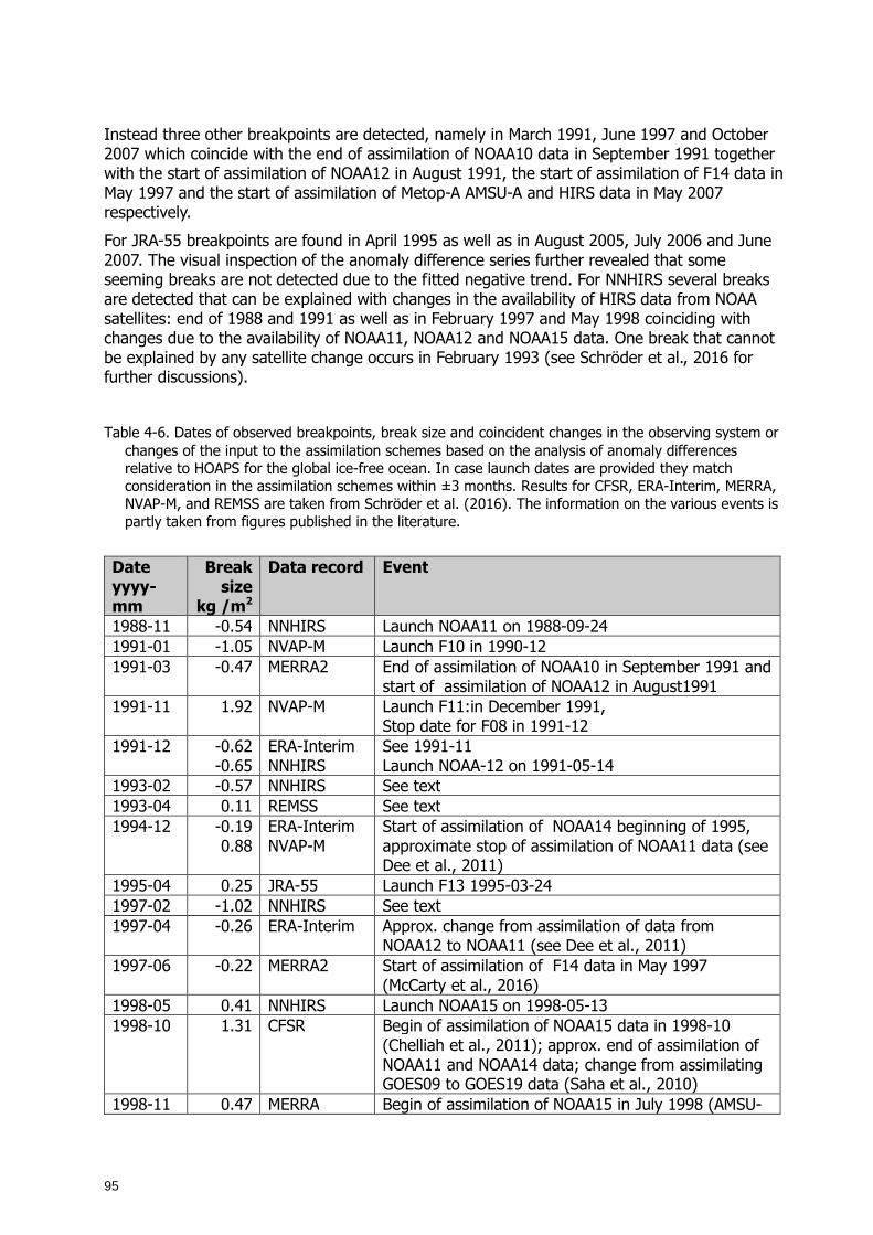
95

Instead three other breakpoints are detected, namely in March 1991, June 1997 and October 2007 which coincide with the end of assimilation of NOAA10 data in September 1991 together with the start of assimilation of NOAA12 in August 1991, the start of assimilation of F14 data in May 1997 and the start of assimilation of Metop-A AMSU-A and HIRS data in May 2007 respectively.

For JRA-55 breakpoints are found in April 1995 as well as in August 2005, July 2006 and June 2007. The visual inspection of the anomaly difference series further revealed that some seeming breaks are not detected due to the fitted negative trend. For NNHIRS several breaks are detected that can be explained with changes in the availability of HIRS data from NOAA satellites: end of 1988 and 1991 as well as in February 1997 and May 1998 coinciding with changes due to the availability of NOAA11, NOAA12 and NOAA15 data. One break that cannot be explained by any satellite change occurs in February 1993 (see Schröder et al., 2016 for further discussions).

Table 4-6. Dates of observed breakpoints, break size and coincident changes in the observing system or changes of the input to the assimilation schemes based on the analysis of anomaly differences relative to HOAPS for the global ice-free ocean. In case launch dates are provided they match consideration in the assimilation schemes within ±3 months. Results for CFSR, ERA-Interim, MERRA, NVAP-M, and REMSS are taken from Schröder et al. (2016). The information on the various events is partly taken from figures published in the literature.

Date yyyy-mm

Break size

kg /m2

Data record Event

1988-11 -0.54 NNHIRS Launch NOAA11 on 1988-09-24 1991-01 -1.05 NVAP-M Launch F10 in 1990-12 1991-03 -0.47 MERRA2 End of assimilation of NOAA10 in September 1991 and

start of assimilation of NOAA12 in August1991 1991-11 1.92 NVAP-M Launch F11:in December 1991,

Stop date for F08 in 1991-12 1991-12 -0.62

-0.65 ERA-Interim NNHIRS

See 1991-11 Launch NOAA-12 on 1991-05-14

1993-02 -0.57 NNHIRS See text 1993-04 0.11 REMSS See text 1994-12 -0.19

0.88 ERA-Interim NVAP-M

Start of assimilation of NOAA14 beginning of 1995, approximate stop of assimilation of NOAA11 data (see Dee et al., 2011)

1995-04 0.25 JRA-55 Launch F13 1995-03-24 1997-02 -1.02 NNHIRS See text 1997-04 -0.26 ERA-Interim Approx. change from assimilation of data from

NOAA12 to NOAA11 (see Dee et al., 2011) 1997-06 -0.22 MERRA2 Start of assimilation of F14 data in May 1997

(McCarty et al., 2016) 1998-05 0.41 NNHIRS Launch NOAA15 on 1998-05-13 1998-10 1.31 CFSR Begin of assimilation of NOAA15 data in 1998-10

(Chelliah et al., 2011); approx. end of assimilation of NOAA11 and NOAA14 data; change from assimilating GOES09 to GOES19 data (Saha et al., 2010)

1998-11 0.47 MERRA Begin of assimilation of NOAA15 in July 1998 (AMSU-

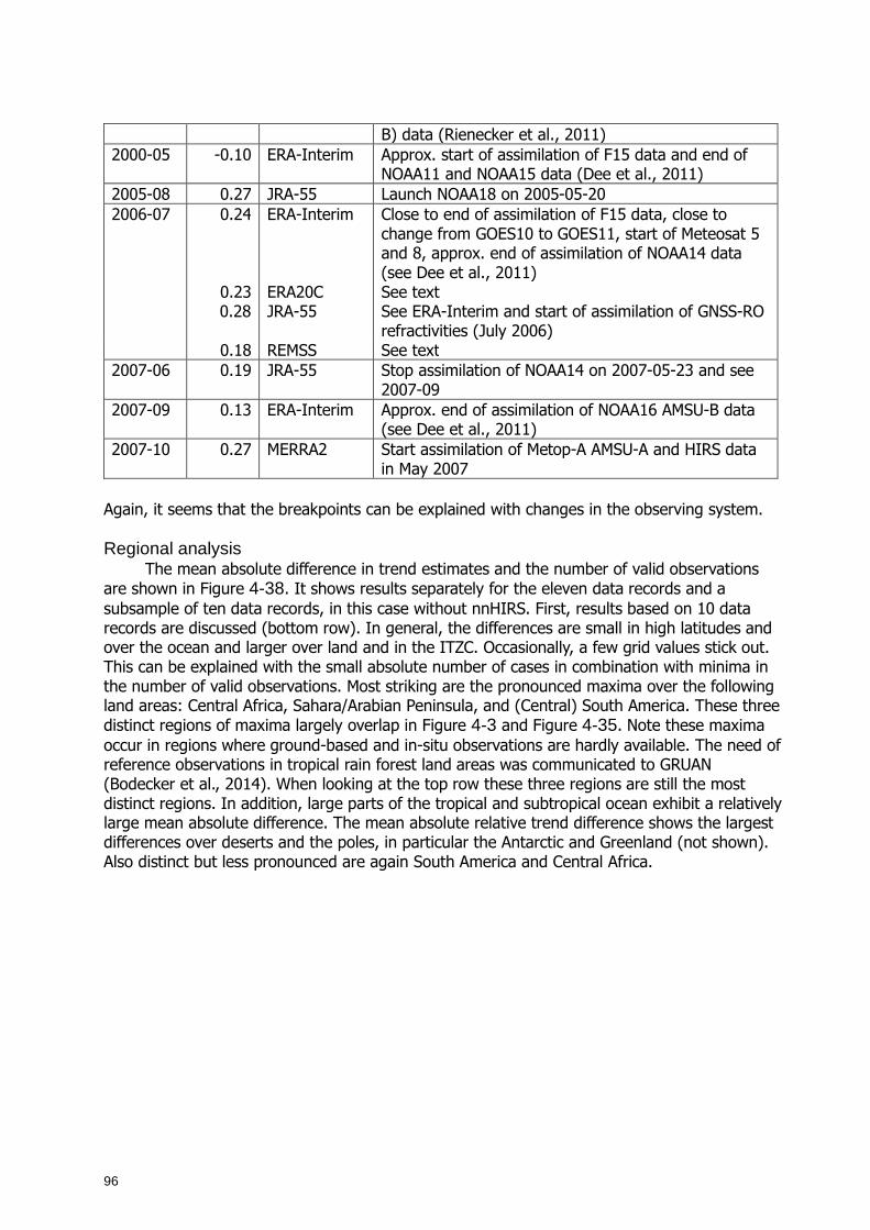
96

B) data (Rienecker et al., 2011) 2000-05 -0.10 ERA-Interim Approx. start of assimilation of F15 data and end of

NOAA11 and NOAA15 data (Dee et al., 2011) 2005-08 0.27 JRA-55 Launch NOAA18 on 2005-05-20 2006-07 0.24

0.23 0.28

ERA-Interim ERA20C JRA-55

Close to end of assimilation of F15 data, close to change from GOES10 to GOES11, start of Meteosat 5 and 8, approx. end of assimilation of NOAA14 data (see Dee et al., 2011) See text See ERA-Interim and start of assimilation of GNSS-RO refractivities (July 2006)

0.18 REMSS See text 2007-06 0.19 JRA-55 Stop assimilation of NOAA14 on 2007-05-23 and see

2007-09 2007-09 0.13 ERA-Interim Approx. end of assimilation of NOAA16 AMSU-B data

(see Dee et al., 2011) 2007-10 0.27 MERRA2 Start assimilation of Metop-A AMSU-A and HIRS data

in May 2007 Again, it seems that the breakpoints can be explained with changes in the observing system. Regional analysis

The mean absolute difference in trend estimates and the number of valid observations are shown in Figure 4-38. It shows results separately for the eleven data records and a subsample of ten data records, in this case without nnHIRS. First, results based on 10 data records are discussed (bottom row). In general, the differences are small in high latitudes and over the ocean and larger over land and in the ITZC. Occasionally, a few grid values stick out. This can be explained with the small absolute number of cases in combination with minima in the number of valid observations. Most striking are the pronounced maxima over the following land areas: Central Africa, Sahara/Arabian Peninsula, and (Central) South America. These three distinct regions of maxima largely overlap in Figure 4-3 and Figure 4-35. Note these maxima occur in regions where ground-based and in-situ observations are hardly available. The need of reference observations in tropical rain forest land areas was communicated to GRUAN (Bodecker et al., 2014). When looking at the top row these three regions are still the most distinct regions. In addition, large parts of the tropical and subtropical ocean exhibit a relatively large mean absolute difference. The mean absolute relative trend difference shows the largest differences over deserts and the poles, in particular the Antarctic and Greenland (not shown). Also distinct but less pronounced are again South America and Central Africa.

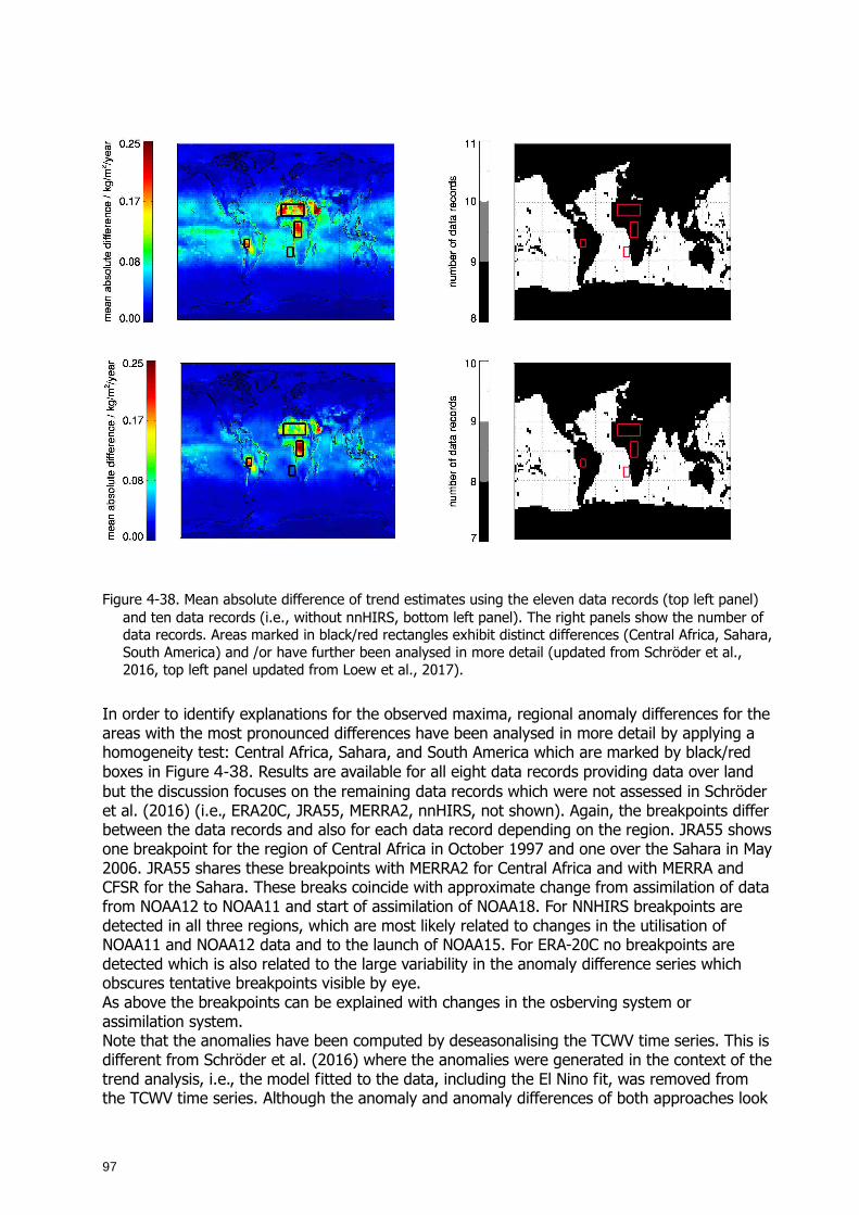
97

Figure 4-38. Mean absolute difference of trend estimates using the eleven data records (top left panel) and ten data records (i.e., without nnHIRS, bottom left panel). The right panels show the number of data records. Areas marked in black/red rectangles exhibit distinct differences (Central Africa, Sahara, South America) and /or have further been analysed in more detail (updated from Schröder et al., 2016, top left panel updated from Loew et al., 2017).

In order to identify explanations for the observed maxima, regional anomaly differences for the areas with the most pronounced differences have been analysed in more detail by applying a homogeneity test: Central Africa, Sahara, and South America which are marked by black/red boxes in Figure 4-38. Results are available for all eight data records providing data over land but the discussion focuses on the remaining data records which were not assessed in Schröder et al. (2016) (i.e., ERA20C, JRA55, MERRA2, nnHIRS, not shown). Again, the breakpoints differ between the data records and also for each data record depending on the region. JRA55 shows one breakpoint for the region of Central Africa in October 1997 and one over the Sahara in May 2006. JRA55 shares these breakpoints with MERRA2 for Central Africa and with MERRA and CFSR for the Sahara. These breaks coincide with approximate change from assimilation of data from NOAA12 to NOAA11 and start of assimilation of NOAA18. For NNHIRS breakpoints are detected in all three regions, which are most likely related to changes in the utilisation of NOAA11 and NOAA12 data and to the launch of NOAA15. For ERA-20C no breakpoints are detected which is also related to the large variability in the anomaly difference series which obscures tentative breakpoints visible by eye. As above the breakpoints can be explained with changes in the osberving system or assimilation system. Note that the anomalies have been computed by deseasonalising the TCWV time series. This is different from Schröder et al. (2016) where the anomalies were generated in the context of the trend analysis, i.e., the model fitted to the data, including the El Nino fit, was removed from the TCWV time series. Although the anomaly and anomaly differences of both approaches look

98

very similar (not shown), a small change in the noise level leads to differences in the detection of breakpoints.

4.3.1.4 Measurement requirements for TCWV trend det ection

In the previous section it was demonstrated that the majority of long-term satellite and reanalyses data records suffer from inhomogeneity issues. An additional aspect is that besides stability aspects also requirements on measurement accuracy exist such that trends in water vapour and more specifically trends in the extremes can be detected.

As greenhouse gas emissions continue to rise, the climate continues to change, altering wind and precipitation patterns and leading to more extreme weather events (IPCC 2014). Global Climate Models (GCMs) provide a way to analyze projected changes in the climate for mitigation decisions. However, the climate is a complex system to emulate leading to high uncertainty in GCMs. Therefore, it is essential to detect predicted TCWV trends with observations on decadal time scales (Wielicki et al. 2013; Ohring and Gruber 1982; Ohring et al. 2005, Tian et al. 2013). Measurement error can severely affect the ability of any sensor to detect a trend in TCWV through instrument noise and algorithm assumptions. Theoretically, the time to detect (TTD) a trend depends on natural variability and measurement error. By including a range of measurement errors in the predicted climate trends we can estimate the effect of measurement error on the TTD a TCWV trend (Wielicki et al. 2013; Leroy et al. 2008; Weatherhead et al. 1998; Whiteman et al. 2011; Roman et al. 2012).

GCM 100-year mean TCWV trends range between 0.055 mm/year and 0.072 mm/year, with largest trends occurring near the equator. Global TCWV TTDs degrade quickly with measurement error; errors higher than 3% result in TTDs above 15 years. Zonal scales require more than 20 years of observations to detect the 100-year TCWV trend with a 5% measurement error. Estimating TCWV trends at regional scales offers a chance to measure statistically significant trends within 10 years with up to a 5% measurement. Furthermore, breaking down the TCWV trends by season can decrease the TTD in some locations, however, some regions with large variability increase the TTD (here after Roman et al. 2014).

Extreme TCWV is a necessary requirement for heavy precipitation and extreme flash flooding events. The potential consequences of extreme TCWV are more severe; it is imperative that our current and future observing system can detect shifts in extreme TCWV within a reasonable number of years. Extreme TCWV (99th percentile) events are expected to increase by a factor of 9 globally by the end of the century. At regional scales, the factor ranges from 5 to 95 depending on the location and season, which has the potential to increase the frequency and intensity of storms, hurricanes, monsoons and Atmospheric Rivers (ARs). The trend in extreme TCWV was 3% per decade, requiring 10 (20) years of TCWV observations with a measurement error less than 3% (5%) (Roman et al., 2015).

In order to exemplary assess the uncertainty of existing observational data record for the extreme percentile the uncertainty of the NASA AIRS version 6 and the EUMETSAT IASI version 6 data records have been analysed using ground-based GPS data from the ARM SGB and TWP site. Roman et al. (2016) shows the uncertainty for AIRS and IASI as a function of PWV (there figures 4 and 5). The fractional error is a function of PWV. The fractional error and thus also the time-to-detect for the extremes is significantly larger than in the 25th-75th percentile range and the error for such cases is mostly larger than 5%.

These results triggered further analysis in order to explain the uncertainty features and to potentially improve the IASI products. It could be shown that an improved handling of surface emissivities reduces the large bias at extreme values.

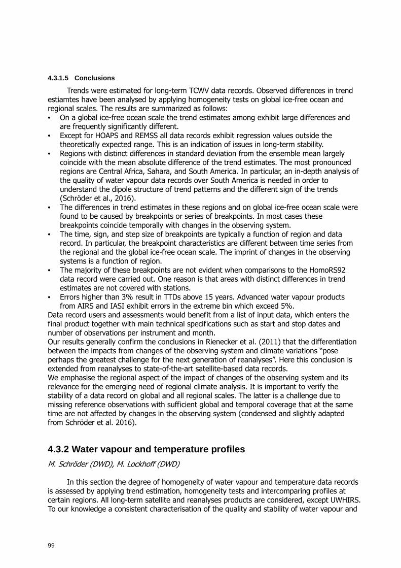
99

4.3.1.5 Conclusions

Trends were estimated for long-term TCWV data records. Observed differences in trend estiamtes have been analysed by applying homogeneity tests on global ice-free ocean and regional scales. The results are summarized as follows: • On a global ice-free ocean scale the trend estimates among exhibit large differences and

are frequently significantly different. • Except for HOAPS and REMSS all data records exhibit regression values outside the

theoretically expected range. This is an indication of issues in long-term stability. • Regions with distinct differences in standard deviation from the ensemble mean largely

coincide with the mean absolute difference of the trend estimates. The most pronounced regions are Central Africa, Sahara, and South America. In particular, an in-depth analysis of the quality of water vapour data records over South America is needed in order to understand the dipole structure of trend patterns and the different sign of the trends (Schröder et al., 2016).

• The differences in trend estimates in these regions and on global ice-free ocean scale were found to be caused by breakpoints or series of breakpoints. In most cases these breakpoints coincide temporally with changes in the observing system.

• The time, sign, and step size of breakpoints are typically a function of region and data record. In particular, the breakpoint characteristics are different between time series from the regional and the global ice-free ocean scale. The imprint of changes in the observing systems is a function of region.

• The majority of these breakpoints are not evident when comparisons to the HomoRS92 data record were carried out. One reason is that areas with distinct differences in trend estimates are not covered with stations.

• Errors higher than 3% result in TTDs above 15 years. Advanced water vapour products from AIRS and IASI exhibit errors in the extreme bin which exceed 5%.

Data record users and assessments would benefit from a list of input data, which enters the final product together with main technical specifications such as start and stop dates and number of observations per instrument and month. Our results generally confirm the conclusions in Rienecker et al. (2011) that the differentiation between the impacts from changes of the observing system and climate variations “pose perhaps the greatest challenge for the next generation of reanalyses”. Here this conclusion is extended from reanalyses to state-of-the-art satellite-based data records. We emphasise the regional aspect of the impact of changes of the observing system and its relevance for the emerging need of regional climate analysis. It is important to verify the stability of a data record on global and all regional scales. The latter is a challenge due to missing reference observations with sufficient global and temporal coverage that at the same time are not affected by changes in the observing system (condensed and slightly adapted from Schröder et al. 2016).

4.3.2 Water vapour and temperature profiles

M. Schröder (DWD), M. Lockhoff (DWD)

In this section the degree of homogeneity of water vapour and temperature data records is assessed by applying trend estimation, homogeneity tests and intercomparing profiles at certain regions. All long-term satellite and reanalyses products are considered, except UWHIRS. To our knowledge a consistent characterisation of the quality and stability of water vapour and

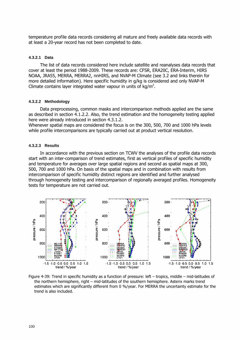
100

temperature profile data records considering all mature and freely available data records with at least a 20-year record has not been completed to date.

4.3.2.1 Data

The list of data records considered here include satellite and reanalyses data records that cover at least the period 1988-2009. These records are: CFSR, ERA20C, ERA-Interim, HIRS NOAA, JRA55, MERRA, MERRA2, nnHIRS, and NVAP-M Climate (see 3.2 and links therein for more detailed information). Here specific humidity in g/kg is considered and only NVAP-M Climate contains layer integrated water vapour in units of kg/m2.

4.3.2.2 Methodology

Data preprocessing, common masks and intercomparison methods applied are the same as described in section 4.1.2.2. Also, the trend estimation and the homogeneity testing applied here were already introduced in section 4.3.1.2. Whenever spatial maps are considered the focus is on the 300, 500, 700 and 1000 hPa levels while profile intercomparisons are typically carried out at product vertical resolution.

4.3.2.3 Results

In accordance with the previous section on TCWV the analyses of the profile data records start with an inter-comparison of trend estimates, first as vertical profiles of specific humidity and temperature for averages over large spatial regions and second as spatial maps at 300, 500, 700 and 1000 hPa. On basis of the spatial maps and in combination with results from intercomparison of specific humidity distinct regions are identified and further analysed through homogeneity testing and intercomparison of regionally averaged profiles. Homogeneity tests for temperature are not carried out.

Figure 4-39: Trend in specific humidity as a function of pressure: left – tropics, middle – mid-latitudes of

the northern hemisphere, right – mid-latitudes of the southern hemisphere. Asterix marks trend estimates which are significantly different from 0 %/year. For MERRA the uncertainty estimate for the trend is also included.

101

Vertical profiles of trend estimates are shown in Figure 4-39. Note that the results for NVAP-M are based on layer integrals and not on specific humidity at a certain level. ERA20C, ERA-Interim, JRA55 and MERRA2 exhibit smallest trends in the middle to lower troposphere in all three cases. Noticeable is that the divergence in trend estimates is larger in the southern than in the northern hemisphere. In the lower troposphere MERRA and CFSR have similar trends and exhibit a side maximum at approximately 800 hPa. Both pairs exhibit significantly (considering the MERRA trend uncertainty) different trends with the CFSR/MERRA trends being larger. In the upper troposphere the overall disagreement is largest. This is particularly true in the tropics where the divergence starts already at approximately 600 hPa. Vertical profiles of trend estimates have also been analysed by Dessler and Davis (2010). Our results are different in detail, also because of differences in temporal coverage, but overall qualitative conclusions are similar. For an analysis of the regression between changes in water vapour and SST we refer to Dessler and Davis (2010).

Figure 4-40: Trend in specific humidity as a function of pressure: left – tropics, middle – mid-latitudes of

the northern hemisphere, right – mid-latitudes of the southern hemisphere. Asterix marks trend estimates which are significantly different from 0 %/year. For MERRA the uncertainty estimate for the trend is also included.

Similar to Figure 4-39 Figure 4-40 shows the trend estimates of temperature profiles from six data records (NVAP-M Climate does not contain temperature). Generally the trends are positive at all levels and regions and slightly increase in the free troposphere with maximum trends around 400 hPa. The latter is also true for the diversity among the data records. Noticeable is that the diversity is smallest over the northern hemisphere. However, several data records exhibit largest positive trends at near surface layers among the three considered regions over the northern hemisphere. Results for nnHIRS generally differ from reanalyses results. The observed features are different from results for specific humidity. Obviously changes in temperature are not the only driver for changes in humidity and dynamical and other physical processes and changes thereof play a role in this context.

102

Figure 4-41: Mean absolute difference of trend estimates using the seven data records: 300, 500, 700

and 1000 hPa clockwise starting top left. Areas marked with rectangles exhibit distinct differences. Grey areas mark elevated terrain which exceeds the considered pressure level.

Figure 4-41 and Figure 4-42 show the mean absolute and relative difference in trend estimates at 300, 500, 700, and 1000 hPa. Regions of maximum differences are stratus (off the coasts of South America and South Africa), Central Africa, Arabian Sea, off the coast of Brazil and South America. Regions of maximum difference are different from the maxima in TCWV, except for maxima at the poles and over Central Africa (verify Figure 4-38 and related discussions). Also the strong land/sea contrast vanishes if not reverses here, with a tendency of maxima in trend differences occurring over the ocean, again except for Central Africa. The analysis is largely based on reanalysis data records. Over ocean ground-truth is hardly available and the assimilation is dominated by satellite data. This might explain to some extend the tendency of larger differences over ocean than over land. Finally, regions of maximum standard deviation and of maxima in trend differences generally do not coincide, except for stratus regions off the coast of South Africa (verify Figure 4-7). This is an indication that in the profile case the differences in trend estimates and maxima in standard deviation might not be caused by breakpoints alone. Occasionally, a few grid values of the spatial maps at 700 and 1000 hPa stick out because minima in the number of valid observations occur at the border of elevated terrain. The differences in trend estimates were also computed for all data records except nnHIRS. The overall results are similar, except for an overall smaller difference in subtropical areas.

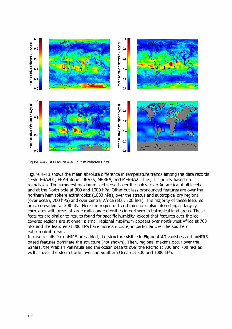
103

Figure 4-42: As Figure 4-41 but in relative units.

Figure 4-43 shows the mean absolute difference in temperature trends among the data records CFSR, ERA20C, ERA-Interim, JRA55, MERRA, and MERRA2. Thus, it is purely based on reanalyses. The strongest maximum is observed over the poles: over Antarctica at all levels and at the North pole at 300 and 1000 hPa. Other but less pronounced features are over the northern hemisphere extratropics (1000 hPa), over the stratus and subtropical dry regions (over ocean, 700 hPa) and over central Africa (500, 700 hPa). The majority of these features are also evident at 300 hPa. Here the region of trend minima is also interesting: it largely correlates with areas of large radiosonde densities in northern extratropical land areas. These features are similar to results found for specific humidity, except that features over the ice covered regions are stronger, a small regional maximum appears over north-west Africa at 700 hPa and the features at 300 hPa have more structure, in particular over the southern extratropical ocean. In case results for nnHIRS are added, the structure visible in Figure 4-43 vanishes and nnHIRS based features dominate the structure (not shown). Then, regional maxima occur over the Sahara, the Arabian Peninsula and the ocean deserts over the Pacific at 300 and 700 hPa as well as over the storm tracks over the Southern Ocean at 500 and 1000 hPa.

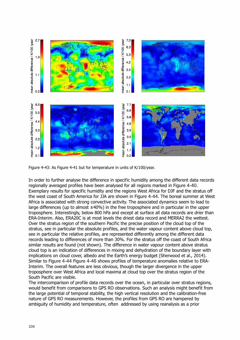
104

Figure 4-43: As Figure 4-41 but for temperature in units of K/100/year.

In order to further analyse the difference in specific humidity among the different data records regionally averaged profiles have been analysed for all regions marked in Figure 4-40. Exemplary results for specific humidity and the regions West Africa for DJF and the stratus off the west coast of South America for JJA are shown in Figure 4-44. The boreal summer at West Africa is associated with strong convective activity. The associated dynamics seem to lead to large differences (up to almost ±40%) in the free troposphere and in particular in the upper troposphere. Interestingly, below 800 hPa and except at surface all data records are drier than ERA-Interim. Also, ERA20C is at most levels the driest data record and MERRA2 the wettest. Over the stratus region of the southern Pacific the precise position of the cloud top of the stratus, see in particular the absolute profiles, and the water vapour content above cloud top, see in particular the relative profiles, are represented differently among the different data records leading to differences of more than 30%. For the stratus off the coast of South Africa similar results are found (not shown). The difference in water vapour content above stratus cloud top is an indication of differences in mixing and dehydration of the boundary layer with implications on cloud cover, albedo and the Earth’s energy budget (Sherwood et al., 2014). Similar to Figure 4-44 Figure 4-46 shows profiles of temperature anomalies relative to ERA-Interim. The overall features are less obvious, though the larger divergence in the upper troposphere over West Africa and local maxima at cloud top over the stratus region of the South Pacific are visible. The intercomparison of profile data records over the ocean, in particular over stratus regions, would benefit from comparisons to GPS RO observations. Such an analysis might benefit from the large potential of temporal stability, the high vertical resolution and the calibration-free nature of GPS RO measurements. However, the profiles from GPS RO are hampered by ambiguity of humidity and temperature, often addressed by using reanalysis as a prior

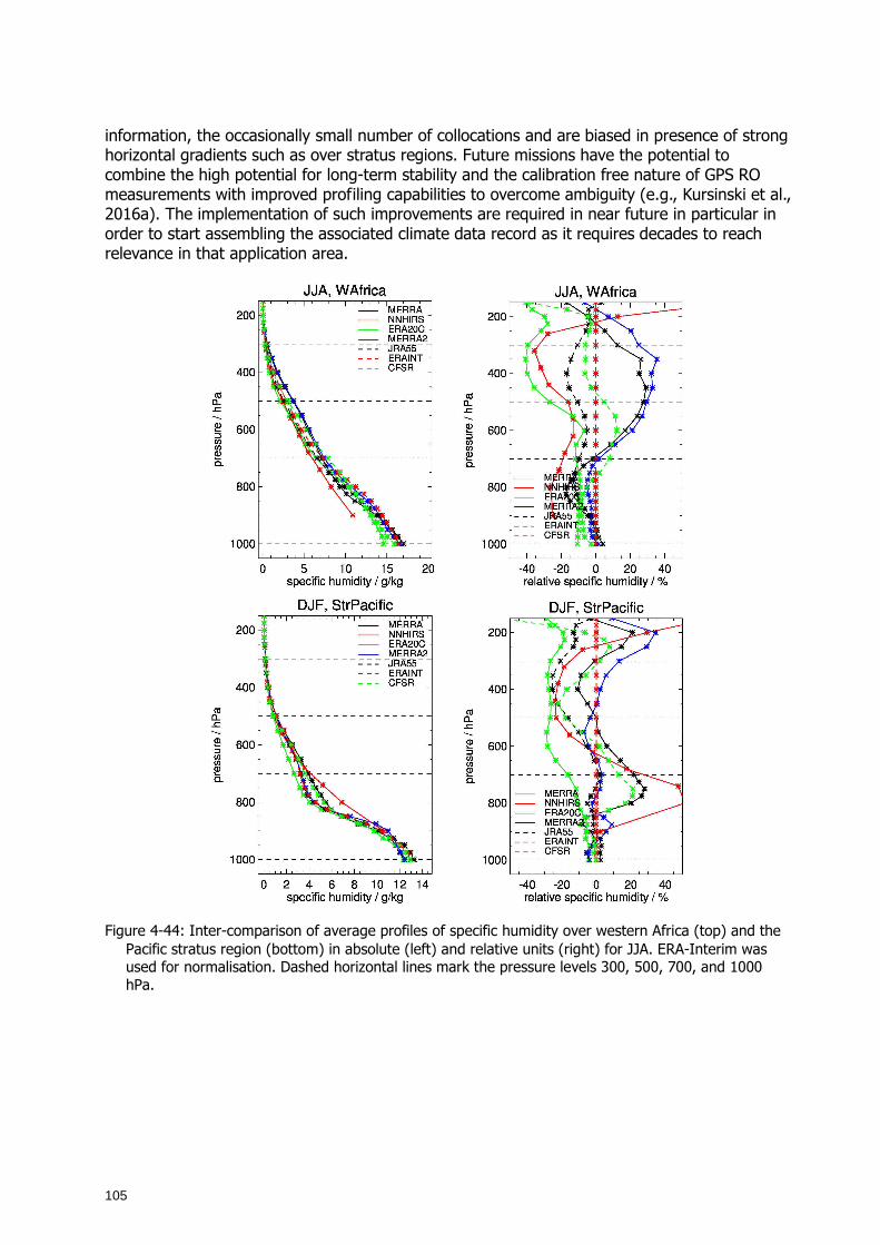
105

information, the occasionally small number of collocations and are biased in presence of strong horizontal gradients such as over stratus regions. Future missions have the potential to combine the high potential for long-term stability and the calibration free nature of GPS RO measurements with improved profiling capabilities to overcome ambiguity (e.g., Kursinski et al., 2016a). The implementation of such improvements are required in near future in particular in order to start assembling the associated climate data record as it requires decades to reach relevance in that application area.

Figure 4-44: Inter-comparison of average profiles of specific humidity over western Africa (top) and the

Pacific stratus region (bottom) in absolute (left) and relative units (right) for JJA. ERA-Interim was used for normalisation. Dashed horizontal lines mark the pressure levels 300, 500, 700, and 1000 hPa.

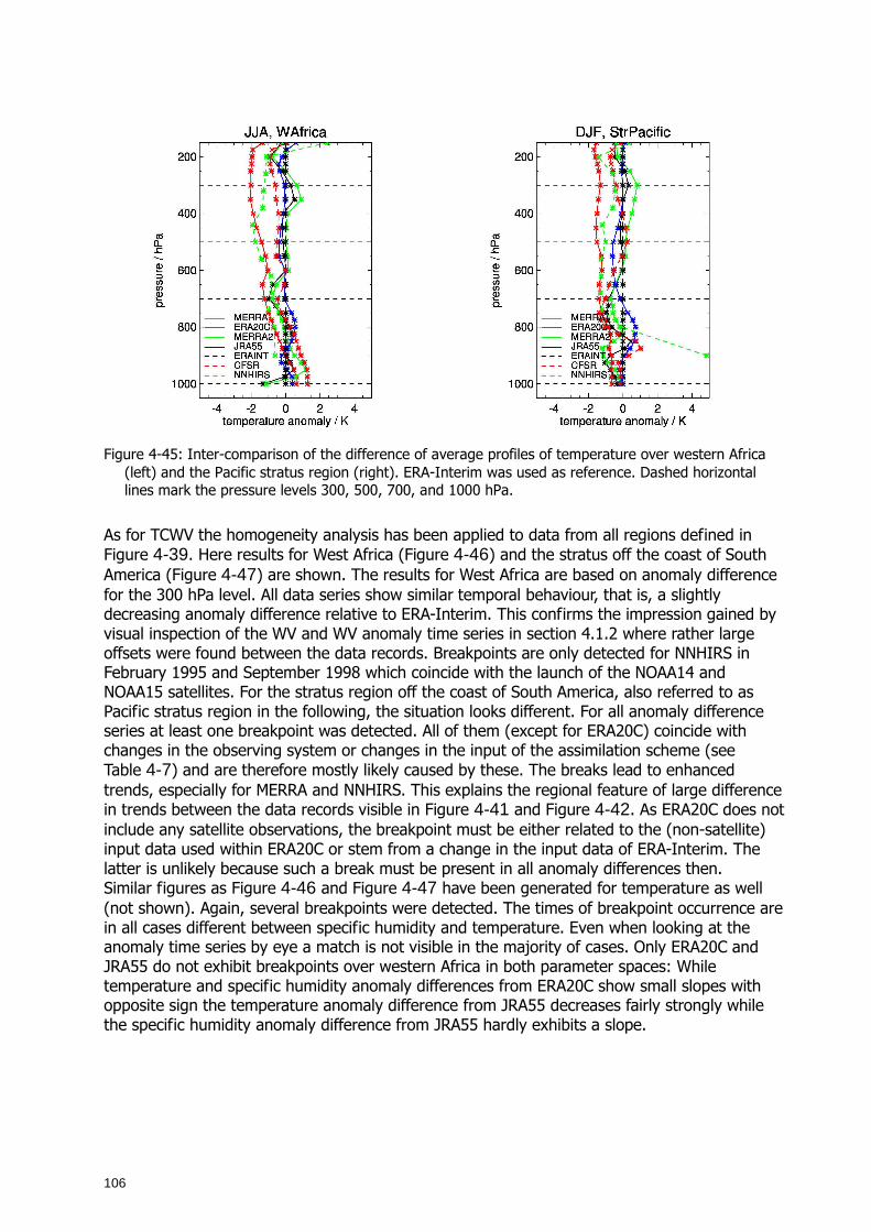
106

Figure 4-45: Inter-comparison of the difference of average profiles of temperature over western Africa

(left) and the Pacific stratus region (right). ERA-Interim was used as reference. Dashed horizontal lines mark the pressure levels 300, 500, 700, and 1000 hPa.

As for TCWV the homogeneity analysis has been applied to data from all regions defined in Figure 4-39. Here results for West Africa (Figure 4-46) and the stratus off the coast of South America (Figure 4-47) are shown. The results for West Africa are based on anomaly difference for the 300 hPa level. All data series show similar temporal behaviour, that is, a slightly decreasing anomaly difference relative to ERA-Interim. This confirms the impression gained by visual inspection of the WV and WV anomaly time series in section 4.1.2 where rather large offsets were found between the data records. Breakpoints are only detected for NNHIRS in February 1995 and September 1998 which coincide with the launch of the NOAA14 and NOAA15 satellites. For the stratus region off the coast of South America, also referred to as Pacific stratus region in the following, the situation looks different. For all anomaly difference series at least one breakpoint was detected. All of them (except for ERA20C) coincide with changes in the observing system or changes in the input of the assimilation scheme (see Table 4-7) and are therefore mostly likely caused by these. The breaks lead to enhanced trends, especially for MERRA and NNHIRS. This explains the regional feature of large difference in trends between the data records visible in Figure 4-41 and Figure 4-42. As ERA20C does not include any satellite observations, the breakpoint must be either related to the (non-satellite) input data used within ERA20C or stem from a change in the input data of ERA-Interim. The latter is unlikely because such a break must be present in all anomaly differences then. Similar figures as Figure 4-46 and Figure 4-47 have been generated for temperature as well (not shown). Again, several breakpoints were detected. The times of breakpoint occurrence are in all cases different between specific humidity and temperature. Even when looking at the anomaly time series by eye a match is not visible in the majority of cases. Only ERA20C and JRA55 do not exhibit breakpoints over western Africa in both parameter spaces: While temperature and specific humidity anomaly differences from ERA20C show small slopes with opposite sign the temperature anomaly difference from JRA55 decreases fairly strongly while the specific humidity anomaly difference from JRA55 hardly exhibits a slope.

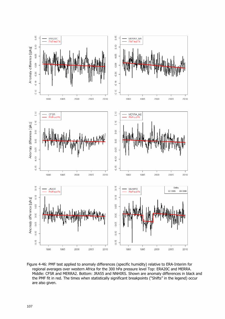
107

Figure 4-46: PMF test applied to anomaly differences (specific humidity) relative to ERA-Interim for regional averages over western Africa for the 300 hPa pressure level Top: ERA20C and MERRA. Middle: CFSR and MERRA2. Bottom: JRA55 and NNHIRS. Shown are anomaly differences in black and the PMF fit in red. The times when statistically significant breakpoints (“Shifts” in the legend) occur are also given.

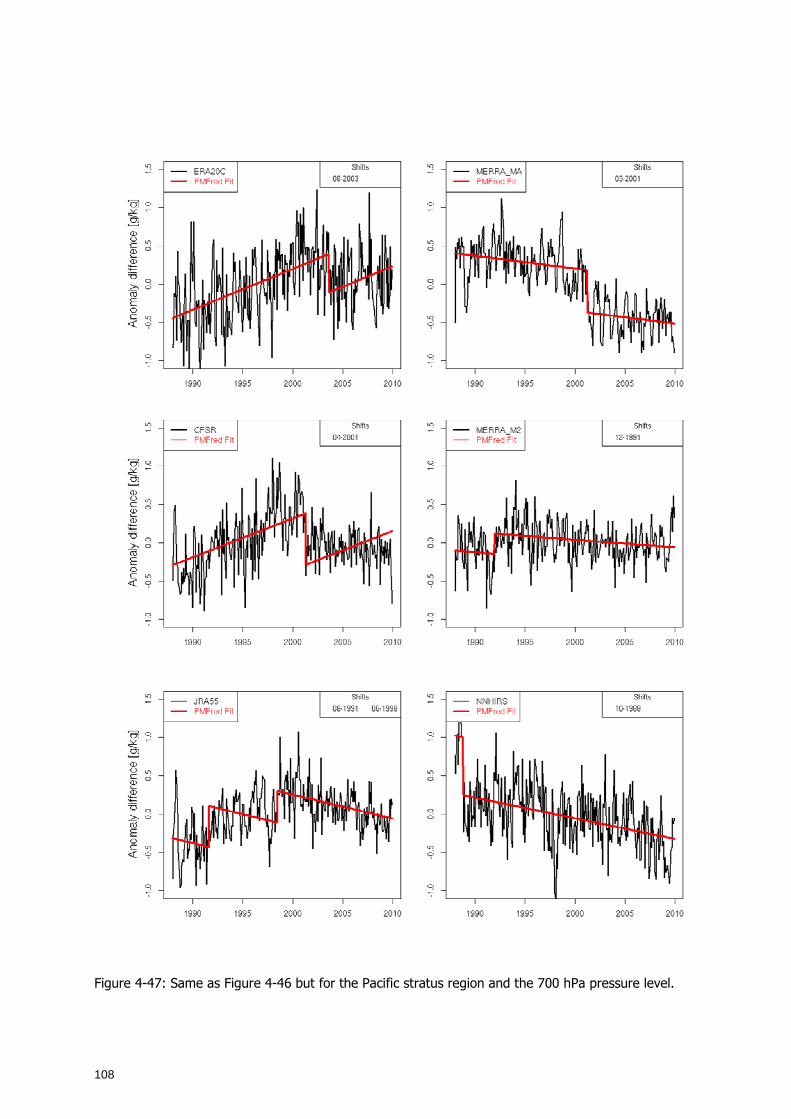
108

Figure 4-47: Same as Figure 4-46 but for the Pacific stratus region and the 700 hPa pressure level.

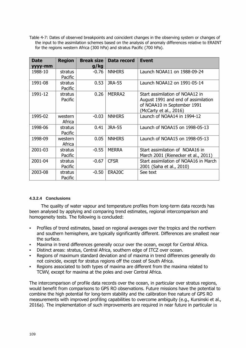
109

Table 4-7: Dates of observed breakpoints and coincident changes in the observing system or changes of the input to the assimilation schemes based on the analysis of anomaly differences relative to ERAINT for the regions western Africa (300 hPa) and stratus Pacific (700 hPa).

Date yyyy-mm

Region Break size g/kg

Data record Event

1988-10 stratus Pacific

-0.76 NNHIRS Launch NOAA11 on 1988-09-24

1991-08 stratus Pacific

0.53 JRA-55 Launch NOAA12 on 1991-05-14

1991-12 stratus Pacific

0.26 MERRA2 Start assimilation of NOAA12 in August 1991 and end of assimilation of NOAA10 in September 1991 (McCarty et al., 2016)

1995-02 western Africa

-0.03 NNHIRS Launch of NOAA14 in 1994-12

1998-06 stratus Pacific

0.41 JRA-55 Launch of NOAA15 on 1998-05-13

1998-09 western Africa

0.05 NNHIRS Launch of NOAA15 on 1998-05-13

2001-03 stratus Pacific

-0.55 MERRA Start assimilation of NOAA16 in March 2001 (Rienecker et al., 2011)

2001-04 stratus Pacific

-0.67 CFSR Start assimilation of NOAA16 in March 2001 (Saha et al., 2010)

2003-08 stratus Pacific

-0.50 ERA20C See text

4.3.2.4 Conclusions

The quality of water vapour and temperature profiles from long-term data records has been analysed by applying and comparing trend estimates, regional intercomparison and homogeneity tests. The following is concluded: • Profiles of trend estimates, based on regional averages over the tropics and the northern

and southern hemisphere, are typically significantly different. Differences are smallest near the surface.

• Maxima in trend differences generally occur over the ocean, except for Central Africa. • Distinct areas: stratus, Central Africa, southern edge of ITCZ over ocean. • Regions of maximum standard deviation and of maxima in trend differences generally do

not coincide, except for stratus regions off the coast of South Africa. • Regions associated to both types of maxima are different from the maxima related to

TCWV, except for maxima at the poles and over Central Africa. The intercomparison of profile data records over the ocean, in particular over stratus regions, would benefit from comparisons to GPS RO observations. Future missions have the potential to combine the high potential for long-term stability and the calibration free nature of GPS RO measurements with improved profiling capabilities to overcome ambiguity (e.g., Kursinski et al., 2016a). The implementation of such improvements are required in near future in particular in

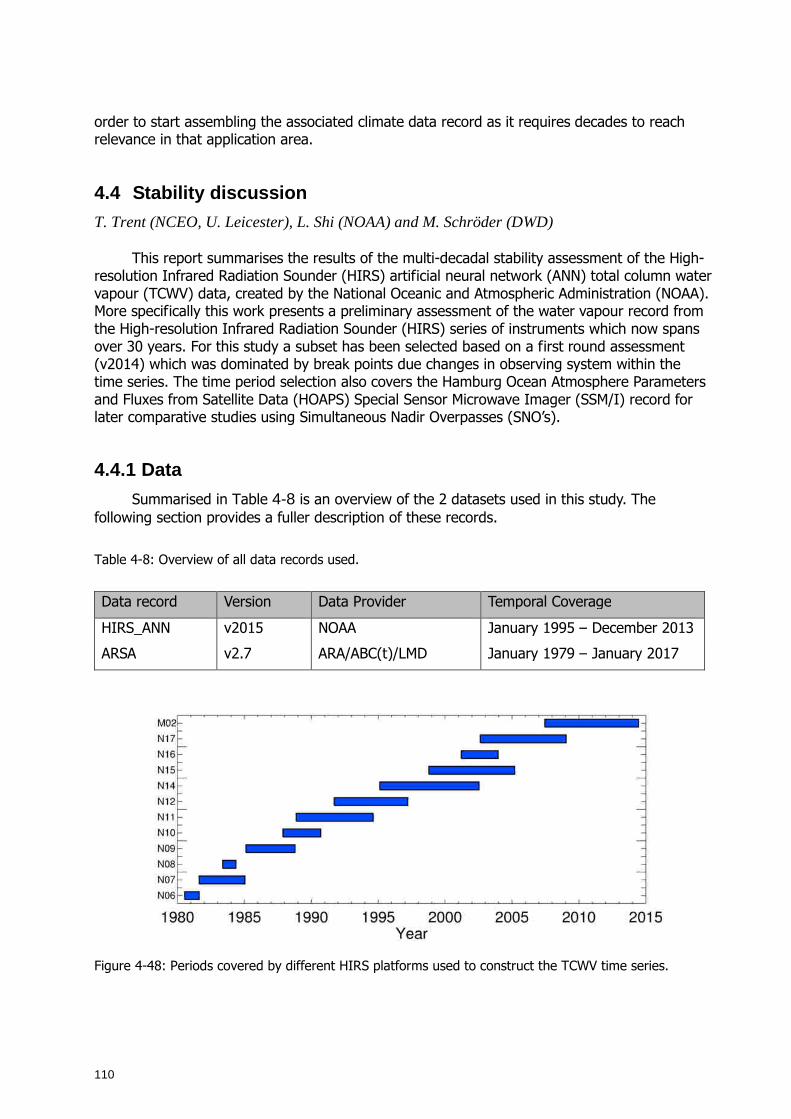
110

order to start assembling the associated climate data record as it requires decades to reach relevance in that application area.

4.4 Stability discussion

T. Trent (NCEO, U. Leicester), L. Shi (NOAA) and M. Schröder (DWD)

This report summarises the results of the multi-decadal stability assessment of the High-resolution Infrared Radiation Sounder (HIRS) artificial neural network (ANN) total column water vapour (TCWV) data, created by the National Oceanic and Atmospheric Administration (NOAA). More specifically this work presents a preliminary assessment of the water vapour record from the High-resolution Infrared Radiation Sounder (HIRS) series of instruments which now spans over 30 years. For this study a subset has been selected based on a first round assessment (v2014) which was dominated by break points due changes in observing system within the time series. The time period selection also covers the Hamburg Ocean Atmosphere Parameters and Fluxes from Satellite Data (HOAPS) Special Sensor Microwave Imager (SSM/I) record for later comparative studies using Simultaneous Nadir Overpasses (SNO’s).

4.4.1 Data

Summarised in Table 4-8 is an overview of the 2 datasets used in this study. The following section provides a fuller description of these records.

Table 4-8: Overview of all data records used.

Data record Version Data Provider Temporal Coverage

HIRS_ANN v2015 NOAA January 1995 – December 2013

ARSA v2.7 ARA/ABC(t)/LMD January 1979 – January 2017

Figure 4-48: Periods covered by different HIRS platforms used to construct the TCWV time series.

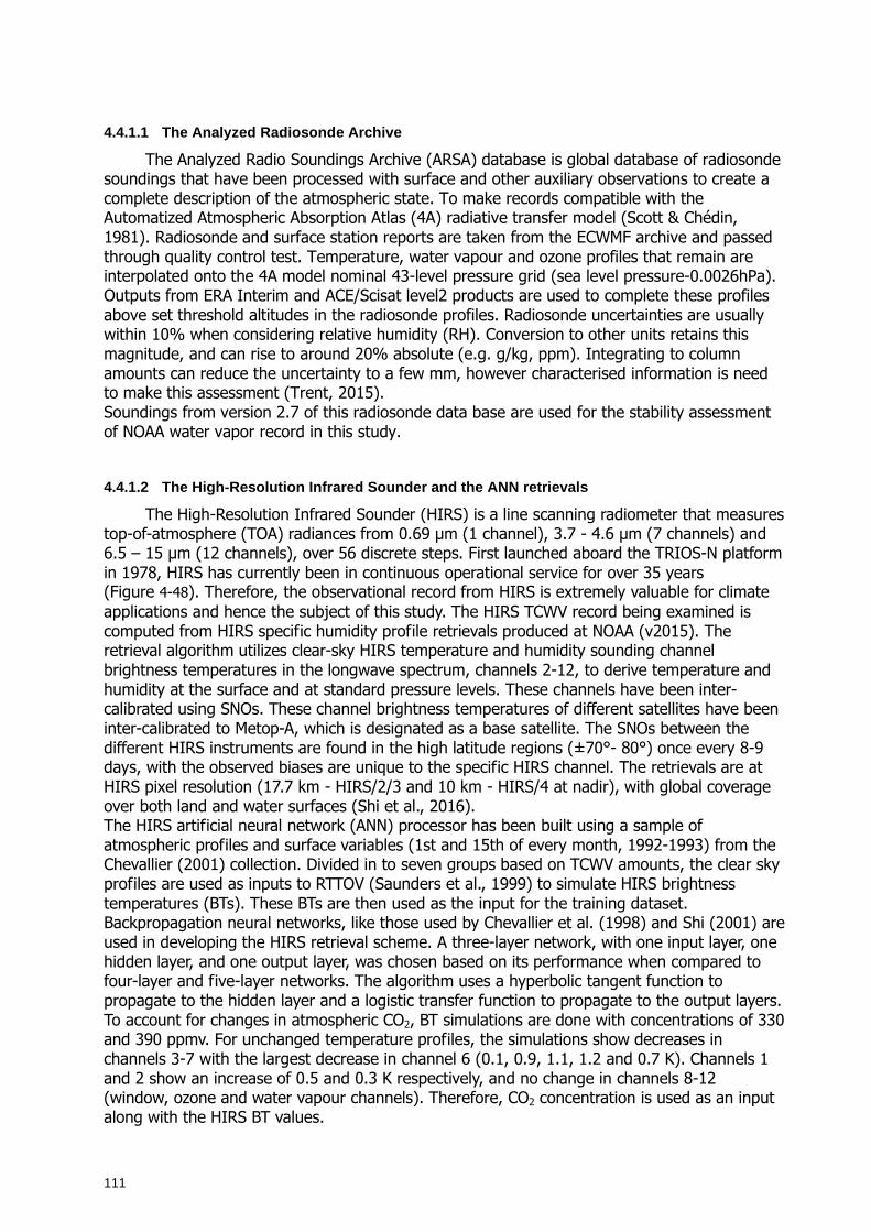
111

4.4.1.1 The Analyzed Radiosonde Archive

The Analyzed Radio Soundings Archive (ARSA) database is global database of radiosonde soundings that have been processed with surface and other auxiliary observations to create a complete description of the atmospheric state. To make records compatible with the Automatized Atmospheric Absorption Atlas (4A) radiative transfer model (Scott & Chédin, 1981). Radiosonde and surface station reports are taken from the ECWMF archive and passed through quality control test. Temperature, water vapour and ozone profiles that remain are interpolated onto the 4A model nominal 43-level pressure grid (sea level pressure-0.0026hPa). Outputs from ERA Interim and ACE/Scisat level2 products are used to complete these profiles above set threshold altitudes in the radiosonde profiles. Radiosonde uncertainties are usually within 10% when considering relative humidity (RH). Conversion to other units retains this magnitude, and can rise to around 20% absolute (e.g. g/kg, ppm). Integrating to column amounts can reduce the uncertainty to a few mm, however characterised information is need to make this assessment (Trent, 2015). Soundings from version 2.7 of this radiosonde data base are used for the stability assessment of NOAA water vapor record in this study.

4.4.1.2 The High-Resolution Infrared Sounder and th e ANN retrievals

The High-Resolution Infrared Sounder (HIRS) is a line scanning radiometer that measures top-of-atmosphere (TOA) radiances from 0.69 µm (1 channel), 3.7 - 4.6 µm (7 channels) and 6.5 – 15 µm (12 channels), over 56 discrete steps. First launched aboard the TRIOS-N platform in 1978, HIRS has currently been in continuous operational service for over 35 years (Figure 4-48). Therefore, the observational record from HIRS is extremely valuable for climate applications and hence the subject of this study. The HIRS TCWV record being examined is computed from HIRS specific humidity profile retrievals produced at NOAA (v2015). The retrieval algorithm utilizes clear-sky HIRS temperature and humidity sounding channel brightness temperatures in the longwave spectrum, channels 2-12, to derive temperature and humidity at the surface and at standard pressure levels. These channels have been inter-calibrated using SNOs. These channel brightness temperatures of different satellites have been inter-calibrated to Metop-A, which is designated as a base satellite. The SNOs between the different HIRS instruments are found in the high latitude regions (±70°- 80°) once every 8-9 days, with the observed biases are unique to the specific HIRS channel. The retrievals are at HIRS pixel resolution (17.7 km - HIRS/2/3 and 10 km - HIRS/4 at nadir), with global coverage over both land and water surfaces (Shi et al., 2016). The HIRS artificial neural network (ANN) processor has been built using a sample of atmospheric profiles and surface variables (1st and 15th of every month, 1992-1993) from the Chevallier (2001) collection. Divided in to seven groups based on TCWV amounts, the clear sky profiles are used as inputs to RTTOV (Saunders et al., 1999) to simulate HIRS brightness temperatures (BTs). These BTs are then used as the input for the training dataset. Backpropagation neural networks, like those used by Chevallier et al. (1998) and Shi (2001) are used in developing the HIRS retrieval scheme. A three-layer network, with one input layer, one hidden layer, and one output layer, was chosen based on its performance when compared to four-layer and five-layer networks. The algorithm uses a hyperbolic tangent function to propagate to the hidden layer and a logistic transfer function to propagate to the output layers. To account for changes in atmospheric CO2, BT simulations are done with concentrations of 330 and 390 ppmv. For unchanged temperature profiles, the simulations show decreases in channels 3-7 with the largest decrease in channel 6 (0.1, 0.9, 1.1, 1.2 and 0.7 K). Channels 1 and 2 show an increase of 0.5 and 0.3 K respectively, and no change in channels 8-12 (window, ozone and water vapour channels). Therefore, CO2 concentration is used as an input along with the HIRS BT values.

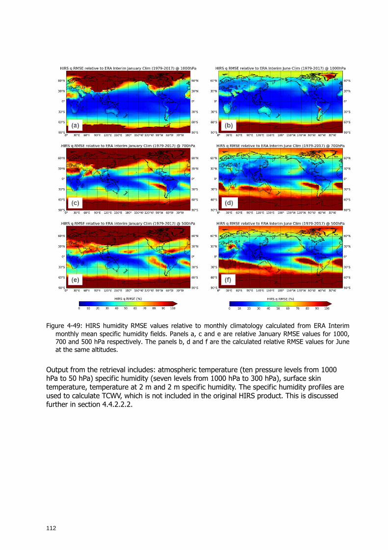
112

Figure 4-49: HIRS humidity RMSE values relative to monthly climatology calculated from ERA Interim monthly mean specific humidity fields. Panels a, c and e are relative January RMSE values for 1000, 700 and 500 hPa respectively. The panels b, d and f are the calculated relative RMSE values for June at the same altitudes.

Output from the retrieval includes: atmospheric temperature (ten pressure levels from 1000 hPa to 50 hPa) specific humidity (seven levels from 1000 hPa to 300 hPa), surface skin temperature, temperature at 2 m and 2 m specific humidity. The specific humidity profiles are used to calculate TCWV, which is not included in the original HIRS product. This is discussed further in section 4.4.2.2.2.

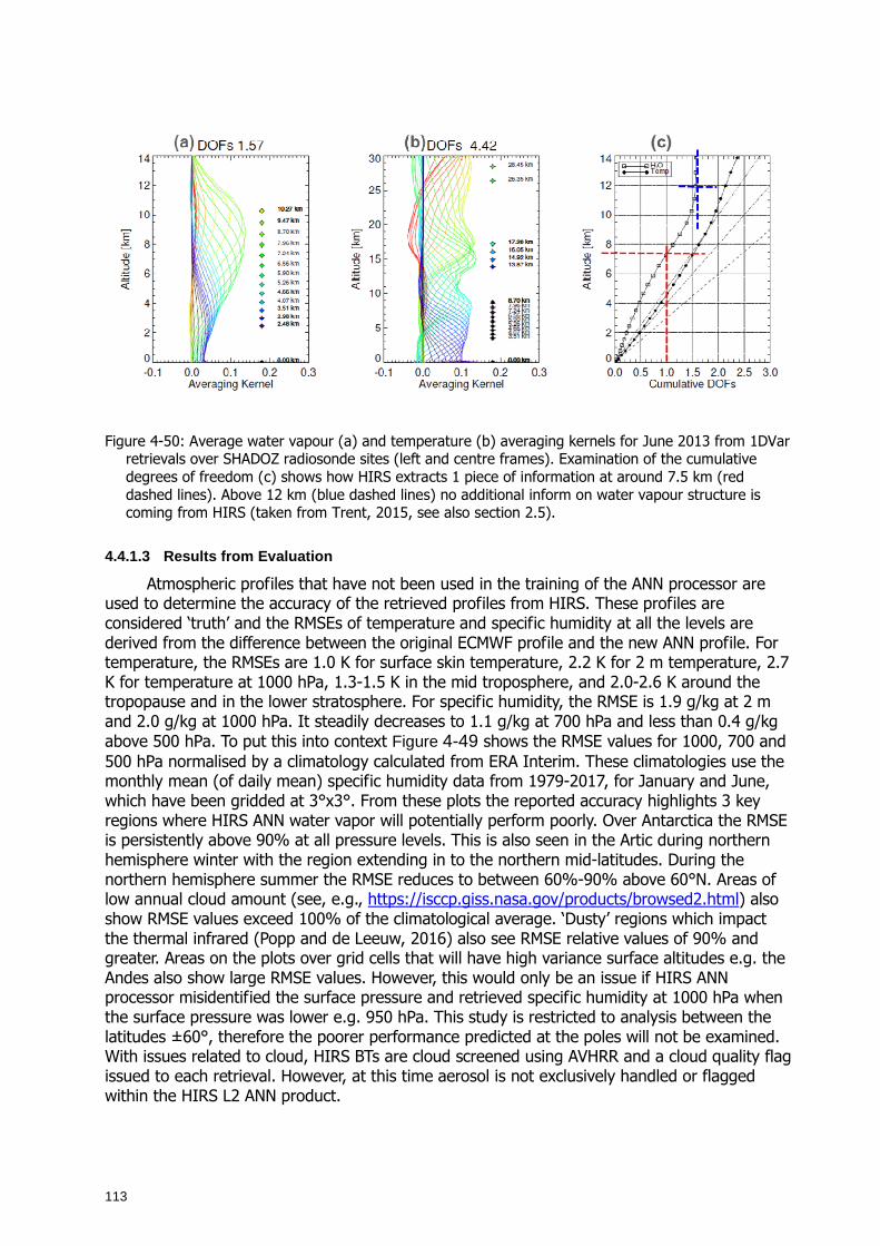
113

Figure 4-50: Average water vapour (a) and temperature (b) averaging kernels for June 2013 from 1DVar retrievals over SHADOZ radiosonde sites (left and centre frames). Examination of the cumulative degrees of freedom (c) shows how HIRS extracts 1 piece of information at around 7.5 km (red dashed lines). Above 12 km (blue dashed lines) no additional inform on water vapour structure is coming from HIRS (taken from Trent, 2015, see also section 2.5).

4.4.1.3 Results from Evaluation

Atmospheric profiles that have not been used in the training of the ANN processor are used to determine the accuracy of the retrieved profiles from HIRS. These profiles are considered ‘truth’ and the RMSEs of temperature and specific humidity at all the levels are derived from the difference between the original ECMWF profile and the new ANN profile. For temperature, the RMSEs are 1.0 K for surface skin temperature, 2.2 K for 2 m temperature, 2.7 K for temperature at 1000 hPa, 1.3-1.5 K in the mid troposphere, and 2.0-2.6 K around the tropopause and in the lower stratosphere. For specific humidity, the RMSE is 1.9 g/kg at 2 m and 2.0 g/kg at 1000 hPa. It steadily decreases to 1.1 g/kg at 700 hPa and less than 0.4 g/kg above 500 hPa. To put this into context Figure 4-49 shows the RMSE values for 1000, 700 and 500 hPa normalised by a climatology calculated from ERA Interim. These climatologies use the monthly mean (of daily mean) specific humidity data from 1979-2017, for January and June, which have been gridded at 3°x3°. From these plots the reported accuracy highlights 3 key regions where HIRS ANN water vapor will potentially perform poorly. Over Antarctica the RMSE is persistently above 90% at all pressure levels. This is also seen in the Artic during northern hemisphere winter with the region extending in to the northern mid-latitudes. During the northern hemisphere summer the RMSE reduces to between 60%-90% above 60°N. Areas of low annual cloud amount (see, e.g., https://isccp.giss.nasa.gov/products/browsed2.html) also show RMSE values exceed 100% of the climatological average. ‘Dusty’ regions which impact the thermal infrared (Popp and de Leeuw, 2016) also see RMSE relative values of 90% and greater. Areas on the plots over grid cells that will have high variance surface altitudes e.g. the Andes also show large RMSE values. However, this would only be an issue if HIRS ANN processor misidentified the surface pressure and retrieved specific humidity at 1000 hPa when the surface pressure was lower e.g. 950 hPa. This study is restricted to analysis between the latitudes ±60°, therefore the poorer performance predicted at the poles will not be examined. With issues related to cloud, HIRS BTs are cloud screened using AVHRR and a cloud quality flag issued to each retrieval. However, at this time aerosol is not exclusively handled or flagged within the HIRS L2 ANN product.

114

These maps provide a guide rather than an explicit description of operational performance. If anything they highlight the lack of robustness in a global RMSE estimate and a possible deficiency in how extremes have been captured in the ANN training dataset. Comparison to other IR sounder retrievals is not easy as the majority of water vapor records do not report uncertainty estimates. However, for sounders that do such IASI or AIRS they report retrieval errors. IASI retrieval error extremes can be around 30-40% (Trent, 2015) while AIRS can reach and exceed 50% (Olsen et al., 2013). With the ERA5 reanalysis (the ECMWF replacement to ERA Interim) a 10 member ensemble estimate is used to produce an estimate of uncertainty (ECMWF spring newsletter 2016, https://tinyurl.com/ybg8tzfe). However, this is a new feature within reanalysis records at this time.

4.4.1.4 Water Vapor Information Content of HIRS

At this point it should be noted that HIRS does not actually retrieve profiles. While the ANN processor produces a profile the vertical sensitivity to HIRS to the troposphere only allows for total column amounts water vapor (TCWV) to be retrieved. Figure 4-50 shows the mean averaging kernels calculated from 1 month of HIRS 1DVar retrievals (Trent, 2015) over SHADOZ tropical radiosonde sites. The averaging kernel shows the sensitivity of the retrieval to the different levels within the atmosphere. A measure of the information content, the total degrees of freedom (DOF) is the sum of the diagonal elements of the averaging kernel. Figure 4-50 3a show that for HIRS the average DOF for tropical regions (where information content will be at its maximum) is 1.64. By examining the cumulative degrees of freedom (CDOF) we can see the vertical sensitivity of the information content (Figure 4-50 c). This figure shows how the first piece of information (CDOF = 1) HIRS can resolve is at around 7.5 km (red dashed lines). The total information content terminates around 12 km (blue dashed lines) where there is no information coming from HIRS within the retrieval and is 100% a priori. Compared to the modern counterparts of HIRS, IASI and AIRS have average DOFs of 5.5 and 4.2 respectively. Therefore, the ANN profiles should be integrated and used as total column water vapour observations instead. A full account of the dataset is discussed in Shi et al. (2016).

4.4.2 Methods

4.4.2.1 Collocation of HIRS with ARSA

For this study profile measurements from ARSA are considered to be collocated with a HIRS observation if they meet the following criteria:

• Fall within ±3 hours of the HIRS observation. • Lie within a 100 km radius of radiosonde launch site in the case of ARSA. • The HIRS cloud flag is equal to 0 or 1 (0 = probability of cloud < 10%, 1= probability of cloud > 10% & < 85%).

Radial distance (d) is calculated using the spherical law of cosines using a constant value of 6371 km for the Earth’s radius. For collocations with ARSA all HIRS IFOV that meet these criteria are used as there is no information on the balloon flight. This approach attempts to increase the signal to noise for differences calculated for each ARSA sounding. Unless otherwise specified all analysis in this study uses collocated HIRS L2 ANN version 2015 (v2015) and ARSA radiosonde humidity profiles.

115

4.4.2.2 Conversion of ARSA Atmospheric Soundings fo r Comparisons with HIRS

Atmospheric temperature and humidity values measured by radiosondes differ from those observed by satellites. While both provide indirect observations (e.g. capacitance which varies as a function of humidity or observed TOA radiances at 6.3 µm), radiosonde measurements are collected on the order of hours opposed the fraction of a second a satellite instrument uses to make an observation. For retrieval schemes that use an optimal estimation (or 1DVar) approach, averaging kernels would be used to smooth the radiosonde profiles to perform ‘like-for-like’ comparisons (Rodgers & Connor, 2003). However, as a neural network scheme has been used to infer profiles temperature and humidity from the HIRS observations averaging kernels are not produced and therefore cannot be employed.

Figure 4-51: Example images of monthly median CIMSS emissivity used for forward model calculation. Clear seasonal differences can be seen between January and June.

Figure 4-52: Conversion of original ARSA temperature and humidity profiles to ARSA_ANN profiles (green and red respectively). The collocated HIRS profiles are over plotted in blue.

In order perform ‘like-for-like’ comparisons between HIRS and ARSA soundings a two-step procedure is used; first HIRS equivalent brightness temperatures (BT_equiv) were calculated using RTTOV (v11) from the ARSA soundings. Secondly, the BT_equiv are passed through the same ANN as the HIRS BT creating the same output found in the HIRS L2 product (section 4.4.1.2).

4.4.2.2.1 Consideration of Emissivity in ARSA conve rsions To increase the description of surface characteristics for RTTOV forward model

simulations a emissivity climatology has been created from the Cooperative Institute for

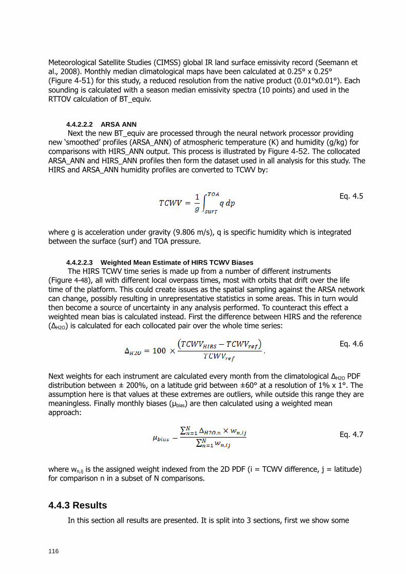
116

Meteorological Satellite Studies (CIMSS) global IR land surface emissivity record (Seemann et al., 2008). Monthly median climatological maps have been calculated at 0.25° x 0.25° (Figure 4-51) for this study, a reduced resolution from the native product (0.01°x0.01°). Each sounding is calculated with a season median emissivity spectra (10 points) and used in the RTTOV calculation of BT_equiv.

4.4.2.2.2 ARSA ANN Next the new BT_equiv are processed through the neural network processor providing

new ‘smoothed’ profiles (ARSA_ANN) of atmospheric temperature (K) and humidity (g/kg) for comparisons with HIRS_ANN output. This process is illustrated by Figure 4-52. The collocated ARSA_ANN and HIRS_ANN profiles then form the dataset used in all analysis for this study. The HIRS and ARSA_ANN humidity profiles are converted to TCWV by:

Eq. 4.5

where g is acceleration under gravity (9.806 m/s), q is specific humidity which is integrated between the surface (surf) and TOA pressure.

4.4.2.2.3 Weighted Mean Estimate of HIRS TCWV Biase s The HIRS TCWV time series is made up from a number of different instruments

(Figure 4-48), all with different local overpass times, most with orbits that drift over the life time of the platform. This could create issues as the spatial sampling against the ARSA network can change, possibly resulting in unrepresentative statistics in some areas. This in turn would then become a source of uncertainty in any analysis performed. To counteract this effect a weighted mean bias is calculated instead. First the difference between HIRS and the reference (∆H2O) is calculated for each collocated pair over the whole time series:

Eq. 4.6

Next weights for each instrument are calculated every month from the climatological ∆H2O PDF distribution between ± 200%, on a latitude grid between ±60° at a resolution of 1% x 1°. The assumption here is that values at these extremes are outliers, while outside this range they are meaningless. Finally monthly biases (µbias) are then calculated using a weighted mean approach:

Eq. 4.7

where wn,ij is the assigned weight indexed from the 2D PDF (i = TCWV difference, j = latitude) for comparison n in a subset of N comparisons.

4.4.3 Results

In this section all results are presented. It is split into 3 sections, first we show some

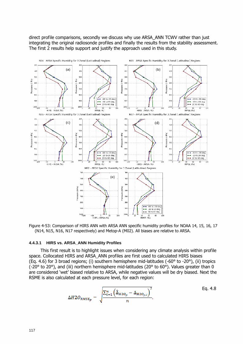
117

direct profile comparisons, secondly we discuss why use ARSA_ANN TCWV rather than just integrating the original radiosonde profiles and finally the results from the stability assessment. The first 2 results help support and justify the approach used in this study.

Figure 4-53: Comparison of HIRS ANN with ARSA ANN specific humidity profiles for NOAA 14, 15, 16, 17

(N14, N15, N16, N17 respectively) and Metop-A (M02). All biases are relative to ARSA.

4.4.3.1 HIRS vs. ARSA_ANN Humidity Profiles

This first result is to highlight issues when considering any climate analysis within profile space. Collocated HIRS and ARSA_ANN profiles are first used to calculated HIRS biases (Eq. 4.6) for 3 broad regions; (i) southern hemisphere mid-latitudes (-60° to -20°), (ii) tropics (-20° to 20°), and (iii) northern hemisphere mid-latitudes (20° to 60°). Values greater than 0 are considered ‘wet’ biased relative to ARSA, while negative values will be dry biased. Next the RSME is also calculated at each pressure level, for each region:

Eq. 4.8

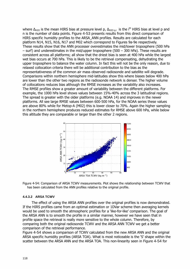
118

where ∆H2O is the mean HIRS bias at pressure level p, ∆H2O p,i is the ith HIRS bias at level p and n is the number of data points. Figure 4-53 presents results from this direct comparison of HIRS specific humidity profiles to the ARSA_ANN profiles. Results are calculated for each platform N14, N15, N16, N17 and M02 which correspond to Figures 9a-9e respectively. These results show that the ANN processer overestimates the mid/lower troposphere (500 hPa – surf) and underestimates in the mid/upper troposphere (500 – 300 hPa). These results are consistent across all platforms; all show that the driest bias is seen at 400 hPa while the largest wet bias occurs at 700 hPa. This is likely to be the retrieval compensating, dehydrating the upper troposphere to balance the water column. In fact this will not be the only reason, due to relaxed collocation criteria there will be additional contribution to the bias as the representativeness of the common air mass observed radiosonde and satellite will degrade. Comparisons within northern hemisphere mid-latitudes show this where biases below 400 hPa are lower than the other two regions as the radiosonde network is denser. The higher volume of collocations reduces bias although the RMSE increases as the variability also increases. The RMSE profiles show a greater amount of variability between the different platforms. For example, the 1000 hPa level shows values between 15%-40% across the 3 latitudinal regions. The spread is greater with the older platforms (e.g. NOAA 14) and improves in the newer platforms. All see large RMSE values between 600-500 hPa, for the NOAA series these values are above 80% while for Metop-A (M02) this is lower closer to 70%. Again the higher sampling in the northern hemisphere produces reduced estimates for RMSE above 600 hPa, while below this altitude they are comparable or larger than the other 2 regions.

Figure 4-54: Comparison of ARSA TCWV measurements. Plot shows the relationship between TCWV that

has been calculated from the ANN profiles relative to the original profile.

4.4.3.2 ARSA TCWV

The effect of using the ARSA ANN profiles over the original profiles is now demonstrated. If the HIRS profiles came from an optimal estimation or 1DVar scheme then averaging kernels would be used to smooth the atmospheric profiles for a ‘like-for-like’ comparison. The goal of the ARSA ANN is to smooth the profile in a similar manner, however we have seen that in profile space the retrieval is really more sensitive to the whole column. Therefore, by comparing both the original radiosonde TCWV and the ARSA ANN TCWV we get a better comparison of the retrieval performance. Figure 4-54 shows a comparison of TCWV calculated from the new ARSA ANN and the original ARSA specific humidity profiles (ARSA TOA). What is most noticeable is the ‘S’ shape within the scatter between the ARSA ANN and the ARSA TOA. This non-linearity seen in Figure 4-54 for

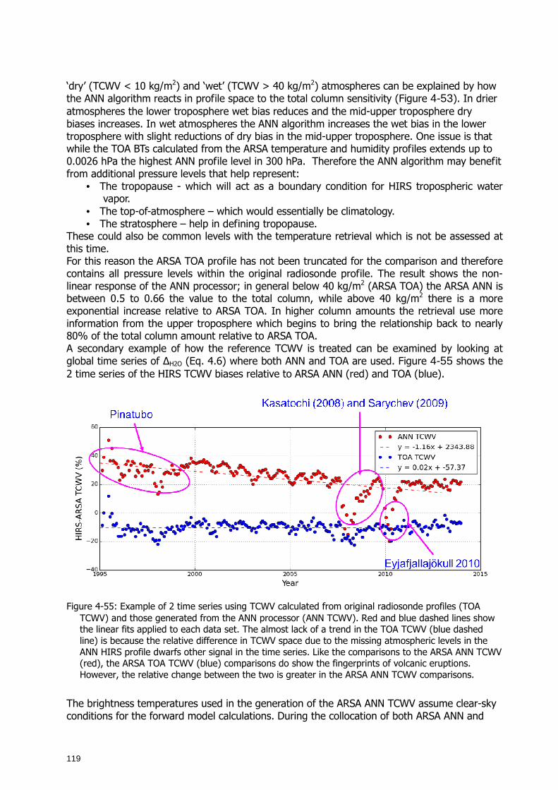
119

‘dry’ (TCWV < 10 kg/m2) and ‘wet’ (TCWV > 40 kg/m2) atmospheres can be explained by how the ANN algorithm reacts in profile space to the total column sensitivity (Figure 4-53). In drier atmospheres the lower troposphere wet bias reduces and the mid-upper troposphere dry biases increases. In wet atmospheres the ANN algorithm increases the wet bias in the lower troposphere with slight reductions of dry bias in the mid-upper troposphere. One issue is that while the TOA BTs calculated from the ARSA temperature and humidity profiles extends up to 0.0026 hPa the highest ANN profile level in 300 hPa. Therefore the ANN algorithm may benefit from additional pressure levels that help represent:

• The tropopause - which will act as a boundary condition for HIRS tropospheric water vapor.

• The top-of-atmosphere – which would essentially be climatology. • The stratosphere – help in defining tropopause.

These could also be common levels with the temperature retrieval which is not be assessed at this time. For this reason the ARSA TOA profile has not been truncated for the comparison and therefore contains all pressure levels within the original radiosonde profile. The result shows the non-linear response of the ANN processor; in general below 40 kg/m2 (ARSA TOA) the ARSA ANN is between 0.5 to 0.66 the value to the total column, while above 40 kg/m2 there is a more exponential increase relative to ARSA TOA. In higher column amounts the retrieval use more information from the upper troposphere which begins to bring the relationship back to nearly 80% of the total column amount relative to ARSA TOA. A secondary example of how the reference TCWV is treated can be examined by looking at global time series of ∆H2O (Eq. 4.6) where both ANN and TOA are used. Figure 4-55 shows the 2 time series of the HIRS TCWV biases relative to ARSA ANN (red) and TOA (blue).

Figure 4-55: Example of 2 time series using TCWV calculated from original radiosonde profiles (TOA

TCWV) and those generated from the ANN processor (ANN TCWV). Red and blue dashed lines show the linear fits applied to each data set. The almost lack of a trend in the TOA TCWV (blue dashed line) is because the relative difference in TCWV space due to the missing atmospheric levels in the ANN HIRS profile dwarfs other signal in the time series. Like the comparisons to the ARSA ANN TCWV (red), the ARSA TOA TCWV (blue) comparisons do show the fingerprints of volcanic eruptions. However, the relative change between the two is greater in the ARSA ANN TCWV comparisons.

The brightness temperatures used in the generation of the ARSA ANN TCWV assume clear-sky conditions for the forward model calculations. During the collocation of both ARSA ANN and

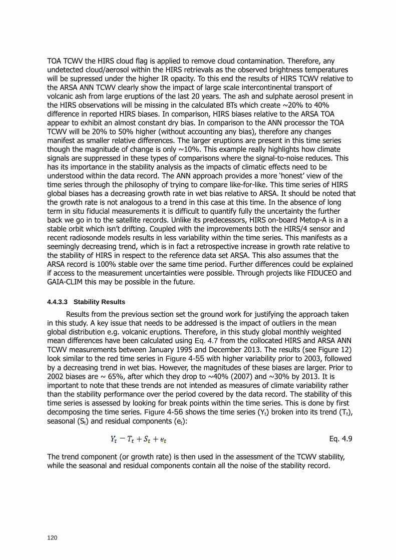
120

TOA TCWV the HIRS cloud flag is applied to remove cloud contamination. Therefore, any undetected cloud/aerosol within the HIRS retrievals as the observed brightness temperatures will be supressed under the higher IR opacity. To this end the results of HIRS TCWV relative to the ARSA ANN TCWV clearly show the impact of large scale intercontinental transport of volcanic ash from large eruptions of the last 20 years. The ash and sulphate aerosol present in the HIRS observations will be missing in the calculated BTs which create ~20% to 40% difference in reported HIRS biases. In comparison, HIRS biases relative to the ARSA TOA appear to exhibit an almost constant dry bias. In comparison to the ANN processor the TOA TCWV will be 20% to 50% higher (without accounting any bias), therefore any changes manifest as smaller relative differences. The larger eruptions are present in this time series though the magnitude of change is only ~10%. This example really highlights how climate signals are suppressed in these types of comparisons where the signal-to-noise reduces. This has its importance in the stability analysis as the impacts of climatic effects need to be understood within the data record. The ANN approach provides a more ‘honest’ view of the time series through the philosophy of trying to compare like-for-like. This time series of HIRS global biases has a decreasing growth rate in wet bias relative to ARSA. It should be noted that the growth rate is not analogous to a trend in this case at this time. In the absence of long term in situ fiducial measurements it is difficult to quantify fully the uncertainty the further back we go in to the satellite records. Unlike its predecessors, HIRS on-board Metop-A is in a stable orbit which isn’t drifting. Coupled with the improvements both the HIRS/4 sensor and recent radiosonde models results in less variability within the time series. This manifests as a seemingly decreasing trend, which is in fact a retrospective increase in growth rate relative to the stability of HIRS in respect to the reference data set ARSA. This also assumes that the ARSA record is 100% stable over the same time period. Further differences could be explained if access to the measurement uncertainties were possible. Through projects like FIDUCEO and GAIA-CLIM this may be possible in the future.

4.4.3.3 Stability Results

Results from the previous section set the ground work for justifying the approach taken in this study. A key issue that needs to be addressed is the impact of outliers in the mean global distribution e.g. volcanic eruptions. Therefore, in this study global monthly weighted mean differences have been calculated using Eq. 4.7 from the collocated HIRS and ARSA ANN TCWV measurements between January 1995 and December 2013. The results (see Figure 12) look similar to the red time series in Figure 4-55 with higher variability prior to 2003, followed by a decreasing trend in wet bias. However, the magnitudes of these biases are larger. Prior to 2002 biases are ~ 65%, after which they drop to ~40% (2007) and ~30% by 2013. It is important to note that these trends are not intended as measures of climate variability rather than the stability performance over the period covered by the data record. The stability of this time series is assessed by looking for break points within the time series. This is done by first decomposing the time series. Figure 4-56 shows the time series (Yt) broken into its trend (Tt), seasonal (St) and residual components (et):

Eq. 4.9

The trend component (or growth rate) is then used in the assessment of the TCWV stability, while the seasonal and residual components contain all the noise of the stability record.

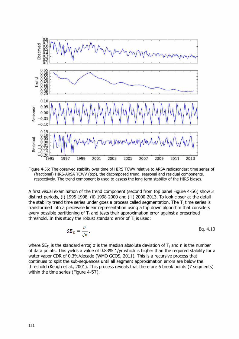
121

Figure 4-56: The observed stability over time of HIRS TCWV relative to ARSA radiosondes: time series of (fractional) HIRS-ARSA TCWV (top), the decomposed trend, seasonal and residual components, respectively. The trend component is used to assess the long term stability of the HIRS biases.

A first visual examination of the trend component (second from top panel Figure 4-56) show 3 distinct periods, (i) 1995-1998, (ii) 1998-2000 and (iii) 2000-2013. To look closer at the detail the stability trend time series under goes a process called segmentation. The Tt time series is transformed into a piecewise linear representation using a top down algorithm that considers every possible partitioning of Tt and tests their approximation error against a prescribed threshold. In this study the robust standard error of Tt is used:

Eq. 4.10

where SETt is the standard error, σ is the median absolute deviation of Tt and n is the number of data points. This yields a value of 0.83% 1/yr which is higher than the required stability for a water vapor CDR of 0.3%/decade (WMO GCOS, 2011). This is a recursive process that continues to split the sub-sequences until all segment approximation errors are below the threshold (Keogh et al., 2001). This process reveals that there are 6 break points (7 segments) within the time series (Figure 4-57).

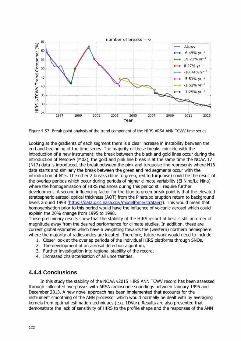
122

Figure 4-57: Break point analysis of the trend component of the HIRS-ARSA ANN TCWV time series.

Looking at the gradients of each segment there is a clear increase in instability between the end and beginning of the time series. The majority of these breaks coincide with the introduction of a new instrument; the break between the black and gold lines occur during the introduction of Metop-A (M02), the gold and pink line break is at the same time the NOAA 17 (N17) data is introduced, the break between the pink and turquoise line represents where N16 data starts and similarly the break between the green and red segments occur with the introduction of N15. The other 2 breaks (blue to green, red to turquoise) could be the result of the overlap periods which occur during periods of higher climate variability (El Nino/La Nina) where the homogenisation of HIRS radiances during this period still require further development. A second influencing factor for the blue to green break point is that the elevated stratospheric aerosol optical thickness (AOT) from the Pinatubo eruption return to background levels around 1998 (https://data.giss.nasa.gov/modelforce/strataer/). This would mean that homogenisation prior to this period would have the influence of volcanic aerosol which could explain the 20% change from 1995 to 1998. These preliminary results show that the stability of the HIRS record at best is still an order of magnitude away from the desired performance for climate studies. In addition, these are current global estimates which have a weighting towards the (western) northern hemisphere where the majority of radiosondes are located. Therefore, future work would need to include:

1. Closer look at the overlap periods of the individual HIRS platforms through SNOs, 2. The development of an aerosol detection algorithm, 3. Further investigation into regional stability of the record, 4. Increased characterisation of all uncertainties.

4.4.4 Conclusions

In this study the stability of the NOAA v2015 HIRS ANN TCWV record has been assessed through collocated overpasses with ARSA radiosonde soundings between January 1995 and December 2013. A new novel approach has been implemented that accounts for the instrument smoothing of the ANN processor which would normally be dealt with by averaging kernels from optimal estimation techniques (e.g. 1DVar). Results are also presented that demonstrate the lack of sensitivity of HIRS to the profile shape and the responses of the ANN

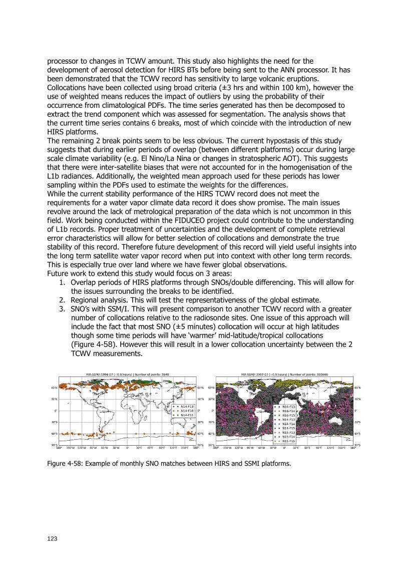
123

processor to changes in TCWV amount. This study also highlights the need for the development of aerosol detection for HIRS BTs before being sent to the ANN processor. It has been demonstrated that the TCWV record has sensitivity to large volcanic eruptions. Collocations have been collected using broad criteria (±3 hrs and within 100 km), however the use of weighted means reduces the impact of outliers by using the probability of their occurrence from climatological PDFs. The time series generated has then be decomposed to extract the trend component which was assessed for segmentation. The analysis shows that the current time series contains 6 breaks, most of which coincide with the introduction of new HIRS platforms. The remaining 2 break points seem to be less obvious. The current hypostasis of this study suggests that during earlier periods of overlap (between different platforms) occur during large scale climate variability (e.g. El Nino/La Nina or changes in stratospheric AOT). This suggests that there were inter-satellite biases that were not accounted for in the homogenisation of the L1b radiances. Additionally, the weighted mean approach used for these periods has lower sampling within the PDFs used to estimate the weights for the differences. While the current stability performance of the HIRS TCWV record does not meet the requirements for a water vapor climate data record it does show promise. The main issues revolve around the lack of metrological preparation of the data which is not uncommon in this field. Work being conducted within the FIDUCEO project could contribute to the understanding of L1b records. Proper treatment of uncertainties and the development of complete retrieval error characteristics will allow for better selection of collocations and demonstrate the true stability of this record. Therefore future development of this record will yield useful insights into the long term satellite water vapor record when put into context with other long term records. This is especially true over land where we have fewer global observations. Future work to extend this study would focus on 3 areas:

1. Overlap periods of HIRS platforms through SNOs/double differencing. This will allow for the issues surrounding the breaks to be identified.

2. Regional analysis. This will test the representativeness of the global estimate. 3. SNO’s with SSM/I. This will present comparison to another TCWV record with a greater

number of collocations relative to the radiosonde sites. One issue of this approach will include the fact that most SNO (±5 minutes) collocation will occur at high latitudes though some time periods will have ‘warmer’ mid-latitude/tropical collocations (Figure 4-58). However this will result in a lower collocation uncertainty between the 2 TCWV measurements.

Figure 4-58: Example of monthly SNO matches between HIRS and SSMI platforms.

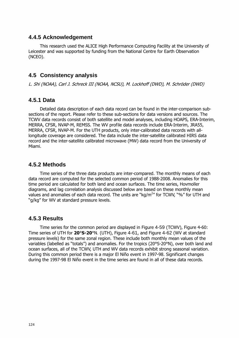
124

4.4.5 Acknowledgement

This research used the ALICE High Performance Computing Facility at the University of Leicester and was supported by funding from the National Centre for Earth Observation (NCEO).

4.5 Consistency analysis

L. Shi (NOAA), Carl J. Schreck III (NOAA, NCSU), M. Lockhoff (DWD), M. Schröder (DWD)

4.5.1 Data

Detailed data description of each data record can be found in the inter-comparison sub-sections of the report. Please refer to these sub-sections for data versions and sources. The TCWV data records consist of both satellite and model analyses, including HOAPS, ERA-Interim, MERRA, CFSR, NVAP-M, REMSS. The WV profile data records include ERA-Interim, JRA55, MERRA, CFSR, NVAP-M. For the UTH products, only inter-calibrated data records with all-longitude coverage are considered. The data include the inter-satellite calibrated HIRS data record and the inter-satellite calibrated microwave (MW) data record from the University of Miami.

4.5.2 Methods

Time series of the three data products are inter-compared. The monthly means of each data record are computed for the selected common period of 1988-2008. Anomalies for this time period are calculated for both land and ocean surfaces. The time series, Hovmoller diagrams, and lag correlation analysis discussed below are based on these monthly mean values and anomalies of each data record. The units are “kg/m2” for TCWV, “%” for UTH and “g/kg” for WV at standard pressure levels.

4.5.3 Results

Time series for the common period are displayed in Figure 4-59 (TCWV), Figure 4-60: Time series of UTH for 20°S-20°N. (UTH), Figure 4-61, and Figure 4-62 (WV at standard pressure levels) for the same zonal region. These include both monthly mean values of the variables (labelled as “totals”) and anomalies. For the tropics (20°S-20°N), over both land and ocean surfaces, all of the TCWV, UTH and WV data records exhibit strong seasonal variation. During this common period there is a major El Niño event in 1997-98. Significant changes during the 1997-98 El Niño event in the time series are found in all of these data records.

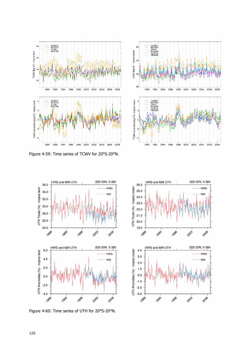
125

Figure 4-59: Time series of TCWV for 20°S-20°N.

Figure 4-60: Time series of UTH for 20°S-20°N.

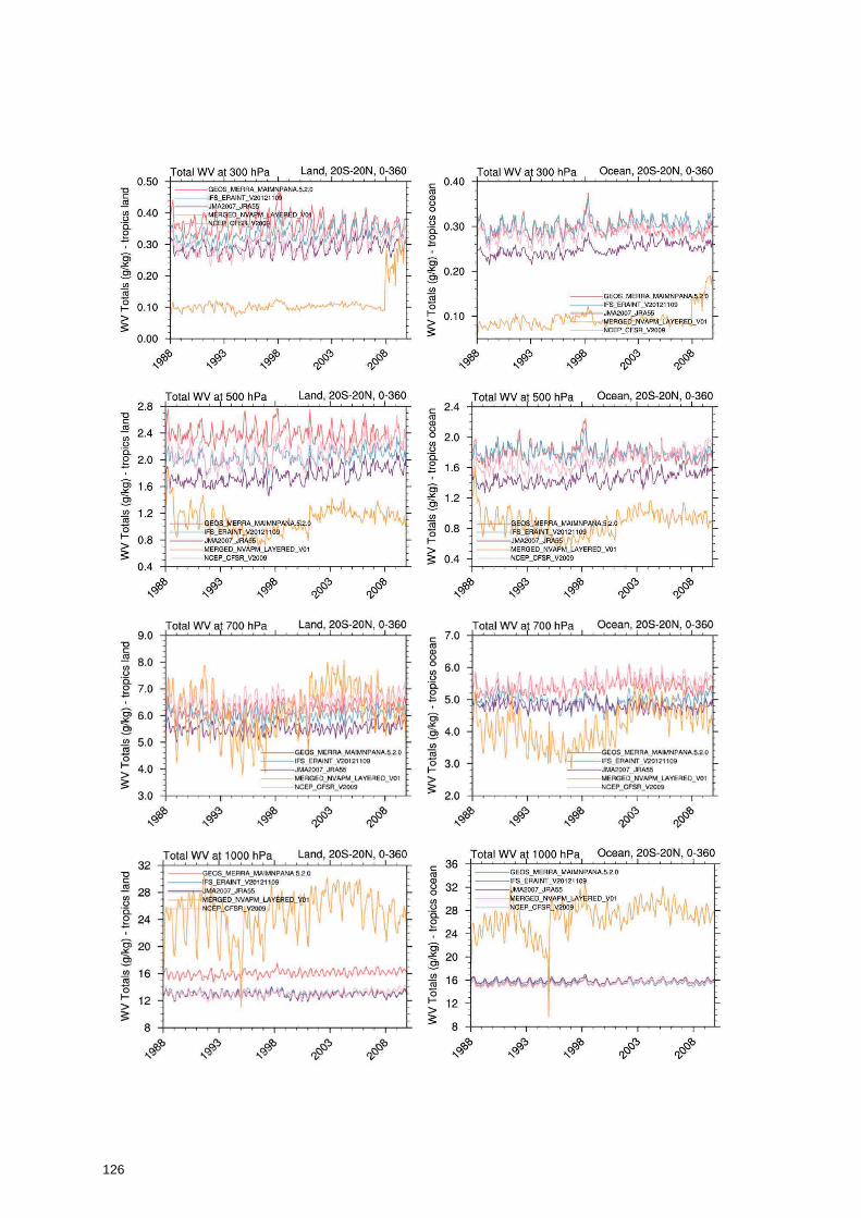
126

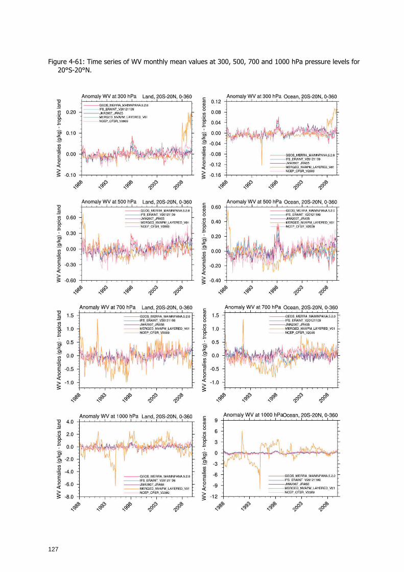
127

Figure 4-61: Time series of WV monthly mean values at 300, 500, 700 and 1000 hPa pressure levels for 20°S-20°N.

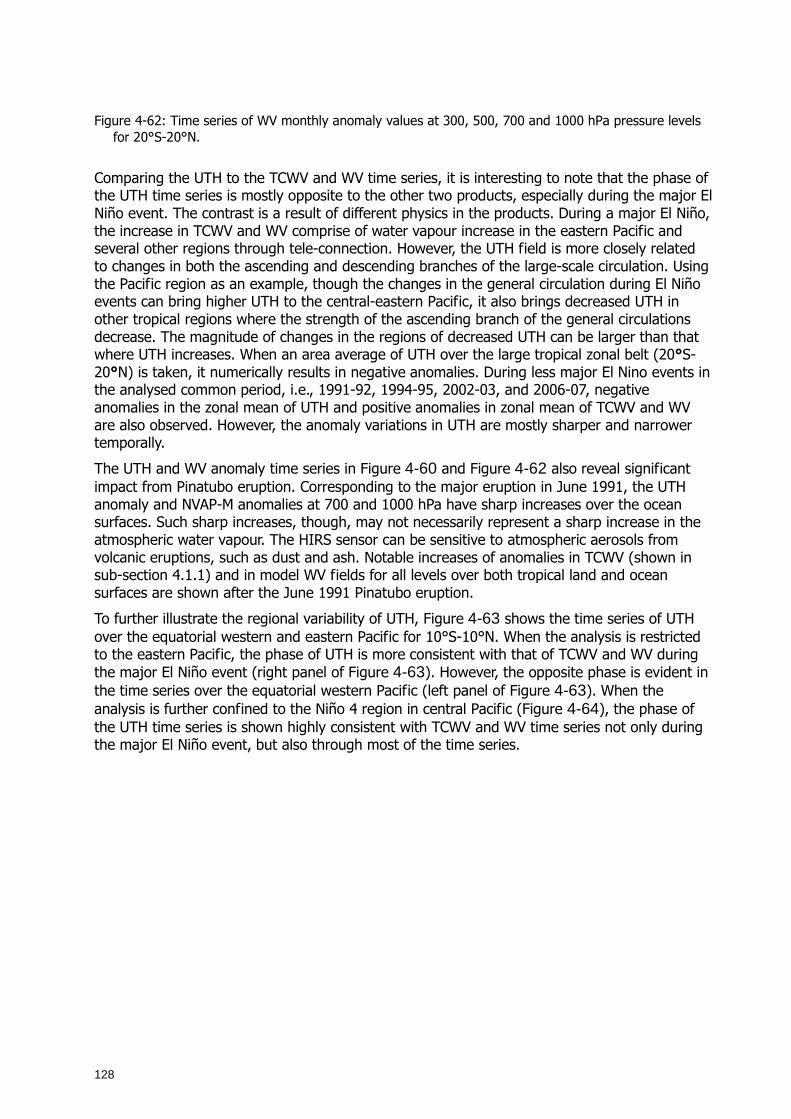
128

Figure 4-62: Time series of WV monthly anomaly values at 300, 500, 700 and 1000 hPa pressure levels for 20°S-20°N.

Comparing the UTH to the TCWV and WV time series, it is interesting to note that the phase of the UTH time series is mostly opposite to the other two products, especially during the major El Niño event. The contrast is a result of different physics in the products. During a major El Niño, the increase in TCWV and WV comprise of water vapour increase in the eastern Pacific and several other regions through tele-connection. However, the UTH field is more closely related to changes in both the ascending and descending branches of the large-scale circulation. Using the Pacific region as an example, though the changes in the general circulation during El Niño events can bring higher UTH to the central-eastern Pacific, it also brings decreased UTH in other tropical regions where the strength of the ascending branch of the general circulations decrease. The magnitude of changes in the regions of decreased UTH can be larger than that where UTH increases. When an area average of UTH over the large tropical zonal belt (20°S-20°N) is taken, it numerically results in negative anomalies. During less major El Nino events in the analysed common period, i.e., 1991-92, 1994-95, 2002-03, and 2006-07, negative anomalies in the zonal mean of UTH and positive anomalies in zonal mean of TCWV and WV are also observed. However, the anomaly variations in UTH are mostly sharper and narrower temporally.

The UTH and WV anomaly time series in Figure 4-60 and Figure 4-62 also reveal significant impact from Pinatubo eruption. Corresponding to the major eruption in June 1991, the UTH anomaly and NVAP-M anomalies at 700 and 1000 hPa have sharp increases over the ocean surfaces. Such sharp increases, though, may not necessarily represent a sharp increase in the atmospheric water vapour. The HIRS sensor can be sensitive to atmospheric aerosols from volcanic eruptions, such as dust and ash. Notable increases of anomalies in TCWV (shown in sub-section 4.1.1) and in model WV fields for all levels over both tropical land and ocean surfaces are shown after the June 1991 Pinatubo eruption.

To further illustrate the regional variability of UTH, Figure 4-63 shows the time series of UTH over the equatorial western and eastern Pacific for 10°S-10°N. When the analysis is restricted to the eastern Pacific, the phase of UTH is more consistent with that of TCWV and WV during the major El Niño event (right panel of Figure 4-63). However, the opposite phase is evident in the time series over the equatorial western Pacific (left panel of Figure 4-63). When the analysis is further confined to the Niño 4 region in central Pacific (Figure 4-64), the phase of the UTH time series is shown highly consistent with TCWV and WV time series not only during the major El Niño event, but also through most of the time series.

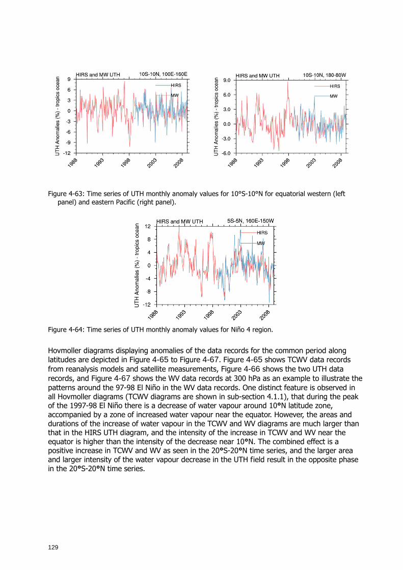
129

Figure 4-63: Time series of UTH monthly anomaly values for 10°S-10°N for equatorial western (left

panel) and eastern Pacific (right panel).

Figure 4-64: Time series of UTH monthly anomaly values for Niño 4 region.

Hovmoller diagrams displaying anomalies of the data records for the common period along latitudes are depicted in Figure 4-65 to Figure 4-67. Figure 4-65 shows TCWV data records from reanalysis models and satellite measurements, Figure 4-66 shows the two UTH data records, and Figure 4-67 shows the WV data records at 300 hPa as an example to illustrate the patterns around the 97-98 El Niño in the WV data records. One distinct feature is observed in all Hovmoller diagrams (TCWV diagrams are shown in sub-section 4.1.1), that during the peak of the 1997-98 El Niño there is a decrease of water vapour around 10°N latitude zone, accompanied by a zone of increased water vapour near the equator. However, the areas and durations of the increase of water vapour in the TCWV and WV diagrams are much larger than that in the HIRS UTH diagram, and the intensity of the increase in TCWV and WV near the equator is higher than the intensity of the decrease near 10°N. The combined effect is a positive increase in TCWV and WV as seen in the 20°S-20°N time series, and the larger area and larger intensity of the water vapour decrease in the UTH field result in the opposite phase in the 20°S-20°N time series.

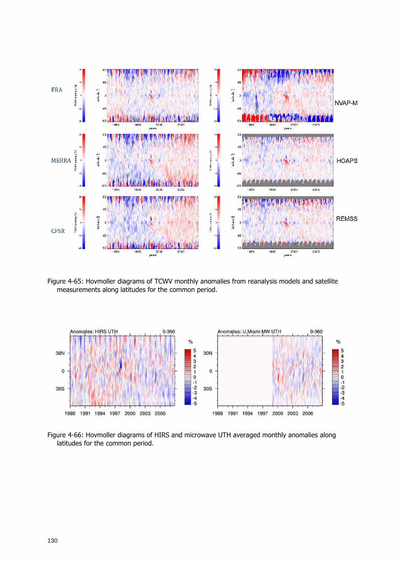
130

Figure 4-65: Hovmoller diagrams of TCWV monthly anomalies from reanalysis models and satellite

measurements along latitudes for the common period.

Figure 4-66: Hovmoller diagrams of HIRS and microwave UTH averaged monthly anomalies along

latitudes for the common period.

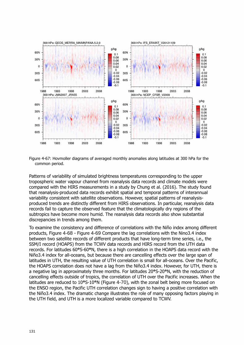
131

Figure 4-67: Hovmoller diagrams of averaged monthly anomalies along latitudes at 300 hPa for the

common period.

Patterns of variability of simulated brightness temperatures corresponding to the upper tropospheric water vapour channel from reanalysis data records and climate models were compared with the HIRS measurements in a study by Chung et al. (2016). The study found that reanalysis-produced data records exhibit spatial and temporal patterns of interannual variability consistent with satellite observations. However, spatial patterns of reanalysis-produced trends are distinctly different from HIRS observations. In particular, reanalysis data records fail to capture the observed feature that the climatologically dry regions of the subtropics have become more humid. The reanalysis data records also show substantial discrepancies in trends among them.

To examine the consistency and difference of correlations with the Niño index among different products, Figure 4-68 - Figure 4-69 Compare the lag correlations with the Nino3.4 index between two satellite records of different products that have long-term time series, i.e., the SSM/I record (HOAPS) from the TCWV data records and HIRS record from the UTH data records. For latitudes 60°S-60°N, there is a high correlation in the HOAPS data record with the Niño3.4 index for all-oceans, but because there are cancelling effects over the large span of latitudes in UTH, the resulting value of UTH correlation is small for all-oceans. Over the Pacific, the HOAPS correlation does not have a lag from the Niño3.4 index. However, for UTH, there is a negative lag in approximately three months. For latitudes 20°S-20°N, with the reduction of cancelling effects outside of tropics, the correlation of UTH over the Pacific increases. When the latitudes are reduced to 10°S-10°N (Figure 4-70), with the zonal belt being more focused on the ENSO region, the Pacific UTH correlation changes sign to having a positive correlation with the Niño3.4 index. The dramatic change illustrates the role of many opposing factors playing in the UTH field, and UTH is a more localized variable compared to TCWV.

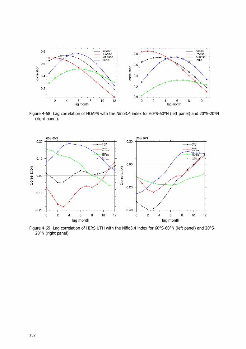
132

Figure 4-68: Lag correlation of HOAPS with the Niño3.4 index for 60°S-60°N (left panel) and 20°S-20°N

(right panel).

Figure 4-69: Lag correlation of HIRS UTH with the Niño3.4 index for 60°S-60°N (left panel) and 20°S-

20°N (right panel).

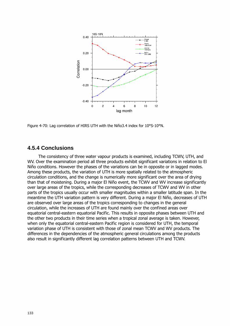
133

Figure 4-70: Lag correlation of HIRS UTH with the Niño3.4 index for 10°S-10°N.

4.5.4 Conclusions

The consistency of three water vapour products is examined, including TCWV, UTH, and WV. Over the examination period all three products exhibit significant variations in relation to El Niño conditions. However the phases of the variations can be in opposite or in lagged modes. Among these products, the variation of UTH is more spatially related to the atmospheric circulation conditions, and the change is numerically more significant over the area of drying than that of moistening. During a major El Niño event, the TCWV and WV increase significantly over large areas of the tropics, while the corresponding decreases of TCWV and WV in other parts of the tropics usually occur with smaller magnitudes within a smaller latitude span. In the meantime the UTH variation pattern is very different. During a major El Niño, decreases of UTH are observed over large areas of the tropics corresponding to changes in the general circulation, while the increases of UTH are found mainly over the confined areas over equatorial central-eastern equatorial Pacific. This results in opposite phases between UTH and the other two products in their time series when a tropical zonal average is taken. However, when only the equatorial central-eastern Pacific region is considered for UTH, the temporal variation phase of UTH is consistent with those of zonal mean TCWV and WV products. The differences in the dependencies of the atmospheric general circulations among the products also result in significantly different lag correlation patterns between UTH and TCWV.

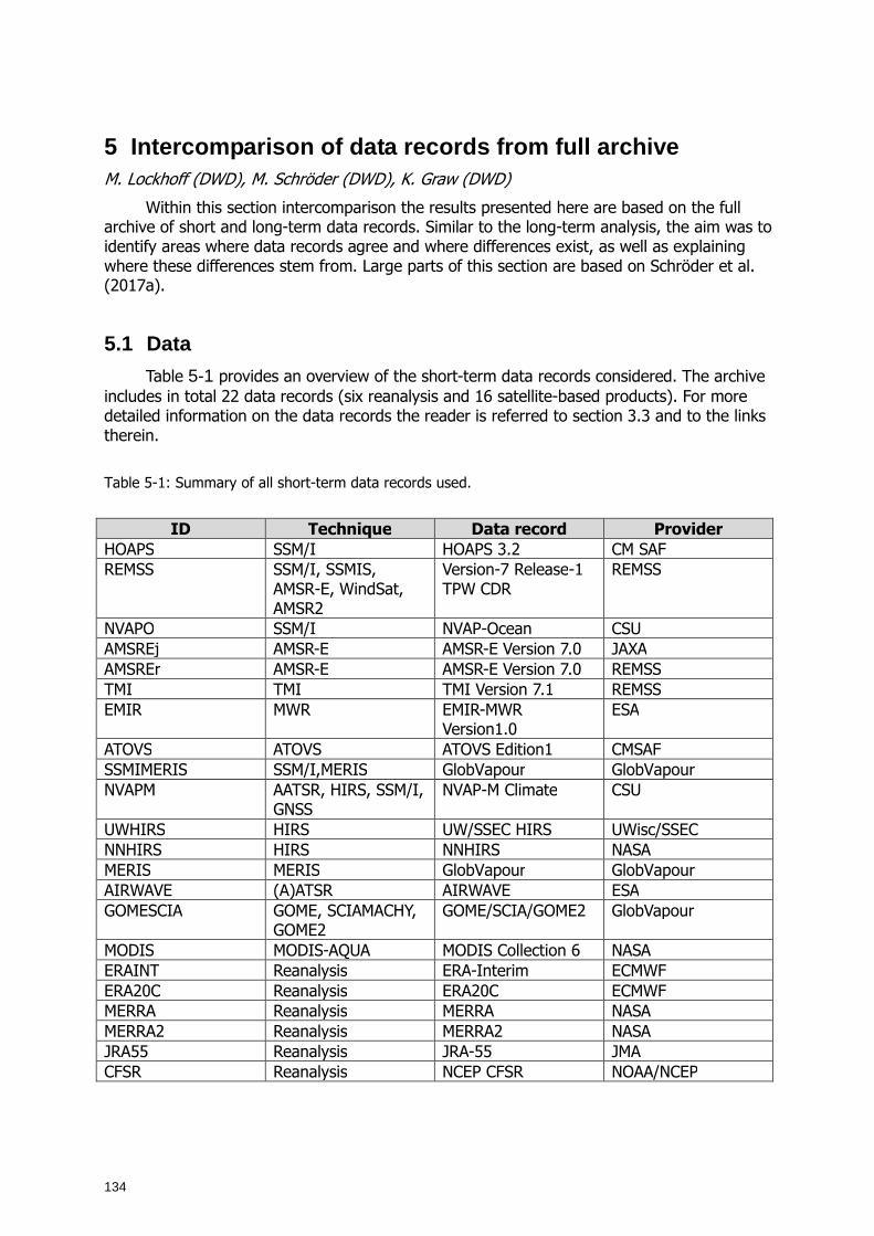
134

5 Intercomparison of data records from full archive M. Lockhoff (DWD), M. Schröder (DWD), K. Graw (DWD)

Within this section intercomparison the results presented here are based on the full archive of short and long-term data records. Similar to the long-term analysis, the aim was to identify areas where data records agree and where differences exist, as well as explaining where these differences stem from. Large parts of this section are based on Schröder et al. (2017a).

5.1 Data

Table 5-1 provides an overview of the short-term data records considered. The archive includes in total 22 data records (six reanalysis and 16 satellite-based products). For more detailed information on the data records the reader is referred to section 3.3 and to the links therein.

Table 5-1: Summary of all short-term data records used.

ID Technique Data record Provider

HOAPS SSM/I HOAPS 3.2 CM SAF REMSS SSM/I, SSMIS,

AMSR-E, WindSat, AMSR2

Version-7 Release-1 TPW CDR

REMSS

NVAPO SSM/I NVAP-Ocean CSU AMSREj AMSR-E AMSR-E Version 7.0 JAXA AMSREr AMSR-E AMSR-E Version 7.0 REMSS TMI TMI TMI Version 7.1 REMSS EMIR MWR EMIR-MWR

Version1.0 ESA

ATOVS ATOVS ATOVS Edition1 CMSAF SSMIMERIS SSM/I,MERIS GlobVapour GlobVapour NVAPM AATSR, HIRS, SSM/I,

GNSS NVAP-M Climate CSU

UWHIRS HIRS UW/SSEC HIRS UWisc/SSEC NNHIRS HIRS NNHIRS NASA MERIS MERIS GlobVapour GlobVapour AIRWAVE (A)ATSR AIRWAVE ESA GOMESCIA GOME, SCIAMACHY,

GOME2 GOME/SCIA/GOME2 GlobVapour

MODIS MODIS-AQUA MODIS Collection 6 NASA ERAINT Reanalysis ERA-Interim ECMWF ERA20C Reanalysis ERA20C ECMWF MERRA Reanalysis MERRA NASA MERRA2 Reanalysis MERRA2 NASA JRA55 Reanalysis JRA-55 JMA CFSR Reanalysis NCEP CFSR NOAA/NCEP

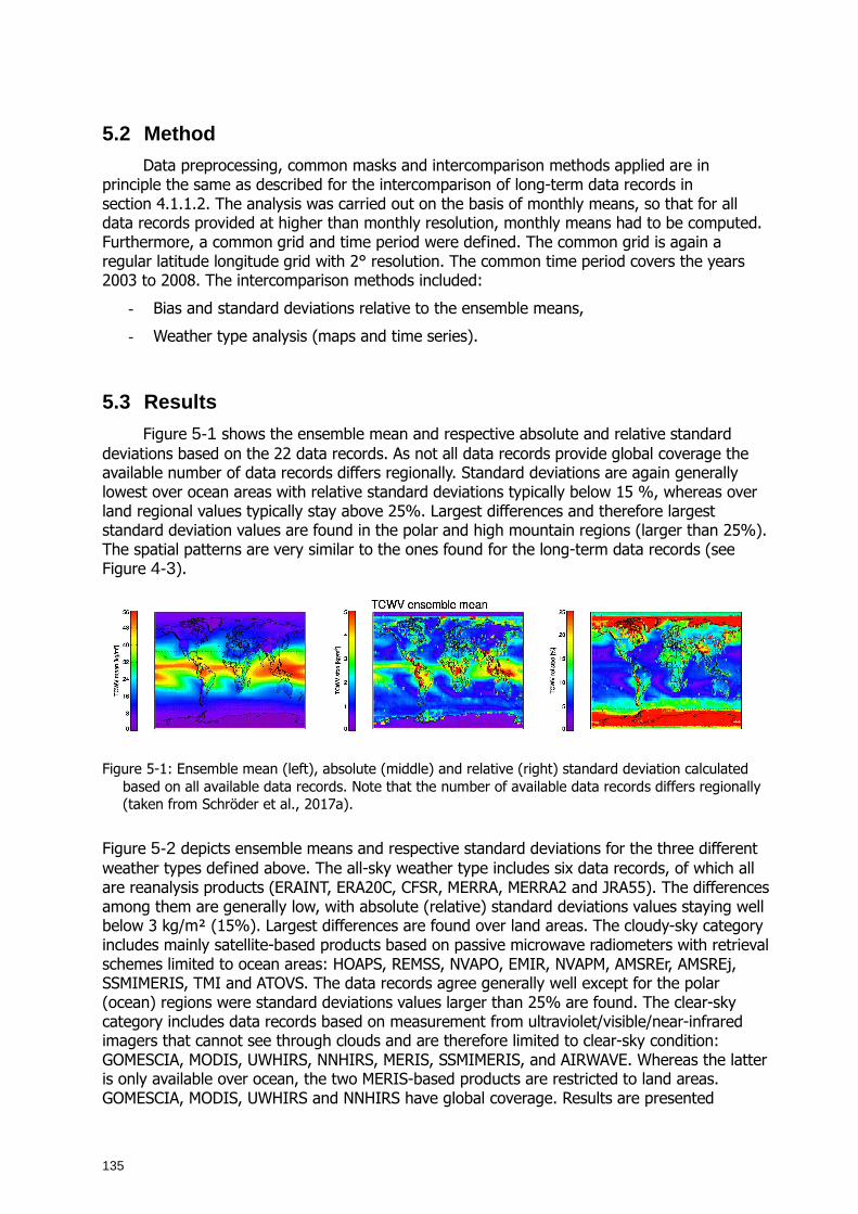
135

5.2 Method

Data preprocessing, common masks and intercomparison methods applied are in principle the same as described for the intercomparison of long-term data records in section 4.1.1.2. The analysis was carried out on the basis of monthly means, so that for all data records provided at higher than monthly resolution, monthly means had to be computed. Furthermore, a common grid and time period were defined. The common grid is again a regular latitude longitude grid with 2° resolution. The common time period covers the years 2003 to 2008. The intercomparison methods included:

- Bias and standard deviations relative to the ensemble means,

- Weather type analysis (maps and time series).

5.3 Results

Figure 5-1 shows the ensemble mean and respective absolute and relative standard deviations based on the 22 data records. As not all data records provide global coverage the available number of data records differs regionally. Standard deviations are again generally lowest over ocean areas with relative standard deviations typically below 15 %, whereas over land regional values typically stay above 25%. Largest differences and therefore largest standard deviation values are found in the polar and high mountain regions (larger than 25%). The spatial patterns are very similar to the ones found for the long-term data records (see Figure 4-3).

Figure 5-1: Ensemble mean (left), absolute (middle) and relative (right) standard deviation calculated

based on all available data records. Note that the number of available data records differs regionally (taken from Schröder et al., 2017a).

Figure 5-2 depicts ensemble means and respective standard deviations for the three different weather types defined above. The all-sky weather type includes six data records, of which all are reanalysis products (ERAINT, ERA20C, CFSR, MERRA, MERRA2 and JRA55). The differences among them are generally low, with absolute (relative) standard deviations values staying well below 3 kg/m² (15%). Largest differences are found over land areas. The cloudy-sky category includes mainly satellite-based products based on passive microwave radiometers with retrieval schemes limited to ocean areas: HOAPS, REMSS, NVAPO, EMIR, NVAPM, AMSREr, AMSREj, SSMIMERIS, TMI and ATOVS. The data records agree generally well except for the polar (ocean) regions were standard deviations values larger than 25% are found. The clear-sky category includes data records based on measurement from ultraviolet/visible/near-infrared imagers that cannot see through clouds and are therefore limited to clear-sky condition: GOMESCIA, MODIS, UWHIRS, NNHIRS, MERIS, SSMIMERIS, and AIRWAVE. Whereas the latter is only available over ocean, the two MERIS-based products are restricted to land areas. GOMESCIA, MODIS, UWHIRS and NNHIRS have global coverage. Results are presented

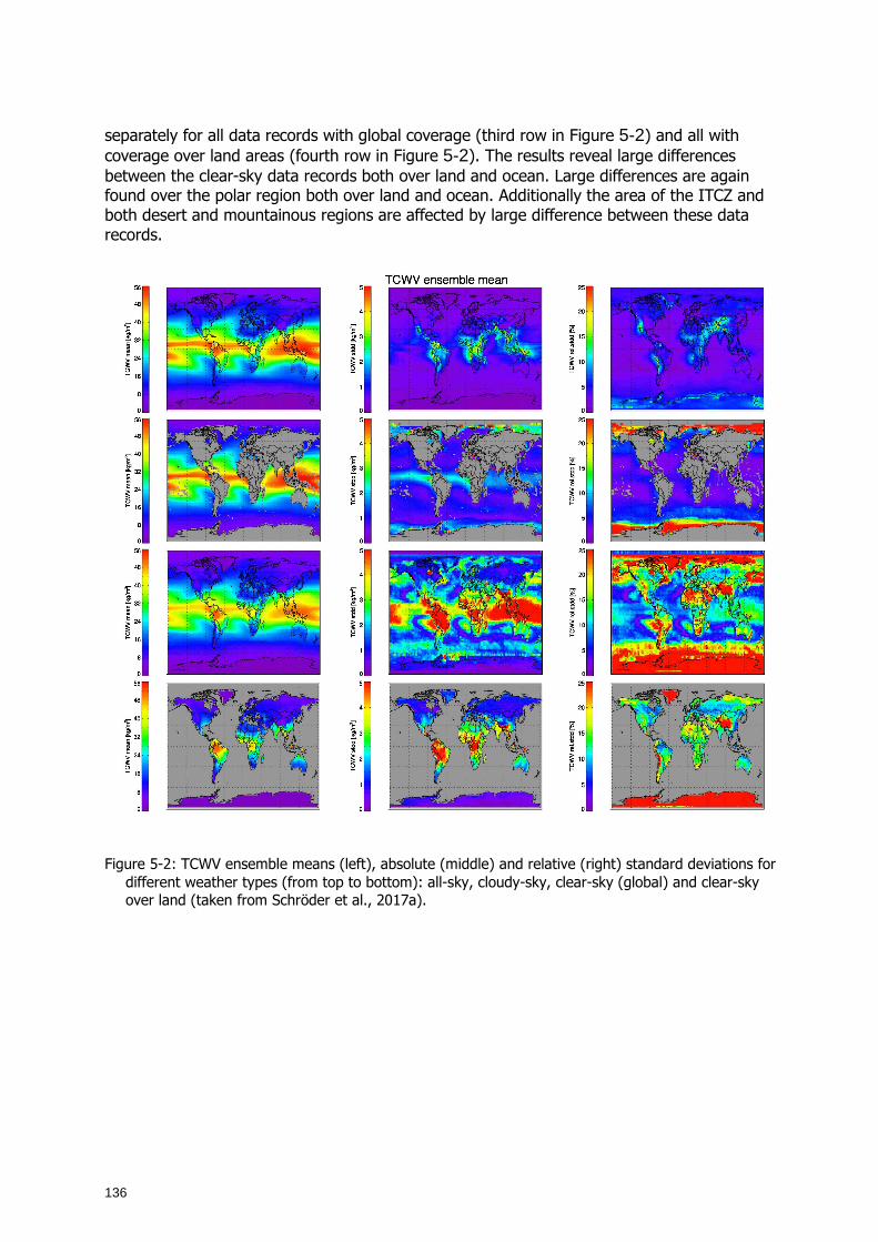
136

separately for all data records with global coverage (third row in Figure 5-2) and all with coverage over land areas (fourth row in Figure 5-2). The results reveal large differences between the clear-sky data records both over land and ocean. Large differences are again found over the polar region both over land and ocean. Additionally the area of the ITCZ and both desert and mountainous regions are affected by large difference between these data records.

Figure 5-2: TCWV ensemble means (left), absolute (middle) and relative (right) standard deviations for different weather types (from top to bottom): all-sky, cloudy-sky, clear-sky (global) and clear-sky over land (taken from Schröder et al., 2017a).

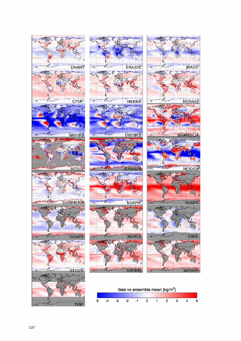
137

138

Figure 5-3: TCWV bias relative to the ensemble mean for all 22 ensemble members (adapted from Schröder et al., 2017a).

In order to investigate in more detail which data records cause the different areas with increased standard deviation values the bias relative to the ensemble mean was calculated for each of the 22 data records. The corresponding maps are shown in Figure 5-3. All IR-based retrievals (NNHIRS, UWHIRS, AIRWAVE, MODIS) exhibit large positive biases over subtropical high pressure zones. GOMESCIA also exhibits a bias feature in this area but shows negative bias, thus lower values than the other IR-based retrievals. Over land IR-based behaviour differs, NNHIRS reports much less TCWV than the ensemble mean whereas both MODIS and NVAP-M show a large positive bias, especially over the tropical Africa. That’s also where the reanalysis data records differ (as already seen in the intercomparison of the long-term data records). ERA20C and JRA55 show lower values compared to the other reanalyses. Over the ocean areas biases are generally low for all microwave based and reanaylsis products except JRA-55, ERA20C, NVAP-O and NVAP-M which show relatively large negative (reanalyses) and positive (NVAP-M, NVAP-O) biases in the tropics. Figure 5-4 shows time series of TCWV and TCWV anomalies for the tropical ocean with the data records grouped according to the different weather types. They served to investigate the consistency of the temporal variability and check for inhomogeneities in the data records as possible source for differences found between the data records and to assess the presence of systematic differences among the weather types. The reanalysis (all-sky) data show good agreement over time over the tropical ocean area with a spread of around 2 kg/m² among the different data records. This is not too surprising as the spatial maps already showed the good agreement among the reanalyses over ocean. For the two other weather types, however, we found areas of larger differences. Accordingly, a large spread among the data records in the order of 5 kg/m² and 6 kg/m² for the cloudy-sky and clear-sky weather types was found, respectively. Concerning the cloud-sky data records the spread is mainly due to NVAP-O and NVAP-M which both show larger values than the others which actually agree within 2 kg/m². Despite the offset between the data records the anomalies agree well between the cloud-sky data records. Only the EMIR anomalies exhibits individual months with larger differences (round 1 kg/m²) in 2005 and 2006 with respect to the other anomaly time series. For the clear-sky data records an offset between the individual records and differences with respect to the seasonal cycle (maxima shifted) and its magnitude were found. GOMESCIA and MODIS show the largest seasonal cycle. Best agreement is found between GOMESCIA, AIRWAVE and UWHIRS (within 2 kg/m²) from 2007 onwards, which is due to a decrease in TCWV for GOMESCIA and an increase in TCWV for UWHIRS happening round that time. This change coincides with the launch of MetOp-A end of 2006 with both GOME-2 and an HIRS instrument onboard.

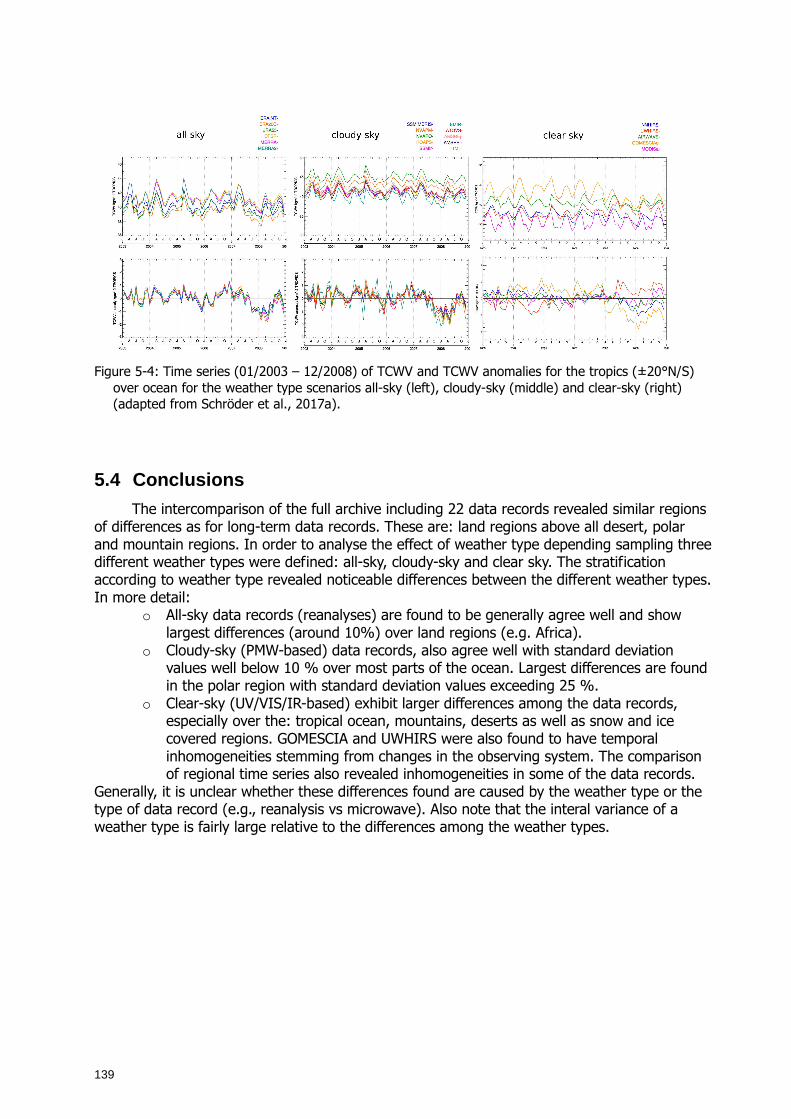
139

Figure 5-4: Time series (01/2003 – 12/2008) of TCWV and TCWV anomalies for the tropics (±20°N/S)

over ocean for the weather type scenarios all-sky (left), cloudy-sky (middle) and clear-sky (right) (adapted from Schröder et al., 2017a).

5.4 Conclusions

The intercomparison of the full archive including 22 data records revealed similar regions of differences as for long-term data records. These are: land regions above all desert, polar and mountain regions. In order to analyse the effect of weather type depending sampling three different weather types were defined: all-sky, cloudy-sky and clear sky. The stratification according to weather type revealed noticeable differences between the different weather types. In more detail:

o All-sky data records (reanalyses) are found to be generally agree well and show largest differences (around 10%) over land regions (e.g. Africa).

o Cloudy-sky (PMW-based) data records, also agree well with standard deviation values well below 10 % over most parts of the ocean. Largest differences are found in the polar region with standard deviation values exceeding 25 %.

o Clear-sky (UV/VIS/IR-based) exhibit larger differences among the data records, especially over the: tropical ocean, mountains, deserts as well as snow and ice covered regions. GOMESCIA and UWHIRS were also found to have temporal inhomogeneities stemming from changes in the observing system. The comparison of regional time series also revealed inhomogeneities in some of the data records.

Generally, it is unclear whether these differences found are caused by the weather type or the type of data record (e.g., reanalysis vs microwave). Also note that the interal variance of a weather type is fairly large relative to the differences among the weather types.

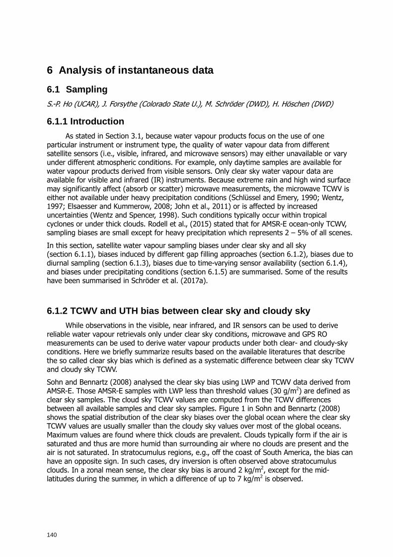
140

6 Analysis of instantaneous data

6.1 Sampling

S.-P. Ho (UCAR), J. Forsythe (Colorado State U.), M. Schröder (DWD), H. Höschen (DWD)

6.1.1 Introduction

As stated in Section 3.1, because water vapour products focus on the use of one particular instrument or instrument type, the quality of water vapour data from different satellite sensors (i.e., visible, infrared, and microwave sensors) may either unavailable or vary under different atmospheric conditions. For example, only daytime samples are available for water vapour products derived from visible sensors. Only clear sky water vapour data are available for visible and infrared (IR) instruments. Because extreme rain and high wind surface may significantly affect (absorb or scatter) microwave measurements, the microwave TCWV is either not available under heavy precipitation conditions (Schlüssel and Emery, 1990; Wentz, 1997; Elsaesser and Kummerow, 2008; John et al., 2011) or is affected by increased uncertainties (Wentz and Spencer, 1998). Such conditions typically occur within tropical cyclones or under thick clouds. Rodell et al., (2015) stated that for AMSR-E ocean-only TCWV, sampling biases are small except for heavy precipitation which represents 2 – 5% of all scenes.

In this section, satellite water vapour sampling biases under clear sky and all sky (section 6.1.1), biases induced by different gap filling approaches (section 6.1.2), biases due to diurnal sampling (section 6.1.3), biases due to time-varying sensor availability (section 6.1.4), and biases under precipitating conditions (section 6.1.5) are summarised. Some of the results have been summarised in Schröder et al. (2017a).

6.1.2 TCWV and UTH bias between clear sky and cloud y sky

While observations in the visible, near infrared, and IR sensors can be used to derive reliable water vapour retrievals only under clear sky conditions, microwave and GPS RO measurements can be used to derive water vapour products under both clear- and cloudy-sky conditions. Here we briefly summarize results based on the available literatures that describe the so called clear sky bias which is defined as a systematic difference between clear sky TCWV and cloudy sky TCWV.

Sohn and Bennartz (2008) analysed the clear sky bias using LWP and TCWV data derived from AMSR-E. Those AMSR-E samples with LWP less than threshold values (30 g/m2) are defined as clear sky samples. The cloud sky TCWV values are computed from the TCWV differences between all available samples and clear sky samples. Figure 1 in Sohn and Bennartz (2008) shows the spatial distribution of the clear sky biases over the global ocean where the clear sky TCWV values are usually smaller than the cloudy sky values over most of the global oceans. Maximum values are found where thick clouds are prevalent. Clouds typically form if the air is saturated and thus are more humid than surrounding air where no clouds are present and the air is not saturated. In stratocumulus regions, e.g., off the coast of South America, the bias can have an opposite sign. In such cases, dry inversion is often observed above stratocumulus clouds. In a zonal mean sense, the clear sky bias is around 2 kg/m2, except for the mid-latitudes during the summer, in which a difference of up to 7 kg/m2 is observed.

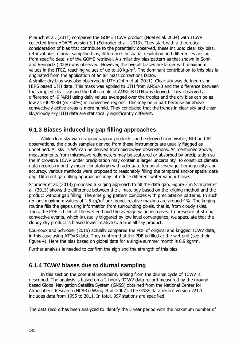
141

Mieruch et al. (2011) compared the GOME TCWV product (Noel et al. 2004) with TCWV collected from HOAPS version 3.1 (Schröder et al., 2013). They start with a theoretical consideration of bias that contribute to the potentially observed, these include: clear sky bias, retrieval bias, diurnal sampling bias, differences in spatial resolution and differences arising from specific details of the GOME retrieval. A similar dry bias pattern as that shown in Sohn and Bennartz (2008) was observed. However, the overall biases are larger with maximum values in the ITCZ, reaching values of up to 10 kg/m2. The dominant contribution to this bias is originated from the application of an air mass corrections factor. A similar dry bias was also observed in UTH (John et al. 2011). Clear sky was defined using HIRS based UTH data. This mask was applied to UTH from AMSU-B and the difference between the sampled clear sky and the full sample of AMSU-B UTH was derived. They observed a difference of -9 %RH using daily values averaged over the tropics and the dry bias can be as low as -30 %RH (or -50%) in convective regions. This may be in part because air above convectively active areas is more humid. They concluded that the trends in clear sky and clear sky/cloudy sky UTH data are statistically significantly different.

6.1.3 Biases induced by gap filling approaches

While clear sky water vapour vapour products can be derived from visible, NIR and IR observations, the cloudy samples derived from these instruments are usually flagged as undefined. All sky TCWV can be derived from microwave observations. As mentioned above, measurements from microwave radiometers may be scattered or absorbed by precipitation so the microwave TCWV under precipitation may contain a larger uncertainty. To construct climate data records (monthly mean climatology) with adequate temporal coverage, homogeneity, and accuracy, various methods were proposed to reasonably filling the temporal and/or spatial data gap. Different gap filling approaches may introduce different water vapour biases.

Schröder et al. (2013) proposed a kriging approach to fill the data gap. Figure 2 in Schröder et al. (2013) shows the difference between the climatology based on the kriging method and the product without gap filling. The emerging pattern coincides with precipitation patterns. In such regions maximum values of 1.5 kg/m2 are found, relative maxima are around 4%. The kriging routine fills the gaps using information from surrounding pixels, that is, from cloudy skies. Thus, the PDF is filled at the wet end and the average value increases. In presence of strong convective events, which is usually triggered by low level convergence, we speculate that the cloudy sky product is biased lower relative to a true all sky product.

Courcoux and Schröder (2015) actually compared the PDF of original and krigged TCWV data, in this case using ATOVS data. They confirm that the PDF is filled at the wet end (see their figure 4). Here the bias based on global data for a single summer month is 0.9 kg/m2.

Further analysis is needed to confirm the sign and the strength of this bias.

6.1.4 TCWV biases due to diurnal sampling

In this section the potential uncertainty arising from the diurnal cycle of TCWV is described. The analysis is based on a 2-hourly TCWV data record measured by the ground-based Global Navigation Satellite System (GNSS) obtained from the National Center for Atmospheric Research (NCAR) (Wang et al. 2007). The GNSS data record version 721.1 includes data from 1995 to 2011. In total, 997 stations are specified.

The data record has been analyzed to identify the 5 year period with the maximum number of

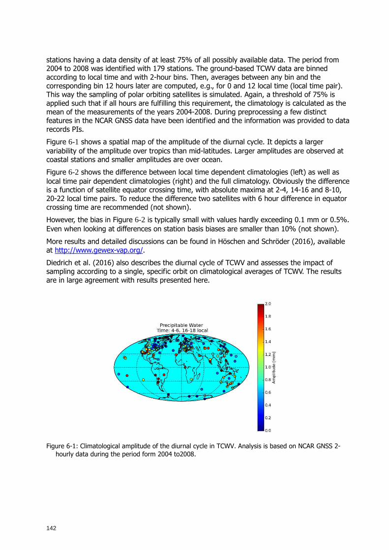
142

stations having a data density of at least 75% of all possibly available data. The period from 2004 to 2008 was identified with 179 stations. The ground-based TCWV data are binned according to local time and with 2-hour bins. Then, averages between any bin and the corresponding bin 12 hours later are computed, e.g., for 0 and 12 local time (local time pair). This way the sampling of polar orbiting satellites is simulated. Again, a threshold of 75% is applied such that if all hours are fulfilling this requirement, the climatology is calculated as the mean of the measurements of the years 2004-2008. During preprocessing a few distinct features in the NCAR GNSS data have been identified and the information was provided to data records PIs.

Figure 6-1 shows a spatial map of the amplitude of the diurnal cycle. It depicts a larger variability of the amplitude over tropics than mid-latitudes. Larger amplitudes are observed at coastal stations and smaller amplitudes are over ocean.

Figure 6-2 shows the difference between local time dependent climatologies (left) as well as local time pair dependent climatologies (right) and the full climatology. Obviously the difference is a function of satellite equator crossing time, with absolute maxima at 2-4, 14-16 and 8-10, 20-22 local time pairs. To reduce the difference two satellites with 6 hour difference in equator crossing time are recommended (not shown).

However, the bias in Figure 6-2 is typically small with values hardly exceeding 0.1 mm or 0.5%. Even when looking at differences on station basis biases are smaller than 10% (not shown).

More results and detailed discussions can be found in Höschen and Schröder (2016), available at http://www.gewex-vap.org/.

Diedrich et al. (2016) also describes the diurnal cycle of TCWV and assesses the impact of sampling according to a single, specific orbit on climatological averages of TCWV. The results are in large agreement with results presented here.

Figure 6-1: Climatological amplitude of the diurnal cycle in TCWV. Analysis is based on NCAR GNSS 2-

hourly data during the period form 2004 to2008.

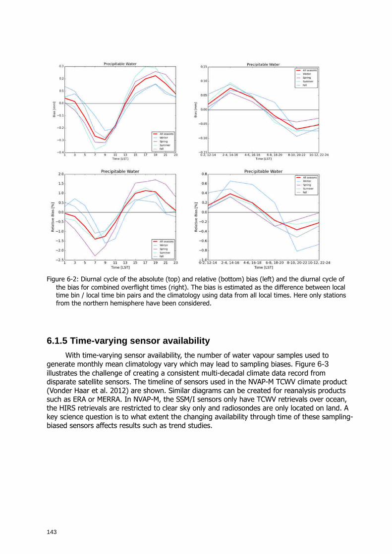
143

Figure 6-2: Diurnal cycle of the absolute (top) and relative (bottom) bias (left) and the diurnal cycle of

the bias for combined overflight times (right). The bias is estimated as the difference between local time bin / local time bin pairs and the climatology using data from all local times. Here only stations from the northern hemisphere have been considered.

6.1.5 Time-varying sensor availability

With time-varying sensor availability, the number of water vapour samples used to generate monthly mean climatology vary which may lead to sampling biases. Figure 6-3 illustrates the challenge of creating a consistent multi-decadal climate data record from disparate satellite sensors. The timeline of sensors used in the NVAP-M TCWV climate product (Vonder Haar et al. 2012) are shown. Similar diagrams can be created for reanalysis products such as ERA or MERRA. In NVAP-M, the SSM/I sensors only have TCWV retrievals over ocean, the HIRS retrievals are restricted to clear sky only and radiosondes are only located on land. A key science question is to what extent the changing availability through time of these sampling-biased sensors affects results such as trend studies.

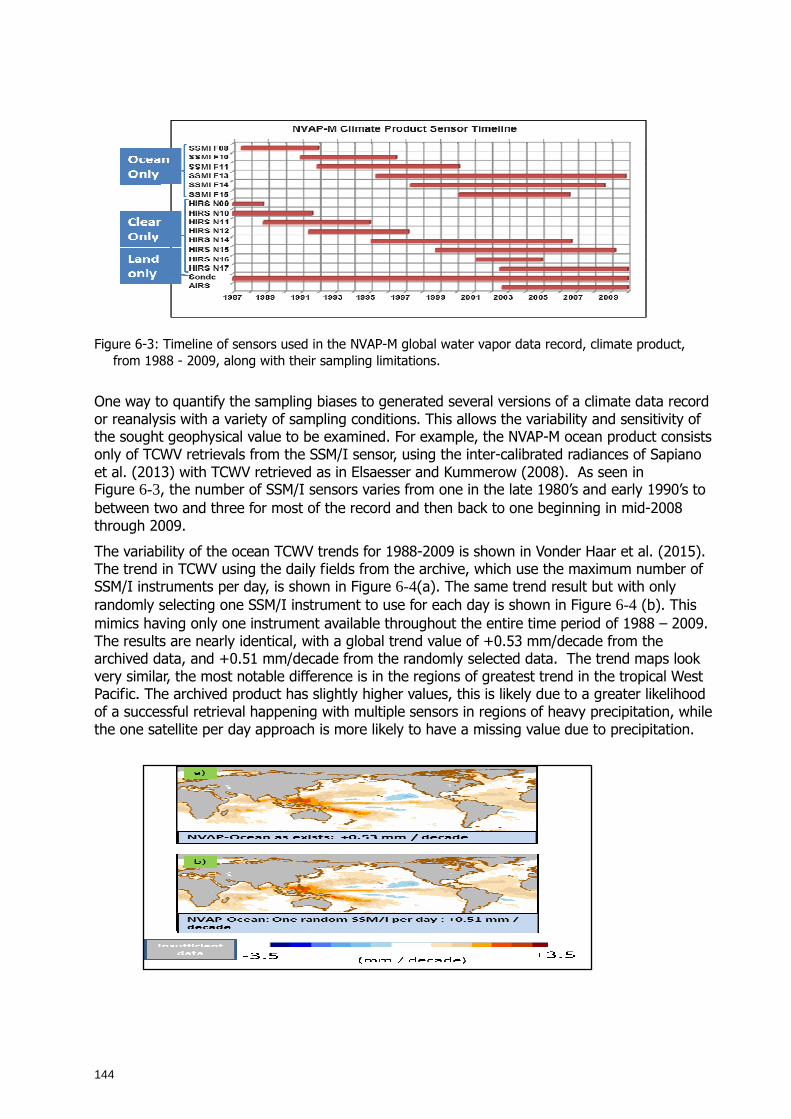
144

Figure 6-3: Timeline of sensors used in the NVAP-M global water vapor data record, climate product,

from 1988 - 2009, along with their sampling limitations.

One way to quantify the sampling biases to generated several versions of a climate data record or reanalysis with a variety of sampling conditions. This allows the variability and sensitivity of the sought geophysical value to be examined. For example, the NVAP-M ocean product consists only of TCWV retrievals from the SSM/I sensor, using the inter-calibrated radiances of Sapiano et al. (2013) with TCWV retrieved as in Elsaesser and Kummerow (2008). As seen in Figure 6-3, the number of SSM/I sensors varies from one in the late 1980’s and early 1990’s to between two and three for most of the record and then back to one beginning in mid-2008 through 2009.

The variability of the ocean TCWV trends for 1988-2009 is shown in Vonder Haar et al. (2015). The trend in TCWV using the daily fields from the archive, which use the maximum number of SSM/I instruments per day, is shown in Figure 6-4(a). The same trend result but with only randomly selecting one SSM/I instrument to use for each day is shown in Figure 6-4 (b). This mimics having only one instrument available throughout the entire time period of 1988 – 2009. The results are nearly identical, with a global trend value of +0.53 mm/decade from the archived data, and +0.51 mm/decade from the randomly selected data. The trend maps look very similar, the most notable difference is in the regions of greatest trend in the tropical West Pacific. The archived product has slightly higher values, this is likely due to a greater likelihood of a successful retrieval happening with multiple sensors in regions of heavy precipitation, while the one satellite per day approach is more likely to have a missing value due to precipitation.

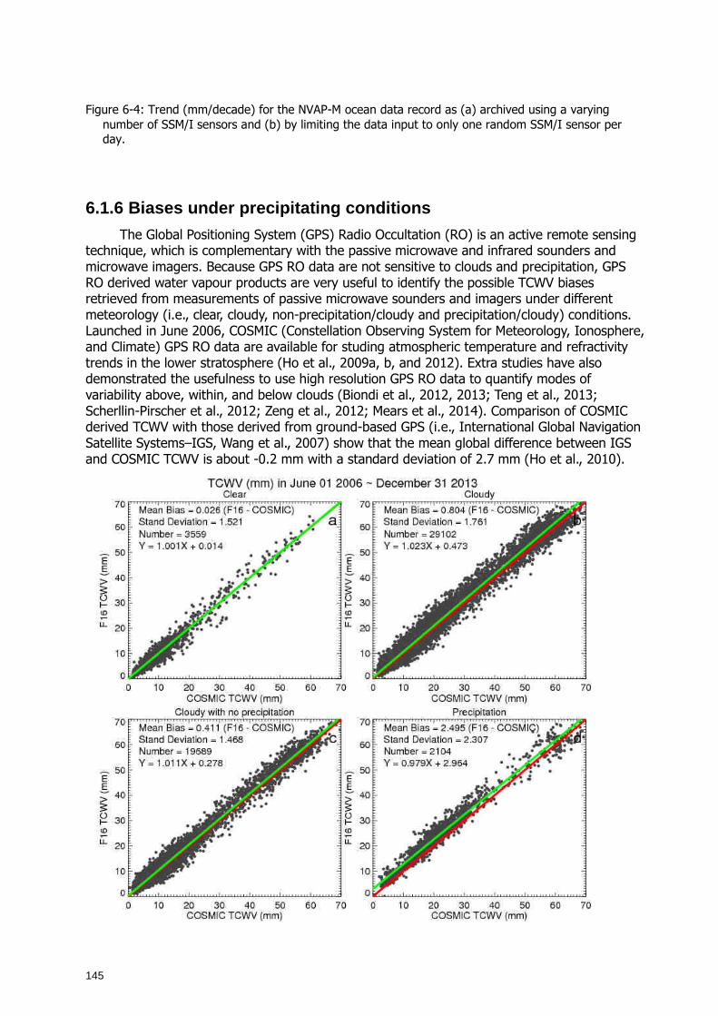
145

Figure 6-4: Trend (mm/decade) for the NVAP-M ocean data record as (a) archived using a varying number of SSM/I sensors and (b) by limiting the data input to only one random SSM/I sensor per day.

6.1.6 Biases under precipitating conditions

The Global Positioning System (GPS) Radio Occultation (RO) is an active remote sensing technique, which is complementary with the passive microwave and infrared sounders and microwave imagers. Because GPS RO data are not sensitive to clouds and precipitation, GPS RO derived water vapour products are very useful to identify the possible TCWV biases retrieved from measurements of passive microwave sounders and imagers under different meteorology (i.e., clear, cloudy, non-precipitation/cloudy and precipitation/cloudy) conditions. Launched in June 2006, COSMIC (Constellation Observing System for Meteorology, Ionosphere, and Climate) GPS RO data are available for studing atmospheric temperature and refractivity trends in the lower stratosphere (Ho et al., 2009a, b, and 2012). Extra studies have also demonstrated the usefulness to use high resolution GPS RO data to quantify modes of variability above, within, and below clouds (Biondi et al., 2012, 2013; Teng et al., 2013; Scherllin-Pirscher et al., 2012; Zeng et al., 2012; Mears et al., 2014). Comparison of COSMIC derived TCWV with those derived from ground-based GPS (i.e., International Global Navigation Satellite Systems–IGS, Wang et al., 2007) show that the mean global difference between IGS and COSMIC TCWV is about -0.2 mm with a standard deviation of 2.7 mm (Ho et al., 2010).

146

Figure 6-5: Scattering plots for the COSMIC and RSS Version 7.0 F16 SSM/I pairs under a) clear, b) cloudy, c) cloudy but non-precipitation, and d) precipitation conditions. COSMIC data with penetration height lower than 0.1 km are included. The water vapour profile below the penetration height is interpolated assuming the relative humidity is equal to 80% where the temperature distribution is interpolated from the temperature of penetration height and surface skin temperature.

Figure 6-5 a-d depict the scattering plots for COSMIC-F16 SSM/I pairs within one hour and 50 km under clear, cloudy (including non-precipitation and precipitation pixels) from June 2006 to Dec. 2013 over oceans (Ho et al., 2016). F16 TCWV daily data in 1440 × 720 grid are downloaded from RSS V7.0 SSM/I ocean products (http://www.remss.com/missions/ssmi). SSM/I TCWV samples for those LWP equal or less than zero are used as clear samples. Under clear condition where SSM/I shall provide high quality TCWV products, the mean TCWV biases between SSM/I and COSMIC (SSM/I – COSMIC) is equal to 0.023 mm with a standard deviation of 1.53 mm. This demonstrates the feasibility of using SSM/I samples for those with LWP less than zero as clear samples. Those F16 pixels with LWP larger than zero are classified as cloudy pixels (Figure 6-5b). Those cloudy pixels with rain rate equal or less than zero are defined as cloudy with no precipitation pixels (Figure 6-5c) and those cloudy with rain rate larger than zero are defined as cloudy with precipitation pixels. Figure 6-5b shows that there are obvious positive TCWV biases mainly resulted from SSM/I retrieval biases (~0.80 mm) under cloudy conditions. Using Figure 6-5d depicts that the large SSM/I TCWV biases are mainly from the pixels under precipitation (mean bias is equal to 2.3 mm) although precipitation pixels are of about less than 6% of the total SSM/I –COSMIC pairs.

6.2 PDF analysis

R. Kursinski (SSE)

6.2.1 Introduction

A fundamental goal in climate research is to measure and understand the water vapour distribution and how it varies across the various spatiotemporal scales of interest across the globe and ultimately how it is controlled so that it can be better modelled and forecast with small uncertainty. Water vapour varies on spatial scales from microscopic to global and temporal scales down to seconds. It must be measured both precisely and accurately, in clear and cloudy conditions, over land and water, creating an, as yet unfulfilled, challenge to characterize it fully.

For climate, water vapour is often characterized in terms of low order statistical moments such as monthly means or standard deviations. This approach provides little indication of the behaviour of moisture extremes which, in many applications, are of primary interest. For instance, the behaviour of humidity near saturation is critical for understanding clouds and precipitation, two very difficult to model variables that are critical to climate. The extreme dry end is also important for radiative cooling of the planet and as a diagnostic of mixing processes in the atmosphere. Furthermore, there are many ways of getting the mean right while getting the distribution wrong, which limits the utility of the moisture mean as a figure of merit in evaluating climate model veracity. It is also important to note that moisture analyses rely on models to vertically distribute the coarse vertical constraints provided by satellite radiance measurements.

147

Because of these issues, we focus here on progress in measuring the Probability Density Function (PDF) of the vertically resolved moisture distribution and its utility in evaluating models and analyses.

6.2.2 Data

The focus here is on PDFs of specific humidity derived from GNSS radio occultations (RO) measurements which are briefly described in Section 3.4 of this report. GNSS RO refractivity profiles provide a unique combination of high precision, accuracy, ~200 meter vertical resolution (with corresponding 100 km horizontal resolution) and insensitivity to clouds and surface emissivity to provide all-weather, global coverage from orbit. Individual profiles of GPS-RO derived moisture extend to approximately the 240 K temperature level in the troposphere. Zonal means extend still higher (e.g., Kursinski and Hajj, 2001). Its 200 m vertical resolution, in both clear and cloudy conditions over land and water with the global perspective from orbit are certainly unique for characterizing and understanding water vapour.

The GPS-RO data record with the largest sampling density to date comes from the 6 satellite COSMIC mission which has provided approximately 10 years of data since its launch in April 2006. As noted in Section 3.4, two methods, referred to as Variational and Direct retrievals, are typically used to extract water vapour information from GPS-RO refractivity profiles. From a climate perspective, the problem with the Variational moisture retrievals is that they include background moisture estimates from numerical weather prediction (NWP) models that likely contain biases. Therefore, our focus here is on the Direct water vapour retrievals which do not make use of background NWP moisture estimates.

GNSS RO is effectively a molecule counter and is therefore sensitive to the amount of water vapour present, rather than the relative humidity. As a result, the water vapour profiles derived from these refractivity profiles extend to higher altitudes in warm, wet conditions. The specific humidity PDFs generated thus far and discussed below contain all of the quality controlled GPS RO profiles measured between 30°S and 30°N over the 2007 annual cycle that extend down to at least 2.5 km altitude. The focus has been low latitudes where moisture concentrations are generally highest and temperature variations are relatively small, conditions that allow one upper altitude bound to be used throughout the annual cycle. The vertical interval extends from 2.5 km to approximately 9 km altitude. While the GPS-RO profiles from the COSMIC mission can extend much closer to the surface than 2.5 km altitude, profiling down into the boundary layer has thus far been avoided in these PDFs because super-refraction occurs in a fraction of GPS-RO profiles that biases the refractivity low in the boundary layer (Xie et al. 2006). As discussed in Section 3.1.2.4, it does appear that the super-refraction problem will be solvable in the near future with better RO instruments.

Kursinski and Gebhardt (2014) (KG14 hereafter) assembled histograms of the low latitude (30°S-30°N), free tropospheric specific humidity from the Direct water vapour retrievals derived from COSMIC refractivity profiles produced at the JPL GPS-RO processing facility. Through an error deconvolution method described in the next section, KG14 determined the 1 sigma uncertainties of the Direct specific humidity shown in Table 6-1. They also estimated that the magnitude of the bias is less than 0.03 g/kg, based on the low end roll-off of the specific humidity PDF at 346 hPa.

Table 6-1: Uncertainties of GPS-RO Direct retrieval specific humidity in the low latitude free troposphere (from Kursinski and Gebhardt, 2014).

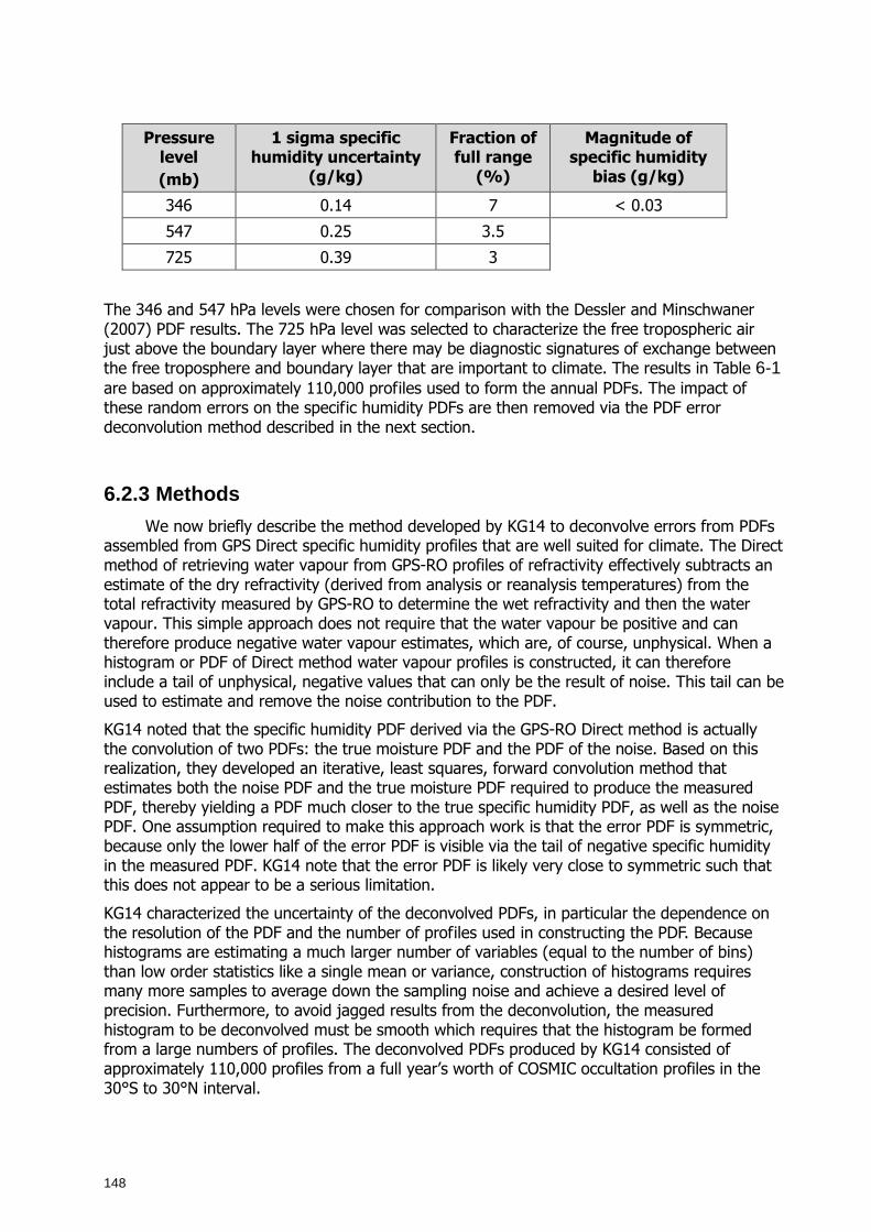
148

Pressure level

(mb)

1 sigma specific humidity uncertainty

(g/kg)

Fraction of full range

(%)

Magnitude of specific humidity

bias (g/kg)

346 0.14 7 < 0.03

547 0.25 3.5

725 0.39 3

The 346 and 547 hPa levels were chosen for comparison with the Dessler and Minschwaner (2007) PDF results. The 725 hPa level was selected to characterize the free tropospheric air just above the boundary layer where there may be diagnostic signatures of exchange between the free troposphere and boundary layer that are important to climate. The results in Table 6-1 are based on approximately 110,000 profiles used to form the annual PDFs. The impact of these random errors on the specific humidity PDFs are then removed via the PDF error deconvolution method described in the next section.

6.2.3 Methods

We now briefly describe the method developed by KG14 to deconvolve errors from PDFs assembled from GPS Direct specific humidity profiles that are well suited for climate. The Direct method of retrieving water vapour from GPS-RO profiles of refractivity effectively subtracts an estimate of the dry refractivity (derived from analysis or reanalysis temperatures) from the total refractivity measured by GPS-RO to determine the wet refractivity and then the water vapour. This simple approach does not require that the water vapour be positive and can therefore produce negative water vapour estimates, which are, of course, unphysical. When a histogram or PDF of Direct method water vapour profiles is constructed, it can therefore include a tail of unphysical, negative values that can only be the result of noise. This tail can be used to estimate and remove the noise contribution to the PDF.

KG14 noted that the specific humidity PDF derived via the GPS-RO Direct method is actually the convolution of two PDFs: the true moisture PDF and the PDF of the noise. Based on this realization, they developed an iterative, least squares, forward convolution method that estimates both the noise PDF and the true moisture PDF required to produce the measured PDF, thereby yielding a PDF much closer to the true specific humidity PDF, as well as the noise PDF. One assumption required to make this approach work is that the error PDF is symmetric, because only the lower half of the error PDF is visible via the tail of negative specific humidity in the measured PDF. KG14 note that the error PDF is likely very close to symmetric such that this does not appear to be a serious limitation.

KG14 characterized the uncertainty of the deconvolved PDFs, in particular the dependence on the resolution of the PDF and the number of profiles used in constructing the PDF. Because histograms are estimating a much larger number of variables (equal to the number of bins) than low order statistics like a single mean or variance, construction of histograms requires many more samples to average down the sampling noise and achieve a desired level of precision. Furthermore, to avoid jagged results from the deconvolution, the measured histogram to be deconvolved must be smooth which requires that the histogram be formed from a large numbers of profiles. The deconvolved PDFs produced by KG14 consisted of approximately 110,000 profiles from a full year’s worth of COSMIC occultation profiles in the 30°S to 30°N interval.

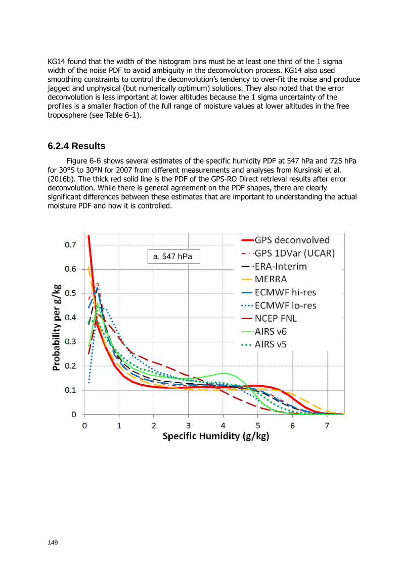
149

KG14 found that the width of the histogram bins must be at least one third of the 1 sigma width of the noise PDF to avoid ambiguity in the deconvolution process. KG14 also used smoothing constraints to control the deconvolution’s tendency to over-fit the noise and produce jagged and unphysical (but numerically optimum) solutions. They also noted that the error deconvolution is less important at lower altitudes because the 1 sigma uncertainty of the profiles is a smaller fraction of the full range of moisture values at lower altitudes in the free troposphere (see Table 6-1).

6.2.4 Results

Figure 6-6 shows several estimates of the specific humidity PDF at 547 hPa and 725 hPa for 30°S to 30°N for 2007 from different measurements and analyses from Kursinski et al. (2016b). The thick red solid line is the PDF of the GPS-RO Direct retrieval results after error deconvolution. While there is general agreement on the PDF shapes, there are clearly significant differences between these estimates that are important to understanding the actual moisture PDF and how it is controlled.

a. 547 hPa

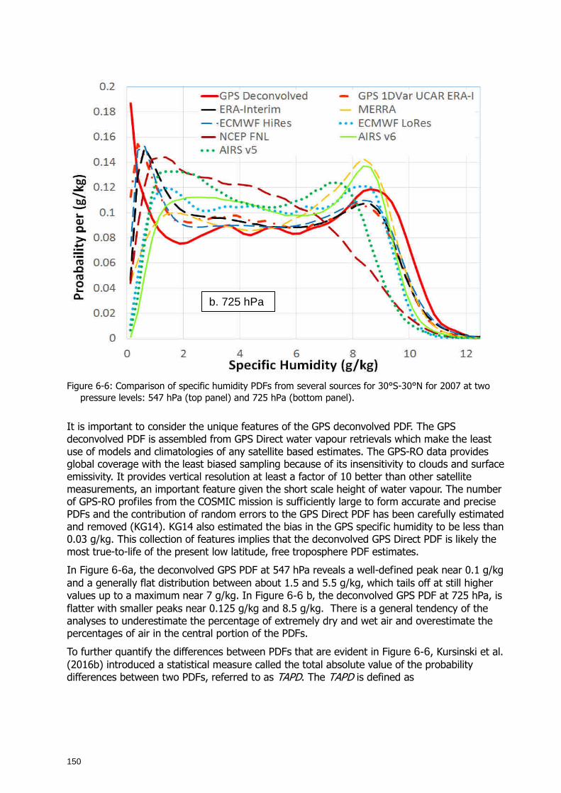
150

Figure 6-6: Comparison of specific humidity PDFs from several sources for 30°S-30°N for 2007 at two

pressure levels: 547 hPa (top panel) and 725 hPa (bottom panel).

It is important to consider the unique features of the GPS deconvolved PDF. The GPS deconvolved PDF is assembled from GPS Direct water vapour retrievals which make the least use of models and climatologies of any satellite based estimates. The GPS-RO data provides global coverage with the least biased sampling because of its insensitivity to clouds and surface emissivity. It provides vertical resolution at least a factor of 10 better than other satellite measurements, an important feature given the short scale height of water vapour. The number of GPS-RO profiles from the COSMIC mission is sufficiently large to form accurate and precise PDFs and the contribution of random errors to the GPS Direct PDF has been carefully estimated and removed (KG14). KG14 also estimated the bias in the GPS specific humidity to be less than 0.03 g/kg. This collection of features implies that the deconvolved GPS Direct PDF is likely the most true-to-life of the present low latitude, free troposphere PDF estimates.

In Figure 6-6a, the deconvolved GPS PDF at 547 hPa reveals a well-defined peak near 0.1 g/kg and a generally flat distribution between about 1.5 and 5.5 g/kg, which tails off at still higher values up to a maximum near 7 g/kg. In Figure 6-6 b, the deconvolved GPS PDF at 725 hPa, is flatter with smaller peaks near 0.125 g/kg and 8.5 g/kg. There is a general tendency of the analyses to underestimate the percentage of extremely dry and wet air and overestimate the percentages of air in the central portion of the PDFs.

To further quantify the differences between PDFs that are evident in Figure 6-6, Kursinski et al. (2016b) introduced a statistical measure called the total absolute value of the probability differences between two PDFs, referred to as TAPD. The TAPD is defined as

b. 725 hPa

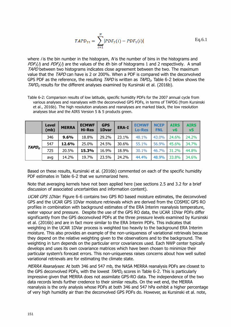
151

Eq. 6.1

where i is the bin number in the histogram, N is the number of bins in the histograms and PDF1(i) and PDF2(i) are the values of the ith bin of histograms 1 and 2 respectively. A small TAPD between two histograms indicates close agreement between the two. The maximum value that the TAPD can have is 2 or 200%. When a PDF is compared with the deconvolved GPS PDF as the reference, the resulting TAPD is written as TAPDG. Table 6-2 below shows the TAPDG results for the different analyses examined by Kursinski et al. (2016b).

Table 6-2: Comparison results of low latitude, specific humidity PDFs for the 2007 annual cycle from various analyses and reanalyses with the deconvolved GPS PDFs, in terms of TAPDG (from Kursinski et al., 2016b). The high resolution analyses and reanalyses are marked black, the low resolution analyses blue and the AIRS Version 5 & 5 products green.

Level

(mb) MERRA

ECMWF

Hi-Res

GPS

1Dvar ERA-I

ECMWF

Lo-Res

NCEP

FNL

AIRS

v6

AIRS

v5

TAPDG

346 9.6% 18.8% 29.2% 23.1% 48.1% 43.0% 24.6% 24.2%

547 12.6% 25.0% 24.5% 30.6% 55.1% 56.9% 45.6% 34.7%

725 20.5% 15.3% 16.9% 18.9% 30.1% 46.7% 31.2% 44.8%

avg 14.2% 19.7% 23.5% 24.2% 44.4% 48.9% 33.8% 34.6%

Based on these results, Kursinski et al. (2016b) commented on each of the specific humidity PDF estimates in Table 6-2 that we summarized here.

Note that averaging kernels have not been applied here (see sections 2.5 and 3.2 for a brief discussion of associated uncertainties and information content).

UCAR GPS 1DVar: Figure 6-6 contains two GPS RO based moisture estimates, the deconvolved GPS and the UCAR GPS 1DVar moisture retrievals which are derived from the COSMIC GPS RO profiles in combination with background estimates of the ERA Interim reanalysis temperature, water vapour and pressure. Despite the use of the GPS RO data, the UCAR 1DVar PDFs differ significantly from the GPS deconvolved PDFs at the three pressure levels examined by Kursinski et al. (2016b) and are in fact more similar to the ERA Interim PDFs. This indicates that weighting in the UCAR 1DVar process is weighted too heavily to the background ERA Interim moisture. This also provides an example of the non-uniqueness of variational retrievals because they depend on the relative weighting given to the observations and to the background. The weighting in turn depends on the particular error covariances used. Each NWP center typically develops and uses its own covariance matrices which have been chosen to minimize their particular system’s forecast errors. This non-uniqueness raises concerns about how well suited variational retrievals are for estimating the climate state.

MERRA Reanalyses: At both 346 and 547 mb, the NASA MERRA reanalysis PDFs are closest to the GPS deconvolved PDFs, with the lowest TAPDG scores in Table 6-2. This is particularly impressive given that MERRA does not assimilate GPS-RO data. The independence of the two data records lends further credence to their similar results. On the wet end, the MERRA reanalysis is the only analysis whose PDFs at both 346 and 547 hPa exhibit a higher percentage of very high humidity air than the deconvolved GPS PDFs do. However, as Kursinski et al. note,

152

the MERRA means are a bit high which may indicate that these higher than GPS deconvolved percentages at the extreme high end of the distribution are overestimated. At 725 hPa, the MERRA PDF is less realistic, with percentages of moist air between 5 and 9 g/kg that are substantially too high and percentages of very dry air that are substantially too low, again, in comparison with the GPS deconvolved PDF. These errors suggest that there is too much exchange in the MERRA reanalyses between the boundary layer and the free troposphere.

ECMWF high resolution analyses: The PDFs of the ECMWF high resolution operational analyses are similar to those of GPS deconvolved, coming in second to MERRA in Table 6-2, but they do underestimate the percentages of both the driest and the wettest air. At 725 hPa, the Hi-Res ECMWF PDF is the most similar to the deconvolved GPS PDF (see Table 6-2) but slightly underestimates the fraction of the wettest air and misses the relative maximum at the extreme dry end of the distribution, as do all of the estimates other than the deconvolved GPS.

ERA Interim: The ERA Interim PDFs are quite similar to and slightly worse than the PDFs from the full resolution ECMWF analyses. This is not surprising because the ERA Interim analysis system is essentially the ECMWF operational NWP system as of the end of 2006 except that it is run at lower horizontal and vertical resolutions which are factors of approximately 3 and 1.4 times lower respectively than the full resolution ECMWF analyses in 2007. Thus, at least in 2007, ERA Interim reanalyses are not too much worse than the full resolution ECMWF operational analyses which are useful news for researchers using these reanalyses. This does raise the question of how much better the full resolution operational analyses have become since the 2007 analyses examined here.

ECMWF low resolution analyses: This freely available, low resolution product is produced by ECMWF by interpolating the high resolution analyses to lower vertical and horizontal resolutions. Interpolation is an averaging process that reduces extremes as is readily apparent in Figure 6-6 in the compression of the moisture distribution and reduction of the percentages of wet and dry extremes in the ECMWF low resolution PDFs in comparison to the ECMWF high resolution analysis PDFs. As a result, interpreting the shape of the low resolution analysis PDF would lead one to deduce that atmospheric diffusion and mixing are stronger than what occurs in reality. Thus, researchers must use low resolution analysis products with care and not overly interpret their apparent behaviour.

NCEP FNL analyses: Of the analysis PDFs examined by Kursinski et al. (2016b), the PDFs from the NCEP FNL analyses generally differ more from the GPS Direct PDFs than any other estimate, with too little air with extremely high and low moisture concentrations, and too much air with medium humidity amounts. Given that these results are for 2007, it would be interesting to examine more recent NCEP analyses at their full resolution to assess their present level of realism.

AIRS Level 3 products: PDFs from both Versions 5 and 6 of the AIRS Level 3 products are shown in Figure 6-6. At 346 mb, the two versions are about the same. At 547 mb, Version 5 is closer to the deconvolved GPS and at 725 mb, Version 6 is closer. However, both versions significantly underestimate the percentages of extremely wet and dry air, which causes their TAPDG scores to be relatively high. At 725 mb, Version 6 is better than Version 5 due primarily to Version 6’s significantly better representation of the wet end of the moisture distribution. The improvement in the Version 6 retrievals across the wet portion of the distribution at 725 mb is apparently due to a first guess based on a neural network trained by recent ECMWF. However, the Version 6 PDF at 547 mb also exhibits a peak near 4 g/kg and rapid falloff at higher specific humidities that none of the other analyses exhibit which produces a particularly poor TAPDG score there. Both versions underestimate the percentage of dry air at 725 mb which is likely due to the coarse, ~2 km vertical resolution of the IR averaging kernels which smear out the sharp vertical transition between the moist boundary layer and drier overlying

153

free troposphere, limiting the ability to detect the presence of extremely dry free tropospheric air just above the boundary layer.

6.2.5 Conclusions

Value of GPS RO Direct retrievals + deconvolution: GNSS RO provides a unique combination of globally distributed, 200 m vertical resolution, high precision and accuracy, all-weather profiling of free tropospheric water vapour up to about the 240 K level in the troposphere. A good understanding of the uncertainties in the GPS-RO Direct retrieval water vapour results has been developed that suggests that GPS-RO is the least biased water vapour data record in the free troposphere up to the altitudes to which it can profile moisture.

PDFs: PDFs provide a far more stringent quantification of the moisture distribution than do low order statistical moments like the mean and variance. The number of occultation profiles from the 9 year COSMIC mission is sufficient that PDFs can be formed from GPS-RO results. A deconvolution method has been developed to estimate and remove random errors from GPS Direct PDFs which has been used to construct annual histograms for 30°S-30°N in the free troposphere. Detailed examination of the uncertainties indicates the resulting histograms are quite accurate. Also worthy of note is the fact that the deconvolution of the GPS Direct PDF is less important at lower altitudes where the width of the error PDF is a smaller fraction of the full range of the specific humidity PDF at lower altitudes in the free troposphere.

Overall Comparison Summary: Figure 6-7 shows a summary of the range of TAPDG values from Kursinski et al. (2016b) at the three pressure levels they examined, 346, 547 and 725 mb, representing the lower, middle and upper free troposphere. TAPDG ranges for several classes of PDF estimates are shown. The high resolution analyses which are the MERRA and ERA Interim reanalyses, the full resolution ECWMF analyses and the UCAR 1DVar GPS results score the best overall. The low resolution analyses are the low resolution ECMWF and the NCEP FNL operational analyses which score rather poorly. The AIRS Versions 5 and 6 are shown and score in the middle. The climate models examined are divided between CMIP5 and CMIP3 models and show a rather wide range of scores. The simple advection-saturation model of Dessler and Minschwaner (2007) is also shown and labelled as “Adv-sat” at the 346 and 547 mb levels.

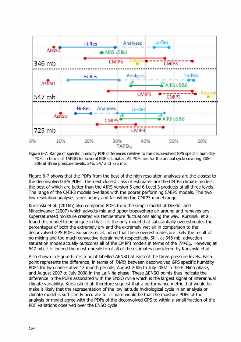
154

Figure 6-7: Range of specific humidity PDF differences relative to the deconvolved GPS specific humidity PDFs in terms of TAPDG for several PDF estimates. All PDFs are for the annual cycle covering 30S-30N at three pressure levels, 346, 547 and 725 mb.

Figure 6-7 shows that the PDFs from the best of the high resolution analyses are the closest to the deconvolved GPS PDFs. The next closest class of estimates are the CMIP5 climate models, the best of which are better than the AIRS Version 5 and 6 Level 3 products at all three levels. The range of the CMIP3 models overlaps with the poorer performing CMIP5 models. The two low resolution analyses score poorly and fall within the CMIP3 model range.

Kursinski et al. (2016b) also compared PDFs from the simple model of Dessler and Minschwaner (2007) which advects mid and upper troposphere air around and removes any supersaturated moisture created via temperature fluctuations along the way. Kursinski et al. found this model to be unique in that it is the only model that substantially overestimates the percentages of both the extremely dry and the extremely wet air in comparison to the deconvolved GPS PDFs. Kursinski et al. noted that these overestimates are likely the result of no mixing and too much convective detrainment respectively. Still, at 346 mb, advection-saturation model actually outscores all of the CMIP3 models in terms of the TAPDG. However, at 547 mb, it is indeed the most unrealistic of all of the estimates considered by Kursinski et al.

Also shown in Figure 6-7 is a point labelled ∆ENSO at each of the three pressure levels. Each point represents the difference, in terms of TAPD, between deconvolved GPS specific humidity PDFs for two consecutive 12 month periods, August 2006 to July 2007 in the El Niño phase, and August 2007 to July 2008 in the La Niña phase. These ∆ENSO points thus indicate the difference in the PDFs associated with the ENSO cycle which is the largest signal of interannual climate variability. Kursinski et al. therefore suggest that a performance metric that would be make it likely that the representation of the low latitude hydrological cycle in an analysis or climate model is sufficiently accurate for climate would be that the moisture PDFs of the analysis or model agree with the PDFs of the deconvolved GPS to within a small fraction of the PDF variations observed over the ENSO cycle.

155

In this regard, Figure 6-7 shows that, as of 2007, the differences between even the best of the high resolution analyses and the deconvolved GPS PDFs are larger than the changes associated with ENSO’s large year to year variations as captured by the deconvolved GPS PDFs which indicates there is substantial need for improvement among the analyses and even more so for the climate models.

Importance of resolution: Comparison of PDFs from the ECMWF high resolution and low resolution analyses shows that interpolation to lower resolution significantly distorts and compresses the PDF. Thus, any moisture analysis-based research on the hydrological cycle should use the highest resolution analysis products available (which are still not correct but definitely better than lower resolution products).

While model and analysis resolution are clearly important, the similarity of the ECMWF full resolution analyses and the ERA-Interim reanalyses, despite the lower resolution of the ERA-Interim reanalyses (by factors of 1.4 (vertical) and 3 (horizontal) relative to the full resolution ECMWF analyses) indicates that the model’s dynamics, physics and parameterizations are very important as well.

Utility of Versions 5 and 6 of the AIRS Level 3 products: Based on the results summary in Figure 6-7, the AIRS Versions 5 & 6 are less realistic than the high resolution analyses and reanalyses and the best of the climate models. This raises questions about their utility for evaluating model realism and providing guidance to model developers.

Constraints on Processes: Observations are critical for providing constraints on the important processes operating in the atmosphere that modelers need to guide them in order to improve the realism and predictive skill of their models. The consistent underestimate of percentage of extremely dry air by the analyses (see Figure 6-6) and even more so in the climate models (Kursinski et al., 2016b) suggests there is too much mixing in the models. This further suggests that the positive water vapor feedback in models is overestimated.

Accurate representation of clouds and precipitation is very challenging for models. The PDF comparisons reveal that all of the climate models and all but one reanalyses underestimate the percentage of extremely wet air. Since this is a requirement for realistic clouds and precipitation, the information provided by these PDFs will hopefully help provide some guidance to modelers in this area.

An important issue in climate is the exchange of moisture between the boundary layer and overlying free troposphere which is tied closely to cloud albedo, a critically important feedback with a large uncertainty. Based on comparing climate models with the MERRA and ERA Interim reanalyses, Sherwood et al. (2014) concluded that the models with more exchange between the boundary layer and free troposphere are more realistic and therefore, the rise in surface temperatures due to anthropogenic climate change will be in the upper half of the range of climate model predictions.

However, the PDF comparisons with the deconvolved GPS results at 725 mb suggest that the CMIP5 models are overestimating that exchange of moisture and therefore the Sherwood et al. conclusion may be incorrect.

Structural uncertainty: The specific humidity PDF figures and tabular TAPD results shown above reveal a substantial spread across the PDFs from the various high resolution analyses and reanalyses and AIRS Version 5 and 6 products. This spread exists even though each of these estimates has used or assimilated the enormous volume of globally distributed radiance observations from satellites, including the AIRS hyperspectral IR radiances.

This spread can therefore be interpreted as the structural uncertainty of vertically resolved specific humidity derived using satellite radiances, model analyses and reanalyses. Structural

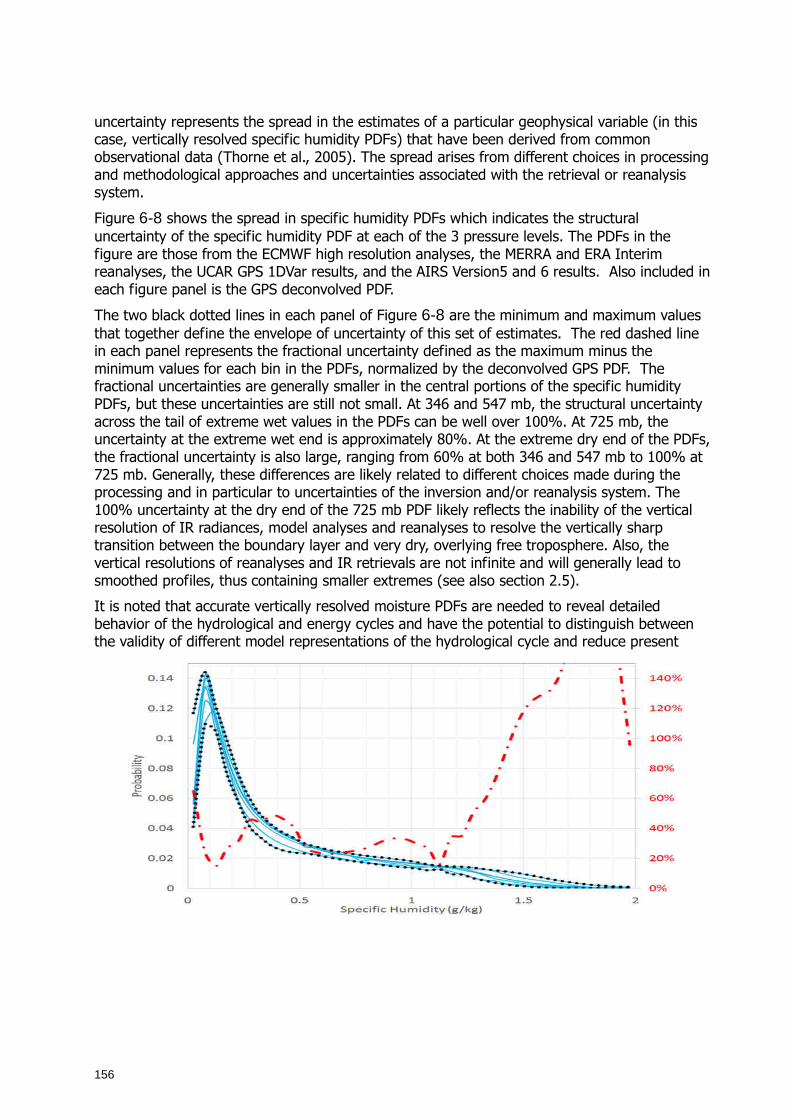
156

uncertainty represents the spread in the estimates of a particular geophysical variable (in this case, vertically resolved specific humidity PDFs) that have been derived from common observational data (Thorne et al., 2005). The spread arises from different choices in processing and methodological approaches and uncertainties associated with the retrieval or reanalysis system.

Figure 6-8 shows the spread in specific humidity PDFs which indicates the structural uncertainty of the specific humidity PDF at each of the 3 pressure levels. The PDFs in the figure are those from the ECMWF high resolution analyses, the MERRA and ERA Interim reanalyses, the UCAR GPS 1DVar results, and the AIRS Version5 and 6 results. Also included in each figure panel is the GPS deconvolved PDF.

The two black dotted lines in each panel of Figure 6-8 are the minimum and maximum values that together define the envelope of uncertainty of this set of estimates. The red dashed line in each panel represents the fractional uncertainty defined as the maximum minus the minimum values for each bin in the PDFs, normalized by the deconvolved GPS PDF. The fractional uncertainties are generally smaller in the central portions of the specific humidity PDFs, but these uncertainties are still not small. At 346 and 547 mb, the structural uncertainty across the tail of extreme wet values in the PDFs can be well over 100%. At 725 mb, the uncertainty at the extreme wet end is approximately 80%. At the extreme dry end of the PDFs, the fractional uncertainty is also large, ranging from 60% at both 346 and 547 mb to 100% at 725 mb. Generally, these differences are likely related to different choices made during the processing and in particular to uncertainties of the inversion and/or reanalysis system. The 100% uncertainty at the dry end of the 725 mb PDF likely reflects the inability of the vertical resolution of IR radiances, model analyses and reanalyses to resolve the vertically sharp transition between the boundary layer and very dry, overlying free troposphere. Also, the vertical resolutions of reanalyses and IR retrievals are not infinite and will generally lead to smoothed profiles, thus containing smaller extremes (see also section 2.5).

It is noted that accurate vertically resolved moisture PDFs are needed to reveal detailed behavior of the hydrological and energy cycles and have the potential to distinguish between the validity of different model representations of the hydrological cycle and reduce present

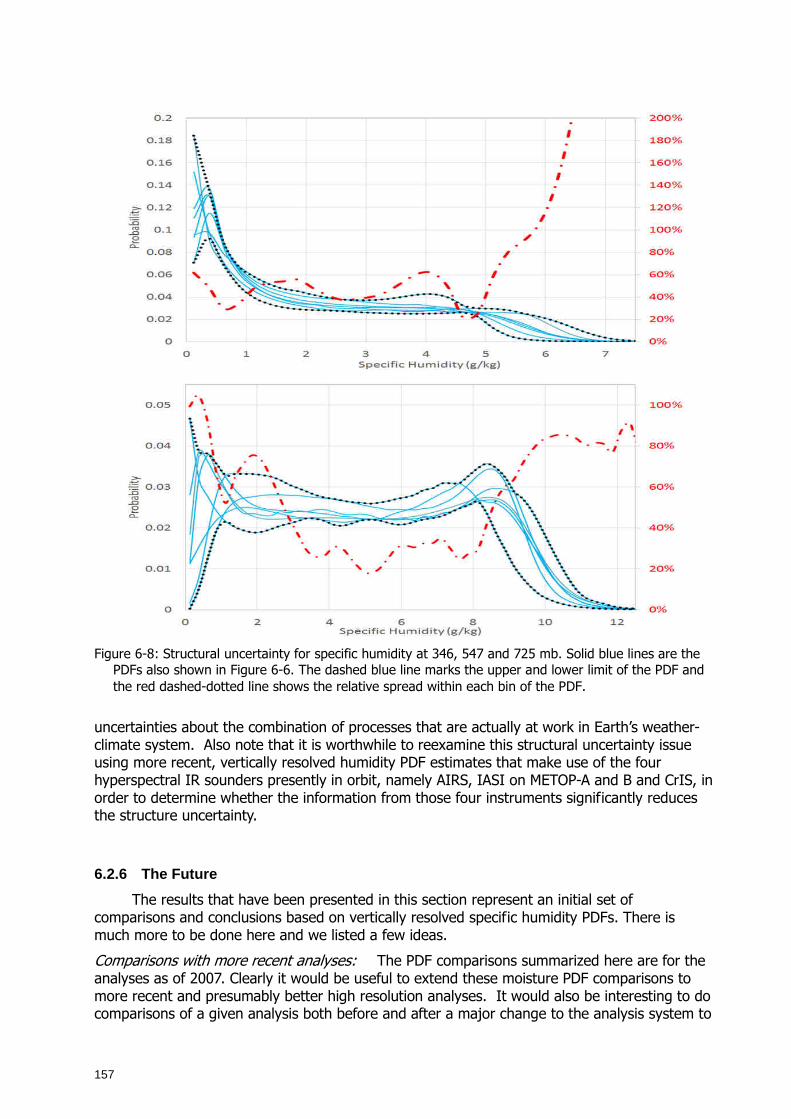
157

Figure 6-8: Structural uncertainty for specific humidity at 346, 547 and 725 mb. Solid blue lines are the

PDFs also shown in Figure 6-6. The dashed blue line marks the upper and lower limit of the PDF and the red dashed-dotted line shows the relative spread within each bin of the PDF.

uncertainties about the combination of processes that are actually at work in Earth’s weather-climate system. Also note that it is worthwhile to reexamine this structural uncertainty issue using more recent, vertically resolved humidity PDF estimates that make use of the four hyperspectral IR sounders presently in orbit, namely AIRS, IASI on METOP-A and B and CrIS, in order to determine whether the information from those four instruments significantly reduces the structure uncertainty.

6.2.6 The Future

The results that have been presented in this section represent an initial set of comparisons and conclusions based on vertically resolved specific humidity PDFs. There is much more to be done here and we listed a few ideas.

Comparisons with more recent analyses: The PDF comparisons summarized here are for the analyses as of 2007. Clearly it would be useful to extend these moisture PDF comparisons to more recent and presumably better high resolution analyses. It would also be interesting to do comparisons of a given analysis both before and after a major change to the analysis system to

158

determine how its moisture PDF performance changes.

Relative humidity: While the PDF deconvolution method has been applied only to specific humidity, an analogous PDF deconvolution method is being developed for relative humidity that will be useful particularly for better understanding behavior and issues associated with high relative humidity conditions particularly given the unique capabilities of GPS RO to routinely peer into and vertically resolve these regions across the globe.

Smaller temporal and spatial domains: KG14 showed that accurate deconvolved histograms can be created from as few as 10,000 profiles which enable PDFs to be created for smaller spatiotemporal domains in order to resolve and separate behaviour over the seasons and regions of rising and sinking air at low latitudes. Furthermore, the number of GNSS RO occultations should increase dramatically over the next few years, beginning with a factor of 5 increase in low latitude sampling with the 6 satellite COSMIC-2 equatorial GNSS RO mission scheduled to launch in 2017. Several companies have announced plans to launch satellite constellation generating GNSS RO data as well. If that data is of sufficient quality, it will enable PDFs to be generated for still smaller spatiotemporal domains in the future. More research is needed to decide what additional products to make standard on regional scales and seasonal and shorter temporal scales. Doing so and regularly producing these standard products will require funding which has been in limited supply for this work.

Boundary layer: While the results generated thus far have been restricted to the free troposphere because of a negative bias in warm wet boundary layers associated with super-refraction (see Section 3.1.2.4), it appears that this present limitation may be overcome with the better GNSS RO receivers on COSMIC-2 that promise the ability to profile the low latitude boundary layer beginning in late 2016.

Increase the GNSS RO Impact: Another point is related to the impact of GPS RO on NWP moisture analyses. Development of methods to assimilate GPS-RO data into global NWP systems began at least 15 years ago (e.g., Healy and Eyre, 2000) and GPS-RO data is now being routinely assimilated into many global NWP analyses. Harnisch et al. (2013) simulated the impact of large numbers of GNSS occultations up to 128,000 per day and predicted that GNSS RO will have a large impact on the moisture analyses when the numbers of occultations become much larger than they are at present. Thus, we anticipate that as the number of GNSS occultation increases, the moisture analyses from NWP systems will capture that information and become more accurate and useful for climate.

ATOMMS occultations near water vapor absorption lines: While GPS RO has a number of unique features, it has limited ability to profile water vapor in the winter hemisphere and uppermost troposphere and above, and requires using analyzed temperatures to isolate the water vapor. As described briefly in Section 3.1.2.4, a major advance in the global observing capability and understanding would be enabled via satellite to satellite occultations near the 22 and 183 GHz water vapor absorption lines. Such a system, called ATOMMS, will extend the features of GPS RO by profiling water vapor and temperature simultaneously (avoiding the dependence on models or analyses), with 100 m vertical resolution, and will likely achieve ~1% water vapor precision and accuracy with a dynamic range from lower troposphere into the mesosphere, in clear and cloudy air. As noted in Kursinski et al. (2016a) and the references therein, mountaintop measurements have demonstrated ATOMMS ability to measure water vapor to better than 1% in optical depths up to 17 (7 orders of magnitude attenuation) and the sampling densities needed for weather and climate can be achieved by implementing this system on a constellation of very small satellites.

159

6.3 Collocation

X. Calbet (AEMET), H. Brogniez (U. Versailles/LATMOS), S. Crewell (U. Cologne), S. Eikenberg (U. Cologne), J. Kinzel (DWD), M. Schröder (DWD), B. Sun (NOAA/NESDIS/STAR & IMSG), S. Steinke (U. Cologne), T. Trent (U. Leicester)

Space-borne instruments are ideal for monitoring climate variables thanks to their ability to provide a global and continuous coverage of these data records. They have, however, limited accuracy, low vertical resolution and relatively high footprint sizes. The reason for this is that the instruments on board of satellites are mostly based on passive remote sensing. This implies that what is directly measured are emitted radiances, from which the climate variables are indirectly inferred, having as a consequence lower accuracy and resolution, which is not always what is necessary for climate applications as stated in GCOS-154 or Wulfmeyer et al. (2015).

On the other hand, ground based instruments can provide high vertical and horizontal spatial resolution and accuracy. One of such examples are radiosondes (e.g Miloshevich et al. 2006). Another kind of ground-based instruments are the remote sensing ones that also provide a high temporal sampling (e.g. Wulfmeyer et al. 2015). However, one of their main drawbacks is the limitation in the number of sites that prevents them from having a global coverage. They also require frequent maintenance that can limit the temporal coverage.

The synergy between both, space-borne and ground based measurements, would be ideal to measure such an important parameter for climate like water vapor concentration in the atmosphere. While space-borne instruments provide global coverage, ground based measurements provide the anchoring point of these measurements by means of validating and calibrating the space sensors. Ground based instruments would also provide added value to the water vapour measurements such as their high resolution and accuracy, which is currently not available from satellites.

The synergistic approach is not as straightforward as it may seem at first sight. The main reason for this is that although both systems might be observing the same region of the atmosphere, they are actually not measuring exactly the same air parcel. Satellite footprint sizes are provided in Table 3-2 and range from 0.25 km x 0.25 km to 40 km x 320 km, while the horizontal scale of ground based remote sensing instruments is of the order of a few meters and radiosondes provide an almost point-like observation. Vertical scales are also very different, ranging from a few kilometers for the vertical resolution of satellite based passive remote sensing instruments to a few meters or centimeters for some ground-based ones. On the temporal scales, satellites usually provide a near instantaneous measurement of a complete column of the atmosphere while ground-based instruments measurements take from a few minutes (e.g. LIDARs at the lower troposphere) to over one or even several hours (e.g. radiosondes or LIDARS at the high troposphere). These huge differences in the air parcels, when measuring the same region of the atmosphere by satellite and ground based instruments, form what is known as the collocation problem. The net effect is that there will always be a mismatch between the measurements made by a satellite instrument and by a ground based one when observing the same region of the atmosphere at similar times. The key element here is that although both measurements are made in different ways they should be consistent or compatible. Two measurements from different instruments are consistent, if the measurement differences statistically lie within the combined uncertainty of the measurements and the collocation uncertainty (see also section 3.2). For the case of water vapour, the collocation uncertainty between two atmospheric measurements can be quite large, even when both measurements are performed relatively

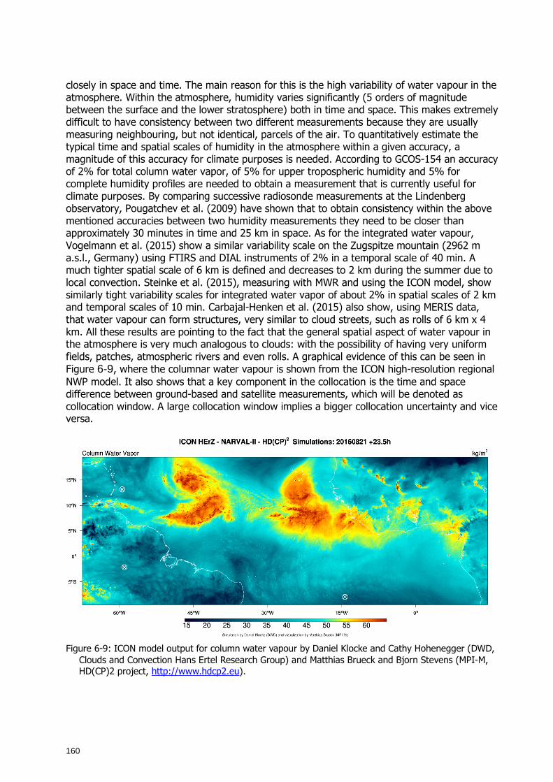
160

closely in space and time. The main reason for this is the high variability of water vapour in the atmosphere. Within the atmosphere, humidity varies significantly (5 orders of magnitude between the surface and the lower stratosphere) both in time and space. This makes extremely difficult to have consistency between two different measurements because they are usually measuring neighbouring, but not identical, parcels of the air. To quantitatively estimate the typical time and spatial scales of humidity in the atmosphere within a given accuracy, a magnitude of this accuracy for climate purposes is needed. According to GCOS-154 an accuracy of 2% for total column water vapor, of 5% for upper tropospheric humidity and 5% for complete humidity profiles are needed to obtain a measurement that is currently useful for climate purposes. By comparing successive radiosonde measurements at the Lindenberg observatory, Pougatchev et al. (2009) have shown that to obtain consistency within the above mentioned accuracies between two humidity measurements they need to be closer than approximately 30 minutes in time and 25 km in space. As for the integrated water vapour, Vogelmann et al. (2015) show a similar variability scale on the Zugspitze mountain (2962 m a.s.l., Germany) using FTIRS and DIAL instruments of 2% in a temporal scale of 40 min. A much tighter spatial scale of 6 km is defined and decreases to 2 km during the summer due to local convection. Steinke et al. (2015), measuring with MWR and using the ICON model, show similarly tight variability scales for integrated water vapor of about 2% in spatial scales of 2 km and temporal scales of 10 min. Carbajal-Henken et al. (2015) also show, using MERIS data, that water vapour can form structures, very similar to cloud streets, such as rolls of 6 km x 4 km. All these results are pointing to the fact that the general spatial aspect of water vapour in the atmosphere is very much analogous to clouds: with the possibility of having very uniform fields, patches, atmospheric rivers and even rolls. A graphical evidence of this can be seen in Figure 6-9, where the columnar water vapour is shown from the ICON high-resolution regional NWP model. It also shows that a key component in the collocation is the time and space difference between ground-based and satellite measurements, which will be denoted as collocation window. A large collocation window implies a bigger collocation uncertainty and vice versa.

Figure 6-9: ICON model output for column water vapour by Daniel Klocke and Cathy Hohenegger (DWD,

Clouds and Convection Hans Ertel Research Group) and Matthias Brueck and Bjorn Stevens (MPI-M, HD(CP)2 project, http://www.hdcp2.eu).

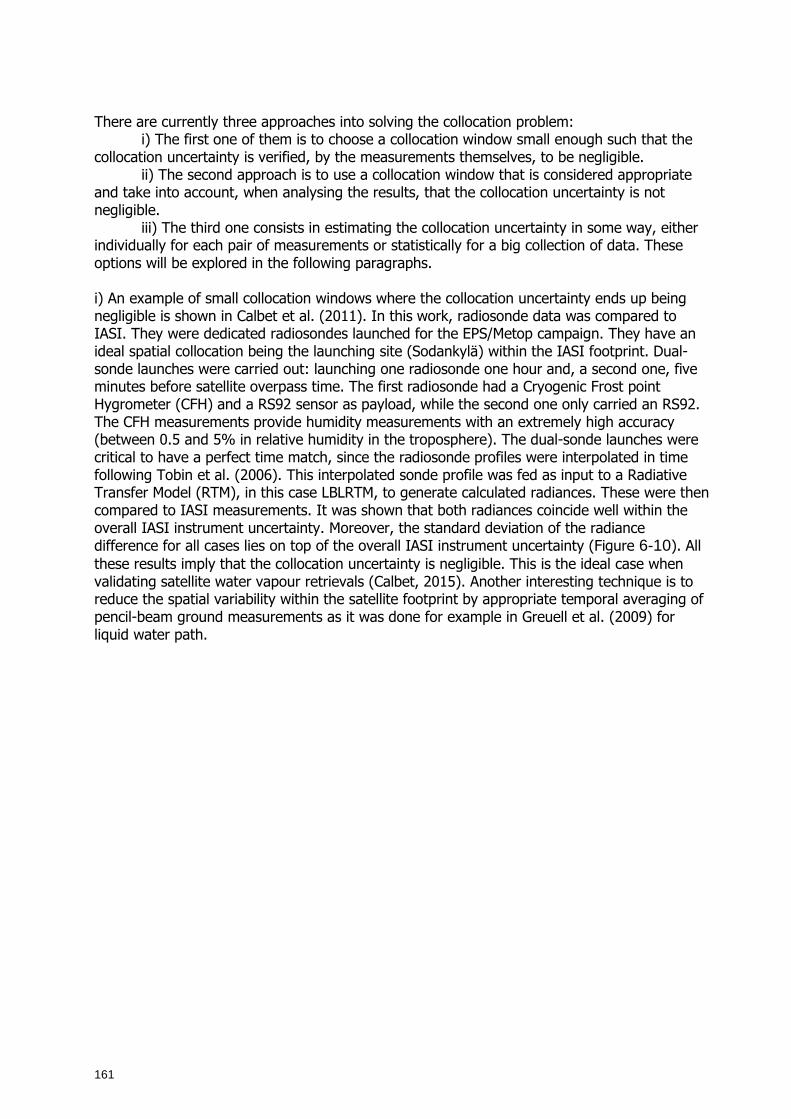
161

There are currently three approaches into solving the collocation problem: i) The first one of them is to choose a collocation window small enough such that the

collocation uncertainty is verified, by the measurements themselves, to be negligible. ii) The second approach is to use a collocation window that is considered appropriate

and take into account, when analysing the results, that the collocation uncertainty is not negligible.

iii) The third one consists in estimating the collocation uncertainty in some way, either individually for each pair of measurements or statistically for a big collection of data. These options will be explored in the following paragraphs. i) An example of small collocation windows where the collocation uncertainty ends up being negligible is shown in Calbet et al. (2011). In this work, radiosonde data was compared to IASI. They were dedicated radiosondes launched for the EPS/Metop campaign. They have an ideal spatial collocation being the launching site (Sodankylä) within the IASI footprint. Dual-sonde launches were carried out: launching one radiosonde one hour and, a second one, five minutes before satellite overpass time. The first radiosonde had a Cryogenic Frost point Hygrometer (CFH) and a RS92 sensor as payload, while the second one only carried an RS92. The CFH measurements provide humidity measurements with an extremely high accuracy (between 0.5 and 5% in relative humidity in the troposphere). The dual-sonde launches were critical to have a perfect time match, since the radiosonde profiles were interpolated in time following Tobin et al. (2006). This interpolated sonde profile was fed as input to a Radiative Transfer Model (RTM), in this case LBLRTM, to generate calculated radiances. These were then compared to IASI measurements. It was shown that both radiances coincide well within the overall IASI instrument uncertainty. Moreover, the standard deviation of the radiance difference for all cases lies on top of the overall IASI instrument uncertainty (Figure 6-10). All these results imply that the collocation uncertainty is negligible. This is the ideal case when validating satellite water vapour retrievals (Calbet, 2015). Another interesting technique is to reduce the spatial variability within the satellite footprint by appropriate temporal averaging of pencil-beam ground measurements as it was done for example in Greuell et al. (2009) for liquid water path.

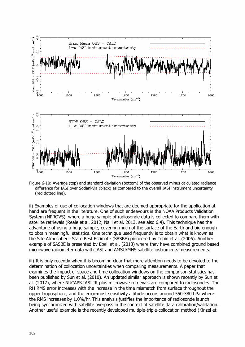
162

Figure 6-10: Average (top) and standard deviation (bottom) of the observed minus calculated radiance

difference for IASI over Sodänkyla (black) as compared to the overall IASI instrument uncertainty (red dotted line).

ii) Examples of use of collocation windows that are deemed appropriate for the application at hand are frequent in the literature. One of such endeavours is the NOAA Products Validation System (NPROVS), where a huge sample of radiosonde data is collected to compare them with satellite retrievals (Reale et al. 2012; Nalli et al. 2013, see also 6.4). This technique has the advantage of using a huge sample, covering much of the surface of the Earth and big enough to obtain meaningful statistics. One technique used frequently is to obtain what is known as the Site Atmospheric State Best Estimate (SASBE) pioneered by Tobin et al. (2006). Another example of SASBE is presented by Ebell et al. (2013) where they have combined ground based microwave radiometer data with IASI and AMSU/MHS satellite instruments measurements. iii) It is only recently when it is becoming clear that more attention needs to be devoted to the determination of collocation uncertainties when comparing measurements. A paper that examines the impact of space and time collocation windows on the comparison statistics has been published by Sun et al. (2010). An updated similar approach is shown recently by Sun et al. (2017), where NUCAPS IASI IR plus microwave retrievals are compared to radiosondes. The RH RMS error increases with the increase in the time mismatch from surface throughout the upper troposphere, and the error-most sensitivity altitude occurs around 550-380 hPa where the RMS increases by 1.0%/hr. This analysis justifies the importance of radiosonde launch being synchronized with satellite overpass in the context of satellite data calibration/validation. Another useful example is the recently developed multiple-triple-collocation method (Kinzel et

163

al., 2016). Measurements from buoys, ships and at least two satellites are used in conjunction to estimate the satellite retrieval, the reference and the collocation uncertainty. This new approach has been applied to near surface specific humidity data. The observed collocation uncertainties range from 0.5 g/kg to 0.8 g/kg and depend on season and large-scale region. Another promising technique for the future is to use high-resolution regional NWP models to estimate the collocation uncertainty. This technique has been demonstrated by Steinke et al. (2015), showing that high-resolution regional NWP are needed and that current operational NWP models are not useful for this. Figure 6-11 shows the similarities between the high-resolution regional NWP model, ICON and MWR measurements for IWV. Another useful way to estimate the collocation uncertainties is to use all measurements that go into a SASBE except for one. The difference between this one profile and the SASBE will provide an estimation of the collocation uncertainty. Results of this kind of study are shown in Figure 6-11. Finally, Calbet et al. (2016) show that IASI and GRUAN are consistent in water vapour in the high troposphere/low stratosphere. Again, by comparing radiances calculated from GRUAN plus LBLRTM with the ones measured by IASI. The collocation uncertainty is not negligible in these cases and an upper and lower bound should be given. This field is currently open and there are several initiatives under way, one of which is the GAIA-CLIM project (EU H2020 project, http://www.gaia-clim.eu), which will better quantify the impacts of inevitable measurement mismatches between satellite observations and the non-satellite measurements.

Figure 6-11: Correlation coefficients (left) and standard deviations (right) of IWV from ICON grid points

(simulation for 5 May 2013) as a function of temporal and spatial distance. The circles represent the correlation coefficients and standard deviations from two MWRs positioned 3.3 km apart (Steinke et al., 2014).

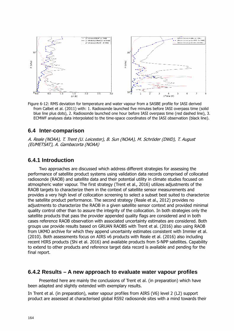
164

Figure 6-12: RMS deviation for temperature and water vapour from a SASBE profile for IASI derived

from Calbet et al. (2011) with: 1. Radiosonde launched five minutes before IASI overpass time (solid blue line plus dots), 2. Radiosonde launched one hour before IASI overpass time (red dashed line), 3. ECMWF analyses data interpolated to the time-space coordinates of the IASI observation (black line).

6.4 Inter-comparison

A. Reale (NOAA), T. Trent (U. Leicester), B. Sun (NOAA), M. Schröder (DWD), T. August (EUMETSAT), A. Gambacorta (NOAA)

6.4.1 Introduction

Two approaches are discussed which address different strategies for assessing the performance of satellite product systems using validation data records comprised of collocated radiosonde (RAOB) and satellite data and their potential utility in climate studies focused on atmospheric water vapour. The first strategy (Trent et al., 2016) utilizes adjustments of the RAOB targets to characterize them in the context of satellite sensor measurements and provides a very high level of collocation screening to select a subset best suited to characterize the satellite product performance. The second strategy (Reale et al., 2012) provides no adjustments to characterize the RAOB in a given satellite sensor context and provided minimal quality control other than to assure the integrity of the collocation. In both strategies only the satellite products that pass the provider appended quality flags are considered and in both cases reference RAOB observation with associated uncertainty estimates are considered. Both groups use provide results based on GRUAN RAOBS with Trent et al. (2016) also using RAOB from UKMO archive for which they append uncertainty estimates consistent with Immler et al. (2010). Both assessments focus on AIRS v6 products with Reale et al. (2016) also including recent HIRS products (Shi et al. 2016) and available products from S-NPP satellites. Capability to extend to other products and reference target data record is available and pending for the final report.

6.4.2 Results – A new approach to evaluate water va pour profiles

Presented here are mainly the conclusions of Trent et al. (in preparation) which have been adapted and slightly extended with exemplary results.

In Trent et al. (in preparation), water vapour profiles from AIRS (V6) level 2 (L2) support product are assessed at characterised global RS92 radiosonde sites with a mind towards their

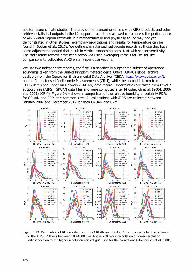
165

use for future climate studies. The provision of averaging kernels with AIRS products and other retrieval statistical outputs in the L2 support product has allowed us to access the performance of AIRS water vapour retrievals in a mathematically and physically sound way not yet demonstrated in other studies (exemplary applications and results for temperature can be found in Boylan et al., 2015). We define characterised radiosonde records as those that have some adjustment applied that result in vertical smoothing consistent with sensor sensitivity. The radiosonde records have been convolved using averaging kernels for like-for-like comparisons to collocated AIRS water vaper observations. We use two independent records, the first is a specifically augmented subset of operational soundings taken from the United Kingdom Meteorological Office (UKMO) global archive available from the Centre for Environmental Data Archival (CEDA, http://www.ceda.ac.uk/), named Characterised Radiosonde Measurements (CRM), while the second is taken from the GCOS Reference Upper-Air Network (GRUAN) data record. Uncertainties are taken from Level 2 support files (AIRS), GRUAN data files and were computed after Miloshevich et al. (2004, 2006 and 2009) (CRM). Figure 6-14 shows a comparison of the relative humidity uncertainty PDFs for GRUAN and CRM at 4 common sites. All collocations with AIRS are collected between January 2007 and December 2012 for both GRUAN and CRM.

Figure 6-13: Distribution of RH uncertainties from GRUAN and CRM at 4 common sites for levels closest to the AIRS L2 layers between 100-1000 hPa. Above 200 hPa interpolation of lower resolution radiosondes on to the higher resolution vertical grid used for the corrections (Miloshevich et al., 2004,

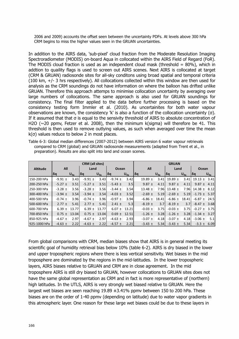
166

2006 and 2009) accounts the offset seen between the uncertainty PDFs. At levels above 300 hPa CRM begins to miss the higher values seen in the GRUAN uncertainties.

In addition to the AIRS data, 'sub-pixel' cloud fraction from the Moderate Resolution Imaging Spectroradiometer (MODIS) on-board Aqua in collocated within the AIRS Field of Regard (FoR). The MODIS cloud fraction is used as an independent cloud mask (threshold = 80%), which in addtion to quaility flags is used to screen out AIRS scenes. Next AIRS is collocated at target (CRM & GRUAN) radiosonde sites for all-sky conditons using broad spatial and temporal criteria (100 km, +/- 3 hrs respectively). All collocations collected within this window are then used for analysis as the CRM soundings do not have information on where the balloon has drifted unlike GRUAN. Therefore this approach attemps to minimise collocation uncertainty by averaging over large numbers of collocations. The same approach is also used for GRUAN soundings for consistency. The final filter applied to the data before further processing is based on the consistency testing form Immler et al. (2010). As uncertainites for both water vapour observations are known, the consistency 'k' is also a function of the collocation uncertainty (σ). If it assumed that that σ is equal to the sensivity threshold of AIRS to absolute concentration of H2O (~20 ppmv, Fetzer et al. 2008), then the minimum k(sigma) will therefore be 41. This threshold is then used to remove outlying values, as such when averaged over time the mean k(σ) values reduce to below 2 in most places.

Table 6-3: Global median differences (2007-2012) between AIRS version 6 water vapour retrievals compared to CRM (global) and GRUAN radiosonde measurements (adapted from Trent et al., in preparation). Results are also split into land and ocean scenes.

δq δq δq δq δq δq

150-200 hPa -9.91 ± 3.43 -9.91 ± 3.43 -9.74 ± 3.42 19.89 ± 3.41 19.89 ± 3.41 19.13 ± 3.41

200-250 hPa -5.27 ± 3.51 -5.27 ± 3.51 -5.43 ± 3.5 9.87 ± 4.11 9.87 ± 4.11 9.87 ± 4.11

250-300 hPa -3.28 ± 3.56 -3.28 ± 3.56 -3.44 ± 3.54 13.48 ± 7.96 13.48 ± 7.96 14.38 ± 8.12

300-400 hPa -3.94 ± 3.54 -3.94 ± 3.54 -4.03 ± 3.52 -2.69 ± 5.19 -2.69 ± 5.19 -1.73 ± 5.37

400-500 hPa -0.74 ± 3.96 -0.74 ± 3.96 -0.97 ± 3.94 -6.86 ± 18.41 -6.86 ± 18.41 -6.87 ± 24.5

500-600 hPa 2.77 ± 5.41 2.77 ± 5.41 2.41 ± 5.3 -8.19 ± 3.7 -8.19 ± 3.7 -8.47 ± 3.68

600-700 hPa 6.39 ± 13.77 6.39 ± 13.77 6.07 ± 13.21 -0.03 ± 3.75 -0.03 ± 3.75 -0.27 ± 3.75

700-850 hPa 0.75 ± 13.04 0.75 ± 13.04 0.69 ± 12.51 -1.26 ± 3.28 -1.26 ± 3.28 -1.34 ± 3.27

850-925 hPa -4.67 ± 2.97 -4.67 ± 2.97 -4.63 ± 2.93 -3.07 ± 4.18 -3.07 ± 4.18 -3.06 ± 5.1

925-1000 hPa -4.63 ± 2.22 -4.63 ± 2.22 -4.57 ± 2.21 -3.43 ± 5.34 -3.43 ± 5.34 -3.3 ± 6.09

CRM (all sites) GRUAN

Altitude All Land Ocean

Uδq Uδq Uδq Uδq Uδq Uδq

All Land Ocean

From global comparisons with CRM, median biases show that AIRS is in general meeting its scientific goal of humidity retrieval bias below 10% (table 6-2). AIRS is dry biased in the lower and upper tropospheric regions where there is less vertical sensitivity. Wet biases in the mid troposphere are dominated by the regions in the mid-latitudes. In the lower tropospheric layers, AIRS biases relative to GRUAN and CRM are in close agreement. In the mid troposphere AIRS is still dry biased to GRUAN, however collocations to GRUAN sites does not have the same global representation as CRM and in fact is more representative of (northern) high latitudes. In the UTLS, AIRS is very strongly wet biased relative to GRUAN. Here the largest wet biases are seen reaching 19.89 ±3.41% ppmv between 150 to 200 hPa. These biases are on the order of 1-40 ppmv (depending on latitude) due to water vapor gradients in this atmospheric layer. One reason for these large wet biases could be due to these layers in

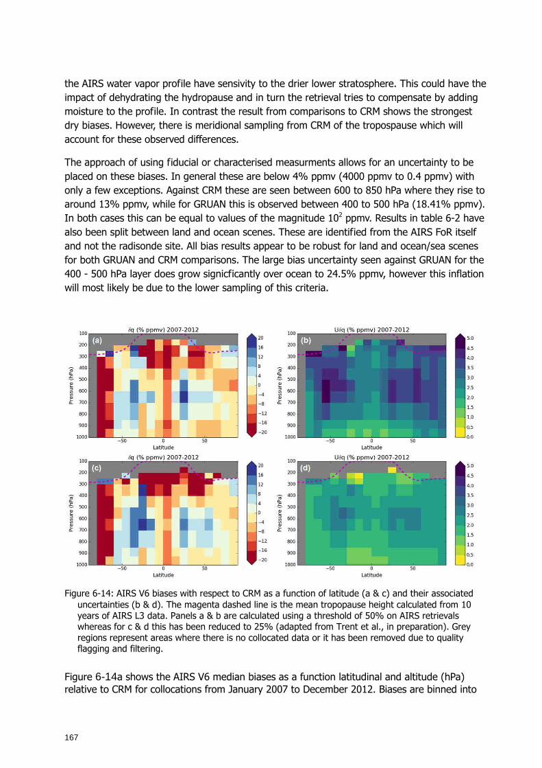
167

the AIRS water vapor profile have sensivity to the drier lower stratosphere. This could have the impact of dehydrating the hydropause and in turn the retrieval tries to compensate by adding moisture to the profile. In contrast the result from comparisons to CRM shows the strongest dry biases. However, there is meridional sampling from CRM of the tropospause which will account for these observed differences.

The approach of using fiducial or characterised measurments allows for an uncertainty to be placed on these biases. In general these are below 4% ppmv (4000 ppmv to 0.4 ppmv) with only a few exceptions. Against CRM these are seen between 600 to 850 hPa where they rise to around 13% ppmv, while for GRUAN this is observed between 400 to 500 hPa (18.41% ppmv). In both cases this can be equal to values of the magnitude 102 ppmv. Results in table 6-2 have also been split between land and ocean scenes. These are identified from the AIRS FoR itself and not the radisonde site. All bias results appear to be robust for land and ocean/sea scenes for both GRUAN and CRM comparisons. The large bias uncertainty seen against GRUAN for the 400 - 500 hPa layer does grow signicficantly over ocean to 24.5% ppmv, however this inflation will most likely be due to the lower sampling of this criteria.

Figure 6-14: AIRS V6 biases with respect to CRM as a function of latitude (a & c) and their associated

uncertainties (b & d). The magenta dashed line is the mean tropopause height calculated from 10 years of AIRS L3 data. Panels a & b are calculated using a threshold of 50% on AIRS retrievals whereas for c & d this has been reduced to 25% (adapted from Trent et al., in preparation). Grey regions represent areas where there is no collocated data or it has been removed due to quality flagging and filtering.

Figure 6-14a shows the AIRS V6 median biases as a function latitudinal and altitude (hPa) relative to CRM for collocations from January 2007 to December 2012. Biases are binned into

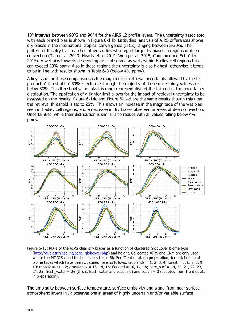
168

10° intervals between 90°S and 90°N for the AIRS L2 profile layers. The uncertainty associated with each binned bias is shown in Figure 6-14b. Latitudinal analysis of AIRS differences shows dry biases in the international tropical convergence (ITCZ) ranging between 5-30%. The pattern of this dry bias matches other studies who report large dry biases in regions of deep convection (Tian et al. 2013; Hearty et al. 2014; Wong et al. 2015; Courcoux and Schröder 2015). A wet bias towards descending air is observed as well, within Hadley cell regions this can exceed 20% ppmv. Also in these regions the uncertainty is also highest, otherwise it tends to be in line with results shown in Table 6-3 (below 4% ppmv).

A key issue for these comparisons is the magnitude of retrieval uncertainty allowed by the L2 product. A threshold of 50% is extreme, though the majority of these uncertainty values are below 50%. This threshold value infact is more representative of the tail end of the uncertainty distribution. The application of a tighter limit allows for the impact of retrieval uncertainty to be assessed on the results. Figure 6-14c and Figure 6-14d are the same results though this time the retrieval threshold is set to 25%. This shows an increase in the magnitude of the wet bias seen in Hadley cell regions, and a decrease in dry biases observed in areas of deep convection. Uncertainties, while their distribution is similar also reduce with all values falling below 4% ppmv.

Figure 6-15: PDFs of the AIRS clear sky biases as a function of clustered GlobCover biome type (http://due.esrin.esa.int/page_globcover.php) and height. Collocated AIRS and CRM are only used where the MODIS cloud fraction is less than 1%. See Trent et al. (in preparation) for a definition of biome types which have been clustered here as follows: croplands = 1, 2, 3, 4; forest = 5, 6, 7, 8, 9, 10; mosaic = 11, 12; grasslands = 13, 14, 15; flooded = 16, 17, 18; bare_surf = 19, 20, 21, 22, 23, 24, 25; fresh_water = 26 (this is fresh water and coastline) and ocean = 0 (adapted from Trent et al., in preparation).

The ambiguity between surface temperature, surface emissivity and signal from near surface atmospheric layers in IR observations in areas of highly uncertain and/or variable surface

169

characteristics is challenging if near surface temperature and humidity are retrieved. E.g., the results from Courcoux and Schröder (2016) suggest maximum biases between ATOVS and AIRS over tropical land surfaces are linked to areas of rain forest. Thus, the need for accurate surface characterisation for the IR based water vapour CDR was analysed.

Figure 6-15 characterises the AIRS clear-sky bias relative to CRM for different surface/biome types. In the surface layer, areas prone to regular flooding tend to be wetter biased compared to fresh water/coastal and ocean cases while vegetated and bare surefaces show similar performace. In the next surface layer (850-925 hPa) bare surfaces show slight modal wet biases in contradiction to the other biome types that are consistent with the global dry bias (Table 6-3). This is further exaggerated in the third lowest tropospheric layer where the modal bare surface clear-sky bias is closer to 10% wet biased. Here there is also a sepration of other biome types. Flooded and fresh water surfaces are stil dry biased while mosaic and ocean surfaces are close to 0% while grassland, forest and croplands are wet biased by around 5% ppmv.

Strong changes in surface emissivity on short time scales are very difficult to capture by microwave retrievals, used here for first guess retrieval. Also, the perceived colder surface could affect the retrieved atmospheric temperature. In any respect these results point to a need for accurate surface characterisation (emissivity and skin temperature) for all observed wavelengths in order to overcome the ambiguity in IR based near surface retrievals. This is particularly relevant for remote areas such as tropical rain forests in which the current ground-based and in-situ networks hardly provide reference data, further supporting the recommendation to GRUAN on the network enhancement (Bodecker et al. 2014, see also section 6). Besides a potential enhancement of reference networks this gap should be filled with satellite data of improved quality.

Among others, the emerging AIRS climate data record provides specific humidity in the upper troposphere and thus data which is of utmost relevance to analyse the water vapour feedback. Analysis of AIRS biases as a function of latitude using CRM reveals sensitivity to large motion of water vapour, especially in the ITCZ. In this region AIRS is dry biased by over 20% ppmv to the ascending air mass at the equator and wet biased to the descending air mass around the Hadley cells (Trent et al., in preparation). Understanding these biases over climate time scales is vital for studies into water vapour feedback. In particular the largest contribution to the water vapour feedback stems from the tropical free troposphere, and the outgoing longwave radiation is highly sensitive to changes at the dry end of the humidity distribution as e.g. in regions of descending air masses around the Hadley cells.

An important pre-requisite for such an effort is the availability of high quality reference data with uncertainty information. Here we have reprocessed global radiosonde data for the period January 2007 – December 2012 and demonstrated feasibility for a reprocessing of RS92 radiosonde archives. We also demonstrate the benefits of characterised measurements from newtorks like GRUAN over the operational records, through the bias uncertainty estimates. A stable and bias corrected multi-station radiosonde archive is of high value for the validation of satellite-based water vapour products. Therefore, reducing these uncertainties is key for the assessment of any climate record; with the production of a stable, characterised, global, retroactive radiosonde archive a real challenge. Further development and reprocessing of radiosonde data is needed to allow for satellite records spanning from the present back to the late 1970s to be exploited for climate analysis.

The value of systematic differences can be enhanced if the total difference can be broken down into individual components. In the characterisation of the RS92 archive we also compare the vertical distribution of CRM uncertainty with those from GRUAN. One apparent difference is the inability of CRM to fully capture the random uncertainty component which could allow for

170

collocated profiles that should be excluded during the consistency test. A large variety of such structural uncertainties can contribute to the total bias (see Kummerow et al. 2011 for a brief discussion). Here we discuss structural uncertainties associated with subpixel variability, clear sky sampling and cloud fraction as well as surface characteristics.

The AIRS water vapour data is an example of data which is based on the combination of hyperspectral and microwave observations. Similar retrievals exist for IASI and CrIS, though they have not been reprocessed consistently until now. With EUMETSAT EPS-SG at least the IASI observations will be sustained until beyond 2030. Thus, we may speak of a high potential for climate monitoring using hyperspectral data in a forward looking sense.

6.4.3 Results - Inter-comparisons using NPROVS+

The NOAA Products Validation System (NPROVS) (Reale et al. 2012) was established at NOAA NESDIS Center for Satellite Applications and Research (STAR) in 2008 to provide a centralized capability for compiling collocations of conventional radiosonde, numerical weather prediction (NWP) analysis and atmospheric temperature and water vapour sounding profiles derived from different satellites (i.e., NOAA, EUMETSAT, NASA-EOS)), sensors suites (HIRS, IASI, AIRS) and associated derived product suites. The primary objective of NPROVS is to support NOAA Joint Polar Satellite System (JPSS) calibration/validation (cal/val) programs for atmospheric soundings from the Suomi National Polar-orbiting Partnership (S-NPP). The capability to routinely inter-compare satellite sounding products against radiosonde and NWP products using NPROVS collocation data records has been highly useful for assessing sounding performance over a variety of seasonal and regional weather conditions and targeting problem areas for algorithm improvement. However, challenges are present for NPROVS to conduct robust assessment of satellite products in terms of absolute accuracy given the accuracy issues in conventional RAOBs (see Sun et al. 2010, and 2013). Thus, in 2013 the NPROVS was expanded to create collocations with available reference radiosonde observations from the GCOS Reference Upper Air Network (GRUAN, Seidel et al. 2009) which include traceable observations and uncertainty estimates (Immler et al. 2010), referred to as NPROVS+. These were later augmented by sets of NOAA Joint Polar Satellite System (JPSS) funded dedicated radiosonde synchronized with S-NPP overpass and launched at United States Department of Energy (DOE) Atmospheric Radiation Measurement (ARM) sites (Tobin et al. 2006) and also in conjunction with selected data intensive research programs targeting the tropical oceans.

The assessments reported in this section are based on global collocations of GRUAN radiosonde and satellite water vapour profiles compiled by NPROVS+ for the time period January 2013 through November 2014 shown in Figure 6-17. This corresponds to the available period of record for the HIRS based water vapour mixing ratio (MR, g/kg) profiles from MetOp-A from the National Centers for Environmental Information (NCEI) (Shi et al. 2016) that were specially integrated into NPROVS+ for this report. Other moisture profiles assessed are the NOAA Unique Combined Atmospheric Processing System (NUCAPS) from Metop-A (Gambacorta et al. 2012), the AIRS version 5 (v5) from Aqua-EOS (Susskind et al. 2011) and the ECMWF Analysis. The satellite profiles used are constrained to the subsets of acceptable infrared (IR) based profiles as designated by the respective providers. Since the HIRS profiles are at the lowest vertical density, namely 7-levels from 1000 to 300 hPa, all profiles are interpolated (log-linear) to these levels for comparison.

The advantage of using GRUAN data is that the radiosonde observations are calibrated through an unbroken traceability chain to SI or community standards with the uncertainty interval in each step in the chain fully characterized, meaning the resulting estimates can be used with high confidence that the true measurement is within the uncertainty (Immler et al. 2010). A

171

current disadvantage is that the global distribution of GRUAN sites providing radiosonde data is limited. Furthermore, there are relatively few synchronized GRUAN radiosonde and respective satellites observations although guidance to account for mismatch error is available (Sun et al. 2010). Subsets of JPSS funded GRUAN processed radiosondes synchronized with S-NPP (mid-afternoon orbit) are available which offers targeted observations for AIRS comparisons.

This leads to the question of what spatial and temporal windows to use for the results of this section. NPROVS (or NPROVS+) compiles the single, closest collocation for a given satellite within +/- 6 hr and 150 km. This nominally insures at least one collocation from any given satellite for a given radiosonde, optimizes the global distribution and also facilitates studies on the impact of mismatch on performance (also see section 6.3).

Figure 6-16 summarizes a preliminary analysis on the impact of the mismatch window on a global assessment and was done using collocated GRUAN radiosonde and the HIRS, MetOp-A, MR profiles from the sites shown in Figure 6-16. The HIRS NCEI profiles include cloudiness designations which denote mostly clear (probability of cloud less than 10%), partly cloudy (probability of clouds from 10% to 75%) and cloudy (probability of cloud greater 75%) scenes; only clear and partly cloudy designations were included. The top set of plots in figure Figure 6-16 show RMS differences for HIRS-minus-GRUAN in units of MR fractional difference (%) defined as

Eq. 6.2

The left-side plots are for collocations within +/- 3 hour and the right-side plots are for collocations outside of +/- 3 hours. As can be seen, the RMS differences show about a 10% reduction in RMS differences for the samples within 3 hours mainly between 700 and 400 hPa. At 500 hPa, multiplying the respective RMS and mean MR (along the inside x-axis) yields an RMS reduction from 0.367 to 0.295 g/kg using samples within +/- 3 hr samples compared to outside +/- 3 hr.

The lower plots of Figure 6-16 show results for the same samples but using “k” profiles based on the GRUAN uncertainty as described below.

The GRUAN consistency equation expanded from Immler et al. (2010) is

Eq. 6.3

where m1 and m2 denote the comparative measurements from different platforms, for example, satellite derived vs GRUAN radiosonde MR profiles, and u1 and u2 are the respective uncertainty estimates. Sigma ( denotes additional uncertainty due to uncertainties arising from representativeness.

GRUAN reports moisture uncertainty in terms of relative humidity (RH). Since satellite sensors directly measure water vapour molecules or mixing ratio, RH uncertainty is converted MR uncertainty by

Eq. 6.4

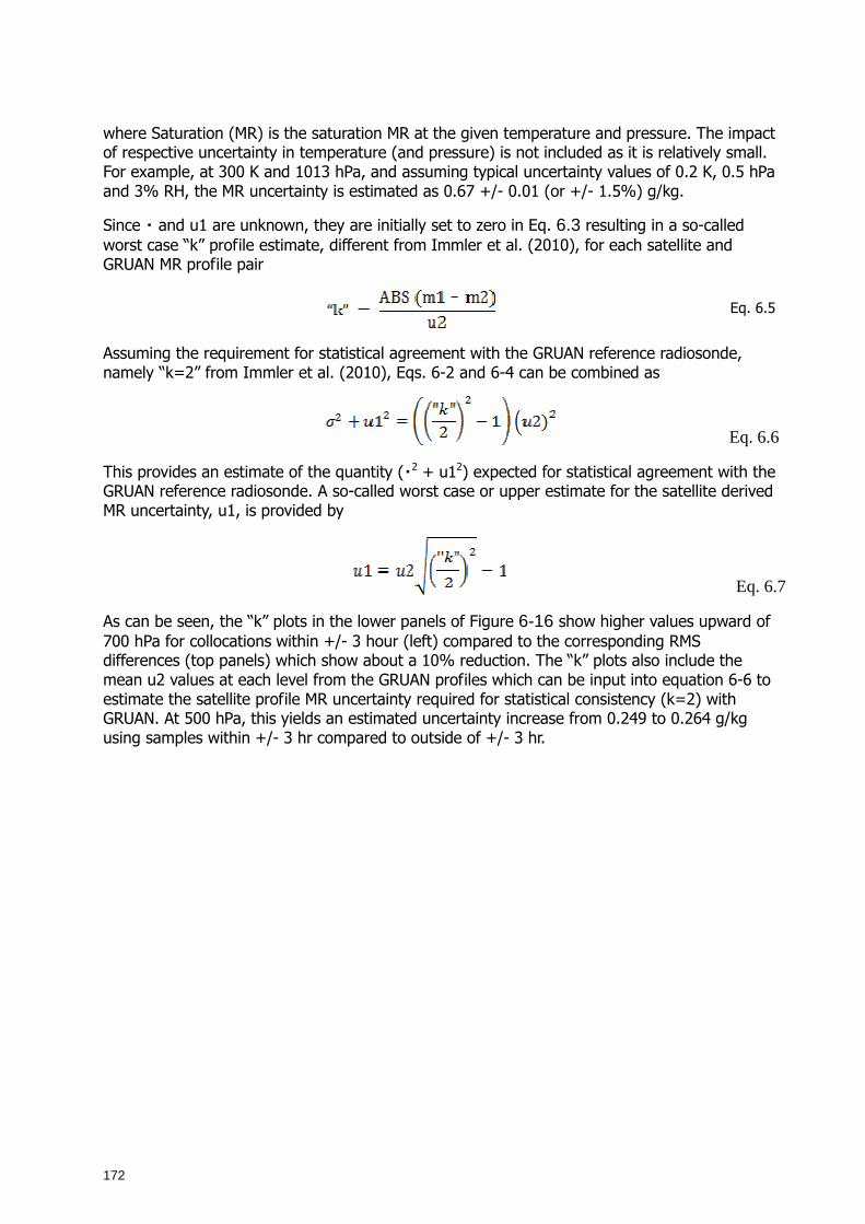
172

where Saturation (MR) is the saturation MR at the given temperature and pressure. The impact of respective uncertainty in temperature (and pressure) is not included as it is relatively small. For example, at 300 K and 1013 hPa, and assuming typical uncertainty values of 0.2 K, 0.5 hPa and 3% RH, the MR uncertainty is estimated as 0.67 +/- 0.01 (or +/- 1.5%) g/kg.

Since and u1 are unknown, they are initially set to zero in Eq. 6.3 resulting in a so-called worst case “k” profile estimate, different from Immler et al. (2010), for each satellite and GRUAN MR profile pair

Eq. 6.5

Assuming the requirement for statistical agreement with the GRUAN reference radiosonde, namely “k=2” from Immler et al. (2010), Eqs. 6-2 and 6-4 can be combined as

Eq. 6.6

This provides an estimate of the quantity (2 + u12) expected for statistical agreement with the GRUAN reference radiosonde. A so-called worst case or upper estimate for the satellite derived MR uncertainty, u1, is provided by

Eq. 6.7

As can be seen, the “k” plots in the lower panels of Figure 6-16 show higher values upward of 700 hPa for collocations within +/- 3 hour (left) compared to the corresponding RMS differences (top panels) which show about a 10% reduction. The “k” plots also include the mean u2 values at each level from the GRUAN profiles which can be input into equation 6-6 to estimate the satellite profile MR uncertainty required for statistical consistency (k=2) with GRUAN. At 500 hPa, this yields an estimated uncertainty increase from 0.249 to 0.264 g/kg using samples within +/- 3 hr compared to outside of +/- 3 hr.

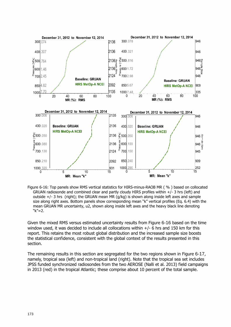
173

Figure 6-16: Top panels show RMS vertical statistics for HIRS-minus-RAOB MR ( % ) based on collocated GRUAN radiosonde and combined clear and partly cloudy HIRS profiles within +/- 3 hrs (left) and outside +/- 3 hrs (right); the GRUAN mean MR (g/kg) is shown along inside left axes and sample size along right axes. Bottom panels show corresponding mean “k” vertical profiles (Eq. 6.4) with the mean GRUAN MR uncertainty, u2, shown along inside left axes and the heavy black line denoting “k”=2.

Given the mixed RMS versus estimated uncertainty results from Figure 6-16 based on the time window used, it was decided to include all collocations within +/- 6 hrs and 150 km for this report. This retains the most robust global distribution and the increased sample size boosts the statistical confidence, consistent with the global context of the results presented in this section. The remaining results in this section are segregated for the two regions shown in Figure 6-17, namely, tropical sea (left) and non-tropical land (right). Note that the tropical sea set includes JPSS funded synchronized radiosondes from the two AEROSE (Nalli et al. 2013) field campaigns in 2013 (red) in the tropical Atlantic; these comprise about 10 percent of the total sample.

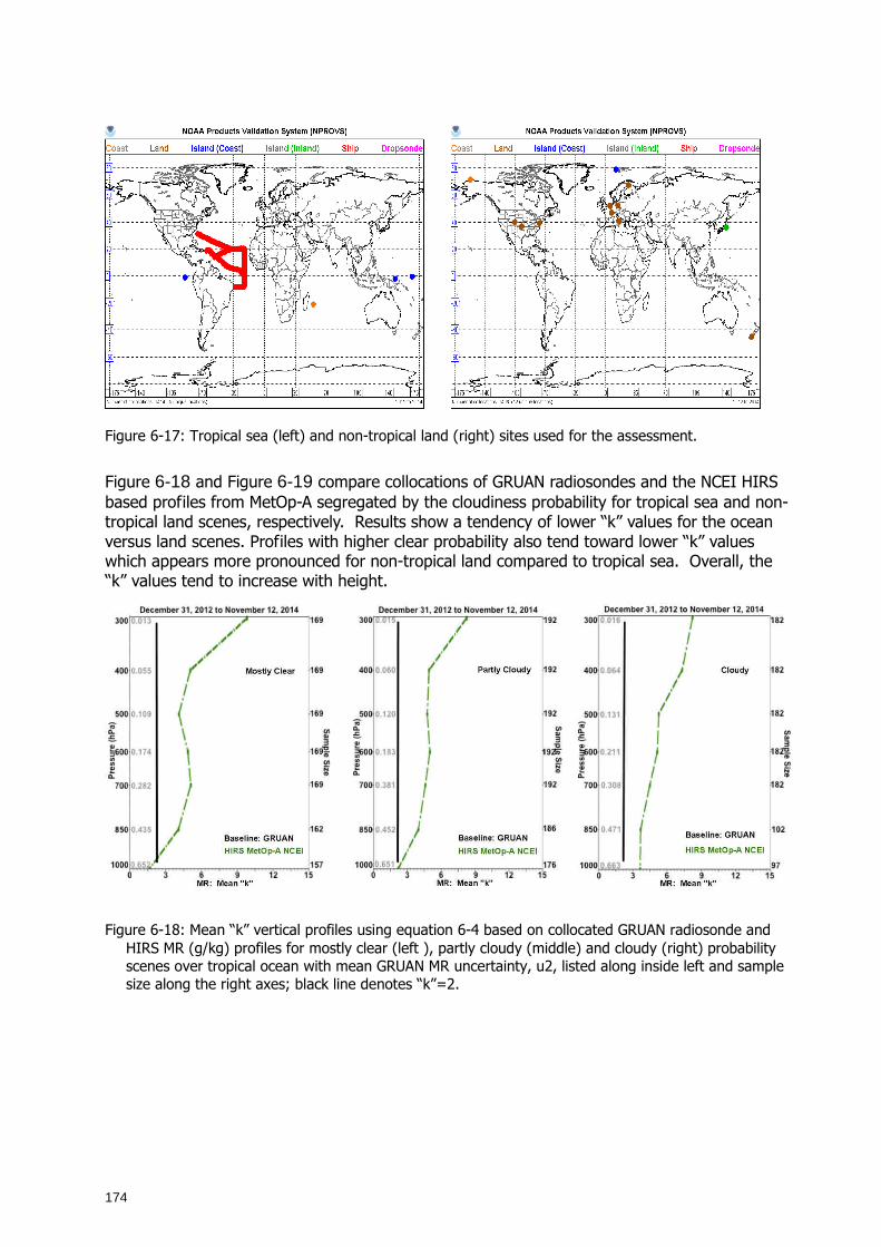
174

Figure 6-17: Tropical sea (left) and non-tropical land (right) sites used for the assessment.

Figure 6-18 and Figure 6-19 compare collocations of GRUAN radiosondes and the NCEI HIRS based profiles from MetOp-A segregated by the cloudiness probability for tropical sea and non-tropical land scenes, respectively. Results show a tendency of lower “k” values for the ocean versus land scenes. Profiles with higher clear probability also tend toward lower “k” values which appears more pronounced for non-tropical land compared to tropical sea. Overall, the “k” values tend to increase with height.

Figure 6-18: Mean “k” vertical profiles using equation 6-4 based on collocated GRUAN radiosonde and HIRS MR (g/kg) profiles for mostly clear (left ), partly cloudy (middle) and cloudy (right) probability scenes over tropical ocean with mean GRUAN MR uncertainty, u2, listed along inside left and sample size along the right axes; black line denotes “k”=2.

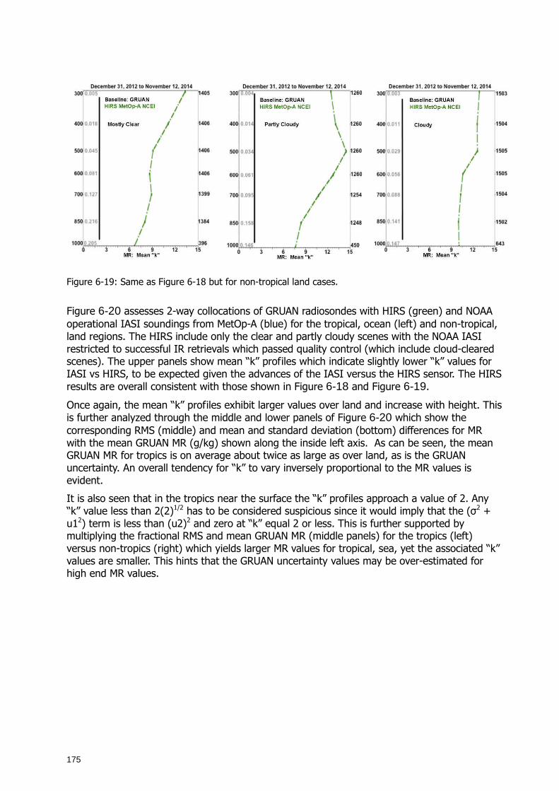
175

Figure 6-19: Same as Figure 6-18 but for non-tropical land cases.

Figure 6-20 assesses 2-way collocations of GRUAN radiosondes with HIRS (green) and NOAA operational IASI soundings from MetOp-A (blue) for the tropical, ocean (left) and non-tropical, land regions. The HIRS include only the clear and partly cloudy scenes with the NOAA IASI restricted to successful IR retrievals which passed quality control (which include cloud-cleared scenes). The upper panels show mean “k” profiles which indicate slightly lower “k” values for IASI vs HIRS, to be expected given the advances of the IASI versus the HIRS sensor. The HIRS results are overall consistent with those shown in Figure 6-18 and Figure 6-19.

Once again, the mean “k” profiles exhibit larger values over land and increase with height. This is further analyzed through the middle and lower panels of Figure 6-20 which show the corresponding RMS (middle) and mean and standard deviation (bottom) differences for MR with the mean GRUAN MR (g/kg) shown along the inside left axis. As can be seen, the mean GRUAN MR for tropics is on average about twice as large as over land, as is the GRUAN uncertainty. An overall tendency for “k” to vary inversely proportional to the MR values is evident.

It is also seen that in the tropics near the surface the “k” profiles approach a value of 2. Any “k” value less than 2(2)1/2 has to be considered suspicious since it would imply that the (σ2 + u12) term is less than (u2)2 and zero at “k” equal 2 or less. This is further supported by multiplying the fractional RMS and mean GRUAN MR (middle panels) for the tropics (left) versus non-tropics (right) which yields larger MR values for tropical, sea, yet the associated “k” values are smaller. This hints that the GRUAN uncertainty values may be over-estimated for high end MR values.

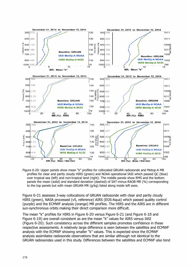
176

Figure 6-20: Upper panels show mean “k” profiles for collocated GRUAN radiosonde and Metop-A MR

profiles for clear and partly cloudy HIRS (green) and NOAA operational IASI which passed QC (blue) over tropical sea (left) and non-tropical land (right). The middle panels show RMS and the bottom panels the mean (solid) and standard deviation (dashed) of SAT-minus-RAOB MR (%) corresponding to the top panels but with mean GRUAN MR (g/kg) listed along inside left axes.

Figure 6-21 assesses 3-way collocations of GRUAN radiosonde with clear and partly cloudy HIRS (green), NASA processed (v5, reference) AIRS (EOS-Aqua) which passed quality control (purple) and the ECMWF analysis (orange) MR profiles. The HIRS and the AIRS are in different sun-synchronous orbits making their direct comparison more difficult.

The mean “k” profiles for HIRS in Figure 6-20 versus Figure 6-21 (and Figure 6-18 and Figure 6-19) are overall consistent as are the mean “k” values for AIRS versus IASI (Figure 6-20). Such consistency across the different samples promotes confidence in these respective assessments. A relatively large difference is seen between the satellites and ECMWF analysis with the ECMWF showing smaller “k” values. This is expected since the ECMWF analysis assimilates radiosonde observations that are similar although not identical to the GRUAN radiosondes used in this study. Differences between the satellites and ECMWF also tend

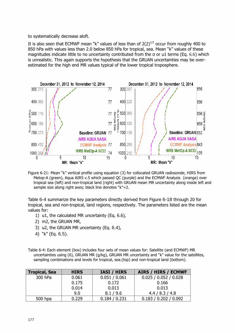
177

to systematically decrease aloft.

It is also seen that ECMWF mean “k” values of less than of 2(2)1/2 occur from roughly 400 to 850 hPa with values less than 2.0 below 850 hPa for tropical, sea. Mean “k” values of these magnitudes indicate little to no uncertainty contributed from the σ or u1 terms (Eq. 6.6) which is unrealistic. This again supports the hypothesis that the GRUAN uncertainties may be over-estimated for the high end MR values typical of the lower tropical troposphere.

Figure 6-21: Mean “k” vertical profile using equation (3) for collocated GRUAN radiosonde, HIRS from

Metop-A (green), Aqua AIRS v.5 which passed QC (purple) and the ECMWF Analysis (orange) over tropical sea (left) and non-tropical land (right) with GRUAN mean MR uncertainty along inside left and sample size along right axes; black line denotes “k”=2.

Table 6-4 summarize the key parameters directly derived from Figure 6-18 through 20 for tropical, sea and non-tropical, land regions, respectively. The parameters listed are the mean values for:

1) u1, the calculated MR uncertainty (Eq. 6.6), 2) m2, the GRUAN MR,

3) u2, the GRUAN MR uncertainty (Eq. 6.4),

4) “k” (Eq. 6.5).

Table 6-4: Each element (box) includes four sets of mean values for: Satellite (and ECMWF) MR uncertainties using (6), GRUAN MR (g/kg), GRUAN MR uncertainty and “k” value for the satellites, sampling combinations and levels for tropical, sea.(top) and non-tropical land (bottom).

Tropical, Sea HIRS IASI / HIRS AIRS / HIRS / ECMWF

300 hPa 0.061 0.175 0.014 9.0

0.051 / 0.061 0.172 0.013

8.1 / 9.6

0.025 / 0.052 / 0.028 0.166 0.013

4.4 / 8.3 / 4.8 500 hpa 0.229 0.184 / 0.231 0.183 / 0.202 / 0.092

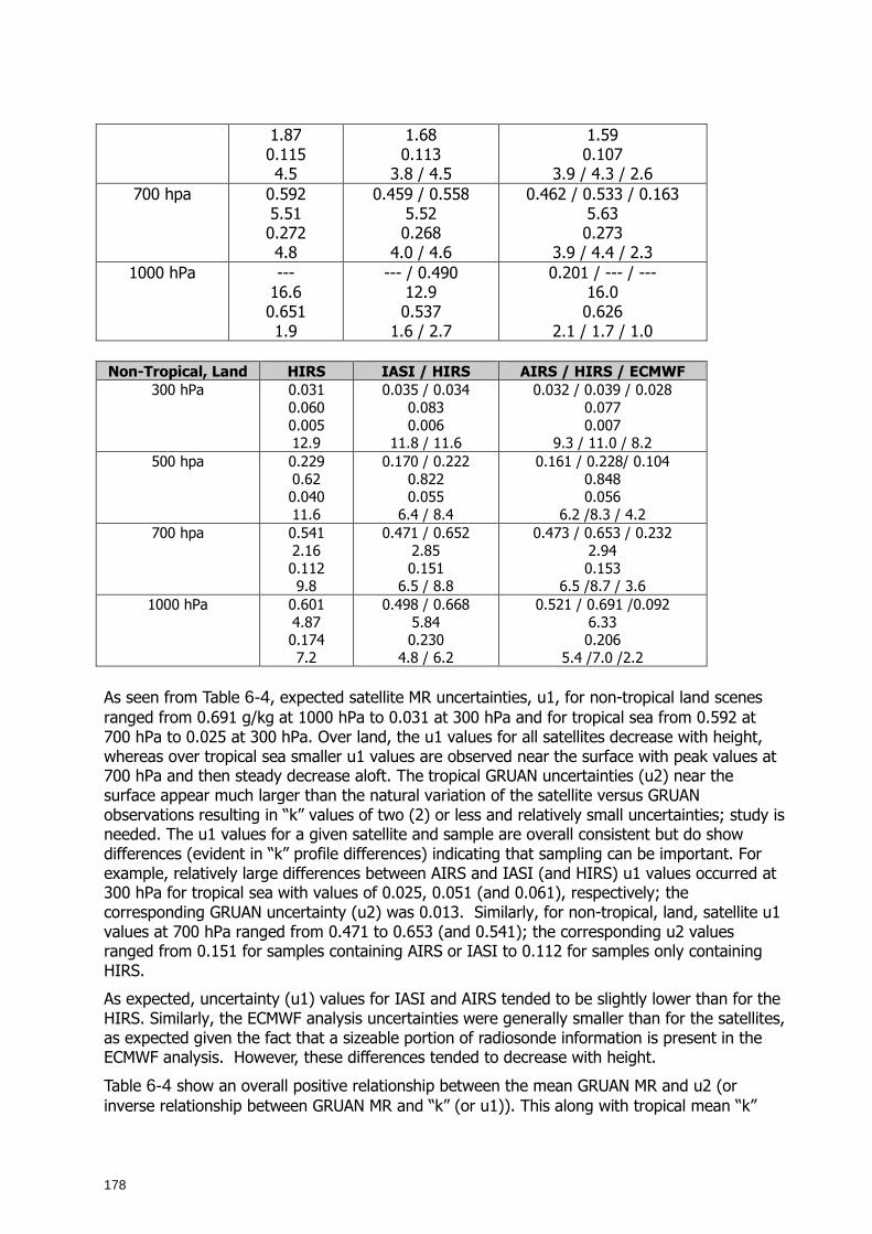
178

1.87 0.115 4.5

1.68 0.113

3.8 / 4.5

1.59 0.107

3.9 / 4.3 / 2.6 700 hpa 0.592

5.51 0.272 4.8

0.459 / 0.558 5.52 0.268

4.0 / 4.6

0.462 / 0.533 / 0.163 5.63 0.273

3.9 / 4.4 / 2.3 1000 hPa ---

16.6 0.651 1.9

--- / 0.490 12.9 0.537

1.6 / 2.7

0.201 / --- / --- 16.0 0.626

2.1 / 1.7 / 1.0 Non-Tropical, Land HIRS IASI / HIRS AIRS / HIRS / ECMWF

300 hPa 0.031 0.060 0.005 12.9

0.035 / 0.034 0.083 0.006

11.8 / 11.6

0.032 / 0.039 / 0.028 0.077 0.007

9.3 / 11.0 / 8.2 500 hpa 0.229

0.62 0.040 11.6

0.170 / 0.222 0.822 0.055

6.4 / 8.4

0.161 / 0.228/ 0.104 0.848 0.056

6.2 /8.3 / 4.2 700 hpa 0.541

2.16 0.112 9.8

0.471 / 0.652 2.85 0.151

6.5 / 8.8

0.473 / 0.653 / 0.232 2.94 0.153

6.5 /8.7 / 3.6 1000 hPa 0.601

4.87 0.174 7.2

0.498 / 0.668 5.84 0.230

4.8 / 6.2

0.521 / 0.691 /0.092 6.33 0.206

5.4 /7.0 /2.2 As seen from Table 6-4, expected satellite MR uncertainties, u1, for non-tropical land scenes ranged from 0.691 g/kg at 1000 hPa to 0.031 at 300 hPa and for tropical sea from 0.592 at 700 hPa to 0.025 at 300 hPa. Over land, the u1 values for all satellites decrease with height, whereas over tropical sea smaller u1 values are observed near the surface with peak values at 700 hPa and then steady decrease aloft. The tropical GRUAN uncertainties (u2) near the surface appear much larger than the natural variation of the satellite versus GRUAN observations resulting in “k” values of two (2) or less and relatively small uncertainties; study is needed. The u1 values for a given satellite and sample are overall consistent but do show differences (evident in “k” profile differences) indicating that sampling can be important. For example, relatively large differences between AIRS and IASI (and HIRS) u1 values occurred at 300 hPa for tropical sea with values of 0.025, 0.051 (and 0.061), respectively; the corresponding GRUAN uncertainty (u2) was 0.013. Similarly, for non-tropical, land, satellite u1 values at 700 hPa ranged from 0.471 to 0.653 (and 0.541); the corresponding u2 values ranged from 0.151 for samples containing AIRS or IASI to 0.112 for samples only containing HIRS.

As expected, uncertainty (u1) values for IASI and AIRS tended to be slightly lower than for the HIRS. Similarly, the ECMWF analysis uncertainties were generally smaller than for the satellites, as expected given the fact that a sizeable portion of radiosonde information is present in the ECMWF analysis. However, these differences tended to decrease with height.

Table 6-4 show an overall positive relationship between the mean GRUAN MR and u2 (or inverse relationship between GRUAN MR and “k” (or u1)). This along with tropical mean “k”

179

values approaching 2 or less suggests that the GRUAN uncertainties may be overestimated at the high end of the MR range.

In summary, the above results demonstrate how the sets of collocated observations can be used to estimate satellite (and ECMWF) profile uncertainties traceable to the GRUAN radiosondes. In addition, these observations can provide a mechanism for feedback to GRUAN.

6.4.4 Summary

Results are presented using NPROVS+ which routinely collocates GRUAN radiosondes with multiple satellite product suites; GRUAN radiosondes include traceable uncertainty estimates. These collocations are used to calculate mean “k” profiles leading to uncertainty estimates for the satellite based MR (g/kg) profiles. These are provided for IR based retrievals from HIRS and IASI onboard MetOp-A and AIRS onboard Aqua-EOS. The period of record is an approximately 2 years from January 2013 to November 2014 (so any inference on long-term performance and climate scale is minimal). The “k” profiles are a measure of the natural variability of the satellite-minus-radiosonde variations scaled by the GRUAN uncertainty. Results were compiled at 7 pressure levels from 1000 hPa to 300 hPa as defined for the HIRS NCEI product suite from MetOp-A, requiring interpolation of the higher vertical density GRUAN radiosonde, other satellites and ECMWF analysis compared in this section.

We summarize:

• HIRS show slightly higher MR uncertainties than for AIRS and IASI which are overall similar • Satellite product uncertainty values over non-tropical land range from 0.668 g/kg at 1000

hPa to 0.031 g/kg at 300 hPa; associated GRUAN uncertainty estimates range from 0.174 to 0.005 g/kg.

• Satellite product uncertainty values over tropical sea for satellites range from 0.592 g/kg at 700 hPa to 0.025g/kg at 300 hPa; associated GRUAN uncertainty estimates range from 0.273 to 0.014 g/kg.

• ECMWF uncertainties were generally lower than for satellites (as expected) but differences decreased with height

Possible overestimations of GRUAN uncertainties (u2) for high-end MR values may be evident.

The results presented in this section indicate that MR profiles for the 3 suites of satellite products performed better over tropical sea versus non-tropical land for probable clear vs cloudy scenes.

Overall performance of the hyper-spectral products from IASI onboard MetOp-A and AIRS Aqua-EOS appeared slightly better (lower uncertainty) than those from HIRS consistent with sensor advancements. In general, u1 values were positively correlated to the mean MR value for the sample, level. A possible misleading factor in this interpretation is that the GRUAN uncertainties at the high end of the observed MR range may be overestimated. Similarly, performance appears to decrease with height particularly above 400 hPa. This is more likely due to decreased satellite sensitivity at low end of MR values (less than 0.100 g/kg).

Overall, the satellite products provide consistent and reliable global representation of atmospheric water vapour water.

180

7 Conclusions The executive summary (section 1) contains major conclusions and recommendations

and an overview of available output is given in section 2.1. Here we provide short answers to the G-VAP science and technical questions (see section 2.3):

• Q1a-c): How large are the differences in observed temporal changes in long-term satellite data records of water vapour on global and regional scales?

Are the observed temporal changes and anomalies, on global and regional scale, in line with theoretical expectations?

Are the differences in observed temporal changes within uncertainty limits?

Trends in TCWV are typically significantly different among long-term data records over the (tropical) ocean, exhibit a fairly large spread and are typically outside theoretical expectation. The main exceptions are differences between data records based on SSM/I only and ERA-20C. Also distinct regions of maxima in absolute differences among trend estimates are evident over tropical South America, Central Africa and Sahara (section 4.3.1).

Profiles of trend estimates, based on regional averages over the tropics and the northern and southern hemispheres, are to a large extent significantly different. Differences are smallest near the surface and the spread is larger over the southern than over the northern hemisphere. Trend estimates of specific humidity profiles exhibit maximum differences at planetary boundary layer and in upper troposphere (section 4.3.2).

Differences in UTH trends have not been assessed.

• Q1d: What is the degree of homogeneity (breakpoints) and stability of each long-term satellite data record?

Homogeneity testing revealed breakpoints or a series of breakpoints for the majority of the long-term data records (TCWV, profiles). Such breakpoints are typically caused by changes in the observing system and have a complex regional imprint (sections 4.3.1 and 4.3.2). Thus, the analysis of stability was only assessed in detail for a single data record (section 4.4).

• Q1e: How can we enhance value and usability of the satellite data records (e.g., through analysis of consistency in climate related features such as position and strength of dry zones, regional annual cycles, and El Nino response)?

The value and usability of satellite data records can be enhanced by including uncertainty estimates, averaging kernels and additional information such as the number of valid data points and start and end dates per input stream. This is partly full-filled at present already. A new approach to use an ensemble of satellite water vapour products for climate model evaluation has been introduced as well (section 4.2.1).

For several data records an increased level of stability is needed to allow for a reliable analysis of climate change (section 4.3).

• Q2: What is the degree of consistency among the products, e.g., can we observe systematic differences between, e.g., TCWV from MERIS or SSM/I and TCWV integrated from sounders such as HIRS or ATOVS?

During El Nino events UTH and TCWV/profiles are in opposite phase when looking at tropical averages. While absolute humidity largely responds to the change in SST UTH is affected by dynamics, in particular by the drying associated with weakened ascending

181

branches (section 4.5).

The data records were binned into three classes: clear sky (e.g., vis or IR based), cloudy sky (e.g., microwave based) and all sky (e.g., reanalysis) and these results were intercompared. The expectation was to observe biases among the different bins due to the clear sky bias and an anticipated bias between cloudy sky and rainy sky. On average the clear sky data records exhibits smaller TCWV values. However, the bin internal variability is larger than the differences between the bins (section 5).

The degree of consistency between temperature, absolute humidity and relative humidity products from satellite observations has not been assessed. This is an important aspect and should be assessed in future analysis.

• Q3a: Do the satellite data records exhibit areas of distinct quality and how can the distinct differences and limitations be explained?

Regions of maximum differences are: tropical land, deserts, mountainous regions and poles (TCWV, section 4.1.1), West and Central Africa, stratus regions, southern edge of ITCZ over Pacific and northern part of South America, the poles (water vapour and temperature profiles, section 4.1.2) and the central south Pacific (temperature, section 4.3.2). TCWV differences can largely be explained by breakpoints. Also profile time series exhibit breakpoints (section 4.3.1). However the presence of breakpoints alone can not entirely explain the observed differences. Additionally the vertical dimension adds to the observed difference among the various data records. Resolution issues, differences in vertical moisture transport in stratus regions, cloud detection and differences in convective physics also contribute to the differences observed above stratus and in convectively active regions (section 4.3.2).

• Q3b: What is the quality of long-term satellite WV products in the lowermost part of the atmosphere and in the upper troposphere?

The quality, here in terms of relative bias and relative RMS, decreases with increasing altitude. The decrease is most pronounced in the upper troposphere above 400-300 hPa. E.g., relative bias and RMS values are around -10 to 0% and around 25%, respectively at near surface layers and above 50% in the upper troposphere (non-tropical land case, IASI NOAA and HIRS NOAA, section 6.4).

When looking at the standard deviation among all long term data records largest differences are observed over the stratus regions in the lower troposphere and over the wider ITCZ and the Antarctic in the upper troposphere. In both cases the relative standard deviation exceeds 25%. In particular in the upper troposphere the associated areal coverage is relatively large (section 4.1.2).

• Q3c: What is the quality of long-term satellite TCWV and WV products over ocean where ground-based and in-situ observations are rarely available?

TCWV data records exhibit smallest differences over the ocean, in particular the SSM/I-based data records and ERA-20C. Profile data records exhibit large differences over the ocean, in particular over stratus regions. Reasons can be an under/overestimation of water vapour transport from PBL to the free troposphere (reanalyses), the lack of vertical resolution, inconsistent breakpoints between the data records and differences in sampling of the clear sky bias (sections 4.1.1 and 4.1.2).

The evaluation of profile data records over tropical ocean and non-tropical land exhibited larger quality in satellite profile data retrieved over tropical ocean. A potential reason is the larger ambiguity in satellite observations over land than over ocean (section 6.4).

182

• Q4: What are the differences in quality between satellite products and products from reanalysis and are the observed differences significant?

With the exception of ERA-20C the reanalyses TCWV data records exhibit smallest and largest trend estimates which are all significantly different from the satellite based trend estimates and from theoretical expectation. This is caused by breakpoints which typically differ in strength and time among the data records (section 4.3.1).

The weather type analysis utilised data records from the full archive and included an intercomparison of TCWV from all sky, clear sky and cloudy as well as clear sky data records. The all sky case exclusively contains reanalyses data records. This bin exhibits the smallest internal spread (section 5).

A comparison of satellite and reanalysis products and data from GRUAN radiosondes revealed better quality at near surface layers for the reanalysis products. This difference in quality decreases with increasing height. Reanalysis assimilates radiosonde observations which are a main source of information at near surface layers and in the vicinity of the stations. GRUAN data is not directly assimilated. However, data from standard WMO radiosondes launched at GRUAN sites are assimilated. Thus, a sound statement on the differences in quality can not be made (section 6.4).

The level of significance has not been assessed.

• Q5: How easily can the satellite data records be downloaded, read and understood?

The accessibility of the various data records is typically straightforward. Problematic can be the rather high frequency of updates and the provision of beta data. Occasionally the grid definition is unclear and we recommend to explicitly define the grid in the attributes of the data file and a user manual even if defaults apply. The provision of reading software is supportive for assessments. Often the documentation is too extensive so that essential information is difficult to find. Short user manuals per parameter are needed with a focus on technical specifications, format description and utilisation.

and finally the following additional conclusions:

Though the assessment could be finalised in reasonable time limits future assessments should be designed such that they can be completed in even shorter time, mainly to avoid the availability of multiple versions of data records in the course of the assessment. In advance the definition of a clear set of tasks which seem feasible to be covered within 1-3 years is needed. The goal should be the submission of a peer-reviewed article.

G-VAP carried out annual workshops with a strong focus on science questions. Discussions have not been stopped which was beneficial for the participants and the overall output. Also, the high quality of presentations and the lively discussions at the workshops were essential elements of G-VAP. The workshops also triggered cooperations outside G-VAP and further analysis by data record PIs and other scientists and this is considered as a success of this assessment as well.

Fortunately, the group will continue to cooperate at least in the framework of workshops beyond the publication of this report as decided upon at the 5th G-VAP workshop in 2015.

183

8 Acknowledgment All authors acknowledge their institutional support. M. Lockhoff and M. Schröder

acknowledge the financial support of the EUMETSAT member states through CM SAF. R. Bennartz, F. Fell, H. Höschen and M. Schröder acknowledge the financial support provided by the ESA projects EMiR and GOME EVL. The work of N. Scott and Q. Yang was financed by the EUMETSAT CM SAF Visiting Scientist programme. R. Bennartz and F. Fell acknowledge the support provided by DWD through its “Forschungs- und Entwicklungsvorhaben”. E. R. Kursinski’s work on GPS-RO PDFs was done under grants from NOAA and NASA and internal funding from SSE. I. Sommerfeld support in formatting the report is acknowledged. J. Schulz, B. Bojkov, C. Kummerow, and R. Roca are acknowledged for initiating G-VAP and for fruitful discussions. All G-VAP and GDAP meeting participants are acknowledged for valuable discussions and constructive comments. The local hosts are acknowledged for their support and hospitality. J. Trentmann supported the implementation of the homogeneity tool developed by X. Wang. All institutions and persons are acknowledged who made their data freely available to G-VAP. An overview of utilised data records is given in section 3.3. Finally, A. Heidinger and R. Roca are acknowledged for providing feedback in their role as GDAP reviewers.

184

9 References G-VAP:

It follows a list of peer-reviewed publications established in the context of G-VAP or related to G-VAP. The transition between this list and other publications is not well defined.

Bodecker, G. and co-authors: GRUAN-RP-4: Outcomes of the GRUAN Network Expansion Workshop. GRUAN Lead Centre, DWD; GRUAN-RP-4, revision 1.0, 03 November 2014.

Calbet, X.: Assessment of adequate quality and collocation of reference measurements with space borne hyperspectral infrared instruments to validate retrievals of temperature and water vapour, Atmos. Meas. Tech. Discuss., 8, 5591-5614, doi:10.5194/amtd-8-5591-2015, 2015.

Calbet, X., Peinado-Galan, N., Ripodas, P., Trent, T., Dirksen, R., Sommer, M.: Consistency between GRUAN sondes, LBLRTM and IASI, Atmos. Meas. Tech., to be submitted, 2016.

Carbajal Henken, C. K., H. Diedrich, R. Preusker, and J. Fischer: MERIS full-resolution total column water vapor: Observing horizontal convective rolls, Geophys. Res. Lett., 42, 10,07410,081, doi:10.1002/2015GL066650, 2015.

Courcoux, N. and Schröder, M.: The CM SAF ATOVS data record: overview of methodology and evaluation of total column water and profiles of tropospheric humidity, Earth Syst. Sci. Data, 7, 397-414, doi:10.5194/essd-7-397-2015, 2015.

Diedrich, H., F. Wittchen, R. Preusker, and J. Fischer, 2016: Representativeness of total column water vapour retrievals from instruments on polar orbiting satellites. Atmos. Chem. Phys., 16, 8331–8339, doi:10.5194/acp-16-8331-2016.

Ebell, K., E. Orlandi, A. Hünerbein, U. Löhnert, and S. Crewell (2013), Combining ground-based with satellite-based measurements in the atmospheric state retrieval: Assessment of the information content, J. Geophys. Res. Atmos., 118, 6940–6956, doi:10.1002/jgrd.50548.

Kinzel, J., Fennig, K., Schröder, M., Andersson, A., Bumke, K., and Hollmann, R.: Decomposition of Random Errors Inherent to HOAPS-3.2 Near-Surface Humidity Estimates Using Multiple Triple Collocation Analysis, J. Atmos. Oceanic Technol., 33, 1455–1471, doi: 10.1175/JTECH-D-15-0122.1, 2016.

Kummerow, C., J. Schulz, B. Bojkov, 2011: GEWEX/ESA Data User Element GlobVapourWorkshop on Long-Term Water Vapor Data Sets. GEWEX Newsletter, November 2011.

Loew, A., Bell, W., Brocca, L., Bulgin, C., Burdanowitz, J., Calbet, X., Donner, R., Ghent, D., Gruber, A., Kaminski, T., Kinzel, J., Klepp, C., Lambert, J.C., Schaepman-Strub, G., Schröder, M., Verhoelst, T. (2017). Validation practices for satellite based earth observation data across communities. Review of Geophysics., in press, doi: 10.1002/2017RG000562. http://dx.doi.org/10.1002/2017RG000562.

Mieruch, S., M. Schröder, S. Noel, and J. Schulz, 2014: Comparison of decadal global water vapor changes derived from independent satellite time series. J. Geophys. Res. Atmos., 119, doi:10.1002/2014JD021588.

185

Reale, T., B. Sun, F. Tilley, and M. Pettey (2012), The NOAA Products Validation System (NPROVS). J. Atmos. Ocean. Tech., 29, DOI:10.1175/JTECH-D-11-00072.1.

Roman, J.A., R. O. Knuteson, and S. A. Ackerman, 2014: Time-to-detect trends in precipitable water vapor with varying measurement error. J. Climate, 27, 8259–8275, doi:10.1175/JCLI-D-13-00736.1.

Roman, J., R. Knuteson, T. August, T. Hultberg, S. Ackerman, and H. Revercomb (2016), A global assessment of NASA AIRS v6 and EUMETSAT IASI v6 precipitable water vapor using ground-based GPS SuomiNet stations, J. Geophys. Res. Atmos., 121, 8925–8948, doi:10.1002/2016JD024806.

Schröder, M., M. Jonas, R. Lindau, J. Schulz, and K. Fennig, 2013: The CM SAF SSM/I-based total column water vapour climate data record: methods and evaluation against re-analyses and satellite. Atmos. Meas. Tech., 6, 765–775, doi:10.5194/amt-6-765-2013.

Schröder, M., R. Roca, L. Picon, A. Kniffka, and H. Brogniez, 2014: Climatology of free tropospheric humidity: extension into the SEVIRI era, evaluation and exemplary analysis. Atmos. Chem. Phys., 14, 11129-11148, doi:10.5194/acp-14-11129-2014.

Schröder, M., M. Lockhoff, J. Forsythe, H. Cronk, T. H. Vonder Haar, R. Bennartz, 2016: The GEWEX water vapor assessment (G-VAP) – results from the trend and homogeneity analysis. J. Applied Meteor. Clim., 1633-1649, 55 (7), doi:10.1175/JAMC-D-15-0304.1.

Schröder, M., M. Lockhoff, F. Fell, J. Forsythe, T. Trent, R. Bennartz, E. Borbas, M. G. Bosilovich, E. Castelli, H. Hersbach, M. Kachi, E. R. Kursinski, S. Kobayashi, D. Loyola, C. Mears, R. Preusker, W. B. Rossow, S. Saha, 2017a: The GEWEX Water Vapor Assessment archive of water vapour products from satellite observations and reanalyses. Submitted to ESSD.

Scott, N., 2015: Quality Assessment of satellite and radiosonde data. EUMETSAT CM SAF Visiting Scientist Report, CDOP-2 AVS Study 13_03, 18 December 2015, available at http://www.cmsaf.eu/EN/Documentation/Reports/2007-now/2007-now_node.html vasand at http://gewex-vap.org/?page_id=19.

Seemann, S.W., E. E. Borbas, R. O. Knuteson, G. R. Stephenson, H.-L. Huang, 2008: Development of a Global Infrared Land Surface Emissivity Database for Application to Clear Sky Sounding Retrievals from Multi-spectral Satellite Radiance Measurements.J. Appl. Meteor. Climatol., Vol. 47, 108-123.

Shi, L., Matthews, J.L., Ho, S.P., Yang, Q. and Bates, J.J., 2016. Algorithm development of temperature and humidity profile retrievals for long-term HIRS observations. Remote Sensing, 8(4), p.280.

Steinke, S., Eikenberg, S., Löhnert, U., Dick, G., Klocke, D., Di Girolamo, P., and Crewell, S.: Assessment of small-scale integrated water vapour variability during HOPE, Atmos. Chem. Phys., 15, 2675-2692, doi:10.5194/acp-15-2675-2015, 2015.

Sun, B., Reale, A., Tilley, F.H., Pettey, M., Nalli, N.R., and Barnet, C.D., (2017) Assessment of NUCAPS S-NPP CrIS/ATMS sounding products using reference and conventional radiosonde observations. IEEE Journal of Selected Topics in Applied Earth Observations and Remote sensing, 10, 6, pp 1-18.

186

Trent, T., M. Schröder, J. Remedios (2017): Assessment of AIRS tropospheric humidity profiles with characterised radiosonde soundings within the GEWEX water vapor assessment. In preparation for submission to JGR.

Data records:

A. Andersson, K. Fennig, C. Klepp, S. Bakan, H. Graßl, and J. Schulz, 2010: The Hamburg Ocean Atmosphere Parameters and Fluxes from Satellite Data - HOAPS-3, Earth Syst. Sci. Data Discuss., 3, 143-194, doi:10.5194/essdd-3-143-2010.

August, T., Klaes D., Schlüssel P., Hultberg T., Crapeau M., Arriaga A., O'Carroll A., Coppens D., Munro R., Calbet X., 2012, “IASI on Metop-A: Operational Level 2 retrievals after five years in orbit”, Journal of Quantitative Spectroscopy and Radiative Transfer, Volume 113, Issue 11, p. 1340-1371, DOI:10.1016/j.jqsrt.2012.02.028.

August T., Crapeau M., Hultberg T., Roman J., O’Carroll A., Trent T., Knuteson B., Klaes D., “IASI L2 v6 validation report”, 2014, EUM/TSS/REP/14/776443 [publicly available online].

Borbas, E., S. W. Seemann, H.-L. Huang, J. Li, and W. P. Menzel, 2005: Global profile training database for satellite regression retrievals with estimates of skin temperature and emissivity. Proc. of the Int. ATOVS Study Conference-XIV, Beijing, China, 25-31 May 2005, pp763-770.

Boukabara, S.-A., and 12 co-authors, 2011: MiRS: An All-Weather 1DVAR Satellite Data Assimilation and Retrieval System, IEEE Trans. Geosci. Remote Sens., 49 (9), pp. 3249-3272. DOI:10.1109/TGRS.2011.2158438.

Cadeddu, M. P., J. C. Liljegren, and D. D. Turner, 2013: The Atmospheric radiation measurement (ARM) program network of microwave radiometers: instrumentation, data, and retrievals, Atmos. Meas. Tech., 6, 2359-2372, DOI:10.5194/amt-6-2359-2013.

Casadio, S., Castelli, E., Papandrea, E., Dinelli, B. M., Pisacane, G., Burini, A., Bojkov , B. R.: Total column water vapour from along track scanning radiometer series using thermal infrared dual view ocean cloud free measurements: The Advanced Infra-Red WAter Vapour Estimator (AIRWAVE) algorithm, Remote Sensing of Environment 172 (2016) 1–14, http://dx.doi.org/10.1016/j.rse.2015.10.037

Castelli, E., S. Casadio, E. Papandrea, B. M. Dinelli, A. Burini, and B. Bojkov, 2015: Total Column Water Vapour from Along Track Scanning Radiometer Series: Advanced Infra-Red Water Vapour Estimator (AIRWAVE) algorithm description and applications. S3forScience2015, 2-5 June 2015, Venice, Italy. http://seom.esa.int/S3forScience2015/page_session14.php.

Chung, E.-S., B. J. Soden, and V. O. John, 2013: Intercalibrating Microwave Satellite Observations for Monitoring Long-Term Variations in Upper- and Midtropospheric Water Vapor. J. Atmos. Oceanic Technol., 30, 2303–2319. DOI:10.1175/JTECH-D-13-00001.1.

187

Courcoux, N., and M. Schröder, 2015: The CM SAF ATOVS tropospheric water vapour and temperature data record: overview of methodology and evaluation. Earth Syst. Sci. Data Discuss., 8, 127-171, doi:10.5194/essdd-8-127-2015 (under review at ESSD).

Dai, A., J. Wang, P. W. Thorne, D. E. Parker, L. Haimberger, and X. L. Wang, 2011: A new approach to homogenize daily radiosonde humidity data. J. Climate, 24, 965–991. DOI:10.1175/2010JCLI3816.1.

Dee, D. P., and 35 co-authors, 2011: The ERA-Interim reanalysis: Configuration and performance of the data assimilation system. Quart. J. R. Meteorol. Soc., 137, 553-597. DOI:10.1002/qj.828.

Dirksen, R. J., M. Sommer, F. J. Immler, D. F. Hurst, R. Kivi, and H. Vömel, 2014: Reference quality upper-air measurements: GRUAN data processing for the Vaisala RS92 radiosonde, Atmos. Meas. Tech., 7, 4463-4490, DOI:10.5194/amt-7-4463-2014.

Durre, I., R. S. Vose, and D. B. Wuertz, 2006: Overview of the Integrated Global Radiosonde Archive. J. Climate, 19, 53–68. DOI:10.1175/JCLI3594.1.

Gambacorta, A., C. Barnet, W. Wolf, M. Goldberg, T. King, N. Nalli, E. Maddy, X. Xiong, and M. Divakarla, 2012: The NOAA Unique CrIS/ATMS Processing System (NUCAPS): First light retrieval results. Proc. ITSC-XVIII International TOVS Working Group (ITWG), Toulouse, France, 2012.

Hilburn, K. A. and F. J. Wentz, 2008: Intercalibrated Passive Microwave Rain Products From the Unified Microwave Ocean Retrieval Algorithm (UMORA), J. Appl. Meteor. Climatol., 47, 778-794. DOI:10.1175/2007JAMC1635.1.

Holben, B. N., and 22 co-authors, 2001: An emerging ground-based aerosol climatology: Aerosol optical depth from AERONET, J. Geophys. Res., 106(D11), 12067–12097. DOI: 10.1029/2001JD900014.

Hultberg, T. and T. August, 2015: Exploiting hyperspectral and horizontal information: The Piece-Wise Linear Regression Cube for IASI. International TOVS Conference 20, Lake Geneva (US) 2015.

Hultberg, T. and T. August, 2016: What’s the error? 4th International IASI Conference, Antibes (France) 2016.

Kobayashi, S., and 11 co-authors, 2015: The JRA-55 Reanalysis: General Specifications and Basic Characteristics. J. Met. Soc. Jap., 93(1), 5-48. DOI:10.2151/jmsj.2015-001.

Kursinski, E. R., and T. Gebhardt, 2014: A Method to Deconvolve Errors in GPS RO-Derived Water Vapor Histograms. J. Atmos. Ocean Tech., 31(12), 2606-2628, doi:10.1175/JTECH-D-13-00233.1.

188

Leblanc, T., I. S. McDermid, and T. D. Walsh, 2012: Ground-based water vapor raman lidar measurements up to the upper troposphere and lower stratosphere for long-term monitoring. Atmos. Meas. Tech., 5, 17-36, DOI:10.5194/amt-5-17-2012.

Lindstrot, R., R. Preusker, H. Diedrich, L. Doppler, R. Bennartz, and J. Fischer, 2012: 1D-Var retrieval of daytime total columnar water vapour from MERIS measurements, Atmos. Meas. Tech., 5, 631–646. DOI:10.5194/amt-5-631-2012.

Lindstrot, R., M. Stengel, M. Schröder, J. Fischer, R. Preusker, N. Schneider, T. Steenbergen, and B. R. Bojkov, 2014: A global climatology of total columnar water vapour from SSM/I and MERIS. Earth Syst. Sci. Data, 6, 221-233, www.earth-syst-sci-data.net/6/221/2014/doi:10.5194/essd-6-221-2014.

Nelson, R. R., Crisp, D., Ott, L. E., and O’Dell, C. W., High-accuracy measurements of total column water vapor from the Orbiting Carbon Observatory-2, Geophys. Res. Lett., 43, 12,261–12,269, doi:10.1002/2016GL071200, 2016.

Noël, S., M. Buchwitz, and J. P. Burrows (2004), First retrieval of global water vapour column amounts from SCIAMACHY measurements, Atmos. Chem. Phys., 4, 111–125.

Pérez-Ramírez, D., D. N. Whiteman, A. Smirnov, H. Lyamani, B. N. Holben, R. Pinker, M. Andrade, and L. Alados-Arboledas (2014), Evaluation of AERONET precipitable water vapor versus microwave radiometry, GPS, and radiosondes at ARM sites, J. Geophys. Res. Atmos., 119, 9596–9613, doi:10.1002/2014JD021730.

Poli, P., H. Hersbach, D. P. Dee, P. Berrisford, A. J. Simmons, F. Vitart, P. Laloyaux, D. G. H. Tan, C. Peubey, J.-N. Thépaut, Y. Trémolet, E. V. Hólm, M. Bonavita, L. Isaksen, and M. Fisher, 2016: ERA-20C: An Atmospheric Reanalysis of the Twentieth Century. J. Climate, 29, 4083–4097, doi: 10.1175/JCLI-D-15-0556.1.

Rienecker, M. M., and co-authors, 2011: MERRA: NASA’s Modern-Era Retrospective Analysis for Research and Applications. J. Climate, 24, 3624–3648. DOI: 10.1175/JCLI-D-11-00015.1.

Saha, S., and 51 co-authors, 2010: The NCEP Climate Forecast System Reanalysis. Bull. Amer. Meteor. Soc., 91, 1015–1057. DOI: 10.1175/2010BAMS3001.1.

Schneider, M., and 25 co-authors, 2012: Ground-based remote sensing of tropospheric water vapour isotopologues within the project MUSICA, Atmos. Meas. Tech., 5, 3007-3027, DOI: 10.5194/amt-5-3007-2012.

Schröder, M., M. Jonas, R. Lindau, J. Schulz, and K. Fennig, 2013: The CM SAF SSM/I-based total column water vapour climate data record: methods and evaluation against re-analyses and satellite. Atmos. Meas. Tech., 6, 765–775, doi:10.5194/amt-6-765-2013.

Schröder, M., R. Roca, L. Picon, A. Kniffka, and H. Brogniez, 2014: Climatology of free tropospheric humidity: extension into the SEVIRI era, evaluation and exemplary analysis. Atmos. Chem. Phys., 14, 11129-11148, doi:10.5194/acp-14-11129-2014.

189

Schröder, M., M. Lockhoff, F. Fell, J. Forsythe, T. Trent, R. Bennartz, E. Borbas, M. G. Bosilovich, E. Castelli, H. Hersbach, M. Kachi, E. R. Kursinski, S. Kobayashi, D. Loyola, C. Mears, R. Preusker, W. B. Rossow, S. Saha, 2017a: The GEWEX Water Vapor Assessment archive of water vapour products from satellite observations and reanalyses. Submitted to ESSD.

Scott, N. A., and 8 co-authors, 1999: Characteristics of the TOVS Pathfinder Path-B dataset, Bull. Am. Meteorol. Soc., 80, 2679–2701. DOI:10.1175/1520-0477(1999)080%3C2679:COTTPP%3E2.0.CO;2.

Seemann, S. W., J. Li, W. P. Menzel, and L. E. Gumley, 2003. Operational retrieval of atmospheric temperature, moisture, and ozone from MODIS infrared radiances. J. Appl. Meteor., 42, 1072-1091.

Seemann, S. W., Borbas, E.E., Knuteson, R.O., Stephenson, G.R., and Huang, H-L., 2008: Development of a global infrared emissivity database for application to clear sky sounding retrievals from multi-spectral satellite radiance measurements. J. Appl. Meteor. and Clim. 47, 108-123

Seidel, D. J., et al. (2009), Reference upper-air observations for climate: Rationale, progress, and plans, Bull. Amer. Meteorol. Soc., 90(3), 361–369, doi:10.1175/2008BAMS2540.1.

Shi, L., and J. J. Bates, 2011: Three decades of intersatellite-calibrated High-Resolution Infrared Radiation Sounder upper tropospheric water vapor, J. Geophys. Res., 116, D04108, doi:10.1029/2010JD014847.

Shi, L., J. Matthews, S.-p. Ho, Q. Yang, and J. Bates, 2016: Algorithm Development of Temperature and Humidity Profile Retrievals for Long-Term HIRS Observations. Remote Sensing, 8, 280. DOI:10.3390/rs8040280.

Susskind, J., P. Piraino, L. Rokke, L. Iredell, and A. Mehta, 1997: Characteristics of the TOVS Pathfinder Path A data set, Bull. Am. Meteorol. Soc., 78(7), 1449-1472. DOI:10.1175/1520-0477(1997)078<1449:COTTPP>2.0.CO;2.

Susskind, J., Blaisdell, J., Iredell, L., and Keita, F., 2011, Improved temperature sounding and qualitycontrol methodology using AIRS/AMSU data: The AIRS science team version 5 retrieval algorithm, IEEE Trans. Geosci. Remote Sens., 49(3), pp. 883–907, doi:10.1109/TGRS.2010.2070508.

Vonder Haar, T. H., J. L. Bytheway, and J. M. Forsythe, 2012: Weather and climate analyses using improved global water vapor observations, Geophys. Res. Lett., 39, L15802, DOI:10.1029/2012GL052094.

Wang, J., L. Zhang, A. Dai, T. Van Hove, and J. Van Baelen, 2007: A near-global, 2-hourly data set of atmospheric precipitable water from ground-based GPS measurements, J. Geophys. Res., 112, D11107, DOI:10.1029/2006JD007529.

Wang, H., G. G. Abad, X. Liu, and K. Chance, 2016: Validation and update of OMI Total Column Water Vapor product. Atmos. Chem. Phys., 16, 11379–11393, doi:10.5194/acp-16-11379-2016.

190

Wentz, F. J., 1997: A well-calibrated ocean algorithm for SSM/I, J. Geophys. Res., 102, 8703–8718.

All:

A. Andersson, K. Fennig, C. Klepp, S. Bakan, H. Graßl, and J. Schulz, 2010: The Hamburg Ocean Atmosphere Parameters and Fluxes from Satellite Data - HOAPS-3, Earth Syst. Sci. Data Discuss., 3, 143-194, doi:10.5194/essdd-3-143-2010.

Boukabara, S.-A., and 12 co-authors, 2011: MiRS: An All-Weather 1DVAR Satellite Data Assimilation and Retrieval System, IEEE Trans. Geosci. Remote Sens., 49 (9), pp. 3249-3272. DOI:10.1109/TGRS.2011.2158438.

Bates, J. J., D. L. Jackson, F. M. Breon, and Z. D. Bergen (2001), Variability of tropical upper tropospheric humidity 1979-1998, J Geophys Res-Atmos, 106(D23), 32271-32281.

Barnston, A. G., and R. E. Livezey (1987), Classification, Seasonality, and Persistence of Low-Frequency Atmospheric Circulation Patterns, Mon. Wea. Rev., 115, 1083-1126.

Bartlett, M. S. (1935), Some aspects of the time-correlation problem in regard to tests of significance, J. Roy. Stat. Soc., 98, 536-543.

Bedka, S., R. Knuteson, H. Revercomb, D. Tobin, and D. Turner, 2010: An assessment of the absolute accuracy of the Atmospheric Infrared Sounder v5 precipitable water vapor product at tropical, midlatitude, and arctic ground-truth sites: September 2002 through August 2008. J. Geophys. Res., 115, D17310, doi:10.1029/2009JD013139.

Biondi, R., S.-P. Ho, W. Randel, T. Neubert and S. Syndergaard, 2013: Tropical cyclone cloud-top heights and vertical temperature structure detection using GPS radio occultation measurements, J. Geophy. Research, VOL. 118, 1–13, doi:10.1002/jgrd.50448.

Biondi, R., W. Randel, S.-P. Ho, T. Neubert, and S. Syndergaard, 2012: Thermal structure of intense convective clouds derived from GPS radio occultations, Atmos. Chem. Phys., doi:10.5194/acp-12-5309-2012.

Bodecker, G. and co-authors: GRUAN-RP-4: Outcomes of the GRUAN Network Expansion Workshop. GRUAN Lead Centre, DWD; GRUAN-RP-4, revision 1.0, 03 November 2014.

Boylan, P., J. Wang, S. A. Cohn, E. Fetzer, E. S. Maddy, and S. Wong (2015), Validation of AIRS Version 6 temperature profiles and surface-based inversions over Antarctica using ConcordIASI dropsonde data, Journal of Geophysical Research: Atmospheres, 120(3), 992{1007.

Breon, F.-M., D. Jackson, and J. Bates, 2000: Calibration of the METEOSAT water vapor channel using collocated NOAA/HIRS-12 measurements. J. Geophys. Res., 105, 11 925–11 933.

Brogniez H. R. Roca and L. Picon (2006), A clear-sky radiance archive from METEOSAT “water vapor” observations, J. Geophys. Res., 111, D21109, doi:10.1029/2006JD007238.

Brogniez H. R. Roca and L. Picon (2009), A study of the free tropospheric humidity interannual variability using METEOSAT data and an advection-condensation transport model, J. Clim, 22,

191

6773-6787, doi:10.1175.2009JCLI2963.1.

Buehler, S. A., and V. O. John (2005), A simple method to relate microwave radiances to upper tropospheric humidity, J. Geophys. Res., 110, D02110, doi:10.1029/2004JD005111.

Buehler, S. A., S. Östman, C. Melsheimer, G. Holl, S. Eliasson, V. O. John, T. Blumenstock, F. Hase, G. Elgered, U. Raffalski, T. Nasuno, M. Satoh, M. Milz, and J. Mendrok (2012), A multi-instrument comparison of integrated water vapour measurements at a high latitude site, Atmos. Chem. Phys., 12(22), 10925–10943, doi:10.5194/acp-12-10925-2012.

Cadeddu, M. P., J. C. Liljegren, and D. D. Turner, 2013: The Atmospheric radiation measurement (ARM) program network of microwave radiometers: instrumentation, data, and retrievals, Atmos. Meas. Tech., 6, 2359-2372, DOI:10.5194/amt-6-2359-2013.

Calbet, X., Kivi, R., Tjemkes, S., Montagner, F., and Stuhlmann, R.: Matching radiative transfer models and radiosonde data from the EPS/Metop Sodankylä campaign to IASI measurements, Atmos. Meas. Tech., 4, 1177-1189, doi:10.5194/amt-4-1177-2011, 2011.

Calbet, X.: Assessment of adequate quality and collocation of reference measurements with space borne hyperspectral infrared instruments to validate retrievals of temperature and water vapour, Atmos. Meas. Tech. Discuss., 8, 5591-5614, doi:10.5194/amtd-8-5591-2015, 2015.

Calbet, X., Peinado-Galan, N., Ripodas, P., Trent, T., Dirksen, R., Sommer, M.: Consistency between GRUAN sondes, LBLRTM and IASI, Atmos. Meas. Tech., to be submitted, 2016.

Carbajal Henken, C. K., H. Diedrich, R. Preusker, and J. Fischer: MERIS full-resolution total column water vapor: Observing horizontal convective rolls, Geophys. Res. Lett., 42, 10,07410,081, doi:10.1002/2015GL066650, 2015.

Casadio, S., Castelli, E., Papandrea, E., Dinelli, B. M., Pisacane, G., Burini, A., Bojkov , B. R.: Total column water vapour from along track scanning radiometer series using thermal infrared dual view ocean cloud free measurements: The Advanced Infra-Red WAter Vapour Estimator (AIRWAVE) algorithm, Remote Sensing of Environment 172 (2016) 1–14, http://dx.doi.org/10.1016/j.rse.2015.10.037

Castelli, E., S. Casadio, E. Papandrea, B. M. Dinelli, A. Burini, and B. Bojkov, 2015: Total Column Water Vapour from Along Track Scanning Radiometer Series: Advanced Infra-Red Water Vapour Estimator (AIRWAVE) algorithm description and applications. S3forScience2015, 2-5 June 2015, Venice, Italy. http://seom.esa.int/S3forScience2015/page_session14.php.

Chevallier, F., Chéruy, F., Scott, N. A., & Chédin, A. (1998). A neural network approach for a fast and accurate computation of a longwave radiative budget. Journal of Applied Meteorology, 37(11), 1385-1397.

Chevalier, F. (2001). Sampled database of 60 levels atmospheric profiles from the ECMWF analysis. Tech. Rep., ECMWF EUMETSAT SAF programme Research Report 4.

Chiang, J. C. H., and D. J. Vimont (2004), Analagous meridional modes of atmosphere-ocean variability in the tropical Pacific and tropical Atlantic, J. Climate, 17(21), 4143-4158.

Chung, E.-S., B. J. Soden, X. Huang, L. Shi, and V. O. John (2016), An assessment of the

192

consistency between satellite measurements of upper tropospheric water vapor, Submitted to Journal of Geophysical Research: Atmospheres.

Chung, E. S., B. Soden, B. J. Sohn, and L. Shi (2014), Upper-tropospheric moistening in response to anthropogenic warming, P Natl Acad Sci USA, 111(32), 11636-11641.

Chung, E.-S., B. J. Soden, and V. O. John, 2013: Intercalibrating Microwave Satellite Observations for Monitoring Long-Term Variations in Upper- and Midtropospheric Water Vapor. J. Atmos. Oceanic Technol., 30, 2303–2319. DOI:10.1175/JTECH-D-13-00001.1

Chung, E.-S., B. J. Soden, B.-J. Sohn, and J. Schmetz (2011), Model-simulated humidity bias in the upper troposphere and its relation to the large-scale circulation, J. Geophys. Res., 116, D10110, doi:10.1029/2011JD015609.

Clerbaux, C. et al., 2009: Monitoring of atmospheric composition using the thermal infrared IASI/MetOp sounder. Atmos. Chem. Phys., 9, 6041–6054, 2009.

Connor, B. J., Boesch, H., Toon, G., Sen, B., Miller, C., and Crisp, D., 2008: Orbiting Carbon Observatory: Inverse method and prospective error analysis, Journal of Geophysical Research: Atmospheres, 113.

Courcoux, N., and M. Schröder, 2015: The CM SAF ATOVS tropospheric water vapour and temperature data record: overview of methodology and evaluation. Earth Syst. Sci. Data Discuss., 8, 127-171, doi:10.5194/essdd-8-127-2015 (under review at ESSD).

Dai, A., J. Wang, P. W. Thorne, D. E. Parker, L. Haimberger, and X. L. Wang, 2011: A new approach to homogenize daily radiosonde humidity data. J. Climate, 24, 965–991. DOI:http://dx.doi.org/10.1175/2010JCLI3816.1.

Dawdy, D. R., and N. C. Matalas (1964), Statistical and probability analysis of hydrologic data, Part III: Analysis of variance, covariance and time series, in Handbook of Applied Hydrology, a Compendium of Water-Resources Technology, edited by V. T. Chow, pp. 8.68-68.90, McGraw-Hill Book, New York.

Dee, D. P., and 35 co-authors, 2011: The ERA-Interim reanalysis: Configuration and performance of the data assimilation system. Quart. J. R. Meteorol. Soc., 137, 553-597. DOI:10.1002/qj.828.

Dessler, A. E., and S. M. Davis (2010), Trends in tropospheric humidity from reanalysis systems, J. Geophys. Res., 115, D19127, doi:10.1029/2010JD014192.

Dessler, A. E., and K. Minschwaner (2007): An analysis of the regulation of tropical tropospheric water vapour, J. Geophys. Res.: Atmo. (1984–2012), 112.D10.

Dirksen, R. J., M. Sommer, F. J. Immler, D. F. Hurst, R. Kivi, and H. Vömel, 2014: Reference quality upper-air measurements: GRUAN data processing for the Vaisala RS92 radiosonde, Atmos. Meas. Tech., 7, 4463-4490, DOI:10.5194/amt-7-4463-2014.

Divakarla, M., and Coauthors, 2014: The CrIMSS EDR algorithm: Characterization, optimization, and validation. J. Geophys. Res. Atmos., 119, 4953–4977, doi:10.1002/2013JD020438.

Du, J., Kimball, J. S. and Jones, L. A.: Satellite microwave retrieval of total precipitable water vapor and surface air temperature over land from AMSR2, IEEE Trans. Geosci. Remote Sens.,

193

53(5): 2520-2531, 2015.

Durre, I., R. S. Vose, and D. B. Wuertz, 2006: Overview of the Integrated Global Radiosonde Archive. J. Climate, 19, 53–68. DOI:10.1175/JCLI3594.1.

Dowell, M., P. Lecomte, R. Husband, J. Schulz, T. Mohr, Y. Tahara, R. Eckman, E. Lindstrom, C. Wooldridge, S. Hilding, J.Bates, B. Ryan, J. Lafeuille, and S. Bojinski, 2013: Strategy Towards an Architecture for Climate Monitoring from Space. Pp. 39. This report is available from: www.ceos.org; www.wmo.int/sat; http://www.cgms-info.org/.

Ebell, K., E. Orlandi, A. Hünerbein, U. Löhnert, and S. Crewell (2013), Combining ground-based with satellite-based measurements in the atmospheric state retrieval: Assessment of the information content, J. Geophys. Res. Atmos., 118, 6940–6956, doi:10.1002/jgrd.50548.

Elsaesser, G. S. and C. D. Kummerow, 2008: Towards a fully parametric retrieval of the non-raining parameters over the global ocean. J. Appl. Meteor. & Climatol., 47, 1590 – 1598.

Fennig, K.; A. Andersson; M. Schröder, 2015: Fundamental Climate Data Record of SSM/I / SSMIS Brightness Temperatures. Satellite Application Facility on Climate Monitoring. DOI:10.5676/EUM_SAF_CM/FCDR_MWI/V002 http://dx.doi.org/10.5676/EUM_SAF_CM/FCDR_MWI/V002

Fetzer, E. J., et al. (2008), Comparison of upper tropospheric water vapor observations from the Microwave Limb Sounder and Atmospheric Infrared Sounder, J. Geophys. Res., 113, D22110, doi:10.1029/2008JD010000.

Forsythe, J. M., S. Q. Kidder, K. K. Fuell, A. LeRoy, G. J. Jedlovec, and A. S. Jones, 2015: A multisensor, blended, layered water vapor product for weather analysis and forecasting. J. Operational Meteor., 3 (5), 41–58. doi: 10.15191/nwajom.2015.0305.

Gambacorta, A., C. Barnet, W. Wolf, M. Goldberg, T. King, N. Nalli, E. Maddy, X. Xiong, and M. Divakarla, 2012: The NOAA Unique CrIS/ATMS Processing System (NUCAPS): First light retrieval results. Proc. ITSC-XVIII International TOVS Working Group (ITWG),Toulouse, France, 2012.

GCOS-154: Systematic Observation Requirements for Satellite-based Products for Climate. Supplemental details to the satellite-based component of the Implementation Plan for the Global Observing System for Climate in Support of the UNFCCC (Update), December 2011.

Gierens K, R. Kohlhepp, P. Spichtinger and M. Schrödter-Homscheidt (2004), Ice supersaturation as seen from TOVS, Atmos. Chem. Phys. 4: 539–547.

Greuell, W. and R. A. Roebeling, 2009: Toward a Standard Procedure for Validation of Satellite-Derived Cloud Liquid Water Path: A Study with SEVIRI Data. J. Appl. Meteor. Climatol., 48, 1575–1590. doi:10.1175/2009JAMC2112.1

Hansen, J., M. Sato, R. Ruedy, L. Nazarenko, A. Lacis, and G. A. Scmidt (2005), Efficacy of climate forcings, Journal of Geophysical Research, 110(D18), doi:10.1029/2005jd005776.

Hazeleger, W., Severijns, C., Semmler, T., Stefanescu, S., Yang, S., Wang, X., Wyser, K., Dutra, E., Baldasano, J. M., Bintanja, R., Bougeault, P., Caballero, R., Ekman, A. M. L., Christensen, J. H., van den Hurk, B., Jimenez, P., Jones, C., Kallberg, P., Koenigk, T., McGrath, R., Miranda, P.,

194

van Noije, T., Parodi, J. A., Schmith, T., Selten, F., Storelvmo, T., Sterl, A., Tapamo, H., Vancoppenolle, M., Viterbo, P., and Willén, U., 2010: EC-Earth: A Seamless Earth-System Prediction Approach in Action, Bull Amer Meteor Soc, 91, 1357-1363.

Healy, S. B. and J. R. Eyre, 2010: Retrieving temperature, water vapour and surface pressure information from refractive-index profiles derived by radio occultation: A simulation study. Q.J.R. Meteorol. Soc., 126, 1661–1683. doi:10.1002/qj.49712656606.

Held, I. M., and B. J. Soden (2000), Water vapor feedback and global warming, Annu. Rev. Energy Environ., 25, 441–475.

Hilburn, K. A. and F. J. Wentz, 2008: Intercalibrated Passive Microwave Rain Products From the Unified Microwave Ocean Retrieval Algorithm (UMORA), J. Appl. Meteor. Climatol., 47, 778-794. DOI:10.1175/2007JAMC1635.1.

Ho, S.-P., and co-authors, 2009a:, Estimating the Uncertainty of using GPS Radio Occultation Data for Climate Monitoring: Inter-comparison of CHAMP Refractivity Climate Records 2002-2006 from Different Data Centers, J. Geophys. Res., doi:10.1029/2009JD011969.

Ho, S.-P., M. Goldberg, Y.-H. Kuo, C.-Z Zou, W. Schreiner, 2009b: Calibration of Temperature in the Lower Stratosphere from Microwave Measurements using COSMIC Radio Occultation Data: Preliminary Results, Terr. Atmos. Oceanic Sci., Vol. 20, doi:10.3319/TAO.2007.12.06.01(F3C).

Ho, S.-P., Y.-H. Kuo, W. Schreiner, X. Zhou, 2010: Using SI-traceable Global Positioning System Radio Occultation Measurements for Climate Monitoring [In “States of the Climate in 2009]. Bul. Amer. Meteor. Sci., 91 (7), S36-S37.

Ho, S.-P., and co-authors, 2012: Reproducibility of GPS Radio Occultation Data for Climate Monitoring: Profile-to-Profile Inter-comparison of CHAMP Climate Records 2002 to 2008 from Six Data Centers, J. Geophy. Research. VOL. 117, D18111, doi:10.1029/2012JD017665.

Ho, S.-P. and L. Peng, 2016: Inter-comparison of Total Precipitable Water Derived from Microwave Radiometers and GPS RO over Oceans under Cloudy Skies, Geophys. Res. Lett. (submitted).

Holben, B. N., and 22 co-authors, 2001: An emerging ground-based aerosol climatology: Aerosol optical depth from AERONET, J. Geophys. Res., 106(D11), 12067–12097. DOI: 10.1029/2001JD900014.

Hurrell, J. W. (1995), Decadal trends in the North Atlantic Oscillation: Regional temperatures and precipitation, Science, 269(5224), 676-679.

Iacono, M. J., J. S. Delamere, E. J. Mlawer, and S. A. Clough (2003), Evaluation of upper tropospheric water vapor in the NCAR Community Climate Model (CCM3) using modeled and observed HIRS radiances, J Geophys Res-Atmos, 108(D2).

Immler, F. J., J. Dykema, T. Gardiner, D. N. Whiteman, P. W. Thorne, and H. Vömel (2010), Reference quality upper-air measurements: guidance for developing gruan data products, Atmospheric Measurement Techniques, 3(5), 1217{1231, doi:10.5194/amt-3-1217-2010.

IPCC, 2007: Climate Change 2007: The Physical Science Basis. Contribution of Working Group I to the Fourth Assessment Report of the Intergovernmental Panel on Climate Change [Solomon,

195

S., D. Qin, M. Manning, Z. Chen, M. Marquis, K.B. Averyt, M.Tignor and H.L. Miller (eds.)]. Cambridge University Press, Cambridge, United Kingdom and New York, NY, USA.

IPCC, 2014: Summary for policymakers. Climate Change 2014: Impacts, Adaptation, and Vulnerability, C. B. Field et al., Eds., Cambridge University Press, 1–32.

John, V. O., G. Holl, R. P. Allan, S. A. Buehler, D. E. Parker, and B. J. Soden (2011), Clear-sky biases in satellite infrared estimates of upper tropospheric humidity and its trends, J. Geophys. Res., 116, D14108, doi:10.1029/2010JD015355.

John, V. O., G. Holl, S. A. Buehler, B. Candy, R. W. Saunders, and D. E. Parker (2012), Understanding intersatellite biases of microwave humidity sounders using global simultaneous nadir overpasses, J. Geophys. Res., 117, D02305, doi:10.1029/2011JD016349.

John, V. O., L. Shi, and E.-S. Chung, 2016: Upper tropospheric humidity [in “State of the Climate in 2015”]. B. Am. Meteorol. Soc., 97, S27.

Kahn, B. H., Irion, F. W., Dang, V. T., Manning, E. M., Nasiri, S. L., Naud, C. M., Blaisdell, J. M., Schreier, M. M., Yue, Q., Bowman, K. W., Fetzer, E. J., Hulley, G. C., Liou, K. N., Lubin, D., Ou, S. C., Susskind, J., Takano, Y., Tian, B., and Worden, J. R.: The Atmospheric Infrared Sounder version 6 cloud products, Atmos. Chem. Phys., 14, 399-426, doi:10.5194/acp-14-399-2014, 2014.

Kämpfer, N., Ed., 2012: Monitoring Atmospheric Water Vapour: Ground-Based Remote Sensing and In-situ Methods, series: ISSI Scientific Report, edition: 10, Springer New York,, 2012, ISBN 978-1-4614-3908-0

Keogh, E., Chu, S., Hart, D. and Pazzani, M., 2001. An online algorithm for segmenting time series. In Data Mining, 2001. ICDM 2001, Proceedings IEEE International Conference on (pp. 289-296). IEEE.

Kiehl, J. T., K. E. Trenberth, 1997: Earth's Annual Global Mean Energy Budget, Bull. Amer. Meteor. Soc., 78, 197–208.

Kinzel, J., Fennig, K., Schröder, M., Andersson, A., Bumke, K., and Hollmann, R.: Decomposition of Random Errors Inherent to HOAPS-3.2 Near-Surface Humidity Estimates Using Multiple Triple Collocation Analysis, J. Atmos. Oceanic Technol., 33, 1455–1471, doi:10.1175/JTECH-D-15-0122.1, 2016.

Kobayashi, S., and 11 co-authors, 2015: The JRA-55 Reanalysis: General Specifications and Basic Characteristics. J. Met. Soc. Jap., 93(1), 5-48. DOI:10.2151/jmsj.2015-001.

Kummerow, C., J. Schulz, B. Bojkov, 2011: GEWEX/ESA Data User Element GlobVapour Workshop on Long-Term Water Vapor Data Sets. GEWEX Newsletter, November 2011.

Kursinski, E. R., G. A. Hajj, K. R. Hardy, L. J., Romans and J. T. Schofield, 1995: Observing tropospheric water vapor by radio occultation using the global positioning system. Geophysical Research Letters, 22(17), 2365-2368, DOI:10.1029/95GL02127.

Kursinski, E. R., G. A. Hajj, J. T. Schofield, R. P. Linfield and K. R. Hardy, 1997: Observing Earth's atmosphere with radio occultation measurements using the Global Positioning System. J. Geophys. Res.: Atmo. (1984–2012), 102.D19, 23429-23465. DOI:10.1029/97JD01569.

196

Kursinski, E. R., S. B. Healy and L. J. Romans, 2000: Initial results of combining GPS occultations with ECMWF global analyses within a 1DVar framework. Earth, planets and space 52.11, 885-892.

Kursinski, E. R., and G. A. Hajj, 2001: A comparison of water vapor derived from GPS occultations and global weather analyses. J. Geophys. Res.: Atmo. (1984–2012) 106.D1: 1113-1138. DOI:10.1029/2000JD900421.

Kursinski, E. R., and T. Gebhardt, 2014: A Method to Deconvolve Errors in GPS RO-Derived Water Vapor Histograms, J. Atmo. Ocean. Tech., 31.12, 2606-2628. DOI:10.1175/JTECH-D-13-00233.1.

Kursinski, E. R., D. Ward, A. C. Otarola, J. McGhee, M. Stovern, K. Sammler, H. Reed, D. Erickson, C. McCormick, and E. Griggs, 2016a: Atmospheric profiling via satellite to satellite occultations near water and ozone absorption lines for weather and climate. Proc. SPIE 9881, Earth Observing Missions and Sensors: Development, Implementation, and Characterization IV, 98810Z (May 2, 2016); doi:10.1117/12.2224038; Doi:10.1117/12.2224038.

Kursinski, E. R., A. L. Kursinski and C. Ao, 2016b: How well do we understand the low latitude, free tropospheric water vapor distribution? Submitted to Journal of Geophysical Research – Atmospheres.

Leblanc, T., I. S. McDermid, and T. D. Walsh, 2012: Ground-based water vapor raman lidar measurements up to the upper troposphere and lower stratosphere for long-term monitoring. Atmos. Meas. Tech., 5, 17-36, DOI:10.5194/amt-5-17-2012.

Leroy, S., J. Anderson, J. Dykema, and R. Goody, 2008: Testing climate models using thermal infrared spectra. J. Climate, 21, 1863–1875, doi:10.1175/2007JCLI2061.1.

Li, J., W. W. Wolf, W. P. Menzel, W. Zhang, H.-L. Huang, and T. H. Achtor, 2000: Global Soundings of the Atmosphere from ATOVS Measurements: The Algorithm and Validation. J. Appl. Meteor., 39, 1248–1268.

Lindstrot, R., R. Preusker, H. Diedrich, L. Doppler, R. Bennartz, and J. Fischer, 2012: 1D-Var retrieval of daytime total columnar water vapour from MERIS measurements, Atmos. Meas. Tech., 5, 631–646. DOI:10.5194/amt-5-631-2012.

Lindstrot, R., M. Stengel, M. Schröder, J. Fischer, R. Preusker, N. Schneider, T. Steenbergen, and B. R. Bojkov, 2014: A global climatology of total columnar water vapour from SSM/I and MERIS. Earth Syst. Sci. Data, 6, 221-233, www.earth-syst-sci-data.net/6/221/2014/doi:10.5194/essd-6-221-2014

Loew, A., Bell, W., Brocca, L., Bulgin, C., Burdanowitz, J., Calbet, X., Donner, R., Ghent, D., Gruber, A., Kaminski, T., Kinzel, J., Klepp, C., Lambert, J.C., Schaepman-Strub, G., Schröder, M., Verhoelst, T. (2017). Validation practices for satellite based earth observation data across communities. Review of Geophysics., in press, doi: 10.1002/2017RG000562. http://dx.doi.org/10.1002/2017RG000562.

Mears, C., S.-P. Ho, L. Peng, Zhou, and J. Wang, 2014: Total Column Water Vapor, [In “States of the Climate in 2013]. Bul. Amer. Meteor. Sci., (in press).

197

Mieruch, S., M. Schröder, S. Noel, J. Schulz, 2010: Comparison of monthly means of global total column water vapor retrieved from independent satellite observations. J. Geophys. Res., VOL. 115, D23310, doi:10.1029/2010JD013946, 2010.

Mantua, N. J., S. R. Hare, Y. Zhang, J. M. Wallace, and R. C. Francis (1997), A Pacific Interdecadal Climate Oscillation with Impacts on Salmon Production, B Am Meteorol Soc, 78(6), 1069-1079.

Matricardi, M., Chevallier, F., Kelly, G., and Thépaut, J.-N.: An improved general fast radiative transfer model for the assimilation of radiance observations, Q. J. Roy. Meteor. Soc., 130, 153–173, 2004.

Mears, C. A., B. D. Santer, F. J. Wentz, K. E. Taylor, and M. F. Wehner (2007), Relationship between temperature and precipitable water changes over tropical oceans, Geophys. Res. Lett., 34, L24709, doi:10.1029/2007GL031936.

Mieruch, S., M. Schröder, S. Noel, and J. Schulz, 2014: Comparison of decadal global water vapor changes derived from independent satellite time series. J. Geophys. Res. Atmos., 119, doi:10.1002/2014JD021588.

Miloshevich, L. M., A. Paukkunen, H. Vomel, and S. J. Oltmans (2004), Development and validation of a time-lag correction for Vaisala radiosonde humidity measurements, Journal of Atmospheric and Oceanic Technology, 21(9), 1305{1327.

Miloshevich, L. M., H. Vomel, D. N. Whiteman, B. M. Lesht,F. Schmidlin, and F. Russo (2006), Absolute accuracy of water vapor measurements from six operational radiosonde types launched during AWEX-G and implications for airs validation, Journal of Geophysical Research: Atmospheres (1984{2012),111(D9).

Miloshevich, L. M., H. Vomel, D. N. Whiteman, and T. Leblanc (2009), Accuracy assessment and correction of Vaisala RS92 radiosonde water vapor measurements, Journal of Geophysical Research: Atmospheres (1984{2012), 114(D11).

Moradi, I., B. Soden, R. Ferraro, Ph. Arkin, and H. Vömel. Assessing the quality of humidity measurements from global operational radiosonde sensors. Journal of Geophysical Research, 118:8040–8053, 2013. doi:10.1002/jgrd.50589.

Moradi, I., S. Buehler, and V. John. Evaluating instrumental inhomogeneities in global radiosonde upper tropospheric humidity data using microwave satellite data. IEEE Trans. Geoscience and Remote Sensing, 51:3615–3624, 2013. doi:10.1109/TGRS.2012.2220551.

Müller, W. A., J. Baehr, H. Haak, J. H. Jungclaus, J. Kröger, D. Matei, D. Notz, H. Pohlmann, J. S. von Storch, J. Marotzke (2012), Forecast skill of multi-year seasonal means in the decadal prediction system of the Max Planck Institute for Meteorology, Geophysical Research Letters, 39(22).

198

Nalli, N. R., et al. (2013), Validation of satellite sounder environmental data records: Application to the Cross-track Infrared Microwave Sounder Suite, J. Geophys. Res. Atmos., 118, doi:10.1002/2013JD020436.

Nelson, R. R., Crisp, D., Ott, L. E., and O’Dell, C. W., High-accuracy measurements of total column water vapor from the Orbiting Carbon Observatory-2, Geophys. Res. Lett., 43, 12,261–12,269, doi:10.1002/2016GL071200, 2016.

Noël, S., M. Buchwitz, and J. P. Burrows (2004), First retrieval of global water vapour column amounts from SCIAMACHY measurements, Atmos. Chem. Phys., 4, 111–125.

Ohring, G., and A. Gruber, 1982: Satellite radiation observations and climate theory. Advances in Geophysics, Vol. 25, Academic Press, 237–304.

Ohring, G., B. Wielicki, R. Spencer, B. Emery, and R. Datla, 2005: Satellite instrument calibration for measuring global climate change: Report of a workshop. Bull. Amer. Meteor. Soc., 86, 1303–1313, doi:10.1175/BAMS-86-9-1303.

Olsen, E.T., Susskind, J., Blaisdell, J. and Rosenkranz, P., 2013. AIRS/AMSU/HSB Version 6 Level 2 Quality Control and Error Estimation. Jet Propulsion.

Pérez-Ramírez, D., D. N. Whiteman, A. Smirnov, H. Lyamani, B. N. Holben, R. Pinker, M. Andrade, and L. Alados-Arboledas (2014), Evaluation of AERONET precipitable water vapor versus microwave radiometry, GPS, and radiosondes at ARM sites, J. Geophys. Res. Atmos., 119, 9596–9613, doi:10.1002/2014JD021730.

Picon, L., R.Roca, S. Serrar, and M.Desbois, 2003:A new METEOSAT ‘‘water vapor’’ archive for climate studies. J. Geophys. Res., 108, 4301, doi:10.1029/2002JD002640.

Pohlmann, H., W. A. Müller, K. Kulkarni, M. Kameswarrao, D. Matei, F. S. E. Vamborg, C. Kadow, S. Illing, J. Marotzke (2013), Improved forecast skill in the tropics in the new MiKlip decadal climate predictions, Geophysical Research Letters, 40(21), 5798–5802.

Poli, P., and 15 co-authors, 2013: The data assimilation system and initial performance evaluation of the ECMWF pilot reanalysis of the 20th-century assimilating surface observations only (ERA-20C). ERA Report Series, 14, September 2013, pp 59. Available at: http://old.ecmwf.int/publications/library/ecpublications/_pdf/era/era_report_series/RS_14.pdf.

Popp, T., and de Leeuw, G., 2016: ESA Aerosol Climate Change Initiative (Aerosol CCI): Level 3 aerosol products from AATSR (SU algorithm), Version 4.21. Centre for Environmental Data Analysis, 07 November 2017.

Pougatchev, N., August, T., Calbet, X., Hultberg, T., Oduleye, O., Schlüssel, P., Stiller, B., Germain, K. St., and Bingham, G.: IASI temperature and water vapor retrievals – error assessment and validation, Atmos. Chem. Phys., 9, 6453-6458, doi:10.5194/acp-9-6453-2009, 2009.

199

Rasmusson, E. M., and T. H. Carpenter (1982), Variations in Tropical Sea Surface Temperature and Surface Wind Fields Associated with the Southern Oscillation/El Niño, Mon. Wea. Rev., 110, 354-384.

Reale, T., B. Sun, F. H. Tilley, and M. Pettey, 2012: The NOAA Products Validation System (NPROVS). J. Atmos. Oceanic Technol., 29, 629–645, doi:10.1175/JTECH-D-11-00072.1.

Rienecker, M. M., and co-authors, 2011: MERRA: NASA’s Modern-Era Retrospective Analysis for Research and Applications. J. Climate, 24, 3624–3648. DOI:10.1175/JCLI-D-11-00015.1.

Rodell, M., H. Beaudoing, T. L'Ecuyer, W. Olson, J. Famiglietti, P. Houser, R. Adler, M. Bosilovich, C. Clayson, D. Chambers, E. Clark, E. Fetzer, X. Gao, G. Gu, K. Hilburn, G. Huffman, D. Lettenmaier, W. Liu, F. Robertson, C. Schlosser, J. Sheffield, and E. Wood, 2015: The Observed State of the Water Cycle in the Early 21st Century. J. Climate. doi:10.1175/JCLI-D-14-00555.1, in press.

Rodgers, C. D., & Connor, B. J. (2003). Intercomparison of remote sounding instruments. Journal of Geophysical Research: Atmospheres (1984–2012),108(D3).

Rodgers, C. D.: Inverse methods for atmospheric sounding: theory and practice. Ser. Atmos. Oceanic Planet. Phys., 2, World Sci., Hackensack, NJ, 2000.

Rogers, J. C. (1984), An Association between the North Atlantic Oscillation and the Southern Oscillation in the Northern Hemisphere, Mon. Wea. Rev., 112, 1999-2015.

Roman, J. A., R. O. Knuteson, S. A. Ackerman, D. C. Tobin, and H. E. Revercomb, 2012: Assessment of regional global climate model water vapor bias and trends using precipitable water vapor (PWV) observations from a network of global positioning satellite (GPS) receivers in the U.S. Great Plains and Midwest. J. Climate, 25, 5471–5493, doi:10.1175/JCLI-D-11-00570.1.

Roman, J.A., R. O. Knuteson, and S. A. Ackerman, 2014: Time-to-detect trends in precipitable water vapor with varying measurement error. J. Climate, 27, 8259–8275, doi:10.1175/JCLI-D-13-00736.1.

Roman, J.A., R. Knuteson, S. Ackerman, and H. Revercomb, 2015: Predicted Changes in the Frequency of Extreme Precipitable Water Vapor Events. J. Climate, 28, 7057–7070. doi: 10.1175/JCLI-D-14-00679.1.

Roman, J., R. Knuteson, T. August, T. Hultberg, S. Ackerman, and H. Revercomb (2016), A global assessment of NASA AIRS v6 and EUMETSAT IASI v6 precipitable water vapor using ground-based GPS SuomiNet stations, J. Geophys. Res. Atmos., 121, 8925–8948, doi:10.1002/2016JD024806.

Saha, S., and 51 co-authors, 2010: The NCEP Climate Forecast System Reanalysis. Bull. Amer. Meteor. Soc., 91, 1015–1057. DOI:10.1175/2010BAMS3001.1

200

Santer, B.D., T.M.L. Wigley, C. Mears, F.J. Wentz, S.A. Klein, D.J. Seidel, K.E. Taylor, P.W. Thorne, M.F. Wehner, P.J. Gleckler, J.S. Boyle, W.D. Collins, K.W. Dixon, C. Doutriaux, M. Free, Q. Fu, J.E. Hansen, G.S. Jones, R. Ruedy, T.R. Karl, J.R. Lanzante, G.A. Meehl, V. Ramaswamy, G. Russell, and G.A. Schmidt, 2005: Amplification of surface temperature trends and variability in the tropical atmosphere. Science, 309, 1551-1556, doi:10.1126/science.1114867.

Sapiano, M. R. P, W. K. Berg, D. S. McKague, and C. D. Kummerow, 2013: Towards an intercalibrated fundamental climate data record of the SSM/I sensors. IEEE Trans. Geocsi. And Rem. Sens., 51, 1492-1503.

Scherllin-Pirscher, B., C. Deser, S.-P. Ho, C. Chou, W. Randel, and Y.-W. Kuo, 2012: The vertical and spatial structure of ENSO in the upper troposphere and lower stratosphere from GPS radio occultation measurements, Geophys. Res. Lett., 39, L20801, 6 PP., 2012, doi:10.1029/2012GL053071 [Cited by 13].

Schlesinger, M. E., and N. Ramankutty (1994), An oscillation in the global climate system of period 65-70 years, Nature, 367(6465), 723-726.

Schluessel, P., & Emery, W. J. (1990). Atmospheric water vapour over oceans from SSM/I measurements. International Journal of Remote Sensing, 11(5), 753-766.

Schneider, M., and 25 co-authors, 2012: Ground-based remote sensing of tropospheric water vapour isotopologues within the project MUSICA, Atmos. Meas. Tech., 5, 3007-3027, DOI: 10.5194/amt-5-3007-2012.

Schröder, M., M. Jonas, R. Lindau, J. Schulz, and K. Fennig, 2013: The CM SAF SSM/I-based total column water vapour climate data record: methods and evaluation against re-analyses and satellite. Atmos. Meas. Tech., 6, 765–775, doi:10.5194/amt-6-765-2013.

Schröder, Marc; Roca, Rémy, 2013: Free Tropospheric Humidity from METEOSAT - 3-hourly / Monthly Means. Satellite Application Facility on Climate Monitoring. DOI:10.5676/EUM_SAF_CM/FTH_METEOSAT/V001 http://dx.doi.org/10.5676/EUM_SAF_CM/FTH_METEOSAT/V001

Schröder, M., R. Roca, L. Picon, A. Kniffka, and H. Brogniez, 2014: Climatology of free tropospheric humidity: extension into the SEVIRI era, evaluation and exemplary analysis. Atmos. Chem. Phys., 14, 11129-11148, doi:10.5194/acp-14-11129-2014.

Schröder, M., M. Lockhoff, J. Forsythe, H. Cronk, T. H. Vonder Haar, R. Bennartz, 2016: The GEWEX water vapor assessment (G-VAP) – results from the trend and homogeneity analysis. J. Applied Meteor. Clim., 1633-1649, 55 (7), doi:10.1175/JAMC-D-15-0304.1.

Schröder, M., M. Lockhoff, F. Fell, J. Forsythe, T. Trent, R. Bennartz, E. Borbas, M. G. Bosilovich, E. Castelli, H. Hersbach, M. Kachi, S. Kobayashi, D. Loyola, C. Mears, R. Preusker, W. B. Rossow, S. Saha, 2017a: The GEWEX Water Vapor Assessment archive of water vapour products from satellite observations and reanalyses. Submitted to ESSD.

201

Scott, N., 2015: Quality Assessment of satellite and radiosonde data. EUMETSAT CM SAF Visiting Scientist Report, CDOP-2 AVS Study 13_03, 18 December 2015, available at http://www.cmsaf.eu/EN/Documentation/Reports/2007-now/QUASAR_LMD.pdf?__blob=publicationFile&v=2

Scott, N. A., & Chédin, A. (1981). A fast line-by-line method for atmospheric absorption computations: The Automatized Atmospheric Absorption Atlas.Journal of Applied Meteorology, 20(7), 802-812.

Shi, L., Bates, J. J., and Cao, C.: Scene Radiance–Dependent Intersatellite Biases of HIRS Longwave Channels, J. Atmos. Ocean. Tech., 25, 2219–2229, doi:10.1175/2008jtecha1058.1, 2008.

Seemann, S. W., J. Li, W. P. Menzel, and L. E. Gumley, 2003. Operational retrieval of atmospheric temperature, moisture, and ozone from MODIS infrared radiances. J. Appl. Meteor., 42, 1072-1091.

Seemann, S. W., E. E. Borbas, R. O. Knuteson, G. R. Stephenson, and H-L. Huang, 2008: Development of a Global Infrared Land Surface Emissivity Database for Application to Clear Sky Sounding Retrievals from Multispectral Satellite Radiance Measurements. J. Appl. Meteor. Climatol., 47, 108–123.

Seidel, D. J., et al. (2009), Reference upper-air observations for climate: Rationale, progress, and plans, Bull. Amer. Meteorol. Soc., 90(3), 361–369, doi:10.1175/2008BAMS2540.1.

Sherwood, S. C., R. Roca, T. M. Weckwerth, and N. G. Andronova, 2010: Tropospheric water vapor, convection, and climate. Rev. Geophys., 48, RG2001, doi:10.1029/2009RG000301.

Shi, L. (2001). Retrieval of atmospheric temperature profiles from AMSU-A measurement using a neural network approach. Journal of atmospheric and oceanic technology, 18(3), 340-347

Shi, L., J. J. Bates, and C. Cao, 2008: Scene radiance-dependent intersatellite biases of HIRS longwave Channels Channels. J. Atmos. Oceanic. Technol., 25(12), 2219-2229.

Shi, L. (2011). Global atmospheric temperature and humidity profiles based on intersatellite calibrated HIRS measurements. Ninth Conference on Artificial Intelligence and its Applications to the Environmental Sciences, Am. Meteorol. Soc., Seattle, WA, 24-27 Jan. 2011

Shi, L., and J. J. Bates (2011), Three decades of intersatellite-calibrated High-Resolution Infrared Radiation Sounder upper tropospheric water vapor, J. Geophys. Res., 116, D04108, doi:10.1029/2010JD014847.

Shi, L., C. J. Schreck III, and V. O. John: HIRS channel 12 brightness temperature dataset and its correlations with major climate indices, Atmos. Chem. Phys., 13, 6907-6920, doi:10.5194/acp-13-6907-2013, 2013.

202

Shi, L., J. Matthews, S.-P. Ho, Q. Yang, and J. Bates, 2016: Algorithm Development of Temperature and Humidity Profile Retrievals for Long-Term HIRS Observations. Remote Sensing, 8, 280. DOI:10.3390/rs8040280.

Simmons, A., Uppala, C, Dee, D., and S. Kobayashi (2007): ERA-Interim: New ECMWF reanalysis products from 1989 onwards. ECMWF Newsletter No. 110, 25-35.

Soden, B. J., and F. P. Bretherton (1996), Interpretation of TOVS water vapor radiances in terms of layer-average relative humidities: Method and climatology for the upper, middle and lower troposphere, J. Geophys. Res., 101(D5), 933-9343, doi:10.1029/96JD00280.

Sohn, B.-J., and R. Bennartz (2008), Contribution of water vapor to observational estimates of longwave cloud radiative forcing, J. Geophys. Res., 113, D20107, doi:10.1029/2008JD010053.

Sohn, B. J., and E. A. Smith, 2003: Explaining sources of discrepancy in SSM/I water vapor algorithms. J. Climate, 16, 3229–3255, doi:10.1175/1520-0442(2003)016,3229: ESODII.2.0.CO;2.

Steinke, S., Eikenberg, S., Löhnert, U., Dick, G., Klocke, D., Di Girolamo, P., and Crewell, S.: Assessment of small-scale integrated water vapour variability during HOPE, Atmos. Chem. Phys., 15, 2675-2692, doi:10.5194/acp-15-2675-2015, 2015.

Stevens, B., M. Giorgetta, M. Esch, T. Mauritsen, T. Crueger, S. Rast, M. Salzmann, H. Schmidt, J. Bader, K. Block, R. Brokopf, I. Fast, S. Kinne, L. Kornblueh, U. Lohmann, R. Pincus, T. Reichler, and E. Roeckner (2013), Atmospheric component of the MPI-M Earth System Model: ECHAM6, Journal of Advances in Modeling Earth Systems, 5(2), 146–172.

Sun, B., Reale, A., Schroeder, S., Seidel, D. J., and Ballish, B., 2013, Toward improved corrections for radiation induced biases in radiosonde temperature observations, J. Geophys. Res. Atmos., 118, 4231-4243, doi:10.1002/jgrd.50369.

Sun, B., A. Reale, D. J. Seidel, and D. C. Hunt: Comparing radiosonde and COSMIC atmospheric profile data to quantify differences among radiosonde types and the effects of imperfect collocation on comparison statistics, J. Geophys. Res., 115, D23104, doi:10.1029/2010JD014457, 2010.

Sun, B., Reale, A., Tilley, F.H., Pettey, M., Nalli, N.R., and Barnet, C.D., (2017) Assessment of NUCAPS S-NPP CrIS/ATMS sounding products using reference and conventional radiosonde observations. IEEE Journal of Selected Topics in Applied Earth Observations and Remote sensing, 10, 6, pp 1-18.

Susskind, J., P. Piraino, L. Rokke, L. Iredell, and A. Mehta, 1997: Characteristics of the TOVS Pathfinder Path A data set, Bull. Am. Meteorol. Soc., 78(7), 1449-1472. DOI:10.1175/1520-0477(1997)078<1449:COTTPP>2.0.CO;2.

Susskind, J., Blaisdell, J., Iredell, L., and Keita, F., 2011, Improved temperature sounding and qualitycontrol methodology using AIRS/AMSU data: The AIRS science team version 5 retrieval

203

algorithm, Ieee Trans. Geosci. Remote Sens., 49(3), pp. 883–907, doi:10.1109/TGRS.2010.2070508.

Taylor, K. E. (2001), Summarizing multiple aspects of model performance in a single diagram, J. Geophys. Res., 106(D7), 7183–7192, doi:10.1029/2000JD900719.

Teng, Wen-Hsin, Ching-Yung Huang, S.-P. Ho, Ying-Hwa Kuo, and Xin-Jia Zhou, 2013: Characteristics of Global Precipitable Water in ENSO Events Revealed by COSMIC Measurements, J. Geophy. Research, Vol. 118, 1–15, doi:10.1002/jgrd.50371.

Thompson, D. W. J., and J. M. Wallace (1998), The Arctic oscillation signature in the wintertime geopotential height and temperature fields, Geophys Res Lett, 25(9), 1297-1300, doi:10.1029/98gl00950.

Thorne, P. W., Parker, D. E., Christy, J. R., and Mears, C. A.: Uncertainties in climate trends: Lessons from upper-air temperature records, Bull. Am. Meteorol. Soc., 86, 1437–1442, doi:10.1175/BAMS-86-10-1437, 2005

Tian, B., E. J. Fetzer, B. H. Kahn, J. Teixeira, E. Manning, and T. Hearty, 2013: Evaluating CMIP5 models using AIRS tropospheric air temperature and specific humidity climatology. J. Geophys. Res. Atmos., 118, 114–134, doi:10.1029/2012JD018607.

Tobin, D. C., Revercomb, H. E., Knuteson, R. O., Lesht, B. M., Strow, L. L., Hannon, S. E., Feltz, W. F., Moy, L. A., Fetzer, E. J., and Cress, T. S.: Atmospheric radiation measurement site atmospheric state best estimates for atmospheric infrared sounder temperature and water vapor retrieval validation, J. Geophys. Res., 111, D09S14, doi:10.1029/2005JD006103, 2006.

Trenberth, K. E., J. Fasullo, and L. Smith, 2005: Trends and variabilityin column- integrated atmospheric water vapour. Climate Dyn., 24, 741–758, doi:10.1007/s00382-005-0017-4.

Trent, T. J., 2015, “Climate and variability of water vapour in the troposphere”, Doctoral dissertation, Department of Physics and Astronomy, University of Leicester, http://hdl.handle.net/2381/32243.

Trent, T., M. Schröder, J. Remedios (2016): Assessment of AIRS tropospheric humidity profiles with characterised radiosonde soundings within the GEWEX water vapor assessment. In preparation for submission to JGR.

Vogelmann, H., Sussmann, R., Trickl, T., and Reichert, A.: Spatiotemporal variability of water vapor investigated using lidar and FTIR vertical soundings above the Zugspitze, Atmos. Chem. Phys., 15, 3135-3148, doi:10.5194/acp-15-3135-2015, 2015.

Vonder Haar, T. H., J. L. Bytheway and J. M. Forsythe, 2012: Weather and climate analyses using improved global water vapor observations. Geophys. Res. Lett., 39, L16802, Doi:10.1029/2012GL052094.

204

Vonder Haar, T. H., J. M. Forsythe, and H. Q. Cronk, 2015: Sampling impacts on the NVAP-M global water vapor climate data record. AGU Fall Meeting, December 2015. Session 8041, Long-term Climate Data Records and Applications.

Walker, G. T. (1924), Correlations in seasonal variations of weather IX, Mem. Ind. Meteor. Dept., 24, 275-332.

Wang, J., L. Zhang, A. Dai, T. Van Hove, and J. Van Baelen, 2007: A near-global, 8-year, 2-hourly data set of atmospheric precipitable water from ground-based GPS measurements. J. Geophys. Res., 112, D11107, doi:10.1029/2006JD007529.

Wang, X. L., 2008a: Penalized maximal F test for detecting undocumented mean shift without trend change. J. Atmos. Oceanic Technol., 25, 368–384, doi:10.1175/2007JTECHA982.1.

Wang, X. L., 2008b: Accounting for autocorrelation in detecting mean shifts in climate data series using the penalized maximal t or F test. J. App. Meteor. Climatol., 47, 2423–2444, doi:10.1175/2008JAMC1741.1.

Weatherhead, E., and Coauthors, 1998: Factors affecting the detection of trends: Statistical considerations and applications to environmental data. J. Geophys. Res., 103, 17 149–17 161, doi:10.1029/98JD00995.

Wentz, F. J., and M. C. Schabel (2000), Precise climate monitoring using complementary satellite data sets, Nature, 403(6768), 414 – 416.

Whiteman, D. N., K. C. Vermeesch, L. D. Oman, and E. C. Weatherhead, 2011: The relative importance of random error and observation frequency in detecting trends in upper tropospheric water vapor. J. Geophys. Res., 116, D21118, doi:10.1029/2011JD016610.

Wielicki, B. A., and Coauthors, 2013: Achieving climate change absolute accuracy in orbit. Bull. Amer. Meteor. Soc., 94, 1519– 1539 doi:10.1175/BAMS-D-12-00149.1.

WMO GCOS, Systematic Observation Requirements for Satellite–BASED Data Products for Climate, 154 Document, available at: https://www.wmo.int/pages/prog/gcos/Publications/gcos-154.pdf(last access: 8 April 2016), 2011.

Wulfmeyer, V., R.M. Hardesty, D. D. Turner, A. Behrendt, M. P. Cadeddu, P. Di Girolamo, P. Schlüssel, J. Van Baelen, and F. Zus (2015), A review of the remote sensing of lower tropospheric thermodynamic profiles and its indispensable role for the understanding and the simulation of water and energy cycles, Rev. Geophys., 53, 819–895, doi:10.1002/2014RG000476.

Xie, F., D. L. Wu, C. O. Ao, E. R. Kursinski, A. J. Mannucci and S. Syndergaard (2010), Super-refraction effects on GPS radio occultation refractivity in marine boundary layers, Geophys. Res. Lett., 2010GL043299R.

205

Xie, F., Syndergaard, S., Kursinski, E. R., and Herman, B. M. (2006). An approach for retrieving marine boundary layer refractivity from GPS occultation data in the presence of superrefraction. Journal of Atmospheric and Oceanic Technology, 23(12), 1629-1644.

Yue, Q., E. J. Fetzer, B. H. Kahn, S. Wong, G. Manipon, A. Guillaume, and B. Wilson, 2013: Cloud-State-Dependent Sampling in AIRS Observations Based on CloudSat Cloud Classification. J. Climate, 26, 8357–8377. doi:10.1175/JCLI-D-13-00065.1

Zhang, Y., J. M. Wallace, and D. S. Battisti (1997), ENSO-like Interdecadal Variability: 1900–93, J. Climate, 10, 1004-1020.

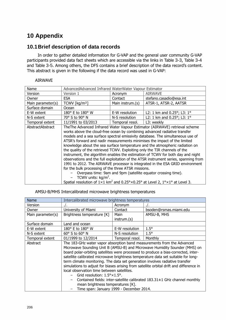
206

10 Appendix

10.1 Brief description of data records

In order to gather detailed information for G-VAP and the general user community G-VAP participants provided data fact sheets which are accessible via the links in Table 3-3, Table 3-4 and Table 3-5. Among others, the DFS contains a brief description of the data record’s content. This abstract is given in the following if the data record was used in G-VAP:

AIRWAVE

Name AdvancedAdvanced Infrared WaterWater Vapour Estimator Version Version 1 Acronym AIRWAVE Owner ESA Contact [email protected] Main parameter(s) TCWV [kg/m²] Main instrum.(s) ATSR-1, ATSR-2, AATSR Surface domain Ocean E-W extent 180° E to 180° W E-W resolution L2: 1 km and 0.25°; L3: 1° N-S extent 70° S to 90° N N-S resolution L2: 1 km and 0.25°; L3: 1° Temporal extent 11/1991 to 03/2013 Temporal resol. L3: weekly AbstractAbstract TheThe Advanced Infrared Water Vapour Estimator (AIRWAVE) retrieval scheme

works above the cloud-free ocean by combining advanced radiative transfer models and a sea surface spectral emissivity database. The simultaneous use of ATSR’s forward and nadir measurements minimises the impact of the limited knowledge about the sea surface temperature and the atmospheric radiation on the quality of the retrieved TCWV. Exploiting only the TIR channels of the instrument, the algorithm enables the estimation of TCWV for both day and night observations and the full exploitation of the ATSR instrument series, spanning from 1991 to 2012. The AIRWAVE processor is integrated in the ESA GRID environment for the bulk processing of the three ATSR missions.

− Overpass time: 9am and 9pm (satellite equator crossing time). − TCWV units: kg/m2.

Spatial resolution of 1×1 km2 and 0.25°×0.25° at Level 2, 1°×1° at Level 3.

AMSU-B/MHS Intercalibrated microwave brightness temperatures

Name Intercalibrated microwave brightness temperatures Version ./. Acronym ./. Owner University of Miami Contact [email protected] Main parameter(s) Brightness temperature [K] Main

instrum.(s) AMSU-B, MHS

Surface domain Land and ocean E-W extent 180° E to 180° W E-W resolution 1.5° N-S extent 60° S to 60° N N-S resolution 1.5° Temporal extent 01/1999 to 12/2014 Temporal resol. Monthly Abstract The 183-GHz water vapor absorption band measurements from the Advanced

Microwave Sounding Unit B (AMSU-B) and Microwave Humidity Sounder (MHS) on board polar-orbiting satellites were processed to produce a bias-corrected, inter-satellite calibrated microwave brightness temperature data set suitable for long-term climate monitoring. The data set generation involves radiative transfer simulations to adjust for biases arising from satellite orbital drift and difference in local observation time between satellites.

− Grid resolution: 1.5°×1.5°. − Contained fields: inter-satellite calibrated 183.31±1 GHz channel monthly

mean brightness temperatures [K]. − Time span: January 1999 - December 2014.

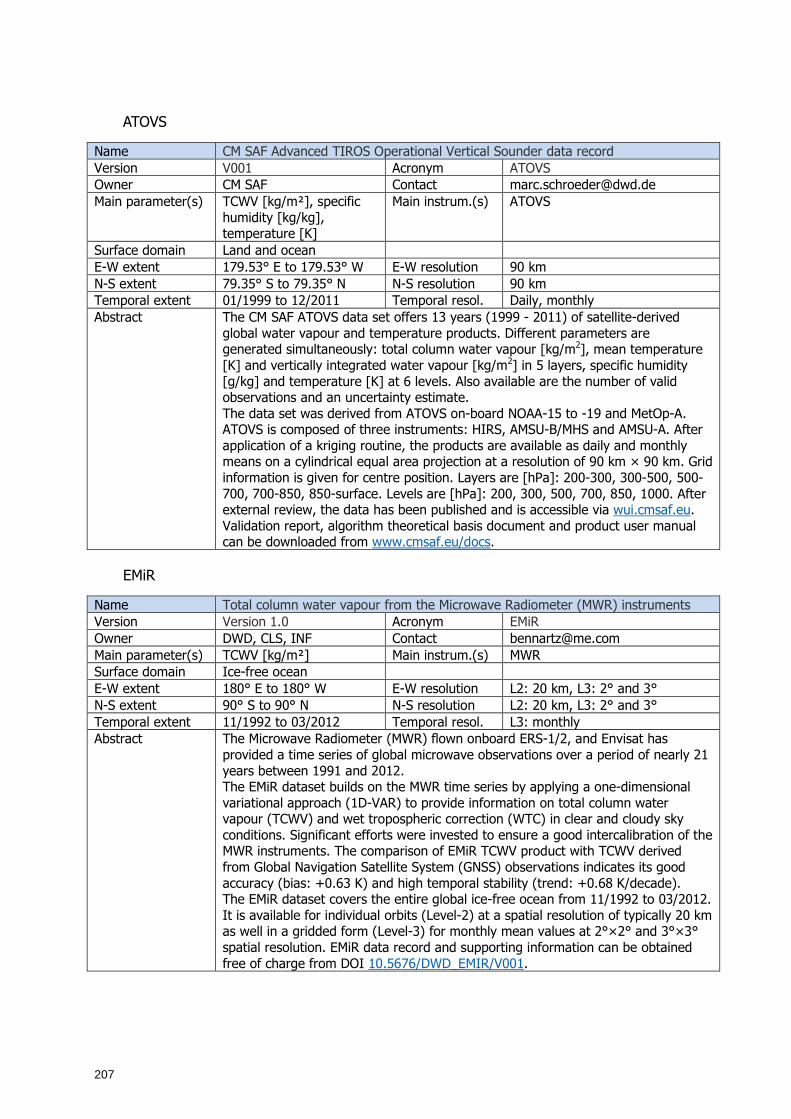
207

ATOVS

Name CM SAF Advanced TIROS Operational Vertical Sounder data record Version V001 Acronym ATOVS Owner CM SAF Contact [email protected] Main parameter(s) TCWV [kg/m²], specific

humidity [kg/kg], temperature [K]

Main instrum.(s) ATOVS

Surface domain Land and ocean E-W extent 179.53° E to 179.53° W E-W resolution 90 km N-S extent 79.35° S to 79.35° N N-S resolution 90 km Temporal extent 01/1999 to 12/2011 Temporal resol. Daily, monthly Abstract The CM SAF ATOVS data set offers 13 years (1999 - 2011) of satellite-derived

global water vapour and temperature products. Different parameters are generated simultaneously: total column water vapour [kg/m2], mean temperature [K] and vertically integrated water vapour [kg/m2] in 5 layers, specific humidity [g/kg] and temperature [K] at 6 levels. Also available are the number of valid observations and an uncertainty estimate. The data set was derived from ATOVS on-board NOAA-15 to -19 and MetOp-A. ATOVS is composed of three instruments: HIRS, AMSU-B/MHS and AMSU-A. After application of a kriging routine, the products are available as daily and monthly means on a cylindrical equal area projection at a resolution of 90 km × 90 km. Grid information is given for centre position. Layers are [hPa]: 200-300, 300-500, 500-700, 700-850, 850-surface. Levels are [hPa]: 200, 300, 500, 700, 850, 1000. After external review, the data has been published and is accessible via wui.cmsaf.eu. Validation report, algorithm theoretical basis document and product user manual can be downloaded from www.cmsaf.eu/docs.

EMiR

Name Total column water vapour from the Microwave Radiometer (MWR) instruments Version Version 1.0 Acronym EMiR Owner DWD, CLS, INF Contact [email protected] Main parameter(s) TCWV [kg/m²] Main instrum.(s) MWR Surface domain Ice-free ocean E-W extent 180° E to 180° W E-W resolution L2: 20 km, L3: 2° and 3° N-S extent 90° S to 90° N N-S resolution L2: 20 km, L3: 2° and 3° Temporal extent 11/1992 to 03/2012 Temporal resol. L3: monthly Abstract The Microwave Radiometer (MWR) flown onboard ERS-1/2, and Envisat has

provided a time series of global microwave observations over a period of nearly 21 years between 1991 and 2012. The EMiR dataset builds on the MWR time series by applying a one-dimensional variational approach (1D-VAR) to provide information on total column water vapour (TCWV) and wet tropospheric correction (WTC) in clear and cloudy sky conditions. Significant efforts were invested to ensure a good intercalibration of the MWR instruments. The comparison of EMiR TCWV product with TCWV derived from Global Navigation Satellite System (GNSS) observations indicates its good accuracy (bias: +0.63 K) and high temporal stability (trend: +0.68 K/decade). The EMiR dataset covers the entire global ice-free ocean from 11/1992 to 03/2012. It is available for individual orbits (Level-2) at a spatial resolution of typically 20 km as well in a gridded form (Level-3) for monthly mean values at 2°×2° and 3°×3° spatial resolution. EMiR data record and supporting information can be obtained free of charge from DOI 10.5676/DWD_EMIR/V001.

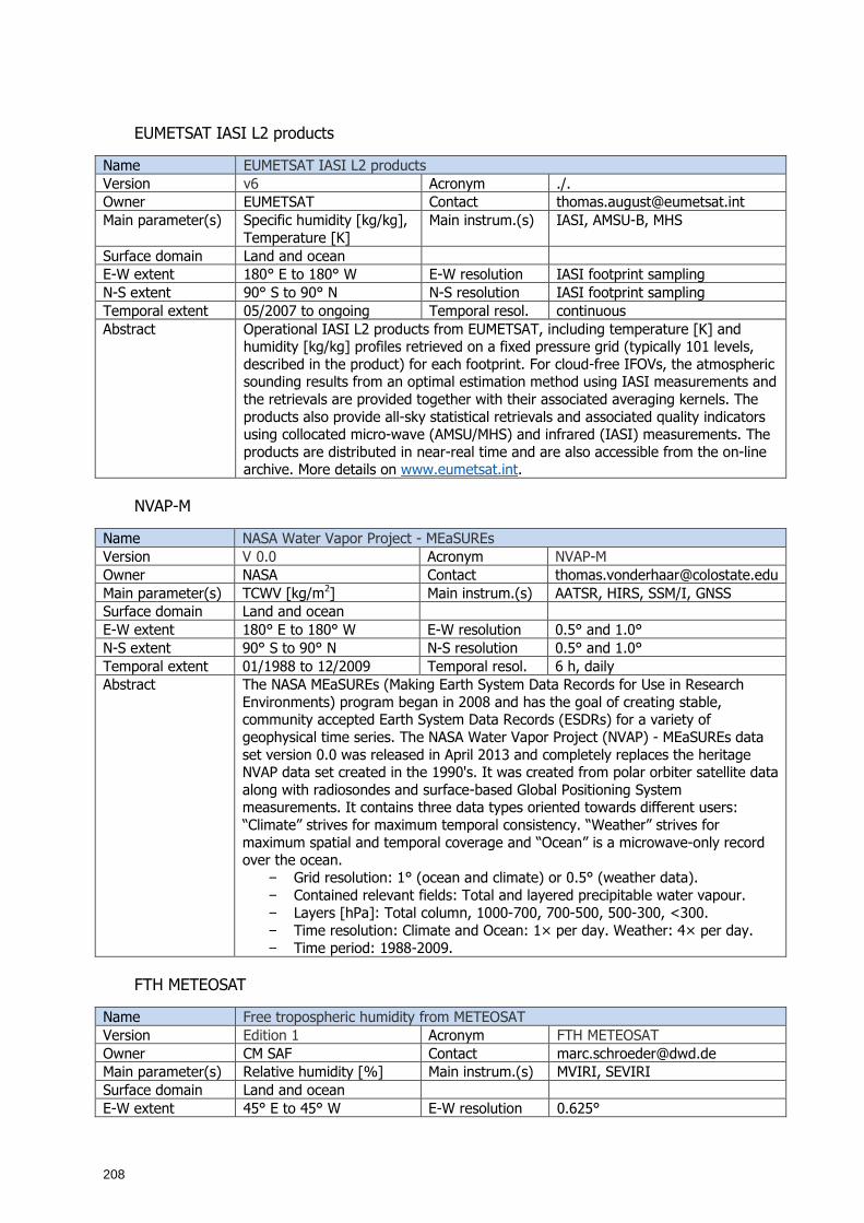
208

EUMETSAT IASI L2 products

Name EUMETSAT IASI L2 products Version v6 Acronym ./. Owner EUMETSAT Contact [email protected] Main parameter(s) Specific humidity [kg/kg],

Temperature [K] Main instrum.(s) IASI, AMSU-B, MHS

Surface domain Land and ocean E-W extent 180° E to 180° W E-W resolution IASI footprint sampling N-S extent 90° S to 90° N N-S resolution IASI footprint sampling Temporal extent 05/2007 to ongoing Temporal resol. continuous Abstract Operational IASI L2 products from EUMETSAT, including temperature [K] and

humidity [kg/kg] profiles retrieved on a fixed pressure grid (typically 101 levels, described in the product) for each footprint. For cloud-free IFOVs, the atmospheric sounding results from an optimal estimation method using IASI measurements and the retrievals are provided together with their associated averaging kernels. The products also provide all-sky statistical retrievals and associated quality indicators using collocated micro-wave (AMSU/MHS) and infrared (IASI) measurements. The products are distributed in near-real time and are also accessible from the on-line archive. More details on www.eumetsat.int.

NVAP-M

Name NASA Water Vapor Project - MEaSUREs Version V 0.0 Acronym NVAP-M Owner NASA Contact [email protected] Main parameter(s) TCWV [kg/m2] Main instrum.(s) AATSR, HIRS, SSM/I, GNSS Surface domain Land and ocean E-W extent 180° E to 180° W E-W resolution 0.5° and 1.0° N-S extent 90° S to 90° N N-S resolution 0.5° and 1.0° Temporal extent 01/1988 to 12/2009 Temporal resol. 6 h, daily Abstract The NASA MEaSUREs (Making Earth System Data Records for Use in Research

Environments) program began in 2008 and has the goal of creating stable, community accepted Earth System Data Records (ESDRs) for a variety of geophysical time series. The NASA Water Vapor Project (NVAP) - MEaSUREs data set version 0.0 was released in April 2013 and completely replaces the heritage NVAP data set created in the 1990's. It was created from polar orbiter satellite data along with radiosondes and surface-based Global Positioning System measurements. It contains three data types oriented towards different users: “Climate” strives for maximum temporal consistency. “Weather” strives for maximum spatial and temporal coverage and “Ocean” is a microwave-only record over the ocean.

− Grid resolution: 1° (ocean and climate) or 0.5° (weather data). − Contained relevant fields: Total and layered precipitable water vapour. − Layers [hPa]: Total column, 1000-700, 700-500, 500-300, <300. − Time resolution: Climate and Ocean: 1× per day. Weather: 4× per day. − Time period: 1988-2009.

FTH METEOSAT

Name Free tropospheric humidity from METEOSAT Version Edition 1 Acronym FTH METEOSAT Owner CM SAF Contact [email protected] Main parameter(s) Relative humidity [%] Main instrum.(s) MVIRI, SEVIRI Surface domain Land and ocean E-W extent 45° E to 45° W E-W resolution 0.625°

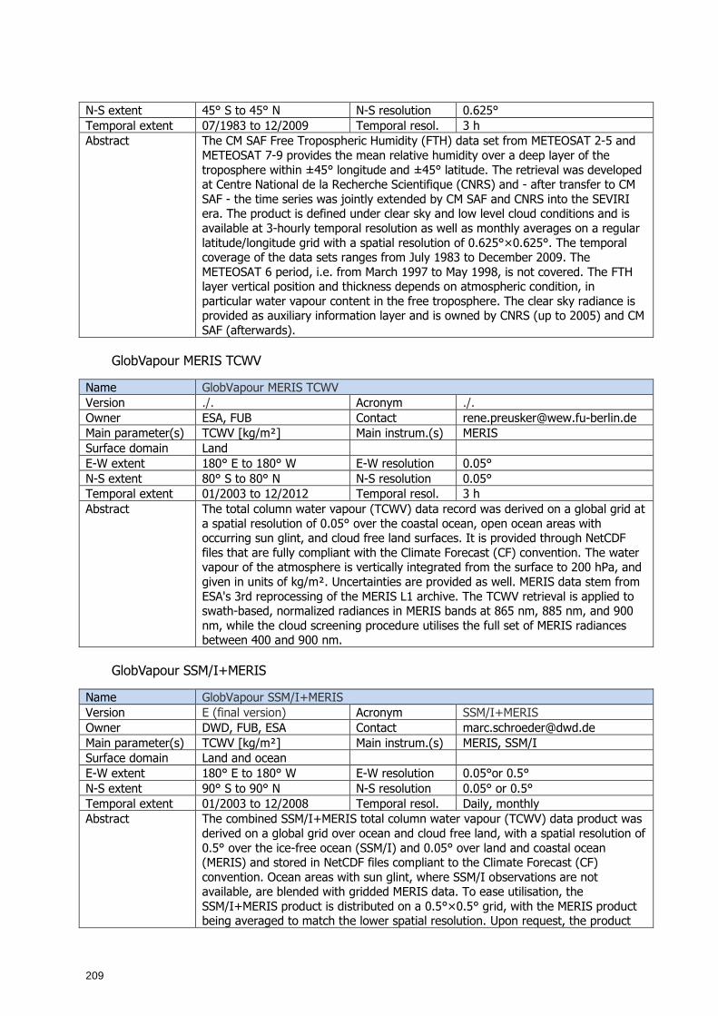
209

N-S extent 45° S to 45° N N-S resolution 0.625° Temporal extent 07/1983 to 12/2009 Temporal resol. 3 h Abstract The CM SAF Free Tropospheric Humidity (FTH) data set from METEOSAT 2-5 and

METEOSAT 7-9 provides the mean relative humidity over a deep layer of the troposphere within ±45° longitude and ±45° latitude. The retrieval was developed at Centre National de la Recherche Scientifique (CNRS) and - after transfer to CM SAF - the time series was jointly extended by CM SAF and CNRS into the SEVIRI era. The product is defined under clear sky and low level cloud conditions and is available at 3-hourly temporal resolution as well as monthly averages on a regular latitude/longitude grid with a spatial resolution of 0.625°×0.625°. The temporal coverage of the data sets ranges from July 1983 to December 2009. The METEOSAT 6 period, i.e. from March 1997 to May 1998, is not covered. The FTH layer vertical position and thickness depends on atmospheric condition, in particular water vapour content in the free troposphere. The clear sky radiance is provided as auxiliary information layer and is owned by CNRS (up to 2005) and CM SAF (afterwards).

GlobVapour MERIS TCWV

Name GlobVapour MERIS TCWV Version ./. Acronym ./. Owner ESA, FUB Contact [email protected] Main parameter(s) TCWV [kg/m²] Main instrum.(s) MERIS Surface domain Land E-W extent 180° E to 180° W E-W resolution 0.05° N-S extent 80° S to 80° N N-S resolution 0.05° Temporal extent 01/2003 to 12/2012 Temporal resol. 3 h Abstract The total column water vapour (TCWV) data record was derived on a global grid at

a spatial resolution of 0.05° over the coastal ocean, open ocean areas with occurring sun glint, and cloud free land surfaces. It is provided through NetCDF files that are fully compliant with the Climate Forecast (CF) convention. The water vapour of the atmosphere is vertically integrated from the surface to 200 hPa, and given in units of kg/m². Uncertainties are provided as well. MERIS data stem from ESA's 3rd reprocessing of the MERIS L1 archive. The TCWV retrieval is applied to swath-based, normalized radiances in MERIS bands at 865 nm, 885 nm, and 900 nm, while the cloud screening procedure utilises the full set of MERIS radiances between 400 and 900 nm.

GlobVapour SSM/I+MERIS

Name GlobVapour SSM/I+MERIS Version E (final version) Acronym SSM/I+MERIS Owner DWD, FUB, ESA Contact [email protected] Main parameter(s) TCWV [kg/m²] Main instrum.(s) MERIS, SSM/I Surface domain Land and ocean E-W extent 180° E to 180° W E-W resolution 0.05°or 0.5° N-S extent 90° S to 90° N N-S resolution 0.05° or 0.5° Temporal extent 01/2003 to 12/2008 Temporal resol. Daily, monthly Abstract The combined SSM/I+MERIS total column water vapour (TCWV) data product was

derived on a global grid over ocean and cloud free land, with a spatial resolution of 0.5° over the ice-free ocean (SSM/I) and 0.05° over land and coastal ocean (MERIS) and stored in NetCDF files compliant to the Climate Forecast (CF) convention. Ocean areas with sun glint, where SSM/I observations are not available, are blended with gridded MERIS data. To ease utilisation, the SSM/I+MERIS product is distributed on a 0.5°×0.5° grid, with the MERIS product being averaged to match the lower spatial resolution. Upon request, the product

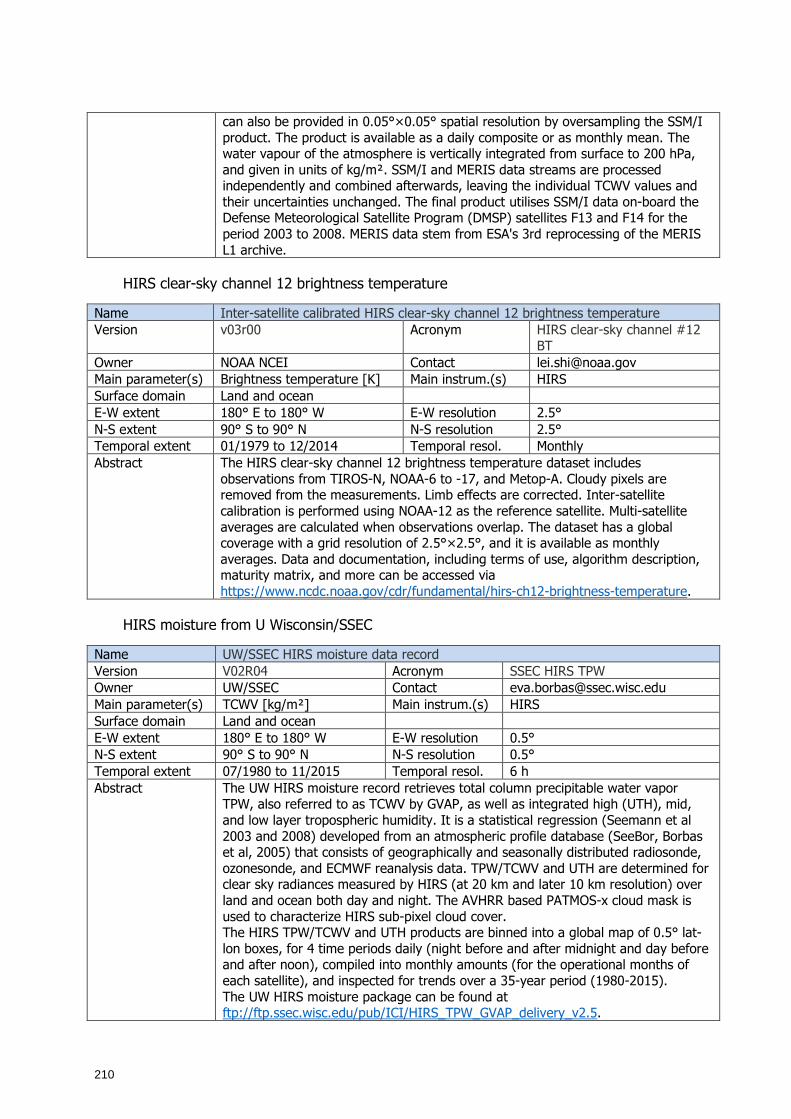
210

can also be provided in 0.05°×0.05° spatial resolution by oversampling the SSM/I product. The product is available as a daily composite or as monthly mean. The water vapour of the atmosphere is vertically integrated from surface to 200 hPa, and given in units of kg/m². SSM/I and MERIS data streams are processed independently and combined afterwards, leaving the individual TCWV values and their uncertainties unchanged. The final product utilises SSM/I data on-board the Defense Meteorological Satellite Program (DMSP) satellites F13 and F14 for the period 2003 to 2008. MERIS data stem from ESA's 3rd reprocessing of the MERIS L1 archive.

HIRS clear-sky channel 12 brightness temperature

Name Inter-satellite calibrated HIRS clear-sky channel 12 brightness temperature Version v03r00 Acronym HIRS clear-sky channel #12

BT Owner NOAA NCEI Contact [email protected] Main parameter(s) Brightness temperature [K] Main instrum.(s) HIRS Surface domain Land and ocean E-W extent 180° E to 180° W E-W resolution 2.5° N-S extent 90° S to 90° N N-S resolution 2.5° Temporal extent 01/1979 to 12/2014 Temporal resol. Monthly Abstract The HIRS clear-sky channel 12 brightness temperature dataset includes

observations from TIROS-N, NOAA-6 to -17, and Metop-A. Cloudy pixels are removed from the measurements. Limb effects are corrected. Inter-satellite calibration is performed using NOAA-12 as the reference satellite. Multi-satellite averages are calculated when observations overlap. The dataset has a global coverage with a grid resolution of 2.5°×2.5°, and it is available as monthly averages. Data and documentation, including terms of use, algorithm description, maturity matrix, and more can be accessed via https://www.ncdc.noaa.gov/cdr/fundamental/hirs-ch12-brightness-temperature.

HIRS moisture from U Wisconsin/SSEC

Name UW/SSEC HIRS moisture data record Version V02R04 Acronym SSEC HIRS TPW Owner UW/SSEC Contact [email protected] Main parameter(s) TCWV [kg/m²] Main instrum.(s) HIRS Surface domain Land and ocean E-W extent 180° E to 180° W E-W resolution 0.5° N-S extent 90° S to 90° N N-S resolution 0.5° Temporal extent 07/1980 to 11/2015 Temporal resol. 6 h Abstract The UW HIRS moisture record retrieves total column precipitable water vapor

TPW, also referred to as TCWV by GVAP, as well as integrated high (UTH), mid, and low layer tropospheric humidity. It is a statistical regression (Seemann et al 2003 and 2008) developed from an atmospheric profile database (SeeBor, Borbas et al, 2005) that consists of geographically and seasonally distributed radiosonde, ozonesonde, and ECMWF reanalysis data. TPW/TCWV and UTH are determined for clear sky radiances measured by HIRS (at 20 km and later 10 km resolution) over land and ocean both day and night. The AVHRR based PATMOS-x cloud mask is used to characterize HIRS sub-pixel cloud cover. The HIRS TPW/TCWV and UTH products are binned into a global map of 0.5° lat-lon boxes, for 4 time periods daily (night before and after midnight and day before and after noon), compiled into monthly amounts (for the operational months of each satellite), and inspected for trends over a 35-year period (1980-2015). The UW HIRS moisture package can be found at ftp://ftp.ssec.wisc.edu/pub/ICI/HIRS_TPW_GVAP_delivery_v2.5.

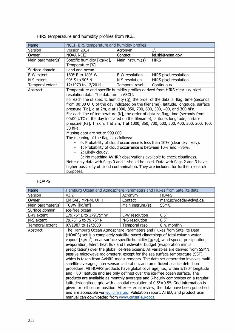
211

HIRS temperature and humidity profiles from NCEI

Name NCEI HIRS temperature and humidity profiles Version Version 2014 Acronym ./. Owner NOAA NCEI Contact [email protected] Main parameter(s) Specific humidity [kg/kg],

Temperature [K] Main instrum.(s) HIRS

Surface domain Land and ocean E-W extent 180° E to 180° W E-W resolution HIRS pixel resolution N-S extent 90° S to 90° N N-S resolution HIRS pixel resolution Temporal extent 12/1979 to 12/2014 Temporal resol. Continuous Abstract Temperature and specific humidity profiles derived from HIRS clear-sky pixel-

resolution data. The data are in ASCII. For each line of specific humidity (q), the order of the data is: flag, time (seconds from 00:00 UTC of the day indicated on the filename), latitude, longitude, surface pressure [Pa], q at 2m, q at 1000, 850, 700, 600, 500, 400, and 300 hPa. For each line of temperature [K], the order of data is: flag, time (seconds from 00:00 UTC of the day indicated on the filename), latitude, longitude, surface pressure [Pa], T_skin, T at 2m, T at 1000, 850, 700, 600, 500, 400, 300, 200, 100, 50 hPa. Missing data are set to 999.000. The meaning of the flag is as follows:

− 0: Probability of cloud occurrence is less than 10% (clear sky likely). − 1: Probability of cloud occurrence is between 10% and ~85%. − 2: Likely cloudy. − 3: No matching AVHRR observations available to check cloudiness.

Note: only data with flags 0 and 1 should be used. Data with flags 2 and 3 have higher possibility of cloud contamination. They are included for further research purposes.

HOAPS

Name Hamburg Ocean and Atmosphere Parameters and Fluxes from Satellite data Version V3.2 Acronym HOAPS Owner CM SAF, MPI-M, UHH Contact [email protected] Main parameter(s) TCWV [kg/m2] Main instrum.(s) SSM/I Surface domain Ice-free ocean E-W extent 179.75° E to 179.75° W E-W resolution 0.5° N-S extent 79.75° S to 79.75° N N-S resolution 0.5° Temporal extent 07/1987 to 12/2008 Temporal resol. 6 h, monthly Abstract The Hamburg Ocean Atmosphere Parameters and Fluxes from Satellite Data

(HOAPS) set is a completely satellite based climatology of total column water vapour [kg/m2], near surface specific humidity [g/kg], wind speed, precipitation, evaporation, latent heat flux and freshwater budget (evaporation minus precipitation) over the global ice-free oceans. All variables are derived from SSM/I passive microwave radiometers, except for the sea surface temperature (SST), which is taken from AVHRR measurements. The data set generation involves multi-satellite averages, inter-sensor calibration, and an efficient sea ice detection procedure. All HOAPS products have global coverage, i.e., within ±180° longitude and ±80° latitude and are only defined over the ice-free ocean surface. The products are available as monthly averages and 6-hourly composites on a regular latitude/longitude grid with a spatial resolution of 0.5°×0.5°. Grid information is given for cell centre position. After external review, the data have been published and are accessible via wui.cmsaf.eu. Validation report, ATBD, and product user manual can downloaded from www.cmsaf.eu/docs.

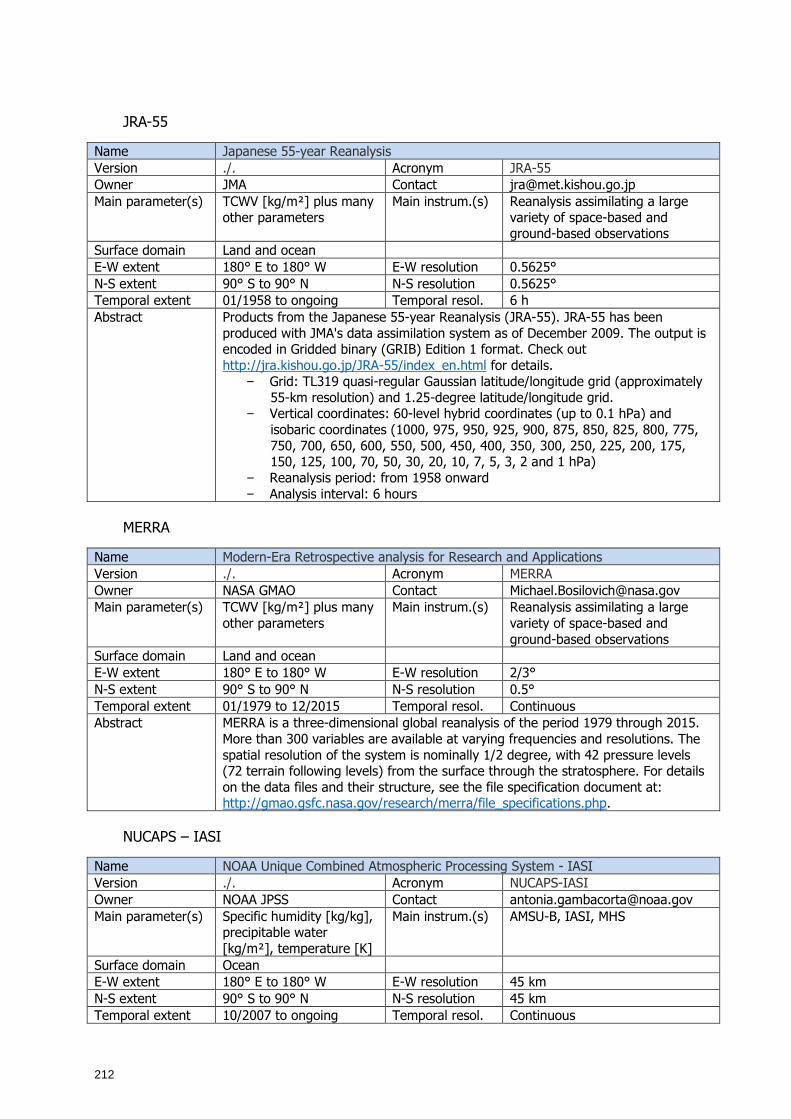
212

JRA-55

Name Japanese 55-year Reanalysis Version ./. Acronym JRA-55 Owner JMA Contact [email protected] Main parameter(s) TCWV [kg/m²] plus many

other parameters Main instrum.(s) Reanalysis assimilating a large

variety of space-based and ground-based observations

Surface domain Land and ocean E-W extent 180° E to 180° W E-W resolution 0.5625° N-S extent 90° S to 90° N N-S resolution 0.5625° Temporal extent 01/1958 to ongoing Temporal resol. 6 h Abstract Products from the Japanese 55-year Reanalysis (JRA-55). JRA-55 has been

produced with JMA's data assimilation system as of December 2009. The output is encoded in Gridded binary (GRIB) Edition 1 format. Check out http://jra.kishou.go.jp/JRA-55/index_en.html for details.

− Grid: TL319 quasi-regular Gaussian latitude/longitude grid (approximately 55-km resolution) and 1.25-degree latitude/longitude grid.

− Vertical coordinates: 60-level hybrid coordinates (up to 0.1 hPa) and isobaric coordinates (1000, 975, 950, 925, 900, 875, 850, 825, 800, 775, 750, 700, 650, 600, 550, 500, 450, 400, 350, 300, 250, 225, 200, 175, 150, 125, 100, 70, 50, 30, 20, 10, 7, 5, 3, 2 and 1 hPa)

− Reanalysis period: from 1958 onward − Analysis interval: 6 hours

MERRA

Name Modern-Era Retrospective analysis for Research and Applications Version ./. Acronym MERRA Owner NASA GMAO Contact [email protected] Main parameter(s) TCWV [kg/m²] plus many

other parameters Main instrum.(s) Reanalysis assimilating a large

variety of space-based and ground-based observations

Surface domain Land and ocean E-W extent 180° E to 180° W E-W resolution 2/3° N-S extent 90° S to 90° N N-S resolution 0.5° Temporal extent 01/1979 to 12/2015 Temporal resol. Continuous Abstract MERRA is a three-dimensional global reanalysis of the period 1979 through 2015.

More than 300 variables are available at varying frequencies and resolutions. The spatial resolution of the system is nominally 1/2 degree, with 42 pressure levels (72 terrain following levels) from the surface through the stratosphere. For details on the data files and their structure, see the file specification document at: http://gmao.gsfc.nasa.gov/research/merra/file_specifications.php.

NUCAPS – IASI

Name NOAA Unique Combined Atmospheric Processing System - IASI Version ./. Acronym NUCAPS-IASI Owner NOAA JPSS Contact [email protected] Main parameter(s) Specific humidity [kg/kg],

precipitable water [kg/m²], temperature [K]

Main instrum.(s) AMSU-B, IASI, MHS

Surface domain Ocean E-W extent 180° E to 180° W E-W resolution 45 km N-S extent 90° S to 90° N N-S resolution 45 km Temporal extent 10/2007 to ongoing Temporal resol. Continuous

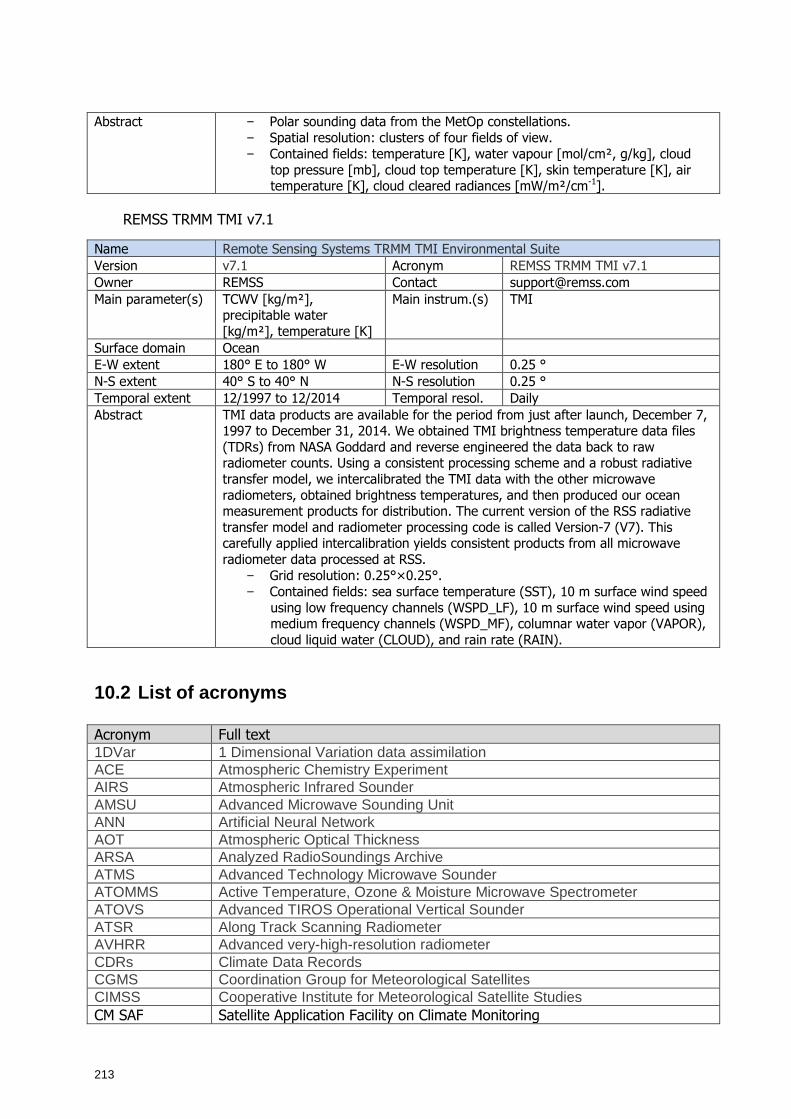
213

Abstract − Polar sounding data from the MetOp constellations. − Spatial resolution: clusters of four fields of view. − Contained fields: temperature [K], water vapour [mol/cm², g/kg], cloud

top pressure [mb], cloud top temperature [K], skin temperature [K], air temperature [K], cloud cleared radiances [mW/m²/cm-1].

REMSS TRMM TMI v7.1

Name Remote Sensing Systems TRMM TMI Environmental Suite Version v7.1 Acronym REMSS TRMM TMI v7.1 Owner REMSS Contact [email protected] Main parameter(s) TCWV [kg/m²],

precipitable water [kg/m²], temperature [K]

Main instrum.(s) TMI

Surface domain Ocean E-W extent 180° E to 180° W E-W resolution 0.25 ° N-S extent 40° S to 40° N N-S resolution 0.25 ° Temporal extent 12/1997 to 12/2014 Temporal resol. Daily Abstract TMI data products are available for the period from just after launch, December 7,

1997 to December 31, 2014. We obtained TMI brightness temperature data files (TDRs) from NASA Goddard and reverse engineered the data back to raw radiometer counts. Using a consistent processing scheme and a robust radiative transfer model, we intercalibrated the TMI data with the other microwave radiometers, obtained brightness temperatures, and then produced our ocean measurement products for distribution. The current version of the RSS radiative transfer model and radiometer processing code is called Version-7 (V7). This carefully applied intercalibration yields consistent products from all microwave radiometer data processed at RSS.

− Grid resolution: 0.25°×0.25°. − Contained fields: sea surface temperature (SST), 10 m surface wind speed

using low frequency channels (WSPD_LF), 10 m surface wind speed using medium frequency channels (WSPD_MF), columnar water vapor (VAPOR), cloud liquid water (CLOUD), and rain rate (RAIN).

10.2 List of acronyms Acronym Full text 1DVar 1 Dimensional Variation data assimilation ACE Atmospheric Chemistry Experiment AIRS Atmospheric Infrared Sounder AMSU Advanced Microwave Sounding Unit ANN Artificial Neural Network AOT Atmospheric Optical Thickness ARSA Analyzed RadioSoundings Archive ATMS Advanced Technology Microwave Sounder ATOMMS Active Temperature, Ozone & Moisture Microwave Spectrometer ATOVS Advanced TIROS Operational Vertical Sounder ATSR Along Track Scanning Radiometer AVHRR Advanced very-high-resolution radiometer CDRs Climate Data Records CGMS Coordination Group for Meteorological Satellites CIMSS Cooperative Institute for Meteorological Satellite Studies CM SAF Satellite Application Facility on Climate Monitoring

214

COSMIC Constellation Observing System for Meteorology, Ionosphere, and Climate CO2 Carbon Dioxide CrIS Cross-track Infrared Sounder (CrIS) DFS data fact sheet DoFS degrees of freedom for signal ECMWF European Centre for Medium-Range Weather Forecasts ECVs Essential Climate Variables ENSO El Nino/Southern Oscillation ERA Interim ECMWF Reanalysis FCDR Fundamental Climate Data Record FIDUCEO Fidelity and uncertainty in climate data records from Earth Observations FTH Free tropospheric Humidity GAIA-CLIM Gap Analysis for Integrated Atmospheric ECV CLImate Monitoring GCOS Global Climate Observing System GDAP GEWEX Data and Assessments Panel GEWEX Global Energy and Water Exchanges (a WCRP core project) GNSS Global Navigation Satellite System GOES Geostationary Operational Environmental Satellite GOME Global Ozone Monitoring Experiment GPS-RO Global Positioning System Radio Occultation GRAS Global Navigation Satellite System Receiver Atmospheric Sounding GRP GEWEX Radiation Panel GRUAN GCOS Reference Upper-Air Network G-VAP GEWEX Water Vapor Assessment HIRS High Resolution Infrared Radiation Sounder HOAPS Hamburg Ocean Atmosphere Parameters and Fluxes from Satellite Data IASI Infrared Atmospheric Sounder Interferometer IFS Integrated Forecasting System IFOV Instantaneous Field of View IPCC Intergovernmental Panel on Climate Change IR Infrared ISCCP International Satellite Cloud Climatology Project L1 Level 1 L2 Level 2 M02 Metop-A Satellite MHS Microwave Humidity Sounder MERIS Medium Resolution Imaging Spectrometer Instrument MODIS Moderate Resolution Imaging Spectroradiometer MVIRI Meteosat Visible and Infrared Radiation Imager MWR MicroWave Radiometer N12 NOAA-12 Satellite N14 NOAA-14 Satellite N15 NOAA-15 Satellite N16 NOAA-16 Satellite N17 NOAA-17 Satellite NCEI National Centers for Environmental Information NOA North Atlantic Oscillation NOAA National Oceanic and Atmospheric Administration NPROVS+ NOAA Products Validation System

215

NUCPS NOAA Unique Combined Atmospheric Processing System NWP Numerical Weather Prediction OLCI Ocean Land Colour Instrument on Sentinel 3 OSCAR Observing Systems Capability Analysis and Review Tool PDF Portable Document Format RH Relative Humidity RMS Root mean square RS92 Radiosonde Type RTM Radiative Transfer Model RTTOV Radiative Transfer for TOVS Forward Model SCIAMACHY Scanning Imaging Absorption Spectrometer for Atmospheric Chartography SEVIRI Spinning Enhanced Visible and Infrared Imager SHADOZ Southern Hemisphere ADditional OZonesondes SSM/I Special Sensor Microwave / Imager SNO Simultaneous Nadir Overpass TCWV Total Column Water Vapour SSM/I Special Sensor Microwave Imager SSMIS Special Sensor Microwave Imager Sounder TCWV Total Column Water Vapour TIROS Television and Infrared Observatory Spacecraft TMI TRMM Microwave Imager TMR TOPEX Microwave Radiometer TOA Top-Of-Atmosphere TOVS TIROS Operational Vertical Sounder TPW ARM Total Precipitable Water Vapour TTD time-to-detect UoL University Of Leicester UTH Total Column Water Vapour WMO World Meteorological Organisation WCRP World Climate Research Programme