Getis–Ord’s hot- and cold-spot statistics as a basis for multivariate spatial clustering of orchard tree data

Page 1

Computers and Electronics in Agriculture 111 (2015) 140–150

Contents lists available at ScienceDirect

Computers and Electronics in Agriculture

journal homepage: www.elsevier .com/locate /compag

Getis–Ord’s hot- and cold-spot statistics as a basis for multivariatespatial clustering of orchard tree data

http://dx.doi.org/10.1016/j.compag.2014.12.0110168-1699/� 2015 Elsevier B.V. All rights reserved.

⇑ Corresponding author at: Institute of Soil, Water and Environmental Sciences,Agricultural Research Organization, Gilat Research Center, Israel. Tel.: +972 86596875, +972 54 4570125; fax: +972 8 6596881.

E-mail address: [email protected] (A. Peeters).

Aviva Peeters a,b,⇑, Manuela Zude c, Jana Käthner c, Mustafa Ünlü d, Riza Kanber d, Amots Hetzroni e,Robin Gebbers c, Alon Ben-Gal a

a Institute of Soil, Water and Environmental Sciences, Agricultural Research Organization, Gilat Research Center, Israelb The Faculty of Food, Agriculture and Environmental Sciences, The Hebrew University of Jerusalem, Israelc Leibniz Institute for Agricultural Engineering Potsdam-Bornim e.V., Germanyd Faculty of Agriculture, University of Cukurova, Turkeye Institute of Agricultural Engineering, Agricultural Research Organization, Volcani Center, Israel

a r t i c l e i n f o

Article history:Received 25 March 2014Received in revised form 22 November 2014Accepted 12 December 2014

Keywords:GISHot-spot analysisk-means clusteringManagement zonesPrecision agricultureSpatial clustering

a b s t r a c t

Precision agriculture aims at sustainably optimizing the management of cultivated fields by addressingthe spatial variability found in crops and their environment. Spatial variability can be evaluated usingspatial cluster analysis, which partitions data into homogeneous groups, considering the geographicallocation of features and their spatial relationships. Spatial clustering methods evaluate the degree of spa-tial autocorrelation between features and quantify the statistical significance of identified clusters. Clus-tering of orchard data calls for an approach which is based on modeling point data, i.e. individual trees,which can be related to site-specific measurements. We present and evaluate a spatial clustering methodusing the Getis–Ord Gi

⁄ statistic to the analysis of tree-based data in an experimental orchard. We exam-ine the robustness of this method for the analysis of ‘‘hot-spots’’ (clusters of high data values) and ‘‘cold-spots’’ (clusters of low data values) in orchards and compare it to the k-means clustering algorithm, awidely-used aspatial method. We then present a novel approach which accounts for the spatial structureof data in a multivariate cluster analysis by combining the spatial Getis–Ord Gi

⁄ statistic with k-meansmultivariate clustering. The combined method improved results by both discriminating among featuresvalues as well as representing their spatial structure and therefore represents a superior technique foridentifying homogenous spatial clusters in orchards. This approach can be used as a tool for precisionmanagement of orchards by partitioning trees into management zones.

� 2015 Elsevier B.V. All rights reserved.

1. Introduction

The growing challenge to diminish the environmental footprintof farming while ensuring food security and economic viability ofagricultural practices has resulted in the development of precisionagriculture. Precision agriculture aims to sustainably optimize themanagement of cultivated fields by addressing the spatial variabil-ity found in crops and their environment. Soil properties and pastand present yield distributions are common examples of spatiallyvariable data with potential value for precision agriculture(Zhang et al., 2002). Knowledge regarding the form of distribution

and the extent of spatial variability of data can support site-specificmanagement of agricultural crops.

A well-established approach to recognize homogenous group-ings in data uses clustering or cluster analysis. This approach hasbeen extended to the analysis of spatial variability in agriculturalenvironments. Clustering consists of a group of methods whichaim at partitioning data into coherent or natural groups based onmeasures of similarity by maximizing within-cluster similaritiesas well as between-cluster differences (MacQueen, 1967). In gen-eral, clustering methods can be defined as either partitioning orhierarchical. Partitioning methods operate by dividing the entiredataset into n clusters, and hierarchical methods work by pairingindividual data points in a bottom-up or agglomerative process(Jain, 2010). Various clustering methods have been developedand adopted from other scientific fields to recognize homogenousgroupings in spatial agricultural data. Existing methods use either

Page 2

A. Peeters et al. / Computers and Electronics in Agriculture 111 (2015) 140–150 141

a univariate or multivariate approach of yield-defining variable(s)for recognizing homogenous groups in field data.

One of the most popular and well-established algorithms,widely applied in research domains such as data mining and pat-tern recognition, is k-means clustering (Ball and Hall, 1965;Lloyd, 1982; McQueen, 1967; Steinhaus, 1956; Theodoridis et al.,2010). While k-means has been used extensively in agriculture(Mucherino et al., 2009; Ortega and Santibáñez, 2007), its standardalgorithm is not very flexible and fuzzy clustering variants toimprove its use have therefore been developed (Fridgen et al.,2004; Fu et al., 2010; Kitchen et al., 2005; Vitharana et al., 2008;Yan et al., 2007). Additional clustering methods for agriculturaldata include the ISODATA method (Fraisse et al., 2001;Guastaferro et al., 2010), a non parametric approach developedby Aggelopoulou et al. (2013) and a hierarchical approach pre-sented by Fleming et al. (2000). A number of researchers have inte-grated k-means or fuzzy clustering with other algorithms (Córdobaet al., 2013; Davatgar et al., 2012; Fridgen et al., 2004).

In spite of the different clustering approaches that have beendeveloped, only a few make use of spatial constraints. Clusteringapproaches commonly rely only on the data attributes to recognizenatural groupings and partition data observations. To consider thespatial structure of data, clustering methods must integrate thegeographical location of objects and the spatial relationshipsbetween them directly into their mathematics (Cressie andWikle, 2011; Lloyd, 2010; Mitchell, 2005). By accounting for boththe differences in attribute values between features as well as forspatial location and relationships, spatial clustering methodsmodel spatial variability and uncertainties by quantifying the sta-tistical significance of recognized patterns and evaluate the degreeof clustering of observed spatial distribution.

Since agriculture is inherently a spatial phenomenon, in whichyield defining variables such as soil conditions, topography andmicroclimate vary in space, processes related to agricultural cropsand environments should be modeled using spatial methods. Somestudies, have introduced spatially constrained clustering methods,which limit class association to contiguous or proximal features inorder to form homogenous management zones. Spatially con-strained clustering uses aspatial clustering algorithms which aremodified by introducing constraints of spatial contiguity, for exam-ple by introducing spatial coordinates, Delaunay triangulation or Knearest neighbors (Gordon, 1996; Legendre and Legendre, 2012;Shatar and McBratney, 2001).

Other studies have examined different approaches to spatialclustering. Pedroso et al. (2010) for example, used a segmentationalgorithm, adopted from image processing, and compared it to k-means clustering and to spatially constrained k-means clusteringwith promising results, and Ping and Dobermann (2003) used aprior classification interpolation (PCF) approach preceding thecluster analysis and a post-classification filtering (PCF) approachto improve spatial contiguity of yield classes. Perry et al. (2010)have shown that tree properties in orchards exhibit spatial auto-correlation and that clustering results could be improved consider-ably by introducing spatial methods. A recent study by Córdobaet al. (2013), for example, compared the aspatial k-means algo-rithm with spatial clustering techniques, when applied to wheatand soybean crops. Their proposed approach combined spatialprincipal component analysis with fuzzy k-means (KM-sPC) toclassify elevation, soil and yield into spatial clusters. They assessedthe degree of within-field spatial variation (spatial autocorrelation)and came to the conclusion that adding the spatial dimensionimproved the clustering results and produced more contiguousgroups. Moreover, they concluded that under spatial autocorrela-tion, unconstrained fuzzy k-means clustering and classical princi-pal component analysis (PCA) were insufficient and were likelyto less successfully recognize spatial structure.

The majority of relevant agricultural research has concentratedon the use of aspatial clustering methods and particularly on theirapplication to field crops (Perry et al., 2010). While spatial cluster-ing methods have been applied in agriculture to address variousissues such as, crop disease (Cohen et al., 2011), yield potential(Lark, 1998; Perry et al., 2010) and soil fertility (Cohen et al.,2013; Yan et al., 2007), contributions attempting to apply spatialclustering techniques to tree-based data in orchards, are few andrather recent (Aggelopoulou et al., 2010, 2013; Kounatidis et al.,2008; Mann et al., 2010; Perry et al., 2010; Zaman andSchumann, 2006).

Since existing clustering approaches have been mainly devel-oped for annual crops they are based on either sampling continu-ous data, or on zonal data, such as yield per area, and do notnecessarily consider point-based data, such as from individualtrees. Attributes associated with tree crops can be either discreteor continuous. For example, tree size, flowering level and fruit yieldare examples of discrete variables associated with single trees only,while soil properties and consequential variables including wateror nutrient availability are continuous and occur throughout theentire orchard, even where trees are not present. Therefore, clus-tering of orchard data calls for an approach which is based on mod-eling point-based data i.e. individual trees and which can berelated to site-specific measurements.

We further investigated the conclusions on the significance ofspatial clustering in agriculture presented by studies such asCórdoba et al. (2013) and examined the application of spatial clus-tering to data gathered from individual trees in an orchard. Webegin by presenting a comparative study between two clusteringmethods; one aspatial and extensively-used and the other spatialand often applied to the analysis of point-based data such as crimeevents, rainfall modeling and disease cases, but rarely used in agri-culture, to recognize hot-spots (clusters of high data values) andcold-spots (clusters of low data values) in orchard data. We thenpresent a novel approach which combines spatial and aspatialmethods, particularly suitable for point-based data, and we evalu-ate its appropriateness for contiguous spatial cluster recognition inorchards.

2. Spatial vs. aspatial clustering

Aspatial clustering considers only the values of data points, inpartitioning the data into clusters. It does not account for the geo-graphical spatial context (spatial location and neighborhood), orfor the extent of spatial autocorrelation among data points(Aggelopoulou et al., 2013; Córdoba et al., 2013). However, spatialautocorrelation which measures the degree of similarity betweenneighboring features (data points), is an important concept in theanalysis of spatial data as it indicates whether features are spatiallydependent or independent (Cressie and Wikle, 2011; Lloyd, 2010).If features closer to each other tend to be more similar than fea-tures farther apart, they are considered to be spatially dependentand form a cluster (Lloyd, 2010). Another important aspect in theanalysis of spatial data is the representation of the spatial structureof the data in the actual computation of clusters. In order to com-pare the attribute values of each feature to the attributes of neigh-boring features the extent of the neighborhood surrounding eachfeature and the type of spatial interactions among features needsto be quantified. For example, if the influence of a feature on neigh-boring features decays with distance, or if there is a sphere of influ-ence beyond which features are not impacted, it should berepresented in the computation (Mitchell, 2005).

Traditional aspatial statistics is based on the assumptions thatobservations are independent of one another and identically dis-tributed (Chun and Griffith, 2013), and that relationships modeled

Page 3

142 A. Peeters et al. / Computers and Electronics in Agriculture 111 (2015) 140–150

are constant across the study area. However, spatial phenomenaexhibit both spatial dependence among features, and non-stationa-rity, i.e. spatial processes and relationships vary across the studyarea (Mitchell, 2005). Spatial statistical methods offer a range ofinferential tests that measure the degree to which the value of afeature’s attribute is similar to the attribute value of neighboringfeatures and can be used to quantify how spatial autocorrelationvaries locally and recognize spatial clusters. Similar to aspatialinferential statistics, spatial methods are evaluated within the con-text of a null hypothesis which states that attribute values do notexhibit local spatial clustering and can be rejected only if resultscan be considered statistically significant within a defined confi-dence level. Since a statistical index is calculated for each featurein the dataset, these can be mapped to indicate both the spatialvariability in local autocorrelation, and which features have statis-tically significant relationships with their neighbors. The contribu-tion of individual features on the identified pattern can beevaluated, thus enabling the recognition of outliers in the data.

The following presents the two clustering methods examined inthe current research: the aspatial k-means algorithm and the spa-tial Getis–Ord Gi

⁄ statistic (Getis and Ord, 1996; Mitchell, 2005; Ordand Getis, 1995).

2.1. Aspatial k-means clustering

The k-means algorithm is an iterative algorithm for partitioninga set of n data observations (x1,x2, . . .,xn) into homogenous k clus-ters (k 6 n) S = {S1,S2, . . .,Sk}. k-means minimizes the within-clustersum of squares (WCSS) and uses the squared Euclidean distancemetric (the distance between attribute values) as the measure ofsimilarity – Eq. (1) (Theodoridis et al., 2010):

S ¼ arg mins

Xk

i¼1

Xn

xj2Si

kxj � lik2 ð1Þ

where xj is the attribute value of the target feature, and li is themean of points in Si.

At its most basic form, k-means uses an iterative refinementprocess in which observations are assigned to a cluster with theobjective that each data observation will belong to the cluster withthe nearest mean (Jain, 2010). The centroid of each cluster subse-quently becomes the new mean and the process is repeated againuntil convergence to a local minimum is reached. The k-meansmethod is fast, straightforward and simple to implement, however,it suffers from a few drawbacks. The algorithm cannot assure con-vergence to the global minimum of S. Consequently, different ini-tializations of the algorithm might result in different finalclusters. Another critical drawback is the prerequisite for a user-defined parameter of the number of clusters (k) to be partitioned.A poor estimate will prevent the algorithm from recognizing theunderlying structure. The algorithm additionally is sensitive tothe presence of outliers (Theodoridis et al., 2010).

2.2. The spatial Getis–Ord Gi⁄ statistic

The Getis–Ord Gi⁄ statistic (Gi

⁄), known also as hot-spot analysis(Getis and Ord, 1992, 1996; Mitchell, 2005; Ord and Getis, 1995) isa method for analyzing the location related tendency (clustering)in the attributes of spatial data (points or areas). Developed inthe mid 1990s, this method has commonly been used in rainfalland epidemic modeling and has been applied in recent years inagriculture as well (Chopin and Blazy, 2013; Kounatidis et al.,2008; Rud et al., 2013). The method is an adaptation of the GeneralG-statistic (Getis and Ord, 1992), a global method for quantifyingthe degree of spatial autocorrelation over an area. The General G-statistic computes a single statistic for the entire study area, while

the Gi⁄ statistic serves as an indicator for local autocorrelation, i.e. it

measures how spatial autocorrelation varies locally over the studyarea and computes a statistic for each data point. The method eval-uates the degree to which each feature is surrounded by featureswith similarly high or low values within a specified geographicaldistance (neighborhood) – Eq. (2).

G�i ðdÞ ¼P

jwijðdÞxjPjxj

ð2Þ

where Gi⁄(d) is the local G-statistic for a feature (i) within a distance

(d), xj is the attribute value of each neighbor, and wij is the spatialweight for the target-neighbor i and j pair. Typically, the spatial dis-tances between observations at points are calculated by the Euclid-ean norm. The spatial weights wij are the n � n elements of thespatial weight matrix W, where n is the number of observations.There are several possible types of W (Haining, 2003). A simpleform, commonly used in the Gi

⁄ statistic is a matrix derived from athreshold (d) for the distance between xi and xj (Chun andGriffith, 2013; Ord and Getis, 1995). The threshold parameter ddefines the distance within which all locations are considered asneighbors (indicated by 1 in the W matrix), and beyond which alllocations are not neighbors (indicated by 0 in the W matrix or byweights which diminish with distance). Gi

⁄ is only applicable forpositive x.

The statistical significance in the degree of local autocorrelationbetween each feature and its neighbors is assessed by the z-scoretest. The z-score and p-value reported for each feature indicatewhether spatial clustering of either high or low values, or a spatialoutlier is more pronounced than one would expect in a randomdistribution, i.e. whether or not it is possible to reject the nullhypothesis of no apparent clustering.

In order to improve statistical testing, Ord and Getis (1995)developed a z-transformed form of Gi

⁄ by taking the statistic Gi⁄(d)

minus its expectation, divided by the square root of its variance.Using the same symbology, this z-transformation, termed the stan-dardized Gi

⁄ statistic is given in Eq. (3). The Gi⁄ statistic computed by

ArcGIS (ESRI, Redlands, CA, USA) uses this version of Gi⁄ in which

the Gi⁄ index is combined with the z-score into one single index.

The statistic, still called Gi⁄, reports a z-score and p-value for each

single feature.

G�i ðdÞ ¼P

jwijðdÞxj � XP

jwijðdÞ

s

ffiffiffiffiffiffiffiffiffiffiffiffiffiffiffiffiffiffiffiffiffiffiffiffiffiffiffiffiffiffiffiffiffiffiffiffiffinP

jw2

ij�P

jwijðdÞ

� �2

n�1

s ð3Þ

with

X ¼P

ixj

n

and

S ¼

ffiffiffiffiffiffiffiffiffiffiffiffiffiffiffiffiffiffiffiffiffiffiffiffiffiffiPjx

2j

n� ðXÞ2

s

where Gi⁄(d) is computed for feature (i) at a distance (d) standard-

ized as a z-score. xj is the attribute value of each neighbor, wij isthe spatial weight for the target-neighbor i and j pair and n is thetotal number of samples in the dataset. A Euclidean method is usedto calculate the geographical distances from each feature to itsneighboring features. The spatial structure of the data (neighbor-hood and relationships between features) is represented and quan-tified as in Eq. (4) by using the spatial weight (wij), calculated basedon a spatial weight matrix. The spatial weight matrix is an n � n table(n equals to the number of features in the dataset), which surroundseach feature, in which each value in the matrix is a weight repre-senting the relationship between a pair of features in the dataset.

Page 4

A. Peeters et al. / Computers and Electronics in Agriculture 111 (2015) 140–150 143

The Gi⁄ statistic introduced by Getis and Ord in 1995 extended the

family of G statistics to incorporate non-binary weight matricesand account for a wij(d) which varies with distance. For exampleweights can be assigned based on an inverse distance weightsmatrix (distance decay), or a combination of the inverse distanceand the fixed distance band models (similar to a fixed distance witha fuzzy boundary). Defining the distance band (d) is parametric anddepends on the nature of the dataset and on the phenomenon mod-eled and should be defined according to the distance in which spa-tial autocorrelation peaks. This can be modeled by applying aniterative and data-driven process which examines how spatialautocorrelation varies at different distances.

The output of the Gi⁄ statistic is a map indicating the location of

spatial clusters in the study area. Positive values of Gi⁄ denote spa-

tial dependence among high values. Negative values of Gi⁄ indicate

spatial dependence for low values. The degree of clustering and itsstatistical significance is evaluated based on a confidence level andon output z-scores. These define whether a data point belongs to ahot-spot (spatial cluster of high data values), cold-spot (spatialcluster of low data values) or an outlier (a high data value sur-rounded by low data values or vice versa).

3. Materials and methods

3.1. Data collection

Data was collected in 2011 and 2012 from individualgrapefruit trees (Citrus paradise, cv. Rio Red) within an irrigated

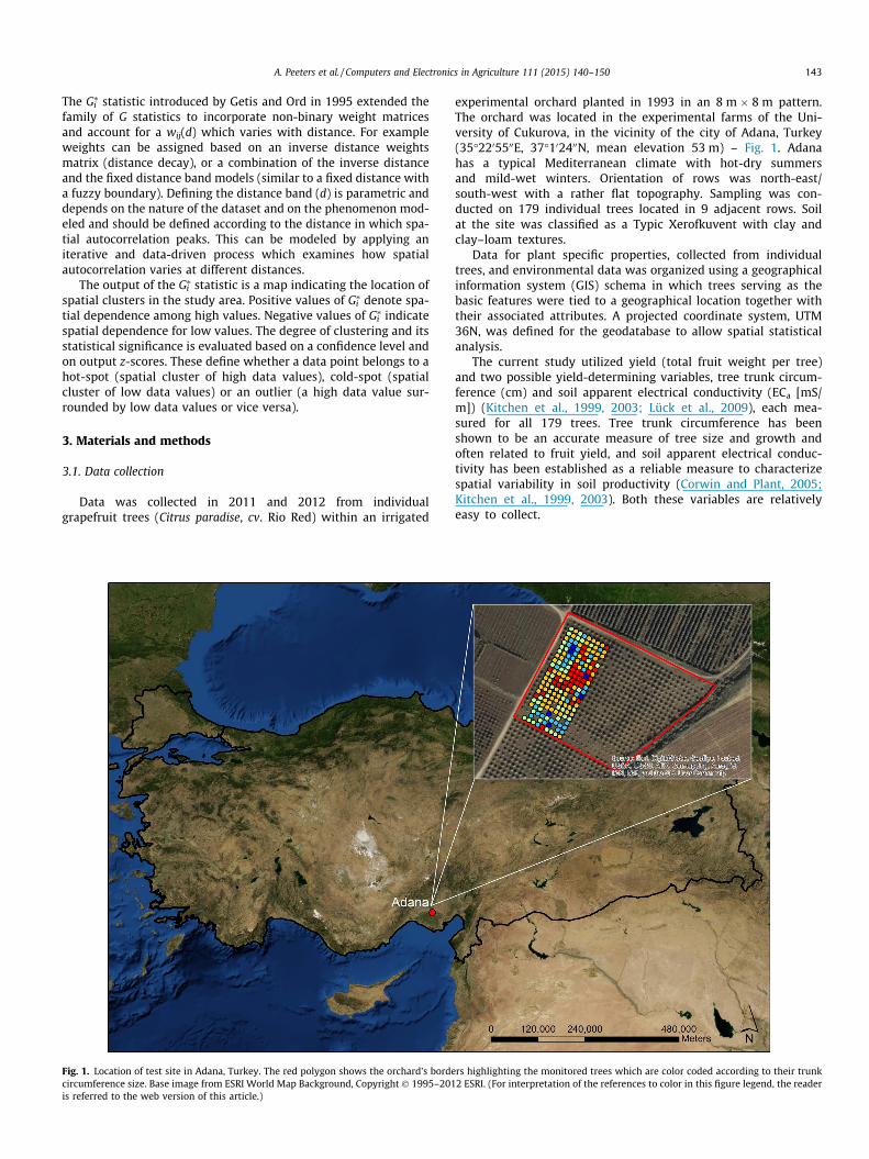
Fig. 1. Location of test site in Adana, Turkey. The red polygon shows the orchard’s bordecircumference size. Base image from ESRI World Map Background, Copyright � 1995–201is referred to the web version of this article.)

experimental orchard planted in 1993 in an 8 m � 8 m pattern.The orchard was located in the experimental farms of the Uni-versity of Cukurova, in the vicinity of the city of Adana, Turkey(35�2205500E, 37�102400N, mean elevation 53 m) – Fig. 1. Adanahas a typical Mediterranean climate with hot-dry summersand mild-wet winters. Orientation of rows was north-east/south-west with a rather flat topography. Sampling was con-ducted on 179 individual trees located in 9 adjacent rows. Soilat the site was classified as a Typic Xerofkuvent with clay andclay–loam textures.

Data for plant specific properties, collected from individualtrees, and environmental data was organized using a geographicalinformation system (GIS) schema in which trees serving as thebasic features were tied to a geographical location together withtheir associated attributes. A projected coordinate system, UTM36N, was defined for the geodatabase to allow spatial statisticalanalysis.

The current study utilized yield (total fruit weight per tree)and two possible yield-determining variables, tree trunk circum-ference (cm) and soil apparent electrical conductivity (ECa [mS/m]) (Kitchen et al., 1999, 2003; Lück et al., 2009), each mea-sured for all 179 trees. Tree trunk circumference has beenshown to be an accurate measure of tree size and growth andoften related to fruit yield, and soil apparent electrical conduc-tivity has been established as a reliable measure to characterizespatial variability in soil productivity (Corwin and Plant, 2005;Kitchen et al., 1999, 2003). Both these variables are relativelyeasy to collect.

rs highlighting the monitored trees which are color coded according to their trunk2 ESRI. (For interpretation of the references to color in this figure legend, the reader

Page 5

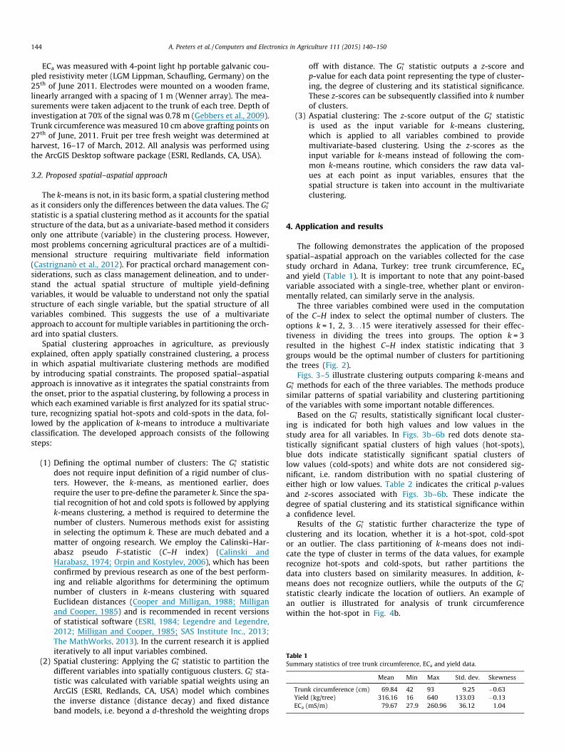
Table 1Summary statistics of tree trunk circumference, ECa and yield data.

Mean Min Max Std. dev. Skewness

Trunk circumference (cm) 69.84 42 93 9.25 �0.63Yield (kg/tree) 316.16 16 640 133.03 �0.13ECa (mS/m) 79.67 27.9 260.96 36.12 1.04

144 A. Peeters et al. / Computers and Electronics in Agriculture 111 (2015) 140–150

ECa was measured with 4-point light hp portable galvanic cou-pled resistivity meter (LGM Lippman, Schaufling, Germany) on the25th of June 2011. Electrodes were mounted on a wooden frame,linearly arranged with a spacing of 1 m (Wenner array). The mea-surements were taken adjacent to the trunk of each tree. Depth ofinvestigation at 70% of the signal was 0.78 m (Gebbers et al., 2009).Trunk circumference was measured 10 cm above grafting points on27th of June, 2011. Fruit per tree fresh weight was determined atharvest, 16–17 of March, 2012. All analysis was performed usingthe ArcGIS Desktop software package (ESRI, Redlands, CA, USA).

3.2. Proposed spatial–aspatial approach

The k-means is not, in its basic form, a spatial clustering methodas it considers only the differences between the data values. The Gi

⁄

statistic is a spatial clustering method as it accounts for the spatialstructure of the data, but as a univariate-based method it considersonly one attribute (variable) in the clustering process. However,most problems concerning agricultural practices are of a multidi-mensional structure requiring multivariate field information(Castrignanò et al., 2012). For practical orchard management con-siderations, such as class management delineation, and to under-stand the actual spatial structure of multiple yield-definingvariables, it would be valuable to understand not only the spatialstructure of each single variable, but the spatial structure of allvariables combined. This suggests the use of a multivariateapproach to account for multiple variables in partitioning the orch-ard into spatial clusters.

Spatial clustering approaches in agriculture, as previouslyexplained, often apply spatially constrained clustering, a processin which aspatial multivariate clustering methods are modifiedby introducing spatial constraints. The proposed spatial–aspatialapproach is innovative as it integrates the spatial constraints fromthe onset, prior to the aspatial clustering, by following a process inwhich each examined variable is first analyzed for its spatial struc-ture, recognizing spatial hot-spots and cold-spots in the data, fol-lowed by the application of k-means to introduce a multivariateclassification. The developed approach consists of the followingsteps:

(1) Defining the optimal number of clusters: The Gi⁄ statistic

does not require input definition of a rigid number of clus-ters. However, the k-means, as mentioned earlier, doesrequire the user to pre-define the parameter k. Since the spa-tial recognition of hot and cold spots is followed by applyingk-means clustering, a method is required to determine thenumber of clusters. Numerous methods exist for assistingin selecting the optimum k. These are much debated and amatter of ongoing research. We employ the Calinski–Har-abasz pseudo F-statistic (C–H index) (Calinski andHarabasz, 1974; Orpin and Kostylev, 2006), which has beenconfirmed by previous research as one of the best perform-ing and reliable algorithms for determining the optimumnumber of clusters in k-means clustering with squaredEuclidean distances (Cooper and Milligan, 1988; Milliganand Cooper, 1985) and is recommended in recent versionsof statistical software (ESRI, 1984; Legendre and Legendre,2012; Milligan and Cooper, 1985; SAS Institute Inc., 2013;The MathWorks, 2013). In the current research it is appliediteratively to all input variables combined.

(2) Spatial clustering: Applying the Gi⁄ statistic to partition the

different variables into spatially contiguous clusters. Gi⁄ sta-

tistic was calculated with variable spatial weights using anArcGIS (ESRI, Redlands, CA, USA) model which combinesthe inverse distance (distance decay) and fixed distanceband models, i.e. beyond a d-threshold the weighting drops

off with distance. The Gi⁄ statistic outputs a z-score and

p-value for each data point representing the type of cluster-ing, the degree of clustering and its statistical significance.These z-scores can be subsequently classified into k numberof clusters.

(3) Aspatial clustering: The z-score output of the Gi⁄ statistic

is used as the input variable for k-means clustering,which is applied to all variables combined to providemultivariate-based clustering. Using the z-scores as theinput variable for k-means instead of following the com-mon k-means routine, which considers the raw data val-ues at each point as input variables, ensures that thespatial structure is taken into account in the multivariateclustering.

4. Application and results

The following demonstrates the application of the proposedspatial–aspatial approach on the variables collected for the casestudy orchard in Adana, Turkey: tree trunk circumference, ECa

and yield (Table 1). It is important to note that any point-basedvariable associated with a single-tree, whether plant or environ-mentally related, can similarly serve in the analysis.

The three variables combined were used in the computationof the C–H index to select the optimal number of clusters. Theoptions k = 1, 2, 3. . .15 were iteratively assessed for their effec-tiveness in dividing the trees into groups. The option k = 3resulted in the highest C–H index statistic indicating that 3groups would be the optimal number of clusters for partitioningthe trees (Fig. 2).

Figs. 3–5 illustrate clustering outputs comparing k-means andGi⁄ methods for each of the three variables. The methods produce

similar patterns of spatial variability and clustering partitioningof the variables with some important notable differences.

Based on the Gi⁄ results, statistically significant local cluster-

ing is indicated for both high values and low values in thestudy area for all variables. In Figs. 3b–6b red dots denote sta-tistically significant spatial clusters of high values (hot-spots),blue dots indicate statistically significant spatial clusters oflow values (cold-spots) and white dots are not considered sig-nificant, i.e. random distribution with no spatial clustering ofeither high or low values. Table 2 indicates the critical p-valuesand z-scores associated with Figs. 3b–6b. These indicate thedegree of spatial clustering and its statistical significance withina confidence level.

Results of the Gi⁄ statistic further characterize the type of

clustering and its location, whether it is a hot-spot, cold-spotor an outlier. The class partitioning of k-means does not indi-cate the type of cluster in terms of the data values, for examplerecognize hot-spots and cold-spots, but rather partitions thedata into clusters based on similarity measures. In addition, k-means does not recognize outliers, while the outputs of the Gi

⁄

statistic clearly indicate the location of outliers. An example ofan outlier is illustrated for analysis of trunk circumferencewithin the hot-spot in Fig. 4b.

Page 6

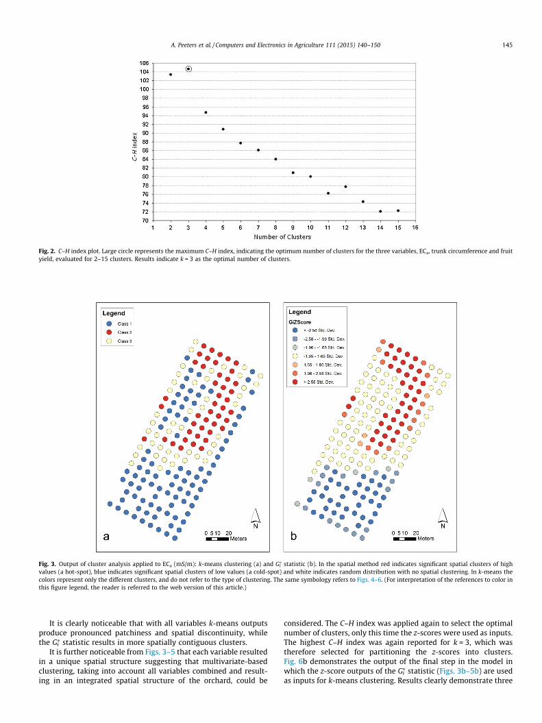
Fig. 2. C–H index plot. Large circle represents the maximum C–H index, indicating the optimum number of clusters for the three variables, ECa, trunk circumference and fruityield, evaluated for 2–15 clusters. Results indicate k = 3 as the optimal number of clusters.

Fig. 3. Output of cluster analysis applied to ECa (mS/m): k-means clustering (a) and Gi⁄ statistic (b). In the spatial method red indicates significant spatial clusters of high

values (a hot-spot), blue indicates significant spatial clusters of low values (a cold-spot) and white indicates random distribution with no spatial clustering. In k-means thecolors represent only the different clusters, and do not refer to the type of clustering. The same symbology refers to Figs. 4–6. (For interpretation of the references to color inthis figure legend, the reader is referred to the web version of this article.)

A. Peeters et al. / Computers and Electronics in Agriculture 111 (2015) 140–150 145

It is clearly noticeable that with all variables k-means outputsproduce pronounced patchiness and spatial discontinuity, whilethe Gi

⁄ statistic results in more spatially contiguous clusters.It is further noticeable from Figs. 3–5 that each variable resulted

in a unique spatial structure suggesting that multivariate-basedclustering, taking into account all variables combined and result-ing in an integrated spatial structure of the orchard, could be

considered. The C–H index was applied again to select the optimalnumber of clusters, only this time the z-scores were used as inputs.The highest C–H index was again reported for k = 3, which wastherefore selected for partitioning the z-scores into clusters.Fig. 6b demonstrates the output of the final step in the model inwhich the z-score outputs of the Gi

⁄ statistic (Figs. 3b–5b) are usedas inputs for k-means clustering. Results clearly demonstrate three

Page 7

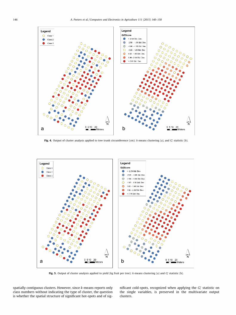
Fig. 4. Output of cluster analysis applied to tree trunk circumference (cm): k-means clustering (a), and Gi⁄ statistic (b).

Fig. 5. Output of cluster analysis applied to yield (kg fruit per tree): k-means clustering (a) and Gi⁄ statistic (b).

146 A. Peeters et al. / Computers and Electronics in Agriculture 111 (2015) 140–150

spatially contiguous clusters. However, since k-means reports onlyclass numbers without indicating the type of cluster, the questionis whether the spatial structure of significant hot-spots and of sig-

nificant cold-spots, recognized when applying the Gi⁄ statistic on

the single variables, is preserved in the multivariate outputclusters.

Page 8

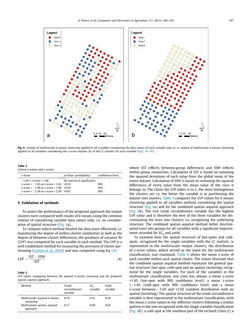
Fig. 6. Output of multivariate k-means clustering applied to all variables considering the data values of each variable only (a) vs. output of multivariate k-means clusteringapplied to all variables considering the z-score outputs (b) of the Gi

⁄ statistic for each variable (Figs. 3b–5b).

Table 2Critical p-values and z-scores.

z-Score p-Value (probability) Confidence level

�1.96 < z-score > 1.96 No statistical significancez-score < �1.65 or z-score > 1.65 <0.10 90%z-score < �1.96 or z-score > 1.96 <0.05 95%z-score < �2.58 or z-score > 2.58 <0.01 99%

A. Peeters et al. / Computers and Electronics in Agriculture 111 (2015) 140–150 147

5. Validation of methods

To assess the performance of the proposed approach the outputclusters were compared with results of k-means using the commonroutine of considering variable data values only; i.e. no consider-ation of spatial structure (Fig. 6a).

To compare which method divided the data most effectively i.e.maximizing the degree of within-cluster similarities as well as thedegree of between-cluster differences, the goodness of variance fit(GVF) was computed for each variable in each method. The GVF is awell established method for measuring the precision of cluster par-titioning (Cauvin et al., 2010) and was computed using Eq. (4):

GVF ¼ SST � SSWSST

ð4Þ

Table 3GVF values comparing between the aspatial k-means clustering and the proposedspatial–aspatial approach.

Method Trunkcircumferencevariable

ECa

variableYieldvariable

Multivariate aspatial k-meansclustering

0.74 0.41 0.39

Multivariate spatial–aspatialapproach

0.77 0.60 0.64

where SST reflects between-group differences and SSW reflectswithin-group similarities. Calculation of SST is based on summingthe squared deviations of each value from the global mean of theentire dataset. Calculation of SSW is based on summing the squareddifferences of every value from the mean value of the class itbelongs to. The closer the GVF index is to 1, the more homogenousthe clusters are i.e. the better the variable is at partitioning thedataset into clusters. Table 3 compares the GVF values for k-meansclustering applied to all variables without considering the spatialstructure (Fig. 6a) and for the combined spatial–aspatial approach(Fig. 6b). The tree trunk circumference variable has the highestGVF value and is therefore the best of the three variables for dis-criminating the trees into clusters, i.e. recognizing the underlyingstructure. The combined spatial–aspatial method better discrimi-nated trees into groups for all variables with a significant improve-ment recorded for ECa and yield.

To examine how the spatial structure of hot-spots and cold-spots, recognized for the single variables with the Gi

⁄ statistic, isrepresented in the multivariate output clusters, the distributionof z-score values, which served as the input for the multivariateclassification, was examined. Table 4 shows the mean z-score ofeach variable within each spatial cluster. The values illustrate thatthe combined spatial–aspatial method maintains the general spa-tial structure (hot-spot, cold-spot and no spatial clustering) recog-nized for the single variables. For each of the variables in themultivariate classification, one class has always a mean z-score>1.65 (hot-spot with 90% confidence level), a mean z-score<�1.65 (cold-spot with 90% confidence level) and a meanz-score between �1.65 and +1.65 (random distribution with nospatial clustering). The spatial structure of the trunk circumferencevariable is best represented in the multivariate classification, withthe mean z-score values in the different clusters following a similarpattern to the one recognized with the single variable classification(Fig. 4b): a cold-spot at the southern part of the orchard (Class 2), a

Page 9

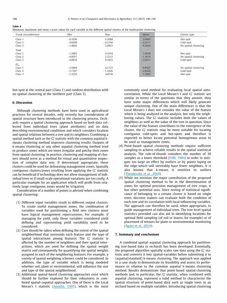
Table 4Minimum, maximum and mean z-score values for each variable in the different spatial clusters of the multivariate clustering.

148 A. Peeters et al. / Computers and Electronics in Agriculture 111 (2015) 140–150

hot-spot at the central part (Class 1) and random distribution withno spatial clustering at the northern part (Class 3).

6. Discussion

Although clustering methods have been used in agriculturalpractices for several decades, only recently has consideration ofspatial structure been introduced in the clustering process. Orch-ards require a spatial clustering approach based on both data col-lected from individual trees (plant attributes) and on datadescribing environmental conditions and which considers locationand spatial relations between a tree and its neighbors. Combining aspatial method such as the Gi

⁄ statistic with the common aspatial k-means clustering method improves clustering results. Outputs ofk-means clustering or any other aspatial clustering method tendto produce zones which are more irregular and patchy then zonesfrom spatial clustering. In practice, clustering and mapping of clus-ters should serve as a method for visual and quantitative inspec-tion of complex data sets. If determined appropriate, theseclusters could be used for delineating management zones. Spatiallycontiguous clusters/zones resulting from applying the Gi

⁄ statisticcan be beneficial if technology does not allow management of indi-vidual trees or if small-scale operational variations are too costly. Aparticular example for an application which will profit from rela-tively large contiguous zones would be irrigation.

Consideration of a number of points is advised when combiningspatial clustering:

(1) Different input variables result in different output clusters.To create useful management zones, the combination ofvariables used for partitioning a field into clusters musthave logical management repercussions. For example, ifmanaging for yield, only those variables considered yielddefining and representing yield variability need to beconsidered.

(2) Care should be taken when defining the extent of the spatialneighborhood that surrounds each feature and the type ofspatial interactions among features. The Gi

⁄ statistic isaffected by the number of neighbors and their spatial inter-actions, which are used for defining the spatial weightmatrix and consequently for quantifying the spatial weightsassigned to each of the neighboring features. For example, avariety of spatial weighting schemes could be considered. Inaddition, the type of variable which is being modeledwhether soil, plant or environmental, will influence the sizeand type of the spatial neighborhood.

(3) Additional spatial-based clustering approaches exist whichshould be further explored for their robustness in com-bined spatial–aspatial approaches. One of these is the LocalMoran’s I statistic (Anselin, 1995), which is the most

commonly used method for evaluating local spatial auto-correlation. While the Local Moran’s I and Gi

⁄ statistic aresimilar in terms of the questions that they answer, theyhave some major differences which will likely generateunique clustering. One of the main differences is that theLocal Moran’s I does not consider the value of the featurewhich is being analyzed in the analysis, but only the neigh-boring values. The Gi

⁄ statistic includes both the values ofneighbors as well as the value of the tree in question. Sincethe value of the feature contributes to the emergence of thecluster, the Gi

⁄ statistic may be more suitable for locatingcontiguous cold-spots and hot-spots and therefore isexpected to better locate potential homogenous areas tobe used as management zones.

(4) Point-based spatial clustering methods require sufficientsampling to achieve reliable results in the spatial statisticalanalysis. The rule-of-thumb considers the number of 30samples as a lower threshold (ESRI, 1984) in order to miti-gate too large an effect by outliers or by points laying onthe edge which will inevitably have fewer neighbors. It isalso known that k-means is sensitive to outliers(Theodoridis et al., 2010).

(5) While we envision the major contribution of the proposedspatial clustering method to be in the determination ofzones for optimal precision management of tree crops, ithas other potential uses. Since testing of statistical signifi-cance of belonging to a certain cluster is based on singletrees, decision makers can evaluate both the condition ofeach tree and its correlation with local influencing variables.The approach can therefore be used, when appropriate, toguide management of individual trees. The tree level spatialstatistics provided can also aid in identifying locations foroptimal field sampling (of soil or leaves, for example) or ofplacement of sensors for plant or environmental monitoring(Agam et al., 2014).

7. Summary and conclusions

A combined spatial–aspatial clustering approach for partition-ing tree-based data in orchards has been developed. Essentially,the proposed algorithm spatially scales raw data using the Gi

⁄ sta-tistic and converts it into spatial-variables before submitting it to(aspatial/standard) k-means clustering. The approach was appliedto a case study to demonstrate its feasibility and assess its perfor-mance in relation to the common aspatial k-means clusteringmethod. Results demonstrate that point-based spatial-clusteringmethods and, in particular, the Gi

⁄ statistic, when combined withaspatial clustering, represent a valid method to characterize thespatial structure of point-based data such as single trees in anorchard based on multiple variables. Introducing spatial clustering

Page 10

A. Peeters et al. / Computers and Electronics in Agriculture 111 (2015) 140–150 149

allows modeling two of the most important concepts in spatialphenomena: spatial autocorrelation and spatial heterogeneity.Another important aspect in the developed approach is that it isbased on inferential spatial statistics and thus probabilities areassigned to the conclusions drawn from the analysis. Calculatingthe probability that an observed spatial cluster is not simply dueto random chance is important especially when a high level of con-fidence is required, as in decision making. This provides tools forpromoting reliable, informed decisions and for evaluating manage-ment decisions.

The combined spatial–aspatial approach forms a basis for fur-ther inquiry regarding application of spatial clustering methodsto horticultural data. More research is required to apply and testthe validity of the method for cases with other and a larger numberof variables.

Acknowledgements

The presented research is part of the ’3D-Mosaic’ project fundedby the European Commission’s ERA-Net ICT-Agri project contrib-uted to by Israel’s Ministry of Agriculture and Rural Development,Chief Scientist fund, project 304-0450.

References

Agam, N., Segal, E., Peeters, A., Dag, A., Yermiyahu, U., Ben-Gal, A., 2014. Spatialdistribution of water status in irrigated olive orchard by thermal imaging.Precision Agric. 15 (3), 346–359.

Aggelopoulou, K.D., Wufsohn, D., Fountas, S., Gemtos, T.A., Nanos, G.D., Blackmore,S., 2010. Spatial variation in yield and quality in a small apple orchard. PrecisionAgric. 11, 538–556.

Aggelopoulou, K., Castrignano, A., Gemtos, T., Benedetto, D., 2013. Delineation ofmanagement zones in an apple orchard in Greece using a multivariateapproach. Comput. Electron. Agric. 90, 119–130.

Anselin, L., 1995. Local indicators of spatial association – LISA. Geogr. Anal. 27 (2),93–115.

Ball, G., Hall, D., 1965. ISODATA, a novel method of data analysis and patternclassification. Technical report NTIS AD 699616.

Calinski, T., Harabasz, J., 1974. A dendrite method for cluster analysis. Commun.Stat. 3, 1–27.

Castrignanò, A., Boccaccio, L., Cohen, Y., Nestel, D., Kounatidis, I., De Papadopoulos,N.T., Benedetto, D., Mavragani-Tsipidou, P., 2012. Spatio-temporal populationdynamics and area-wide delineation of Bactrocera olea monitoring zones usingmulti-variate geostatistics. Precision Agric. 13 (4), 421–441.

Cauvin, C., Escobar, F., Serradj, A., 2010. Thematic Cartography, Cartography and theImpact of the Quantitative Revolution. ISTE Ltd. and John Willey & Sons Inc., NJ,USA.

Chopin, P., Blazy, J.M., 2013. Assessment of regional variability in crop yields withspatial autocorrelation: banana farms and policy implications in Martinique.Agric. Ecosyst. Environ. 181, 12–21.

Chun, Y., Griffith, D.A., 2013. Spatial Statistics & Geostatistics. SAGE PublicationsInc., London.

Cohen, Y., Sharon, R., Sokolsky, T., Zahavi, T., 2011. Modified hot-spot analysis forspatio-temporal analysis: a case study of the leaf-roll virus expansion invineyards. In: Spatial2 Conference: Spatial Data Methods for Environmental andEcological Processes. Foggia, Italy.

Cohen, S., Cohen, Y., Alchanatis, V., Levi, O., 2013. Combining spectral and spatialinformation from aerial hyperspectral images for delineating homogenousmanagement zones. Biosyst. Eng. 114 (4), 435–443.

Cooper, M.C., Milligan, G.W., 1988. The effect of measurement error on determiningthe number of clusters in cluster analysis. In: Gaul, W., Schader, M. (Eds.), Data,Expert Knowledge and Decisions. An Interdisciplinary Approach with Emphasison Marketing Applications. Springer-Verlag, Berlin, pp. 319–328.

Córdoba, M., Bruno, C., Costa, J., Balzarini, M., 2013. Subfield management classdelineation using cluster analysis from spatial principal components of soilvariables. Comput. Electron. Agric. 97, 6–14.

Corwin, D.L., Plant, R.E., 2005. Applications of apparent soil electrical conductivity inprecision agriculture. Comput. Electron. Agric. 46 (1–3), 1–10.

Cressie, N., Wikle, C.K., 2011. Statistics for Spatio-temporal Data. John Willey & SonsInc., NJ.

Davatgar, N., Neishabouri, M.R., Sepaskhah, A.R., 2012. Delineation of site specificnutrient management zones for a paddy cultivated area based on soil fertilityusing fuzzy clustering. Geoderma 173–174, 111–118.

ESRI, 1984. ArcGIS� Desktop Help for Version 10.0, Copyright� 1999–2010 ESRI Inc.Fleming, K.L., Westfall, D.G., Wiens, D.W., Brodahl, M.C., 2000. Evaluating farmer

defined management zone maps for variable rate fertilizer application.Precision Agric. 2, 201–215.

Fraisse, C.W., Sudduth, K.A., Kitchen, N.R., 2001. Delineation of site-specificmanagement zones by unsupervised classification of topographic attributesand soil electrical conductivity. Trans. ASAE 44 (1), 155–166.

Fridgen, J.J., Kitchen, N.R., Sudduth, K.A., Drummond, S.T., Wiebold, W.J., Fraisse,C.W., 2004. Management zone analyst (MZA): software for subfieldmanagement zone delineation. Agron. J. 96, 100–108.

Fu, Q., Wang, Z., Jiang, Q., 2010. Delineating soil nutrient management zones basedon fuzzy clustering optimized by PSO. Math. Comput. Modell. 51, 1299–1305.

Gebbers, R., Lück, E., Dabas, M., Domsch, H., 2009. Comparison of instruments forgeoelectrical soil mapping at the field scale. Near Surf. Geophys. 7, 179–190.

Getis, A., Ord, J.K., 1992. The analysis of spatial association by use of distancestatistics. Geogr. Anal. 24 (3), 189–206.

Getis, A., Ord, J.K., 1996. Local spatial statistics: an overview. In: Longley, P., Batty,M. (Eds.), Spatial Analysis: Modeling in GIS Environment. John Wiley & SonsInc., New York, USA, pp. 261–278.

Gordon, A.D., 1996. A survey of constrained classification. Comput. Stat. Data Anal.21 (1), 17–29.

Guastaferro, F., De Castrignanò, A., Benedetto, D., Sollitto, D., Troccoli, A., Cafarelli,B., 2010. A comparison of different algorithms for the delineation ofmanagement zones. Precision Agric. 11 (6), 600–620.

Haining, R., 2003. Spatial Data Analysis. In: Theory and Practice. CambridgeUniversity Press, Cambridge, UK.

Jain, A.K., 2010. Data clustering: 50 years beyond K-means. Pattern Recog. Lett. 31(8), 651–666.

Kitchen, N.R., Sudduth, K.A., Drummond, S.T., 1999. Soil electrical conductivity as acrop productivity measure for claypan soils. J. Prod. Agric. 12, 607–617.

Kitchen, N.R., Drummond, S.T., Lund, K.A., Sudduth, K.A., Buchleiter, G.W., 2003. Soilelectrical conductivity and topography related to yield for three contrastingsoil-crop systems. Agron. J. 95, 483–495.

Kitchen, N.R., Sudduth, K.A., Myers, D.B., Drummond, S.T., Hong, S.Y., 2005.Delineating productivity zones on claypan soil fields using apparent soilelectrical conductivity. Comput. Electron. Agric. 46, 285–308.

Kounatidis, I., Papadopoulos, N.T., Mavragani-Tsipidou, P., Cohen, Y., Tertivanidis, K.,Nomikou, M., Nestel, D., 2008. Effect of elevation on spatio-temporal patterns ofolive fly (Bactrocera oleae) populations in northern Greece. J. Appl. Entomol. 132(9–10), 722–733.

Lark, R.M., 1998. Forming spatially coherent regions by classification of multi-variate data: an example from the analysis of maps of crop yield. Int. J. Geogr.Inform. Sci. 12 (1), 83–98.

Legendre, P., Legendre, L., 2012. Numer. Ecol., third ed Elsevier, Amsterdam, TheNetherlands.

Lloyd, S., 1982. Least squares quantization in PCM. IEEE Trans. Inf. Theory 28, 129–137 (Originally as an unpublished Bell laboratories Technical Note at 1957).

Lloyd, C.D., 2010. Spatial Data Analysis. Oxford University Press Inc., New York.Lück, E., Gebbers, R., Ruehlmann, J., Spangenberg, U., 2009. Electrical conductivity

mapping for precision farming. Near Surf. Geophys. 7, 15–25.MacQueen, J.B., 1967. Some methods for classification and analysis of multivariate

observations. In: Proceedings of the 5th Berkeley Symposium on MathematicalStatistics and Probability, University of California Press, Berkeley, California, pp.281–297.

Mann, K.K., Schumann, A.W., Obreza, T.A., 2010. Delineating productivity zones in acitrus grove using citrus production, tree growth and temporally stable soildata. Precision Agric. 12 (4), 457–472.

McQueen, J., 1967. Some methods for classification and analysis of multivariateobservations. In: Proceedings of the Fifth Berkeley Symposium on Mathematics,Statistics and Probability, Berkeley, pp. 281–297.

Milligan, G.W., Cooper, M.C., 1985. An examination of procedures for determiningthe number of clusters in a data set. Psychometrika 50 (2), 159–179.

Mitchell, A., 2005. The ESRI guide to GIS analysis. In: Spatial Measurements &Statistics. ESRI Press, Redlands, CA, vol. 2.

Mucherino, A., Papajorgji, P., Pardalos, P.M., 2009. Data mining in Agriculture.Springer, New York.

Ord, J.K., Getis, A., 1995. Local spatial autocorrelation statistics: distributional issuesand an application. Geogr. Anal. 27 (4), 286–306.

Orpin, A.R., Kostylev, V.E., 2006. Towards a statistically valid method of textural seafloor characterization of benthic habitats. Mar. Geol. 225 (1–4), 209–222.

Ortega, R.A., Santibáñez, O.A., 2007. Determination of management zones in corn(Zea mays L.) based on soil fertility. Comput. Electron. Agric. 58 (1), 49–59.

Pedroso, M., Taylor, J., Tisseyre, B., Charnomordic, B., Guillaume, S., 2010. Asegmentation algorithm for the delineation of agricultural management zones.Comput. Electron. Agric. 70 (1), 199–208.

Perry, E.M., Dezzani, R.J., Seavert, C.F., Pierce, F.J., 2010. Spatial variation in treecharacteristics and yield in a pear orchard. Precision Agric. 11, 42–60.

Ping, J.L., Dobermann, A., 2003. Creating spatially contiguous yield classes for site-specific management. Agron. J. 95 (5), 1121–1131.

Rud, R., Shoshany, M., Alchanatis, V., 2013. Spatial–spectral processing strategies fordetection of salinity effects in cauliflower, aubergine and kohlrabi. Biosyst. Eng.114 (4), 384–396.

SAS Institute Inc., 2013. SAS/STAT 13.1 User’s Guide.Shatar, T.M., McBratney, A.B., 2001. Subdividing a field into contiguous

management zones using a k-zone algorithm. In: Proceedings of the 3rdEuropean Conference on Precision Agriculture, Agro Montpellier, Montpellier,France, pp. 115–120.

Steinhaus, H., 1956. Sur la division des corp materials en parties. Bull. Acad́. Polon.Sci. IV 12, 801–804 (in French).

The MathWorks, 2013. MATLAB Statistical Toolbox R2014a.

Page 11

150 A. Peeters et al. / Computers and Electronics in Agriculture 111 (2015) 140–150

Theodoridis, S., Pikrakis, A., Koutroumbas, K., Cavouras, D., 2010. Introduction toPattern Recognition. Academic Press, Amsterdam, The Netherlands, A MATLABApproach.

Van Vitharana, U.W.A., Meirvenne, M., Simpson, D., Cockx, L., De Baerdemaeker, J.,2008. Key soil and topographic properties to delineate potential managementclasses for precision agriculture in the European loess area. Geoderma 143 (1–2), 206–215.

Yan, L., Zhou, S., Feng, L., Hong-Yi, L., 2007. Delineation of site-specific managementzones using fuzzy clustering analysis in a coastal saline land. Comput. Electron.Agric. 56, 174–186.

Zaman, Q., Schumann, A.W., 2006. Nutrient management zones for citrus based onvariation in soil properties and tree performance. Precision Agric. 7, 45–63.

Zhang, N., Wang, M., Wang, N., 2002. Precision agriculture – a worldwide view.Comput. Electron. Agric. 36 (3–2), 132–113.