Get cached PDF (301 KB)

Using a Bootstrap Method to Choose the

Sample Fraction in Tail Index Estimation�

J. Danielsson

London School of Economics

University of Iceland

L. de Haan, L. Peng, C. G. de Vries

Erasmus University Rotterdam

and Tinbergen Institute

Econometric Institute Report EI 2000-19/A

Abstract

Tail index estimation depends for its accuracy on a precise choice

of the sample fraction, i.e. the number of extreme order statis-

tics on which the estimation is based. A complete solution to

the sample fraction selection is given by means of a two step

subsample bootstrap method. This method adaptively deter-

mines the sample fraction that minimizes the asymptotic mean

squared error. Unlike previous methods, prior knowledge of the

second order parameter is not required. In addition, we are able

to dispense with the need for a prior estimate of the tail index

which already converges roughly at the optimal rate. The only

arbitrary choice of parameters is the number of Monte Carlo

replications.

Key Words and Phrases: Tail Index, Bootstrap, Bias, Mean Squared

Error, Optimal Extreme Sample Fraction.

�Corresponding author: L. de Haan, Erasmus University, P.O. Box 1738, 3000 DR

Rotterdam, The Netherlands, e-mail [email protected]. Danielsson bene�tted from

an HCM fellowship of the EU and the Research Contribution of the Icelandic banks.

Some data studied in the paper was obtained from Olsen and Associates.

1

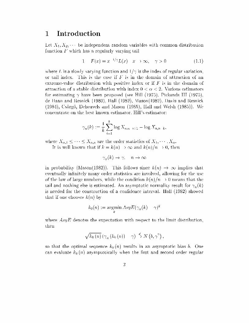
1 Introduction

Let X1; X2; � � � be independent random variables with common distribution

function F which has a regularly varying tail

1� F (x) = x�1= L(x) x!1; > 0 (1.1)

where L is a slowly varying function and 1= is the index of regular variation,

or tail index. This is the case if F is in the domain of attraction of an

extreme-value distribution with positive index or if F is in the domain of

attraction of a stable distribution with index 0 < � < 2. Various estimators

for estimating have been proposed (see Hill (1975), Pickands III (1975),

de Haan and Resnick (1980), Hall (1982), Mason(1982), Davis and Resnick

(1984), Cs�org}o, Deheuvels and Mason (1985), Hall and Welsh (1985)). We

concentrate on the best known estimator, Hill's estimator:

n(k) :=1

k

kXi=1

logXn;n�i+1 � logXn;n�k;

where Xn;1 � � � � � Xn;n are the order statistics of X1; � � � ; Xn.

It is well known that if k = k(n)!1 and k(n)=n! 0, then

n(k)! ; n!1

in probability (Mason(1982)). This follows since k(n) ! 1 implies that

eventually in�nitely many order statistics are involved, allowing for the use

of the law of large numbers, while the condition k(n)=n! 0 means that the

tail and nothing else is estimated. An asymptotic normality result for n(k)

is needed for the construction of a con�dence interval. Hall (1982) showed

that if one chooses k(n) by

k0(n) := argmink

AsyE( n(k)� )2

where AsyE denotes the expectation with respect to the limit distribution,

then pk0 (n) ( n (k0 (n))� )

d! N�b; 2

�;

so that the optimal sequence k0 (n) results in an asymptotic bias b. One

can evaluate k0 (n) asymptotically when the �rst and second order regular

2

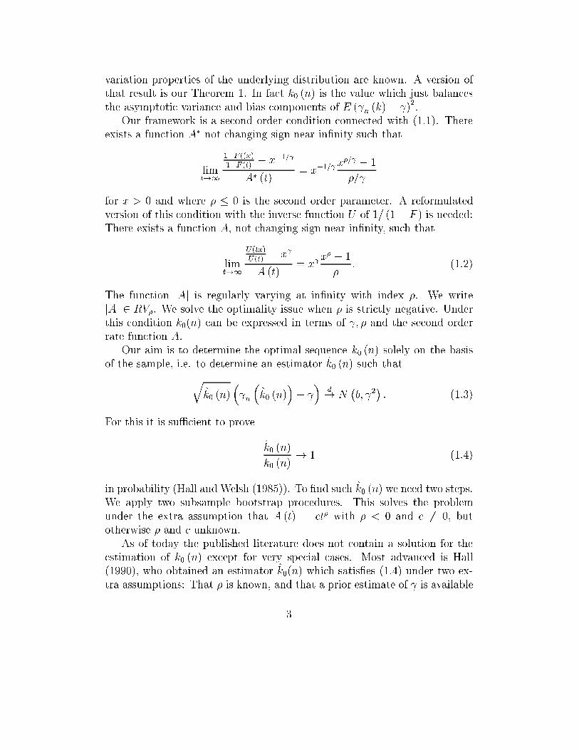
variation properties of the underlying distribution are known. A version of

that result is our Theorem 1. In fact k0 (n) is the value which just balances

the asymptotic variance and bias components of E ( n (k)� )2.

Our framework is a second order condition connected with (1.1). There

exists a function A� not changing sign near in�nity such that

limt!1

1�F ((x)1�F (t)

� x�1=

A� (t)= x�1=

x�= � 1

�=

for x > 0 and where � � 0 is the second order parameter. A reformulated

version of this condition with the inverse function U of 1= (1� F ) is needed:

There exists a function A, not changing sign near in�nity, such that

limt!1

U(tx)U(t)

� x

A (t)= x

x� � 1

�: (1.2)

The function jAj is regularly varying at in�nity with index �. We write

jAj 2 RV�. We solve the optimality issue when � is strictly negative. Under

this condition k0(n) can be expressed in terms of ; � and the second order

rate function A.

Our aim is to determine the optimal sequence k0 (n) solely on the basis

of the sample, i.e. to determine an estimator k̂0 (n) such thatqk̂0 (n)

� n

�k̂0 (n)

�� �

d! N�b; 2

�: (1.3)

For this it is suÆcient to prove

k̂0 (n)

k0 (n)! 1 (1.4)

in probability (Hall and Welsh (1985)). To �nd such k̂0 (n) we need two steps.

We apply two subsample bootstrap procedures. This solves the problem

under the extra assumption that A (t) = ct� with � < 0 and c 6= 0, but

otherwise � and c unknown.

As of today the published literature does not contain a solution for the

estimation of k0 (n) except for very special cases. Most advanced is Hall

(1990), who obtained an estimator k̂0(n) which satis�es (1.4) under two ex-

tra assumptions: That � is known, and that a prior estimate of is available

3

such that this estimator already converges roughly at the optimal rate 1. We

are able to dispense with these assumptions. Nevertheless, Hall's (1990) sug-

gestion to use a bootstrap method was very instrumental for the development

of our automatic and general procedure.

As a byproduct of our approach we obtain a consistent estimator for the

second order parameter �; cf. eq. (3.9) below. We believe this result to be

new to the literature as well.

A completely di�erent approach to the problem is taken in a recent paper

by Drees and Kaufmann (1998). The Drees and Kaufmann method requires

the choice of a tuning parameter. In our case the equivalence of this tuning

parameter is the choice of the bootstrap resample size n1. Below we present

a fully automatic procedure for obtaining n1 in the sense that a heuristic

algorithm is used to determine the bootstrap sample size (see Section 4). An

explicit procedure for choice of the resample size appears to be new to the

literature as well.

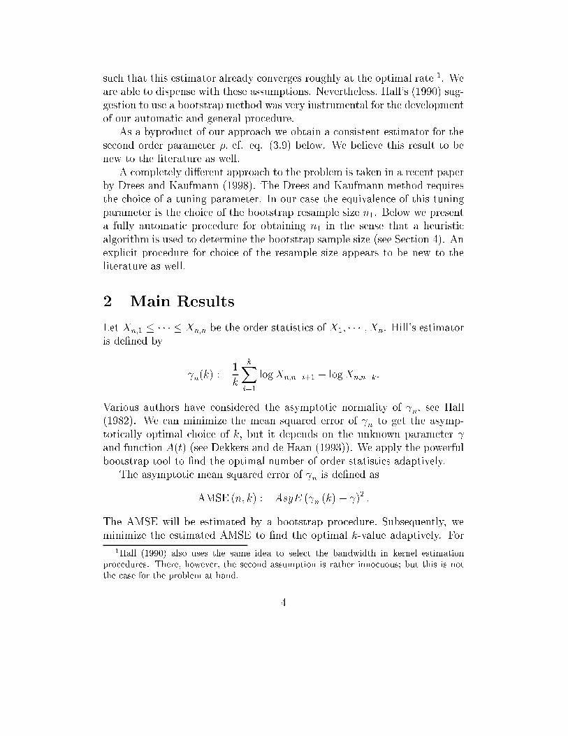
2 Main Results

Let Xn;1 � � � � � Xn;n be the order statistics of X1; � � � ; Xn. Hill's estimator

is de�ned by

n(k) :=1

k

kXi=1

logXn;n�i+1 � logXn;n�k:

Various authors have considered the asymptotic normality of n, see Hall

(1982). We can minimize the mean squared error of n to get the asymp-

totically optimal choice of k, but it depends on the unknown parameter

and function A(t) (see Dekkers and de Haan (1993)). We apply the powerful

bootstrap tool to �nd the optimal number of order statistics adaptively.

The asymptotic mean squared error of n is de�ned as

AMSE (n; k) := AsyE ( n (k)� )2:

The AMSE will be estimated by a bootstrap procedure. Subsequently, we

minimize the estimated AMSE to �nd the optimal k-value adaptively. For

1Hall (1990) also uses the same idea to select the bandwidth in kernel estimation

procedures. There, however, the second assumption is rather innocuous; but this is not

the case for the problem at hand.

4

this to work two problems need to be solved. Even if one were given ,

then the regular bootstrap is not ensured to yield a AMSE estimate which

is asymptotic to AMSE (n; k). Moreover, one does not know in the �rst

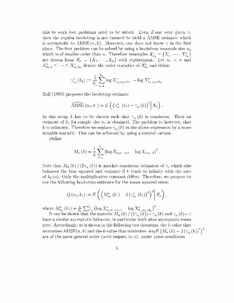
place. The �rst problem can be solved by using a bootstrap resample size n1which is of smaller order than n. Therefore resamples X �

n1= fX�

1 ; � � � ; X�n1g

are drawn from Xn = fX1; � � � ; Xng with replacement. Let n1 < n and

X�n1;1

� � � � � X�n1;n1

denote the order statistics of X �n1

and de�ne

�n1 (k1) :=1

k1

k1Xi=1

logX�n1;n1�i+1 � logX�

n1;n1�k1 :

Hall (1990) proposes the bootstrap estimate

\AMSE (n1; k1) = E�� �n1 (k1)� n (k)

�2���Xn

�:

In this setup k has to be chosen such that n (k) is consistent. Then an

estimate of k1 for sample size n1 is obtained. The problem is, however, that

k is unknown. Therefore we replace n (k) in the above expression by a more

suitable statistic. This can be achieved by using a control variate.

De�ne

Mn (k) =1

k

kXi=1

(logXn;n�i+1 � logXn;n�k)2:

Note that Mn (k) = (2 n (k)) is another consistent estimator of , which also

balances the bias squared and variance if k tends to in�nity with the rate

of k0 (n). Only the multiplicative constant di�ers. Therefore, we propose to

use the following bootstrap estimate for the mean squared error:

Q (n1; k1) := E

��M�

n1(k1)� 2

� �n1 (k1)

�2�2����Xn

�;

where M�n1(k1) =

1k1

Pk1i=1

�logX�

n1;n1�i+1 � logX�n1;n1�k1

�2:

It can be shown that the statisticMn (k) = (2 n (k))� n (k) and n (k)� have a similar asymptotic behavior, in particular both ahve asymptotic mean

zero. Accordingly, as is shown in the following two theorems, the k-value that

minimizes AMSE(n; k) and the k-value that minimizesAsyE�Mn (k)� 2 ( n (k))

2�2

are of the same general order (with respect to n), under some conditions.

5

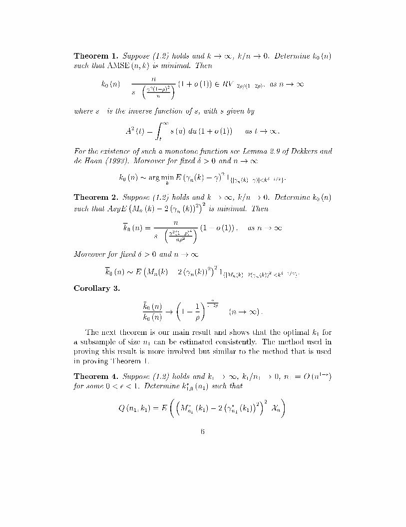
Theorem 1. Suppose (1.2) holds and k ! 1, k=n ! 0. Determine k0 (n)

such that AMSE (n; k) is minimal. Then

k0 (n) =n

s�� 2(1��)2

n

� (1 + o (1)) 2 RV�2�=(1�2�); as n!1

where s� is the inverse function of s, with s given by

A2 (t) =

Z 1

t

s (u) du (1 + o (1)) as t!1:

For the existence of such a monotone function see Lemma 2.9 of Dekkers and

de Haan (1993). Moreover for �xed Æ > 0 and n!1

k0 (n) s argmink

E ( n(k)� )21fj

n(k)� )j<k�1=2g:

Theorem 2. Suppose (1.2) holds and k ! 1, k=n ! 0. Determine �k0 (n)

such that AsyE�Mn (k)� 2 ( n (k))

2�2

is minimal. Then

k0 (n) =n

s�� 2(1��)4

n�2

� (1 + o (1)) ; as n!1

Moreover for �xed Æ > 0 and n!1

k0 (n) s E�Mn(k)� 2 ( n(k))

2�21fjMn(k)�2( n(k))

2j<k�1=2g:

Corollary 3.

�k0 (n)

k0 (n)!�1�

1

�

� 21�2�

(n!1) :

The next theorem is our main result and shows that the optimal k1 for

a subsample of size n1 can be estimated consistently. The method used in

proving this result is more involved but similar to the method that is used

in proving Theorem 1.

Theorem 4. Suppose (1.2) holds and k1 ! 1, k1=n1 ! 0, n1 = O (n1��)

for some 0 < � < 1. Determine k�1;0 (n1) such that

Q (n1; k1) = E

��M�

n1(k1)� 2

� �n1 (k1)

�2�2����Xn

�

6

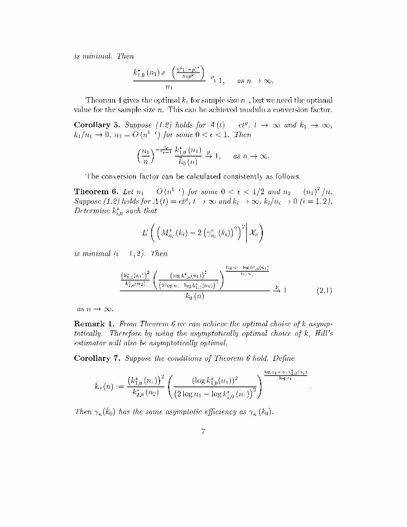
is minimal. Then

k�1;0 (n1) s�� 2(1��)4

n1�2

�n1

p! 1; as n!1:

Theorem 4 gives the optimal k1 for sample size n1, but we need the optimal

value for the sample size n. This can be achieved modulo a conversion factor.

Corollary 5. Suppose (1.2) holds for A (t) = ct�, t ! 1 and k1 ! 1,

k1=n1 ! 0, n1 = O (n1��) for some 0 < � < 1. Then

�n1n

�� 2�2��1 k

�1;0 (n1)

�k0 (n)

p! 1; as n!1:

The conversion factor can be calculated consistently as follows.

Theorem 6. Let n1 = O (n1��) for some 0 < � < 1=2 and n2 = (n1)2=n.

Suppose (1.2) holds for A (t) = ct�, t!1 and ki !1, ki=ni ! 0 (i = 1; 2).

Determine k�i;0 such that

E

��M�

ni(ki)� 2

� �ni (ki)

�2�2����Xn

�

is minimal (i = 1; 2). Then

(k�1;0(n1))2

k�2;0(n2)

�(log k�1;0(n1))

2

(2 log n1�log k�1;0(n1))2

� log n1�log k�1;0(n1)

log n1

k0 (n)

p! 1 (2.1)

as n!1:

Remark 1. From Theorem 6 we can achieve the optimal choice of k asymp-

totically. Therefore by using the asymptotically optimal choice of k, Hill's

estimator will also be asymptotically optimal.

Corollary 7. Suppose the conditions of Theorem 6 hold. De�ne

k̂0 (n) :=

�k�1;0 (n1)

�2k�2;0 (n2)

(log k�1;0(n1))

2�2 logn1 � log k�1;0 (n1)

�2! log n1�log k�1;0(n1)

log n1

:

Then n(k̂0) has the same asymptotic eÆciency as n (k0).

7

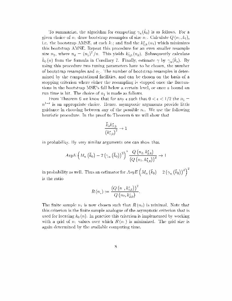
To summarize, the algorithm for computing n(k̂0) is as follows. For a

given choice of n1 draw bootstrap resamples of size n1. Calculate Q (n1; k1),

i.e. the bootstrap AMSE; at each k1; and �nd the k�1;0 (n1) which minimizes

this bootstrap AMSE. Repeat this procedure for an even smaller resample

size n2, where n2 = (n1)2=n. This yields k�2;0 (n2). Subsequently calculate

k̂0 (n) from the formula in Corollary 7. Finally, estimate by n(k̂o). By

using this procedure two tuning parameters have to be chosen, the number

of bootstrap resamples and n1. The number of bootstrap resamples is deter-

mined by the computational facilities, and can be chosen on the basis of a

stopping criterion where either the resampling is stopped once the uctua-

tions in the bootstrap MSE's fall below a certain level, or once a bound on

run time is hit. The choice of n1 is made as follows.

From Theorem 6 we know that for any � such that 0 < � < 1=2 the n1 =

n1�� is an appropriate choice. Hence, asymptotic arguments provide little

guidance in choosing between any of the possible n1. We use the following

heuristic procedure. In the proof to Theorem 6 we will show that

�kok�2;0�

k�1;0�2 ! 1

in probability. By very similar arguments one can show that

AsyE�Mn

��k0�� 2

� n��k0��2�2 Q

�n2; k

�2;0

��Q�n1; k

�1;0

��2 ! 1

in probability as well. Thus an estimator for AsyE�Mn

��k0�� 2

� n��k0��2�2

is the ratio

R (n1) :=

�Q�n1; k

�1;0

��2Q�n2; k

�2;0

� :

The �nite sample n1 is now chosen such that R (n1) is minimal. Note that

this criterion is the �nite sample analogue of the asymptotic criterion that is

used for locating �k0 (n). In practice this criterion is implemented by working

with a grid of n1 values over which R (n1) is minimized. The grid size is

again determined by the available computing time.

8

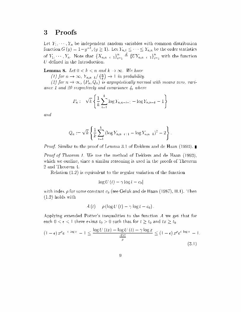
3 Proofs

Let Y1; � � � ; Yn be independent random variables with common distribution

function G (y) = 1�y�1; (y � 1). Let Yn;1 � � � � � Yn;n be the order statistics

of Y1; � � � ; Yn. Note that fXn;n�i+1gni=1

d= fUYn;n�i+1gni=1

with the function

U de�ned in the Introduction.

Lemma 8. Let 0 < k < n and k !1. We have

(1) for n!1, Yn;n�k=�nk

�! 1 in probability.

(2) for n!1, (Pn; Qn) is asymptotically normal with means zero, vari-

ance 1 and 20 respectively and covariance 4, where

Pn :=pk

(1

k

kXi=1

logYn;n�i+1 � logYn;n�k � 1

)

and

Qn :=pk

(1

k

kXi=1

(logYn;n�i+1 � logYn;n�k)2 � 2

):

Proof. Similar to the proof of Lemma 3.1 of Dekkers and de Haan (1993).

Proof of Theorem 1. We use the method of Dekkers and de Haan (1993),

which we outline, since a similar reasoning is used in the proofs of Theorem

2 and Theorem 4.

Relation (1.2) is equivalent to the regular variation of the function

jlogU (t)� log t� c0j

with index � for some constant c0 (see Geluk and de Haan (1987), II.1). Then

(1.2) holds with

A (t) = � (logU (t)� log t� c0) :

Applying extended Potter's inequalities to the function A we get that for

each 0 < � < 1 there exists t0 > 0 such that for t � t0 and tx � t0

(1� �)x�e��j log xj � 1 �logU (tx)� logU (t)� log x

A(t)�

� (1 + �) x�e�j log xj � 1:

(3.1)

9

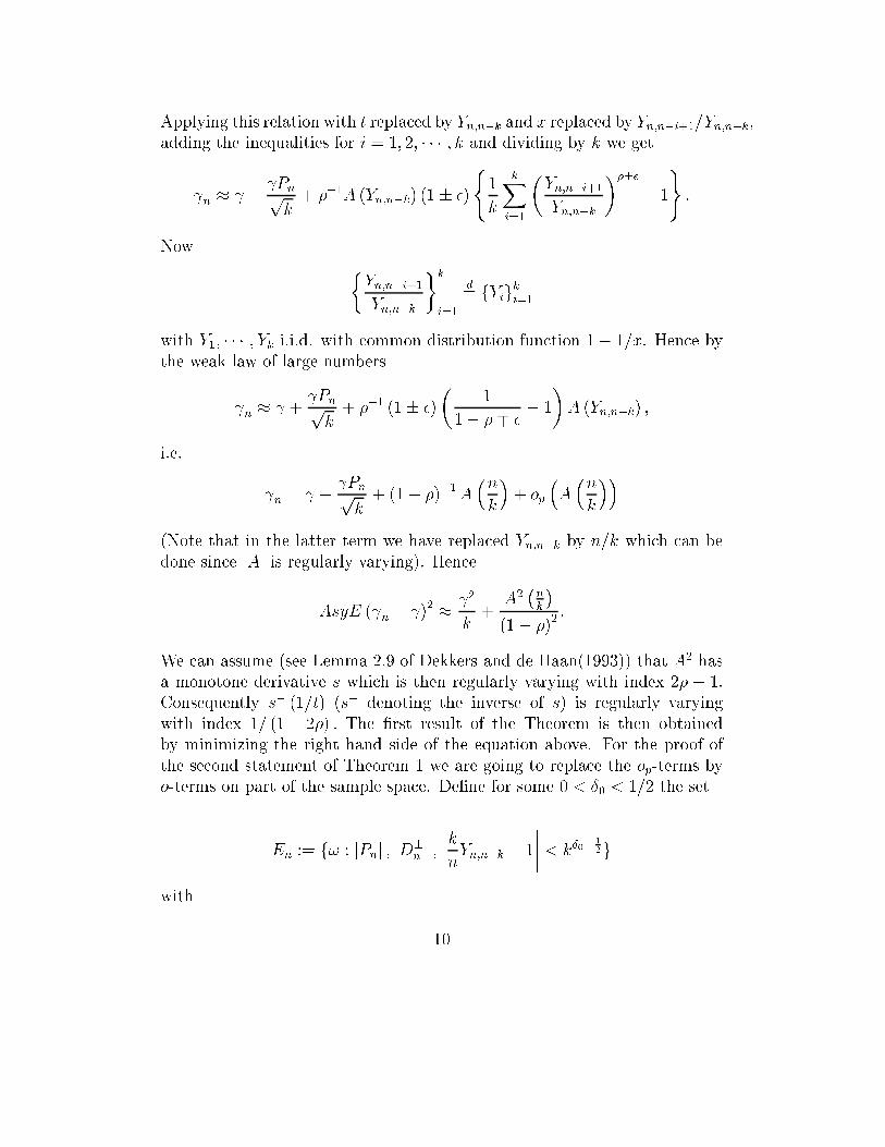
Applying this relation with t replaced by Yn;n�k and x replaced by Yn;n�i+1=Yn;n�k,

adding the inequalities for i = 1; 2; � � � ; k and dividing by k we get

n � + Pnpk+ ��1A (Yn;n�k) (1� �)

(1

k

kXi=1

�Yn;n�i+1

Yn;n�k

����

� 1

):

Now �Yn;n�i+1

Yn;n�k

�k

i=1

d= fYig

ki=1

with Y1; � � � ; Yk i.i.d. with common distribution function 1� 1=x. Hence by

the weak law of large numbers

n � + Pnpk+ ��1 (1� �)

�1

1� �� �� 1

�A (Yn;n�k) ;

i.e.

n = + Pnpk+ (1� �)

�1A�nk

�+ op

�A�nk

��

(Note that in the latter term we have replaced Yn;n�k by n=k which can be

done since jAj is regularly varying). Hence

AsyE ( n � )2 �

2

k+

A2�nk

�(1� �)

2:

We can assume (see Lemma 2.9 of Dekkers and de Haan(1993)) that A2 has

a monotone derivative s which is then regularly varying with index 2� � 1:

Consequently s� (1=t) (s� denoting the inverse of s) is regularly varying

with index 1= (1� 2�) : The �rst result of the Theorem is then obtained

by minimizing the right hand side of the equation above. For the proof of

the second statement of Theorem 1 we are going to replace the op-terms by

o-terms on part of the sample space. De�ne for some 0 < Æ0 < 1=2 the set

En := f! : jPnj ;��D�

n

�� ; ����knYn;n�k � 1

���� < kÆ0�12g

with

10

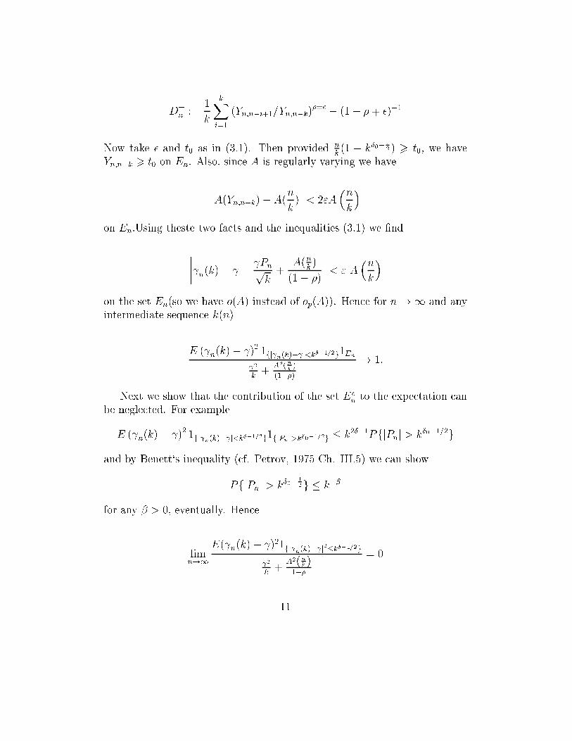
D�n :=

1

k

kXi=1

(Yn;n�i+1=Yn;n�k)��� � (1� �� �)�1

Now take � and t0 as in (3.1). Then provided nk(1 � kÆ0�

12 ) > t0, we have

Yn;n�k > t0 on En. Also, since A is regularly varying we have

���A(Yn;n�k)� A(n

k)��� < 2"A

�nk

�on En:Using theste two facts and the inequalities (3.1) we �nd

���� n(k)� � Pnpk+

A(nk)

(1� �)

���� < " A�nk

�

on the set En(so we have o(A) instead of op(A)). Hence for n!1 and any

intermediate sequence k(n)

E ( n(k)� )21fj n(k)� j<k�1=2g1En

2

k+

A2(nk)

(1��)

! 1:

Next we show that the contribution of the set Ecn to the expectation can

be neglected. For example

E ( n(k)� )21fj n(k)� j<kÆ�1=2g1fjPnj>kÆ0�1=2g � k2Æ�1PfjPnj > kÆ0�1=2g

and by Benett`s inequality (cf. Petrov, 1975 Ch. III.5) we can show

PfjPnj > kÆ0�12g � k��

for any � > 0; eventually. Hence

limn!1

E( n(k)� )21fj n(k)� j2�k�1=2g

2

k+

A2(nk)

1��

= 0

11

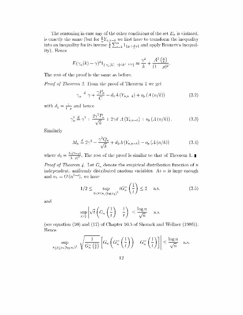
The reasoning in case any of the other conditions of the set En is violated,

is exactly the same (but for knYn;n�k we �rst have to transform the inequality

into an inequality for its inverse 1k

Pni=1 1fyi>n

kxg and apply Bennett`s inequal-

ity). Hence

E( n(k)� )21fj n(k)� j�k�1=2g t 2

k+

A2�nk

�(1� �)2

:

The rest of the proof is the same as before.

Proof of Theorem 2. From the proof of Theorem 1 we get

nd= +

Pn

C+ d1A (Yn;n�k) + op (A (n=k)) (3.2)

with d1 =1

1�� and hence

2nd= 2 +

2 2Pnpk

+ 2 d1A (Yn;n�k) + op (A (n=k)) : (3.3)

Similarly

Mnd= 2 2 +

2Qnpk

+ d2A (Yn;n�k) + op (A (n=k)) (3.4)

where d2 =2 (2��)(1��)2

: The rest of the proof is similar to that of Theorem 1.

Proof of Theorem 4. Let Gn denote the empirical distribution function of n

independent, uniformly distributed random variables. As n is large enough

and n1 = O (n1��), we have

1=2 � sup0<t�n1(log n1)2

tG�n

�1

t

�� 2 a.s. (3.5)

and

supt�2

����pt�Gn

�1

t

��

1

t

����� � lognpn

a.s.

(see equation (10) and (17) of Chapter 10.5 of Shorack and Wellner (1986)).

Hence

sup4�t�n1(log n1)2

�����s

1

G�n

�1t

� �Gn

�G�n

�1

t

���G�

n

�1

t

������� � lognpn

a.s.

12

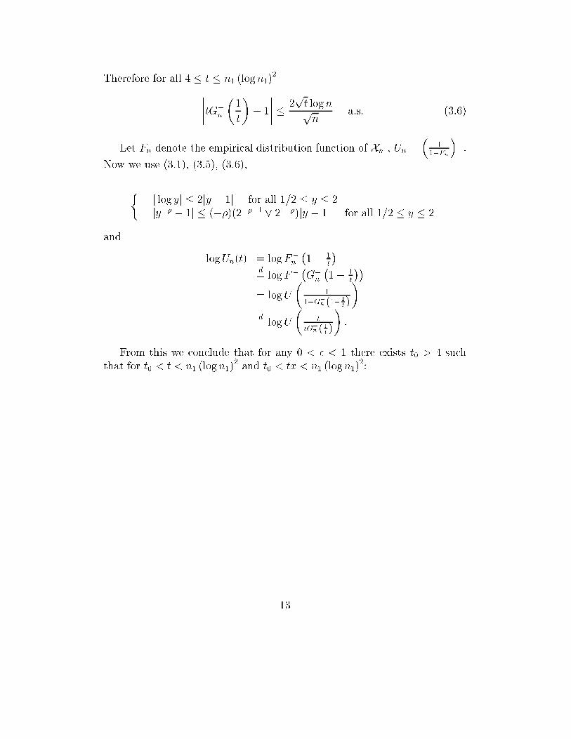
Therefore for all 4 � t � n1 (logn1)2

����tG�n

�1

t

�� 1

���� � 2pt lognpn

a.s. (3.6)

Let Fn denote the empirical distribution function of Xn , Un =�

11�Fn

��.

Now we use (3.1), (3.5), (3.6),

�j log yj � 2jy � 1j for all 1=2 � y � 2

jy�� � 1j � (��)(2���1 _ 21+�)jy � 1j for all 1=2 � y � 2

and

logUn(t) = logF�n

�1� 1

t

�d= logF�

�G�n

�1� 1

t

��= logU

�1

1�G�n (1� 1t)

�d= logU

�t

tG�n ( 1t)

�:

From this we conclude that for any 0 < � < 1 there exists t0 > 4 such

that for t0 < t < n1 (logn1)2and t0 < tx < n1 (logn1)

2:

13

logUn(tx)�logUn(t)� log xA(tx)

�

d=

logU

tx

txG�

n ( 1tx)

!�logU(tx)� log

1

txG�

n ( 1tx)

!

A(tx)

�

A(tx)A(t)

�logU

t

tG�

n ( 1t )

!�logU(t)� log

1

tG�

n ( 1t )

!

A(t)=�+

logU(tx)�logU(t)� log xA(t)=�

+

log

1

txG�

n ( 1tx)

!

A(t)=��

log

1

tG�

n ( 1t )

!

A(t)=�

�h(1 + �)

�txG�

n

�1tx

����e�jlog(txG

�

n ( 1tx))j � 1

i(1 + �) x�e�j log xj

� (1� �)�tG�

n

�1t

����e��jlog(tG

�

n ( 1t))j + 1 + (1 + �)x�e�j log xj � 1

+��� �A(t)

��� 2 ���txG�n

�1tx

�� 1��+ ��tG�

n

�1t

�� 1��� a.s.

� (1 + �)h�txG�

n

�1tx

���� � 1ie�jlog(txG

�

n ( 1tx))j (1 + �) x�e�j log xj

+(1 + �)���e�jlog(txG�n ( 1

tx))j � 1

��� (1 + �) x�e�j log xj

+� (1 + �) x�e�j log xj � (1� �)h�tG�

n

�1t

���� � 1ie��jlog(tG

�

n ( 1t))j

� (1� �)he��jlog(tG

�

n ( 1t))j � 1

i� �

+(1 + �) x�e�j log xj � 1 +��� �A(t)

��� 4pt log npn

(px + 1) a.s.

� (1 + �) (��) (2���1 _ 21+�)��txG�

n

�1tx

�� 1�� e� log 2 (1 + �)x�e�j log xj

+4�e� log 2 (1 + �) x�e�j log xj + (1 + �)2x�e�j log xj � 1

+ (1� �) (��) (2���1 _ 21+�)��tG�

n

�1t

�� 1�� e� log 2

+4� (1� �) e� log 2 � �+��� �A(t)

��� 4pt log npn

(px + 1) a.s.

�h(��) (2��+1 _ 23+�) + 2

��� �A(t)

���i 2pt log npn

(px+ 1)

+ (1 + 9�) (1 + �)x�e�j log xj � 1 + 7� a.s.

(3.7)

14

Similarly

logUn(tx)�logUn(t)� log xA(t)=�

� �h(��) (2��+1 _ 23+�) + 2

��� �A(t)

���i 2pt log npn

(px + 1)

+(1� 9�)(1� �)x�e��j log xj � 1� 7� a.s.

(3.8)

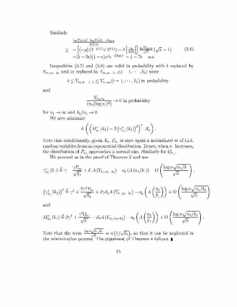
Inequalities (3.7) and (3.8) are valid in probability with t replaced by

Yn1;n1�k1 and tx replaced by Yn1;n1�i+1(i = 1; � � � ; k1) since

4 � Yn1;n1�i+1 � Yn1;n1(i = 1; � � � ; k1) in probability

and

Yn1;n1(n1(logn1)2)

! 0 in probability

for n1 !1 and k1=n1 ! 0.

We now minimize

E

��M�

n1(k1)� 2

� �n1 (k1)

�2�2����Xn

�:

Note that conditionally, given Xn, Pn1 is once again a normalized m of i.i.d.

random variables from an exponential distribution. Hence, when n1 increases,

the distribution of Pn1 approaches a normal one. Similarly for Qn1.

We proceed as in the proof of Theorem 2 and use

�n1 (k1)d= +

Pn1pk1

+ d1A (Yn1;n1�k1) + op (A (n1=k1)) +O

logn

pn1=k1pn

!;

� �n1 (k1)

�2 d= 2 +

2 2Pn1pk1

+ 2 d1A (Yn1;n1�k1) + op

�A

�n1

k1

��+O

logn

pn1=k1pn

!

and

M�n1(k1)

d= 2 2 +

2Qn1pk1

+ d2A (Yn1;n1�k1) + op

�A

�n1

k1

��+O

logn

pn1=k1pn

!:

Note that the termlog n

pn1=k1pn

= o�1=pk1�, so that it can be neglected in

the minimization process. The statement of Theorem 4 follows.

15

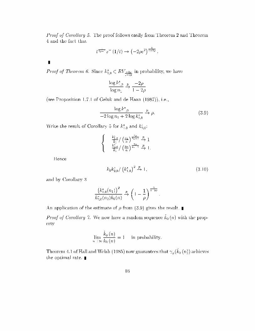
Proof of Corollary 5. The proof follows easily from Theorem 2 and Theorem

4 and the fact that

t1

2��1 s� (1=t)!��2�c2

� 11�2� :

Proof of Theorem 6. Since k�1;0 2 RV �2�

1�2�in probability, we have

log k�1;0

logn1

p!�2�1� 2�

(see Proposition 1.7.1 of Geluk and de Haan (1987)), i.e.,

log k�1;0

�2 logn1 + 2 log k�1;0

p! �: (3.9)

Write the result of Corollary 5 for k�1;0 and k�2;0:8<:

k�1;0�k0=�n1n

� 2�

2��1p! 1

k�2;0�k0=�n2n

� 2�2��1

p! 1:

Hence

�k0k�2;0=

�k�1;0�2 p! 1; (3.10)

and by Corollary 3 �k�1;0(n1)

�2k�2;0(n2)k0(n)

p!�1�

1

�

� 21�2�

:

An application of the estimate of � from (3.9) gives the result.

Proof of Corollary 7. We now have a random sequence k̂0 (n) with the prop-

erty

limn!1

k̂0 (n)

k0 (n)= 1 in probability:

Theorem 4.1 of Hall andWelsh (1985) now guarantees that n(k̂0 (n)) achieves

the optimal rate.

16

4 Simulation and Estimation

We investigate the performance of our fully automatic estimation procedure

by means of Monte Carlo experiments and by an application to some �nancial

data sets, i.e. the stock price index S&P-500 and foreign exchange quote

data. The sample sizes are typical for current �nancial data sets, ranging

from 2,000 to 20,000 observations. The sample sizes in the Monte Carlo

experiments were chosen to be equally large.

4.1 Simulations

We evaluate the performance of our estimators for , � and k0 (n) on the basis

of pseudo i.i.d. random numbers from the Student-t and type II extreme

value distributions in addition to two cases of dependent data. The tail

index 1= equals the degrees of freedom in case of the Student-t distribution.

Recall that the type II extreme value distribution reads exp��x�1=

�: We

focus on 1= = 1; 4 and 11. For the Student-t distribution �= = �2, whilefor the extreme value distribution � = �1.

In addition to the i.i.d. data, we also investigate the performance of

our estimator for dependent data. From Hsing (1991), Resnick and Starica

(1998), and Embrechts et al. (1997) we know that the Hill estimator is consis-

tent for dependent data like ARMA processes and ARCH-type processes. We

focus on two stochastic processes. First, the MA(1) process Yt = Xt +Xt�1;

where the Xt are i.i.d. Student-t with 1= = 3 degrees of freedom is consid-

ered. The �rst and second order parameters of the tail expansion of Yt can be

computed by standard calculus methods. The interest in this process derives

from the fact that while n (k) is biased upwards for Student-t distributions,

the bias switches sign for the marginal distribution of Y; i.e. the c-parameter

in the A (t) function switches sign.

The other stochastic process exhibits conditional heteroscedasticity. Fi-

nancial time series return data typically have the fair game property with

dependence only in the second moment, see e.g. Bollerslev, Chou and Kro-

ner (1992) and Embrechts, Kluppelberg and Mikosch (1997). The following

process, denoted as Stochastic Volatility, is typical for the processes that are

17

used to model �nancial return data:

Yt = UtXtHt;

Ut � i.i.d. discrete uniform on � 1; 1;

Xt =p57=Zt; Zt � �(3) i.i.d. ;

Ht = 0:1Qt + 0:9Ht�1; Qt � N (0; 1) ; i.i.d.

The Xt and Zt are chosen such that the marginal distribution of Yt has a

Student-t with 3 degrees of freedom distribution. This allows us to evaluate

the performance of our procedure.

The results of the Monte Carlo experiments are reported in Table 1 and

Table 2 for sample sizes of 2,000 and 20,000 respectively. Each table is based

on 250 simulations per distribution. For the choice of the tuning parameter n1we use the procedure described at the end of section 2. Hence, for n = 2; 000

we searched over the interval from n1 = 600 to n1 = 1; 700 by increments

of 100. The number of bootstrap resamples was 1,000. In the larger sample

with size n = 20; 000 we searched from n1 = 2; 000 to n1 = 15; 000, with

increments of 1,000, using 500 bootstrap resamples for each n1. The grid size

could be made much �ner, and the number of resamples larger for a speci�c

data set in order to increase the precision. For each distribution we report

the true value of the parameter, the mean, the standard error (s.e.) and the

root mean squared error (RMSE). We report estimates for and ��, whilek̂0 (n) is reported relative to k0 (n).

From the Tables 1 and 2 we see that the estimator for the inverse tail index

performs well in terms of bias and standard error for both the larger and the

smaller sample sizes. Evidently, in most cases are the bias and standard error

lower for the larger sample size n = 20; 000. The only exception to decent

performance in terms of bias is the Student-t with 11 degrees of freedom,

since it is heavily upwards biased in the smaller sample. This occurs even

though the RMSE does not vary that much with for the Student-t class.

Thus for some applications the RMSE criterion may give too low a weight

to the bias. The method also works well for the two stochastic processes.

The estimates for the second order parameter � are less precise than those

for the �rst order parameter (after rescaling the standard error by the true

parameter value). The tail observations are naturally more informative about

the leading terms of the expansion at in�nity. Because k̂0 (n) depends on �̂,

it is not surprising to see that the same observation applies to k̂0 (n) =k0 (n).

As was predicted on the basis of the theoretical parameters, the MA(1) -

18

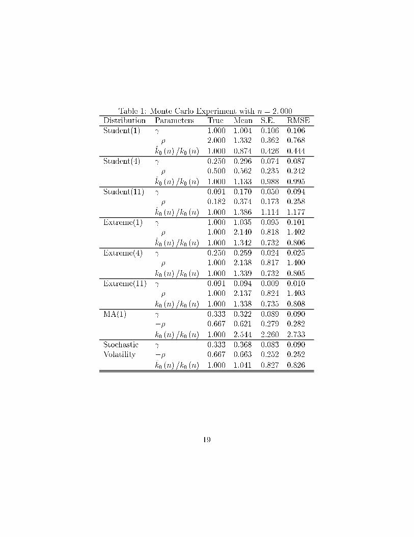
Table 1: Monte Carlo Experiment with n = 2; 000Distribution Parameters True Mean S.E. RMSE

Student(1) 1.000 1.004 0.106 0.106

�� 2.000 1.332 0.362 0.768

k̂0 (n) =k0 (n) 1.000 0.874 0.426 0.444

Student(4) 0.250 0.296 0.074 0.087

�� 0.500 0.562 0.235 0.242

k̂0 (n) =k0 (n) 1.000 1.133 0.988 0.995

Student(11) 0.091 0.170 0.050 0.094

�� 0.182 0.374 0.173 0.258

k̂0 (n) =k0 (n) 1.000 1.386 1.114 1.177

Extreme(1) 1.000 1.035 0.095 0.101

�� 1.000 2.140 0.818 1.402

k̂0 (n) =k0 (n) 1.000 1.342 0.732 0.806

Extreme(4) 0.250 0.259 0.024 0.025

�� 1.000 2.138 0.817 1.400

k̂0 (n) =k0 (n) 1.000 1.339 0.732 0.805

Extreme(11) 0.091 0.094 0.009 0.010

�� 1.000 2.137 0.824 1.403

k̂0 (n) =k0 (n) 1.000 1.338 0.735 0.808

MA(1) 0.333 0.322 0.089 0.090

�� 0.667 0.621 0.279 0.282

k̂0 (n) =k0 (n) 1.000 2.544 2.260 2.733

Stochastic 0.333 0.368 0.083 0.090

Volatility �� 0.667 0.663 0.252 0.252

k̂0 (n) =k0 (n) 1.000 1.041 0.827 0.826

19

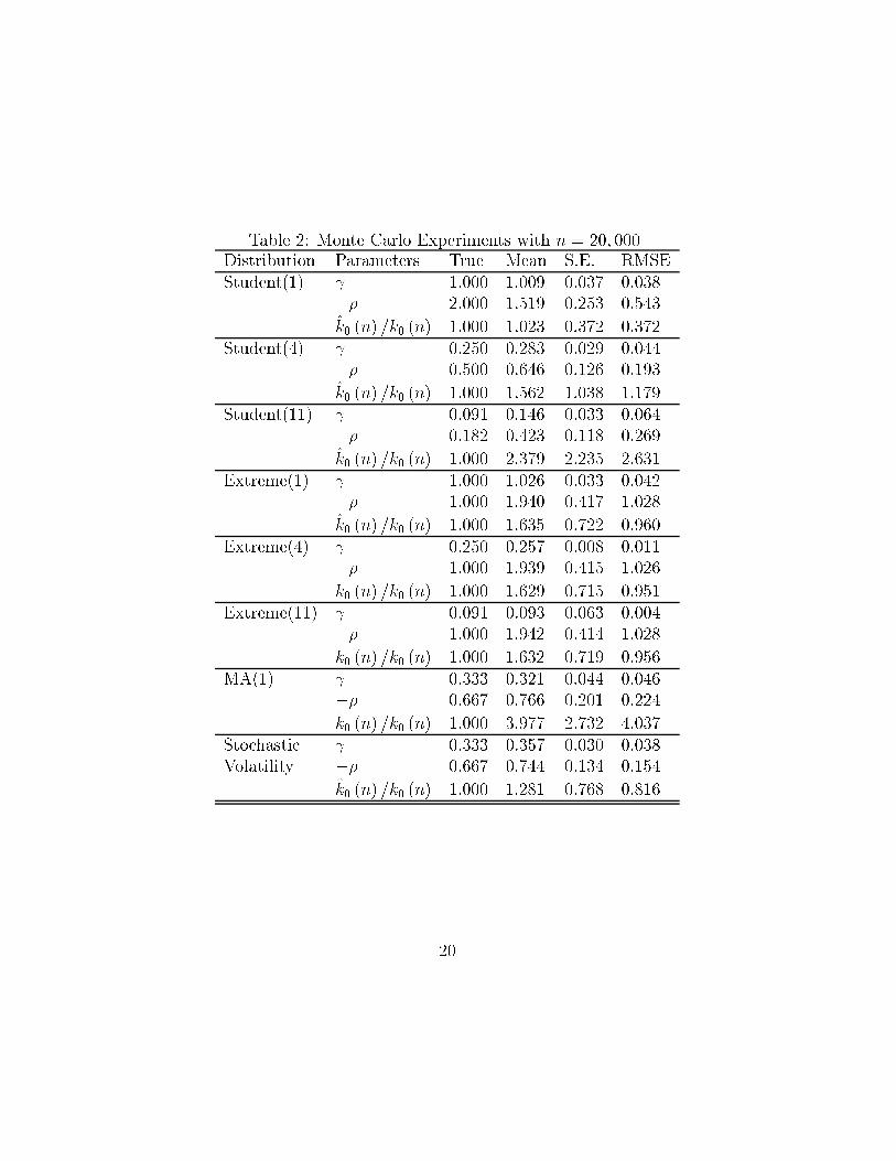
Table 2: Monte Carlo Experiments with n = 20; 000Distribution Parameters True Mean S.E. RMSE

Student(1) 1.000 1.009 0.037 0.038

�� 2.000 1.519 0.253 0.543

k̂0 (n) =k0 (n) 1.000 1.023 0.372 0.372

Student(4) 0.250 0.283 0.029 0.044

�� 0.500 0.646 0.126 0.193

k̂0 (n) =k0 (n) 1.000 1.562 1.038 1.179

Student(11) 0.091 0.146 0.033 0.064

�� 0.182 0.423 0.118 0.269

k̂0 (n) =k0 (n) 1.000 2.379 2.235 2.631

Extreme(1) 1.000 1.026 0.033 0.042

�� 1.000 1.940 0.417 1.028

k̂0 (n) =k0 (n) 1.000 1.635 0.722 0.960

Extreme(4) 0.250 0.257 0.008 0.011

�� 1.000 1.939 0.415 1.026

k̂0 (n) =k0 (n) 1.000 1.629 0.715 0.951

Extreme(11) 0.091 0.093 0.063 0.004

�� 1.000 1.942 0.414 1.028

k̂0 (n) =k0 (n) 1.000 1.632 0.719 0.956

MA(1) 0.333 0.321 0.044 0.046

�� 0.667 0.766 0.201 0.224

k̂0 (n) =k0 (n) 1.000 3.977 2.732 4.037

Stochastic 0.333 0.357 0.030 0.038

Volatility �� 0.667 0.744 0.134 0.154

k̂0 (n) =k0 (n) 1.000 1.281 0.768 0.816

20

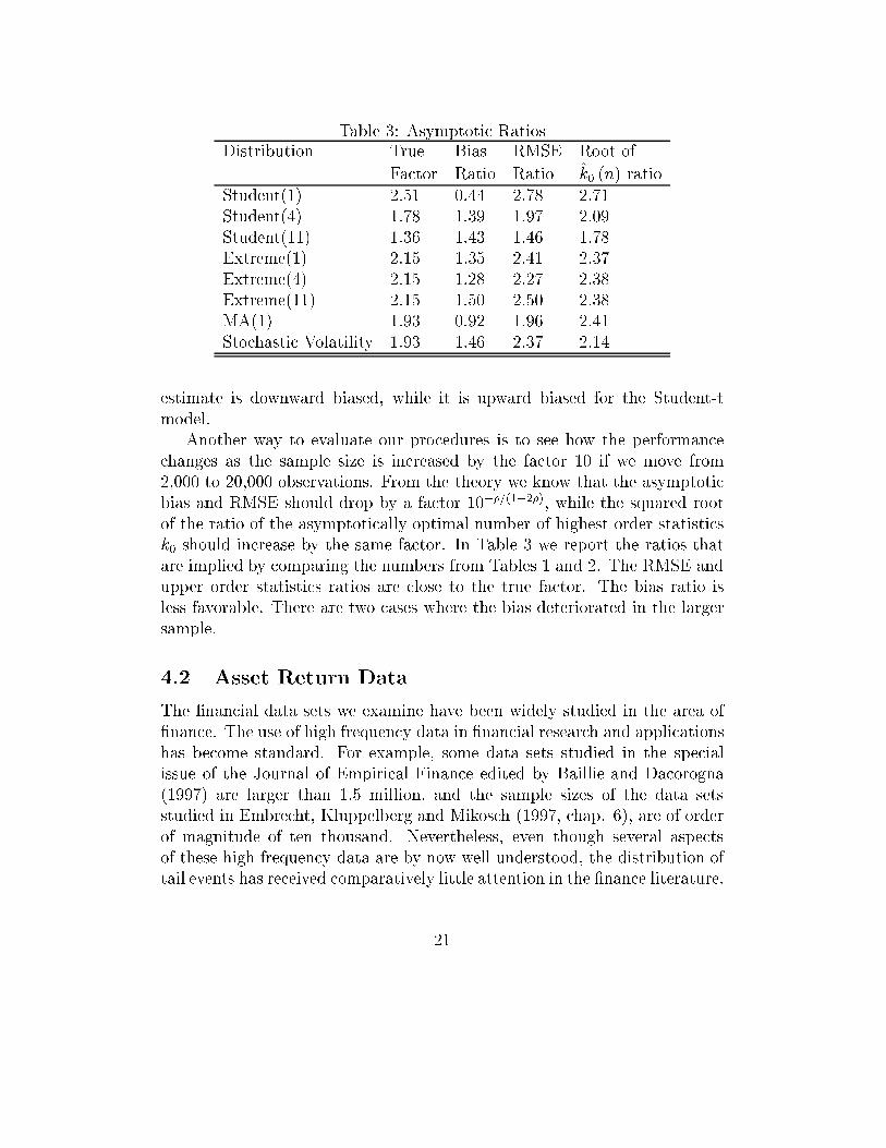
Table 3: Asymptotic RatiosDistribution True Bias RMSE Root of

Factor Ratio Ratio k̂0 (n) ratio

Student(1) 2.51 0.44 2.78 2.71

Student(4) 1.78 1.39 1.97 2.09

Student(11) 1.36 1.43 1.46 1.78

Extreme(1) 2.15 1.35 2.41 2.37

Extreme(4) 2.15 1.28 2.27 2.38

Extreme(11) 2.15 1.50 2.50 2.38

MA(1) 1.93 0.92 1.96 2.41

Stochastic Volatility 1.93 1.46 2.37 2.14

estimate is downward biased, while it is upward biased for the Student-t

model.

Another way to evaluate our procedures is to see how the performance

changes as the sample size is increased by the factor 10 if we move from

2,000 to 20,000 observations. From the theory we know that the asymptotic

bias and RMSE should drop by a factor 10��=(1�2�), while the squared root

of the ratio of the asymptotically optimal number of highest order statistics

k0 should increase by the same factor. In Table 3 we report the ratios that

are implied by comparing the numbers from Tables 1 and 2. The RMSE and

upper order statistics ratios are close to the true factor. The bias ratio is

less favorable. There are two cases where the bias deteriorated in the larger

sample.

4.2 Asset Return Data

The �nancial data sets we examine have been widely studied in the area of

�nance. The use of high frequency data in �nancial research and applications

has become standard. For example, some data sets studied in the special

issue of the Journal of Empirical Finance edited by Baillie and Dacorogna

(1997) are larger than 1,5 million, and the sample sizes of the data sets

studied in Embrecht, Kluppelberg and Mikosch (1997, chap. 6), are of order

of magnitude of ten thousand. Nevertheless, even though several aspects

of these high frequency data are by now well understood, the distribution of

tail events has received comparatively little attention in the �nance literature.

21

On the other hand, this is of clear importance for such applications as risk

management. Here we describe the shape of the tails for two of such data

sets.

We selected daily returns from the S&P 500 stock index with 18,024 ob-

servations from 1928 to 1997, and data extracted from all quotes on the

DM-Dollar contract from September 1992 to October 1993. The quotes data

was supplied by Olsen and Associates who continuously collect these data

from the markets. The number of quotes is over 1,5 million, and these are

irregularly spaced throughout the year. The quotes were aggregated into

52,558 10 minute return observations. The data and the aggregation proce-

dures are described by Danielsson and de Vries (1997). In order to examine

the change in the tail properties of the data over the time interval we de-

cided to create subsamples of the �rst 2,000 and last 2,000 observations for

both data sets in addition to using the �rst and last 20,000 observations on

the foreign exchange rate data, and the entire stock index data set. In the

estimation procedure we employed the same grid for n1 as are used in the

simulations; the number of bootstrap resamples, however, was increased to

5,000.

Let Pt be the price at time t of a �nancial asset like equity or foreign

exchange. The compound return on holding such an asset for one period is

log (Pt+1=Pt) : Hence, returns are denomination free. Therefore returns on

di�erent assets can be directly compared. One dimension along which the

asset returns can be compared in order to assess their relative risk charac-

teristics is by means of the tail index. Financial corporations are required

to use large data sets on past returns to evaluate the risk on their trading

portfolio. The minimum required capital stock of these �nacial institutions

is determined on the basis of this risk. The capital requirement ensures that

banks can meet the incidental heavy losses that are so characteristic for the

�nancial markets. The frequency of these large losses can be analyzed by

means of extreme value theory; see e.g. Jansen and de Vries (1991) for an

early example of this approach, and Embrechts et al. (1997) for a more recent

treatment. In this analysis, the measurement of is very important because

it indicates the shape and heaviness of the distribution of returns. It is the

essential input for predictions of out of sample losses, see de Haan, Jansen,

Koedijk and de Vries (1994).

In Table 4 we report some descriptive statistics. The mean return and

standard error of the returns have been annualized because the magnitude

in the high frequency returns is typically very small (for the daily return

22

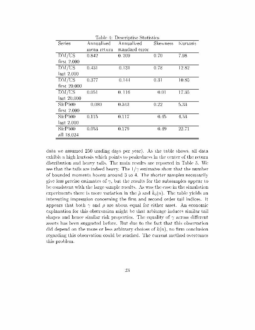
Table 4: Descriptise StatisticsSeries Annualized Annualized Skewness Kurtosis

mean return standard error

DM/US 0:842 0: 209 0:70 7:98

�rst 2,000

DM/US 0:431 0:131 0:78 12:82

last 2,000

DM/US 0:377 0:144 0:31 10:85

�rst 20,000

DM/US 0:051 0: 116 �0:01 17:35

last 20,000

S&P500 �0:080 0:343 0:22 5:33

�rst 2,000

S&P500 0:115 0:117 �0:45 4:53

last 2,000

S&P500 0:053 0:179 �0:49 22:71

all 18,024

data we assumed 250 trading days per year). As the table shows, all data

exhibit a high kurtosis which points to peakedness in the center of the return

distribution and heavy tails. The main results are reported in Table 5. We

see that the tails are indeed heavy. The 1= estimates show that the number

of bounded moments hovers around 3 to 4. The shorter samples necessarily

give less precise estimates of , but the results for the subsamples appear to

be consistent with the large sample results. As was the case in the simulation

experiments there is more variation in the �̂ and k̂0(n). The table yields an

interesting impression concerning the �rst and second order tail indices. It

appears that both and � are about equal for either asset. An economic

explanation for this observation might be that arbitrage induces similar tail

shapes and hence similar risk properties. The equality of across di�erent

assets has been suggested before. But due to the fact that this observation

did depend on the more or less arbitrary choices of k(n), no �rm conclusion

regarding this observation could be reached. The current method overcomes

this problem.

23

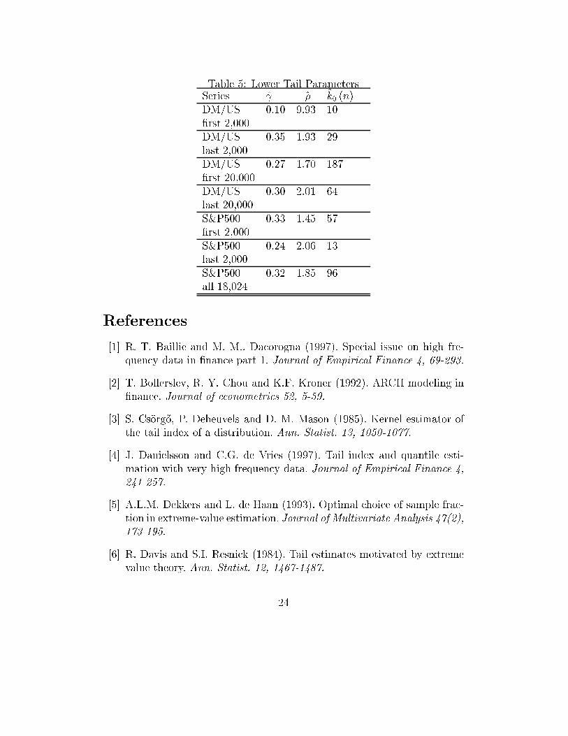
Table 5: Lower Tail ParametersSeries ̂ ��̂ k̂0 (n)

DM/US 0.10 9.93 10

�rst 2,000

DM/US 0.35 1.93 29

last 2,000

DM/US 0.27 1.70 187

�rst 20,000

DM/US 0.30 2.01 64

last 20,000

S&P500 0.33 1.45 57

�rst 2,000

S&P500 0.24 2.06 13

last 2,000

S&P500 0.32 1.85 96

all 18,024

References

[1] R. T. Baillie and M. M.. Dacorogna (1997). Special issue on high fre-

quency data in �nance part 1. Journal of Empirical Finance 4, 69-293.

[2] T. Bollerslev, R. Y. Chou and K.F. Kroner (1992). ARCH modeling in

�nance. Journal of econometrics 52, 5-59.

[3] S. Cs�org}o, P. Deheuvels and D. M. Mason (1985). Kernel estimator of

the tail index of a distribution. Ann. Statist. 13, 1050-1077.

[4] J. Danielsson and C.G. de Vries (1997). Tail index and quantile esti-

mation with very high frequency data. Journal of Empirical Finance 4,

241-257.

[5] A.L.M. Dekkers and L. de Haan (1993). Optimal choice of sample frac-

tion in extreme-value estimation. Journal of Multivariate Analysis 47(2),

173-195.

[6] R. Davis and S.I. Resnick (1984). Tail estimates motivated by extreme

value theory. Ann. Statist. 12, 1467-1487.

24

[7] H. Drees and E. Kaufmann (1998). Selection of the optimal sample frac-

tion in univariate extreme value estimation. Stochastic Process. Appl.

75, 149-172.

[8] P. Embrechts, C. Kuppelberg and T. Mikosch (1997). Modelling Ex-

treme Events. Springer Verlag.

[9] J. Geluk and L. de Haan (1987). Regular Variation, Extensions and

Tauberian Theorems. CWI Tract 40, Amsterdam.

[10] L. de Haan, D.W. Jansen, K. Koedijk and C.G. de Vries (1994). Safety

�rst portfolio selection, extreme value theory and long run asset risks. In

J. Galambos, J. Lechner, E. Simiu and N. Macri (eds.), Extreme Value

Theory and Applications, 471-487.

[11] L. de Haan and S.I. Resnick (1980). A simple asymptotic estimate for

the index of a stable distribution. J. Roy. Statist. Soc. Ser. B 42, 83-87.

[12] P. Hall (1982). On some simple estimates of an exponent of regular

variation. J. Roy. Statist. Soc. B 42, 37-42.

[13] P. Hall (1990). Using the bootstrap to estimate mean squared error

and select smoothing parameter in nonparametric problems. Journal of

Multivariate Analysis 32, 177-203.

[14] P. Hall and A.H. Welsh (1985). Adaptive estimate of parameters of reg-

ular variation. Ann. Statist. 13, 331-341.

[15] B.M. Hill (1975). A simple general approach to inference about the tail

of a distribution. Ann. Statist. 3, 1163-1174.

[16] T. Hsing (1991). On tail index estimation using dependent data. Ann.

of Stat. 19, 1547-1569.

[17] D.W. Jansen and C.G. de Vries (1991). On the frequency of large stock

returns: putting booms and busts into perspective. Review of Economics

and Statistics 73, 18-24.

[18] D.M. Mason (1982). Law of large numbers for sum of extreme values.

Ann. Probab. 10, 754-764

25

[19] V.V. Petrov (1975). Sums of independent random variables, Springer,

New York.

[20] J. Pickands III (1975). Statistical inference using extreme order statis-

tics. Ann. Statist. 3, 119-131.

[21] S. Resnick and C. Starica (1998). Tail index estimation for dependent

data. Ann. Appl. Probab. 8, 1156-1183.

[22] G. Shorack and J. Wellner (1986). Empirical Processes with Applications

to Statistics. John Wiley & Sons.

26