Geostatistical modelling of regional bird species richness: exploring environmental proxies for conservation purpose

ORI GIN AL PA PER

Geostatistical modelling of regional bird species richness:exploring environmental proxies for conservationpurpose

Giovanni Bacaro • Elisa Santi • Duccio Rocchini • Francesco Pezzo •

Luca Puglisi • Alessandro Chiarucci

Received: 13 September 2010 / Accepted: 16 April 2011 / Published online: 27 April 2011� Springer Science+Business Media B.V. 2011

Abstract Identifying spatial patterns in species diversity represents an essential task to be

accounted for when establishing conservation strategies or monitoring programs. Pre-

dicting patterns of species richness by a model-based approach has recently been recog-

nised as a significant component of conservation planning. Finding those environmental

predictors which are related to these patterns is crucial since they may represent surrogates

of biodiversity, indicating in a fast and cheap way the spatial location of biodiversity

hotspots and, consequently, where conservation efforts should be addressed. Predictive

models based on classical multiple linear regression or generalised linear models crowded

the recent ecological literature. However, very often, problems related with spatial auto-

correlation in observed data were not adequately considered. Here, a spatially-explicit

data-set on birds presence and distribution across the whole Tuscany region was analysed.

Species richness was calculated within 1 9 1 km grid cells and 10 environmental pre-

dictors (e.g. altitude, habitat diversity and satellite-derived landscape heterogeneity indi-

ces) were included in the analysis. Integrating spatial components of variation with

predictive ecological factors, i.e. using geostatistical models, a general model of bird

species richness was developed and used to obtain predictive regional maps of bird

G. Bacaro (&) � F. Pezzo � A. ChiarucciBIOCONNET, BIOdiversity and CONservation NETwork, Dipartimento di Scienze Ambientali‘‘G.Sarfatti’’, Universita di Siena, Via P. A. Mattioli 4, 53100 Siena, Italye-mail: [email protected]

E. SantiIRPI-CNR, Via Madonna Alta 126, 06128 Perugia, Italy

G. Bacaro � D. Rocchini � A. ChiarucciTerraData s.r.l. Environmetrics, Dipartimento di Scienze Ambientali‘‘G. Sarfatti’’, Universita di Siena,Via P.A. Mattioli 4, 53100 Siena, Italy

D. RocchiniDepartment of Biodiversity and Molecular Ecology, GIS and Remote Sensing Unit, FondazioneEdmund Mach, Research and Innovation Centre, Via E. Mach 1, 38010 S. Michele all’Adige, TN, Italy

F. Pezzo � L. PuglisiCentro Ornitologico Toscano, C.P. 470, 57100 Livorno, Italy

123

Biodivers Conserv (2011) 20:1677–1694DOI 10.1007/s10531-011-0054-8

diversity hotspots. A meaningful subset of environmental predictors, namely habitat pro-

ductivity, habitat heterogeneity, combined with topographic and geographic information,

were included in the final geostatistical model. Conservation strategies based on the pre-

dicted hotspots as well as directions for increasing sampling effort efficiency could be

extrapolated by the proposed model.

Keywords Bird richness � Conservation � Distribution maps � Natura 2000 network �Predictive model � Semivariance � Spatial autocorrelation � Tuscany � NDVI

Introduction

The identification of spatial patterns in species diversity represents an essential task for

biodiversity conservation strategies or monitoring programs (Cabeza et al. 2004; Pressey

et al. 1993; Williams et al. 1999). Even if geographical patterns of species richness are one of

the central topics in ecology and gained much importance in recent years (e.g. Jetz and

Rahbek 2002; Currie et al. 2004; Field et al. 2005), it is clear that describing spatial patterns of

species using complete censuses of various taxa is difficult, because of the costs associated to

the collection of species distribution data (Williams and Gaston 1994; Palmer et al. 2002;

Baffetta et al. 2007; Rocchini et al. 2009, 2011). Moreover, the quality of data collected at

different sites of interest are likely to contain gaps (Polasky and Solow 2001), which can lead

to erroneous conclusions on the conservation value of a site (Bacaro et al. 2009). To overcome

such limitations, conservation biologists have concentrated their efforts on the development

of effective approaches that would allow accurate predictions of species richness.

Recently, species distribution modeling emerged as a new approach to generate species

distribution maps, on the basis of the relationship between species presence (or abundance)

records and environmental variables (e.g. Araujo and Guisan 2006). The power of the

modeling process depends on the selection of appropriate predictors (Austin 2002; Austin

et al. 2006) and the choice of an adequate spatial scale where inference about the examined

response variable is to be performed (Pearson and Carroll 1999). Grain and extent play a

crucial role and their effects on the statistical results could affect the conclusions about

patterns and processes in models (Dalthorp 2004; Csontos et al. 2007).

Typically, modeling methods attempt to predict the probability of occurrence of (or

environmental suitability for) species as a function of a set of selected environmental

variables. In particular, geostatistical modeling techniques, which have been developed

mainly in the field of geography, are designed to model spatially dependent observations

(Matheron 1963; Krige 1966; Cressie 1990; Goovaerts 1997), but in recent years, such

methodologies have been applied even in the ecological literature (Legendre 1993; Cooper

et al. 1997; Carroll and Pearson 1998; Bacaro and Ricotta 2007, 2009).

Birds are among the best-studied organisms, especially in Europe. They are often

considered as excellent indicators of environmental changes (Gregory et al. 2004; Bani

et al. 2006) and as good ecological proxies to assess the biodiversity values of an area, even

for other taxa which are difficult to sample (Prendergast et al. 1993; Kati et al. 2004;

Maccherini et al. 2009, Santi et al. 2010). Local distribution patterns of birds assemblages

might be a function of the configuration and composition of the vegetation (e.g. Cody

1985; Block and Brennan 1993). Several studies investigated the links between bird spe-

cies diversity and habitat diversity. In general, it was observed that the diversity of bird

species increases with the structural complexity of the vegetation (e.g. MacArthur et al.

1966; Barbaro et al. 2006; Kark et al. 2007; Bino et al. 2008). Moreover measures of

1678 Biodivers Conserv (2011) 20:1677–1694

123

topography or topoclimate have also been shown to be effective explanatory and predictive

variables of species richness in bird communities (e.g. Scott et al. 2002; Thomson et al.

2007).

In this article, a geostatistical modelling approach was applied on the data provided by

the ‘‘Monitoring Program of Breeding Birds of Tuscany’’, one of the most extensive

regional bird monitoring programs in Italy. The aim of this article is twofold: (i) to describe

the spatial patterns of bird species richness and (ii) to identify those environmental factors

underlying these patterns. This latter point represents an important task in the ecological

context since the environmental proxies driving bird richness could be used to decide

conservation strategies.

Methods

Study area and bird data

Tuscany (k 9–12� E, / 42–44� N) covers an area of 22,990 km2 and has extremely het-

erogeneous morphological and land cover features. A great contrast in altitude, a complex

relief and other geographic factors promote climate diversity: the climate ranges from

Mediterranean to temperate, according to the altitudinal and geographical gradients and the

distance from the sea (Raspetti and Vittorini 1995). The majority of the territory is

comprised between an elevation of 0 and 600 m, but in the Apennines the elevation exceed

2,000 m (max elevation 2,054 m).

According to the CORINE Land Cover Map (see Bossard et al. 2000), the dominant

land cover types are represented by cultivated lands (about 45% of the area), and forests

(44%), with natural grasslands and shrublands (6%) and urban artificial areas (4%) cov-

ering most of the remaining area. Forests are mostly placed in the hilly and mountainous

areas. The dominant forest species are oaks (Quercus ilex, Quercus pubescens, Quercuscerris), Mediterranean pines (Pinus pinaster, Pinus pinea), chestnut (Castanea sativa),

beech (Fagus sylvatica) and spruce (Abies alba).

The bird species occurrence data were obtained from the Monitoring Program of

Breeding Birds of Tuscany carried out by the Centro Ornitologico Toscano

(www.centrornitologicotoscano.org) and based on Point Counts method (Bibby et al.2000). Points were distributed according to a two stages sampling design: in randomly

selected 10 9 10 km UTM cells, a number of 12–15 point counts were selected according

to a second random sampling procedure. From a formal point of view, each observation

represents a sample point in space. The used sample design ensured the homogeneous

distribution of observational points across the whole regional surface.

The geo-referenced points (observations) of species occurrences collected in the period

2000–2006 were used in this article. The original data set of geo-referenced observations

was assembled to produce a regional map of bird species richness for cells of 1 9 1 km.

The 1 9 1 km resolution was chosen in order to be consistent with other European cen-

suses (e.g. Koellner et al. 2004; Wohlgemuth et al. 2008). Such a grid covering the whole

Tuscany region resulted in 22,060 cells (Table 1), 3,584 of which enclosed data on bird

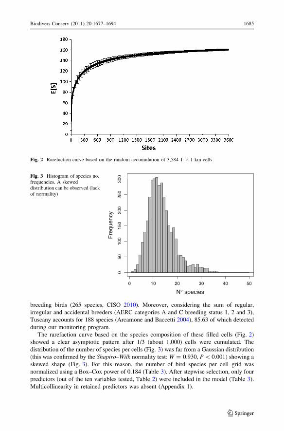
occurrences (Fig. 1). A sample-based rarefaction curve (Gotelli and Colwell 2001) was

calculated to describe the adequacy of the sampling effort. The analytical formula

(Kobayashi 1974; Chiarucci et al. 2008) was used considering the species composition in

each filled 1 9 1 km cell.

Biodivers Conserv (2011) 20:1677–1694 1679

123

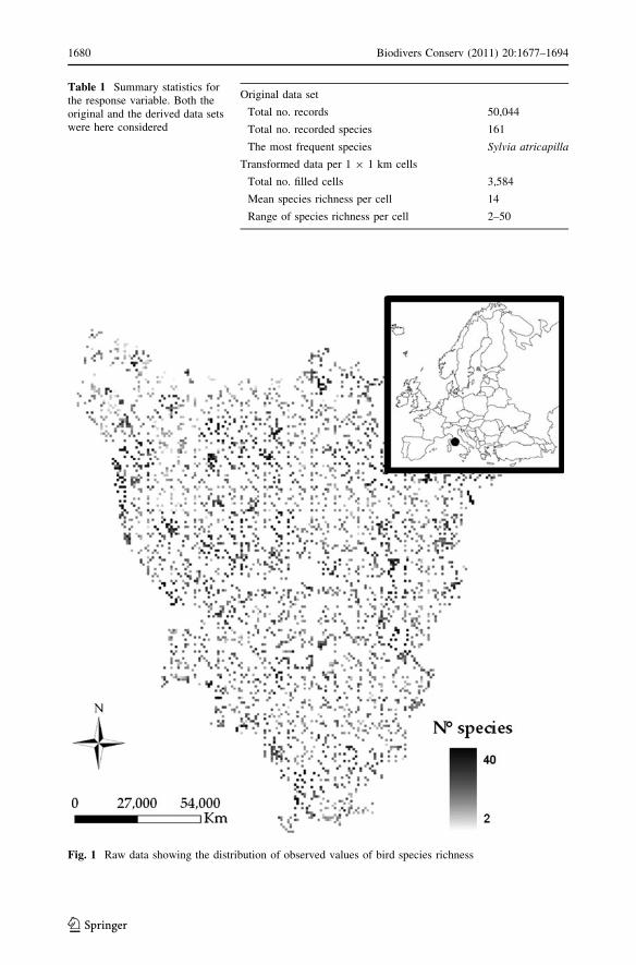
http://www.centrornitologicotoscano.org

Table 1 Summary statistics forthe response variable. Both theoriginal and the derived data setswere here considered

Original data set

Total no. records 50,044

Total no. recorded species 161

The most frequent species Sylvia atricapilla

Transformed data per 1 9 1 km cells

Total no. filled cells 3,584

Mean species richness per cell 14

Range of species richness per cell 2–50

Fig. 1 Raw data showing the distribution of observed values of bird species richness


123

Putative determinants of bird species richness

For each 1 9 1 km cell, three sets of predictor/explanatory variables were derived

(Table 2) and grouped according to a similarity criterion.

(I) Geographical features (four predictors): the coordinates for each grid cell (latitude

and longitude), elevation and distance to the sea were included in this group. Data on

topography and elevation was obtained from a digital elevation model (DEM) with a

resolution of 75 m by extracting the mean elevation for each grid cell. The minimum

distance to the sea was calculated for each grid cell, since this is one of the main geo-

graphical and ecological patterns in Tuscany, a region characterized by a marked asym-

metry with respect to the seaside.

(II) Landscape feature and complexity (four variables): Data on land cover were derived

from the third level of the CORINE Land Cover Map (see Bossard et al. 2000). For each

grid cell, the number of patches and the area (mean and standard deviation) covered by

each land cover class was calculated. Landscape shape complexity was calculated by using

the area weighted mean shape index (AWMSI). Starting from the shape index of each

patch, the mean shape index weighted on the relative area occupied by each patch is

obtained as:

AWMSI ¼XN

i¼1

Pi

2ffiffiffiffiffiffiffipAi

p� �

AiPNi¼1 Ai

!ð1Þ

where Pi and Ai are the perimeter and the area of each patch i within each 1 9 1 km grid

cell. Hence, the term Pi

2ffiffiffiffiffipAi

p� �

is the shape index of each patch i, which approximates 1

when the patch i has the simplest possible shape, i.e. the circle, and increases with

increasing patch shape complexity. We refer to McGarigal and Marks (1994) for a com-

plete description of this index while the relation of this index with fractal geometry has

been recently disentangled by Imre and Rocchini (2009).

The third level data of the CORINE Land Cover were used for calculating the Shannon

index according to the celebrated formula:

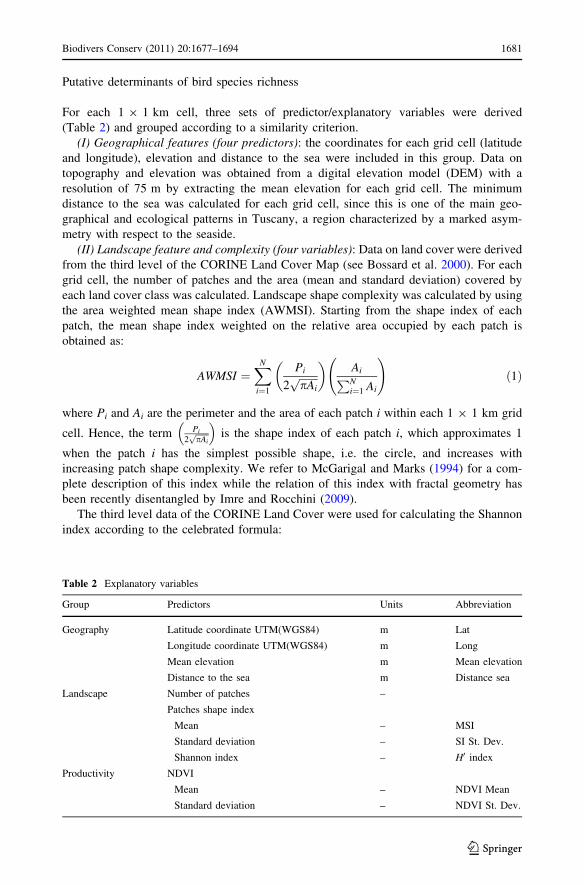
Table 2 Explanatory variables

Group Predictors Units Abbreviation

Geography Latitude coordinate UTM(WGS84) m Lat

Longitude coordinate UTM(WGS84) m Long

Mean elevation m Mean elevation

Distance to the sea m Distance sea

Landscape Number of patches –

Patches shape index

Mean – MSI

Standard deviation – SI St. Dev.

Shannon index – H0 index

Productivity NDVI

Mean – NDVI Mean

Standard deviation – NDVI St. Dev.


123

H0 ¼ �XM

C¼1

PC ln PCð Þ ð2Þ

where: H0 = Shannon diversity index, PC = proportion of the area occupied by each

class C.

(III) Primary productivity (two variables): normalized difference vegetation index

(NDVI) was used to discriminate between the amount of biomass characterising different

vegetation types. In order to extract the information required on the basis of continuous

spectral data, two ortho-Landsat ETM? images (path 192, row 029–030, acquisition date

20 June 2000; Bands 1–5 and 7 spatial resolution 28.5 m) were acquired from the Global

Land Cover Facility site hosted by the University of Maryland (htpp://glcfapp.umi-

acs.umd.edu). Complete information about image pre-processing is provided by Tucker

et al. (2004). June was chosen since it represents the period with maximum vegetation

spread in Mediterranean areas. NDVI was calculated as:

NDVI ¼ kNIR � kR

kNIR þ kRð3Þ

where kNIR is the reflectance in the NIR part of the spectrum (in such a case in the

0.76–0.90 lm electromagnetic window) and kR = reflectance in the Red part of the

spectrum (in such a case in the 0.63–0.69 lm electromagnetic window). NDVI varies from

a theoretical minimum of -1 (minimum reflectance in the NIR and maximum in the Red,

low biomass, e.g. sand) and a theoretical maximum of 1 (maximum reflectance in the NIR

and minimum in the Red, high biomass, e.g. woodland). NDVI is based on (i) the high

reflectance by vegetation in the NIR which is linked to scattering processes at the leaf scale

and (ii) the low reflectance in the Red due to the absorption by chloroplasts for photo-

synthesis (see Lillesand et al. 2004). Both NDVI standard deviation, as a proxy of envi-

ronmental heterogeneity, and mean NDVI, as a proxy of Net Primary Productivity, were

used.

Geostatistical modelling

Spatial autocorrelation of species richness and predictor variables is a general observed

feature of macro-ecological data sets (Hoeting et al. 2006). Its occurrence in the data can

have a more serious effect on model parameter estimation and it inflates type I errors of

traditional statistical tests (Kreft and Jetz 2007; Hoeting 2009). Some studies tried to

exclude spatial autocorrelation from regressive models (Ohlemuller et al. 2006), others, on

the contrary, explicitly addressed its role in shaping observed patterns of diversity (Bacaro

and Ricotta 2007; Kuhn 2007) and included it as a meaningful parameter in predictive

models (Pearson and Carroll 1999; Maes et al. 2005; Diggle and Ribeiro 2007).

A combined multi-predictor model was developed in this study, and it was further used

in conjunction with geostatistical techniques to predict birds diversity in 1 9 1 km grid

cells across the whole Tuscany region. In particular, the original data set, composed by

geo-referenced points (observations) was assembled to produce a regional map of bird

species richness.

Statistical modelling process was organised into the following three parts:

(1) Data transformation (normalization): generalized linear spatial models deal with a

variety of different data distributions (Poisson, Binomial, Gaussian—Diggle and


123

Ribeiro 2007). Counts data (e.g. the number of species in a grid cell) are usually

modelled assuming a Poisson distribution (and a log link function in order to avoid

predicted values lower than 0). However, over-dispersion (occurring when the ratio

between the mean and the variance of the response variable overpasses the value of 1)

implies to normalize the entire dataset and to deal with transformed Gaussian models

(Guisan and Zimmermann 2000; Guisan et al. 2002; Csontos et al. 2007). Hence,

since the number of observed bird species per 1 9 1 km grid cell showed over-

dispersion, a Box–Cox normalization (Box and Cox 1964; Legendre and Legendre

1998) was adopted and the lambda (k) parameter was estimated by maximising the

log-likelihood profile.

(2) Building the generalized linear spatial model: once the response variable (number of

bird species) at each grid cell within the Tuscany region was denoted as:

ðxi; yiÞ : i ¼ 1; :. . .; n ð4Þ

where xi identifies the spatial location (in two-dimensional space—longitude and

latitude expressed in kilometres) and yi is the bird richness value associated with the

location xi, a geostatistical (isotropic) model can be defined as:

Yi ¼ SðxiÞ þ Zi : i ¼ 1; . . .::; n ð5Þ

where

SðxÞ : x 2 <2� �

ð6Þ

is a Gaussian process with a spatially varying mean l(x) defined by a classical linear

regression model such as:

lðxÞ ¼ b0 þ bjpj ð7Þ

with pj (j = 1,….,s) expressing the jth explanatory variable p.

The described Gaussian process is also characterized by a variance given by:

r2 ¼ Var SðxÞf g ð8Þ

and by a positive-defined correlation function:

qðuÞ ¼ Corr SðxÞ; Sðx0Þf g ð9Þ

defining the way correlation function decays to zero for increasing distances occur-

ring between observations at locations x and x0. In Eq. 5, the model formulation

includes the term Zi representing mutually independent N(0, s2) random variables (or

simply the error term; refers to Diggle and Ribeiro 2007 for mathematical and sta-

tistical details).

Considering all the above described terms, the fitting of a generalized linear spatial

model was accomplished by a step-by-step procedure. Firstly, explanatory variables

for modelling the large-scale variation in bird diversity were chosen via a model

selection technique (the Akaike Information Criterion, AIC). In order to detect

multicollinearity in the set of predictors, a general explorative analysis of pairwise

variable correlations (using Pearson’s correlation coefficients, Appendix I) was car-

ried out. Multicollinearity represents a factor with a strong influence on model

development and especially on the selection of subsets of predictors during stepwise

model building (for a discussion on the matter, see Fox 2008), leading to the


123

exclusion of important factors from models (i.e. when strong collinearity was

observed, the inclusion/exclusion of a variable in the final model is mainly due to the

order that variable is added to the model).

A reduced linear model (including only those explanatory variables resulted mean-

ingful) was then calculated in order to describe the spatially varying mean related of

the number of bird species. Via AIC, the best predictor subset was finally obtained

and regression coefficients estimated (see Eq. 7).

Secondly, the residuals from the model were examined for spatial correlation

and a suitable family of correlations was chosen (Hoeting et al. 2006).

Explicitly, the spatial relationships in bird data residuals were modelled com-

puting an empirical variogram for a vector h of distance classes. The following

classical parameters for the autocorrelative spatial structure (theoretical vario-

gram) were then estimated (see Pearson and Carroll 1999; Diggle and Ribeiro

2007): nugget (s2, representing the intercept of the variogram), sill (s2 þ r2,

expressed as the difference between the asymptote and the nugget of the vario-

gram) and range (u, indicating the distance at which the theoretical variogram

reaches its maximum). For convenience, a practical range is also defined as the

distance at which the correlation function reaches the value of 0.05. However,

since the estimation of the above described spatial parameters strongly depends on

the selection of the correlation function q(u), different fits of a parametric Matern

(1986) function of order k with respect to the empirical variogram were obtained

and the correct correlation function (able to maximize the likelihood estimation)

was selected.

From a practical point of view, the estimates of the parameters in the trend surface

(model spatial component) were updated using an optimisation function (as

described in Nelder and Mead 1965) followed by maximum likelihood estimation

of the parameters of the covariance function using the residuals (Ribeiro and

Diggle 2001). In this dynamic process, the inclusion of one or more important

explanatory variables could drastically change or reduce the correlation structure

of the residuals from the model (Hoeting et al. 2006). Cross-validation statistics by

leave-one-out procedure were used to assess the bias and the accuracy of the final

spatial model.

(3) Universal kriging (Krige 1976) was finally applied in order to predict expected bird

richness (and its variation) in each 1 9 1 km grid cell across the whole Tuscany

Region for those grid cells where the retained predictors were available. All analyses

were performed using the R software (R Development Core Team 2011) and the

geoR package (Ribeiro and Diggle 2001).

Results

Overall, the analysed data-set was composed by a huge number of observations (see

Table 1). The most frequent species was the blackcap, Sylvia atricapilla, which was

recorded in 2,696 1 9 1 km cells. Once the geographical 1 9 1 km grid for the whole

Tuscany was overlaid with respect to the set of spatially-explicited bird occurrences, the

total number of non-empty cells was 3,584 and the mean calculated species richness per

cell was 14 (with a minimum of 2 and a maximum of 50, see Table 1 and Fig. 1). The total

number of species (161) represents 60.8% of the whole richness of the diurnal Italian


123

breeding birds (265 species, CISO 2010). Moreover, considering the sum of regular,

irregular and accidental breeders (AERC categories A and C breeding status 1, 2 and 3),

Tuscany accounts for 188 species (Arcamone and Baccetti 2004), 85.63 of which detected

during our monitoring program.

The rarefaction curve based on the species composition of these filled cells (Fig. 2)

showed a clear asymptotic pattern after 1/3 (about 1,000) cells were cumulated. The

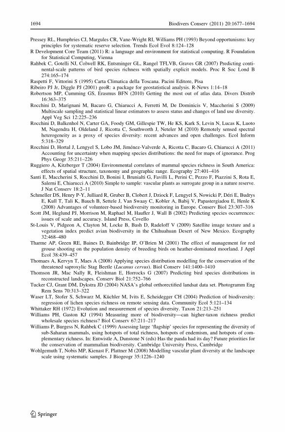
distribution of the number of species per cells (Fig. 3) was far from a Gaussian distribution

(this was confirmed by the Shapiro–Wilk normality test: W = 0.930, P \ 0.001) showing a

skewed shape (Fig. 3). For this reason, the number of bird species per cell grid was

normalized using a Box–Cox power of 0.184 (Table 3). After stepwise selection, only four

predictors (out of the ten variables tested, Table 2) were included in the model (Table 3).

Multicollinearity in retained predictors was absent (Appendix 1).

Fig. 2 Rarefaction curve based on the random accumulation of 3,584 1 9 1 km cells

N° species

Fre

quen

cy

0 10 20 30 40 50

050

100

150

200

250

300Fig. 3 Histogram of species no.

frequencies. A skeweddistribution can be observed (lackof normality)


123

The NDVI standard deviation showed a positive correlation with birds species richness

and it was the most predictive variable included in the reduced model, in terms of

explanatory power. The second predictor was represented by the landscape heterogeneity

quantified by the H0 index calculated on the land cover data. Mean elevation of the cell

entered into the model with a minor negative coefficient, while distance from the sea

entered in the model with a weak positive relationship. The intercept of the estimated

spatial varying mean resulted highly significant and was, consequently, included in the

model. Its value expresses the mean of the (transformed) number of bird species in each

grid cell irrespective of the environmental and spatial parameters.

Table 3 Description of explan-atory variables (and their associ-ated coefficients) included afterstepwise selection in the spatialvarying mean component(***P \ 0.001)

Estimated value

Trend parameters (spatial varying mean)

Intercept 3.066***

NDVI St. Dev. 0.811***

H0 index 0.104***

Mean elevation -0.001***

Distance sea [0.001***

Spatial parameters

Nugget (s2) 0.147

Partial sill (r2) 0.270

Range (u) 0.054

Practical range 0.162

Normalisation parameter (Box–Cox power)

Lambda (k) 0.184

Covariance function parameters (Matern)

Order (k) 0.5 (exponential model)

0.00 0.05 0.10 0.15 0.20 0.25 0.30

0.10

0.15

0.20

0.25

0.30

0.35

0.40

0.45

Distance classes (km-2)

Sem

ivar

ianc

e

Fig. 4 Plot of the empirical(circles) and fitted (solid line)semivariograms vs. distance(km-2) obtained using theresiduals after the spatial varyingmean was subtracted by raw(normalized) data


123

On the other side, the modeled spatial parameters highlighted that autocorrelation in

bird richness value existed and strongly influenced the number of observed species. In

particular, the practical range was reached after 16 km, indicating the absence of further

correlative structure in data after this threshold (see Fig. 4 and Table 3). Moreover, the

nugget parameter, expressing the unexplained variance (occurring at a spatial scale lower

than that here analyzed) was 0.147. Relatively to the covariance function used to model the

empirical variogram, the k = 0.5 parameter was selected (corresponding to fit an expo-

nential theoretical variogram with respect to the observed data).

Predicted Birds Richness

Obs

erve

d B

irds

Ric

hnes

s

0 10 20 30 40 50

010

2030

4050

6.0 6.5 7.0 7.5

47.0

47.5

48.0

48.5

49.0

Coord X

Coo

rd Y

a

b

Fig. 5 Cross-validation for thefinal adopted model; a observedvs. predicted (following Pineiroet al. 2008) birds richness (thecontinuous line represents theexpected regression line for amodel with perfect prediction);b error map for observed vs.predicted birds richness (‘‘?’’symbols are used to indicate apositive error while ‘‘9’’ fornegative; in the same way,symbol’s dimension express theabsolute value of the calculatederror)


123

Predicted values were significantly related with observed bird richness (R2 = 0.448,

P \ 0.001, Fig. 5a). For comparison, a simple multiple regression model without the

inclusion of the spatial component in the analysis, showed a lower R2 value (R2 = 0.15,

P \ 0.001).

It is interesting to note an underestimate of predicted bird species richness for those

grids with high species richness. The transformation adopted (quasi-logarithmic) is the

major determinant for this observed pattern: in fact, it should be considered that the use of

a logarithmic transformation tend to reduce the total variability with respect to the original

dataset and, for this reason, predictions (when back-transformed in the original measure-

ment scale, e.g. no. of species) show this typical pattern.

The model errors (observed data - predicted value) were equally-distributed

throughout the whole region (Fig. 5b) confirming that the data were sampled with a

comparable accuracy throughout the whole region. Predicted bird richness (and its asso-

ciated variance) across all the Tuscan region is shown in Fig. 6.

Discussion

In this article we demonstrated the powerfulness of ancillary geographic and ecological

data (in particular, landscape heterogeneity rather than elevation) at different spatial scales

for predicting bird biodiversity, as a powerful throughput for species richness geostatistical

modeling. Moreover, we showed as it is possible to model the spatially explicit nature of

data recorded on a geographical map (e.g. Atlases). Atlases play an important role in

biodiversity conservation by providing essential data on the occurrence of species

(Robertson et al. 2010). Even if data based on atlases are not derived by a systematic

sampling procedure, the temporal and spatial spread of censuses provide relative reliable

Fig. 6 Regional pattern of bird species richness as expected under the described geostatistical model.a Expected birds species richness and b its expected variance


123

data, yielding unbiased results (Hortal and Lobo 2006). Schmeller et al. (2008) found a

positive relationship between the sampling intensity (intended as number of observers or of

visits per site) and the number of recorded species. These authors straightforwardly con-

cluded that a direct influence exists between the number of people involved in a census and

the accuracy of bird richness data. Of course, large sampling effort could counterbalance

hypothesized measurement errors in data collected by operators (avoiding the underesti-

mate of rare species, Hochachka et al. 2000; Schmeller et al. 2008). Considering the

sampling effort for the Tuscan bird census, the almost asymptotic pattern of the rarefaction

curve suggests that the analyzed dataset was adequate to study the overall bird diversity

across the Tuscan region.

Model and predictors assessment

Increasingly, ecologists are involved in the prediction of spatial or temporal patterns of

ecological or biodiversity variables (Begon et al. 2006). The estimation of the geographical

distribution of species richness is one of the most investigated topics in ecology and

conservation biology, because of two main reasons: (i) to understand the ecological and

evolutionary patterns of biodiversity (Kreft and Jetz 2007; Pineda and Lobo 2009) and (ii)

to focus on those areas of emerging biodiversity value (hotspots) that require conservation

actions.

By applying geostatistical models, a well-performing predictive model was obtained for

the distribution of bird species richness in Tuscany by considering relatively few variables,

namely a combination of the variability in habitat productivity (NDVI), habitat heterogeneity

(H0 index), combined with topographic (elevation) and geographic (distance from the sea)

information. Overall, the calculated R2 is similar to those obtained for other predictive models

developed in a number of different geographical areas (see for example Jetz and Rahbek

2002; Rahbek et al. 2007). The highlighted relationships occurring between bird richness and

heterogeneity-based predictors (i.e. NDVI standard deviation and Shannon H0) pointed out

that the higher the environmental heterogeneity of an area the higher will be the diversity of

species living therein (see Gillespie et al. 2008 or Rocchini et al. 2010 for a review on previous

studies demonstrating similar patterns). In this view, remotely sensed information has been

proven to be a powerful tool for detecting environmental variability by relying on the vari-

ability in the spectral response of habitats, as detected by a remote sensor (Nagendra and

Rocchini 2008; He et al. 2009). Hence, ancillary variables based on remotely sensed infor-

mation (e.g. NDVI or Shannon H0 derived from a classified image) can be used as powerful

tools to model the spatial variation of bird species richness and locate biodiversity hotspots.

The theoretical assumption beyond the use of remotely sensed variability considering both

continuous (e.g. NDVI) or classified (e.g. Shannon H0 of landscape structure) data to predict

species richness is based on the Spectral Variation Hypothesis (see Palmer et al. 2002)—i.e.

higher spectral variability should correspond to higher species diversity—and it has been

proven true for different taxa including vascular plants (Gould 2000; Foody and Cutler 2003;

Fairbanks and McGwire 2004; Kumar et al. 2006), lichens (Waser et al. 2004), birds (Goetz

et al. 2007; St-Louis et al. 2009) and mammals (Oindo and Skidmore 2002). This is in line

with the Niche Difference Hypothesis (see Nekola and White 1999)—i.e. diverse habitats

show a higher diversity in species composition on the strength of a higher number of available

niches; according to this hypothesis bird species richness is expected to be higher where a

higher vegetation heterogeneity exists, since different vegetation types would result in a

larger number of niches for birds (Whittaker 1972). The relation between bird species rich-

ness and vegetation complexity has been demonstrated at different spatial scales and in


123

different ecosystems (MacArthur et al. 1966, Rahbek et al. 2007). In Tuscany, a positive

relation between bird species richness and plant species richness has been demonstrated at the

local scale within the Sant’Agnese Nature reserve (Santi et al. 2010). From a very general

point of view, differences in habitat type and quality are well known to shape the occurrence

of avian species in different landscapes (see Tharme et al. 2001; Rahbek et al. 2007).

Noteworthy, the model obtained in this study showed a large amount of unexplained variance;

one possibility for future model improvement will be represented by the inclusion of other

important predictors currently not considered, such as climate (Rahbek et al. 2007; Doswald

et al. 2009), net primary productivity (Jetz and Rahbek 2002), other measures of habitat

heterogeneity (Guegan et al. 1998) or distribution of highly related organisms (Pearson and

Carroll 1999). Moreover, partitioning regional species pool into specific guilds (for instance

rare vs. widespread species) would represent a possible direction in order to ameliorate such a

class of predictive models. Many studies (Jetz and Rahbek 2002; Lennon et al. 2004; Rug-

giero and Kitzberger 2004; Rahbek et al. 2007; Bacaro et al. 2008) suggested that statistical

associations between total species richness and environmental predictors could be misleading

owing to the dominating influence of common species whereas both theoretical (Bacaro and

Ricotta 2007) and empirical (Lennon et al. 2004; Rahbek et al. 2007) evidences described

species with small geographical ranges and relative low abundance as responsible for peaks of

observed species richness.

In term of its usefulness, the spatial model developed in this work could be seen as a tool for

different aims: firstly, as above mentioned, on the basis of these models it is possible to plan

conservation strategies looking at the presence of biodiversity hotspots not ‘‘covered’’ by

conservation tools (e.g. natural reserves, for an example see Thomaes et al. 2008).

Obviously, when concrete conservation actions are scheduled based on model predic-

tions alone, field controls or the inclusion of other data (such as other available records of

species occurrence) are necessary. Secondly, spatial predictions may suggest how and

where sampling activities should be performed: advices for both retrospective and pro-

spective sampling design (sensu Diggle and Ribeiro 2007) will be easily extrapolated

considering the variance related to the predicted mean, driving sampling effort throughout

a more efficient direction. Such an approach is likely to lead to substantial conservation

gain if future reserve networks could be designed and implemented to account for the

‘‘black holes’’ in our knowledge, mainly generated by a non adequate sampling effort.

From a methodological point of view, geostatistical models own the advantage to

incorporate information of environmental co-variation and neighborhood effects (Kreft and

Jetz 2007), improving the quality of predictions. Nonetheless, there is a number of dis-

advantages of ignoring spatial correlation in model selection procedures leading, for

example, to (i) the exclusion of relevant covariates in the final model (Hoeting et al. 2006)

or (ii) higher prediction errors for estimation of the response (Hoeting 2009).

Acknowledgments The Monitoring Program of Breeding Birds was funded by the ‘‘Regione Toscana’’.We would like to acknowledge Noam Levin who provided constructive comments to a previous version ofthis manuscript. Part of this work was done by the first author (GB) during a visiting research period at theInstitute of Hazard, Risk and Resilience, Department of Geography, University of Durham (UK), founded bythe ‘‘Luigi and Francesca Brusarosco’’ Foundation. DR is partially funded by the Autonomous Province ofTrento (Italy), ACE-SAP project (No. 23, June 12, 2008, of the University and Scientific Research Service).

Appendix

See Table 4.


123

References

Araujo MB, Guisan A (2006) Five (or so) challenges for species distribution modelling. J Biogeogr33:1677–1688

Arcamone E, Baccetti B (2004) Check-list COT degli uccelli toscani. www.centrornitologicotoscano.orgAustin MP (2002) Spatial prediction of species distribution: an interface between ecological theory and

statistical modelling. Ecol Model 157:101–118Austin MP, Belbin L, Meyers JA, Doherty MD, Luoto M (2006) Evaluation of statistical models used for

predicting plant species distributions: role of artificial data and theory. Ecol Model 199:197–216Bacaro G, Ricotta C (2007) A spatially explicit measure of beta diversity. Community Ecol 8:41–46Bacaro G, Ricotta C (2009) L’uso di dati da Atlante per misurare la beta-diversita. In: Amori G, Battisti C,

De Felici S (eds) I Mammiferi della Provincia di Roma. Dallo stato delle conoscenze alla gestione econservazione delle specie. Provincia di Roma, Assessorato alle politiche dell’Agricoltura, Stilgrafica,Roma

Bacaro G, Rocchini D, Bonini I, Marignani M, Maccherini S, Chiarucci A (2008) The role of regional andlocal scale predictors for plant species richness in Mediterranean forests. Plant Biosyst 142:630–642

Bacaro G, Baragatti E, Chiarucci A (2009) Using taxonomic data for assessing and monitoring biodiversity:are the tribes still fighting? J Environ Monit 11:798–801

Baffetta F, Bacaro G, Fattorini L, Rocchini D, Chiarucci A (2007) Multi-stage cluster sampling for esti-mating average species richness at different spatial grains. Community Ecol 8:119–127

Bani L, Massimino D, Bottoni L, Massa R (2006) A multiscale method for selecting indicator species andpriority conservation areas: a case study for broadleaved forests in Lombardy, Italy. Conserv Biol20:512–526

Barbaro L, Rossi JP, Vetillard F, Nezan J, Jactel H (2006) The spatial distribution of birds and carabidbeetles in pine plantation forests: the role of landscape composition and structure. J Biogeogr34:652–664

Begon M, Townsend CA, Harper JL (2006) Ecology: from individuals to ecosystems, 4th edn. Blackwell,Oxford

Bibby CJ, Burgess ND, Hill DA, Mustoe SH (2000) Bird census techniques, 2nd edn. Academic, LondonBino G, Levin N, Darawshi S, Van Der Hal N, Reich-Solomon A, Kark S (2008) Accurate prediction of bird

species richness patterns in an urban environment using Landsat-derived NDVI and spectral unmixing.Int J Remote Sens 29:3675–3700

Table 4 Matrix of correlation coefficients (Pearson’s product moment) for the set of variables used as birdspecies richness predictors

Meanelevation

Distanceto thesea

Numberofpatches

Patchesshapeindex—mean

Patchesshape index—St. Dev.

Shannonindex

NDVImean

NDVISt.Dev.

Mean elevation 1.00 0.30 -0.12 0.10 0.04 -0.13 0.66 -0.40

Distance tothe sea

0.30 1.00 0.10 -0.08 -0.01 0.07 0.16 0.02

Number ofpatches

-0.12 0.10 1.00 -0.80 -0.23 0.79 -0.09 0.33

Patches shapeindex—mean

0.10 -0.08 -0.80 1.00 -0.18 -0.76 0.09 -0.32

Patches shapeindex—St. Dev.

0.04 -0.01 -0.23 -0.18 1.00 -0.32 0.05 -0.13

Shannon index -0.13 0.07 0.79 -0.76 -0.32 1.00 -0.14 0.38

NDVI mean 0.66 0.16 -0.09 0.09 0.05 -0.14 1.00 -0.51

NDVI St. Dev. -0.40 0.02 0.33 -0.32 -0.13 0.38 -0.51 1.00


123

http://www.centrornitologicotoscano.org

Block WM, Brennan LA (1993) The habitat concept in ornithology. Curr Ornithol 11:35–91Bossard M, Feranec J, Otahel J (2000) CORINE land cover technical guide—addendum 2000. Technical

report no. 40. European Environment Agency, CopenhagenBox GEP, Cox DR (1964) An analysis of transformations. J Roy Stat Soc B 26:211–246Cabeza M, Araujo MB, Wilson RJ, Thomas CD, Cowley MJR, Moilanen A (2004) Combining probabilities

of occurrence with spatial reserve design. J Appl Ecol 41:252–262Carroll SS, Pearson DL (1998) Spatial modeling of butterfly species richness using tiger beetles (Cicin-

delidae) as a bioindicator taxon. Ecol Appl 8:531–543Centro Italiano Studi Ornitologici (CISO) (2010) http://www.ciso-coi.org/Chiarucci A, Bacaro G, Rocchini D, Fattorini L (2008) Discovering and rediscovering the sample-based

rarefaction formula in ecological literature. Community Ecol 9:121–123Cody ML (1985) Habitat Selection in Birds. Academic, OrlandoCooper SD, Barmuta L, Sarnelle O, Kratz K, Diehl S (1997) Quantifying spatial heterogeneity in streams.

J N Am Benthol Soc 16:174–188Cressie N (1990) The origins of kriging. Math Geol 22:239–252Csontos P, Rocchini D, Bacaro G (2007) Modelling factors affecting litter mass components of pine stands.

Community Ecol 8:247–256Currie DJ, Mittelbach GG, Cornell HV, Field R, Guegan JF, Hawkins BA, Kaufman DM, Kerr JT, Obe-

rdorff T, O’Brien E, Turner JRG (2004) Predictions and tests of climate-based hypotheses of broad-scale variation in taxonomic richness. Ecol Lett 7:1121–1134

Dalthorp D (2004) The generalized linear model for spatial data: assessing the effects of environmentalcovariates on population density in the field. Entomol Exp Appl 111:117–131

Diggle PJ, Ribeiro PJ Jr (2007) Model-based Geostatistics. Springer, New YorkDoswald N, Willis SG, Collingham YC, Pain DJ, Green RE, Huntley B (2009) Potential impacts of climatic

change on the breeding and non-breeding ranges and migration distance of European Sylvia warblers.J Biogeogr 36:1194–1208

Fairbanks DHK, McGwire KC (2004) Patterns of floristic richness in vegetation communities of California:regional scale analysis with multi-temporal NDVI. Glob Ecol Biogeogr 13:221–235

Field R, O’Brien EM, Whittaker RJ (2005) Global models for predicting woody plant richness from climate:development and evaluation. Ecology 86:2263–2277

Foody GM, Cutler MEJ (2003) Tree biodiversity in protected and logged Bornean tropical rain forests andits measurement by satellite remote sensing. J Biogeogr 30:1053–1066

Fox J (2008) Applied regression analysis and generalized linear models, 2nd edn. Sage, Thousand OaksGillespie TW, Foody GM, Rocchini D, Giorgi AP, Saatchi S (2008) Measuring and modelling biodiversity

from space. Prog Phys Geogr 32:203–221Goetz S, Steinberg D, Dubayah R, Blair B (2007) Laser remote sensing of canopy habitat heterogeneity as a

predictor of bird species richness in an eastern temperate forest, USA. Remote Sens Environ108:254–263

Goovaerts P (1997) Geostatistics for natural resources evaluation. Oxford University Press, New YorkGotelli NJ, Colwell RK (2001) Quantifying biodiversity: procedures and pitfalls in the measurement and

comparison of species richness. Ecol Lett 4:379–391Gould W (2000) Remote Sensing of vegetation, plant species richness, and regional biodiversity hot spots.

Ecol Appl 10:1861–1870Gregory RD, Noble DG, Custance J (2004) The state of play of farmland birds: population trends and

conservation status of lowland farmland birds in the United Kingdom. Ibis 146:1–13Guegan JF, Lek S, Oberdorff T (1998) Energy availability and habitat heterogeneity predict global riverine

fish diversity. Nature 391:382–384Guisan A, Zimmermann NE (2000) Predictive habitat distribution models in ecology. Ecol Model

135:147–186Guisan A, Edwards J, Hastie T (2002) Generalized linear and generalized additive models in studies of

species distributions: setting the scene. Ecol Model 157:89–100He KS, Zhang J, Zhang Q (2009) Linking variability in species composition and MODIS NDVI based on

beta diversity measurements. Acta Oecol 35:14–21Hochachka WM, Martin K, Doyle F, Krebs CJ (2000) Monitoring vertebrate populations using observa-

tional data. Can J Zool 78:521–529Hoeting JA (2009) The importance of accounting for spatial and temporal correlation in analyses of

ecological data. Ecol Appl 19:574–577Hoeting JA, Davis RA, Merton AA, Thompson SE (2006) Model selection for geostatistical models. Ecol

Appl 16:87–98


123

http://www.ciso-coi.org/

Hortal J, Lobo JM (2006) Towards a synecological framework for systematic conservation planning.Biodivers Inform 3:16–45

Imre A, Rocchini D (2009) Explicitly accounting for pixel dimension in calculating classical and fractallandscape shape metrics. Acta Biotheor 57:249–360

Jetz W, Rahbek C (2002) Geographic range size and determinants of avian species richness. Science297:1548–1551

Kark S, Allnutt TF, Levin N, Manne LL, Williams PH (2007) The role of transitional areas as avianbiodiversity centres. Global Ecol Biogeogr 16:187–196

Kati V, Devillers P, Dufrene M, Legakis A, Vokou D, Lebrun P (2004) Testing the value of six taxonomicgroups as biodiversity indicators at a local scale. Conserv Biol 18:667–675

Kobayashi S (1974) The species-area relation I. A model for discrete sampling. Res Popul Ecol 15:223–237Koellner T, Hersperger A, Wohlgemuth T (2004) Rarefaction method for assessing plant species diversity

on a regional scale. Ecography 27:544, 532Kreft H, Jetz W (2007) Global patterns and determinants of vascular plant diversity. Proc Natl Acad Sci

104:5925–5930Krige DG (1966) Two-dimensional weighted moving average trend surfaces for ore-evaluation. J S Afr Inst

Min Metall 66:13–38Krige DG (1976) A review of the development of geostatistics in South Africa. In: Guarascio M, David M,

Huijbregts C (eds) Advanced geostatistics in the mining industry. Reidel, Dordrecht, pp 279–293Kuhn I (2007) Incorporating spatial autocorrelation may invert observed patterns. Divers Distrib 13:66–69Kumar S, Stohlgren TJ, Chong GW (2006) Spatial heterogeneity influences native and nonnative plant

species richness. Ecology 87:3186–3199Legendre P (1993) Spatial autocorrelation: trouble or new paradigm? Ecology 74:1659–1673Legendre P, Legendre L (1998) Numerical ecology, second english edn. Elsevier, AmsterdamLennon JJ, Koleff P, Greenwood JJD, Gaston KJ (2004) Contribution of rarity and commonness to patterns

of species richness. Ecol Lett 7:81–87Lillesand TM, Kiefer RW, Chipman JW (2004) Remote sensing and image interpretation, 5th edn. Wiley,

New YorkMacArthur RH, Recher H, Cody M (1966) On the relation between habitat selection and species diversity.

Am Nat 100:319–332Maccherini S, Bacaro G, Favilli L, Piazzini S, Santi E, Marignani M (2009) Congruence among butterflies

and vascular plants in evaluation of grassland restoration success. Acta Oecol 35:311–317Maes D, Bauwens D, De Bruyn L, Anselin A, Vermeersch G, Van Landuyt W, De Knijf G, Gilbert M (2005)

Species richness coincidence: conservation strategies based on predictive modelling. Biodivers Con-serv 14:1345–1364

Matern B (1986) Spatial variation, 2nd edn. Springer, BerlinMatheron G (1963) Principles of geostatistics. Econ Geol 58:1246–1266McGarigal K, Marks BJ (1994) FRAGSTATS: spatial pattern analysis program for quantifying landscape

structure. Department of Agriculture, Forest Service, Pacific Northwest Research Station, PortlandNagendra H, Rocchini D (2008) High resolution satellite imagery for tropical biodiversity studies: the devil

is in the detail. Biodivers Conserv 17:3431–3442Nekola JC, White PS (1999) The distance decay of similarity in biogeography and ecology. J Biogeogr

26:867–878Nelder JA, Mead R (1965) A simplex algorithm for function minimization. Comput J 7:308–313Ohlemuller R, Walker S, Bastow Wilson J (2006) Local vs regional factors as determinants of the inva-

sibility of indigenous forest fragments by alien plant species. Oikos 112:493–501Oindo BO, Skidmore AK (2002) Interannual variability of NDVI and species richness in Kenya. Int J

Remote Sens 23:285–298Palmer MW, Earls P, Hoagland BW, White PS, Wohlgemuth T (2002) Quantitative tools for perfecting

species lists. Environmetrics 13:121–137Pearson DL, Carroll SS (1999) The influence of spatial scale on cross-taxon congruence patterns and

prediction accuracy of species richness. J Biogeogr 26:1079–1090Pineda E, Lobo JM (2009) Assessing the accuracy of species distribution models to predict amphibian

species richness patterns. J Anim Ecol 78:182–190Pineiro G, Perelman S, Guerschman JP, Paruelo JM (2008) How to evaluate models: observed vs. predicted

or predicted vs. observed? Ecol Modell 216:316–322Polasky S, Solow AR (2001) The value of information in reserve site selection. Biodivers Conserv

10:1051–1058Prendergast JR, Quinn RM, Lawton JH, Eversham BC, Gibbons DW (1993) Rare species, the coincidence of

diversity hotspots and conservation strategies. Nature 365:335–337


123

Pressey RL, Humphries CJ, Margules CR, Vane-Wright RI, Williams PH (1993) Beyond opportunisms: keyprinciples for systematic reserve selection. Trends Ecol Evol 8:124–128

R Development Core Team (2011) R: a language and environment for statistical computing. R Foundationfor Statistical Computing, Vienna

Rahbek C, Gotelli NJ, Colwell RK, Entsminger GL, Rangel TFLVB, Graves GR (2007) Predicting conti-nental-scale patterns of bird species richness with spatially explicit models. Proc R Soc Lond B274:165–174

Raspetti F, Vittorini S (1995) Carta Climatica della Toscana. Pacini Editore, PisaRibeiro PJ Jr, Diggle PJ (2001) geoR: a package for geostatistical analysis. R-News 1:14–18Robertson MP, Cumming GS, Erasmus BFN (2010) Getting the most out of atlas data. Divers Distrib

16:363–375Rocchini D, Marignani M, Bacaro G, Chiarucci A, Ferretti M, De Dominicis V, Maccherini S (2009)

Multiscale sampling and statistical linear estimators to assess status and changes of land use diversity.Appl Veg Sci 12:225–236

Rocchini D, Balkenhol N, Carter GA, Foody GM, Gillespie TW, He KS, Kark S, Levin N, Lucas K, LuotoM, Nagendra H, Oldeland J, Ricotta C, Southworth J, Neteler M (2010) Remotely sensed spectralheterogeneity as a proxy of species diversity: recent advances and open challenges. Ecol Inform5:318–329

Rocchini D, Hortal J, Lengyel S, Lobo JM, Jimenez-Valverde A, Ricotta C, Bacaro G, Chiarucci A (2011)Accounting for uncertainty when mapping species distributions: the need for maps of ignorance. ProgPhys Geogr 35:211–226

Ruggiero A, Kitzberger T (2004) Environmental correlates of mammal species richness in South America:effects of spatial structure, taxonomy and geographic range. Ecography 27:401–416

Santi E, Maccherini S, Rocchini D, Bonini I, Brunialti G, Favilli L, Perini C, Pezzo F, Piazzini S, Rota E,Salerni E, Chiarucci A (2010) Simple to sample: vascular plants as surrogate group in a nature reserve.J Nat Conserv 18:2–11

Schmeller DS, Henry P-Y, Julliard R, Gruber B, Clobert J, Dziock F, Lengyel S, Nowicki P, Deri E, BudrysE, Kull T, Tali K, Bauch B, Settele J, Van Swaay C, Kobler A, Babij V, Papastergiadou E, Henle K(2008) Advantages of volunteer-based biodiversity monitoring in Europe. Conserv Biol 23:307–316

Scott JM, Heglund PJ, Morrison M, Raphael M, Haufler J, Wall B (2002) Predicting species occurrences:issues of scale and accuracy. Island Press, Covello

St-Louis V, Pidgeon A, Clayton M, Locke B, Bash D, Radeloff V (2009) Satellite image texture and avegetation index predict avian biodiversity in the Chihuahuan Desert of New Mexico. Ecography32:468–480

Tharme AP, Green RE, Baines D, Bainbridge IP, O’Brien M (2001) The effect of management for redgrouse shooting on the population density of breeding birds on heather-dominated moorland. J ApplEcol 38:439–457

Thomaes A, Kervyn T, Maes A (2008) Applying species distribution modelling for the conservation of thethreatened saproxylic Stag Beetle (Lucanus cervus). Biol Conserv 141:1400–1410

Thomson JR, Mac Nally R, Fleishman E, Horrocks G (2007) Predicting bird species distributions inreconstructed landscapes. Conserv Biol 21:752–766

Tucker CJ, Grant DM, Dykstra JD (2004) NASA’s global orthorectified landsat data set. Photogramm EngRem Sens 70:313–322

Waser LT, Stofer S, Schwarz M, Kuchler M, Ivits E, Scheidegger CH (2004) Prediction of biodiversity:regression of lichen species richness on remote sensing data. Community Ecol 5:121–134

Whittaker RH (1972) Evolution and measurement of species diversity. Taxon 21:213–251Williams PH, Gaston KJ (1994) Measuring more of biodiversity—can higher-taxon richness predict

wholesale species richness? Biol Conserv 67:211–217Williams P, Burgess N, Rahbek C (1999) Assessing large ‘flagship’ species for representing the diversity of

sub-Saharan mammals, using hotspots of total richness, hotspots of endemism, and hotspots of com-plementary richness. In: Entwistle A, Dunstone N (eds) Has the panda had its day? Future priorities forthe conservation of mammalian biodiversity. Cambridge University Press, Cambridge

Wohlgemuth T, Nobis MP, Kienast F, Plattner M (2008) Modelling vascular plant diversity at the landscapescale using systematic samples. J Biogeogr 35:1226–1240


123

Geostatistical modelling of regional bird species richness: exploring environmental proxies for conservation purpose

Documents