Geostatistical investigation of ETEX-1: Structural analysis

ARTICLE IN PRESS

1352-2310/$ - se

doi:10.1016/j.at

�CorrespondE-mail addr

Atmospheric Environment 39 (2005) 1683–1693

www.elsevier.com/locate/atmosenv

Geostatistical investigation of ETEX-1: Structural analysis

Gregoire Duboisa,�, Stefano Galmarinia, Michaela Saisanab

aRadioactivity Environmental Monitoring, Institute for Environment and Sustainability, Joint Research Centre,

European Commission, TP 441, Via E Fermi, 21020 Ispra (VA), ItalybApplied Statistics, Institute for the Protection and Security of the Citizen, Joint Research Centre, European Commission,

TP 361, Via E Fermi, 21020 Ispra (VA), Italy

Received 5 August 2004; received in revised form 5 November 2004; accepted 17 November 2004

Abstract

The surface concentration data collected during the European Tracer Experiment (ETEX) are analysed for the first

time by means of geostatistical techniques. The aim of the analysis is to determine the self-consistency of the data, to

identify anomalous behaviours of stations with respect to the spatial and time structure of the tracer cloud

measurements and to characterise the correlation structure of the measured cloud. The so-called structural analysis is

usually regarded as the investigation step to be conducted prior to any interpolation procedure and mapping. Given the

relevance of the ETEX dataset, one of the few existing sets of information related to controlled long-range dispersion of

tracers, the analysis presented here should be regarded as a way to acquire further insight into the observed data

characteristics.

r 2004 Elsevier Ltd. All rights reserved.

Keywords: ETEX; Atmospheric dispersion; Geostatistics; Data validation; Fractals

1. Introduction

At 16.00 UTC on 23 October 1994, 340 kg of

perfluoromethylcyclohexane were released into the air

from Monterfil in Brittany (France). Air samples were

collected at 168 stations in 17 European countries for a

period of 90 h from the start of the release. The

European Tracer Experiment (ETEX) was launched

with the aim of collecting data for validating long-range

transport and dispersion models operationally used for

emergency response applications (Van Dop et al., 1998;

Van Dop and Nodop, 1998; Girardi et al., 1998). A

second release was performed a month later under

different meteorological conditions.

e front matter r 2004 Elsevier Ltd. All rights reserve

mosenv.2004.11.025

ing author.

ess: [email protected] (G. Dubois).

The concentration samples collected during ETEX at

the various sampling sites have long been used for

developing and validating atmospheric dispersion mod-

els. Interpolated concentration fields were produced

during the model validation studies conducted after

ETEX to assess the capacity of models to predict

the movements of the tracer cloud measured during the

experiment under controlled conditions (Graziani et al.,

1998a, b; Girardi et al., 1998). Yet recently, several

studies have used the ETEX dataset (e.g. Brandt et al.,

2000; Boybeyi et al., 2001; Schwere et al., 2002;

Warner et al., 2003; Kovalets et al., 2004; Galmarini et

al., 2004) for similar applications, since a very limited

number of datasets of this kind and quality are available

(Galmarini et al., 2004).

In spite of these extensive studies, the ETEX data

have never, to the best of our knowledge, been analysed

from a geostatistical viewpoint. Geostatistics, mainly

d.

ARTICLE IN PRESSG. Dubois et al. / Atmospheric Environment 39 (2005) 1683–16931684

pioneered by G. Matheron in the 1960s (see e.g.

Matheron, 1963, 1971), is a branch of statistics that is

based on the theory of regionalised variables. Briefly,

geostatistical techniques take explicitly into account

information about the spatial structure of the observed

phenomenon during the estimation and interpolation

process (Journel and Huijbregts, 1978; Cressie, 1991). As

a result, interpolated data used for example to map

concentration levels, are frequently more accurate than

those obtained by means of other techniques. The

analysis of the spatial structure of the investigated

variable is usually referred to as structural analysis and is

regarded as the core investigation of any geostatistical

study. It represents the fundamental step to be

conducted prior to any interpolation analysis and

mapping.

The purpose of this paper is to perform a structural

analysis of the ETEX data, and in particular of those

related to the first release (hereafter ETEX-1), with the

following main goals:

�

inconsistent measurements from a geostatistical point

of view;

�

the cloud through time and for different concentra-

tion thresholds.

Section 2 will give a short overview of the techniques

used in this study. Section 3 will show the results of

applying the techniques to the ETEX-1 data. The results

presented should lead to a better understanding of

the data measured and thus to a better subsequent use

of these data in long-range atmospheric dispersion

process studies as well as for comparison with model

simulations.

2. Short description of the theoretical framework

2.1. Semivariograms

Many spatial interpolation techniques are based on a

simple, weighted moving-average function in which the

generic variable z is estimated at an unsampled location

x0 from a linear combination of n neighbouring

observations made at locations (xi). Hence, the esti-

mated value (*) of the variable z is given by

z�ðx0Þ ¼Xn

i¼1

lizðxiÞ, (1)

where li are weights assigned to the observed data z(xi)

that will determine their role in defining the value taken

by the variable at x0. The main interest in applying

geostatistical techniques is that these weights li are

computed from a model of the spatial correlation of the

analysed phenomenon. Hence, unlike other interpola-

tors (for an overview of interpolation methods see Lam,

1983), geostatistics takes the spatial structure of the

variable explicitly into account. Geostatistics uses the

semivariance, rather than an autocorrelation function, to

express the relationship between observations separated

by a distance h. More precisely, the semivariance g(h) isequal to half the variance of the difference between all

pairs of measurements separated by a constant distance

h7a certain tolerance. It is defined as

gðhÞ ¼1

2NðhÞ

XNðhÞ

i¼1

½zðxiÞ � zðxi þ hÞ2, (2)

where N(h) is the number of pairs of measurements

separated by h. The plot of the gðhÞ against increasingvalues of h is called the experimental semivariogram. By

fitting the semivariogram with an appropriate function,

a model is derived from which the weights li used in Eq.

(1) can be obtained for every point in space.

In theory, one would expect the semivariance to grow

with increasing values of h until it reaches asymptoti-

cally the global variance of the data. The distance at

which the variance does not change anymore is referred

to as the range, and it corresponds to the separation

distance at which the observations are statistically

independent. A total absence of spatial correlation is

usually referred to as a pure nugget effect (a technical

term underlining the geological origin of geostatistics).

The nugget effect is also defined as the non-zero value

of the semivariance as h-0. Unless one has repeated

measurements at exactly the same location, the

nugget effect can be estimated only by extrapolating

the semivariogram to the origin. In theory, one would

expect the nugget effect to be null, but microscale

variations and measurement errors often generate some

uncertainty leading to a non-zero variance at h ¼ 0.

A few parameters need to be carefully defined during

a structural analysis: the module and the bearing of h, as

well as their respective tolerances. We will refer the

reader to the literature for further details on this matter

(e.g. Armstrong, 1984; Gringarten and Deutsch, 2001).

2.2. Fractal dimension of the spatial correlation

Burrough (1981) showed that the fractal dimension D

of the spatial correlation of a variable is related to the

semivariance as given by Eq. (2). In short, one can

assume a power-law model (Brownian motion) to model

the spatial correlation, which implicitly relates to a

phenomenon with infinite dispersion capacity. For a

one-dimensional problem, the slope a of the semivario-gram given in a double-logarithmic scale is related to D

through the expression

a ¼ 4� 2D. (3)

ARTICLE IN PRESSG. Dubois et al. / Atmospheric Environment 39 (2005) 1683–1693 1685

In case the variable appears to be homogeneous at all

scales, the semivariogram will show a pure nugget

effect, and the slope of the semivariogram would be null

ðD ¼ 2Þ: On the other hand, phenomena with predomi-nantly long-range variations would have a fractal

dimension tending towards 1 as the observation variance

would change with h. In a two- or a three-dimensional

problem, D would fluctuate between 2 and 3, or between

3 and 4, respectively.

Semivariograms can present various shapes, and so

the process of comparing them can become very

subjective. Using the fractal dimension thus provides

us with a convenient way to summarise complex

information in a single indicator (Burrough, 1983;

Bruno and Raspa, 1989). The abundance of literature

in which fractals and semivariograms are used in

combination to characterise spatial structures should

not mask the many limitations inherent in this

methodology. To effectively consider our phenomenon

as not having any range and so concentrate only on the

slope of the semivariogram, we will have to focus here

only on the core of the tracer cloud. Moreover, D is

directly derived from the experimental semivariogram

and is thus influenced by the same subjective decisions

made during the so-called exploratory variography (i.e.

definition of the lag distance, tolerance, etc.). Last but

not least, the one-dimensional expression for D can be

generalised to two dimensions only if the phenomenon is

isotropic (homogeneous in all directions). In practice,

the fractal dimension of the surface of the cloud as

detected by the monitoring stations can be obtained by

adding 1 to the fractal dimension obtained either from

the average of the values of D obtained from various

profiles, or from an omnidirectional semivariogram

(Yang and Di, 2001; Goovaerts, pers. comm.), that is

when all pairs of points in all directions are considered.

For a comprehensive discussion about the combined use

of fractals and semivariograms, see Butler et al., 2001.

Although we will briefly explore the two possibilities,

the fractal dimension will be used in this paper only to

summarise information provided by semivariograms to

describe the short-scale variations of the spatial struc-

ture of the tracer cloud.

3. Spatial correlation analysis of the ETEX-1 data

The data investigated refer to the first ETEX release

(23 October 1994, http://rem.jrc.cec.eu.int/etex/). The

surface concentration is given as 3-h integrated values

covering a period of 90 h from the release start. We will

adopt the original ETEX notation according to which

every sampling station is characterised by the code of the

country that hosted it and an identification number. The

dataset of concentration measurements t will be indexed

by the number of hours elapsed since the start of the

release. Thus, t15 is the first dataset analysed, since it

corresponds to the time by which all of the tracer had

been released into the atmosphere. A preliminary

analysis of this dataset and log books from the original

set of 168 stations revealed that for nine stations, no

sampling or analysis had been performed and/or the

tracer had been measured but could not be quantified.

Hence these nine stations (coded as B02, D11, D18,

D23, D26, D40, DK11, F06 and F18), corresponding to

5% of the total number, were discarded a priori. The

ETEX-1 dataset shows a highly positively skewed

distribution which is mainly due to the large number

of stations that did not detect any tracer: a maximum of

95% of stations did not record any presence of the tracer

at t15 and a minimum of 69% was found at t45. Given

the large variability of the concentration values, a

logarithmic transformation has been applied to the

remaining data. To generate a dataset with strictly

positive values, a background value of 0.001 ngm�3

(one order of magnitude below the lowest detected

concentration value) was adopted before the logarithms

were taken.

3.1. Exploratory variography

A reasonable portrait of the spatial structure at short

distances of the tracer cloud would show a constant but

low nugget effect, for every time interval. In an ideal

scenario, systematic sampling errors would still be

inevitable but small and constant in space and time.

This was apparently not the case for the ETEX-1 data.

A spatial variability of measurement errors could be

expected since, for example, three types of air sampling

techniques were used during the experiment (Girardi et

al., 1998). Furthermore, at specific stations and defined

time intervals a large nugget effect was identified by

means of h-scatterplots. The latter are representations in

which values observed at a point x are plotted against

the value observed at the location x+h. The moment of

inertia around the diagonal of the h-scatterplot is thus

the semivariance. A first screening, by means of

interactive graphics (Haslett et al., 1991; Bradley and

Haslett, 1992; Pannatier, 1996), of the first lags of each

h-scatterplot (i.e. for t15 to t90) allowed us to identify

four stations that could be considered outliers. The

stations, located in France, Denmark and The Nether-

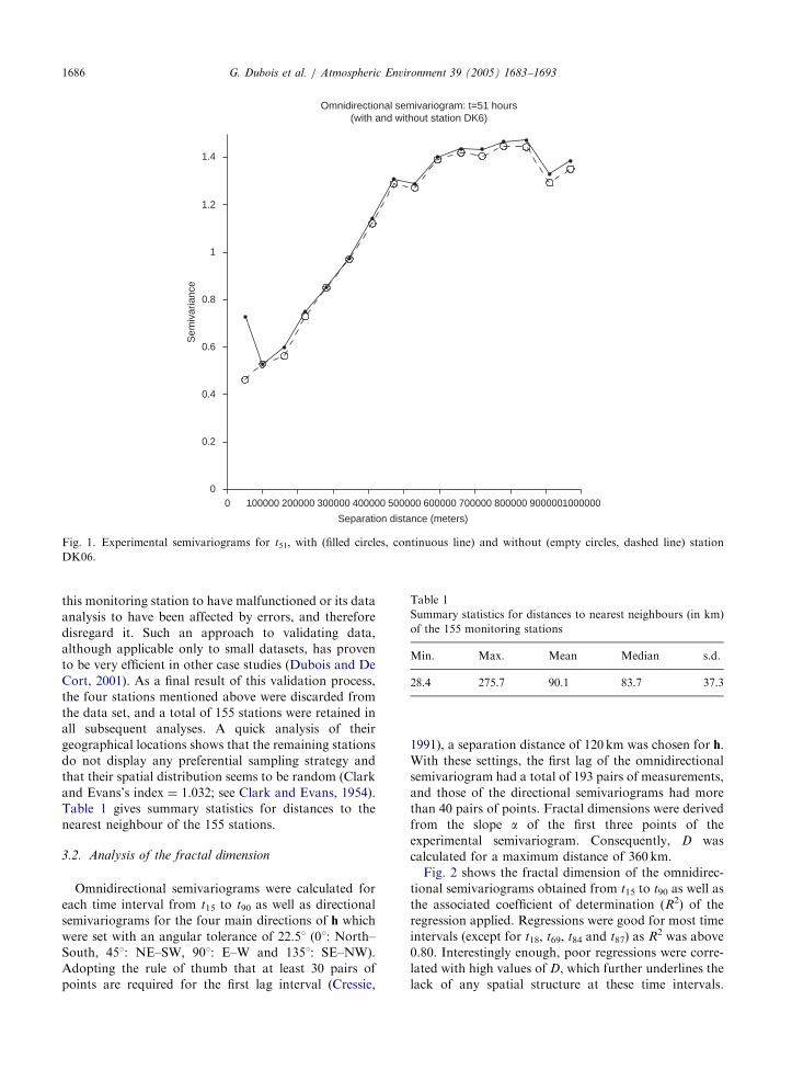
lands, have the codes F04, F16, DK06 and NL06. Fig. 1

shows an example of the impact of such outliers on the

experimental semivariogram for t51: DK06 systemati-

cally increases the semivariance at short distances. As

expected, if we remove this station from the dataset, the

semivariance drops and becomes more consistent with

the trend of the other points. Since the effect of DK06

on the semivariogram shown in Fig. 1 also occurred for

different time intervals, we could reasonably consider

ARTICLE IN PRESS

Table 1

Summary statistics for distances to nearest neighbours (in km)

of the 155 monitoring stations

Min. Max. Mean Median s.d.

28.4 275.7 90.1 83.7 37.3

0 100000 200000 300000 400000 500000 600000 700000 800000 9000001000000

Separation distance (meters)

0

0.2

0.4

0.6

0.8

1

1.2

1.4

Sem

ivar

ianc

e

Omnidirectional semivariogram: t=51 hours(with and without station DK6)

Fig. 1. Experimental semivariograms for t51, with (filled circles, continuous line) and without (empty circles, dashed line) station

DK06.

G. Dubois et al. / Atmospheric Environment 39 (2005) 1683–16931686

this monitoring station to have malfunctioned or its data

analysis to have been affected by errors, and therefore

disregard it. Such an approach to validating data,

although applicable only to small datasets, has proven

to be very efficient in other case studies (Dubois and De

Cort, 2001). As a final result of this validation process,

the four stations mentioned above were discarded from

the data set, and a total of 155 stations were retained in

all subsequent analyses. A quick analysis of their

geographical locations shows that the remaining stations

do not display any preferential sampling strategy and

that their spatial distribution seems to be random (Clark

and Evans’s index ¼ 1.032; see Clark and Evans, 1954).

Table 1 gives summary statistics for distances to the

nearest neighbour of the 155 stations.

3.2. Analysis of the fractal dimension

Omnidirectional semivariograms were calculated for

each time interval from t15 to t90 as well as directional

semivariograms for the four main directions of h which

were set with an angular tolerance of 22.51 (01: North–

South, 451: NE–SW, 901: E–W and 1351: SE–NW).

Adopting the rule of thumb that at least 30 pairs of

points are required for the first lag interval (Cressie,

1991), a separation distance of 120 km was chosen for h.

With these settings, the first lag of the omnidirectional

semivariogram had a total of 193 pairs of measurements,

and those of the directional semivariograms had more

than 40 pairs of points. Fractal dimensions were derived

from the slope a of the first three points of the

experimental semivariogram. Consequently, D was

calculated for a maximum distance of 360 km.

Fig. 2 shows the fractal dimension of the omnidirec-

tional semivariograms obtained from t15 to t90 as well as

the associated coefficient of determination (R2) of the

regression applied. Regressions were good for most time

intervals (except for t18, t69, t84 and t87) as R2 was above

0.80. Interestingly enough, poor regressions were corre-

lated with high values of D, which further underlines the

lack of any spatial structure at these time intervals.

ARTICLE IN PRESS

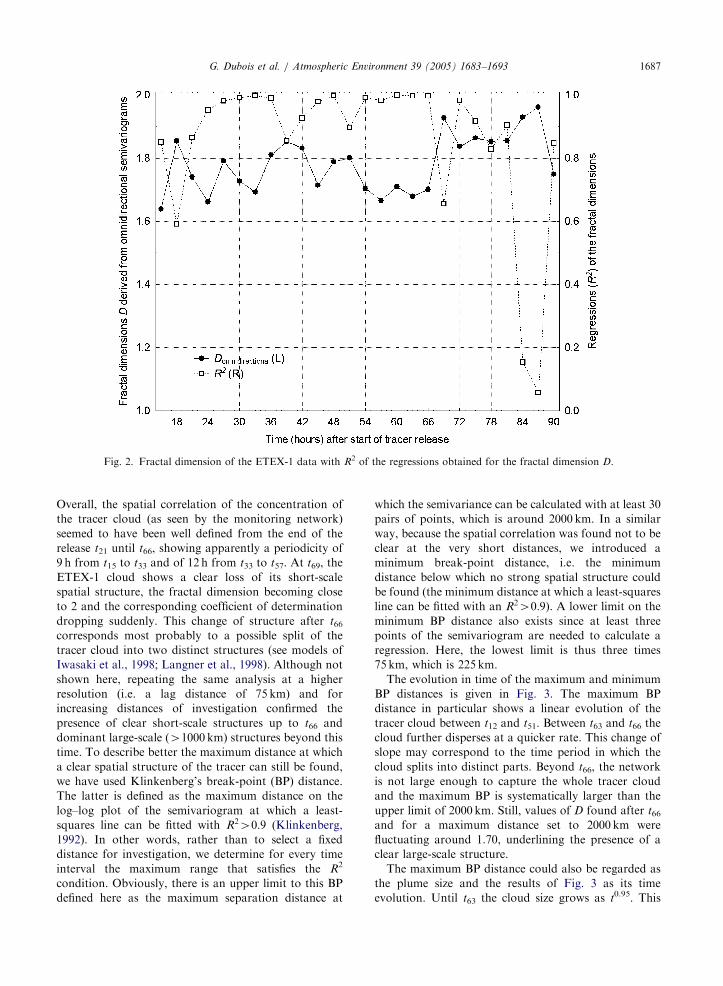
Fig. 2. Fractal dimension of the ETEX-1 data with R2 of the regressions obtained for the fractal dimension D.

G. Dubois et al. / Atmospheric Environment 39 (2005) 1683–1693 1687

Overall, the spatial correlation of the concentration of

the tracer cloud (as seen by the monitoring network)

seemed to have been well defined from the end of the

release t21 until t66, showing apparently a periodicity of

9 h from t15 to t33 and of 12 h from t33 to t57. At t69, the

ETEX-1 cloud shows a clear loss of its short-scale

spatial structure, the fractal dimension becoming close

to 2 and the corresponding coefficient of determination

dropping suddenly. This change of structure after t66corresponds most probably to a possible split of the

tracer cloud into two distinct structures (see models of

Iwasaki et al., 1998; Langner et al., 1998). Although not

shown here, repeating the same analysis at a higher

resolution (i.e. a lag distance of 75 km) and for

increasing distances of investigation confirmed the

presence of clear short-scale structures up to t66 and

dominant large-scale (41000 km) structures beyond thistime. To describe better the maximum distance at which

a clear spatial structure of the tracer can still be found,

we have used Klinkenberg’s break-point (BP) distance.

The latter is defined as the maximum distance on the

log–log plot of the semivariogram at which a least-

squares line can be fitted with R240:9 (Klinkenberg,1992). In other words, rather than to select a fixed

distance for investigation, we determine for every time

interval the maximum range that satisfies the R2

condition. Obviously, there is an upper limit to this BP

defined here as the maximum separation distance at

which the semivariance can be calculated with at least 30

pairs of points, which is around 2000 km. In a similar

way, because the spatial correlation was found not to be

clear at the very short distances, we introduced a

minimum break-point distance, i.e. the minimum

distance below which no strong spatial structure could

be found (the minimum distance at which a least-squares

line can be fitted with an R240:9). A lower limit on theminimum BP distance also exists since at least three

points of the semivariogram are needed to calculate a

regression. Here, the lowest limit is thus three times

75 km, which is 225 km.

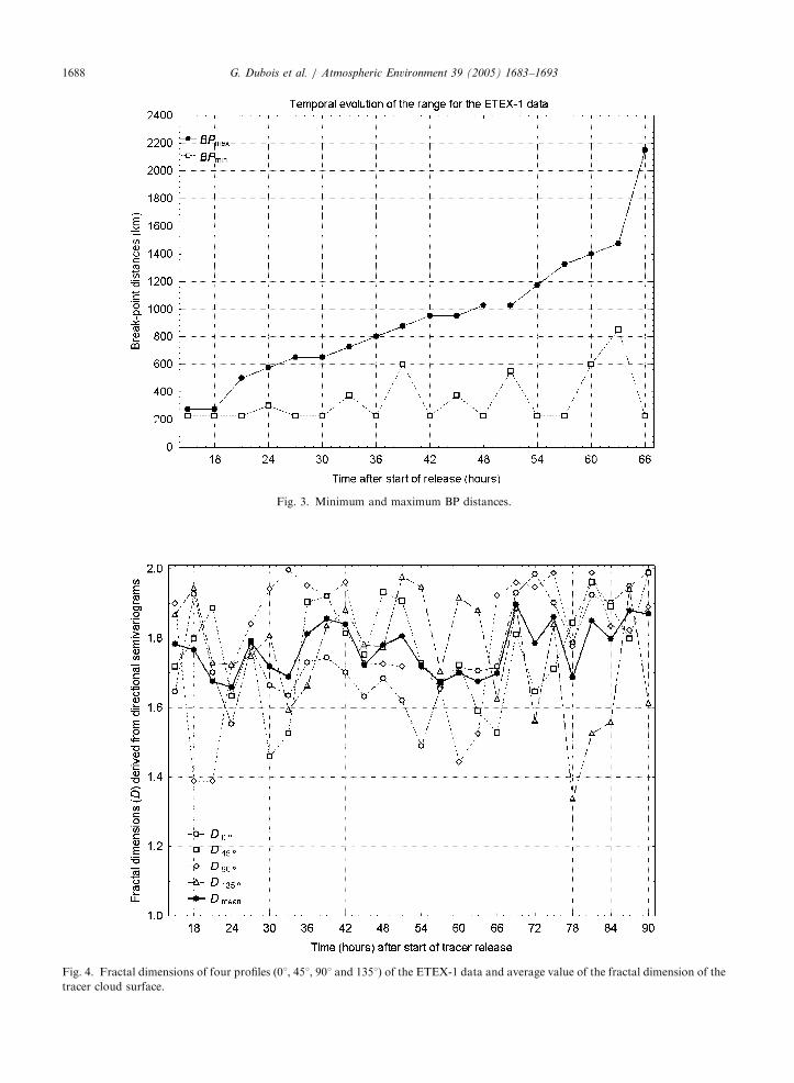
The evolution in time of the maximum and minimum

BP distances is given in Fig. 3. The maximum BP

distance in particular shows a linear evolution of the

tracer cloud between t12 and t51. Between t63 and t66 the

cloud further disperses at a quicker rate. This change of

slope may correspond to the time period in which the

cloud splits into distinct parts. Beyond t66, the network

is not large enough to capture the whole tracer cloud

and the maximum BP is systematically larger than the

upper limit of 2000 km. Still, values of D found after t66and for a maximum distance set to 2000 km were

fluctuating around 1.70, underlining the presence of a

clear large-scale structure.

The maximum BP distance could also be regarded as

the plume size and the results of Fig. 3 as its time

evolution. Until t63 the cloud size grows as t0.95. This

ARTICLE IN PRESS

Fig. 3. Minimum and maximum BP distances.

Fig. 4. Fractal dimensions of four profiles (01, 451, 901 and 1351) of the ETEX-1 data and average value of the fractal dimension of the

tracer cloud surface.

G. Dubois et al. / Atmospheric Environment 39 (2005) 1683–16931688

ARTICLE IN PRESSG. Dubois et al. / Atmospheric Environment 39 (2005) 1683–1693 1689

exponent lies in the range between 0.5 and 1, which

agrees well with predictions from classical dispersion

theory (the analysis, nevertheless, does not allow us to

distinguish between later dispersion and transport

direction). This result gives strong indications that the

network performed well in capturing the physical

phenomenon until the cloud split. For what concerns

the minimum values of the BP, we will limit

our comments to mentioning the periodic loss of the

short-scale spatial correlation until the end of the

experiment (t90).

The clear diffusion process of the tracer cloud

described above should be further confirmed by the

presence of unambiguous anisotropies. By looking at the

cloud by means of four ‘‘transects’’ oriented in the four

main directions, one will find very different spatial

structures as shown by their respective fractal dimen-

sions in Fig. 4. These differences underline the rapid

Fig. 5. Evolution in time (t15 to t66) of the main

fluctuation in time of the spatial structures and thus the

effect of the transport and dispersion in different

directions of the core structure of the tracer cloud.

Fig. 4 also shows the fractal dimension obtained by

averaging the ones obtained for the four transects. By

comparing this last curve with the fractal dimensions

derived from the omnidirectional semivariograms as

shown in Fig. 2, one can find an exact correspondence

from t24 until t75 (R2 ¼ 0:96).

To investigate more in detail the temporal evolution

of the spatial anisotropies of the ETEX-1 data,

semivariogram maps were also used. These maps are

grids that show the semivariance for different separation

distances in every direction. Instead of comparing

different directional semivariograms, one can in such

a way easily detect anisotropies in a single map by

identifying directions for which the semivariance is lower

(Deutsch and Journel, 1992; Pannatier, 1996). Fig. 5

orientation of the ETEX-1 tracer cloud.

ARTICLE IN PRESS

0 100 200 300 400 500 600Lag distance (km)

0

0.2

0.4

0.6

0.8

1

1.2

= 0.01

= 0.05

= 0.1

= 0.5

Concentration thresholds (ng/m3)

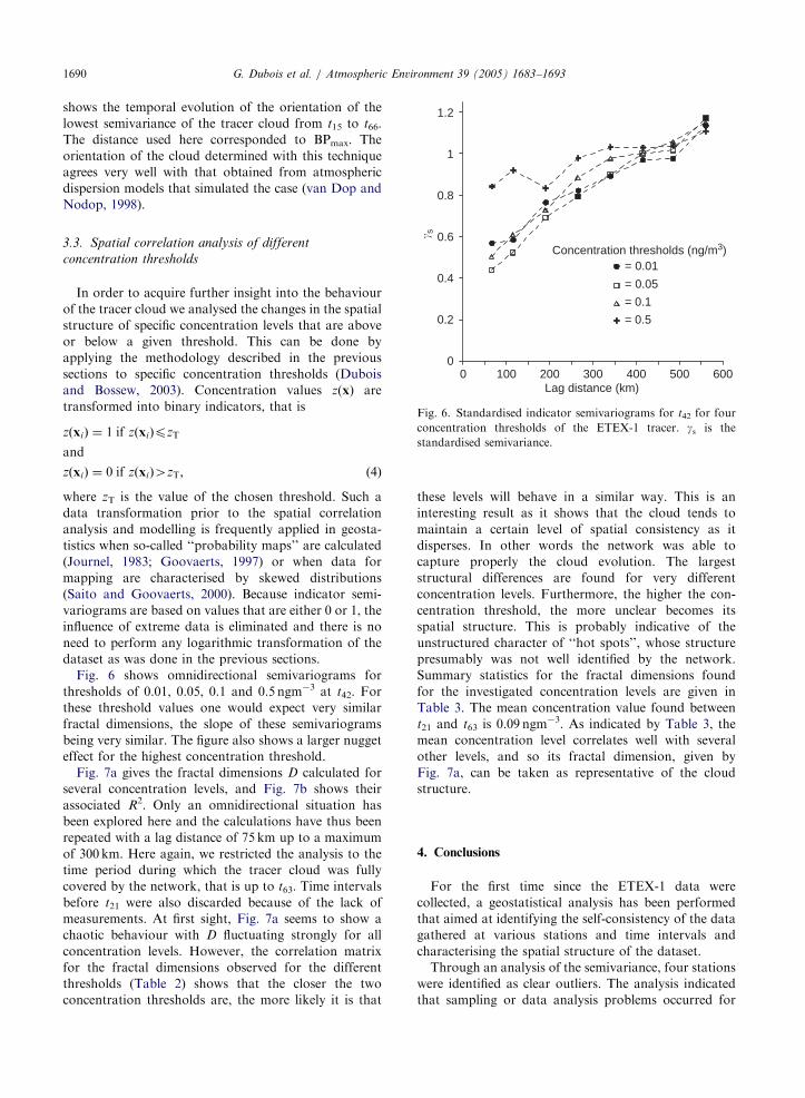
� sFig. 6. Standardised indicator semivariograms for t42 for four

concentration thresholds of the ETEX-1 tracer. gs is thestandardised semivariance.

G. Dubois et al. / Atmospheric Environment 39 (2005) 1683–16931690

shows the temporal evolution of the orientation of the

lowest semivariance of the tracer cloud from t15 to t66.

The distance used here corresponded to BPmax. The

orientation of the cloud determined with this technique

agrees very well with that obtained from atmospheric

dispersion models that simulated the case (van Dop and

Nodop, 1998).

3.3. Spatial correlation analysis of different

concentration thresholds

In order to acquire further insight into the behaviour

of the tracer cloud we analysed the changes in the spatial

structure of specific concentration levels that are above

or below a given threshold. This can be done by

applying the methodology described in the previous

sections to specific concentration thresholds (Dubois

and Bossew, 2003). Concentration values z(x) are

transformed into binary indicators, that is

zðxiÞ ¼ 1 if zðxiÞpzT

and

zðxiÞ ¼ 0 if zðxiÞ4zT; ð4Þ

where zT is the value of the chosen threshold. Such a

data transformation prior to the spatial correlation

analysis and modelling is frequently applied in geosta-

tistics when so-called ‘‘probability maps’’ are calculated

(Journel, 1983; Goovaerts, 1997) or when data for

mapping are characterised by skewed distributions

(Saito and Goovaerts, 2000). Because indicator semi-

variograms are based on values that are either 0 or 1, the

influence of extreme data is eliminated and there is no

need to perform any logarithmic transformation of the

dataset as was done in the previous sections.

Fig. 6 shows omnidirectional semivariograms for

thresholds of 0.01, 0.05, 0.1 and 0.5 ngm�3 at t42. For

these threshold values one would expect very similar

fractal dimensions, the slope of these semivariograms

being very similar. The figure also shows a larger nugget

effect for the highest concentration threshold.

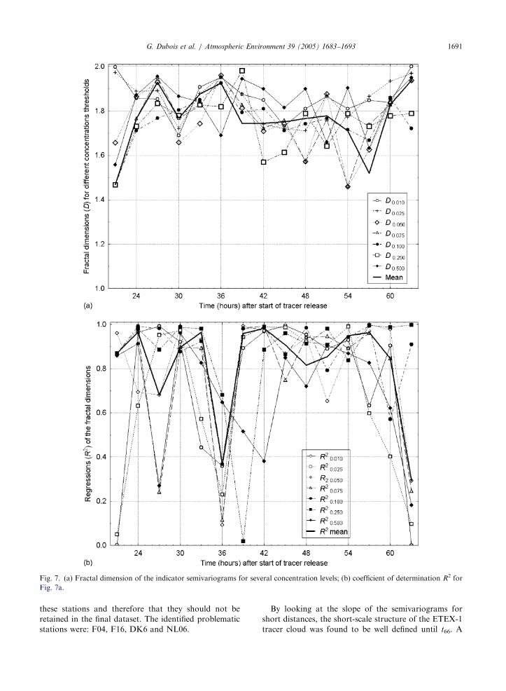
Fig. 7a gives the fractal dimensions D calculated for

several concentration levels, and Fig. 7b shows their

associated R2. Only an omnidirectional situation has

been explored here and the calculations have thus been

repeated with a lag distance of 75 km up to a maximum

of 300 km. Here again, we restricted the analysis to the

time period during which the tracer cloud was fully

covered by the network, that is up to t63. Time intervals

before t21 were also discarded because of the lack of

measurements. At first sight, Fig. 7a seems to show a

chaotic behaviour with D fluctuating strongly for all

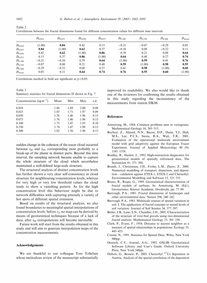
concentration levels. However, the correlation matrix

for the fractal dimensions observed for the different

thresholds (Table 2) shows that the closer the two

concentration thresholds are, the more likely it is that

these levels will behave in a similar way. This is an

interesting result as it shows that the cloud tends to

maintain a certain level of spatial consistency as it

disperses. In other words the network was able to

capture properly the cloud evolution. The largest

structural differences are found for very different

concentration levels. Furthermore, the higher the con-

centration threshold, the more unclear becomes its

spatial structure. This is probably indicative of the

unstructured character of ‘‘hot spots’’, whose structure

presumably was not well identified by the network.

Summary statistics for the fractal dimensions found

for the investigated concentration levels are given in

Table 3. The mean concentration value found between

t21 and t63 is 0.09 ngm�3. As indicated by Table 3, the

mean concentration level correlates well with several

other levels, and so its fractal dimension, given by

Fig. 7a, can be taken as representative of the cloud

structure.

4. Conclusions

For the first time since the ETEX-1 data were

collected, a geostatistical analysis has been performed

that aimed at identifying the self-consistency of the data

gathered at various stations and time intervals and

characterising the spatial structure of the dataset.

Through an analysis of the semivariance, four stations

were identified as clear outliers. The analysis indicated

that sampling or data analysis problems occurred for

ARTICLE IN PRESS

Fig. 7. (a) Fractal dimension of the indicator semivariograms for several concentration levels; (b) coefficient of determination R2 for

Fig. 7a.

G. Dubois et al. / Atmospheric Environment 39 (2005) 1683–1693 1691

these stations and therefore that they should not be

retained in the final dataset. The identified problematic

stations were: F04, F16, DK6 and NL06.

By looking at the slope of the semivariograms for

short distances, the short-scale structure of the ETEX-1

tracer cloud was found to be well defined until t66. A

ARTICLE IN PRESS

Table 2

Correlations between the fractal dimensions found for different concentration values for different time intervals

D0.010 D0.025 D0.050 D0.075 D0.100 D0.250 D0.500 Dmean

D0.010 (1.00) 0.84 0.42 0.15 �0.21 �0.07 �0.29 0.05

D0.025 0.84 (1.00) 0.62 0.37 �0.10 0.08 �0.32 0.11

D0.050 0.42 0.62 (1.00) 0.86 0.39 0.21 0.08 0.64

D0.075 0.15 0.37 0.86 (1.00) 0.64 0.48 0.27 0.74

D0.100 �0.21 �0.10 0.39 0.64 (1.00) 0.59 0.41 0.76

D0.250 �0.07 0.08 0.21 0.48 0.59 (1.00) 0.58 0.55

D0.500 �0.29 �0.32 0.08 0.27 0.41 0.58 (1.00) 0.60

Dmean 0.05 0.11 0.64 0.74 0.76 0.55 0.60 (1.00)

Correlations marked in bold are significant at po0.05.

Table 3

Summary statistics for fractal dimensions D shown in Fig. 7

Concentrations (ngm�3) Mean Min. Max. s.d.

0.010 1.86 1.69 2.00 0.08

0.025 1.85 1.71 1.97 0.09

0.050 1.76 1.46 1.96 0.15

0.075 1.76 1.46 1.96 0.15

0.100 1.75 1.47 1.93 0.10

0.250 1.74 1.47 1.98 0.13

0.500 1.82 1.56 1.96 0.13

G. Dubois et al. / Atmospheric Environment 39 (2005) 1683–16931692

sudden change in the cohesion of the tracer cloud occurred

between t66 and t69, corresponding most probably to a

break-up of the plume in distinct parts. Beyond this time

interval, the sampling network became unable to capture

the whole structure of the cloud which nevertheless

maintained a well-defined large-scale structure.

The structural analysis of distinct concentration levels

has further shown a very clear self-consistency in cloud

structure for neighbouring concentration levels, whereas

for very high or very low threshold values the cloud

tends to show a vanishing pattern. As for the high

concentration level this behaviour might be due to

network difficulties with capturing precisely a variety of

hot spots of different spatial extension.

Based on results of the structural analysis, we also

found boundaries to meaningful spatial interpolations of

concentration levels: before t21 no map can be derived by

means of geostatistical techniques because of a lack of

data; after t66 extrapolations will become inevitable.

Future work will start from the results obtained in this

study and will aim to generate interpolation maps of the

concentration measurements.

Acknowledgements

We are thankful to our colleague Tore Tollefsen

whose meticulous review of the manuscript substantially

improved its readability. We also would like to thank

one of the reviewers for confirming the results obtained

in this study regarding the inconsistency of the

measurements from station DK06.

References

Armstrong, M., 1984. Common problems seen in variograms.

Mathematical Geology 16, 305–313.

Boybeyi, Z., Ahmad, N.N., Bacon, D.P., Dunn, T.J., Hall,

M.S., Lee, P.C.S., Sarna, R.A., Wait, T.R., 2001.

Evaluation of the operational multiscale environment

model with grid adaptivity against the European Tracer

Experiment. Journal of Applied Meteorology 40 (9),

1541–1558.

Bradley, R., Haslett, J., 1992. High-interaction diagnostics for

geostatistical models of spatially referenced data. The

Statistician 41, 371–380.

Brandt, J., Christensen, J.H., Frohn, L.M., Zlatev, Z., 2000.

Numerical modelling of transport, dispersion, and deposi-

tion—validation against ETEX-1, ETEX-2 and Chernobyl.

Environmental Modelling and Software 15, 521–531.

Bruno, R., Raspa, G., 1989. Geostatistical characterization of

fractal models of surfaces. In: Armstrong, M. (Ed.),

Geostatistics. Kluwer Academic, Dordrecht, pp. 77–89.

Burrough, P.A., 1981. Fractal dimensions of landscapes and

other environmental data. Nature 294, 240–242.

Burrough, P.A., 1983. Multiscale sources of spatial variation in

soil. I. The application of fractal concepts to nested levels of

soil variation. Journal of Soil Science 34, 577–597.

Butler, J.B., Lane, S.N., Chandler, J.H., 2001. Characterization

of the structure of river-bed gravels using two-dimensional

fractal analysis. Mathematical Geology 33, 301–330.

Clark, P., Evans, F., 1954. Distance to nearest neighbor as a

measure of spatial relationships in populations. Ecology 35,

445–453.

Cressie, N., 1991. Statistics for Spatial Data. Wiley, New York

900pp.

Deutsch, C.V., Journel, A.G., 1992. GSLIB: Geostatistical

Software Library and User’s Guide. Oxford University

Press, New York 340pp.

Dubois, G., Bossew, P., 2003. Chernobyl 137Cs deposition in

Austria. Analysis of the spatial correlation of the deposition

ARTICLE IN PRESSG. Dubois et al. / Atmospheric Environment 39 (2005) 1683–1693 1693

levels. Journal of Environmental Radioactivity 65 (1),

29–45.

Dubois, G., De Cort, M., 2001. Mapping 137Cs: data validation

methods and data interpretation. Journal of Environmental

Radioactivity 53 (3), 271–289.

Galmarini, S., Bianconi, R., Addis, R., Andronopoulos, S.,

Astrup, P., Bartzis, J.C., Bellasio, R., Buckley, R.,

Champion, H., Chino, M., D’Amours, R., Davakis, E.,

Eleveld, H., Glaab, H., Manning, A., Mikkelsen, T.,

Pechinger, U., Polreich, E., Prodanova, M., Slaper, H.,

Syrakov, D., Terada, H., Van der Auwera, L., 2004.

Ensemble dispersion forecasting, part II: application and

evaluation. Atmospheric Environment 38 (28), 4619–4632.

Girardi, F., Graziani, G., van Veltzen, D., Galmarini, S., Mosca, S.,

Bianconi, R., Bellasio, R., Klug, W. (Eds.), 1998. The ETEX

project. EUR Report 18143 EN. Office for Official Publications

of the European Communities, Luxembourg, 108pp.

Goovaerts, P., 1997. Geostatistics for Natural Resources

Evaluation. Oxford University Press, New York 467pp.

Graziani, G., Mosca, S., Klug, W., 1998a. Real-time long-range

dispersion model evaluation of ETEX first release. EUR

Report 17754 EN. Office for Official Publications of the

European Communities, Luxembourg.

Graziani, G., Klug, W., Galmarini, S., Grippa, G., 1998b. Real-

time long-range dispersion model evaluation of ETEX

second release. EUR 17755 EN. Office for Official Publica-

tions of the European Communities, Luxembourg.

Gringarten, E., Deutsch, C., 2001. Variogram interpretation

and modeling. Mathematical Geology 33, 507–534.

Haslett, J., Bradley, R., Craig, P., Unwin, A., Wills, G., 1991.

Dynamic graphics for exploring spatial data with applica-

tion to locating global and local anomalies. The American

Statistician 45, 234–242.

Iwasaki, T., Maki, T., Katayama, K., 1998. Tracer transport

model at Japan meteorological agency and its application to

the ETEX data. Atmospheric Environment 32 (24),

4285–4295.

Journel, A.G., 1983. Nonparametric estimation of spatial

distributions. Mathematical Geology 15, 445–468.

Journel, A.G., Huijbregts, C.J., 1978. Mining Geostatistics.

Academic Press, London 500pp.

Klinkenberg, B., 1992. Fractals and morphometric measures: is

there a relationship? Geomorphology 5, 5–20.

Kovalets, I., Andronopoulos, S., Bartzis, J.G., Gounaris, N.,

Kushchan, A., 2004. Introduction of data assimilation

procedures in the meteorological pre-processor of atmo-

spheric dispersion models used in emergency response

systems. Atmospheric Environment 38, 457–467.

Lam, N.S., 1983. Spatial interpolation methods: a review. The

American Cartographer 10, 129–149.

Langner, J., Robertson, L., Persson, C., Ullerstig, A., 1998.

Validation of the operational emergency response model at

the Swedish Meteorological and Hydrological Institute

using data from ETEX and the Chernobyl accident.

Atmospheric Environment 32, 4325–4333.

Matheron, G., 1963. Principles of Geostatistics. Economic

Geology 58, 1246–1266.

Matheron, G., 1971. The theory of regionalised variables and

its applications. Cahier No. 5, Centre de Morphologie

Mathematique de Fontainebleau, Ecole Superieure des

Mines de Paris. 211pp.

Pannatier, Y., 1996. VARIOWIN: Software for Spatial Data

Analysis in 2D. Springer, New York 91pp.

Saito, H., Goovaerts, P., 2000. Geostatistical interpolation of

positively skewed and censored data in a dioxin-contami-

nated site. Environmental Science and Technology 34,

4228–4235.

Schwere, S., Stohl, A., Rotach, M.W., 2002. Practical

considerations to speed up Lagrangian stochastic particle

models. Computers and Geosciences 28, 143–154.

Van Dop, H., Nodop, K., 1998. ETEX: a European

tracer experiment. Atmospheric Environment 32,

4089–4378.

Van Dop, H., Addis, R., Fraser, G., Girardi, F., Graziani, G.,

Inoue, Y., Kelly, N., Klug, W., Kulmala, A., Nodop, K.,

Pretel, J., 1998. ETEX: a European tracer experiment;

observations, dispersion modelling and emergency response.

Atmospheric Environment 32, 4089–4094.

Warner, S., Platt, N., Heagy, J.F., 2003. Application of user-

oriented MOE to transport and dispersion model predic-

tions of the European tracer experiment. IDA Paper P-3829,

Institute for Defense Analyses, Alexandria, VA.

Yang, Z.Y., Di, C.C., 2001. A directional method for directly

calculating the fractal parameters of joint surface roughness.

International Journal of Rock Mechanics and Mining

Sciences 38, 1201–1210.