Geostatistical analysis of health data with different levels of spatial aggregation

Spatial and Spatio-temporal Epidemiology 3 (2012) 83–92

Contents lists available at SciVerse ScienceDirect

Spatial and Spatio-temporal Epidemiology

journal homepage: www.elsevier .com/locate /sste

Geostatistical analysis of health data with different levelsof spatial aggregation

Pierre Goovaerts ⇑BioMedware Inc., 3526 W Liberty, Suite 100, Ann Arbor, Michigan 48103, USA

a r t i c l e i n f o

Article history:Available online 11 February 2012

Keywords:Prostate cancerCensus tractBinomial krigingLate-stage diagnosisFlorida

1877-5845/$ - see front matter � 2012 Elsevier Ltddoi:10.1016/j.sste.2012.02.008

⇑ Tel.: +1 734 913 1098; fax: +1 734 913 2201.E-mail address: [email protected]

a b s t r a c t

This paper presents a geostatistical approach to combine two geographical sets of area-based data into the mapping of disease risk, with an application to the rate of prostate cancerlate-stage diagnosis in North Florida. This methodology is used to combine individual-leveldata assigned to census tracts for confidentiality reasons with individual-level data thatwere allocated to ZIP codes because of incomplete geocoding. This form of binomialkriging, which accounts for the population size and shape of each geographical unit, cangenerate choropleth or isopleth risk maps that are all coherent through spatial aggregation.Incorporation of both types of areal data reduces the loss of information associated withincomplete geocoding, leading to maps of risk estimates that are globally less smoothand with smaller prediction error variance.

� 2012 Elsevier Ltd. All rights reserved.

1. Introduction

For cancer control activities and resource allocation, it isimportant to be able to compare incidence and survivalrates, risk behaviors, screening patterns, diagnosis stage,and treatment methods across geographical and politicalboundaries and at as fine a spatial scale as possible. Withthe proliferation of geographic information systems (GIS)and related databases, it is becoming easier to gather infor-mation at the individual-level. The assignment of a set ofspatial coordinates (geocode) to subjects’ residences is thecornerstone of any analysis of individual-level health data.Direct measurement of these coordinates is rare andresearchers rely on cheaper geocoding methods, such asidentification on orthophoto maps, address matching to adigital street map (automatic geocoding) or the local 911listing (Rushton et al., 2006).

According to several studies (Cayo and Talbot, 2003;Ward et al., 2005; Strickland et al., 2007; Zimmermanand Li, 2010) the magnitude of geocoding errors can besubstantial, up to several hundred meters and even more

. All rights reserved.

in rural areas where longer street segments and unevenspacing between houses increase interpolation errors whenplacing an address based on the street numbers assigned tothe ends of each street segment. E911 geocodes are moreaccurate but still not available everywhere. Uncertaintyabout the exact location of a residence can also result fromthe aggregation or randomization performed on the result-ing point to protect the identity of the geocoded object,which is often the case in the geocoding of health data(Goldberg et al., 2007; Wieland et al., 2008). These geocod-ing errors frequently hamper the statistical analysis ofcancer data by reducing the power to detect cancer clus-ters (Zimmerman, 2008a; Jacquez and Rommel, 2009),the ability to identify relationships with geographicallyvarying risk factors (Mazumdar et al., 2008), and theaccuracy of fine-level cancer maps (Zimmerman, 2008b).

In addition to the uncertainty attached to the residencecoordinates, addresses can fail to geocode. Indeed, the geo-coding process is extraordinarily complex and many prob-lems can affect either the residential address (e.g. spellingerrors, post office box addresses, street suffix, prefix andabbreviation inconsistencies) or the reference files thatcan contain errors such as missing, incomplete, and incor-rect street segments and address ranges. The end results

84 P. Goovaerts / Spatial and Spatio-temporal Epidemiology 3 (2012) 83–92

are missing or incomplete data where coarser surrogates,such as ZIP code, replace precise coordinates. The percent-age of incomplete geocoding tends to increase for casesdiagnosed several decades ago (Han et al., 2005), whichhampers the characterization of temporal trends in healthoutcomes and the assessment of the benefits of preventionand control strategies to reduce cancer burden.

Since rural addresses are less likely to be successfullygeocoded, a straightforward exclusion of incomplete datacould lead to geographic selection bias and misleading re-sults (Rushton et al., 2006). Simply assigning the data tothe geographical or population-weighted centroid of theZIP code is also unsatisfactory because this point could fallinto inhabited areas and it is a crude estimate for large ZIPcodes (Hibbert et al., 2009). One common way to handleincomplete data is through geographic imputation where-by latitude and longitude coordinates or some other appro-priate geographic identifier are assigned to nongeocodedaddresses (e.g. Klassen et al., 2005; Henry and Boscoe,2008; Curriero et al., 2010). For example, Hibbert et al.(2009) compared the accuracy of eight deterministic andstochastic geo-imputation methods to allocate cases of dia-betes from zip codes to census tracts. The allocation wasbased on either the land area or the population demo-graphics (total population, population under 19, and race/ethnicity). They found that the imputation approachshould be selected according to the study aims since deter-ministic approaches yield greater accuracy at the individuallevel (i.e. greater percentage of cases allocated correctly toa tract), whereas stochastic methods better reproduce thetrue spatial distribution of cases (greater group levelaccuracy).

Although geo-imputation methods are easily imple-mented within GIS and a measure of uncertainty can becomputed for the imputed counts (Curriero et al., 2010),such an approach does not address the issue of rates insta-bility in sparsely sampled areas and the limitations associ-ated with the interpretation of choropleth maps when theuser tends to assign more importance to larger polygonsalthough they typically correspond to rural areas withsmaller populations at risk. These effects are particularlyimportant for census tracts since they typically display awide range of sizes and shapes. The geostatistical approachadopted in this paper falls within the areas of change ofsupport (Gotway and Young, 2002) and disease mapping(Waller and Gotway, 2004). Areal data defined over differ-ent spatial supports are interpolated to a fine grid in orderto map the underlying risk of developing the disease as acontinuous surface.

Zimmerman and Fang (in press) recently demonstratedthrough simulation studies that using coarsened data im-proves substantially the accuracy of the maps of risk esti-mates relative to prediction based only on observationsthat were successfully geocoded. Their nonparametriccoarsened-data methodology was very straightforward,both conceptually and computationally, yet no measureof prediction accuracy was provided and the approach as-sumes that geocoding errors were negligible. This latterassumption was also inherent to the geostatistical ap-proach proposed by Goovaerts (2009) to incorporate bothpoint and areal data in the mapping of health outcomes.

This kriging technique however provides a measure ofthe variance of prediction errors and its recent generaliza-tion as ‘‘Area-and-Point kriging’’ (Goovaerts, 2010) allowsthe mapping of attribute values within each sampled geo-graphical unit under the constraint that the average of pointestimates returns the areal data (coherency constraint).

The kriging approach accounts for the shape and size ofgeographical units, hence it can accommodate differentspatial supports for the data and the prediction, and it isnot restricted to a single type of areal data at a time (e.g.ZIP code or census tracts). For example, Gotway and Young(2007) used kriging for mapping the number of low birthweight (LBW) babies at the census tract-level, accountingfor county-level LBW data and covariates measured overdifferent spatial supports, such as a fine grid of ground-le-vel particulate matter concentrations or tract population.Such flexibility is needed when geocoded data are eitherunreliable or were randomized for confidentiality reasons(Hampton et al., 2010), making their spatial aggregationdesirable before proceeding with any analysis.

This paper presents a geostatistical approach to com-bine two geographical sets of area-based data into themapping of health outcomes. This form of binomial kriging(Goovaerts, 2009), which accounts for the population sizeand shape of each geographical unit, can generate choro-pleth or isopleth risk maps that are coherent with thenoise-filtered areal data (i.e. return the areal data throughspatial aggregation). This methodology is here used tocombine two types of areal data in the isopleth mappingof the percentage of prostate cancer that were diagnosedlate across 25 counties of Florida: (1) census tract-levelrates computed from geocoded data that were randomizedwithin each tract for confidentiality reasons, and (2) ZIPcode-level rates calculated using all records, includingthe ones that failed to geocode. The impact of incorporat-ing the two types of data is illustrated by comparison tothe results obtained using area-to-area and area-to-pointkriging (Kyriakidis, 2004; Goovaerts, 2006) based only onZIP code data.

2. Data and methods

2.1. Prostate cancer data

The geostatistical mapping approach will be illustratedusing prostate cancer cases who were diagnosed duringthe calendar years 1981 through 2008 in Florida. The anal-ysis will be restricted to non-Hispanic white males aged40 years or older. Approximately 7.3% of the 293,651 re-cords, which were compiled by the Florida Cancer DataSystem (FCDS) and processed by an independent geocod-ing firm, were not successfully geocoded at residence attime of diagnosis. This percentage however greatly varieswith time and space. Fig. 1A show that incomplete geocod-ing is more likely for earlier years of diagnosis: on averageover Florida the percentage decreases from 23% in 1981 to3.12% in 2008. This percentage is also greater for countiesclassified as non-metropolitan (non-metro) on the basisof the US Department of Agriculture Rural–Urban ContinuumCodes (USDA, 2004). This nine-part county codification

Fig. 1. Temporal change in the percentage of prostate cancer cases that failed to geocode on average over Florida and for metropolitan versus non-metropolitan counties (A). The bottom map shows the county-level percentage of incomplete geocoding averaged over the period 1981–2008 (B). Thickwhite borders highlight the subset of 25 counties used for the geostatistical analysis.

P. Goovaerts / Spatial and Spatio-temporal Epidemiology 3 (2012) 83–92 85

distinguishes metro counties by the population size oftheir metro area, and non-metro counties by degree ofurbanization and adjacency to a metro area or areas. Thisinformation was available for 1983, 1993 and 2003. For1983 and 1993 codes 0 and 1 were combined to makethese classifications comparable to the 20030s codification.These codes were linearly interpolated over the periods1983–1993 and 1993–2003.

Discrepancies between both metro and non-metrocounties were particularly large in the early 19s whenthe introduction of PSA screening caused a surge in the

number of diagnosed cases. The frequency of incompletegeocoding was then more than four times larger for casesdiagnosed in non-metro counties (Fig. 1A). This greaterlikelihood for rural addresses to be unsuccessfully geocod-ed has been well documented and is caused by variousfactors, such as disproportionate number of rural routeaddresses, post office box addresses, unofficial streetnames and streets missing from geocoding reference files(Whitsel et al., 2006; Kravets and Hadden, 2007). Thecounty-level map of time averaged percentage of incom-plete geocoding (Fig. 1B) reveals substantial geographical

86 P. Goovaerts / Spatial and Spatio-temporal Epidemiology 3 (2012) 83–92

disparities that go beyond the dichotomy between metro-politan and non-metropolitan counties. Except for twoSouthern counties that include the Florida key Islands(Monroe County) and part of the Everglades (GladesCounty), most geocoding problems occurred in NorthernFlorida, in particular in the Panhandle.

The 21,365 incomplete records were assigned to theirZIP code centroids, whereas the geographical coordinatesof the geocoded records were randomized within each cen-sus tract for confidentiality reasons. Data thus exist overtwo overlapping and non-nested sets of geographicalunits: ZIP codes and census tracts.

The present study will focus on 25 counties of NorthernFlorida where the largest percentage of incomplete geo-coding was recorded and that are highlighted using thickwhite borders in Fig. 1B. This region (Fig. 2A) includesthe centroids of 273 ZIP codes (Fig. 2B) and 222 censustracts (Fig. 2C) that form the two geographies availablefor mapping the percentage of late-stage diagnosis. Withinthese 25 counties 7958 patients had their residence geo-coded whereas 1666 records were incomplete. The spa-tio-temporal analysis of health data aggregated at the ZIPcode-level is challenging since the definition of these geo-graphical units changes with time (Krieger et al., 2002) andshape files with ZIP code boundaries are not readily avail-able prior to 2000. In addition, USPS ZIP codes representpostal delivery routes without true geographic boundaries.Since this paper is primarily concerned with the develop-ment of a new methodology instead of a detailed analysisof prostate cancer late-stage diagnosis in Florida, the ZIPcode geography was simply based on the shape file of ZIPCode tabulation area (ZCTA) from the 2000 Census. US Cen-sus Bureau’s ZCTAs are aggregates of 2010 Census blocks,whose addresses use a given ZIP Code. Each resulting ZCTAis then assigned the most frequently occurring ZIP Code asits ZCTA code. In the remaining part of this paper, theterms ZIP codes and ZCTA will be used interchangeably.Out of the 1666 incomplete records, 82 could not be as-signed to one of these ZIP codes and were discarded.

2.2. Area-to-point (ATP) binomial kriging

The key idea of this paper is to map health outcomesusing two sets of rate data resulting from the aggregationof individual records over different geographical units be-cause of confidentiality and incomplete geocoding. Let{z(va), a = 1,. . .,K} and {y(vb), b = 1,. . .,L} denote the two setsof rates which are computed as the ratio of the number oflate-stage cases over the total number of cases within eachunit. Without loss of generality, assume that the totalnumber of cases over units va exceeds the number of casesrecorded in the second set of units vb:

XK

a¼1

nðmaÞ >XL

b¼1

nðmbÞ ð1Þ

The geographical units va and vb are denoted primary andsecondary units, hereafter. In the present application, theycorrespond to ZIP codes and census tracts.

The creation of an isopleth map requires the estimationof the noise-filtered rate, called risk, at every node u of an

interpolation grid. This estimate, denoted rðuÞ is computedas a linear combination of rates z(va) and y(vb):

rðuÞ ¼ ka0Zðma0 Þ þXK 0

a¼1

kaZðmaÞ þ kb0yðmb0 Þ ð2Þ

where va0 and vb0 are the primary and secondary units thatinclude u, and the other K0 primary units are neighbors ofva0. Thus, the estimation is based mainly on rates recordedin the primary units which are on average the most den-sely populated (i.e. more stable rates) according toassumption (1). Only the secondary unit in which u liesis used in the estimation to reduce the number of neigh-bors and the associated smoothing effect. The predictionerror variance associated with the ATP estimate (Eq. (2)),commonly known as kriging variance, is computed as:

r2KðuÞ ¼ Cð0Þ �

XK 0þ2

i¼1

ki�Cðmi;uÞ � lðuÞ ð3Þ

The weights ki in Eqs. (2) and (3) are computed by solvingthe following system of linear equations; known as area-to-point ‘‘binomial kriging’’ system (Webster et al., 1994;Goovaerts, 2009):

XK 0þ2

j¼1

kj�Cðmi; mjÞ þ dij

anðmiÞ

� �þ lðuÞ ¼ �Cðmi;uÞ

i ¼ 1; :::; ðK 0 þ 2ÞXK 0þ2

j¼1

kj ¼ 1 ð4Þ

where l(u) is a Lagrange multiplier accounting for the unitsum constraint on the weights. The Kronecker delta dij is 1if i = j and 0 otherwise. The term a is defined asa ¼ m�ð1�m�Þ � �Cðmi; miÞ, where m⁄ is the population-weighted average of the K rates recorded in primary units.The quantity a/n(vi) is an error variance term that increasesthe variance �Cðmi; miÞ of the units with small population sizen(vi) the most. Thus, smaller weights are assigned to lessreliable late-stage rates based on fewer cases (small num-ber problem).

Under the assumption of second-order stationarity, thearea-to-area covariance �Cðmi; mjÞ is numerically approxi-mated by averaging the point-support covariance C(h) com-puted between any two locations discretizing the areas vi

and vj. Likewise, the area-to-point covariance �Cðmi;uÞ is esti-mated as the average of the point-support covariance C(h)computed between u and a series of locations discretizingthe area vi. The point-support covariance C(h), or equiva-lently the point-support semivariogram c(h) = C(0) � C(h),cannot be estimated directly from the observed rates, sinceonly areal data are available. Only the regularized semivari-ogram can be estimated using the following population-weighted estimator (Goovaerts, 2005):

cðhÞ ¼ 1

2PNðhÞa;b

nðmaÞnðmbÞ

�XNðhÞa;b

nðmaÞnðmbÞ zðmaÞ � zðmbÞ� �2

n oð5Þ

Fig. 2. Information available for mapping the percentage of prostate cancer late-stage diagnosis across 25 counties of Florida’s Panhandle and NorthernFlorida (A): zip code-level rates (B) and census tract-level rates (C). The former were computed from all cases diagnosed between 1981 and 2008, whereasthe census tract-level rates are based only on cases that were successfully geocoded. Shaded polygons denote geographical units where no case wasdiagnosed over the 28-year time period. Maps (B) and (C) share the same legend that is not documented for confidentiality reasons.

P. Goovaerts / Spatial and Spatio-temporal Epidemiology 3 (2012) 83–92 87

where N(h) is the number of pairs of primary units (va,vb)whose centroids are separated by the vector h. The differ-ent spatial increments [z(va) � z(vb)]2 are weighted by theproduct of their respective population sizes to assign moreimportance to the more reliable rates. Derivation of apoint-support semivariogram from the experimental semi-variogram cðhÞ computed from areal data is called ‘‘decon-

volution’’, an operation that is conducted using an iterativeprocedure (Goovaerts, 2008).

2.3. Binomial kriging using only primary units

The impact of incorporating a second set of geographi-cal units in the prediction will be assessed by comparison

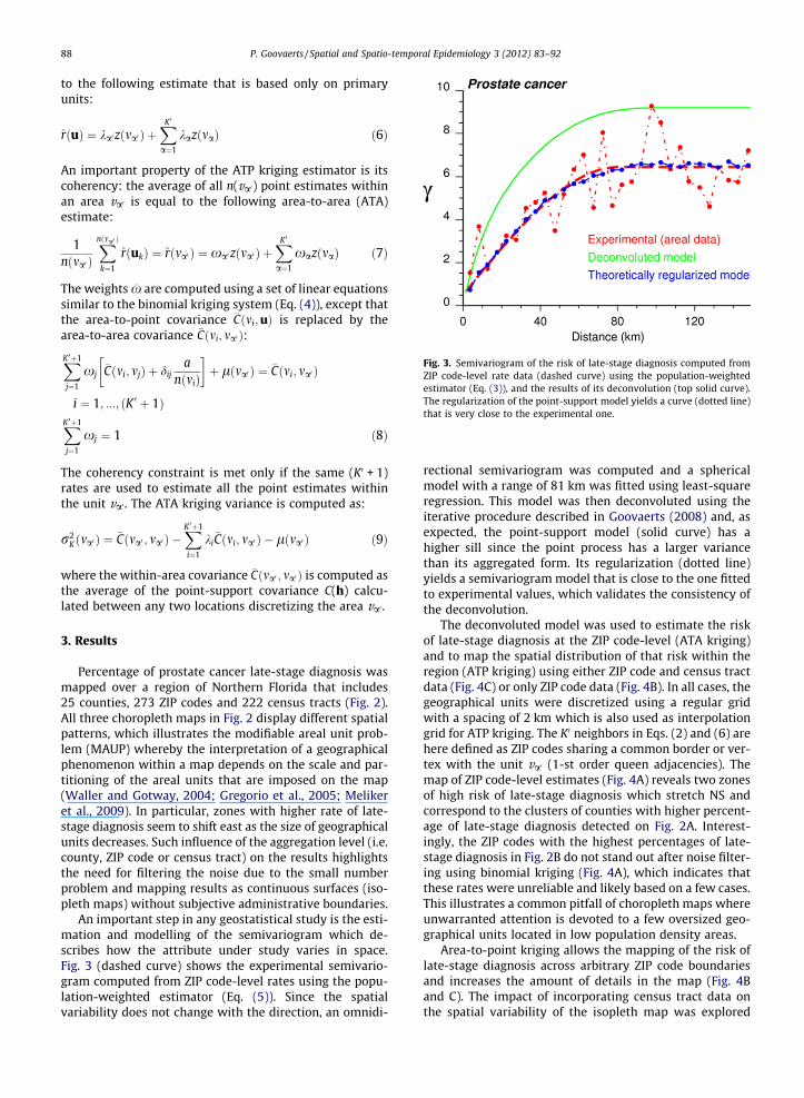
Fig. 3. Semivariogram of the risk of late-stage diagnosis computed fromZIP code-level rate data (dashed curve) using the population-weightedestimator (Eq. (3)), and the results of its deconvolution (top solid curve).The regularization of the point-support model yields a curve (dotted line)that is very close to the experimental one.

88 P. Goovaerts / Spatial and Spatio-temporal Epidemiology 3 (2012) 83–92

to the following estimate that is based only on primaryunits:

rðuÞ ¼ ka0zðma0 Þ þXK 0

a¼1

kazðmaÞ ð6Þ

An important property of the ATP kriging estimator is itscoherency: the average of all n(va0) point estimates withinan area va0 is equal to the following area-to-area (ATA)estimate:

1nðma0 Þ

Xnðma0 Þ

k¼1

rðukÞ ¼ rðma0 Þ ¼ xa0zðma0 Þ þXK 0a¼1

xazðmaÞ ð7Þ

The weights �x are computed using a set of linear equationssimilar to the binomial kriging system (Eq. (4)), except thatthe area-to-point covariance �Cðmi;uÞ is replaced by thearea-to-area covariance �Cðmi; ma0 Þ:

XK 0þ1

j¼1

xj�Cðmi; mjÞ þ dij

anðmiÞ

� �þ lðma0 Þ ¼ �Cðmi; ma0 Þ

i ¼ 1; :::; ðK 0 þ 1ÞXK 0þ1

j¼1

xj ¼ 1 ð8Þ

The coherency constraint is met only if the same (K0 + 1)rates are used to estimate all the point estimates withinthe unit va0. The ATA kriging variance is computed as:

r2Kðma0 Þ ¼ �Cðma0 ; ma0 Þ �

XK 0þ1

i¼1

ki�Cðmi; ma0 Þ � lðma0 Þ ð9Þ

where the within-area covariance �Cðma0 ; ma0 Þ is computed asthe average of the point-support covariance C(h) calcu-lated between any two locations discretizing the area va0.

3. Results

Percentage of prostate cancer late-stage diagnosis wasmapped over a region of Northern Florida that includes25 counties, 273 ZIP codes and 222 census tracts (Fig. 2).All three choropleth maps in Fig. 2 display different spatialpatterns, which illustrates the modifiable areal unit prob-lem (MAUP) whereby the interpretation of a geographicalphenomenon within a map depends on the scale and par-titioning of the areal units that are imposed on the map(Waller and Gotway, 2004; Gregorio et al., 2005; Melikeret al., 2009). In particular, zones with higher rate of late-stage diagnosis seem to shift east as the size of geographicalunits decreases. Such influence of the aggregation level (i.e.county, ZIP code or census tract) on the results highlightsthe need for filtering the noise due to the small numberproblem and mapping results as continuous surfaces (iso-pleth maps) without subjective administrative boundaries.

An important step in any geostatistical study is the esti-mation and modelling of the semivariogram which de-scribes how the attribute under study varies in space.Fig. 3 (dashed curve) shows the experimental semivario-gram computed from ZIP code-level rates using the popu-lation-weighted estimator (Eq. (5)). Since the spatialvariability does not change with the direction, an omnidi-

rectional semivariogram was computed and a sphericalmodel with a range of 81 km was fitted using least-squareregression. This model was then deconvoluted using theiterative procedure described in Goovaerts (2008) and, asexpected, the point-support model (solid curve) has ahigher sill since the point process has a larger variancethan its aggregated form. Its regularization (dotted line)yields a semivariogram model that is close to the one fittedto experimental values, which validates the consistency ofthe deconvolution.

The deconvoluted model was used to estimate the riskof late-stage diagnosis at the ZIP code-level (ATA kriging)and to map the spatial distribution of that risk within theregion (ATP kriging) using either ZIP code and census tractdata (Fig. 4C) or only ZIP code data (Fig. 4B). In all cases, thegeographical units were discretized using a regular gridwith a spacing of 2 km which is also used as interpolationgrid for ATP kriging. The K0 neighbors in Eqs. (2) and (6) arehere defined as ZIP codes sharing a common border or ver-tex with the unit va0 (1-st order queen adjacencies). Themap of ZIP code-level estimates (Fig. 4A) reveals two zonesof high risk of late-stage diagnosis which stretch NS andcorrespond to the clusters of counties with higher percent-age of late-stage diagnosis detected on Fig. 2A. Interest-ingly, the ZIP codes with the highest percentages of late-stage diagnosis in Fig. 2B do not stand out after noise filter-ing using binomial kriging (Fig. 4A), which indicates thatthese rates were unreliable and likely based on a few cases.This illustrates a common pitfall of choropleth maps whereunwarranted attention is devoted to a few oversized geo-graphical units located in low population density areas.

Area-to-point kriging allows the mapping of the risk oflate-stage diagnosis across arbitrary ZIP code boundariesand increases the amount of details in the map (Fig. 4Band C). The impact of incorporating census tract data onthe spatial variability of the isopleth map was explored

Fig. 4. Choropleth maps (ZIP code-level) and isopleth maps of the percentage of late-stage prostate cancer diagnosis estimated by binomial kriging using:ZIP code-level rates (A and B) or ZIP code and census tract-level rates (C). All maps share the same legend that is not documented for confidentiality reasons.

P. Goovaerts / Spatial and Spatio-temporal Epidemiology 3 (2012) 83–92 89

using the semivariogram (Fig. 5A). The cross-over of thetwo curves indicates that this impact varies with the spa-tial scale. Whereas the map based on census tract andZIP code data is globally more variable (i.e. higher sill ofthe semivariogram), the variability at distances shorterthan 15 km is smaller than in the map created using only

ZIP code data. The median extent of the census tracts inthese 25 counties is approximately 17 km assuming asquare shape. Thus, this greater spatial continuity at shortdistances is the direct result of the search strategy: thesame census tract rate is used for interpolating all gridnodes within that tract.

Fig. 5. Impact of incorporating census tract data into ATP kriging: (A) semivariograms of estimates based on ZIP code-level rates (dashed curve) or ZIP codeand census tract-level rates (solid curve), (B) differences between estimates obtained with and without census tract-level rates.

90 P. Goovaerts / Spatial and Spatio-temporal Epidemiology 3 (2012) 83–92

Differences between the two sets of ATP kriging esti-mates are mapped in Fig. 5B, overlaid by the census tractboundaries. Positive differences are balanced by negativedifferences, resulting in a mean difference that is close tozero. Several spatial features in this map bear similaritieswith the patterns displayed by the choropleth maps of ori-ginal rates (Fig. 2B and C). To assess this similarity eachgrid node was assigned the original rates of the censustract and ZIP code in which it lies. The difference betweenthese two rates was then correlated with the difference be-tween ATP kriging estimates at these same nodes. Thestrong rank correlation coefficient (r = 0.618) indicates thatincorporating census tract data influences the most the risk

estimate wherever ZIP code and census tract-level ratesdiffer the most.

In absence of reference values, one cannot state thatone map of estimated risks is more accurate than theother. However, following Zimmerman and Fang (inpress) one should expect the incorporation of additionalinformation to lead to better predictions. In addition,the incorporation of census tract data reduces the krigingvariance by an average of 10% (Fig. 6B and C). As ex-pected, the smallest kriging variances are obtained forZIP code-level estimates (Fig. 6A) since predictions are al-ways more accurate at the area-level compared to thepoint-level.

Fig. 6. Maps of the binomial kriging variance corresponding to the choropleth and isopleth maps of Fig. 4 that were created using: ZIP code-level rates (Aand B) or ZIP code and census tract-level rates (C).

P. Goovaerts / Spatial and Spatio-temporal Epidemiology 3 (2012) 83–92 91

4. Conclusions

A common issue in spatial interpolation is the incorpo-ration of data measured at various scales and over differentspatial supports. This situation is frequently encounteredin health studies where data are typically available over a

wide range of scales, spanning from individual-level to dif-ferent levels of aggregation. In particular this paper focusedon the case where individual-level data are assigned to dif-ferent types of geographical unit based on the success ofthe geocoding and the need to protect patient privacy.The objective was to combine both sources of information

92 P. Goovaerts / Spatial and Spatio-temporal Epidemiology 3 (2012) 83–92

and create maps where disease rates vary continuously inspace, reducing the visual bias associated with the inter-pretation of choropleth maps.

The analysis of prostate cancer data in Florida showedthat incomplete geocoding is a widespread problem, inparticular for cases diagnosed several decades ago and inrural communities. For example, in 1981 one fifth of caseswere not geocoded and this percentage doubled in non-metropolitan counties. The allocation of these cases toZIP codes, combined with the randomization of geocodesconducted by the cancer registry, created two sets of geo-graphical units that can potentially lead to different con-clusions when interpreted separately and without properhandling of the small number problem.

Geostatistics provides a framework to model the spatialcorrelation among health outcomes measured over geo-graphic units of irregular size and population density,and to compute noise-free risk estimates over the sameunits or at much finer scales. A measure of the varianceof prediction errors is also available to identify large andsparsely populated areas where risk estimates are less reli-able. The noise-filtering accomplished by binomial kriginggenerated risk maps with a regional pattern that is closerto the one displayed by the more reliable county-levelrates than by the original ZIP code-level rates. Incorpora-tion of census tract information decreased the kriging var-iance and the within-tract spatial variability whileincreasing the global variability. The impact of using thetwo sets of rates was particularly marked wherever theydiffered the most. The greater accuracy of the risk mapsproduced by the proposed methodology will need to beconfirmed by future simulation studies.

Acknowledgements

This research was funded by grant R44CA132347-02from the National Cancer Institute. The views stated in thispublication are those of the author and do not necessarilyrepresent the official views of the NCI.

References

Cayo MR, Talbot TO. Positional error in automated geocoding ofresidential addresses. Int J Health Geogr 2003;2:10.

Curriero FC, Kulldorff M, Boscoe FP, Klassen AC. Using imputation toprovide location information for nongeocoded addresses. PLoS ONE2010;5(2):e8998. doi:10.1371/journal.pone.0008998.

Goldberg DW, Knoblock CA, Wilson JP. From text to geographiccoordinates: the current state of geocoding. J Urban Reg Inf SystAssoc 2007;19:33–46.

Goovaerts P. Simulation-based assessment of a geostatistical approach forestimation and mapping of the risk of cancer. In: Leuangthong O,Deutsch CV, editors. Geostatistics Banff 2004. Dordrecht: KluwerAcademic Publishers; 2005. p. 787–96.

Goovaerts P. Geostatistical analysis of disease data: accounting for spatialsupport and population density in the isopleth mapping of cancermortality risk using area-to-point Poisson kriging. Int J Health Geogr2006;5:52.

Goovaerts P. Kriging and semivariogram deconvolution in presence ofirregular geographical units. Math Geosci 2008;40:101–28.

Goovaerts P. Combining area-based and individual-level data in thegeostatistical mapping of late-stage cancer incidence. Spat Spatio-tempor Epidemiol 2009;1:61–71.

Goovaerts P. Combining areal and point data in geostatisticalinterpolation: applications to soil science and medical geography.Math Geosci 2010;42:535–54.

Gotway CA, Young LJ. Combining incompatible spatial data. J Am StatAssoc 2002;97:632–48.

Gotway CA, Young LJ. A geostatistical approach to linking geographically-aggregated data from different sources. J Comput Graph Stat2007;16(1):115–35.

Gregorio D, DeChello L, Samociuk H, Kulldorff M. Lumping or splitting:seeking the preferred areal unit for health geography studies. Int JHealth Geogr 2005;4:6.

Hampton KH, Fitch MK, Allshouse WB, Doherty IA, Gesink DC, Leone PA,Serre ML, Miller WC. Mapping health data: improved privacyprotection with donut method geomasking. Am J Epidemiol2010;172(9):1062–9.

Han D, Rogerson PA, Bonner MR, Nie J, Vena JE, Muti P, et al. Assessingspatio-temporal variability of risk surfaces using residential historydata in a case control study of breast cancer. Int J Health Geogr2005;4:9.

Henry KA, Boscoe FP. Estimating the accuracy of geographical imputation.Int J Health Geogr 2008;7:3.

Hibbert JD, Liese AD, Lawson A, Porter DE, Puett RC, Standiford D, Liu L,Dabelea D. Evaluating geographic imputation approaches for zip codelevel data: an application to a study of pediatric diabetes. Int J HealthGeogr 2009;8:54.

Jacquez GM, Rommel R. Local indicators of geocoding accuracy (LIGA):theory and application. Int J Health Geogr 2009;8:60.

Klassen AC, Kulldorff M, Curriero F. Geographical clustering of prostatecancer grade and stage at diagnosis, before and after adjustment forrisk factors. Int J Health Geogr 2005;4:1.

Kravets N, Hadden WC. The accuracy of address coding and the effects ofcoding errors. Health Place 2007;13:293–8.

Krieger N, Waterman PD, Chen JT, Soobader M-J, Subramanian SV, CarsonR. Zip code caveat: bias due to spatiotemporal mismatchesbetween zip codes and US census-defined geographic areas Thepublic health disparities geocoding project. Am J Public Health2002;92:1100–2.

Kyriakidis P. A geostatistical framework for area-to-point spatialinterpolation. Geogr Anal 2004;36:259–89.

Mazumdar S, Rushton G, Smith BJ, Zimmerman DL, Donham KJ.Geocoding accuracy and the recovery of relationships betweenenvironmental exposures and health. Int J Health Geogr 2008;7:13.

Meliker JR, Jacquez GM, Goovaerts P, Copeland G, Yassine M. Spatialcluster analysis of early-stage breast cancer: a method for publichealth practice using cancer registry data? Cancer Causes Control2009;20(7):1061–9.

Rushton G, Armstrong MP, Gittler J, Greene BR, Pavlik CE, West MM,Zimmerman DL. Geocoding in cancer research: a review. Am J PrevMed 2006;30:S16–24.

Strickland MJ, Siffel C, Gardner BR, Berzen AK, Correa A.Quantifying geocode location error using GIS methods. EnvironHealth 2007;6:10.

USDA. Measuring rurality: rural-urban continuum codes: economicresearch service: US Department of Agriculture 2004. http://www.ers.usda.gov/briefing/Rurality/RuralUrbCon/ Accessed July 1,2011.

Waller LA, Gotway CA. Applied spatial statistics for public healthdata. New Jersey: John Wiley and Sons; 2004.

Ward MH, Nuckols JR, Giglierano J, Bonner MR, Wolter C, Airola M, Mix W,Colt JS, Hartge P. Positional accuracy of two methods of geocoding.Epidemiology 2005;16:542–7.

Webster R, Oliver MA, Muir KR, Mann JR. Kriging the local risk of a raredisease from a register of diagnoses. Geogr Anal 1994;26:168–85.

Wieland SC, Cassa CA, Mandl KD, Berger B. Revealing the spatialdistribution of a disease while preserving privacy. Proc Natl AcadSci USA 2008;105:17608–13.

Whitsel EA, Quibrera PM, Smith RL, Catellier DJ, Liao D, Henley AC, HeissG. Accuracy of commercial geocoding: assessment and implications.Epidemiol Perspect Innov 2006;3:8.

Zimmerman DL. Spatial clustering of the failure to geocode and itsimplications for the detection of disease clustering. Stat Med2008a;27:4254–66.

Zimmerman DL. Estimating the intensity of spatial point process fromlocations coarsened by incomplete geocoding. Biometrics2008b;64:262–70.

Zimmerman DL, Fang X. Estimating spatial variation in disease risk fromlocations coarsened by incomplete geocoding. Stat Method in press.doi:10.1016/j.stamet.2011.01.008.

Zimmerman DL, Li J. The effects of local street network characteristics onthe positional accuracy of automated geocoding for geographic healthstudies. Int J Health Geogr 2010;9:10.