Geometry–Aware Finite Element Framework for Multi–Physics Simulations An Algorithmic and Software-Centric Perspective Doctoral Dissertation submitted to the Faculty of Informatics of the Università della Svizzera Italiana in partial fulfillment of the requirements for the degree of Doctor of Philosophy presented by Patrick Zulian under the supervision of Rolf Krause June 2017

Welcome message from author
This document is posted to help you gain knowledge. Please leave a comment to let me know what you think about it! Share it to your friends and learn new things together.
Transcript
Geometry–Aware Finite Element Frameworkfor Multi–Physics Simulations
An Algorithmic and Software-Centric Perspective
Doctoral Dissertation submitted to the
Faculty of Informatics of the Università della Svizzera Italiana
in partial fulfillment of the requirements for the degree of
Doctor of Philosophy
presented by
Patrick Zulian
under the supervision of
Rolf Krause
June 2017


Dissertation Committee
Kai Hormann Università della Svizzera italianaIllia Horenko Università della Svizzera italianaChristian Hesch Universtät SiegenFabian Kuhn University of Freiburg
Dissertation accepted on 30 June 2017
Research Advisor PhD Program Director
Rolf Krause Michael Bronstein
i

I certify that except where due acknowledgement has been given, the workpresented in this thesis is that of the author alone; the work has not been submit-ted previously, in whole or in part, to qualify for any other academic award; andthe content of the thesis is the result of work which has been carried out sincethe official commencement date of the approved research program.
Patrick ZulianLugano, 30 June 2017
ii

Dedicated to my wife Giorgiana, family, and friends.
iii

iv
“In mathematics you don’tunderstand things, you just getused to them”
John von Neumann
v

vi
Abstract
In finite element simulations, the handling of geometrical objects and their dis-crete representation is a critical aspect in both serial and parallel scientific soft-ware environments. The development of codes targeting such envinronments issubject to great development effort and man-hours invested. In this thesis weapproach these issues from three fronts.
First, stable and efficient techniques for the transfer of discrete fields betweennon matching volume or surface meshes are an essential ingredient for the dis-cretization and numerical solution of coupled multi-physics and multi-scale prob-lems. In particular L2-projections allow for the transfer of discrete fields betweenunstructured meshes, both in the volume and on the surface. We present an algo-rithm for parallelizing the assembly of the L2-transfer operator for unstructuredmeshes which are arbitrarily distributed among different processes. The algo-rithm requires no a priori information on the geometrical relationship betweenthe different meshes.
Second, the geometric representation is often a limiting factor which imposesa trade-off between how accurately the shape is described, and what methodscan be employed for solving a system of differential equations. Parametric finite-elements and bijective mappings between polygons or polyhedra allow us to flex-ibly construct finite element discretizations with arbitrary resolutions withoutsacrificing the accuracy of the shape description. Such flexibility allows employ-ing state-of-the-art techniques, such as geometric multigrid methods, on mesheswith almost any shape.
Last, the way numerical techniques are represented in software libraries andapproached from a development perspective affect both usability and maintain-ability of such libraries. Completely separating the intent of high-level routinesfrom the actual implementation and technologies allows for portable and main-tainable performance. We provide an overview on current trends in the develop-ment of scientific software and showcase our open-source library UTOPIA.
vii

viii

Acknowledgements
The author would like to thank the people and institutions that have been in-tegral to the realization of this work. Prof. Dr. Rolf Krause for his advise andsupport during my PhD studies. Teseo Schneider for his help and collaborationin realizing the project which embodies Chapter 4, and for constant exchangeof ideas and discussions. Dr. Lea Conen for her contributions for a help in thewriting of Section 2.2 and Section 3.3. Alena Kopanicáková for her work on theUTOPIA solver modules and the integration of UTOPIA with the MOOSE library,and her contribution with the phase-phield example in Chapter 5. Dr. MariaGiuseppina Chiara Nestola for here help in integrating the parallel transfer algo-rithm of MOONOLITH with LIBMESH and MOOSE. Prof. Dr. Panayot Vassileskifor the mentorship during my work at the Lawrence Livermore National Labora-tory which led to the integration of MOONOLITH within their in-house softwareMFEM.
This work and the development of the related software libraries is partlysupported by the Swiss National Science Foundation (http://www.snf.ch) un-der projects “Geometry-Aware FEM in Computational Mechanics” (No.:156178),“ExaSolvers – Extreme scale solvers for coupled systems” (No.:145271), “Paral-lel multilevel solvers for coupled interface problems” (No.:146167), “Large-scalesimulation of pneumatic and hydraulic fracture with a phase-field approach”(No.:154090), and by the SCCER-FURIES program (http://sccer-furies.epfl.ch).
ix

x
Contents
Contents xi
1 Introduction 11.1 Thesis structure . . . . . . . . . . . . . . . . . . . . . . . . . . . . . . . 4
2 Geometry based techniques and abstraction tools in scientific soft-ware 52.1 Weak transfer between discrete spaces . . . . . . . . . . . . . . . . . 52.2 Formulation . . . . . . . . . . . . . . . . . . . . . . . . . . . . . . . . . 8
2.2.1 Mortar projection . . . . . . . . . . . . . . . . . . . . . . . . . 92.2.2 L2-projection and pseudo-L2-projection . . . . . . . . . . . . 122.2.3 Relation to the application scenarios . . . . . . . . . . . . . . 14
2.3 Procedure for the assembly of the coupling operators . . . . . . . . 162.3.1 Assembly procedure for two-body contact problems . . . . 182.3.2 Non–affine elements and quadrature points . . . . . . . . . 22
2.4 Space partitioning and ordering . . . . . . . . . . . . . . . . . . . . . 232.4.1 Space-subdivision strategies and acceleration data–structures 232.4.2 Bounding volumes . . . . . . . . . . . . . . . . . . . . . . . . . 242.4.3 Spatial hashing . . . . . . . . . . . . . . . . . . . . . . . . . . . 242.4.4 Space-partitioning trees and bounding volume hierarchies 252.4.5 Space-filling curves and linear octree/quadtree represen-
tations . . . . . . . . . . . . . . . . . . . . . . . . . . . . . . . . 262.4.6 Advancing front algorithms . . . . . . . . . . . . . . . . . . . 27
2.5 Parametrizations and finite element discretizations . . . . . . . . . 282.5.1 Composite mean value mappings . . . . . . . . . . . . . . . . 292.5.2 Efficient computation of the Jacobian matrix of the com-
posite mean-value mapping . . . . . . . . . . . . . . . . . . . 312.6 Software libraries and tools for scientific computing . . . . . . . . . 332.7 Chapter conclusion . . . . . . . . . . . . . . . . . . . . . . . . . . . . . 34
xi

xii Contents
3 Parallel transfer of discrete fields for arbitrarily distributed unstruc-tured finite element meshes 353.1 Parallel pipeline . . . . . . . . . . . . . . . . . . . . . . . . . . . . . . . 363.2 Parallel intersection/proximity detection . . . . . . . . . . . . . . . . 37
3.2.1 A parallel tree-search algorithm . . . . . . . . . . . . . . . . . 373.2.2 Extended data-structures for pruning . . . . . . . . . . . . . 443.2.3 Multiple meshes and multi-domain meshes per process . . 44
3.3 Application based assembly . . . . . . . . . . . . . . . . . . . . . . . . 453.3.1 Element-wise block operator representation . . . . . . . . . 463.3.2 Handling of assembled quantities in contact problem . . . 47
3.4 Implementation . . . . . . . . . . . . . . . . . . . . . . . . . . . . . . . 473.5 Chapter conclusion . . . . . . . . . . . . . . . . . . . . . . . . . . . . . 48
4 Parametric finite elements with bijective mappings 514.1 Formulation . . . . . . . . . . . . . . . . . . . . . . . . . . . . . . . . . 524.2 Shape and volume parameterization . . . . . . . . . . . . . . . . . . 56
4.2.1 Constructing the parameterization domain . . . . . . . . . . 574.2.2 Pre–computation of the composite mean value mapping . 58
4.3 Piecewise mapping approximations . . . . . . . . . . . . . . . . . . . 594.3.1 Polynomial elements . . . . . . . . . . . . . . . . . . . . . . . 594.3.2 Polygonal elements . . . . . . . . . . . . . . . . . . . . . . . . 604.3.3 Piecewise affine elements . . . . . . . . . . . . . . . . . . . . 61
4.4 A multigrid method for arbitrarily shaped 2D meshes using para-metric finite elements . . . . . . . . . . . . . . . . . . . . . . . . . . . 64
4.5 Chapter conclusion . . . . . . . . . . . . . . . . . . . . . . . . . . . . . 65
5 Utopia: a C++ embedded domain specific language for scientific com-puting 695.1 Architecture . . . . . . . . . . . . . . . . . . . . . . . . . . . . . . . . . 70
5.1.1 Embedded domain specific language . . . . . . . . . . . . . . 715.1.2 Expression tree . . . . . . . . . . . . . . . . . . . . . . . . . . . 715.1.3 Evaluator . . . . . . . . . . . . . . . . . . . . . . . . . . . . . . 755.1.4 API and memory access transparency . . . . . . . . . . . . . 78
5.2 Extensions . . . . . . . . . . . . . . . . . . . . . . . . . . . . . . . . . . 795.2.1 Solvers as eDSL primitives . . . . . . . . . . . . . . . . . . . . 805.2.2 Finite element assembly . . . . . . . . . . . . . . . . . . . . . 815.2.3 Visualization and debugging . . . . . . . . . . . . . . . . . . . 82
5.3 Applications . . . . . . . . . . . . . . . . . . . . . . . . . . . . . . . . . 835.4 Chapter conclusion . . . . . . . . . . . . . . . . . . . . . . . . . . . . . 91
xiii Contents
6 Numerical experiments 936.1 Parallel transfer . . . . . . . . . . . . . . . . . . . . . . . . . . . . . . . 93
6.1.1 Hardware . . . . . . . . . . . . . . . . . . . . . . . . . . . . . . 956.1.2 Weak-scaling experiments . . . . . . . . . . . . . . . . . . . . 956.1.3 Strong-scaling experiments . . . . . . . . . . . . . . . . . . . 956.1.4 Particular scenarios . . . . . . . . . . . . . . . . . . . . . . . . 976.1.5 Scaling and output-sensitivity . . . . . . . . . . . . . . . . . . 100
6.2 Parametric finite elements with bijective mappings . . . . . . . . . 1006.2.1 Convergence . . . . . . . . . . . . . . . . . . . . . . . . . . . . 1016.2.2 Comparison . . . . . . . . . . . . . . . . . . . . . . . . . . . . . 1026.2.3 Conditioning . . . . . . . . . . . . . . . . . . . . . . . . . . . . 1056.2.4 Convergence of the multigrid method with parametric fi-
nite elements . . . . . . . . . . . . . . . . . . . . . . . . . . . . 1066.3 Chapter conclusion . . . . . . . . . . . . . . . . . . . . . . . . . . . . . 111
7 Conclusion 113
Bibliography 115

xiv Contents
Chapter 1
Introduction
The finite element method [17; 44; 108] is a well established and known tech-nique for the solution of partial differential equations. A great effort is investedin the development of software libraries implementing finite element assemblyprocedures and related solution algorithms. In fact, the development of suchsoftware libraries has several challenges.
The first challenge is dealing with complex mathematical models and simulat-ing multiple physical phenomena simultaneously. This typically involves solvingcoupled systems of differential equations which might even require different dis-cretizations (e.g., molecular dynamics). The complexity of solving this problemsrises when we introduce complex geometries having non-trivial interactions witheach other, for instance contact between solids.
The second challenge is taking advantage of the concurrency within com-putational problems and taking advantage of the hardware resources availablein modern super-computers. A significant amount of effort is invested in thedevelopment of parallel codes, and in new numerical methods/algorithms foroptimally exploiting the available parallelism. As a consequence, scientific soft-ware becomes ever more complex and hard to reuse, re-purpose, maintain andextend.
The third challenge is the handling of geometric descriptions and the accu-racy of their discrete representations. Embodying accurate representations withoptimal and completely automatic black-box usage of state-of-the-art solvers is anon-trivial task.
The last challenge is modularity and usability of scientific software libraries.A reusable implementation of very complex algorithms is an important factor.The costs and effort of developing even only one such functionality might besignificant. Hence, proper use of software design patterns and abstractions is
1
2
relevant for users at any level of involvement in the development of scientificcodes. For instance, for solving a PDE with standard methods, users need only aminimal set of abstractions without having to deal with low level implementationdetails. Users that are researching new methods may however require access tospecialized lower level abstractions. This aspects are strictly related to the issueof usability. It is often the case that scientific software imposes high barriers toentry for newcomers or inexperienced users. The presence of such high barriersis translated to poor productivity for new library adopters. For circumventingthese challenges, a current trend in scientific software development is to strivefor higher level abstractions.
This thesis is an attempt to contributing in dealing with the aforementionedchallenges by covering three topics.
Parallel transfer of discrete fields for arbitrarily distributed unstructured finiteelement meshes
We present and investigate a new and completely parallel approach for the trans-fer of discrete fields between non-matching volume or surface meshes, arbitrarilydistributed among different processors. No a priori information on the relationbetween the different meshes is required. Our inherently parallel approach isgeneral in the sense that it can deal with both classical interpolation and vari-ational transfer operators, e.g., the L2-projection and the pseudo-L2-projection.It includes a parallel search strategy, output dependent load balancing, and thecomputation of element intersections, as well as the parallel assembling of thealgebraic representation of the respective transfer operator. We describe our al-gorithmic framework and its implementation in the library MOONOLITH. Fur-thermore, we investigate the efficiency and parallel scalability of our new ap-proach using different examples in 3D. This includes the computation of a vol-ume transfer operator between 2 meshes with 2 billion elements in total andthe computation of a surface transfer operator between 14 different meshes with5.9 billion elements in total. The experiments have been performed with up to12 288 cores.
Parametric finite elements with bijective mappings
We present a novel approach which combines parametric finite elements withsmooth bijective mappings which allows to decouple the choice of approxima-tion spaces from the geometric shape. Our approach allows to represent arbi-trarily complex geometries on coarse meshes with curved edges, regardless of
3
the domain boundary complexity. The main idea is to use a bijective mappingfor automatically warping the volume of a simple parameterization domain tothe complex computational domain, thus creating a curved mesh of the latter.The numerical examples confirm that our method has lower approximation er-ror than the standard finite element method, because we are able to solve theproblem directly on the exact shape of domain without having to approximateit. In other words our method allows solving the model problem on the exactgeometry with the freedom of choosing the discretization independently. Thisfreedom enables to employ state-of-the-art solution strategies such as the multi-grid method. Our discretization allows to automatically generate the meshesof a multigrid hierarchy just by refining a coarse mesh in the parameterizationdomain. This contribution is the result of a joint project and work with TeseoSchneider and Kai Hormann.
Utopia: a C++ embedded domain specific language for scientific computing
We present UTOPIA, a C++ embedded domain specific language designed for par-allel non-linear solution strategies and finite element analysis. The rise of newcomputing hardware and the continuous development of numerical methodsand programming technologies/languages/paradigms are drivers for changes inscientific-computing software libraries. However, such changes affect both thecomputing libraries and their dependencies, inducing unwanted modifications tohigh-level code. For avoiding these unwanted modifications, state-of-the-art soft-ware mainly relies on high-level programming interfaces or scripting languages.UTOPIA combines advantages of high-level programming interfaces with the ad-vantages of scripting languages. On the one hand, it allows using high-levelabstractions while providing access to the native low-level data-structures. Onthe other hand, it facilitates expressing complex numerical procedures by meansof few lines of code. This is achieved by separating the model from the compu-tation, thus allowing to keep the implementation details hidden from the codeof applications such as non-linear solution algorithms and finite element assem-bly. We achieve this separation by using C++ meta-programming and particu-lar evaluation strategies which allow mapping an abstract representation of thecomputation to the actual code computing the result. The linear algebra andfinite element assembly codes snippets provides examples of the expressivenessof UTOPIA.
4 1.1 Thesis structure
1.1 Thesis structure
In Chapter 2 we introduce the related work which includes mortar projectionmethods, parametric finite elements, and state of the art scientific software li-braries. In Chapter 3 we described in detail a novel parallel algorithm for thetransfer of discrete fields between arbitrarily distributed unstructured finite ele-ment meshes. In Chapter 4 we introduce a novel discretization based on para-metric finite elements. In Chapter 5 we showcase the UTOPIA domain specificlanguage and software library. In Chapter 6 we illustrate the performance studiesof our parallel transfer algorithm and numerical experiments of our parametricfinite element discretization. In Chapter 7 we briefly discuss general aspects ofthis thesis and its contributions.

Chapter 2
Geometry based techniques andabstraction tools in scientificsoftware
In this chapter we introduce the related work. We describe the existing mathe-matical methods for exchanging information between finite element spaces (Sec-tion 2.1 and Section 2.2) and we provide a detailed introduction of the proce-dures (Section 2.3) and the geometric tools (Section 2.4) necessary to implementsuch methods. We briefly introduce existing methods for working with differentgeometric representations, and our method of choice for creating volume pa-rameterizations (Section 2.5). We provide an overview of available open-sourcefinite element software libraries from a software design/development perspec-tive (Section 2.6).
2.1 Weak transfer between discrete spaces
The ever increasing computational power of modern super-computers allows,nowadays, for the numerical simulation of complex and coupled large scale prob-lems, as arising from contact or fracture mechanics, fluid-structure interaction,computational geo-science, computational medicine, or, more general, multi-physics and multi-scale problems. Common to all these coupled and complexproblems is the need for the transfer of data or information between the differ-ent models, meshes, or approximation spaces. The transfer of discrete fields asstresses, pressure, displacements, or velocities might be required along surfaces,e.g., in the case of contact mechanics or fluid structure interaction, or withinvolumes, e.g., in the case of transient simulations or multi-scale simulations. Ad-
5

6 2.1 Weak transfer between discrete spaces
ditionally, the transfer of discrete fields might also play an important role on thelevel of the discretization, e.g., within non-conforming domain decomposition ormortar methods for the transfer along surfaces, or on the level of the solutionmethod, e.g., within multigrid or multi-level methods for the transfer betweendifferent volume meshes.
Clearly, the way transfer operators are constructed affects the quality of theused methods in terms of convergence, accuracy, and efficiency [53]. Thus, be-sides classical interpolation, more recently transfer operators based on varia-tional approaches, such as (pseudo-)L2-projections, have been developed. Here,in particular the mortar method [13] has to be mentioned, which has given riseto a huge number of new algorithmic developments during the last decades.
Despite these advances, deploying these approaches in a parallel high per-formance computing environment, the actual computation of such a volume orsurface transfer operator turns out to be far from trivial. Different unstructuredmeshes might be arbitrarily distributed in a possibly unrelated manner, lead-ing to many possible data distribution scenarios, which have to be handled in atransparent and efficient way. Additionally, the issues of scalability, usability andflexibility arise.
In our discussion we consider the general parallel case where we do not haveany prior assumption on the spatial and memory location of the geometric ob-jects. We focus our attention on the transfer of information of functional quanti-ties from one mesh — or approximation space connected to a mesh — to another.Note that the actual choice of the approximation space may arise from finite el-ements, finite volumes or spectral methods. Here, we mainly consider the finiteelement method, as it is well known for dealing efficiently with complex unstruc-tured geometries. For a more specific scenario we refer to [79], where the au-thors describe a technique for the parallel coupling between finite elements andmolecular dynamics in a multi-scale method using a variational scale transfer.
In a parallel environment, the main challenges are identifying and handlingrelationships between geometric objects of interest based on spatial informa-tion, the used discretization and the application requirements. Given that a highdegree of flexibility and generality is sought, the technical ingredients neces-sary for the realization of such strategies originates from different disciplinessuch as applied mathematics, geometric algorithms, software design, and high-performance computing.
There is a large number of different applications that might profit from ascalable parallel information transfer as presented herein:
• Complex parallel multi-physics problems. The handling of multiple types of
7 2.1 Weak transfer between discrete spaces
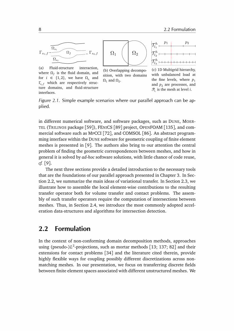
non-conformities in complex simulation scenarios with multiple geometriesis usually done ad-hoc. A completely automated online strategy might al-low more complex transient scenarios [63]. A common scenario, illustratedin the diagram in Figure 2.1(a), would be fluid-structure interaction andstructure-structure interaction, where the fluid mesh is unstructured [64].See [30; 94] for a comprehensive review of coupling methods in the con-text of fluid-structure interaction.
• Coupling of distributed meshes in non-conforming overlapping domain de-composition methods such as additive Schwarz [109], as illustrated by thediagram in Figure 2.1(b).
• Handling of non-penetration conditions in parallel contact problem simula-tions [138]. The contact surfaces between bodies are not always knowna priori and they are in general geometrically non-conforming.
• Parallel remeshing in transient simulations, such as large deformations incomputational mechanics. Local remeshing without having to ensure con-formity at the subdomain interface allows for complete parallelization.
• Handling of distributed multigrid hierarchies. The coarse meshes can be se-lected without the restriction of requiring the same shape of the geometryor nested elements. The freedom to handle the various levels of refinementin a completely arbitrary way makes it possible to easily provide better bal-anced computations. For instance, as shown in Figure 2.1(c), cases wherethe hierarchy is generated by refining a coarse mesh into finer levels with-out balancing the computational load might lead to bad scaling. The ap-proach we present in Chapter 3 allows constructing prolongation/restric-tion operators without requiring the additional programming of complexparallel code.
• Multi-scale simulations, e.g., the coupling of molecular dynamics and finiteelements as in [78; 139].
Additionally, numerical non-linear solution method can profit from non-conformingdomain decomposition strategies such as in [54]. Extensive coverage of relatedmatters, such as Galerkin projection methods, and intersection reporting can befound in [45; 46].
Let us comment on already existing approaches and their respective imple-mentations. The question of variational information transfer has been addressed
8 2.2 Formulation
⌦f
⌦s1
⌦s2
�s2,f�s1,f⌦1 ⌦2
p1 p2T hl1
T hl2
T hl3
(a) Fluid-structure interaction,where ⌦ f is the fluid domain, andfor i 2 {1, 2}, we have ⌦si
and�si , f which are respectively struc-ture domains, and fluid-structureinterfaces.
(b) Overlapping decompo-sition, with two domains⌦1 and ⌦2.
(c) 1D Multigrid hierarchy,with unbalanced load atthe fine levels, where p1and p2 are processes, andTli
is the mesh at level i.
Figure 2.1. Simple example scenarios where our parallel approach can be ap-plied.
in different numerical software, and software packages, such as DUNE, MOER-TEL (TRILINOS package [59]), FENICS [89] project, OPENFOAM [135], and com-mercial software such as MPCCI [72], and COMSOL [86]. An abstract program-ming interface within the DUNE software for geometric coupling of finite elementmeshes is presented in [9]. The authors also bring to our attention the centralproblem of finding the geometric correspondences between meshes, and how ingeneral it is solved by ad-hoc software solutions, with little chance of code reuse,cf. [9].
The next three sections provide a detailed introduction to the necessary toolsthat are the foundations of our parallel approach presented in Chapter 3. In Sec-tion 2.2, we summarize the main ideas of variational transfer. In Section 2.3, weillustrate how to assemble the local element-wise contributions to the resultingtransfer operator both for volume transfer and contact problems. The assem-bly of such transfer operators require the computation of intersections betweenmeshes. Thus, in Section 2.4, we introduce the most commonly adopted accel-eration data-structures and algorithms for intersection detection.
2.2 Formulation
In the context of non-conforming domain decomposition methods, approachesusing (pseudo-)L2-projections, such as mortar methods [13; 137; 82] and theirextensions for contact problems [34] and the literature cited therein, providehighly flexible ways for coupling possibly different discretizations across non-matching meshes. In our presentation, we focus on transferring discrete fieldsbetween finite element spaces associated with different unstructured meshes. We

9 2.2 Formulation
(a) Source mesh. (b) Source mesh cut. (c) Target mesh.
Figure 2.2. Example of volume information transfer between different meshes.A given finite-element function on a cube (a) and (b), is transferred to a morecomplex geometry, i.e., a hand (c).
note, however, that the techniques described herein are rather general and canbe also applied to other types of discretizations, such as finite volume or spectralmethods. Similar efforts for similar purpose include the Arlequin method [12].
2.2.1 Mortar projection
We start our discussion with a short introduction of the mortar projection, whichwill be used in our numerical experiments. For a comparison of different pro-jection operators and their quantitative properties we refer the interested readerto [36].
For a (bounded) domain ⌦ ⇢ Rd with Lipschitz boundary, let L2(⌦) be, asusual, the Hilbert space of square integrable functions on ⌦ with inner product(v, w)L2(⌦) =
R⌦
vw dx and norm k ·kL2(⌦) = (·, ·)1/2L2(⌦). Let ⌦m,⌦s ⇢ Rd be bounded(Lipschitz) domains. Let the intersection I = ⌦m \ ⌦s of the two domains andthe spaces V = L2(⌦m), W = L2(⌦s) be given.
We assume that ⌦m and ⌦s can be approximated, respectively, by the discretedomains ⌦h
m and ⌦hs . Let the mesh Tk =
�Ek ✓ ⌦h
k |S
Ek = ⌦hk
, with k 2 {m, s},
be a finite set, where its elements Ek form a partition, hence if E1k , E2
k ✓ ⌦hk and
E1k 6= E2
k then E1k \ E2
k = ;. For simplicity we consider Tk, k 2 {m, s} to beconforming, though our approach is also applicable to the non-conforming case.
We denote the associated finite element spaces by Vh = Vh(Tm) and Wh =Wh(Ts). For non-matching meshes Tm and Ts, also the approximation spaces Vh
and Wh differ. We define the intersection of the two discrete domains as Ih =⌦h
m \⌦hs , and assume that Ih 6= ;. Furthermore, with Nm and Ns we denote the
respective set of nodes of the meshes.
10 2.2 Formulation
The case ⌦hs ✓ ⌦h
m
For simplicity, we now assume ⌦hs ✓ ⌦h
m. For this case, the projection has beenshown to be stable [137]. We consider the case ⌦h
s 6✓ ⌦hm in Section 2.2.1. For the
definition of the projection operator, we also need to define a suitable discretespace of Lagrange multipliers Mh. We here set Mh = Mh(Ts), i.e., Mh is a discretespace based on the same mesh as Wh. The association of Mh with either Tm orTs is arbitrary but fixed. Following the naming convention in the literature onmortar methods, the space associated with Mh, that is Wh, is often referred toas slave, or non-mortar, and the other one, that is Vh, as master, or mortar. Themortar projection maps a function from the mortar space, i.e., Vh in our case, tothe non-mortar space, i.e., Wh.
Now we proceed to the definition of the projection operator P : Vh!Wh. Fora function vh 2 Vh we want to find wh = P(vh) 2Wh, such that
(P(vh),µh)L2(Ih) = (vh,µh)L2(Ih) 8µh 2 Mh. (2.1)
Reformulating Equation (2.1), cf. [13], we get the “weak equality” conditionZ
Ih
(vh � P(vh))µh dx=Z
Ih
(vh � wh)µh dx= 0 8µh 2 Mh. (2.2)
Let {�i}i2Jvbe a basis of Vh, {✓ j} j2Jw
of Wh, and { k}k2Jµ of Mh, where Jv, Jw, andJµ ⇢ N are index sets. Now writing the functions vh 2 Vh and wh 2 Wh in termsof the respective bases, we get vh =
Pi2JV vi�i, and wh =
Pj2JW wj✓ j, where
{vi}i2Jvand
�wj
j2Jw
are real coefficients. This allows us to write the point-wisecontributions to Equation (2.2) as
X
i2Jv
vi
Z
Ih
�i k dx=X
j2Jw
w j
Z
Ih
✓ j k dx for k 2 Jµ. (2.3)
We rewrite Equation (2.3) as a matrix equation using the matrices B and D withrespective entries bk,i =
RIh�i k dx, and dk, j =
RIh✓ j k dx, i 2 Jv, j 2 Jw, k 2 Jµ:
Bv= Dw. (2.4)
Here, v and w are vectors of coefficients with respective entries vi and wj. Fromnow on assume that the matrix D is square, that is |Jw| =
��Jµ�� and thus Wh and
Mh have the same dimension. Additionally, we assume that D is invertible andthus we define the algebraic representation of the discrete (mortar) projectionoperator as T= D�1B and rewrite Equation (2.4) as
w= D�1Bv= Tv.
11 2.2 Formulation
Depending on the choice of Mh, we obtain different transfer operators T. Forinstance, using what is known as the dual basis for Mh, the matrix D becomesdiagonal (or possibly block-diagonal for systems of equations). For details onthis choice of Mh see Section 2.2.2.
The case ⌦hs 6✓ ⌦h
m
For this case we do not provide stability guarantee on the projections. Due to⌦h
s 6✓ ⌦hm, we need to consider the extension to ⌦h
m [⌦hs of the functions vh 2 Vh
by means of an extension operator. For Lipschitz domains, the existence of acontinuous extension operator can be guaranteed [136, Theorem 5.3, Page 95].In practice, different extension operators could be chosen, for example extensionby zero, harmonic extension, or constant in the direction of the outer surfacenormal [75]. Eventually, this choice depends on the application.
Let J Iv = {i 2 Jv| supp (�i)\ Ih 6= ;}, J I
w =�
j 2 Jw| supp�✓ j
�\ Ih 6= ; , and
J Iµ =
�k 2 Jµ| supp ( k)\ Ih 6= ;
be the index sets of the basis functions of Vh,
Wh, and Mh, respectively, with support in the intersection region Ih. By restrictingthe spaces Vh and Wh to Ih, we have the following new spaces
Xh = Vh|Ih= span
i2J Iv
��i ·�Ih
, Yh = Wh|Ih
= spanj2J I
w
�✓ j ·�Ih
,
where �Ihis the characteristic function on Ih defined as
�Ih(x) =
®1 if x 2 Ih,
0 else.
In order to adapt the definition of the projection operator to this case, we alsodefine a modified version Mh = spank2J I
µ
� k
of the multiplier space Mh =
spank2Jµ { k}, where
k =
® k|Ih
: if supp ( k) ✓ Ih
�k : if supp ( k) 6✓ Ih8k 2 J I
µ. (2.5)
Here �k is a function defined on the intersection Ih. The functions �k are notnecessarily the restrictions k|Ih
of k to the intersection region Ih, but theirdefinition depends on the choice of the multiplier space Mh. As Mh so far is ageneric space, we here do not define �k. For an example construction in the caseof the pseudo-L2-projection see Section 2.2.2.
12 2.2 Formulation
We can now adapt the definition of the projection operator P to the case⌦h
s 6✓ ⌦hm. For a function vh 2 Xh we hence want to find wh = P(vh) 2 Yh, such
that(P(vh), µh)L2(Ih) = (vh, µh)L2(Ih) 8µh 2 Mh.
We can then derive the discrete projection operator T as in Section 2.2.1 underthe assumption that Wh and Mh have the same dimension. As a final remark,we note that with this definition of the spaces Xh and Yh, the projected functionwh = P (vh) 2 Yh is by definition zero in ⌦h
s \ Ih. Other extensions to ⌦hs \ Ih are
possible.
2.2.2 L2-projection and pseudo-L2-projection
In the preceding definition of the projection operator T, we are still free to choosethe multiplier space Mh. Different choices of Mh will lead to different projec-tion operators. Setting for example Mh = Wh, T is the discrete representationof the L2-projection. In this case, even though the mass matrix D is typicallywell-conditioned, the evaluation of T= D�1B might become computationally ex-pensive, or not convenient. It might be expensive because the inverse of D isdense. Hence, instead of storing T, keeping D and B as separate matrices mightbe a better solution. However, this implies that each time we apply the transferoperator we solve a linear system. This is less convenient than storing only onematrix that can be applied directly.
We therefore consider mainly the case of choosing dual basis functions as abasis for Mh, as presented originally in [137]. In this case, the multiplier spaceMh is spanned by a set of functions which are biorthogonal to the basis functionsof Wh with respect to the L2-inner product. This makes the matrix D diagonal,and computing its inverse cheap. In practice the matrix D is a lumped mass-matrix.
Since the vector space Wh is finite-dimensional, the dual basis exists, and thedimension of the dual space is the same as the one of the original space. Ingeneral, the dual basis functions k, k 2 Jµ = Jw, might have global support.Under certain assumptions on the space Wh, they can however be constructedelementwise in such a way that
supp ( k) ✓ supp (✓k) =:!k 8k 2 Jw (2.6)
holds, i.e., that their support is restricted to one finite element patch !k. This isfor example possible assuming that Wh is the standard degree one finite elementspace and
�✓ j
j2Jw
is the standard basis [32].
13 2.2 Formulation
In the case ⌦hs ✓ ⌦h
m, we choose the multiplier space as the discontinuous testspace
Mh = span{ k : Ih! R| k 2 Jw, supp ( k) ✓!k} 6✓ C0(Ih), (2.7)
where the functions k satisfy the following biorthogonality condition:
( k,✓ j)L2(Ih) = � j,k(✓ j,1)L2(Ih) 8 j, k 2 Jw. (2.8)
As described in [32; 47], a basis { k}k2Jwfulfilling (2.7) and (2.8) can be
constructed in a straightforward way, using only computations on single ele-ments. Let E 2 Ts be one element in the mesh of the finite element space Wh. LetME =
�mpq
�be an element mass matrix, and DE =
�dpq
�be an element diagonal
matrix defined by
mpq =�✓p,✓q
�L2(E) , dpq = �pq
�✓p,1
�L2(E) 8p, q 2 Ns \ E,
respectively, whereNs are the nodes of Ts, and E is the closure of the element E ofmesh Ts. As ME is symmetric positive definite and thus invertible, for p 2 Ns \ Ewe can define functions p,E by
p,E(x) :=
®Pr2Ns\E
�DE M�1
E
�pr ✓r(x) if x 2 E,
0 else.(2.9)
Then we can define the dual basis fulfilling (2.7) and (2.8) by
p =X
E2Ts: p2E
p,E 8p 2 Ns. (2.10)
We furthermore note that in the case of affine elements, due to the scaling with(✓ j,1)L2(Ih) on the right-hand side of Equation (2.8), the coefficients in Equa-tion (2.9) do not depend on the element E or the node p [32]. Thus it is sufficientto compute them only once on the reference element. Furthermore, in this case,the dual basis function k is continuous on the patch!k, that is k|!k
2 C0(!k).In the case where⌦h
s 6✓ ⌦hm, and Ih = ⌦h
s\⌦hm 6= ;, we provide an example for a
modified multiplier space. We would like to stress that our framework is generalin the sense that multiplier and approximation spaces can be freely prescribedby the user. In our example, let the discontinuous test space be
Mh = span{ k : Ih! R| k 2 J Iw, supp
� k
� ✓ !k} 6✓ C0(Ih), (2.11)
where !k is the support of the k-th basis function of Yh, and the functions k
with support in !k satisfy the following biorthogonality condition:
( k,✓ j)L2(Ih) = �p,q(✓ j,1)L2(Ih) 8 j, k 2 J Iw. (2.12)
14 2.2 Formulation
Hence� k
is the dual basis with respect to the basis
�✓k ·�Ih
of Yh.
As in the previous case, we can construct the dual basis elementwise byslightly modifying the above procedure. More precisely, we restrict all indicesto the smaller index set J I
w, and replace ✓k by ✓k · �Ihfor all k. This implicitly
defines the functions �k in Equation (2.5).In this case, even for affine elements, for an element E that is not completely
contained in the intersection, i.e., E 6✓ Ih and E \ Ih 6= ;, the coefficients in themodified Equation (2.9) do depend on the element and on the node. Thus thelocal matrices DE and ME need to be computed and ME needs to be inverted onevery such element separately. Moreover, this implies that the function k is ingeneral not continuous on its support. If E \ Ih is small, the jump in the func-tion k might become large, leading to instabilities in the method. This problemcan be handled by considering intersections with really small volume as empty.Numerically speaking, we consider the intersections supp (.)\ Ih to be empty, iftheir volumes are smaller than a small numerical constant. We emphasize thatthis is an ad-hoc solution, which has turned out to work well in practice, whichdoes no affect the overall approach.
The pseudo-L2-projection is a projection, and it also guarantees an efficientevaluation of the transfer operator T. In fact, using dual basis functions, T canbe evaluated easily, as D becomes diagonal (or block-diagonal in the case of sys-tems). Thus, the usage of dual basis functions corresponds to replacing the stan-dard L2-projection by a pseudo-L2-projection, which allows for a more efficientassembly and application of T.
As investigated numerically in the study performed in [36], the pseudo-L2-projection is close to the L2-projection in terms of the operator norm. The pseudo-L2-projection is also proven to be H1-stable and has the L2-approximation prop-erty for all shape-regular families of meshes (see [137; 32] for more details). Allof the numerical experiments presented in this thesis employ this operator.
2.2.3 Relation to the application scenarios
All the application scenarios we mentioned can be categorized either as volumeprojection or as surface projection. Here we provide a link to the mathematicalobjects we presented in Section 2.2.
Volume projections
Information transfer between volumes (i.e., volume projections) can be directlyrelated to the operators introduced above, hence allowing us to transfer informa-

15 2.3 Procedure for the assembly of the coupling operators
tion between finite element discretizations from one volume to another volume,as illustrated in the example in Figure 2.2. In fact, it is sufficient to consider Tm
and Ts as volume meshes in N dimensions.
Surface projections
Information transfer between non-matching surface meshes (i.e., surface projec-tions) shows up in many different applications. These might be coupled prob-lems, such as, e.g.,, fluid structure interaction or contact problems. For fluid-structure interaction, two different meshes are used for the fluid and solid. Inthis case, usually surface forces originating from the fluid have to be transferredto the solid and the velocities of the solid have to be transferred to the fluiddomain.
For contact and tying problems, boundary stresses and boundary displace-ments have to be transferred between the two interacting bodies. We refer to [33;106; 105; 34] and the literature cited therein concerning different approaches forthe treatment of surface projections in the framework of contact problems withnon-conforming contact interfaces. An alternative method for contact and ty-ing problems is typically the NTS (node-to-segment) method. However, the NTSmethod exhibts deficiencies such as failure to pass the patch test and oscillatorystress response which are not present in mortar methods [60; 61].
What is common to both fluid structure interaction and contact problems,is that the two surface meshes under consideration in general will also be non-matching with respect to their position in space. For instance, in contact prob-lems we have surface meshes which are in general non-matching on the predictedarea of contact. Thus, it will also be necessary to project the function values in“physical space” between the two surfaces. Usually, this is done by means ofa normal projection. However, the way this normal projection is realized andthe way it is incorporated into the quadrature routines needed for assemblingthe matrices B, D has strong influence on the quality of the resulting projectionoperator T, cf. [33; 106; 105; 34].
Thus, surface transfers are not simply volume transfers in 2D, but, addition-ally involve the careful construction of a discrete (normal) projection.
16 2.3 Procedure for the assembly of the coupling operators
ˆE
ˆ
x3
ˆ
x1 ˆ
x2
x2 x1
x3
S1
S2
EsEm
IEˆ
x
m2
ˆ
x
m1
ˆx
m3
ˆS1
ˆE
(a) Quadrature points xi onreference element E.
(b) Quadrature points xi =GE!Si
(xi)mapped to the sim-plex Si 2 TI E .
(c) Quadrature points xmi =
G�1E!Em
(xi) in the reference
element E.
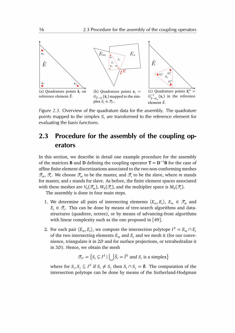
Figure 2.3. Overview of the quadrature data for the assembly. The quadraturepoints mapped to the simplex Si are transformed to the reference element forevaluating the basis functions.
2.3 Procedure for the assembly of the coupling op-erators
In this section, we describe in detail one example procedure for the assemblyof the matrices B and D defining the coupling operator T = D�1B for the case ofaffine finite element discretizations associated to the two non-conforming meshesTm, Ts. We choose Tm to be the master, and Ts to be the slave, where m standsfor master, and s stands for slave. As before, the finite element spaces associatedwith these meshes are Vh(Tm), Wh(Ts), and the multiplier space is Mh(Ts).
The assembly is done in four main steps.
1. We determine all pairs of intersecting elements hEm, Esi, Em 2 Tm andEs 2 Ts. This can be done by means of tree-search algorithms and data-structures (quadtree, octree), or by means of advancing-front algorithmswith linear complexity such as the one proposed in [49].
2. For each pair hEm, Esi, we compute the intersection polytope I E = Em \ Es
of the two intersecting elements Em and Es and we mesh it (for our conve-nience, triangulate it in 2D and for surface projections, or tetrahedralize itin 3D). Hence, we obtain the mesh
TI E =�Si ✓ I E |[ Si = I E and Si is a simplex
where for Si, Sj ✓ I E if Si 6= Sj then Si \ Sj = ;. The computation of theintersection polytope can be done by means of the Sutherland-Hodgman
17 2.3 Procedure for the assembly of the coupling operators
clipping algorithm [130]. Note that the mesh TI E does necessarily has to beexplicitly created, the next step can be performed by treating each simpleximplicitly by only using the intersection polytope connectivity.
3. We generate the quadrature points for integrating in the intersection re-gion I E. This can be done by mapping points from quadrature rules definedon the reference simplex E to each simplex Si.
4. We compute the local element-wise contributions by means of numericalquadrature and assemble the two matrices B and D.
We now focus exclusively on the details of the last two steps, that is on the as-sembly of the operators with respect to a given pair of elements hEm, Esi andtheir intersection I E. We start by choosing a suitable quadrature formula (suchas Gaußian quadrature [127]), with K points {xk}Kk=1 ✓ E and weights {↵k}Kk=1
withPK
k=1↵k = 1. An example quadrature formula is shown in Figure 2.3(a).Then, for each simplex Si:
• We map the quadrature points {xk}k ⇢ E to Si obtaining {xk}k ⇢ Si asshown in Figure 2.3(b).
• We transform {xk}k ⇢ Si ✓ Em \ Es to the reference element for both ele-ments: xm
k = G�1E!Em
(xk) and xsk = G�1
E!Es(xk), where GE!Ei
, i 2 {m, s}, is the
transformation from the reference element E to the element Ei as shownin Figure 2.3(c).
• We set weights
↵0k := ↵k|E||det(rGE!Es(xs
k))| |Si|/ |Es| ,where by |X | for X ✓ Rd we denote the volume of X .
• We compute and add the local contributions to the global coupling matricesas follows
bp,q bp,q +KX
k=1
↵0k p(xsk)�q(xm
k ),
dp,q dp,q +KX
k=1
↵0k p(xsk)✓q(xs
k),
the matrix entries at p, q for B and D respectively, where p, �q, ✓q are basisfunction defined in the reference element. The respective global counter-parts are �p 2 Vh(Em), ✓q 2Wh(Es), and q 2 Mh(Es)which is the Lagrangemultipliers basis associated to Es.
18 2.3 Procedure for the assembly of the coupling operators
Section title
⌦
h1 ⌦
h2
"1 "2
⌦
h2⌦
h1
⌦
h1
⌦
h2
n g
⌦
h1
u
Section title
⌦
h1 ⌦
h2
"1 "2
⌦
h2⌦
h1
⌦
h1
⌦
h2
n g
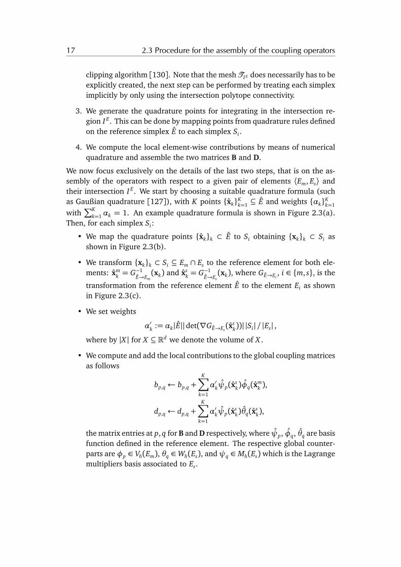
Figure 2.4. Displacement u, surface normal vector n and gap g.
2.3.1 Assembly procedure for two-body contact problems
The use of mortar methods in contact simulations requires, not only a more in-volved selection of candidates, but also a more involved assembly procedure [34].Let us consider a two-body contact problem, between two linear elastic bodies.The two bodies are conveniently denoted as ⌦m ⇢ Rd and ⌦s ⇢ Rd , ⌦m \⌦s = ;.The displacement field u, decomposed into um and u s, is given as the solutionto the boundary value problem
�div�(u) = f in ⌦
u = q on � D
�(u)n = p on � N ,(2.13)
where � is the stress tensor incorporating the material law, n is the outer surfacenormal, ⌦ = ⌦m[⌦s and � = �s[ �m, with �s\ �m = ;, represent the boundary of⌦. With � D we denote the Dirichlet boundary, with � N the Neumann boundaryand with � C the contact boundary, (� D \ � N ) [ (� D \ � C) [ (� N \ � C) = ;. Wecover linearized contact conditions which do not apply to more general non-linear problems. Such conditions are constructed by considering a very specificset of contact directions defined by the normal field on � C
s which leads to thefollowing definition of gap function g : � C
s ! R, with
g(x ) = minx m2� C
m
n(x )T (x m � x ),
and the following non-penetration condition, 8x 2 � Cs
n(x )T (u s(x )� um(y)) g(x ), (2.14)
where y = argminx m2� Cm
n(x )T (x m � x ). We consider a frictionless contact prob-lem, hence on � C the tangential components of the stress are expected to be

19 2.3 Procedure for the assembly of the coupling operators
equal to zero, and the normal component to be less or equal to zero. Figure 2.4provides a visual representation of these quantities.
We discretize ⌦m and ⌦s with respective meshes Tm and Ts. With Vh =V d
h (Tm), W h =W dh (Ts), and Mh = M d
h (Ts), where d corresponds to the spatial di-mension, we denote tensor-product spaces. Let um
h 2 Vh and u sh 2 W h represent
the discete displacement fields in the master and slave mesh respectively.The assembly procedure of the coupling matrices B and D, the weighted gap
block-vector g M 2 M dh (Ts) and weighted normal block-vector nM 2 Mh consists
of the following steps:
1. we determine all the pairs of near surface elements hEm, Esi, Em 2 Tm andEs 2 Ts. We employ the same strategies mentioned in Section 2.3, i.e.,octrees and spatial-hashing, but we enlarge the bounding volumes of thesurface elements by small amounts in both positive and negative normaldirections.
2. Let Es be a planar surface element with normal n, which defines a pro-jection plane. For simplicity we perform our computation in a (d � 1)-dimensional setting. Hence, if d = 3, we compute the affine map G(x ) =Ax + q1, where A = [w , v ,n], where w = q2 � q1, v = q3 � q1,n =(w ⇥ v)/kw ⇥ vk2, and q i, i = 1, . . . , n are the vertices of the element Es.Note that G�1(Es) = E ⇢ Rd�1 is the reference element of the surface ele-ment Es. For the sake of brevity, we denote the set {G(q)},q 2Q, where Qis a set of points, as G(Q). We transform the master surface element andobtain obtaining Em
G = G�1(Em), from which we remove the last compo-nent from all its vertices and obtain the (d � 1)-dimensional orthogonalprojection Em.
We find the intersection I = E \ Em. If I = ; we stop. Otherwise, forthe slave side we compute Is = G( I). For the master side we compute theorthogonal projection of I onto the surface defined by Em
G , the result is thentransformed by G to world coordinates thus obtaining Im.
3. Once we have Is and Im we compute the coupling operators D and B as inthe procedure illustrated in Section 2.3 by following step 3 and 4.
4. We assemble the weighted direction vector and weighted gap vector as
20 2.3 Procedure for the assembly of the coupling operators
follows:
nMp nM
p +KX
k=1
↵0kµp(xsk) · n(xs
k)
g Mp g M
p +KX
k=1
↵0kµp(xsk) · e1 g(xs
k),
where e1 = [1,0, 0]T , µp is the counterpart of µp 2 Mh in the referenceelement, and p 2 Js
C , JsC = { j 2 Ns| supp(µ j)\ �C 6= ;}. The d-dimensional
blocks of vector nM are normalized after assembly.
Note that if p 62 JsC we consider all the associated elements in B, D, nM as zero.
For the gap vector g M we set the entries of p 62 JsC to a suitable large number
⌘ 2 R>0 and to [g Mp · e1,⌘,⌘] otherwise. We consider the indices in Js
C to becontiguous so that we can visualize the results as
B =0 BC
0 0
�, D =
DC 00 0
�,nM =
nC
0
�, g M =
g C
⌘
�.
We compute the coupling operator T = D gB + Id, where D g is the generalizedinverse of D, the gap-vector coefficients g = D gg M , and the block-vector D gnM
which is then normalized block-wise to obtain the block-vector of normals n.Since we have chosen to assign what we call normal component to the first co-
ordinate of each block of the gap vector. In fact we assume, a normal-tangentialcoordinate system (frame of reference) spanned by the mutually orthogonal vec-tors np, t 1
p, t 2p which are respectively the weighted surface normal an the respec-
tive tangential vectors at the node p.Let us consider the following linear system of equations Au = f arising from
our contact problem (2.13). In order to work with the non-penetration conditionwe transform the systems of equation. We do this by means of the Householdertransformation Opp = Id� 2w w T , w = (np + e1)/knp + e1k2, Opp = OT
pp = O�1pp
for p 2 JsC , and by Opp = Id otherwise. We finally write the algebraic formulation
of (2.13) as
OT T ATOu = OT T f ,
u g
where u = OT T u, which we solve by means of any method which handlesinequality constraints, such as projected gauss-seidel, non-linear multigrid, orsemi-smooth Newton methods [138; 107].

21 2.3 Procedure for the assembly of the coupling operators
Input Result Detail
Figure 2.5. Contact simulation between a parallelepiped and a cylinder withautomatically determined contact.
Automatic determination of contact patches
When using the mortar method in contact problems the role of adjacent surfaceelements has to be the same, i.e., if an element is assigned the master role allits adjacent elements can not be assigned the slave role, and vice-versa for anelement with the slave role.
When the slave and master roles are not provided a-priori by the user, theyare determined automatically. An example of such situation is self-contact intransient scenarios. In such cases it is natural to consider the element describingdifferent bodies as part of a unique mesh. A strategy for automatically handlingthis assignment problem is presented in [141]. We describe a more basic strategywhich consists of three main steps.
The first step consists of rejecting pairs of element which are detrimental tothe quality of the discretized non-penetration constraints. One criterion is toreject pairs of elements that have a common node. Another criterion is to rejectpairs of elements for which cos✓ > � , where cos✓ = nT
s nm is the cosine of theangle between the normals ns and nm defined on the slave and master surfaceelements respectively, and � 2 R<0.
The second step consists of identifying which elements are suitable to be as-signed the slave role. An element Es is considered suitable if its area |Es|is ap-proximately equal to the total area of the geometric normal projection
PKk=1 |I k
s |(Section 2.3.1), where K is the number of geometric projections. This step givesus a weighted directed graph C with n vertices, which we call contact graph,where each vertex corresponds to an element, and each edge goes to a validslave candidate Ei to a valid master candidate Ej . We consider the weight ci j
associated to the edge (i, j) of C to be the average gap function from the slave
22 2.3 Procedure for the assembly of the coupling operators
Input Result
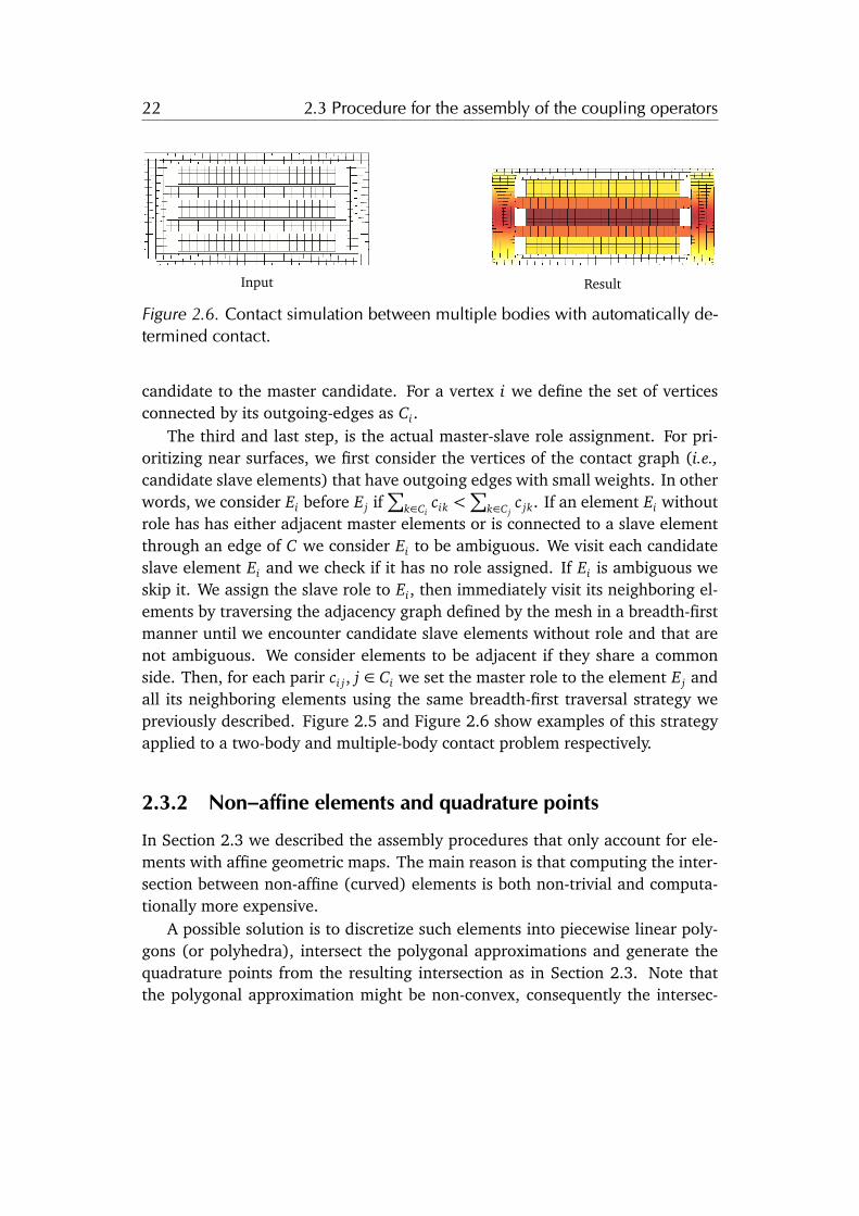
Figure 2.6. Contact simulation between multiple bodies with automatically de-termined contact.
candidate to the master candidate. For a vertex i we define the set of verticesconnected by its outgoing-edges as Ci.
The third and last step, is the actual master-slave role assignment. For pri-oritizing near surfaces, we first consider the vertices of the contact graph (i.e.,candidate slave elements) that have outgoing edges with small weights. In otherwords, we consider Ei before Ej if
Pk2Ci
cik <P
k2Cjc jk. If an element Ei without
role has has either adjacent master elements or is connected to a slave elementthrough an edge of C we consider Ei to be ambiguous. We visit each candidateslave element Ei and we check if it has no role assigned. If Ei is ambiguous weskip it. We assign the slave role to Ei, then immediately visit its neighboring el-ements by traversing the adjacency graph defined by the mesh in a breadth-firstmanner until we encounter candidate slave elements without role and that arenot ambiguous. We consider elements to be adjacent if they share a commonside. Then, for each parir ci j, j 2 Ci we set the master role to the element Ej andall its neighboring elements using the same breadth-first traversal strategy wepreviously described. Figure 2.5 and Figure 2.6 show examples of this strategyapplied to a two-body and multiple-body contact problem respectively.
2.3.2 Non–affine elements and quadrature points
In Section 2.3 we described the assembly procedures that only account for ele-ments with affine geometric maps. The main reason is that computing the inter-section between non-affine (curved) elements is both non-trivial and computa-tionally more expensive.
A possible solution is to discretize such elements into piecewise linear poly-gons (or polyhedra), intersect the polygonal approximations and generate thequadrature points from the resulting intersection as in Section 2.3. Note thatthe polygonal approximation might be non-convex, consequently the intersec-
23 2.4 Space partitioning and ordering
Section titleSection titleSection title
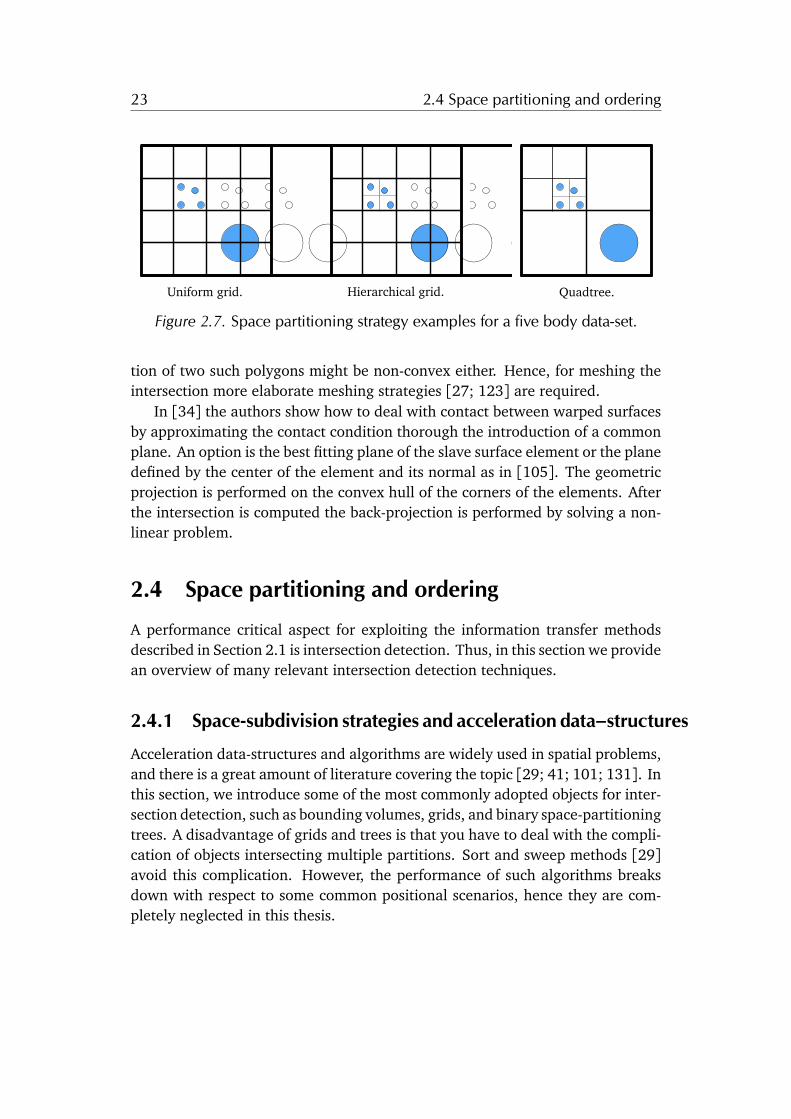
Uniform grid. Hierarchical grid. Quadtree.
Figure 2.7. Space partitioning strategy examples for a five body data-set.
tion of two such polygons might be non-convex either. Hence, for meshing theintersection more elaborate meshing strategies [27; 123] are required.
In [34] the authors show how to deal with contact between warped surfacesby approximating the contact condition thorough the introduction of a commonplane. An option is the best fitting plane of the slave surface element or the planedefined by the center of the element and its normal as in [105]. The geometricprojection is performed on the convex hull of the corners of the elements. Afterthe intersection is computed the back-projection is performed by solving a non-linear problem.
2.4 Space partitioning and ordering
A performance critical aspect for exploiting the information transfer methodsdescribed in Section 2.1 is intersection detection. Thus, in this section we providean overview of many relevant intersection detection techniques.
2.4.1 Space-subdivision strategies and acceleration data–structures
Acceleration data-structures and algorithms are widely used in spatial problems,and there is a great amount of literature covering the topic [29; 41; 101; 131]. Inthis section, we introduce some of the most commonly adopted objects for inter-section detection, such as bounding volumes, grids, and binary space-partitioningtrees. A disadvantage of grids and trees is that you have to deal with the compli-cation of objects intersecting multiple partitions. Sort and sweep methods [29]avoid this complication. However, the performance of such algorithms breaksdown with respect to some common positional scenarios, hence they are com-pletely neglected in this thesis.
24 2.4 Space partitioning and ordering
2.4.2 Bounding volumes
A bounding volume is a closed volume completely containing a set of geomet-ric objects. Testing a bounding volume for intersections has to be significantlycheaper than testing the contained objects. Commonly used bounding volumesare bounding-spheres and convex-hulls. In this thesis we cover exclusively thediscrete oriented polytope (DOP) and the axis-aligned bounding-box (AABB).The k-DOP is a discrete oriented polytope described as the intersection of k half-spaces, see Figure 2.8. The AABB can be considered as a special case of the k-DOPwhere the half-space orientations are given by the canonical basis vectors. Morespecifically, a k-DOP B is defined as a set of k normal vectors [b1, b2, . . . , bk]and signed distances from the origin of the respective cutting planes. We de-note the minimum distances as Bm = [Bm
1 , Bm2 , . . . , Bm
k ] and the maximum dis-tances as BM = [BM
1 , BM2 , . . . , BM
k ]. The k-DOP of a set of points Q is computed asBm
i =minq2Q bi · q and BMi =maxq2Q bi · q , i = 1, . . . , k. For a pair of k-DOPsA
andB if9i=1,...,k AM
i < Bmi _ BM
i < Ami , (2.15)
is satisfied, then there is no intersection.
2.4.3 Spatial hashing
Spatial hashing data-structures, such as implicit grids, allow having constantcomputational time complexity spatial queries for several applications, such as3D parameterized textures, 3D painting, collision and intersection detection.Here, we focus on the latter application. There are several strategies for per-formance reliable spatial hashing, for computations both on CPU and GPU, suchas perfect hashing [84].
For uniformly or quasi-uniformly sized and distributed data, spatial hashingprovides the fastest way of detecting intersections. The simplest spatial-hashingdata-structure is a uniform implicit grid, which we refer to as hash-grid. Werecall the definitions of k-DOP and AABB introduced in Section 2.4.2. The hash-grid is constructed by dividing each dimension k of the axis-align bounding-boxB = [Bm,BM] in
nk =
6664⇠
12
ÅN2
ã1/s⇡ BMk � Bm
k
minl=1,...,s
(BMl � Bm
l )
7775
intervals which creates n =Qs
k=1 nk cells, where Bmk , BM
k denote the k-th com-ponents of the respective vectors, b·c is the floor operator, and d·e is the ceiling

25 2.4 Space partitioning and ordering
operator. The hash function is of the form
h(x ) =dX
k=1
ÅIk(x )
dY
l=k+1
nlã
,
whereIk(x ) =
ö(xk � Bm
k )/(BMk � Bm
k ) · nkù
describes the grid-index at dimension k. The cost of evaluating the hash functionh only depends on the dimension d. If we fix d, the computational time complex-ity of evaluating h is constant. We build for each cell of the grid a list L of possiblyintersecting objects by exploiting h. This indexing process has O (n|L|max) where|L|max is the maximum number of objects pointed by a cell. In order to index apolytope E (e.g., an element of a mesh) we use its bounding-box B for identi-fying which cells is intersecting. We compute I m = I (Bm) and I M = I (BM)which are respectively starting and ending tensorial indices of a range of cells ofthe grid. We iterate over the cells within this range and we append E to the listof the corresponding table entry. Elements generally intersects more than onecell, hence when we compute the list of intersections for some element, we flagthe elements that have been encountered in any of the visited cells, in order toavoid adding them twice in the intersection list. Once this list is complete weremove the flags from its elements.
The performance of the hash-grid is dependent on |L|max, which can grow(unnecessarily) in scenarios where there is high variability of element sizes andpositions.
Hierarchical grids allow to treat data with different size more efficiently thansimple uniform grids. A hierarchical grid is composed by a set of nested gridsorganized by levels. The main difference with space-partitioning trees (Sec-tion 2.4.4) is that there is no root. Hierarchical grids are extensively explainedin [41].
2.4.4 Space-partitioning trees and bounding volume hierarchies
Binary space partitioning trees (BSP trees) recursively subdivide space into con-vex subsets. This subdivision is done by means of hyper-planes which can haveany orientation. A special case of BSP trees, where the hyper-planes have the ori-entation of the canonical basis vectors, are kd-trees, quadtrees and octrees. Thelatter ones are used to partition space by recursively subdividing it with eitherfour quadrants for the quadtree, or eight octants for the octree. From now onwe refer to quadrants and octants as cells. This partitioning strategy allows for
26 2.4 Space partitioning and ordering
Overview. k-DOP for one process. k-DOP for another process
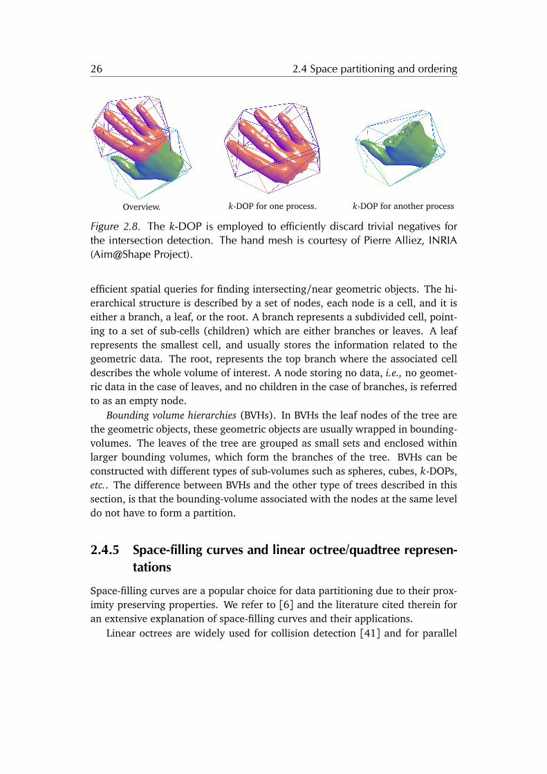
Figure 2.8. The k-DOP is employed to efficiently discard trivial negatives forthe intersection detection. The hand mesh is courtesy of Pierre Alliez, INRIA(Aim@Shape Project).
efficient spatial queries for finding intersecting/near geometric objects. The hi-erarchical structure is described by a set of nodes, each node is a cell, and it iseither a branch, a leaf, or the root. A branch represents a subdivided cell, point-ing to a set of sub-cells (children) which are either branches or leaves. A leafrepresents the smallest cell, and usually stores the information related to thegeometric data. The root, represents the top branch where the associated celldescribes the whole volume of interest. A node storing no data, i.e., no geomet-ric data in the case of leaves, and no children in the case of branches, is referredto as an empty node.
Bounding volume hierarchies (BVHs). In BVHs the leaf nodes of the tree arethe geometric objects, these geometric objects are usually wrapped in bounding-volumes. The leaves of the tree are grouped as small sets and enclosed withinlarger bounding volumes, which form the branches of the tree. BVHs can beconstructed with different types of sub-volumes such as spheres, cubes, k-DOPs,etc.. The difference between BVHs and the other type of trees described in thissection, is that the bounding-volume associated with the nodes at the same leveldo not have to form a partition.
2.4.5 Space-filling curves and linear octree/quadtree represen-tations
Space-filling curves are a popular choice for data partitioning due to their prox-imity preserving properties. We refer to [6] and the literature cited therein foran extensive explanation of space-filling curves and their applications.
Linear octrees are widely used for collision detection [41] and for parallel
27 2.4 Space partitioning and ordering
0
1
2
3
level
a
a
b
b
c
c
d
d
e
e
f
h
g
f
h
g
root
depth
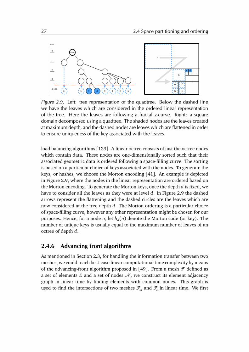
Figure 2.9. Left: tree representation of the quadtree. Below the dashed linewe have the leaves which are considered in the ordered linear representationof the tree. Here the leaves are following a fractal z-curve. Right: a squaredomain decomposed using a quadtree. The shaded nodes are the leaves createdat maximum depth, and the dashed nodes are leaves which are flattened in orderto ensure uniqueness of the key associated with the leaves.
load balancing algorithms [129]. A linear octree consists of just the octree nodeswhich contain data. These nodes are one-dimensionally sorted such that theirassociated geometric data is ordered following a space-filling curve. The sortingis based on a particular choice of keys associated with the nodes. To generate thekeys, or hashes, we choose the Morton encoding [41]. An example is depictedin Figure 2.9, where the nodes in the linear representation are ordered based onthe Morton encoding. To generate the Morton keys, once the depth d is fixed, wehave to consider all the leaves as they were at level d. In Figure 2.9 the dashedarrows represent the flattening and the dashed circles are the leaves which arenow considered at the tree depth d. The Morton ordering is a particular choiceof space-filling curve, however any other representation might be chosen for ourpurposes. Hence, for a node n, let hd(n) denote the Morton code (or key). Thenumber of unique keys is usually equal to the maximum number of leaves of anoctree of depth d.
2.4.6 Advancing front algorithms
As mentioned in Section 2.3, for handling the information transfer between twomeshes, we could reach best-case linear computational time complexity by meansof the advancing-front algorithm proposed in [49]. From a mesh T defined asa set of elements E and a set of nodes N , we construct its element adjacencygraph in linear time by finding elements with common nodes. This graph isused to find the intersections of two meshes Tm and Ts in linear time. We first

28 2.5 Parametrizations and finite element discretizations
find a pair of intersecting elements {Em, Es}. We compute the intersection anddetermine if Em is also a viable candidate for the neighbors of Es. Then, we usethe adjacency graph of Em to test the neighboring elements for intersections withEs. We repeat this operation until there are no elements intersecting Es and wemark Es as resolved, and we move to the neighbors of Es and repeat.
In spite of the aforementioned advantages of this approach, we choose tree-search algorithms. Although the advancing-front algorithm in the best case haslower computational time complexity bound (O (n) instead of O (n log(n)), wheren is the size of the input), it does have high hidden additional requirementsin terms of computational cost. For instance, it requires information on whatmeshes or partitions need to be intersected with each other, and to determineeach starting couple of intersecting elements. Particularly in parallel environ-ment with arbitrarily distributed meshes this might not be trivial, or even notefficient. Additionally, with tree-search algorithms we can allow more use cases,as mentioned in the introduction of this thesis, without having to change oursearch strategy.
2.5 Parametrizations and finite element discretizations
The finite element method allows simulating physical phenomena while repre-senting complex geometric objects by means of meshes. Such geometric objectsare complex geometric descriptions which are generated by computer aided de-sign (CAD) software, captured from real life objects or organisms (e.g., 3D scans,MRI, etc.), and need to represented in a sufficiently accurate way. This is the casebecause the accuracy of the geometric representation influences the approxima-tion error of the discrete solution of a partial differential equation.
The influence of accuracy of the geometric representation on the approxi-mation error has been studied for curved boundary of iso-parametric discretiza-tions [26; 114; 115] and for contact problems [75]. More recent literature fo-cuses on numerical studies for different approximation spaces [15; 14], and el-liptic and Maxwell problems [140].
During a simulation the approximation space might not be descriptive enoughto represent the solution. This problem is usually solved by means of adaptive re-finement strategies, such as h-refinement [16; 18] and p-refinement [95]. Whenusing such strategies, a higher resolution at the boundary should be accompa-nied by a better approximation of the original surface [37]. However, due tothe one-way connection between geometric information and simulation envi-ronment, the adaptive refinement is rarely accompanied by an increase in the
29 2.5 Parametrizations and finite element discretizations
accuracy of the shape. In other words, the mesh is generated within a modelingsoftware and used in simulation environments without considering the originalsurface, preventing a better surface approximation.
Iso-geometric analysis (IGA) [67] allows to overcome this limitation by work-ing directly with the geometric description provided by CAD software, such asnon-uniform rational B-splines (NURBS). However, IGA is subject to several chal-lenges such as the treatment of non-watertight surfaces, local refinement andtopological flexibility [87]. Moreover, IGA approximations, similarly to manymesh-free methods, leads to complications in the imposition of essential bound-ary conditions, which can be either imposed in a weak sense [11], or least-squares satisfied in the strong sense [67].
Additionally, when dealing with three-dimensional shapes, CAD models usu-ally describe only the boundary. Creating a NURBS volume parameterization isa complex task, for which many different approaches exits. For instance, someof them require particular shapes [1], need special geometric information [93],or do not reproduce the surface exactly [85].
An alternative to IGA is the NURBS-enhanced finite element method (NE-FEM) [124] that allows exploiting CAD geometries to describe exactly the bound-ary of the geometry. However, this method requires creating a parameterizationmesh, and a special handling of the boundary, which according to [124] is stillan open problem.
Another challenge regards geometric multigrid methods which require a hier-archy of nested spaces for optimal convergence [57; 22]. Such requirement canbe satisfied by generating the hierarchy by refining a coarse mesh representationof the shape. However, such refinement cannot improve the shape accuracy. Analternative approach [35] is to employ a parameterization such as transfinite in-terpolation [110; 111] and to build nested hierarchies in the parameterizationdomain. However, transfinite interpolation requires a surface parametrization,a specific parametrization domain, and it is not guaranteed to be bijective forgeneral polytopes.
2.5.1 Composite mean value mappings
To the best of our knowledge only the composite mean value mappings [121]allow creating smooth-bijective mappings between polytopes, such as polygonsor polygonal meshes. Convenient properties of such mappings are that they canbe evaluated point-wise, are provided in closed form, and are C1 in the interior
30 2.5 Parametrizations and finite element discretizations
b0 =nX
j=1
�0j q
0.5i b0.5 =
nX
j=1
�0.5j q1
j
b = b0.5 � b0
⇥0 ⇥0.5 ⇥
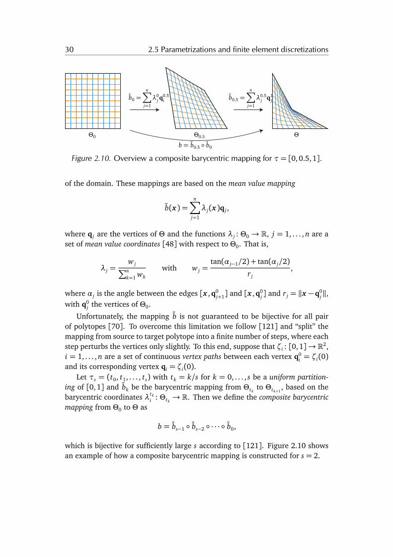
Figure 2.10. Overview a composite barycentric mapping for ⌧= [0,0.5, 1].
of the domain. These mappings are based on the mean value mapping
b(x ) =nX
j=1
� j(x )q j,
where q j are the vertices of ⇥ and the functions � j : ⇥0 ! R, j = 1, . . . , n are aset of mean value coordinates [48] with respect to ⇥0. That is,
� j =wjPn
k=1 wkwith wj =
tan(↵ j�1/2) + tan(↵ j/2)rj
,
where ↵ j is the angle between the edges [x ,q0j+1] and [x ,q0
j ] and rj = kx �q0j k,
with q0j the vertices of ⇥0.
Unfortunately, the mapping b is not guaranteed to be bijective for all pairof polytopes [70]. To overcome this limitation we follow [121] and “split” themapping from source to target polytope into a finite number of steps, where eachstep perturbs the vertices only slightly. To this end, suppose that ⇣i : [0,1]! R2,i = 1, . . . , n are a set of continuous vertex paths between each vertex q0
i = ⇣i(0)and its corresponding vertex qi = ⇣i(0).
Let ⌧s = (t0, t1, . . . , ts) with tk = k/s for k = 0, . . . , s be a uniform partition-ing of [0,1] and bk be the barycentric mapping from ⇥tk
to ⇥tk+1, based on the
barycentric coordinates �tki : ⇥tk
! R. Then we define the composite barycentricmapping from ⇥0 to ⇥ as
b = bs�1 � bs�2 � · · · � b0,
which is bijective for sufficiently large s according to [121]. Figure 2.10 showsan example of how a composite barycentric mapping is constructed for s = 2.
31 2.5 Parametrizations and finite element discretizations
2.5.2 Efficient computation of the Jacobian matrix of the com-posite mean-value mapping
This section provides all derivations for efficiently computing the Jacobian Jb ofthe 3D mean value mapping b [73]. To compute Jb we first need the formula forthe partial derivative of the 3D mean value mapping of a point x ,
b(x ) =nX
i=1
�i(x )q0i =
nX
i=1
wi(x )Pnk=1 wk(x )
q0i ,
where wi are the mean value weights [73] and q0i are the vertices of ⇥0. We first
compute for each triangle T = [q01,q0
1,q03] the quantities
dj = kq0j � xk, v j =
q0j � x
dj
with gradients
rdj =�v j
d j, Jv j
= djId+ v j (rdj)T
for j = 1, 2,3. If x lies on a vertex of the source polyhedron, then we know thatthe image of x is that vertex. Moreover, the function is only C0 at the vertices,hence its gradient is not defined.
Then, we compute
rj =«
4� l2j , ✓ j = 2 arcsin(l j/2), r✓ j = 2
(Jv j+1� Jv j�1
)(v j+1 � v j�1)
l j r j, (2.16)
where l j = kv j+1 � v j�1k, h = (✓1 + ✓2 + ✓3)/2, and rh = (r✓1 +r✓2 +r✓3)/2.If x is inside T , then h is equal to ⇡, and the image of x is given by the two-dimensional barycentric coordinates of that triangular face.
For efficiency reasons, we pre-compute
s✓ j= sin(✓ j) =
l j r j
2, c✓ j
= cos(✓ j) = 1� l2j
2,
shj= sin(h� ✓ j) =
l1l2l38� l j r j+1rj�1
8+
3X
k=1,k 6= j
lk rk+1rk�1
8,
sh = sin(h) = � l1l2l38+
3X
k=1
lk rk+1rk�1
8.
32 2.5 Parametrizations and finite element discretizations
Note that the terms in the sums appear multiple times, hence we cache them.Instead of evaluating the cosines, we exploit the trigonometric identities to com-pute them from the sines, using exclusively square roots, which are much fasterto compute. For instance, cos(⇤) = �p1� ⇤2, where the sign � is computed bychecking if the parameter h lies in the positive or negative region. We then com-pute
cj = 2Ncj
Dcj
� 1= 2shshj
s✓ j�1s✓ j+1
� 1, s j = sign(det([v1,v2,v3]))«
1� c2j ,
the corresponding gradients
rcj = 2Å chrhshj
+ shchj(rh�r✓ j)
Dcj
� Ncjc✓ j+1r✓ j+1
s✓ j�1sin2
✓ j+1
� Ncjc✓ j�1r✓ j�1
s✓ j+1sin2
✓ j�1
ã,
and
rs j = �rcj c j
s j.
If x lies in the same plane as the triangle T and x 62 T , then at least one of thethree s j = 0. In this case, T does not contribute to the computation of wi andhas to be skipped. Otherwise, we compute the mean value weight
wj =Nwj
Dwj
=✓ j � cj+1✓ j�1 � cj�1✓ j+1
djs j+1s j�1
and its gradient
rwj =r✓ j �rcj+1✓ j�1 � cj+1r✓ j�1 �rcj�1✓ j+1 � cj�1r✓ j+1
Dwj
� wj
Årdj
dj+
c✓ j+1r✓ j+1
s✓ j+1
+rs j�1
s j�1
ã.
Finally, we aggregate the local weights and gradients
w=nX
i=1
wi, rw=nX
i=1
rwi,
and compute the Jacobian matrix of the barycentric mapping b,
Jb =nX
i=1
q0i
Årwi + birww
ãT
.
33 2.6 Software libraries and tools for scientific computing
The composite barycentric mapping and its gradient are computed in parallelfor each evaluation point as
b = bM � . . . � b2 � b1, rb =r bM( bM�1 � . . . � b2 � b1) · . . . ·r b2( b1) ·r b1.
We modified the algorithm proposed in [73] in order to avoid computing trigono-metric functions. In fact, our adaptation contains only the computation of thethe arc-sine in (2.16), which is unavoidable because of the use of ✓ .
2.6 Software libraries and tools for scientific com-puting
As new technologies arise, scientific-computing software libraries need to be con-stantly updated or rewritten. For instance, the advent of GPGPU (general pur-pose graphics processing units) induced new programming paradigms and newlanguages such as CUDA [99] and OPENCL [74], which led to the creation ofnew software libraries such as CUBLAS [100] and VIENNACL [117]. Keeping upwith such new technologies may cause small or significant changes in the code ofapplications such as non-linear solution strategies, finite element analysis, anddata-analysis. However, the related high-level algorithms implemented in theapplication code should not have to change.
For this reason, one solution is to develop on top of a portable interface thatfits many current and possibly future requirements (e.g., PETSc [7] and TRILI-NOS [58]). For instance, software libraries such as DEAL.II [8], LIBMESH [76],and MOOSE [50] rely on high level abstractions on top of existing linear alge-bra and non-linear solution strategies codes, and allow choosing the underlyingimplementation in a rather transparent way.
An alternative solution is exploiting scripting facilities for completely decou-pling the application behavior from its actual implementation. This solution hasthe advantage of hiding the complexity of parallel software to which the aver-age, casual or opportunistic [19], user is not supposed to be exposed. The ideais that the scripting code is translated to behavior which is implemented in an-other lower-level language. This enables users to write few lines of very power-ful code without the overhead of learning how to use complex parallel scientificcodes. A very specific form of scripting language is usually referred to as do-main specific language (DSL). This specificity, while reaching the aforementionedobjectives, has a twofold advantage. First, it enables a simple description of aspecific problem since most implementation details can be hidden. Second, it al-lows exploiting complex functionalities and performance critical optimizations.
34 2.7 Chapter conclusion
Notable examples related to finite element softwares, are FENICS’s unified formlanguage [88; 112], FREEFEM++ [71], and LISZT [31].
In DSLs lower-level abstractions are purposefully inaccessible because the ac-tual algorithms are implemented in a different language, such as C++. This isa problem when a DSL misses a functionality, since adding it would require ac-cessing the underlying back-end which may be either closed source or very com-plex. In contrast, embedded domain specific languages (eDSL) (e.g., CULA [68],FEEL++ [104], OPENFOAM [135], SUNDANCE [90], VIENNAFEM [118]) uses thesame language and compiler for both the “scripting” layer and the implementa-tion of the back-end. For this reason, eDSLs have the opportunity to provide theright balance between abstraction and direct access to the back-end data-typesand algorithms.
2.7 Chapter conclusion
In this chapter we first introduced the related work. We covered the variationaltransfer of discrete fields and provided detailed explanations on how to imple-ment it for both volume coupling and contact problems in a serial environment.Then, we briefly touched the subject of volume parameterizations, their impli-cations in finite element work-flows and our volume parameterization of choice:mean-value mappings. Finally, we provided an overview of the current trends inthe development of scientific software. The topics we covered impact the work-flow and structure of finite element softwares and open opportunities for sim-ulating on more accurate geometric descriptions, more automation in couplingcomplex problems, and overall flexibility and usability.
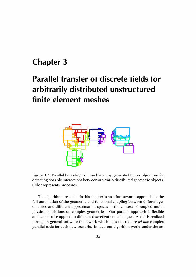
Chapter 3
Parallel transfer of discrete fields forarbitrarily distributed unstructuredfinite element meshes
Figure 3.1. Parallel bounding volume hierarchy generated by our algorithm fordetecting possible interections between arbitrarily distributed geometric objects.Color represents processes.
The algorithm presented in this chapter is an effort towards approaching thefull automation of the geometric and functional coupling between different ge-ometries and different approximation spaces in the context of coupled multi-physics simulations on complex geometries. Our parallel approach is flexibleand can also be applied to different discretization techniques. And it is realizedthrough a general software framework which does not require ad-hoc complexparallel code for each new scenario. In fact, our algorithm works under the as-
35

36 3.1 Parallel pipeline
sumption that we might have multiple meshes arbitrarily decomposed, arbitrarilydistributed, and their relation based on spatial information is not known.
However, it is imporant to note that in cases where the location informationis trivially and globally accessible, for instance with Cartesian grids or structuredmeshes, our approach is not optimal. Our algorithm is designed as a generalblack-box solution, hence it might not be as efficient as a reduced variant specif-ically designed for Cartesian grids.
In Section 3.1, we provide an overview of the parallel algorithmic pipeline.In Section 3.2, we present a parallel spatial search algorithm and the necessarydata-structures (Figure 3.1) for finding near or intersecting geometric objects,such as the mesh surface or volume elements. In Section 3.3, we present how theoperator can be represented within the code, and how we can solve and handleall the relationships in one pass of the algorithm. In Section 3.4, we discuss whatexisting software tools we can use in order to implement the approach.
3.1 Parallel pipeline
The pipeline of our parallel approach to surface and volume projections consistsof two main phases, a search phase and a compute phase. Each process, from itslocal knowledge about the data, gathers a minimal amount of information allow-ing it to determine its dependencies and executes the assembly of the transferoperator in a possibly balanced way. We will use the following terminology inorder to refer to different roles that a process can have with respect to data andcomputation: owner process, which is a process owning a specific set of data be-fore starting our algorithm and the related output at the end of our algorithm;worker process, which is a process performing computation on data which mightor might not be its own. Our two-stages parallel pipeline can be summarized asfollows:
1. Parallel intersection/proximity detection, explained in Section 3.2. A set ofinput meshes distributed arbitrarily to different owner processes is used asan input to our parallel tree-search algorithm. The tree-search algorithmthen creates list of candidate-matching-element-pairs. This list of candi-date pairs is used to identify near or intersecting objects (see Figure 3.2),and it is partitioned evenly among the processes for computation.
2. Parallel operator assembly, explained in Section 3.3. This phase is dividedinto a local and a global part. In the local part, we compute geometricprojections/intersections and generate meshes on the intersections for the
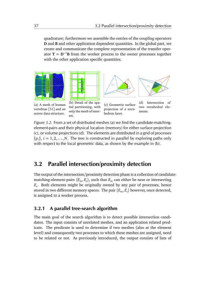
37 3.2 Parallel intersection/proximity detection
quadrature; furthermore we assemble the entries of the coupling operatorsD and B and other application dependent quantities. In the global part, wecreate and communicate the complete representation of the transfer oper-ator T = D�1B from the worker process to the owner processes togetherwith the other application specific quantities.
p0
p1
p1
p0
(a) A mesh of humanvertebrae [51] and anoctree data-structure.
(b) Detail of the spa-tial partitioning, withonly the mesh of inter-est.
(c) Geometric surfaceprojection of a tetra-hedron facet.
(d) Intersection oftwo tetrahedral ele-ments.
Figure 3.2. From a set of distributed meshes (a) we find the candidate-matching-element-pairs and their physical location (memory) for either surface projection(c), or volume projections (d). The elements are distributed in a grid of processes{pi}, i = 1,2, . . . , N . The tree is constructed in parallel by exploring paths onlywith respect to the local geometric data, as shown by the example in (b).
3.2 Parallel intersection/proximity detection
The output of the intersection/proximity detection phase is a collection of candidate-matching-element-pairs hEm, Esi, such that Em can either be near or intersectingEs. Both elements might be originally owned by any pair of processes, hencestored in two different memory spaces. The pair hEm, Esi however, once detected,is assigned to a worker process.
3.2.1 A parallel tree-search algorithm
The main goal of the search algorithm is to detect possible intersection candi-dates. The input consists of unrelated meshes, and an application related pred-icate. The predicate is used to determine if two meshes (also at the elementlevel) and consequently two processes to which these meshes are assigned, needto be related or not. As previously introduced, the output consists of lists of
38 3.2 Parallel intersection/proximity detection
intersection-candidate pairs relating geometric objects (e.g., tetrahedra , hexa-hedra) on pairs of processes. For sake of simplicity and clarity, let us assume thatwe have only one mesh or a subset of one mesh per process (for details aboutmultiple meshes see Section 3.2.3). Efficient collision detection algorithms areusually divided into two phases, broad and narrow. In the broad phase, the testsare conservative and fast in order to reject trivial negatives. In the narrow phase,collision tests are exact and the actual intersection data is computed. We followa similar structure to illustrate our strategy, hence we divide it in three maindetection phases: broad, middle, and narrow.
Broad-phase detection
The main purpose of this phase is to eliminate, in the cheapest way possible, anytrivial negative for our search, and the identification of which processes are re-lated and which are not. In each process, we locally construct bounding volumedata: an AABB and a k-DOP, as introduced in Section 2.4.1. We exchange amongall processes the bounding volume data together with application predicate data.We are now able to discard trivial negatives and have pair-wise relations betweenprocesses. We call two processes related if they have a common non-empty par-tition of space accepted by the application predicate. With the union of all localAABBs, we can create a global AABB which will be the root of our tree search.Note that at this point we might already have created a sparse communicationgraph, hence allowing independent and specific point-to-point communicationbetween related processes. A simple example is depicted in Figure 3.3. In Fig-ure 3.3(a) we have one mesh per process, T1 for process p1 and T2 for process p2,and we want to determine the possible contact boundary between them. At theend of the broad-phase detection the overall knowledge of process p1, as shownin Figure 3.3(b), consists of its local information, the global bounding box andthe bounding box associated with process p2 and T2. This information allowsus to reduce the amount of data to be considered substantially. In case of morecomplex set-ups (e.g., concave objects) this is not always the case. Hence, a re-fined search might be necessary, which brings us to the middle-phase detectionalgorithm.
Middle-phase detection
The main purpose of this phase is to detect, on a finer scale, which non-emptypartitions of space exist and are shared between different processes. In order todo that, we build a lookup table, where each partition of interest is mapped to
39 3.2 Parallel intersection/proximity detection
all processes where this partition is non-empty. We realize this by performingmultiple simultaneous breadth-first traversals of the tree (quadtree, octree, or n-dimensional generalization). More precisely, we perform a breadth-first traversalfor each pair of related processes. A traversal must be simultaneous between apair of related processes, however the other traversals in both processes can beconsidered concurrently, hence allowing for additional parallelism. The traver-sals can be performed by taking advantage of asynchronous communication (e.g.,when implementing the algorithm with the MPI standard), i.e., by opportunisti-cally advancing a traversal whenever new information is received by any otherprocess.
We start with the partition of space described by the root of the tree, which isthe same for every process (constructed in the phase described in Section 3.2.1).Local to each process p, we have to consider the following objects:
• For the nodes of the tree, a lightweight representation is needed in order tobe exchanged after each iteration of the algorithm, and its essential formcomes with the following data: the node-id; a first boolean flag, whosevalue is true when the node is empty and false otherwise; a second booleanflag, whose value is true if it is a leaf node and cannot be refined (hencechanged into a branch), and false otherwise. The refinement of the searchcan be controlled by application specific predicates.
• A queue Qpq for each related process q, where Qpq ⌘Qqp (i.e., equivalent).The queue Qpq = [n0, n1, . . . , nk] contains the next k nodes of the tree tobe visited for the simultaneous traversal of the process pair {p, q}. In orderto perform a breadth-first traversal, the queue is treated with a first in firstout (FIFO) policy, hence we push to the back of the queue and pop fromthe front. With Qpq(i) we describe the ith element from the front of thequeue.
• We define the lightweight representation of Qpq as the queue Qpq, whoseelements are lightweight node representations. This representation is cre-ated by process p, and communicated to process q.
• A list Lpq of non-empty nodes, such that Lpq ⌘ Lqp. These nodes are eitherleaves or branches, and identify where the various paths of the traversalstop.
Each process p performs the following operations at each level l for each relatedprocess q, q 6= p:
40 3.2 Parallel intersection/proximity detection
• If l = 0, we push the children of the root into queue Qpq, and we continueto the next level.
• If l > 0, we create Qpq from Qpq and we send it to process q, and we receiveQqp from q.
• We process each pair ni = Qpq(i), ni = Qqp(i), where i = 1, . . . , m and m isthe number of elements in Qqp and Qqp (note that Qqp contains exclusivelynodes at level l). If ni or ni are empty, we move on to the next pair. Ifeither ni or ni are leaves and cannot be refined to branches, we add ni toLpq. Otherwise, if ni is a leaf, then we refine ni to a branch, and we pushthe children of ni into Qpq. All m nodes which we considered are poppedfrom Qpq. It can be observed that this part of the procedure is and needs tobe symmetric with respect to p and q, ensuring consistent representationsof the traversal between related processes.
• If Qpq is empty, we end the simultaneous traversal with respect to the pairp and q. Additionally, if Lpq is also empty, we consider p and q to be unre-lated.
We can now construct the lookup table Lp from p to any related process q bygathering the information in all Lpq. For each node of the local tree we identifyin which other processes the same (remote) node exists and how much data itcontains. This information can be used to balance the narrow-phase search.
An example execution of the middle-phase detection algorithm is illustratedin Figure 3.4. Here, we can see how the quadtree structure is updated after eachiteration, until we obtain a small partition of space containing all the data ofinterest.
Linearization and load-balancing
Generally, the middle-phase detection generates an output that gives rise to anunbalanced narrow-phase search. For this reason, before entering the narrow-phase detection phase, we redistribute the work. Hence, we first generate a linearrepresentation of the tree with local Morton ordering, then we identify the pair-wise matching nodes by means of the lookup table resulting from Section 3.2.1,balance and redistribute the node and related data accordingly.
With the set Sp, we define the data storage (e.g., the mesh) for each elementE 2 Sp owned by process p. We now construct a re-purposed linear representa-tion of the tree as a piecewise-ordered set of nodes Z . We recall the lookup tableand its entries Lpq defined in Section 3.2.1. A node n 2 Lpq and a node m 2 Lpr ,

41 3.2 Parallel intersection/proximity detection
⌦
h1 ⌦
h2
"1 "2
⌦
h1 ⌦
h2
Overview. Knowledge of p1. Knowledge of p2.
Figure 3.3. Parallel tree-search: result of the broad-phase detection algorithm.The objective is detecting near/intersecting elements between meshes T1 andT2. Here, we can see the respective polygonal domains ⌦h
1 and ⌦h2. owned
respectively by process p1 and p2. The roots’ bounding volumes and the usermeta-data are exchanged. In case of surface projections, in order to detect nearsurfaces, the faces are considered to be blown-up in normal direction by a func-tion "i : ⌦h
i ! R.
⌦
h1 ⌦
h2 ⌦
h1 ⌦
h2
First iteration. After the information of the nodes at level 1 has been exchanged between p1 andp2, both processes know which partitions are of interest and which are not. The nodes in theshaded area will be refined, and the children exchanged.
⌦
h1 ⌦
h2 ⌦
h1 ⌦
h2
Second iteration. By repeating the procedure applied in the first iteration, the are of interest hasbecome smaller.
⌦
h1 ⌦
h2 ⌦
h1 ⌦
h2
Last iteration. The highlighted quadrants contain the data of interest. This quadrants are refer-enced in the lookup tables L1,2 and L2,1 introduced in Section 3.2.1.
Figure 3.4. Parallel tree-search: the middle-phase detection algorithm. Localknowledge of a pair of processes. Left column: overview. Middle column:knowledge of p1. Right column: knowledge of p2. For each iteration, the areaof interest, hence the focus of the search, is marked by the shaded area.
42 3.2 Parallel intersection/proximity detection
with hd(n) = hd(m), hence with same key, are considered to be the same nodeif and only if q = r. Let Bn be the AABB of node n and BE of element E, we saythat n contains E if and only if BE\Bn 6= ;. Let Np(n), be the number of elementscontained by node n for process p, hence E 2 Sp is counted if contained by n.Let C(n) := Cpq(n) be a cost function for node n and the pair of processes p andq, for instance Cpq(n) = Np(n)Nq(n) or Cpq(n) = Np(n) + Nq(n). Since node n isboth in Lpq and in Lqp, for each process p we create a new set, our unbalancedlocal work set
Up =[pq
Lpq.
Locally to each process p, for each node n 2 Up we generate its key hd(n) andsort Up according to the node keys, generating the ordered set Up sorthd
(Up). For nodes with equal key, the rank of their associated remote process is usedas secondary key, hence for n, m 2 Up, with n 2 Lpq and m 2 Lpr , such thathd(n) = hd(m), n comes before m if q < r. Note that d is the depth of the globaltree hence d =maxp(dp) where dp is the local depth for process p.
In a slight abuse of notation let us define the distributed piecewise-orderedset as a concatenation of the local ones, hence U = U1 � U2 � . . . � UP whereP is the number of processes, and � is the concatenation operator. With U(i),where i 2 {1,2, . . . , |U |}, we define the i-th element of U , hence the i-th node.With X ( j) = X ( j � 1) + C(U( j � 1)), where j 2 {1, 2, . . . , |U |+ 1} and X (1) = 0,we define the cumulative cost at node U( j). With an exclusive scan operationwe can compute X . We now know the total cost CT = X (|U |+ 1), average costCA = bCT/Pc and remainder CR = mod(CT , P).
Our goal is to distribute the nodes and their content such that each processp will have a balanced local work set Zp such that the associated cost CZp
=Pn2Zp
C(n) is as near as possible to CA.For each process p in parallel:
• For each process q:
– Compute lower bound lq and upper bound uq. If q CR then
lq (q� 1)(CA+ 1) and uq q(CA+ 1),
otherwise
lq (q� 1)CA+ CR and lu qCA+ CR.
– If lq Xp(i) uq, i = 1, 2, . . . , |Xp| then append Up(i) to Z pq . With Z p
qwe denote a local-to-p partial representation of the balanced work setZq, which will have to be sent to q in a second moment.

43 3.2 Parallel intersection/proximity detection
b
c
d
e
f h
g
a
d
h
g
a
b
c
d
e
f
p1
p0
p2
d
d
d
d
d
d
p0 p1 p2
Figure 3.5. A circle represent a node of the linear tree. For each process pi withi 2 {1,2, 3}, we see a row of nodes. Each row represent a local view of thelinearized tree depicted in Figure 2.9. Each column represents matching nodepairs. The work is partitioned along the space filling curve among the differentprocesses pi as shown by the grouping on the bottom.
Note that the data associated with each node n 2 Z pq is either on one or two
different processes. With Dpr(q), we describe the set of dependencies which arenon local to p, owned by r and destined to the worker process q. This impliesthat in order to be able to completely construct Zq, p has to send Dpr(q) to rwhich then can construct Z r
q . Now both owner processes p and r can send thecorrect data to the worker q to construct Zq. Hence, we have now constructedZ = Z1�Z2�. . .�ZP . With n 2 Zp we are able to directly access the data containedby n from process p.
Narrow-phase detection
The main purpose of this phase is to obtain the list of element pairs that arematching (intersecting), and related intersection data which is then to be usedfor quadrature as seen in Section 2.3. For each node of our linear tree we havetwo sets of elements which have to be matched with each other. We are searchingmatching-pairs at each node of the tree independently. A pair of matching ele-ments might be detected in more than one node, and they might even be detectedon different processes. Hence, in order to avoid redundant pairs we apply a sim-ple selection rule. Let B be d-dimensional axis-aligned bounding-box (AABB)with minimum coordinates mink(B), and maximum coordinates maxk(B), k =1,2, . . . , d. For a node n with AABB Bn and a pair of elements t = hE1, E2i withrespective AABBs B1, B2, the pair t is discarded whenever there exists a k suchthat mink(B1)mink(Bn)^mink(B2)mink(Bn). In order to avoid missing pairsat the boundary of the tree it is sufficient to enlarge the AABB at the root by asmall value (e.g., 10�6). Note that, in order to avoind missing pairs of intersect-ing elements the AABB intersection test with the tree bounding boxes has to be

44 3.2 Parallel intersection/proximity detection
exactly as in (2.15) (i.e., with the inequality operator). If the pair t is not dis-carded we perform our computation directly, or we first add the pair to a list ofcandidates associated with node n, then re-balance, and finally compute. Forexpensive computations such as the assembly of a transfer operator the secondoption is more effective. In this case, we can exploit the ordering of the nodesand re-balance the work by just reassigning the nodes such that the number ofpairs is evenly distributed among the processes. If necessary the content of thenode can be split to achieve a more fine-grained work partitioning.
3.2.2 Extended data-structures for pruning
Quadtrees and octrees might need several levels to reject non-intersecting data.In order to anticipate this rejection, we can use bounding volumes to providea tighter bound for the content of each node of the tree. This bound will beadded to the lightweight node representation introduced in Section 3.2.1, henceexchanged and tested against the remote counter-part, in order to prune thesearch. This might allow us to reduce the amount of edges in the communica-tion graph in the first iterations of the middle-phase detection algorithm, mostlywhen handling complex shapes or chaotic distributions. Additionally, the ele-ments in one node that we need to intersect can be tested against the bound-ing volume associated with the lightweight representation of the related remotenode, in order to remove negatives before communicating. In other words, to-gether with the octree, we are constructing a second bounding volume hierarchy(BVH) which is tightly describing the actual geometric data. One choice can bean AABB based BVH or a k-DOP based BVH. Though, the first choice is moreefficient in the middle-phase detection it generates more false positives whichmight dramatically reduce performance in the computation phase.
3.2.3 Multiple meshes and multi-domain meshes per process
It is often the case to have multiple meshes per process (e.g., geometric multigrid,contact problems, multi-physics problems, etc.). The application demands thatwe have multiple pairwise relationships between processes (e.g., adjacent levelsin multigrid hierarchies). In order to handle these set-ups, in a general way, wepropose the following strategy: Each element is tagged with an ID representinga domain. When the element is inserted into the tree, the nodes encountered inthe insertion paths are tagged with that same ID. A node might be tagged withmultiple IDs. The lightweight node representation introduced in Section 3.2 alsoincludes this information as a list of domain-IDs. Hence, at each node comparison
45 3.3 Application based assembly
in the middle-phase detection algorithm we also check by using the applicationpredicate if the local IDs and the ones received by the other process are related.
3.3 Application based assembly
We tackle any scenario in a monolithic fashion. That is, instead of assembling aseparate matrix for each master-slave pair, where a projection needs to be com-puted, we assemble one single matrix describing all the different projections.Hence, there is one unique operator T, which is assembled. The applicationpredicates mentioned in Section 3.2 are provided by the user and are requiredto be able to discriminate between all domain (hence mesh) pairings. Thesepredicates can be very simple, consisting only of the comparison of two integernumbers such as a domain identifier, or can be more elaborate depending on theuser engagement and the application requirements.
We now describe the set-up and the projection matrix T, assembled in thisway, in detail. Given n discrete domains ⌦h
i with associated meshes Ti and Ti,1 i n, we assemble one matrix T containing all the different projectionmatrices Tm,s for every pair of intersecting meshes hTm,Tsi and related projectionoperator Ps,m : V m
h (Tm)! W sh
�Ts
�, 1 m, s n, Here, in order to also include
the case of remeshing of multiple domains, two meshes Ti and Ti are associatedwith every domain ⌦h
i . If no remeshing is done, the two meshes are the same,i.e., Ti = Ti.
The global projection matrix T= D�1B is then the block matrix
T=
2664
T1,1 T1,2 . . . T1,n
T2,1 T2,2 . . . T2,n... . . . ...
Tn,1 Tn,2 . . . Tn,n
3775 ,
where every block T j,i is the matrix representation of a projection Pj,i : V ih (Ti)!
W jh
�T j
�. It maps a vector v =
⇥vi
⇤n
i=1, where vi is the coefficient vector of afunction in V i
h (Ti), to a vector w =⇥wi
⇤n
i=1, where wi is the coefficient vectorof a function in W i
h
�Ti
�. Depending on the geometric set-up and application
considered, the various blocks T j,i of the operator T and of the vectors v and wmight be zero or even undefined. Thus, even though the transfer problem w= Tvseems to be a dense system in the monolithic form, in practice it is typicallysparse. For numerical implementation, T might also be employed through its twoseparate components D�1 and B (e.g., in case the inverse of D is too expensive tocompute directly).

46 3.3 Application based assembly
As previously introduced in Section 2.1, there is a wide range of applicationssuitable to our approach. All the representations of the operators related to theseapplications can be described by our monolithic representation. For instance, theensemble of interpolation operators T and consequently restriction operators TT
(the transpose of T). for a three-level geometric multigrid hierarchy is repre-sented as follows
T=
24
0 T1,2 00 0 T2,3
0 0 0
35 ,
where Ti, j is the interpolation matrix from level i to level j with correspondingrestriction matrix TT
i, j. For the transfer of state variables when remeshing n dif-ferent geometric objects the interpolation operator T would be represented asfollows
T=
2664
T1,1 0 . . . 00 T2,2 0 0... . . . 00 . . . 0 Tn,n
3775 ,
where Ti,i is the transfer from the old version Ti to the new version Ti of themesh for ⌦h
i .The examples are of course to be considered in the context of parallel com-
puting and distributed memory. A simple scenario would consist of the commu-nication graph matching by the non-zero block structure of T, where each blockTi, j allows us to transfer quantities from process j to process i. Once the localcontributions to T are computed, the entries are redistributed according to theoriginal ownership of the entries, and added to the correct blocks. At this point,any parallel linear algebra library (e.g., PETSc or TRILINOS algebra modules) canbe adopted for applying the operator.
3.3.1 Element-wise block operator representation
A convenient option is to assemble the coupling operator B as a block matrix,where each block is associated to one element and it is disconnected from anyother block. In other words a node has a unique degree of freedom for eachincident element. Let us denote this variant of the coupling operator as B. Oncewe have B, we can obtain B by introducing P, which allows us to compute
B= PT BP.
47 3.4 Implementation
The matrix P may come from discontinous Galerkin methods [3] or it might sim-ply represent an aggregation from the disconnected nodal degrees to couplednodal degrees of freedom. The same reasoning may be applied to D when nec-essary. The discontinuous operator representation is necessary when we need todiscard parts of the operator as for instance in contact simulations as explainedin Section 3.3.2. This representation might be convenient in the context of tran-sient simulations, where the computational domain has both moving parts andstatic parts. In order to save computational time we can exclusively re-computethe operator for the moving parts.
3.3.2 Handling of assembled quantities in contact problem
The assembly of the transfer operator in the context of contact problems requiresspecial handling of the assemble quantities at the boundary of the contact sur-face. Here, the intersections do not necessarily always match the surface of el-ements of the slave side (i.e., there are case where the master surface does notcover the slave surface). This issue can be detected only after computing inter-sections of each slave elements with all intersecting elements on the master side,which in parallel executions might be performed by different processes.
In order to discard invalid contributions, we first have to communicate thequantities related to each surface slave element to the owner processes. We cansum up the entries of the coupling matrices entries associated with the elementto compute the area of the intersection. If the intersection area is less than thearea of the slave element we discard all its associated quantities. Once this selec-tion has been performed we can build the actual transfer matrix, the gap vector,and the normal-tangential orthogonal transformation matrix introduced in Sec-tion 2.3.1. The self-contact algorithm for parallel scenarios is not resolved in thisthesis.
3.4 Implementation
We implemented the whole algorithmic pipeline as part of the MOONOLITH li-brary available at http://moonolith.inf.usi.ch. Though some parts of thealgorithm might be suitable for hybrid parallelism, we restricted ourselves toa plain MPI (Message Passing Interface) implementation. The user can specifya domain level predicate for pruning the search in order to be more efficient,and relate domains and subdomains with each other. The user can also specifyelement-level predicates to avoid unwanted element matches. The user needs

48 3.5 Chapter conclusion
to mark which element is a slave (or non-mortar) for handling the data depen-dencies for the assembly. If all elements are marked as slaves, then the assem-bly function is called for every intersecting element-pair (hence more expensivecomputation), and the user can decide what to do at the last moment.
For applying the transfer operator, hence computing the actual informationtransfer, we use the PETSc library.
In the implementation of this algorithmic framework within the MOONOLITH
library the following information transfer scenarios are supported: the transferof functions from a set of volume meshes to another, either in 2D or in 3D; thetransfer of functions from a set of surfaces to another in 3D, optionally includingthe generation of contact surface data for contact problems between multipleelastic bodies, such as weighted gap functions, normals, and other user exten-sions; detection and balancing in n-dimensions.
Given that the MOONOLITH library has been implemented following objectoriented programming principles, additional extensions can be easily added.
We integrated our parallel algorithmic framework with the MFEM library [77]for allowing volume transfer between all their available discretizations, and it isofficially available as an optional module here http://www.github.com/mfem.We have implemented a full LIBMESH [76] integration both for surface and vol-ume transfer available here http://www.bitbucket.org/zulianp/utopia.
3.5 Chapter conclusion
We presented a parallel approach for the assembly of transfer operators in thecontext of finite element simulations. These operators are of interest for a broadrange of applications such as multi-physics simulations, non-conforming domaindecomposition, contact problems, multi-scale simulations, and re-meshing. Wefocused our study on arbitrarily distributed unstructured meshes and the transferof discrete fields with respect to volume and surfaces.
We introduced the approach in relation to the assembly of projection opera-tors like the L2-projection and its local approximations, nevertheless it can be em-ployed for classical interpolation methods as well. We presented an algorithmicframework and at an abstract level also the implementation of the MOONOLITH
library. This framework can be employed for handling 2D and 3D geometrieswith respect to both surface and volume geometries. The approach can also beemployed for the case of surface projections in contact problems for computationof bounded distances.
Our approach is not optimal for the scenario when either the master or the

49 3.5 Chapter conclusion
slave mesh is a structured-grid. In this scenario using spatial hashing algorithmsis the most efficient variant even in parallel. Spatial hashing is rather simpleto parallelize since the grid information can be fully replicated and stored byeach process with a relative small memory occupancy. This replication allows toneglect complex communication routines.

50 3.5 Chapter conclusion

Chapter 4
Parametric finite elements withbijective mappings
sourcemesh t = 0 t = 5 t = 10 t = 15 t = 20
Figure 4.1. Transient non-linear elasticity simulation for a warped quad-meshwith compressible-neo-Hookean material. The elastic gear is subject to verticalbody forces (gravity) and has a fixed tooth on the top boundary. The colourrepresents the von Mises stress for the solution at the different time-steps t.
In this chapter, we present a novel discretization which enables exploiting ex-act geometric descriptions (e.g., splines or surface meshes) together with strate-gies employed in standard finite element simulations (Section 4.1). This dis-cretization has the advantage of decoupling the geometry and the approximationspace allowing for sub/iso/super-parametric elements. Although our presenta-tion is based on the Poisson problem, our discretization can be naturally em-ployed to solve more complex problems, such as transient non-linear elasticityshown in Figure 4.1.
Similarly to IGA, our approach focuses on a parametric representation of theinput geometry. Despite this similarity we can discern the two techniques for theway they relate to standard finite elements, the existing codes, and the type of
51
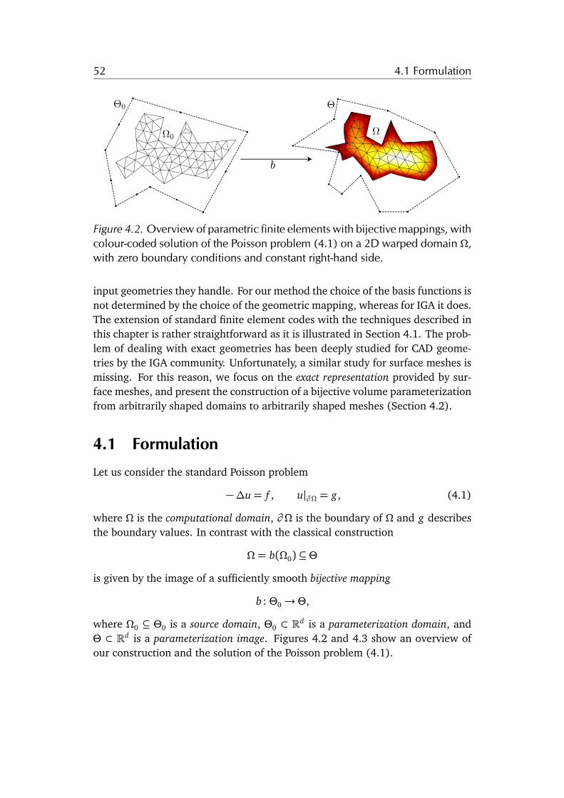
52 4.1 Formulation
b
Figure 4.2. Overview of parametric finite elements with bijective mappings, withcolour-coded solution of the Poisson problem (4.1) on a 2D warped domain ⌦,with zero boundary conditions and constant right-hand side.
input geometries they handle. For our method the choice of the basis functions isnot determined by the choice of the geometric mapping, whereas for IGA it does.The extension of standard finite element codes with the techniques described inthis chapter is rather straightforward as it is illustrated in Section 4.1. The prob-lem of dealing with exact geometries has been deeply studied for CAD geome-tries by the IGA community. Unfortunately, a similar study for surface meshes ismissing. For this reason, we focus on the exact representation provided by sur-face meshes, and present the construction of a bijective volume parameterizationfrom arbitrarily shaped domains to arbitrarily shaped meshes (Section 4.2).
4.1 Formulation
Let us consider the standard Poisson problem
��u= f , u|@⌦ = g, (4.1)
where ⌦ is the computational domain, @⌦ is the boundary of ⌦ and g describesthe boundary values. In contrast with the classical construction
⌦ = b(⌦0) ✓ ⇥is given by the image of a sufficiently smooth bijective mapping
b : ⇥0! ⇥,
where ⌦0 ✓ ⇥0 is a source domain, ⇥0 ⇢ Rd is a parameterization domain, and⇥ ⇢ Rd is a parameterization image. Figures 4.2 and 4.3 show an overview ofour construction and the solution of the Poisson problem (4.1).
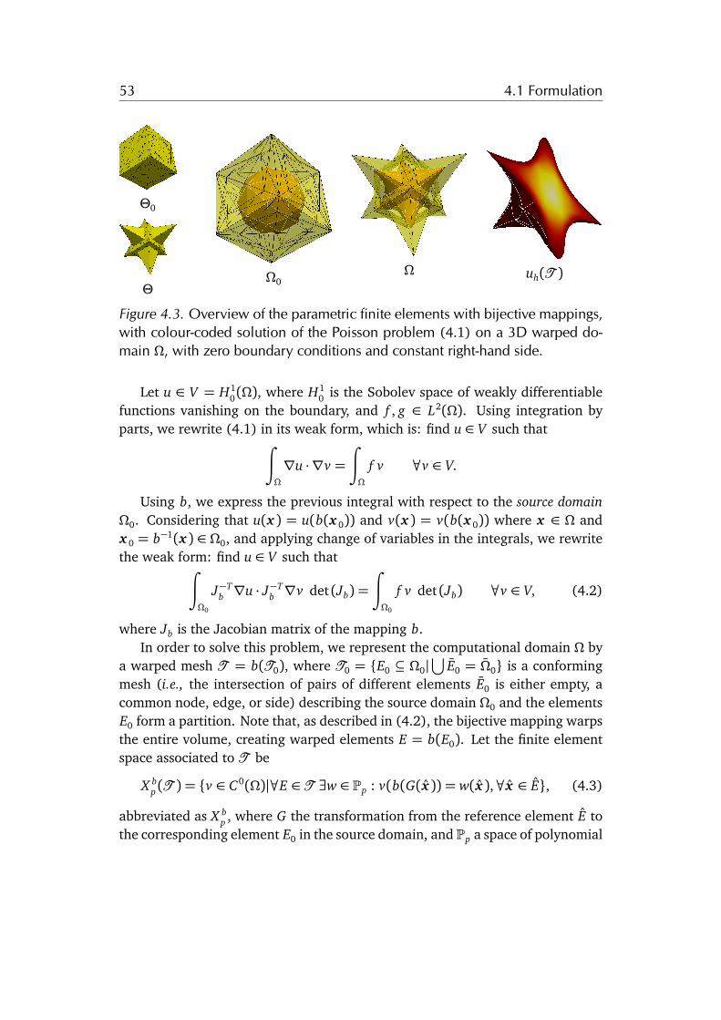
53 4.1 Formulation
⇥0
⇥⌦0
⌦ uh(T )
Figure 4.3. Overview of the parametric finite elements with bijective mappings,with colour-coded solution of the Poisson problem (4.1) on a 3D warped do-main ⌦, with zero boundary conditions and constant right-hand side.
Let u 2 V = H10(⌦), where H1
0 is the Sobolev space of weakly differentiablefunctions vanishing on the boundary, and f , g 2 L2(⌦). Using integration byparts, we rewrite (4.1) in its weak form, which is: find u 2 V such that
Z
⌦
ru ·rv =Z
⌦
f v 8v 2 V.
Using b, we express the previous integral with respect to the source domain⌦0. Considering that u(x ) = u(b(x 0)) and v(x ) = v(b(x 0)) where x 2 ⌦ andx 0 = b�1(x ) 2 ⌦0, and applying change of variables in the integrals, we rewritethe weak form: find u 2 V such that
Z
⌦0
J�Tb ru · J�T
b rv det (Jb) =Z
⌦0
f v det (Jb) 8v 2 V, (4.2)
where Jb is the Jacobian matrix of the mapping b.In order to solve this problem, we represent the computational domain ⌦ by
a warped mesh T = b(T0), where T0 = {E0 ✓ ⌦0|S E0 = ⌦0} is a conformingmesh (i.e., the intersection of pairs of different elements E0 is either empty, acommon node, edge, or side) describing the source domain ⌦0 and the elementsE0 form a partition. Note that, as described in (4.2), the bijective mapping warpsthe entire volume, creating warped elements E = b(E0). Let the finite elementspace associated to T be
X bp (T ) = {v 2 C0(⌦)|8E 2 T 9w 2 Pp : v(b(G(x )) = w(x ),8x 2 E}, (4.3)
abbreviated as X bp , where G the transformation from the reference element E to
the corresponding element E0 in the source domain, and Pp a space of polynomial
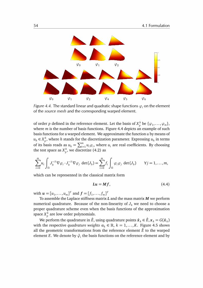
54 4.1 Formulation
'0 '1 '2
'0 '1 '2 '4 '5 '6
0
0.25
0.5
0.75
1
Figure 4.4. The standard linear and quadratic shape functions 'i on the elementof the source mesh and the corresponding warped element.
of order p defined in the reference element. Let the basis of X bp be {'1, . . . ,'m},
where m is the number of basis functions. Figure 4.4 depicts an example of suchbasis functions for a warped element. We approximate the function u by means ofuh 2 X b
p , where h stands for the discretization parameter. Expressing uh in termsof its basis reads as uh =
Pmi=1 ui'i, where ui are real coefficients. By choosing
the test space as X bp , we discretize (4.2) as
mX
i=0
ui
Z
⌦
J�Tb r'i · J�T
b r' j det (Jb) =mX
i=0
fi
Z
⌦
'i' j det (Jb) 8 j = 1, . . . , m,
which can be represented in the classical matrix form
Lu = M f , (4.4)
with u = [u1, . . . , um]T and f = [ f1, . . . , fm]T
To assemble the Laplace stiffness matrix L and the mass matrix M we performnumerical quadrature. Because of the non-linearity of Jb we need to choose aproper quadrature scheme even when the basis functions of the approximationspace X b
p are low order polynomials.We perform the quadrature in E, using quadrature points x k 2 E, x k = G(x k)
with the respective quadrature weights ↵k 2 R, k = 1, . . . , K . Figure 4.5 showsall the geometric transformations from the reference element E to the warpedelement E. We denote by 'i the basis functions on the reference element and by
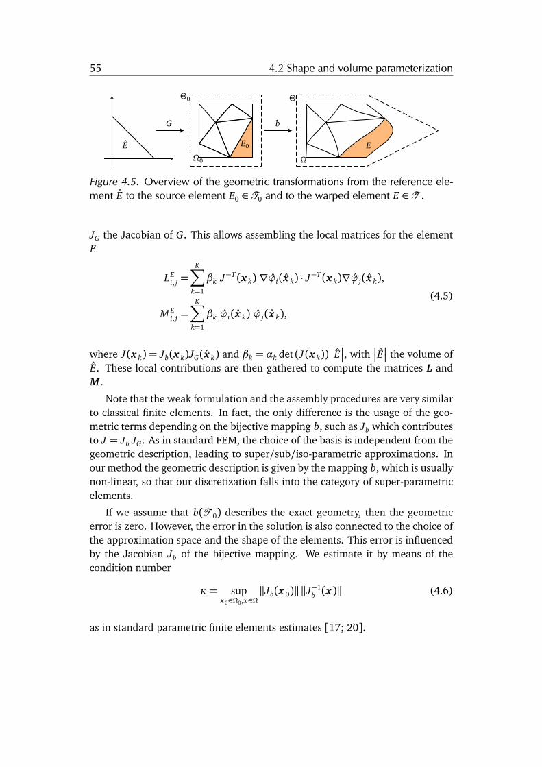
55 4.2 Shape and volume parameterization
E E0 E
G b
⇥0 ⇥
⌦0 ⌦
Figure 4.5. Overview of the geometric transformations from the reference ele-ment E to the source element E0 2 T0 and to the warped element E 2 T .
JG the Jacobian of G. This allows assembling the local matrices for the elementE
LEi, j =
KX
k=1
�k J�T (x k) r'i(x k) · J�T (x k)r' j(x k),
M Ei, j =
KX
k=1
�k 'i(x k) ' j(x k),
(4.5)
where J(x k) = Jb(x k)JG(x k) and �k = ↵k det (J(x k))��E��, with
��E�� the volume of
E. These local contributions are then gathered to compute the matrices L andM .
Note that the weak formulation and the assembly procedures are very similarto classical finite elements. In fact, the only difference is the usage of the geo-metric terms depending on the bijective mapping b, such as Jb which contributesto J = Jb JG. As in standard FEM, the choice of the basis is independent from thegeometric description, leading to super/sub/iso-parametric approximations. Inour method the geometric description is given by the mapping b, which is usuallynon-linear, so that our discretization falls into the category of super-parametricelements.
If we assume that b(T 0) describes the exact geometry, then the geometricerror is zero. However, the error in the solution is also connected to the choice ofthe approximation space and the shape of the elements. This error is influencedby the Jacobian Jb of the bijective mapping. We estimate it by means of thecondition number
= supx 02⌦0,x2⌦
kJb(x 0)kkJ�1b (x )k (4.6)
as in standard parametric finite elements estimates [17; 20].
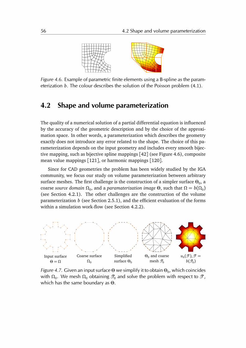
56 4.2 Shape and volume parameterization
Figure 4.6. Example of parametric finite elements using a B-spline as the param-eterization b. The colour describes the solution of the Poisson problem (4.1).
4.2 Shape and volume parameterization
The quality of a numerical solution of a partial differential equation is influencedby the accuracy of the geometric description and by the choice of the approxi-mation space. In other words, a parameterization which describes the geometryexactly does not introduce any error related to the shape. The choice of this pa-rameterization depends on the input geometry and includes every smooth bijec-tive mapping, such as bijective spline mappings [42] (see Figure 4.6), compositemean value mappings [121], or harmonic mappings [120].
Since for CAD geometries the problem has been widely studied by the IGAcommunity, we focus our study on volume parameterization between arbitrarysurface meshes. The first challenge is the construction of a simpler surface ⇥0, acoarse source domain ⌦0, and a paramaterization image ⇥, such that ⌦ = b(⌦0)(see Section 4.2.1). The other challenges are the construction of the volumeparameterization b (see Section 2.5.1), and the efficient evaluation of the formswithin a simulation work-flow (see Section 4.2.2).
Input surface⇥ = ⌦
Coarse surface⌦0
Simplifiedsurface ⇥0
⇥0 and coarsemesh T0
uh(T ),T =b(T0)
Figure 4.7. Given an input surface⇥we simplify it to obtain⇥0, which coincideswith ⌦0. We mesh ⌦0 obtaining T0 and solve the problem with respect to T ,which has the same boundary as ⇥.
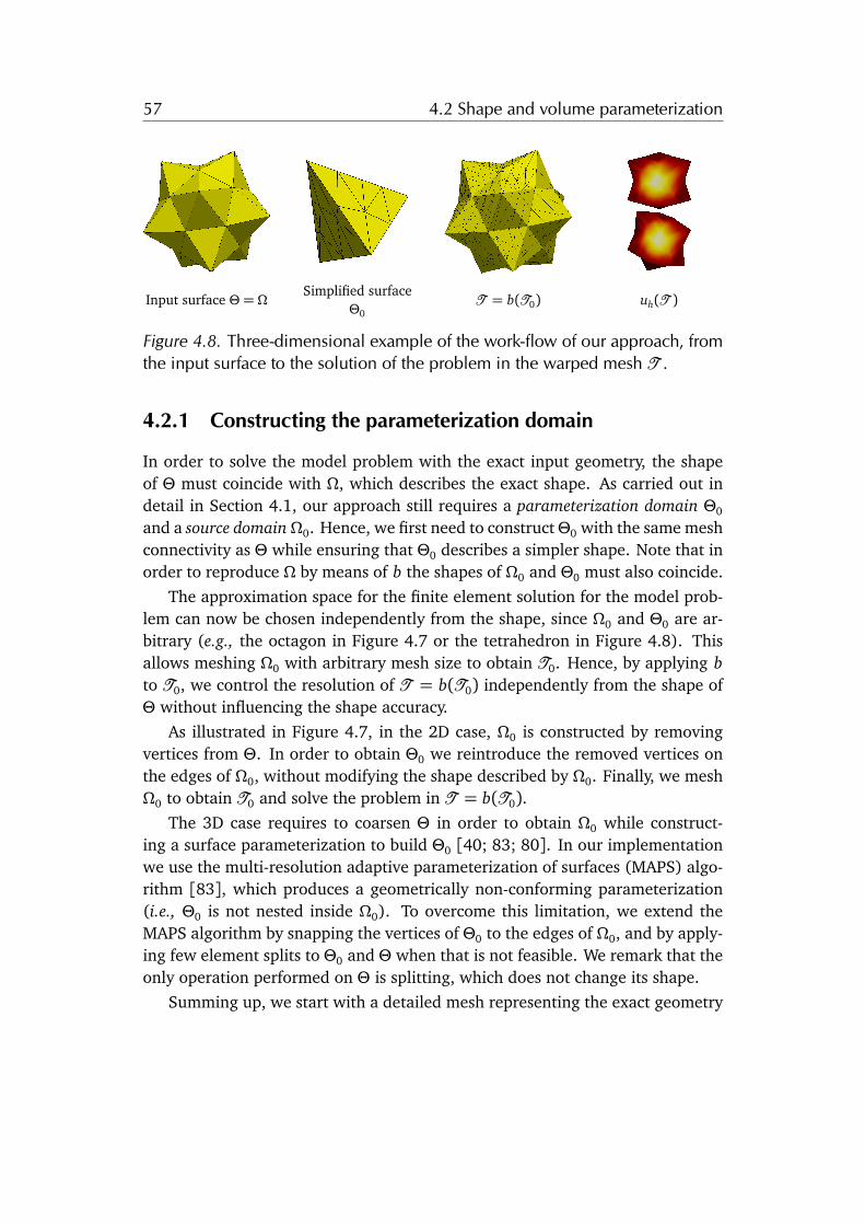
57 4.2 Shape and volume parameterization
Input surface ⇥ = ⌦Simplified surface
⇥0T = b(T0) uh(T )
Figure 4.8. Three-dimensional example of the work-flow of our approach, fromthe input surface to the solution of the problem in the warped mesh T .
4.2.1 Constructing the parameterization domain
In order to solve the model problem with the exact input geometry, the shapeof ⇥ must coincide with ⌦, which describes the exact shape. As carried out indetail in Section 4.1, our approach still requires a parameterization domain ⇥0
and a source domain⌦0. Hence, we first need to construct⇥0 with the same meshconnectivity as ⇥ while ensuring that ⇥0 describes a simpler shape. Note that inorder to reproduce ⌦ by means of b the shapes of ⌦0 and ⇥0 must also coincide.
The approximation space for the finite element solution for the model prob-lem can now be chosen independently from the shape, since ⌦0 and ⇥0 are ar-bitrary (e.g., the octagon in Figure 4.7 or the tetrahedron in Figure 4.8). Thisallows meshing ⌦0 with arbitrary mesh size to obtain T0. Hence, by applying bto T0, we control the resolution of T = b(T0) independently from the shape of⇥ without influencing the shape accuracy.
As illustrated in Figure 4.7, in the 2D case, ⌦0 is constructed by removingvertices from ⇥. In order to obtain ⇥0 we reintroduce the removed vertices onthe edges of ⌦0, without modifying the shape described by ⌦0. Finally, we mesh⌦0 to obtain T0 and solve the problem in T = b(T0).
The 3D case requires to coarsen ⇥ in order to obtain ⌦0 while construct-ing a surface parameterization to build ⇥0 [40; 83; 80]. In our implementationwe use the multi-resolution adaptive parameterization of surfaces (MAPS) algo-rithm [83], which produces a geometrically non-conforming parameterization(i.e., ⇥0 is not nested inside ⌦0). To overcome this limitation, we extend theMAPS algorithm by snapping the vertices of ⇥0 to the edges of ⌦0, and by apply-ing few element splits to ⇥0 and ⇥ when that is not feasible. We remark that theonly operation performed on ⇥ is splitting, which does not change its shape.
Summing up, we start with a detailed mesh representing the exact geometry
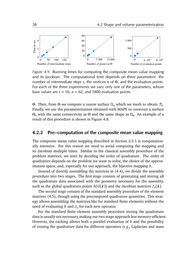
58 4.2 Shape and volume parameterization
0
50
100
150
0
2
4
Number of intermediate steps
Tim
ein
sec
0
7,500 15,000
0
20
40
60
80
Number of points in Q0
4 ·10
6
8 ·10
6
0
500
1,000
Number of evaluation points
Figure 4.9. Running times for computing the composite mean value mappingand its Jacobian. The computational time depends on three parameters: thenumber of intermediate steps s, the vertices n of ⇥, and the evaluation points.For each of the three experiments we vary only one of the parameters, whosebase values are s = 10, n= 62, and 1800 evaluation points.
⇥. Then, from ⇥ we compute a coarse surface ⌦0 which we mesh to obtain T0.Finally, we use the parameterization obtained with MAPS to construct a surface⇥0 with the same connectivity as ⇥ and the same shape as ⌦0. An example of aresult of this procedure is shown in Figure 4.8.
4.2.2 Pre–computation of the composite mean value mapping
The composite mean value mapping described in Section 2.5.1 is computation-ally intensive. For this reason we need to avoid computing the mapping andits Jacobian multiple times. Similar to the classical assembly procedure of theproblem matrices, we start by deciding the order of quadrature. The order ofquadrature depends on the problem we want to solve, the choice of the approx-imation space, and, especially for our approach, the bijective mapping b.
Instead of directly assembling the matrices in (4.4), we divide the assemblyprocedure into two stages. The first stage consists of generating and storing allthe quadrature data associated with the geometry necessary for the assembly,such as the global quadrature points b(G(x )) and the Jacobian matrices Jb(x ).
The second stage consists of the standard assembly procedure of the elementmatrices (4.5), though using the precomputed quadrature quantities. This strat-egy allows assembling the matrices like for standard finite elements without theneed of evaluating b and Jb for each new operator.
For the standard finite element assembly procedure storing the quadraturedata is usually not necessary, making our two stage approach less memory-efficient.However, the caching allows both a parallel evaluation of b and the possibilityof reusing the quadrature data for different operators (e.g., Laplacian and mass

59 4.3 Piecewise mapping approximations
Linear Quadratic Quartic
E0 b1(E0) E0 b2(E0) E0 b4(E0)
Figure 4.10. Comparison of b (orange dashed line) with its polynomial approx-imations bk (black solid line) for an element E0.
matrix) and multiple time-steps (e.g., in case of transient non-linear elasticitysimulations). For instance, in Figure 4.1 the quantities related to b are computedonly at the first time-step and reused in the following ones.
Despite the pre-computation, the evaluation of b remains expensive. For-tunately, mean value coordinates are straightforward to parallelize on sharedmemory processors. In fact, every point-wise evaluation of b and Jb can be com-puted in a completely independent way. Figure 4.9 shows the parallel-runningtimes using OpenCL [74] with respect to different input sizes, computed on alaptop computer with Intel Core i7 2.3GHz processor and 16GB RAM.
4.3 Piecewise mapping approximations
As previously mentioned, composite mean-value mappings are computationallyvery expensive and their inverse is computed by solving an even more expen-sive optimization problem. An alternative option is approximating such map-pings element-wise by a simpler geometric map. In this section we show possi-ble choices of such approximation, ranging from polynomials (Section 4.3.1) topolygonal approximations (Section 4.3.2 and Section 4.3).
4.3.1 Polynomial elements
A natural choice of a piecewise approximation of b is polynomial mappings [43].For each element E0 of the source domain mesh T0 we consider the approximategeometric map
bk(x ) =mX
j=1
cj' j(x ), (4.7)
where m is the number of interpolation nodes, ' j is a polynomial of degree atmost k, cj is the associated coefficient, and x 2 E0. The most basic procedure to
60 4.3 Piecewise mapping approximations
determine the coefficients cj is to solve the following interpolation system [132]
2664
'1(x 1), '2(x 1), . . . , 'm(x 1)'1(x 2), '2(x 2), . . . , 'm(x 2)
......
...'1(x m), '2(x m), . . . , 'm(x m)
3775
2664
c1
c2...
cm
3775 =
2664
b(x 1)b(x 2)
...b(x m)
3775 .
Figure 4.10 shows different variants of bk for k = 1,2, 4. Let
X kp(T ) := {v 2 C0(⌦)|8E 2 T 9w 2 Pp : v(x ) = w((bkG)�1(x )),8x 2 E} (4.8)
be the finite element space associated with bk, where Pp is the the space of poly-nomials of degree p in the reference element E. When p = k we are consideringthe case of iso-parametric finite elements, when p < k we are considering super-parametric finite elements, and p > k we are considering the sub-parametriccase.
The main advantage of this approach is that, once the approximation bk isconstructed, the original map b is not necessary anymore. In other words, thecomputation of b and its approximation procedure can be considered as prepro-cessing, which does not directly affect the performance of the solution process.Moreover, since bk is a polynomial, the numerical quadrature can be performedefficiently with floating point precision [127]. However, bk does not guaranteebijectivity. In fact, in the presence of large deformations or concavities this ap-proach is very likely to fail. This issue is not resolved by naively refining the meshas shown in Figure 4.13, but, in some cases, it can be alleviated by a suitable po-sitioning of the interpolation points. In this thesis we do not address such issuesand we consider exclusively standard node placements.
4.3.2 Polygonal elements
The main issue of the local polynomial approximant bk is caused by the lim-ited (or absence of) control of the accuracy of the shape of the elements in theco-domain mesh T . In other words, the shape of the element bk(E0) solely de-pends on the choice of the interpolation points, which may result in the loss ofbijectivity, as depicted in Figure 4.13.
An alternative method which reliably preserves bijectivity consists of approx-imating b(E0) by a polygon (or polyhedron in 3D) which resolution is controlledin the co-domain with arbitrary accuracy, see Figure 4.11 left. For obtainingsuch polygon, we first sample every side of E0 with n uniformly sampled points
61 4.3 Piecewise mapping approximations
x i, i = 1, . . . , n. Then, we compute b(x i) which gives us a densely sampledpolygonal approximation of b(E0). Finally, for efficiency reasons, we discardall approximately collinear points thus creating polygons with fewer vertices. Apoint x i is discarded if uT v/(kukkvk)> (1�") is true, where u= b(x i)�b(x i�1),v = b(x i+1)� b(x i), and " 2 R>0 determines the accuracy of the approximation.Since the original mapping b is rather local, our strategy naturally generatestriangles away from the boundary, as shown in Figure 4.12. This brute force ap-proach for approximating b can be replaced by adaptive discretization strategieswith the primary objectives set to preserving bijectivity and the boundary shape.In this case adaptivity may substantially improve performance of the preprocess-ing phase and reduce the minimal number of degrees of freedom imposed to thesolution process.
Standard finite element basis functions (e.g., P1 and P2) are not suitable sincethe shape of the polygon is arbitrary. For this reason we follow the approachin [128] and employ mean-value basis functions (MV), which are well definedfor any polygon. Note that mean-value coordinates for triangles coincide with theP1 basis functions as for any other barycentric coordinate. When using such basisthe assembly procedure is not performed in the reference element but directly inthe physical element E 2 T . We describe this polygonal finite element space as
XMV(T ) := {v 2 C0(⌦)|8E 2 T 9w 2MV(E) : v(x ) = w(x ),8x 2 E}, (4.9)
whereMV(E) are the mean value coordinates defined in the polygonal elementE. Note that for this discretization we do not have an explicit geometric relation-ship (i.e., volumetric map) between elements of T0 and the elements of T exceptfor a node-wise correspondence on the boundary of each element. The main ad-vantage of this discretization is that it avoids incurring in flipped triangles dueto linear edges or self intersecting elements due to polynomial oscillations. Notethat this discretization generally induces a higher number of degrees of freedomwhich are automatically determined in the proximity of the boundary.
4.3.3 Piecewise affine elements
A practical choice of geometric map between the polygonal approximations of el-ement E0 2 T0 and element E 2 T (introduced in Section 4.3.2) is the piecewiseaffine map bA. We construct bA by a means of suitable local triangulation whichis valid for both polygonal elements E0 and E. Validity of such map is ensuredif the triangulation does not create degeneracies, such as flipped or zero areaelements, in neither the polygonal approximations of E0 nor E.

62 4.3 Piecewise mapping approximations
Polygonal Piecewise-affine
E0 E E0 bA(E0)
Figure 4.11. Comparison of b (orange dashed line) with its polygonal andpiecewise-affine approximations (black solid line) for an element E0.
The geometric map bA can be employed with different choices of finite ele-ment functions in the reference element, such as P1 and P2. We denote this finiteelement space as
X Ap(T ) := {v 2 C0(⌦)|8E 2 T 9w 2 Pp : v(x ) = w((bAG)�1(x )),8x 2 E},
(4.10)where bA is defined piecewise within each element as an affine transformationwhich maps each simplex S0
k ✓ E0 2 T0 to their image Sk ✓ E 2 T . An exampleof element bA(E0) is depicted in Figure 4.11 right.
Figure 4.12. Number of nodes per element. The color represents the numberof vertices of the polygonal elements, where white describes triangles and redmore complex polygons.

63 4.3 Piecewise mapping approximations
Sour
cedo
mai
nm
eshT 0
War
ped
dom
ain
mes
hT=
b(T 0)
Line
arap
prox
imat
ion
Qua
drat
icap
prox
imat
ion
Qua
rtic
appr
oxim
atio
nPo
lygo
nalo
rpi
ecew
ise
affin
eap
prox
imat
ion
Original mesh One refinement Two refinements
Figure 4.13. Comparison between b and its different element-wise approxima-tions. The loss of bijectivity for linear, quadratic and quartic approximationsaround concavities is not mitigated by refinement. Note that refining the meshmay actually introduce this problem, as visible in the second column of thequartic approximation.
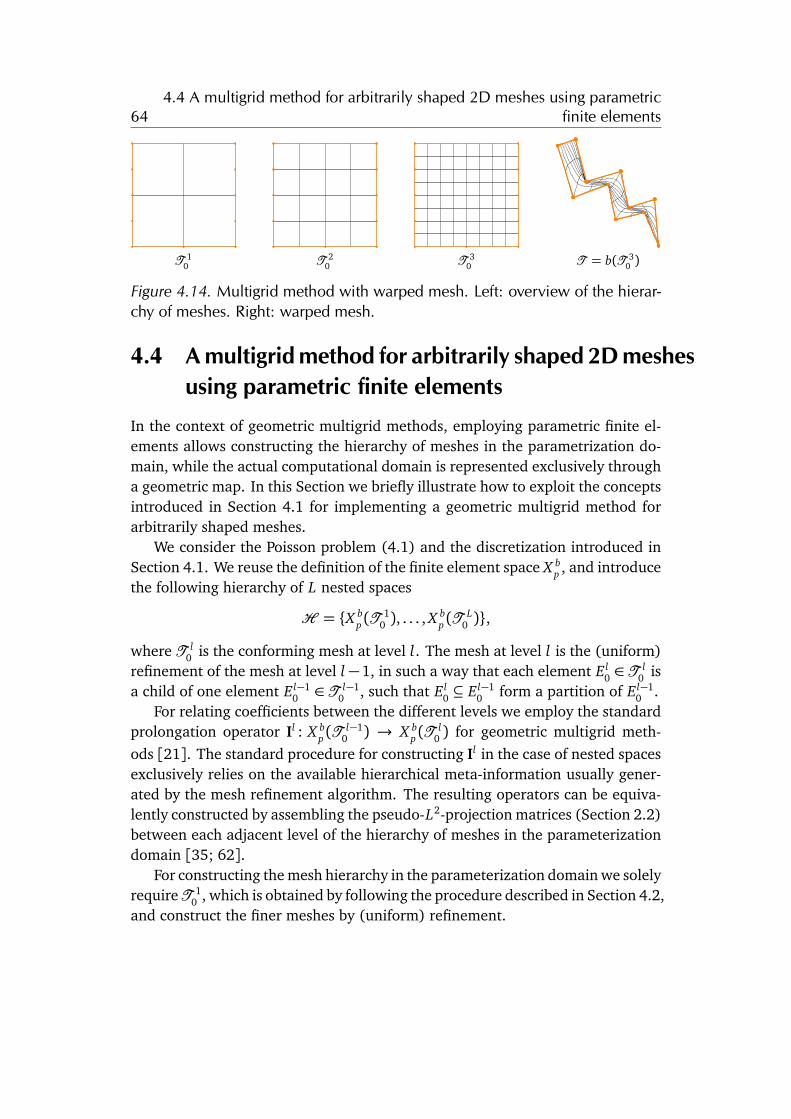
644.4 A multigrid method for arbitrarily shaped 2D meshes using parametric
finite elements
T 10 T 2
0 T 30 T = b(T 3
0 )
Figure 4.14. Multigrid method with warped mesh. Left: overview of the hierar-chy of meshes. Right: warped mesh.
4.4 A multigrid method for arbitrarily shaped 2D meshesusing parametric finite elements
In the context of geometric multigrid methods, employing parametric finite el-ements allows constructing the hierarchy of meshes in the parametrization do-main, while the actual computational domain is represented exclusively througha geometric map. In this Section we briefly illustrate how to exploit the conceptsintroduced in Section 4.1 for implementing a geometric multigrid method forarbitrarily shaped meshes.
We consider the Poisson problem (4.1) and the discretization introduced inSection 4.1. We reuse the definition of the finite element space X b
p , and introducethe following hierarchy of L nested spaces
H = {X bp (T 1
0 ), . . . , X bp (T L
0 )},where T l
0 is the conforming mesh at level l. The mesh at level l is the (uniform)refinement of the mesh at level l �1, in such a way that each element El
0 2 T l0 is
a child of one element El�10 2 T l�1
0 , such that El0 ✓ El�1
0 form a partition of El�10 .
For relating coefficients between the different levels we employ the standardprolongation operator Il : X b
p (T l�10 ) ! X b
p (T l0 ) for geometric multigrid meth-
ods [21]. The standard procedure for constructing Il in the case of nested spacesexclusively relies on the available hierarchical meta-information usually gener-ated by the mesh refinement algorithm. The resulting operators can be equiva-lently constructed by assembling the pseudo-L2-projection matrices (Section 2.2)between each adjacent level of the hierarchy of meshes in the parameterizationdomain [35; 62].
For constructing the mesh hierarchy in the parameterization domain we solelyrequireT 1
0 , which is obtained by following the procedure described in Section 4.2,and construct the finer meshes by (uniform) refinement.

65 4.5 Chapter conclusion
Once our hierarchy is constructed, we assemble the matrix L and related ma-trices and vectors from (4.4) on level L. We construct the stiffness matrices in thecoarse levels by performing the Galerkin projections Ll�1 = (Il)T LlIl . In a similarfashion, within the multigrid algorithm, we restrict the residual as rl�1 = (Il)T rl ,where rL =Mf� Lu and interpolate the correction as cl = Ilcl�1.
Instead of employing the map b we can exploit its piecewise approximationsfor a more efficient finite element assembly. In the case of the piecewise polyno-mial approximation of b introduced in Section 4.3 we can just swap b with bk inthe definitions of the multigrid hierarchy. With the finite element space X k
p(T l)from (4.7), where Tl = (bk(T l
0 )), we describe the finite element space associatedwith level l = 1, . . . , L of the multigrid hierarchy
H kp = {X k
p(T 1), . . . , X kp(T L)}.
For the polygonal finite element approximation we have no explicit map ap-proximation that we can employ. Hence, we define the coarse space X Q
MV(T l) =spank2Jl
{ k} on the l level, where Jl ⇢ N is the index set of the nodes of T l .Let us introduce the weight matrix Q 2 R|Jl+1|⇥|Jl | with elements qi j,
Pj2Jl
qi j = 1,and follows the definition i =
Pj2Jl
qi j✓ j, with X QMV(T l+1) = spank2Jl+1
{✓k}.The weight matrix is constructed by assemblying the L2-projection operator be-tween the auxiliary spaces XMV(T l
0 ), which are defined in the parameterizationdomain, as described in Section 2.2. Note that, in our set-up, for l < L we haveXMV(T l
0 ) = X 11(T l
0 ). The recursive definition of X QMV(T l) at its base case is de-
fined as X QMV(T L) := XMV(T ), which allows us to express this multigrid hierarchy
asHMV = {X Q
MV(T 1), . . . , X QMV(T L)}.
4.5 Chapter conclusion
The idea of combining the finite element method with bijective mappings allowsrepresenting complex geometries on coarse meshes and enables specifying inter-polation conditions as in the classical finite element method. For instance, ourmethod can be used with Lagrange elements, splines, NURBS, or mixed finite el-ements independently from the complexity of the input geometry. We introducethis novel discretization focusing on the particular case of composite mean valuemappings which automatically creates a volume parameterization given only theboundary description.
Although we focus our presentation on the case of discrete geometry and com-posite mean value mappings, our construction might be suitable for any other

66 4.5 Chapter conclusion
Figure 4.15. Handling the interface (grey stars) between the Neumann boundary(blue solid lines) and the the Dirichlet boundary (orange dashed lines) from ⇥to T0.
choice of bijective mapping b, and it would be interesting to further investigatethis flexibility. For instance, within the composite mapping, we can employ othertypes of smooth barycentric coordinates for which we can compute the Jacobian,such as maximum entropy coordinates [66; 52]. The method becomes compu-tationally more expensive when employing the composite mean value mapping,however much of the related data can be precomputed and reused for differ-ent operators, as explained in Section 4.2.2. Moreover from the assembly pointof view, our method only requires to change to quadrature procedure (4.5) byincluding the terms containing b.
In our presentation we first defined the mapping b as a global parameteriza-tion from⇥0 to⇥, though, in order to have a faster computation of the quadraturedata, we discussed strategies for localizing the mapping.
We presented the integration of our approach with efficient and modern solu-tion techniques, such as multigrid methods. The flexibility provided by arbitrarilychoosing the mesh for describing ⌦0, allows us to naturally generate nested geo-metric multigrid hierarchies with exact geometry. Moreover, the construction ofthe interpolation and restriction operators is trivially performed using standardmesh refinement of the source mesh T0, since the mapping b is the same for alllevels.
Our discretization with composite mean value mapping enables treating bound-ary conditions with arbitrary precision even for the non-homogeneous case. Forinstance, let us consider the example problem in Figure 4.15, where Dirichletboundary conditions are specified on @⌦D ✓ @⌦ (orange dashed lines) and Neu-mann conditions on @⌦N = @⌦ \ @⌦D (blue solid lines). Let the interface (greystars) between @⌦D and @⌦N be � and its corresponding interface in⇥0 be �0 (i.e.,� = b(�0)). When generating the mesh T0 we preserve �0 which is then mappedto its image � in T . Since � is preserved, the boundary conditions which arespecified on @⌦D and @⌦N can be equivalently handled on ⌦0.
67 4.5 Chapter conclusion
A limitation which comes with our choice of bijective mapping b is that com-posite mean-value mappings do not provide any guarantees nor control over thequality of the computational mesh, which is usually determined by aspect-ratioand orientation of the elements [125]. In fact, the shape of the elements is en-tirely subject to any distortion caused by the mapping b. This suggests that fur-ther investigations on this topic are necessary for providing mesh-quality guaran-tees that are conforming to industry standards or enabling synergies with state-of-the-art methods, such as r-refinement [98]. In Section 4.3 we presented theelement-wise approximations of b which may present future opportunities forlocalized mesh improvement and mesh adaption.

68 4.5 Chapter conclusion
Chapter 5
Utopia: a C++ embedded domainspecific language for scientificcomputing
In this chapter we present UTOPIA which is an eDSL deeply embedded in C++.Its philosophy is the separation of model and computation and its main purposesare linear and non-linear algebra, and finite element simulations. By exploit-ing meta-programming facilities, UTOPIA can easily be integrated with any otherexisting implementation, hence it is independent from technological changes.Moreover, UTOPIA shares the advantages of DSLs, for instance hidden paral-lelism, optimization transparency, and automatic differentiation. The UTOPIA
eDSL is designed and developed for providing a balance between abstractionand low-level access without sacrificing performance. It aims at an organic in-tegration with existing code without creating barriers between abstractions andimplementation. In fact, both abstractions and low-level data are accessible tothe user at any time. This allows users to extend their code with possibly missingfunctionalities by manipulating the low-level data (and back-end) directly. Theflexible design of UTOPIA allows for adding these features in a straightforwardway to future releases.
UTOPIA follows object oriented programming (OOP) principles [92]. An ex-ample is design-by-contract [96]which states that interfaces specified in the super-type have to be respected in the sub-type. A violation of the contract leads tocode that, even if it compiles, does not run correctly. This type of fragility iscommon, and a way of handling this issue consists of hiding as many details aspossible behind high-level abstractions. The UTOPIA abstraction performs all nec-essary work-around to ensure that the client code, when compiles and respects
69
70 5.1 Architecture
the contract (which is automatically checked with assertions) runs without fail-ures. Another important OOP principle is the dependency inversion principle [92]which states that high-level abstractions should dictate how high- and low-levelmodules have to be integrated. The implementation of UTOPIA is built and de-veloped on top of this principle. Finally, other important OOP principles, such asthe open/close principle, are taken into consideration when developing UTOPIA.The respect of these principles, allows UTOPIA to be modular, reusable, easy toextend, and sustainable to maintain.
This chapter is organized as follows: in Section 5.1 we explain the princi-ples and design of UTOPIA, in Section 5.2 we present some extensions, and inSection 5.3 we provide a set of scenarios to show the usage of UTOPIA in anapplication environment.
5.1 Architecture
Many powerful linear algebra libraries (e.g., PETSc, UBLAS [134], and AR-MADILLO [119]) or finite element libraries (e.g., LIBMESH, MFEM [77], DUNE [9],and FETK [65]) already exist. For this reason, the first prototype of UTOPIA doesnot “reinvent the wheel” and relies on PETSc for the algebra and LIBMESH forthe finite element assembly. It is possible to develop other back-ends, such asautomatic OPENCL code generators.
The design of the UTOPIA core is based on three main components: theeDSL (Section 5.1.1), the expression-tree (Section 5.1.2), and the evaluator (Sec-tion 5.1.3), which are represented in the component diagram in Figure 5.1. TheUTOPIA eDSL allows users to state the behavior of their program and only careabout the details relevant to their application. Despite this high degree of ab-straction, users may need to perform operations on concrete data-types, such asaccessing the entries of a matrix. To facilitate such tasks, UTOPIA provides anapplication programming interface (API) which directly queries the back-end forparticular data (Section 5.1.4).
Natively, UTOPIA does not compute any of the specified operations since itrelies solely on its back-ends. We use expression-trees to evaluate the operationsdepending either on the overall evaluation strategy or the specific back-end prop-erties. We note that evaluation and back-end are conceptually tightly coupled.For instance, if the back-end is a library such as PETSc, we tailor the evaluationof the expression tree to the specific C functions.

71 5.1 Architecture
expression tree
evaluator
expression to function mapping
code generation
back-end
BLASPETSc
LAPACK ...
eDSL
element-wise evaluation
API
Figure 5.1. Component diagram of the UTOPIA core, the main components arehighlighted. The connectors describe the dependency relationships among com-ponents, where the circle represents an interface and the arc represents the us-age of such interface.
5.1.1 Embedded domain specific language
The UTOPIA eDSL primitives are mainly inspired by MATLAB and EIGEN [55], andare realized by exploiting the C++ language meta-programming facilities (i.e.,templates), function overloading, and functional-style programming constructsintroduced in the C++11 standard. The simple and clean presentation to usersis made possible by type inference and the auto keyword which allows to hidecomplex meta types, see Figure 5.2.
Tensor types are represented by the wrapper class template<class Tensor,int Order> class Wrapper within UTOPIA expression-trees. The first templateparameter Tensor is the concrete back-end type, for instance a PETSc matrix.The second parameter Order is the tensorial order, for instance Wrapper<Tensor,1> describes vectors and Wrapper<Tensor, 2> describes matrices. Interactionbetween wrappers is defined through the UTOPIA primitives, for instance themultiplication or transpose operator. This interaction automatically generatesan expression tree which is evaluated only when it is assigned to another wrap-per object. Direct wrapper manipulation (e.g., changing the entries of a vector)is implemented in a unified API (Section 5.1.4).
5.1.2 Expression tree
The nodes of the tree are expressions and can be either operations, wrapper ob-jects, or factories. The actual expression tree is generated by combining multipleexpression nodes, as shown in Figure 5.3. Operations are branches of the tree
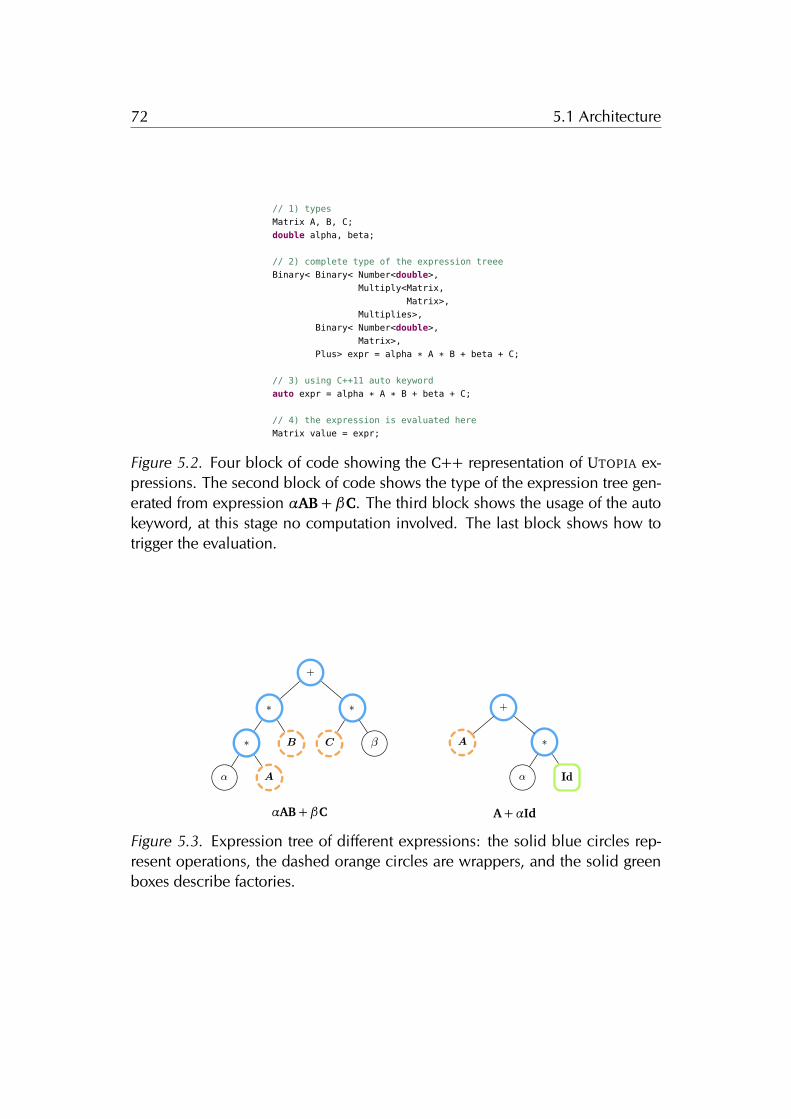
72 5.1 Architecture
// 1) typesMatrix A, B, C;double alpha, beta;
// 2) complete type of the expression treeeBinary< Binary< Number<double>,
Multiply<Matrix,Matrix>,
Multiplies>,Binary< Number<double>,
Matrix>,Plus> expr = alpha * A * B + beta + C;
// 3) using C++11 auto keywordauto expr = alpha * A * B + beta + C;
// 4) the expression is evaluated hereMatrix value = expr;
Figure 5.2. Four block of code showing the C++ representation of UTOPIA ex-pressions. The second block of code shows the type of the expression tree gen-erated from expression ↵AB+ �C. The third block shows the usage of the autokeyword, at this stage no computation involved. The last block shows how totrigger the evaluation.
+
**
B*
A®
C ¯ A
+
*
® Id
↵AB+ �C A+↵Id
Figure 5.3. Expression tree of different expressions: the solid blue circles rep-resent operations, the dashed orange circles are wrappers, and the solid greenboxes describe factories.
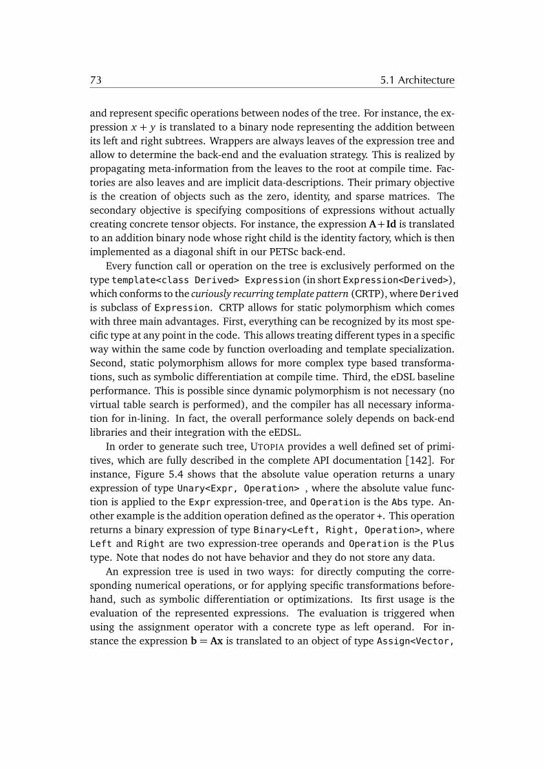
73 5.1 Architecture
and represent specific operations between nodes of the tree. For instance, the ex-pression x + y is translated to a binary node representing the addition betweenits left and right subtrees. Wrappers are always leaves of the expression tree andallow to determine the back-end and the evaluation strategy. This is realized bypropagating meta-information from the leaves to the root at compile time. Fac-tories are also leaves and are implicit data-descriptions. Their primary objectiveis the creation of objects such as the zero, identity, and sparse matrices. Thesecondary objective is specifying compositions of expressions without actuallycreating concrete tensor objects. For instance, the expression A+ Id is translatedto an addition binary node whose right child is the identity factory, which is thenimplemented as a diagonal shift in our PETSc back-end.
Every function call or operation on the tree is exclusively performed on thetype template<class Derived> Expression (in short Expression<Derived>),which conforms to the curiously recurring template pattern (CRTP), where Derivedis subclass of Expression. CRTP allows for static polymorphism which comeswith three main advantages. First, everything can be recognized by its most spe-cific type at any point in the code. This allows treating different types in a specificway within the same code by function overloading and template specialization.Second, static polymorphism allows for more complex type based transforma-tions, such as symbolic differentiation at compile time. Third, the eDSL baselineperformance. This is possible since dynamic polymorphism is not necessary (novirtual table search is performed), and the compiler has all necessary informa-tion for in-lining. In fact, the overall performance solely depends on back-endlibraries and their integration with the eEDSL.
In order to generate such tree, UTOPIA provides a well defined set of primi-tives, which are fully described in the complete API documentation [142]. Forinstance, Figure 5.4 shows that the absolute value operation returns a unaryexpression of type Unary<Expr, Operation> , where the absolute value func-tion is applied to the Expr expression-tree, and Operation is the Abs type. An-other example is the addition operation defined as the operator +. This operationreturns a binary expression of type Binary<Left, Right, Operation>, whereLeft and Right are two expression-tree operands and Operation is the Plustype. Note that nodes do not have behavior and they do not store any data.
An expression tree is used in two ways: for directly computing the corre-sponding numerical operations, or for applying specific transformations before-hand, such as symbolic differentiation or optimizations. Its first usage is theevaluation of the represented expressions. The evaluation is triggered whenusing the assignment operator with a concrete type as left operand. For in-stance the expression b = Ax is translated to an object of type Assign<Vector,
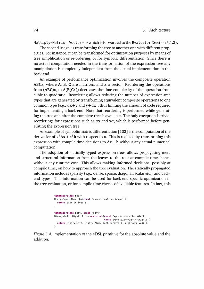
74 5.1 Architecture
Multiply<Matrix, Vector> >which is forwarded to the Evaluator (Section 5.1.3).The second usage, is transforming the tree to another one with different prop-
erties. For instance, it can be transformed for optimization purposes by means oftree simplification or re-ordering, or for symbolic differentiation. Since there isno actual computation needed in the transformation of the expression tree anymanipulation is completely independent from the actual implementation in theback-end.
An example of performance optimization involves the composite operationABCx, where A, B, C are matrices, and x a vector. Reordering the operationsfrom (ABC)x, to A(B(Cx)) decreases the time complexity of the operation fromcubic to quadratic. Reordering allows reducing the number of expression-treetypes that are generated by transforming equivalent composite operations to onecommon type (e.g., ↵x+y and y+↵x), thus limiting the amount of code requiredfor implementing a back-end. Note that reordering is performed while generat-ing the tree and after the complete tree is available. The only exception is trivialreorderings for expressions such as ↵x and x↵, which is performed before gen-erating the expression tree.
An example of symbolic matrix differentiation [103] is the computation of thederivative of xT Ax+ xT b with respect to x. This is realized by transforming thisexpression with compile time decisions to Ax+ b without any actual numericalcomputation.
The adoption of statically typed expression-trees allows propagating metaand structural information from the leaves to the root at compile time, hencewithout any runtime cost. This allows making informed decisions, possibly atcompile time, on how to approach the tree evaluation. The statically propagatedinformation includes sparsity (e.g., dense, sparse, diagonal, scalar etc.) and back-end types. This information can be used for back-end specific optimization inthe tree evaluation, or for compile time checks of available features. In fact, this
template<class Expr>Unary<Expr, Abs> abs(const Expression<Expr> &expr) {return expr.derived();
}
template<class Left, class Right>Binary<Left, Right, Plus> operator+(const Expression<Left> &left,
const Expression<Right> &right) {return Binary<Left, Right, Plus>(left.derived(), right.derived());
}
Figure 5.4. Implementation of the eDSL primitive for the absolute value and theaddition.
75 5.1 Architecture
allows writing code that, once compiled, runs without encountering unsupportedoperations, broken interfaces, or errors.
5.1.3 Evaluator
The purpose of the evaluator component is computing tensorial quantities from agiven expression tree by means of back-ends (Section 5.1.3). This is performedwith three different strategies: expression to function mapping (Section 5.1.3),where the evaluator works as a dispatcher forwarding calls directly to specificback-end functions; code generation (Section 5.1.3), where the evaluator uses theexpression-tree as a guide for generating and compiling code on the fly; element-wise evaluation (Section 5.1.3), where the evaluator evaluates the expression-tree, completely or partially, in-line [133]. The design of the evaluator providesfacilities for simple and modular extensions of the delegation of function calls, al-lowing to map composite expressions to the most specific code without changingthe interface to the user.
We note that the aforementioned strategies can form a synergy. By exploitingstatically typed expression-trees, we can match particular branches to specificstrategies. For instance, when evaluating expression templates by in-line opera-tion, the lack of specificity in the evaluation of an expression (e.g., matrix matrixmultiplication) might dramatically affect performance in a negative way (due tocache misses). However, creating many intermediate representation might beinefficient as well, since memory allocation is very costly. The combination ofdifferent strategies can overcome this problems.
Back-end
The back-end provides data-types and algorithms. Usually it is either an externallibrary, such as PETSc or UBLAS, or a composition of libraries. In order to conformto a common interface, libraries might be wrapped into an interface adapter. Theevaluator binds the eDSL abstractions to the concrete types and algorithms ofspecific libraries depending on the desired strategy. The back-end adapter is alsoused by the API functions for accessing structural information such as matrixsizes or entries.
Expression to function mapping
This strategy is performed by mapping expressions to functions of specific back-ends. This is done by matching the types of specific expression-trees (or sub-

76 5.1 Architecture
void build(int n, double val, std::vector<double> &v) {v.resize(n);std::fill(v.begin(), v.end(), val);
}
Figure 5.5. Example back-end implementation for the factory function values.
trees) by means of (partial) template specialization and delegating the computa-tion to specific functions. The functions are applied in a functional programmingstyle deemed possible by C++11 return value optimization (RVO) and move se-mantics. For instance, the factory Vector v = values(n, 0.1); in our cus-tom back-end is mapped to the function in Figure 5.5 which constructs a vectorof length n with entries equal to 0.1.
More complex composite expressions (i.e., sub-trees) are mapped to specificback-end calls; for instance the vectorial expression y= ↵x+ y is mapped to theBLAS function axpy. Another example is matricial expression C = ↵AB + �Cwhich is mapped to the function dgemm_ in BLAS for which a representation ofthe tree is depicted in Figure 5.3. Similar mappings are possible in the PETScback-end, for instance the evaluation of the a triple matrix product of the formPT AP is mapped to the PETSc function MatPtAP, as shown in Figure 5.6.
The minimal requirements for a back-end are to map basic operations, such asaddition and multiplication. The mapping of composite expressions to specificfunction calls can be gradually integrated. As a consequence, all the existingapplication codes will automatically benefit from the performance given by thespecific function without changing a line of code.
Code generation
This strategy aims to generate code in a different language such as OPENCL. Insuch a way the evaluator generates, compiles, and runs programs following ajust-in-time (JIT) approach similarly to VIENNACL. Statically typed expressionsallow automatically generating and compiling specific sub-trees only once foreach runtime. A given expression-tree is divided into several sub-trees whichrepresent the concurrent portions of the algorithm where synchronization is notrequired. For each of these sub-trees we generate and compile a computationalkernel, or retrieve an already compiled one. The implementation of this particu-lar part of UTOPIA is in a primitive stage and it only serves as a proof-of-concept.
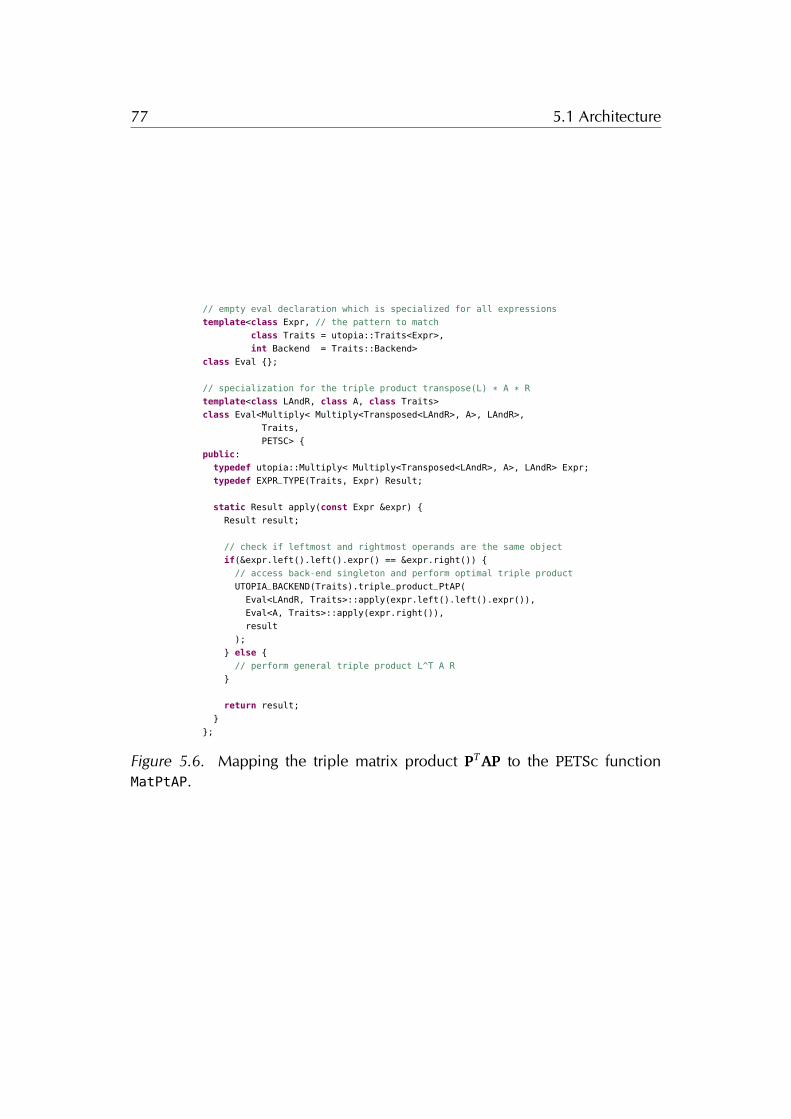
77 5.1 Architecture
// empty eval declaration which is specialized for all expressionstemplate<class Expr, // the pattern to match
class Traits = utopia::Traits<Expr>,int Backend = Traits::Backend>
class Eval {};
// specialization for the triple product transpose(L) * A * Rtemplate<class LAndR, class A, class Traits>class Eval<Multiply< Multiply<Transposed<LAndR>, A>, LAndR>,
Traits,PETSC> {
public:typedef utopia::Multiply< Multiply<Transposed<LAndR>, A>, LAndR> Expr;typedef EXPR_TYPE(Traits, Expr) Result;
static Result apply(const Expr &expr) {Result result;
// check if leftmost and rightmost operands are the same objectif(&expr.left().left().expr() == &expr.right()) {// access back-end singleton and perform optimal triple productUTOPIA_BACKEND(Traits).triple_product_PtAP(Eval<LAndR, Traits>::apply(expr.left().left().expr()),Eval<A, Traits>::apply(expr.right()),result
);} else {// perform general triple product L^T A R
}
return result;}
};
Figure 5.6. Mapping the triple matrix product PT AP to the PETSc functionMatPtAP.
78 5.1 Architecture
Element-wise evaluation
Element-wise evaluation exploits the wrapper API for evaluating an expressiontree following the typical implementation of expression-templates meta-programming.Expression templates are a well known and widely used technique for linear al-gebra libraries, such as EIGEN, and have two main advantages. First, element-wise operations can be concatenated and evaluated without creating interme-diate data. This potentially allows the compiler to “in-line” operations [69] andachieve comparable performance with respect to the most specific code for a par-ticular task. Second, it allows to write expressions using operators thus providingan aesthetic syntax similar to the classical mathematical writing.
In UTOPIA, this type of evaluation also allows for convenient interoperabil-ity between wrappers belonging to different back-ends without requiring neithercopies nor conversions. Additionally, instead of directly evaluating expressionsthrough the API, we can exploit libraries such as EIGEN as back-ends by translat-ing the UTOPIA expression-tree (Section 5.1.2) directly to back-end representa-tion.
5.1.4 API and memory access transparency
The eDSL is accompanied by a uniform API for basic interactions with tensors,such as accessors and mutators (or getters and setters). Nevertheless, back-endtypes are accessible by means of the raw_type function which takes an UTOPIA
tensor and returns its back-end representation. This allows users to directly ma-nipulate the back-end representation, for instance to add specific missing fea-tures.
Although UTOPIA provides a certain degree of transparency and strives forsimplicity, it requires that operations are handled in a “memory-conscious” man-ner, as shown in Figure 5.7. Since UTOPIA targets large scale computations andheterogeneous computing, three main aspects related to memory location needto be explicitly handled.
The first aspect concerns distributed memory access. For instance, computenodes of a supercomputer have separated dedicated memory, which implies thatthe data accessible to one node is not directly accessible to another one. In fact,independently of the particular back-end, with UTOPIA it is mandatory to useranges and their associated functions to deal with data distributions. Range ob-jects allow to iterate over elements of tensors, which are available in the localaddress space.
The second aspect regards data acquisition. For instance, a memory region on
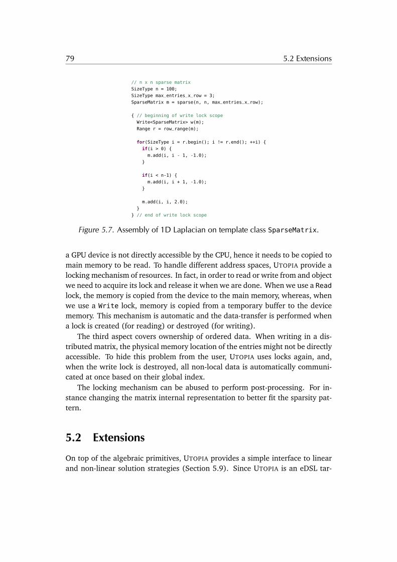
79 5.2 Extensions
// n x n sparse matrixSizeType n = 100;SizeType max_entries_x_row = 3;SparseMatrix m = sparse(n, n, max_entries_x_row);
{ // beginning of write lock scopeWrite<SparseMatrix> w(m);Range r = row_range(m);
for(SizeType i = r.begin(); i != r.end(); ++i) {if(i > 0) {m.add(i, i - 1, -1.0);
}
if(i < n-1) {m.add(i, i + 1, -1.0);
}
m.add(i, i, 2.0);}
} // end of write lock scope
Figure 5.7. Assembly of 1D Laplacian on template class SparseMatrix.
a GPU device is not directly accessible by the CPU, hence it needs to be copied tomain memory to be read. To handle different address spaces, UTOPIA provide alocking mechanism of resources. In fact, in order to read or write from and objectwe need to acquire its lock and release it when we are done. When we use a Readlock, the memory is copied from the device to the main memory, whereas, whenwe use a Write lock, memory is copied from a temporary buffer to the devicememory. This mechanism is automatic and the data-transfer is performed whena lock is created (for reading) or destroyed (for writing).
The third aspect covers ownership of ordered data. When writing in a dis-tributed matrix, the physical memory location of the entries might not be directlyaccessible. To hide this problem from the user, UTOPIA uses locks again, and,when the write lock is destroyed, all non-local data is automatically communi-cated at once based on their global index.
The locking mechanism can be abused to perform post-processing. For in-stance changing the matrix internal representation to better fit the sparsity pat-tern.
5.2 Extensions
On top of the algebraic primitives, UTOPIA provides a simple interface to linearand non-linear solution strategies (Section 5.9). Since UTOPIA is an eDSL tar-
80 5.2 Extensions
geting scientific computing it includes a prototype for finite element assembly(Section 5.2.2). Finally, for facilitating debugging activities, UTOPIA is accompa-nied by two visualization tools, one allowing to inspect algebraic data, and theother to display functions on 3D meshes (Section 5.2.3).
5.2.1 Solvers as eDSL primitives
In UTOPIA, the representations of direct and iterative solution methods are de-signed for optimization problems arising from partial differential equations. Theyconform to the same idea applied to algebraic expressions, that is the separationof model and computation. This design methodology follows two directions. Onthe one hand, we reuse as many existing implementations as possible by inter-facing with external solvers, such as PETSc’s KSP and SNES. For instance, theLUFactorization<Matrix, Vector> class uses different implementations suchas LAPACK for our custom back-end, or MUMPS [2] for PETSc. This might notapply to all solvers, since some implementations might be unavailable for a par-ticular configuration, which results in the application not compiling.
On the other hand, we develop new generic solvers on top of UTOPIA algebraicprimitives, hence they can be used with any wrapper. For instance, our imple-mentation of the trust-region algorithm is the same for our custom back-end andcode-generation back-end. The only difference is how the primitive operationsare performed.
In order to exploit a wide range of existing scientific software applicationsUTOPIA ensures interoperability with finite element libraries such as FENICS andMOOSE. The class Function (Figure 5.8) is designed to ensure this interoper-ability, by providing a uniform interface between external libraries and UTOPIA
solvers.The interface to UTOPIA solvers is designed with several levels of abstrac-
tion. Users may call the high level routine solve(). This routine does notexpose any detail and uses a default strategy to solve a system of equations.However, some problems require different solution strategies. For instance, forsymmetric-positive-definite systems we can use the conjugate-gradient method,while for non-symmetric and indefinite systems we can use the preconditioned-generalized-minimal-residual (GMRES).
The modular design of solvers allows compositions of different strategies.This enables users to combine and customize different solution strategies in orderto build an efficient solver which suits their application the best, see Example 2.

81 5.2 Extensions
template<class Matrix, class Vector>class NonlinearFunction : public Function<Matrix, Vector> {public:typedef UTOPIA_SCALAR(Matrix) Scalar;
bool value(const Vector &x, Scalar &f) const override {// evaluation routine for objective functionreturn true;
}
bool gradient(const Vector &x, Vector &g) const override {// evaluation routine for gradientreturn true;
}
bool hessian(const Vector &x, Matrix &H) const override {// evaluation routine for Hessianreturn true;
}};
NonlinearFunction<Matrix, Vector> fun;Vector x = values(2, 0);solve(fun, x);
Figure 5.8. Function used with UTOPIA non-linear solvers.
5.2.2 Finite element assembly
The set of UTOPIA primitives can be easily extended to include other domainspecific applications. In this section we describe the finite elements primivites ofUTOPIA eEDSL. This extension provides a set of primitives for describing multi-linear forms arising from variational problems. A typical example is: find u 2Vh ⇢ H1 such that
a(u,v) = f (v) 8v 2Wh,
where a : Vh⇥Wh! R is a bilinear form, f : Wh! R is a linear form, Vh and Wh
are (tensor) finite elements spaces, H1 is a Hilbert space of weakly differentiablefuncions, and h is the discretization paramter. A standard choice is low orderLagrange elements (e.g., P1), hower higher orders can be chosen freely.
function
external library
FENICS
MOOSE
utopia core
back-end
...
solver
Figure 5.9. Component diagram of UTOPIA solvers.
82 5.2 Extensions
In addition to the basic tensorial representation introduced in Section 5.1.1,new types are necessary for representing finite element spaces, their basis func-tions, and related coefficients. The lexicon of UTOPIA is extended with newfunctionalities specific to the finite element representations and assembly. Forexample, for instantiating a function v from its function space V it is sufficientto write v = fe_function(V). Constant and non-constant coefficients can beinstantiated by means of coeff, vec_coeff for vector valued coefficients, andmat_coeff for matrix valued coefficient. All of these objects can be manipulatedwith differential operators such as grad, div, curl, and integral.
The evaluator is developed with the specific goal of finite-element based as-sembly, since most of the objects are tensorial functions (e.g., basis functions).In fact, all quantities are evaluated at quadrature points, which means that op-erations are applied to collection of tensorial values.
Note that, UTOPIA’s finite element eDSL does not prescribe that the assemblyprocedure has to be either global or element-wise (local). Hence, the assemblycan be implemented at any level in the code, not only at the top level. Thisflexibility allows to straightforwardly employ the eDSL together with elaboratesolvers. For instance, varations of the multigrid algorithm may require separateelement matrices, for instance to generate coarse representations of the operatorby means of spectral agglomeration [28]. We refer to Section 5.3 for examplescreated with our prototype built with a LIBMESH back-end.
5.2.3 Visualization and debugging
Debugging is a difficult task, and as Reiss wrote [113], “we need to make usingsoftware visualization for debugging the standard practice of all programmers”.This task is even more challenging in the context of numerical simulations be-cause of the complexity and size of the underlying data. Several solutions areavailable such as Paraview [5], VisIt [25], and Vestige [122]. These tools alsoprovide support for “in-situ visualization” [116], which couples the visualizationwith the simulation code such that the data is visualized while the simulation isrunning. On the one hand, we integrated UTOPIA with the Vestige visualizationtool. On the other hand, we developed a specific visualization for the distributedand transient algebraic data.
The visualization of the algebraic data follows the same philosophy as pro-posed in [122]: the application code sends the data through a socket to an ap-plication running on an independent process which provides both visualizationand inspection facilities. This separation allows to follow the evolution of thealgebraic data at several moments of an algorithm at the same time.
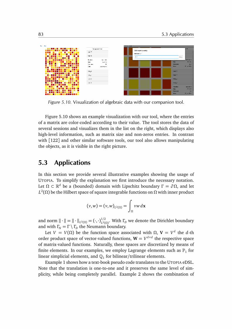
83 5.3 Applications
Figure 5.10. Visualization of algebraic data with our companion tool.
Figure 5.10 shows an example visualization with our tool, where the entriesof a matrix are color-coded according to their value. The tool stores the data ofseveral sessions and visualizes them in the list on the right, which displays alsohigh-level information, such as matrix size and non-zeros entries. In contrastwith [122] and other similar software tools, our tool also allows manipulatingthe objects, as it is visible in the right picture.
5.3 Applications
In this section we provide several illustrative examples showing the usage ofUTOPIA. To simplify the explanation we first introduce the necessary notation.Let ⌦ ⇢ Rd be a (bounded) domain with Lipschitz boundary � = @⌦, and letL2(⌦) be the Hilbert space of square integrable functions on⌦with inner product
(v, w) = (v, w)L2(⌦) =Z
⌦
vw dx
and norm k · k = k · kL2(⌦) = (·, ·)1/2L2(⌦). With �D we denote the Dirichlet boundaryand with �N = � \ �D the Neumann boundary.
Let V = V (⌦) be the function space associated with ⌦, V = V d the d-thorder product space of vector-valued functions, W = V d⇥d the respective spaceof matrix-valued functions. Naturally, these spaces are discretized by means offinite elements. In our examples, we employ Lagrange elements such as P1 forlinear simplicial elements, and Q1 for bilinear/trilinear elements.
Example 1 shows how a text-book pseudo code translates to the UTOPIA eDSL.Note that the translation is one-to-one and it preserves the same level of sim-plicity, while being completely parallel. Example 2 shows the combination of
84 5.3 Applications
UTOPIA solvers with the MOOSE library. Interoperability is achieved by meansof the SNESAdapter. This interface uses the PETSc SNES data structure to passinformation about objective functions and their derivatives to the non-linear so-lution method. Consequently, it can be easily used with other FEM libraries builton top of PETSc, such as the MOOSE framework [24].
Example 3 shows how to use our eDSL for specifying a non-linear anisotropic-Poisson problem with solution-dependent diffusion coefficients. In this examplethe coefficient-function f is specified using the C++11 lambda function rhs_fun.Example 4 shows, how to specify an initial value problem,
@ u(x , t)/@ t = h(t, u(x , t), . . .)
with u(x , t0) = u0(x), by exploiting the UTOPIA primitive dt for identifying thetime derivative. From the variational formulation we automatically extract theupdate function h which is used in a time integrator, such as the explicit Euler orthe Runge-Kutta.
The last two examples show mixed formulations which can be interpreted asthe variational problem: find u 2 V,� 2W:
a(u, v) + b(�, v) = k(v)b(q, u) + g(�,q) = d(q) 8v 2 V,q 2W,
where a, b, g are bilinear-forms, and k, d are linear-forms. This problem is ismirrored in the code by the corresponding block linear system:
A BBT G
�u�
�=kd
�.
Example 5 shows how to assemble such mixed finite element problem derivedfrom a least-squares functional [102]which ensures the ellipticity of the resultinglinear operator. Similarly, Example 6 shows how to assemble a least-squareslinear-elasticity problem. Note that in this example, the UTOPIA eDSL is used ina larger environment which deals with contact problems [33].

85 5.3 Applications
Example 1: Preconditioned conjugate gradientDescription
Algorithm taken from [126].
Pseudo-code and parallel code
Vector r, d, q, s;double delta_new, delta_0, delta_old;double alpha, beta;
i 0 int i = 0;r b�Ax r = b - A * x;d M�1r solve(M, r, d);�new rT d delta_new = dot(r, d);�0 �new delta_0 = delta_new;While i < imax ^�new > "
2�0 while(i < i_max && delta_new > eps_2 * delta_0) {q Ad q = A * d;
↵ �new
dT qalpha = delta_new/dot(d, q);
x x+↵d x += alpha * d;
If i is divisible by 50 if(i % 50 == 0)r b�Ax r = b - A * x;
Else elser r�↵q r -= alpha * q;
s M�1r solve(M, r, s);�old �new delta_old = delta_new;�new rT s delta_new = dot(r, s);
� �new
�oldbeta = delta_new/delta_old;
d s+ �d d = s + beta * d;i i + 1 ++i;
}

86 5.3 Applications
Example 2: Phase field fractureDescription
Find u 2 Vt , c 2 Mt , and � 2Qt , such that�[(1� c)2 + k]�+0 ���0 ,rv
�= (t,v)�N
(lrc,rq) + (� , q) = (lrc · n, q)�N✓@ c@ t� 1⌘
⌦� + 2(1� c)
+0gc� c
l
↵+, m
◆= 0,
8v 2 Vt , 8q 2 Qt , 8m 2 Mt , where t 2 [0, T], c 2 [0, 1], gc , l,⌘, k 2 R, hxi+ = (|x | + x)/2is the ramp function, and the �+ and �� super-scripts respectively represent the positive andnegative parts of the stress; see [97]. We perform our experiment in a parallelepipedal domain,and we discretize Vt with Pd
1 elements, and both Mt and Qt with P1 elements. The computationis performed in a displacement-driven context where the rate of change u on the y-axis is 10�5 onthe top side and zero on the bottom side. We use a linear elastic material with Lamé parameters� = 12, µ= 8, and phase-field parameters ⌘ = 5⇥ 10�4, l = 0.022, and k = 10�8.
Code
auto direct_solver = make_shared<LUDecomposition<Matrix, Vector>>();auto smoother = make_shared<GaussSeidel<Matrix, Vector>>();
// initialization of preconditioner, setting up interpolation operatorsMultigrid<Matrix, Vector> mg(smoother, direct_solver);mg.init(move(interpolation_operators));mg.set_max_iter(1); mg.set_cycle_type(2);
// iterative linear solver with MG as a preconditionerConjugateGradient<Matrix, Vector> cg; cg.set_preconditioner(make_ref(mg));
// non-linear solverNewton<Matrix, Vector> solver(cg);solver.set_line_search_strategy(make_shared<Backtracking<Matrix, Vector>>());
// interface between MOOSE and utopia non-linear solversSNESAdapter<Matrix, Vector> fun(snes); solver.solve(fun, x);
Simulation
uy = 0 uy = 5.9⇥ 10�3 uy = 6.3⇥ 10�3 uy = 7.4⇥ 10�3
Crack pattern for different values of uy . The color represents the solution for the phase-fieldparameter c, from the unbroken state c = 0 (gray) to the fully broken state c = 1 (red).

87 5.3 Applications
Example 3: Non-linear anisotropic Poisson problemDescription
Find u 2 V :(1/(u2 + 0.1)Aru,rv) = ( f , v),
8v 2 V , where f 2 V , u|@⌦ = g, and A 2 Rd⇥d .We perform our simulation with two connected cubes, with paramters f = 10kxk2�5 for x 2 ⌦,g = 0, A= diag(10,0.1, 1), and we discretize V with Q1 elements.
Code
int dim = 2;// anisotropic diffusion tensorMatrix A = identity(dim, dim);A.set(0, 0, 10);A.set(1, 1, 0.1);A.set(2, 2, 1);
// right-hand sidestd::function<void(const Point &p, Scalar &ret)>rhs_fun = [dim](const Point &p, Scalar &ret) -> void {// right-hand side function code...
};
auto f = coeff(rhs_fun);
// solutionauto u_k = interpolate( coeff(1.0), Vh, make_ref(solution_vec) );
// bilinear formauto bf = integral( dot(1./(pow2(u_k) + coeff(0.1)) * A * grad(u), grad(v)) );
// linear formauto lf = integral(dot(f, v));
Simulation
Visualization of the solution u from different persectives.
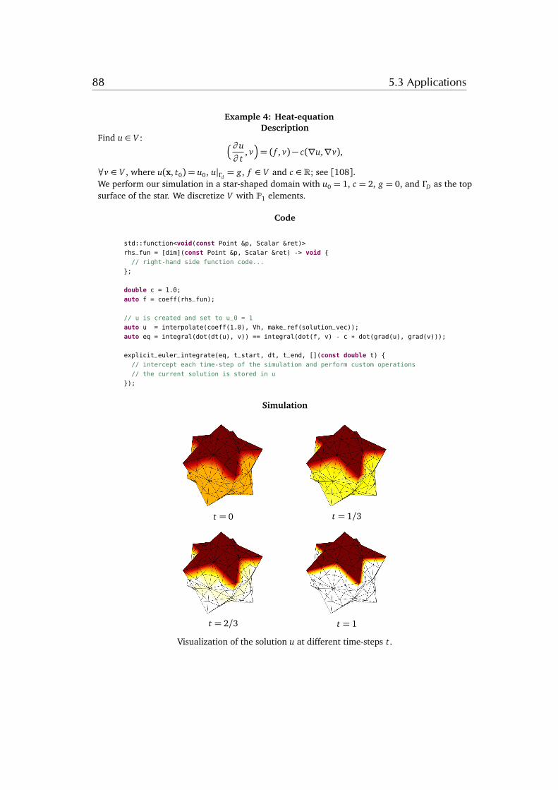
88 5.3 Applications
Example 4: Heat-equationDescription
Find u 2 V : Ä@ u@ t
, vä= ( f , v)� c(ru,rv),
8v 2 V , where u(x, t0) = u0, u|�d = g, f 2 V and c 2 R; see [108].We perform our simulation in a star-shaped domain with u0 = 1, c = 2, g = 0, and �D as the topsurface of the star. We discretize V with P1 elements.
Code
std::function<void(const Point &p, Scalar &ret)>rhs_fun = [dim](const Point &p, Scalar &ret) -> void {// right-hand side function code...
};
double c = 1.0;auto f = coeff(rhs_fun);
// u is created and set to u_0 = 1auto u = interpolate(coeff(1.0), Vh, make_ref(solution_vec));auto eq = integral(dot(dt(u), v)) == integral(dot(f, v) - c * dot(grad(u), grad(v)));
explicit_euler_integrate(eq, t_start, dt, t_end, [](const double t) {// intercept each time-step of the simulation and perform custom operations// the current solution is stored in u
});
Simulation
t = 0 t = 1/3
t = 2/3 t = 1
Visualization of the solution u at different time-steps t.
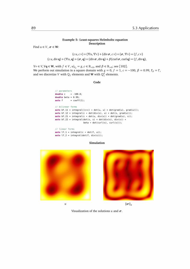
89 5.3 Applications
Example 5: Least-squares Helmholtz equationDescription
Find u 2 V , � 2W:
(c u, c v) + (ru,rv) + (div�, c v) + (�,rv) = ( f , c v)(c u, divq) + (ru,q) + (�,q) + (div�, divq) + �(curl�, curlq) = ( f , divq),
8v 2 V,8q 2W, with f 2 V , u|�D = g, c 2 R<0, and � 2 R>0; see [102].We perform out simulation in a square domain with g = 0, f = 1, c = �100, � = 0.99, �D = � ,and we discretize V with Q1 elements and W with Qd
1 elements.
Code
// parametersdouble c = -100.0;double beta = 0.99;auto f = coeff(1);
// bilinear formsauto bf_11 = integral((c*c) * dot(u, u) + dot(grad(u), grad(u)));auto bf_12 = integral(c * dot(div(s), u) + dot(s, grad(u)));auto bf_21 = integral(c * dot(u, div(s)) + dot(grad(u), s));auto bf_22 = integral(dot(s, s) + dot(div(s), div(s)) +
beta * dot(curl(s), curl(s)));
// linear formsauto lf_1 = integral(c * dot(f, u));auto lf_2 = integral(dot(f, div(s)));
Simulation
u k�k2
Visualization of the solutions u and �.

90 5.3 Applications
Example 6: Linear elasticity with least-squares finite elementsDescription
Find u 2 V,� 2W
("(u),"(v))� (A�,"(v)) = 0
�("(u),A q) + (div�, divq) + (A�,A q) = �(f, divq),
8v 2 V and 8q 2W, where f 2 V, u|�D = g, �|�D = z, "(w) = (rw+ (rw)T )/2, and
A : Rd⇥d ! Rd⇥d , A� = 12µ(� � �
d�+ 2µ(tr�)I)
is the inverse strain-stress relationship tensor and �,µ 2 R are the Lamé paramters; see [23]. Wesimulate the contact betweend two unit sized squares with � = 1,µ = 1, and f = 0. We specifythe boundary conditions g = �[0.2, 0.2] on the top side, g = [0.2,0.2] on the bottom, z = 0 onthe left and right sides. Contact conditions are resolved according as explained in Section 2.3.1.We discretize V with Q2
1 elements and W with Q2⇥21 elements.
Code
auto A = stress_strain_rel_tensor(dim, mu, lambda);auto f = vec_coeff(force);
auto e = 0.5 * (transpose(grad(u)) + grad(u));auto As = A * s;
// bilinear formsauto b11 = integral(inner(e, e));auto b12 = integral(-inner(As, e));auto b21 = integral(-inner(e, As));auto b22 = integral(inner(div(s), div(s)) + inner(As, As));
// linear formsauto l1 = integral(inner(vec_coeff(0., 0.), u));auto l2 = integral(-inner(f, div(s)));
Simulation
Input kuk2 �11 �12 �21 �22
Viusalization of the solutions u and �.
91 5.4 Chapter conclusion
5.4 Chapter conclusion
UTOPIA is a unified C++ eDSL for non-linear algebra and finite element assem-bly following the philosophy of separation of model and computation. With aMATLAB-like look-and-feel, our eDSL supports existing state-of-the-art software li-braries, code generation and expression templates. UTOPIA has lower barriers toentry to parallel computing, since it provides purposefully partial parallelization,data-distribution and memory-location transparency. Moreover, UTOPIA providessimple debugging routines to visualize both numerical and structural data. Sincesolution methods, both linear and non-linear, are a fundamental building blockof any scientific software our eDSL is extended to provide a coherent interfacefor supporting a large variety of strategies. These features are shown in severalexamples of solution strategies and variational formulations in finite element as-sembly.
One current major performance issue in our back-end implementations ismemory allocation. Though this issue can be addressed specifically in each back-end, we plan to develop an independent mechanism to automatically solve thisproblem. Our idea is to provide memory pools which reduce the amount of allo-cations by reusing intermediate representations. Another performance improve-ment consists of providing primitives to handle sparsity explicitly, for instanceallocating a sparse matrix with the same sparsity pattern as another one (e.g., m2= sparse(sparsity(m1))). Finally, a minor issue of UTOPIA is the compilationtime due to the heavy use of template types. This issue will be attenuated by ex-ploiting C++ modules which are currently being standardized for future versionof C++ [38].
A relevant MATLAB primitive is index-sets. This primitive allows accessingtensorial entries based on a set of indices. Unfortunately, this feature is not yetavailable in UTOPIA hence it will be added in the near future. We plan to ex-tend the eDSL with primitives to allow transfer of discrete fields [81] for non-conforming domain decomposition methods [13; 137; 105]. Another interestinglanguage feature is variational inequalities which allows specifying obstacle orcontact problems [34]. The UTOPIA eDSL already contains a basic prototype ofsymbolic differentiation [39; 56], we aim to improve it and add it to the finiteelement eDSL. When the symbolic version does not apply, we intend to includeautomatic differentiation mechanisms [4].
Finally, we plan to integrate and develop new back-ends for both the alge-bra and the finite element assembly. This will allow to benchmark the differentlibraries within the same framework.

92 5.4 Chapter conclusion
Chapter 6
Numerical experiments
In this chapter we look into the runtime performance of our parallel informa-tion transfer algorithm (Section 6.1), and we observe the numerical behaviorof solving the Poisson problem discretized with our parametric finite elementdiscretization (Section 6.2).
6.1 Parallel transfer
The first contribution of the parallel approach presented in this Chapter 3 is toenable for really complex and difficult simulation scenarios to be handled. Nev-ertheless, in this section we illustrate scaling studies in the weak-scaling andstrong-scaling settings. We also illustrate particular corner cases where the ap-proach does not perform at its best, and provide considerations on output sensi-tivity and its effect on scaling. Being a method for handling an output-sensitiveproblem, the issue of scaling should neither be addressed nor observed as in stan-dard and ideal scenarios. We measure scaling/speed-up by s = tB/tP , where tP
is the time of the run with P processes and tB is the time of the base run with Bprocesses.
In our experiment we measure the cost of the assembly of the transfer oper-ator starting when the input mesh is received, hence the measurement includessearching, computing intersections, generating quadrature formulas, computingthe local integrals, and delivering the two coupling operators in their sparse ma-trix representation.
As approximation spaces we have chosen linear Lagrangian finite-elementspaces. As a measure of the output we count the number of intersections whichis equivalent to the number of evaluated integrals. The cost of integration mayvary with respect to the shape of the intersection.
93
94 6.1 Parallel transfer
In order to provide an estimate of the cost of the assembly of the transferoperator in comparison to a standard mass matrix assembly we performed anexperiment in serial with the same routines that we use in our parallel numer-ical experiments. The finite element assembly is performed in a generic soft-ware framework which allows for mixed formulations with customizable quadra-ture formulas, and our measurements are performed for a meshed cube T with297 316 elements. For assembling the transfer operator we use mass-matrix as-sembly calls with Petrov-Galerkin formulation (different trial and test spaces) andspecial quadrature formulas which are generated as explained in Section 2.3. Weconsider the computational time of the assembly procedure a standard mass ma-trix and compare it with the computational time for computing the pseudo-L2
projection operator. This particular transfer operator is constructed for transfer-ring between equal spaces both associated with the same mesh, hence resultingin an identity matrix. The measurements include the computational time associ-ated with the intersection detection, intersection computation, quadrature pointsgeneration, and assembly. The observed ratio between the assembly time of thetransfer operator and the assembly time of the mass matrix is approximately 15,and the larger portion of the cost is due to intersection computation and theassembly. The measurements of our experiments are tagged and organized asfollows:
• Create adapters: the cost of creating the adapter representations from theprovided geometric data. An adapter allows representing an element andits related mesh data in a suitable format for the library code abstractions.In order to this these adapters include meta-information such as tags, do-main markers, and geometric information such as AABBs and k-DOPs.
• Build tree/detection: the cost of constructing the octree, searching for match-ing remote nodes, generating index-sets for handling both the nodes andthe geometric data.
• Load-balancing: the cost of linearizing the local trees and scheduling thenarrow-phase detection.
• Organize dependencies: organization and communication of the actual ge-ometric data.
• Match and re-balance: cost of the narrow-phase detection, and re-balancing.Here no actual intersection is computed, only bounding-volume matchingis performed.
95 6.1 Parallel transfer
• Computation: intersection computation and assembly.
We can consider all the measurements except the computation, as the overheadwhich results in using our algorithm.
6.1.1 Hardware
The studies have been performed at the Swiss Supercomputing Center (CSCS)on a Cray XC40 with the following specification: 1256 Compute Nodes with 2Intel® Xeon® E5-2690 v3 @ 2.60GHz (12 cores each, 24 virtual cores each withhyperthreading enabled); Theoretical Peak Performance 1.254 Petaflops; Mem-ory Capacity per node 64 GB (1192 nodes) and 128 GB (64 fat nodes, bigmem);Memory Bandwidth per node up to 137 GB/s per node; Total System Memory82.5 TB DDR3; Peak Network Bisection Bandwidth of 4.5 TB/s; Parallel File Sys-tem Peak Performance of 50 GB/s;
6.1.2 Weak-scaling experiments
With weak scaling, we investigate how the framework behaves, with respect tocomputational time, when increasing the number of processors, and keeping theamount of computation per process fixed. The problem is output-sensitive, whichmeans that the computational complexity depends on the size of the output, mak-ing it difficult, for most scenarios, to study scaling in a fair way by just controllingthe size of the input.
Hence, we study weak scaling in the simplest scenario, depicted in Figure 6.1.We have a stack of parallelepipeds, each parallelepiped has two resolutions a finemesh and a coarse mesh. The partitions of coarse and fine meshes are randomlydistributed also with respect to each other. Hence, intersecting elements of thefine mesh and coarse mesh are likely to be owned by different processes, thusstored in different memory address spaces. In this setting, we assemble the trans-fer operator for transferring from the coarse space to the fine space.
In Figure 6.1, we see the scaling results for this experiment in two resolutions.In Figure 6.2, we have a detailed illustration of the medium size experiment.
6.1.3 Strong-scaling experiments
With strong scaling, we investigate how the framework behaves with respect tocomputational time, when increasing the number of processes, and keeping thetotal size of the problem fixed. The charts in Figure 6.3 and Figure 6.4, illustrate

96 6.1 Parallel transfer
p1 p2
p3
p0
Stacked decomposed multi-gridparallelepipeds. Color represents
processes.
101 102 103 104 105
0.20.40.60.8
1
Number of processesSc
alin
g
IdealMedium (153 022)Large (641 141)
Figure 6.1. Weak scaling with different resolutions. Medium: per process10 923 input, 43 691 output. Large: per process 153 022 input, 641 141 output.See Figure 6.2 for more details about the medium size experiment.
12 96 768 1 536 3 072 6 144 12 2880
20
40
60
80
Seco
nds
Search and balancingComputation
Create adapters 0.05 0.05 0.05 0.05 0.05 0.05 0.05Build tree/detection 0.26 0.44 1.68 1.54 2.10 3.59 10.78
Load-balancing 0.00 0.00 0.00 0.00 0.00 0.01 0.00Organize dependencies 0.19 0.21 0.24 0.24 0.24 0.30 0.31
Match and re-balance 0.20 0.20 0.24 0.24 0.24 0.31 0.25Computation 24.07 28.66 29.39 33.73 36.74 45.58 63.25
Total 24.78 29.58 31.63 35.83 39.40 49.87 74.60Processes 12 96 768 1536 3 072 6 144 12 288
Tree-depth 5 5 5 6 6 6 6Input size (log2) 17 20 23 24 25 26 27
Output size (log2) 19 22 25 26 27 28 29
Figure 6.2. Volume projections: weak scaling experiment. The x axis describethe number of processes. The computational times is measured in seconds. Theinput is about 10 200 tetrahedral elements per process. Search and balancing
includes all the measurements except the computation.
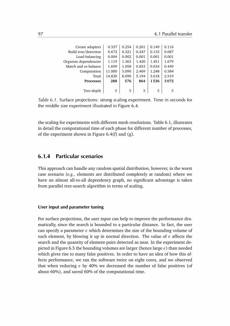
97 6.1 Parallel transfer
Create adapters 0.337 0.254 0.201 0.149 0.116Build tree/detection 0.672 0.321 0.247 0.133 0.087
Load-balancing 0.004 0.002 0.001 0.001 0.001Organize dependencies 1.119 1.363 1.420 1.451 1.679
Match and re-balance 1.699 1.058 0.853 0.634 0.449Computation 11.000 5.090 2.469 1.248 0.584
Total 14.830 8.090 5.194 3.618 2.919Processes 288 576 864 1 536 3 072
Tree-depth 5 5 5 5 5
Table 6.1. Surface projections: strong scaling experiment. Time in seconds forthe middle size experiment illustrated in Figure 6.4.
the scaling for experiments with different mesh resolutions. Table 6.1, illustratesin detail the computational time of each phase for different number of processes,of the experiment shown in Figure 6.4(f) and (g).
6.1.4 Particular scenarios
This approach can handle any random spatial distribution, however, in the worstcase scenario (e.g., elements are distributed completely at random) where wehave an almost all-to-all dependency graph, no significant advantage is takenfrom parallel tree-search algorithm in terms of scaling.
User input and parameter tuning
For surface projections, the user input can help to improve the performance dra-matically, since the search is bounded to a particular distance. In fact, the usercan specify a parameter ✏ which determines the size of the bounding volume ofeach element, by blowing it up in normal direction. The value of ✏ affects thesearch and the quantity of element-pairs detected as near. In the experiment de-picted in Figure 6.5 the bounding volumes are larger (hence large ✏) than neededwhich gives rise to many false positives. In order to have an idea of how this af-fects performance, we ran the software twice on eight cores, and we observedthat when reducing ✏ by 40% we decreased the number of false positives (ofabout 60%), and saved 60% of the computational time.
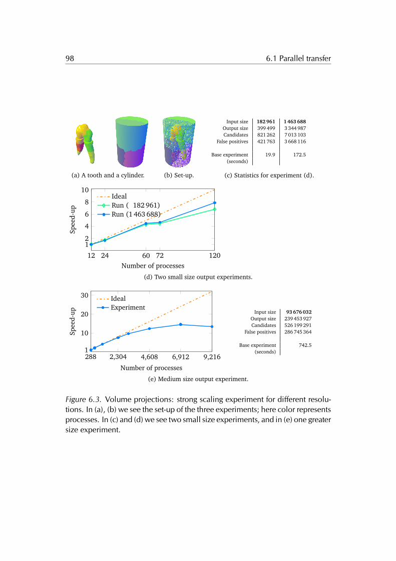
98 6.1 Parallel transfer
Input size 182 961 1 463 688Output size 399 499 3 344 987Candidates 821 262 7 013 103
False positives 421 763 3 668 116
Base experiment 19.9 172.5(seconds)
(a) A tooth and a cylinder. (b) Set-up. (c) Statistics for experiment (d).
12 24 60 72 12012
4
6
8
10
Number of processes
Spee
d-up
IdealRun ( 182 961)Run (1 463 688)
(d) Two small size output experiments.
288 2,304 4,608 6,912 9,2161
10
20
30
Number of processes
Spee
d-up
IdealExperiment
Input size 93 676 032Output size 239 453 927Candidates 526 199 291
False positives 286 745 364
Base experiment 742.5(seconds)
(e) Medium size output experiment.
Figure 6.3. Volume projections: strong scaling experiment for different resolu-tions. In (a), (b) we see the set-up of the three experiments; here color representsprocesses. In (c) and (d) we see two small size experiments, and in (e) one greatersize experiment.

99 6.1 Parallel transfer
(a) Example multi-bodycontact simulation.
(b) Bounding volumehierarchy constructed
by the algorithm.
(c) Detected contactboundary and gaps.
48 24 36 48 60 72 96 108 1321
10
20
30
Number of processes
Spee
d-up
IdealExperiment Volume elements 11 608 960
Surface adapters 529 648Output size 73 207Candidates 1 249 892
False positives 1 176 685
Base experiment 9.6(seconds)
(d) Small.
288 576 864 1536
1234
6
Number of processes
Spee
d-up
IdealExperiment Volume elements 742 973 440
Surface adapters 8 474 368Output size 929 688Candidates 156 505 837
False positives 155 576 149
Base experiment 14.8(seconds)
(e) Medium.
1,920 3,840 7,680
1
2
3
4
Number of processes
Spee
d-up
IdealExperiment Volume elements 5 943 787 520
Surface adapters 33 897 472Output size 3 464 544Candidates 2 163 911 881
False positives 2 160 447 333
Base experiment 35.3(seconds)
(f) Large.
Figure 6.4. Surface projections: strong scaling experiment with different resolu-tions. In (a), (b), and (c) is depicted the context of the experiment. The coloring:in (a) it is the Von-Mises stress, in (b) it represent the process. The scaling resultsexclusively include the cost of computing the transfer operator related quantities.In experiment (d), above 60 processes we can see the search costs taking over,and the total time stagnates at around 0.5 seconds. Similarly, in experiment (f),the search occupies the 70% of the total time.

100 6.2 Parametric finite elements with bijective mappings
Surface proximity detectionproblem.
Bounding volume hierarchy. Detail of the geometric surfaceprojection.
Figure 6.5. Predicting the contact region: when there is a-priori knowledgeabout the problem, the scope of the search can be reduced for saving computa-tional time. Color represent processes.
6.1.5 Scaling and output-sensitivity
The main reason for the observed scaling behavior, in both strong and weak scal-ing studies, is mainly due to imbalance and synchronization waiting time in thesearch phase. The imbalance is due to the initial geometric set-up, when themeshes are distributed in an unbalanced way as for instance in the scenario pre-sented in Section 6.1.3, or the actual output of the search is strongly unbalanced.In fact, since we are treating an output-sensitive problem, the actual cost of thesearch is unknown a-priori and depends directly on the output, i.e., the numberof candidate intersections, which is directly related to the spatial location of themeshes. Once the intersection candidates are found, and we have the neces-sary knowledge, the assembly procedure can be performed in a more balancedway. However, also the actual assembly might be subject to unavoidable im-balance depending on the actual computed intersection polytopes and numberof quadrature points which are generated on each process. A possible solutionmight be to re-balance again after the computation of the intersections.
6.2 Parametric finite elements with bijective mappings
We focus our study on (mostly) super-parametric discretizations based on com-posite mean value mappings (Section 2.5.1) and its approximations (Section 4.3)with linear Lagrange elements (P1). For our experiments the analytical solutionis unknown, hence we estimate it by computing a reference solution u 2 X 1
1(T f )on a very fine mesh T f . To evaluate the quality of our discretization and thestandard discretization, we compute different solutions uh for several mesh sizes
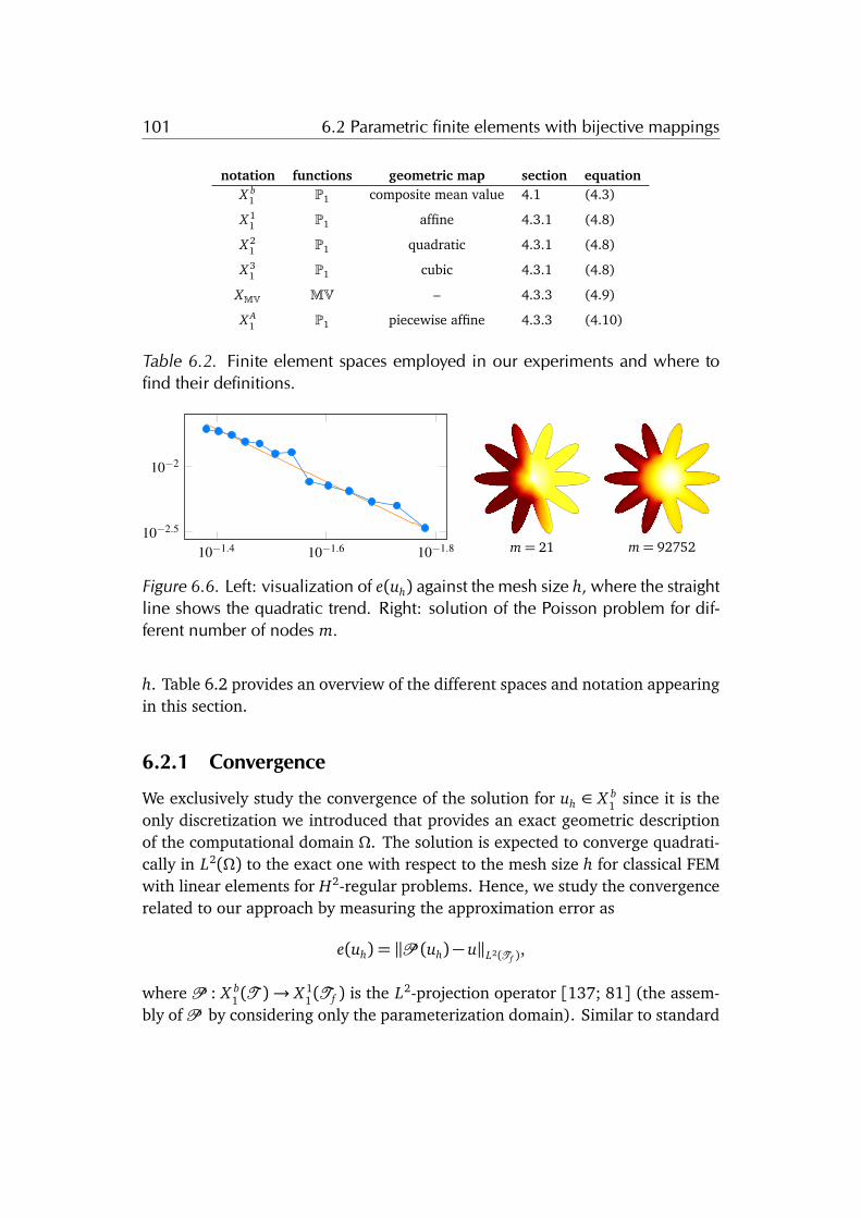
101 6.2 Parametric finite elements with bijective mappings
notation functions geometric map section equationX b
1 P1 composite mean value 4.1 (4.3)
X 11 P1 affine 4.3.1 (4.8)
X 21 P1 quadratic 4.3.1 (4.8)
X 31 P1 cubic 4.3.1 (4.8)
XMV MV – 4.3.3 (4.9)
X A1 P1 piecewise affine 4.3.3 (4.10)
Table 6.2. Finite element spaces employed in our experiments and where tofind their definitions.
10
�1.810
�1.610
�1.410
�2.5
10
�2
m= 21 m= 92752
Figure 6.6. Left: visualization of e(uh) against the mesh size h, where the straightline shows the quadratic trend. Right: solution of the Poisson problem for dif-ferent number of nodes m.
h. Table 6.2 provides an overview of the different spaces and notation appearingin this section.
6.2.1 Convergence
We exclusively study the convergence of the solution for uh 2 X b1 since it is the
only discretization we introduced that provides an exact geometric descriptionof the computational domain ⌦. The solution is expected to converge quadrati-cally in L2(⌦) to the exact one with respect to the mesh size h for classical FEMwith linear elements for H2-regular problems. Hence, we study the convergencerelated to our approach by measuring the approximation error as
e(uh) = kP (uh)� ukL2(T f ),
where P : X b1 (T )! X 1
1(T f ) is the L2-projection operator [137; 81] (the assem-bly of P by considering only the parameterization domain). Similar to standard

102 6.2 Parametric finite elements with bijective mappings
Figure 6.7. Mesh refinement without shape recovery. Even at fine resolution(last image) we do not recover the original shape (blue polygon).
FEM, our method shows a quadratic convergence behaviour for the Poisson prob-lem, as illustrated in the plot in Figure 6.6. Despite the fact that the computationis always performed in the exact geometry, the approximation error is not zerobecause of the piecewise polynomial approximation of the solution, which is vis-ible for a mesh with small m and disappears for larger m.
6.2.2 Comparison
We compare our discretization with the standard finite element discretization fora simple 2D problem (Figure 6.8), an extreme 2D problem (Figure 6.9), and for arealistic 3D shape (Figure 6.10). Since for the standard finite element discretiza-tion, the boundary of T differs from ⌦, we measure
r(uh) =����kuhkL2(T )kukL2(T f )
� 1
����
to estimate the approximation error [91].In classical finite element simulations the original shape is usually not recov-
ered when performing mesh refinement as shown in Figure 6.7. For this reason,r(uh) does not converge to zero for the standard solution, while our approachconverges (left plots in Figures 6.8, 6.9, and 6.10).
In order to better understand this behaviour, we measure the actual geometricdeviation with
s(T ) = k1kL2(T ),which corresponds to the volume of the mesh (note that s(T ) is computed bysumming the entries of the mass-matrix). We compute the volume by meansof numerical quadrature, which might introduce errors, since our discretizationconsists of warped elements. For the standard discretization, when refining themesh without recovering the shape, the volume trivially stays constant. Hence,in order to have a fair comparison, we increase the shape accuracy while refin-ing the mesh to ensure that the shape of the domain also converges to the exact
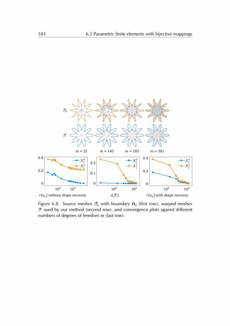
103 6.2 Parametric finite elements with bijective mappings
T0
T
m= 21 m= 143 m= 183 m= 381
102 103
0
0.2
0.4X b
1X 1
1
102 103
0
0.1
0.2X b
1X 1
1
102 1030
0.2
0.4X b
1X 1
1
r(uh) without shape recovery. s(T ). r(uh) with shape recovery.
Figure 6.8. Source meshes T0 with boundary ⇥0 (first row), warped meshesT used by our method (second row), and convergence plots against differentnumbers of degrees of freedom m (last row).

104 6.2 Parametric finite elements with bijective mappings
T0
T
m= 21 m= 136 m= 375 m= 1791
103 104
0
0.05
0.1
0.15
0.2
X b1
X 11
102 103 104
0
0.1
0.2 X b1
X 11
102 103 104
0
0.05
0.1
0.15 X b1
X 11
r(uh) without shape recovery. s(T ). r(uh) with shape recovery.
Figure 6.9. Source meshes T0 with boundary ⇥0 (first row), warped meshesT used by our method (second row), and convergence plots against differentnumbers of degrees of freedom m (last row).
⇥0 ⇥ n= 42 n= 80 n= 194 n= 644 n= 1611
103 104 105
0
0.2
0.4
0.6
0.8
X b1
X 11
103 104 105
0
0.1
0.2
0.3
0.4X b
1X 1
1
103 104 105
0
0.2
0.4
0.6
0.8X b
1X 1
1
r(uh) without shape recovery. s(T ). r(uh) with shape recovery.
Figure 6.10. Convergence plots against different numbers of degrees of freedomm for a 3D experiment.
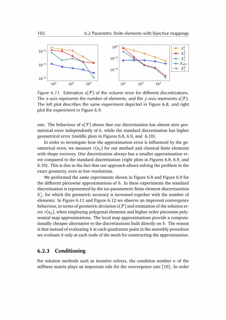
105 6.2 Parametric finite elements with bijective mappings
102 103 10410�6
10�4
10�2
101 102 103
10�4
10�2
100X 1
1X 2
1X 3
1XMVX A
1
Figure 6.11. Estimation s(T ) of the volume error for different discretizations.The x -axis represents the number of elements, and the y-axis represents s(T ).The left plot describes the same experiment depicted in Figure 6.8, and rightplot the experiment in Figure 6.9.
one. The behaviour of s(T ) shows that our discretization has almost zero geo-metrical error independently of h, while the standard discretization has highergeometrical error (middle plots in Figures 6.8, 6.9, and 6.10).
In order to investigate how the approximation error is influenced by the ge-ometrical error, we measure r(uh) for our method and classical finite elementswith shape recovery. Our discretization always has a smaller approximation er-ror compared to the standard discretization (right plots in Figures 6.8, 6.9, and6.10). This is due to the fact that our approach allows solving the problem in theexact geometry, even at low resolutions.
We performed the same experiments shown in Figure 6.8 and Figure 6.9 forthe different piecewise approximations of b. In these experiments the standarddiscretization is represented by the iso-parameteric finite element discretizastionX 1
1 , for which the geometric accuracy is increased together with the number ofelements. In Figure 6.11 and Figure 6.12 we observe an improved convergencebehaviour, in terms of geometric deviation s(T ) and estimation of the solution er-ror r(uh), when employing polygonal elements and higher order piecewise poly-nomial map approximations. The local map approximations provide a computa-tionally cheaper alternative to the discretizations built directly on b. The reasonis that instead of evaluating b at each quadrature point in the assembly procedurewe evaluate it only at each node of the mesh for constructing the approximation.
6.2.3 Conditioning
For solution methods such as iterative solvers, the condition number of thestiffness matrix plays an important role for the convergence rate [10]. In order

106 6.2 Parametric finite elements with bijective mappings
102 103 10410�4
10�2
100
101 102 103
10�2
10�1
100 X 11
X 21
X 31
XMVX A
1
Figure 6.12. Estimation r(uh) of the solution error for different discretizations.The x -axis represents the number of elements, and the y-axis represents r(uh).The left plot describes the same experiment depicted in Figure 6.8, and rightplot the experiment in Figure 6.9.
to understand how our discretization affects the condition number, we compute for the discrete Laplace operator L with respect to different mesh sizes h for bothour discretization and the standard one. Because of the influence of the bijectivemapping b, as shown in (4.6), our discretization has a slightly larger conditionnumber. Figure 6.13 shows that (L) behaves similarly for both discretizationswhich suggests that iterative solvers perform nearly as well for our discretizationas for the standard one.
6.2.4 Convergence of the multigrid method with parametric fi-nite elements
We observe the average convergence rate of the multigrid method applied to dif-ferent parameterizations for reaching a residual Mf� Lu with magnitude 10�12.We compare it to a semi-geometric multigrid method where we construct the
10�0.2 10�0.4 10�0.6
101
102
103
X b1
X 11
100 10�0.5 10�1
102
103
X b1
X 11
Figure 6.13. Condition number of the discrete Laplace operator (L) against themesh size h for the examples in Figure 6.8 (left) and Figure 6.9 (right).

107 6.2 Parametric finite elements with bijective mappings
coarse levels of the multigrid hierarchy by exploiting the pseudo-L2-projectionoperator introduced in Section 2.2. For generating such hierarchy we first com-pute the axis-aligned bounding-box (AABB) of the input mesh T = T L. Then,we compute T 1 by meshing the AABB in such a way that the number of elementsof T 1 is smaller than the number of elements in TL by a factor of (2d)L�1, whered is the spatial dimension. When building T 1 we make sure that its elementshave an aspect ratio close to one. We generate the intermediate L � 2 meshesby (uniform) refinement of T 0. Then, we compute the pseudo-L2-projection op-erator IL from the coarse space Vh(TL�1) to the fine space Vh(TL) as explainedin Section 2.3. We compute the prolongation operators for the lower levels asfor standard geometric multigrid methods. We define this hierarchy of spaces asHP . An overview of the geometric objects involved is shown in Figure 6.14.
Let us recall the spaces and hierarchies of the parametric discretization de-fined in Section 4.4. The hierarchyH k
p is composed by the spaces X kp(T l) where
p represents the order of the polynomial basis functions defined in the referenceelement and k the polynomial order of the geometric transformation.
The hierarchyH Ap is composed by the spaces X A
p where p represents the orderof the polynomial basis functions defined in the reference element and A repre-sents the piece-wise geometric map defined for each element of the fine levelmesh.
WithHMV we denote the hierarchy of polygonal finite element spaces.For our experiments we select different type of domains with several level of
details, smooth and non-smooth features. However, as explained in Section 4.3.1a valid piecewise k-th order polynomial map bk is not always available. Hence,we restrict our numerical evaluation to examples which allows constructing suchmap. We observe the average convergence rate
⇢ = n�1nX
q=1
kLuq �Mfk/kLuq�1 �Mfk,
where uq is the solution at the q-th iteration, n is the number of iterations, and u0
is the initial guess. Our observations are made with respect to different resolutionof both the input mesh and the solution to the Poisson problem (4.1).
We observe that the hierarchies H Ap and H k
p consistently appear to providethe same convergence rate for all experiments (Figure 6.15 and Table 6.3). ThehierarchiesHMV andHP instead display degraded convergence rates dependingon the geometric set-up. The loss of convergence appears to manifests itselffor HMV when the shape of the elements is highly distorted for many layersaround the boundary, and forHP when the domain has an extremely oscillatory
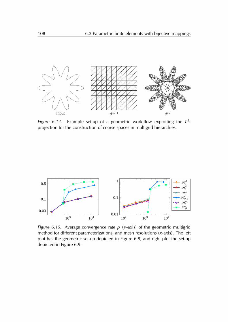
108 6.2 Parametric finite elements with bijective mappings
Input T L�1 T L
Figure 6.14. Example set-up of a geometric work-flow exploiting the L2-projection for the construction of coarse spaces in multigrid hierarchies.
103 104
0.03
0.1
0.5
102 103 1040.01
0.1
1 H 11H 21H 31HMVH A
1HP
Figure 6.15. Average convergence rate ⇢ (y-axis) of the geometric multigridmethod for different parameterizations, and mesh resolutions (x -axis). The leftplot has the geometric set-up depicted in Figure 6.8, and right plot the set-updepicted in Figure 6.9.
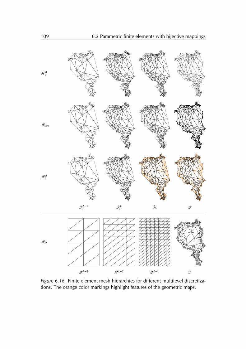
109 6.2 Parametric finite elements with bijective mappings
H 31
HMV
H A1
T L�10 T L
0 T0 T
HP
T L�3 T L�2 T L�1 TFigure 6.16. Finite element mesh hierarchies for different multilevel discretiza-tions. The orange color markings highlight features of the geometric maps.

110 6.2 Parametric finite elements with bijective mappings
# elements # d.o.f. fine / coarse # iterations convergence rate ⇢
H 11
300 196/61 8 0.0261 200 691/196 11 0.0734 800 2 581/691 12 0.103
19 200 9 961/2 581 14 0.135
H 21 /H 3
1
300 196/61 8 0.0271 200 691/196 11 0.0714 800 2 581/691 12 0.101
19 200 9 961/2 581 14 0.135
HMV75 568/61 10 0.069
300 1 068/196 18 0.2081 200 2 131/691 22 0.2784 800 4 993/2 581 25 0.334
19 200 13 600/9 961 31 0.425
H A1
300 196/61 8 0.0271 200 691/196 11 0.0724 800 2 581/691 12 0.103
19 200 9 961/2 581 14 0.135
HP433 330 / 104 7 0.019669 448 / 153 31 0.406
2 272 1 250 / 493 57 0.6116 999 3 637 / 1 881 57 0.613
16 987 8 692 / 4 753 60 0.628
Table 6.3. Comparison of performance of the multigrid method with respect todifferent discretizations for the example shown in Figure 6.16.

111 6.3 Chapter conclusion
shape (right plot Figure 6.15). Additionally, the convergence rate of the multigridmethod is slightly worse when increasing the number of degrees of freedom forbothHMV andHP .
A more typical scenario and the different geometric approximations and meshhierarchies are illustrated Figure 6.16. In this scenario, the multgrid method hasconvergence rates below 0.7 for all discretization, however the variants withparametric finite elements display a much better convergence behavior, as it canbe observed in Table 6.3.
6.3 Chapter conclusion
We performed numerical experiments including weak-scaling and strong-scalingof our parallel algorithm for the variational transfer of discrete fields. We ob-served that most of the computational effort of our approach goes into comput-ing the numerical quadrature, and for a large number of processes goes intofinding intersection candidates. We investigated performance drivers. The timeneeded for communication of the actual geometric data is comparably small, andthe main issue is the load-balancing which is challenged by the output-sensitivenature of the problem.
We studied the behaviour of our parametric finite element discretization basedon mean-value mappings and its local approximations with respect to the Poissonproblem. Through numerical experimentation we show that our super-parametricdiscretization generally has a lower approximation error compared to the stan-dard one, due to the higher geometric accuracy, without significant changes onthe conditioning of the discrete operators. We observed that our discretizationdoes not affects the performance of the multigrid method for super-parametriccase. For the case of polygonal finite elements based on mean-value coordinateswe observed a shape dependent degrading behaviour.

112 6.3 Chapter conclusion
Chapter 7
Conclusion
We investigated what we consider to be key issues related to complex geometricinteractions in parallel multi-physics simulations. For dealing with such issues,we proposed a completely parallel strategy for transferring discrete fields be-tween arbitrarily distributed finite element meshes and its applications. Witha relatively small computational time overhead our strategy allows to simplifythe simulation work-flow even for very complex mesh distribution scenarios. Westudied the performance and the limitations of our strategy through detailednumerical experiments, and we provided several example application scenarios.We open-sourced and integrated our algorithms with the MFEM and the LIBMESH
libraries.We proposed a new parametric finite element discretization that allows de-
coupling the accuracy of the shape from the choice of the approximation space infinite element simulations. This separation allows for high flexibility with respectto the geometric objects in the simulation work-flow. We studied our discretiza-tion with several numerical experiments illustrating both promising results andlimitations. Even if our discretization is based on mean-value mappings and theirlocal approximations, we believe that further investigations may reveal more ef-ficient and effective way of generating finite element discretizations.
We have discussed current trends and our idea for the development of sci-entific libraries. We instantiated our ideas with the UTOPIA library for which weprovided a detailed description of its design and rationales. The UTOPIA libraryis public available as an open-source project.
A topic which has been only partially covered is the automatic determinationof contact patches in contact problems. In fact, we have not covered this topicfor parallel computations. In parallel settings the automatic determination ofmaster and slave roles of contact patches may be a very useful tool which would
113

114
simplify the simulation work-flow significantly.
Bibliography
[1] M. AIGNER, C. HEINRICH, B. JÜTTLER, E. PILGERSTORFER, B. SIMEON,AND A.-V. VUONG, Swept volume parameterization for isogeometric analy-sis, Springer, 2009.
[2] P. R. AMESTOY, I. S. DUFF, J. KOSTER, AND J.-Y. L’EXCELLENT, A fully asyn-chronous multifrontal solver using distributed dynamic scheduling, SIAMJournal on Matrix Analysis and Applications, 23 (2001), pp. 15–41.
[3] D. N. ARNOLD, F. BREZZI, B. COCKBURN, AND L. D. MARINI, Unified analysisof discontinuous galerkin methods for elliptic problems, SIAM Journal onNumerical Analysis, 39 (2002), pp. 1749–1779.
[4] P. AUBERT, N. DI CÉSARÉ, AND O. PIRONNEAU, Automatic differentiation inc++ using expression templates and. application to a flow control problem,Computing and Visualization in Science, 3 (2001), pp. 197–208.
[5] U. AYACHIT, The ParaView guide : updated for ParaView version 4.3, Kit-ware, 2015.
[6] M. BADER, Space-filling curves: an introduction with applications in scien-tific computing, vol. 9, Springer Science & Business Media, 2012.
[7] S. BALAY, W. D. GROPP, L. C. MCINNES, AND B. F. SMITH, Efficient man-agement of parallelism in object oriented numerical software libraries, inModern Software Tools in Scientific Computing, E. Arge, A. M. Bruaset,and H. P. Langtangen, eds., Birkhäuser Press, 1997, pp. 163–202.
[8] W. BANGERTH, R. HARTMANN, AND G. KANSCHAT, Deal.ii & mdash; ageneral-purpose object-oriented finite element library, ACM Transactions onMathematical Software, 33 (2007).
[9] P. BASTIAN, G. BUSE, AND O. SANDER, Infrastructure for the coupling of Dunegrids, in Proceedings of ENUMATH 2009, Springer, 2010, pp. 107–114.
115

116 Bibliography
[10] K.-J. BATHE AND E. L. WILSON, Numerical methods in finite element analysis,AMC, 10 (1976), p. 12.
[11] Y. BAZILEVS, C. MICHLER, V. CALO, AND T. HUGHES, Isogeometric variationalmultiscale modeling of wall-bounded turbulent flows with weakly enforcedboundary conditions on unstretched meshes, Computer Methods in AppliedMechanics and Engineering, 199 (2010).
[12] H. BEN DHIA, Multiscale mechanical problems: the Arlequin method,Comptes Rendus de l’Academie des Sciences Series IIB Mechanics PhysicsAstronomy, 326 (1998), pp. 899–904.
[13] C. BERNARDI, Y. MADAY, AND F. RAPETTI, Basics and some applications ofthe mortar element method, GAMM-Mitt., 28 (2005), pp. 97–123.
[14] F. BERTRAND, S. MUNZENMAIER, AND G. STARKE, First-order system leastsquares on curved boundaries: Higher-order Raviart–Thomas elements,SIAM Journal on Numerical Analysis, 52 (2014), pp. 3165–3180.
[15] F. BERTRAND, S. MUNZENMAIER, AND G. STARKE, First-order system leastsquares on curved boundaries: Lowest-order Raviart–Thomas elements,SIAM Journal on Numerical Analysis, 52 (2014), pp. 880–894.
[16] J. BEY, Tetrahedral grid refinement, Computing, 55 (1995), pp. 355–378.
[17] D. BRAESS, Finite elements. Theory, fast solvers and applications in solidmechanics, Cambridge University Press, 2007.
[18] J. H. BRAMBLE, J. E. PASCIAK, AND O. STEINBACH, On the stability of the L2-projections in H1, Mathematics of Computation, 71 (2002), pp. 147–156.
[19] J. BRANDT, P. J. GUO, J. LEWENSTEIN, AND S. R. KLEMMER, Opportunis-tic programming: How rapid ideation and prototyping occur in practice, inProceedings of the 4th International Workshop on End-user Software En-gineering, ACM, 2008, pp. 1–5.
[20] S. BRENNER AND R. SCOTT, The Mathematical Theory of Finite ElementMethods, vol. 15, Springer-Verlag New York, 2008.
[21] S. C. BRENNER AND I. TUTORIAL, Geometric multigrid methods, 2010.
[22] W. L. BRIGGS, V. E. HENSON, AND S. F. MCCORMICK, A multigrid tutorial(2nd ed.), Society for Industrial and Applied Mathematics, 2000.
117 Bibliography
[23] Z. CAI AND G. STARKE, Least-squares methods for linear elasticity, SIAMJournal on Numerical Analysis, 42 (2004), pp. 826–842.
[24] P. CHAKRABORTY, Y. ZHANG, M. R. TONKS, AND S. B. BINER, Multi-scalemodeling of inter-granular fracture in uo2, tech. rep., Idaho National Lab-oratory (INL), Idaho Falls, ID (United States), 2015.
[25] H. CHILDS, E. BRUGGER, B. WHITLOCK, J. MEREDITH, S. AHERN, D. PUG-MIRE, K. BIAGAS, M. MILLER, C. HARRISON, G. H. WEBER, H. KRISHNAN,T. FOGAL, A. SANDERSON, C. GARTH, E. W. BETHEL, D. CAMP, O. RÜBEL,M. DURANT, J. M. FAVRE, AND P. NAVRÁTIL, VisIt: An End-User Tool For Visu-alizing and Analyzing Very Large Data, in High Performance Visualization–Enabling Extreme-Scale Scientific Insight, Taylor and Francis, Oct 2012,pp. 357–372.
[26] P. G. CIARLET AND P.-A. RAVIART, Interpolation theory over curved elements,with applications to finite element methods, Computer Methods in AppliedMechanics and Engineering, 1 (1972), pp. 217–249.
[27] K. L. CLARKSON, R. E. TARJAN, AND C. J. VAN WYK, A fast las vegas algorithmfor triangulating a simple polygon, Discrete & Computational Geometry, 4(1989), pp. 423–432.
[28] M. COUR CHRISTENSEN, U. VILLA, A. ENGSIG-KARUP, AND P. VASSILEVSKI,Nonlinear multigrid solver exploiting amge coarse spaces with approxima-tion properties, tech. rep., Lawrence Livermore National Laboratory, 2016.
[29] M. DE BERG, O. C. M. VAN KREVELD, AND M. OVERMARS, ComputationalGeometry Algorithms and Applications, Springer-Verlag Italia, 2008.
[30] A. DE BOER, A. VAN ZUIJLEN, AND H. BIJL, Review of coupling methodsfor non-matching meshes, Computer Methods in Applied Mechanics andEngineering, 196 (2007), pp. 1515–1525.
[31] Z. DEVITO, N. JOUBERT, F. PALACIOS, S. OAKLEY, M. MEDINA, M. BARRIEN-TOS, E. ELSEN, F. HAM, A. AIKEN, K. DURAISAMY, E. DARVE, J. ALONSO, AND
P. HANRAHAN, Liszt: A domain specific language for building portable mesh-based pde solvers, in Proceedings of 2011 International Conference forHigh Performance Computing, Networking, Storage and Analysis, ACM,2011, pp. 9:1–9:12.
118 Bibliography
[32] T. DICKOPF, Multilevel methods based on non-nested meshes, PhD thesis,Friedrich-Wilhelms University of Bonn, 2010.
[33] T. DICKOPF AND R. KRAUSE, Efficient simulation of multi-body contact prob-lems on complex geometries: A flexible decomposition approach using con-strained minimization, International Journal for Numerical Methods in En-gineering, 77 (2009), pp. 1834–1862.
[34] T. DICKOPF AND R. KRAUSE, Weak information transfer between non-matching warped interfaces, in Domain Decomposition Methods in Sci-ence and Engineering XVIII, M. Bercovier, M. Gander, R. Kornhuber, andO. Widlund, eds., vol. 70, Springer, 2009, pp. 283–290.
[35] T. DICKOPF AND R. KRAUSE, Monotone multigrid methods based on para-metric finite elements, tech. rep., ICS, USI, may 2011.
[36] T. DICKOPF AND R. KRAUSE, Evaluating local approximations of the L2-orthogonal projection between non-nested finite element spaces, NumericalMathematics: Theory, Methods, and Applications, 7 (2014).
[37] W. DÖRFLER AND M. RUMPF, An adaptive strategy for elliptic problems in-cluding a posteriori controlled boundary approximation, Mathematics ofComputation of the American Mathematical Society, 67 (1998), pp. 1361–1382.
[38] G. DOS REIS, M. HALL, AND G. NISHANOV, A module system for c++(revision2), 2014.
[39] A. DÜRRBAUM, W. KLIER, AND H. HAHN, Comparison of automatic and sym-bolic differentiation in mathematical modeling and computer simulation ofrigid-body systems, Multibody System Dynamics, 7 (2002), pp. 331–355.
[40] M. ECK, T. DEROSE, T. DUCHAMP, H. HOPPE, M. LOUNSBERY, AND W. STUET-ZLE, Multiresolution analysis of arbitrary meshes, in Proceedings of the22Nd Annual Conference on Computer Graphics and Interactive Tech-niques, ACM, 1995, pp. 173–182.
[41] C. ERICSON, Real-Time Collision Detection (The Morgan Kaufmann Series inInteractive 3D Technology), Morgan Kaufmann Publishers Inc., 2004.
[42] A. P. ERIKSON AND K. ÅSTRÖM, Analysis for Science, Engineering and Be-yond: The Tribute Workshop in Honour of Gunnar Sparr held in Lund, May8-9, 2008, Springer Berlin Heidelberg, 2012, pp. 93–141.

119 Bibliography
[43] A. ERN AND J.-L. GUERMOND, Theory and practice of finite elements,vol. 159, Springer Science & Business Media, 2013.
[44] L. C. EVANS, Partial differential equations, American Mathematical Society,1998.
[45] P. E. FARRELL, Galerkin projection of discrete fields via supermesh construc-tion, PhD thesis, Imperial College London, September 2009.
[46] P. E. FARRELL AND J. MADDISON, Conservative interpolation between volumemeshes by local galerkin projection, Computer Methods in Applied Mechan-ics and Engineering, 200 (2011), pp. 89–100.
[47] B. FLEMISCH AND B. I. WOHLMUTH, Stable Lagrange multipliers for quadri-lateral meshes of curved interfaces in 3D, Computer Methods in AppliedMechanics and Engineering, 196 (2007), pp. 1589–1602.
[48] M. S. FLOATER, Mean value coordinates, Computer Aided Geometric De-sign, 20 (2003), pp. 19–27.
[49] M. J. GANDER AND C. JAPHET, An algorithm for non-matching grid projec-tions with linear complexity, in Domain Decomposition Methods in Scienceand Engineering XVIII, Springer, 2009, pp. 185–192.
[50] D. GASTON, C. NEWMAN, G. HANSEN, AND D. LEBRUN-GRANDIE, Moose:A parallel computational framework for coupled systems of nonlinear equa-tions, Nuclear Engineering and Design, 239 (2009), pp. 1768–1778.
[51] F. H. GEISLER, The CHARITE artificial disc: design history, FDA IDE studyresults, and surgical technique., Clinical neurosurgery, 53 (2006), pp. 223–228.
[52] F. GRECO AND N. SUKUMAR, Derivatives of maximum-entropy basis func-tions on the boundary: Theory and computations, International Journal forNumerical Methods in Engineering, 94 (2013), pp. 1123–1149.
[53] D. GROEN, S. J. ZASADA, AND P. V. COVENEY, Survey of multiscale and mul-tiphysics applications and communities, Computing in Science & Engineer-ing, 16 (2014), pp. 34–43.
[54] C. GROSS AND R. KRAUSE, On the convergence of recursive Trust–Regionmethods for multiscale non-linear optimization and applications to non-linear mechanics, SIAM Journal on Numerical Analysis, 47 (2009),pp. 3044–3069.
120 Bibliography
[55] G. GUENNEBAUD, B. JACOB, ET AL., Eigen v3, 2010.
[56] B. GUENTER, Efficient symbolic differentiation for graphics applications,ACM Transactions on Graphics, 26 (2007), p. 108.
[57] W. HACKBUSCH, Multi-grid methods and applications, vol. 4, Springer-Verlag, 1985.
[58] M. HEROUX, R. BARTLETT, V. H. R. HOEKSTRA, J. HU, T. KOLDA,R. LEHOUCQ, K. LONG, R. PAWLOWSKI, E. PHIPPS, A. SALINGER, H. THORN-QUIST, R. TUMINARO, J. WILLENBRING, AND A. WILLIAMS, An overview oftrilinos, Tech. Rep. SAND2003–2927, Sandia National Laboratories, 2003.
[59] M. A. HEROUX, J. M. WILLENBRING, AND R. HEAPHY, Trilinos developersguide, Tech. Rep. SAND2003–1898, Sandia National Laboratories, 2007.
[60] C. HESCH AND P. BETSCH, A comparison of computational methods for largedeformation contact problems of flexible bodies, ZAMM - Journal of AppliedMathematics and Mechanics, 86 (2006), pp. 818–827.
[61] C. HESCH AND P. BETSCH, Transient three-dimensional domain decompo-sition problems: Frame-indifferent mortar constraints and conserving inte-gration, International Journal for Numerical Methods in Engineering, 82(2010), pp. 329–358.
[62] C. HESCH AND P. BETSCH, Isogeometric analysis and domain decompositionmethods, Computer Methods in Applied Mechanics and Engineering, 213(2012), pp. 104–112.
[63] C. HESCH AND P. BETSCH, An object oriented framework: From flexible multi-body dynamics to fluid-structure interaction, The 2nd Joint InternationalConference on Multibody System Dynamics, (2012).
[64] C. HESCH, A. GIL, A. A. CARREÑO, J. BONET, AND P. BETSCH, A mortarapproach for fluid–structure interaction problems: Immersed strategies fordeformable and rigid bodies, Computer Methods in Applied Mechanics andEngineering, 278 (2014), pp. 853–882.
[65] M. HOLST, FEtk: Finite Element ToolKit, 2003.
[66] K. HORMANN AND N. SUKUMAR, Maximum entropy coordinates for arbitrarypolytopes, Computer Graphics Forum, 27 (2008), pp. 1513–1520.
121 Bibliography
[67] T. J. HUGHES, J. A. COTTRELL, AND Y. BAZILEVS, Isogeometric analysis: CAD,finite elements, NURBS, exact geometry and mesh refinement, ComputerMethods in Applied Mechanics and Engineering, 194 (2005), pp. 4135–4195.
[68] J. R. HUMPHREY, D. K. PRICE, K. E. SPAGNOLI, A. L. PAOLINI, AND E. J.KELMELIS, Cula: hybrid gpu accelerated linear algebra routines, in SPIEdefense, security, and sensing, 2010, pp. 770502–770502.
[69] K. IGLBERGER, G. HAGER, J. TREIBIG, AND U. RÜDE, Expression templatesrevisited: a performance analysis of current methodologies, SIAM Journalon Scientific Computing, 34 (2012), pp. C42–C69.
[70] A. JACOBSON, Bijective mappings with generalized barycentric coordinates:a counterexample, tech. rep., Department of Computer Science, ETHZurich, 2012.
[71] P. JOLIVET, V. DOLEAN, F. E. E. HECHT, F. E. E. NATAF, C. PRUD HOMME, AND
N. SPILLANE, High performance domain decomposition methods on mas-sively parallel architectures with freefem++, Journal of Numerical Math-ematics, 20 (2012), pp. 287–302.
[72] W. JOPPICH AND M. KÜRSCHNER, MpCCI - a tool for the simulation of coupledapplications, Concurrency and Computation: Practice and Experience, 18(2006), pp. 183–192.
[73] T. JU, S. SCHAEFER, AND J. WARREN, Mean value coordinates for closedtriangular meshes, ACM Transactions on Graphics, 24 (2005), pp. 561–566.
[74] KHRONOS OPENCL WORKING GROUP, The OpenCL Specification, version1.0.29, 2008.
[75] N. KIKUCHI AND J. T. ODEN, Contact problems in elasticity: a study of vari-ational inequalities and finite element methods, vol. 8, siam, 1988.
[76] B. S. KIRK, J. W. PETERSON, R. H. STOGNER, AND G. F. CAREY, libmesh: ac++ library for parallel adaptive mesh refinement/coarsening simulations,Engineering with Computers, 22 (2006), pp. 237–254.
[77] T. KOLEV, MFEM: Modular finite element methods, 2016.
122 Bibliography
[78] D. KRAUSE, K. FACKELDEY, AND R. KRAUSE, A parallel multiscale simula-tion toolbox for coupling molecular dynamics and finite elements, in Sin-gular Phenomena and Scaling in Mathematical Models, M. Griebel, ed.,Springer International Publishing, 2014, pp. 327–346.
[79] D. KRAUSE AND R. KRAUSE, MACI. A Parallel Multiscale Simulation Toolboxfor Coupling Molecular Dynamics and Finite Elements, 2014.
[80] R. KRAUSE AND O. SANDER, Automatic construction of boundaryparametrizations for geometric multigrid solvers, Computing and Visual-ization in Science, 9 (2006), pp. 11–22.
[81] R. KRAUSE AND P. ZULIAN, A parallel approach to the variational transferof discrete fields between arbitrarily distributed finite element meshes, SIAMJournal on Scientific Computing, 38 (2016), pp. C307–C333.
[82] B. P. LAMICHHANE, R. P. STEVENSON, AND B. I. WOHLMUTH, Higher ordermortar finite element methods in 3D with dual Lagrange multiplier bases,Numerische Mathematik, 102 (2005), pp. 93–121.
[83] A. W. LEE, W. SWELDENS, P. SCHRÖDER, L. COWSAR, AND D. DOBKIN, Maps:Multiresolution adaptive parameterization of surfaces, in Proceedings of the25th annual conference on Computer graphics and interactive techniques,1998, pp. 95–104.
[84] S. LEFEBVRE AND H. HOPPE, Perfect spatial hashing, in ACM SIGGRAPH2006 Papers, ACM, 2006, pp. 579–588.
[85] B. LI, X. LI, K. WANG, AND H. QIN, Surface mesh to volumetric spline con-version with generalized polycubes, IEEE Transactions on Visualization andComputer Graphics, 19 (2013), pp. 1539–1551.
[86] Q. LI, K. ITO, Z. WU, C. S. LOWRY, I. LOHEIDE, AND P. STEVEN, Comsolmultiphysics: A novel approach to ground water modeling, Groundwater,47 (2009), pp. 480–487.
[87] H. LIAN, S. P. A. BORDAS, R. SEVILLA, AND R. N. SIMPSON, Recent Develop-ments in CAD/analysis Integration, ArXiv e-prints, (2012).
[88] A. LOGG, Automating the finite element method, Archives of ComputationalMethods in Engineering, 14 (2007), pp. 93–138.

123 Bibliography
[89] A. LOGG AND G. N. WELLS, DOLFIN: automated finite element computing,CoRR, abs/1103.6248 (2011).
[90] K. LONG, R. KIRBY, AND B. VAN BLOEMEN WAANDERS, Unified embeddedparallel finite element computations via software-based fréchet differenti-ation, SIAM Journal on Scientific Computing, 32 (2010), pp. 3323–3351.
[91] X. LUO, M. S. SHEPHARD, AND J.-F. REMACLE, The influence of geometricapproximation on the accuracy of high order methods, Rensselaer SCORECreport, 1 (2001).
[92] R. C. MARTIN, More C++ gems, vol. 17, Cambridge University Press, 2000.
[93] T. MARTIN AND E. COHEN, Volumetric parameterization of complex ob-jects by respecting multiple materials, Computers & Graphics, 34 (2010),pp. 187–197.
[94] A. MASSING, M. G. LARSON, A. LOGG, AND M. E. ROGNES, An overlappingmesh finite element method for a fluid-structure interaction problem, arXivpreprint, (2013).
[95] J. MELENK AND B. WOHLMUTH, On residual-based a posteriori error esti-mation in hp-fem, Advances in Computational Mathematics, 15 (2001),pp. 311–331.
[96] B. MEYER, Applying design by contract, IEEE Transactions on Computers,25 (1992), pp. 40–51.
[97] C. MIEHE, F. WELSCHINGER, AND M. HOFACKER, Thermodynamically con-sistent phase-field models of fracture: Variational principles and multi-fieldfe implementations, International Journal for Numerical Methods in Engi-neering, 83 (2010).
[98] J. MOSLER AND M. ORTIZ, Variational h-adaption in finite deformation elas-ticity and plasticity, International Journal for Numerical Methods in Engi-neering, 72 (2007), pp. 505–523.
[99] J. NICKOLLS, I. BUCK, M. GARLAND, AND K. SKADRON, Scalable parallelprogramming with CUDA, Queue, 6 (2008), pp. 40–53.
[100] C. NVIDIA, Cublas library, 2008.
124 Bibliography
[101] J. O’ROURKE, Computational Geometry in C, Cambridge University Press,1998.
[102] A. PEHLIVANOV, G. CAREY, AND P. VASSILEVSKI, Least-squares mixed finiteelement methods for non-selfadjoint elliptic problems: I. error estimates, Nu-merische Mathematik, 72 (1996), pp. 501–522.
[103] K. B. PETERSEN, M. S. PEDERSEN, ET AL., The matrix cookbook, 2008.
[104] C. PRUD HOMME, V. CHABANNES, V. DOYEUX, M. ISMAIL, A. SAMAKE, AND
G. PENA, Feel++: A computational framework for galerkin methods and ad-vanced numerical methods, in ESAIM: Proceedings, vol. 38, 2012, pp. 429–455.
[105] M. A. PUSO, A 3D mortar method for solid mechanics, International Journalfor Numerical Methods in Engineering, 59 (2004).
[106] M. A. PUSO AND T. A. LAURSEN, A mortar segment-to-segment contactmethod for large deformation solid mechanics, Computer Methods in Ap-plied Mechanics and Engineering, 193 (2004).
[107] L. QI AND J. SUN, A nonsmooth version of newton’s method, Mathematicalprogramming, 58 (1993), pp. 353–367.
[108] A. QUARTERONI, Numerical Models for Differential Problems, Springer,2009.
[109] A. QUARTERONI AND A. VALLI, Domain decomposition methods for partialdifferential equations, Clarendon Press, 1999.
[110] M. RANDRIANARIVONY, Tetrahedral transfinite interpolation with b-patchfaces: construction and regularity, INS Preprint, 803 (2008).
[111] M. RANDRIANARIVONY, On transfinite interpolations with respect to convexdomains, Computer Aided Geometric Design, 28 (2011), pp. 135–149.
[112] F. RATHGEBER, D. A. HAM, L. MITCHELL, M. LANGE, F. LUPORINI, A. T. T.MCRAE, G. BERCEA, G. R. MARKALL, AND P. H. J. KELLY, Firedrake: au-tomating the finite element method by composing abstractions, CoRR,abs/1501.01809 (2015).
[113] S. P. REISS, The challenge of helping the programmer during debugging, inSoftware Visualization (VISSOFT), 2014 Second IEEE Working Confer-ence on, 2014, pp. 112–116.

125 Bibliography
[114] S. L. RIDGWAY, Finite element techniques for curved boundaries, PhD thesis,Massachusetts Institute of Technology, 1973.
[115] S. L. RIDGWAY, Interpolated boundary conditions in the finite elementmethod, SIAM Journal on Numerical Analysis, 12 (1975), pp. 404–427.
[116] M. RIVI, L. CALORI, G. MUSCIANISI, AND V. SLAVNIC, In-situ visualization:State-of-the-art and some use cases, PRACE White Paper, (2012).
[117] K. RUPP, Gpu-accelerated non-negative matrix factorization for text mining,in NVIDIA GPU Technology Conference, 2012, p. 77.
[118] K. RUPP, F. RUDOLF, AND J. WEINBUB, A discussion of selected vienna-librariesfor computational science, 2013.
[119] C. SANDERSON AND R. CURTIN, Armadillo: a template-based C++ libraryfor linear algebra, The Journal of Open Source Software, 1 (2016).
[120] T. SCHNEIDER AND K. HORMANN, Smooth bijective maps between arbitraryplanar polygons, Computer Aided Geometric Design, (2015).
[121] T. SCHNEIDER, K. HORMANN, AND M. S. FLOATER, Bijective composite meanvalue mappings, Computer Graphics Forum, 32 (2013), pp. 137–146.
[122] T. SCHNEIDER, P. ZULIAN, M. R. AZADMANESH, R. KRAUSE, AND
M. HAUSWIRTH, Vestige: A visualization framework for engineeringgeometry-related software, Proceedings of VISSOFT (3rd IEEE WorkingConference on Software Visualization), (2015).
[123] R. SEIDEL, A simple and fast incremental randomized algorithm for com-puting trapezoidal decompositions and for triangulating polygons, Compu-tational Geometry, 1 (1991), pp. 51–64.
[124] R. SEVILLA, S. FERNÁNDEZ-MÉNDEZ, AND A. HUERTA, Nurbs-enhanced finiteelement method (nefem), Archives of Computational Methods in Engineer-ing, 18 (2011), pp. 441–484.
[125] J. SHEWCHUK, What is a good linear finite element? interpolation, condi-tioning, anisotropy, and quality measures (preprint), University of Califor-nia at Berkeley, 73 (2002).
[126] J. R. SHEWCHUK, An introduction to the conjugate gradient method withoutthe agonizing pain, 1994.
126 Bibliography
[127] A. H. STROUD AND D. SECREST, Gaussian Quadrature Formulaes, Prentice-Hall, 1966.
[128] N. SUKUMAR AND E. A. MALSCH, Recent advances in the construction ofpolygonal finite element interpolants, Archives of Computational Methodsin Engineering, 13 (2006).
[129] H. SUNDAR, R. S. SAMPATH, AND G. BIROS, Bottom-up construction and 2: 1balance refinement of linear octrees in parallel, SIAM Journal on ScientificComputing, 30 (2008), pp. 2675–2708.
[130] I. E. SUTHERLAND AND G. W. HODGMAN, Reentrant polygon clipping, Com-mun. ACM, 17 (1974), pp. 32–42.
[131] J. TSUDA, Practical rigid body physics for games, in ACM SIGGRAPH ASIA2009 Courses, ACM, 2009, pp. 14:1–14:83.
[132] L. R. TURNER, Inverse of the vandermonde matrix with applications, NASAtechnical note D-3547, (1996).
[133] T. VELDHUIZEN, Expression templates, 1995.
[134] J. WALTER AND M. KOCH, BOOST C++ Libraries, 2009.
[135] Q. WANG, H. ZHOU, AND D. WAN, Numerical simulation of wind turbineblade-tower interaction, Journal of Marine Science and Application, 11(2012), pp. 321–327.
[136] J. WLOKA, Partial differential equations, Cambridge university press, 1987.
[137] B. I. WOHLMUTH, A mortar finite element method using dual spaces forthe Lagrange multiplier, SIAM Journal on Numerical Analysis, 38 (1998),pp. 989–1012.
[138] B. I. WOHLMUTH AND R. H. KRAUSE, Monotone multigrid methods on non-matching grids for nonlinear multibody contact problems, SIAM Journal onScientific Computing, 25 (2003), pp. 324–347.
[139] S. XIAO AND T. BELYTSCHKO, A bridging domain method for coupling con-tinua with molecular dynamics, Computer Methods in Applied Mechanicsand Engineering, 193 (2004), pp. 1645–1669.
127 Bibliography
[140] D. XUE, L. DEMKOWICZ, ET AL., Control of geometry induced error in hp finiteelement (fe) simulations. i. evaluation of fe error for curvilinear geometries,Int. J. Numer. Anal. Model, 2 (2005), pp. 283–300.
[141] B. YANG AND T. A. LAURSEN, A large deformation mortar formulation of selfcontact with finite sliding, Computer Methods in Applied Mechanics andEngineering, 197 (2008), pp. 756–772.
[142] P. ZULIAN, A. KOPANICÁKOVÁ, AND T. SCHNEIDER, Utopia: A c++ embeddeddomain specific language for scientific computing, 2016.
Related Documents