Geometry Algorithms “Geometry Algorithms” http://people.sc.fsu.edu/∼jburkardt/presentations/ asa geometry 2011.pdf .......... ISC4221C-01: Algorithms for Science Applications II .......... John Burkardt Department of Scientific Computing Florida State University Spring Semester 2011 1 / 144

Welcome message from author
This document is posted to help you gain knowledge. Please leave a comment to let me know what you think about it! Share it to your friends and learn new things together.
Transcript
Geometry Algorithms
“Geometry Algorithms”http://people.sc.fsu.edu/∼jburkardt/presentations/
asa geometry 2011.pdf..........
ISC4221C-01:Algorithms for Science Applications II
..........John Burkardt
Department of Scientific ComputingFlorida State University
Spring Semester 2011
1 / 144

Geometry Algorithms
Overview
The Points on a Line
Points NOT on a Line
Estimating Integrals over an Interval
Triangles and their Properties
Triangulating a Polygon
The Convex Hull
Triangulating a Point Set by Delaunay
Estimating Integrals over a Triangle
Conclusion
2 / 144
OVERVIEW: Geometry
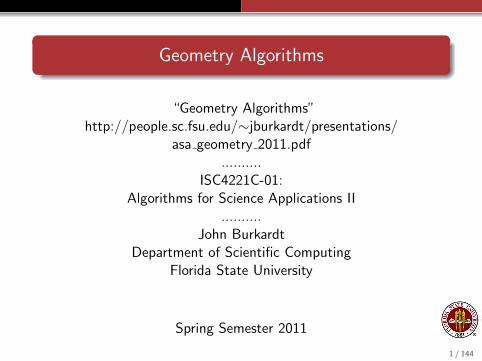
We use computational geometry to decompose an object intosimple shapes that can be displayed in a computer animation.
3 / 144
OVERVIEW: Geometry
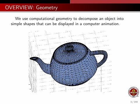
Computational geometry builds models that can be stressed orcrashed for realistic tests.
4 / 144
OVERVIEW: Geometry
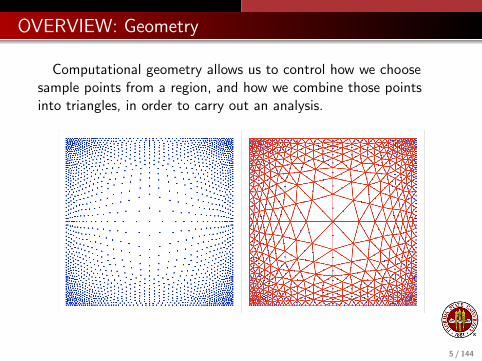
Computational geometry allows us to control how we choosesample points from a region, and how we combine those pointsinto triangles, in order to carry out an analysis.
5 / 144
OVERVIEW: Geometry
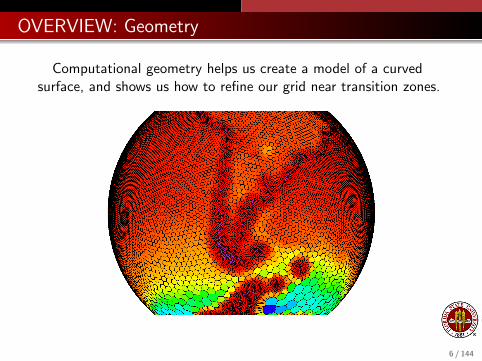
Computational geometry helps us create a model of a curvedsurface, and shows us how to refine our grid near transition zones.
6 / 144
OVERVIEW: Geometry
The objects we just saw were broken into simpler objects.This is the basis of computational geometry.
To do all these wonderful things with computational geometry, wego back to the basic geometric objects, figure out how toimplement them on a computer, and then teach the computer,step by step, the rules that allow us to assemble and understandmore complicated objects.
Over two weeks, we will be lucky to study some properties ofpoints, lines, triangles, and triangular meshes.
Computational geometry can easily fill a semester of study.
7 / 144
OVERVIEW: Geometric Tasks
We will sample common computational geometry tasks:
measurement of length, area, volume, distance, direction,orientation;
discretization of curves and surfaces;
indexing or parameterizing the parts of an object;
nearest object;
intersection of two objects;
containment of one object in another;
parallel and orthogonal components;
decomposition of an object into basic objects;
transformations: shift, rotate, reflect, shear an object;
sampling a random object in a set.
8 / 144
Geometry Algorithms
Overview
The Points on a Line
Points NOT on a Line
Estimating Integrals over an Interval
Triangles and their Properties
Triangulating a Polygon
The Convex Hull
Triangulating a Point Set by Delaunay
Estimating Integrals over a Triangle
Conclusion
9 / 144
POINTS: Locations
The “atoms” of geometry are points; every geometric object canbe thought of as a collection of points that satisfy some property.
Depending on what we are studying, our geometry can be 1D, 2D,3D or a higher, abstract dimension. Unless we are studying aspecial surface like the sphere, we will usually think of a point interms of its Cartesian coordinates. For example, the coordinates ofa 3D point might be described as (x , y , z); If we have severalpoints, we subscript the coordinates, so that z2 would be the zcoordinate of the second point.
Computationally, it is preferable to store the coordinates of a pointin a single variable; for instance, p = [x , y , z ].
MATLAB allows a vector to be row or column vector. I preferpoints to be described as column vectors. In that case, we’d writeeither p = [x ; y ; z ] or else p = [x , y , z ]′.
10 / 144

POINTS: What is a Line?
A line is the infinite set of points which...how do we explain it?We know what a line is when we look at one, but that’s not goodenough.
We know that two points, say p1 and p2, determine a line; wemight say the line goes through one point and towards the other.So any point on the line might be described by the process ofstarting at p1 and going “in the direction” of p2. What exactly isthat direction?
You might recall that a geometric direction corresponds to amathematical vector, (not a computational one!) and thattypically a vector is determined by the difference between twopoints. To get to p2 starting from p1 the direction vector is
~vp1,p2 = p2 − p1
11 / 144
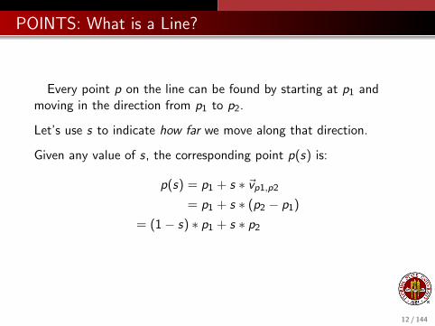
POINTS: What is a Line?
Every point p on the line can be found by starting at p1 andmoving in the direction from p1 to p2.
Let’s use s to indicate how far we move along that direction.
Given any value of s, the corresponding point p(s) is:
p(s) = p1 + s ∗ ~vp1,p2= p1 + s ∗ (p2 − p1)
= (1− s) ∗ p1 + s ∗ p2
12 / 144

POINTS: Examples
Choose p1 = (0,4), and p2 = (3,1). Then ~vp1,p2 = (3,-3).
s p1 + s * p2-p1 = p
--- ---- ---- ------ ---------
-1 (0,4) - 1 * (3,-3) = (-3, 7 )
0 (0,4) + 0 * (3,-3) = ( 0, 4 )
1/3 (0,4) + 1/3 * (3,-3) = ( 1, 3 )
1/2 (0,4) + 1/2 * (3,-3) = ( 1.5, 2.5)
2/3 (0,4) + 2/3 * (3,-3) = ( 2, 2 )
1 (0,4) + 1 * (3,-3) = ( 3, 1 )
2 (0,4) + 2 * (3,-3) = ( 6, -2 )
13 / 144
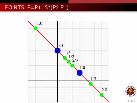
POINTS: P=P1+S*(P2-P1)
14 / 144

POINTS: Advantages of a Formula
Having this formula for a line is a huge advantage:
the formula can be regarded as the definition of the line;
we can compute points on a line;
we can solve for s given a desired x or y location;
we can guess how to define lines in 1D, 3D, or any dimension;
the value s is like a coordinate;
in any dimension, we only need 1 number to locate points.
We commonly refer to s as a parameter, a sort of index that allowsus to keep track of all the points on the line in an orderly way.
15 / 144

POINTS: The S Coordinate
The value of the s coordinate contains useful information:
It indicates that every line is really a one dimensional object,because its points can be indexed by a single number;
Points with 0 ≤ s ≤ 1 are between p1 and p2; if we restrictourselves to these points, we have a line segment;
Points with s < 0 or 1 < s are to the “left” or “right”;
If we know how far p2 is from p1, that is, ||p2− p1||, then smeasures the (signed) distance from p1 to the point p(s) inunits of that basic distance.
When we get to triangles, we will see a similar coordinate system.
16 / 144
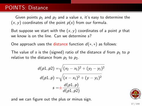
POINTS: Distance
Given points p1 and p2 and a value s, it’s easy to determine the(x , y) coordinates of the point p(s) from our formula.
But suppose we start with the (x , y) coordinates of a point p thatwe know is on the line. Can we determine s?
One approach uses the distance function d(∗, ∗) as follows:
The value of s is the (signed) ratio of the distance d from p1 to prelative to the distance from p1 to p2.
d(p1, p2) =√
(x2 − x1)2 + (y2 − y1)2
d(p1, p) =√
(x − x1)2 + (y − y1)2
s =± d(p1, p)
d(p1, p2)
and we can figure out the plus or minus sign.17 / 144
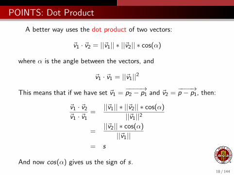
POINTS: Dot Product
A better way uses the dot product of two vectors:
~v1 · ~v2 = ||~v1|| ∗ ||~v2|| ∗ cos(α)
where α is the angle between the vectors, and
~v1 · ~v1 = ||~v1||2
This means that if we have set ~v1 =−−−−→p2 − p1 and ~v2 =
−−−−→p − p1, then:
~v1 · ~v2~v1 · ~v1
=||~v1|| ∗ ||~v2|| ∗ cos(α)
||~v1||2
=||~v2|| ∗ cos(α)
||~v1||= s
And now cos(α) gives us the sign of s.18 / 144

POINTS: Example
With p1 = (0, 4), and p2 = (3, 1), let p = (−2, 6).
Distance method:
d(p1, p2) =√
9 + 9 =√
18 = 3√
2.
d(p1, p) =√
4 + 4 =√
8 = 2√
2
s =± 2√
2
3√
2= −2
3
Dot product:
v1 =p2− p1 = (3,−3)
v2 =p − p1 = (−2, 2)
s =~v1 · ~v2~v1 · ~v1
=−6− 6
9 + 9= −12
18= −2
3
19 / 144
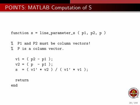
POINTS: MATLAB Computation of S
function s = line_parameter_s ( p1, p2, p )
% P1 and P2 must be column vectors!
% P is a column vector.
v1 = ( p2 - p1 );
v2 = ( p - p1 );
s = ( v1’ * v2 ) / ( v1’ * v1 );
return
end
20 / 144
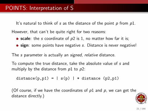
POINTS: Interpretation of S
It’s natural to think of s as the distance of the point p from p1.
However, that can’t be quite right for two reasons:
scale: the s coordinate of p2 is 1, no matter how far it is;
sign: some points have negative s. Distance is never negative!
The s parameter is actually an signed, relative distance.
To compute the true distance, take the absolute value of s andmultiply by the distance from p1 to p2:
distance(p,p1) = | s(p) | * distance (p2,p1)
(Of course, if we have the coordinates of p1 and p, we can get thedistance directly.)
21 / 144

POINTS: MATLAB Computation of S
This works fine if we type
p1 = [0;4]; p2 = [3;1]; p = [2;2];
s = line_parameter_s ( p1, p2, p );
but it will fail if we try to squeeze in several points at once!
p = [2,2; -3,7; 1.5,2.5; 6,-2]’;
??? Error using ==> minus
Matrix dimensions must agree.
Error in ==> line_parameter_s at 22
v2 = ( p - p1 );
But there’s no real reason the function can’t do all thesecalculations at once.
And MATLAB always encourages us to write programs that handledata in batches, rather than one data item at a time.
22 / 144
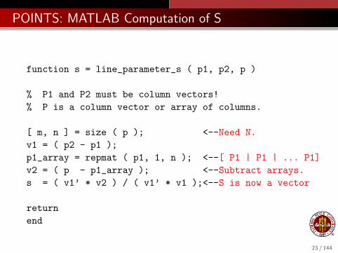
POINTS: MATLAB Computation of S
function s = line_parameter_s ( p1, p2, p )
% P1 and P2 must be column vectors!
% P is a column vector or array of columns.
[ m, n ] = size ( p ); <--Need N.
v1 = ( p2 - p1 );
p1_array = repmat ( p1, 1, n ); <--[ P1 | P1 | ... P1]
v2 = ( p - p1_array ); <--Subtract arrays.
s = ( v1’ * v2 ) / ( v1’ * v1 );<--S is now a vector
return
end
23 / 144
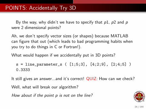
POINTS: Accidentally Try 3D
By the way, why didn’t we have to specify that p1, p2 and pwere 2 dimensional points?
Ah, we don’t specify vector sizes (or shapes) because MATLABcan figure that out (which leads to bad programming habits whenyou try to do things in C or Fortran!).
What would happen if we accidentally put in 3D points?
s = line_parameter_s ( [1;5;3], [4;2;9], [2;4;5] )
0.3333
It still gives an answer...and it’s correct! QUIZ: How can we check?
Well, what will break our algorithm?
How about if the point p is not on the line?
24 / 144

Geometry Algorithms
Overview
The Points on a Line
Points NOT on a Line
Estimating Integrals over an Interval
Triangles and their Properties
Triangulating a Polygon
The Convex Hull
Triangulating a Point Set by Delaunay
Estimating Integrals over a Triangle
Conclusion
25 / 144
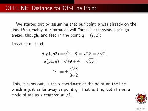
OFFLINE: Distance for Off-Line Point
We started out by assuming that our point p was already on theline. Presumably, our formulas will “break” otherwise. Let’s goahead, though, and feed in the point q = (7, 2):
Distance method:
d(p1, p2) =√
9 + 9 =√
18 = 3√
2.
d(p1, q) =√
49 + 4 =√
53 =
”s” =±√
53
3√
2
This, it turns out, is the s coordinate of the point on the linewhich is just as far away as point q. That is, they both lie on acircle of radius s centered at p1.
26 / 144

OFFLINE: Dot Product for Off-Line Point
Now let’s try the dot product:
v1 =p2− p1 = (3,−3)
v2 =q − p1 = (7,−2)
”s” =~v1 · ~v2~v1 · ~v1
=+21 + 6
9 + 9=
27
18=
3
2
This is much more interesting. It is the s coordinate of the pointon the line that is the nearest to q! That’s an interestinggeometric computation!
27 / 144

OFFLINE: Dot Product for Off-Line Point
28 / 144

OFFLINE: Distance from Point to Line
Using the dot product, we have been able to compute an scoordinate for all points in the plane, in a way that is very similarto Cartesian coordinates.
Now if we only know the s coordinate of a point, we still have a lotof points to choose from. It sure would be nice to have a tcoordinate that would answer that question. Now t should be zeroif the point is on the line, and I guess it should be 1 if the point is1 unit away, and so on.
So one way to go is to start with q, compute s, find thecorresponding nearest point p on the line, and then compute t asthe distance from p to q.
s = line_parameter_s ( p1, p2, q );
p = p1 + s * ( p2 - p1 );
t = norm ( p - q );
29 / 144

OFFLINE: A Perpendicular Axis
Now two vectors are perpendicular if their dot product is zero.
Given a (nonzero) 2D vector ~v = (vx , vy ), one vector that isperpendicular to ~v is ~w = (−vy ,+vx):
~v · ~w = vx ∗ wx + vy ∗ wy = −vx ∗ vy + vy ∗ vx = 0
Now let ~v be the unit direction vector of the line, that is,
~v = (p2− p1)/||p2− p1||
and use the formula to define a vector ~w perpendicular to ~v .Moreover, let’s normalize ~w to have unit length.
The two points on the line already defined the direction vector~v = p2− p1, which played the role of the x axis.
Now we have a perpendicular direction ~w , just like a y axis.
30 / 144

OFFLINE: Distance from Point to Line
A nonzero dot product equals the product of the vector lengthsand the cosine of the angle between them.
Let q be a point not on the line, and compute the dot product of~w with the direction vector
−−−→q − p:
~w · −−−−→q − p1 = ||w || ||q − p1|| cos(α) = ||q − p1|| cos(α) = t
If q is actually on the line, then t is zero. Otherwise, t is the(signed) length of the side of a right triangle with vertex p1,hypotenuse q − p1, and adjacent side that is part of the linethrough p1 and p2.
Our new S and T axes decompose the vector−−−→q − p into parallel
and perpendicular parts. They almost behave like x and y axes,except that we never properly scaled distances in the S direction.
So now, let us define a normalized coordinate s = s/||p2− p1||.31 / 144

OFFLINE: Distance of Point to Line
32 / 144
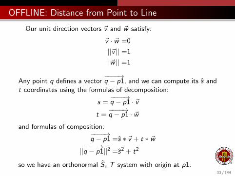
OFFLINE: Distance from Point to Line
Our unit direction vectors ~v and ~w satisfy:
~v · ~w =0
||~v || =1
||~w || =1
Any point q defines a vector−−−−→q − p1, and we can compute its s and
t coordinates using the formulas of decomposition:
s =−−−−→q − p1 · ~v
t =−−−−→q − p1 · ~w
and formulas of composition:−−−−→q − p1 =s ∗ ~v + t ∗ ~w
||−−−−→q − p1||2 =s2 + t2
so we have an orthonormal S , T system with origin at p1.33 / 144

OFFLINE: MATLAB Computation of T
function t = line_parameter_t ( p1, p2, p )
% P1, P2, P must be column vectors;
% The spatial dimension must be 2.
v1 = ( p2 - p1 );
v2 = ( p - p1 );
nv = [ -v1(2); v1(1) ];
nv = nv / norm ( nv );
t = nv’ * v2;
return
end
34 / 144
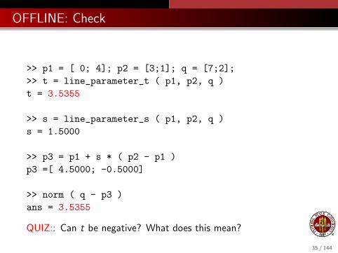
OFFLINE: Check
>> p1 = [ 0; 4]; p2 = [3;1]; q = [7;2];
>> t = line_parameter_t ( p1, p2, q )
t = 3.5355
>> s = line_parameter_s ( p1, p2, q )
s = 1.5000
>> p3 = p1 + s * ( p2 - p1 )
p3 =[ 4.5000; -0.5000]
>> norm ( q - p3 )
ans = 3.5355
QUIZ:: Can t be negative? What does this mean?
35 / 144
OFFLINE: A MATLAB Function
If the vector ~w is a unit normal vector, then so is −~w , and if wehad used that vector instead, all our t values would switch sign.
So the sign of the t parameter is arbitrary (we usually use the righthand rule to pick ~w). But whichever normal vector we choose, thesign of t divides all points into three classes: to the left of the line,on the line, or to the right.
It’s easy to make a simplified copy of line parameter t(p1,p2,p)called line side(p1,p2,p) returning:
+1 if p is to the left of the line;
0 if p is on the line;
-1 if p is to the right of the line.
Such an orientation function is handy when we look at triangles!
36 / 144

OFFLINE: Summary
We’ve run across some examples of classic geometric tasks:
parameterization: where is the point p on the line;
containment: is the point p on the line from p1 to p2?
distance: how far is the point q from the line?
nearness: which point p on the line is nearest the point q?
orientation: which side of the line is offline point q?
parameterization: where is the offline point q?
parallel and orthogonal: how we moved along the line, orsearched for nearest points.
mapping: we established a relationship between (x , y) and(s, t) coordinate systems.
37 / 144
OFFLINE: Summary
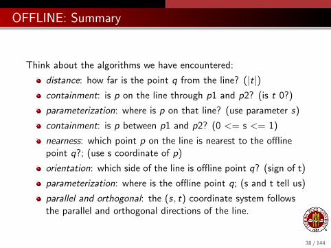
Think about the algorithms we have encountered:
distance: how far is the point q from the line? (|t|)containment: is p on the line through p1 and p2? (is t 0?)
parameterization: where is p on that line? (use parameter s)
containment: is p between p1 and p2? (0 <= s <= 1)
nearness: which point p on the line is nearest to the offlinepoint q?; (use s coordinate of p)
orientation: which side of the line is offline point q? (sign of t)
parameterization: where is the offline point q; (s and t tell us)
parallel and orthogonal: the (s, t) coordinate system followsthe parallel and orthogonal directions of the line.
38 / 144

Geometry Algorithms
Overview
The Points on a Line
Points NOT on a Line
Estimating Integrals over an Interval
Triangles and their Properties
Triangulating a Polygon
The Convex Hull
Triangulating a Point Set by Delaunay
Estimating Integrals over a Triangle
Conclusion
39 / 144

INTEGRALS: Random Samples
Monte Carlo algorithms work by sampling a set of data.
A Monte Carlo method for estimating the integral of a functionover the 1D interval p1 ≤ x ≤ p2 would need to pick pointsrandomly over this line segment.
Luckily, our way of describing a line as points p(s) fits thisperfectly. Not only do we have a formula for choosing points, butthe points between p1 and p2 are exactly those for which0 ≤ s ≤ 1. That means we can call our random number generatorand take its output to be the values of s that determine our points.
This works the same whether our interval is 1D, or for some reasonis a line in 2D or higher dimensions.
40 / 144
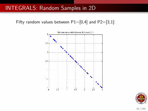
INTEGRALS: Random Samples in 2D
Fifty random values between P1=[0,4] and P2=[3,1]:
41 / 144
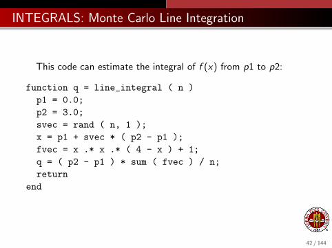
INTEGRALS: Monte Carlo Line Integration
This code can estimate the integral of f (x) from p1 to p2:
function q = line_integral ( n )
p1 = 0.0;
p2 = 3.0;
svec = rand ( n, 1 );
x = p1 + svec * ( p2 - p1 );
fvec = x .* x .* ( 4 - x ) + 1;
q = ( p2 - p1 ) * sum ( fvec ) / n;
return
end
42 / 144
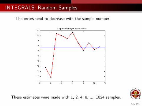
INTEGRALS: Random Samples
The errors tend to decrease with the sample number.
These estimates were made with 1, 2, 4, 8, ..., 1024 samples.
43 / 144

INTEGRALS: Random Samples
The trend is clearer for the absolute value of the error.
44 / 144
INTEGRALS: Random Samples
The Monte Carlo method works in part by being able to rapidlycompute uniform random sample points from the line segment[p1, p2].
It’s easy to compare Monte Carlo results with exact integration inthis case.
But when the region is a triangle, the interior of an ellipse, or thesurface of a sphere...or even a teapot, exact integration techniquesare not available. So ideas like the Monte Carlo sampling methodwill be extremely useful.
This has also been our first example of a computational algorithmthat involves sampling.
45 / 144
Geometry Algorithms
Overview
The Points on a Line
Points NOT on a Line
Estimating Integrals over an Interval
Triangles and their Properties
Triangulating a Polygon
The Convex Hull
Triangulating a Point Set by Delaunay
Estimating Integrals over a Triangle
Conclusion
46 / 144
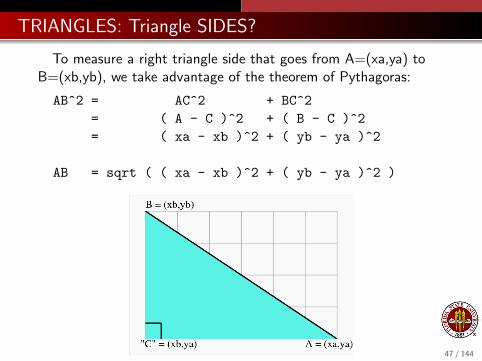
TRIANGLES: Triangle SIDES?
To measure a right triangle side that goes from A=(xa,ya) toB=(xb,yb), we take advantage of the theorem of Pythagoras:
AB^2 = AC^2 + BC^2
= ( A - C )^2 + ( B - C )^2
= ( xa - xb )^2 + ( yb - ya )^2
AB = sqrt ( ( xa - xb )^2 + ( yb - ya )^2 )
47 / 144
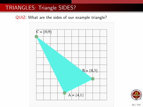
TRIANGLES: Triangle SIDES?
QUIZ: What are the sides of our example triangle?
48 / 144
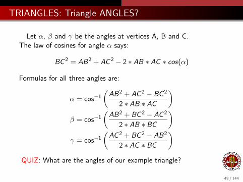
TRIANGLES: Triangle ANGLES?
Let α, β and γ be the angles at vertices A, B and C.The law of cosines for angle α says:
BC 2 = AB2 + AC 2 − 2 ∗ AB ∗ AC ∗ cos(α)
Formulas for all three angles are:
α = cos−1(
AB2 + AC 2 − BC 2
2 ∗ AB ∗ AC
)β = cos−1
(AB2 + BC 2 − AC 2
2 ∗ AB ∗ BC
)γ = cos−1
(AC 2 + BC 2 − AB2
2 ∗ AC ∗ BC
)QUIZ: What are the angles of our example triangle?
49 / 144
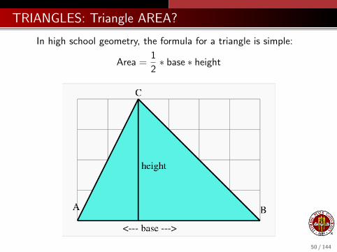
TRIANGLES: Triangle AREA?
In high school geometry, the formula for a triangle is simple:
Area =1
2∗ base ∗ height
50 / 144

TRIANGLES: Triangle AREA?
Such a formula doesn’t help when we don’t have a ruler and aprotractor, but rather a set of coordinates:
T = [ A, B, C ] = [ xa, xb, xc ] = [ 4, 8, 0 ]
[ ya, yb, yc ] [ 1, 3, 9 ]
51 / 144
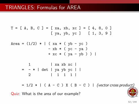
TRIANGLES: Formulas for AREA
T = [ A, B, C ] = [ xa, xb, xc ] = [ 4, 8, 0 ]
[ ya, yb, yc ] [ 1, 3, 9 ]
Area = (1/2) * | ( xa * ( yb - yc )
- xb * ( yc - ya )
+ xc * ( ya - yb ) ) |
1 | xa xb xc |
= - * | det | ya yb yc | |
2 | 1 1 1 |
= 1/2 * | ( A - C ) X ( B - C ) | (vector cross product)
Quiz: What is the area of our example?
52 / 144
TRIANGLES: Signs and Orientation
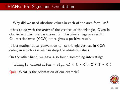
Why did we need absolute values in each of the area formulas?
It has to do with the order of the vertices of the triangle. Given inclockwise order, the basic area formulas give a negative result.Counterclockwise (CCW) order gives a positive result.
It is a mathematical convention to list triangle vertices in CCWorder, in which case we can drop the absolute values.
On the other hand, we have also found something interesting:
triangle orientation = sign of ( A - C ) X ( B - C )
Quiz: What is the orientation of our example?
53 / 144

TRIANGLES: Triangle CONTAINS Point?
We now come to a question that doesn’t seem to involve acomputation, namely, is a point P inside or outside of triangle T?
We can answer this question immediately if we draw a picture.However, we need to find a way of answering this question that isan algorithm, that is, computational and automatic.
If we can answer this question, we will have an idea how to answerthe same question in 3D (for a tetrahedron) and higher, abstractdimensions, where drawing a picture would be out of the question.
So even though we think our eye can answer this question, wedon’t want to have to use our eye to examine a million cases, or to“look” in 4D. A general algorithm will come in very handy!
54 / 144
TRIANGLES: A Walk Around the Block
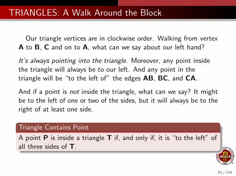
Our triangle vertices are in clockwise order. Walking from vertexA to B, C and on to A, what can we say about our left hand?
It’s always pointing into the triangle. Moreover, any point insidethe triangle will always be to our left. And any point in thetriangle will be “to the left of” the edges AB, BC, and CA.
And if a point is not inside the triangle, what can we say? It mightbe to the left of one or two of the sides, but it will always be to theright of at least one side.
Triangle Contains Point
A point P is inside a triangle T if, and only if, it is “to the left” ofall three sides of T.
55 / 144
TRIANGLES: A MATLAB Function
Recall our function for the location of a point relative to a line.
The value returned by line side(A,B,P) is:
+1 if P is to the left of the line through AB;
0 if P is on the line through AB;
-1 if P is to the right of the line through AB.
Suppose we call this function three times, to check the status of Pwith respect to the lines through the segments AB, BC and CA!
56 / 144

TRIANGLES: QUIZ
Interpret these results:
AB BC CA Meaning?
P1 +1 +1 +1
P2 -1 +1 +1
P3 +1 -1 +1
P4 +1 +1 -1
P5 +1 -1 -1
P6 -1 +1 -1
P7 -1 +1 +1
P8 -1 -1 -1
There is something a little odd about one result.57 / 144
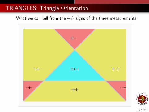
TRIANGLES: Triangle Orientation
What we can tell from the +/- signs of the three measurements:
58 / 144

TRIANGLES: We could also check for zero values
AB BC CA Meaning?
P9 0 +1 +1 inside, but on side AB
P10 +1 0 +1 inside, but on side BC
P11 +1 +1 0 inside, but on side CA
P12 +1 0 0 what is this?
P13 0 +1 0
P14 0 0 +1
P15 0 +1 -1 where is this?
...
P21 -1 0 0 why can’t this happen?
...
P27 0 0 0 how could this be possible?
59 / 144

TRIANGLES: Triangle Orientation
What we can tell if we include 0:
60 / 144
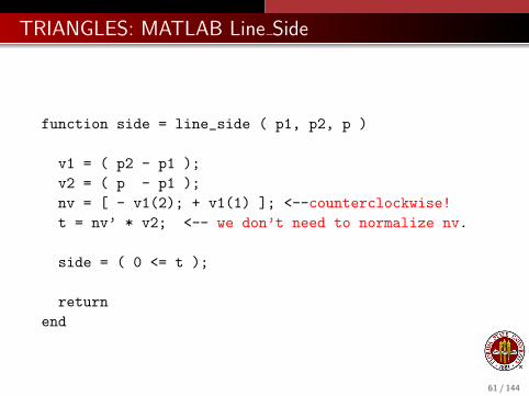
TRIANGLES: MATLAB Line Side
function side = line_side ( p1, p2, p )
v1 = ( p2 - p1 );
v2 = ( p - p1 );
nv = [ - v1(2); + v1(1) ]; <--counterclockwise!
t = nv’ * v2; <-- we don’t need to normalize nv.
side = ( 0 <= t );
return
end
61 / 144
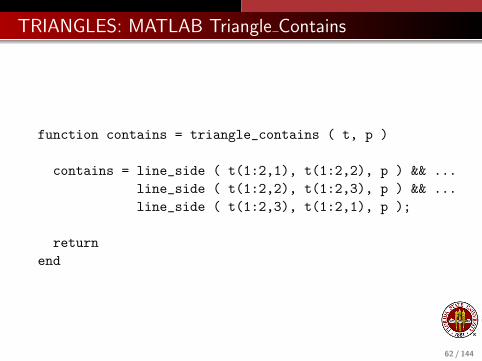
TRIANGLES: MATLAB Triangle Contains
function contains = triangle_contains ( t, p )
contains = line_side ( t(1:2,1), t(1:2,2), p ) && ...
line_side ( t(1:2,2), t(1:2,3), p ) && ...
line_side ( t(1:2,3), t(1:2,1), p );
return
end
62 / 144

TRIANGLES: Test Triangle Contains
function triangle contains test ( )
t = [ 4, 0; 3, 4; 0, 1 ]’;
p = [ 1, 4; 2, 1; 2, 3; 3, 2; 3, 4; 3, 5; 4, 1; 4, 5 ]’;
for j = 1 : 8
c = triangle_contains ( t, p(1:2,j) );
fprintf ( 1, ’ %10f %10f %2d\n’, p(1:2,j), c );
end
return
end
63 / 144
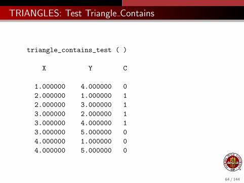
TRIANGLES: Test Triangle Contains
triangle_contains_test ( )
X Y C
1.000000 4.000000 0
2.000000 1.000000 1
2.000000 3.000000 1
3.000000 2.000000 1
3.000000 4.000000 1
3.000000 5.000000 0
4.000000 1.000000 0
4.000000 5.000000 0
64 / 144
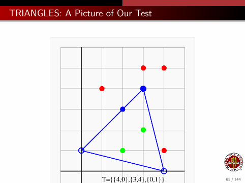
TRIANGLES: A Picture of Our Test
65 / 144
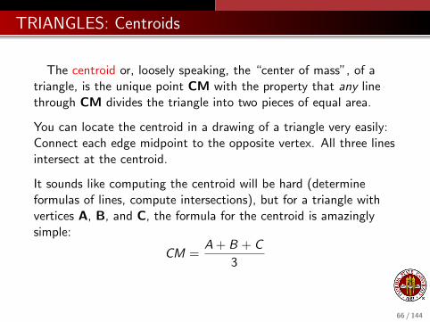
TRIANGLES: Centroids
The centroid or, loosely speaking, the “center of mass”, of atriangle, is the unique point CM with the property that any linethrough CM divides the triangle into two pieces of equal area.
You can locate the centroid in a drawing of a triangle very easily:Connect each edge midpoint to the opposite vertex. All three linesintersect at the centroid.
It sounds like computing the centroid will be hard (determineformulas of lines, compute intersections), but for a triangle withvertices A, B, and C, the formula for the centroid is amazinglysimple:
CM =A + B + C
3
66 / 144
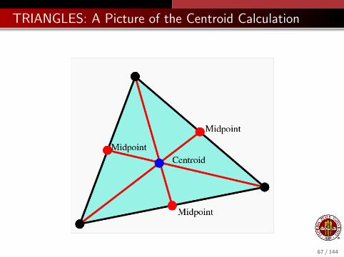
TRIANGLES: A Picture of the Centroid Calculation
67 / 144
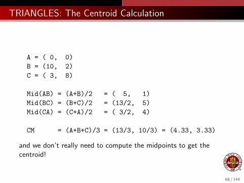
TRIANGLES: The Centroid Calculation
A = ( 0, 0)
B = (10, 2)
C = ( 3, 8)
Mid(AB) = (A+B)/2 = ( 5, 1)
Mid(BC) = (B+C)/2 = (13/2, 5)
Mid(CA) = (C+A)/2 = ( 3/2, 4)
CM = (A+B+C)/3 = (13/3, 10/3) = (4.33, 3.33)
and we don’t really need to compute the midpoints to get thecentroid!
68 / 144
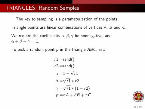
TRIANGLES: Random Samples
The key to sampling is a parameterization of the points.
Triangle points are linear combinations of vertices A, B and C .
We require the coefficients α, β, γ be nonnegative, andα + β + γ = 1.
To pick a random point p in the triangle ABC , set:
r1 =rand();
r2 =rand();
α =1−√
r1
β =√
r1 ∗ r2
γ =√
r1 ∗ (1− r2)
p =αA + βB + γC
69 / 144

TRIANGLES: Distance
For our last “trick” with triangles, let’s ask the simple question,how far is a point p from a triangle?
To answer this question, we begin by computing the quantitiessAB, tAB, sBC, tBC, xCA and tCA, the s and t parameters forthe point relative to the lines AB, BC , and CA.
If all three t parameters are nonnegative, the point is in or on thetriangle, and so the distance is zero.
If just one value of t is negative, then the nearest point is on theline, but the triangle includes just a segment of that line. If thecorresponding value of s is between 0 and 1, then the nearest pointis part of the line segment, and the distance is |t|. But if s < 0,the nearest point is the first vertex, and if 1 < s, the nearest pointis the second.
70 / 144
TRIANGLES: Distance
The last possibility is that two values of t are negative.
This means that the nearest point is on one of the two sides, ortheir common vertex.
We work by checking the two s values.
If both s values are “out of range” (that is, outside of [0,1]), thenthe vertex is the closest point.
If just one s value is in range, then the corresponding side is theclosest, so the distance is the corresponding value of |t|.
And it cannot be the case that both s values are in range.
71 / 144
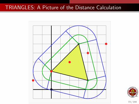
TRIANGLES: A Picture of the Distance Calculation
72 / 144

TRIANGLES: Summary of Algorithms
We have seen many triangle algorithms:
triangle angles();
triangle area();
triangle centroid();
triangle contains point();
triangle distance to point();
triangle orientation();
triangle perimeter(), (You can figure this one out!);
triangle sample();
triangle side lengths();
Many of these are building blocks for more complicated problems.
73 / 144
Geometry Algorithms
Overview
The Points on a Line
Points NOT on a Line
Estimating Integrals over an Interval
Triangles and their Properties
Triangulating a Polygon
The Convex Hull
Triangulating a Point Set by Delaunay
Estimating Integrals over a Triangle
Conclusion
74 / 144
POLYGONS: Let’s Not Start Over!
Triangles are the simplest of the polygons, which includesquares, pentagons, hexagons, and so on.
Unlike triangles, however polygons with 3 < N vertices:
are “bendable”; knowing the sides doesn’t tell us the shape.
might not be convex; there may be “bites” in the shape.
can cross edges, if we allow “misbehaving” (we won’t!);
However, every well-behaved polygon of N sides can betriangulated, that is, it can be decomposed into N-2 triangles,simply by drawing N-3 non-intersecting “diagonals”, that is, byconnecting pairs of vertices of the polygon.
75 / 144

POLYGONS: A Polygon with 18 Vertices
There are many ways to triangulate this polygon.They all end up with 16 triangles!
76 / 144
POLYGONS: Definition of CONVEX
I used the word convex a moment ago, and it will come up againfrom time to time.
In the plane, a convex polygon is one that has no “dents”.
The strict definition: The object C is convex if and only if,whenever two points p1 and p2 are elements of the object, so isevery point p that lies on the line segment between p1 and p2:
p = t ∗ p1 + (1− t) ∗ p2
0 ≤ t ≤ 1.
Circles, squares, regular pentagons are examples of convex shapes.
A star is not convex, nor are the letters of the alphabet, with thepossible exception of lowercase l and uppercase I when drawn in asans serif font!
77 / 144

POLYGONS: Let’s Not Start Over!
Rather than try to come up with new formulas for the analysis ofpolygons, it makes sense to triangulate a polygon, apply ourformulas to the triangles, and then figure out how to put togetherthose results to say something about the original polygon.
If we can determine a triangulation of a polygon, then
the area is the sum of the triangle areas;
a point is in the polygon if it is in a triangle;
the distance to the polygon is the minimum of the distancesto any triangle;
the centroid of the polygon is computable;
78 / 144

POLYGONS: A ”Snake” Polygon
79 / 144

POLYGONS: A Triangulated ”Snake” Polygon
80 / 144

POLYGONS: Ideas for Triangulation
Once again, it’s easy to see how to do something, but really hardto create an algorithm that works.
One approach starts with the idea of “Decrease and Conquer”;that is, we replace the original problem with a partial answer and asmaller problem.
Imagine the polygon was a kind of cake (with lots of corners!).Shouldn’t it always be possible to slice one triangular piece off?Doesn’t that reduce the number of vertices by one?
QUIZ: May there be some vertices we can’t immediately eliminate?Must there always be at least one that we can?
If the polygon is convex, can we cut off any slice (vertex) we like?
81 / 144

POLYGONS: Polygons Have Ears
An ear of a polygon is a triangle that can be formed by threeconsecutive vertices of the polygon in such a way that two edges ofthe triangle are edges of the polygon, and the third edge iscompletely contained inside the polygon.
An ear can be sliced off a polygon, reducing the vertices by 1.
We have the following very useful theorem:
If P is a simple polygon (no internal holes and no edge crossings)with at least 4 vertices, then P is guaranteed to have at least twodistinct ears. [Meisters, 1975]
Moreover if P is convex, every 3 consecutive vertices form an ear.
Can you spot the ears on our “snake” polygon?
82 / 144

POLYGONS: Ear Slicing
The ear theorem means that every polygon can be triangulated.
We start with a polygon of N vertices, and 0 diagonals.We locate an ear, defined by the consecutive vertices B, C, D.
We add the diagonal from B to D to our list.
We also remove C from the polygon, and decrease N by 1.
Now we have a polygon of N-1 vertices, and 1 diagonal.If N is still greater than 3, we repeat the process.
After slicing off N-3 ears, we have 3 vertices left, forming a singletriangle, which is our last ear.
Thus we end up with N-2 triangles by creating N-3 internaldiagonal lines.
The list of diagonals is our triangulation of the original polygon.
83 / 144
POLYGONS: Ear Detection
We need to be clear about the “find an ear” step!
Suppose we have vertices A, B, C, D and E, which are consecutivein the counterclockwise ordering. Then B, C and D form an ear if:
triangle BCD has positive area (= counterclockwise );
the (open) line segment BD doesn’t intersect any edge;
the line segment BD is “between” BA and BC;
the line segment DB is “between” DC and DE.
84 / 144

POLYGONS: Representing a Polygon
We represent a polygon as a linked list. We can delete anyvertex so that the remaining data represents the simplified polygon.
We must set up an array of things of vertex type.
Each vertex has fields called index, next, and prev.
We might store the polygon 1→ 2→ 3→ 4→ 1 by:
mypolygon
prev index next ear x y
4 1 2 1 0.0 0.0
1 2 3 1 1.0 0.0
2 3 4 1 1.0 1.0
3 4 1 1 0.0 1.0
Here the ear field is 1 if the vertex defines an ear.
85 / 144

POLYGONS: Removing an Ear
If we decide to remove the ear represented by vertices 2, 3 and4, then we must remove vertex 3 from the polygon so we have1→ 2→ 4→ 1 remaining.
Essentially, all we need to do is change the pointers:
mypolygon
prev index next ear x y
4 1 2 1 0.0 0.0
1 2 4 1 1.0 0.0
0 0 0 0 1.0 1.0
2 4 1 1 0.0 1.0
And now suddenly we have a triangle rather than a square!
86 / 144

POLYGONS: The Ear Removal Tasks
If we have decided that B, C and D form an ear then we need to
add diagonal B, D to our list;
remove vertex C from the polygon (reset C.index to 0);
reset B.next to D and D.prev to B;
reset B.ear if A, B, D has become an ear;
reset D.ear if B, D, C has become an ear.
87 / 144

POLYGONS: The Slicing Code
i2 = first;
while ( diagonal_num < n - 3 )
if ( vertex(i2).ear )
i3 = vertex(i2).next; i4 = vertex(i3).next;
i1 = vertex(i2).prev; i0 = vertex(i1).prev;
vertex(i1).next = i3;
vertex(i2).index = 0;
vertex(i3).prev = i1;
vertex(i1).ear = diagonal ( i0, i3, vertex );
vertex(i3).ear = diagonal ( i1, i4, vertex );
diagonal_num = diagonal_num + 1;
diagonals(diagonal_num,1) = i1;
diagonals(diagonal_num,2) = i3;
end
i2 = vertex(i2).next;
end 88 / 144
POLYGONS: An Example Implementation
An example of a MATLAB code for carrying out the ear-slicingalgorithm for polygon triangulation is available at:
http://people.sc.fsu.edu/∼jburkardt/m src/triangulate/triangulate.html
and a C version is available at
http://people.sc.fsu.edu/∼jburkardt/c src/triangulate/triangulate.html
89 / 144
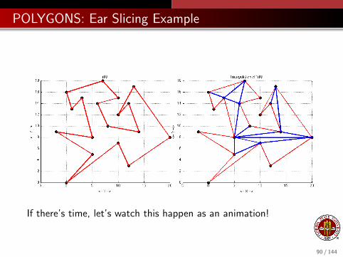
POLYGONS: Ear Slicing Example
If there’s time, let’s watch this happen as an animation!
90 / 144
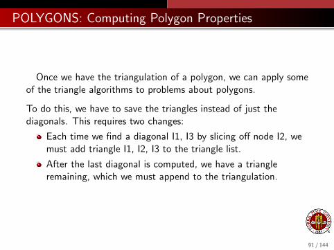
POLYGONS: Computing Polygon Properties
Once we have the triangulation of a polygon, we can apply someof the triangle algorithms to problems about polygons.
To do this, we have to save the triangles instead of just thediagonals. This requires two changes:
Each time we find a diagonal I1, I3 by slicing off node I2, wemust add triangle I1, I2, I3 to the triangle list.
After the last diagonal is computed, we have a triangleremaining, which we must append to the triangulation.
91 / 144
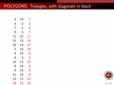
POLYGONS: Triangles, with diagonals in black
2 18 1
4 2 3
7 5 6
8 5 7
12 10 11
15 13 14
18 16 17
2 16 18
4 16 2
8 4 5
15 12 13
8 16 4
9 16 8
10 16 9
15 10 12
16 10 15 92 / 144

POLYGONS: Computing Polygon Properties
Some polygon algorithms don’t require a triangulation.
The side lengths can be computed simply by taking the norm ofthe vector from one vertex to the next.
The perimeter is just the sum of the side lengths.
The angles can be computed in a straightforward manner. If wehave consecutive vertices A, B, and C, then recall the formula
v1× v2 =||v1|| · ||v2|| · sin(θ)
v1 · v2 =||v1|| · ||v2|| · cos(θ)
θ =atan2(v1× v2, v1 · v2)
Letting v1 = (C − B) and v2 = (A− B), the formula gives theangle at vertex B.
93 / 144

POLYGONS: Computing Polygon Properties
The triangles making up a polygon can be used to computesome geometric quantities:
1 the area of the polygon is the sum of the areas of thetriangles;
2 the centroid of the polygon can be computed as the sum ofthe triangle centroids, each multiplied by its area, and thendivided by the total area;
3 a polygon contains a point if and only if one of the trianglescontains the point;
4 the distance from a point to a polygon is the minimum ofthe distances to the triangles;
94 / 144
POLYGONS: Random sampling
Can our triangle algorithms do random sampling of a polygon?
If we have triangulated the polygon, we can sample the polygon bysampling one of the triangles.
If one triangle has twice the area of another, then we shouldprobably sample it twice as often.
So the correct procedure is as follows:
1 let A(I) be the area of the I-th triangle, and ATOTAL thetotal area;
2 choose a random value r1, and consider B = r1 ∗ ATOTAL;
3 Using no triangles, we have 0 area, and using them all wehave ATOTAL; therefore, there is some triangle J so that thesum of areas 1 to J just reaches or exceeds B.
4 pick a random point from that triangle J;
95 / 144
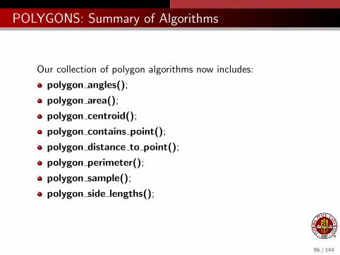
POLYGONS: Summary of Algorithms
Our collection of polygon algorithms now includes:
polygon angles();
polygon area();
polygon centroid();
polygon contains point();
polygon distance to point();
polygon perimeter();
polygon sample();
polygon side lengths();
96 / 144

Geometry Algorithms
Overview
The Points on a Line
Points NOT on a Line
Estimating Integrals over an Interval
Triangles and their Properties
Triangulating a Polygon
The Convex Hull
Triangulating a Point Set by Delaunay
Estimating Integrals over a Triangle
Conclusion
97 / 144
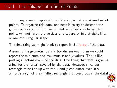
HULL: The “Shape” of a Set of Points
In many scientific applications, data is given at a scattered set ofpoints. To organize this data, one need is to try to describe thegeometric location of the points. Unless we are very lucky, thepoints will not lie on the vertices of a square, or in a straight line,or any other regular shape.
The first thing we might think to report is the range of the data.
Assuming the geometric data is two dimensional, then we couldreport the minimum and maximum x and y values. This is likeputting a rectangle around the data. One thing that does is give usa feel for the “area” covered by the data. However, since ourrectangle must line up with the x and y coordinate axes, it’salmost surely not the smallest rectangle that could box in the data!
98 / 144
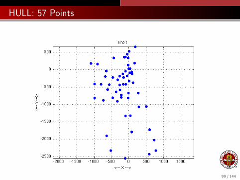
HULL: 57 Points
99 / 144

HULL
So we could imagine that we’re trying to fence in the data usinga rectangle that we can turn at an angle. If we’re paying for thefence, we’d like to use the least length possible.
What if we allowed ourselves to use pentagons instead? Theminimum fence length (the perimeter) over all possible pentagonsmust be as low, or lower, than what we can get with rectangles.
To drive the perimeter length as low as possible, we shouldconsider every possible polygon that encloses the data.
It’s clear that the “fence posts” will always occur at data points.
It should also be clear that the smallest perimeter requirementimplies that the hull will be convex.
The convex hull problem: find the convex polygon of smallestperimeter which contains a given set of points.
100 / 144

HULL: 57 Points Fenced In
101 / 144

HULL: Things to Note
The convex hull of this data was computed by MATLAB’sconvhull command.
The convex hull of a finite set of points is a polygon: every vertexis a data point, and every edge is a straight line segment.
In fact, if you had to build the cheapest fence that contained thedata, the bends in the fence would come at data points, just as wesee in the picture.
Looking at the picture, you can also imagine it to be a kind of“wrapping” problem, that is, we could imagine a group of treesthat we are going to surround with a rope fence. When we pull therope as tight as possible, we get the convex hull.
In fact, the idea of wrapping the data will lead us to an algorithm.
102 / 144

HULL: Convexity
Although polygons are allowed to have dents or wiggles, the convexhull of our data has no “dents” (and no internal holes either).
Quiz: Can you explain why this should be true?
The hull is called convex because if p and q are any points in theshape, so is every point on the line between p and q.
Although a convex shape can be described by its boundary, itactually is not just the boundary, but all points contained inside.
Thus, the letter “I is a convex shape, the letter “O” is not, but itis the boundary of a convex shape, while the letter “A” is neither aconvex shape nor the boundary of one.
103 / 144
HULL: Convexity
A second way to define the convex hull of a set of points is thatit is the smallest convex shape that contains the points.
If a shape is convex, it is its own convex hull (this must be true!)
But wait a minute...a circle is convex, so it’s a convex hull. But wesaid a minute ago that the convex hull is a polygon, made withstraight line segments. Is there a contradiction here?
The definitions of a convex shape and a convex hull can beextended to higher dimensions.
104 / 144

HULL: Not just geometry!
Like many things in mathematics, the convex hull is not simply aquestion about geometry!
We often have cases where we have a great deal of data available,which we think of as samples from some larger set of possibilities.
One way to sample that larger set begins by constructing theconvex hull of the data. The convex hull is a polygon, so we cantriangulate it, and hence take sample values. By sampling withinthe convex hull, our “simulated” data stays within the range of theoriginal data, but can return completely new values within thatrange.
105 / 144

HULL: A data hull for sampling
106 / 144

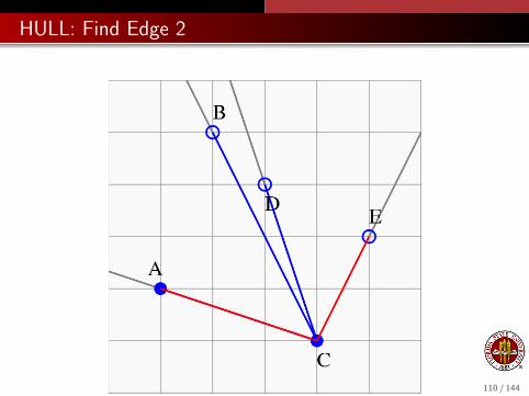
HULL: The Wrapping Algorithm
We can always find one point on the convex hull: simply find thepoint with the minimum x component. If there are several pointswith the same minimal x component, choose the one with smallesty component. That gets us started, with a data point we will callvertex H1.
Now we have to determine the next vertex of the polygon. Wehave N-1 datapoints to choose from. Let’s assume we are trying tobuild the polygon by following the vertices in the counterclockwisedirection. So we have N-1 possible edges, from H1 to each of theunused datapoints.
The correct edge (H1,H2) is the unique line through H1 to somevertex V with the property that all data points lie to the left of it.
107 / 144
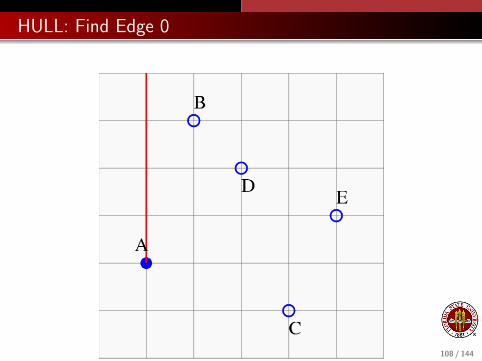
HULL: Find Edge 0
108 / 144

HULL: Find Edge 1
109 / 144
HULL: Find Edge 2
110 / 144
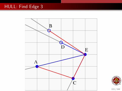
HULL: Find Edge 3
111 / 144
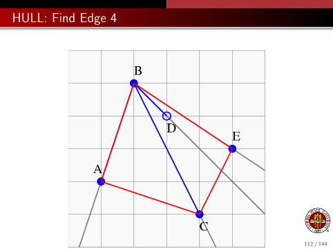
HULL: Find Edge 4
112 / 144

HULL: Finished
113 / 144

HULL; Summary
For a convex hull calculation in MATLAB, use a command like
k = convhull ( x, y )
k indexes the points which form the convex hull. From k we havethe polygon containing the points, hence the area, the perimeter,the ability to sample, and so on.
To see a plot of the data points and their hull, use:
plot ( x, y, ’.’ );k = convhull ( x, y )hold onplot ( x(k), y(k), ’-r’ )hold off
The command convhulln() is available for higher dimensions.
114 / 144
Geometry Algorithms
Overview
The Points on a Line
Points NOT on a Line
Estimating Integrals over an Interval
Triangles and their Properties
Triangulating a Polygon
The Convex Hull
Triangulating a Point Set by Delaunay
Estimating Integrals over a Triangle
Conclusion
115 / 144
DELAUNAY: The Point Set Problem
Suppose we draw a number of points on the plane. It is certainlypossible to draw a line connecting two of the points. Now let’sdraw another line...except that we are not allowed to cross the firstline. That should still be easy. Surely we can draw many lines, butjust as surely, there will come a point when we cannot draw anymore lines without crossing one we already drew.
It may surprise you to realize that, for a given set of points, thereare many final results possible, but in every case, if we cannot drawany more lines, then all the points on the plane are now vertices oftriangles.
We have now triangulated a set of points. This is similar to theproblem of triangulating a polygon, but now we do not start with abounding polygon, and we imagine we might have many points dodeal with, so efficiency is important.
116 / 144
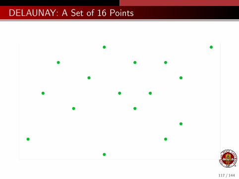
DELAUNAY: A Set of 16 Points
117 / 144
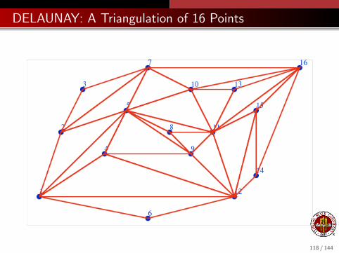
DELAUNAY: A Triangulation of 16 Points
118 / 144
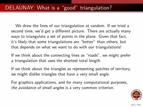
DELAUNAY: What is a “good” triangulation?
We drew the lines of our triangulation at random. If we tried asecond time, we’d get a different picture. There are actually manyways to triangulate a set of points in the plane. Given that fact,it’s likely that some triangulations are “better” than others, butthat depends on what we want to do with our triangulations!
If we think about the connecting lines as “roads”, we might prefera triangulation that uses the shortest total length.
If we think about the triangles as representing patches of territory,we might dislike triangles that have a very small angle.
For graphics applications, and for many computational purposes,the avoidance of small angles is a very common criterion.
119 / 144

DELAUNAY: What is a “good” triangulation?
The Delaunay triangulation of a set of points is the (usuallyunique) triangulation which does the best job of avoiding smallangles.
More strictly speaking, consider all possible triangulations of a setof data points. For each triangulation T , let θ(T ) be the smallestangle that occurs in any triangle of that triangulation. Then atriangulation T ∗ is a Delaunay triangulation if
θ(T ) ≤ θ(T ∗)
for all triangulations T .
120 / 144

DELAUNAY: A Triangulation of 16 Points
121 / 144
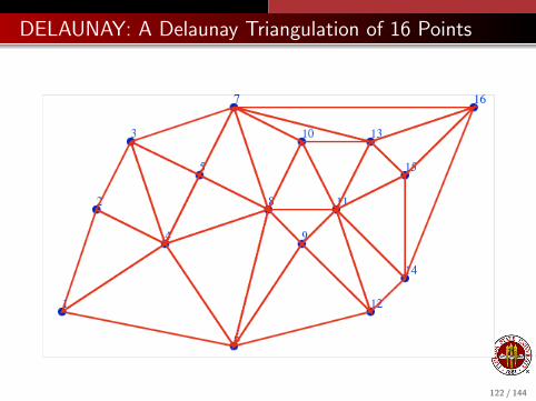
DELAUNAY: A Delaunay Triangulation of 16 Points
122 / 144

DELAUNAY: MATLAB Calculation
To compute the triangles that form a Delaunay triangulation ofa set of data points, use the MATLAB command
tri = delaunay ( x, y )
To display the triangulation,
tri = delaunay ( x, y )triplot ( tri, x, y )
123 / 144

DELAUNAY: 3D Surfaces
Often, measurements of a 3D surface are available at an irregularlyscattered set of points.
If we can organize the (X,Y) data into a triangular mesh, then overeach triangle, we can draw a flat surface defined by the threecorresponding Z values.
Doing this for each triangle in the mesh, we can create a 3D imageof the surface, where before we simply had point data.
load seamount (...a built in XYZ dataset)tri = delaunay ( x, y )trisurf ( tri, x, y, z )
124 / 144

DELAUNAY: A 3D Image from XYZ Point Data
125 / 144
Geometry Algorithms
Overview
The Points on a Line
Points NOT on a Line
Estimating Integrals over an Interval
Triangles and their Properties
Triangulating a Polygon
The Convex Hull
Triangulating a Point Set by Delaunay
Estimating Integrals over a Triangle
Conclusion
126 / 144
INTEGRALS: Now the Region is the Problem!
When you learned integration in Calculus, you probably beganwith the idea that it was simply “the inverse” of differentiation.Why someone would want to differentiate a formula and thenintegrate it back was not clear.
Perhaps later you were told a much more suggestive interpretationof integration: integration carries out the summation of “verymany” “very small” terms.
Thus, we approximated the integral of a function (the area underits curve) by a sum over many subintervals, with the true integralbeing the limit as these subintervals become arbitrarily small.
We saw many unusual functions to integrate, but the integrationregion itself was usually simple: an interval, or perhaps a box, orvery occasionally a surface of rotation...which turned out to be justan interval plus a “twist”.
127 / 144

INTEGRALS: Simple Function, Weird Geometry!
Real life problems require us to use Calculus in new ways.
Computing the area of this hand is the same as integratingf (x , y) = 1. The difficulties come not from the function, but theunusual region.
128 / 144
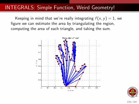
INTEGRALS: Simple Function, Weird Geometry!
Keeping in mind that we’re really integrating f (x , y) = 1, wefigure we can estimate the area by triangulating the region,computing the area of each triangle, and taking the sum.
129 / 144

INTEGRALS: Integrating F(X,Y)=1 is Easy
But now suppose that I wanted to compute the volume of thishand, and that for any point (x , y) I can measure the height orthickness of the hand, which I can regard as the function f (x , y).
Volume =
∫hand
f (x , y)dx dy
An accurate estimate of this integral will approximate the volumeof the hand.
I knew how to integrate the function f (x , y) = 1, because that wasjust the area. But now I have an integral of a complicated functionf (x , y) over a complicated region.
What do I do?
130 / 144

INTEGRALS: Approximate Integration over Triangles
When we computed the area, we broke the region up intotriangles. That idea is still the right way to go, because it reducesthe complicated geometry to a sum of simple geometries.
We are left with the problem of approximating the integral of afunction over a general triangle.
For special cases where the triangle has two sides aligned with thex and y axes, we can come up with exact integration formulas.But for the hand volume problem, this is not realistic to expect.
Instead, we will turn to some very useful formulas which allow usto estimate the integral of a function over any triangle as aweighted average of its value at a few prescribed points.
This technique is known as quadrature.
131 / 144
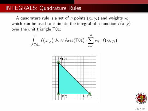
INTEGRALS: Quadrature Rules
A quadrature rule is a set of n points (xi , yi ) and weights wi
which can be used to estimate the integral of a function f (x , y)over the unit triangle T01:∫
T01f (x , y) dx ≈ Area(T01) ·
n∑i=1
wi · f (xi , yi )
132 / 144

INTEGRALS: A Rule of Precision 1
By averaging the function value at the vertices, we get a rulewhich approximate the integral, and is actually exactly right iff (x , y) is equal to a constant, or a linear function.
Points: Weights:
------------------------ ------------------------
x = [ 1, 0, 0 ]; w = [ 1/3, 1/3, 1/3 ];
y = [ 0, 1, 0 ];
133 / 144

INTEGRALS: A Rule of Precision 1
Another nice thing about the vertex rule is that it’s obvious howto use the same rule on a general triangle.
Since the vertex rule is only “precise” for constants and linears, itis natural to seek rules that are “more precise”, that is, which getthe exact answer when the function is any polynomial up to somegiven degree.
Using just 6 function values, we can devise a rule through degree4, so that it can integrate exactly any polynomial like:
f (x , y) =a
+bx + cy
+dx2 + exy + fy2
+gx3 + hx2y + ixy2 + jy3
+kx4 + lxy3 + mx2y2 + nxy3 + oy4
134 / 144

INTEGRALS: A Rule of Precision 4
Points: Weights:
------------------------ ------------------------
a = 0.816847572980459;
b = 0.091576213509771;
c = 0.108103018168070; u = 0.109951743655322;
d = 0.445948490915965; v = 0.223381589678011;
x = [ a, b, b, c, d, d ]; w = [ u, u, u, v, v, v ];
y = [ b, a, b, d, c, d ];
135 / 144
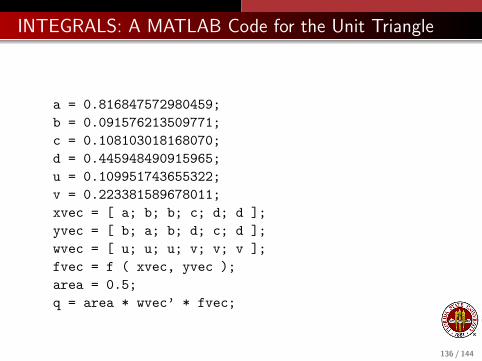
INTEGRALS: A MATLAB Code for the Unit Triangle
a = 0.816847572980459;
b = 0.091576213509771;
c = 0.108103018168070;
d = 0.445948490915965;
u = 0.109951743655322;
v = 0.223381589678011;
xvec = [ a; b; b; c; d; d ];
yvec = [ b; a; b; d; c; d ];
wvec = [ u; u; u; v; v; v ];
fvec = f ( xvec, yvec );
area = 0.5;
q = area * wvec’ * fvec;
136 / 144

INTEGRALS: A Rule of Precision 4
Here is a plot of the quadrature points as they are arranged inthe unit triangle T01.
This means we can now approximate integrals over the unittriangle, but what do we do for integrals over an arbitrary triangleABC, which is what we actually need?
137 / 144
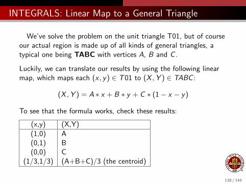
INTEGRALS: Linear Map to a General Triangle
We’ve solve the problem on the unit triangle T01, but of courseour actual region is made up of all kinds of general triangles, atypical one being TABC with vertices A, B and C .
Luckily, we can translate our results by using the following linearmap, which maps each (x , y) ∈ T 01 to (X ,Y ) ∈ TABC :
(X ,Y ) = A ∗ x + B ∗ y + C ∗ (1− x − y)
To see that the formula works, check these results:
(x,y) (X,Y)
(1,0) A(0,1) B(0,0) C
(1/3,1/3) (A+B+C)/3 (the centroid)
138 / 144

INTEGRALS: A MATLAB Code for the General Triangle
A = [ ax; ay ];
B = [ bx; by ];
C = [ cx; cy ];
Xvec = ax * xvec + bx * yvec + cx * ( 1 - xvec - yvec );
Yvec = ay * xvec + by * yvec + cy * ( 1 - xvec - yvec );
Fvec = f ( Xvec, Yvec );
Area = triangle_area ( A, B, C );
q = Area * wvec’ * Fvec;
139 / 144
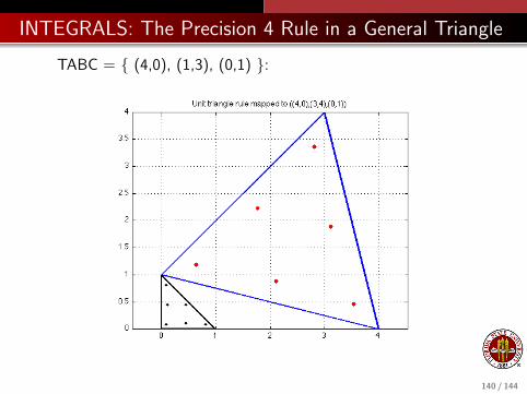
INTEGRALS: The Precision 4 Rule in a General Triangle
TABC = { (4,0), (1,3), (0,1) }:
140 / 144

Geometry Algorithms
Overview
The Points on a Line
Points NOT on a Line
Estimating Integrals over an Interval
Triangles and their Properties
Triangulating a Polygon
The Convex Hull
Triangulating a Point Set by Delaunay
Estimating Integrals over a Triangle
Conclusion
141 / 144

CONCLUSION: We’ve Shown You the Mountains
We have come a long, long way this semester, though we’ve onlyguided you to the the foothills of many interesting mountains.
142 / 144
CONCLUSION: Remember Some of those Mountains!
143 / 144

CONCLUSION: The Summit is Up to You
We hope the knowledge and tools we’ve shown you will enableyou to climb the mountains you choose to challenge!
144 / 144
Related Documents