Geometric Monitoring of Heterogeneous Streams (Long Version, with Proofs of the Theorems) Daniel Keren 1 , Guy Sagy 2 , Amir Abboud 2 , David Ben-David 2 , Assaf Schuster 2 , Izchak Sharfman 2 and Antonios Deligiannakis 3 1 Department of Computer Science, Haifa University 2 Faculty of Computer Science, Israeli Institute of Technology 3 Department of Electronic and Computer Engineering, Technical University of Crete Abstract Interest in stream monitoring is shifting toward the distributed case. In many applica- tions the data is high volume, dynamic, and distributed, making it infeasible to collect the distinct streams to a central node for processing. Often, the monitoring problem consists of determining whether the value of a global function, defined on the union of all streams, crossed a certain threshold. We wish to reduce communication by transforming the global monitoring to the testing of local constraints, checked independently at the nodes. Geo- metric monitoring (GM) proved useful for constructing such local constraints for general functions. Alas, in GM the constraints at all nodes share an identical structure and are thus unsuitable for handling heterogeneous streams. Therefore, we propose a general ap- proach for monitoring heterogeneous streams (HGM), which defines constraints tailored to fit the data distributions at the nodes. While we prove that optimally selecting the constraints is NP-hard, we provide a practical solution, which reduces the running time by hierarchically clustering nodes with similar data distributions and then solving simpler optimization problems. We also present a method for efficiently recovering from local violations at the nodes. Experiments yield an improvement of over an order of magnitude in communication relative to GM. index terms: heterogeneous data streams, distributed streams, geometric monitoring, data modeling, safe zones. 1

Welcome message from author
This document is posted to help you gain knowledge. Please leave a comment to let me know what you think about it! Share it to your friends and learn new things together.
Transcript
Geometric Monitoring of Heterogeneous Streams (Long
Version, with Proofs of the Theorems)
Daniel Keren1
, Guy Sagy2
, Amir Abboud2
, David Ben-David2
, Assaf
Schuster2
, Izchak Sharfman2
and Antonios Deligiannakis3
1
Department of Computer Science, Haifa University2
Faculty of Computer Science, Israeli Institute of Technology3
Department of Electronic and Computer Engineering, Technical University of
Crete
Abstract
Interest in stream monitoring is shifting toward the distributed case. In many applica-
tions the data is high volume, dynamic, and distributed, making it infeasible to collect the
distinct streams to a central node for processing. Often, the monitoring problem consists
of determining whether the value of a global function, defined on the union of all streams,
crossed a certain threshold. We wish to reduce communication by transforming the global
monitoring to the testing of local constraints, checked independently at the nodes. Geo-
metric monitoring (GM) proved useful for constructing such local constraints for general
functions. Alas, in GM the constraints at all nodes share an identical structure and are
thus unsuitable for handling heterogeneous streams. Therefore, we propose a general ap-
proach for monitoring heterogeneous streams (HGM), which defines constraints tailored
to fit the data distributions at the nodes. While we prove that optimally selecting the
constraints is NP-hard, we provide a practical solution, which reduces the running time
by hierarchically clustering nodes with similar data distributions and then solving simpler
optimization problems. We also present a method for efficiently recovering from local
violations at the nodes. Experiments yield an improvement of over an order of magnitude
in communication relative to GM.
index terms: heterogeneous data streams, distributed streams, geometric monitoring, data
modeling, safe zones.
1
1 Introduction
For a few years now, processing and monitoring of distributed streams has been emerging as a
major effort in data management, with dedicated systems being developed for the task [1]. This
paper deals with threshold queries over distributed streams, which are defined as “retrieve all
items x for which f(x) ≤ T”, where f() is a scoring function and T some threshold. Such queries
are the building block for many algorithms, such as top-k queries, anomaly detection, and
system monitoring. They are also applied in important data processing and data mining tools,
including feature selection, decision tree construction, association rule mining, and computing
correlations. Another important application is data classification, which is often also achieved
by thresholding a function, such as the output of a neural net or support vector machine.
The idea of geometric monitoring [2, 3, 4, 5] has been recently proposed for monitoring
such threshold queries over distributed data. While a more detailed presentation is deferred
until Section 2.2, we note that geometric monitoring can be applied to the important case of
scoring functions f() evaluated at the average (weighted average is handled in a similar way)
of dynamic data vectors v1(t), . . . , vn(t), maintained at n distributed nodes. Here, vi(t) is an
m-dimensional data vector, often denoted as local vector, at the i-th node Ni at time t (often t
will be omitted for brevity). In a nutshell, each node monitors a convex subset, often referred to
as the node’s safe-zone, of the domain of these data vectors, as opposed to their range. What
is guaranteed in the geometric monitoring approach is that the global function f() will not
cross its specified threshold as long as all data vectors lie within their corresponding safe-zones.
Thus, each node remains silent as long as its data vector lies within its safe zone. Otherwise, in
case of a safe-zone breach, communication needs to take place in order to check if the function
has truly crossed the given threshold.
The geometric technique can support any scoring function f(), evaluated at the average
of the dynamic data vectors. Thus, f() is not assumed to obey some simple property (e.g.,
linearity or monotonicity). To add to the generality of the technique [3, 6], there is absolutely
no requirement that the vi data vectors simply consist of the raw data/measurements of the
distributed nodes – in fact, a component of a vi vector can be either raw data, or any function
(i.e., norm, logarithm, power, variance, etc) computed over the data of Ni. Thus, geometric
monitoring allows the monitoring of functions that are far more complex and general than
simple aggregates. Examples of diverse and important supported functions are:
• Correlation monitoring [2]: Documents may be classified based on the features in them.
The local vectors vi are the contingency tables of e.g. document class vs. feature, and f(),
evaluated at the average (global) contingency table, is the correlation coefficient or chi-square.
• The analysis of frequency moments [7] over distributed data streams, in which a global
2
function is monitored over the average of the streams. Here vi are typically local histograms
and f() the Lp norm for some p.
• The system monitoring paradigm described in [8]: the vi are scatter matrices constructed at
each node, and f() is computed from the eigenvalues of the average matrix.
• Monitoring various measures (i.e., Lp norms, cosine similarity, Extended Jaccard Coefficient,
correlation coefficient) for detecting outliers in sensor networks [3].
A crucial component for reducing the communication required by the geometric method is
the design of the safe-zone in each node. Nodes remain silent as long as their local vectors
remain within their safe-zone. Thus, good safe-zones increase the probability that nodes will
remain silent, while also guaranteeing correctness: a global threshold violation cannot occur
unless at least one node’s local vector lies outside the corresponding node’s safe-zone.
However, prior work on geometric monitoring has failed to take into account the nature
of heterogeneous data streams, in which the data distribution of the local vectors at different
nodes may vary significantly. This has led to a uniform treatment of all nodes, independently
of their characteristics, and the assignment of identical safe-zones (i.e., of the same shape and
size) to all nodes.
As we demonstrate in this paper, designing safe-zones that take into account the data
distribution of nodes can lead to efficiently monitoring threshold queries at a fraction (requiring
an order of magnitude fewer messages) of what prior techniques achieve. However, designing
different safe-zones for the nodes is by no means an easy task. In fact, we demonstrate that
this problem is not only NP-hard, but also inapproximable. We, thus, propose a more practical
solution that hierarchically clusters nodes, based on the similarity of their data distributions,
and then seeks to solve many small (and easier) optimization problems. We demonstrate that
the proposed solution scales significantly better than the optimal algorithm, while resulting in
only a marginal decrease in the quality (target function) of the obtained solution, compared to
the optimal case. We emphasize that the optimization algorithm which computes the individual
safe-zones is actually performed infrequently, since there is no need to modify the safe-zone of
a node unless the value of the function actually crosses the threshold. While the main goal of
our algorithms is to reduce communication by minimizing the number of safe-zone breaches by
the local vectors (we refer to such breaches as local violations), we also propose a method for
efficiently recovering from local violations, by carefully picking the nodes to communicate with.
The contributions of this work are:
• We formulate a far more general safe-zone assignment problem than those which were treated
so far. Instead of constructing one safe-zone which is common to all nodes, we seek to fit
each node with a safe-zone that suits its data distribution.
3
• We study the complexity of this general problem and prove that it is NP-hard and inapprox-
imable.
• We present a practical solution, which uses hierarchical clustering of the nodes to construct
the safe-zones, while applying various geometric and computational tools.
• We present an algorithm for efficiently recovering from safe-zone breaches.
• The resulting safe-zones were tested on real data, where we demonstrate that: (i) the hier-
archical clustering approach dramatically reduces the running time requirements, compared
to an optimal algorithm, with only a marginal decrease in the quality (target function) of
the obtained solution, (ii) our techniques may result in one order of magnitude (or even
larger) improvements in communication over previous geometric monitoring methods, even
for a small number of nodes, and (iii) our algorithm for recovering from safe-zone breaches
manages to resolve them by requesting the data (on average) of few nodes.
Outline. We survey related work and also present prior work on the geometric approach in
Section 2. In Section 3 we formulate our optimization problem, which involves the design of safe-
zones at the nodes. Section 4 presents our algorithmic framework. In Section 5 an algorithm
for recovery from a safe-zone violation is discussed. Experiments are resented in Section 6. In
Section 7 we prove that the newly presented problem of optimal safe-zone assignment is NP-
hard. Lastly, conclusions as well as pointers to future extensions which are beyond the scope
of this work, are provided in Section 8.
We, hereafter, denote our proposed method for geometric monitoring of heterogeneous
streams as HGM, in contrast to prior work on geometric monitoring that is denoted as GM.
2 Related Work
2.1 Distributed Monitoring and Summarization Techniques
Previous methods for reducing communication in distributed systems include sketching, which
reduces the volume of data sent between nodes [7, 9, 10]. Other research concerns detecting
“heavy hitters” [11, 12], computing quantiles [13], counting distinct elements [14], optimal
sampling [15], and ranking [16]. Theoretical analysis of the monitoring problem is provided
in [17], and some non-monotonic functions of frequency moments are treated in [18]. The BBQ
system [19] constructs a dynamic probabilistic model for the collection of sensor measurements.
The system determines whether it is possible to answer queries only given the model values,
or whether it is necessary to poll some of the sensors. In [20], data uncertainty in monitoring
linear queries over distributed data is handled by fitting the data with a probabilistic model
4
and devising an optimal monitoring scheme with respect to this model.
A great deal of work [21] exists for the case in which the threshold function is linear (e.g.,
aggregate, average). However, many functions of interest are non-linear and non-monotonic
and, as elaborated in past work (e.g., [2]), pose a formidable problem for monitoring tasks, whose
solution requires a radically different approach than those used for linear/monotonic functions.
One possible solution is for a coordinator node to periodically poll system variables and check
whether a global condition was violated. Intelligent polling algorithms were proposed [22],
but they may miss constraint violations unless the polling interval is set to be very short. [8]
applies a distributed paradigm to decide on the dimension of an approximating subspace for
distributed data, with the application of detecting system anomalies such as a DDoS attack. A
theoretical paper discussed functional approximation in a distributed setting [17], but it only
deals with obtaining lower and upper bounds for vector norm functions. This is also studied in
[23], in which moment-based functions and the “distinct item count” problem are addressed.
In [24] an algorithm is provided for determining whether the norm of the average vector in a
distributed system is below a certain threshold, or more generally, whether it lies inside some
convex set; however, it does not deal with general functions. In [25] the value of a polynomial
in one variable is monitored. A great deal of work was dedicated to distributed monitoring of
monotonic functions, usually weighted averages, max and min operators etc. [26]. Querying
non-monotonic functions by representing them as a difference of monotonic ones is presented
in [6], but for a static database. Ratio queries over streams are treated in [27], based on a
dynamic model which monitors the local ratios vis-a-vis optimally chosen local thresholds. We
also handle ratio queries, but in a different method, which is based on optimizing with respect
to the data distribution at the nodes. The work in [27] does handle the case of issuing an alert
if the ratio of two aggregated (over time) dynamic variables crosses a certain threshold, but
does not naturally extend to handle instantaneous (based only on the current values) ratios,
such as the ones that we target in our experiments.
2.2 Geometric Monitoring
We now describe some basic ideas regarding the geometric monitoring (GM) technique, which
was introduced and applied to monitor distributed data streams in [2, 28]. Table 1 summarizes
some important notation.
As described in Section 1, each node Ni maintains a local vector vi, while the monitoring
function f() is evaluated at the average v of the vi vectors. Before the monitoring process, each
node Ni is assigned a subset of the data space, denoted as Si – its safe-zone – such that, as
long as the local vectors are inside their respective safe-zones, it is guaranteed that the global
5
function’s value did not cross the threshold; thus the node remains silent as long as its local
vector vi is inside Si. For details and scope see [5] and the survey in [29]. Recently, GM was
successfully applied to detecting outliers in sensor networks [3], extended to prediction-based
monitoring [4], and applied to other monitoring problems [30, 31, 32].
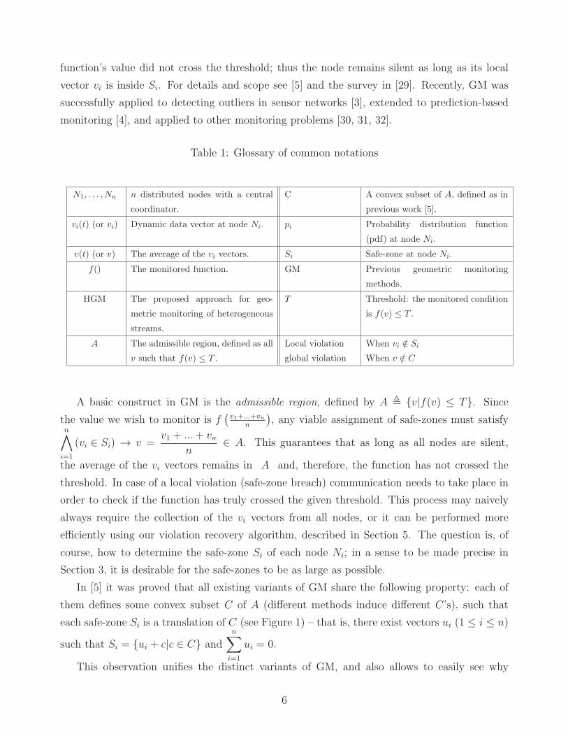
Table 1: Glossary of common notations
N1, . . . , Nn n distributed nodes with a central
coordinator.
C A convex subset of A, defined as in
previous work [5].
vi(t) (or vi) Dynamic data vector at node Ni. pi Probability distribution function
(pdf) at node Ni.
v(t) (or v) The average of the vi vectors. Si Safe-zone at node Ni.
f() The monitored function. GM Previous geometric monitoring
methods.
HGM The proposed approach for geo-
metric monitoring of heterogeneous
streams.
T Threshold: the monitored condition
is f(v) ≤ T .
A The admissible region, defined as all
v such that f(v) ≤ T .
Local violation
global violation
When vi /∈ Si
When v /∈ C
A basic construct in GM is the admissible region, defined by A , {v|f(v) ≤ T}. Since
the value we wish to monitor is f(
v1+...+vnn
)
, any viable assignment of safe-zones must satisfyn∧
i=1
(vi ∈ Si) → v =v1 + ...+ vn
n∈ A. This guarantees that as long as all nodes are silent,
the average of the vi vectors remains in A and, therefore, the function has not crossed the
threshold. In case of a local violation (safe-zone breach) communication needs to take place in
order to check if the function has truly crossed the given threshold. This process may naively
always require the collection of the vi vectors from all nodes, or it can be performed more
efficiently using our violation recovery algorithm, described in Section 5. The question is, of
course, how to determine the safe-zone Si of each node Ni; in a sense to be made precise in
Section 3, it is desirable for the safe-zones to be as large as possible.
In [5] it was proved that all existing variants of GM share the following property: each of
them defines some convex subset C of A (different methods induce different C’s), such that
each safe-zone Si is a translation of C (see Figure 1) – that is, there exist vectors ui (1 ≤ i ≤ n)
such that Si = {ui + c|c ∈ C} andn
∑
i=1
ui = 0.
This observation unifies the distinct variants of GM, and also allows to easily see why
6

AC
1N nN
1S nS
violation
Figure 1: Schematic description of the GM method. A convex subset C of the admissible region
A is determined, and then each node Nk is assigned a safe-zone which is a translation of C.
n∧
i=1
(vi ∈ Si) implies that v = v1+...+vnn
∈ C ⊆ A – it follows immediately from the fact that
convex subsets are closed under taking averages and from the fact that the ui vectors sum to
zero. Methods for constructing C include:
• The method of bounding spheres [2]. A point p ∈ A (the “reference point”) is defined to
be the average of the vectors vi(0), and C is defined as the set of all points q such that
the ball whose diameter is the segment pq is entirely contained in A (see Fig. 2).
Figure 2: “Bounding spheres” approach. The point q1 belongs to C, since the ball whose
diameter is the segment pq1 is contained in A; however, q2 does not belong to C, as the
corresponding ball is not contained in A.
• “Shape sensitive geometric monitoring” [28, 5]. In this approach the bounding spheres
algorithm was improved by a better choice of the reference point p, as well as replacing
the bounding spheres by ellipsoids whose parameters approximate the distribution of the
data at the nodes (but with the underlying assumption that this distribution is shared
by all nodes).
• The “optimized safe-zones” approach, briefly introduced in [5], consists of searching for a
subset C of A which is both convex and “good”, in the sense that∫
C
p(v)dv is large, where
p(v) is the probability density function (termed as pdf hereafter) of the data distribution.
7

The motivation is straightforward – as the integral becomes larger, then on the average
it will take the data vectors more time to exit C.
In this paper we assume that C is given; it can be provided by any of the abovementioned
methods (obviously, if A itself is convex, we just choose C = A). We propose to extend previous
work in a more general direction. Our goal here is to handle a basic problem which haunts all
the existing GM variants: the shapes of the safe-zones at different nodes are identical. Thus,
if the data is heterogeneous across the distinct streams (an example is depicted in Figure 3),
meaning that the data at different nodes obeys different distributions, existing GM algorithms
will perform poorly, causing many local violations that do not correspond to global threshold
crossing (false alarms).
C
1N 2N
1S
2S
Figure 3: Why GM may fail for heterogeneous streams. Here C is equal to a square, and
the data distribution at the two nodes is schematically represented by samples. In GM, the
safe-zones at both nodes are restricted to be a translation of C, and thus cannot cover the data;
HGM will allow much better safe-zones (see Section 3, and Figure 4).
In this paper, we present a more general approach that allows to assign differently shaped
safe-zones to different nodes. As we will shortly demonstrate, our approach requires tackling a
difficult optimization problem, for which practical solutions need to be devised.
3 Safe-Zone Design as an Optimization Problem
We now seek to formulate an optimization problem, whose output is the safe-zones at all nodes.
The safe-zones should satisfy the following properties:
Correctness: If Si denotes the safe-zone at node Ni, we must have:n∧
i=1
(vi ∈ Si) →v1 + ...+ vn
n∈ C. This ensures that every threshold crossing by f(v) will result
in a safe-zone breach in at least one node, that is, all global violations are captured.
8

Expansiveness: Every safe-zone breach (local violation) triggers communication, so the safe-
zones should be as “large” as possible. We measure the “size” of a safe-zone Si by its probability
volume, defined as∫
Si
pi(v)dv where pi is the pdf of the data at node Ni. Probabilistic models
have proved useful in predicting missing and future stream values in various monitoring and
processing tasks [19, 20, 33], including previous geometric methods [5], and their incorporation
in our algorithms proved useful in monitoring real data (Section 6).
Simplicity: At each time step, every node must check whether its data vector is in its safe-
zone. To render this task computationally feasible (especially for thin nodes, such as sensors) it
is desirable that the safe-zones be simple geometric constructs. The simplicity of the safe-zones
is governed by the user, as he/she defines the family of shapes to which the safe-zones belong
(Sections 4.2, 6.1.2).
To handle the correctness and expansiveness requirements, we formulate a constrained op-
timization problem as follows:
Given: (1) probability distribution functions p1, . . . , pn at n nodes
(2) A convex subset C of the admissible region A
Maximize∫
S1
p1dv1 · ... ·∫
Sn
pndvn (expansiveness)
Subject to S1⊕···⊕Sn
n⊆ C (correctness)
where S1⊕···⊕Sn
n=
{
v1+···+vnn
|v1 ∈ S1, . . . , vn ∈ Sn
}
, or the Minkowski sum [34] of S1, . . . , Sn,
in which every element is divided by n (the Minkowski average). Introducing the Minkowski
average is necessary in order to guarantee correctness, since vi must be able to range over the
entire safe-zone Si. Note that instead of using the constraint S1⊕...⊕Sn
n⊆ A, we use S1⊕...⊕Sn
n⊆ C.
This preserves correctness, since C ⊆ A. The reason we chose to use C is that, as it turns out,
typically it’s much easier to check the constraint for the Minkowski average containment in a
convex set; this is discussed in Section 4.4.
To derive the target function∫
S1
p1dv1 · ... ·∫
Sn
pndvn, which estimates the probability that
the local vectors of all nodes will remain in their safe-zones, we assumed that the data is not
correlated between nodes, as it was the case in the experiments in Section 6 (see also [20]
and the discussion therein). If the data is correlated, the algorithm is essentially the same,
with the expression for the probability that data at some node breaches its safe-zone modified
accordingly. We plan to target such cases in the future.
Note that correctness and expansiveness have to reach a “compromise”: figuratively speak-
ing, the correctness constraint restricts the size of the safe-zones, while the probability volume
9

increases as the safe-zones become larger. This trade-off is central in the solution of the opti-
mization problem.
The advantage of the resulting safe-zones is demonstrated by a schematic example (Figure 4),
in which C and the stream pdfs are identical to those in Figure 3. In HGM, however, the
individual safe-zones can be shaped very differently from C, allowing a much better coverage
of the pdfs, while adhering to the correctness constraint. Intuitively speaking, nodes can trade
“geometric slack” between them; here S1 trades “vertical slack” for “horizontal slack”.
1N2N
1S
2S
2
1S 2S
C
Figure 4: Schematic example of HGM safe-zone assignment for two nodes, which also demon-
strates the advantage over previous work. The convex set C is a square, and the pdf at the
left (right) node is uniform over a rectangle elongated along the horizontal (vertical) direction.
HGM can handle this case by assigning the two rectangles S1, S2 as safe-zones, which satisfies
the correctness requirement (since their Minkowski average is equal to C). GM (Figure 3) will
perform poorly in this case.
The Complexity of the Safe-Zone Problem. The input to the safe-zone problem consists
of C and the probability distributions pi. The difficulty of the problem increases with the
number of nodes, the dimensionality of the data, and the complexity of the pis. In Section 7
we prove that the problem is NP-hard and inapproximable. In the next section, we thus seek
to devise practical algorithms to solve this problem.
4 Constructing the Safe-Zones
We now briefly describe the overall operation of the distributed nodes. The computation of
the safe-zones is initially performed by a coordinator node, using a process described in this
section. This process is performed infrequently, since there is no need to modify the safe-zone
10
of a node unless a global threshold violation occurs. As described in Section 3, the input to the
algorithm is: (1) The probability distribution functions p1, . . . , pn at the n nodes. These pdfs
can be of any kind (e.g., Gaussian [28], random walk [25], uniform, etc). Moreover, these pdfs
may be given either analytically or by a sample. As discussed in Section 4.5, message passing
between the nodes and the coordinator in this initial phase can be reduced by using compact
data representations; (2) A convex subset C of the admissible region A.
After the individual safe-zones have been computed, they are assigned to each node. This
process is the end of the initialization stage. Each node Nk does not initiate communication as
long as vk(t) ∈ Sk. If vk(t) /∈ Sk (local violation) the algorithm described in Section 5 is applied
to try and resolve the violation.
4.1 Solving the Optimization Problem
In order to efficiently solve our optimization problem, we need to answer several questions:
• What kinds of shapes to consider for candidate safe-zones? This is discussed in Section 4.2.
• The target function is defined as the product of integrals of the respective pdfs on the
candidate safe-zones. Given candidate safe-zones, how do we efficiently compute the target
function? This is discussed in Section 4.3.
• Given candidate safe-zones, how do we efficiently test if their Minkowski average lies in C?
This is discussed in Section 4.4.
• As we will point out, the number of variables to optimize over is very large, with this number
increasing with the number of nodes. It is well-known that the computational cost of general
optimization routines increases at a super-linear rate with the number of variables. To remedy
this issue, we propose in Section 4.5 a hierarchical clustering approach, which uses a divide-
and-conquer algorithm to reduce the problem to that of recursively computing safe-zones for
small numbers of nodes.
4.2 Shape of Safe-Zones to Consider
The first step in solving an optimization problem is determining the parameters to optimize over.
Here, the space of parameters is huge – all subsets of the Euclidean space are candidates for
safe-zones. The space of all subsets is extremely complicated: not only is it infinite-dimensional,
but also non-linear [35]. For one-dimensional (scalar) data, intervals provide a reasonable choice
for safe-zones, but for higher dimensions no clear candidate exists.
To achieve a practical solution, we choose the safe-zones from a parametric family of shapes,
denoted by S. This family of shapes should satisfy the following requirements:
11
• It should be broad enough so that its members can reasonably approximate every subset
which is a viable candidate for a safe-zone. If this does not hold, the solution may be grossly
sub-optimal. This point is discussed and explained in Section 6.1.2.
• The members of S should have a relatively simple shape (the “simplicity” property, Section
3). In practice, this means that they are polytopes with a restricted number of vertices, or
can be defined by a small number of implicit equations (e.g., polynomials [36]). See further
discussion in Section 6.1.2.
• It should not be too difficult to compute the integral of the various pdfs over members of S
(Section 4.3).
• It should not be too difficult to compute, or bound, the Minkowski average of members of S
(Section 4.4).
The last two conditions allow efficient optimization. If computing the integrals of the pdf or
the Minkowski average are time consuming, the optimization process may be lengthy. We thus
considered and applied in our algorithms various polytopes (such as triangles, boxes, or more
general polytopes) as safe-zones, a choice which yielded good results for the simpler problem in
[5].
As explained in the experimental evaluation (see discussion in Section 6.1.2), this choice
depends on the function f(). However, the challenge of choosing the best shape for arbitrary
functions and data distributions is, by itself, quite formidable; we now elaborate on a very
general paradigm to obtain a good choice.
Bayesian model selection. We propose to view the problem of choosing the family of
safe-zones to optimize over as an instance of the model selection problem. Very often, it is
required to fit a model (e.g. a polynomial approximation) to data. This model is chosen from
a graded family of models of increasing complexity and descriptive power: for polynomials the
models are ordered by their degree, in our case the safe-zones are ordered by the number of
their vertices. One must choose the sub-family of the model to be used (e.g. the degree of the
polynomial or the number of safe-zone vertices). The optimal choice achieves a tradeoff between
the approximation quality of the model and the number of its parameters (in that regard, it
resembles the minimum length description paradigm [37]); obviously, the approximation quality
increases with the number of parameters, but eventually it is “saturated”, meaning that adding
more parameters hardly affects the quality, leads to overfitting, and violates the “simplicity of
the safe-zone” demand (Section 3). To obtain the optimal choice, we have applied Bayesian
model selection [38, 39]. Space does not permit to survey the derivations, so we will just provide
the result:
Lemma 1 For any natural number m, denote by Fm the solution of the safe-zone assignment
12

problem which applies polytopes with m vertices, and denote the value of the target function by
Em. The optimal model is the one which maximizes log(Em)+c |Hm|1
2 , where Hm is the Hessian
matrix of the solution parameters, and c a constant which depends only on the dimension of the
data vectors. The expression log(Em) + c |Hm|1
2 is referred to as the model evidence.
The practical meaning of this criterion is the following: as m increases, we obtain a better
approximation of the pdf’s at the nodes, hence log(Em) increases. However, since the safe-
zones will eventually “saturate” the pdf’s (meaning that increasing m only slightly increases the
target function), the optimal fit becomes very “flat” in parameter space, hence the determinant
of the Hessian will become very small. Bayesian model selection thus provides a rigorous choice
of a model which obtains the optimal tradeoff between the quality of the model and the number
of parameters. To quickly find the optimal m, binary search can be applied.
In the experiments (Section 6) we applied both Bayesian model selection and simple safe-
zones (triangles and boxes), for monitoring non-linear, non-monotonic functions.
A note on the complexity of the problem. The optimization problem we must solve to
obtain the safe-zones is quite more demanding than that in [5], which uses the same safe-zone
for each node. For example, suppose that the data vectors are two-dimensional, there are 100
nodes, and we apply octagonal safe-zones. The optimization problem in [5] requires optimizing
over 16 parameters (8 vertices for the single octagonal safe-zone common to all nodes, with each
vertex having two coordinates), but for the general case treated here, an octagonal region should
be defined for every node, yielding a total of 1,600 parameters. Further, the Minkowski sum
constraint, S1⊕...⊕Sn
n⊆ C, introduces a coupling between the parameters, making it impossible to
separate the optimization problem into disjoint problems with a smaller number of parameters.
No simple solution to this problem exists, since it is NP-hard and inapproximable (Section 7).
4.3 Computing the Target Function
The target function is defined as the product of integrals of the respective pdfs on the candidate
safe-zones. Typically, data is provided as discrete samples. The integral can be computed by
first approximating the discrete samples by a continuous pdf, and then integrating it over the
safe-zone. We used this approach, fitting a GMM (Gaussian Mixture Model) to the discrete
data and integrating it over the safe-zones, which were defined as polytopes. To accelerate the
computation of the integral, we used Green’s Theorem to reduce a double integral to a one-
dimensional integral over the polygon’s boundary: the integral of a general two-dimensional
Gaussian in x, y, exp (− (A2 +Bxy + C2 +Dx+ Ey + F )) over a region R equals the integral
of√π
2√Aexp
(
−(
Ey + Cy2 + F − (D+By)2
4A
))
erf(√
Ax+ D+By
2√A
)
over R’s boundary. For higher
13
dimensions, the integral can also be reduced to integrals of lower dimensions, or computed
using Monte-Carlo methods.
4.4 Checking the Constraints
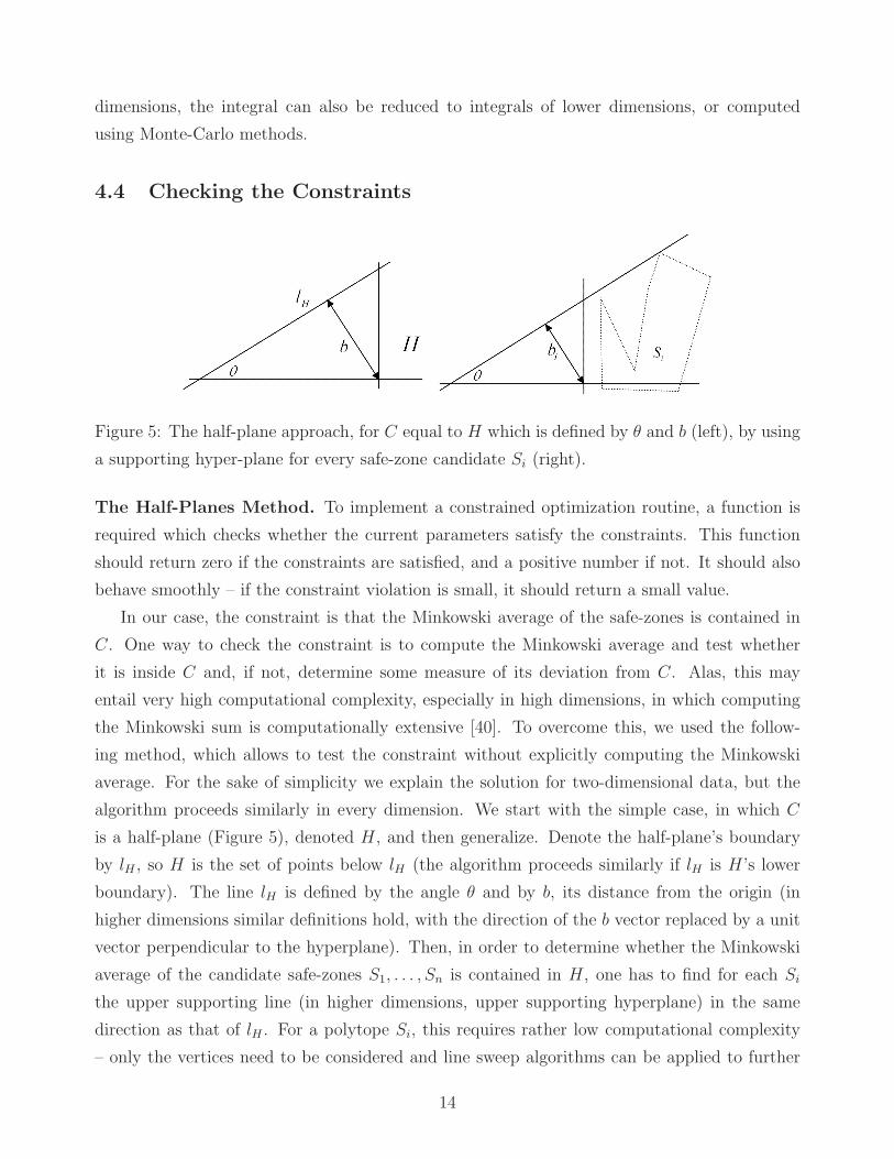
Figure 5: The half-plane approach, for C equal to H which is defined by θ and b (left), by using
a supporting hyper-plane for every safe-zone candidate Si (right).
The Half-Planes Method. To implement a constrained optimization routine, a function is
required which checks whether the current parameters satisfy the constraints. This function
should return zero if the constraints are satisfied, and a positive number if not. It should also
behave smoothly – if the constraint violation is small, it should return a small value.
In our case, the constraint is that the Minkowski average of the safe-zones is contained in
C. One way to check the constraint is to compute the Minkowski average and test whether
it is inside C and, if not, determine some measure of its deviation from C. Alas, this may
entail very high computational complexity, especially in high dimensions, in which computing
the Minkowski sum is computationally extensive [40]. To overcome this, we used the follow-
ing method, which allows to test the constraint without explicitly computing the Minkowski
average. For the sake of simplicity we explain the solution for two-dimensional data, but the
algorithm proceeds similarly in every dimension. We start with the simple case, in which C
is a half-plane (Figure 5), denoted H, and then generalize. Denote the half-plane’s boundary
by lH , so H is the set of points below lH (the algorithm proceeds similarly if lH is H’s lower
boundary). The line lH is defined by the angle θ and by b, its distance from the origin (in
higher dimensions similar definitions hold, with the direction of the b vector replaced by a unit
vector perpendicular to the hyperplane). Then, in order to determine whether the Minkowski
average of the candidate safe-zones S1, . . . , Sn is contained in H, one has to find for each Si
the upper supporting line (in higher dimensions, upper supporting hyperplane) in the same
direction as that of lH . For a polytope Si, this requires rather low computational complexity
– only the vertices need to be considered and line sweep algorithms can be applied to further
14
reduce running time. In order for the Minkowski average of the Si’s to be contained in H,
it is sufficient that∑
bin
≤ b. This algorithm also allows to measure the amount of constraint
violation, which depends on the value of∑
bin
− b.
If C is a convex polytope, then C is equal to the intersection of half-planes, and the measure
of constraint violation is defined as the max (using the sum is also plausible) of the measures
corresponding to the individual half-planes. A general convex C can be efficiently approximated
by an inscribed convex polytope [41]. Alternatively, the following method can be used.
The Direct Method. A more direct method to test the Minkowski sum constraint relies on
the following result [42]:
Lemma 2 If P and Q are convex polytopes with vertices {Pi}, {Qj}, then P ⊕ Q is equal to
the convex hull of the set {Pi +Qj}.
Now, assume we wish to test whether the Minkowski average of P and Q is contained in C.
Since C is convex, it contains the convex hull of every of its subsets; hence it suffices to test
whether the points (Pi + Qj)/2 are in C, for all i, j. If not all points are inside C, then the
constraint violation can be measured by the maximal distance of a point (Pi +Qj)/2 from C’s
boundary. The method easily generalizes to more polytopes: for three polytopes it is required
to test the average of all triplets of vertices, etc.
Comparison of the Half-Planes and Direct Methods. Assume candidate safe-zones
S1, . . . , Sn, where Si has V (Si) vertices. Since in the half-planes method the position of every
half-plane vs. every summand is computed separately, the running time is proportional to
HC
∑n
i=1 V (Si), where HC is the number of half-planes defining C. The running time of the
direct method is proportional to tC∏n
i=1 V (Si), where tC is the time required for checking if a
point is inside C. Given the types of the candidate safe-zones, their number, and the definition
of C, one can choose the method with the lower computational complexity. For example, when
many nodes are present, the half-planes method will usually do better. If C is defined by an
implicit equation g() (e.g., an ellipsoid) then testing for the presence of a point v in C is easy
(i.e., v ∈ C iff g(v) ≤ 0), and the direct method is then better (unless∏n
i=1 V (Si) is large enough
to offset this advantage). In Section 6 some examples are given as to how these considerations
are applied.
4.5 Hierarchical Clustering
While the algorithms presented in Sections 4.3-4.4 reduce the running time for computing
the safe-zones, our optimization problem still poses a formidable difficulty. For example, as
15
discussed in Section 4.2, fitting octagonal safe-zones to 100 nodes with two-dimensional data
requires to optimize over 1,600 variables, which is quite high for a general optimization problem.
To alleviate this problem, we first organize the nodes in a hierarchical structure, which allows
us to then solve the problem recursively (top-down in this hierarchical structure) by reducing
it to sub-problems, each containing a much smaller number of nodes.
We first perform a bottom-up hierarchical clustering of the nodes. To achieve this, a distance
measure between nodes needs to be defined. Since a node is represented by its data vectors,
a distance measure should be defined between subsets of the Euclidean space. We apply the
method in [43], which defines the distance between sets by the L2 distance between their moment
vectors (vectors whose coordinates are low-order moments of the set). The moments have to
be computed only once, in the initialization stage. The leaves of the cluster tree are individual
nodes, and the inner vertices can be thought of as “super nodes”, each containing the union
(Minkowski average) of the data of nodes in the respective sub-tree. Since the moments of
a union of sets are simply the sum of the individual sets’ moments, the computation of the
moment vectors for the inner nodes is very fast.
After the hierarchical clustering is completed, the safe-zones are assigned top-down: first, the
children of the root are assigned safe-zones under the constraint that their Minkowski average is
contained in C 1. In the next level, the grandchildren of the root are assigned safe-zones under
the constraint that their Minkowski average is contained in their parent nodes’ safe-zones, etc.
The leaves are either individual nodes, or clusters which are uniform enough and can all be
assigned safe-zones with identical shapes.
Reducing the Transmitted Parameters. Data should be sent from the nodes to the
coordinator in order to allow computing the safe-zones, and the coordinator has to send the
nodes the definition of their safe-zones. In our experiments this was achieved not by passing
the entire data, but the far more compact parameters of the pdf and the first and second order
moments of the data, which suffice to compute the safe-zones. If the data at the nodes is
very large, we may use a sample to compute its moments. Sending the safe-zone parameters
to the nodes is also very fast, as the safe-zones are described by a relatively small number of
parameters.
5 Violation Recovery
Recall that we define a local violation at time t at Ni if its local vector vi(t) wandered out of
its safe-zone Si. A global violation occurs when the average of the vectors in all nodes exits C.
1This proceeds using the same algorithms described in Sections 4.3-4.4
16
Clearly, a global violation implies at least one local violation, however the opposite may not
be true, in which case the local violation constitutes a false alarm, which should be detected
as such and resolved with minimal communication. Often, a different node can remedy the
violation: assume that the current local vector vj(t) at Nj satisfies vi(t)+vj(t) ∈ Si⊕Sj. Then,
Ni and Nj “balance” each other and the local violation is resolved with minimal communication
overhead (the only communication is between nodes Ni and Nj, either directly or through the
coordinator). In previous work [2, 28] the coordinator randomly chose nodes in an attempt
to balance local violations. Here, we present a more rigorous and efficient method, based on
partitioning the collection of nodes to disjoint pairs which optimally balance each other. This
proceeds as follows: denoting the data set of node Ni by Di, define a non-directed, weighted,
complete graph over the nodes with the weight of the edge connecting Ni and Nj given by
w(i, j) = Pr(xi + xj ∈ Si ⊕ Sj)|xi ∈ Di ∧ xj ∈ Dj). These weights are all computed at
the coordinator. Please note that w(i, j) can also be computed from the pdfs of the nodes,
transmitted to the coordinator in a compact manner, as described at the end of Section 4.5.
Then, perform a maximal perfect matching in this graph. The weight of an edge between two
nodes is defined as the percentage of pairs of data vectors from both nodes whose sum is in
the Minkowski sum of the nodes’ safe-zones; therefore, the larger the weight, the higher the
probability that the two nodes will balance each other. This matching partitions the nodes into
disjoint pairs which have an overall high probability to resolve each other’s local violations.
Please note that if every node Ni simply attempts to balance with node Nj such that w(i, j) is
maximal, the system may quickly run into deadlock when many nodes try to balance with the
same node – this cannot happen with a disjoint partition.
To handle cases in which the optimal pairing fails to resolve the violation, a hierarchical
structure, somewhat resembling the one used for hierarchical clustering, is applied to generalize
the disjoint pairing. Following the optimal pairing of nodes, each pair is viewed as a single node
whose data is the union of the data at both nodes, and maximal perfect matching is performed
on the resulting graph (which has half the number of vertices as the original graph). This
process is continued, with the nodes of the next graph corresponding to quadruples of nodes,
etc. Call the original nodes “Type 1 node”, the pairs obtained in the first maximal perfect
matching “Type 2 nodes”, the nodes corresponding to quadruples “Type 4 nodes” etc. When
the safe-zone at a Type 1 node (i.e., node Ni) is breached, the coordinator attempts to resolve
the violation with Ni’s partner in the Type 2 node it belongs to. If unsuccessful, it attempts to
resolve the violation with the nodes that belong in the subtree of its partner in the Type 4 node
it belongs to: if the Type 4 node containing Ni also contains nodes Nj, Nk, Nl, the violation is
resolved if vi(t) + vj(t) + vk(t) + vl(t) ∈ Si ⊕ Sj ⊕ Sk ⊕ Sl, etc. The overall operation requires
17
log(n) rounds in the worst case, which helps bound its latency.
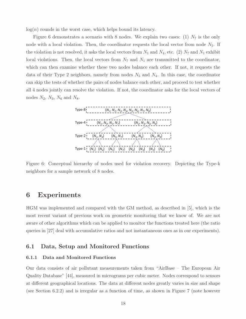
Figure 6 demonstrates a scenario with 8 nodes. We explain two cases: (1) N7 is the only
node with a local violation. Then, the coordinator requests the local vector from node N5. If
the violation is not resolved, it asks the local vectors from N1 and N4, etc. (2) N7 and N1 exhibit
local violations. Then, the local vectors from N7 and N1 are transmitted to the coordinator,
which can then examine whether these two nodes balance each other. If not, it requests the
data of their Type 2 neighbors, namely from nodes N5 and N4. In this case, the coordinator
can skip the tests of whether the pairs of nodes balance each other, and proceed to test whether
all 4 nodes jointly can resolve the violation. If not, the coordinator asks for the local vectors of
nodes N2, N3, N6 and N8.
Type!1
Type!2
Type!4
Type!8 {N1,"N
2,"N
3,"N
4,"N
5,"N
6,"N
7,"N
8}
{N1,"N
4,"N
5,"N
7} {N
2,"N
3,"N
6,"N
8}
{N3,"N
6} {N
2,"N
8}{N
1,"N
4} {N
5,"N
7}
{N1} {N
4} {N
5} {N
7} {N
3}{N
6} {N
2} {N
8}
Figure 6: Conceptual hierarchy of nodes used for violation recovery. Depicting the Type-k
neighbors for a sample network of 8 nodes.
6 Experiments
HGM was implemented and compared with the GM method, as described in [5], which is the
most recent variant of previous work on geometric monitoring that we know of. We are not
aware of other algorithms which can be applied to monitor the functions treated here (the ratio
queries in [27] deal with accumulative ratios and not instantaneous ones as in our experiments).
6.1 Data, Setup and Monitored Functions
6.1.1 Data and Monitored Functions
Our data consists of air pollutant measurements taken from “AirBase – The European Air
Quality Database” [44], measured in micrograms per cubic meter. Nodes correspond to sensors
at different geographical locations. The data at different nodes greatly varies in size and shape
(see Section 6.2.2) and is irregular as a function of time, as shown in Figure 7 (note however
18

that we use the pdf of the data values per se, not as a time series). The quality of results was
measured by the amount of reduction in communication, which is proportional to the number
of safe-zone violations.
Figure 7: Typical behavior of NO concentrations at a node as a function of time. The behavior
of NO2 is similar.
The monitored functions were chosen due to their practical importance, and also as they
are non-linear and non-monotonic and, thus, cannot be handled by most existing methods. In
Section 6.2 results are presented for monitoring the ratio of NO to NO2, which is known to be an
important indicator in air quality analysis [45]. In Section 6.3 the chi-square distance between
histograms was monitored for five-dimensional data. An example of monitoring a quadratic
function in three variables is also presented (Section 6.4); quadratic functions are important
in numerous applications (e.g., the variance is a quadratic function in the variables, and a
normal distribution is the exponent of a quadratic function, hence thresholding it is equivalent
to thresholding the quadratic).
6.1.2 Choosing the Family of Safe-Zones
To solve the optimization problem, it is necessary to define a parametric family of shapes
S from which the safe-zones will be chosen. Section 4.2 discusses the properties this family
should satisfy. In [5], the suitability of some families of polytopes is studied for the simpler,
but related, problem of finding a safe-zone common to all nodes. The motivations for choosing
S here were:
• Ratio queries (Section 6.2) – the triangular safe-zones (Figure 8) have the same structure,
but not size or location, as C, and are very simple to define and apply.
• Chi-square monitoring (Section 6.3) – here the motivation was to choose safe-zones with a
very simple shape, which still enabled a very substantial improvement over GM. We thus
applied boxes (hyperrectangles), which are also attractive as they render the computation of
19
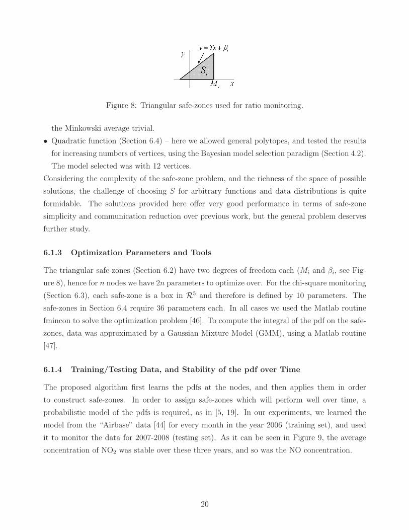
Figure 8: Triangular safe-zones used for ratio monitoring.
the Minkowski average trivial.
• Quadratic function (Section 6.4) – here we allowed general polytopes, and tested the results
for increasing numbers of vertices, using the Bayesian model selection paradigm (Section 4.2).
The model selected was with 12 vertices.
Considering the complexity of the safe-zone problem, and the richness of the space of possible
solutions, the challenge of choosing S for arbitrary functions and data distributions is quite
formidable. The solutions provided here offer very good performance in terms of safe-zone
simplicity and communication reduction over previous work, but the general problem deserves
further study.
6.1.3 Optimization Parameters and Tools
The triangular safe-zones (Section 6.2) have two degrees of freedom each (Mi and βi, see Fig-
ure 8), hence for n nodes we have 2n parameters to optimize over. For the chi-square monitoring
(Section 6.3), each safe-zone is a box in R5 and therefore is defined by 10 parameters. The
safe-zones in Section 6.4 require 36 parameters each. In all cases we used the Matlab routine
fmincon to solve the optimization problem [46]. To compute the integral of the pdf on the safe-
zones, data was approximated by a Gaussian Mixture Model (GMM), using a Matlab routine
[47].
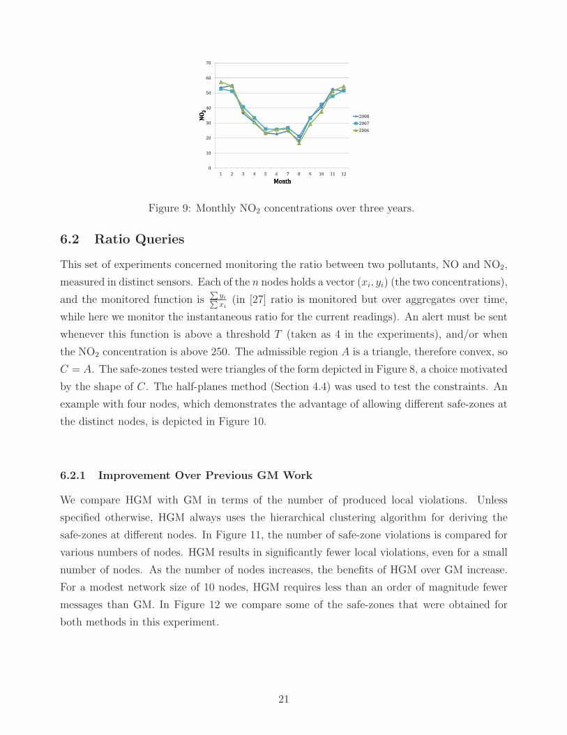
6.1.4 Training/Testing Data, and Stability of the pdf over Time
The proposed algorithm first learns the pdfs at the nodes, and then applies them in order
to construct safe-zones. In order to assign safe-zones which will perform well over time, a
probabilistic model of the pdfs is required, as in [5, 19]. In our experiments, we learned the
model from the “Airbase” data [44] for every month in the year 2006 (training set), and used
it to monitor the data for 2007-2008 (testing set). As it can be seen in Figure 9, the average
concentration of NO2 was stable over these three years, and so was the NO concentration.
20
��
��
��
��
��
��
��
��
��
��
���
���
�
��
�
� � � � � � � �� �� �
���� ���� ���� ����
���
Figure 9: Monthly NO2 concentrations over three years.
6.2 Ratio Queries
This set of experiments concerned monitoring the ratio between two pollutants, NO and NO2,
measured in distinct sensors. Each of the n nodes holds a vector (xi, yi) (the two concentrations),
and the monitored function is∑
yi∑xi
(in [27] ratio is monitored but over aggregates over time,
while here we monitor the instantaneous ratio for the current readings). An alert must be sent
whenever this function is above a threshold T (taken as 4 in the experiments), and/or when
the NO2 concentration is above 250. The admissible region A is a triangle, therefore convex, so
C = A. The safe-zones tested were triangles of the form depicted in Figure 8, a choice motivated
by the shape of C. The half-planes method (Section 4.4) was used to test the constraints. An
example with four nodes, which demonstrates the advantage of allowing different safe-zones at
the distinct nodes, is depicted in Figure 10.
6.2.1 Improvement Over Previous GM Work
We compare HGM with GM in terms of the number of produced local violations. Unless
specified otherwise, HGM always uses the hierarchical clustering algorithm for deriving the
safe-zones at different nodes. In Figure 11, the number of safe-zone violations is compared for
various numbers of nodes. HGM results in significantly fewer local violations, even for a small
number of nodes. As the number of nodes increases, the benefits of HGM over GM increase.
For a modest network size of 10 nodes, HGM requires less than an order of magnitude fewer
messages than GM. In Figure 12 we compare some of the safe-zones that were obtained for
both methods in this experiment.
21
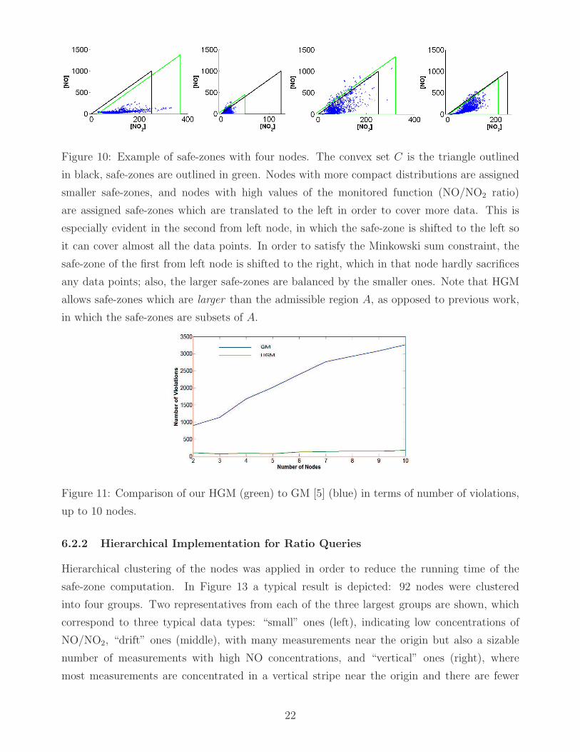
Figure 10: Example of safe-zones with four nodes. The convex set C is the triangle outlined
in black, safe-zones are outlined in green. Nodes with more compact distributions are assigned
smaller safe-zones, and nodes with high values of the monitored function (NO/NO2 ratio)
are assigned safe-zones which are translated to the left in order to cover more data. This is
especially evident in the second from left node, in which the safe-zone is shifted to the left so
it can cover almost all the data points. In order to satisfy the Minkowski sum constraint, the
safe-zone of the first from left node is shifted to the right, which in that node hardly sacrifices
any data points; also, the larger safe-zones are balanced by the smaller ones. Note that HGM
allows safe-zones which are larger than the admissible region A, as opposed to previous work,
in which the safe-zones are subsets of A.
Figure 11: Comparison of our HGM (green) to GM [5] (blue) in terms of number of violations,
up to 10 nodes.
6.2.2 Hierarchical Implementation for Ratio Queries
Hierarchical clustering of the nodes was applied in order to reduce the running time of the
safe-zone computation. In Figure 13 a typical result is depicted: 92 nodes were clustered
into four groups. Two representatives from each of the three largest groups are shown, which
correspond to three typical data types: “small” ones (left), indicating low concentrations of
NO/NO2, “drift” ones (middle), with many measurements near the origin but also a sizable
number of measurements with high NO concentrations, and “vertical” ones (right), where
most measurements are concentrated in a vertical stripe near the origin and there are fewer
22
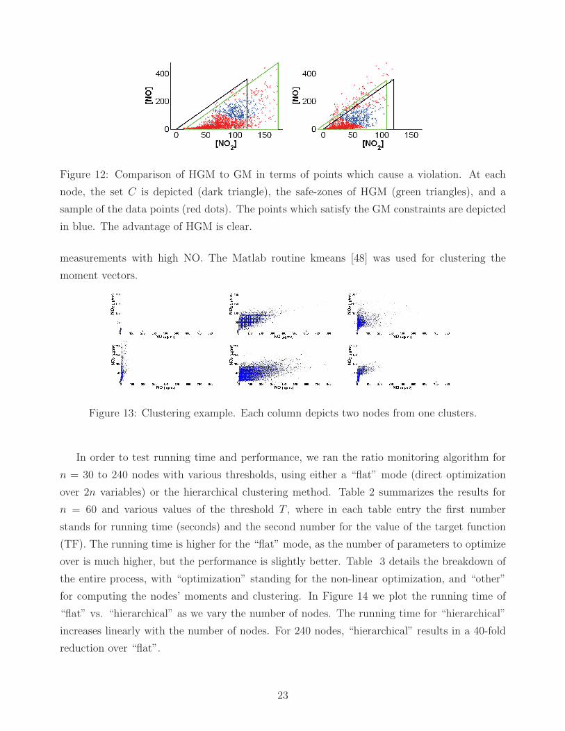
Figure 12: Comparison of HGM to GM in terms of points which cause a violation. At each
node, the set C is depicted (dark triangle), the safe-zones of HGM (green triangles), and a
sample of the data points (red dots). The points which satisfy the GM constraints are depicted
in blue. The advantage of HGM is clear.
measurements with high NO. The Matlab routine kmeans [48] was used for clustering the
moment vectors.
Figure 13: Clustering example. Each column depicts two nodes from one clusters.
In order to test running time and performance, we ran the ratio monitoring algorithm for
n = 30 to 240 nodes with various thresholds, using either a “flat” mode (direct optimization
over 2n variables) or the hierarchical clustering method. Table 2 summarizes the results for
n = 60 and various values of the threshold T , where in each table entry the first number
stands for running time (seconds) and the second number for the value of the target function
(TF). The running time is higher for the “flat” mode, as the number of parameters to optimize
over is much higher, but the performance is slightly better. Table 3 details the breakdown of
the entire process, with “optimization” standing for the non-linear optimization, and “other”
for computing the nodes’ moments and clustering. In Figure 14 we plot the running time of
“flat” vs. “hierarchical” as we vary the number of nodes. The running time for “hierarchical”
increases linearly with the number of nodes. For 240 nodes, “hierarchical” results in a 40-fold
reduction over “flat”.
23
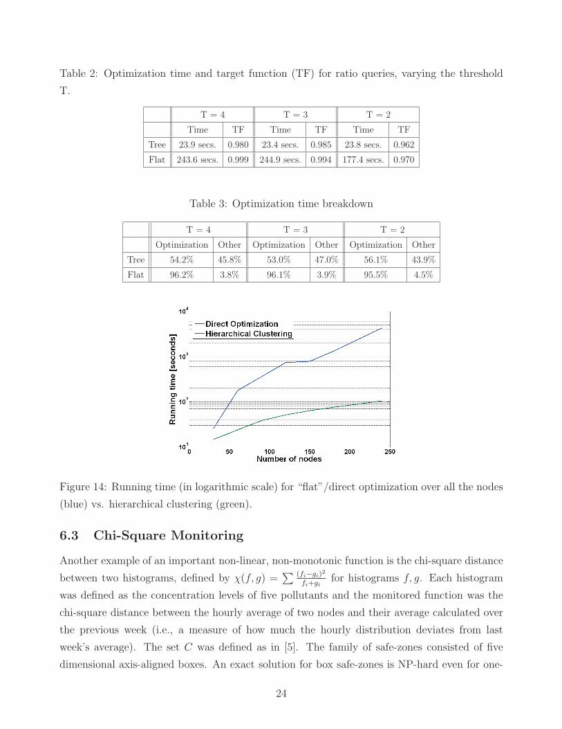
Table 2: Optimization time and target function (TF) for ratio queries, varying the threshold
T.
T = 4 T = 3 T = 2
Time TF Time TF Time TF
Tree 23.9 secs. 0.980 23.4 secs. 0.985 23.8 secs. 0.962
Flat 243.6 secs. 0.999 244.9 secs. 0.994 177.4 secs. 0.970
Table 3: Optimization time breakdown
T = 4 T = 3 T = 2
Optimization Other Optimization Other Optimization Other
Tree 54.2% 45.8% 53.0% 47.0% 56.1% 43.9%
Flat 96.2% 3.8% 96.1% 3.9% 95.5% 4.5%
Figure 14: Running time (in logarithmic scale) for “flat”/direct optimization over all the nodes
(blue) vs. hierarchical clustering (green).
6.3 Chi-Square Monitoring
Another example of an important non-linear, non-monotonic function is the chi-square distance
between two histograms, defined by χ(f, g) =∑ (fi−gi)
2
fi+gifor histograms f, g. Each histogram
was defined as the concentration levels of five pollutants and the monitored function was the
chi-square distance between the hourly average of two nodes and their average calculated over
the previous week (i.e., a measure of how much the hourly distribution deviates from last
week’s average). The set C was defined as in [5]. The family of safe-zones consisted of five
dimensional axis-aligned boxes. An exact solution for box safe-zones is NP-hard even for one-
24
0 100 200 300 400 500
1.2
1
0.8
0.6
0.4
0.2
0
Chi!squ
are"value
Time"(in"hours)
Oscillating!node!
Non"oscillating!node!
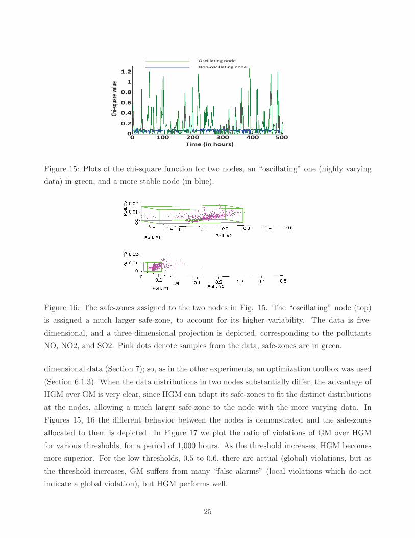
Figure 15: Plots of the chi-square function for two nodes, an “oscillating” one (highly varying
data) in green, and a more stable node (in blue).
Figure 16: The safe-zones assigned to the two nodes in Fig. 15. The “oscillating” node (top)
is assigned a much larger safe-zone, to account for its higher variability. The data is five-
dimensional, and a three-dimensional projection is depicted, corresponding to the pollutants
NO, NO2, and SO2. Pink dots denote samples from the data, safe-zones are in green.
dimensional data (Section 7); so, as in the other experiments, an optimization toolbox was used
(Section 6.1.3). When the data distributions in two nodes substantially differ, the advantage of
HGM over GM is very clear, since HGM can adapt its safe-zones to fit the distinct distributions
at the nodes, allowing a much larger safe-zone to the node with the more varying data. In
Figures 15, 16 the different behavior between the nodes is demonstrated and the safe-zones
allocated to them is depicted. In Figure 17 we plot the ratio of violations of GM over HGM
for various thresholds, for a period of 1,000 hours. As the threshold increases, HGM becomes
more superior. For the low thresholds, 0.5 to 0.6, there are actual (global) violations, but as
the threshold increases, GM suffers from many “false alarms” (local violations which do not
indicate a global violation), but HGM performs well.
25
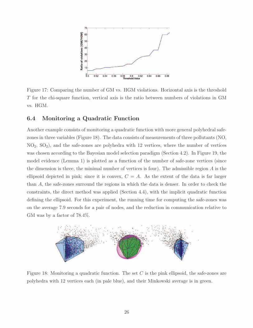
Figure 17: Comparing the number of GM vs. HGM violations. Horizontal axis is the threshold
T for the chi-square function, vertical axis is the ratio between numbers of violations in GM
vs. HGM.
6.4 Monitoring a Quadratic Function
Another example consists of monitoring a quadratic function with more general polyhedral safe-
zones in three variables (Figure 18). The data consists of measurements of three pollutants (NO,
NO2, SO2), and the safe-zones are polyhedra with 12 vertices, where the number of vertices
was chosen according to the Bayesian model selection paradigm (Section 4.2). In Figure 19, the
model evidence (Lemma 1) is plotted as a function of the number of safe-zone vertices (since
the dimension is three, the minimal number of vertices is four). The admissible region A is the
ellipsoid depicted in pink; since it is convex, C = A. As the extent of the data is far larger
than A, the safe-zones surround the regions in which the data is denser. In order to check the
constraints, the direct method was applied (Section 4.4), with the implicit quadratic function
defining the ellipsoid. For this experiment, the running time for computing the safe-zones was
on the average 7.9 seconds for a pair of nodes, and the reduction in communication relative to
GM was by a factor of 78.4%.
Figure 18: Monitoring a quadratic function. The set C is the pink ellipsoid, the safe-zones are
polyhedra with 12 vertices each (in pale blue), and their Minkowski average is in green.
26
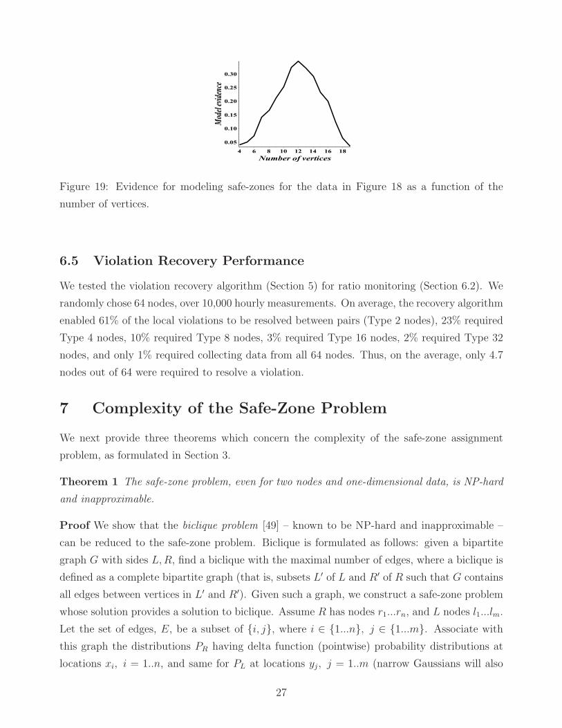
Figure 19: Evidence for modeling safe-zones for the data in Figure 18 as a function of the
number of vertices.
6.5 Violation Recovery Performance
We tested the violation recovery algorithm (Section 5) for ratio monitoring (Section 6.2). We
randomly chose 64 nodes, over 10,000 hourly measurements. On average, the recovery algorithm
enabled 61% of the local violations to be resolved between pairs (Type 2 nodes), 23% required
Type 4 nodes, 10% required Type 8 nodes, 3% required Type 16 nodes, 2% required Type 32
nodes, and only 1% required collecting data from all 64 nodes. Thus, on the average, only 4.7
nodes out of 64 were required to resolve a violation.
7 Complexity of the Safe-Zone Problem
We next provide three theorems which concern the complexity of the safe-zone assignment
problem, as formulated in Section 3.
Theorem 1 The safe-zone problem, even for two nodes and one-dimensional data, is NP-hard
and inapproximable.
Proof We show that the biclique problem [49] – known to be NP-hard and inapproximable –
can be reduced to the safe-zone problem. Biclique is formulated as follows: given a bipartite
graph G with sides L,R, find a biclique with the maximal number of edges, where a biclique is
defined as a complete bipartite graph (that is, subsets L′ of L and R′ of R such that G contains
all edges between vertices in L′ and R′). Given such a graph, we construct a safe-zone problem
whose solution provides a solution to biclique. Assume R has nodes r1...rn, and L nodes l1...lm.
Let the set of edges, E, be a subset of {i, j}, where i ∈ {1...n}, j ∈ {1...m}. Associate with
this graph the distributions PR having delta function (pointwise) probability distributions at
locations xi, i = 1..n, and same for PL at locations yj, j = 1..m (narrow Gaussians will also
27
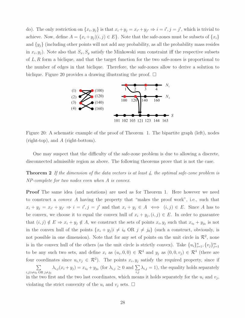
do). The only restriction on {xi, yj} is that xi+yj = xi′ +yj′ ⇒ i = i′, j = j′, which is trivial to
achieve. Now, define A = {xi+ yj|(i, j) ∈ E}. Note that the safe-zones must be subsets of {xi}and {yj} (including other points will not add any probability, as all the probability mass resides
in xi, yj). Note also that Sx, Sy satisfy the Minkowski sum constraint iff the respective subsets
of L,R form a biclique, and that the target function for the two safe-zones is proportional to
the number of edges in that biclique. Therefore, the safe-zones allow to derive a solution to
biclique. Figure 20 provides a drawing illustrating the proof. �
)1(
)2(
)3(
)4(
)100(
)120(
)140(
)160(
1 2 3 4
100 120 140 160
101 102 103 121 123 144 163
1N
2N
S
Figure 20: A schematic example of the proof of Theorem 1. The bipartite graph (left), nodes
(right-top), and A (right-bottom).
One may suspect that the difficulty of the safe-zone problem is due to allowing a discrete,
disconnected admissible region as above. The following theorems prove that is not the case.
Theorem 2 If the dimension of the data vectors is at least 4, the optimal safe-zone problem is
NP-complete for two nodes even when A is convex.
Proof The same idea (and notations) are used as for Theorem 1. Here however we need
to construct a convex A having the property that “makes the proof work”, i.e., such that
xi + yj = xi′ + yj′ ⇒ i = i′, j = j′ and that xi + yj ∈ A ⇐⇒ (i, j) ∈ E. Since A has to
be convex, we choose it to equal the convex hull of xi + yj, (i, j) ∈ E. In order to guarantee
that (i, j) /∈ E ⇒ xi + yj /∈ A, we construct the sets of points xi, yj such that xi0 + yj0 is not
in the convex hull of the points {xi + yj|i 6= i0 OR j 6= j0} (such a construct, obviously, is
not possible in one dimension). Note that for any set of points on the unit circle in R2, none
is in the convex hull of the others (as the unit circle is strictly convex). Take {ui}ni=1, {vj}mj=1
to be any such two sets, and define xi as (ui, 0, 0) ∈ R4 and yj as (0, 0, vj) ∈ R4 (there are
four coordinates since ui,vj ∈ R2). The points xi, yj satisfy the required property, since if∑
i,j|i 6=i0 OR j 6=j0
λi,j(xi + yj) = xi0 + yj0 (for λi,j ≥ 0 and∑
i,j
λi,j = 1), the equality holds separately
in the two first and the two last coordinates, which means it holds separately for the ui and vj,
violating the strict convexity of the ui and vj sets. �
28

Theorem 3 For more than two nodes, the safe-zone problem is NP-Complete when A is a
one-dimensional interval.
Proof We show that the knapsack problem (known to be NP-Complete) can be reduced to the
safe-zone problem. Given a knapsack problem with n objects O1, ..., On, value vi and weight wi
for Oi, and a knapsack which can carry a maximal weight of W , we reduce the problem to a
safe-zone problem. First, we create n nodes N1, ..., Nn, with Ni corresponding to Oi, with the
following pdf:
Pi(x) =
1/C if x = 0
(evi − 1)/C if x = wi
(C − evi)/C if x = W + 1
0 otherwise
(1)
for C = maxi
{evi}. Note that the overall probability at each node equals 1. Now, define A to be
the interval [0,W/n]. Assume we can solve the safe-zone problem with an interval Si = [ai, bi]
for each node Ni. Note that in this solution we may assume that ai = 0 and 0 ≤ bi ≤ W for all
i (it is not possible to take bi > W as this would violate the Minkowski average constraint, and
it will not add anything to take ai < 0, as all the probability mass is in the region x ≥ 0). There
are two types of possible safe-zones at each node: those which contain only the origin, and those
which equal [0, wi]. Denote by S the subset of nodes in which [0, wi] is taken. The solution is
legal iff the Minkowski average of {[0, wi]|i ∈ S} is inside A = [0, Wn], but this is equivalent to
demanding∑
i∈Swi ≤ W – which is exactly the legality condition for the knapsack problem. Also,
the product of the probability volumes at the nodes (which the safe-zone problem attempts to
maximize) clearly equals (∏
i∈Sevi)/Cn, so up to a constant factor it equals e
∑
i∈S
vi. Therefore, the
safe-zone problem is equivalent to maximizing∑
i∈Svi, under the constraint
∑
i∈Swi ≤ W , hence it
determines a solution to the knapsack problem. �
8 Conclusions and Future Work
A method for monitoring threshold queries over heterogeneous distributed streams was pre-
sented. A paradigm for minimizing communication is formulated as an optimization problem
of a geometric and probabilistic flavor, whose solution assigns each node a “safe-zone” with the
property that a node may remain silent as long as its data vector is in its safe-zone. While the
problem is shown to be difficult, a practical solution using a hierarchical clustering algorithm
is presented and implemented for two, three, and five dimensional data, allowing to achieve
29

substantial improvement over previous work, while using rather simple safe-zones which also
reduce the computational effort at the nodes.
We now outline, as space permits, some directions for future work.
• Correlated streams. Here, the data we used was uncorrelated between nodes. If some of
the streams are correlated, the goal will still be to seek an optimized solution as described
in Section 3, the difference being that the overall probability to remain in the distinct
safe-zones will not factor to the product of the probabilities for the individual safe-zones.
• Dynamic change of data distribution within a stream. If the pdfs at some of the
nodes change, the safe-zone optimization process may need to be run again. However, it
may suffice to modify the safe-zones only of the nodes whose pdf changed. To see this,
assume without loss of generality that we have n nodes with safe-zones si, i = 1 . . . n, and
that the pdf at nodes 1 . . . k had changed. We can treat these nodes only, and assign
them new safe-zones S′
i , such that S′
1 ⊕ . . .⊕ S′
k ⊂ S1 ⊕ . . .⊕ Sk. Since Minkowski sums
are monotonic with respect to inclusion, this guarantees that the overall Minkowski sum
(that is, of all n nodes) will still be contained in the set C.
• Handling global violations. If a global violation occurs (that is, f(v) > T ), the
algorithm switches to the monitoring of the condition v ∈ C ′, where C ′ is a convex subset
of A’s complement. A plausible solution is to prepare appropriate safe-zones in advance,
for this case as well as for different values of the threshold T ; the monitoring scheme then
simply switches to the appropriate safe-zones.
References
[1] D. J. Abadi, Y. Ahmad, M. Balazinska, U. Cetintemel, M. Cherniack, J.-H. Hwang, W. Lindner, A. Maskey,A. Rasin, E. Ryvkina, N. Tatbul, Y. Xing, and S. B. Zdonik, “The design of the borealis stream processingengine,” in CIDR, 2005.
[2] I. Sharfman, A. Schuster, and D. Keren, “A geometric approach to monitoring threshold functions overdistributed data streams,” ACM Trans. Database Syst., vol. 32, no. 4, 2007.
[3] S. Burdakis and A. Deligiannakis, “Detecting outliers in sensor networks using the geometric approach,”in ICDE, 2012.
[4] N. Giatrakos, A. Deligiannakis, M. N. Garofalakis, I. Sharfman, and A. Schuster, “Prediction-based geo-metric monitoring over distributed data streams,” in SIGMOD, 2012.
[5] D. Keren, I. Sharfman, A. Schuster, and A. Livne, “Shape sensitive geometric monitoring,” IEEE Trans.Knowl. Data Eng., vol. 24, no. 8, 2012.
[6] G. Sagy, D. Keren, I. Sharfman, and A. Schuster, “Distributed threshold querying of general functions bya difference of monotonic representation,” PVLDB, vol. 4, no. 2, 2010.
[7] G. Cormode and M. N. Garofalakis, “Sketching streams through the net: Distributed approximate querytracking,” in VLDB, 2005.
30
[8] L. Huang, X. Nguyen, M. N. Garofalakis, J. M. Hellerstein, M. I. Jordan, A. D. Joseph, and N. Taft,“Communication-efficient online detection of network-wide anomalies,” in INFOCOM, 2007.
[9] A. Arasu and G. S. Manku, “Approximate counts and quantiles over sliding windows,” in PODS, 2004.
[10] G. Cormode and M. N. Garofalakis, “Histograms and wavelets on probabilistic data,” in ICDE, 2009.
[11] A. Manjhi, V. Shkapenyuk, K. Dhamdhere, and C. Olston, “Finding (recently) frequent items in distributeddata streams,” in ICDE, 2005.
[12] K. Yi and Q. Zhang, “Optimal tracking of distributed heavy hitters and quantiles,” in PODS, 2009.
[13] G. Cormode, M. N. Garofalakis, S. Muthukrishnan, and R. Rastogi, “Holistic aggregates in a networkedworld: Distributed tracking of approximate quantiles,” in SIGMOD, 2005.
[14] G. Cormode, S. Muthukrishnan, and W. Zhuang, “What’s different: Distributed, continuous monitoringof duplicate-resilient aggregates on data streams,” in ICDE, 2006.
[15] G. Cormode, S. Muthukrishnan, K. Yi, and Q. Zhang, “Optimal sampling from distributed streams,” inPODS, 2010.
[16] F. Li, K. Yi, and J. Jestes, “Ranking distributed probabilistic data,” in SIGMOD, 2009.
[17] G. Cormode, S. Muthukrishnan, and K. Yi, “Algorithms for distributed functional monitoring,” in SODA,2008.
[18] C. Arackaparambil, J. Brody, and A. Chakrabarti, “Functional monitoring without monotonicity,” inICALP (1), 2009.
[19] A. Deshpande, C. Guestrin, S. Madden, J. M. Hellerstein, and W. Hong, “Model-driven data acquisitionin sensor networks,” in VLDB, 2004.
[20] M. Tang, F. Li, J. M. Phillips, and J. Jestes, “Efficient threshold monitoring for distributed probabilisticdata,” in ICDE, 2012.
[21] R. Keralapura, G. Cormode, and J. Ramamirtham, “Communication-efficient distributed monitoring ofthresholded counts,” in SIGMOD, 2006.
[22] K. Yoshihara, K. Sugiyama, H. Horiuchi, and S. Obana, “Dynamic polling scheme based on time variationof network management information values,” in Proceedings of 11th IFIP/IEEE International Symposiumon Integrated Network Management, 1999.
[23] D. P. Woodruff and Q. Zhang, “Tight bounds for distributed functional monitoring,” in STOC, 2012, pp.941–960.
[24] R. Wolff, K. Bhaduri, and H. Kargupta, “A generic local algorithm for mining data streams in largedistributed systems,” IEEE Trans. on Knowl. and Data Eng., vol. 21, no. 4, 2009.
[25] S. Shah and K. Ramamritham, “Handling non-linear polynomial queries over dynamic data,” in ICDE,2008.
[26] S. Michel, P. Triantafillou, and G. Weikum, “Klee: a framework for distributed top-k query algorithms,”in VLDB ’05. VLDB Endowment, 2005.
[27] R. Gupta, K. Ramamritham, and M. K. Mohania, “Ratio threshold queries over distributed data sources,”in ICDE, 2010.
[28] I. Sharfman, A. Schuster, and D. Keren, “Shape sensitive geometric monitoring,” in PODS, 2008.
[29] G. Cormode, “Algorithms for continuous distributing monitoring: A survey,” in AlMoDEP, 2011.
[30] J. Kogan, “Feature selection over distributed data streams through optimization,” in SDM, 2012.
[31] O. Papapetrou, M. N. Garofalakis, and A. Deligiannakis, “Sketch-based querying of distributed sliding-window data streams,” PVLDB, vol. 5, no. 10, 2012.
[32] M. N. Garofalakis, D. Keren, and V. Samoladas, “Sketch-based geometric monitoring of distributed streamqueries,” PVLDB, 2013.
31
[33] B. Kanagal and A. Deshpande, “Online filtering, smoothing and probabilistic modeling of streaming data,”in ICDE, 2008.
[34] J. Serra, “Image analysis and mathematical morphology,” in Academic Press, London, 1982.
[35] B. Wirth, L. Bar, M. Rumpf, and G. Sapiro, “A continuum mechanical approach to geodesics in shapespace,” International Journal of Computer Vision, vol. 93, no. 3, 2011.
[36] D. Keren, D. B. Cooper, and J. Subrahmonia, “Describing complicated objects by implicit polynomials,”IEEE Trans. Pattern Anal. Mach. Intell., vol. 16, no. 1, 1994.
[37] J. Rissanen, “A universal prior for integers and estimation by minimum description length,” The Annalsof statistics, vol. 11, no. 2, pp. 416–431, 1983.
[38] D. Mackay, “Bayesian interpolation,” Neural Computation, vol. 4, pp. 415–447, 1992.
[39] J. Subrahmonia, D. B. Cooper, and D. Keren, “Practical reliable bayesian recognition of 2d and 3d objectsusing implicit polynomials and algebraic invariants,” IEEE Trans. Pattern Anal. Mach. Intell., vol. 18,no. 5, pp. 505–519, 1996.
[40] H. R. Tiwary, “On the hardness of minkowski addition and related operations,” in Symposium on Compu-tational Geometry, 2007.
[41] Y. Gordon, M. Meyer, and S. Reisner, “Constructing a polytope to approximate a convex body,” inGeometriae Dedicata, 1995.
[42] E. Fogel and D. Halperin, “Exact and efficient construction of minkowski sums of convex polyhedra withapplications,” Computer-Aided Design, vol. 39, no. 11, 2007.
[43] M. Elad, A. Tal, and S. Ar, “Content based retrieval of vrml objects: an iterative and interactive approach,”in Multimedia 2001, 2002.
[44] “The european air quality database,” in http://tinyurl.com/ct9bh7x.
[45] M. Kurpius and A. Goldstein, “Gas-phase chemistry dominates o3 loss to a forest, implying a source ofaerosols and hydroxyl radicals to the atmosphere,” Geophysical Research Letters, vol. 30, no. 7, 2007.
[46] http://tinyurl.com/kxssfgl.
[47] DCPR (Data Clustering and Pattern Recognition) Toolbox, http://tinyurl.com/nxospq2.
[48] http://www.mathworks.com/help/toolbox/stats/kmeans.html.
[49] C. Ambuhl, M. Mastrolilli, and O. Svensson, “Inapproximability results for maximum edge biclique, mini-mum linear arrangement, and sparsest cut,” SIAM J. Comput., vol. 40, no. 2, 2011.
Author biographies:
Daniel Keren (Ph.D. 1991, Hebrew University in Jerusalem) is with the computer science
department in Haifa University, Haifa, Israel. Prof. Keren’s main fields of research are geom-
etry and probability. He published mostly in computer vision journals and conferences. Since
2003, he has been working closely with Prof. Assaf Schuster’s group at the Technion, in the
area of distributed monitoring. His main contribution is in the mathematical aspects of the
research such as object modelling, learning, optimization, and probability. A main novelty of
the joint research is the incorporation of such mathematical tools into the research paradigm;
this allowed to develop new methodologies, based on geometry, to monitor general functions.
32

Guy Sagy completed his Ph.D. at the Computer Science Faculty, the Technion, in 2011. His
main areas of research are distributed algorithms and geometric methods for stream processing.
Izchak Sharfman completed his Ph.D. at the Computer Science Faculty, the Technion, in
2008. His main areas of research are distributed algorithms and geometric methods for stream
processing. He is currently a post-doctoral researcher in the Technion.
Amir Abboud graduated with a B.Sc. from the “Etgar” program at Haifa University,
completed his M.Sc. at the Technion, and is currently a Ph.D. student at Stanford University.
David Ben-David graduated with an M.Sc from the Computer Science Faculty in the
Technion, 2012. His work concerned distributed monitoring. He is currently a software engineer
at EMC, Israel.
Assaf Schuster has established and is managing DSL, the Distributed Systems Laboratory
(http://dsl.cs.technion.ac.il). Several CS faculty members see DSL as the main scope hosting
their applied and systems research, with about 35 graduate and hundreds of undergraduate
students working in the lab during the academic year. DSL is supported by Intel, Microsoft,
Sun, IBM, and other interested partners. Prof. Schuster is well known in the area of parallel,
distributed, high performance, and grid computing. He published over 160 papers in those areas
in high-quality conferences and journals. He regularly participates in program committees for
conferences on parallel and distributed computing. He consults the hi-tech industry on related
issues and holds seven patents. He serves as an associate editor of the Journal of Parallel and
Distributed Computing, and IEEE Transactions on Computers. He supervises seven Ph.D.
students and ten M.Sc. students, and takes part in large national and EU projects as an expert
on grid and distributed computing.
Antonios Deligiannakis is an Assistant Professor of Computer Science at the Dept. of
Electronic & Computer Engineering of the Technical Univ. of Crete, as of January 2008.
He received the Diploma degree in Electrical and Computer Engineering from the National
Technical Univ. of Athens in 1999, and the MSc and PhD degrees in Computer Science from the
Univ. of Maryland in 2001 and 2005, respectively. He then performed his PostDoctoral research
at the Dept. of Informatics and Telecommunications of the Univ. of Athens (2006-2007). Prof.
Deligiannakis is also an adjunct researcher at the Digital Curation Unit (http://www.dcu.gr/)
of the IMIS-Athena Research Centre.
33
Related Documents