Geometrical aspects of expansions in complex bases

GEOMETRICAL ASPECTS OF EXPANSIONS IN COMPLEX BASES

ANNA CHIARA LAI

ABSTRACT. We study the set of the representable numbers in base q = pei 2πn with

ρ > 1 and n ∈ N and with digits in a arbitrary finite real alphabet A. We givea geometrical description of the convex hull of the representable numbers in baseq and alphabet A and an explicit characterization of its extremal points. A char-acterizing condition for the convexity of the set of representable numbers is alsoshown.

1. INTRODUCTION

In this paper we deal with expansions with digits in arbitrary alphabets andbases of the form pe

2πin with p > 1 and n ∈ N, namely we are interested in devel-

opments in power series of the form

(1)∞

∑j=1

xj

qj

with the coefficients xj belonging to a finite set of positive real values A named

alphabet and the ratio q = pe2πin , named base. The assumption p > 1 ensures the

convergence of (1), being the base q greater than 1 in modulus. When a number xsatisfies

x =∞

∑j=1

xj

qj ,

for a sequence (xj)j>1 with digits in the alphabet A, we say that x is representablein base q and alphabet A and we call (xj)j>1 a representation or expansion of x.

The first number systems in complex base seem to be those in base 2i withalphabet {0, 1, 2, 3} and the one in base −1 + i and alphabet {0, 1}, respectivelyintroduced by Knuth in [11] and by Penney in [14]. After that many papers weredevoted to representability with bases belonging to larger and larger classes ofcomplex numbers, e.g. see [10] for the Gaussian integers in the form −n± i withn ∈ N, [9] for the quadratic fields and [2] for the general case. Loreti and Ko-mornik pursued the work in [2] by introducing a greedy algorithm for the expan-sions in complex base with non rational argument [13]. In the eighties a parallelline of research was developed by Gilbert. In [5] he described the fractal nature ofthe set of the representable numbers, e.g. the set of representable in base −1 + iwith digits {0, 1} coincides with the fascinating space-filling twin dragon curves[12]. Hausdorff dimension of some set of representable numbers was calculatedin [6] and a weaker notion of self-similarity was introduced for the study of the

2000 Mathematics Subject Classification. 11A63.Key words and phrases. Expansions in complex bases, positional numeration systems in complex

bases, iterated function systems.1

arX

iv:1

105.

4321

v1 [

mat

h.N

T]

22

May

201

1

2 ANNA CHIARA LAI

boundary of the representable sets [7]. Complex base numeration systems andin particular the geometry of the set of representable numbers have been widelystudied by the point of view of their relations with iterated function systems andtilings of the complex plane, too. For a survey on the topology of the tiles associ-ated to bases belonging to quadratic fields we refer to [1].

We study the convex hull of the set of representable numbers by giving first ageometrical description then an explicit characterization of its extremal points. Wealso show a characterizing condition for the convexity of the set of representablenumbers.

Expansions in complex base have several applications. For example, in the con-text of computer arithmetics, the interesting property of these numerations sys-tems is that they allow multiplication and division of complex base in a unifiedmanner, without treating real and imaginary part separately — see [12], [6] and[4]. Representation in complex base have been also used in cryptography withthe purpose of speeding up onerous computations such as modular exponentia-tions [3] and multiplications over elliptic curves [17]. Finally we refer to [15] fora dissertation on the applications of the numerations in complex base to the com-pression of images on fractal tilings.

Organization of the paper. Most of the arguments of this paper laying on geomet-rical properties, in Section 2 we show some results on complex plane geometry. InSection 3 we characterize the shape and the extremal points of the convex hullof the set of representable numbers. In Section 4 we give a necessary and suffi-cient condition to have a convex set of representable numbers, this property beingsufficient for a full representability of complex numbers.

2. GEOMETRICAL BACKGROUND

By using the isometry between C and R2 we extend to C some definitions whichare proper of the plane geometry. Elements of C are considered vectors (or some-times points) and we endow C with the scalar product

u · v := |u||v| cos(arg u− arg v).

Remark 2.1.u · v 6 0

if and only ifcos(arg u− arg v) 6 0.

A polygon in the complex plane is the bounded region of C contained in aclosed chain of segments, the edges, whose endpoints are the vertices. If two ad-jacent edges belong to the same line, namely if they are adjacent and parallel, thenthey are called consecutive and their common endpoint is a degenerate vertex. If avertex is not degenerate, it is called extremal point. The index operations on the ver-tices v1, . . . , vH ∈ C of a polygon are always considered modulus their number,namely

vh+s := vh+s mod H

so that for instance v0 = vH and vH+1 = v1.

GEOMETRICAL ASPECTS OF EXPANSIONS IN COMPLEX BASES 3

Consider an edge whose endpoints are two vertices vh−1 and vh and its normalvector

(2) nh = (vh − vh−1)⊥ := −i(vh − vh−1)

A set of vertices {v1, . . . , vH} is counter-clockwise ordered if there exists s ∈ {0, . . . , H−1} such that for every h = 1, . . . , H − 1

(3) arg nh+s 6 arg nh+s+1.

A set of vertices {v1, . . . , vH} is clockwise ordered if there exists s ∈ {0, . . . , H − 1}such that for every i = 1, . . . , H − 1

(4) arg nh+s > arg nh+s+1.

Remark 2.2. A polygon is convex if and only if its vertices are clockwise or counter-clockwise ordered (see [8] for the R2 case, the complex case readily follows by employingthe isometry (x, y) 7→ x + iy).

We are now interested in establishing condition on a point x ∈ C to belongto a convex polygon. The following result is an adapted version of the exteriorcriterion for the Point-In-Polygon problem (see for instance [16]).

Proposition 2.3. Let P be a convex polygon whose vertices are v1, . . . , vH . Then a com-plex value x belongs to P if and only if for every h = 1, . . . , H

(x− vh) · nh 6 0.

The convex hull of a set X ⊂ C is the smallest convex set containing X and itis denoted by using the symbol conv(X). When X is finite, its convex hull is aconvex polygon whose vertices are in X.

We now study the convex hull of the set P ∪ (P + t), being P a convex polygon,t ∈ C and P + t := {x + t | x ∈ P}.Remark 2.4. If t ∈ C then

arg t⊥ =

(arg t +

3π

2

)mod 2π

andarg(−t)⊥ =

(arg t +

π

2

)mod 2π

Theorem 2.5. Let P be a convex polygon with counter-clockwise ordered vertices in{v1, . . . , vH} and let t ∈ C. Denote h1 and h2 the indices respectively satisfying

arg nh1 6 arg−t⊥ < arg nh1+1(5)

arg nh2 6 arg t⊥ < arg nh2+1(6)

Then the convex hull of P ∪ (P + t) is a polygon whose vertices are:

(7) vh1 , . . . , vh2 , vh2 + t, . . . , vh1−1 + t, vh1 + t.

Remark 2.6. As the index operations on the vertices are considered modulus H, if h1 > h2the expression in (7) means

(8) vh1 , . . . , vH , v1, . . . , vh2 , vh2 + t, . . . , vh1−1 + t, vh1 + t.

conversely if h1 < h2 the extended version of (7) is

(9) vh1 , . . . , vh2 , vh2 + t, . . . , vH + t, v1 + t, . . . , vh1−1 + t, vh1 + t.

4 ANNA CHIARA LAI

Proof. As P is a convex polygon, its vertices are either clockwise or counter-clockwiseordered. We may assume without loss of generality the latter case and, in particu-lar, that

(10) arg(nh) 6 arg(nh+1)

for every h = 1, . . . , H − 1. Therefore h1 and h2 are well defined. By definitionh1 6= h2, hence we may distinguish the cases h1 > h2 and h1 < h2. We discuss onlythe latter case, because the proves are similar. We use the symbol P to denote thepolygon whose vertices are listed in (7), in particular we set

vh =

{vh+h1−1 if h = 1, . . . , h2 − h1 + 1vh+h1−2 + t if h = h2 − h1 + 2, . . . , H + 2

Remark that by shifting the vertices of P of s := H − h1 + 2 positions, we obtainthe ordered list

v1 + t, . . . , vh1 + t, vh1 , . . . , vh2 , vh2 + t, . . . , vH + t

and, in particular,

vh+s =

vh + t if h = 1, . . . , h1

vh−1 if h = h1 + 1, . . . , h2 + 1vh−2 + t if h = h2 + 2, . . . , H + 2.

Hence

nh+s =

nh if h = 1, . . . , h1

(−t)⊥ if h = h1 + 1nh−1 if h = h1 + 2, . . . , h2 + 1(t)⊥ if h = h2 + 2nh−2 if h = h2 + 3, . . . , H + 2.

Thus the definition of h1 and of h2, together with (10), implies that for every h =1, . . . , H + 1

(11) arg nh+s 6 arg nh+s+1

namely the vertices of P are counter-clockwise ordered. In view of Remark 2.2 wemay deduce that P is convex and, in particular,

P = conv{vh | h = 1, . . . , H + 2}.Now we want to show

P = conv(P ∪ (P + t))

by double inclusion. Since P is convex, we have

P = conv{vh | h = 1, . . . , H},

P + t = conv{vh + t | h = 1, . . . , H}and

conv(P ∪ (P + t)) = conv{vh, vh + t | h = 1, . . . , H},therefore

P = conv{vh | h = 1, . . . , H} ⊆ conv(P ∪ (P + t)).


To prove the other inclusion, it suffices to show that P ∪ (P + t) ⊆ P. In view ofProposition 2.3, this is equivalent to prove that for every y ∈ P ∪ (P + t) and forevery h = 1, . . . , 2H

(12) (y− vh) · nh 6 0.

Now consider y ∈ P ∪ (P + t) and remark that

y = x + αt

for some x ∈ P and α ∈ {0, 1}. Therefore we may rewrite (12) as follows

(13) (x + αt− vh) · nh 6 0

for every h = 1, . . . , H + 2. First of all remark that, by Proposition 2.3, for everyh = 1, . . . , H

(14) (x− vh) · nh 6 0

and, consequently,

(x− vh) · nh+1 = (x− vh+1) · nh+1 + (vh+1 − vh) · nh+1

= (x− vh+1) · nh+1 + (vh+1 − vh) · (vh+1 − vh)⊥

= (x− vh+1) · nh+1

6 0;

(15)

Therefore,

(16) max{cos(arg(x− vh)− arg nh), cos(arg(x− vh)− arg nh+1)} 6 0.

Now,• if h = 1 then the definition of h1, namely

arg nh1 6 arg(−t)⊥ < arg nh1+1,

and (16) imply

cos(arg(x− vh)− arg(−t)⊥)

6 max{cos(arg(x− vh1)− arg nh1), cos(arg(x− vh1)− arg nh1+1)}6 0.

Then

(x + αt− v1) · n1 = (x− vh1) · (−t)⊥ + αt · (−t)⊥ 6 0.

• If h = 2, . . . , h2 − h1 then

(x + αt− vh) · nh = (x− vh+h1−1) · nh+h1−1 + αt · nh+h1−1 6 0,

because t · nh 6 0 whenever h1 6 h 6 h2. Indeed(arg t +

π

2

)mod 2π = arg(−t⊥) 6 arg nh 6 arg t⊥ =

(arg t +

3π

2

)mod 2π

hence

cos(arg t− arg nh) 6 max{

cos(π

2

), cos

(3π

2

)}= 0.

6 ANNA CHIARA LAI

• If h = h2 − h1 + 1 then

(x + αt− vh) · nh = (x + αt− vh2 − t) · t⊥ = (x− vh2) · t⊥ 6 0

Indeedarg nh2 6 arg t⊥ < arg nh2+1,

and (16) imply

cos(arg(x− vh)− arg(t)⊥) 6

6 max{cos(arg(x− vh2)− arg nh2), cos(arg(x− vh2)− arg nh2+1)}6 0.

• Finally if h = h2 − h1 + 2, . . . , H + 2 then

(x + αt− vh) · nh = (x + αt− vh+h1−2 − t) · nh1−2+h

6 (x− vh+h1−2) · nh1−2+h − (1− α)t · nh1−2+h

6 0

because 1− α > 0 and t · nh1−2+h > 0 for every h = h2 − h1 + 2, . . . , H + 2.Hence (13) holds for every x ∈ P and α ∈ {0, 1} and the proof is complete. �

Corollary 2.7. Let P be a convex polygon with l edges and let t ∈ C. Then conv(P ∪(P + t)) has H + 2 (possibly consecutive) edges, in particular l edges of conv(P ∪ (P +t)) are parallel to the edges of P and 2 edges are parallel to t.

Proof. It immediately follows by the list of vertices given in (7). �

Corollary 2.8. Let P be a convex polygon with e extremal points and let t ∈ C. Then:(a) if t is not parallel to any edge of P then conv(P ∪ (P + t)) has e + 2 extremal points;(b) if t is parallel to 1 edge of P then conv(P ∪ (P + t)) has e + 1 extremal points;(c) if t is parallel to 2 edges of P then conv(P ∪ (P + t)) has e extremal points.

Proof. Set l the number of edges of P and d := l − e the number of degeneratevertices. By definition, a vertex v is degenerate if the normal vectors of its adja-cent edges have the same argument. It follows by (7) that the normal vectors ofconv(P ∪ (P + t)) are the following:

nh1 , . . . , nh2−1, t⊥, nh2 , . . . , nh1−1,−t⊥

with h1 and h2 satisfying:

arg nh1 6 arg−t⊥ < arg nh1+1

arg nh2 6 arg t⊥ < arg nh2+1

Thus by denoting lt the number of vertices of Pt, by dt the number of the degen-erate vertices and by et the number of extremal points, by Corollary 2.7 we havethat lt = l + 2 and :

dt =

d if t⊥ is neither parallel to nh1 nor to nh2−1;d + 1 if t⊥ is parallel to nh1 or to nh2−1;d + 2 if t⊥ is parallel to nh1 and to nh2−1.

Hence thesis follows by the relation et = lt − dt. �


We conclude this section with the following result on the convexity of P∪ P + t.

Proposition 2.9. Let P be a convex polygon and assume that 2 edges of P are parallel tothe real axis on the complex plane and that their length is equal to 1. Consider t1, . . . , tm ∈R such that

(17) t1 < · · · < tm.

Thenmax

i=1,...,m−1ti+1 − ti 6 1

if and only ifm⋃

i=1

(P + ti)

is a convex set.

Proof. Only if part.Suppose ti1+1 − ti1 > 1 for some i1 ∈ {1, . . . , m− 1}. Let v1 and v2 two extremalpoints of P such that

re (v1) 6 re (v2)

andim (v1) = im (v2)

By the inequality above, the edge with endpoints v1 and v2 is parallel to the realaxis and, consequently,

(18) re (v2)− re (v1) 6 1 < ti1+1 − ti1 .

Now define for every i = 1, . . . , m

ei := {v1 + x | x ∈ [ti, ti + re v2 − re v1]}and remark that the convexity of P implies

m⋃i=1

P + ti ∩ {v1 + t | t ∈ R} =m⋃

i=1

ei

By (17), for every α ∈ (0, 1) and every i = 1, . . . , m− 1

α(v2 + ti) + (1− α)(v1 + ti+1) ∈m⋃

i=1

ei

if and only ifα(v2 + ti) + (1− α)(v1 + ti+1) ∈ ei ∩ ei+1.

Now, setting x1 := v2 + ti1 and x1 := v1 + ti1+1, we have that for every α ∈ (0, 1)

αx1 + (1− α)x2 ∈ conv

(m⋃

i=1

(P + ti)

)and

αx1 + (1− α)x2 ∈ {v1 + t | t ∈ R}but, in view of (18),

ei1 ∩ ei1+1 = ∅

8 ANNA CHIARA LAI

hence

αx1 + (1− α)x2 6∈m⋃

i=1

(P + ti).

Therefore⋃m

i=1(P + ti) is not a convex set.

If part

Let mP and MP be such that P is a subset of {x ∈ C|mp 6 im (x) 6 MP}. Forevery mP 6 y 6 MP we consider the set

Iy := {x ∈ R | x + iy ∈ P}

As P is convex, Iy is an interval, whose endpoints are denoted by ay and by. Theconvexity of P also implies | Iy |> 1; therefore ti+1 − ti 6 1 implies

[ay + t1, by + tm] =m⋃

i=1

[ay + ti, by + ti].

and

(19) x + iy ∈m⋃

i=1

(P + ti) if and only if x ∈ [ay + t1, by + tm].

We want to prove that⋃m

i=1(P + ti) is a convex set by showing that it contains anyconvex combination of its points. So fix

x1, x2 ∈m⋃

i=1

(P + ti).

If x1 and x2 are both in P + ti for some i = 1, . . . , m the convexity of P implies thethesis. Otherwise suppose x1 ∈ P + ti1 and x2 ∈ P + ti2 with ti1 < ti2 and considera convex combination αx1 + (1− α)x2, with α ∈ [0, 1]. Remark that x2 ∈ P + ti2implies x2 − (ti2 − ti1) ∈ P + ti1 and, consequently,

x := αx1 + (1− α)(αx2 − t) ∈ P + ti1 .

Therefore

αx1 + (1− α)x2 = x + (1− α)t = x + iy + (1− α)(ti2 − ti1).

for some x ∈ Iy + ti1 and y ∈ [mP, MP]. Hence

ay + t1 6 ay + ti1 6 x + (1− α)(ti2 − ti1) 6 by + ti1 + (1− α)(ti2 − ti1)

6 by + tm.

In view of (19) we finally get αx1 +(1− α)x2 ∈⋃m

i=1 P+ ti and hence the thesis. �

3. CHARACTERIZATION OF THE CONVEX HULL OF REPRESENTABLE NUMBERS

In this section we investigate the shape of the convex hull of the set of rep-resentable numbers in base pe

2πn i and with alphabet A. We adopt the following

notations.


Notation 3.1. We use the symbol Λn,p,A to denote the set of representable numbers in

base qn,p := pe2πn i and with alphabet A, namely

Λn,p,A =

{∞

∑j=1

xj

qjn,p| xj ∈ A

}.

We set

Xn,p :=

{n−1

∑k=0

xkqkn,p | xk ∈ {0, 1}

}and

Pn,p := conv(Xn,p).

Remark 3.2. As Xn,p is finite, Pn,p is a polygon.

The following result represents a first simplification of our problem: in factthe characterization of the convex hull of the infinite set Λn,p,A is showed to beequivalent to the study of Pn,p.

Lemma 3.3 (Farkas’ Lemma). Let A ∈ Rm×n and b ∈ Rn. The system Aµ = b admitsa non-negative solution if and only if for every u ∈ Rm the inequality A> · u > 0 impliesb> · u > 0.

Lemma 3.4. Let q ∈ C, n ∈ N and λk ∈ [λmin, λmax] for every k = 0, . . . , n − 1,λmin, λmax ∈ R and

S := {(x(h)0 , . . . , x(h)n−1) | x(h)k ∈ {λmin, λmax}; k = 1, . . . , n; h = 1 . . . , 2n}

be the set of sequences of length k and with digits in {λmin, λmax}.Then there exist µ1, . . . , µ2n > 0 such that

2n

∑h=1

µh = 1

and

(20)n−1

∑k=0

qkλk =2n

∑h=1

µh

n−1

∑k=0

qkx(h)k

Proof. Consider the linear system with 2n indeterminates µ1, . . . , µ2n and with n +1 equations

2n

∑h=1

µhx(h)k = λk for k = 0, . . . , n− 1;

2n

∑h=1

µh = 1.

We may rewrite the above system in the form

Aµ = b

10 ANNA CHIARA LAI

where the h-th column of A satisfies A>h = (x(h)1 , . . . , x(h)k , 1) and b> = (λ1, . . . , λk, 1).In order to apply Farkas’ Lemma consider u ∈ Rn+1 such that

A>h · u =n

∑k=1

x(h)k uk + un+1 > 0

for every h = 1, . . . , 2n. We recall that λk ∈ [λmin, λmax] for every k, then we mayconsider the sequence (x(h)1 , . . . , x(h)n ) ∈ S such that for every k = 1, . . . , n

x(h)k > λk if and only if uk > 0.

Consequentlyn

∑k=1

(λk − x(h)k )uk > 0

and

b> · u =n

∑k=1

λkuk + un+1 >n

∑k=1

x(h)k uk + un+1 > 0.

By Farkas’ Lemma, there exist µ1, . . . , µ2n > 0 with ∑2n

h=1 µh = 1 such that

2n

∑h=1

µhx(h)k = λk;

for every k = 1, . . . , n and, consequently, µ1, . . . , µ2n also satisfy

n−1

∑k=0

qkλk =n−1

∑k=0

qk2n

∑h=1

µhx(h)k =2n

∑h=1

µh

n−1

∑k=0

qkx(h)k .

�

Proposition 3.5. For every n > 1, p > 1 and qn,p = pe2πn i:

(21) conv(Λn,p,A) =max A−min A

pn − 1· Pn,p +

1pn − 1

n−1

∑k=0

min A qkn,p.

Proof. Fix n and p and, in order to lighten the notations, set q = qn,p, Xn = Xn,pand Pn = Pn,p. Consider

x =∞

∑j=1

xj

qj ∈ Λn,p,A.

As qn = pn,

∞

∑j=1

xj

qj =n−1

∑k=0

qk∞

∑j=1

xjn−k

pjn

=n−1

∑k=0

qkλk

(22)

with

λk :=∞

∑j=1

xjn−k

pjn ∈[

min Apn − 1

,max Apn − 1

].


Therefore by Lemma 3.4 any element of Λn,p,A is a convex combination of complexnumbers that can be written in the form

n−1

∑k=0

qk xk

with xk ∈{

min Apn − 1

,max Apn − 1

}. Thus

conv(Λn,p,A

)= conv

({n−1

∑k=0

qk xk | xk ∈{

min Apn − 1

,max Apn − 1

}})

=max A−min A

pn − 1conv(Xn,p) +

1pn − 1

n−1

∑k=0

min A qk.

�

We now give a geometrical description of conv(Λn,p,A).

Theorem 3.6 (Convex hull of the representable numbers in complex base). Forevery n > 1, p > 1 and alphabet A, the set conv(Λn,p,A) is a polygon with the followingproperties:

(a) the edges are pairwise parallel to q0, . . . , qn−1, where q = pe2πin ;

(b) if n is odd then conv(Λn,p,A) has 2n extremal points;(c) if n is even then conv(Λn,p,A) has n extremal points.

Proof. Fix n and p and, in order to lighten the notations, set q = qn,p, Xn = Xn,pand Pn = Pn,p. Our proof is based on showing Pn to have properties (a), (b) and (c);indeed these properties are invariant by rescaling and translation and, by Propo-sition 3.5, they extend from Pn to conv(Λn,p,A).

We divide the proof in three parts.

Part 1. The edges of Pn are pairwise parallel to q0, . . . , qn−1.To the end of studying Pn, we consider the sets

Xm :=

{m−1

∑j=0

xjqj | xj ∈ {0, 1}}

;

for m = 1, . . . , n. We have

(23)

{X1 = {0, 1};Xm = Xm−1 ∪ (Xm−1 + qm−1)

and consequently

(24)

{P1 = [0, 1];Pm = conv

(Pm−1 ∪ (Pm−1 + qm−1)

).

We remark that P1 can be looked at as a polygon with two vertices and with twooverlapped edges that are parallel to q0. By iteratively applying Corollary 2.7 wededuce that Pn has pairwise parallel edges and every couple of edges is eitherparallel to q0 or to any of the successive translation, i.e. q1, . . . , qn−1.

12 ANNA CHIARA LAI

Part 2. If n is odd then Pn has 2n extremal points.

First remark that n odd implies that qj and qk are not parallel for every j 6= k.We showed above that for every m = 1, . . . , n the edges of the polygon Pm−1 areparallel to q0, . . . , qm−2 and, consequently, the translation qm−1 is not parallel toany edge. Hence, denoting em the number of the extremal points of Pm, the firstpart of Corollary 2.7 implies that em is defined by the recursive relation:{

e1 = 2em = em−1 + 2

for every m = 1, . . . , n. Hence en = 2n.

Part 3. If n is even then Pn has n extremal points.

If n is even then qm+n/2n is parallel to qm

n for every m = 1, . . . , n/2. Since Pm haspairwise parallel edges, we deduce by (a) and (c) in Corollary 2.8 that em is definedby the relation:

e0 = 0;em = em−1 + 2 if m = 1, . . . , n/2;em = em−1 if m = n/2 + 1, . . . , n;

hence en = n and this concludes the proof. �

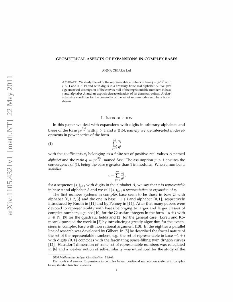
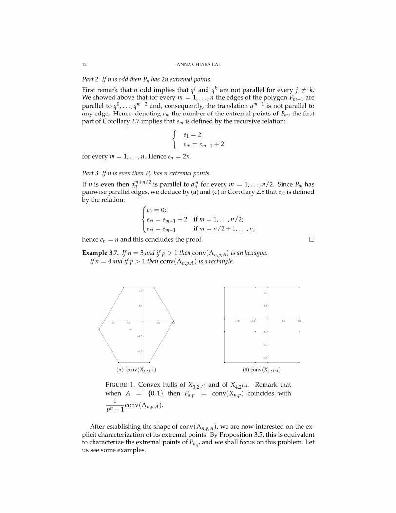
Example 3.7. If n = 3 and if p > 1 then conv(Λn,p,A) is an hexagon.If n = 4 and if p > 1 then conv(Λn,p,A) is a rectangle.

-1.0 -0.5 0.5 1.0

-1.0

-0.5

0.5

1.0

(A) conv(X3,21/3 )

-1.0 -0.5 0.5 1.0

-1.5

-1.0

-0.5

0.5

1.0

(B) conv(X4,21/4 )

FIGURE 1. Convex hulls of X3,21/3 and of X4,21/4 . Remark thatwhen A = {0, 1} then Pn,p = conv(Xn,p) coincides with

1pn − 1

conv(Λn,p,A).

After establishing the shape of conv(Λn,p,A), we are now interested on the ex-plicit characterization of its extremal points. By Proposition 3.5, this is equivalentto characterize the extremal points of Pn,p and we shall focus on this problem. Letus see some examples.


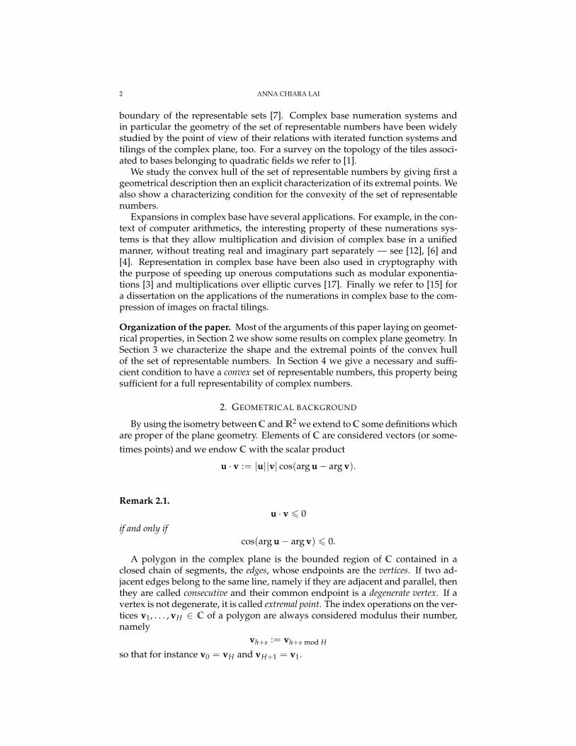
(A) n = 3 (B) n = 4 (C) n = 5

(D) n = 6 (E) n = 7 (F) n = 8

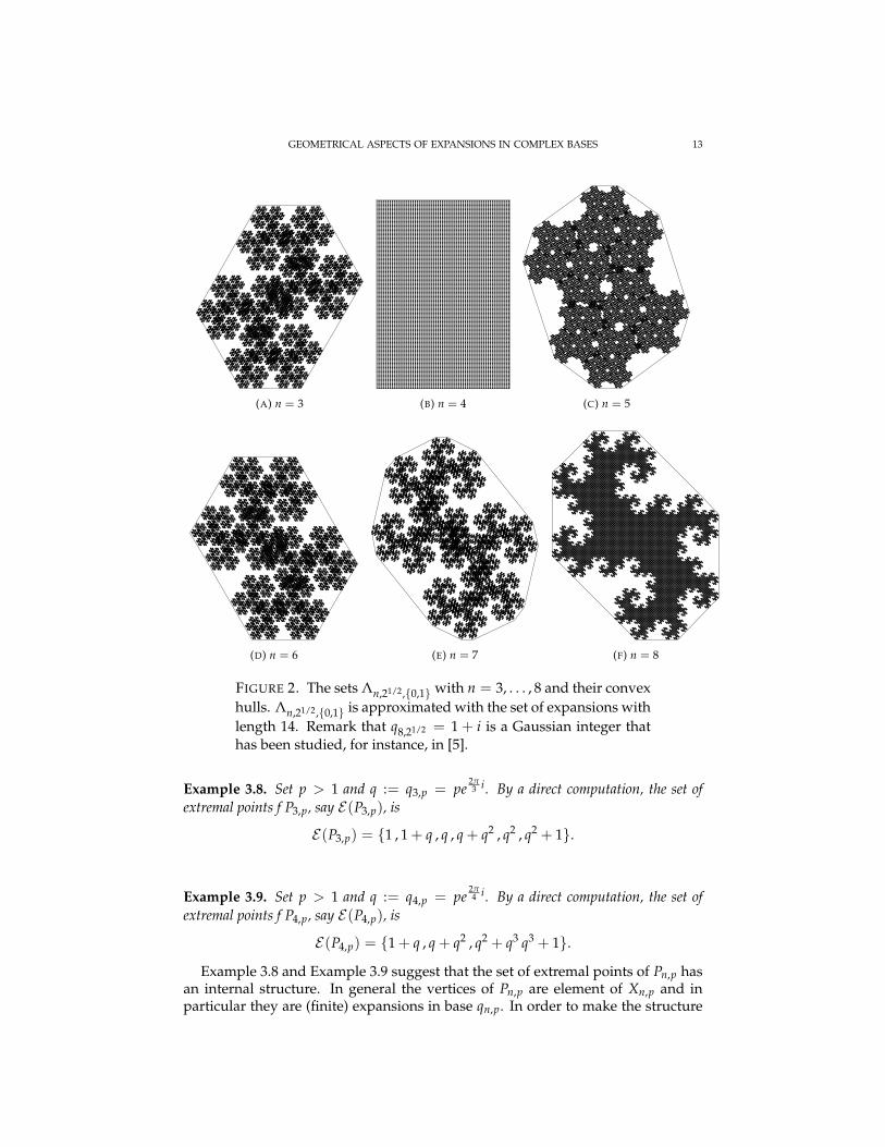
FIGURE 2. The sets Λn,21/2,{0,1} with n = 3, . . . , 8 and their convexhulls. Λn,21/2,{0,1} is approximated with the set of expansions withlength 14. Remark that q8,21/2 = 1 + i is a Gaussian integer thathas been studied, for instance, in [5].

Example 3.8. Set p > 1 and q := q3,p = pe2π3 i. By a direct computation, the set of

extremal points f P3,p, say E(P3,p), is

E(P3,p) = {1 , 1 + q , q , q + q2 , q2 , q2 + 1}.

Example 3.9. Set p > 1 and q := q4,p = pe2π4 i. By a direct computation, the set of

extremal points f P4,p, say E(P4,p), is

E(P4,p) = {1 + q , q + q2 , q2 + q3 q3 + 1}.

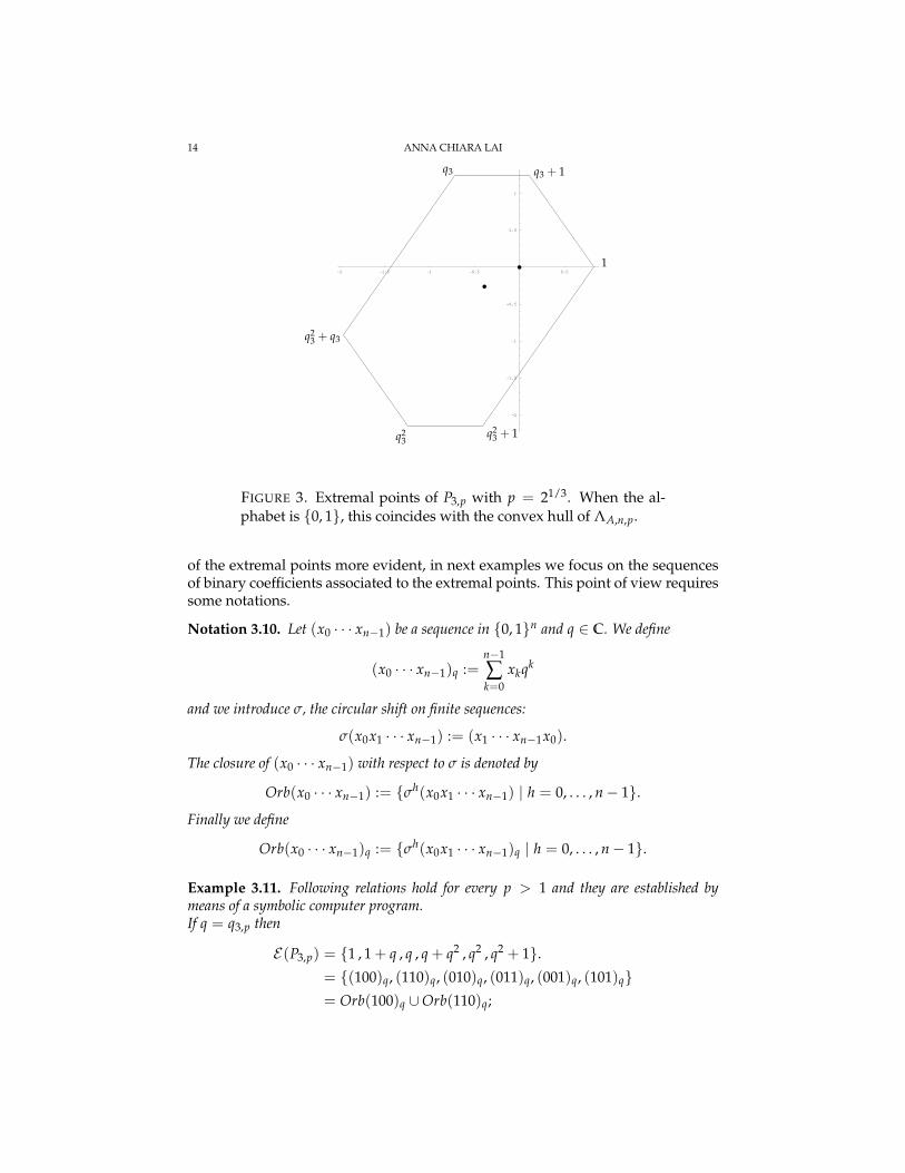
Example 3.8 and Example 3.9 suggest that the set of extremal points of Pn,p hasan internal structure. In general the vertices of Pn,p are element of Xn,p and inparticular they are (finite) expansions in base qn,p. In order to make the structure

14 ANNA CHIARA LAI

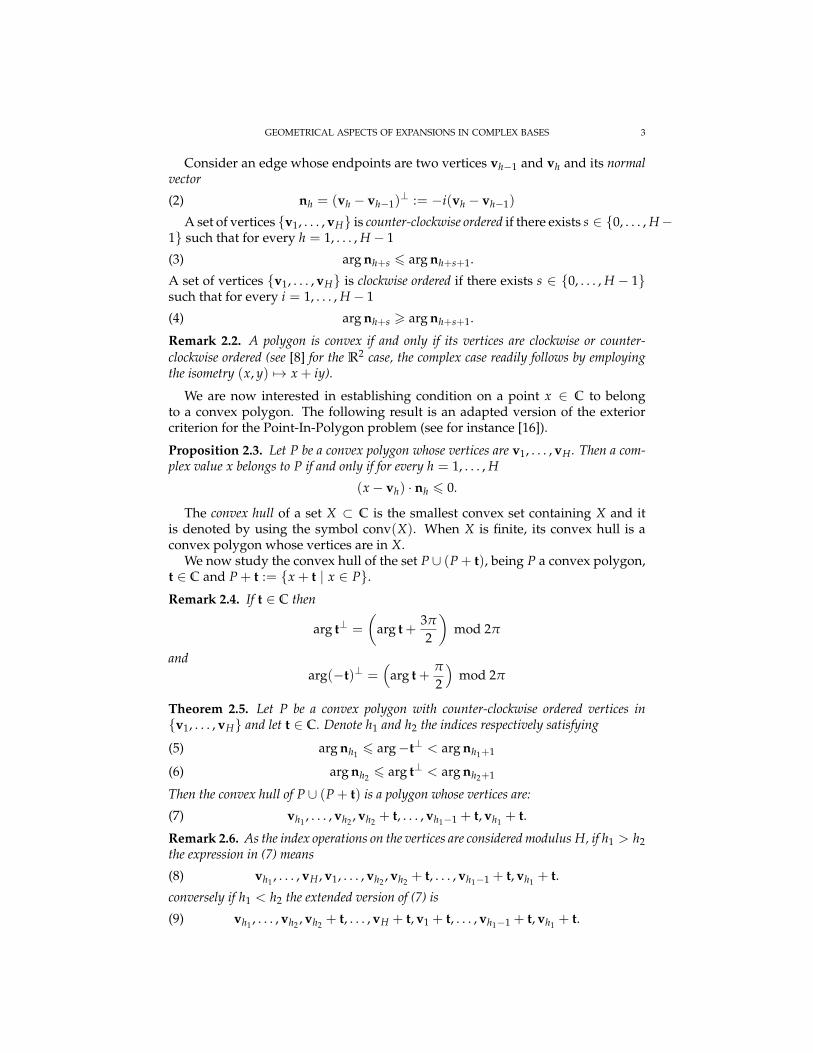
-2 -1.5 -1 -0.5 0.5

-2

-1.5

-1

-0.5

0.5

1

1

q3 + 1

q23 + 1

q3

q23 + q3

q23

FIGURE 3. Extremal points of P3,p with p = 21/3. When the al-phabet is {0, 1}, this coincides with the convex hull of ΛA,n,p.

of the extremal points more evident, in next examples we focus on the sequencesof binary coefficients associated to the extremal points. This point of view requiressome notations.

Notation 3.10. Let (x0 · · · xn−1) be a sequence in {0, 1}n and q ∈ C. We define

(x0 · · · xn−1)q :=n−1

∑k=0

xkqk

and we introduce σ, the circular shift on finite sequences:

σ(x0x1 · · · xn−1) := (x1 · · · xn−1x0).

The closure of (x0 · · · xn−1) with respect to σ is denoted by

Orb(x0 · · · xn−1) := {σh(x0x1 · · · xn−1) | h = 0, . . . , n− 1}.

Finally we define

Orb(x0 · · · xn−1)q := {σh(x0x1 · · · xn−1)q | h = 0, . . . , n− 1}.

Example 3.11. Following relations hold for every p > 1 and they are established bymeans of a symbolic computer program.If q = q3,p then

E(P3,p) = {1 , 1 + q , q , q + q2 , q2 , q2 + 1}.= {(100)q, (110)q, (010)q, (011)q, (001)q, (101)q}= Orb(100)q ∪Orb(110)q;


If q = q4,p then

E(P4.p) = {1 + q , q + q2 , q2 + q3 q3 + 1}.= {(1100)q, (0110)q, (0011)q, (1001)q}= Orb(1100)q;

If q = q5,p then

E(P5,p) = {(11000)q, (11100)q, (01100)q, (01110)q, (00110)q,

(00111)q, (00011)q, (10011)q, (10001)q, (11001)q}= Orb(1100)q ∪Orb(11100)q;

If q = q6,p then

E(P6,p) = {(111000)q, (011100)q, (001110)q,

(000111)q, (100011)q, (110001)q}= Orb(111000)q.

In Example 3.11 the set of extremal points E(Pn,p) is shown to be intimatelyrelated to the sequences (1bn/2c0n−bn/2c) and (1dn/2e0n−dn/2e) when n = 3, 5 andto the sequence (1n/20n/2) when n = 4, 6. We now prove that this is a generalresult. We set q = qn,p and for h = 1, . . . , n we introduce the vertices

v2h−1 := σh(1bn/2c0n−bn/2c) =bn/2c−1

∑k=0

qk+h−1 mod n(25)

= ∑k∈K(h)

qk(26)

where

K(h) := {k ∈ {0, . . . , n− 1} | (k− h + 1) mod n 6 bn/2c − 1};

v2h := σh(1dn/2e0n−dn/2e) =dn/2e−1

∑k=0

qk−h+1 mod n(27)

= ∑k∈K(h)

qk(28)

where

K(h) := {k ∈ {0, . . . , n− 1} | (k− h + 1) mod n 6 dn/2e − 1}.

Remark 3.12. By a direct computation, if n is odd then for every h = 1, . . . , n

n2h−1 = (−qh−2 mod n)⊥(29)

n2h = (qh−2+dn/2e mod n)⊥(30)

while if n is even then v2h = v2h−1 hence

n2h−1 =

(1− 1

pn/2

)(−qh−2 mod n)⊥(31)

n2h = 0;(32)

16 ANNA CHIARA LAI

In view of (29) and of (31), for every n and every h

(33) arg n2h−1 =

((h− 2) mod n

n2π +

π

2

)mod 2π

Lemma 3.13. For every h = 1, . . . , n

(34) k ∈ K(h) if and only if qk · n2h−1 > 0;

(35) k ∈ K(h) if and only if qk · n2h > 0;

Proof. For every k = 0, . . . , n− 1

(36) qk · n2h−1 > 0

if and only if

(37) cos(

arg qk − arg n2h−1

)= cos

((k− h + 1) mod n + 1

n2π − π

2

)> 0

As (k− h + 1) mod n ∈ {0, . . . , n− 1},

−π

2<

(k− h + 1) mod n + 1n

2π − π

26

3π

2,

(37) reduces to

−π

2<

(k− h + 1) mod n + 1n

2π − π

26

π

2Hence (34) follows by the definition of k ∈ K(h) and by recalling that (k − h +1) mod n ∈N.

To prove (35), we first remark that if n is even then n2h = 0 and (35) is immedi-ate. If otherwise n is odd then

arg n2h =

((h− 2 + dn/2e) mod n

n2π +

3π

2

)mod 2π

therefore

(38) qk · n2h−1 > 0

if and only if

(39) cos((k− h + 1) mod n + 1− dn/2e

n2π +

π

2

)> 0.

As (k− h + 1) mod n ∈ {0, . . . , n− 1}, for every k = 0, . . . , n− 1

−π

2<

(k− h + 1) mod n + 1n

2π − π

26

3π

2,

(37) reduces to

−π

2<

(k− h + 1) mod n + 1n

2π − π

26

π

2;

Relation (35) hence follows by the definition of K(h). �


Lemma 3.14. For every x ∈ Xn,p and for every h = 1, . . . , n

(40) (x− v2h−1) · n2h−1 6 0

and

(41) (x− v2h) · n2h 6 0.

Proof. Let

x =n−1

∑k=0

xkqk ∈ Xn,p

with x0, . . . , xn−1 ∈ {0, 1}. Then for every h = 1, . . . , n

(x− v2h−1) · n2h−1 = ∑k∈K(h)

(xk − 1)(qk · n2h−1) + ∑k 6∈K(h)

xk(qk · n2h−1) 6 0

indeed Lemma 3.13 and xk ∈ {0, 1} imply that all the terms of the above sums arenon-positive. Similarly, again by Lemma 3.13 and by xk ∈ {0, 1} we may deduce

(x− v2h−1) · n2h−1 = ∑k∈K(h)

(xk − 1)(qk · n2h−1) + ∑k 6∈K(h)

xk(qk · n2h−1) 6 0.

�

Remark 3.15. Proposition 2.3 and Lemma 3.14 imply that Xn,p is a subset of the polygonwhose vertices are v1, . . . v2n, therefore

Pn,p = conv(Xn,p) ⊆ conv{vh | h = 1, . . . , n}.

This, together with the fact that vh ∈ Xn,p for every h = 1, . . . , 2n, implies

(42) Pn,p = conv({vh | h = 1, . . . , 2n}).

In particular when n is odd v1, . . . , v2n coincide with the 2n vertices of Pn,p. When n iseven, v1 = v2, . . . , v2n−1 = v2n are the n vertices of Pn,p.

Theorem 3.16. For every n > 1, p > 1 and for every finite alphabet A


pn − 1conv({vh | h = 1, . . . , 2n}) +

n−1

∑k=0

min A qk.

Moreover if n is even then


pn − 1conv({v2h | h = 1, . . . , n}) +

n−1

∑k=0

min A qk.

Proof. In view of Remark 3.15, (43) immediately follows by Proposition 3.5. while(44) holds because if n is even then v2h = v2h−1 for every h = 1, . . . , n. �

18 ANNA CHIARA LAI

4. REPRESENTABILITY IN COMPLEX BASE

In this section we give a characterization of the convexity of Λn,p,A. To this endwe recall some basic elements of the Iterated Function System (IFS) theory. An IFSF is a finite set of contractive maps over a metric space X, in particular if X = C

thenF = { fi : C→ C|i = 1, . . . , m}

for some m ∈N and for every x, y ∈ C and i = 1, . . . , m

| fi(x)− fi(y)| 6 ci|x− y|for some 0 < ci < 1. The Hutchinson operator acts on the power set of C as follows

F (X) :=m⋃

i=1

fi(X) =m⋃

i=1

⋃x∈X

fi(x).

By the contraction principle, every IFS has a unique fixed point R = F (R) that canbe constructed starting by any subset of C, indeed for every X ⊂ C

R = limk→∞F k(X).

Example 4.1. If q ∈ C and if |q| > 1 then

F =

{fi : x 7→ 1

q(x + ai) | ai ∈ R; i = 1, . . . , m

}is an IFS.

We define

(45) Fq,A :={

fi : x 7→ 1q(x + ai) | ai ∈ A

}.

Lemma 4.2. Let q ∈ C, |q| > 1 and A = {a1, . . . , am} ⊂ R. Then the fixed point ofFq,A is

Λq,A :=

{∞

∑k=1

xk

qk | xk ∈ A

}.

Proof. For every

x =∞

∑k=1

xk

qk ∈ Λq,A

we have

fi(x) =1q

x +1q

ai =∞

∑i=2

xk−1

qk +aiq∈ Λq,A.

Moreover if x1 = ai then

f−1i (x) = qx− ai = x1 + q

∞

∑k=2

xk

qk − ai =∞

∑k=1

xk+1

qi ∈ Λn,p,A.

Thereforem⋃

i=1

fi(Λq,A) = Λq,A

namely Λn,p,A is the fixed point of Fq,A. �


(A) (B) (C)

(D) (E) (F)

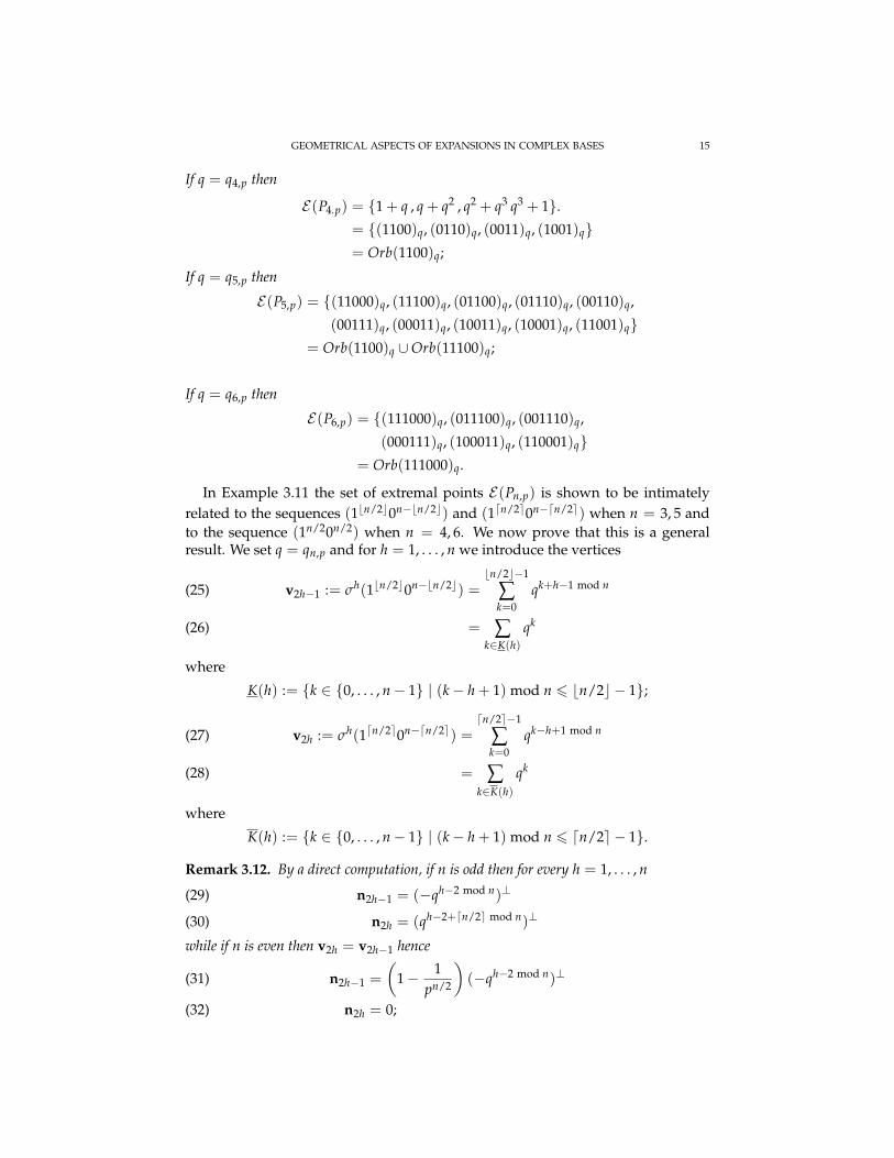
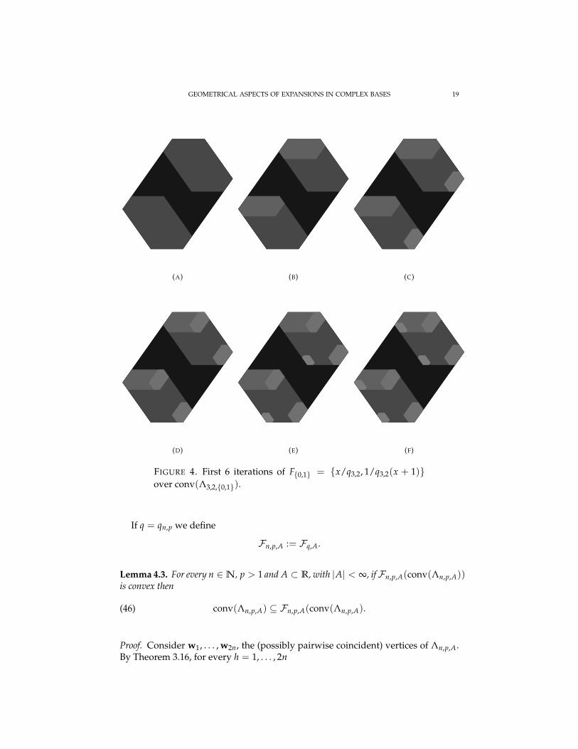
FIGURE 4. First 6 iterations of F{0,1} = {x/q3,2, 1/q3,2(x + 1)}over conv(Λ3,2,{0,1}).

If q = qn,p we define

Fn,p,A := Fq,A.

Lemma 4.3. For every n ∈N, p > 1 and A ⊂ R, with |A| < ∞, ifFn,p,A(conv(Λn,p,A))is convex then

(46) conv(Λn,p,A) ⊆ Fn,p,A(conv(Λn,p,A).

Proof. Consider w1, . . . , w2n, the (possibly pairwise coincident) vertices of Λn,p,A.By Theorem 3.16, for every h = 1, . . . , 2n

20 ANNA CHIARA LAI

wh =max A−min A

pn − 1vh +

1pn − 1

n−1

∑k=0

min A qk

=max A−min A

pn − 1σh(1l0n−l)q +

1pn − 1

n−1

∑k=0

min A qk

for some h ∈ {1, . . . , n} and l ∈ {bn/2c, dn/2d}. Remark that if ε ∈ {0, 1} is thelast digit of σh(1l0n−1) then

qσh(1l0n−l)q = σh+1(1l0n−l)q + ε(1− qn).

Now, as qn = pn if ε = 0 then

f−11 (wh) = qwh −min A

=max A−min A

pn − 1(qσh(1l0n−l)q) +

qpn − 1

n−1

∑k=0

min A qk −min A

=max A−min A

pn − 1(σh+1(1l0n−l)q) +

1pn − 1

n−1

∑k=0

min A qk

= wh+2.

therefore f1(wh+2) = wh. By a similar argument, it is possible to show that if ε = 1then fm(wh+2) = wh. Thus

(47) wh ∈ Fq,A({wh | h = 1, . . . , 2n}

and, by the arbitrariness of wh,

(48) {wh | h = 1, . . . , 2n} ⊆ Fq,A({wh | h = 1, . . . , 2n}

Hence

conv(Λn,p,A) =conv({wh | h = 1, . . . , 2n})⊆conv

(Fq,A({wh | h = 1, . . . , 2n})

)=conv

(m⋃

i=1

fi({wh | h = 1, . . . , 2n}))

⊆conv

(m⋃

i=1

fi(conv({wh | h = 1, . . . , 2n})))

=conv(Fn,p,A(conv(Λn,p,A)))

=Fn,p,A(conv(Λn,p,A)).

�

Lemma 4.4. For every n ∈N, p > 1 and A ⊂ R

(49) Fn,p,A(conv(Λn,p,A)) ⊆ conv(Λn,p,A).


Proof. Let y ∈ Fn,p,A(conv(Λn,p,A)) so that y = fi(x) for some i = 1, . . . , m andsome x ∈ conv(Λn,p,A). In particular x = αx1 + (1− α)x2 for some x1, x2 ∈ Λn,p,Aand, consequently,

y = α fi(x1) + (1− α) fi(x2)

because fi is a linear map. Since Λn,p,q is the fixed point of an IFS containing fi wehave fi(x1), fi(x2) ∈ Λn,p,A and, consequently, y ∈ conv(Λn,p,A). Thesis followsby the arbitrariness of y. �

Lemma 4.5. For every n ∈ N, p > 1 and A ⊂ R, Λn,p,A is convex if and only ifFn,p,A(conv(Λn,p,A)) is convex.

Proof. If Λn,p,A is convex, then the convexity of Fn,p,A(conv(Λn,p,A)) follows by

(50) conv(Λn,p,A) = Λn,p,A = Fn,p,A(Λn,p,A) = Fn,p,A(conv(Λn,p,A)).

If otherwise Fn,p,A(conv(Λn,p,A)) is convex, then by Lemma 4.3

conv(Λn,p,A) ⊆ Fn,p,A(conv(Λn,p,A))

while Lemma 4.4 implies

Fn,p,A(conv(Λn,p,A)) ⊆ conv(Λn,p,A);

thereforeFn,p,A(conv(Λn,p,A)) = conv(Λn,p,A);

and by the uniqueness of the fixed point of Fn,p,A

conv(Λn,p,A) = Λn,p,A.

�

Theorem 4.6. The set of representable numbers in base qn,p and alphabet A = {ai | i =1, . . . , m} is convex if and only if

(51) maxi=1,...,m−1

ai+1 − ai 6max A−min A

pn − 1.

Proof. By applying Proposition 2.9 with P = Pn,p and

ti = aipn − 1

max A−min A,

we get that (51) holds if and only ifm⋃

i=1

(Pn,p + ti)

is convex. Then (51) is equivalent to the convexity of

P :=max A−min A

q(pn − 1)

m⋃i=1

(Pn,p + ti) +1

q(pn − 1)

n−1

∑k=0

min A qk.

=m⋃

i=1

1q

(max A−min A

q(pn − 1)Pn,p +

1q(pn − 1)

n−1

∑k=0

min A qk + ai

)

22 ANNA CHIARA LAI

(A) Λ3,21/3 ,{0,1} (B) Λ3,21/3+0.1,{0,1} (C) Λ3,21/3+0.2,{0,1}

(D) Λ3,21/3+0.3,{0,1} (E) Λ3,21/3+0.4,{0,1} (F) Λ3,21/3+0.5,{0,1}

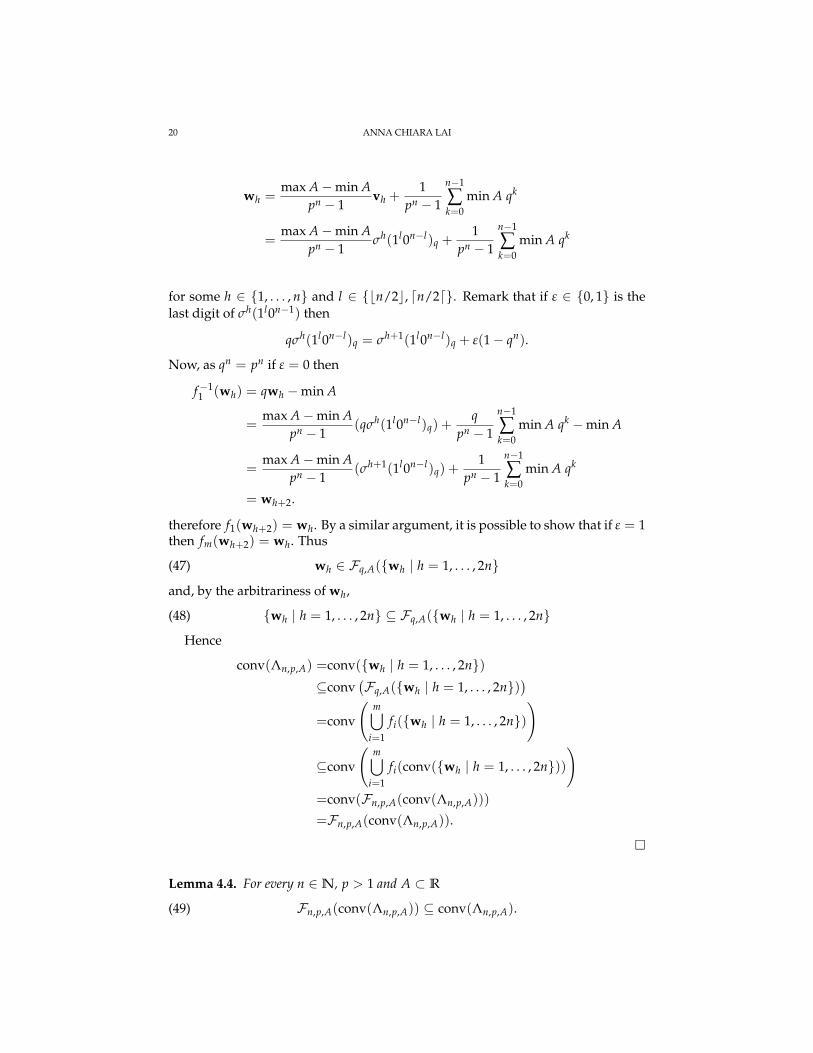
FIGURE 5. Λ3,21/3+0.1k,{0,1}, with k = 0, . . . , 5, is approximatedwith the set of expansions with length 14.

By Theorem 3.16 we have

P =m⋃

i=1

1q(conv(Λn,p,A) + ai

)= Fn,p,A(conv(Λn,p,A)),

therefore Fn,p,A(conv(Λn,p,A)) is convex if and only if (51) holds. Thesis hencefollows by Lemma 4.5. �

Corollary 4.7. Let A = {ai | i = 1, . . . , m}. If

maxi=1,...,m−1

ai+1 − ai 6max A−min A

pn − 1

then every

x ∈ max A−min Apn − 1

Pn,p +n−1

∑k=0

min Aqkn,p

has a representation in base qn,p and alphabet A.


Proof. It immediately follows by Theorem 4.6. �

Example 4.8. If p = 21/n and A = {0, 1} then Λn,p,A is a convex set coinciding withPn,p. In particular Λn,p,A is an 2n-gon if n is odd and it is an n-gon if n is even.

Example 4.9. If A = {0, 1, . . . , bpnc} then Λn,p,A is a convex set or, equivalently,

bpncpn − 1

Pn,p

is completely representable.

REFERENCES

[1] S. Akiyama and J. M. Thuswaldner. A survey on topological properties of tiles related to numbersystems. Geom. Dedicata, 109:89–105, 2004.

[2] Z. Daroczy and I. Katai. Generalized number systems in the complex plane. Acta Math. Hungar.,51(3-4):409–416, 1988.

[3] V. A. Dimitrov, G. A. Jullien, and Miller W.C. Complexity and fast algorithms for multiexponenti-ation. 31:141–147, 1985.

[4] Ch. Frougny and A. Surarerks. On-line multiplication in real and complex base. Computer Arith-metic, IEEE Symposium on, 0:212, 2003.

[5] W. J. Gilbert. Geometry of radix representations. In The geometric vein, pages 129–139. Springer,New York, 1981.

[6] W. J. Gilbert. Arithmetic in complex bases. Math. Mag., 57(2):77–81, 1984.[7] W. J. Gilbert. Complex bases and fractal similarity. Ann. Sci. Math. Quebec, 11(1):65–77, 1987.[8] editor Heckbert, P. S. Graphics Gems IV. Academic Press, 1994.[9] I. Katai and B. Kovacs. Canonical number systems in imaginary quadratic fields. Acta Math. Acad.

Sci. Hungar., 37(1-3):159–164, 1981.[10] I. Katai and J. Szabo. Canonical number systems for complex integers. Acta Sci. Math. (Szeged),

37(3-4):255–260, 1975.[11] D. E. Knuth. An imaginary number system. Comm. ACM, 3:245–247, 1960.[12] D. E. Knuth. The art of computer programming. Vol. 2. Addison-Wesley Publishing Co., Reading,

Mass., first edition, 1971. Seminumerical algorithms, Addison-Wesley Series in Computer Scienceand Information Processing.

[13] V. Komornik and P. Loreti. Expansions in complex bases. Canad. Math. Bull., 50(3):399–408, 2007.[14] W. Penney. A “binary” system for complex numbers. J. ACM, 12(2):247–248, 1965.[15] D. Piche. Complex bases, number systems and their application to the fractal wavelet image cod-

ing. PhD thesis (Univ. Waterloo, Ontario, 0, 2002.[16] J. Pineda. A parallel algorithm for polygon rasterization. 22(4):17–20, 1988.[17] J. A. Solinas. Efficient arithmetic on Koblitz curves. Des. Codes Cryptogr., 19(2-3):195–249, 2000.

Towards a quarter-century of public key cryptography.

DIPARTIMENTO DI SCIENZE DI BASE E APPLICATE PER L’INGEGNERIA, SAPIENZA UNIVERSITA DI

ROMA

Geometrical aspects of expansions in complex bases

Documents