Geometric Path-Planning Algorithm in Cluttered 2D ...

Clemson UniversityTigerPrints

All Theses Theses

12-2017

Geometric Path-Planning Algorithm in Cluttered2D Environments Using Convex HullsNafiseh MasoudiClemson University

Follow this and additional works at: https://tigerprints.clemson.edu/all_theses

This Thesis is brought to you for free and open access by the Theses at TigerPrints. It has been accepted for inclusion in All Theses by an authorizedadministrator of TigerPrints. For more information, please contact [email protected].

Recommended CitationMasoudi, Nafiseh, "Geometric Path-Planning Algorithm in Cluttered 2D Environments Using Convex Hulls" (2017). All Theses. 2784.https://tigerprints.clemson.edu/all_theses/2784

https://tigerprints.clemson.edu?utm_source=tigerprints.clemson.edu%2Fall_theses%2F2784&utm_medium=PDF&utm_campaign=PDFCoverPages

https://tigerprints.clemson.edu/all_theses?utm_source=tigerprints.clemson.edu%2Fall_theses%2F2784&utm_medium=PDF&utm_campaign=PDFCoverPages

https://tigerprints.clemson.edu/theses?utm_source=tigerprints.clemson.edu%2Fall_theses%2F2784&utm_medium=PDF&utm_campaign=PDFCoverPages

https://tigerprints.clemson.edu/all_theses?utm_source=tigerprints.clemson.edu%2Fall_theses%2F2784&utm_medium=PDF&utm_campaign=PDFCoverPages

https://tigerprints.clemson.edu/all_theses/2784?utm_source=tigerprints.clemson.edu%2Fall_theses%2F2784&utm_medium=PDF&utm_campaign=PDFCoverPages

mailto:[email protected]

GEOMETRIC PATH-PLANNING ALGORITHM IN CLUTTERED 2D ENVIRONMENTSUSING CONVEX HULLS

A Thesis

Presented to

the Graduate School of

Clemson University

In Partial Fulfillment

of the Requirements for the Degree

Master of Science

Mechanical Engineering

by

Nafiseh Masoudi

December 2017

Accepted by:

Dr. Georges Fadel, Committee Chair

Dr. Margaret Wiecek, Co-Chair

Dr. Joshua D. Summers

Dr. Gang Li

http://www.ces.clemson.edu/~agramop/

ii

ABSTRACT

Routing or path planning is the problem of finding a collision-free path in an

environment usually scattered with multiple objects. Finding the shortest route in a planar

(2D) or spatial (3D) environment has a variety of applications such as robot motion

planning, navigating autonomous vehicles, routing of cables, wires, and harnesses in

vehicles, routing of pipes in chemical process plants, etc. The problem often times is

decomposed into two main sub-problems: modeling and representation of the workspace

geometrically and optimization of the path. Geometric modeling and representation of the

workspace is paramount in any path planning problem since it builds the data structures

and provides the means for solving the optimization problem. The optimization aspect of

the path planning involves satisfying some constraints, the most important of which is to

avoid intersections with the interior of any object, and optimizing one or more criteria. The

most common criterion in path planning problems is to minimize the length of the path

between a source and a destination point of the workspace while other criteria such as

minimizing the number of links or curves could also be taken into account.

Planar path planning is mainly about modeling the workspace of the problem as a

collision free graph. The graph is later on searched for the optimal path using network

optimization techniques such as branch-and-bound or search algorithms such as Dijkstra’s.

Previous methods developed to construct the collision free graph explore the entire

workspace of the problem which usually results in some unnecessary information that has

no value but to increase the time complexity of the algorithm, hence, affecting the

efficiency significantly. For example, the fastest known algorithm to construct the visibility

iii

graph, which is the most common method of modeling the collision free space, in a

workspace with a total of n vertices has a time complexity of order O(n2).

In this research, first, the 2D workspace of the problem is modeled using the

tessellated format of the objects in a CAD software which facilitates handling of any free

form object. Then, an algorithm is developed to construct the collision free graph of the

workspace using the convex hulls of the intersecting obstacles. The proposed algorithm

focuses only on a portion of the workspace involved in the straight line connecting the

source and destination points. Considering the worst case that all the objects of the

workspace are intersecting, the algorithm yields a time complexity of O(nlog(n/f)), with n

being the total number of vertices and f being the number of objects. The collision free

graph is later searched for the shortest path between the two given nodes using a search

algorithm known as Dijkstra’s.

iv

TABLE OF CONTENTS

Abstract ............................................................................................................................ ii List of Tables...................................................................................................................vi

Nomenclature ...................................................................................................................ix

Chapter One Introduction .............................................................................................. 10

1.1 Objectives of this Research ................................................................................. 18

Chapter Two literature review ....................................................................................... 20

2.1 State of the art in Roadmap techniques ............................................................... 20

2.2 3D shortest path problem ..................................................................................... 29

2.3 Research Questions .............................................................................................. 34

Chapter Three geometric Representation....................................................................... 35

3.1 Geometric Representation Schemes .................................................................... 35

3.2 Tessellated Representation .................................................................................. 37

3.3 Data Structures ..................................................................................................... 44

Chapter Four intersection Detection .............................................................................. 48

4.1 State-of-the-art in Interference Detection ............................................................ 48

4.2 Bi-level Collision Detector .................................................................................. 49

Chapter Five Development of the free-space graph ...................................................... 66

5.1 Existing Techniques ............................................................................................. 67

5.2 Proposed Approach: Planning based on the convex hulls of the

obstacles ............................................................................................................... 72

Chapter Six Path Optimization ...................................................................................... 88

6.1 Formulation of the network optimization problem .............................................. 88

6.2 Dijkstra’s Shortest Path Algorithm ...................................................................... 90

6.3 A* Search Algorithm ........................................................................................... 96

Chapter Seven validation and time complexity of the algorithm ................................ 100

7.1 Time Complexity of the C-Hull Based Roadmap .............................................. 101

List of Figures .................................................................................................................vii

Title Page........................................................................................................................... i

v

7.2 Validation ........................................................................................................... 102

Chapter Eight conclusions and future work ................................................................. 104

8.1 Future Work ....................................................................................................... 108

appendix A ................................................................................................................... 113

appendix B ................................................................................................................... 130

References .................................................................................................................... 153

vi

LIST OF TABLES

Table 2.1 Shortcomings of Geometric Path Planning Approaches................................ 32

Table 4.1: Y-Coordinate Values of Object 6 ............................................................. 56

Table 4.2: Different Cases of Intersections in a Planar

Workspace .............................................................................................................. 63

Table 5.1: free-space Graphs of Different Sample Workspaces .............................. 84

Table 6.1: Mathematical Model of the Network Optimization

Problem ................................................................................................................... 89

Table 6.2: Dijkstra’s algorithm pseudo code ............................................................. 91

Table 7.1: Time Complexity of the Roadmap Algorithms ..................................... 100

Table A.1 Test Results of the Effects of the Number of Objects and

Intersections ........................................................................................................... 121

Table A.2 Effects of the Workspace Density............................................................... 126

Table A.3 Effects of Increasing the Number of Vertices per Object ........................... 127

vii

LIST OF FIGURES

Figure 1.1 Path Planning Problem Domains .................................................................. 13

Figure 3.1: Sample Solid Model of a Workspace ...................................................... 36

Figure 3.2: Tessellated Under-hood Components ..................................................... 37

Figure 3.3: Sample STL File of a Workspace in ASCII Format ............................. 38

Figure 3.4: Shared edge of a triangulated solid ........................................................ 39

Figure 3.5: Closure Error in an STL Tessellated Solid

Model[40] ................................................................................................................ 39

Figure 3.6: Sample VRML File of a Workspace in ASCII

Format ..................................................................................................................... 40

Figure 3.7: Sample Tessellated 2D Workspace Imported in

MATLAB ................................................................................................................ 42

Figure 3.8: Planar Workspace after the Elimination of the

Interior Edges ......................................................................................................... 43

Figure 3.9: Multidimensional Cell Array[42] ............................................................ 45

Figure 4.1: Transformation of the Coordinate System ............................................ 52

Figure 4.2: Minimum Bounding Box (MBB) of a Polygon ...................................... 53

Figure 4.3: Example of a Polygon Lying at One Side of the

Line .......................................................................................................................... 54

Figure 4.4: Example of an Intersecting Polygon ....................................................... 55

Figure 4.5: Flowchart of the Bi-level Collision Detector

Algorithm ................................................................................................................ 57

Figure 4.6: Non-intersecting Polygon with Collision Possibility ............................. 58

Figure 4.7: Non-intersecting Obstacles ...................................................................... 60

Figure 4.8: Intersecting Obstacle................................................................................ 60

Figure 5.1: Sample Visibility Graph .......................................................................... 68

Figure 5.2: Visibility Graph of a Nonconvex Polygon .............................................. 69

Figure 5.3: Example of a Voronoi Diagram of Four

Obstacles[27] .......................................................................................................... 70

Figure 5.4: Line segment and polygon intersection .................................................. 75

Figure 5.5: Ordering the Intersecting Obstacles ....................................................... 77

Figure 5.6: Extreme Points of a Convex Hull ............................................................ 78

viii

Figure 5.7: Schematic of the First Iteration in Construction of

the Free Space Graph ............................................................................................ 79

Figure 5.8: Free Space Graph Of The Figure 5.5 Workspace ................................. 80

Figure 5.9: Flowchart of the free-space graph construction .................................... 83

Figure 5.10: Start Point (2003) Lying inside the Convex Hull ................................. 86

Figure 5.11: Free Space Graph Using Backtracking ................................................ 87

Figure 6.1: Dijkstra’s Initialization ............................................................................ 92

Figure 6.2: Dijkstra’s First Iteration ......................................................................... 93

Figure 6.3: Dijkstra’s Second Iteration ..................................................................... 93

Figure 6.4: Dijkstra’s Third Iteration ........................................................................ 94

Figure 6.5: Dijkstra’s Shortest Path Solution ........................................................... 95

Figure 6.6: Shortest Path Found on a Graph Using Dijkstra .................................. 96

Figure 6.7: Finding the Shortest Path ........................................................................ 98

Figure 6.8: Shortest Path on the graph of Figure 5.8 ............................................... 99

Figure 8.1: Sample Planar Workspace .................................................................... 106

Figure 8.2: Free Space Graph for Pair (61, 73) ....................................................... 106

Figure 8.3: Free Space Graph for Pair (82, 53) ....................................................... 107

Figure 8.4: Superposition of Two Free Space Graphs for Pairs

(61, 73) and (82, 53) .............................................................................................. 107

ix

NOMENCLATURE

C-hull Convex hull

E Set of edges of a graph

f Total number of obstacles in the workspace

L Total number of links or line segments in a workspace

m Number of intersecting obstacles

n Total number of vertices in a workspace

N Total number of facilities in the facility location problem

nave Average number of vertices per object

nmax Maximum number of vertices per object

P Polygon or set of disjoint polygons

V Set of vertices of a graph

10

Chapter One

INTRODUCTION

In today’s highly competitive business environment, industries strive to develop

smaller and lighter products while increasing their performance. One critical issue is how

to assemble the required subcomponents in tighter enclosures while ensuring ease of

assembly and full functionality. Compact packaging of a finite number of components in

an enclosed domain is an example of such assembly planning for smaller systems.

In an attempt to design a compact package, Dandurand et. al. [1] formulate the

problem of designing a layout for hybrid vehicles as a bi-level optimization problem. In

their article, the compact packaging of components in vehicle under-hood to achieve an

optimum center of gravity, accessibility, survivability, dynamic behavior, and other

objectives is undertaken. Before Dandurand, other research studies have been done on

addressing different types of packaging problem. for example, Wodziak and Fadel [2],

propose a methodology based on the Genetic Algorithm (GA), a heuristic optimization

technique, to solve the optimal packing of rectangular boxes in a rectangular shaped

enclosure. The objective of this optimization problem is to find the optimal location for the

center of gravity of the system. In a separate study, Grignon and Fadel [3], take more

complex shapes (including non-convex and hollow shapes) into account in the packaging

problem and find the optimal configuration for a system of components (based on their

locations) using GA. The objectives of this optimization problem, in addition to the

location of the center of gravity (balance), are compactness and maintainability, hence,

making the problem multi-criteria. Furthermore, in all packaging problems, the most

11

important constraint is to avoid any interference between the components to be packed. In

view of multiple objective packaging problem, Miao et.al. [4] use Multiple Objective

Genetic Algorithm (MOGA) to optimize the configuration based on the ground clearance

and dynamic behavior and apply the method to the design of a midsize truck. For the

multiple criteria optimization problems, since the criteria are in conflict, the solution will

be a Pareto front (rather than a single point in the domain) and a solution can be selected

based on a trade-off between the criteria. As a new solution method to the packaging

problem, Dong et.al. [5] propose using the rubber band analogy. Their method simulates

the movement of the components based on the elastic force of the rubber band (2D) or

rubber balloon (3D) and a reaction force by the components to avoid collisions between

them. Following this approach, they are able to find the locations of the components such

that the maximum compactness is achieved. Tiwari et.al.[6] move on to a step further and

propose a GA-based optimization algorithm to find both the compact packing and the

sequence of packing a set of 3D free form components inside an arbitrary enclosure. Finally

from a different perspective, Katragadda et.al. [7] investigate the thermal performance of

a vehicle under-hood packaging optimization. Hence, in addition to the packaging

optimization criteria of minimizing the height of the center of gravity and maximizing the

accessibility and survivability, they include the thermal performance of the vehicle under-

hood. Exploitation of a CFD analysis, leads them to the temperatures of various

components under different configurations. Finally, an optimizer identifies optimal

configuration based on the lower thermal risk for the components.

12

After the identification of an optimal way to pack components and devices under

the hood, the problem of how to connect them efficiently arises; this is the wire, hose or

pipe routing problem.

Wires or cables and hoses or pipes are used in every electro-mechanical system to

connect subsystems and components. For example, under the hood of an automobile or in

ships and aircraft engines, hundreds to thousands of wires, hoses, and pipes are used,

adding significant weight to the system. Wires are often times bundled together in cable

harnesses for protection and ease of assembly. As new features are continuously added to

the vehicles, their cable harnesses are becoming heavier and more complex to design.

According to Matheus in his book “Automotive Ethernet” [8], cabling is the third heaviest

and costliest component in a car after its engine and chassis. Therefore, an optimal cable

and hose routing is required to reduce their length and therefore minimize the total weight

of a vehicle while at the same time directly impacting fuel efficiency.

Traditionally, cables and hoses have been routed using a manual trial-and-error

approach in a CAD system. It was sometimes tested on prototypes, but it is mostly based

on the experience of the skilled engineers. This manual approach is time-consuming,

tedious, and error-prone. In addition, most of the time, it results in suboptimal solutions.

Automating the optimal routing of these cables and hoses has been a challenging question

for decades.

Routing or path planning, the problem of finding the shortest collision-free path in

an environment (e.g. a graph or a geometric space), appears not only in the vehicle

assembly planning but also in other disciplines including pipe routing in chemical process

13

plants, robot motion planning, navigating autonomous vehicles, routing on networks, and

so on. In all these instances there are some criteria (e.g., minimization of the length of the

path) to be optimized and constraints to be satisfied (such as collision avoidance). These

constraints and criteria could differ depending on the discipline and problem specifics.

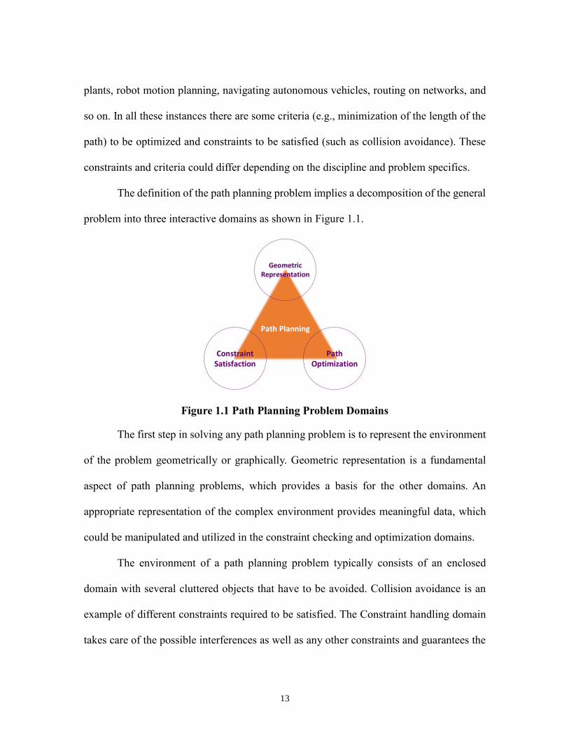
The definition of the path planning problem implies a decomposition of the general

problem into three interactive domains as shown in Figure 1.1.

Path Planning

Path Optimization

Constraint Satisfaction

Geometric Representation

Figure 1.1 Path Planning Problem Domains

The first step in solving any path planning problem is to represent the environment

of the problem geometrically or graphically. Geometric representation is a fundamental

aspect of path planning problems, which provides a basis for the other domains. An

appropriate representation of the complex environment provides meaningful data, which

could be manipulated and utilized in the constraint checking and optimization domains.

The environment of a path planning problem typically consists of an enclosed

domain with several cluttered objects that have to be avoided. Collision avoidance is an

example of different constraints required to be satisfied. The Constraint handling domain

takes care of the possible interferences as well as any other constraints and guarantees the

14

feasibility of the path. Path planning on networks and graphs is not concerned with the

collision avoidance constraint and this type of constraint is only critical in problems dealing

with geometric environments cluttered with obstacles.

The Path optimization domain deals with solving a routing problem. Some of the

optimization objectives include the length of the path (e.g., Euclidian length), number of

turns in the path, the sharpness of the turns, and time to complete the path.

The Path planning problem could occur in any n-dimensional space. The addition

of one dimension to the problem would significantly affect the computational complexity

of the problem. Therefore, it is reasonable to start solving the path planning problem in

lower dimensions and after testing different cases and validating the solutions, adapt the

approach to the higher dimensions.

The 2D path planning problem is the simplest case of a routing problem which

mainly involves finding the shortest path on the graph of the collision-free space. In order

to satisfy the collision avoidance constraint in 2D geometric workspaces cluttered with

obstacles, the problem is converted to constructing a network or graph from the free space

and searching that graph for the optimal solution. The free space is the region of the

workspace not occupied by any of the obstacles.

Path planning on networks for transportation and communication problems is an

example of the 2D planning in which there usually exists a known set of nodes and

segments that connect those nodes forming a graph. For example, the nodes could represent

cities (locations of supply and demand) and the segments represent the flow of goods,

information or signal between the two nodes.

15

A well-known and most-studied example of graph routing is the Travelling

Salesman Problem. In this problem, a salesperson travels to a known set of cities

represented as nodes. S/he has to visit each city exactly once and return to the starting point.

The criterion is to minimize the total travel distance. This problem is known to be NP-hard,

which means it cannot be solved using deterministic optimization techniques in polynomial

time [7].

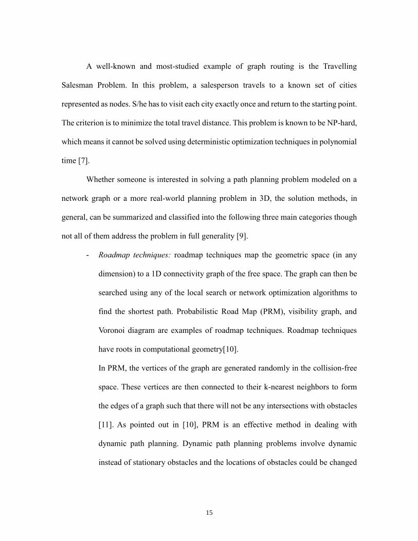
Whether someone is interested in solving a path planning problem modeled on a

network graph or a more real-world planning problem in 3D, the solution methods, in

general, can be summarized and classified into the following three main categories though

not all of them address the problem in full generality [9].

- Roadmap techniques: roadmap techniques map the geometric space (in any

dimension) to a 1D connectivity graph of the free space. The graph can then be

searched using any of the local search or network optimization algorithms to

find the shortest path. Probabilistic Road Map (PRM), visibility graph, and

Voronoi diagram are examples of roadmap techniques. Roadmap techniques

have roots in computational geometry[10].

In PRM, the vertices of the graph are generated randomly in the collision-free

space. These vertices are then connected to their k-nearest neighbors to form

the edges of a graph such that there will not be any intersections with obstacles

[11]. As pointed out in [10], PRM is an effective method in dealing with

dynamic path planning. Dynamic path planning problems involve dynamic

instead of stationary obstacles and the locations of obstacles could be changed

16

real-time, thus, they are not given a priori. However, Bhattacharya and

Gavrilova [10] claim that PRM could hardly meet the optimization criteria of

the path planning due to its probabilistic nature. Visibility and Voronoi (also

known as retraction) techniques are explained in detail in chapter 4.

- Motion planning: motion planning in robotics is a problem similar to routing or

path planning. The only difference is that in motion planning, the robot is not a

simple point and its configuration and topology should be taken into account

while planning for a collision-free path. However, since planning a path for an

agent with an arbitrary size and typically complex geometry is quite

challenging, robot motion planning introduces the concept of configuration

space. Configuration space is a way of representing the workspace by treating

the robot as a point, rather than an object with a complex geometry, traveling

from the initial point to a final point and modifying the geometry of the

obstacles instead to reflect the shape of the robot. Some of the common

techniques used widely in robot motion planning are potential fields and exact

or approximate cell decomposition.

In the Potential Field (PF) method, scalar functions similar to electrostatic

potentials are assigned to all nodes of the search graph. The potentials assigned

to the nodes lying on the obstacles are the highest. Knowing that the constraint

is to avoid any collisions, the objective is to find a path with the minimum

potential among all. The path can then be generated by following the steepest

descent directions of the potential toward the goal [12]. Despite its efficiency

17

in dealing with collisions in real time, the potential field has a major drawback.

As stated in [8], there usually could exist local minima at points other than the

goal point where the path could be stuck, which causes problems in reaching

the goal. The Cell decomposition technique is described in chapter 4.

- Mathematical programming: in contrast to the former techniques, mathematical

programming does not require a graph of the free space to identify the shortest

path. Unlike the other approaches, mathematical programming develops a

mathematical (optimization) model of the problem. Like any optimization

problem, one needs to define the optimization objective(s) and all applicable

constraints to be satisfied. The fundamental criterion of the shortest path

problem is obviously to minimize the length of the path while the constraint is

often times to avoid interference with obstacles. Solving this problem using

deterministic optimization techniques is almost impossible due to the

nonlinearity of the objective function (nonlinear Euclidean distances are to be

minimized as an objective) and difficulties in modeling the collision avoidance

constraints, mathematically. To overcome the problem of modeling the

constraints, researchers usually discretize the workspace as a grid and try to

drive the number of overlapping cells to zero. Overlapping cells are the cells of

the path interfering with the occupied cells in the obstacles. To avoid collisions,

the ratio of the overlapping cells over the total number of cells in the workspace

is calculated. This ratio is then entered into the objective function as a penalty

to be minimized [13]. Often, researchers use heuristics methods to solve this

18

optimization problem since heuristics can result in global optimal solutions.

However, heuristic methods result in different solutions each time they are run.

In addition to the modeling challenges, defining the design variables of the

optimization problem is not quite straightforward. In path planning problems,

design variables for the optimization problem are usually the x, y, and z

coordinates of the points located in the free space denoting the end points of a

line segment since the final path is a piecewise linear path consisting of several

line segments. Given this definition of the design variables, the number of

variables is not known a priori making the optimization modeling even more

difficult.

1.1 Objectives of this Research

The objectives of this research are to efficiently model the free space of the given

2D environment cluttered with arbitrary polygonal obstacles and then find the shortest

collision-free path connecting the initial and final points. The outcome of this research will

help to expand the solution idea to higher dimensions including 3D and to optimally route

cable harnesses in electro-mechanical systems.

The rest of this thesis is organized as follows. In the next chapter, a brief overview

of the literature on the path planning problem with the main focus on 2D path planning is

presented. In chapter 3, the geometric representation technique chosen in this research is

explained in detail. Chapter 4 is allocated to the general intersection detection techniques

for path planning problems and focuses on 2D detection techniques. Chapters 5 and 6 deal

with the construction of the free space graph and finding the shortest path through

19

searching that graph. In chapter 7 the results of the research followed by the validation and

case studies are presented. The main findings from implementing the developed algorithm

in this research are also summarized. The conclusions are drawn in chapter 8 and some

ideas for moving the research forward are provided as potential future work.

20

Chapter Two

LITERATURE REVIEW

The Path Planning problem has been widely studied in the literature. Path planning

in 2D environments typically involves simplifying the unoccupied space (free space) to a

graph of the free space. This graph is later explored using network optimization methods.

Extensive research has been done on the representation of this free space. Briefly, some of

the approaches to undertake the free space representation and generation include visibility

graphs, Voronoi diagrams, sweep volume, wavefront, and so on. In what follows, a brief

summary of the previous work done on this topic is provided.

2.1 State of the art in Roadmap techniques

One approach to model the free space is known as roadmap technique[9].

Roadmaps map the free space to a connectivity graph. Visibility graphs and Voronoi

diagrams are well-known examples of roadmaps and are explained in detail in chapter 5.

Constructing the visibility graph to model the free space is considered as the very

first method in computational geometry to address the shortest path problem in the

plane[14]. Visibility graph is an undirected graph of edges connecting every two nodes that

are visible to each other, meaning the edge they share does not intersect the interior of any

obstacle [14]. The algorithm is computationally expensive since it explores all the vertices

of all the obstacles. In fact, the fastest known algorithm to construct the visibility graph

developed by Asano et al. [15] has the time complexity of order O(n2) n being the total

number of obstacles’ vertices. Should one consider f objects with nave vertices on average

21

per object, then the complexity is of the order O(f2 nave 2) Therefore, research efforts have

been undertaken to improve the efficiency of the algorithm even further.

Focusing on improving the efficiency of visibility graphs, Rohnert [16] develops

an algorithm that computes the shortest path in a Euclidean plane in presence of a set of

disjoint convex polygonal obstacles in O (f2+nlogn) time, f being the number of the

obstacles and n the total number of vertices. To better understand the significance of this

improvement in the time complexity, one could take a numerical example. Suppose, there

exist 10 objects in the workspace with average 4 vertices per object, resulting in total 40

vertices in the plane. Asano’s algorithm implemented on this example yield a complexity

of (10*4)2 or 1600 while Rohnert’s algorithm results in a complexity of

O(102+40log40)=164 which is significantly lower.

Instead of generating the entire visibility graph of the workspace, to improve the

time complexity of the algorithm, Rohnert generates a part of the graph relevant in finding

the path between the start and termination points in O(n+f2logn) time. Based on a lemma

stated in this article, “the shortest collision free path from point s to t in the plane runs via

the edges of the polygonal obstacles and the supporting segments between the pairs of

polygons”[16]. Rohnert defines the supporting segment as a line segment of a common

tangent of the two polygons lying between the two points of contact of the tangent and the

polygon[16]. By this definition and based on the aforementioned lemma, the part of the

visibility graph needed to be constructed consists only of the edges of the polygons and the

supporting segments rather than all edges connecting the visible nodes. However, if the

supporting segment between a pair of polygons intersects the interior of another polygon,

22

the algorithm eliminates that segment from the graph while the segment could still be used

to generate the optimal solution. After the construction of the partial visibility graph,

Dijkstra’s algorithm is implemented to find the shortest path on the graph. Dijkstra’s

algorithm is explained in detail in chapter six. Rohnert uses the Dijkstra’s algorithm

developed by Tarjan and Fredman [17] that finds the shortest path in O(|E| +|V| log|V|)

time, |E| being the cardinality of the set of edges and |V| the cardinality of the set of vertices

in the graph.

Rohnert’s algorithm works efficiently for planes with convex polygonal obstacles.

However, it cannot deal with concave and more complex shapes. In addition, since it

eliminates the intersecting supporting segments and only keeps the “useful” ones besides

the polygon edges, hence restricting the feasible region, it may not be able to find the global

optimal solution.

In an independent study by Welzl [18], the construction of a visibility graph of a set

of L nonintersecting line segments is explained and the problem of finding the shortest path

between two points of the plane while avoiding intersection with these line segments is

addressed. The developed algorithm to construct the visibility graph has an improved time

complexity of order O(L2). The visibility graph is then searched using a standard single

source shortest path algorithm of Dijkstra.

Sharir and Schorr investigate the shortest paths in 2D and 3D spaces with

polyhedral obstacles [19]. For the 2D space, they develop an algorithm that constructs the

visibility graph of the environment with n total number of vertices in O(n2logn) time

although they present some special cases for which the time complexity of the construction

23

is of order O(nlogn). Taking the same numerical example, Sharir’s algorithm in general

case yield a complexity of (402*log40) =2563 which is the least efficient algorithm known

to construct the visibility graph.

The constructed visibility graph is then explored using Dijkstra’s algorithm

developed by Aho et.al. [20] in O(n2) time to find the shortest path. They also address the

more complicated 3D shortest path problem. They claim that the shortest path passes

through the points lying on the edges of the polyhedral obstacles. They develop a method

to find the sequence of those points through which the shortest path passes in doubly

exponential time (has the form ofxba ) which is much faster than factorial (O(n!)). Lastly,

they show a special case of the 3D shortest path problem along the surface of a convex

polyhedron which is solvable by their technique in O(n3logn).

Visibility graphs are not only constructed to act as the building blocks for the

optimization aspect of the path finding problems, but they are deployed in facility location

problems as well. Butt and Cavalier in their article [21], propose an algorithm to find an

optimal location to place a new facility X in presence of convex polygonal forbidden

regions the travel through which (and not along!) is prohibited such that the sum of the

distances from facility X to the existing facilities is minimized. They first generate the

visibility graph of the existing facilities and the polygonal forbidden regions. After

determining the visible nodes, the new facility, X, is introduced and the visible nodes of

the predetermined graph with respect to X are found. Then, the Euclidean distance of the

facility X to each of the existing facilities is defined and the location of the facility X is

determined such that the sum of the distances is minimized. In order to avoid searching the

24

entire environment for the location of X, based on a theorem that states the optimal location

of the new facility lies within the convex hull of the existing facilities[21], they only search

the region restricted by that convex hull. They also define N regions corresponding to the

N existing facilities to simplify the search for the location. With X lying inside each of the

different regions, the definition of the objective function will differ. The optimal location

of the facility X is the one that guarantees the minimum sum of the distances to the N

existing facilities.

In all the aforementioned research works, the planning occurs for an object reduced

to the size of a point. However, there are instances (especially in robotics) in which the

moving object itself is a polygonal or polyhedral object in 2D or 3D environments

respectively. In this case, an approach based on the Minkowski sum is utilized to take the

geometry of the moving object into account.

Lozano and Wesley [22] tackle the problem of planning a collision-free path for a

moving object of known geometry among polyhedral obstacles using visibility graphs.

They start with taking the 2D planning into account and move on to the 3D problem. Since

the moving object is no longer a point, construction of the visibility graph becomes a great

challenge. Hence, they first come up with a method to transform the object to a reference

point. To do so, they grow the obstacles by an offset related to the size of the moving object

and shrink the moving object to a reference point. The new obstacles represent the locus of

the positions of the reference point that cause a collision with the obstacles[22]. The

reference point can be any point of the moving object such as its center or corner points.

To find the configuration space of the problem, the authors take into account position as

25

well as the orientation of the object. After determining the configuration space, a visibility

graph need be constructed and finally searched for the shortest path.

One of the famous shortest path problems is the Traveling Salesman Problem as

briefly mentioned in the previous chapter. This NP-hard problem is of interest to a lot of

researchers working on the shortest path problems. Research is still going on to improve

the efficiency of the solution for the TSP problem.

Meeran and Shafie in [23] propose an algorithm to solve the TSP in polynomial

time using convex hulls generated by Graham’s method [14]. The idea behind their method

is based upon a proposition by Flood [24]which states that if all the cities in TSP lie on the

boundary of their convex hull, the TSP has an optimal solution. The initial sub-tour in this

algorithm is the boundary of the convex hull of the cities. They introduce a heuristic rule

to group cities into circular neighborhoods, the diameters of which are the edges of the sub-

tour convex hull. If a city has no neighborhood, children neighborhoods are created based

on the parent neighborhood until all cities are assigned to at least one neighborhood. If a

city belongs to more than one neighborhood, the neighborhood that yields the smallest

distance to that city is chosen as the main one. In this way, the algorithm inserts all cities

on the boundary of the convex hulls of the neighborhoods in order to achieve the optimal

path. The order of visiting the nodes is then optimized by the nearest neighbor [23] method.

The authors claim that by combining the solutions for the local search in each

neighborhood, the algorithm is able to yield the global solution.

The second most common roadmap method of constructing the graph of the

collision-free space is using the Voronoi diagram also known as retraction method [9].

26

Voronoi diagram of n vertices partitions a plane or space to n regions. An edge of a Voronoi

diagram is equidistant to two vertices. The technique of constructing the Voronoi diagram

is explained in chapter 5 in detail. Researchers have attempted to incorporate the Voronoi

diagrams in solving the path planning problem during the past decades especially for the

cases in which finding the maximum clearance path is the main criterion.

Bhattacharya and Gavrilova[25], tackle the problem of 2D path planning using

Voronoi diagrams and develop a shortest path algorithm that works in O(nlogn) time, n

being the total number of vertices. They start with creating the Voronoi diagram of the

workspace by approximating the obstacles by their boundary points, and dynamically add

the start and target points into the diagram. Then, they connect the start and target points

to all Voronoi vertices to avoid intersections. Next, they define the minimum clearance (c)

from the obstacles and remove all the edges of the Voronoi diagram that result in a

clearance less than c. Now the graph is ready to be searched for the shortest path. The

search algorithm of their choice is Dijkstra’s [26]. However, the solution found might

require some smoothing and refinement since the shortest path includes redundant vertices

and unnecessary turns.

To achieve both the shortest path and the maximum clearance from the obstacles,

researchers use Voronoi diagrams in conjunction with visibility graphs to take advantage

of both yielding the shortest path and ensuring a certain amount of clearance from the

obstacles.

Wein et.al present an algorithm in their paper [27]to find the shortest path that is

both smooth and guarantees a clearance c from the obstacles. They improve the efficiency

27

of their algorithm to a time complexity of O(n2logn) for total n vertices, over the time-

expensive visibility graph construction. The algorithm evolves from a visibility graph to a

Voronoi diagram as c grows from 0 to ∞. In the preprocessing phase, they dilate the

polygonal obstacles by c using the Minkowski sum of the polygon and a disk of radius c.

They then, construct the visibility graph of the dilated obstacles and in case a narrow

passage is blocked by two or more dilated obstacles, they find the intersection of the union

of dilated obstacles and the Voronoi diagram, hence replacing the blocked portion by a

Voronoi edge passing through the narrow passage. Although the clearance of the Voronoi

edge from the blocking obstacles is less than c and it may yield sharp turns, to ensure that

the path is optimal in terms of its length, this passage is allowed by this algorithm. The

graph is later searched by Dijkstra’s algorithm to find the shortest path. Despite the proved

efficiency of this algorithm, it may not be practical to implement this algorithm on a large

scale problem as mentioned in [25].

In another paper by Clarkson [28], a method is proposed to improve the time

complexity of the visibility-based shortest path algorithm. The developed speed-up

technique works on eliminating some of the unnecessary edges of the visibility graph

through generating the Minimum Spanning Tree (MST) of the vertices of the obstacles.

The MST of a set of nodes is the minimum length tree that spans all the nodes [14]. The

new graph (sub-graph) is a subset of the original visibility graph that need be augmented

by the start and end points of the path. To find this augmented subgraph, Clarkson uses the

conical Voronoi diagrams of the vertices in his algorithm. He then deploys the algorithm

developed by Fredman and Tarjan [17] to find the ε-shortest path. The ε-short path is the

28

path that has a length no longer than (1+ε) times the shortest path between s and t .

Clarkson’s algorithm is capable of constructing the data structure in O(nlogn) and finding

the ε-short path in 2D cases in O(nlogn+n/ε) time, with n being the total number of vertices

and ε a given value satisfying 0 ≤ 𝜀 ≤. The algorithm works both on 2D as well as 3D

spaces with slight changes in the vertices of the visibility graph of the 3D space.

Roadmap techniques are not limited to the visibility and Voronoi methods. For

example, Hershberger and Suri[29] propose a method to solve the shortest path problem in

a plane with significant improvement in the time complexity over the previously developed

techniques. The proposed technique is capable of finding the optimal solution to the

shortest path problem in O(nlogn) time using wavefront propagation technique. Wavefront

propagation roughly imitates Dijkstra’s algorithm by simulating the propagation of a wave

from a source node to other nodes of the shortest path map spreading among the obstacles.

The wavefront at time t includes all points of the plane with distance t from the source

node[29]. This algorithm has been proved to find the shortest path in O(n2) time previously,

however, the authors of this article propose two speed-up techniques that improve the time

complexity of the wavefront propagation up to O(nlogn). The first speed-up

implementation corresponds to a quad-tree style subdivision (conforming subdivision) of

the plane and the second one approximates the wavefront. Conforming subdivision splits

the plane into a linear number of cells using vertical and horizontal edges generating the

shortest path map for the wavefront to travel through. By subdivision of the plane, the

propagation of the wavefront is guided through the subdivided cells, resulting in expediting

the process of finding the shortest path. In each cell, a Voronoi diagram technique is

29

deployed to take care of the collisions and provide the edges of the shortest path map.

Vertices of the map are the vertices of the obstacles.

2.2 3D shortest path problem

In addition to the mathematical modeling and graph construction methods, scholars

have also studied more applied path planning problems such as pipe routing in ships and

chemical process plants, wire and/or cable routing in automobiles and aircrafts, robot

motion planning and so forth. In what follows, a brief overview of the state of the art in the

applied path planning problems is provided. These problems are mainly in 3D spaces.

Yin et al. [30], solve the 3D pipe routing problem representing the physical

obstacles by their vertices and convex hulls in 3D space. They claim that the shortest path

for a pipe while avoiding convex obstacles is the path through an obstacle’s edges. Then,

they use the visibility graph approach to find the candidate edges and nodes of the shortest

path.

Cagan and Szykman [31] propose an approach based on Simulated Annealing (SA)

to produce non-orthogonal routes for pipes in a 3D environment. Given the locations for a

pair of terminals, an initial route, which is the straight line between the two terminals, is

chosen. Then, the optimizer based on SA moves the locations of bend points, which are

design variables to minimize an objective which consists of the sum of three components:

the total length of the route, the number of bends, and the degree of penetration inside

obstacles. Weights are used to distribute the importance of the three objectives, and the

aim is to drive the third one (obstacles interference) to 0. In [13], Sandurkar and Chen

solve a pipe routing problem in 3D space using the tessellated format (triangles and nodes)

30

to represent components in the workspace as obstacles, which enables them to handle both

convex and concave objects along with a Genetic Algorithms (GA) that determines angles

and lengths of each segment of a single pipe. To detect interference with obstacles, they

use an interference checking program, RAPID, developed at the University of North

Carolina [32].

Conru and Cutkosky [33] address the cable harness problem by starting with the

generation of an initial solution without considering any obstacles. Then, the obstacles are

introduced gradually and the path is refined to satisfy collision avoidance constraints. In a

Separate study [34], Conru uses a GA technique to find near-optimal solutions for cable

harness routing in a 3D environment consisting of nodes. He starts with a random

configuration of cable harness and refines it using a GA.

The automotive wire routing and sizing for weight minimization is addressed in

[35] using the minimal Steiner tree algorithm and Linear Programming (LP) formulation

on a predefined graph. Also, authors of [36] address the problems of wire routing, wire

sizing, and consider the allocation of splices in their paper. They use a depth-first (graph

traversing) approach to compute the minimal cost path and a two-phase heuristic with a

Simulated Annealing (SA) algorithm to tackle the wire sizing problem.

Researchers have also looked into cable harness routing problem. Zhu et al. [37]

propose a bi-level optimization approach to find optimal paths for wire harnesses in an

aircraft. They assert that since cable harness routing is a multi-destination path finding

problem, simple routing algorithms to find shortest paths between two points do not result

in accurate optimal solutions. They perform a two-step hybrid strategy to tackle this

31

problem. The first step, initialization, generates a preliminary harness configuration using

a roadmap technique. The second step deals with the optimization part to refine the

preliminary configuration. In the local level of their bi-level optimization method, they use

the A* search algorithm to find optimal paths between two end points of a branch. And, in

the harness level, which they call global optimization level, they use a Hill Climbing

algorithm to come up with an optimal solution for the whole harness. The objective

function of this problem is the harness cost which itself is a function of three variables:

length of the harness (as summation of the lengths of all bundles in the harness), number

of clamps to fix harness on the airframe, and the amount of protecting layers to protect the

harness from harsh areas (humid, hot, and vibratory areas). The design variables are the

coordination of the clamps and transition points. Also, there are three constraints that need

to be satisfied while designing the wire harnesses: minimum bend radius, maximum

clamping distance (distance between two adjacent clamps), and minimum fixing distance

(distance from the center of harness curve and its fixing structure).

As could be implied from the above listed research articles, to solve the 3D path

planning problems, researchers mainly use heuristic techniques. These techniques though

capable of yielding the global optimal solution, are approximations and have greater time

complexities than exact methods since they search the entire feasible region for an optimal

solution.

Although many research works have tackled the path-planning problem and

improved the efficiency of the current geometric approaches, some limitations still exist in

this field. Chen in his short article [38], after defining the geometric shortest path problem

32

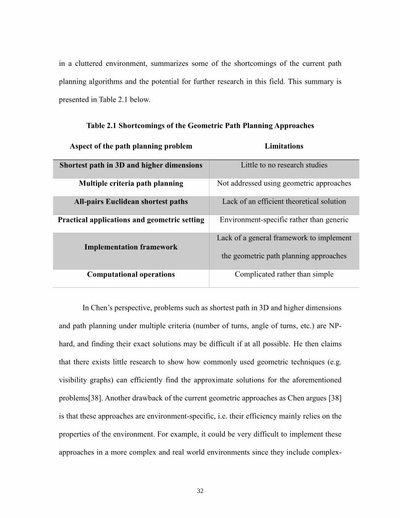
in a cluttered environment, summarizes some of the shortcomings of the current path

planning algorithms and the potential for further research in this field. This summary is

presented in Table 2.1 below.

Table 2.1 Shortcomings of the Geometric Path Planning Approaches

Aspect of the path planning problem Limitations

Shortest path in 3D and higher dimensions Little to no research studies

Multiple criteria path planning Not addressed using geometric approaches

All-pairs Euclidean shortest paths Lack of an efficient theoretical solution

Practical applications and geometric setting Environment-specific rather than generic

Implementation framework

Lack of a general framework to implement

the geometric path planning approaches

Computational operations Complicated rather than simple

In Chen’s perspective, problems such as shortest path in 3D and higher dimensions

and path planning under multiple criteria (number of turns, angle of turns, etc.) are NP-

hard, and finding their exact solutions may be difficult if at all possible. He then claims

that there exists little research to show how commonly used geometric techniques (e.g.

visibility graphs) can efficiently find the approximate solutions for the aforementioned

problems[38]. Another drawback of the current geometric approaches as Chen argues [38]

is that these approaches are environment-specific, i.e. their efficiency mainly relies on the

properties of the environment. For example, it could be very difficult to implement these

approaches in a more complex and real world environments since they include complex-

33

shaped obstacles or obstacles whose shapes/geometry do not remain fixed. He also believes

that there still does not exist a general framework to implement these geometric approaches

and the user needs to develop the code on his or her own. Hence, the practitioner must first

study a great deal of geometric techniques and data structures to be able to program a path

planning method. On the other hand, often times the geometric approaches involve too

many computational operations and sophisticated geometric procedures (such as visibility

graphs, Voronoi diagrams, triangulations, etc.) and/or data structures. Lastly, as a

suggestion, Chen proposes that the researchers look into developing more general (rather

than problem-specific) yet simple-to-implement geometric algorithms to fulfill the

necessity of solving a path planning problem in a more general and even complex

geometric setting. From his point of view, the efficiency of this general approach will

depend more on the configuration of the input rather than its size.

In addition to Chen’s summary of shortcomings, there are limitations corresponding

to the current roadmap techniques of solving the shortest path problem. For example,

Voronoi diagram despite being efficient in dealing with the collision avoidance aspect of

the path planning, yields sub optimal solutions since the path would be longer and with

more turns than needed. Also, visibility graph is not computationally efficient since

explores all nodes of the environment while in some path planning problems only a portion

of the workspace may be involved, hence no need to explore all the vertices of the obstacles

by the expense of increasing the computation time.

34

2.3 Research Questions

Based on the study of the literature and previous research, we propose a new

method to tackle the planar path planning in a cluttered environment that has a potential to

be implemented in 3D environments as well.

The main research question to be addressed is whether or not there is an efficient

way with less time complexity than the visibility graph to preprocess the path planning

problem and construct the graph of the free space. The objective is to find multiple collision

free paths (if there exists any) forming the graph of the free space in presence of various-

shaped stationary and disjoint obstacles in a 2D workspace regardless of the size of the

workspace. The next question to be addressed is if it is possible to find the shortest path on

the found free space graph using any network optimization algorithm.

35

Chapter Three

GEOMETRIC REPRESENTATION

Geometric representation of the workspace and the associated data is paramount in

planning a collision-free path in a cluttered environment. Since the intersection detection

and optimization domains in the path-finding algorithms rely on the geometric data, the

entire workspace needs to be well represented.

In the following sections, the types of geometric representations, the advantages of

using tessellated formats and the data structures used to represent and manipulate the

geometric data in this research are discussed.

3.1 Geometric Representation Schemes

There are various types of geometric representation schemes to create solid models

in CAD software packages. However, the two most popular schemes are Constructive Solid

Geometry (CSG) and Boundary Representation (B-rep) [39].

The general idea behind the CSG model is that a physical object can be decomposed

into a set of primitives. Primitives act as building blocks of a solid model. They are basic

shapes that can generate solid models of any physical object using mathematical Boolean

operations [39]. The most widely used examples of primitives are rectangular block,

cylinder, cone, plane, and sphere.

On the other hand, a B-rep model is built upon the notion that a physical object is

surrounded by a finite number of faces. These faces are closed (a continuous region in

space without breaks) and orientable (the two sides of the face are distinguishable through

36

the direction of the surface normal). A B-rep model consists of faces, edges, and vertices

connected together to shape the object.

By this definition, the representation used in this research fall into B-rep models

since we are mainly dealing with the vertices and edges of the objects in the workspace as

explained in the upcoming chapters, though a CSG could also generate the model of such

a 2D workspace.

For the purpose of this research, the objects of the workspace are first modeled in

a CAD software, SolidWorks, with a B-rep scheme. For the 2D workspace, the objects are

created as 2D planar surfaces as shown in Figure 3.1. The tessellated format of the solid

model along with the VRML file format are used to easily exchange the file between

different CAD packages and between CAD packages and other data manipulation software.

Tessellated file formats are explained in the next section.

Figure 3.1: Sample Solid Model of a Workspace

37

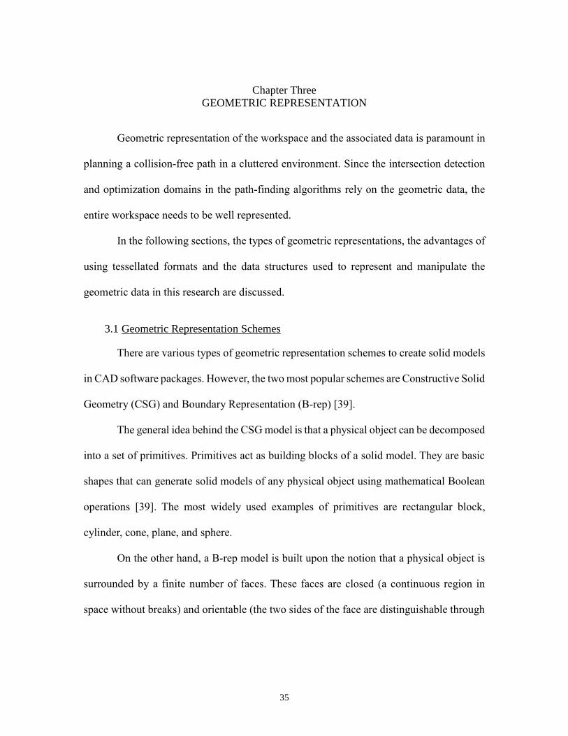
3.2 Tessellated Representation

In this research, the tessellated format of all the objects involved in the workspace

is used. The 2D planar solid models of the components are created using the

STereoLithography (STL) format in SolidWorks®. STL is a standard file format that

facilitates data exchange between CAD software and other systems, primarily 3D printers.

STL files are developed based on the triangulations of the solid models in order to facilitate

the handling of any free-form shapes for the solid model. In addition, the data needs to be

extracted from a CAD software to be able to be manipulated in the packaging and routing

problem. Since a case study of routing in 3D will be to route cables and harnesses of a

vehicle under-hood (previously addressed for the packaging optimization problem) in

which the components are tessellated. Hence, to generalize the algorithm we need to use

the tessellated format of the objects for consistency. Figure 3.2 below shows the tessellated

components of the vehicle under-hood.

Figure 3.2: Tessellated Under-hood Components

38

An STL file of a solid model includes the X, Y, and Z coordinates of each triangle’s

vertices as well as the coordinates of the normal to the surface of that triangle. An edge

must be shared by no more than two triangles. STL data can come in two representations:

ASCII or binary. Both representations contain same geometric information in accordance

with the STL file, though binary format requires less amount of memory to store the data.

Nevertheless, ASCII can be read easily since it provides a better visualization of data [40].

Figure 3.3: Sample STL File of a Workspace in ASCII Format

As can be seen from Figure 3.3, the ASCII file does include coordinates of triangles,

34 in total, and surface normals. However, it is not quite clear which triangle belongs to

which object in Figure 3.1. The ASCII STL file of the represented workspace occupies 10

KB of the memory, approximately.

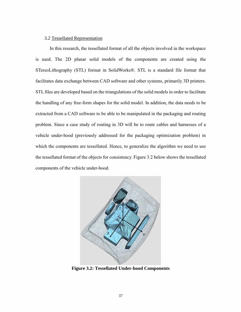
Despite the efficiency of the STL format and its strengths in tessellating solid

models, it has some accuracy issues as described in[40]. First, it may be possible that one

edge is shared by more than two triangles. This needs to be corrected, since, as mentioned

39

before, each edge should be shared by no more than two triangles. This erroneous situation

is shown in Figure 3.4.

Figure 3.4: Shared edge of a triangulated solid

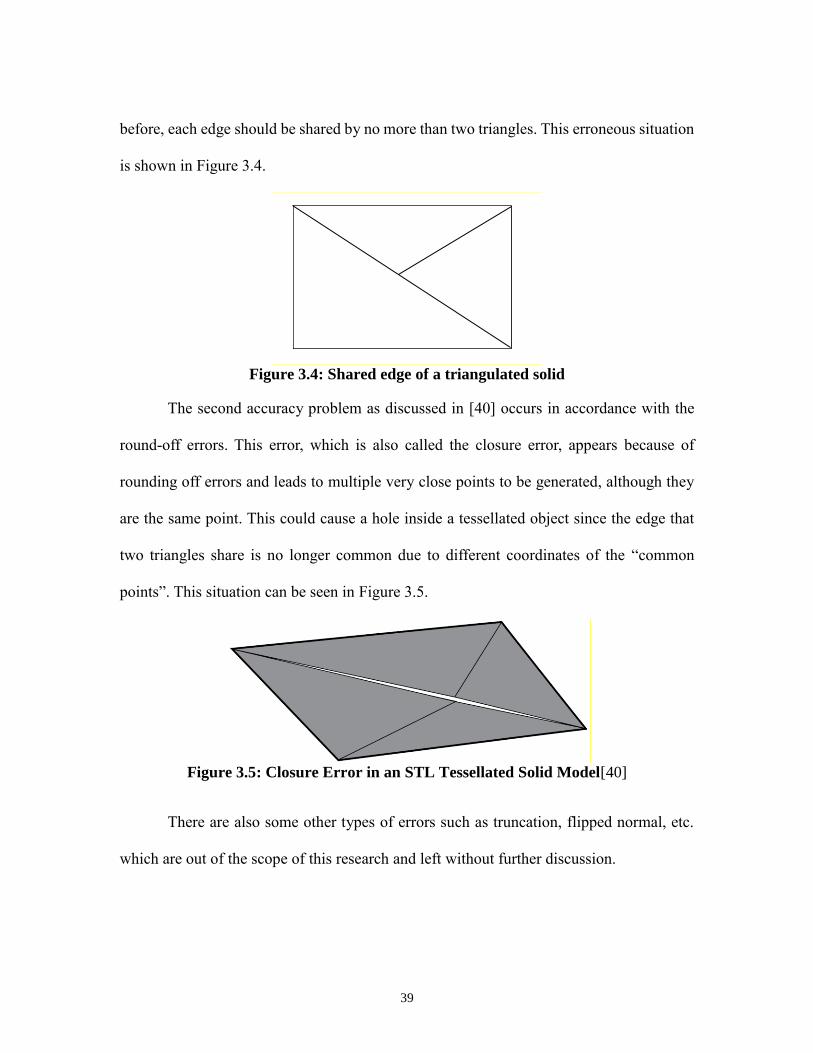
The second accuracy problem as discussed in [40] occurs in accordance with the

round-off errors. This error, which is also called the closure error, appears because of

rounding off errors and leads to multiple very close points to be generated, although they

are the same point. This could cause a hole inside a tessellated object since the edge that

two triangles share is no longer common due to different coordinates of the “common

points”. This situation can be seen in Figure 3.5.

Figure 3.5: Closure Error in an STL Tessellated Solid Model[40]

There are also some other types of errors such as truncation, flipped normal, etc.

which are out of the scope of this research and left without further discussion.

40

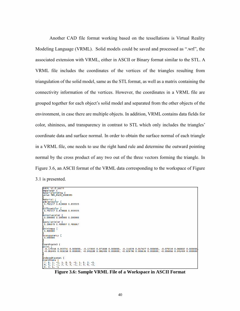
Another CAD file format working based on the tessellations is Virtual Reality

Modeling Language (VRML). Solid models could be saved and processed as “.wrl”, the

associated extension with VRML, either in ASCII or Binary format similar to the STL. A

VRML file includes the coordinates of the vertices of the triangles resulting from

triangulation of the solid model, same as the STL format, as well as a matrix containing the

connectivity information of the vertices. However, the coordinates in a VRML file are

grouped together for each object’s solid model and separated from the other objects of the

environment, in case there are multiple objects. In addition, VRML contains data fields for

color, shininess, and transparency in contrast to STL which only includes the triangles’

coordinate data and surface normal. In order to obtain the surface normal of each triangle

in a VRML file, one needs to use the right hand rule and determine the outward pointing

normal by the cross product of any two out of the three vectors forming the triangle. In

Figure 3.6, an ASCII format of the VRML data corresponding to the workspace of Figure

3.1 is presented.

Figure 3.6: Sample VRML File of a Workspace in ASCII Format

41

Figure 3.6 includes the coordinate data for one of the objects in the workspace

shown in Figure 3.1.

Both VRML and STL could generate ASCII as well as Binary formats of the

geometric data associated with the solid model. However, the ASCII format is more

human-readable and the flow of information can be more easily understood. Hence, we use

the ASCII format in all the CAD data analysis of this research.

A comparison of Figure 3.3 and Figure 3.6 shows that the VRML file is more

organized in terms of the data for each object. It explicitly shows which vertices of an

object are connected to each other and the coordinates of the vertices are not repeated for

each relevant triangle. Furthermore, VRML is efficient and more practical in data exchange

over the web [41] which makes it a better option for collaborative design projects. Besides,

VRML format occupies less storage. For example, the VRML format of the workspace of

Figure 3.1 only takes 6KB whereas its STL counterpart takes approximately 10KB. Hence,

as the scale of the problem becomes larger there will be more difficulties in storing data as

STL. Above all, the VRML format does not result in the closure or other types of errors

challenge the STL format. Considering the advantages of VRML over STL, all CAD data

in this research is saved and processed as .wrl files.

After creating the solid model of the workspace and generating the corresponding

geometric data, the VRML data needs to be imported to the main program for

manipulations. We use MATLAB to program the algorithm and find the safe path since it

could deal with matrices and vectors efficiently.

42

The geometric data in .wrl format is thus imported into the MATLAB code and all

the vertices and faces are read using a function listed in Appendix A. After the data is read,

a matrix that includes the number of elements of the workspace, the coordinates of the

vertices and the connecting edges is generated. This matrix is further used for the

intersection check, graph generation, and pathfinding processes that are explained in the

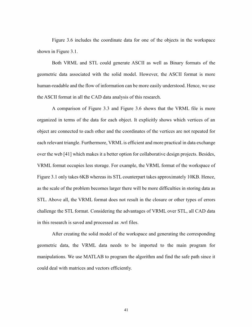
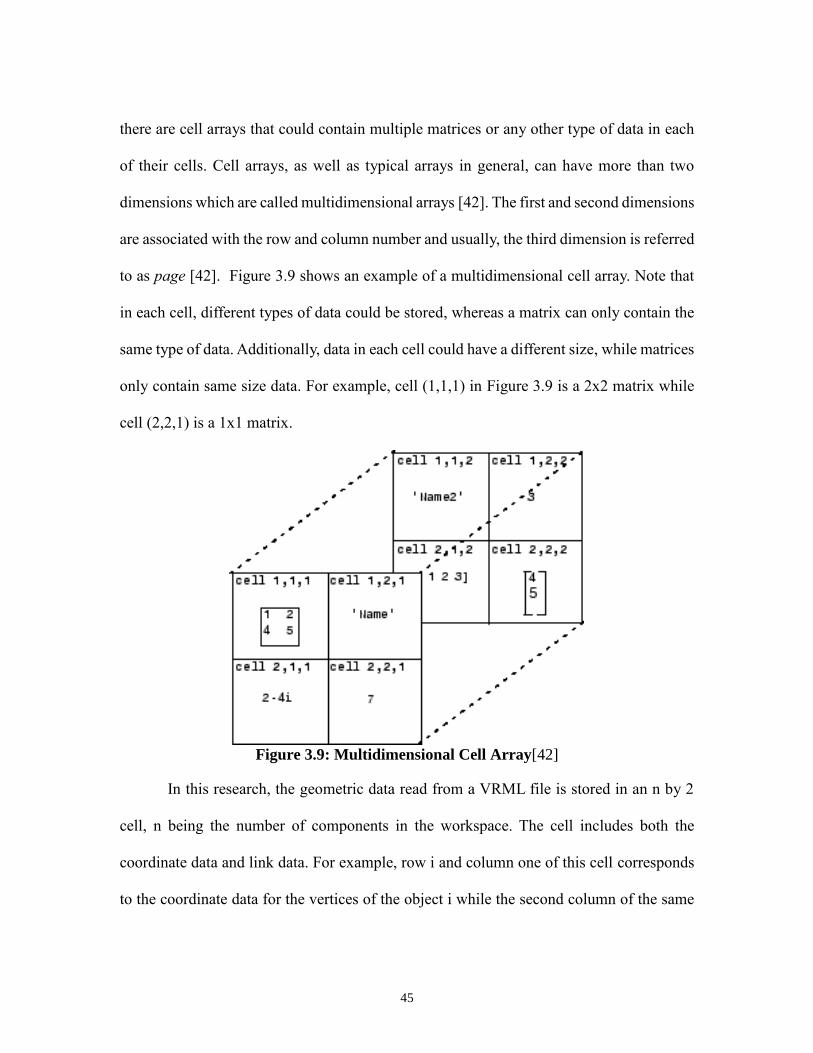
upcoming chapters. The tessellated workspace of Figure 3.1 is plotted using the

aforementioned matrix of geometric data imported in MATLAB and depicted in Figure 3.7.

Figure 3.7: Sample Tessellated 2D Workspace Imported in MATLAB

This figure shows eight planar objects scattered in the workspace. The objects have

convex as well as non-convex shapes that could be easily handled with tessellations. The

triangles in each object represent the tessellations performed on the solid model. In

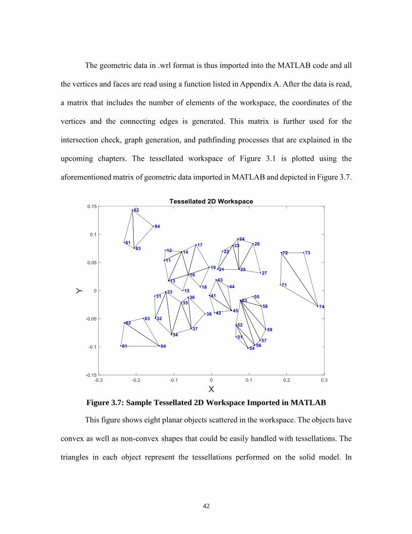
43

addition, each vertex is numbered. These numbers are unique IDs assigned to each vertex

to identify them. If there are no more than 10 objects in the workspace, the first digit of

each node ID shows the corresponding object to which the vertex belongs. The rest of the

digits show the vertex index in that object, which is generated by the VRML file

automatically. For example, node 54 in Figure 3.7 corresponds to vertex number 4 of object

5. However, this numbering does not work in the case where there are more than 10 objects.

For example, suppose the ID of a node is 2045. This ID could be interpreted both as node

45 of object 20 and node 5 of object 204. Hence, to distinguish between these IDs, a new

node numbering system is proposed for the workspaces containing more than 10 objects.

In this case, the object number is multiplied by 1000 (or any big number) and the node

number is added to it. By this numbering system, node 45 of object 20 has ID of 20045

while node 5 of object 204 has the ID of 204005, which are unique.

Figure 3.8: Planar Workspace after the Elimination of the Interior Edges

44

For the planar (2D) path planning, there is no need to include the interior edges

caused by the tessellation of the workspace since the path is not allowed to pass through

those edges. Hence, the interior edges of the tessellated surfaces are excluded in this

research. However, for the 3D path planning, there is no restriction on passing through the

interior edges of the outer surfaces of an obstacle as long as it does not intersect the interior

of the obstacle. A sample resulting workspace after the elimination of the interior edges is

shown in Figure 3.8. One should note that keeping the interior edges does not interfere with

the process of finding the shortest path following the proposed algorithm in this research

except that it occupies memory and may slow down the computations slightly.

The next section of this chapter is allocated to the data structures used in the

MATLAB program for this research.

3.3 Data Structures

Data structures are important when it comes to storing, organizing, and processing

data. Choosing the correct data structure leads to less memory storage and shorter run-

times of a code.

Since the coordinates of the vertices are real numbers, the primary data type would

be in the form of double, which could deal with larger floating points. The composite data

structures for storing and implementation used in this research are as the follows:

- Array:

Arrays are one of the basic data structures in every programming language. An

array could store vector data of any primitive structures. Matrices could be created by

combining multiple arrays. In fact, arrays are one-dimensional matrices. On the other hand,

45

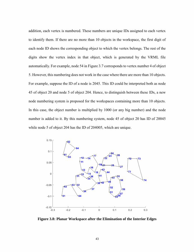
there are cell arrays that could contain multiple matrices or any other type of data in each

of their cells. Cell arrays, as well as typical arrays in general, can have more than two

dimensions which are called multidimensional arrays [42]. The first and second dimensions

are associated with the row and column number and usually, the third dimension is referred

to as page [42]. Figure 3.9 shows an example of a multidimensional cell array. Note that

in each cell, different types of data could be stored, whereas a matrix can only contain the

same type of data. Additionally, data in each cell could have a different size, while matrices

only contain same size data. For example, cell (1,1,1) in Figure 3.9 is a 2x2 matrix while

cell (2,2,1) is a 1x1 matrix.

Figure 3.9: Multidimensional Cell Array[42]

In this research, the geometric data read from a VRML file is stored in an n by 2

cell, n being the number of components in the workspace. The cell includes both the

coordinate data and link data. For example, row i and column one of this cell corresponds

to the coordinate data for the vertices of the object i while the second column of the same

46

row includes the connectivity data indicating the links which connect pairs of vertices of

object i.

Another important type of arrays which is used extensively in this research is the

dynamic array. A dynamic array is a variable-size array used whenever predefining an array

is not possible or the array size is not known a priori. For example, in creating a path

consisting of multiple connected points and line segments, the number of points may not

be known in the beginning assuming that a path is created by putting the points alongside

each other. In this case, defining the path as a dynamic array would be helpful in creating

the path by adding a point at each iteration until reaching the goal point.

- Record or struct

A struct is a set of fields similar to cell except a struct could contain both numeric

and character or string type data while cell could only store data of the same type.

- Graph

This data structure is critical in any routing problem. Since 2D problems mainly

work with graphs and there typically exists a graphical model of the workspace which is

searched for the safe shortest path, the graph data structure needs to be defined and created

correctly. This graph includes the start and end node and the connectivity nodes and edges

between them.

The data structure used in different parts of this research is explained in more detail

as different parts of the algorithm are discussed.

After representing the workspace geometrically and building the foundation of the

pathfinding method, the intersection detection and development of the free-space graph

47

used for calculating the shortest path is built upon this foundation and further discussed in

the upcoming chapters.

48

Chapter Four

INTERSECTION DETECTION

Generic path planning problems involve a planar (2D) or spatial (3D) workspace

occupied by certain (or even uncertain) number of objects. Such problems cannot be treated

as network or graph optimization problems since there does not exist a predefined graph or

network of nodes to search for the shortest path between a pair of nodes, instead, a

workspace containing multiple objects is given. Hence, care must be taken while planning

a path to ensure its safety. Safety of the path is defined by a metric related to the avoidance

of intersections with the interior of the objects called obstacles. Before avoiding such

probable collisions, one has to detect the possibility of the intersection. In this chapter, the

intersection detection technique utilized in this research is explained in detail.

As the shortest path between any two points is simply the straight line connecting

them, we need to check if that line intersects with the interior of any of the obstacles. If

there is no intersection, the straight line is the shortest path. Otherwise, the path must be

re-routed until a new collision-free shortest path is identified.

4.1 State-of-the-art in Interference Detection

Interference detection is a common problem in any path or motion planning

problem and it could be seen as the bottleneck of the path-planning problem. Once one

guarantees the path is collision-free, the shortest path could be found using any

optimization algorithm developed for this purpose.

Interference detection or collision avoidance occurs inevitably in robot motion

planning problems. Robotics researchers, mostly model the collision avoidance constraints

49

as forbidden regions of the workspace [22]. In other words, they take the components of a

2D or 3D workspace and model the obstacles as areas of 2D or volumes of the 3D

workspace where the path is not allowed to go through.

Sandurkar and Chen[13] solve a pipe routing problem in 3D space using Genetic

Algorithms (GA) that determines angles and lengths of each segment of a single pipe. To

detect interference with obstacles in the environment, they use an interference-checking

library, RAPID, developed at the University of North Carolina [32]. This library is capable

of detecting collisions in large environments containing unstructured objects.

4.2 Bi-level Collision Detector

In this research, we develop a bi-level collision detection algorithm that checks for

intersections between a line specified by the start and end points of the path and the objects

of the 2D workspace modeled as polygons.

The first level or the boundary check level of this algorithm checks if a polygonal

obstacle is within the boundary limits of the line connecting the start and end points of the

path and filters the out-of-bound obstacles out. The obstacles could have any convex or

nonconvex shapes since the workspace representation is based on the tessellations which

are capable of handling any free-form solid model through triangulations.

The first step in the boundary check is to rotate the coordinate system of the

workspace about Z axis and with respect to the line such that the new X-axis lies on the

start-end line and translate the origin onto the start point of the line. Later on, it is shown

how this coordinate transformation helps to simplify the computations for intersection

detection. By rotating the coordinate system about the Z-axis (out of the x-y plane of the

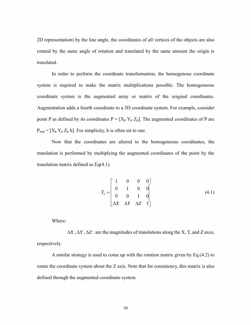
50

2D representation) by the line angle, the coordinates of all vertices of the objects are also

rotated by the same angle of rotation and translated by the same amount the origin is

translated.

In order to perform the coordinate transformation, the homogenous coordinate

system is required to make the matrix multiplications possible. The homogeneous

coordinate system is the augmented array or matrix of the original coordinates.

Augmentation adds a fourth coordinate to a 3D coordinate system. For example, consider

point P as defined by its coordinates P = [Xp Yp Zp]. The augmented coordinates of P are

Paug = [Xp Yp Zp h]. For simplicity, h is often set to one.

Now that the coordinates are altered to the homogeneous coordinates, the

translation is performed by multiplying the augmented coordinates of the point by the

translation matrix defined as Eq(4.1).

1 0 0 0

0 1 0 0

0 0 1 0

1

TT

X Y Z

(4.1)

Where:

X , Y , Z : are the magnitudes of translations along the X, Y, and Z axes,

respectively.

A similar strategy is used to come up with the rotation matrix given by Eq.(4.2) to

rotate the coordinate system about the Z axis. Note that for consistency, this matrix is also

defined through the augmented coordinate system.

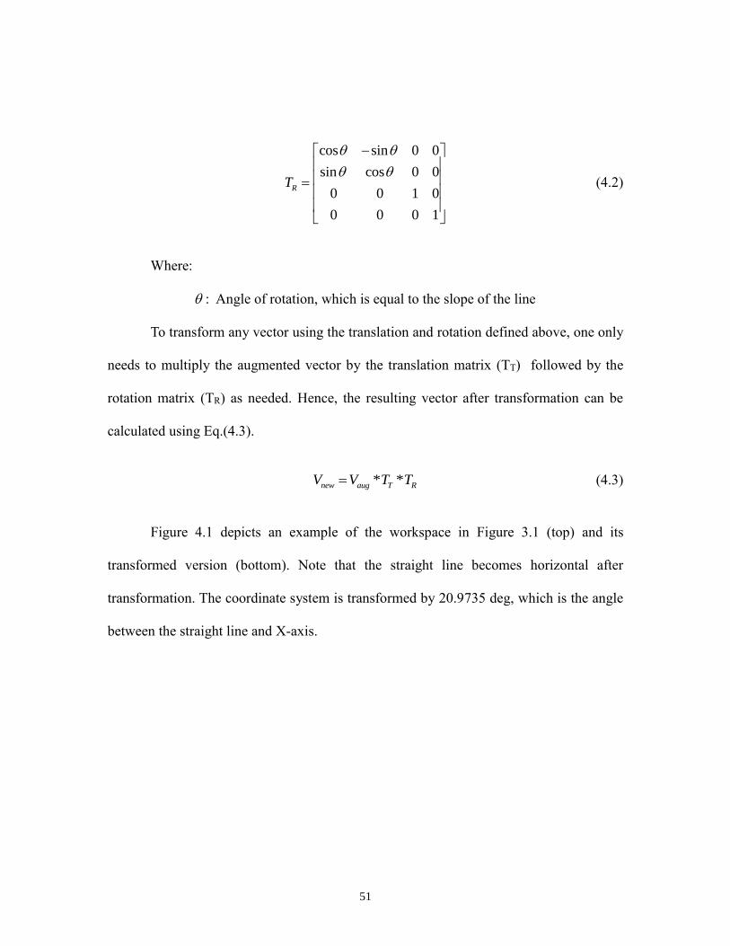
51

cos sin 0 0

sin cos 0 0

0 0 1 0

0 0 0 1

RT

(4.2)

Where:

: Angle of rotation, which is equal to the slope of the line

To transform any vector using the translation and rotation defined above, one only

needs to multiply the augmented vector by the translation matrix (TT) followed by the

rotation matrix (TR) as needed. Hence, the resulting vector after transformation can be

calculated using Eq.(4.3).

* *new aug T RV V T T (4.3)

Figure 4.1 depicts an example of the workspace in Figure 3.1 (top) and its

transformed version (bottom). Note that the straight line becomes horizontal after

transformation. The coordinate system is transformed by 20.9735 deg, which is the angle

between the straight line and X-axis.

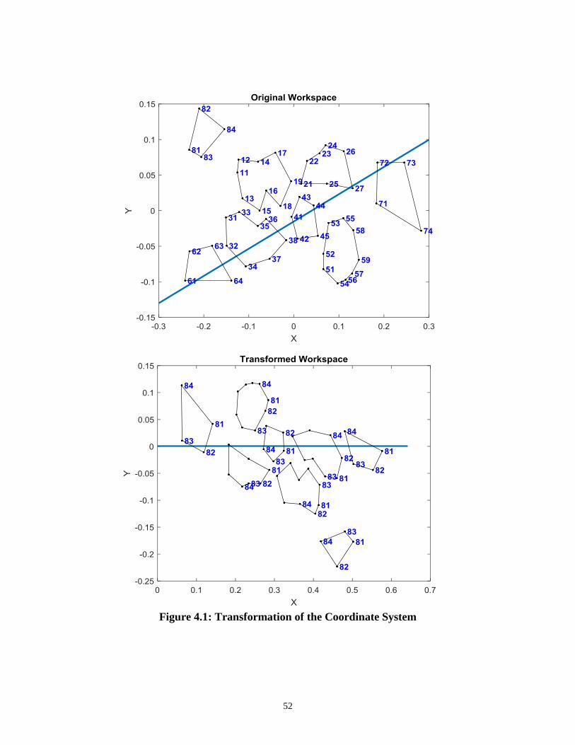
52

Figure 4.1: Transformation of the Coordinate System

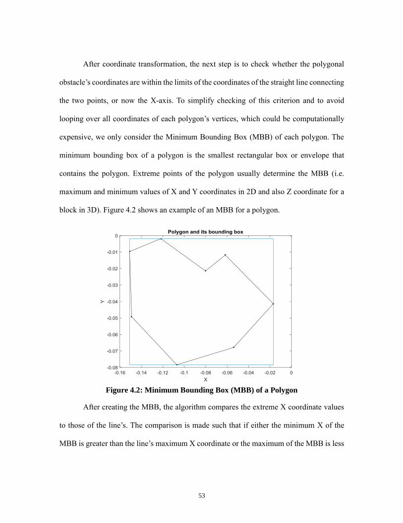
53

After coordinate transformation, the next step is to check whether the polygonal

obstacle’s coordinates are within the limits of the coordinates of the straight line connecting

the two points, or now the X-axis. To simplify checking of this criterion and to avoid

looping over all coordinates of each polygon’s vertices, which could be computationally

expensive, we only consider the Minimum Bounding Box (MBB) of each polygon. The

minimum bounding box of a polygon is the smallest rectangular box or envelope that

contains the polygon. Extreme points of the polygon usually determine the MBB (i.e.

maximum and minimum values of X and Y coordinates in 2D and also Z coordinate for a

block in 3D). Figure 4.2 shows an example of an MBB for a polygon.

Figure 4.2: Minimum Bounding Box (MBB) of a Polygon

After creating the MBB, the algorithm compares the extreme X coordinate values

to those of the line’s. The comparison is made such that if either the minimum X of the

MBB is greater than the line’s maximum X coordinate or the maximum of the MBB is less

54

than the line’s minimum X coordinate then the polygon is out of the line’s range and there

is no probability of having interference.

If the X coordinates of the polygon’s MBB are within the range of X coordinates

of the line, there could be a possibility of collision. Hence, further investigation is needed

to determine the intersection. If the polygon, whose MBB is in the range of the line’s

minimum and maximum coordinates, lies on either side of the line within the line’s X

values, there will not be any chance of having a collision. This condition is demonstrated

in Figure 4.3.

Figure 4.3: Example of a Polygon Lying at One Side of the Line

Therefore, checking if the polygon is within the X coordinate range of the line is

not sufficient to ensure the possibility of collision. To check whether the polygon intersects

the line or not, we need to also check the Y coordinates of the MBB. Since after rotation,

the X-axis of the coordinate system lies on the line, any point on the line must have zero Y

coordinate, and any point not lying on the line either has a negative or positive Y coordinate

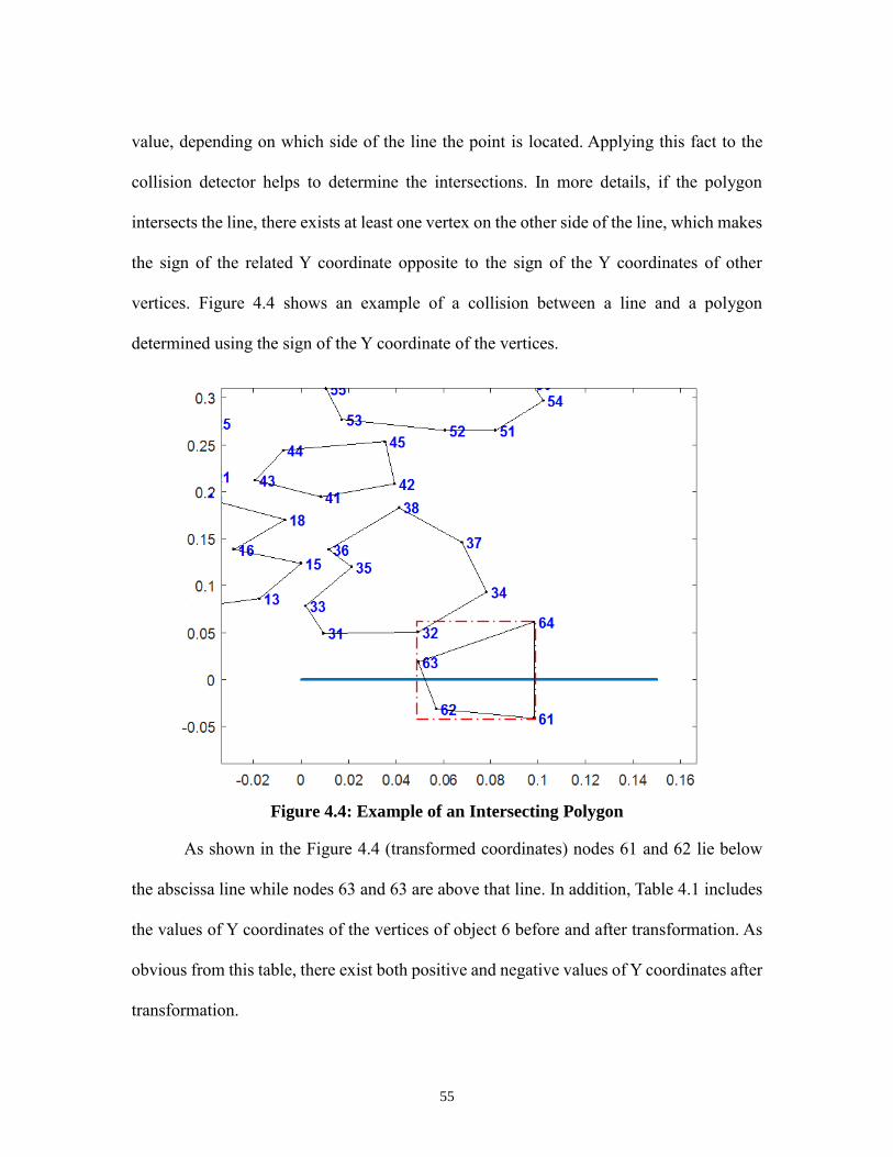
55

value, depending on which side of the line the point is located. Applying this fact to the

collision detector helps to determine the intersections. In more details, if the polygon

intersects the line, there exists at least one vertex on the other side of the line, which makes

the sign of the related Y coordinate opposite to the sign of the Y coordinates of other

vertices. Figure 4.4 shows an example of a collision between a line and a polygon

determined using the sign of the Y coordinate of the vertices.

Figure 4.4: Example of an Intersecting Polygon

As shown in the Figure 4.4 (transformed coordinates) nodes 61 and 62 lie below

the abscissa line while nodes 63 and 63 are above that line. In addition, Table 4.1 includes

the values of Y coordinates of the vertices of object 6 before and after transformation. As

obvious from this table, there exist both positive and negative values of Y coordinates after

transformation.

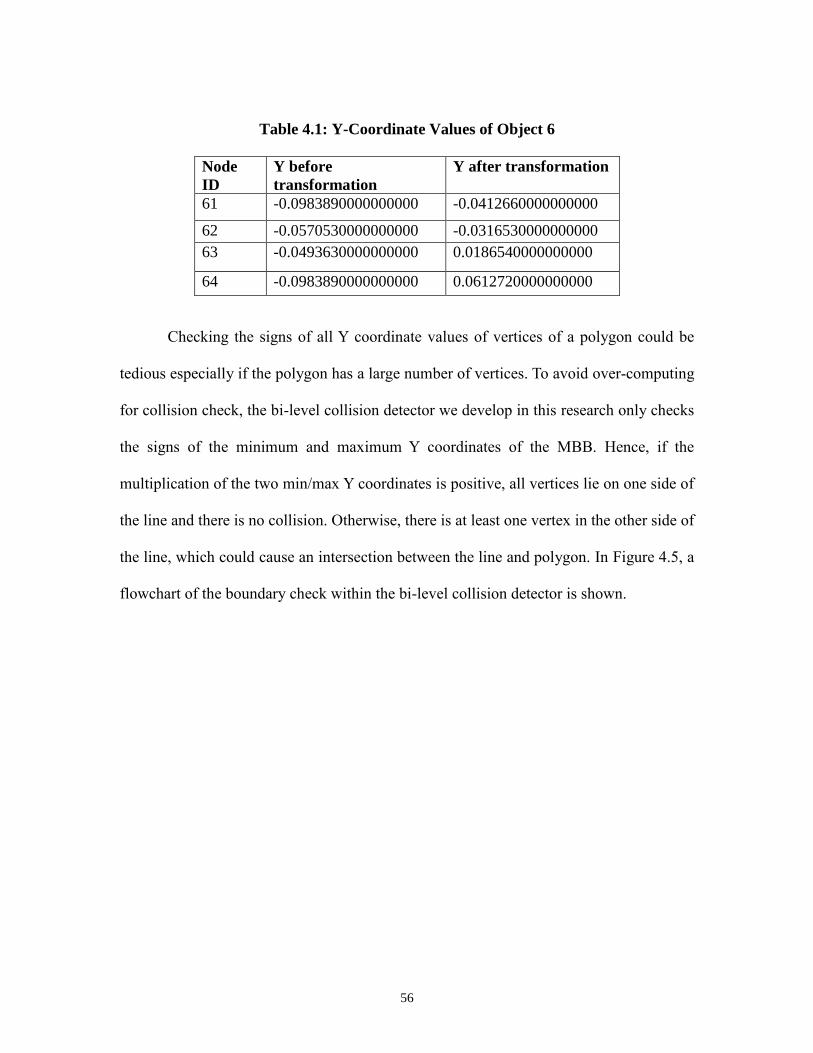
56

Table 4.1: Y-Coordinate Values of Object 6

Node

ID

Y before

transformation

Y after transformation

61 -0.0983890000000000 -0.0412660000000000

62 -0.0570530000000000 -0.0316530000000000

63 -0.0493630000000000 0.0186540000000000

64 -0.0983890000000000 0.0612720000000000

Checking the signs of all Y coordinate values of vertices of a polygon could be

tedious especially if the polygon has a large number of vertices. To avoid over-computing

for collision check, the bi-level collision detector we develop in this research only checks

the signs of the minimum and maximum Y coordinates of the MBB. Hence, if the

multiplication of the two min/max Y coordinates is positive, all vertices lie on one side of

the line and there is no collision. Otherwise, there is at least one vertex in the other side of

the line, which could cause an intersection between the line and polygon. In Figure 4.5, a

flowchart of the boundary check within the bi-level collision detector is shown.

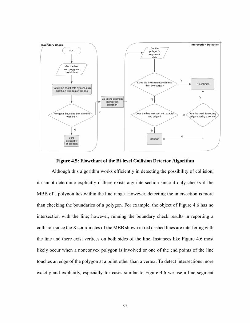
57

Start

Get the line

and polygon’s

nodal data

Rotate the coordinate system such

that the X axis lies on the line

Polygon’s bounding box interfere

with line?

zero

probability

of collision

Go to line segment

intersection

detection

Get the

polygon’s

segmental

data

Does the line intersect with less

than two edges?

Y

N

No collision

Does the line intersect with exactly

two edges?

Collision

Y

N

N

Are the two intersecting

edges sharing a vertex?

N

Y

Figure 4.5: Flowchart of the Bi-level Collision Detector Algorithm

Although this algorithm works efficiently in detecting the possibility of collision,

it cannot determine explicitly if there exists any intersection since it only checks if the

MBB of a polygon lies within the line range. However, detecting the intersection is more

than checking the boundaries of a polygon. For example, the object of Figure 4.6 has no

intersection with the line; however, running the boundary check results in reporting a

collision since the X coordinates of the MBB shown in red dashed lines are interfering with

the line and there exist vertices on both sides of the line. Instances like Figure 4.6 most

likely occur when a nonconvex polygon is involved or one of the end points of the line

touches an edge of the polygon at a point other than a vertex. To detect intersections more

exactly and explicitly, especially for cases similar to Figure 4.6 we use a line segment

58

intersection check. Thus, based on the flowchart of Figure 4.5, after determining the

possibility of collision, the problem enters the second level of the collision detector where

the polygon edges are checked for intersections with the line.

Figure 4.6: Non-intersecting Polygon with Collision Possibility

Before explaining the segment intersection detector, it is necessary to know the

basic definition of intersection. The first phase of the collision detector, boundary check,

mainly works with the coordinates of the extreme points or vertices of the polygon’s MBB

and does nothing with the polygon’s edges. However, the second phase, intersection check,

deals with the segments or edges of a polygon and checks if any segment intersects with

the line.

A line segment is a line which has two fixed endpoints. A polygon, as defined by

O’Rourke[14], is “a region of the plane bounded by a finite number of line segments”.

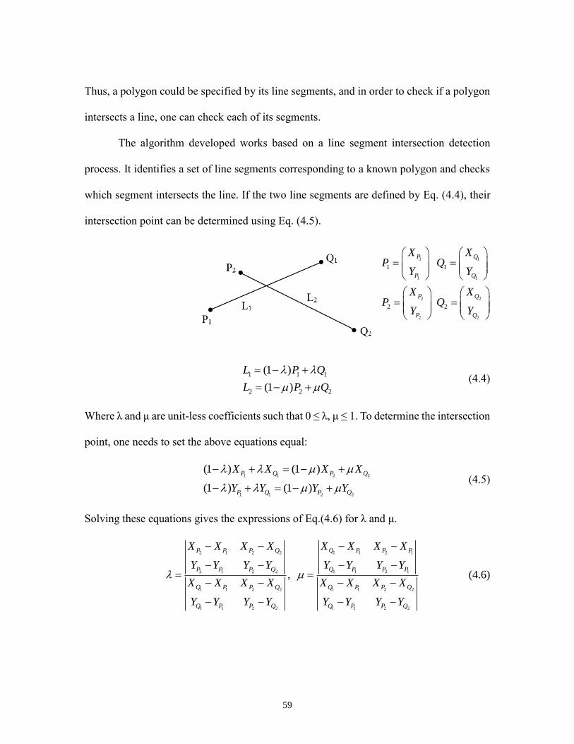
59

Thus, a polygon could be specified by its line segments, and in order to check if a polygon

intersects a line, one can check each of its segments.

The algorithm developed works based on a line segment intersection detection

process. It identifies a set of line segments corresponding to a known polygon and checks

which segment intersects the line. If the two line segments are defined by Eq. (4.4), their

intersection point can be determined using Eq. (4.5).

1 1 1

2 2 2

(1 )

(1 )

L P Q

L P Q

(4.4)

Where λ and μ are unit-less coefficients such that 0 ≤ λ, μ ≤ 1. To determine the intersection

point, one needs to set the above equations equal:

1 1 2 2

1 1 2 2

(1 ) (1 )

(1 ) (1 )

P Q P Q

P Q P Q

X X X X

Y Y Y Y

(4.5)

Solving these equations gives the expressions of Eq.(4.6) for λ and μ.

2 1 2 2 1 1 2 1

2 1 2 2 1 1 2 1

1 1 2 2 1 1 2 2

1 1 2 2 1 1 2 2

,

P P P Q Q P P P

P P P Q Q P P P

Q P P Q Q P P Q

Q P P Q Q P P Q

X X X X X X X X

Y Y Y Y Y Y Y Y

X X X X X X X X

Y Y Y Y Y Y Y Y

(4.6)

1

1

2

2

1

2

P

P

P

P

XP

Y

XP

Y

1

1

2

2

1

2

Q

Q

Q

Q

XQ

Y

XQ

Y

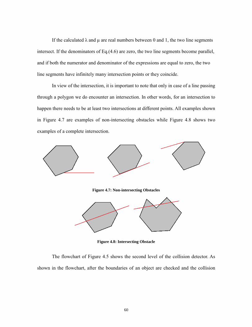
60

If the calculated λ and μ are real numbers between 0 and 1, the two line segments

intersect. If the denominators of Eq.(4.6) are zero, the two line segments become parallel,

and if both the numerator and denominator of the expressions are equal to zero, the two

line segments have infinitely many intersection points or they coincide.

In view of the intersection, it is important to note that only in case of a line passing

through a polygon we do encounter an intersection. In other words, for an intersection to

happen there needs to be at least two intersections at different points. All examples shown

in Figure 4.7 are examples of non-intersecting obstacles while Figure 4.8 shows two

examples of a complete intersection.

Figure 4.7: Non-intersecting Obstacles

Figure 4.8: Intersecting Obstacle

The flowchart of Figure 4.5 shows the second level of the collision detector. As

shown in the flowchart, after the boundaries of an object are checked and the collision

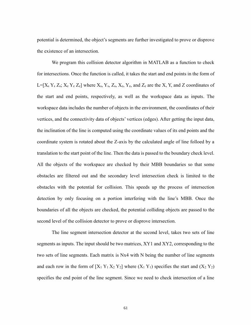
61

potential is determined, the object’s segments are further investigated to prove or disprove

the existence of an intersection.

We program this collision detector algorithm in MATLAB as a function to check

for intersections. Once the function is called, it takes the start and end points in the form of

L=[Xs Ys Zs; Xe Ye Ze] where Xs, Ys, Zs, Xe, Ye, and Ze are the X, Y, and Z coordinates of

the start and end points, respectively, as well as the workspace data as inputs. The

workspace data includes the number of objects in the environment, the coordinates of their

vertices, and the connectivity data of objects’ vertices (edges). After getting the input data,

the inclination of the line is computed using the coordinate values of its end points and the

coordinate system is rotated about the Z-axis by the calculated angle of line folloed by a

translation to the start point of the line. Then the data is passed to the boundary check level.

All the objects of the workspace are checked by their MBB boundaries so that some

obstacles are filtered out and the secondary level intersection check is limited to the

obstacles with the potential for collision. This speeds up the process of intersection

detection by only focusing on a portion interfering with the line’s MBB. Once the

boundaries of all the objects are checked, the potential colliding objects are passed to the

second level of the collision detector to prove or disprove intersection.

The line segment intersection detector at the second level, takes two sets of line

segments as inputs. The input should be two matrices, XY1 and XY2, corresponding to the

two sets of line segments. Each matrix is Nx4 with N being the number of line segments

and each row in the form of [X1 Y1 X2 Y2] where (X1 Y1) specifies the start and (X2 Y2)

specifies the end point of the line segment. Since we need to check intersection of a line

62

and a polygon, the first matrix associated with the line has a size of 1x4 while the second

matrix or the set of line segments for the polygonal obstacle has a size of Nsx4 with Ns

being the number of edges in the obstacle. After checking for segment-segment

intersections, the function outputs a 1xNs adjacency matrix which indicates the segments

in the obstacle that intersect with the line, and two 1xNs intersection matrices that include

the X and Y coordinates of the intersection point(s). Since a complete intersection happens

when a line intersects an object at (at least) two distinct points on the object’s boundary, if

the number of intersection points is greater than two, an intersection between the line and

the object is guaranteed to happen. This situation can be seen in Figure 4.8. Normally, if

the number of intersection points is greater than 2 the object is non-convex as in Figure 4.8

right. If there are exactly two intersection points, they must have different coordinates in

order for an intersection to exist, otherwise, there is no intersection. For example, in Figure

4.7 the middle and right figures show intersections at more than two points. In the figure

on the right, the line intersects two of the polygon’s edges. However, since the intersections

overlap at a vertex resulting in equal coordinates for the intersection points, this situation

is not considered as a complete intersection because the line does not pass through or

intersect the interior of the polygon. Note that the middle figure shows an intersection

situation in which a line segment intersects a polygon at more than two points the

coordinates of which are distinct. However, this object would be filtered out by the first

level of the collision detector since it lies completely on one side of the line (it only touches

the boundary and does not intersect the interior of the object) so there is no need for further

investigation of the coordinates of the intersection points. The MATLAB code for bi-level

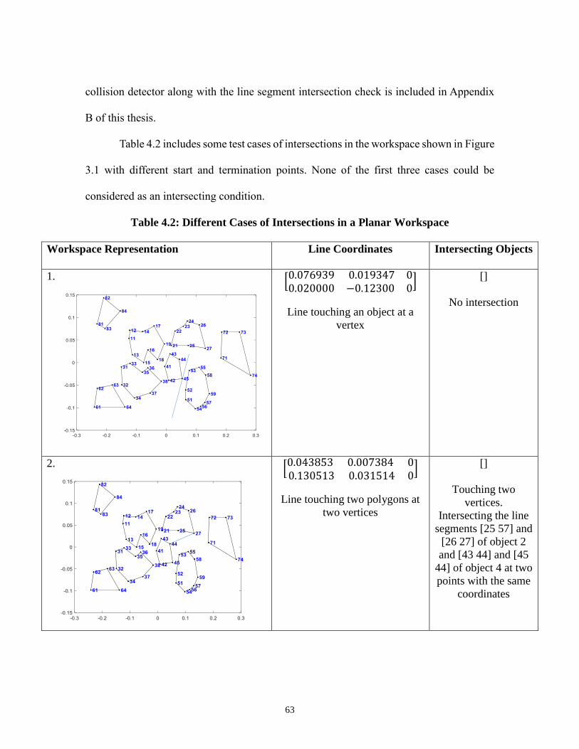
63

collision detector along with the line segment intersection check is included in Appendix

B of this thesis.

Table 4.2 includes some test cases of intersections in the workspace shown in Figure

3.1 with different start and termination points. None of the first three cases could be

considered as an intersecting condition.

Table 4.2: Different Cases of Intersections in a Planar Workspace

Workspace Representation Line Coordinates Intersecting Objects

1.

[0.076939 0.019347 00.020000 −0.12300 0

]

Line touching an object at a

vertex

[]

No intersection

2.

[0.043853 0.007384 00.130513 0.031514 0

]

Line touching two polygons at

two vertices

[]

Touching two

vertices.

Intersecting the line

segments [25 57] and

[26 27] of object 2

and [43 44] and [45

44] of object 4 at two

points with the same

coordinates

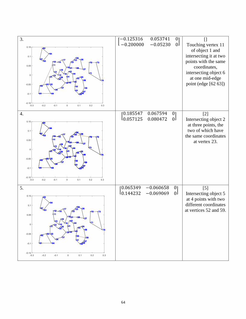
64

3.

[−0.125316 0.053741 0−0.200000 −0.05230 0

] []

Touching vertex 11

of object 1 and

intersecting it at two

points with the same

coordinates,

intersecting object 6

at one mid-edge

point (edge [62 63])

4.

[0.185547 0.067594 00.057125 0.080472 0

] [2]

Intersecting object 2

at three points, the

two of which have

the same coordinates

at vertex 23.

5.

[0.065349 −0.060658 00.144232 −0.069069 0

] [5]

Intersecting object 5

at 4 points with two

different coordinates

at vertices 52 and 59.

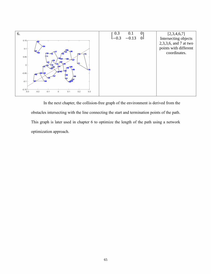
65

6.

[0.3 0.1 0

−0.3 −0.13 0] [2,3,4,6,7]

Intersecting objects

2,3,3,6, and 7 at two

points with different

coordinates.

In the next chapter, the collision-free graph of the environment is derived from the

obstacles intersecting with the line connecting the start and termination points of the path.

This graph is later used in chapter 6 to optimize the length of the path using a network

optimization approach.

66

Chapter Five

DEVELOPMENT OF THE FREE-SPACE GRAPH

Path finding in an environment is usually coupled with avoiding possible

interferences with scattered obstacles, as pointed out in the previous chapter. After

detecting such possible interferences, an approach must be taken to avoid the collisions.

One method of avoiding collision is to identify the regions of the potential intersections

and mark them as forbidden zones or to define an inclusive graph of the unoccupied space

known as the free space graph in literature. The free space graph is a graph whose edges

do not intersect the interior of any obstacles and its vertices are the obstacles’ vertices. Such

a graph would automatically handle the collision avoidance problem and all paths found

on it will be collision-free. Construction of the free space graph builds up the geometric

data structure needed for the optimization of the path. Hence, the continuous problem of

path finding in the 2D (or 3D) environment would be converted into a discrete problem of

searching a graph for the optimal, often times shortest, path between two nodes of the

graph.

In computational geometry, there are some methods of generating collision-free

graphs in a cluttered workspace to circumvent the intersection problem. These methods fall

into the category of roadmap techniques. The two most common techniques of graph

generation as noted in chapter 2 are visibility graphs and Voronoi diagrams. In addition to

the roadmap techniques, researchers employ cell decompositions to address the problem of

robot motion planning. In the following sections, we elaborate on these graph generation

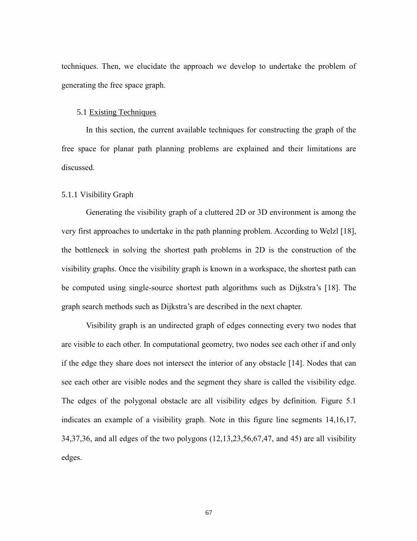
67

techniques. Then, we elucidate the approach we develop to undertake the problem of

generating the free space graph.

5.1 Existing Techniques

In this section, the current available techniques for constructing the graph of the

free space for planar path planning problems are explained and their limitations are

discussed.

5.1.1 Visibility Graph

Generating the visibility graph of a cluttered 2D or 3D environment is among the

very first approaches to undertake in the path planning problem. According to Welzl [18],

the bottleneck in solving the shortest path problems in 2D is the construction of the

visibility graphs. Once the visibility graph is known in a workspace, the shortest path can

be computed using single-source shortest path algorithms such as Dijkstra’s [18]. The

graph search methods such as Dijkstra’s are described in the next chapter.

Visibility graph is an undirected graph of edges connecting every two nodes that

are visible to each other. In computational geometry, two nodes see each other if and only

if the edge they share does not intersect the interior of any obstacle [14]. Nodes that can

see each other are visible nodes and the segment they share is called the visibility edge.

The edges of the polygonal obstacle are all visibility edges by definition. Figure 5.1

indicates an example of a visibility graph. Note in this figure line segments 14,16,17,

34,37,36, and all edges of the two polygons (12,13,23,56,67,47, and 45) are all visibility

edges.

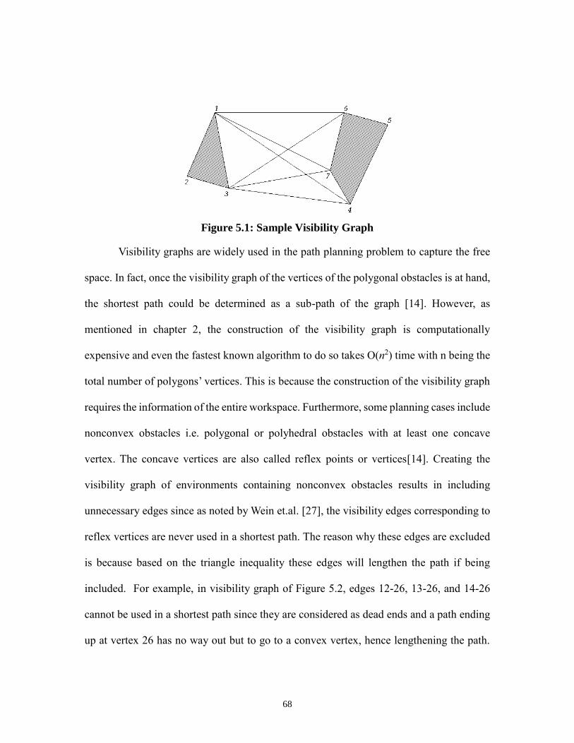
68

Figure 5.1: Sample Visibility Graph

Visibility graphs are widely used in the path planning problem to capture the free

space. In fact, once the visibility graph of the vertices of the polygonal obstacles is at hand,

the shortest path could be determined as a sub-path of the graph [14]. However, as

mentioned in chapter 2, the construction of the visibility graph is computationally

expensive and even the fastest known algorithm to do so takes O(n2) time with n being the

total number of polygons’ vertices. This is because the construction of the visibility graph

requires the information of the entire workspace. Furthermore, some planning cases include

nonconvex obstacles i.e. polygonal or polyhedral obstacles with at least one concave

vertex. The concave vertices are also called reflex points or vertices[14]. Creating the

visibility graph of environments containing nonconvex obstacles results in including

unnecessary edges since as noted by Wein et.al. [27], the visibility edges corresponding to

reflex vertices are never used in a shortest path. The reason why these edges are excluded

is because based on the triangle inequality these edges will lengthen the path if being

included. For example, in visibility graph of Figure 5.2, edges 12-26, 13-26, and 14-26

cannot be used in a shortest path since they are considered as dead ends and a path ending

up at vertex 26 has no way out but to go to a convex vertex, hence lengthening the path.

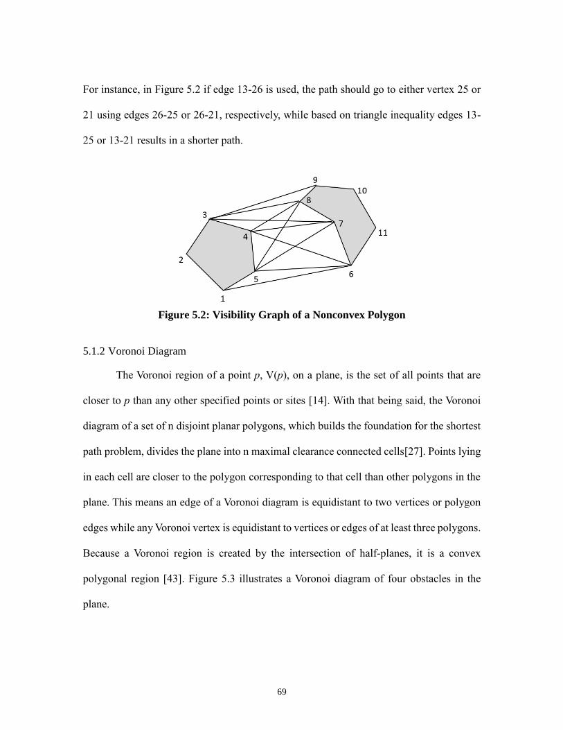
69

For instance, in Figure 5.2 if edge 13-26 is used, the path should go to either vertex 25 or

21 using edges 26-25 or 26-21, respectively, while based on triangle inequality edges 13-

25 or 13-21 results in a shorter path.

Figure 5.2: Visibility Graph of a Nonconvex Polygon

5.1.2 Voronoi Diagram

The Voronoi region of a point p, V(p), on a plane, is the set of all points that are

closer to p than any other specified points or sites [14]. With that being said, the Voronoi

diagram of a set of n disjoint planar polygons, which builds the foundation for the shortest

path problem, divides the plane into n maximal clearance connected cells[27]. Points lying

in each cell are closer to the polygon corresponding to that cell than other polygons in the

plane. This means an edge of a Voronoi diagram is equidistant to two vertices or polygon

edges while any Voronoi vertex is equidistant to vertices or edges of at least three polygons.

Because a Voronoi region is created by the intersection of half-planes, it is a convex

polygonal region [43]. Figure 5.3 illustrates a Voronoi diagram of four obstacles in the

plane.

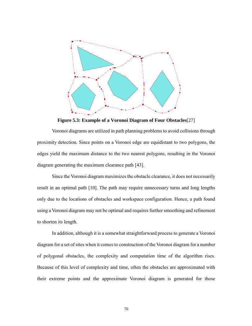
70

Figure 5.3: Example of a Voronoi Diagram of Four Obstacles[27]

Voronoi diagrams are utilized in path planning problems to avoid collisions through

proximity detection. Since points on a Voronoi edge are equidistant to two polygons, the

edges yield the maximum distance to the two nearest polygons, resulting in the Voronoi

diagram generating the maximum clearance path [43].

Since the Voronoi diagram maximizes the obstacle clearance, it does not necessarily

result in an optimal path [10]. The path may require unnecessary turns and long lengths

only due to the locations of obstacles and workspace configuration. Hence, a path found

using a Voronoi diagram may not be optimal and requires further smoothing and refinement

to shorten its length.

In addition, although it is a somewhat straightforward process to generate a Voronoi

diagram for a set of sites when it comes to construction of the Voronoi diagram for a number

of polygonal obstacles, the complexity and computation time of the algorithm rises.

Because of this level of complexity and time, often the obstacles are approximated with

their extreme points and the approximate Voronoi diagram is generated for those

71

points[44], [10]. In general, the construction of a Voronoi diagram for path planning among

polygonal obstacles requires the proximity information of the entire workspace.

Both construction of, and search in, a Voronoi diagram are faster than a visibility

graph [10]. In fact, even the fastest developed algorithm for constructing a visibility graph

[45] that takes O(n2) is much slower than constructing the Voronoi diagram for the same

environment which takes O(nlogn) time [10].

Despite the efficiency and versatility [10] of the Voronoi diagram in addressing the

path planning problem, it does not guarantee the optimality of the final solution. Besides,

the approximation of the obstacles by points is challenging and it often affects the final

solution. Last but not the least, similarly to a visibility graph, the Voronoi diagram also

requires the proximity information of the whole workspace, which may not seem effective

and fast when only a portion of the workspace may be involved in the path planning.

5.1.3 Cell Decomposition

Cell decomposition is among the first methods developed to tackle the problem of

motion planning [14]. Similar to visibility and Voronoi techniques, cell decomposition also

has its origin in computational geometry. In this method, the free space is partitioned into

a finite number of non-overlapping cells. To determine a collision-free path between the

start and end points using cell decomposition, one requires to first identify the cells

containing the start and end points. These cells are then connected using a sequence of

connected cells. Decomposition could be either exact or approximate. Approximate

decomposition is a recursive process of breaking down the free space into rectangular cells

until each cell is entirely inside an obstacle or in the free space. Recursion terminates when

72

a pre-defined accuracy of decomposition is achieved. Exact cell decomposition uses

trapezoidal and triangular cells and is often faster; nevertheless, the solution is not optimal.

However, upon increasing the accuracy of the approximate cell decomposition(decreasing

the cell size), near-optimal solutions are achievable at the cost of longer computation time

[10].

In all the aforementioned roadmap techniques, the entire environment’s information

is required to be able to construct a graph of the workspace. Nevertheless, there might be

cases in which a portion of the environment comprised of a subset of obstacles is involved

in the path-finding problem. Thus, restricting the construction and search processes to that

specific portion should help to simplify the problem by eliminating the complexities and

speeding up the path-planning algorithm.

Based on this, we propose a method to capture the free space graph using the convex

hulls of the intersecting obstacles that are detected from employing the bi-level intersection

detector. In the next section, the details of this method are provided.

5.2 Proposed Approach: Planning based on the convex hulls of the obstacles

In order to speed up the path-planning algorithm, simplify the complexities that lie

in roadmap techniques, and to come up with an optimal rather than near-optimal solution

to the 2D path-planning problem, we underlie our technique based on the notion of convex

hulls of the obstacles. Convex hulls have properties that are important in finding the

shortest path. For example, in [23] the authors claim that the shortest path in the TSP

problem passes through the convex hull of the cities. Also, as pointed out by Wein [27], the

shortest paths in a cluttered environment are tangent to the obstacles (the proof of which is

73

simple using the triangle inequality). Since by definition the convex hull of an object is the

smallest enclosure containing the object, hence including tangent edges to the obstacles, it

could be used to determine the shortest path. Based upon these properties of the convex

hulls, we develop an efficient algorithm to find the free space graph of the environment.

In our proposed approach, instead of capturing the free space using the information

from the entire workspace, we limit our scope to that portion of the workspace interfering

with the shortest straight line connecting the start and end points. Since the straight line is

the shortest path between two points regardless of colliding the obstacles, it is set as the

reference line of our algorithm. The closer the router moves towards the reference line, the

shorter the path is to reach the goal. Hence, instead of planning the path as far as possible

from the obstacles, unlike the Voronoi diagrams, we attempt to keep it close to the obstacles

such that it touches them but not intersect their interior. Consequently, the obstacles

detected to be intersecting, using the bi-level intersection detector, are the foundations of

this approach. In the next section, the construction of the free space graph based on convex

hulls is explained.

5.2.1 Free space graph formation

Suppose we denote the workspace by W, since we are looking at solving the

problem in a 2D environment, we know that:

𝑊 ⊆ ℝ2

Now, suppose there are n polygonal obstacles, Pi , (i = 1, 2, …, n) scattered in the

workspace. The geometry and location of each of the obstacles are known and they are all

stationary and disjoint. In addition, the coordinates of the start and end points of the path

74

of interest are given. The problem is to construct the free space defined as Eq.(5.1) in the

form of a graph.

1

\ iee

n

f

i

r PC W

(5.1)

In Eq.(5.1) Cfree denotes the free space as a subset of the workspace which could be

generated by subtracting the union of all occupied spaces by the obstacles from the

workspace. The graph G to be constructed from the free space is defined as follows by its

set of vertices (V) and edges (E).

𝐺 ⊆ 𝐶𝑓𝑟𝑒𝑒 , 𝐺 = {𝑉, 𝐸} (5.2)

Now, we need to find this graph such that its edges do not intersect the interior of

any of the obstacles. To find this graph means to determine its vertices and edges.

Assuming there is only one obstacle in the workspace, one needs to determine if

the path connecting the start (A) and termination (B) points intersects the interior of the

obstacle. By definition, the convex hull of a set of points is the smallest convex set

containing all points. The convex hull of two points, by this definition, is the line

connecting the points. Thus, we confirm the intersection between a line segment (AB) and

a polygon (P) if the condition below holds:

𝐶𝑜𝑛𝑣(𝐴, 𝐵) ∩ 𝑃 ⊂ 𝑖𝑛𝑡(𝑃) ∪ 𝜕(𝑃) (5.3)

Where Conv(A,B) is the convex hull of the two points A and B, P is the polygonal

obstacle in the workspace, 𝑃 ⊂ 𝑊, int(P) denotes the interior of the polygon P, and 𝜕(𝑃)

is the boundary of the polygon P as could be seen in Figure 5.4.

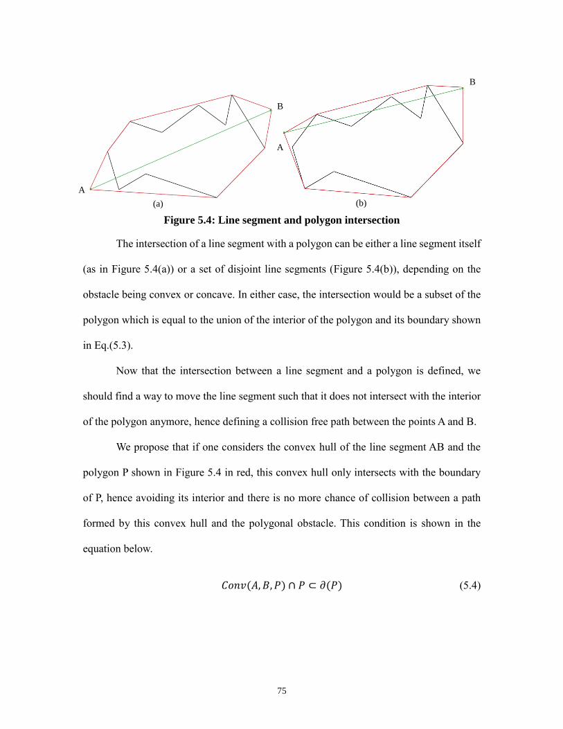
75

Figure 5.4: Line segment and polygon intersection

The intersection of a line segment with a polygon can be either a line segment itself

(as in Figure 5.4(a)) or a set of disjoint line segments (Figure 5.4(b)), depending on the

obstacle being convex or concave. In either case, the intersection would be a subset of the

polygon which is equal to the union of the interior of the polygon and its boundary shown

in Eq.(5.3).

Now that the intersection between a line segment and a polygon is defined, we

should find a way to move the line segment such that it does not intersect with the interior

of the polygon anymore, hence defining a collision free path between the points A and B.

We propose that if one considers the convex hull of the line segment AB and the

polygon P shown in Figure 5.4 in red, this convex hull only intersects with the boundary

of P, hence avoiding its interior and there is no more chance of collision between a path

formed by this convex hull and the polygonal obstacle. This condition is shown in the

equation below.

𝐶𝑜𝑛𝑣(𝐴, 𝐵, 𝑃) ∩ 𝑃 ⊂ 𝜕(𝑃) (5.4)

A

A

B

B

(a) (b)

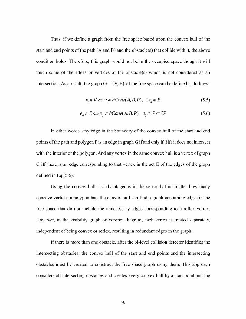
76

Thus, if we define a graph from the free space based upon the convex hull of the

start and end points of the path (A and B) and the obstacle(s) that collide with it, the above

condition holds. Therefore, this graph would not be in the occupied space though it will

touch some of the edges or vertices of the obstacle(s) which is not considered as an

intersection. As a result, the graph G = {V, E} of the free space can be defined as follows:

( , , ), i i ijv V v Conv A B P e E (5.5)

( , , ), ij ij ije E e Conv A B P e P P (5.6)

In other words, any edge in the boundary of the convex hull of the start and end

points of the path and polygon P is an edge in graph G if and only if (iff) it does not intersect

with the interior of the polygon. And any vertex in the same convex hull is a vertex of graph

G iff there is an edge corresponding to that vertex in the set E of the edges of the graph

defined in Eq.(5.6).

Using the convex hulls is advantageous in the sense that no matter how many

concave vertices a polygon has, the convex hull can find a graph containing edges in the

free space that do not include the unnecessary edges corresponding to a reflex vertex.

However, in the visibility graph or Voronoi diagram, each vertex is treated separately,

independent of being convex or reflex, resulting in redundant edges in the graph.

If there is more than one obstacle, after the bi-level collision detector identifies the

intersecting obstacles, the convex hull of the start and end points and the intersecting

obstacles must be created to construct the free space graph using them. This approach

considers all intersecting obstacles and creates every convex hull by a start point and the

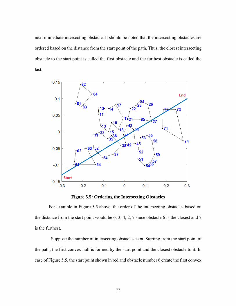
77

next immediate intersecting obstacle. It should be noted that the intersecting obstacles are

ordered based on the distance from the start point of the path. Thus, the closest intersecting

obstacle to the start point is called the first obstacle and the furthest obstacle is called the

last.

Figure 5.5: Ordering the Intersecting Obstacles

For example in Figure 5.5 above, the order of the intersecting obstacles based on

the distance from the start point would be 6, 3, 4, 2, 7 since obstacle 6 is the closest and 7

is the furthest.

Suppose the number of intersecting obstacles is m. Starting from the start point of

the path, the first convex hull is formed by the start point and the closest obstacle to it. In

case of Figure 5.5, the start point shown in red and obstacle number 6 create the first convex

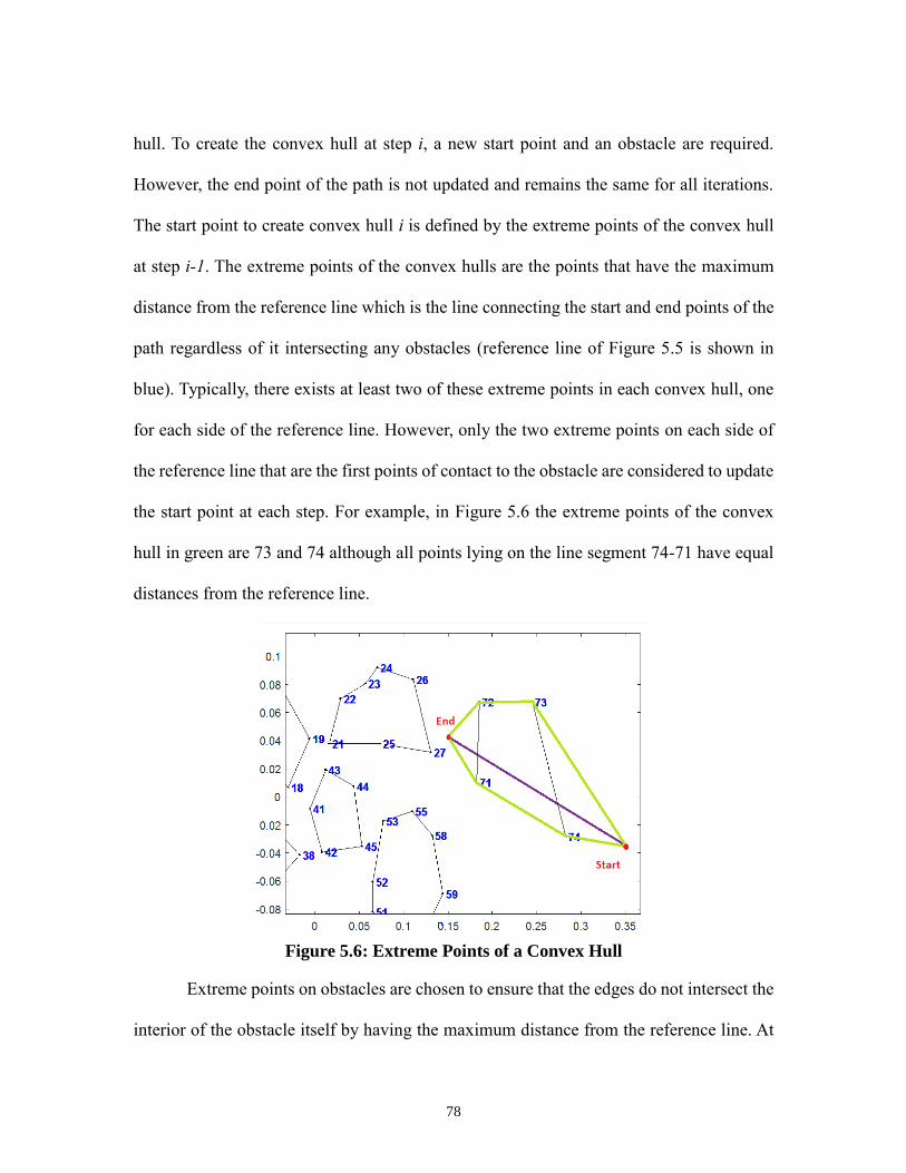
78

hull. To create the convex hull at step i, a new start point and an obstacle are required.

However, the end point of the path is not updated and remains the same for all iterations.

The start point to create convex hull i is defined by the extreme points of the convex hull

at step i-1. The extreme points of the convex hulls are the points that have the maximum

distance from the reference line which is the line connecting the start and end points of the

path regardless of it intersecting any obstacles (reference line of Figure 5.5 is shown in

blue). Typically, there exists at least two of these extreme points in each convex hull, one

for each side of the reference line. However, only the two extreme points on each side of

the reference line that are the first points of contact to the obstacle are considered to update

the start point at each step. For example, in Figure 5.6 the extreme points of the convex

hull in green are 73 and 74 although all points lying on the line segment 74-71 have equal

distances from the reference line.

Figure 5.6: Extreme Points of a Convex Hull

Extreme points on obstacles are chosen to ensure that the edges do not intersect the

interior of the obstacle itself by having the maximum distance from the reference line. At

79

each step of this approach, two convex hulls are created corresponding to the two extreme

points, except at the first and last step. At the last step, the convex hull of the last

intersecting obstacle and the end point of the path is created. Hence, for m intersecting

obstacles 2(m-1) +2 or 2m convex hulls will be created. Figure 5.7 depicts a schematic of

creating the convex hulls for 4 intersecting obstacles. Note that a total of 8 convex hulls

are created in this example.

Figure 5.7: Schematic of the First Iteration in Construction of the Free Space Graph

An edge of the convex hull is added to the graph provided it does not intersect any

obstacles. Otherwise, the process of convex hull generation is performed recursively, with

the new reference line being the edge that has an intersection until the edge is collision free

and could be added to the graph. For example, in Figure 5.7 edges 62-34, 31-42, 31-43, 37-

43, and 45-21 indicate intersections with obstacles and need be re-routed using the same

Start

End

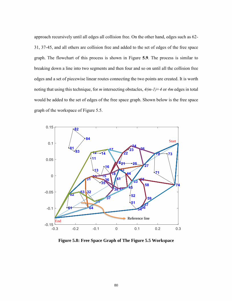
80

approach recursively until all edges all collision free. On the other hand, edges such as 62-

31, 37-45, and all others are collision free and added to the set of edges of the free space

graph. The flowchart of this process is shown in Figure 5.9. The process is similar to

breaking down a line into two segments and then four and so on until all the collision free

edges and a set of piecewise linear routes connecting the two points are created. It is worth

noting that using this technique, for m intersecting obstacles, 4(m-1)+4 or 4m edges in total

would be added to the set of edges of the free space graph. Shown below is the free space

graph of the workspace of Figure 5.5.

Figure 5.8: Free Space Graph of The Figure 5.5 Workspace

Reference line End

Start

81

This approach can be applied to any pairs of points in the workspace and the result

is an undirected graph of all collision free paths. After the graph is generated, any of the

network optimization algorithms can be implemented to optimize the path for different

optimization criteria, the most common of which is to find the shortest path. Network

optimization and solution of the shortest path problem are discussed in the next chapter.

It is worth noting that since this graph highly depends on the start and end nodes,

different graphs would be constructed for different pairs of nodes and there does not exist

a unique graph of the entire workspace unlike visibility and Voronoi; therefore, limiting

the search to a portion of the workspace which expedites the search for the shortest path.

In addition, the final solution will be the optimal path and there is no need to

approximate the obstacles and other elements of the workspace to come up with a solution.

In Table 5.1, the free space graphs of the sample workspaces from Table 4.2 in chapter 3

are constructed using the proposed technique. The time complexity of this algorithm is

derived in chapter 7.

Note that in cases 1 to 3 of Table 5.1, since the straight line connecting the start

and end points of the path does not intersect any obstacle, the shortest path between the

two points is the line itself and so is the free space graph of the workspace.

In case 4, the straight line connecting the start and end points passes through

obstacle number 5. Hence, a convex hull containing this obstacle is generated and the free

space graph is extracted from that convex hull. Since the path has end points lying on the

obstacle and only intersects that obstacle, the edges of the graph are the edges of the 5th

obstacle.

82

In case 5, the path has intersection with obstacles 1, 2, 3, 4, 5, 6, and 7. Thus, the

required convex hulls are formed and the edges of the free space graph are extracted. One

should note that in the beginning, only obstacles number 6, 3, 4, 2, and 7 intersect with the

straight line connecting the start and end point. However, as the path is re-routed to avoid

collisions, it encounters new obstacles on the way and the resulting collisions need be

avoided by creating new convex hulls containing new intersecting obstacles.

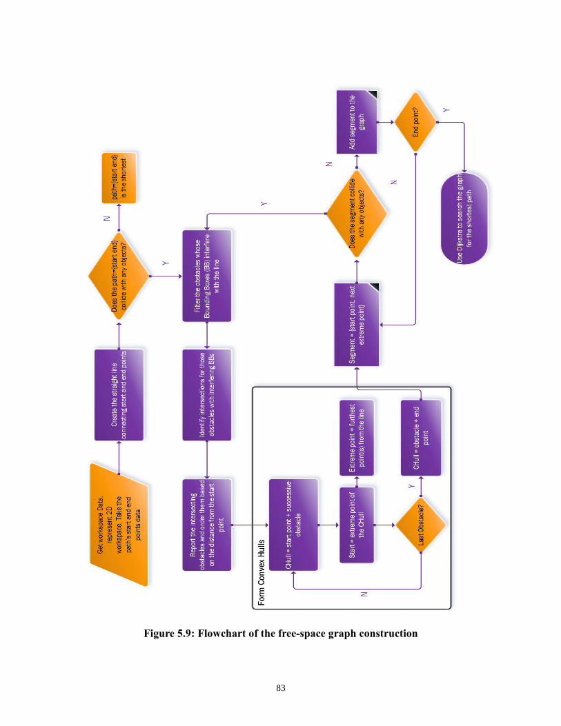
83

Figure 5.9: Flowchart of the free-space graph construction

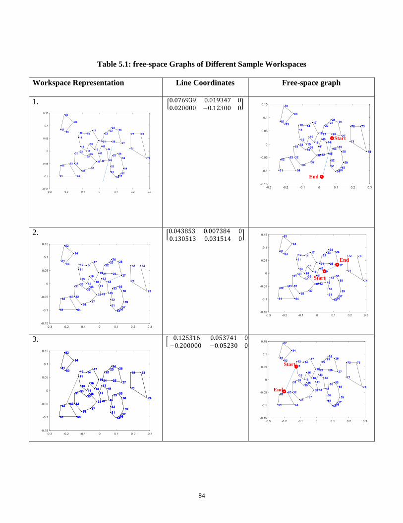
84

Table 5.1: free-space Graphs of Different Sample Workspaces

Workspace Representation Line Coordinates Free-space graph

1.

[0.076939 0.019347 00.020000 −0.12300 0

]

2.

[0.043853 0.007384 00.130513 0.031514 0

]

3.

[−0.125316 0.053741 0−0.200000 −0.05230 0

]

Start

End

End

End

Start

Start

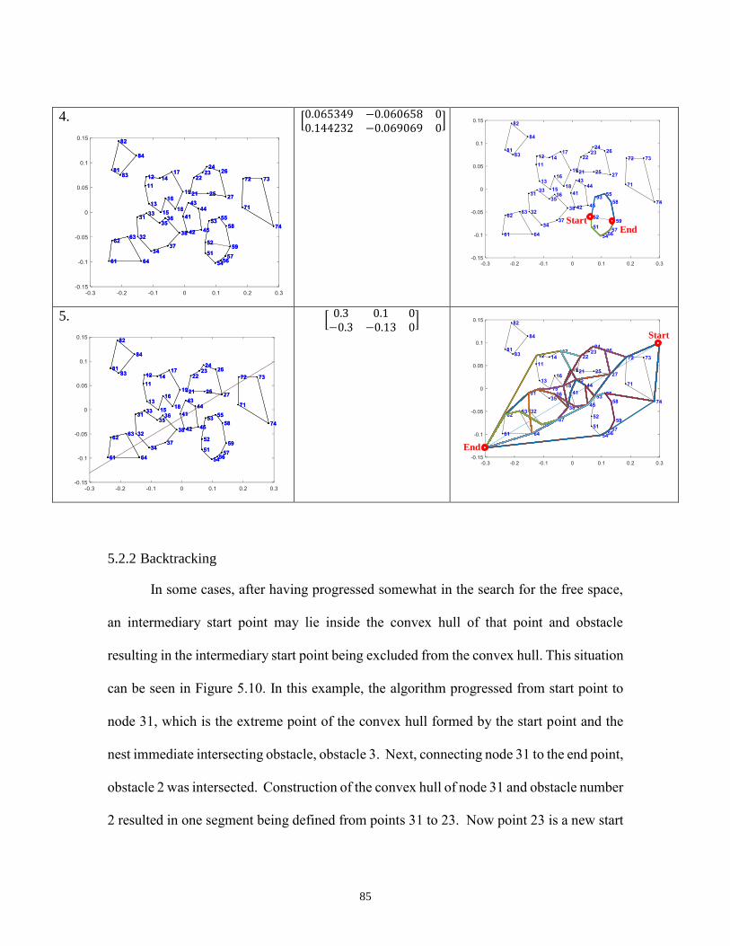
85

4.

[0.065349 −0.060658 00.144232 −0.069069 0

]

5.

[0.3 0.1 0

−0.3 −0.13 0]

5.2.2 Backtracking

In some cases, after having progressed somewhat in the search for the free space,

an intermediary start point may lie inside the convex hull of that point and obstacle

resulting in the intermediary start point being excluded from the convex hull. This situation

can be seen in Figure 5.10. In this example, the algorithm progressed from start point to

node 31, which is the extreme point of the convex hull formed by the start point and the

nest immediate intersecting obstacle, obstacle 3. Next, connecting node 31 to the end point,

obstacle 2 was intersected. Construction of the convex hull of node 31 and obstacle number

2 resulted in one segment being defined from points 31 to 23. Now point 23 is a new start

End

End

Start

Start

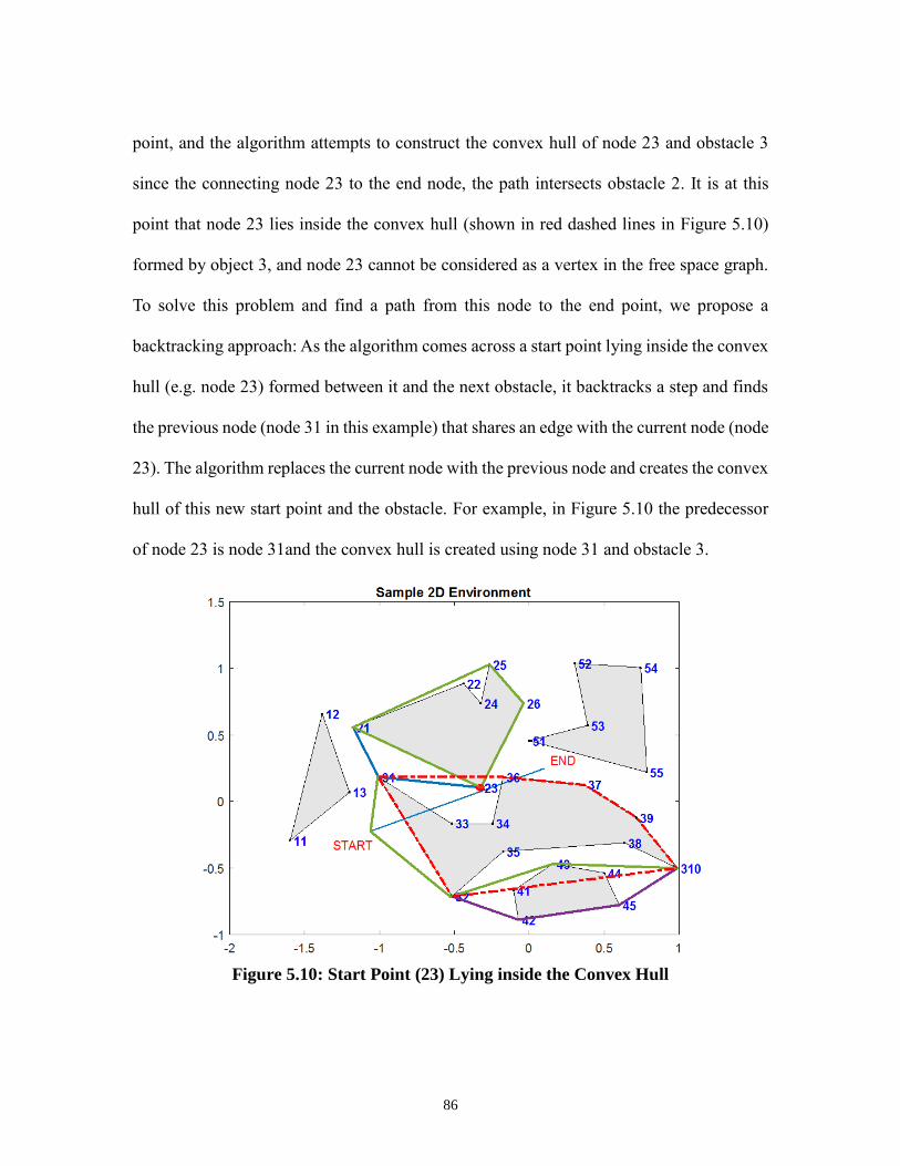
86

point, and the algorithm attempts to construct the convex hull of node 23 and obstacle 3

since the connecting node 23 to the end node, the path intersects obstacle 2. It is at this

point that node 23 lies inside the convex hull (shown in red dashed lines in Figure 5.10)

formed by object 3, and node 23 cannot be considered as a vertex in the free space graph.

To solve this problem and find a path from this node to the end point, we propose a

backtracking approach: As the algorithm comes across a start point lying inside the convex

hull (e.g. node 23) formed between it and the next obstacle, it backtracks a step and finds

the previous node (node 31 in this example) that shares an edge with the current node (node

23). The algorithm replaces the current node with the previous node and creates the convex

hull of this new start point and the obstacle. For example, in Figure 5.10 the predecessor

of node 23 is node 31and the convex hull is created using node 31 and obstacle 3.

Figure 5.10: Start Point (23) Lying inside the Convex Hull

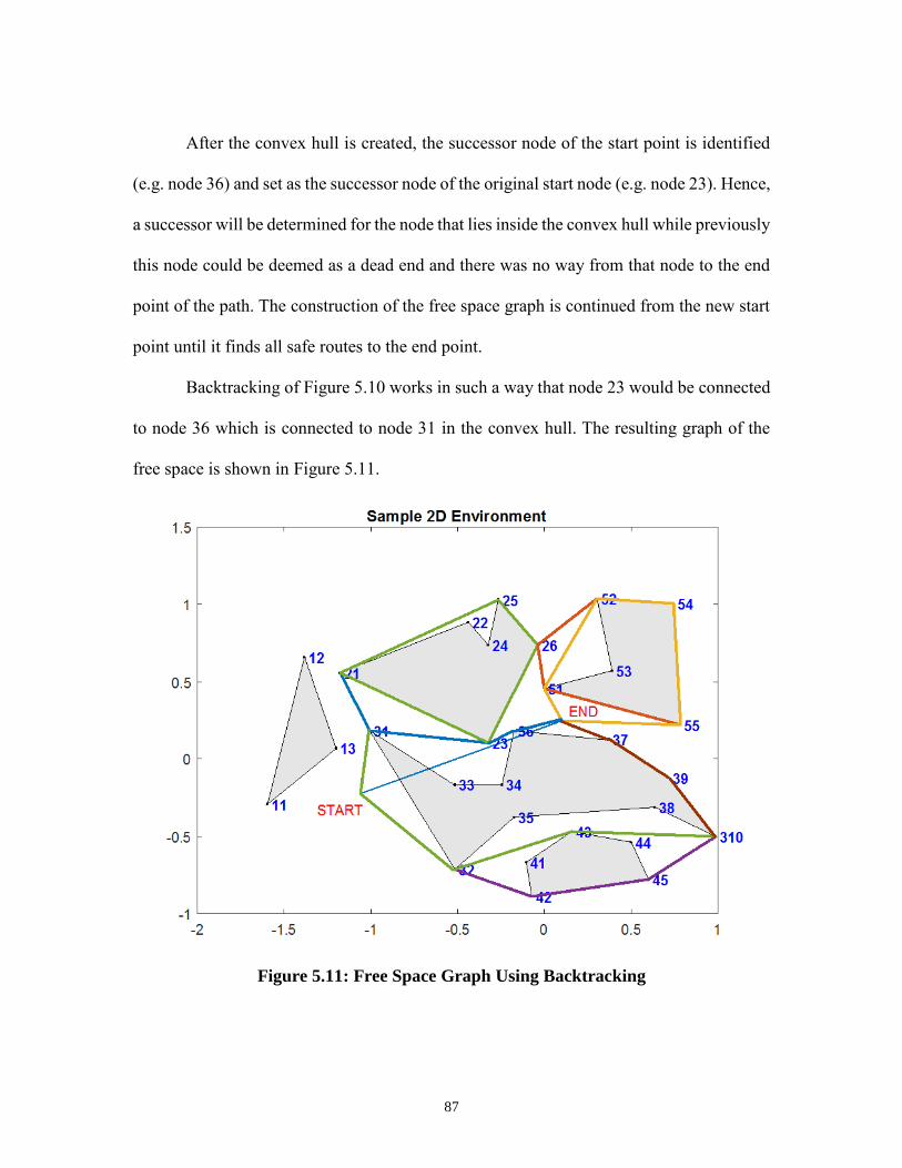
87

After the convex hull is created, the successor node of the start point is identified

(e.g. node 36) and set as the successor node of the original start node (e.g. node 23). Hence,

a successor will be determined for the node that lies inside the convex hull while previously

this node could be deemed as a dead end and there was no way from that node to the end

point of the path. The construction of the free space graph is continued from the new start

point until it finds all safe routes to the end point.

Backtracking of Figure 5.10 works in such a way that node 23 would be connected

to node 36 which is connected to node 31 in the convex hull. The resulting graph of the

free space is shown in Figure 5.11.

Figure 5.11: Free Space Graph Using Backtracking

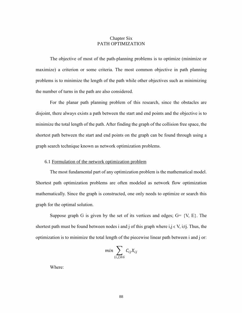
88

Chapter Six

PATH OPTIMIZATION

The objective of most of the path-planning problems is to optimize (minimize or

maximize) a criterion or some criteria. The most common objective in path planning

problems is to minimize the length of the path while other objectives such as minimizing

the number of turns in the path are also considered.

For the planar path planning problem of this research, since the obstacles are

disjoint, there always exists a path between the start and end points and the objective is to

minimize the total length of the path. After finding the graph of the collision free space, the

shortest path between the start and end points on the graph can be found through using a

graph search technique known as network optimization problems.

6.1 Formulation of the network optimization problem

The most fundamental part of any optimization problem is the mathematical model.

Shortest path optimization problems are often modeled as network flow optimization

mathematically. Since the graph is constructed, one only needs to optimize or search this

graph for the optimal solution.

Suppose graph G is given by the set of its vertices and edges; G= {V, E}. The

shortest path must be found between nodes i and j of this graph where i,j ϵ V, i≠j. Thus, the

optimization is to minimize the total length of the piecewise linear path between i and j or:

𝑚𝑖𝑛 ∑ 𝐶𝑖𝑗𝑋𝑖𝑗

(𝑖,𝑗)∈𝐺

Where:

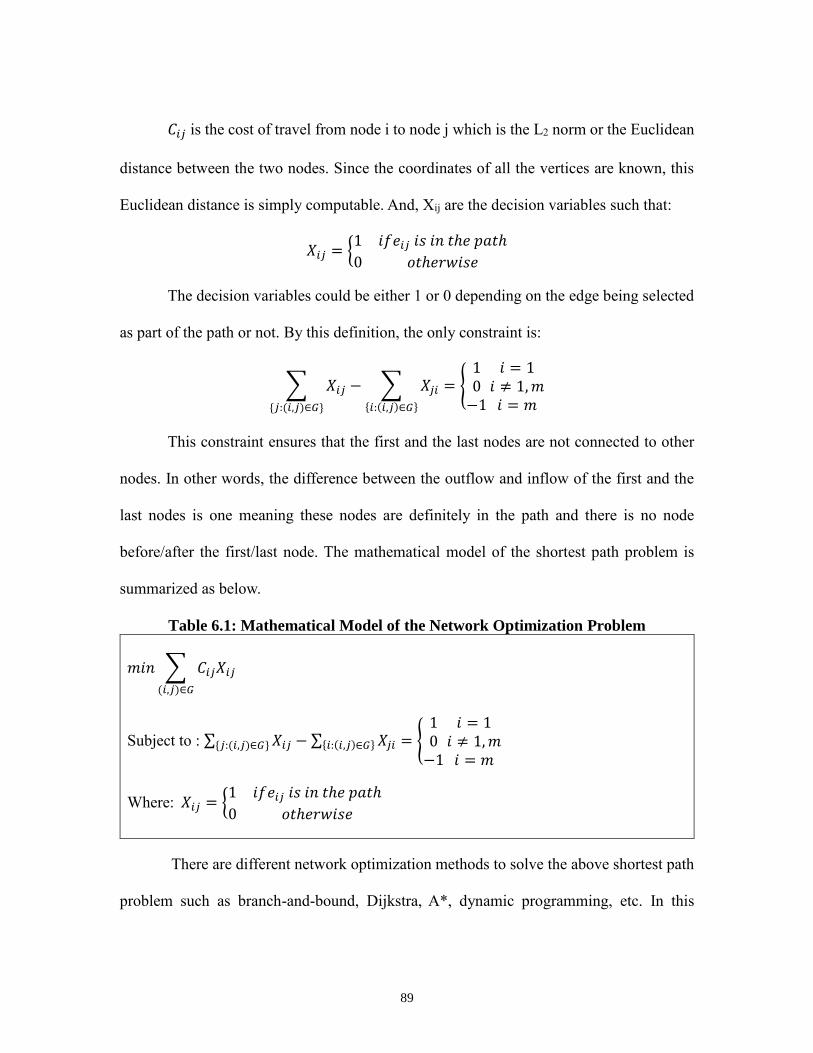
89

𝐶𝑖𝑗 is the cost of travel from node i to node j which is the L2 norm or the Euclidean

distance between the two nodes. Since the coordinates of all the vertices are known, this

Euclidean distance is simply computable. And, Xij are the decision variables such that:

𝑋𝑖𝑗 = {1 𝑖𝑓𝑒𝑖𝑗 𝑖𝑠 𝑖𝑛 𝑡ℎ𝑒 𝑝𝑎𝑡ℎ

0 𝑜𝑡ℎ𝑒𝑟𝑤𝑖𝑠𝑒

The decision variables could be either 1 or 0 depending on the edge being selected

as part of the path or not. By this definition, the only constraint is:

∑ 𝑋𝑖𝑗

{𝑗:(𝑖,𝑗)∈𝐺}

− ∑ 𝑋𝑗𝑖

{𝑖:(𝑖,𝑗)∈𝐺}

= {10

−1

𝑖 = 1𝑖 ≠ 1, 𝑚

𝑖 = 𝑚

This constraint ensures that the first and the last nodes are not connected to other

nodes. In other words, the difference between the outflow and inflow of the first and the

last nodes is one meaning these nodes are definitely in the path and there is no node

before/after the first/last node. The mathematical model of the shortest path problem is

summarized as below.

Table 6.1: Mathematical Model of the Network Optimization Problem

𝑚𝑖𝑛 ∑ 𝐶𝑖𝑗𝑋𝑖𝑗

(𝑖,𝑗)∈𝐺

Subject to : ∑ 𝑋𝑖𝑗{𝑗:(𝑖,𝑗)∈𝐺} − ∑ 𝑋𝑗𝑖{𝑖:(𝑖,𝑗)∈𝐺} = {10

−1

𝑖 = 1𝑖 ≠ 1, 𝑚

𝑖 = 𝑚

Where: 𝑋𝑖𝑗 = {1 𝑖𝑓𝑒𝑖𝑗 𝑖𝑠 𝑖𝑛 𝑡ℎ𝑒 𝑝𝑎𝑡ℎ

0 𝑜𝑡ℎ𝑒𝑟𝑤𝑖𝑠𝑒

There are different network optimization methods to solve the above shortest path

problem such as branch-and-bound, Dijkstra, A*, dynamic programming, etc. In this

90

chapter, two of the most commonly used local search algorithms are described: Dijkstra

and A*. Both algorithms work with predefined graphs. We use the free space graph

constructed in the previous chapter as the input to the search algorithm.

6.2 Dijkstra’s Shortest Path Algorithm

Dijkstra is an algorithm developed by Edsger Dijkstra [26] to find the shortest path

from a single source to one or all other nodes of a given weighted graph consists of a finite

number of nodes. The weights are non-negative numbers assigned to each edge of the

graph. For instance, weights can be the lengths of the edges of the graph or the Euclidean

distance between the two adjacent nodes of the graph connected by an edge. It is important

to note that the source node is single but the destination can be any or all other nodes of

the graph.

Dijkstra’s algorithm constitutes a tree of edges, which link the start point to the end

point in several steps. In the beginning, all nodes are divided into two sets a set of visited

(or predecessor[46]) and a set of unvisited (or successor[46]) nodes. Hence, initially, all

nodes belong to the set of unvisited nodes except the source node. In addition, a tentative

cost of ∞ is assigned to each edge, which is updated later on. Starting from the start point,

at each step, the algorithm explores all the adjacent unvisited nodes, excludes them from

the set of unvisited nodes, and updates their cost by their distance from the start point. It

then adds the node with the smallest cost to the path and sets its cost to permanent. This

node designates the current node for the next iteration. This process is repeated iteratively

until it eventually reaches the goal node. A pseudo code of this algorithm written by

Sniedovich [46] is as shown in Table 6.2.

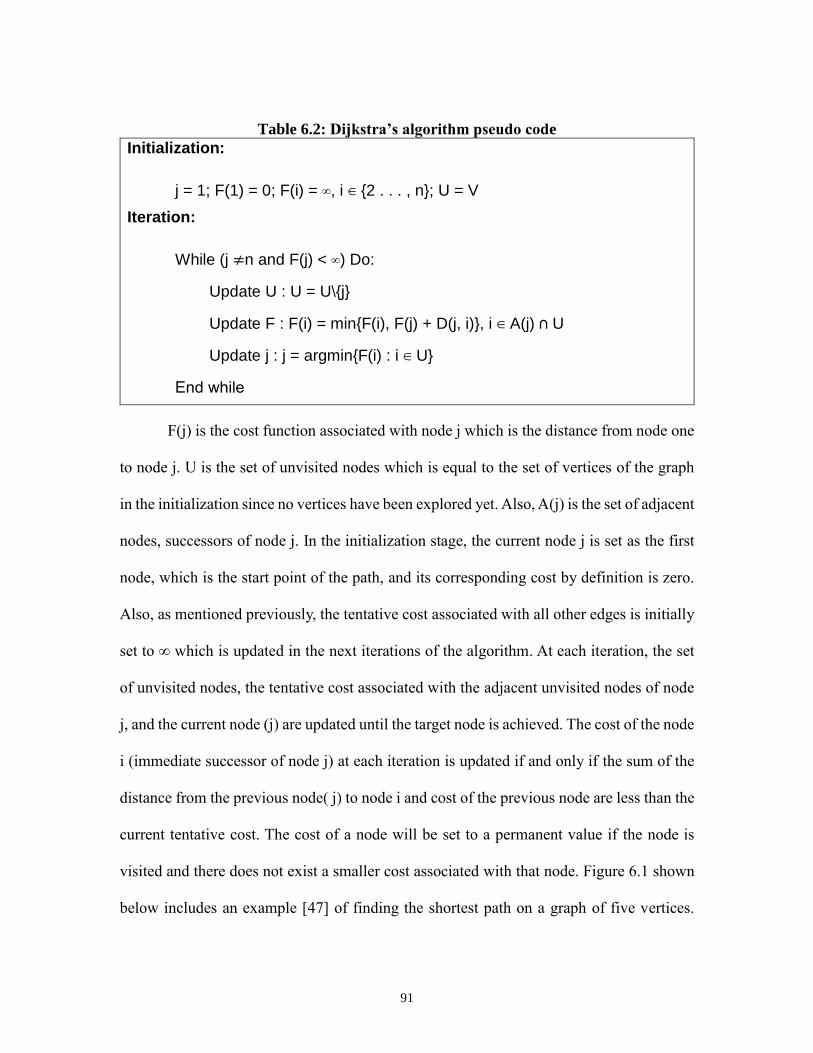
91

Table 6.2: Dijkstra’s algorithm pseudo code

Initialization:

j = 1; F(1) = 0; F(i) = ∞, i ∈ {2 . . . , n}; U = V

Iteration:

While (j ≠n and F(j) < ∞) Do:

Update U : U = U\{j}

Update F : F(i) = min{F(i), F(j) + D(j, i)}, i ∈ A(j) ∩ U

Update j : j = argmin{F(i) : i ∈ U}

End while

F(j) is the cost function associated with node j which is the distance from node one

to node j. U is the set of unvisited nodes which is equal to the set of vertices of the graph

in the initialization since no vertices have been explored yet. Also, A(j) is the set of adjacent

nodes, successors of node j. In the initialization stage, the current node j is set as the first

node, which is the start point of the path, and its corresponding cost by definition is zero.

Also, as mentioned previously, the tentative cost associated with all other edges is initially

set to ∞ which is updated in the next iterations of the algorithm. At each iteration, the set

of unvisited nodes, the tentative cost associated with the adjacent unvisited nodes of node

j, and the current node (j) are updated until the target node is achieved. The cost of the node

i (immediate successor of node j) at each iteration is updated if and only if the sum of the

distance from the previous node( j) to node i and cost of the previous node are less than the

current tentative cost. The cost of a node will be set to a permanent value if the node is

visited and there does not exist a smaller cost associated with that node. Figure 6.1 shown

below includes an example [47] of finding the shortest path on a graph of five vertices.

92

This example is from Dr. Angelia Nedich’s lecture notes on “Operations Research

Methods”.

a) Given the graph

b) Initialization

Figure 6.1: Dijkstra’s Initialization

Figure 6.1a shows the given graph of five vertices with known costs on the edges

(length of each edge). The goal is to find the shortest path from node 1 to node 5. Figure

6.1b depicts the initialization step of the Dijkstra’s algorithm. Note that in the initialization

all the costs to reach the unvisited nodes are tentative, designated by t, while node 1 has a

permanent cost of zero, designated by (0,p).

The first iteration of the Dijkstra is shown in Figure 6.2. In this iteration, nodes 2,3,

and 6 that are adjacent to node 1 and are all unvisited are explored. Note that the costs

associated with these nodes (cost of travel from node 1 to these nodes) are updated since

at node 2: 0+7 < ∞, at node 3: 0+9 < ∞, and at node 6: 0+14 < ∞. However, only the cost

of node 2 is permanent and the rest are still tentative because node 2 has the minimum cost

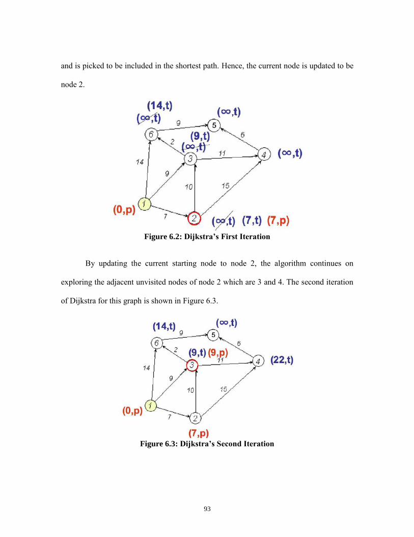
93

and is picked to be included in the shortest path. Hence, the current node is updated to be

node 2.

Figure 6.2: Dijkstra’s First Iteration

By updating the current starting node to node 2, the algorithm continues on

exploring the adjacent unvisited nodes of node 2 which are 3 and 4. The second iteration

of Dijkstra for this graph is shown in Figure 6.3.

Figure 6.3: Dijkstra’s Second Iteration

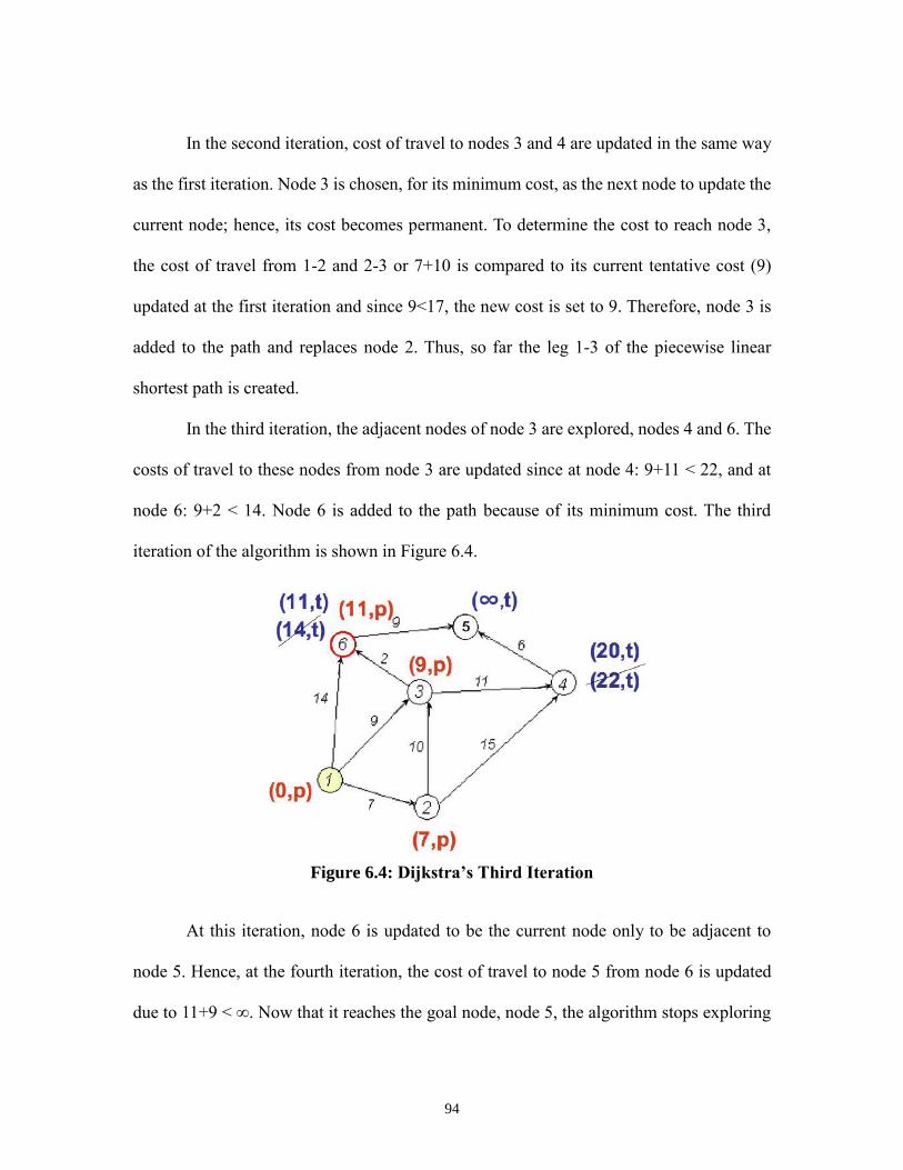
94

In the second iteration, cost of travel to nodes 3 and 4 are updated in the same way

as the first iteration. Node 3 is chosen, for its minimum cost, as the next node to update the

current node; hence, its cost becomes permanent. To determine the cost to reach node 3,

the cost of travel from 1-2 and 2-3 or 7+10 is compared to its current tentative cost (9)

updated at the first iteration and since 9<17, the new cost is set to 9. Therefore, node 3 is

added to the path and replaces node 2. Thus, so far the leg 1-3 of the piecewise linear

shortest path is created.

In the third iteration, the adjacent nodes of node 3 are explored, nodes 4 and 6. The

costs of travel to these nodes from node 3 are updated since at node 4: 9+11 < 22, and at

node 6: 9+2 < 14. Node 6 is added to the path because of its minimum cost. The third

iteration of the algorithm is shown in Figure 6.4.

Figure 6.4: Dijkstra’s Third Iteration

At this iteration, node 6 is updated to be the current node only to be adjacent to

node 5. Hence, at the fourth iteration, the cost of travel to node 5 from node 6 is updated

due to 11+9 < ∞. Now that it reaches the goal node, node 5, the algorithm stops exploring

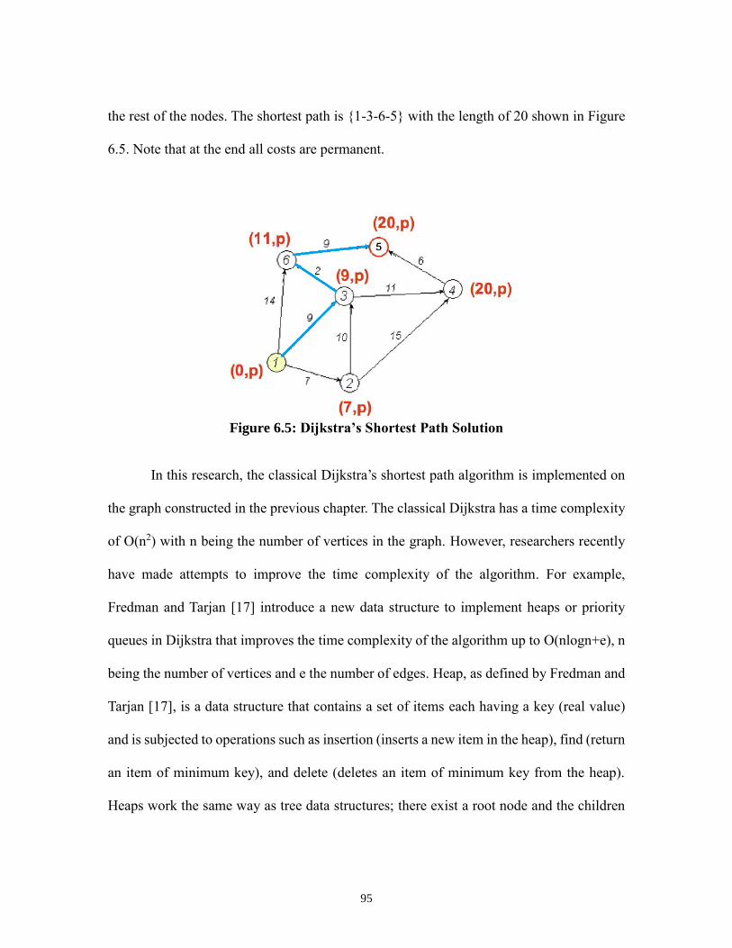
95

the rest of the nodes. The shortest path is {1-3-6-5} with the length of 20 shown in Figure

6.5. Note that at the end all costs are permanent.

Figure 6.5: Dijkstra’s Shortest Path Solution

In this research, the classical Dijkstra’s shortest path algorithm is implemented on

the graph constructed in the previous chapter. The classical Dijkstra has a time complexity

of O(n2) with n being the number of vertices in the graph. However, researchers recently

have made attempts to improve the time complexity of the algorithm. For example,

Fredman and Tarjan [17] introduce a new data structure to implement heaps or priority

queues in Dijkstra that improves the time complexity of the algorithm up to O(nlogn+e), n

being the number of vertices and e the number of edges. Heap, as defined by Fredman and

Tarjan [17], is a data structure that contains a set of items each having a key (real value)

and is subjected to operations such as insertion (inserts a new item in the heap), find (return

an item of minimum key), and delete (deletes an item of minimum key from the heap).

Heaps work the same way as tree data structures; there exist a root node and the children

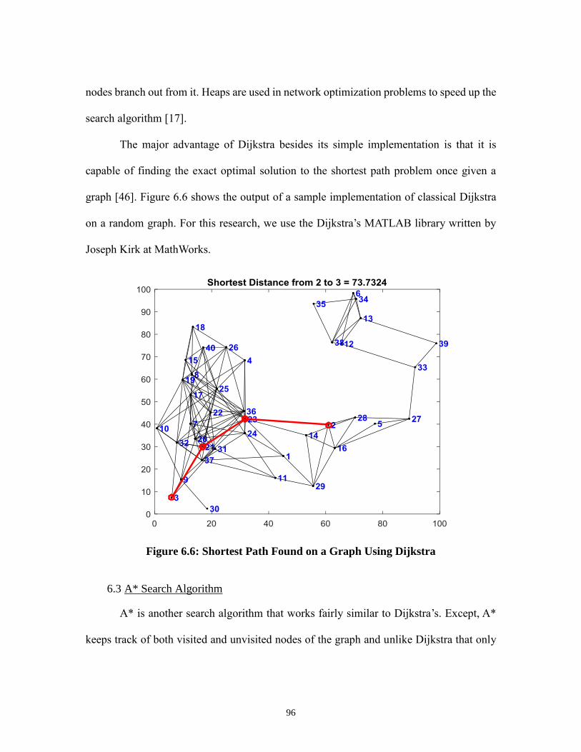
96

nodes branch out from it. Heaps are used in network optimization problems to speed up the

search algorithm [17].

The major advantage of Dijkstra besides its simple implementation is that it is

capable of finding the exact optimal solution to the shortest path problem once given a

graph [46]. Figure 6.6 shows the output of a sample implementation of classical Dijkstra

on a random graph. For this research, we use the Dijkstra’s MATLAB library written by

Joseph Kirk at MathWorks.

Figure 6.6: Shortest Path Found on a Graph Using Dijkstra

6.3 A* Search Algorithm

A* is another search algorithm that works fairly similar to Dijkstra’s. Except, A*

keeps track of both visited and unvisited nodes of the graph and unlike Dijkstra that only

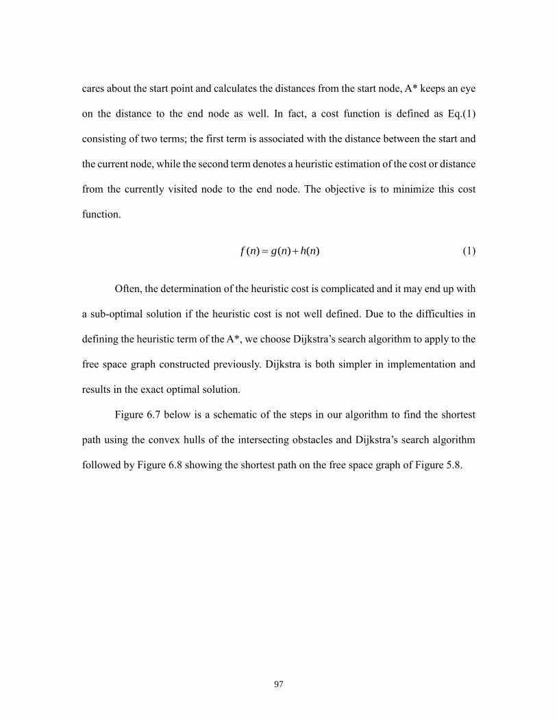
97

cares about the start point and calculates the distances from the start node, A* keeps an eye

on the distance to the end node as well. In fact, a cost function is defined as Eq.(1)

consisting of two terms; the first term is associated with the distance between the start and

the current node, while the second term denotes a heuristic estimation of the cost or distance

from the currently visited node to the end node. The objective is to minimize this cost

function.

( ) ( ) ( )f n g n h n (1)

Often, the determination of the heuristic cost is complicated and it may end up with

a sub-optimal solution if the heuristic cost is not well defined. Due to the difficulties in

defining the heuristic term of the A*, we choose Dijkstra’s search algorithm to apply to the

free space graph constructed previously. Dijkstra is both simpler in implementation and

results in the exact optimal solution.

Figure 6.7 below is a schematic of the steps in our algorithm to find the shortest

path using the convex hulls of the intersecting obstacles and Dijkstra’s search algorithm

followed by Figure 6.8 showing the shortest path on the free space graph of Figure 5.8.

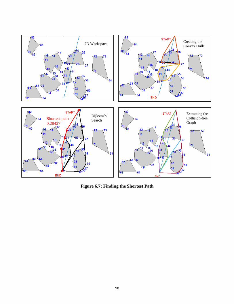
98

Figure 6.7: Finding the Shortest Path

2D Workspace Creating the

Convex Hulls

Extracting the

Collision-free

Graph

Dijkstra’s

Search Shortest path =

0.28427

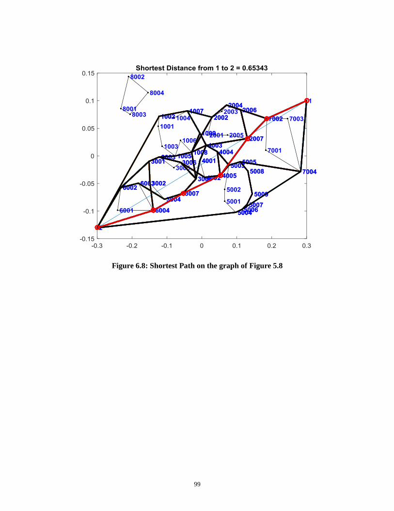
99

Figure 6.8: Shortest Path on the graph of Figure 5.8

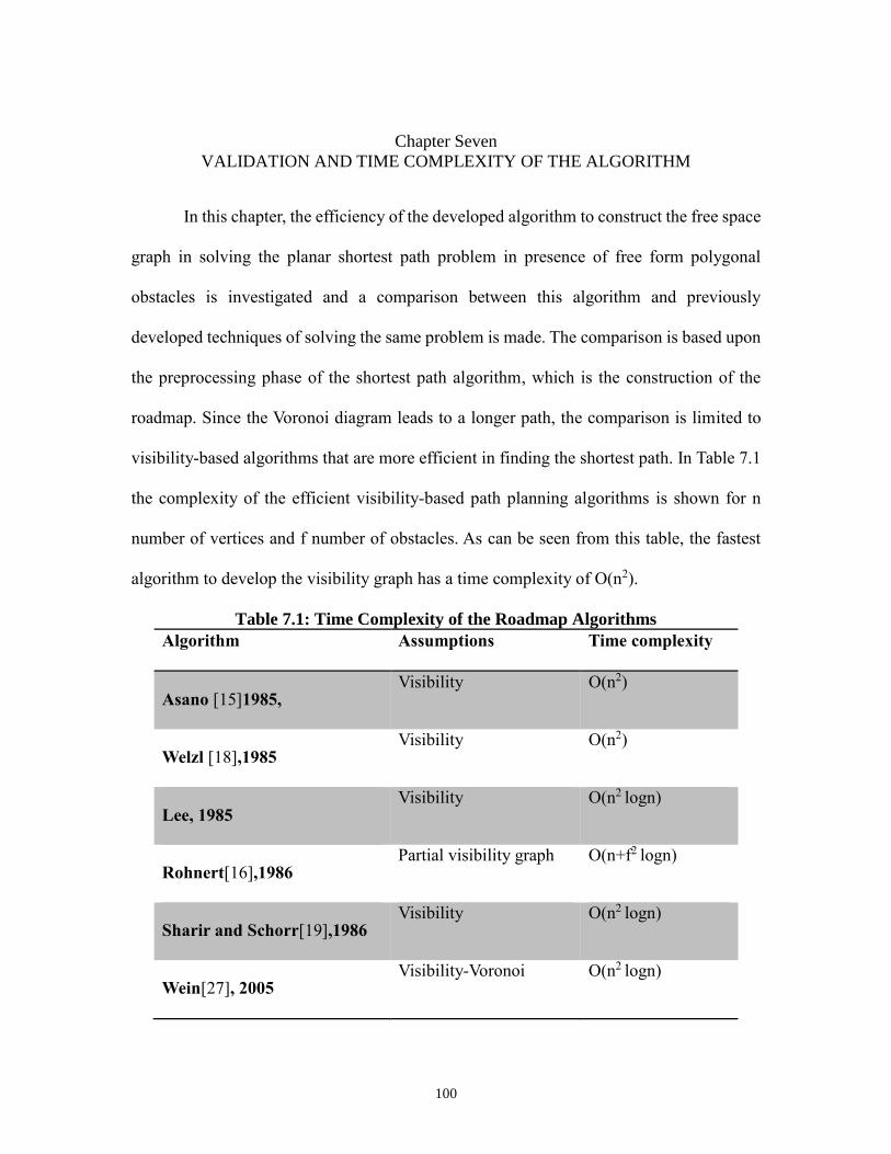
100

Chapter Seven

VALIDATION AND TIME COMPLEXITY OF THE ALGORITHM

In this chapter, the efficiency of the developed algorithm to construct the free space

graph in solving the planar shortest path problem in presence of free form polygonal

obstacles is investigated and a comparison between this algorithm and previously

developed techniques of solving the same problem is made. The comparison is based upon

the preprocessing phase of the shortest path algorithm, which is the construction of the

roadmap. Since the Voronoi diagram leads to a longer path, the comparison is limited to

visibility-based algorithms that are more efficient in finding the shortest path. In Table 7.1

the complexity of the efficient visibility-based path planning algorithms is shown for n

number of vertices and f number of obstacles. As can be seen from this table, the fastest

algorithm to develop the visibility graph has a time complexity of O(n2).

Table 7.1: Time Complexity of the Roadmap Algorithms

Algorithm Assumptions Time complexity

Asano [15]1985, Visibility O(n2)

Welzl [18],1985 Visibility O(n2)

Lee, 1985 Visibility O(n2 logn)

Rohnert[16],1986 Partial visibility graph O(n+f2 logn)

Sharir and Schorr[19],1986 Visibility O(n2 logn)

Wein[27], 2005 Visibility-Voronoi O(n2 logn)

101

In the following section, the complexity of the algorithm developed in this research

to come up with the free space graph is derived. Since the construction of the free space

graph is a preliminary basis for the path planning and provides the means for the

optimization/search algorithm, we call this phase of the path planning the preprocessing

phase. By this definition, the post-processing is allocated to the implementation of the

shortest path algorithm to search for the optimal (often times shortest) route.

7.1 Time Complexity of the C-Hull Based Roadmap

To determine the time complexity of the graph generation technique, we need to

first find the complexity of creating the convex hulls (C-hull). Because the complexity of

determining the line segment intersection is polynomial, O(n) (because one line segment

is checked with all n line segments of all obstacles, in the worst case), the dominant

algorithm in determining the complexity of the preprocessing phase is the generation of

the convex hulls. Hence, it suffices to determine the complexity of the C-hull generation.

The C-hull formation algorithm used in this research is known as Graham’s C-hull

technique and has a time complexity of O(nlogn) for n vertices, as mentioned in the

literature [14]. Hence, in the worst case, if all the f obstacles of the workspace are

intersecting the route, the complexity of forming the C-hulls will be O(nlog(n/f)) with n

being the total number of vertices. This complexity is the complexity of the graph

construction in the worst case since graph construction is nothing but generating the C-

hulls. As for f obstacles, 4f C-hulls are generated (as explained in chapter 5), assuming the

maximum number of vertices in each obstacle is nmax, the algorithm computes the total 4f

number of C-hulls in O(4f(nmax)log(nmax)) time in the worst case, using Graham’s

102

technique. Since the total number of vertices is designated by n, n is equal to f* nmax by this

notation, hence yielding the time complexity of O(nlog(n/f)) for the preprocessing.

The post-processing phase of the algorithm is to find the shortest path on the graph

constructed in the preprocessing. The Dijkstra algorithm used in this research is a classical

Dijkstra that has a complexity of O(n2) although using the heap based Dijkstra or A*

algorithm would result in a faster search-for-the-shortest-paths process.

A comparison of the preprocessing complexity of the algorithm developed in this

research and the previous methods show an improvement in the time complexity of the

preprocessing of the planar shortest path due to restricting the construction of the free space

graph to a portion of the plane rather than generating the graph of the entire workspace.

This results in a smaller graph, thus, simplifies and speeds up the search for the shortest

path on this smaller graph.

7.2 Validation

This algorithm is tested on different planar workspaces with a variety of obstacles

from one to 50 obstacles. The obstacles can have any arbitrary shapes thanks to the

tessellated geometric representation of the workspace that is capable of handling any free

form surfaces and solid models. The results are shown in Appendix A. The tests have been

made based upon the number of obstacles, total number of vertices, average number of

vertices per obstacle, number of reflex vertices, and the density of the workspace

determined by the clearance between the obstacles. In all cases, the algorithm is able to

find the shortest path, though an increase in the number of intersecting obstacles and/or the

average vertices per obstacle, and density of the workspace obviously slows down the

103

computation by adding complexities to the problem. The complexity of the algorithm does

not depend on the number of obstacles in the workspace, in general, despite its dependence

on the number of intersecting obstacles. Also, the number of reflex vertices does not affect

the computational time since the C-hulls do not include any reflex vertex and in the

construction of the C-hulls, all vertices are treated the same way no matter they are convex

or reflex.

This algorithm is simple and robust since the C-hulls can be generated repeatedly

and recursively for any types and sizes of the workspace.

104

Chapter Eight

CONCLUSIONS AND FUTURE WORK

In this research, the problem of constructing a collision free graph (free space

graph) of a cluttered 2D environment and planning the shortest path between any arbitrary

pairs of nodes in that graph has been studied and the results are presented. The developed

algorithm could be applied to any planar environments with scattered free form (both

convex and concave) obstacles. Since the obstacles are tessellated in a CAD software, they

can have any shapes and their shapes can be simply processed through the program.

The preliminaries of the algorithm consist of reading the tessellated geometries in

a VRML format and storing the data of the coordinates of the vertices and connectivities

(edges that connect two vertices of an obstacle). The preprocessing of the algorithm is

about constructing the free space graph based upon the result of the line segment

intersection check and formation of the C-hulls of the intersecting obstacles (detected using

the bi-level collision detector). The preprocessing algorithm is proved to have a time

complexity of order O(nlog(n/f)) with n being the total number of vertices in the workspace

and f the number of obstacles directly in the path. Instead of studying the entire workspace,

we restrict the graph construction and search to a portion of it including the reference line

and the interfering obstacles. The post-processing of the algorithm is allocated to finding

the shortest path on the graph between the two specified nodes using the classical Dijkstra’s

shortest path algorithm in O(n2) time. Further improvements can be made to the algorithm

through the implementation of a more efficient search algorithm such as heap-based

105

Dijkstra or A*. The classical Dijkstra is used in this research for its simplicity of

implementation, which is slightly compromised by its speed of computation.

This algorithm is capable of finding the shortest path between two nodes on any

planar workspace with any number of free form obstacles and vertices. We claim that the

developed algorithm could be applied to 3D spatial workspaces as well though with a

greater time complexity. This will be further investigated in a separate research work.

Despite the improvements in the efficiency of the developed algorithm by focusing

on a portion of the workspace limited by the reference line and the intersecting obstacles,

it highly depends on the start and end points of the path. Hence, changing the start and end

points of the path results in a different free space graph while the visibility graph constructs

a single constant roadmap of the entire workspace. Having the roadmap of the entire

workspace has an advantage of being able to route the shortest path between any two nodes

of the graph. However, in the C-hull based path planning, if the shortest path between

different pairs of nodes is desired, the corresponding free space graph must be calculated

one at a time and the resultant graph would be the union of these subgraphs. For example,

consider the planar workspace shown in Figure 8.1. If the shortest path between both pairs

of nodes (61, 73) and (82, 53) are required, the algorithm first constructs the free space

graph between the two nodes 61 and 73 (Shown in Figure 8.2) and then 82 and 53 (Figure

8.3). Then, the edges of the free space graph for the pair of (82, 53) not included in the

graph of (61, 73) are added to the latter graph and the shortest path between the two nodes

can be found using single source Dijkstra’s algorithm. The resultant union of the two graphs

is shown in Figure 8.4.

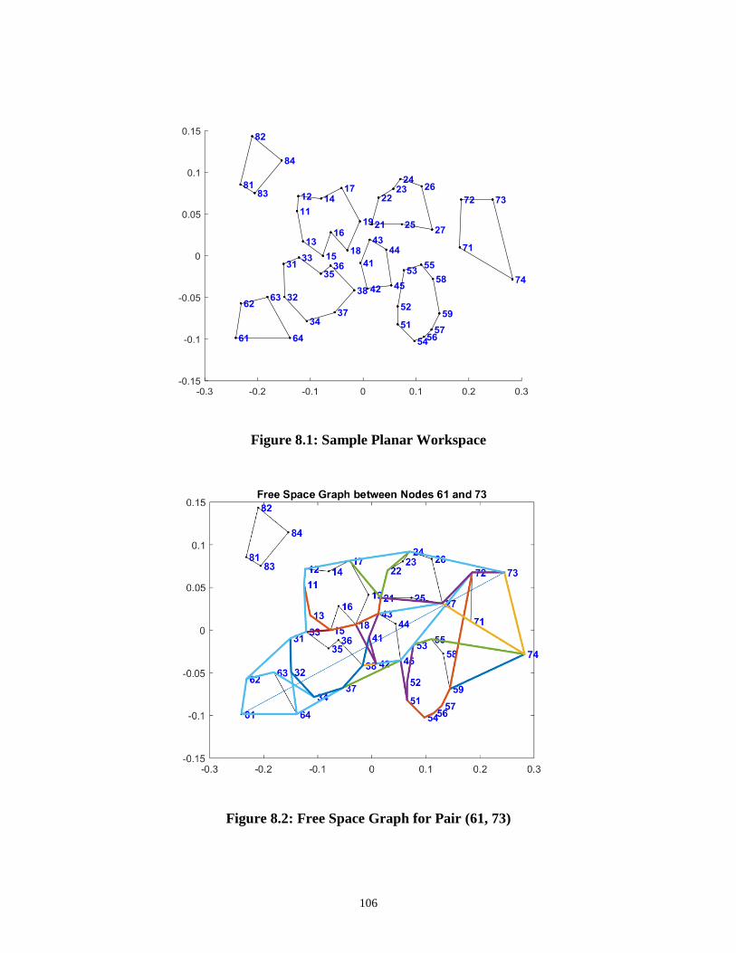
106

Figure 8.1: Sample Planar Workspace

Figure 8.2: Free Space Graph for Pair (61, 73)

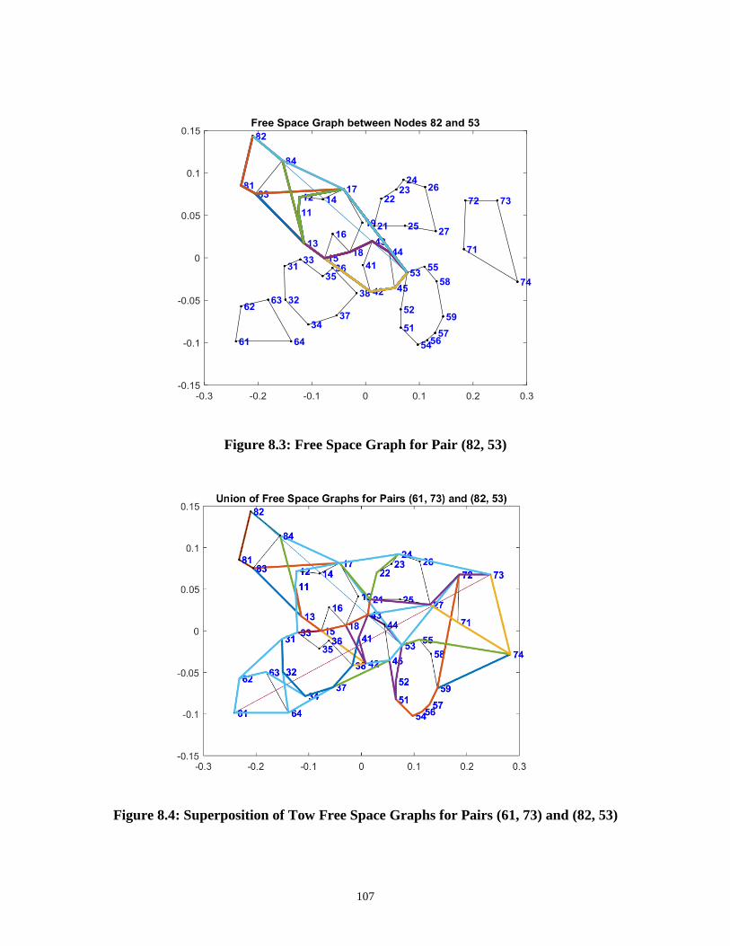
107

Figure 8.3: Free Space Graph for Pair (82, 53)

Figure 8.4: Superposition of Tow Free Space Graphs for Pairs (61, 73) and (82, 53)

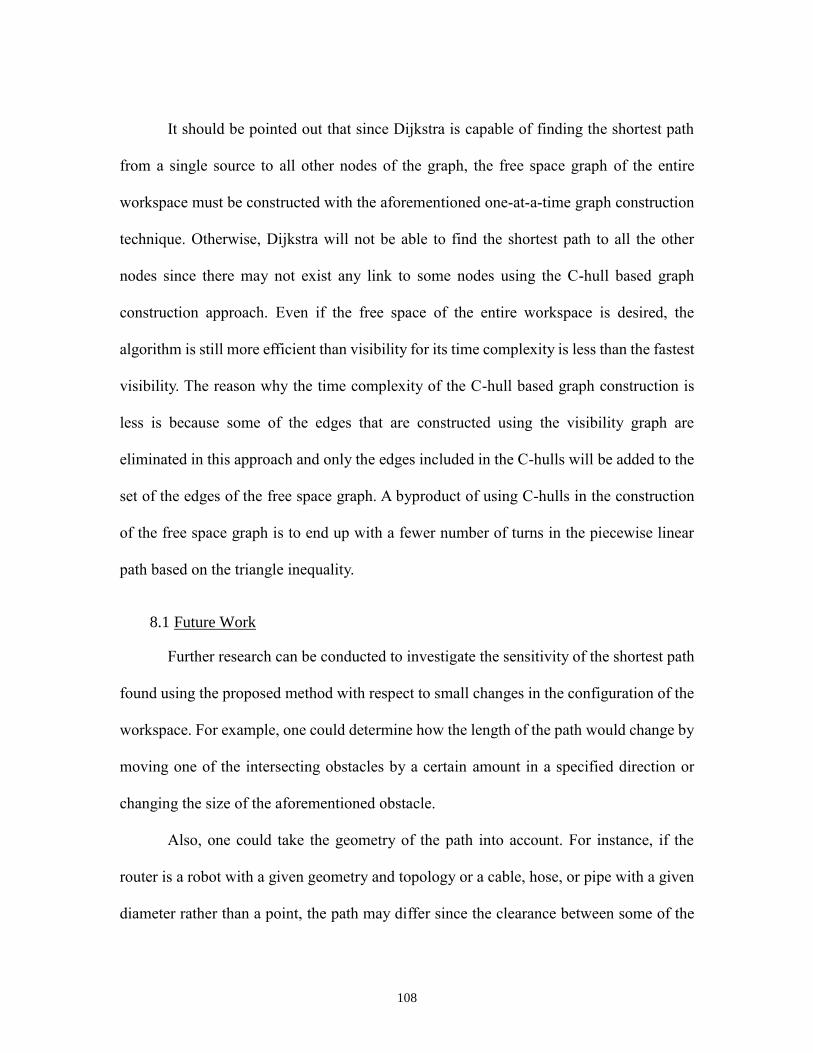
108

It should be pointed out that since Dijkstra is capable of finding the shortest path

from a single source to all other nodes of the graph, the free space graph of the entire

workspace must be constructed with the aforementioned one-at-a-time graph construction

technique. Otherwise, Dijkstra will not be able to find the shortest path to all the other

nodes since there may not exist any link to some nodes using the C-hull based graph

construction approach. Even if the free space of the entire workspace is desired, the

algorithm is still more efficient than visibility for its time complexity is less than the fastest

visibility. The reason why the time complexity of the C-hull based graph construction is

less is because some of the edges that are constructed using the visibility graph are

eliminated in this approach and only the edges included in the C-hulls will be added to the

set of the edges of the free space graph. A byproduct of using C-hulls in the construction

of the free space graph is to end up with a fewer number of turns in the piecewise linear

path based on the triangle inequality.

8.1 Future Work

Further research can be conducted to investigate the sensitivity of the shortest path

found using the proposed method with respect to small changes in the configuration of the

workspace. For example, one could determine how the length of the path would change by

moving one of the intersecting obstacles by a certain amount in a specified direction or

changing the size of the aforementioned obstacle.

Also, one could take the geometry of the path into account. For instance, if the

router is a robot with a given geometry and topology or a cable, hose, or pipe with a given

diameter rather than a point, the path may differ since the clearance between some of the

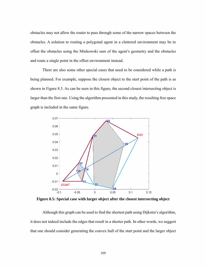
109

obstacles may not allow the router to pass through some of the narrow spaces between the

obstacles. A solution to routing a polygonal agent in a cluttered environment may be to

offset the obstacles using the Minkowski sum of the agent’s geometry and the obstacles

and route a single point in the offset environment instead.

There are also some other special cases that need to be considered while a path is

being planned. For example, suppose the closest object to the start point of the path is as

shown in Figure 8.5. As can be seen in this figure, the second closest intersecting object is

larger than the first one. Using the algorithm presented in this study, the resulting free space

graph is included in the same figure.

Figure 8.5: Special case with larger object after the closest intersecting object

Although this graph can be used to find the shortest path using Dijkstra’s algorithm,

it does not indeed include the edges that result in a shorter path. In other words, we suggest

that one should consider generating the convex hull of the start point and the larger object

110

rather than the smaller though closer object. This is because the convex hull with the larger

object also includes the entire (or parts of the) smaller intersecting object; hence,

overcoming the problem of interfering with this object. The free space graph using the

convex hull of the larger intersecting object is created for this example and shown in Figure

8.6. In addition, based on the triangle inequality, this convex hull will result in shorter paths

from the start to the end point. For example, in Figure 8.6 an edge from the start point of

the path to node 21 is created which is shorter than the sum of Start-12 and 12-21 edges

based on the triangle inequality.

After the free space graph is generated the Dijkstra’s algorithm is implemented to

find the shortest path on it from the start node to the end node. The results of Dijkstra on

both graphs is compared in Figure 8.7. As can be seen from this figure, the graph generated

using the convex hull of the larger object yields a shorter path.

Figure 8.6: Free space graph using the convex hull of the larger intersecting object

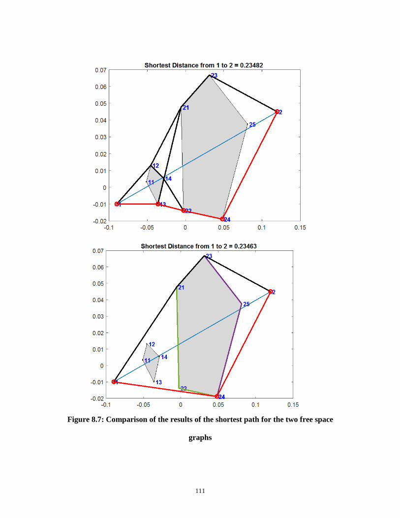
111

Figure 8.7: Comparison of the results of the shortest path for the two free space

graphs

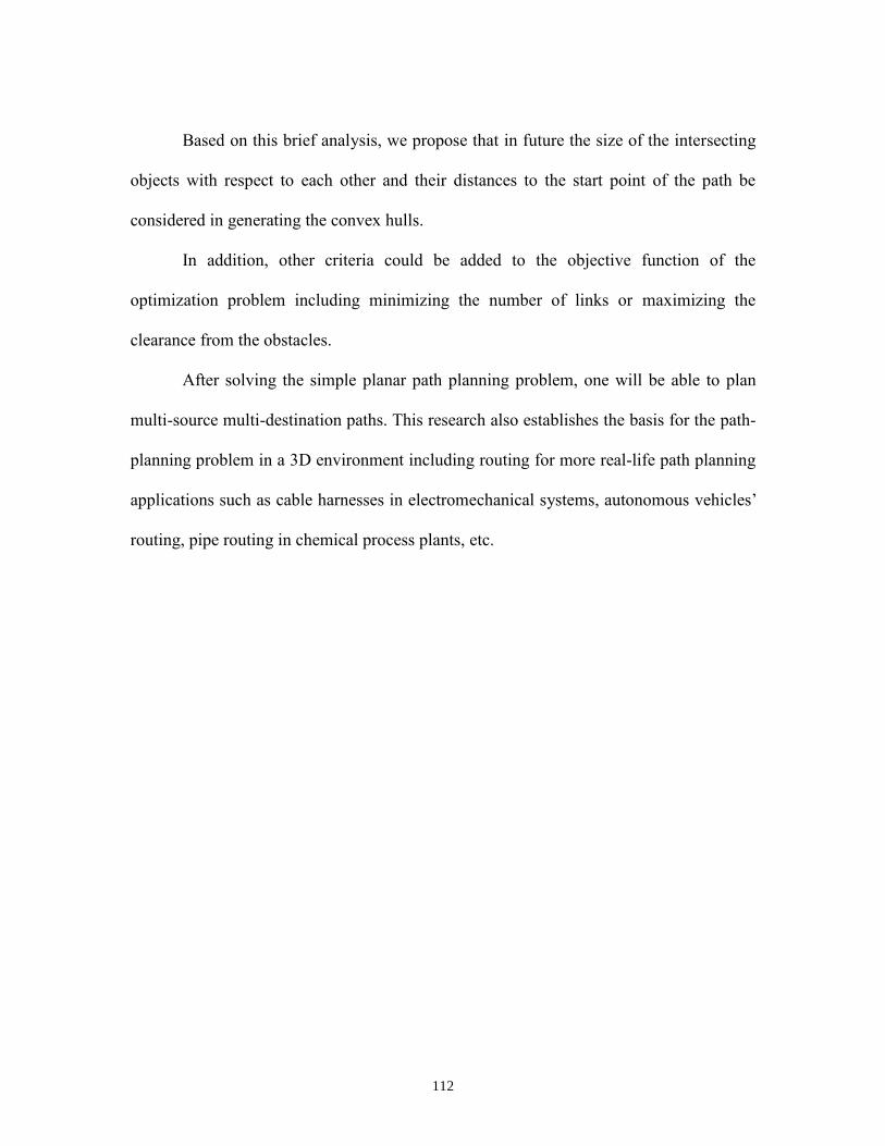
112

Based on this brief analysis, we propose that in future the size of the intersecting

objects with respect to each other and their distances to the start point of the path be

considered in generating the convex hulls.

In addition, other criteria could be added to the objective function of the

optimization problem including minimizing the number of links or maximizing the

clearance from the obstacles.

After solving the simple planar path planning problem, one will be able to plan

multi-source multi-destination paths. This research also establishes the basis for the path-

planning problem in a 3D environment including routing for more real-life path planning

applications such as cable harnesses in electromechanical systems, autonomous vehicles’

routing, pipe routing in chemical process plants, etc.

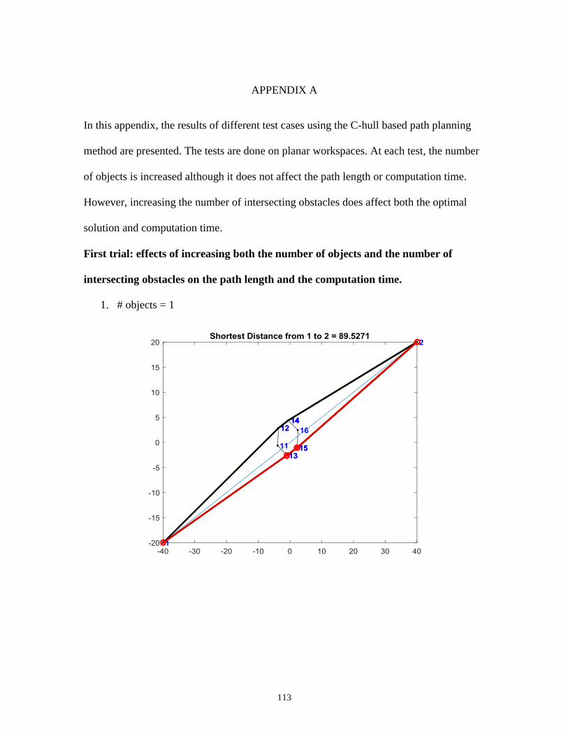
113

APPENDIX A

In this appendix, the results of different test cases using the C-hull based path planning

method are presented. The tests are done on planar workspaces. At each test, the number

of objects is increased although it does not affect the path length or computation time.

However, increasing the number of intersecting obstacles does affect both the optimal

solution and computation time.

First trial: effects of increasing both the number of objects and the number of

intersecting obstacles on the path length and the computation time.

1. # objects = 1

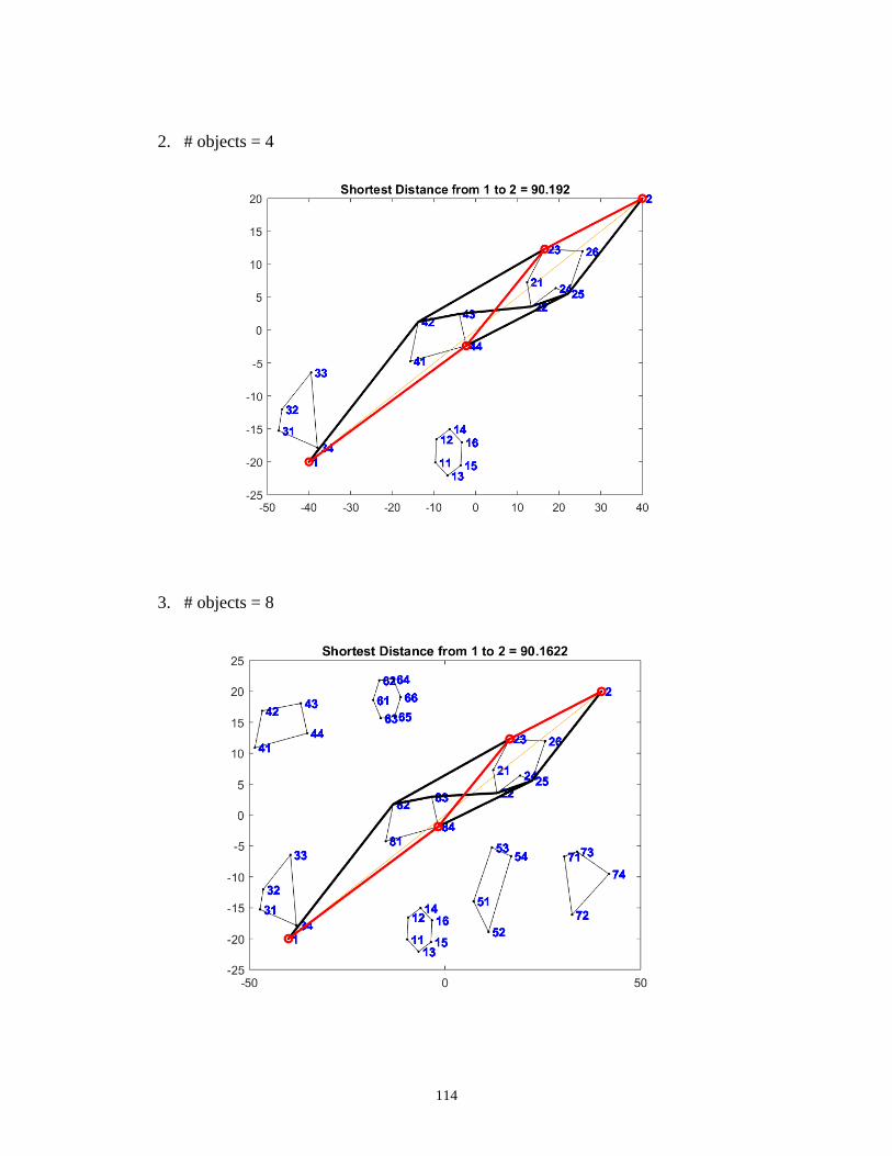
114

2. # objects = 4

3. # objects = 8

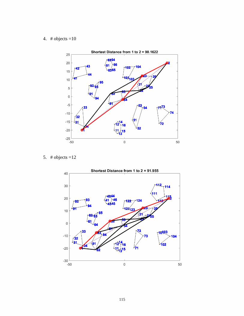
115

4. # objects =10

5. # objects =12

116

6. # objects =15

7. # objects =18

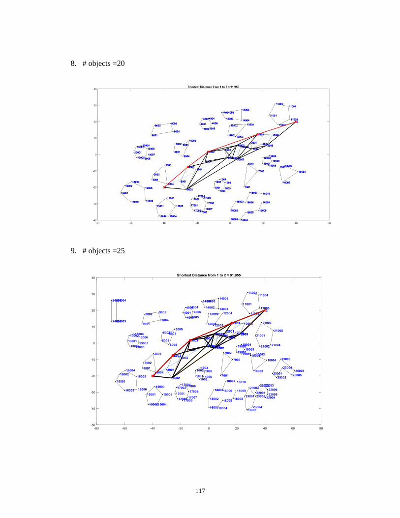
117

8. # objects =20

9. # objects =25

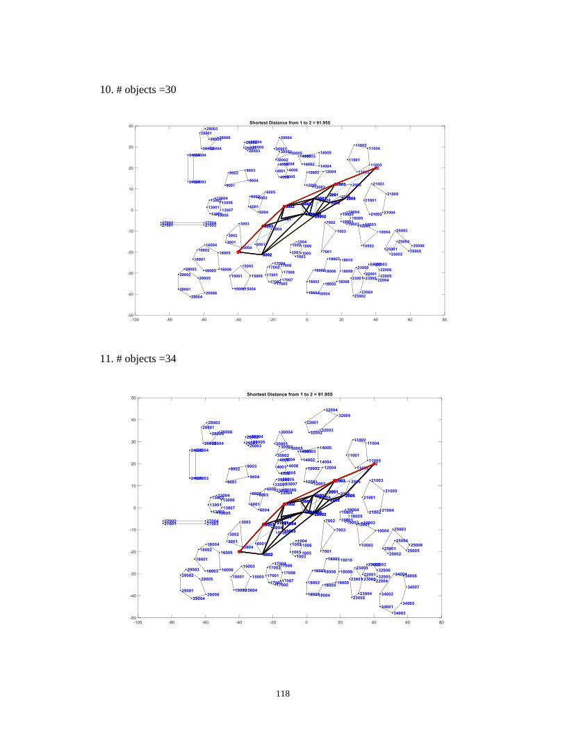
118

10. # objects =30

11. # objects =34

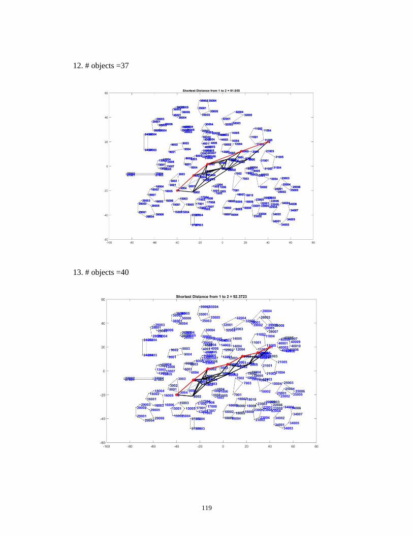
119

12. # objects =37

13. # objects =40

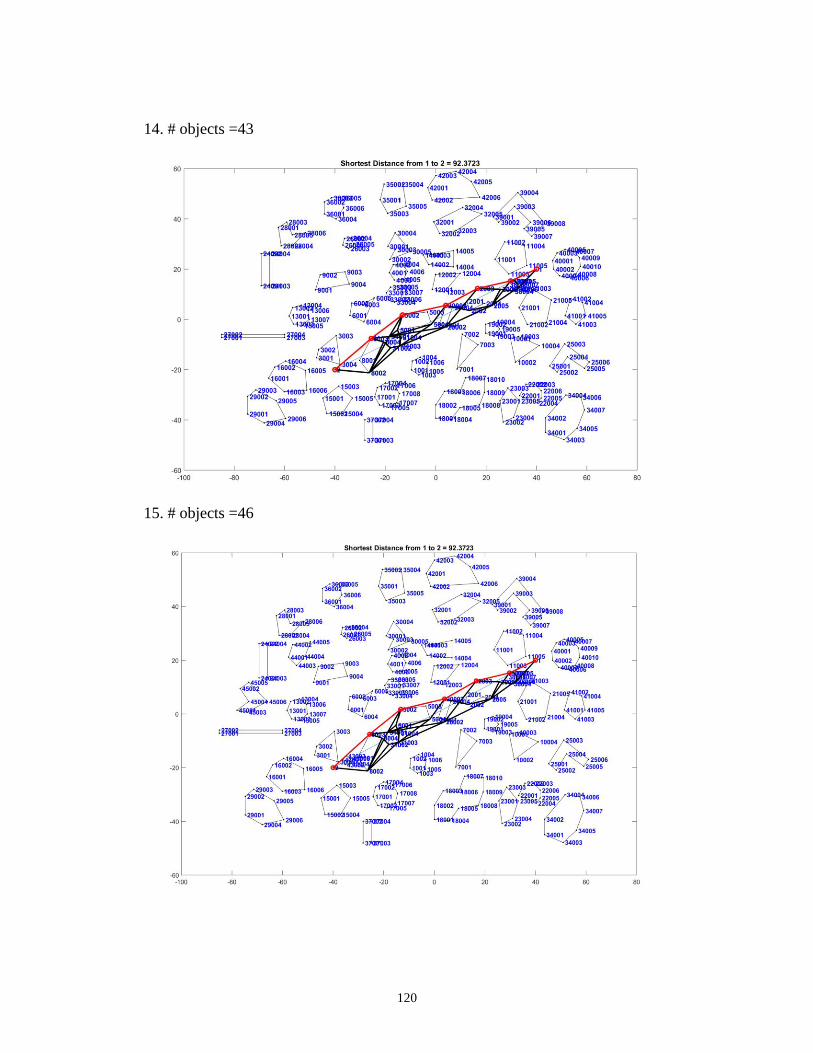
120

14. # objects =43

15. # objects =46

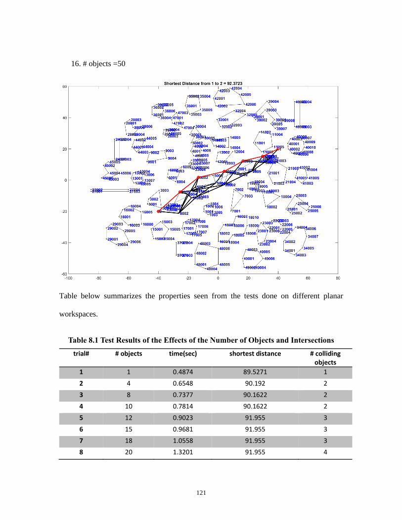
121

16. # objects =50

Table below summarizes the properties seen from the tests done on different planar

workspaces.

Table 8.1 Test Results of the Effects of the Number of Objects and Intersections

trial# # objects time(sec) shortest distance # colliding objects

1 1 0.4874 89.5271 1

2 4 0.6548 90.192 2

3 8 0.7377 90.1622 2

4 10 0.7814 90.1622 2

5 12 0.9023 91.955 3

6 15 0.9681 91.955 3

7 18 1.0558 91.955 3

8 20 1.3201 91.955 4

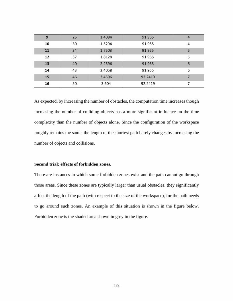
122

9 25 1.4084 91.955 4

10 30 1.5294 91.955 4

11 34 1.7503 91.955 5

12 37 1.8128 91.955 5

13 40 2.2596 91.955 6

14 43 2.4058 91.955 6

15 46 3.4596 92.2419 7

16 50 3.604 92.2419 7

As expected, by increasing the number of obstacles, the computation time increases though

increasing the number of colliding objects has a more significant influence on the time

complexity than the number of objects alone. Since the configuration of the workspace

roughly remains the same, the length of the shortest path barely changes by increasing the

number of objects and collisions.

Second trial: effects of forbidden zones.

There are instances in which some forbidden zones exist and the path cannot go through

those areas. Since these zones are typically larger than usual obstacles, they significantly

affect the length of the path (with respect to the size of the workspace), for the path needs

to go around such zones. An example of this situation is shown in the figure below.

Forbidden zone is the shaded area shown in grey in the figure.

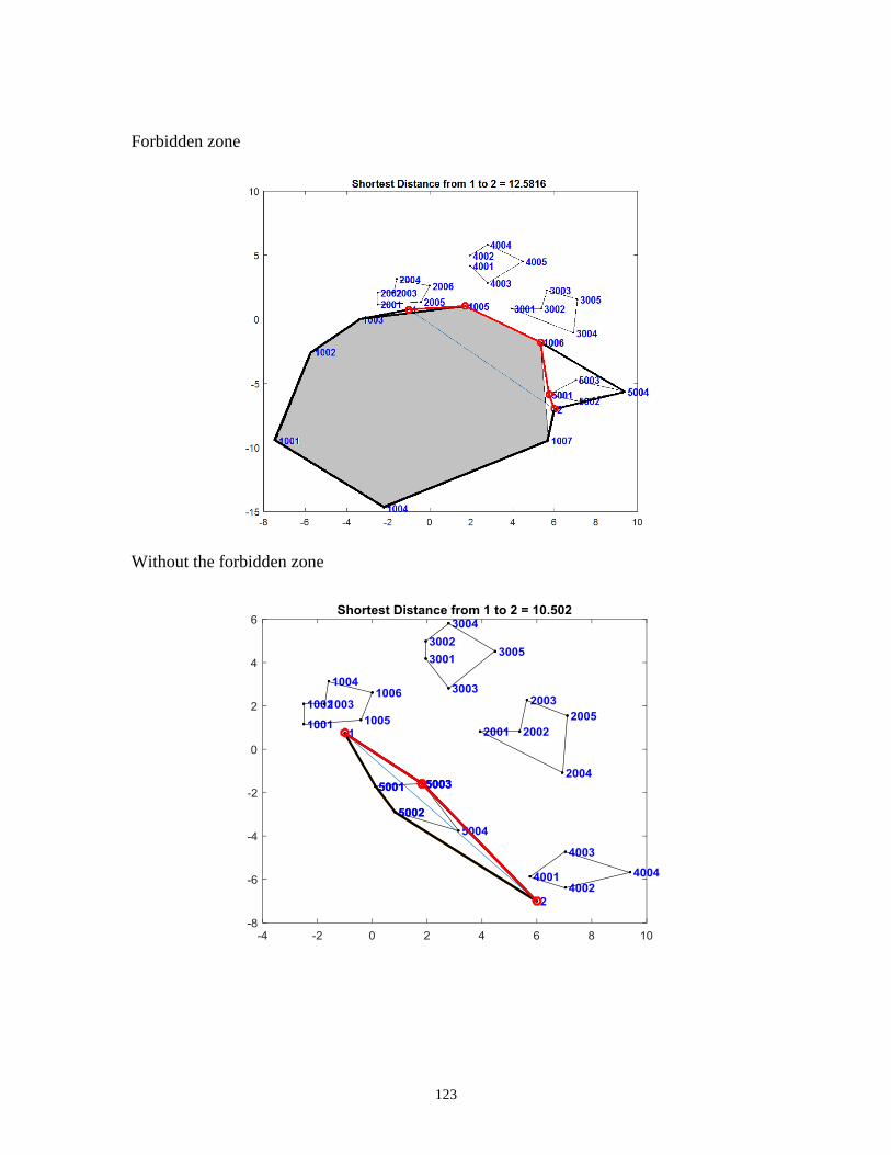
123

Forbidden zone

Without the forbidden zone

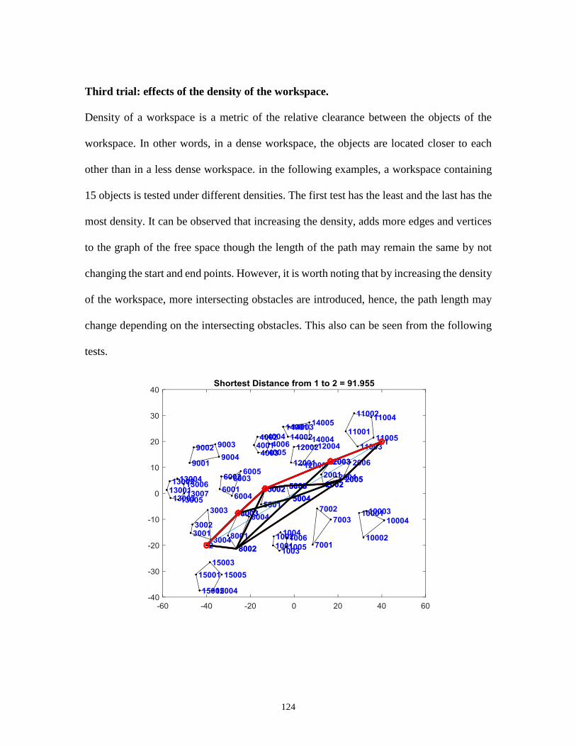
124

Third trial: effects of the density of the workspace.

Density of a workspace is a metric of the relative clearance between the objects of the

workspace. In other words, in a dense workspace, the objects are located closer to each

other than in a less dense workspace. in the following examples, a workspace containing

15 objects is tested under different densities. The first test has the least and the last has the

most density. It can be observed that increasing the density, adds more edges and vertices

to the graph of the free space though the length of the path may remain the same by not

changing the start and end points. However, it is worth noting that by increasing the density

of the workspace, more intersecting obstacles are introduced, hence, the path length may

change depending on the intersecting obstacles. This also can be seen from the following

tests.

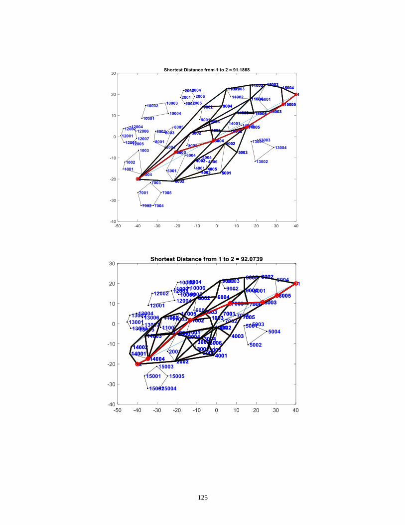
125

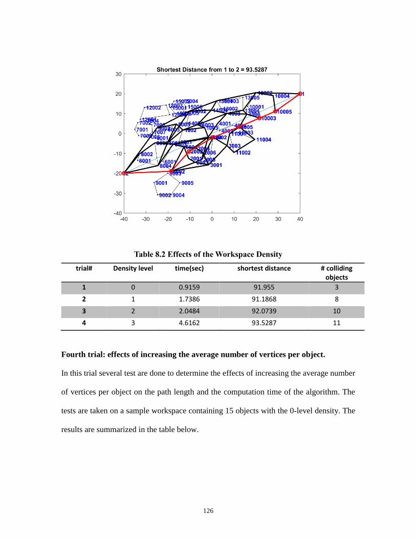
126

Table 8.2 Effects of the Workspace Density

trial# Density level time(sec) shortest distance # colliding objects

1 0 0.9159 91.955 3

2 1 1.7386 91.1868 8

3 2 2.0484 92.0739 10

4 3 4.6162 93.5287 11

Fourth trial: effects of increasing the average number of vertices per object.

In this trial several test are done to determine the effects of increasing the average number

of vertices per object on the path length and the computation time of the algorithm. The

tests are taken on a sample workspace containing 15 objects with the 0-level density. The

results are summarized in the table below.

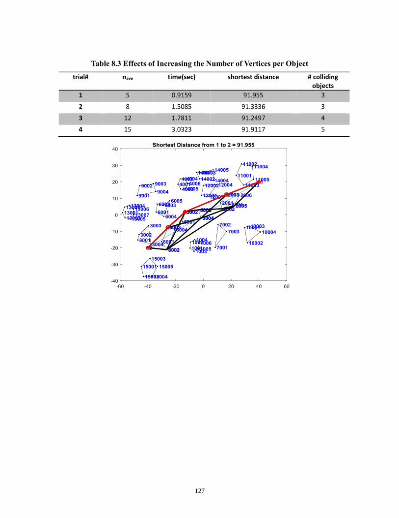
127

Table 8.3 Effects of Increasing the Number of Vertices per Object

trial# nave time(sec) shortest distance # colliding objects

1 5 0.9159 91.955 3

2 8 1.5085 91.3336 3

3 12 1.7811 91.2497 4

4 15 3.0323 91.9117 5

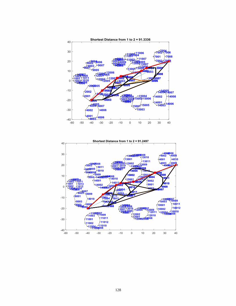
128

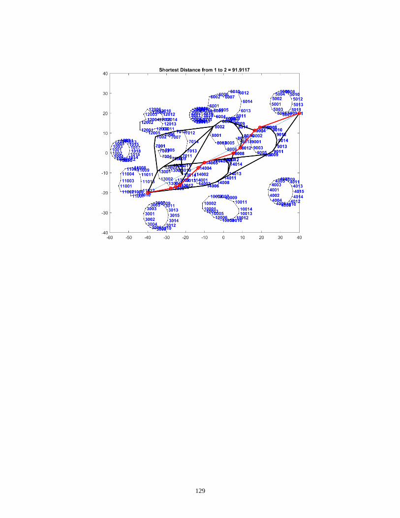
129

130

APPENDIX B

In this appendix, the MATLAB codes for analyzing and computing different parts of the

method are presented. The authors of the read_vrml, line-segment intersection and

Dijkstra’s libraries are included in the respective codes.

1. Reading the VRML data

%/*********************************************************

************************

% FUNCTION NAME : read_vrml

% AUTHOR : G. Akroyd

% PURPOSE : reads a VRML or Inventor file and stores data

points and connectivity

% in arrays ready for drawing wireframe images.

%

% VARIABLES/PARAMETERS:

% i/p filename name of vrml file

% o/p nel number of geometry parts (elements)

in file

% o/p w3d geometry structure ;-

% w3d.pts array of x y z values for

each element

% w3d.knx array of connection nodes

for each element

% w3d.color color of each element

% w3d.polynum number of polygons for

each element

% w3d.trans transparency of each

element

%

% Version / Date : 3.0 / 23-9-02

% removed triang optn & replaced face

array Nan padding

% with 1st value padding to correct

opengl display prob.

% Version / Date : 2.0 / 17-7-00

% changed output to a structure rather

than separate arrays

% to use less memory.

% 1.0 / 21-6-99

% original version

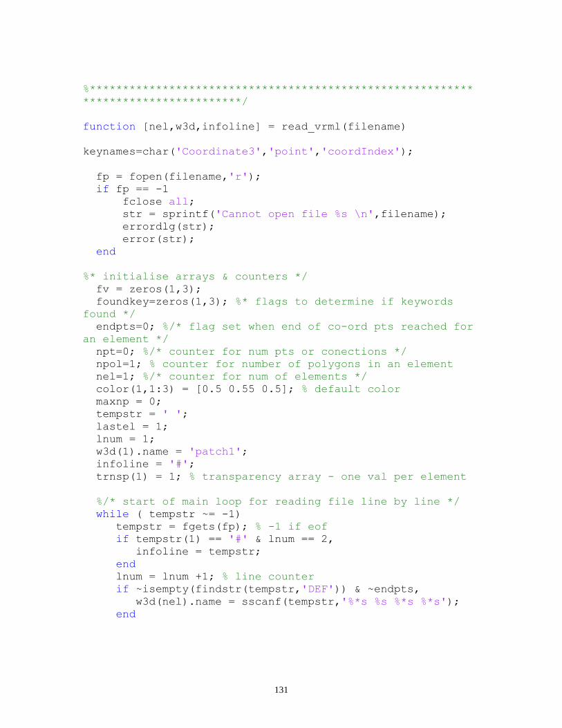
131

%**********************************************************

************************/

function [nel,w3d,infoline] = read_vrml(filename)

keynames=char('Coordinate3','point','coordIndex');

fp = fopen(filename,'r');

if fp == -1

fclose all;

str = sprintf('Cannot open file %s \n',filename);

errordlg(str);

error(str);

end

%* initialise arrays & counters */

fv = zeros(1,3);

foundkey=zeros(1,3); %* flags to determine if keywords

found */

endpts=0; %/* flag set when end of co-ord pts reached for

an element */

npt=0; %/* counter for num pts or conections */

npol=1; % counter for number of polygons in an element

nel=1; %/* counter for num of elements */

color(1,1:3) = [0.5 0.55 0.5]; % default color

maxnp = 0;

tempstr = ' ';

lastel = 1;

lnum = 1;

w3d(1).name = 'patch1';

infoline = '#';

trnsp(1) = 1; % transparency array - one val per element

%/* start of main loop for reading file line by line */

while ( tempstr ~= -1)

tempstr = fgets(fp); % -1 if eof

if tempstr(1) == '#' & lnum == 2,

infoline = tempstr;

end

lnum = lnum +1; % line counter

if ~isempty(findstr(tempstr,'DEF')) & ~endpts,

w3d(nel).name = sscanf(tempstr,'%*s %s %*s %*s');

end

132

if ~isempty(findstr(tempstr,'rgb')) |

~isempty(findstr(tempstr,'diffuseColor')) % get color data

sp = findstr(tempstr,'[');

if isempty(sp), sp = 12 +

findstr(tempstr,'diffuseColor'); end

nc = 0;

if ~isempty(sp)

sp = sp +1;

[cvals,nc]=sscanf(tempstr(sp:length(tempstr)),'%f %f %f,');

end

if nc >= 3

if nel > lastel+1

for m = lastel+1:nel-1

color(m,1:3) = color(1,1:3); % if color

not set then make equal to 1st

end

end

% if multi colors set then populate color

matrix, this is an inventor feature

for s = 1:fix(nc/3)

color(s+nel-1,1:3) = cvals(3*s-2:3*s)';

lastel = s+nel-1;

end

end

end

if ~isempty(findstr(tempstr,'transparency')), % get

transparency level

sp = findstr(tempstr,'trans');

[tvals,nc]=sscanf(tempstr(sp+12:length(tempstr)),'%f');

if nc > 0, trnsp(nel) = tvals(1); end

end

for i=1:3 %/* check for each keyword in line */

key = deblank(keynames(i,:));

if ~isempty(findstr(tempstr,key)) &

isempty(findstr(tempstr,'#'))

%/* if key found again before all found there is

a problem

% so reset flag for that key */

if ~foundkey(i), foundkey(i)=1;else

foundkey(i)=0; end

if(i>1 & ~foundkey(i-1)) foundkey(i)=0; end %/*

previous key must exist first ! */

133

end

end

if(foundkey(1) & foundkey(2)) %/* start of if A first

2 keys found */

if foundkey(3) %/* scan for connectivity data */

tempstr = [tempstr,' #']; %/* last word marker

for end of line */

skip = '';

%/* loop puts integer values in a line into

connection array */

word = ' ';

while(word(1) ~= '#')

format = sprintf('%s %%s#',skip);

[word,nw] = sscanf(tempstr,format);

skip = [skip,'%*s'];

[node,nred] = sscanf(word,'%d,');

if nred>0

for p = 1:nred

if node(p) ~= -1

npt = npt +1;

% increment node value as matlab

counts from 1, vrml 0

w3d(nel).knx(npol,npt) = node(p)+1;

else

if npt > maxnp(nel), maxnp(nel) =

npt; end

npt = 0;

npol = npol + 1;

end

end

end

end

if ~isempty(findstr(tempstr,']')) %/* End of

data block marker */

polynum(nel)=npol-1; %/* store num of

polygons in this element */

endpts=0; %/* reset flag ready for next

element search */

npt=0;

npol=1;

foundkey = zeros(1,4); %/* reset keyword

flags for next search */

nel = nel+1; %/* now looking for next

element so increment counter

134

maxnp(nel) = 0;

w3d(nel).name = sprintf('patch%d',nel); %

name next block

end

end %/* end of scan for connectivity */

%/* got 1st 2 keys but not 3rd and not end of co-

ords data */

if(foundkey(2) & ~foundkey(3) & ~endpts) %/* scan

for pts data */

sp = findstr(tempstr,'[');

if isempty(sp)

%/* points data in x y z columns */

[fv,nv]=sscanf(tempstr,'%f %f %f,');

else

%/* if block start marker [ in line - need

to skip over it to data

% hence pointer to marker incremented */

sp = sp +1;

[fv,nv]=sscanf(tempstr(sp:length(tempstr)),'%f %f %f,');

end

if(nv>0)

if mod(nv,3) ~= 0

fclose(fp);

error('Error reading 3d wire co-

ordinates: should be x y z, on each line');

end

nov = fix(nv/3);

for p = 1:nov

npt = npt+1;

w3d(nel).pts(npt,1:3)=fv(3*p-2:3*p);

end

end

if ~isempty(findstr(tempstr,']')) %/* end of

pts data block */

endpts=1; %/* flag to stop entry to pts scan

while reading connections */

npt=0;

end

end %/* end of scan for data pts */

end %/* end of if A */

end %/* end of main loop */

if nel == 0

135

fclose(fp);

error('Error reading 3d file: no data found');

end

nel = nel -1;

% if not same number of verticies in each polygon we need

to fill

% out rest of row in array with 1st value

nc = size(color);

ts = size(trnsp);

for i = 1:nel

facs = w3d(i).knx;

ind1 = find(facs==0); [rown,coln] =

ind2sub(size(facs),ind1);

facs(ind1) = facs(rown);

w3d(i).knx = facs;

if i > 1 & i > nc(1), color(i,1:3) = color(1,1:3); end %

extend color array to cover all elements

w3d(i).color = color(i,1:3);

w3d(i).polynum = polynum(i);

if i > ts(2) | trnsp(i)==0,

trnsp(i) = 1;

end % extend transparency array to cover all elements

w3d(i).trans = trnsp(i);

end

fclose(fp);

% END OF FUNCTION read_vrml

%==========================================================

===========================

2. Bi-level collision detector

function intersected = BilevelDetector(line,comp_data,nel)

%% This function checks if a line identified by its start

and end points has full intersection with any of the

objects in a 2D workspace

% objects are identified either through their vertices or

their edges

% the function's inputs are the workspace data; coordinates

of each

136

% object's vertices and vertices link data determining the

edges of each

% object, the total number of objects in the workspace, and

the line data

% It then outputs a logical argument, 0 if no or partial

intersection and 1

% if full intersection occurs.

% the first section of this code checks if the object's

data is within the

% limits of line by looking into the bounding box

coordinates of the object

%----------------------------------------------------------

----------------

intersected = [];

% Boundary Check

ColBB = zeros(nel,1);

for i = 1:nel

if collision(line,comp_data{i,1}(:,(2:4))) == 1

ColBB(i) = 1;

else

ColBB(i) = 0;

end

end

% Line segment intersection detection

InBound = find(ColBB);

if isempty(InBound)

intersected = [];

else

XY1 = [line(1,(1:2)) line(2,(1:2))];

for j = 1:size(InBound,1)

XY2 = zeros(size(comp_data{InBound(j),2},1),4);

for k = 1:size(comp_data{InBound(j),2},1)

array = comp_data{InBound(j),2}(k,:);

XY2(k,(1:2)) =

comp_data{InBound(j),1}(array(1),(2:3));

XY2(k,(3:4)) =

comp_data{InBound(j),1}(array(2),(2:3));

end

out = lineSegmentIntersect_v2(XY1,XY2);

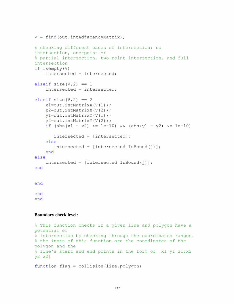
137

V = find(out.intAdjacencyMatrix);

% checking different cases of intersection: no

intersection, one-point or

% partial intersection, two-point intersection, and full

intersection

if isempty(V)

intersected = intersected;

elseif size(V,2) == 1

intersected = intersected;

elseif size(V,2) == 2

x1=out.intMatrixX(V(1));

x2=out.intMatrixX(V(2));

y1=out.intMatrixY(V(1));

y2=out.intMatrixY(V(2));

if (abs(x1 - x2) <= 1e-10) && (abs(y1 - y2) <= 1e-10)

intersected = [intersected];

else

intersected = [intersected InBound(j)];

end

else

intersected = [intersected InBound(j)];

end

end

end

end

Boundary check level:

% This function checks if a given line and polygon have a

potential of

% intersection by checking through the coordinates ranges.

% the inpts of this function are the coordinates of the

polygon and the

% line's start and end points in the form of [x1 y1 z1;x2

y2 z2]

function flag = collision(line,polygon)

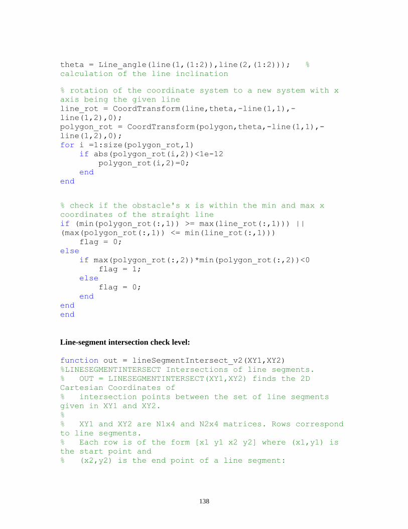
138

theta = Line_angle(line(1,(1:2)),line(2,(1:2))); %

calculation of the line inclination

% rotation of the coordinate system to a new system with x

axis being the given line

line_rot = CoordTransform(line,theta,-line(1,1),-

line(1,2),0);

polygon_rot = CoordTransform(polygon,theta,-line(1,1),-

line(1,2),0);

for i =1:size(polygon_rot,1)

if abs(polygon_rot(i,2))<1e-12

polygon_rot(i,2)=0;

end

end

% check if the obstacle's x is within the min and max x

coordinates of the straight line

if (min(polygon_rot(:,1)) >= max(line_rot(:,1))) ||

(max(polygon_rot(:,1)) <= min(line_rot(:,1)))

flag = 0;

else

if max(polygon_rot(:,2))*min(polygon_rot(:,2))<0

flag = 1;

else

flag = 0;

end

end

end

Line-segment intersection check level:

function out = lineSegmentIntersect_v2(XY1,XY2)

%LINESEGMENTINTERSECT Intersections of line segments.

% OUT = LINESEGMENTINTERSECT(XY1,XY2) finds the 2D

Cartesian Coordinates of

% intersection points between the set of line segments

given in XY1 and XY2.

%

% XY1 and XY2 are N1x4 and N2x4 matrices. Rows correspond

to line segments.

% Each row is of the form [x1 y1 x2 y2] where (x1,y1) is

the start point and

% (x2,y2) is the end point of a line segment:

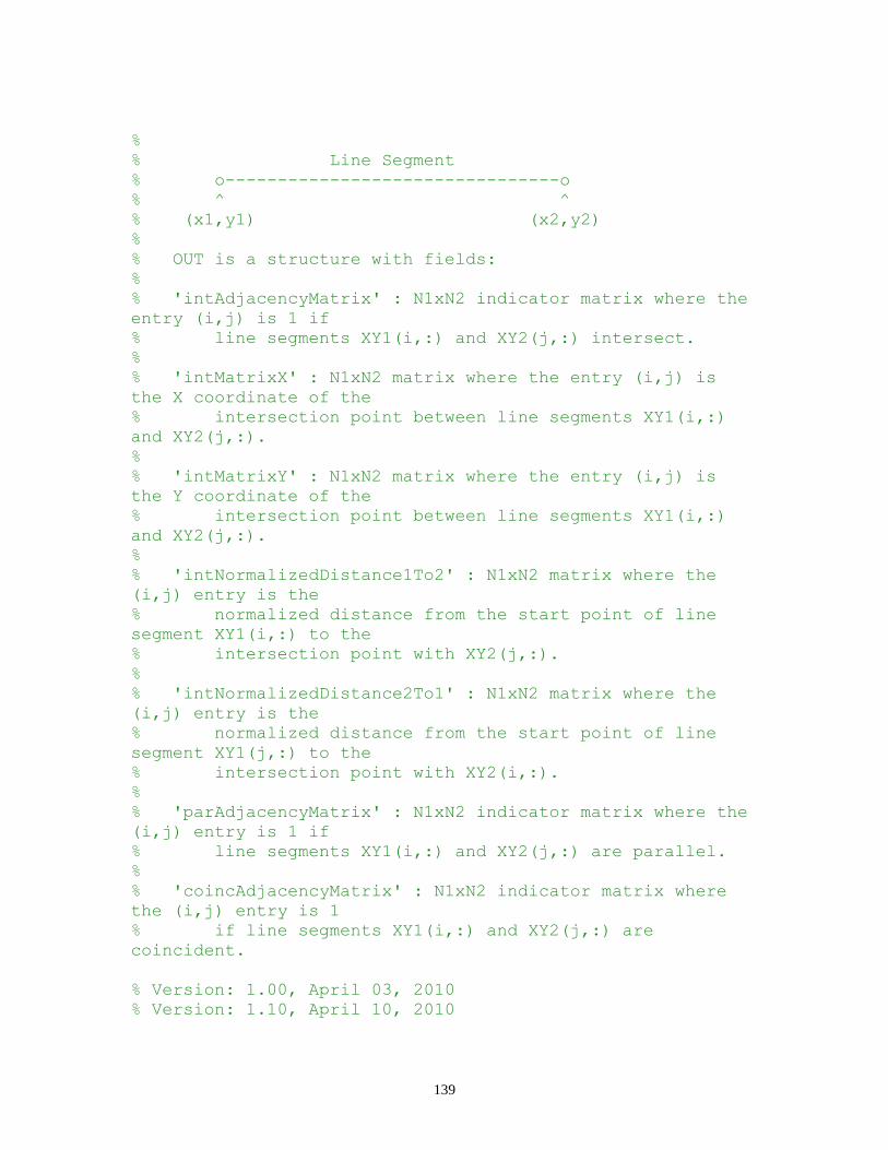
139

%

% Line Segment

% o--------------------------------o

% ^ ^

% (x1,y1) (x2,y2)

%

% OUT is a structure with fields:

%

% 'intAdjacencyMatrix' : N1xN2 indicator matrix where the

entry (i,j) is 1 if

% line segments XY1(i,:) and XY2(j,:) intersect.

%

% 'intMatrixX' : N1xN2 matrix where the entry (i,j) is

the X coordinate of the

% intersection point between line segments XY1(i,:)

and XY2(j,:).

%

% 'intMatrixY' : N1xN2 matrix where the entry (i,j) is

the Y coordinate of the

% intersection point between line segments XY1(i,:)

and XY2(j,:).

%

% 'intNormalizedDistance1To2' : N1xN2 matrix where the

(i,j) entry is the

% normalized distance from the start point of line

segment XY1(i,:) to the

% intersection point with XY2(j,:).

%

% 'intNormalizedDistance2To1' : N1xN2 matrix where the

(i,j) entry is the

% normalized distance from the start point of line

segment XY1(j,:) to the

% intersection point with XY2(i,:).

%

% 'parAdjacencyMatrix' : N1xN2 indicator matrix where the

(i,j) entry is 1 if

% line segments XY1(i,:) and XY2(j,:) are parallel.

%

% 'coincAdjacencyMatrix' : N1xN2 indicator matrix where

the (i,j) entry is 1

% if line segments XY1(i,:) and XY2(j,:) are

coincident.

% Version: 1.00, April 03, 2010

% Version: 1.10, April 10, 2010

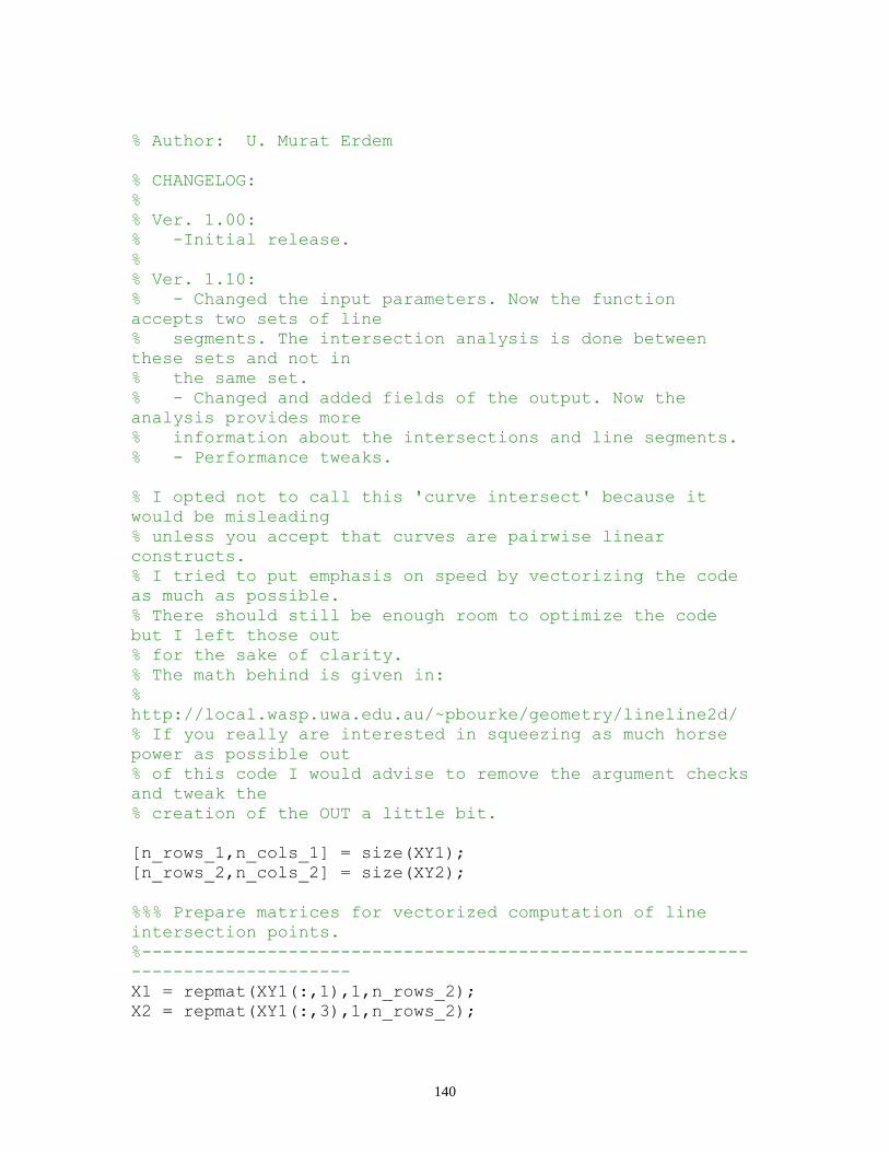
140

% Author: U. Murat Erdem

% CHANGELOG:

%

% Ver. 1.00:

% -Initial release.

%

% Ver. 1.10:

% - Changed the input parameters. Now the function

accepts two sets of line

% segments. The intersection analysis is done between

these sets and not in

% the same set.

% - Changed and added fields of the output. Now the

analysis provides more

% information about the intersections and line segments.

% - Performance tweaks.

% I opted not to call this 'curve intersect' because it

would be misleading

% unless you accept that curves are pairwise linear

constructs.

% I tried to put emphasis on speed by vectorizing the code

as much as possible.

% There should still be enough room to optimize the code

but I left those out

% for the sake of clarity.

% The math behind is given in:

%

http://local.wasp.uwa.edu.au/~pbourke/geometry/lineline2d/

% If you really are interested in squeezing as much horse

power as possible out

% of this code I would advise to remove the argument checks

and tweak the

% creation of the OUT a little bit.

[n_rows_1,n_cols_1] = size(XY1);

[n_rows_2,n_cols_2] = size(XY2);

%%% Prepare matrices for vectorized computation of line

intersection points.

%----------------------------------------------------------

---------------------

X1 = repmat(XY1(:,1),1,n_rows_2);

X2 = repmat(XY1(:,3),1,n_rows_2);

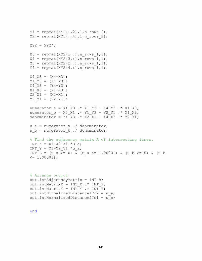
141

Y1 = repmat(XY1(:,2),1,n_rows_2);

Y2 = repmat(XY1(:,4),1,n_rows_2);

XY2 = XY2';

X3 = repmat(XY2(1,:),n_rows_1,1);

X4 = repmat(XY2(3,:),n_rows_1,1);

Y3 = repmat(XY2(2,:),n_rows_1,1);

Y4 = repmat(XY2(4,:),n_rows_1,1);

X4_X3 = (X4-X3);

Y1_Y3 = (Y1-Y3);

Y4_Y3 = (Y4-Y3);

X1_X3 = (X1-X3);

X2_X1 = (X2-X1);

Y2_Y1 = (Y2-Y1);

numerator_a = X4_X3 .* Y1_Y3 - Y4_Y3 .* X1_X3;

numerator_b = X2_X1 .* Y1_Y3 - Y2_Y1 .* X1_X3;

denominator = Y4_Y3 .* X2_X1 - X4_X3 .* Y2_Y1;

u_a = numerator_a ./ denominator;

u_b = numerator_b ./ denominator;

% Find the adjacency matrix A of intersecting lines.

INT_X = X1+X2_X1.*u_a;

INT_Y = Y1+Y2_Y1.*u_a;

INT_B = (u_a >= 0) & (u_a <= 1.00001) & (u_b >= 0) & (u_b

<= 1.00001);

% Arrange output.

out.intAdjacencyMatrix = INT_B;

out.intMatrixX = INT_X .* INT_B;

out.intMatrixY = INT_Y .* INT_B;

out.intNormalizedDistance1To2 = u_a;

out.intNormalizedDistance2To1 = u_b;

end

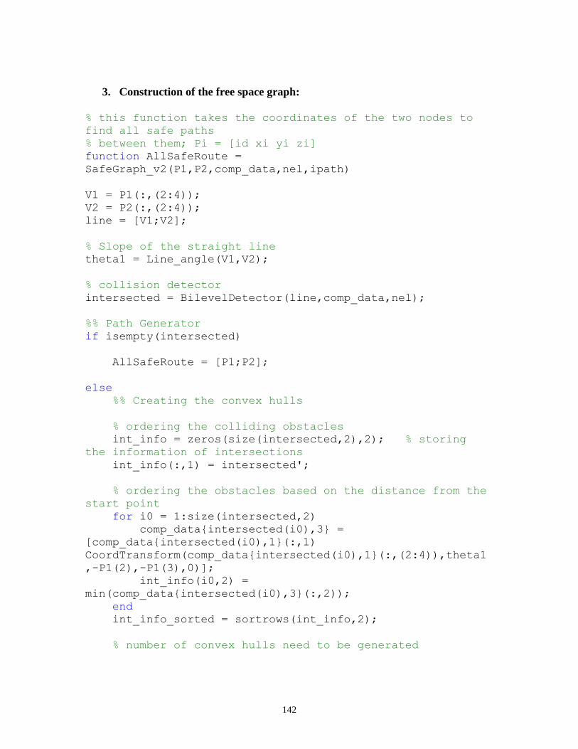
142

3. Construction of the free space graph:

% this function takes the coordinates of the two nodes to

find all safe paths

% between them; Pi = [id xi yi zi]

function AllSafeRoute =

SafeGraph_v2(P1,P2,comp_data,nel,ipath)

V1 = P1(:,(2:4));

V2 = P2(:,(2:4));

line = [V1;V2];

% Slope of the straight line

theta1 = Line_angle(V1,V2);

% collision detector

intersected = BilevelDetector(line,comp_data,nel);

%% Path Generator

if isempty(intersected)

AllSafeRoute = [P1;P2];

else

%% Creating the convex hulls

% ordering the colliding obstacles

int_info = zeros(size(intersected,2),2); % storing

the information of intersections

int_info(:,1) = intersected';

% ordering the obstacles based on the distance from the

start point

for i0 = 1:size(intersected,2)

comp_data{intersected(i0),3} =

[comp_data{intersected(i0),1}(:,1)

CoordTransform(comp_data{intersected(i0),1}(:,(2:4)),theta1

,-P1(2),-P1(3),0)];

int_info(i0,2) =

min(comp_data{intersected(i0),3}(:,2));

end

int_info_sorted = sortrows(int_info,2);

% number of convex hulls need to be generated

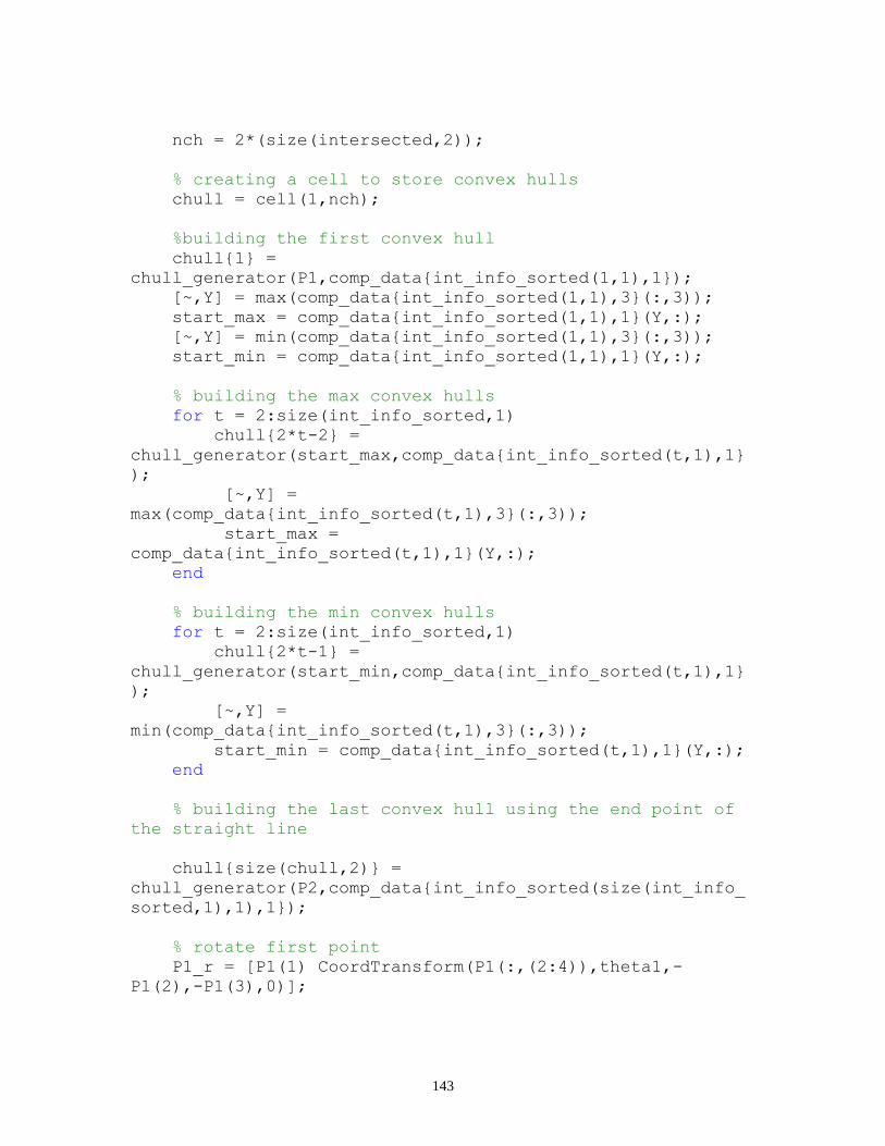
143

nch = 2*(size(intersected,2));

% creating a cell to store convex hulls

chull = cell(1,nch);

%building the first convex hull

chull{1} =

chull_generator(P1,comp_data{int_info_sorted(1,1),1});

[~,Y] = max(comp_data{int_info_sorted(1,1),3}(:,3));

start_max = comp_data{int_info_sorted(1,1),1}(Y,:);

[~,Y] = min(comp_data{int_info_sorted(1,1),3}(:,3));

start_min = comp_data{int_info_sorted(1,1),1}(Y,:);

% building the max convex hulls

for t = 2:size(int_info_sorted,1)

chull{2*t-2} =

chull_generator(start_max,comp_data{int_info_sorted(t,1),1}

);

[~,Y] =

max(comp_data{int_info_sorted(t,1),3}(:,3));

start_max =

comp_data{int_info_sorted(t,1),1}(Y,:);

end

% building the min convex hulls

for t = 2:size(int_info_sorted,1)

chull{2*t-1} =

chull_generator(start_min,comp_data{int_info_sorted(t,1),1}

);

[~,Y] =

min(comp_data{int_info_sorted(t,1),3}(:,3));

start_min = comp_data{int_info_sorted(t,1),1}(Y,:);

end

% building the last convex hull using the end point of

the straight line

chull{size(chull,2)} =

chull_generator(P2,comp_data{int_info_sorted(size(int_info_

sorted,1),1),1});

% rotate first point

P1_r = [P1(1) CoordTransform(P1(:,(2:4)),theta1,-

P1(2),-P1(3),0)];

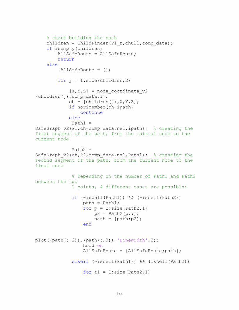
144

% start building the path

children = ChildFinder(P1_r,chull,comp_data);

if isempty(children)

AllSafeRoute = AllSafeRoute;

return

else

AllSafeRoute = {};

for j = 1:size(children,2)

[X,Y,Z] = node_coordinate_v2

(children(j),comp_data,1);

ch = [children(j),X,Y,Z];

if horimember(ch,ipath)

continue

else

Path1 =

SafeGraph_v2(P1,ch,comp_data,nel,ipath); % creating the

first segment of the path; from the initial node to the

current node

Path2 =

SafeGraph_v2(ch,P2,comp_data,nel,Path1); % creating the

second segment of the path; from the current node to the

final node

% Depending on the number of Path1 and Path2

between the two

% points, 4 different cases are possible:

if (~iscell(Path1)) && (~iscell(Path2))

path = Path1;

for p = 2:size(Path2,1)

p2 = Path2(p,:);

path = [path;p2];

end

plot((path(:,2)),(path(:,3)),'LineWidth',2);

hold on

AllSafeRoute = [AllSafeRoute;path];

elseif (~iscell(Path1)) && (iscell(Path2))

for t1 = 1:size(Path2,1)

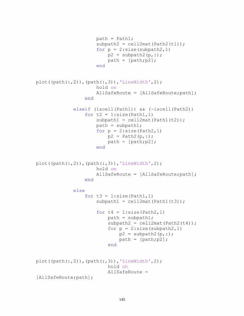
145

path = Path1;

subpath2 = cell2mat(Path2(t1));

for p = 2:size(subpath2,1)

p2 = subpath2(p,:);

path = [path;p2];

end


hold on


end

elseif (iscell(Path1)) && (~iscell(Path2))



path = subpath1;

for p = 2:size(Path2,1)

p2 = Path2(p,:);

path = [path;p2];

end


hold on


end

else




path = subpath1;


for p = 2:size(subpath2,1)

p2 = subpath2(p,:);

path = [path;p2];

end


hold on

AllSafeRoute =

[AllSafeRoute;path];

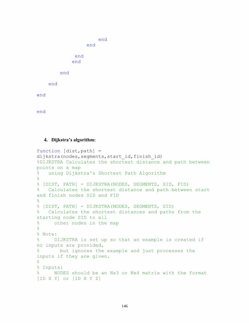
146

end

end

end

end

end

end

end

end

4. Dijkstra’s algorithm:

function [dist,path] =

dijkstra(nodes,segments,start_id,finish_id)

%DIJKSTRA Calculates the shortest distance and path between

points on a map

% using Dijkstra's Shortest Path Algorithm

%

% [DIST, PATH] = DIJKSTRA(NODES, SEGMENTS, SID, FID)

% Calculates the shortest distance and path between start

and finish nodes SID and FID

%

% [DIST, PATH] = DIJKSTRA(NODES, SEGMENTS, SID)

% Calculates the shortest distances and paths from the

starting node SID to all

% other nodes in the map

%

% Note:

% DIJKSTRA is set up so that an example is created if

no inputs are provided,

% but ignores the example and just processes the

inputs if they are given.

%

% Inputs:

% NODES should be an Nx3 or Nx4 matrix with the format

[ID X Y] or [ID X Y Z]

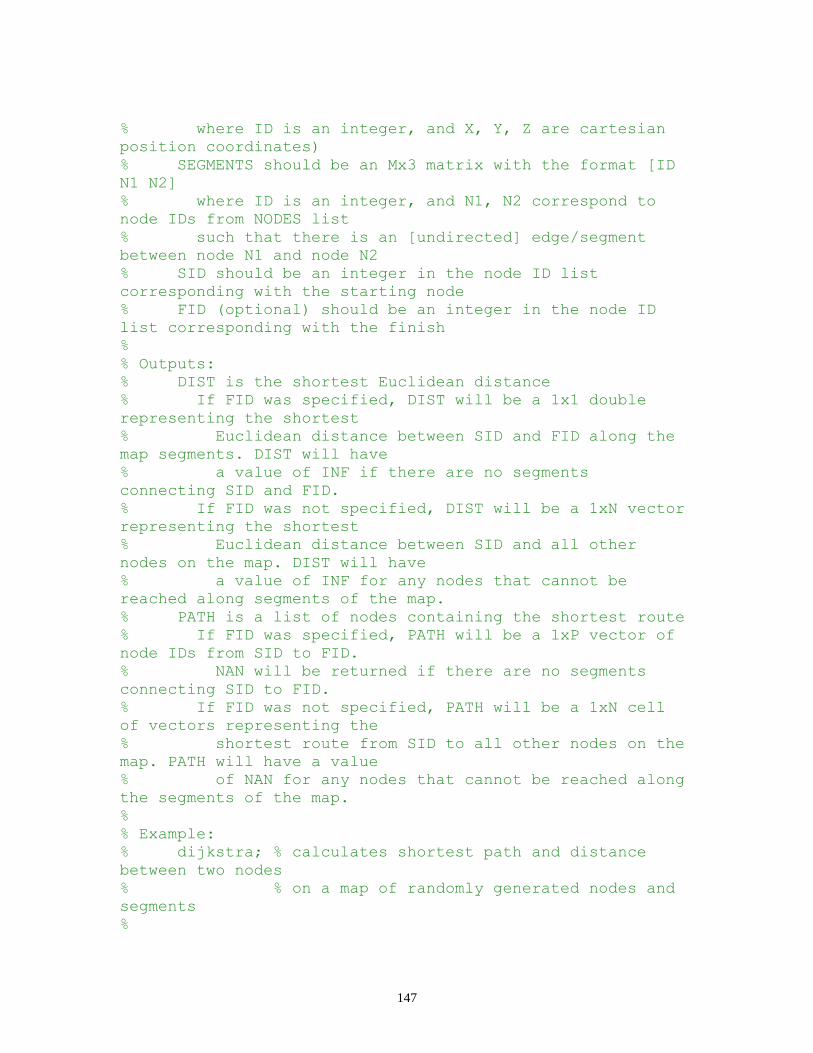
147

% where ID is an integer, and X, Y, Z are cartesian

position coordinates)

% SEGMENTS should be an Mx3 matrix with the format [ID

N1 N2]

% where ID is an integer, and N1, N2 correspond to

node IDs from NODES list

% such that there is an [undirected] edge/segment

between node N1 and node N2

% SID should be an integer in the node ID list

corresponding with the starting node

% FID (optional) should be an integer in the node ID

list corresponding with the finish

%

% Outputs:

% DIST is the shortest Euclidean distance

% If FID was specified, DIST will be a 1x1 double

representing the shortest

% Euclidean distance between SID and FID along the

map segments. DIST will have

% a value of INF if there are no segments

connecting SID and FID.

% If FID was not specified, DIST will be a 1xN vector

representing the shortest

% Euclidean distance between SID and all other

nodes on the map. DIST will have

% a value of INF for any nodes that cannot be

reached along segments of the map.

% PATH is a list of nodes containing the shortest route

% If FID was specified, PATH will be a 1xP vector of

node IDs from SID to FID.

% NAN will be returned if there are no segments

connecting SID to FID.

% If FID was not specified, PATH will be a 1xN cell

of vectors representing the

% shortest route from SID to all other nodes on the

map. PATH will have a value

% of NAN for any nodes that cannot be reached along

the segments of the map.

%

% Example:

% dijkstra; % calculates shortest path and distance

between two nodes

% % on a map of randomly generated nodes and

segments

%

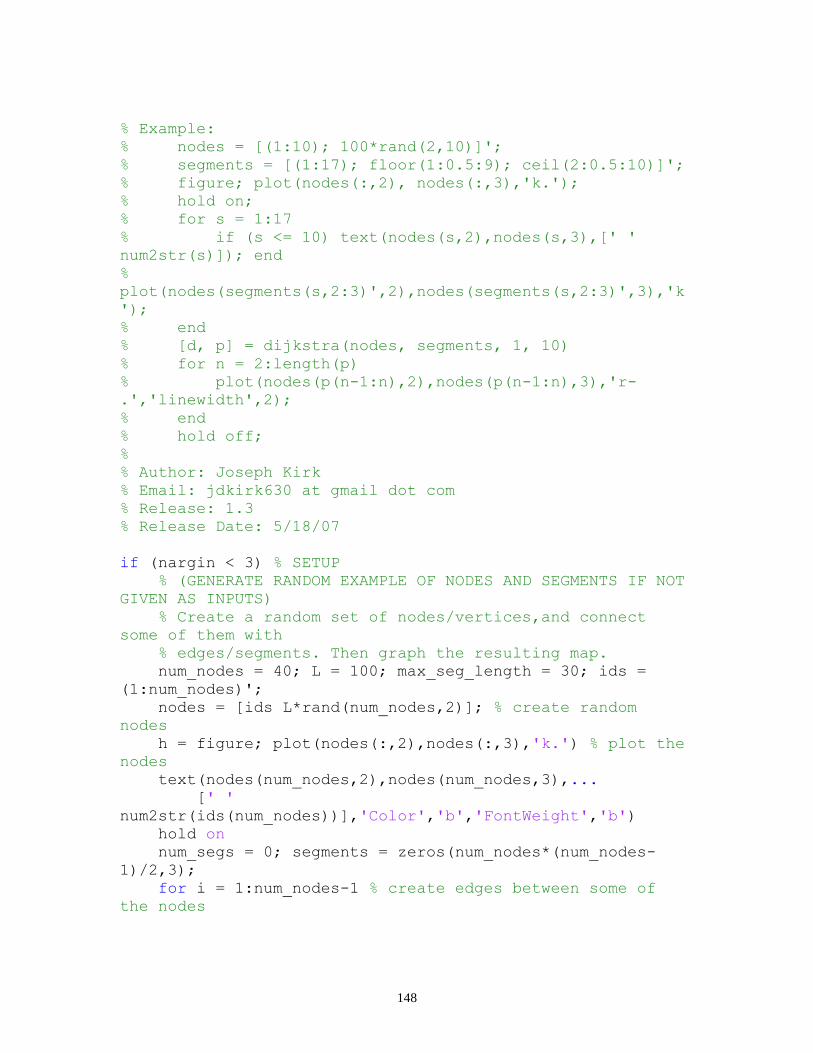
148

% Example:

% nodes = [(1:10); 100*rand(2,10)]';

% segments = [(1:17); floor(1:0.5:9); ceil(2:0.5:10)]';

% figure; plot(nodes(:,2), nodes(:,3),'k.');

% hold on;

% for s = 1:17

% if (s <= 10) text(nodes(s,2),nodes(s,3),[' '

num2str(s)]); end

%

plot(nodes(segments(s,2:3)',2),nodes(segments(s,2:3)',3),'k

');

% end

% [d, p] = dijkstra(nodes, segments, 1, 10)

% for n = 2:length(p)

% plot(nodes(p(n-1:n),2),nodes(p(n-1:n),3),'r-

.','linewidth',2);

% end

% hold off;

%

% Author: Joseph Kirk

% Email: jdkirk630 at gmail dot com

% Release: 1.3

% Release Date: 5/18/07

if (nargin < 3) % SETUP

% (GENERATE RANDOM EXAMPLE OF NODES AND SEGMENTS IF NOT

GIVEN AS INPUTS)

% Create a random set of nodes/vertices,and connect

some of them with

% edges/segments. Then graph the resulting map.

num_nodes = 40; L = 100; max_seg_length = 30; ids =

(1:num_nodes)';

nodes = [ids L*rand(num_nodes,2)]; % create random

nodes

h = figure; plot(nodes(:,2),nodes(:,3),'k.') % plot the

nodes

text(nodes(num_nodes,2),nodes(num_nodes,3),...

[' '

num2str(ids(num_nodes))],'Color','b','FontWeight','b')

hold on

num_segs = 0; segments = zeros(num_nodes*(num_nodes-

1)/2,3);

for i = 1:num_nodes-1 % create edges between some of

the nodes

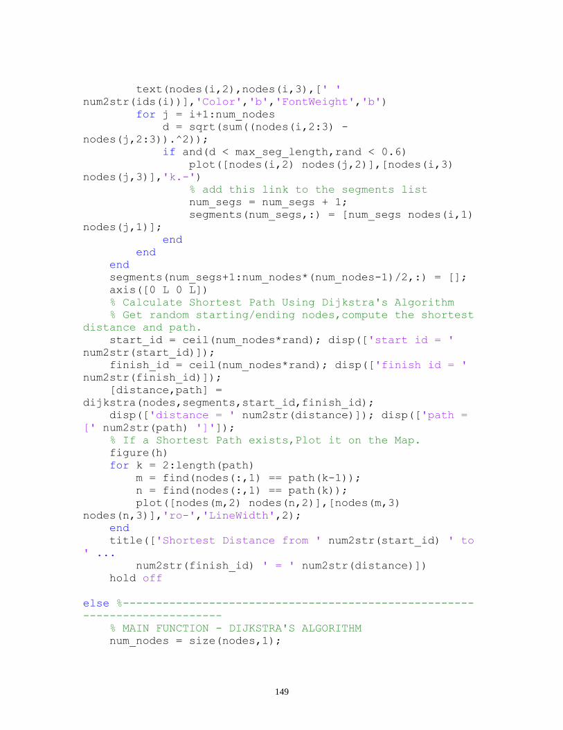
149

text(nodes(i,2),nodes(i,3),[' '

num2str(ids(i))],'Color','b','FontWeight','b')

for j = i+1:num_nodes

d = sqrt(sum((nodes(i,2:3) -

nodes(j,2:3)).^2));

if and(d < max_seg_length,rand < 0.6)

plot([nodes(i,2) nodes(j,2)],[nodes(i,3)

nodes(j,3)],'k.-')

% add this link to the segments list

num_segs = num_segs + 1;

segments(num_segs,:) = [num_segs nodes(i,1)

nodes(j,1)];

end

end

end

segments(num_segs+1:num_nodes*(num_nodes-1)/2,:) = [];

axis([0 L 0 L])

% Calculate Shortest Path Using Dijkstra's Algorithm

% Get random starting/ending nodes,compute the shortest

distance and path.

start_id = ceil(num_nodes*rand); disp(['start id = '

num2str(start_id)]);

finish_id = ceil(num_nodes*rand); disp(['finish id = '

num2str(finish_id)]);

[distance,path] =

dijkstra(nodes,segments,start_id,finish_id);

disp(['distance = ' num2str(distance)]); disp(['path =

[' num2str(path) ']']);

% If a Shortest Path exists,Plot it on the Map.

figure(h)

for k = 2:length(path)

m = find(nodes(:,1) == path(k-1));

n = find(nodes(:,1) == path(k));

plot([nodes(m,2) nodes(n,2)],[nodes(m,3)

nodes(n,3)],'ro-','LineWidth',2);

end

title(['Shortest Distance from ' num2str(start_id) ' to

' ...

num2str(finish_id) ' = ' num2str(distance)])

hold off

else %-----------------------------------------------------

---------------------

% MAIN FUNCTION - DIJKSTRA'S ALGORITHM

num_nodes = size(nodes,1);

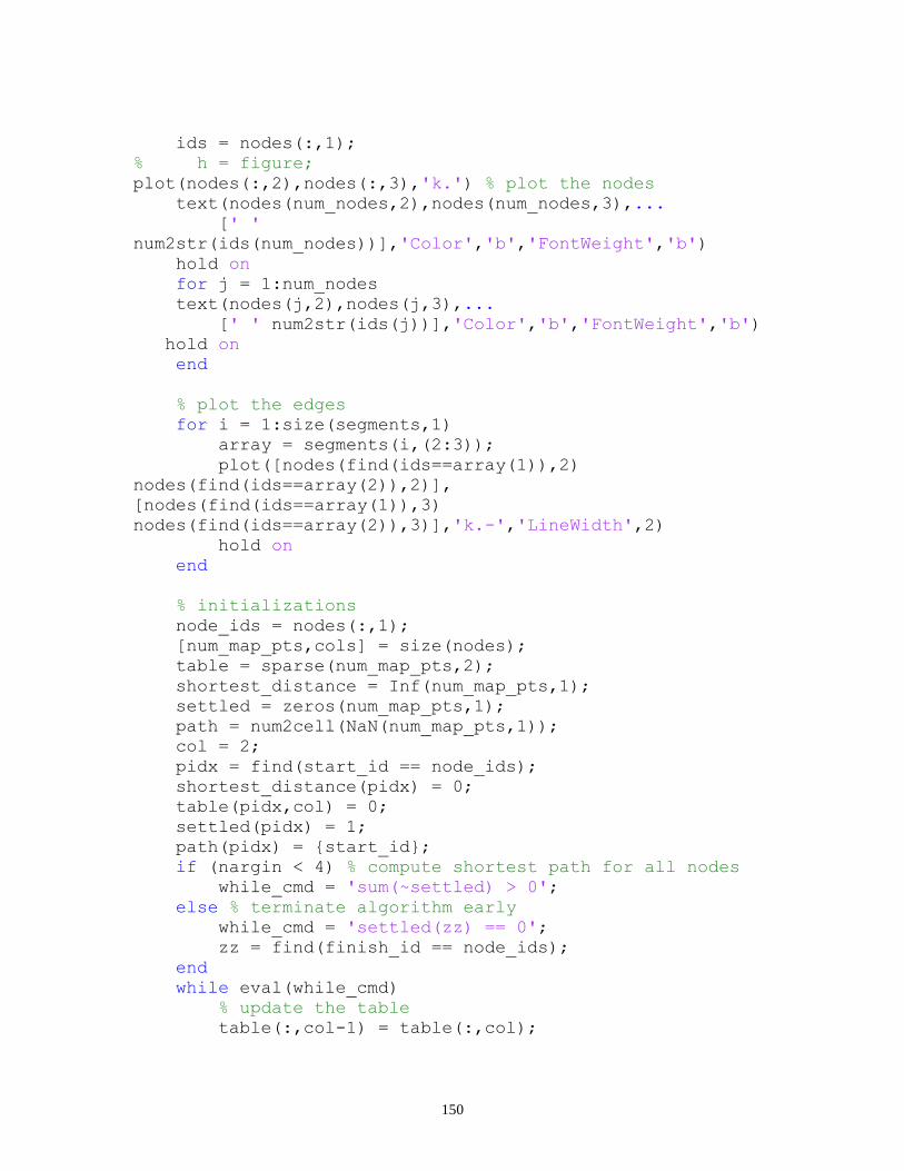
150

ids = nodes(:,1);

% h = figure;

plot(nodes(:,2),nodes(:,3),'k.') % plot the nodes

text(nodes(num_nodes,2),nodes(num_nodes,3),...

[' '

num2str(ids(num_nodes))],'Color','b','FontWeight','b')

hold on

for j = 1:num_nodes

text(nodes(j,2),nodes(j,3),...

[' ' num2str(ids(j))],'Color','b','FontWeight','b')

hold on

end

% plot the edges

for i = 1:size(segments,1)

array = segments(i,(2:3));

plot([nodes(find(ids==array(1)),2)

nodes(find(ids==array(2)),2)],

[nodes(find(ids==array(1)),3)

nodes(find(ids==array(2)),3)],'k.-','LineWidth',2)

hold on

end

% initializations

node_ids = nodes(:,1);

[num_map_pts,cols] = size(nodes);

table = sparse(num_map_pts,2);

shortest_distance = Inf(num_map_pts,1);

settled = zeros(num_map_pts,1);

path = num2cell(NaN(num_map_pts,1));

col = 2;

pidx = find(start_id == node_ids);

shortest_distance(pidx) = 0;

table(pidx,col) = 0;

settled(pidx) = 1;

path(pidx) = {start_id};

if (nargin < 4) % compute shortest path for all nodes

while_cmd = 'sum(~settled) > 0';

else % terminate algorithm early

while_cmd = 'settled(zz) == 0';

zz = find(finish_id == node_ids);

end

while eval(while_cmd)

% update the table

table(:,col-1) = table(:,col);

151

table(pidx,col) = 0;

% find neighboring nodes in the segments list

neighbor_ids = [segments(node_ids(pidx) ==

segments(:,2),3);

segments(node_ids(pidx) == segments(:,3),2)];

% calculate the distances to the neighboring nodes

and keep track of the paths

for k = 1:length(neighbor_ids)

cidx = find(neighbor_ids(k) == node_ids);

if ~settled(cidx)

d = sqrt(sum((nodes(pidx,2:cols) -

nodes(cidx,2:cols)).^2));

if (table(cidx,col-1) == 0) || ...

(table(cidx,col-1) >

(table(pidx,col-1) + d))

table(cidx,col) = table(pidx,col-1) +

d;

tmp_path = path(pidx);

path(cidx) = {[tmp_path{1}

neighbor_ids(k)]};

else

table(cidx,col) = table(cidx,col-1);

end

end

end

% find the minimum non-zero value in the table and

save it

nidx = find(table(:,col));

ndx = find(table(nidx,col) ==

min(table(nidx,col)));

if isempty(ndx)

break

else

pidx = nidx(ndx(1));

shortest_distance(pidx) = table(pidx,col);

settled(pidx) = 1;

end

end

if (nargin < 4) % return the distance and path arrays

for all of the nodes

dist = shortest_distance';

path = path';

else % return the distance and path for the ending node

dist = shortest_distance(zz);

path = path(zz);

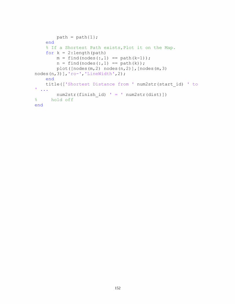
152

path = path{1};

end

% If a Shortest Path exists,Plot it on the Map.

for k = 2:length(path)

m = find(nodes(:,1) == path(k-1));

n = find(nodes(:,1) == path(k));

plot([nodes(m,2) nodes(n,2)],[nodes(m,3)

nodes(n,3)],'ro-','LineWidth',2);

end

title(['Shortest Distance from ' num2str(start_id) ' to

' ...

num2str(finish_id) ' = ' num2str(dist)])

% hold off

end

153

REFERENCES

[1] Dandurand, B., Guarneri, P., Fadel, G. M., and Wiecek, M. M., 2014, “Bi-level

Multibjective Packaging Optimization for Automotive Design,” J. Mech. Des.,

(November 2013).

[2] Wodziak, J. R., and Fadel, G. M., 1994, “Packing and optimizing the center of

gravity location using a genetic algorithm,” J. Comput. Ind., 11, pp. 2–14.

[3] Grignon, P. M., and Fadel, G. M., 1999, “CONFIGURATION DESIGN

OPTIMIZATION METHOD,” Proceedings of DETC99 1999 ASME Design

Engineering Technical Conferences September 12–15, 1999, Las Vegas, Nevada,

pp. 1–13.

[4] Miao, Y., Blouin, V. Y., and Fadel, G. M., 2003, “Multi-objective configuration

optimization with vehicle dynamics applied to midsize truck design,” Proceedings

of ASME, pp. 319–327.

[5] Dong, H., Fadel, G. M., and Blouin, V. Y., 2005, “Packing optimization by

enhanced rubber band analogy,” ASME International Design Engineering

Technical Conferences and Computers and Information in Engineering

Conference, Long Beach, California. 2005, pp. 1–9.

[6] Tiwari, S., Fadel, G., and Fenyes, P., 2008, “A fast and efficient compact packing

algorithm for free-form objects,” Proceedings of the ASME International Design

Engineering Technical Conferences & Computers and Information in Engineering

Conference, New York, ASME Paper No. DETC2008-50097.

[7] Katragadda, R. T., Gondipalle, S. R., Guarneri, P., and Fadel, G., 2012,

“Predicting the thermal performance for the multi-objective vehicle underhood

packing optimization problem,” Proceedings of ASME DETC, pp. 1–8.

[8] Matheus, K., and Konigseder, T., 2015, Automotive Ethernet, Cambridge

University Press.

[9] Latombe, J.-C., 1991, Robot Motion Planning, Kluwer Academic Publishers,

Boston.

[10] Bhattacharya, B. Y. P., and Gavrilova, M. L., 2008, “Roadmap-Based Path

Planning,” (June).

[11] Amato, N. M., and Wu, Y., 1996, “A Randomized Roadmap Method for Path and

Manipulation Planning,” IEEE International Conference on Robotics and

Automation, pp. 113–120.

[12] Borenstein, J., and Koren, Y., 1989, “Real-time obstacle avoidance for fast mobile

robots,” {IEEE} {T}ransactions on {S}ystems, {M}an, & {C}ybernetics, 19(5),

pp. 1179–1187.

[13] Sandurkar, S., and Chen, W., 1999, “GAPRUS - genetic algorithms based pipe

routing using tessellated objects,” Comput. Ind., 38(3), pp. 209–223.

[14] O’Rourke, J., and Mallinckrodt, A. J., 1995, Computational Geometry in C,

Computers in Physics.

154

[15] Asano, T., Asano, T., Guibas, L., Hershberger, J., and Imai, H., 1985, “Visibility-

Polygon Search and Euclidean Shortest Paths,” Found. Comput. Sci., pp. 155–164.

[16] Rohnert, H., 1986, “Shortest Paths in the Plane with Convex Polygonal Obstacles,”

Information, 23, pp. 71–76.

[17] Fredman, M. L., and Tarjan, R. E., 1987, “Fibonacci heaps and their uses in

improved network optimization algorithms.pdf,” J. ACM, 34.3, pp. 596–615.

[18] Welzl, E., 1985, “CONSTRUCTING THE VISIBILITY GRAPH FOR n-LINE

SEGMENTS IN O(n 2) TIME,” Inf. Process. Lett., pp. 167–171.

[19] Sharir, M., and Schorr, A., 1986, “On shortest paths in polyhedral Spaces,” SIAM

J. Comput., 15.1(1), pp. 193–215.

[20] Aho, A. V., and Hopcroft, J. E., 1974, “Design and Analysis of Computer

Algorithms,” Pearson Education India.

[21] Butt, S. E., and Cavalier, T. M., 1996, “An efficient algorithm for facility location

in the presence of forbidden regions,” Eur. J. Oper. Res., 90(1), pp. 56–70.

[22] Lozano-Pérez, T., and Wesley, M. a., 1979, “An algorithm for planning collision-

free paths among polyhedral obstacles,” Commun. ACM, 22(10), pp. 560–570.

[23] Meeran, S., and Shafie, A., 1997, “O P T I M U M PATH PLANNING USING

CONVEX HULL AND LOCAL SEARCH HEURISTIC ALGORITHMS,”

Mechatronics, 7(8), pp. 737–756.

[24] Flood, M. M. ., 1956, “The Traveling Salesman Problem,” Oper. Res., 4(1), pp.

61–75.

[25] Bhattacharya, P., Tnn, C., and Gavrilova, M. L., 2007, “Geometric Algorithms for

Clearance Based Optimal Path Computation,” pp. 1–4.

[26] Dijkstra, E. W., 1959, “A note on two problems in connexion with graphs.pdf,”

Numer. Math., pp. 269–271.

[27] Wein, R., and Halperin, D., 2005, “The Visibility – Voronoi Complex and Its

Applications,” Proc. twenty-first Annu. Symp. Comput. Geom., pp. 63–72.

[28] Clarkson, K., 1987, “Approximation algorithms for shortest path motion

planning,” Proc. Ninet. Annu. ACM Symp. Theory Comput., pp. 56–65.

[29] Hershberger, J., and Suri, S., 1999, “An Optimal Algorithm for Euclidean Shortest

Paths in the Plane,” SIAM J. Comput., 28(6), pp. 2215–2256.

[30] Yin, Y. H., Zhou, C., and Zhu, J. Y., 2010, “A pipe route design methodology by

imitating human imaginal thinking,” CIRP Ann. - Manuf. Technol., 59(1), pp.

167–170.

[31] Szykman, S., and Cagan, J., 1996, “Synthesis of Optimal Nonorthogonal

Routes.pdf,” J. Mech. Des., 118(3), pp. 419–424.

[32] Gottschalk, S., Lin, M. C., Manocha, D., and Hill, C., 1996, “OBBTree: A

Hierarchical Structure for Rapid Interference Detection,” Proceedings of the 23rd

annual conference on Computer graphics and interactive techniques. ACM, pp.

171–180.

[33] Conru, A. B., and Cutkosky, M. R., 1993, “Computational Support for Interactive

155

Cable Harness Routing and Design,” Adv. Des. Autom., 1, pp. 551–558.

[34] Conru, A. B., 1994, “A genetic approach to the cable harness routing problem,”

Ieee, pp. 200–205.

[35] Lin, C., Rao, L., Giusto, P., Ambrosio, J. D., and Sangiovanni-vincentelli, A.,

2014, “An Efficient Wire Routing and Wire Sizing Algorithm for Weight

Minimization of Automotive Systems,” Proceedings of the 51st Annual Design

Automation Conference. ACM, pp. 1–6.

[36] Lin, C., Rao, L., Ambrosio, J. D., and Sangiovanni-vincentelli, A., 2014,

“Electrical Architecture Optimization and Selection - Cost Minimization via Wire

Routing and Wire Sizing,” SAE Int. J. Passeng. Cars-Electronic Electr. Syst., pp.

502–509.

[37] Zhu, Z., 2017, “A methodology to enable automatic 3D routing of aircraft

Electrical Wiring Interconnection System,” CEAS Aeronaut. J., 8(2), pp. 287–302.

[38] Chen, D. Z., 2017, “Developing Algorithms and Software for Geometric Path

Planning Problems,” 28(December 1996), pp. 1–5.

[39] Zeid, I., 2005, Mastering CAD/CAM, Mc Graw Hill.

[40] Fadel, G. M., Kirschman, C., and Kirschman, C., 1996, “Accuracy issues in CAD

to RP translations,” Rapid Prototyp. J.

[41] Liu, E. P., and Carey, R., 1998, “The Virtual Reality Modeling Language

Explained,” IEEE Multimed., 5(3), pp. 84–93.

[42] “Multidemnsional Arrays” [Online]. Available:

https://www.mathworks.com/help/matlab/math/multidimensional-arrays.html#f1-

87418.

[43] Aurenhammer, F., 1991, “Voronoi Diagrams — A Survey of a Fundamental Data

Structure,” 23(3).

[44] K, S., 1993, “Approximation of Generalized Voronoi Diagrams by Ordinary

Voronoi Diagrams,” CVGIP Graph. Model. Image Process., 55 (6), pp. 522–531.

[45] Mounts, D. M., 1991, “AN OUTPUT SENSITIVE ALGORITHM FOR

COMPUTING VISIBILITY GRAPHS *,” 20(5), pp. 888–910.

[46] Sniedovich, M., 2006, “Dijkstra ’ s algorithm revisited : the dynamic programming

connexion by,” 35(3), pp. 87–92.

[47] 2009, “Lecture 18 Solving Shortest Path Problem : Dijkstra ’ s Algorithm”

[Online]. Available:

http://www.ifp.illinois.edu/~angelia/ge330fall09_dijkstra_l18.pdf.

Geometric Path-Planning Algorithm in Cluttered 2D ...

Documents