Geometric and transformational properties of Lipschitz domains, Semmes-Kenig-Toro domains, and other classes of finite perimeter domains

Geometric and Transformational Properties of Lipschitz Domains,

Semmes-Kenig-Toro Domains, and Other Classes of Finite

Perimeter Domains ∗

Steve Hofmann, Marius Mitrea and Michael Taylor

Abstract

In the first part of this paper we give intrinsic characterizations of the classes of Lipschitz andC1 domains. Under some mild, necessary, background hypotheses (of topological and geometricmeasure theoretic nature), we show that a domain is Lipschitz if and only if it has a continuoustransversal vector field. We also show that if the geometric measure theoretic unit normal ofthe domain is continuous, then the domain in question is of class C1. In the second part of thepaper, we study the invariance of various classes of domains of locally finite perimeter under bi-Lipschitz and C1 diffeomorphisms of the Euclidean space. In particular, we prove that the classof bounded regular SKT domains (previously called chord-arc domains with vanishing constant,in the literature) is stable under C1 diffeomorphisms. A number of other applications are alsopresented.

1 Introduction

Analysis on rough domains has become a prominent area of research over the past few decades.Much of the literature has been devoted to domains in Euclidean space with rough boundary,such as Lipschitz domains and chord-arc domains. However, as treatments of partial differentialequations with variable coefficients on such domains has advanced, it has become natural as wellas geometrically significant to work on rough domains in Riemannian manifolds. Works on thisinclude [18], [17], and [10], among others. The original definitions of various classes of domains,such as strongly Lipschitz domains, are tied to the linear structure of Euclidean space, and therearises the issue of how to define such classes of domains in the manifold setting.

One viable approach, taken in the papers mentioned above, is to call an open set Ω in a smoothmanifold M locally strongly Lipschitz (for example) if for each p ∈ ∂Ω there exists a smoothcoordinate chart on a neighborhood U of p such that ∂Ω∩U is a Lipschitz graph in this coordinatesystem. One can give similar definitions of chord-arc domains in M , etc. However, this approachleaves aside a number of interesting issues, which we take up in this paper. These issues centerabout whether one can establish the invariance of various classes of rough domains (with their

∗2000 Math Subject Classification. Primary: 49Q15, 26B15, 49Q25 Secondary 26A16, 26A66, 26B30

Key words: locally strongly Lipschitz domains, C1 domains, transversal fields, bi-Lipschitz maps, C

1 diffeomorphisms,

sets of locally finite perimeter, unit normal, surface area

The work of authors was supported in part by NSF grants DMS-0245401, DMS-0653180, DMS-FRG0456306, and

DMS-0456861

1

original definitions) under C1-diffeomorphisms (and, for certain classes of finite perimeter domains,even under bi-Lipschitz maps), and, closely related, whether one can provide intrinsic geometricalcharacterizations of Lipschitz domains and other classes.

The first issue we treat here is the characterization of locally strongly Lipschitz domains as thosedomains Ω of locally finite perimeter for which there are continuous (or, equivalently, smooth) vectorfields that are transverse to the boundary, and that also satisfy the necessary, mild topologicalcondition ∂Ω = ∂Ω. See §2 for the definition of transverse in this setting. The fact that stronglyLipschitz domains possess such transverse vector fields is well known, and has played a significantrole in analysis on this class of domains. Results of §2 establish the converse.

The analytical significance of the existence of such transversal vector fields is that it leads toRellich identities. Excellent illustrations of the use of these identities include [11], giving estimates

on harmonic measure, and [20], providing boundary Garding inequalities in strongly Lipschitz

domains. Another case where the use of transversal vector fields arises is to establish the invertibilityof boundary integral operators of layer potential type on strongly Lipschitz domains, starting with[24]. In this case the Rellich identities are applied in concert with two other tools:

(a) Green formulas for appropriate classes of functions on strongly Lipschitz domains;

(b) The Calderon-Coifman-McIntosh-Meyer theory for singular integral operators on stronglyLipschitz surfaces.

These tools permit one to reduce various elliptic boundary problems to certain boundary integralequations, and to solve these equations.

In recent years, (a) and (b) above have been extended to a much more general class of domainsthan that of Lipschitz domains. See, e.g., [8], [16] for (a), and [4], [5] for (b). Quite recently, in [10],we have further refined some of these results and used them to treat boundary value problems inchord-arc domains with vanishing constant (in the terminology of [14], [15]), which we call regularSKT domains. (See §5 for a definition.) It follows from the characterization stated above thatthere is not a corresponding extension of the use of transverse vector fields to a class of domainsbigger than the class of strongly Lipschitz domains, so one will need to seek other methods to addto (a) and (b) to tackle elliptic boundary problems on such domains, as has been done in the caseof regular SKT domains in [10].

Among other results established in §2, we mention the following. Let Ω ⊂ Rn be a bounded,nonempty, open set of finite perimeter for which ∂Ω = ∂Ω, and denote by ν, σ, respectively, the(geometric measure theoretic) outward unit normal and surface measure on ∂Ω. Then the quantity

ρ(Ω) := inf ‖ν − f‖L∞(∂Ω,dσ) : f ∈ C0(∂Ω,Rn), |f | = 1 on ∂Ω (1.1)

can be used to characterize the membership of Ω both in the class of strongly Lipschitz domainsand in the class of C1 domains. Specifically,

Ω is a strongly Lipschitz domain ⇐⇒ ρ(Ω) <√

2, (1.2)

Ω is a C1-domain ⇐⇒ ρ(Ω) = 0. (1.3)

This can be compared with the recent result proved in [10], to the effect that for a bounded NTAdomain, with an Ahlfors regular boundary (cf. § 5 for the relevant terminology),

2

Ω is a regular SKT domain ⇐⇒ inf ‖ν − f‖BMO(∂Ω,dσ) : f ∈ C0(∂Ω,Rn) = 0. (1.4)

Section 3 studies the images of locally finite perimeter domains in Rn. We show that this classof domains is invariant under bi-Lipschitz maps. If Ω is such a domain and F is a map that is notonly bi-Lipschitz but actually a C1 diffeomorphism, we relate the (measure-theoretic) outward unitnormal ν and surface measure σ on ∂Ω to the outward unit normal ν and surface measure σ on∂F (Ω). Specifically, here we prove that

ν =(DF−1)>(ν F−1)

‖(DF−1)>(ν F−1)‖ and (1.5)

σ = ‖(DF−1)>(ν F−1)‖ |det (DF ) F−1|F∗σ, (1.6)

where DF is the Jacobian matrix of F , and F∗σ denotes the push-forward of the measure σ viathe mapping F .

In §4 we use this result together with the transversality characterization from §2, to prove theinvariance of the class of locally strongly Lipschitz domains under C 1 diffeomorphisms. Here, asin §§2–3, most of our work is done for domains in Euclidean space Rn, but once these invarianceresults are established, their analogues in the manifold setting are fairly straightforward. Forexample, both the class of Lipschitz domains, as well as the class of regular SKT domains, havenatural definitions in the setting of manifolds, which rely only on the intrinsic C 1 structure of themanifold.

Other topics treated in §4 include the recollection of several examples of bi-Lipschitz mapstaking bounded strongly Lipschitz domains to domains which fail to be, themselves, strongly Lip-schitz. We then proceed to establish the invariance of the class of regular SKT domains underC1 diffeomorphisms. Furthermore, making use of (1.5)-(1.6), we devise a general approximationscheme for domains of locally finite perimeter. When specialized to the case of bounded stronglyLipschitz domains, this yields an approximation result akin to the work of A.P. Calderon in [2].

Section 5 is an appendix, consisting of three subsections. The purpose of the first, is to collectdefinitions and basic properties of SKT domains and regular SKT domains, needed for applicationin §4. In the second subsection, we deduce a number of useful formulas in linear algebra, used in§2, and in §5.3 we collect a number of useful results in elementary topology.

The overall plan of the remainder of the paper is as follows:

2. Finite perimeter domains with continuous transversal fields3. Finite perimeter domains under bi-Lipschitz and C 1 diffeomorphisms4. Further applications

4.1 Bounded Lipschitz domains are invariant under C 1 diffeomorphisms4.2 Regular SKT domains are invariant under C1 diffeomorphisms4.3 Approximating domains of locally finite perimeter

5. Appendix5.1 Reifenberg flat, nontangentially accessible, and Semmes-Kenig-Toro domains5.2 Cross products and determinants5.3 Some topological lemmas

3

2 Finite perimeter domains with continuous transversal fields

Throughout this paper, we shall assume that n ≥ 2 is a fixed integer. Call an open set Ω ⊂ Rn oflocally finite perimeter provided

µ := ∇1Ω (2.1)

is a locally finite Rn-valued measure. (Hereafter, we denote by 1E the characteristic function of aset E.) For a domain of locally finite perimeter which has a compact boundary we agree to dropthe adverb ‘locally’. Given an open set Ω ⊂ Rn of locally finite perimeter we denote by σ the totalvariation measure of µ; σ is then a locally finite positive measure, supported on ∂Ω, and clearly eachcomponent of µ is absolutely continuous with respect to σ. It follows from the Radon-Nikodymtheorem that

µ = ∇1Ω = −νσ, (2.2)

where

ν ∈ L∞(∂Ω, dσ) is an Rn-valued function, satisfying |ν(x)| = 1, for σ-a.e. x ∈ ∂Ω (2.3)

In the sequel, we shall frequently identify σ with its restriction to ∂Ω, with no special mention. Weshall refer to ν and σ, respectively, as the (geometric measure theoretic) outward unit normal andthe surface measure on ∂Ω.

Note that ν defined by (2.2) can only be specified up to a set of σ-measure zero. To eliminatethis ambiguity, we redefine ν(x), for every x, as being

limr→0

∫−

B(x,r)ν dσ (2.4)

whenever the limit exists, and zero otherwise. In doing so, the following convention is employed. Weset∫−B(x,r)ν dσ := (σ(B(x, r)))−1

∫B(x,r) ν dσ if σ(B(x, r)) > 0, and zero otherwise. The Besicovitch

Differentiation Theorem (cf., e.g., [7]) ensures that ν in (2.2) agrees with (2.4) for σ-a.e. x.The reduced boundary of Ω is then defined as

∂∗Ω :=x : |ν(x)| = 1

. (2.5)

This is essentially the point of view adopted in [26] (cf. Definition 5.5.1 on p. 233). Let us remarkthat this definition is slightly different from that given on p. 194 of [7]. The reduced boundaryintroduced there depends on the choice of the unit normal in the class of functions agreeing with itσ-a.e. and, consequently, can be pointwise specified only up to a certain set of zero surface measure.Nonetheless, any such representative is a subset of our ∂∗Ω and differs from it by a set of σ-measurezero.

Moving on, it follows from (2.5) and the Besicovitch Differentiation Theorem that σ is supportedon ∂∗Ω, in the sense that σ(Rn \ ∂∗Ω) = 0. From the work of Federer and of De Giorgi it is alsoknow that, if Hn−1 is the (n− 1)-dimensional Hausdorff measure in Rn,

4

σ = Hn−1b∂∗Ω. (2.6)

Recall that, generally speaking, given a Radon measure µ in Rn and a set A ⊂ Rn, the restrictionof µ to A is defined as µ bA := 1A µ. In particular, µ bA << µ and d(µ bA)/dµ = 1A. Thus,

σ << Hn−1 anddσ

dHn−1= 1∂∗Ω. (2.7)

Furthermore (cf. Lemma 5.9.5 on p. 252 in [26], and p. 208 in [7]) one has

∂∗Ω ⊆ ∂∗Ω ⊆ ∂Ω, and Hn−1(∂∗Ω \ ∂∗Ω) = 0, (2.8)

where ∂∗Ω, the measure-theoretic boundary of Ω, is defined by

∂∗Ω :=x ∈ ∂Ω : lim sup

r→0+

r−nHn(B(x, r) ∩ Ω±) > 0

. (2.9)

Above, Hn denotes n-dimensional Hausdorff measure (i.e., the Lebesgue measure) in Rn, and wehave set Ω+ := Ω, Ω− := Rn \ Ω (later on, instead of Ω− we shall use the notation Ωc). Let usalso record here a useful criterion for deciding whether a Lebesgue measurable subset E of Rn is oflocally finite perimeter in Rn (cf. [7], p. 222):

E has locally finite perimeter ⇐⇒ Hn−1(∂∗E ∩K) <∞, ∀K ⊂ Rn, compact. (2.10)

A moment’s reflection shows that this can be rephrased as

E has locally finite perimeter ⇐⇒ ∀x ∈ ∂E ∃ r > 0 so that Hn−1(∂∗E ∩B(x, r)) <∞. (2.11)

Definition 2.1. Let Ω ⊂ Rn be an open set of locally finite perimeter, with outward unit nor-mal ν and surface measure σ, and a point x0 ∈ ∂Ω. Then, it is said that Ω has a continuous

transversal vector field near x0 provided there exist r > 0, κ > 0 and a continuous vectorfield X on B(x, r) ∩ ∂Ω which is (outwardly) transverse to ∂Ω near x0, in the sense that

ν ·X ≥ κ σ-a.e. on B(x, r) ∩ ∂Ω. (2.12)

Next, it is said that Ω has continuous transversal vector fields provided Ω has a continuous

transversal vector field near x for each point x ∈ ∂Ω.Finally, Ω is said to have continuous globally transversal vector fields if there exist

a vector field X ∈ C0(∂Ω,Rn) and a number κ > 0 (called the transversality constant of X) withthe property that ν ·X ≥ κ at σ-a.e. point on ∂Ω.

Lemma 2.1. Assume that Ω ⊂ Rn is a domain of finite perimeter, whose boundary is compact,and which has continuous locally transversal vector fields. Then Ω has, in fact, global continuoustransversal vector fields.

5

Proof. The argument is standard. From compactness, there exist xj ∈ ∂Ω, rj , κj > 0, 1 ≤ j ≤ m,along with Xj ∈ C0(B(xj , rj) ∩ ∂Ω,Rn), 1 ≤ j ≤ m, with the property that ∂Ω ⊆ ⋃

1≤j≤mB(xj, rj),

and ν ·Xj ≥ κj at σ-a.e. point on B(xj, rj)∩∂Ω, for each j = 1, ...,m. If we now consider ψj1≤j≤m,a partition of unity in a neighborhood of ∂Ω consisting of smooth, nonnegative functions for whichsuppψj ⊂ B(xj , rj), 1 ≤ j ≤ m, then X :=

∑mj=1 ψjXj ∈ C0(∂Ω,Rn) satisfies

ν ·X =m∑

j=1

ψj ν ·Xj ≥m∑

j=1

κjψj ≥ κ, (2.13)

where κ := min κ1, ..., κm > 0. Thus, Ω has global continuous transversal vector fields.

Below we collect several equivalent formulations of the above definition. Here and elsewhere, weshall denote the standard norm in Rn by either | · |, or ‖·‖. Also, C0, C1, ..., C∞ stand, respectively,for the classes of continuous functions, continuously differentiable functions, ... , infinitely manytimes differentiable functions.

Proposition 2.2. For an open set of locally finite perimeter, Ω ⊂ Rn, the following two conditionsare equivalent:

(i) Ω has continuous locally transversal vector fields;

(ii) for every point x ∈ ∂Ω there exist r > 0, κ > 0 and X ∈ C∞(Rn,Rn) such that (2.12) holds.

Furthermore, the local versions of (i)-(ii) above are also equivalent.If the domain Ω also satisfies

Hn−1(∂∗Ω ∩B(x, r)) > 0, ∀x ∈ ∂Ω, ∀ r > 0, (2.14)

then (i)-(ii) above are also equivalent to:

(iii) for every x ∈ ∂Ω there exist κ > 0, r > 0 and X ∈ C∞(Rn,Rn) such that |X| = 1 onB(x, r/2) ∩ ∂Ω and (2.12) holds.

Granted (2.14), then the local versions of (i)-(ii) are equivalent with the local version of (iii).Finally, if additionally to (2.14), ∂Ω is compact, then (i)-(iii) above are also equivalent to:

(iv) there exists X ∈ C∞(Rn,Rn) which is globally transversal to Ω and such that |X| = 1 on ∂Ω;

(v) there exists X ∈ C0(∂Ω,Rn) satisfying |X| = 1 on ∂Ω and ‖ν −X‖L∞(∂Ω,dσ) <√

2, where ν,σ stand, respectively, for the outward unit normal and surface measure on ∂Ω.

Proof. The fact that (i) ⇔ (ii) is an easy consequence of the fact that small L∞ perturbations of atransversal fields are also transversal, plus a standard mollification argument. The same argumentalso works for the local versions of (i) and (ii). To further show that (ii) ⇔ (iii), note that (2.14)and (2.6)-(2.8) imply

σ(B(x, r) ∩ ∂Ω) > 0, ∀x ∈ ∂Ω, ∀ r > 0. (2.15)

6

Hence, a continuous field satisfying (2.12) cannot vanish on B(x, r) ∩ ∂Ω, since this would violate(2.15). Consequently, if X is as in (ii), then its (pointwise) normalized version remains transversalto Ω on B(x, r/2) ∩ ∂Ω. If ∂Ω is compact, Lemma 2.1 shows that there exists X ∈ C∞(∂Ω,Rn)which is globally transversal to ∂Ω. Then the same reasoning as above proves that X can benormalized to unit on ∂Ω. This takes care of the claim made about (iv). As for (v), it suffices toobserve that if X ∈ C0(∂Ω,Rn) satisfies |X| = 1 on ∂Ω, then ν ·X = 1

2(2− |ν−X|2) pointwise a.e.

on ∂Ω. Thus, the field X is globally transversal to ∂Ω if and only if ‖ν −X‖L∞(∂Ω,dσ) <√

2.

Remark. It is worth pointing out that, for a set Ω ⊆ Rn of locally finite perimeter, condition (2.14)is equivalent to

∂∗Ω is dense in ∂Ω. (2.16)

Indeed, on the one hand, it is clear that (2.14) implies (2.16). On the other hand, it is known thatfor each x ∈ ∂∗Ω

0 < C1 ≤ lim infr→0+

r1−nσ(B(x, r) ∩ ∂Ω) ≤ lim supr→0+

r1−nσ(B(x, r) ∩ ∂Ω) ≤ C2 <∞, (2.17)

for some dimensional constants C1, C2 (cf. Lemma 2 on p. 196 in [7]). It is then easy to derive (2.14)based on (2.16) and (2.17) (for this, (2.6)- (2.8) are also useful). Furthermore, a slight variation ofthe argument above shows that (2.14) is further equivalent to ∂∗Ω being dense in ∂Ω.

A large class of domains for which continuous locally transversal fields exist is the collectionof all strongly Lipschitz domains in Rn, with compact boundary. For the clarity of the expositionwe record here a formal definition (recall that the superscript c is the operation of taking thecomplement of a set, relative to Rn).

Definition 2.2. Let Ω be a nonempty, proper open subset of Rn. Also, fix x0 ∈ ∂Ω. Call Ω astrongly Lipschitz domain near x0 if there exist b, c > 0 with the following significance. Thereexist an (n − 1)-plane H ⊂ Rn passing through x0, a choice N of the unit normal to H, and anopen cylinder Cb,c := x′ + tN : x′ ∈ H, |x′ − x0| < b, |t| < c (called coordinate cylinder near x0)such that

Cb,c ∩ Ω = Cb,c ∩ x′ + tN : x′ ∈ H, t > ϕ(x′), (2.18)

Cb,c ∩ ∂Ω = Cb,c ∩ x′ + tN : x′ ∈ H, t = ϕ(x′), (2.19)

Cb,c ∩ Ωc= Cb,c ∩ x′ + tN : x′ ∈ H, t < ϕ(x′), (2.20)

for some Lipschitz function ϕ : H → R satisfying

ϕ(x0) = 0 and |ϕ(x′)| < d if |x′ − x0| ≤ b. (2.21)

Finally, call Ω a locally strongly Lipschitz domain if it is a locally strongly Lipschitz domainnear every point x ∈ ∂Ω.

7

Remarks. (i) It should be noted that the conditions (2.18)-(2.20) are not independent since, in fact,(2.18) implies (2.19)-(2.20). In this vein, let us also mention that, (2.19) implies (2.18), (2.20) (upto changing N into −N) if, for example, x0 /∈ (Ω) (where, generally speaking, E stands for theinterior of the set E ⊆ Rn). The latter condition is guaranteed if it is known a priori that

∂Ω = ∂Ω. (2.22)

(ii) Whenever conditions (2.18)-(2.21) hold and we find it necessary to emphasize the role of theunit normal N , we shall say that ∂Ω is a Lipschitz graph near x0 in the direction of N .

The classes of boundedC1+α and C1,1 domains is defined analogously, requiring that the definingfunctions ϕ have first order derivatives of class Cα (the Holder space of order α), and Lipschitz,respectively,

In the sequel, we shall refer to a locally strongly Lipschitz domain with compact boundary simplyas a strongly Lipschitz domain. Given a bounded strongly Lipschitz domain Ω ⊂ Rn, the numberand size of coordinate cylinders in a finite covering of ∂Ω, along with the quantity max ‖∇ϕ‖L∞

(called the Lipschitz constant of Ω), where the supremum is taken over all Lipschitz functions ϕassociated with these coordinate cylinders) make up what is called the Lipschitz character of Ω.

Definition 2.2 shows that if Ω ⊂ Rn is a strongly Lipschitz domain near a boundary point x0

then, in a neighborhood of x0, ∂Ω agrees with the graph of a Lipschitz function ϕ : Rn−1 → R,considered in a suitably chosen system of coordinates (which is isometric with the original one).Then the outward unit normal has an explicit formula in terms of ∇′ϕ namely, in the new systemof coordinates,

ν(x′, ϕ(x′)) =(∇′ϕ(x′),−1)√1 + |∇′ϕ(x′)|2

, if (x′, ϕ(x′)) is near x0, (2.23)

where ∇′ denotes the gradient with respect to x′ ∈ Rn−1. This readily implies that the constantunit vector which is vertically downward pointing in this new system of coordinates is transversal to∂Ω near x0. As a corollary, locally strongly Lipschitz domains have continuous locally transversalfields. This and Lemma 2.1 then further show that any strongly Lipschitz domain has a globalcontinuous transversal field.

It is also clear that if Ω ⊂ Rn is a strongly Lipschitz domain with compact boundary thenΩ satisfies a uniform cone property. This asserts that there exists an open, circular, truncated,one-component cone Γ with vertex at 0 ∈ Rn such that for every x0 ∈ ∂Ω there exist r > 0 and arotation R about the origin such that

x+ R(Γ) ⊆ Ω, ∀x ∈ B(x0, r) ∩ Ω. (2.24)

Let us point out that if Ω satisfies a uniform cone property, as described above, then also

x0 ∈ ∂Ω =⇒ x0 −R(Γ) ⊆ Ωc, (2.25)

at least if the height of Γ is sufficiently small relative to r (appearing in (2.24)). Indeed, theexistence of a point y ∈ (x0 −R(Γ)) ∩ Ω would entail x0 ∈ y + R(Γ). Since y ∈ Ω is also close to

8

x0 (assuming that Γ has small height, relative to r), (2.24) further implies that x0 belongs to theinterior of Ω, in contradiction with x0 ∈ ∂Ω.

Granted (2.25), it is not difficult to see that the converse statement regarding strong Lips-chitzianity implying a uniform cone condition is also true. That is, a bounded open set Ω ⊂ Rn

satisfying a uniform cone property is, necessarily, strongly Lipschitz. See, e.g., Theorem 1.2.2.2 onp. 12 in [9] for a proof. Here we wish to establish yet another useful intrinsic geometrical character-ization of the class of locally strongly Lipschitz domains. More specifically, we prove the followingtheorem.

Theorem 2.3. Let Ω be a nonempty, proper open subset of Rn which has locally finite perimeter.Then Ω is a locally strongly Lipschitz domain if and only if it has continuous locally transversalvector fields and (2.22) holds.

Let us note that some hypothesis like (2.22) is necessary for the validity of Theorem 2.3. Indeed,in one direction, it can be verified with the help of Definition 2.2 that

Ω locally strongly Lipschitz domain =⇒ ∂Ω = ∂Ω. (2.26)

In the opposite direction, let Ω0 be a strongly Lipschitz domain in Rn, let K be a compact subsetof Ω0 such that Hn(K) = 0, and consider Ω = Ω0 \K. Then Ω is a finite perimeter domain, butσ(K) = 0, ∂∗Ω = ∂∗Ω0, and any continuous vector field on Rn which is locally transversal to ∂Ω0 isalso, according to Definition 2.1, locally transversal to ∂Ω. Nonetheless, Ω is not strongly Lipschitzand, of course, (2.22) also fails. Furthermore, it is clear that the continuity of locally transversalvector fields cannot be weakened to mere boundedness, as ν is globally transversal to any domainof locally finite perimeter. In summary, Theorem 2.3 is sharp.

In fact, a local version of Theorem 2.3 is valid as well. Specifically, we have:

Theorem 2.4. Assume that Ω is a nonempty, proper open subset of Rn which has locally finiteperimeter, and fix x0 ∈ ∂Ω. Then Ω is a strongly Lipschitz domain near x0 if and only if it has acontinuous transversal vector field near x0 and there exists r > 0 such that

∂(Ω ∩B(x0, r)) = ∂(Ω ∩B(x0, r)). (2.27)

As a preamble to the proofs of Theorems 2.3-2.4, we establish an useful auxiliary result, to theeffect that (2.22) implies (2.14) for sets of locally finite perimeter. The fact that (2.22) implies theweaker fact that Hn−1(∂Ω ∩ B(x, r)) > 0 for all x ∈ ∂Ω and r > 0, is actually elementary. To seethis, take parallel (n − 1)-dimensional disks in Ω and in the complement of the closure of Ω, inB(x, r), and note that corresponding lines connecting these disks must all intersect ∂Ω. However,establishing (2.14), in which ∂∗Ω is used, seems less elementary.

Lemma 2.5. Let Ω ⊂ Rn be an open set of locally finite perimeter, and for which (2.22) holds.Then (2.14) also holds.

Proof. Suppose Ω satisfies the hypotheses stated above, but

Hn−1(∂∗Ω ∩B(x, r)) = 0, (2.28)

9

for some x ∈ ∂Ω and some r > 0. The hypothesis (2.22) implies that B(x, s) has nonemptyintersection with both Ω and Rn \ Ω for each s ∈ (0, r). A basic result about finite perimeterdomains (cf. [7], p. 195) is that

Ω ∩B(x, s) is a domain of finite perimeter for almost every s ∈ (0, r). (2.29)

In addition, if we set Ox,s := Ω ∩B(x, s), then for a.e. s ∈ (0, r),

−∇1Ox,s = N Hn−1 b (Ω ∩ ∂B(x, s)) + νHn−1 b (∂∗Ω ∩B(x, s)), (2.30)

where N is the outward unit normal to ∂B(x, s).If (2.28) holds, we have

−∇1Ox,s = N Hn−1 b (Ω ∩ ∂B(x, s)). (2.31)

Now denoting by ψ the restriction of 1Ox,s to B(x, s), we deduce from (2.31) that

∇ψ = 0 in the sense of distributions in B(x, s). (2.32)

Hence ψ is equal a.e. to a constant on B(x, s). However, the construction given above forces ψ = 1on B(x, s)∩Ω and ψ = 0 on B(x, s) \Ω, each a nonempty open set (by (2.22)). This contradictionimplies (2.28) is impossible, and proves the lemma.

Parenthetically, we wish to point out that, as far as a partial converse to Lemma 2.5 is concerned,it is easy to show that (2.14) plus the hypothesis that Hn(∂Ω) = 0 implies (2.22), via use of (2.9).This is, of course, of lesser significance for our current purposes.

Theorem 2.3 is going to be a consequence its own local version, Lemma 2.5, and the purelytopological result discussed in Lemma 5.5. For now, we choose to record the proof of the fact that

Theorem 2.4 implies Theorem 2.3. Let Ω be a nonempty, proper open subset of Rn which haslocally finite perimeter and satisfies (2.22).

To prove one direction of the equivalence stated in the conclusion of Theorem 2.3, assume thatΩ has continuous locally transversal fields. Fixing x0 ∈ ∂Ω, this implies that Ω has a continuoustransversal field near x0. Then (2.22) along with Lemma 5.5 used for Ω1 := Ω and Ω2 := B(x0, r),r > 0 arbitrary, show that (2.27) holds (for any r > 0). Theorem 2.4 then gives that Ω is a stronglyLipschitz domain near x0 and, since x0 ∈ ∂Ω was arbitrary, we conclude that Ω is a locally stronglyLipschitz domain.

Finally, the opposite implication of the equivalence stated in the conclusion of Theorem 2.3follows from the discussion centered around (2.23).

Hence, there remains to give the

Proof of Theorem 2.4. In one direction, if Ω is a strongly Lipschitz domain near x0, it is then clearfrom our earlier considerations and Definition 2.2 that Ω has a continuous transversal field near x0

and that (2.27) holds if r > 0 is sufficiently small (relative to the size of the coordinate cylindernear x0).

10

The main issue is establishing the converse statement. To get started, pick x0 ∈ ∂Ω, along withsome r > 0 for which (2.27) holds. Then, if s ∈ (0, r), Lemma 5.5 with Ω1 := Ω ∩ B(x0, r) andΩ2 := B(x0, s), gives that (2.27) also holds with r replaced by s. Recalling (2.29), we can thenfind some s ∈ (0, r) for which Ω ∩ B(x0, s) is a domain of finite perimeter with the property thatx0 ∈ ∂(Ω ∩B(x0, s)) = ∂(Ω ∩B(x0, s)).

Re-denoting Ω∩B(x0, s) by Ω, it follows that Ω is a nonempty, proper open subset of Rn whichhas locally finite perimeter, (2.22) holds, and which has a continuous vector field X transversalnear x0. Our goal is to prove that Ω is a strongly Lipschitz domain near x0.

Translating and rotating we can assume x0 = 0 and X(x0) = en. Here Lemma 2.5 and thelocal version of the characterization in (iii) of Proposition 2.2 is used. Since X is continuous, itfollows that en is transverse to ∂Ω near x0. To express this in a more convenient way, recall thatsince Ω has locally finite perimeter we have (2.2) with σ the surface measure on ∂Ω, and ν a unitvector field defined σ-a.e. on ∂Ω. Then the transversality hypothesis (2.12) implies that thereexists a ∈ (1,∞) such that, with ν ′ = ν − (en · ν)en,

en · ν ≥ 1

a|ν ′|, σ-a.e., (2.33)

on a neighborhood of x0 ≡ 0, say on an open cylinder

Cb,c := Bb × (−c, c), where Bb := x′ ∈ Rn−1 : |x′| < b, b, c > 0. (2.34)

Fix b1 ∈ (0, b) and c1 ∈ (0, c) satisfying

ab1 < c1. (2.35)

We will show that for some b2 ∈ (0, b1) and c2 ∈ (0, c1), to be specified later, the set ∂Ω ∩ Cb2,c2 isthe graph of a Lipschitz function from Bb2 to (−c2, c2), with Lipschitz constant ≤ a. To proceed,take ϕ ∈ C∞

0 (B(0, 1)) such that ϕ ≥ 0,∫ϕ(x) dx = 1, and for each δ > 0 set ϕδ(x) := δ−nϕ(x/δ),

x ∈ Rn. Also, introduce

χδ(x) := ϕδ ∗ 1Ω(x), x ∈ Rn. (2.36)

We have

∇χδ(x) = (ϕδ ∗ µ)(x) = −∫

∂Ωϕδ(x− y)ν(y) dσ(y), x ∈ Rn, (2.37)

so as long as δ < min(b/2, c/2) and b1 < b − δ, c1 < c − δ (demanded to ensure that Cb1,c1 is anonempty neighborhood of x0), estimate (2.33) and the representation (2.37) imply

− ∂

∂xnχδ(x) ≥

1

a|∇x′χδ(x)|, ∀x ∈ Cb1,c1. (2.38)

Now take

11

x ∈ Cb1,c1 ∩ Ω, y ∈ Cb1,c1 ∩ Ωc. (2.39)

Since x0 ∈ ∂Ω and we assume (2.22), such points exist. We claim that for all such x and y,

xn − yn < a|x′ − y′|. (2.40)

To see this, note that since the two sets appearing in (2.39) are open, if δ is sufficiently small wehave

χδ(x) = 1 and χδ(y) = 0. (2.41)

Hence,

1 = χδ(x) − χδ(y)

=

∫ 1

0(x− y) · ∇χδ

(y + t(x− y)

)dt. (2.42)

However, we claim that

xn − yn ≥ a|x′ − y′| =⇒ (x− y) · ∇χδ(z) ≤ 0, ∀ z ∈ Cb1,c1 . (2.43)

To prove this claim, if (x′, xn), (y′, yn) and z are as above, then

(x− y) · ∇χδ(z) = (xn − yn)∂nχδ(z) + (x′ − y′) · ∇x′χδ(z)

≤ (xn − yn)∂nχδ(z) + |x′ − y′|∇x′χδ(z)|

≤ (xn − yn)∂nχδ(z) +xn − yn

a|∇x′χδ(z)|

≤ (xn − yn)∂nχδ(z) − (xn − yn)∂nχδ(z) = 0, (2.44)

where in the last inequality we have used (2.38). This proves (2.43) which, in turn, contradicts(2.42). Hence, (2.40) is proven.

From here, the proof proceed as follows. First, elementary topology gives that, for an open setΩ ⊂ Rn,

∂Ω = ∂Ω ⇐⇒ [Ωc] = Ωc. (2.45)

Let us now fix

0 < b2 < b1, 0 < c2 < c1, with ab2 < c2. (2.46)

Since A ∩ B ⊆ A ∩B for any two sets A,B ⊂ Rn, and since Cb2,c2 ⊂ (Cb1,c1), it follows that

12

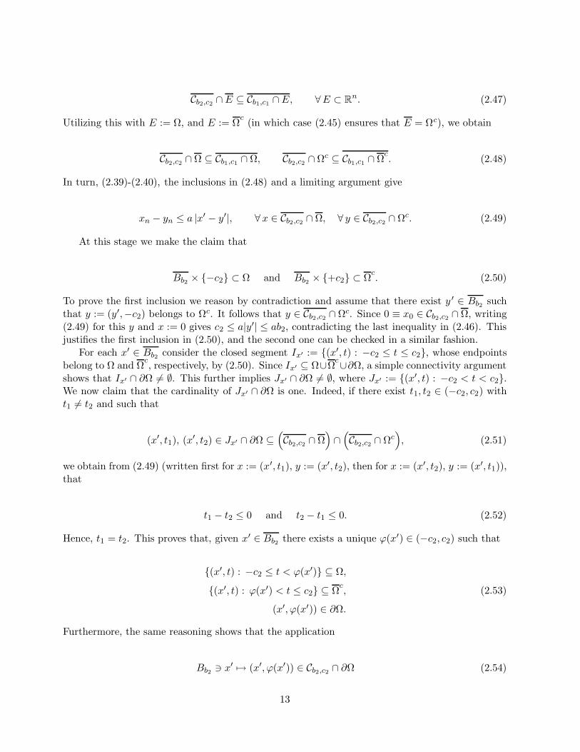
Cb2,c2 ∩E ⊆ Cb1,c1 ∩E, ∀E ⊂ Rn. (2.47)

Utilizing this with E := Ω, and E := Ωc

(in which case (2.45) ensures that E = Ωc), we obtain

Cb2,c2 ∩ Ω ⊆ Cb1,c1 ∩ Ω, Cb2,c2 ∩ Ωc ⊆ Cb1,c1 ∩ Ωc. (2.48)

In turn, (2.39)-(2.40), the inclusions in (2.48) and a limiting argument give

xn − yn ≤ a |x′ − y′|, ∀x ∈ Cb2,c2 ∩ Ω, ∀ y ∈ Cb2,c2 ∩ Ωc. (2.49)

At this stage we make the claim that

Bb2 × −c2 ⊂ Ω and Bb2 × +c2 ⊂ Ωc. (2.50)

To prove the first inclusion we reason by contradiction and assume that there exist y ′ ∈ Bb2 suchthat y := (y′,−c2) belongs to Ωc. It follows that y ∈ Cb2,c2 ∩ Ωc. Since 0 ≡ x0 ∈ Cb2,c2 ∩ Ω, writing(2.49) for this y and x := 0 gives c2 ≤ a|y′| ≤ ab2, contradicting the last inequality in (2.46). Thisjustifies the first inclusion in (2.50), and the second one can be checked in a similar fashion.

For each x′ ∈ Bb2 consider the closed segment Ix′ := (x′, t) : −c2 ≤ t ≤ c2, whose endpointsbelong to Ω and Ω

c, respectively, by (2.50). Since Ix′ ⊆ Ω∪Ω

c∪∂Ω, a simple connectivity argumentshows that Ix′ ∩ ∂Ω 6= ∅. This further implies Jx′ ∩ ∂Ω 6= ∅, where Jx′ := (x′, t) : −c2 < t < c2.We now claim that the cardinality of Jx′ ∩ ∂Ω is one. Indeed, if there exist t1, t2 ∈ (−c2, c2) witht1 6= t2 and such that

(x′, t1), (x′, t2) ∈ Jx′ ∩ ∂Ω ⊆(Cb2,c2 ∩ Ω

)∩(Cb2,c2 ∩ Ωc

), (2.51)

we obtain from (2.49) (written first for x := (x′, t1), y := (x′, t2), then for x := (x′, t2), y := (x′, t1)),that

t1 − t2 ≤ 0 and t2 − t1 ≤ 0. (2.52)

Hence, t1 = t2. This proves that, given x′ ∈ Bb2 there exists a unique ϕ(x′) ∈ (−c2, c2) such that

(x′, t) : −c2 ≤ t < ϕ(x′) ⊆ Ω,

(x′, t) : ϕ(x′) < t ≤ c2 ⊆ Ωc,

(x′, ϕ(x′)) ∈ ∂Ω.

(2.53)

Furthermore, the same reasoning shows that the application

Bb2 3 x′ 7→ (x′, ϕ(x′)) ∈ Cb2,c2 ∩ ∂Ω (2.54)

13

is onto and, since x0 ≡ 0, we also have ϕ(0) = 0. Furthermore, from (2.49) we obtain

x′, y′ ∈ Bb2 =⇒ |ϕ(x′) − ϕ(y′)| ≤ a |x′ − y′|, (2.55)

so ϕ is Lipschitz with Lipschitz constant ≤ a. From (2.53)-(2.54) it is then easy to deduce that

Cb2,c2 ∩ Ω = (x′, t) ∈ Cb2,c2 : t < ϕ(x′),Cb2,c2 ∩ Ω

c= (x′, t) ∈ Cb2,c2 : t > ϕ(x′),

Cb2,c2 ∩ ∂Ω = (x′, t) ∈ Cb2,c2 : t = ϕ(x′).(2.56)

To fully match the demands stipulated in Definition 2.2, there remains to extend ϕ : Bb2 → R

to a Lipschitz function ϕ : Rn−1 → R. That this is possible is well-known. Indeed, Kirszbraun’sTheorem asserts that any Lipschitz function defined on a subset of a metric space can be extendedto a Lipschitz function on the entire space with the same Lipschitz constant (see, e.g., [25]; for amore elementary result which will, nonetheless, do in the current context see Theorem 5.1 on p. 29in [23]). This shows that Ω is a strongly Lipschitz domain near x0, hence concluding the proof ofthe theorem.

Remarks. (i) If Ω has compact boundary, then the Lipschitz character of Ω is controlled in termsof the transversality constant of a continuous globally transversal unit vector X (hence, ultimately,on the constant a appearing in (2.33)), along with the modulus of continuity of X.

(ii) An inspection of the above proof reveals that, as a bonus feature, the following result holds:if Ω is a nonempty, proper open subset of Rn, of locally finite perimeter, for which (2.22) holds,and if X is a continuous transversal vector field near x0 ∈ ∂Ω, then ∂Ω is a Lipschitz graph nearx0 in the direction of −X(x0). As a consequence (whose significance will become clearer later), foreach t ∈ (0, to) and x ∈ ∂Ω we have

x− tX(x) ∈ Ω, x+ tX(x) ∈ Rn \ Ω, (2.57)

whenever Ω is a bounded strongly Lipschitz domain, X is a continuous globally transversal vectorfield to ∂Ω and to > 0 is sufficiently small (depending on Ω and X).

An immediate consequence of Proposition 2.2 and Theorem 2.3 is the following.

Corollary 2.6. Assume that Ω ⊂ Rn is a bounded open set of finite perimeter for which (2.22)holds. Then Ω is a strongly Lipschitz domain if and only if

inf ‖ν − f‖L∞(∂Ω,dσ) : f ∈ C0(∂Ω,Rn), |f | = 1 on ∂Ω <√

2. (2.58)

Another characterization of locally strongly Lipschitz domains can be given in terms of localcontainment of the unit normal in a fixed cone.

Corollary 2.7. Let Ω be a proper open subset of Rn, of locally finite perimeter and for which (2.22)holds. Denote by ν and σ the outward unit normal and surface measure on ∂Ω. Then Ω is a locallystrongly Lipschitz domain if and only if

∀x ∈ ∂Ω, ∃ r > 0 and ∃Γ circular cone, with vertex at 0, of aperture < π

with the property that ν(y) ∈ Γ for σ-almost every y ∈ B(x, r) ∩ ∂Ω.(2.59)

14

Proof. In one direction, if Ω is a locally strongly Lipschitz domain, then (2.59) is readily seen from(2.23). In the opposite direction, assume that (2.59) holds. Then, if v is the unit vector along thevertical axis in Γ, it follows that X ≡ v is a continuous vector field which is transversal to ∂Ω nearx. Thus, Theorem 2.3 applies and gives that Ω is a locally strongly Lipschitz domain.

We say that Ω ⊂ Rn satisfies the interior corkscrew condition if there are constants M > 1 andR > 0 such that for each x ∈ ∂Ω and r ∈ (0, R) there exists y = y(x, r) ∈ Ω, called corkscrew pointrelative to x, such that |x − y| < r and dist(y, ∂Ω) > M−1r. Also, Ω ⊂ Rn satisfies the exteriorcorkscrew condition if Ωc := Rn \Ω satisfy the interior corkscrew condition. Finally, Ω satisfies thetwo sided corkscrew condition if it satisfies both the interior and exterior corkscrew conditions.

It is clear from (2.9) and the above definition that, for an open set Ω ⊂ Rn,

Ω satisfies the two sided corkscrew condition =⇒ ∂∗Ω = ∂Ω. (2.60)

We complement this with the following elementary topological result:

Ω satisfies the exterior corkscrew condition =⇒ ∂Ω = ∂Ω. (2.61)

See Lemma 5.6 for a proof.One of the virtues of the corollary below is that it makes it clear that a bounded NTA domain

(cf. §5 for a definition) of finite perimeter is a strongly Lipschitz domain if and only if has acontinuous, globally transversal vector field.

Corollary 2.8. For each nonempty, bounded open subset Ω of Rn, the following are equivalent:

(i) Ω is a strongly Lipschitz domain;

(ii) Ω is a domain of finite perimeter, satisfying an exterior corkscrew condition, and having acontinuous globally transversal vector field.

Proof. The implication (i) ⇒ (ii) is well-known. In the opposite direction, it follows from (2.61)that the hypotheses of Theorem 2.3 are satisfied. The desired conclusion follows.

Our next results establishes a link between the cone property and the direction of the unitnormal.

Proposition 2.9. Let Ω be a proper, nonempty open subset of Rn, of locally finite perimeter. Fixx0 ∈ ∂∗Ω with the property that there exists a (circular, open, truncated, one-component) cone Γwith vertex at 0 and having aperture θ ∈ (0, π), for which

x0 + Γ ⊆ Ω. (2.62)

Denote by Γ∗ the (circular, open, infinite, one-component) cone with vertex at 0, of aperture π− θ,having the same axis as Γ and pointing in the opposite direction to Γ. Then, if ν denotes theoutward unit normal to ∂Ω, there holds

ν(x0) ∈ Γ∗. (2.63)

15

Proof. Consider the half-space

H(x0) := y ∈ Rn : ν(x0) · (y − x0) < 0 (2.64)

and, for each r > 0 and E ⊆ Rn, set

Er := y ∈ Rn : r(y − x0) + x0 ∈ E. (2.65)

Also, denote by Γ the (circular, open, infinite) cone which coincides with Γ near its vertex. Thetheorem concerning the blow-up of the reduced boundary of a set of locally finite perimeter (cf.,e.g., p. 199 in [7]) gives that

1Ωr −→ 1H(x0) in L1loc(R

n), as r → 0+. (2.66)

On the other hand, it is clear that (x0 + Γ)r ⊂ Ωr and 1(x0+Γ)r−→ 1x0+eΓ in L1

loc(Rn) as r → 0+.

This and (2.65) then allow us to write

1x0+eΓ = limr→0+

1(x0+Γ)r= lim

r→0+

(1(x0+Γ)r

· 1Ωr

)

=(

limr→0+

1(x0+Γ)r

)·(

limr→0+

1Ωr

)= 1x0+eΓ · 1H(x0)

= 1(x0+eΓ)∩H(x0), (2.67)

in a pointwise a.e. sense in Rn. In turn, this implies

x0 + Γ ⊆ H(x0). (2.68)

Now, (2.63) readily follows from this, (2.64), the definition of Γ∗ and simple geometrical consider-ations.

Corollary 2.10. Assume that Ω is a proper, nonempty open subset of Rn, of locally finite perimeter,and for which (2.22) holds. Denote by σ the surface measure on ∂Ω.

Then Ω is a locally strongly Lipschitz domain if and only if the following condition is verified.For every x ∈ ∂Ω there exist r > 0 along with a (circular, open, truncated, one-component) cone Γwith vertex at 0 ∈ Rn such that

y + Γ ⊆ Ω for σ-a.e. y ∈ B(x, r) ∩ ∂Ω. (2.69)

Proof. In one direction, it is clear that if Ω ⊂ Rn is a locally strongly Lipschitz domain then Ωsatisfies (2.69). Consider next the opposite implication, which is the crux of the matter here. Fixan arbitrary point x ∈ ∂Ω, and let r > 0, Γ be such that (2.69) holds. One can, of course, assumethat the aperture of Γ is < π. In concert with the fact that σ is supported on ∂ ∗Ω, condition (2.69)implies y + Γ ⊆ Ω for σ-a.e. y ∈ B(x, r) ∩ ∂∗Ω. In light of Proposition 2.9, this further entailsν(y) ∈ Γ∗ for σ-a.e. y ∈ B(x, r) ∩ ∂Ω, where ν stands for the outward unit normal to ∂Ω. Thenthe desired conclusion follows from Corollary 2.7.

16

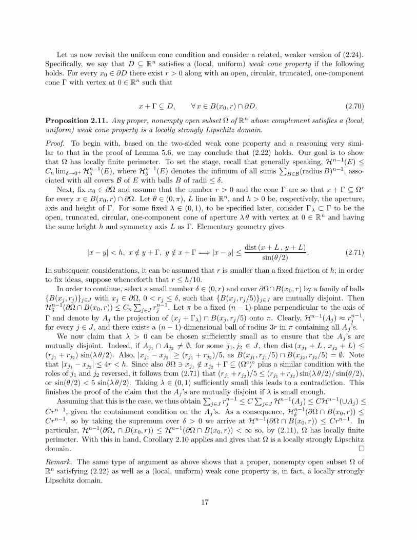
Let us now revisit the uniform cone condition and consider a related, weaker version of (2.24).Specifically, we say that D ⊆ Rn satisfies a (local, uniform) weak cone property if the followingholds. For every x0 ∈ ∂D there exist r > 0 along with an open, circular, truncated, one-componentcone Γ with vertex at 0 ∈ Rn such that

x+ Γ ⊆ D, ∀x ∈ B(x0, r) ∩ ∂D. (2.70)

Proposition 2.11. Any proper, nonempty open subset Ω of Rn whose complement satisfies a (local,uniform) weak cone property is a locally strongly Lipschitz domain.

Proof. To begin with, based on the two-sided weak cone property and a reasoning very simi-lar to that in the proof of Lemma 5.6, we may conclude that (2.22) holds. Our goal is to showthat Ω has locally finite perimeter. To set the stage, recall that generally speaking, Hn−1(E) ≤Cn limδ→0+ Hn−1

δ (E), where Hn−1δ (E) denotes the infimum of all sums

∑B∈B(radiusB)n−1, asso-

ciated with all covers B of E with balls B of radii ≤ δ.Next, fix x0 ∈ ∂Ω and assume that the number r > 0 and the cone Γ are so that x + Γ ⊆ Ωc

for every x ∈ B(x0, r) ∩ ∂Ω. Let θ ∈ (0, π), L line in Rn, and h > 0 be, respectively, the aperture,axis and height of Γ. For some fixed λ ∈ (0, 1), to be specified later, consider Γλ ⊂ Γ to be theopen, truncated, circular, one-component cone of aperture λ θ with vertex at 0 ∈ Rn and havingthe same height h and symmetry axis L as Γ. Elementary geometry gives

|x− y| < h, x /∈ y + Γ, y /∈ x+ Γ =⇒ |x− y| ≤ dist (x+ L , y + L)

sin(θ/2). (2.71)

In subsequent considerations, it can be assumed that r is smaller than a fixed fraction of h; in orderto fix ideas, suppose whenceforth that r ≤ h/10.

In order to continue, select a small number δ ∈ (0, r) and cover ∂Ω∩B(x0, r) by a family of ballsB(xj , rj)j∈J with xj ∈ ∂Ω, 0 < rj ≤ δ, such that B(xj , rj/5)j∈J are mutually disjoint. ThenHn−1

δ (∂Ω ∩B(x0, r)) ≤ Cn∑

j∈J rn−1j . Let π be a fixed (n− 1)-plane perpendicular to the axis of

Γ and denote by Aj the projection of (xj + Γλ) ∩ B(xj, rj/5) onto π. Clearly, Hn−1(Aj) ≈ rn−1j ,

for every j ∈ J , and there exists a (n− 1)-dimensional ball of radius 3r in π containing all Aj ’s.We now claim that λ > 0 can be chosen sufficiently small as to ensure that the Aj ’s are

mutually disjoint. Indeed, if Aj1 ∩ Aj2 6= ∅, for some j1, j2 ∈ J , then dist (xj1 + L , xj2 + L) ≤(rj1 + rj2) sin(λ θ/2). Also, |xj1 − xj2 | ≥ (rj1 + rj2)/5, as B(xj1 , rj1/5) ∩ B(xj2 , rj2/5) = ∅. Notethat |xj1 − xj2 | ≤ 4r < h. Since also ∂Ω 3 xj1 /∈ xj2 + Γ ⊆ (Ωc) plus a similar condition with theroles of j1 and j2 reversed, it follows from (2.71) that (rj1 + rj2)/5 ≤ (rj1 + rj2) sin(λ θ/2)/ sin(θ/2),or sin(θ/2) < 5 sin(λ θ/2). Taking λ ∈ (0, 1) sufficiently small this leads to a contradiction. Thisfinishes the proof of the claim that the Aj ’s are mutually disjoint if λ is small enough.

Assuming that this is the case, we thus obtain∑

j∈J rn−1j ≤ C

∑j∈J Hn−1(Aj) ≤ CHn−1(∪Aj) ≤

Crn−1, given the containment condition on the Aj’s. As a consequence, Hn−1δ (∂Ω ∩ B(x0, r)) ≤

Crn−1, so by taking the supremum over δ > 0 we arrive at Hn−1(∂Ω ∩ B(x0, r)) ≤ Crn−1. Inparticular, Hn−1(∂Ω∗ ∩ B(x0, r)) ≤ Hn−1(∂Ω ∩ B(x0, r)) < ∞ so, by (2.11), Ω has locally finiteperimeter. With this in hand, Corollary 2.10 applies and gives that Ω is a locally strongly Lipschitzdomain.

Remark. The same type of argument as above shows that a proper, nonempty open subset Ω ofRn satisfying (2.22) as well as a (local, uniform) weak cone property is, in fact, a locally stronglyLipschitz domain.

17

Definition 2.3. A nonempty, bounded open subset Ω of Rn is called a bounded C1-domain if it isa strongly Lipschitz domain and the Lipschitz functions ϕ : Rn−1 → R whose graphs locally describe∂Ω, in the sense of Definition 2.2, can be taken to be of class C 1.

We conclude this section with an intrinsic characterization of the class of bounded C 1 domainsin Rn. Specifically, we shall prove the following.

Theorem 2.12. Assume that Ω is a nonempty, bounded open subset of Rn, of locally finite perime-ter, for which (2.22) holds, and denote by ν the geometric measure theoretic outward unit normalto ∂Ω, as defined in (2.2)-(2.3). Then Ω is a C1 domain if and only if, after altering ν on a set ofσ-measure zero,

ν ∈ C0(∂Ω,Rn). (2.72)

Proof. In one direction, assume that Ω is a bounded C 1 domain, and fix x0 ∈ ∂Ω. If ϕ : Rn−1 → R

is a function of class C1 whose graph, in a suitable system of coordinates, (x′, t), isometric to thestandard one, matches ∂Ω near x0, then (2.23) holds. Then (2.72) can be read off this.

The main issue here is the opposite implication. Assuming that (2.72) holds, it follows that νis a continuous globally transversal vector field to Ω. Theorem 2.3 then gives that Ω is a stronglyLipschitz domain. Then, if the point x0 ∈ ∂Ω (identified with 0 ∈ Rn) and the Lipschitz functionϕ : Rn−1 → R are as in Definition 2.2, it follows from (2.23) that νn(x′, ϕ(x′)) 6= 0 and

∂jϕ(x′) = − νj(x′, ϕ(x′))

νn(x′, ϕ(x′)), j = 1, ..., n− 1, (2.73)

granted that x′ is near 0 ∈ Rn−1. Since ϕ is continuous and (2.72) holds, this further implies thatall first order partial derivatives of ϕ are continuous functions near 0 ∈ Rn−1. With this in hand,it is then easy to conclude that Ω is, in fact, a C 1 domain.

In closing, we wish to point out that, under the same hypotheses as Theorem 2.12, the argumentin the proof above shows that that, in fact,

Ω is a C1+α-domain ⇐⇒ ν ∈ Cα(∂Ω,Rn), (2.74)

for every α ∈ (0, 1), and

Ω is a C1,1-domain ⇐⇒ ν is Lipschitz. (2.75)

3 Finite perimeter domains under bi-Lipschitz and C1 diffeomor-

phisms

As is well-known, the class of topological boundaries is invariant under topological homeomor-phisms. Our first result clarifies how the measure theoretic boundaries reduced boundaries of setsof locally finite perimeter in Rn transform under bi-Lipschitz maps. Before stating it, we take careof a number of prerequisites.

If O ⊆ Rn and F : O → Rn is a Lipschitz function, set

18

Lip (F,O) := sup|F (x) − F (y)|/|x− y| : x, y ∈ O, x 6= y

. (3.1)

Then, with Hs denoting the s-dimensional Hausdorff measure in Rn, we have (cf. Theorem 1 onp. 75 in [7])

Hs(F (E)) ≤ [Lip (F,O)]s Hs(E), ∀E ⊂ O, s ≥ 0. (3.2)

As is well-known, if O ⊆ Rn is open and F = (F1, ..., Fn) : O → Rn is a Lipschitz function then theJacobian matrix of F , i.e., DF := (∂kFj)1≤j,k≤n, exists a.e. (cf. [21]) and

‖DF‖ ≤ Lip (F,O) a.e. in O, (3.3)

where, given a matrix A, ‖A‖ denotes the norm of A viewed as a linear operator. Recall that forany n×n matrix A, |detA| is the volume of the parallelopiped spanned by the vectors Ae1, ..., Aen,so |detA| ≤ ‖Ae1‖ · · · ‖Aen‖ ≤ ‖A‖n. Consequently,

|detDF (x)| ≤ [Lip (F,O)]n for a.e. x ∈ O. (3.4)

Going further, call a Lipschitz function F : O → Rn bi-Lipschitz if F is one-to-one andLip (F−1, F (O)) < ∞. It is know that bi-Lipschitz functions are open; in particular, F (O) isopen and F : O → F (O) is a topological homeomorphism. Furthermore, while the Chain Rulemay, generally speaking, fail for Lipschitz functions, we do have (with In×n denoting the n × nidentity matrix),

[(DF−1) F ][DF ] = In×n, a.e. in O, (3.5)

if O ⊆ Rn is open and F : O → Rn is bi-Lipschitz. Hence, in this case we also have the lower bound

[Lip (F−1, F (O))]−n ≤ |detDF (x)| for a.e. x ∈ O. (3.6)

In addition, as observed by H.Rademacher (cf. p. 354 in [21]),

O connected =⇒ either det (DF ) > 0 a.e. in O, or det (DF ) < 0 a.e. in O. (3.7)

In the sequel, whenever the context is clear, we shall lighten the notation and simply write Lip (F ),Lip (F−1) in place of Lip (F,O), Lip (F−1, F (O)). A case in point is the statement that if thefunction F : O → Rn is bi-Lipschitz then, for every x ∈ O and r > 0,

B(F (x), (LipF−1)−1r) ∩ F (O) ⊆ F (B(x, r) ∩ O) ⊆ B(F (x), (LipF ) r) ∩ F (O). (3.8)

Call F : O → Rn locally Lipschitz (respectively, locally bi-Lipschitz) if for every x ∈ O there existsr > 0 with the property that F : B(x, r) ∩ O → Rn is Lipschitz (respectively, bi-Lipschitz).

19

Next, we briefly review the concept of the push-forward of a measure. Let O, O ⊆ Rn be twoopen sets and let F : O → O be a continuous, proper map. If µ is a Borelian measure on O wedefine the Borelian measure F∗µ on O, the push-forward of µ via F , as

F∗µ(E) := µ(F−1(E)), ∀E ⊆ O Borel set. (3.9)

Note that this entails

∫f dF∗µ =

∫f F dµ, ∀ f ∈ C0(O), compactly supported, (3.10)

(F∗µ)bE = F∗(µbF−1(E)), ∀E ⊆ O Borel set, (3.11)

F∗(fµ) = (f F−1)F∗µ if F is a topological homeomorphism, (3.12)

G∗(F∗µ) = (G F )∗µ, if G : O → ˜O is a continuous, proper function. (3.13)

Finally, we make the following definition. Given a Radon measure µ in Rn and two sets A,B ⊆Rn, we write A ≡ B modulo µ, if µ(A4B) = 0, where A4B := (A\B)∪ (B \A) is the symmetricdifference of A and B.

Proposition 3.1. Let Ω ⊂ Rn be an open set of locally finite perimeter, O an open neighborhoodof Ω, and F : O → Rn an injective, locally bi-Lipschitz mapping. Then Ω := F (Ω) is also an openset of locally finite perimeter and, in addition,

∂∗Ω = F (∂∗Ω). (3.14)

Moreover,

∂∗Ω ≡ F (∂∗Ω) modulo Hn−1, (3.15)

so that, in particular,

σ(Rn \ F (∂∗Ω)) = 0, (3.16)

where σ denotes the surface measure on ∂Ω.Finally, if σ stands for the surface measure on ∂Ω, then

σ and F∗σ are mutually absolutely continuous. (3.17)

Proof. Formula (3.14) is a consequence of definition (2.9) and the fact that an injective bi-Lipschitzmapping is a topological homeomorphism that changes the Lebesgue measure of the subsets of agiven compact set at most by a factor (that is bounded and bounded away from zero – cf. (3.2)).Then the fact that Ω has locally finite perimeter is a consequence of (3.14), (3.2) and (2.10).

Turning our attention to (3.15), using (2.8), (3.14) and (3.2), we compute

20

Hn−1(∂∗Ω \ F (∂∗Ω)) = Hn−1(∂∗Ω \ F (∂∗Ω))

= Hn−1(F (∂∗Ω) \ F (∂∗Ω)) ≤ Hn−1(F (∂∗Ω \ ∂∗Ω)) = 0, (3.18)

since Hn−1(∂∗Ω \ ∂∗Ω) = 0 and the class of sets of Hn−1-measure zero is invariant under locallybi-Lipschitz mappings. Also,

Hn−1(F (∂∗Ω) \ ∂∗Ω) = Hn−1(F (∂∗Ω) \ ∂∗Ω)

= Hn−1(F (∂∗Ω) \ F (∂∗Ω)) = Hn−1(∅) = 0. (3.19)

In concert, (3.18)-(3.19) give that ∂∗Ω ≡ F (∂∗Ω) modulo Hn−1. With this in hand, (3.16) followsfrom (2.7).

Finally, E ⊆ ∂Ω is σ-measurable if and only if F−1(E) is σ-measurable and, granted what wehave proved up to this point,

(F∗σ)(E) = 0 ⇔ σ(F−1(E)) = 0 ⇔ Hn−1(∂∗Ω \ F−1(E)) = 0

⇔ Hn−1(∂∗Ω \ F−1(E)) = 0 ⇔ Hn−1(F−1(∂∗Ω) \ F−1(E)) = 0

⇔ Hn−1(F−1(∂∗Ω \ E)) = 0 ⇔ Hn−1(∂∗Ω \E) = 0

⇔ Hn−1(∂∗Ω \ E) = 0 ⇔ σ(E) = 0. (3.20)

This gives (3.17), completing the proof of the proposition.

In the context of Proposition 3.1, (3.17) raises the issue of computing the Radon-Nikodymderivatives dσ/dF∗σ and d(F−1)∗σ/dσ. Our next two theorems are devoted to addressing thisissue. To state the first, we need to introduce some more notation. Given a n×n matrix A, denoteby A> the transposed of A, and by adjA the adjunct matrix (sometimes denoted Cof(A), whoseentries are the cofactors of A). In particular,

A>(adjA) = (adjA)A> = (detA) In×n. (3.21)

We also let trA denote the trace of the n× n matrix A, and equip the space of such matrices withthe inner product 〈A,B〉 := tr(A>B). Finally, if A = (ajk)1≤j,k≤n is a matrix with variable entries,we set

DivA := (∂kajk)1≤j≤n, (3.22)

i.e., DivA is the vector whose components are the divergences of the lines of the matrix A.

Theorem 3.2. Let Ω ⊂ Rn be a domain of locally finite perimeter, O an open neighborhood of Ω,and let F : O → Rn be an orientation preserving C1-diffeomorphism.

Then Ω := F (Ω) is a domain of locally finite perimeter and if ν, ν and σ, σ are, respectively, theoutward unit normals and surface measures on ∂Ω and ∂Ω, then

21

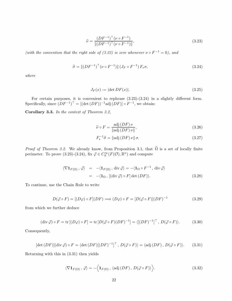
ν =(DF−1)>(ν F−1)

‖(DF−1)>(ν F−1)‖ , (3.23)

(with the convention that the right side of (3.23) is zero whenever ν F −1 = 0), and

σ = ‖(DF−1)>(ν F−1)‖ (JF F−1)F∗σ, (3.24)

where

JF (x) := |detDF (x)|. (3.25)

For certain purposes, it is convenient to rephrase (3.23)-(3.24) in a slightly different form.Specifically, since (DF−1)> = [(det (DF ))−1adj (DF )] F−1, we obtain:

Corollary 3.3. In the context of Theorem 3.2,

ν F =adj (DF ) ν

‖adj (DF ) ν‖ , (3.26)

F−1∗ σ = ‖adj (DF ) ν‖σ. (3.27)

Proof of Theorem 3.2. We already know, from Proposition 3.1, that Ω is a set of locally finiteperimeter. To prove (3.23)-(3.24), fix ~ϕ ∈ C∞

0 (F (O),Rn) and compute

〈∇1F (Ω) , ~ϕ〉 = −〈1F (Ω) , div ~ϕ〉 = −〈1Ω F−1 , div ~ϕ〉= −〈1Ω , [(div ~ϕ) F ] det (DF )〉. (3.28)

To continue, use the Chain Rule to write

D(~ϕ F ) = [(Dϕ) F ](DF ) =⇒ (Dϕ) F = [D(~ϕ F )](DF )−1 (3.29)

from which we further deduce

(div ~ϕ) F = tr [(Dϕ) F ] = tr [D(~ϕ F )(DF )−1] = 〈[(DF )−1]> , D(~ϕ F )〉. (3.30)

Consequently,

[det (DF )](div ~ϕ) F = 〈det (DF )[(DF )−1]> , D(~ϕ F )〉 = 〈adj (DF ) , D(~ϕ F )〉. (3.31)

Returning with this in (3.31) then yields

〈∇1F (Ω) , ~ϕ〉 = −⟨1F (Ω) , 〈adj (DF ) , D(~ϕ F )〉

⟩. (3.32)

22

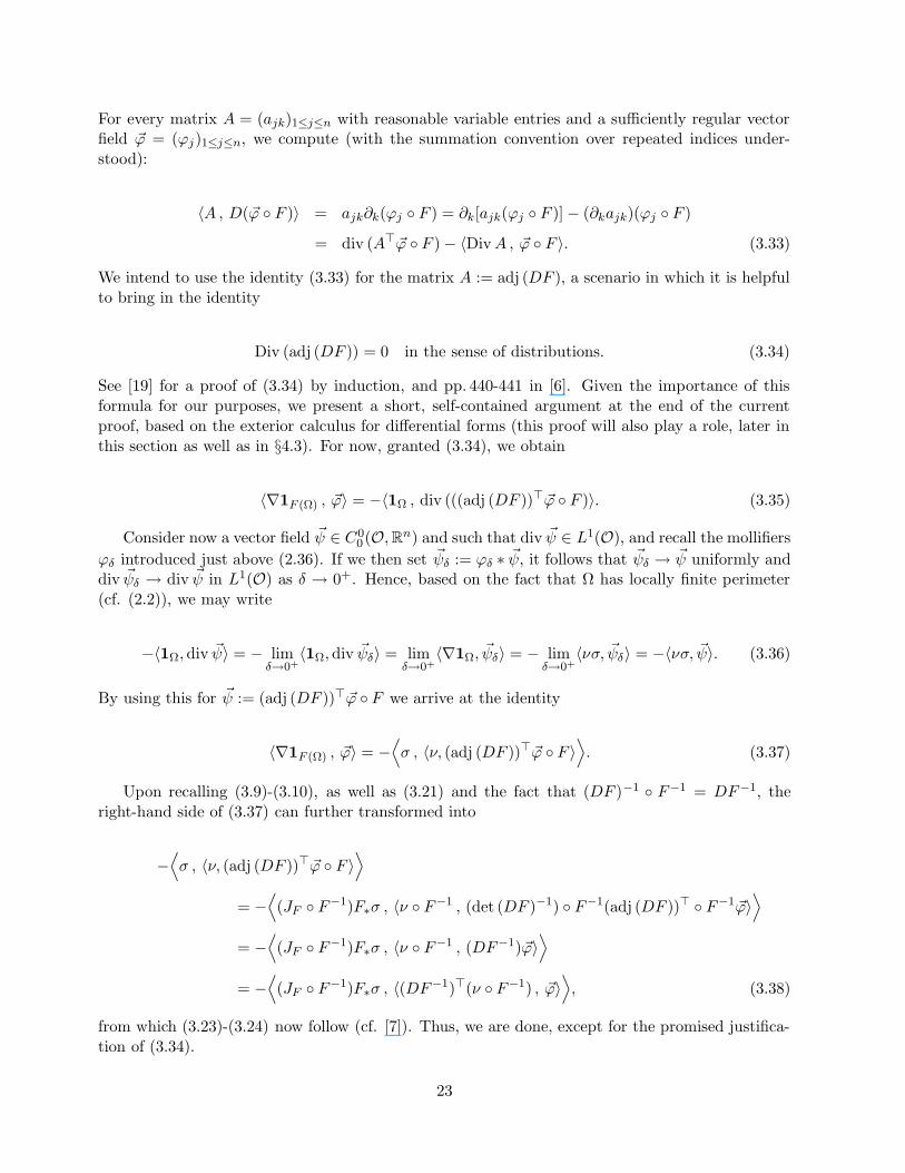
For every matrix A = (ajk)1≤j≤n with reasonable variable entries and a sufficiently regular vectorfield ~ϕ = (ϕj)1≤j≤n, we compute (with the summation convention over repeated indices under-stood):

〈A , D(~ϕ F )〉 = ajk∂k(ϕj F ) = ∂k[ajk(ϕj F )] − (∂kajk)(ϕj F )

= div (A>~ϕ F ) − 〈DivA , ~ϕ F 〉. (3.33)

We intend to use the identity (3.33) for the matrix A := adj (DF ), a scenario in which it is helpfulto bring in the identity

Div (adj (DF )) = 0 in the sense of distributions. (3.34)

See [19] for a proof of (3.34) by induction, and pp. 440-441 in [6]. Given the importance of thisformula for our purposes, we present a short, self-contained argument at the end of the currentproof, based on the exterior calculus for differential forms (this proof will also play a role, later inthis section as well as in §4.3). For now, granted (3.34), we obtain

〈∇1F (Ω) , ~ϕ〉 = −〈1Ω , div (((adj (DF ))>~ϕ F )〉. (3.35)

Consider now a vector field ~ψ ∈ C00 (O,Rn) and such that div ~ψ ∈ L1(O), and recall the mollifiers

ϕδ introduced just above (2.36). If we then set ~ψδ := ϕδ ∗ ~ψ, it follows that ~ψδ → ~ψ uniformly anddiv ~ψδ → div ~ψ in L1(O) as δ → 0+. Hence, based on the fact that Ω has locally finite perimeter(cf. (2.2)), we may write

−〈1Ω,div ~ψ〉 = − limδ→0+

〈1Ω,div ~ψδ〉 = limδ→0+

〈∇1Ω, ~ψδ〉 = − limδ→0+

〈νσ, ~ψδ〉 = −〈νσ, ~ψ〉. (3.36)

By using this for ~ψ := (adj (DF ))>~ϕ F we arrive at the identity

〈∇1F (Ω) , ~ϕ〉 = −⟨σ , 〈ν, (adj (DF ))>~ϕ F 〉

⟩. (3.37)

Upon recalling (3.9)-(3.10), as well as (3.21) and the fact that (DF )−1 F−1 = DF−1, theright-hand side of (3.37) can further transformed into

−⟨σ , 〈ν, (adj (DF ))>~ϕ F 〉

⟩

= −⟨(JF F−1)F∗σ , 〈ν F−1 , (det (DF )−1) F−1(adj (DF ))> F−1~ϕ〉

⟩

= −⟨(JF F−1)F∗σ , 〈ν F−1 , (DF−1)~ϕ〉

⟩

= −⟨(JF F−1)F∗σ , 〈(DF−1)>(ν F−1) , ~ϕ〉

⟩, (3.38)

from which (3.23)-(3.24) now follow (cf. [7]). Thus, we are done, except for the promised justifica-tion of (3.34).

23

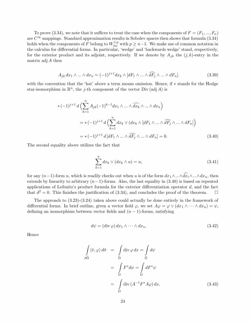
To prove (3.34), we note that it suffices to treat the case when the components of F = (F1, ..., Fn)are C∞ mappings. Standard approximation results in Sobolev spaces then shows that formula (3.34)holds when the components of F belong to W 1,p

loc with p ≥ n−1. We make use of common notation inthe calculus for differential forms. In particular, ‘wedge’ and ‘backwards wedge’ stand, respectively,for the exterior product and its adjoint, respectively. If we denote by Ajk the (j, k)-entry in thematrix adjA then

Ajk dx1 ∧ ... ∧ dxn = (−1)j+1dxk ∧ [dF1 ∧ ... ∧ dFj ∧ ... ∧ dFn]. (3.39)

with the convention that the ‘hat’ above a term means omission. Hence, if ∗ stands for the Hodgestar-isomorphism in Rn, the j-th component of the vector Div (adjA) is

∗ (−1)j+1 d( n∑

k=1

Ajk(−1)k−1dx1 ∧ ... ∧ dxk ∧ ... ∧ dxn

)

= ∗ (−1)j+1 d( n∑

k=1

dxk ∨ (dxk ∧ [dF1 ∧ ... ∧ dFj ∧ ... ∧ dFn])

= ∗ (−1)j+1 d [dF1 ∧ ... ∧ dFj ∧ ... ∧ dFn] = 0. (3.40)

The second equality above utilizes the fact that

n∑

k=1

dxk ∨ (dxk ∧ u) = u, (3.41)

for any (n−1)-form u, which is readily checks out when u is of the form dx1∧...∧ dxi∧...∧dxn, thenextends by linearity to arbitrary (n−1)-forms. Also, the last equality in (3.40) is based on repeatedapplications of Leibnitz’s product formula for the exterior differentiation operator d, and the factthat d2 = 0. This finishes the justification of (3.34), and concludes the proof of the theorem.

The approach to (3.23)-(3.24) taken above could actually be done entirely in the framework ofdifferential forms. In brief outline, given a vector field ϕ, we set Aϕ = ϕ ∨ (dx1 ∧ · · · ∧ dxn) = ψ,defining an isomorphism between vector fields and (n− 1)-forms, satisfying

dψ = (divϕ) dx1 ∧ · · · ∧ dxn. (3.42)

Hence

∫

∂ eΩ

〈ν, ϕ〉 dσ =

∫

eΩ

divϕdx =

∫

eΩ

dψ

=

∫

Ω

F ∗dψ =

∫

Ω

dF ∗ψ

=

∫

Ω

div (A−1F ∗Aϕ) dx, (3.43)

24

the last identity by (3.42). If T : Rn → Rn is a linear mapping, let ΛkT denote the k-fold exteriorproduct of T with itself. Then, parallel to the first identity in (3.43), the last quantity in (3.43) isequal to

∫∂Ω〈ν , A−1Λn−1DF (x)>Aϕ(F (x))〉 dσ, and we obtain

ν(y) σ =(A−1Λn−1DF (F−1(y))>A

)>ν(F−1(y))F∗σ. (3.44)

Obtaining the equivalence of (3.44) with (3.23)–(3.24) is then a piece of algebra related to Cramer’sformula. We omit the details.

In the approach via (3.43), the role of the somewhat mysterious formula (3.34) is taken by themore familiar identity

d(F ∗ψ) = F ∗(dψ), (3.45)

where ψ is a differential form (in the current context, an (n− 1)-form).It is of interest to present an alternative analysis of the behavior of finite perimeter domains

under C1-diffeomorphisms which avoids the use of identities involving the divergence of vectorfields. Here we do that and develop a line of proof which, instead, uses mollifiers, the change ofvariable formula for continuous integrands, and a limiting argument.

Specifically, let Ω ⊂ Rn be a bounded open set of finite perimeter, and let F be a C 1 diffeomor-phism of a neighborhood O of Ω onto O ⊂ Rn, mapping Ω to Ω. We will show that Ω has finiteperimeter and give a formula for νσ = −∇1eΩ in terms of νσ = −∇1Ω.

To begin, let ϕδ be a mollifier, with (small) compact support, set χδ = ϕδ ∗ 1Ω, and setχδ = χδ F−1, so

χδ −→ 1eΩ, χδ −→ 1Ω, in L1-norm, (3.46)

as δ → 0. Hence

∇χδ −→ ∇1eΩ, ∇χδ −→ ∇1Ω, in D′(Rn). (3.47)

The chain rule gives

∇χδ(F (x))DF (x) = ∇χδ(x), and ∇χδ(y) = ∇χδ(F−1(y))DF−1(y). (3.48)

(To put DF (x) on the left, make it DF (x)>.) Since Ω is assumed to have finite perimeter, if Mdenotes the collection of Borel measures in Rn, we have

∇χδ −→ ∇1Ω, weak∗ in M, (3.49)

with a bound on ‖∇χδ‖L1 for δ ∈ (0, 1]. Hence, by (3.48), we have a bound on ‖∇χδ‖L1 . It followsfrom this and (3.47) that Ω has finite perimeter and

∇χδ −→ ∇1eΩ, weak∗ in M. (3.50)

25

That is to say, ∇1eΩ = −νσ with σ surface area on ∂Ω and

−∫

〈ν, ϕ〉 dσ = limδ→0

∫〈∇χδ(y), ϕ(y)〉 dy, (3.51)

for each ϕ ∈ C00 (O,Rn). Now, with JF (x) = |detDF (x)|, we have

∫〈∇χδ(y), ϕ(y)〉 dy =

∫〈∇χδ(F (x)), ϕ(F (x))〉JF (x) dx

=

∫〈∇χδ(x), DF (x)−1ϕ(F (x))〉JF (x) dx

→ −∫

〈ν(x), JF (x)DF (x)−1ϕ(F (x))〉 dσ(x). (3.52)

Hence, with F∗σ given as in (3.9), we have from (3.51)–(3.52) that for each ϕ ∈ C 00 (O,Rn),

∫〈ν, ϕ〉 dσ =

∫〈JF (x)(DF (x)−1)>ν(x), ϕ(F (x))〉 dσ(x)

=

∫〈JF (F−1(y))DF−1(y)>ν(F−1(y)), ϕ(y)〉 dF∗σ, (3.53)

so

ν(y) σ = DF−1(y)>ν(F−1(y)) JF (F−1(y))F∗σ, (3.54)

again giving (3.23) and (3.24).

We next seek to relate σ to F∗σ in the more general case where F is merely bi-Lipschitz. Insuch a more general setting (3.46)–(3.51) continue to hold, but the convergence result in (3.52)might fail, since DF and JF need not be continuous (and, in fact, the right side of (3.54) mightnot be well defined). In such a scenario, we shall make use of the (generalized) area formula, aspresented in § 12 of [23]. To set the stage for doing so, for the convenience of the reader we firstreview a number of definitions.

A set M ⊂ Rn is called countably (n− 1)-rectifiable if it is a countable disjoint union

M =

∞⋃

j=0

Mj (3.55)

where Hn−1(M0) = 0 and each Mj, j ≥ 1, is a compact subset of an (n−1)-dimensional C 1 surfaceNj in Rn. A countably rectifiable set M ⊂ Rn need not have tangent planes in the ordinary sense,but it will have approximate tangent planes. By definition, an (n − 1)-plane TxM ⊂ Rn passingthrough x ∈M is called the approximate tangent (n− 1)-plane to M at x provided

lim supr0

r−n Hn−1(M ∩B(x, r)

)> 0, and

lim supr0

r−n Hn−1(y ∈M ∩B(x, r) : dist (y, TxM) > λ |x− y|

)= 0, ∀λ > 0.

(3.56)

26

Note that if such an (n − 1)-plane exists, then it is unique (so the notation TxM is justified).Furthermore, the existence of an approximate tangent (n − 1)-plane Hn−1-almost everywhere is,for Hn−1-measurable sets of locally finite Hausdorff measure, equivalent to countably (n − 1)-rectifiability. See Theorem 1.5 in [8]. In the context of (3.55),

TxM = TxNj for Hn−1-a.e. x ∈ Nj , (3.57)

where TxNj is the differential geometric tangent plane to the C 1 surface Nj at x. See Remark 11.7on p. 61 in [23].

Assume next that f is a locally bi-Lipschitz, real-valued function defined in an open neigh-borhood O ⊆ Rn of M . Then Rademacher’s differentiability theorem ensures that there exists aunique locally bounded function on M , called the gradient of f relative to M , such that

∇Mf : M −→ Rn, ∇Mf(x) = ∇Njf(x) (3.58)

for Hn−1-a.e. x ∈Mj with the property that f |Njis differentiable at x. Above, ∇Nj represents the

differential geometric gradient on the C1 surface Nj . From (3.57) (cf. also Remark 12.2 on p. 67 in[23]), we then have

∇Mf(x) ∈ TxM for Hn−1-a.e. points x ∈M. (3.59)

Going further, we define the differential of f on M by

dMfx : TxM −→ R, dMfx(τ) := 〈τ,∇Mf(x)〉, τ ∈ TxM, (3.60)

at all points x ∈ M where TxM and ∇Mf(x) exist (hence, Hn−1-a.e.). If instead of being real-valued, F = (F1, ..., Fn) takes values in Rn, we define

dMFx : TxM −→ Rn, dMFx(τ) :=

n∑

i=1

〈τ,∇MFi(x)〉ei, τ ∈ TxM, (3.61)

where ei = (δik)1≤k≤n, 1 ≤ i ≤ n, are the vectors in the standard orthonormal basis in Rn. Finally,we introduce the Jacobian determinant of F on M as

JMF (x) :=√

det [(dMFx)∗ (dMFx)], (3.62)

where (dMFx)∗ : Rn → TxM is the adjoint of (3.61).In this terminology, and assuming that F is injective and locally bi-Lipschitz from some ope

neighborhood of the countably (n− 1)-rectifiable set M ⊂ Rn into Rn, the area formula proved in§ 12 of [23] reads (after correcting a typo) as follows:

Hn−1(F (E)) =

∫

EJMF dHn−1, whenever E ⊆M is Hn−1-measurable. (3.63)

According to a famous theorem of De Giorgi (cf. Theorem 14.3 on p. 72 of [23]), if Ω ⊆ Rn is an openset of locally finite perimeter then ∂∗Ω is countably (n− 1)-rectifiable, so the above considerationsapply to this set.

27

Theorem 3.4. Let Ω ⊂ Rn be a domain of locally finite perimeter, O an open neighborhood of Ω,and let F : O → Rn be an injective, locally bi-Lipschitz function. Set Ω := F (Ω) and denote by σ,σ, respectively, surface measure on ∂Ω and ∂Ω. Then

σ = [(J∂∗ΩF ) F−1]F∗σ, σ = [(J∂∗ eΩ

F−1) F ] (F−1)∗σ, (3.64)

and

(J∂∗ΩF )−1 = (J∂∗eΩF−1) F. (3.65)

Proof. To begin with, Proposition 3.1 ensures that Ω is a set of locally finite perimeter, so σ iswell-defined. To proceed, let us recast (3.63) in the form

(JMF )Hn−1bM = (F−1)∗(Hn−1bF (M)). (3.66)

We then write

(J∂∗ΩF )σ = (J∂∗ΩF )Hn−1b∂∗Ω by (2.6),

= (F−1)∗(Hn−1bF (∂∗Ω)) by (3.66) with M = ∂∗Ω,

= (F−1)∗(Hn−1b∂∗Ω) by (3.15),

= (F−1)∗ σ by (2.6) with Ω in place of Ω.

(3.67)

This and (3.12)-(3.13) in turn imply σ = F∗[(J∂∗ΩF )σ] = [(J∂∗ΩF ) F−1]F∗σ, as desired. Thenthe second formula in (3.64) is a consequence of this, reasoning with the roles of Ω, Ω reversed.Finally, (3.65) follows from the second identity in (3.64) and (3.67).

In the context of Theorem 3.2, a comparison of (3.24) and (3.64) shows that, although notobvious from definitions, formula

J∂∗ΩF = ‖[(DF−1)> F ]ν‖ |det (DF )|, if F is a C1-diffeomorphism, (3.68)

must, nonetheless, be true. It would be therefore instructive to present a direct proof of (3.68),which does not rely on Theorems 3.2-3.4. To this end, fix a point x ∈ ∂∗Ω with the property thatTx∂

∗Ω. Since F = (F1, ..., Fn) is of class C1 in a neighborhood of ∂Ω, it follows from definitionsthat for each i = 1, ..., n,

∇∂∗ΩFi = πx∇Fi, πx : Rn −→ Tx∂∗Ω orthogonal projection. (3.69)

Consequently, for each τ ∈ Tx∂∗Ω,

d∂∗ΩFx(τ) =n∑

i=1

〈τ,∇∂∗ΩFi〉ei =n∑

i=1

〈τ,∇Fi〉ei = [DF (x)]τ. (3.70)

28

To continue, abbreviate W := Tx∂∗Ω A := DF (x), A := d∂∗ΩFx. Hence, W is a (n − 1)-plane in

Rn and A : Rn → Rn, A : W → Rn, are linear mappings with the property that A = A|W . Fix anorthonormal basis τi1≤i≤n−1 in Tx∂

∗Ω. Using notation and results summarized in the appendix,we then write

J∂∗ΩF (x) =√

det (A∗A) by (3.62),

= |Aτ1 × · · · ×Aτn−1| by (5.13),

= |Aτ1 × · · · × Aτn−1| since A = A|W ,

= |detA| ‖(A−1)>(τ1 × · · · × τn−1)‖ by (5.11),

= |detA| ‖(A−1)>ν(x)‖ by (5.7),

= |det (DF )(x)| ‖[(DF (x))−1 ]>ν(x)‖ by the definition of A,= |det (DF )(x)| ‖[(DF−1)F (x)]>ν(x)‖ since (DF )−1 = (DF−1) F ,

(3.71)

proving (3.68). However, before concluding the digression pertaining to identity (3.68), we wish topoint out that by combining formula (***) on p. 147 in [23] with the definition given at the bottomof p. 138 in [23] we arrive at

ν(F (x)) = ± (d∂∗ΩFx)τ1 × · · · × (d∂∗ΩFx)τn−1

J∂∗ΩF (x), (3.72)

for Hn−1-a.e. x ∈ ∂∗Ω, if τ1, ..., τn−1 form an orthonormal basis in Tx∂∗Ω (so that, in particular,

ν(x) = ±τ1 × · · · × τn−1). A similar type of argument as above can then be used to show that thisagrees with (3.23) if F is actually a C1-diffeomorphism.

Formula (3.72) suggests that, in the context of Theorem 3.2, one should be able to relate ν(F (x))to ν(x) using only the “tangential” gradients

∇tanFj = ∇Fj − (ν · ∇Fj) ν, (3.73)

of the components of F , instead of the “full” gradients ∇Fj , 1 ≤ j ≤ n. In this regard, we shallprove the following.

Proposition 3.5. Retain the same hypotheses as in Theorem 3.2 and let N := (N1, ..., Nn) be thevector with components

Nj := det

∣∣∣∣∣∣∣∣∣∣∣∣

(∇tanF1)1 (∇tanF1)2 . . . (∇tanF1)n...

......

...ν1 ν2 . . . νn...

......

...(∇tanFn)1 (∇tanFn)2 . . . (∇tanFn)n

∣∣∣∣∣∣∣∣∣∣∣∣

, j = 1, ..., n, (3.74)

where the j-th line, ν1, ..., νn, consists of the components of the outward unit normal ν. Then

ν F =N

‖N‖ , σ-a.e. on ∂Ω, (3.75)

29

and

F−1∗ σ = ‖N‖σ. (3.76)

Proof. Kepping in mind (3.26), the goal is to express adj (DF ) ν so that only components of∇tanFj appear instead of components of ∇Fj , 1 ≤ j ≤ n. To this end, let us agree to identify vectorsv = (v1, ..., vn) ∈ Rn with 1-forms v# := v1dx1+· · ·+vndxn. In particular, ν# = ν1dx1+· · ·+νndxn.Next, if adj (DF ) = (Ajk)1≤j,k≤n then (3.39) holds and, analogously to what we have done in (3.40),for every j ∈ 1, ..., n we write

(adj (DF ) ν

)j

=n∑

k=1

Ajkνk = ∗ ν# ∧( n∑

k=1

Ajk(−1)k−1dx1 ∧ ... ∧ dxk ∧ ... ∧ dxn

)

= ∗ (−1)j+1 ν# ∧( n∑

k=1

dxk ∨ (dxk ∧ [dF1 ∧ ... ∧ dFj ∧ ... ∧ dFn])

= ∗ (−1)j+1 ν# ∧ (dF1 ∧ ... ∧ dFj ∧ ... ∧ dFn), (3.77)

where the fourth equality is based on (3.41). To continue, for each k ∈ 1, ..., n, decompose

dFk = ν# ∨ (ν# ∧ dFk) + ν# ∧ (ν# ∨ dFk) = (∇tanFk)# + ν# ∧ (ν# ∨ dFk) (3.78)

and note that, in the context of the last expression in (3.77), the contribution coming from eachν# ∧ (ν# ∨ dFk), 1 ≤ k ≤ n, is zero since ν# ∧ ν# = 0. Consequently, the j-th component ofadj (DF ) ν has the form

∗ (−1)j+1 ν# ∧ [(∇tanFk)# ∧ ... ∧ (∇tanFj−1)

# ∧ (∇tanFj+1)#... ∧ (∇tanFn)#]

= ∗ [(∇tanFk)# ∧ ... ∧ (∇tanFj−1)

# ∧ ν# ∧ (∇tanFj+1)#... ∧ (∇tanFn)#]

= Nj. (3.79)

Thus, adj (DF ) ν = N so that (3.75) follows from this and (3.26), whereas (3.76) follows from thisand (3.27).

Moving on, recall that a locally positive and finite Borelian measure µ in Rn is said to bedoubling if the doubling constant of µ,

[µ] := supr>0, x∈Rn

µ(B(x, 2r))

µ(B(x, r)), (3.80)

is finite.

Proposition 3.6. Assume that Ω ⊆ Rn is a set of locally finite perimeter, and that O ⊆ Rn is anopen neighborhood of Ω. For a bi-Lipschitz mapping F : O → Rn set Ω := F (Ω). If the surfacemeasure on ∂Ω is doubling then the surface measure on ∂Ω is also doubling.

30

Prior to presenting the proof of this proposition we discuss two auxiliary results of independentinterest.

Lemma 3.7. Let M ⊂ Rn be a countably (n − 1)-rectifiable, and assume that f is a real-valuedLipschitz function defined on M . Then

‖∇Mf‖L∞(M,dHn−1) ≤ Lip (f,M). (3.81)

Proof. Assume that (3.55) holds, with Mj ⊂ Nj, Nj surface of class C1 in Rn. If x ∈ Nj ⊆ M issuch that TxM = TxNj and f |Nj

is differentiable at x, then for any τ ∈ TxM we can pick a C1

curve γ : (−1, 1) → Nj with γ(0) = x and γ(0) = τ . We may then compute

|∇Mf(x) · τ | = |∇Njf(x) · γ(0)| =∣∣∣ ddt f(γ(t))

∣∣∣

=∣∣∣ limt→0+

f(γ(t))−f(γ(0))t

∣∣∣ ≤ Lip (f,M) limt→0+

∣∣∣γ(t)−γ(0)t

∣∣∣

≤ Lip (f,M) |γ(0)| = Lip (f,M) |τ |. (3.82)

Granted (3.59) and since τ ∈ TxM was arbitrary, this clearly implies (3.81).

Lemma 3.8. Let Ω ⊆ Rn be a set of locally finite perimeter, O ⊆ Rn an open neighborhood of Ω,and F : O → Rn a bi-Lipschitz mapping. Set Ω := F (Ω). Then for some dimensional constantsCn, cn > 0,

cn (LipF−1)1−n ≤ (J∂∗ΩF )(x) ≤ Cn (LipF )n−1, Hn−1 − a.e. x ∈ ∂∗Ω. (3.83)

Proof. The upper bound in (3.83) is seen from (3.62, with the help of Lemma 3.7. Then the lowerbound follows from this, written with Ω, F replaced by Ω, F−1, and (3.65).

Having established Lemma 3.8, we are now ready to tackle the

Proof of Proposition 3.6. Denote by σ, σ the surface measures on ∂Ω and ∂ Ω, respectively. From(3.8), (3.64)-(3.65), (3.83) and that the fact that σ and σ are supported on ∂Ω and ∂ Ω, respectively,we then deduce

σ(B(F (x0), r)) = σ(B(F (x0), r) ∩ F (O))

≤ σ(F (B(x0, cr)) ∩ F (O)) = σ(F (B(x0, cr) ∩ O))

= ((F−1)∗σ)(B(x0, cr) ∩ O) =

∫

B(x0,cr)∩O[(J∂∗ eΩF

−1) F ]−1 dσ

=

∫

B(x0,cr)J∂∗ΩF dσ ≤ Cσ(B(x0, cr)), (3.84)

for some finite constants C, c > 0, depending only on F . A similar type of argument shows thatσ(B(x0, r)) ≤ Cσ(B(F (x0), cr)). In turn, this and (3.84) readily imply that if σ is doubling thenso is σ.

31

4 Further applications

4.1 Bounded Lipschitz domains are invariant under C1 diffeomorphisms

It is an elementary exercise to show that a bounded, open set Ω ⊂ Rn is a C1 domain (in the senseof Definition 2.3) if and only if for every x0 ∈ ∂Ω there exist an open neighborhood U of x0 in Rn

and a mapping F = (F1, ..., Fn) : U → Rn with the following properties:

(i) F (U) is open and F : U → F (U) is a C1-diffeomorphism;

(ii) Ω ∩ U = x ∈ U : Fn(x) > 0.

To see this, one direction is clear and in the opposite one it suffices to observe that there existsj ∈ 1, ..., n such that, for x near x0, one has

Fn(x) = 0 ⇐⇒ xj = ϕ(x1, ..., xj−1, xj+1, ..., xn), (4.1)

for some C1 function ϕ. That such an index j exists follows from the standard Implicit FunctionTheorem for C1 functions. Indeed, if F is a C1-diffeomorphism then DF (x0) is an invertible matrix,so necessarily ∂jFn(x0) 6= 0 for some j.

When dealing with the case when F is only bi-Lipschitz, what changes is the nature of theImplicit Function Theorem. More specifically, if F is Lipschitz, a sufficient condition validating theequivalence (4.1) for some Lipschitz function ϕ is

C|x1j − x2

j | ≤ |Fn(x1, ..., xj−1, x1j , xj+1, ..., xn) − Fn(x1, ..., xj−1, x

2j , xj+1, ..., xn)|, (4.2)

uniformly for (x1, ..., xj−1, x1j , xj+1, ..., xn), (x1, ..., xj−1, x

2j , xj+1, ..., xn) near x0. This, however, is

not necessarily implied by the fact that F = (F1, ..., Fn) is bi-Lipschitz. In fact, in the lattersetting, the equivalence (4.1) may fail altogether. To further shed light on this issue, we nextdiscuss some concrete examples, in which the aforementioned failure is implicit, showing that theclass of Lipschitz domains is not stable under bi-Lipschitz homeomorphisms.

We start with an interesting example from (pp. 7-9 in) [9], where this is attributed to Zerner.Concretely, consider the bi-Lipschitz homeomorphism

F : R2 −→ R2, F (x1, x2) := (x1, ϕ(x1) + x2), (4.3)

where ϕ : R → R is the Lipschitz function

ϕ(t) :=

3|t| − 1

22k−1 for 122k+1 ≤ |t| ≤ 1

22k ,

−3|t| + 122k for 1

22k+2 ≤ |t| ≤ 122k+1 .

(4.4)

As is also visible from the picture below, the graph of ϕ is a zigzagged of lines of slopes ±3:If one now considers the bounded Lipschitz domain Ω ⊂ R2,

Ω := (x1, x2) : 0 < x1 < 1, 0 < x2 < x1, (4.5)

32

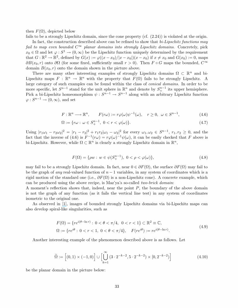
then F (Ω), depicted belowfails to be a strongly Lipschitz domain, since the cone property (cf. (2.24)) is violated at the origin.

In fact, the construction described above can be refined to show that bi-Lipschitz functions mayfail to map even bounded C∞ planar domains into strongly Lipschitz domains. Concretely, pickx0 ∈ Ω and let ϕ : S1 → (0,∞) be the Lipschitz function uniquely determined by the requirementthat G : R2 → R2, defined by G(x) := ϕ((x− x0)/|x− x0|)(x− x0) if x 6= x0 and G(x0) := 0, maps∂B(x0, r) onto ∂Ω (for some fixed, sufficiently small r > 0). Then F G maps the bounded, C∞

domain B(x0, r) onto the domain shown in the picture above.There are many other interesting examples of strongly Lipschitz domains Ω ⊂ Rn and bi-

Lipschitz maps F : Rn → Rn with the property that F (Ω) fails to be strongly Lipschitz. Alarge category of such examples can be found within the class of conical domains. In order to bemore specific, let Sn−1 stand for the unit sphere in Rn and denote by Sn−1

+ its upper hemisphere.Pick a bi-Lipschitz homeomorphism ψ : Sn−1 → Sn−1 along with an arbitrary Lipschitz functionϕ : Sn−1 → (0,∞), and set

F : Rn −→ Rn, F (rω) := rϕ(ω)ψ−1(ω), r ≥ 0, ω ∈ Sn−1, (4.6)

Ω := rω : ω ∈ Sn−1+ , 0 < r < ϕ(ω). (4.7)

Using |r1ω1 − r2ω2|2 = |r1 − r2|2 + r1r2|ω1 − ω2|2 for every ω1, ω2 ∈ Sn−1, r1, r2 ≥ 0, and thefact that the inverse of (4.6) is F−1(rω) = rϕ(ω)−1ψ(ω), it can be easily checked that F above isbi-Lipschitz. However, while Ω ⊂ Rn is clearly a strongly Lipschitz domain in Rn,

F (Ω) = ρw : w ∈ ψ(Sn−1+ ), 0 < ρ < ϕ(ω), (4.8)

may fail to be a strongly Lipschitz domain. In fact, near 0 ∈ ∂F (Ω), the surface ∂F (Ω) may fail tobe the graph of any real-valued function of n− 1 variables, in any system of coordinates which is arigid motion of the standard one (i.e., ∂F (Ω) is a non-Lipschitz cone). A concrete example, whichcan be produced using the above recipe, is Maz’ya’s so-called two-brick domain:A moment’s reflection shows that, indeed, near the point P , the boundary of the above domainis not the graph of any function (as it fails the vertical line test) in any system of coordinatesisometric to the original one.

As observed in [1], images of bounded strongly Lipschitz domains via bi-Lipschitz maps canalso develop spiral-like singularities, such as

F (Ω) = rei(θ−ln r) : 0 < θ < π/4, 0 < r < 1 ⊂ R2 ≡ C,

Ω := reiθ : 0 < r < 1, 0 < θ < π/4, F (reiθ) := rei(θ−ln r).(4.9)

Another interesting example of the phenomenon described above is as follows. Let

Ω :=[(0, 1) × (−1, 0)

]∪[ ∞⋃

k=1

(3 · 2−k−2, 5 · 2−k−2) × [0, 2−k−2)]

(4.10)

be the planar domain in the picture below:

33

It is not difficult to see that the uniformity of the cone condition is violated in any neighborhoodof the origin, so Ω is not a strongly Lipschitz domain. Nonetheless, on p. 19 of [16], Maz’ya hasconstructed a bi-Lipschitz map F : R2 → R2 with the property that Ω = F ((0, 1) × (0, 1)).

The examples presented thus far raise the following interesting issue: give an intrinsic descrip-tion of the class of images of bounded strongly Lipschitz domains under bi-Lipschitz mappings. Fromthe discussion in the next subsection (and §5.1) it follows that this is a subclass of the collectionof all bounded NTA domains with Ahlfors regular boundaries, and which have Lipschitz reflectionsin a collar neighborhood of their boundaries. As a related matter, it is natural to conjecture thatany bounded strongly Lipschitz domain is the bi-Lipschitz image of a bounded C∞ domain. Thisis certainly true for bounded, starlike strongly Lipschitz domains.

Turning to positive results, we shall now prove that bi-Lipschitz homeomorphisms which arealso C1-diffeomorphisms of the space do preserve the class of bounded Lipschitz domains. As theabove discussion shows, this result is in the nature of best possible.

Theorem 4.1. Assume that Ω ⊂ Rn is an open set, O ⊆ Rn is an open neighborhood of Ω, andF : O → Rn is a C1-diffeomorphism onto its image.

Then, if Ω is strongly Lipschitz near x0 ∈ ∂Ω, it follows that F (Ω) is strongly Lipschitz nearF (x0) ∈ ∂F (Ω) as well. Consequently, if Ω is locally strongly Lipschitz, then so is Ω := F (Ω).

In particular, if Ω ⊂ Rn is a bounded strongly Lipschitz domain, O ⊆ Rn is an open neighborhoodof Ω, and F : O → Rn is a C1-diffeomorphism then Ω := F (Ω) is a strongly Lipschitz domain.Furthermore, the Lipschitz character of Ω is controlled in terms of the Lipschitz character of Ω,Lip (F,Ω) and Lip (F−1, F (Ω)).

Proof. Working with Ω replaced by Ω ∩ C, where C is a suitable coordinate cylinder near x0, thereis no loss of generality in assuming that Ω itself is a bounded strongly Lipschitz domain. Note

that Ω := F (Ω) ⊆ Rn is a bounded, open set which, thanks to (2.26), satisfies ∂Ω = ∂(Ω). ByTheorem 3.2, this set is also of locally finite perimeter, and we denote by ν, σ the outward unitnormal and surface measure on ∂Ω.

Consequently, by Theorem 2.4 and Lemma 5.5, it suffices to show that, given x ∈ ∂Ω, there isa continuous vector field transversal to ∂Ω near F (x). However, if X is a continuous vector fieldwhich is transversal to ∂Ω near x, then X := [(DF )F−1](X F−1) will do the job (assuming thatF is orientation preserving). Indeed, if ν is the outward unit normal on ∂Ω then (3.23), (2.12),(3.3) and (3.24) imply that, for a sufficiently small compact neighborhood Ux of x,

X · ν = [(DF ) F−1](X F−1) · (DF−1)>(ν F−1)

‖(DF−1)>(ν F−1)‖

=(X F−1) · (ν F−1)

‖(DF−1)>(ν F−1)‖ ≥ κ

‖(DF ) F−1‖ ≥ κ

Lip (F,Ux)> 0, (4.11)

F∗σ-a.e. (hence, σ-a.e., by (3.17)) near F (x).

We conclude this subsection by presenting the following result, which should be compared withthe criterion (i)-(ii), characterizing the class of bounded C 1 domains, discussed near the beginningof §4.1.

Corollary 4.2. For a nonempty, proper open subset Ω of Rn, the following are equivalent:

(a) Ω is a locally strongly Lipschitz domain;

34

(b) For every point x0 ∈ ∂Ω there exist an open neighborhood U of x0, a C1-diffeomorphismF : Rn → Rn, and numbers b, c > 0, satisfying the following properties:

(i) F (x0) = 0, and F (U) is the open cylinder Cb,c := (x′, t) : |x′| < b, |t| < c;(ii) there exists a Lipschitz function ϕ : Rn−1 → R with ϕ(0) = 0 and |ϕ(x′)| < c if |x′| ≤ b,

and for which

F (U ∩ Ω) = Cb,c ∩ (x′, t) : x′ ∈ Rn−1, t > ϕ(x′). (4.12)

(c) For every point x0 ∈ ∂Ω there exist an open neighborhood U of x0 along with a C1-diffeomorphismF : U → F (U) such that F (U ∩ Ω) is strongly Lipschitz near F (x0).

Proof. If Ω is a locally strongly Lipschitz domain then, by virtue of Definition 2.2, conditions(i) − (ii) in (b) can be satisfied by choosing F to be a suitable isometry of Rn. This proves that(a) ⇒ (b). Trivially, (b) ⇒ (c). As for the remaining implication, assume that (c) holds. Since theC1-diffeomorphism F−1 maps F (U ∩ Ω) into U ∩ Ω, it follows from Theorem 4.1 that the latterdomain is strongly Lipschitz near x0. Being a locally strongly Lipschitz domain is, however, alocal property of the boundary, so may further conclude that Ω itself is a locally strongly Lipschitzdomain.

Let M be a topological manifold of (real) dimension n, equipped with a C 1 atlas A. Call anopen set Ω ⊆ M a locally strongly Lipschitz domain relative to A if for every x0 ∈ ∂Ω there existsa local chart (U, h) ∈ A with x0 ∈ U and such that h(U ∩ Ω) ⊆ Rn is a locally strongly Lipschitzdomain near h(x0). Recall that two C1 atlases A1 and A2 are called equivalent if A1 ∪ A2 is alsoa C1 atlas.

Theorem 4.3. Assume that M is a topological manifold of (real) dimension n, and that A is aC1 atlas on M. Also, let Ω be an open subset of M which is a locally strongly Lipschitz domainrelative to A. Then Ω is a locally strongly Lipschitz domain relative to any other C 1 atlas on Mwhich is equivalent to A.

Proof. Let A′ be a C1 atlas on M which is equivalent to A. Then desired conclusion followsfrom Theorem 4.1 applied to the transitions maps between the charts of A′ and A (which are C1

diffeomorphisms).

4.2 Regular SKT domains are invariant under C1 diffeomorphisms

We remind the reader that a closed set Σ ⊂ Rn is said to be Ahlfors regular provided there exist0 < a ≤ b <∞ (called Ahlfors constants of Σ) such that

a rn ≤ Hn−1(B(x, r) ∩ Σ

)≤ b rn, (4.13)

for each x ∈ Σ and r ∈ (0,∞). If Σ is compact, we require (4.13) only for r ∈ (0, 1]. Nonetheless,(4.13) continues to hold in this case (albeit with possibly different constants) for each 0 < r <diamΣ. An open set Ω ⊂ Rn is said to be an Ahlfors regular domain provided ∂Ω is Ahlforsregular. Note that, by (2.10), an Ahlfors regular domain Ω ⊂ Rn satisfying

35

Hn−1(∂Ω \ ∂∗Ω) = 0 (4.14)

is of locally finite perimeter and σ = Hn−1b∂Ω.Recall that every locally strongly Lipschitz domain is locally starlike. For our purposes here,

we shall need a curvilinear, scale invariant version of this property. Following [10], we make thefollowing.

Definition 4.1. Let Ω ⊂ Rn be an open set. This is said to satisfy a local John condition ifthere exist θ ∈ (0, 1) and R > 0 (required to be ∞ if ∂Ω is unbounded), called the John constants ofΩ, with the following significance. For every p ∈ ∂Ω and r ∈ (0, R) one can find pr ∈ B(p, r) ∩ Ω,called John center relative to ∆(p, r) := B(p, r)∩∂Ω, such that B(pr, θr) ⊂ Ω and with the propertythat for each x ∈ ∆(Q, r) one can find a rectifiable path γx : [0, 1] → Ω, whose length is ≤ θ−1r andsuch that

γx(0) = x, γx(1) = pr, and dist (γx(t), ∂Ω) > θ |γx(t) − x| ∀ t ∈ (0, 1]. (4.15)

Finally, Ω is said to satisfy a two-sided local John condition if both Ω and Rn \ Ω satisfy a localJohn condition.

Lemma 4.4. Bi-Lipschitz mappings preserve the class of Ahlfors regular domains, the class ofdomains for which (4.14) holds, as well as the class of bounded domains satisfying a two-sided localJohn condition.

Proof. This is a direct consequence of (3.14) and (3.2).

Our next result deals with the class of regular SKT (Semmes-Kenig-Toro) domains in Rn.Although intuitively suggestive, the actual definition of this class of domains is somewhat technical.Thus, in order to avoid a lengthy digression we defer such a discussion to the appendix, §5 (wewill, however, employ already the terminology introduced there). Our goal here is to show that theclass of bounded regular SKT domains is invariant under C 1-diffeomorphisms.

Theorem 4.5. If Ω ⊂ Rn is a bounded regular SKT domain and F is a C1-diffeomorphism of Rn,then Ω := F (Ω) is also a (bounded) regular SKT domain.

In order to facilitate the subsequent presentation, we introduce the following notation. Givenx ∈ ∂Ω, 0 < R < diam ∂Ω and f ∈ L1

loc(∂Ω, dσ), define

∆(x,R) := B(x,R) ∩ ∂Ω, f∆(x,R) :=

∫−

∆(x,R)f dσ, (4.16)

‖f‖∗,R := supx∈∂Ω

supρ∈(0,R)

(∫−

∆(x,ρ)|f(y) − f∆(x,ρ)|2 dσ(y)

)1/2. (4.17)

When the center x is understood from the context, or irrelevant, we abbreviate ∆R := ∆(x,R).Finally, set

‖f‖BMO(∂Ω,dσ) := sup ‖f‖∗,R : R ∈ (0,diam Ω). (4.18)

The main estimate used in the proof of Theorem 4.5 is contained in the proposition below,which is itself of independent interest.

36

Proposition 4.6. Assume that Ω ⊂ Rn is a domain of locally finite perimeter with the property thatits surface measure, σ, is doubling. Denote by [σ] the doubling constant of σ and by ν the outwardunit normal on ∂Ω. Next, fix an open neighborhood O ⊆ Rn of Ω and assume that F : O → Rn

is a bi-Lipschitz C1-diffeomorphism. Set Ω := F (Ω) and denote by σ, ν the surface measure andoutward unit normal on ∂Ω. Finally, assume that there exists Ro > 0 with the property that

‖ν‖∗,Ro ≤ δ1, for some δ1 sufficiently small relative [σ], (4.19)

‖DF‖∗,Ro ≤ δ2 for some δ2 sufficiently small relative to [σ], LipF , LipF−1. (4.20)

Then there exist C0, C > 0 and δ > 0, depending only on the Lipschitz constants of F , F −1 and[σ] with the property that

‖ν‖∗,R ≤ C0(‖DF‖∗,CR + ‖ν‖∗,CR), ∀R ∈ (0, δ Ro). (4.21)

Proof. To get started, recall from Proposition 3.6 that σ is also doubling, and that in fact (3.84)holds. Also, generally speaking,

∫−

∆R

∣∣∣(DF )−1 −∫−

∆R

(DF )−1 dσ∣∣∣2dσ

≤∫−

∆R

|(DF )−1|∣∣∣In×n − (DF )

(∫−

∆R

(DF )−1 dσ)∣∣∣

2dσ

≤ C

∫−

∆R

∣∣∣(DF − (DF )∆R)(∫−

∆R

(DF )−1 dσ)∣∣∣

2dσ

+C∣∣∣∫−

∆R

(In×n − (DF )∆R(DF )−1) dσ

∣∣∣2

≤ C‖DF‖2∗,R + C

∫−

∆R

|DF − (DF )∆R|2|(DF )−1|2 dσ

≤ C‖DF‖2∗,R, (4.22)

for every R > 0, which shows that whenever (4.20) holds we also have

‖(DF )−1‖∗,Ro ≤ Cδ2, ∀R ∈ (0, Ro), (4.23)

where C depends only on Ω and LipF−1.Next, for each R ∈ (0,diam Ω) and x ∈ ∂Ω, set

ν∗x,R(y) := supρ∈(0,R)

∫−

∆(x,ρ)|ν(z) − ν∆(x,2R)| dσ(z), y ∈ ∂Ω. (4.24)

We then obtain

ν∗x,R(y) ≤M(|ν − ν∆(x,2R)|1∆(x,2R)

)(y), ∀ y ∈ ∆(x,R), (4.25)

37

where M is the Hardy-Littlewood maximal function on ∂Ω. Note that ∂Ω, when equipped withthe Euclidean distance and measure σ, becomes a space of homogeneous type. Thus, from theboundedness of M on L2(∂Ω, dσ), John-Nirenberg’s inequality and (4.25), we may conclude that

(∫−

∆(x,R)|ν∗x,R(y)|2 dσ(y)

)1/2≤ C

(∫−

∆(x,2R)|ν(y) − ν∆(x,2R)|2 dσ(y)

)1/2≤ C‖ν‖∗,2R. (4.26)

Fix now x0 ∈ ∂Ω and R ∈ (0, δ Ro), where δ ∈ (0, 1/2) is a sufficiently small constant, dependingonly on Ω, LipF and LipF−1, which will be specified later. Then (4.19) and (4.26) show that thereexists y0 ∈ ∆(x0, R) such that |ν(y0)| = 1 and ν∗x0,R(y0) ≤ 1/2, assuming δ1 small. Since byLebesgue’s Differentiation Theorem |ν(y0) − ν∆(x0,2R)| ≤ ν∗x0,R(y0), this forces

12 ≤ |ν∆(x0,2R)| ≤ 1, ∀R ∈ (0, δ Ro). (4.27)

Going further, set

A(x) := (DF−1)>(F (x)) = [(DF (x))−1]>, x ∈ Rn. (4.28)

Running a similar argument to the one used in the paragraph above for the matrix-valued functionA, with the help of (4.22) we also obtain |A(y0) −A∆(x0,2R)| ≤ Cδ2, where C depends only on thebi-Lipschitz constants of F and [σ]. Thus, assuming that δ2 is small, relative to these quantities,we see that

A∆(x0,R) is an invertible n× n matrix, for every R ∈ (0, δ Ro). (4.29)

For R ∈ (0, δ Ro), x0 ∈ ∂Ω and a vector ~c ∈ Rn with ‖~c‖ = 1, to be specified momentarily, wemay use (3.84) and (3.24) in order to estimate

∫−

B(F (x0),R)∩∂ eΩ|ν − ~c|2 dσ

≤ C

∫−

∆(x0,CR)

∣∣∣(DF−1)>(F (x))ν(x) − ‖(DF−1)>(F (x))ν(x)‖~c∣∣∣2|det (DF )(x)| dσ(x)

≤ C

∫−

∆(x0,CR)

∣∣∣A(x)ν(x) − ‖A(x)ν(x)‖~c∣∣∣2dσ(x)

≤ C

∫−

∆(x0,CR)

∣∣∣A∆(x0,CR)ν(x) − ‖A∆(x0,CR)ν(x)‖~c∣∣∣2dσ(x) + C‖A‖∗,CR

≤ C

∫−

∆(x0,CR)

∣∣∣A∆(x0,CR)ν∆(x0,CR) − ‖A∆(x0,CR)ν∆(x0,CR)‖~c∣∣∣2dσ + C‖A‖∗,CR + C‖ν‖∗,CR

= C(‖A‖∗,CR + ‖ν‖∗,CR), (4.30)

for some C which depends exclusively on the Lipschitz constants of F and F −1, if we take

38

~c :=A∆(x0,CR)ν∆(x0,CR)

‖A∆(x0,CR)ν∆(x0,CR)‖. (4.31)

Note that by (4.27) and (4.29), ~c is well-defined, granted that δ is sufficiently small.To summarize, (4.30), (4.28) and (4.22) give

‖ν‖∗,R ≤ C0(‖DF‖∗,CR + ‖ν‖∗,CR) (4.32)

if R ∈ (0, δ Ro) with δ > 0 small, for some constants C0, C > 0 depending only on the Lipschitzconstants of F and F−1.

Let us digress for a moment and point out that, as above proof shows, ‖ν‖BMO(∂ eΩ,deσ)

is small

if ‖DF‖BMO (∂Ω,dσ) and ‖ν‖BMO (∂Ω,dσ) are sufficiently small (relative to the Lipschitz constants ofF , F−1, and the doubling constant of σ). Note that ‖ν‖BMO (∂Ω,dσ) ≤ 1 can only happen when ∂Ωis not compact (since, otherwise,

∫∂Ω ν dσ = 0 forces the opposite inequality).

With Proposition 4.6 in hand, it is easy to finish the

Proof of Theorem 4.5. Lemma 4.4 ensures that Ω is a bounded Ahlfors regular domain, whichsatisfies a local two-sided John condition and for which (4.14) holds. Keeping in mind the charac-terization from Theorem 5.2, it remains to show that ν ∈ VMO (∂Ω, dσ), i.e., that

lim supR→0+

(sup

x0∈∂ eΩ

inf~c∈Rn

(∫−

B(F (x0),R)∩∂ eΩ|ν − ~c|2 dσ

)1/2)

= 0. (4.33)

This, however, is a consequence of (4.21), the membership of ν in VMO(∂Ω, dσ), and the fact that,since DF is continuous, its oscillations converge to zero as the radii of the balls go to zero.

Remark 1. The invariance result for the class of bounded regular SKT domains presented inTheorem 4.5 is sharp, as this class is not, generally speaking, preserved under bi-Lipschitz mappings.To see this, consider a Lipschitz map ϕ : Sn−1 −→ (0, 1) and define

F : Rn −→ Rn, F (rω) := rϕ(ω)ω, r > 0, ω ∈ Sn−1. (4.34)

As with (4.6), F is readily seen to be bi-Lipschitz, but the domain F (B(0, 1)) is, generally speaking,no more regular than a generic strongly Lipschitz domain (starlike with respect to the origin). Inparticular, the image of the regular SKT domain B(0, 1) under such a mapping F may fail to beitself regular SKT.

Remark 2. Given m ∈ N, define VMO1(Rm) as the space of locally integrable functions in Rm

with the property that (the components of) their distributional gradients belong to Sarason’sspace VMO(Rm). Next, define the class of bounded VMO1 domains following the same recipe asin Definition 2.2 except that, instead of asking that ϕ is Lipschitz, this time we stipulate thatϕ ∈ VMO1(R

n−1). Clearly, bounded C1 domains are bounded VMO1 domains which, in turn,are bounded regular SKT domains (cf. [13], [10] for the latter claim). However, while both theclass of bounded C1 domains, and the class of bounded regular SKT domains are invariant under

39

C1-diffeomorphisms of the Euclidean space, it is easy to produce examples showing that, generallyspeaking, this is not the case for the class of bounded VMO1 domains.

Remark 3. By relying on results established in [10], the argument in the proof of Theorem 4.5 canbe altered to show that the image of a bounded δ-SKT domain Ω ⊂ Rn under a C1-diffeomorphismof the space is δo-SKT for some δo := Cδ with C = C(Ω, F ) > 0, granted that the original δ is, tobegin with, small relative to the John and Ahlfors constants of Ω. Furthermore, a suitable versionfor domains which are not necessarily bounded is valid as well.

A local version of Theorem 4.5 holds as well. More specifically, with terminology introduced inDefinition 5.7, the same type of argument as above allows us to conclude the following.

Theorem 4.7. Let Ω ⊂ Rn be an open set, O ⊆ Rn an open neighborhood of Ω, and F : O → Rn

a C1-diffeomorphism onto its image. If Ω is a regular SKT domain near x0 ∈ ∂Ω, it follows thatF (Ω) is a regular SKT domain near F (x0).

In particular, much as we have done in the case of Lipschitz domains, this allows to define regularSKT domains on manifolds and show that the definition depends only on the intrinsic C 1 structureof the manifold.

4.3 Approximating domains of locally finite perimeter

Let Ω ⊂ Rn be an open set of locally finite perimeter, and fix an open neighborhood O ⊆ Rn ofΩ. As before, we let ν, σ denote, respectively, the outward unit normal and surface measure on∂Ω. Going further, assume that Fj : O → Rn, j ∈ N, is a family of global bi-Lipschitz, orientationpreserving, C1-diffeomorphisms, satisfying

supj∈N

Lip (Fj ,O) <∞, supj∈N

Lip (F−1j , Fj(O)) <∞. (4.35)

Set

Ωj := Fj(Ω), j ∈ N. (4.36)

Then, Proposition 3.1 ensures that each Ωj is a set of locally finite perimeter, and we denote by νj ,σj, respectively, the outward unit normal and surface measure on ∂Ωj, j ∈ N.

Proposition 4.8. Retain the above hypotheses and, in addition, assume that

DFj(x) −→ In×n as j → ∞, for σ-a.e. x ∈ ∂Ω, (4.37)

Fj(x) −→ x as j → ∞, for σ-a.e. x ∈ ∂Ω. (4.38)

Then

νj(Fj(x)) −→ ν(x) as j → ∞, for σ-a.e. x ∈ ∂Ω, (4.39)

and

40

(F−1j )∗σj −→ σ as j → ∞, weakly in M. (4.40)

Furthermore, there exist constants 0 < c1 < c2 <∞, depending only on the quantities in (4.35),along with functions ωj ∈ L∞(∂Ω, dσ), j ∈ N, for which

c1 ≤ ωj ≤ c2 σ-a.e. on ∂Ω, ∀ j ∈ N, (4.41)

ωj −→ 1 as j → ∞, σ-a.e. on ∂Ω, (4.42)

and which satisfy the following additional property for every j ∈ N:

σj(Fj(E)) =

∫

Eωj dσ ∀E ⊂ ∂Ω, Borel set. (4.43)

Proof. From (3.23), for each j ∈ N and σ-a.e. x ∈ ∂Ω, we have

νj(Fj(x)) =(DF−1

j )>(Fj(x))ν(x)

‖(DF−1j )>(Fj(x))ν(x)‖

=[(DFj)

>(x)]−1ν(x)

‖[(DFj)>(x)]−1ν(x)‖ . (4.44)

It is then elementary to deduce (4.39) from (4.37)-(4.38) and (4.35).Next, formula (3.24) gives that for every f ∈ C0(Rn) with compact support contained in O,

and every j ∈ N,

∫f d(F−1

j )∗σj =

∫f F−1

j dσj

=

∫(f F−1

j )‖(DF−1j )>(ν F−1

j )‖ |det (DFj) F−1j | d(Fj)∗σ

=

∫f‖(DF−1

j )> Fj ν‖ |det (DFj)| dσ. (4.45)

Hence, the desired conclusion follows with the help of (4.37)-(4.38), (4.35) and Lebesgue’s Domi-nated Convergence Theorem.

In fact, (4.45) also shows that for every Borel set E ⊂ ∂Ω and j ∈ N,

σj(Fj(E)) =

∫

E‖(DF−1

j )> Fj ν‖ |det (DFj)| dσ (4.46)

so that (4.43) is valid if we set

ωj := ‖[(DF−1j )> Fj ] ν‖ |det (DFj)| on ∂Ω. (4.47)

For this choice it is then easy to verify that (4.41)-(4.42) hold, again, by relying on (4.37)-(4.38)and (4.35).

41

Remark 1. Of course, formula (4.43) further entails that composition with F −1j is an isomorphism

from L1(∂Ωj , dσj) onto L1(∂Ω, dσ) and

∫

∂Ωj

f F−1j dσj =

∫

∂Ωf ωj dσ, ∀ f ∈ L1(∂Ω, dσ). (4.48)

Remark 2. Let Ω ⊂ Rn be arbitrary, and assume that O ⊆ Rn is an open neighborhood of Ω. IfFj : O → Rn, j ∈ N, are bi-Lipschitz maps satisfying (4.35) and for which |Fj(x) − x| → 0 asj → ∞, uniformly for x ∈ Ω, it is then straightforward to check that

∂Ωj −→ ∂Ω and Ωj −→ Ω as j → ∞, (4.49)

in the Hausdorff distance sense (cf. (4.53) below for the definition of the Hausdorff distance betweentwo subsets of Rn). If, on the other hand, DFj(x) → In×n as j → ∞, uniformly for x ∈ ∂Ω, itfollows from (4.44) that

‖νj(Fj(·)) − ν‖L∞(∂Ω,dσ) −→ 0 as j → ∞. (4.50)

In the appendix of [15], Kenig and Toro developed an approximation scheme of a δ-Reifenbergflat domain Ω by Ωj := φj(Ω), j ∈ N, where the φj ’s are certain smooth diffeomorphisms of thespace, of bounded bi-Lipschitz character. In the process, results such as (4.39)-(4.43) are establishedvia somewhat ad hoc methods. An inspection of their proof reveals, however, that the φj ’s satisfysimilar conditions to (4.37)-(4.38), so Proposition 4.8 could be used to substantially simplify theirarguments. In the class of strongly Lipschitz domains, approximation schemes similar to the onediscussed in Proposition 4.8 have been developed in [2], [3], [24]. Below we consider in more detailedthe case when Ω is a bounded strongly Lipschitz domain, and give a concrete recipe for constructinga sequence of C1-diffeomorphisms satisfying (4.37)-(4.38).

To set the stage, assume that Ω ⊂ Rn is a bounded strongly Lipschitz domain, and fix a vectorfield

h ∈ C1(Rn, Sn−1), h globally transversal to ∂Ω. (4.51)

Next, for each t > 0, define the mapping

Ft(x) := x− t h(x), Ft : Rn −→ Rn. (4.52)

Finally, we remind the reader that the Hausdorff distance between two sets A,B ⊂ Rn is definedas

D[A,B] := maxsupdist (a,B) : a ∈ A , supdist (b, A) : b ∈ B

. (4.53)

42

Proposition 4.9. In the context given above, there exist to > 0 along with an open neighborhoodO of Ω, both depending only on Ω and h, with the property that if 0 < t < to then Ft(Ω) is open,Ft : O → Ft(Ω) is a C1-diffeomorphism. In addition,

Ft(Ω) ⊂ Ω, ∀ t ∈ (0, to), (4.54)

and

D[∂Ω , ∂Ft(Ω)] ≤ t, ∀ t ∈ (0, to). (4.55)

In order to facilitate the proof of this result, we isolate in the following lemma an importantstep in this direction

Lemma 4.10. Retain the same context as before and, for each t > 0, define

Ot := x− s h(x) : x ∈ ∂Ω, −t < s < t. (4.56)

Then there exists to > 0, depending only on Ω and h, with the property that

0 < t < to =⇒ Ot is an open set, and ∂Ot = ∂Ot = x± t h(x) : x ∈ ∂Ω. (4.57)

Proof. Fix an arbitrary point x0 ∈ ∂Ω. From Definition 2.2 we know that there exist an isometricsystem of coordinates (x′, s) of Rn, with x0 as the origin, such that ∂Ω coincides near 0 withthe graph of a Lipschitz function ϕ : Rn−1 → R with ϕ(0) = 0. Let us denote by h1, ..., hn thecomponents of h in this new system of coordinates. Thanks to (2.23), the transversality conditionsatisfied by h ensures that

−hn(x′ϕ(x′)) ≥ κ > 0, uniformly for x′ near 0 ∈ Rn−1. (4.58)

In this new system of coordinates, let us also define

G : Rn −→ Rn, G(x′, s) := (x′, ϕ(x′)) − s h(x′, ϕ(x′)). (4.59)

The claim that we make at this stage is that

G is bi-Lipschitz near 0 ∈ Rn. (4.60)

To prove this claim, let us first observe that, schematically,

DG(x′, s) =

∣∣∣∣∣∣∣∣∣∣∣∣∣∣

... −h1

I(n−1)×(n−1)

... −h2

. . . . . ....

...

∇′ϕ(x′)... −hn

∣∣∣∣∣∣∣∣∣∣∣∣∣∣

+ O(s), (4.61)

43

where the components h1, ..., hn of h are evaluated at (x′, ϕ(x′)), and the constant implicit in the“big O” symbol depends only on h and ‖∇′ϕ‖L∞ . As a consequence,

det (DG)(x′, s) = −hn(x′, ϕ(x′)) +O(s). (4.62)

Hence, had ϕ been of class C1, the mapping (4.59) would be invertible near 0 ∈ Rn, by the InverseFunction Theorem. This would clearly entail (4.60).

In the more general situation when ϕ is merely Lipschitz, mollify ϕ to produce a sequence ofC∞ functions ϕj , j ∈ N, such that

ϕj → ϕ in L∞, ∇′ϕj → ∇′ϕ pointwise a.e., and supj∈N

‖∇′ϕj‖L∞ ≤ ‖∇′ϕ‖L∞ . (4.63)

If for each j ∈ N we now consider Gj defined analogously to (4.59) but with ϕ replaced by ϕj ,then there exists a neighborhood U of 0 ∈ Rn with the property that Gj → G uniformly in U .Furthermore, as the previous discussion shows, U can be chosen such that

Gj is bi-Lipschitz in U , with constants independent of j. (4.64)

Now (4.60) follows easily from this and a limiting argument. In turn, (4.60) further implies that

G maps sufficiently small neighborhoods of 0 ∈ Rn into neighborhoods of x0. (4.65)

Next, for each t > 0, let us now consider the mapping

H : ∂Ω × (−t, t) −→ Rn, H(x, s) := x− s h(x). (4.66)

We claim that there exists to > 0 such that

t ∈ (0, to) =⇒ H is a bi-Lipschitz mapping. (4.67)

To justify this, observe first that if an arbitrary point x0 ∈ ∂Ω has been fixed, along with a newsystem of coordinates (x′, s), isometric with the standard one, as at the beginning of the currentproof, then in this new system of coordinates

H(x, s) = G(x′, s), if x = (x′, xn) ∈ ∂Ω is near x0. (4.68)

From this and (4.60) we then deduce that

|H(x, s1) −H(y, s2)| ≥ C(|x′ − y′| + |s1 − s2|), whenever

x = (x′, xn), y = (y′, yn) ∈ ∂Ω are near x0, and s1, s2 are near 0.(4.69)

Since, in the above context, |xn − yn| = |ϕ(x′) − ϕ(y′)| ≤ C|x′ − y′|, (4.69) further improves to

44

|H(x, s1) −H(y, s2)| ≥ C|(x, s1) − (y, s2)|,if x, y ∈ ∂Ω are near x0, and s1, s2 are near 0.

(4.70)

Since the reverse inequality in (4.70) is a simple consequence of (4.66), this shows that H in (4.66)is locally bi-Lipschitz. It is then easy to show that the claim in (4.67) holds, as soon as we provethat H in (4.66) is one-to-one.

To this end, assume that x1, x2 ∈ ∂Ω, s1, s2 ∈ (−t, t) are such that H(x1, s1) = H(x2, s2). Itfollows that |x1 − x2| = |s1 h(x1)− s2 h(x2)| ≤ |s1|+ |s2| ≤ 2t. Hence, if t ∈ (0, to) for a sufficientlysmall to > 0, this forces x1, x2 to belong to the same coordinate cylinder near a boundary pointx0 (in the terminology of Definition 2.2). Moreover, this coordinate cylinder can be made smallby taking to small. Once this has been established, the local bi-Lipschitzianity of H gives that(x1, s1) = (x2, s2), proving that H is one-to-one. This concludes the proof of (4.67).

Going further, note that

Ot = H(∂Ω × (−t, t)). (4.71)

As a consequence of this, (4.65) and (4.68), we may conclude that Ot is open if t ∈ (0, to), if to > 0is sufficiently small. Furthermore, regarding ∂Ω × (−t, t) as an open set in the topological space∂Ω × (−t1, t1), with 0 < t < t1 < to, to > 0 small, then (4.67) gives

∂Ot = ∂[H(∂Ω × (−t, t))] = H(∂(∂Ω × (−t, t)))= H(∂(∂Ω × [−t, t])) = H(∂Ω × ±t) = x± t h(x) : x ∈ ∂Ω. (4.72)

A similar argument shows that ∂Ot = x± t h(x) : x ∈ ∂Ω, finishing the proof of (4.57).

Remark. The proof of Lemma 4.10 is actually more resourceful than its actual statement indicates.For example, it gives that for to > 0 small and t ∈ (0, to),

O±t := x∓ s h(x) : x ∈ ∂Ω, 0 < s < t (4.73)

are open sets with ∂O±t := x∓ t h(x) : x ∈ ∂Ω. Also, the application

R : Ot −→ Ot, R(x− s h(x)) := x+ s h(x), x ∈ ∂Ω, s ∈ (−t, t), (4.74)

is well-defined, Lipschitz, involutive, fixes ∂Ω, and maps O±t onto O∓

t (that is, R is a Lipschitzreflection across the boundary, ∂Ω, in a collar neighborhood of it).

We are now prepared to present the

Proof of Proposition 4.9. To begin with, we note that there exists to > 0 such that Ft is aC1-diffeomorphism mapping an open neighborhood O of Ω onto an open subset of Rn. Indeed,Ft is of class C1 in RRn for each t and, given a bounded, open neighborhood O of Ω, we have|DFt(x) − In×n| ≤ t ‖Dh‖L∞(O), for any x ∈ O. Thus, DFt is invertible at every point in O ift ∈ (0, to) with to > 0 sufficiently small. As a consequence, the Inverse Function Theorem can

45

be invoked to conclude that Ft is locally a C1-diffeomorphism, if t ∈ (0, to). In particular, Ft(O)is an open subset of Rn for each t ∈ (0, to). To conclude that actually Ft : O → Ft(O) is a C1-diffeomorphism, it suffices to show that this map is one-to-one. Given we know this at the locallevel, this can be easily arranged (using the explicit formula in (4.52)) by ensuring that to is smallenough.

Next, from (4.52) and the fact that F is a C1-diffeomorphism (hence, in particular, a topologicalhomeomorphism), we obtain

∂Ft(Ω) = Ft(∂Ω) = x− t h(x) : x ∈ ∂Ω, t ∈ (0, to). (4.75)

From this and (4.53), the estimate (4.55) readily followsNext, retaining notation used in Lemma 4.10, let us write

∂(Ω \ Ot) = Ω ∩ ∂Ot = x− t h(x) : x ∈ ∂Ω = ∂Ft(Ω). (4.76)

Above, the first equality is a consequence of Lemma 5.7 (specifically, (5.22) applied with A := Ωand B := Ot). The second equality then follows from (4.57) and (2.57), while the third is containedin (4.75).

As far as (4.54) is concerned, working in each connected component of Ω, there is no loss ofgenerality in assuming that Ω itself is connected. Assuming that this is the case, we now bring inLemma 5.8, considered for the open sets O1 := Ft(Ω) and O2 := Ω\Ot. Note that O1 is connected,since Ω is connected and Ft is continuous. The conclusion then is that: either (i) Ft(Ω) and Ω \Ot

are disjoint, or (ii) Ft(Ω) ⊆ Ω \ Ot. To rule out the first eventuality, it suffices to observe that ifx ∈ Ω is such that r := dist (x, ∂Ω) > 2to, then for each t ∈ (0, to) we have Ft(x) ∈ B(x, r/2) ⊂ Ω,and dist (Ft(x), ∂Ω) > to. The latter condition ensures that Ft(x) does not belong to

Ot = Ot ∪ ∂Ot = x− s h(x) : x ∈ ∂Ω, −t ≤ s ≤ t, (4.77)

since any point is the last set above is at distance ≤ to from ∂Ω, granted that 0 < t < to. Thusaltogether, Ft(x) ∈ Ω\Ot, proving that (i) above cannot happen if 0 < t < to, with to small enough.Consequently,

Ft(Ω) ⊆ Ω \ Ot, ∀ t ∈ (0, to), (4.78)

if to small. Thus, Ft(Ω) ⊆ Ω \ Ot if t ∈ (0, to), and (4.54) follows from this and Lemma 5.9 usedwith O := Ot. This concludes the proof of Proposition 4.9.

Remark. By further refining some of the arguments above, it is possible to show that, in fact,

Ft(Ω) = Ω \ Ot, ∀ t ∈ (0, to), (4.79)

if to small. To see this, we invoke (4.66)-(4.67), (4.71) and the fact that ∂Ω is locally (up to anisometry) a Lipschitz graph, in order to conclude that for each x ∈ ∂(Ω\O t) there exists r > 0 withthe property that B(x, r) \ ∂(Ω \Ot) consists of two open connected components, one contained inΩ∩Ot and the other in Ω \Ot. Given that, as we have already shown, Ft(Ω) is a Lipschitz domain

46

for which ∂Ft(Ω) = ∂(Ω \ Ot) (cf. (4.76)), we may conclude that the sets Ft(Ω) and Ω \ Ot agreein the neighborhood of any point on their common boundary. Then (4.79) follows from this andLemma 5.10.

We are now in a position to state an approximation result in the spirit of Calderon’s work in[2].

Proposition 4.11. Consider a bounded strongly Lipschitz domain Ω in Rn with surface measureσ and outward unit normal ν, and let h be a C1 vector field in Rn satisfying

|h(x)| = 1 and 〈h(x), ν(x)〉 ≥ κ for σ-a.e. x ∈ ∂Ω, (4.80)

where κ ∈ (0, 1) is a fixed constant. Also, for each t > 0, let Ωt be the subset of Ω defined by

Ωt := x− t h(x) : x ∈ Ω. (4.81)

Then there exists to > 0, depending only on the Lipschitz character of Ω, the Lipschitz constantof h in a compact neighborhood of Ω, n and κ, such that the following properties hold.

(i) Whenever 0 < t < to, Ωt is a bounded strongly Lipschitz domain with

Ωt ⊆ Ω and ∂Ωt = x− t h(x) : x ∈ ∂Ω. (4.82)

(ii) There exists a covering of ∂Ω with finitely many coordinate cylinders which also form a familyof coordinate cylinders for ∂Ωt, for each t ∈ (0, to). Moreover, for each such cylinder C, if ϕand ϕt are the corresponding Lipschitz functions whose graphs describe the boundaries of Ωand Ωt, respectively, in C, then ‖∇ϕt‖L∞ ≤ C‖∇ϕ‖L∞ and ∇ϕt → ∇ϕ pointwise σ-a.e. ast→ 0+;

(iii) Consider the mapping defined by

Λt : ∂Ω −→ ∂Ωt, Λt(x) := x− t h(x), x ∈ ∂Ω. (4.83)

Then Λt is a bi-Lipschitz map for each t ∈ (0, to) and the Lipschitz constants of Λt and Λt−1

are uniformly bounded in t;

(iv) For every t ∈ (0, to) and every x ∈ ∂Ω, Λt(x) approaches x as t → 0+ along a transversaldirection (hence, nontangentially),

supx∈∂Ω

|x− Λt(x)| ≤ Ct, (4.84)

for some finite, positive constant C = C(Ω, h).

47

(v) For each t ∈ (0, to), there exist positive functions ωt : ∂Ω → R+, bounded away from zero andinfinity uniformly in t, such that, for any measurable set E ⊂ ∂Ω,

∫

Eωt dσ =

∫

Λt(E)dσt, (4.85)

where dσt denotes the surface measure on ∂Ωt. In addition,

supx∈∂Ω

|1 − ωt(x)| ≤ Ct, ∀ t ∈ (0, to), (4.86)

for some finite, positive constant C = C(Ω, h).

(vi) If νt is the outward unit normal vector to ∂Ωt then, with C as above,

supx∈∂Ω

|ν(x) − νt(Λt(x))| ≤ Ct, ∀ t ∈ (0, to). (4.87)

Finally, a similar approximation result from the outside, i.e., with domains Ωt ⊃ Ω, holds aswell.

Proof. This is largely a direct consequence of Theorem 4.1, Proposition 4.8 and Proposition 4.9.The pointwise convergence in (iii) can be seen from (2.73) and (3.23). The fact that Λt(x) → xnontangentially as t→ 0+ is seen from (2.57) and the remark made on that occasion.

We conclude by discussing a refined version of Proposition 4.8, using resulst from the secondpart of §3. Recall definition (3.61).

Proposition 4.12. Retain the same context as in Proposition 4.8 and, instead of (4.37)-(4.38),assume that there is a bi-Lipschitz mapping F : O → Rn for which

d∂∗ΩFj(x) −→ d∂∗ΩF (x) as j → ∞, for σ-a.e. x ∈ ∂Ω, (4.88)

Fj(x) −→ F (x) as j → ∞, for σ-a.e. x ∈ ∂Ω. (4.89)

Let ν, σ denote the outward unit normal and surface measure on the boundary of Ω := F (Ω). Then

νj(Fj(x)) −→ ν(F (x)) as j → ∞, for σ-a.e. x ∈ ∂Ω, (4.90)

and

(F−1j )∗σj −→ (F−1)∗σ as j → ∞, weakly, as Radon measures. (4.91)

When Ω is a bounded Lipschitz domain, then (4.90)-(4.91) hold when (4.88) is replaced by

∇tanFj(x) −→ ∇tanF (x) as j → ∞, for σ-a.e. x ∈ ∂Ω, (4.92)

where ∇tan is the tangential gradient on the C1 surface ∂Ω. In this latter scenario, formulas(3.75)-(3.76) hold.

48

Proof. The first part follows much as Proposition 4.8, with the help of Theorem 3.4 and (3.72).Then the second part is a consequence of (4.90)-(4.91) and (3.75)-(3.76).

Below is a corollary of this result which is quite useful in applications.

Corollary 4.13. Assume that ϕ : Sn−1 → (0,∞) is a Lipschitz function and consider the open setΩ := rω : 0 ≤ r < ϕ(ω), ω ∈ Sn−1 ⊆ Rn. Then Ω is a strongly Lipschitz domain, with outwardunit normal given by

ν(ϕ(ω)ω) =ϕ(ω)ω − (∇tanϕ)(ω)√|(∇tanϕ)(ω)|2 + |ϕ(ω)|2

, for a.e. ω ∈ Sn−1, (4.93)

(where ∇tanϕ denotes the tangential gradient of ϕ on Sn−1), and surface measure σ satisfying

∫

∂Ωf dσ =

∫

Sn−1

f(ωϕ(ω))ϕ(ω)√

|(∇tanϕ)(ω)|2 + |ϕ(ω)|2 dω, (4.94)

for every nonnegative, measurable function f on ∂Ω.

Proof. Define Fϕ : Rn → Rn by setting Fϕ(rω) := rϕ(ω)ω, if r ≥ 0, ω ∈ Sn−1. It can thenbe easily checked that Fϕ is a bi-Lipschitz mapping with the property that (Fϕ)−1 = F1/ϕ. Also,Ω = Fϕ(B(0, 1)). Thus, Ω is a bounded domain of finite perimeter by Proposition 3.1. For t ∈ (0, 1),consider the kernel

kt(x, y) :=1

an

1 − t2

|tx− y|n , x, y ∈ Rn, (4.95)

where an is the area of Sn−1. Since kt(x, y) = K(tx, y), where K(x, y) = 1an

1−|x|2|x−y|n is the (harmonic)

Poisson kernel for the unit ball, it follows that kt(ω, ω′) acts as an approximate identity on Sn−1

as t→ 1−. Set

ϕt(ω) :=

∫

Sn−1

kt(ω, ω′)ϕ(ω′) dω′, ω ∈ Sn−1, (4.96)

so that ϕt ∈ C∞(Sn−1). As (xj

|x|∂xk− xk

|x|∂xj)kt(x, y) = −(

yj

|y|∂yk− yk

|y|∂yj)kt(x, y) for each pair of

indices j, k ∈ 1, ..., n, we also obtian

ϕt(ω) −→ ϕ(ω) and ∇tanϕt(ω) −→ ∇tanϕ(ω) as t→ 1− for a.e. ω ∈ Sn−1. (4.97)

Thus, Fϕt : Rn\0 → Rn\0 is a C∞ diffeomorphism with the property that Fϕt → Fϕ pointwiseon Sn−1. Also, a direct calculation shows that for each j ∈ 1, ..., n,

∇tan(Fϕt)j(ω) = ϕt(ω)(ej − ωjω) + ωj(∇tanϕt)(ω), ω ∈ Sn−1, (4.98)

which, in turn, can be used to conclude that ∇tanFϕt(ω) → ∇tanFϕ(ω) as t→ 1− for a.e. ω ∈ Sn−1.Using the readily checked formula

49

(DFϕt)(ω) = ϕt(ω)In×n + ω ⊗ (∇tanϕt)(ω), ω ∈ Sn−1, (4.99)

one can then employ (3.23) in order to conclude that the outward unit normal to Ωt := Fϕt(B(0, 1))is given by

νt(Fϕt(ω)) =ϕt(ω)ω − (∇tanϕt)(ω)√|(∇tanϕt)(ω)|2 + |ϕt(ω)|2

, for ω ∈ Sn−1. (4.100)

With this in hand, (4.93) follows from (4.90), by letting t→ 1− and invoking (4.97). The argumentfor (4.94) is similar, with (3.24) and (4.91) involved this time.

Finally, to prove that Ω is a strongly Lipschitz domain, it suffices to observe ∂Ω = ∂Ω (itselfa consequence of the fact that Ω is the image of B(0, 1) under the bi-Lipschitz map Fϕ) and thatX(x) := x/|x|, x ∈ Rn \ 0, is a continuous vector field near ∂Ω satisfying

X(ϕ(ω)ω) · ν(ϕ(ω)ω) =ϕ(ω)√

|(∇tanϕ)(ω)|2 + |ϕ(ω)|2

≥ infSn−1 ϕ√‖∇tanϕ‖2∞ + ‖ϕ‖2∞

> 0, (4.101)

for a.e. ω ∈ Sn−1. Then the desired conclusion is provided by Theorem 2.3.

In the lemma on p. 17 of [16] it is established that if Ω ⊂ Rn is an open set which is starlike withrespect to the ball B(0, ρ), for some ρ > 0, then there exists a Lipschitz function ϕ : Sn−1 → (0,∞)such that Ω = rω : 0 ≤ r < ϕ(ω), ω ∈ Sn−1. As a consequence of this and Corollary 4.13 wethen obtain:

Proposition 4.14. If Ω is an open, proper subset of Rn, which is starlike with respect to someball, then Ω is a strongly Lipschitz domain.

5 Appendix

5.1 Reifenberg flat, nontangentially accessible, and Semmes-Kenig-Toro do-

mains

For the convenience of the reader, here we summarize the definitions of Reifenberg flat, NTA andSKT domains. To keep the technicalities to a minimum, we shall only consider here the case ofbounded domains. Our presentation follows closely that of [14], [15], with also some influence from[10]. We momentarily digress for the purpose of explaining the terminology used in this subsection.What we here call SKT domains have been previously called in the literature chord arc domains.The latter notion originated in the two dimensional setting, where the defining condition is thatthe length of a boundary arc between two points does not exceed a fixed multiple of the length ofa chord between these points. In higher dimensions, where this phenomenon becomes somewhatmore sophisticated, this notion originated in S. Semmes [22] and was further developed in [13]–[15].In the higher dimensional setting, this “chord arc” designation no longer adequately captures the

50

essential features of such domains, and in [10] we have proposed to call them SKT (Semmes-Kenig-Toro) domains. Likewise, we have relabeled what was previously called in these papers chord arcdomains with vanishing constant, calling them regular SKT domains.

Recall the definition of the Hausdorff distance from (4.53).

Definition 5.1. Let Σ ⊂ Rn be a compact set and let δ ∈ (0, 14√

2). We say that Σ is δ-Reifenberg

flat if there exists R > 0 such that for every x ∈ Σ and every r ∈ (0, R] there exists a (n − 1)-dimensional plane L(x, r) which contains x and such that

1

rD[Σ ∩B(x, r) , L(x, r) ∩B(x, r)] ≤ δ. (5.1)

Definition 5.2. We say that a bounded open set Ω ⊂ Rn has the separation property if thereexists R > 0 such that for every x ∈ ∂Ω and r ∈ (0, R] there exists an (n − 1)-dimensional planeL(x, r) containing x and a choice of unit normal vector to L(x, r), ~nx,r, satisfying

y + t ~nx,r ∈ B(x, r) : y ∈ L(x, r), t < − r4 ⊂ Ω,

y + t ~nx,r ∈ B(x, r) : y ∈ L(x, r), t > r4 ⊂ Rn \ Ω.

(5.2)

Moreover, if Ω is unbounded, we also require that ∂Ω divides Rn into two distinct connected com-ponents and that Rn \ Ω has a non-empty interior.

Definition 5.3. Let Ω ⊂ Rn be a bounded open set and δ ∈ (0, δn). Call Ω a δ-Reifenberg flat

domain if Ω has the separation property and ∂Ω is δ-Reifenberg flat.

For example, given δ > 0, a strongly Lipschitz domain with a sufficiently small Lipschitzconstant is a δ-Reifenberg flat domain.

Definition 5.4. A bounded open set Ω ⊂ Rn is called an NTA domain provided Ω satisfies a two-sided corkscrew condition (defined in §2), along with a Harnack chain condition.

The Harnack chain condition is defined as follows (with reference to M and R as above). First,given x1, x2 ∈ Ω, a Harnack chain from x1 to x2 in Ω is a sequence of balls B1, . . . , BK ⊂ Ω suchthat x1 ∈ B1, x2 ∈ BK and Bj ∩Bj+1 6= ∅ for 1 ≤ j ≤ K − 1, and such that each Bj has a radiusrj satisfying M−1rj < dist(Bj, ∂Ω) < Mrj. The length of the chain is K. Then the Harnackchain condition on Ω is that if ε > 0 and x1, x2 ∈ Ω ∩ Br/4(z) for some z ∈ ∂Ω, r ∈ (0, R),

and if dist(xj , ∂Ω) > ε and |x1 − x2| < 2kε, then there exists a Harnack chain B1, . . . , BK fromx1 to x2, of length K ≤ Mk, having the further property that the diameter of each ball Bj is≥M−1 min

(dist(x1, ∂Ω),dist(x2, ∂Ω)

).

Finally, call a bounded open set Ω ⊂ Rn a two-sided NTA domain provided both Ω and Rn \Ωare NTA domains.

The following result is proved in §3 of [13].

Proposition 5.1. There exists a dimensional constant δn ∈ (0, 14√

2) with the property that any

bounded domain Ω ⊂ Rn that has the separation property and whose boundary is a δ-Reifenberg flatset, δ ∈ (0, δn), is an NTA-domain.

51

Definition 5.5. Let δ ∈ (0, δn), where δn is as in Theorem 5.1. A bounded set Ω ⊂ Rn of finiteperimeter is said to be a δ-SKT domain if Ω is a δ-Reifenberg flat domain, ∂Ω is Ahlfors regularand there exists r > 0 such that

supx∈∂Ω

(sup

∆⊂∆(x,r)

(∫−

∆|ν − ν∆|2 dσ

)1/2)< δ, (5.3)

with the supremum taken over all surface balls ∆ contained in ∆(x, r) := ∂Ω ∩ B(x, r). Here, asbefore, ν is the measure-theoretic outward unit normal to ∂Ω and ν∆ :=

∫−∆ν dσ.

Definition 5.6. Call a bounded open set Ω ⊂ Rn a regular SKT domain if Ω is a δ-SKT domainfor some δ ∈ (0, δn) and, in addition, ν ∈ VMO(∂Ω, dσ). The last condition means that

lim supr→0+

(supx∈∂Ω

(∫−

∆(x,r)|ν − ν∆(x,r)|2 dσ

)1/2)

= 0. (5.4)

We conclude by recalling a useful, natural characterization of the class bounded regular SKTdomains, recently established in [10]:

Theorem 5.2. Let Ω ⊆ Rn be a bounded open set. Then the following are equivalent:

(i) Ω is a regular SKT domain;

(ii) Ω is a two-sided NTA domain, ∂Ω is Ahlfors regular, and ν ∈ VMO(∂Ω, dσ);

(iii) Ω is a domain with an Ahlfors regular boundary, satisfying a two-sided local John condition(cf. Definition 4.1), and for which ν ∈ VMO(∂Ω, dσ).

Note that any domain with a compact, Ahlfors regular boundary has finite perimeter. Inparticular, it makes sense to talk about its outward unit normal ν and surface measure σ. Infact, there holds σ = Hnb∂Ω. Let us also remark that if the condition ν ∈ VMO (∂Ω, dσ) inTheorem 5.2 is strengthened to ν ∈ C0(∂Ω,Rn), then this result becomes a characterization of C 1

domains (compare with Theorem 2.12).Recall that the conditions demanded in Definition 5.6 are that the domain is δ-Reifenberg flat,

has an Ahlfors regular boundary, and its unit normal is in VMO. Compared with the originaldefinition of a regular SKT domain, the last two characterizations given in Theorem 5.2 has theadvantage of being more economical, in that it avoids stipulating a priori two sources of “regularity”for the boundary, namely that the unit normal has vanishing mean oscillations, and a certain degreeof Reifenberg flatness. Indeed, in the setting of (iii) in Theorem 5.2, Reifenberg flatness has beenreplaced by a two-sided local John condition which is not a flatness/regularity condition. In thecontext of the current paper, this is useful inasmuch it is not clear that the image of a (bounded)δ-Reifenberg flat domain Ω under a C1-diffeomorphism F is a δ′-Reifenberg flat domain, whereδ′ := Cδ, with C depending on F and the geometry of Ω.

We conclude this subsection with a local version of SKT regularity.

Definition 5.7. Let Ω be an open, nonempty, proper subspace of Rn, and assume that x0 ∈ ∂Ω.Call Ω a regular SKT domain near x0 if the following conditions are fulfilled:

52

(i) there exist r0 > 0 and λ > 0 such that B(x0, r0) ∩ Ω is a set of finite perimeter (with surfacemeasure σ and outward unit normal ν), such that Hn−1(∆r) ≈ rn−1 uniformly for any surfaceball ∆r ⊂ B(x0, λr0) ∩ ∂Ω;

(ii) there holds

lim supr→0+

(sup

∆r⊆B(x0,λr0)∩∂Ω

(∫−

∆r

|ν(y) − ν∆r |2 dσ(y))1/2

)= 0; (5.5)

(iii) all points p ∈ B(x0, λr0) ∩ ∂Ω satisfy a condition analogous to the two-sided local John con-dition from Definition 4.1;

This is natural in the sense that a nonempty, bounded open set Ω ⊂ Rn is a regular SKT domainif and only if Ω is a regular SKT domain near each x0 ∈ ∂Ω.

5.2 Cross products and determinants

Let us define the vector product v1 × v2 × · · · × vn−1 of a collection of n − 1 vectors in Rn,v1 = (v11, ..., v1n), . . . , vn−1 = (vn−1 1, ..., vn−1 n), as

v1 × v2 × · · · × vn−1 = det

∣∣∣∣∣∣∣∣∣∣∣

v11 v12 . . . v1n

v21 v22 . . . v2n...

......

...vn−1 1 vn−1 2 . . . vn−1 n

e1 e2 . . . en

∣∣∣∣∣∣∣∣∣∣∣

, (5.6)

where the determinant is understood as being computed by formally expanding it with respect tothe last row, the result being a vector in Rn. As before, e1, ..., en are the vectors of the standardorthonormal basis of Rn. From this, it easily follows that if v1, ..., vn is a positively orientedorthonormal basis in Rn then

v1, ..., vn is a positively oriented orthonormal basis in Rn =⇒ v1 × · · · × vn−1 = vn. (5.7)

Let us also point out that, if vectors v ∈ Rn are identified with 1-forms v# :=∑n

i=1〈v, ei〉 dxi, then

v1 × v2 × · · · × vn−1 = ∗((v1)# ∧ · · · ∧ (vn−1)

#). (5.8)

It is also useful to observe that if v1 = (v11, ..., v1n), . . . , vn = (vn1, ..., vnn) are n vectors in Rn, then

〈v1 × v2 × · · · × vn−1, vn〉 = det

∣∣∣∣∣∣∣∣∣∣∣

v11 v12 . . . v1n

v21 v22 . . . v2n...

......

...vn−1 1 vn−1 2 . . . vn−1 n

vn1 vn2 . . . vnn

∣∣∣∣∣∣∣∣∣∣∣

, (5.9)

i.e., 〈v1×· · ·×vn−1, vn〉 is the (oriented) volume of the parallelopiped spanned by v1, . . . , vn in Rn.

53

Lemma 5.3. For any n× n matrix A, and any collection of n− 1 vectors v1, v2, . . . , vn−1 ∈ Rn,

A>(Av1 × · · · ×Avn−1) = (detA) v1 × · · · × vn−1. (5.10)

Thus, in the particular case when A is an invertible n× n matrix,

Av1 × · · · ×Avn−1 = (detA) (A−1)>(v1 × · · · × vn−1), (5.11)

for every collection of vectors v1, v2, . . . , vn−1 ∈ Rn.

Proof. Fix an arbitrary collection of n− 1 vectors v1, v2, . . . , vn−1 in Rn. Then, making use of theremark just preceding the statement of this lemma, for each vector vn ∈ Rn we may write

〈A>(Av1 × · · · ×Avn−1) , vn〉 = 〈Av1 × · · · ×Avn−1 , Avn〉= oriented volume (span Av1, ..., Avn)= (detA) oriented volume (span v1, ..., vn)= (detA) 〈v1 × · · · × vn−1 , vn〉.

(5.12)

In the third equality above, we have interpreted the volume in question as an integral and haveused a well-known “change of variable” formula (cf., e.g., Lemma 1 on p. 92 in [7]). Since vn ∈ Rn

was arbitrary, the desired conclusions follow from (5.12).

Lemma 5.4. If A is an n× (n− 1) matrix, then

√det (A>A) = |Ae′1 × · · · ×Ae′n−1|, (5.13)

where e′1, . . . , e′n−1 are the vectors of the canonical orthonormal basis in Rn−1.

Proof. Let A = O S be the polar decomposition of A, where S is a (n− 1) × (n− 1) symmetric(i.e., S = S>) matrix, and O is a n × (n − 1) orthogonal (i.e., inner product preserving) matrix.Set V := ORn−1, which is a (n− 1)-plane in Rn, and pick a unit vector v ∈ Rn with the propertythat V ⊕ 〈v〉 = Rn (orthogonal, direct sum).

For each x = (x1, ..., xn) ∈ Rn, write x′ := (x1, ..., xn−1) ∈ Rn−1 and define x′ := (x1, ..., xn−1, 0).We can then extend O, originally viewed as a linear operator O : Rn−1 → Rn, to an operatorO : Rn → Rn (subsequently identified with a n × n matrix) defined by Ox := Ox′ + xnv, ifx = (x1, ..., xn) ∈ Rn. With this convention, O becomes a unitary transformation in Rn. Using theresult in Lemma 5.3, we then compute

|Ae′1 × · · · ×Ae′n−1| = |O(Se′1) × · · · ×O(Se′n−1)| = |O(Se′1) × · · · × O(Se′n−1)|

= |(Se′1) × · · · × (Se′n−1)| = |(detS) en| = |detS|

=√

det (S2) =√

det ((O S)>(O S))

=√

det (A>A), (5.14)

where the fourth equality above is a direct consequence of (5.6).

54

5.3 Some topological lemmas

Lemma 5.5. Let Ω1,Ω2 be two open subsets of Rn, with the property that ∂Ωj = ∂(Ωj), j = 1, 2.Then

∂(Ω1 ∩ Ω2) = ∂(Ω1 ∩ Ω2). (5.15)

Proof. Since ∂(E) = ∂E for any set E ⊂ Rn, the right-to-left inclusion in (5.15) always holds, sothere remains to shows that

∂(Ω1 ∩ Ω2) ⊆ ∂(Ω1 ∩ Ω2). (5.16)

To this end, recall that

∂(A ∩B) ⊆ (A ∩ ∂B) ∪ (∂A ∩B), ∀A,B ⊆ Rn, (5.17)

which further implies

∂(A ∩B) =(∂(A ∩B) ∩A ∩ ∂B

)∪(∂(A ∩B) ∩B ∩ ∂A

). (5.18)

From this, and simple symmetry considerations, we see that (5.16) will follow as soon as we checkthe validity of the inclusion

∂(Ω1 ∩ Ω2) ∩ (Ω1 ∩ ∂Ω2) ⊆ ∂(Ω1 ∩ Ω2). (5.19)

To this end, we reason by contradiction and assume that there exist a point x and a numberr > 0 satisfying

x ∈ ∂(Ω1 ∩ Ω2), x ∈ ∂Ω2, and

either B(x, r) ∩ (Ω1 ∩ Ω2) = ∅, or B(x, r) ⊆ Ω1 ∩ Ω2.(5.20)

Note that if B(x, r) ∩ (Ω1 ∩ Ω2) = ∅ then also B(x, r) ∩ (Ω1 ∩ Ω2) = ∅, contradicting the factthat x ∈ ∂(Ω1 ∩ Ω2). Thus, necessarily, B(x, r) ⊆ Ω1 ∩ Ω2. However, this entails B(x, r) ⊂ Ω2,contradicting the fact that x ∈ ∂Ω2 = ∂(Ω2). This shows that the conditions listed in (5.20) arecontradictory and, hence, proves (5.19).

Lemma 5.6. For every subset Ω of Rn, the implication (2.61) holds.

Proof. From the fact that Ω ⊂ Rn satisfies the exterior corkscrew condition it follows that ∂Ω ⊆[(Ωc)]. This and the readily verified formula (Ωc) = (Ω)c, then yield ∂Ω ⊆ [(Ω)c]. Hence,

∂Ω ⊆ Ω∩ [(Ω)c] = ∂Ω, i.e., ∂Ω ⊆ ∂Ω. Since the opposite inclusion is always true, (2.61) follows.

55

Lemma 5.7. (i) If A,B ⊂ Rn are such that ∂A ⊆ B then

∂(A \ B) ⊆ A ∩ ∂B. (5.21)

(ii) If A,B ⊂ Rn are two sets with the property that ∂A ⊆ B and B ∩ ∂B = ∅ then

∂(A \ B) = A ∩ ∂B. (5.22)

Proof. Note that ∂(A\B) ⊆ A \B ⊆ A. Also, (5.17) gives ∂(A\B) ⊆ (A∩∂(B c))∪(∂A∩Bc). Since∂(Bc) = ∂B and, using the hypotheses, ∂A∩Bc ⊆ B∩Bc = ∂B, we conclude that ∂(A \B) ⊆ ∂B.Thus, (5.21) follows.

As for (5.22), note that A∩∂B = (A∩∂B)∪(∂A∩∂B) = A∩∂B, by hypotheses. Thus, we onlyhave to show that A ∩ ∂B ⊆ ∂(A \ B) = A \B ∩ Ac ∪B. However, A ∩ ∂B ⊆ ∂B ⊆ B ⊆ Ac ∪Band, if B ∩ ∂B = ∅, then also A ∩ ∂B ⊆ A \ B ⊆ A \B. This finishes the proof of the lemma.

Lemma 5.8. Let O1,O2 ⊂ Rn be two open sets such that O1 is connected and ∂O1 = ∂O2. Then

either O1 ∩ O2 = ∅, or O1 ⊆ O2. (5.23)

Proof. Observe that Rn = O2 ∪ (O2)c ∪ ∂O2, mutually disjoint unions, and since O1 ∩ ∂O2 =

O1 ∩ ∂O1 = ∅, we obtain

O1 =(O1 ∩ O2

)∪(O1 ∩ (O2)

c), (5.24)

disjoint union. Thus, since O1 is connected, it follows from (5.24) that O1 ∩O2 is either O1, or theempty set. With this in hand, (5.23) readily follows.

Lemma 5.9. Let Ω,O ⊂ Rn be two open sets with the property that Ω is bounded and ∂Ω ⊆ O.Then

Ω \ O ⊆ Ω. (5.25)

Proof. Since Ω \ O ⊆ Ω = Ω ∪ ∂Ω, disjoint union, it suffices to show that ∂Ω ∩ Ω \ O = ∅. To thisend, let x ∈ ∂Ω be arbitrary. Then x belongs to the open set O and, hence, there exists r > 0 such

that B(x, r) ⊆ O. Consequently, Ω \ O ⊆ Ω \ B(x, r) ⊆ Rn \ B(x, r) = Rn \B(x, r). This makes it

clear that x /∈ Ω \ O, proving the lemma.

Lemma 5.10. Let O1, O2 be two open subsets of Rn with the property that ∂O1 = ∂O2 6= ∅. Inaddition, assume that

∀x ∈ ∂O1 ∃ r > 0 such that B(x, r) ∩ O1 = B(x, r) ∩ O2. (5.26)

Then O1 = O2.

56

Proof. Fix xo ∈ ∂O1 = ∂O2 and let

ro := sup r > 0 : B(xo, r) ∩O1 = B(xo, r) ∩ O2. (5.27)

Then (5.26) ensures that ro is a well-defined and satisfies 0 < ro ≤ ∞. Our goal is to show thatro = ∞, from which the desired conclusion clearly follows. To this end, we reason by contradictionand assume that ro < ∞. In order to facilitate the subsequent exposition, we make the followingdefinition. Call a point y ∈ ∂B(xo, ro) good if there exists r > 0 such that B(y, r)∩O1 = B(y, r)∩O2,and call y ∈ ∂B(xo, ro) bad if it is not good.

At this stage, we make the claim that all bad points are on ∂O1 = ∂O2. With the aim of arrivingat a contradiction, let us assume that yo ∈ B(xo, ro) is a bad point with the property that yo /∈ ∂O1

(and, hence, yo /∈ ∂O2). Note that if yo /∈ O1 ∪O2, then yo /∈ (O1 ∪O2)∪∂O1 = O1 ∪O2. However,in this scenario, it is possible to select r > 0 small enough so that B(yo, r)∩O1 = ∅ = B(yo, r)∩O2,hence contradicting the fact that yo is bad. Thus, necessarily, yo ∈ O1 ∪ O2. To fix ideas, assumethat yo ∈ O1 (the other case being analogous). If it happens that yo ∈ O2, then we can chooser > 0 small enough so that B(yo, r)∩O1 = B(yo, r) = B(yo, r)∩O2, in contradiction with the factthat yo is bad. Consequently, we must have yo /∈ O2. Since, by assumption, yo /∈ ∂O1 = ∂O2, itfollows that yo /∈ O2 ∪ ∂O2 = O2. In particular, we can select ρ > 0 (which can be assumed to beless than ro, defined in (5.27)) for which

B(yo, ρ) ⊆ O1 and B(yo, ρ) ∩ O2 = ∅. (5.28)

Based on this, for some fixed number r ∈ (ro − ρ, ro), we may then write

∅ 6= B(yo, ρ) ∩B(xo, r) =(O1 ∩B(yo, ρ)

)∩B(xo, r) = B(yo, ρ) ∩

(B(xo, r) ∩O1

)

= B(yo, ρ) ∩(B(xo, r) ∩ O2

)= B(xo, r) ∩

(B(yo, ρ) ∩O2

)= ∅. (5.29)

This contradiction proves the claim made at the beginning of this paragraph, namely that all badpoints are on ∂O1 = ∂O2.

However, from hypothesis and terminology, it is clear that there are no bad points on ∂O1 =∂O2, to begin with. Hence, all points on ∂B(xo, ro) are good. In turn, this implies that

∀ y ∈ ∂B(xo, ro) ∃ ρy > 0 such that B(y, ρy) ∩ O1 = B(y, ρy) ∩ O2. (5.30)

A standard compactness argument then shows that it is possible to select a finite family of pointsand numbers, yj ∈ ∂B(xo, ro), ρj > 0, 1 ≤ j ≤ N , with the property that

∂B(xo, ro) ⊆N⋃

j=1

B(yj, ρj/2) and B(yj, ρj) ∩ O1 = B(yj, ρj) ∩ O2, ∀ j ∈ 1, ..., N. (5.31)

To proceed from here, set ρ∗ := min ρj : 1 ≤ j ≤ N, so that ρ∗ > 0. Then simple geometricalconsiderations show that

57

B(xo, ro + ρ∗/2) ⊆[ N⋃

j=1

B(yj, ρj)]∪B(xo, ro − ρ∗/2). (5.32)

On the other hand, from the second part of (5.31) we have

( N⋃

j=1

B(yj, ρj))∩ O1 =

( N⋃

j=1

B(yj, ρj))∩ O2 (5.33)

which, given the definition of ro, further implies

[( N⋃

j=1

B(yj, ρj))∪B(xo, ro − ρ∗/2)

]∩ O1 =

[( N⋃

j=1

B(yj, ρj))∪B(xo, ro − ρ∗/2)

]∩ O2. (5.34)

Thanks to (5.32), we may ultimately conclude from this that

B(xo, ro + ρ∗/2) ∩ O1 = B(xo, ro + ρ∗/2) ∩ O2, (5.35)

which, in turn, entails ro + ρ∗/2 ≤ ro. Given that ro < ∞ and ρ∗ > 0 this, however, is animpossibility. This contradiction then finishes the proof of the lemma.

References

[1] A. Axelsson and A. McIntosh, Hodge decompositions on weakly Lipschitz domains, pp. 3–29, in Ad-vances in Analysis and Geometry, Trends Math., Birkhauser, Basel, 2004.

[2] A.P. Calderon, Boundary value problems for the Laplace equation in Lipschitzian domains, “RecentProgress in Fourier Analysis,” I. Peral and J. Rubio de Francia, eds., Elsevier/North-Holland, Ams-terdam, 1985.

[3] B.E.J.Dahlberg and G. Verchota, Galerkin methods for the boundary integral equations of ellipticequations in nonsmooth domains, Harmonic Analysis and Partial Differential Equations, pp. 39–60,Contemp. Math. Vol. 107, Amer. Math. Soc., Providence, RI, 1990.

[4] G. David and S. Semmes, Singular Integrals and Rectifiable Sets in Rn: Beyond Lipschitz Graphs,Asterisque No. 193, 1991.

[5] G. David and S. Semmes, Analysis of and on Uniformly Rectifiable Sets, Mathematical Surveys andMonographs, AMS Series, 1993.

[6] L.C. Evans, Partial Differential Equations, American Mathematical Society, Providence, RI, 1998.

[7] L.C. Evans and R.F. Gariepy, Measure Theory and Fine Properties of Functions, Studies in AdvancedMathematics, CRC Press, Boca Raton, FL, 1992.

[8] H. Federer, Geometric Measure Theory, reprint of the 1969 edition, Springer-Verlag, 1996.

[9] P. Grisvard, Elliptic problems in nonsmooth domains, Monographs and Studies in Mathematics, Vol. 24Pitman Boston, MA, 1985.

58

[10] S. Hofmann, M. Mitrea and M. Taylor, Singular integrals and elliptic boundary problems on regularSemmes-Kenig-Toro domains, preprint (2007).

[11] D. Jerison and C. Kenig, The Dirichlet problem in non-smooth domains, Ann of Math. 113 (1981),367–382.

[12] C.E. Kenig, Harmonic analysis techniques for second order elliptic boundary value problems, CBMSRegional Conference Series in Mathematics, Vol. 83, AMS, Providence, RI, 1994.

[13] C.E. Kenig and T. Toro, Harmonic measure on locally flat domains, Duke Math. J., 87 (1997), no. 3,509–551.

[14] C.E. Kenig and T. Toro, Free boundary regularity for harmonic measures and Poisson kernels, Ann. ofMath., 150 (1999), no. 2, 369–454.

[15] C.E. Kenig and T. Toro, Poisson kernel characterization of Reifenberg flat chord arc domains, Ann.Sci. Ecole Norm. Sup., (4) 36 (2003), no. 3, 323–401.

[16] V.G. Maz’ya, Sobolev Spaces, Springer Series in Soviet Mathematics, Springer-Verlag, Berlin, 1985.

[17] D. Mitrea, M. Mitrea, and M. Taylor, Layer potentials, the Hodge Laplacian, and boundary problemsin nonsmooth Riemannian manifolds, Memoirs AMS #713, 2001.

[18] M. Mitrea and M. Taylor, Boundary layer methods for Lipschitz domains in Riemannian manifolds, J.Funct. Anal., 163 (1999), 181–251.

[19] Ch.B. Morrey, Multiple Integrals in the Calculus of Variations, Springer-Verlag, New York, 1966.

[20] J. Pipher and G. Verchota, Dilation invariant estimates and the boundary Garding inequality for higherorder elliptic operators, Ann. of Math., (2) 142 (1995), no. 1, 1–38.

[21] H. Rademacher, Uber partielle und totale Differenzierbarkeit von Funktionen mehrerer Variablen unduber die Transformation der Doppelintegrale, Math. Ann., 79 (1918), 340–359.

[22] S. Semmes, Chord-arc surfaces with small constant. I, Adv. Math., 85 (1991), no. 2, 198–223.

[23] L. Simon, Lectures on Geometric Measure Theory, Australian National University, Centre for Mathe-matical Analysis, Canberra, 1983.

[24] G. Verchota, Layer potentials and regularity for the Dirichlet problem for Laplace’s equation in Lips-chitz domains, J. Funct. Anal., 59 (1984), no. 3, 572–611.

[25] J.H. Wells and L.R.Williams, Embeddings and Extensions in Analysis, Springer-Verlag, 1975.

[26] W. Ziemer, Weakly Differentiable Functions, Springer-Verlag, New York, 1989.

————————————–

59

Steve Hofmann

Department of MathematicsUniversity of MissouriColumbia, MO 65211, USAe-mail: [email protected]

Marius Mitrea

Department of MathematicsUniversity of MissouriColumbia, MO 65211, USAe-mail: [email protected]

Michael Taylor

Mathematics DepartmentUniversity of North CarolinaChapel Hill, NC 27599, USAe-mail: [email protected]

60