Geometric and Combinatorial Aspects of 1-Skeleta

University of Massachusetts Amherst University of Massachusetts Amherst

ScholarWorks@UMass Amherst ScholarWorks@UMass Amherst

Open Access Dissertations

5-2010

Geometric and Combinatorial Aspects of 1-Skeleta Geometric and Combinatorial Aspects of 1-Skeleta

Chris Ray McDaniel University of Massachusetts Amherst

Follow this and additional works at: https://scholarworks.umass.edu/open_access_dissertations

Part of the Mathematics Commons, and the Statistics and Probability Commons

Recommended Citation Recommended Citation McDaniel, Chris Ray, "Geometric and Combinatorial Aspects of 1-Skeleta" (2010). Open Access Dissertations. 250. https://scholarworks.umass.edu/open_access_dissertations/250

This Open Access Dissertation is brought to you for free and open access by ScholarWorks@UMass Amherst. It has been accepted for inclusion in Open Access Dissertations by an authorized administrator of ScholarWorks@UMass Amherst. For more information, please contact [email protected].

https://scholarworks.umass.edu/

https://scholarworks.umass.edu/open_access_dissertations

https://scholarworks.umass.edu/open_access_dissertations?utm_source=scholarworks.umass.edu%2Fopen_access_dissertations%2F250&utm_medium=PDF&utm_campaign=PDFCoverPages

http://network.bepress.com/hgg/discipline/174?utm_source=scholarworks.umass.edu%2Fopen_access_dissertations%2F250&utm_medium=PDF&utm_campaign=PDFCoverPages

http://network.bepress.com/hgg/discipline/208?utm_source=scholarworks.umass.edu%2Fopen_access_dissertations%2F250&utm_medium=PDF&utm_campaign=PDFCoverPages

https://scholarworks.umass.edu/open_access_dissertations/250?utm_source=scholarworks.umass.edu%2Fopen_access_dissertations%2F250&utm_medium=PDF&utm_campaign=PDFCoverPages

mailto:[email protected]

GEOMETRIC AND COMBINATORIAL

ASPECTS OF 1-SKELETA

A Dissertation Presented

by

CHRIS R. MCDANIEL

Submitted to the Graduate School of theUniversity of Massachusetts Amherst in partial fulfillment

of the requirements for the degree of

DOCTOR OF PHILOSOPHY

May 2010

Department of Mathematics and Statistics

c© Copyright by Chris R. McDaniel 2010

All Rights Reserved



A Dissertation Presented

by

CHRIS R. MCDANIEL

Approved as to style and content by:

Tom Braden, Chair

Eduardo Cattani, Member

Paul Gunnells, Member

Ileana Streinu, Member

George Avrunin, Department HeadMathematics and Statistics

Dedication

To Oskar and Sarah.

ACKNOWLEDGMENTS

I would like to thank the following people.

Tom Braden: for teaching me about the connections between “toric topology” and com-

binatorial geometry and for introducing me to the wonderful world of 1-skeleta. For all

of the time he spent carefully reading and listening to (and poking holes in) my argu-

ments. For teaching me how to communicate mathematics and for urging me to talk

with other mathematicians. In general, I thank him for teaching me how to be a mathe-

matician. On a more personal note, I thank him for his patience with me as I struggled

through the tough parts. Also for his encouragement and inspiration, without which I am

not sure I would have made it.

Eduardo Cattani: for stimulating conversations and advice in regards to the hard Lef-

schetz stuff. Also for his patience in listening to me bumbling around trying to explain

my mathematics.

Victor Guillemin and Catalin Zara: for helpful conversations and lessons. In particular

for inviting me to participate in their weekly seminar on GKM fiber bundles in Fall 2008.

Eric Sommers: for enlightening conversations regarding root systems, and for lessons

in algebra in general. I also owe him a special thanks for the encouragement, moral

support, and the general comradery that he showed to us grad students over the years.

Cat, Mike, Molly, Pat and Sarah: for their friendship, love and support.

Finally, I would like to thank the Mathematics Department at the University of Mas-

sachusetts for all their support during the school year, and over several summers.

v

ABSTRACT



MAY 2010

CHRIS R. MCDANIEL, B.S., UNIVERSITY OF WASHINGTON

Ph.D., UNIVERSITY OF MASSACHUSETTS AMHERST

Directed by: Professor Tom Braden

In this thesis we investigate 1-skeleta and their associated cohomology rings. 1-skeleta

arise from the 0- and 1-dimensional orbits of a certain class of manifold admitting a

compact torus action and many questions that arise in the theory of 1-skeleta are rooted

in the geometry and topology of these manifolds. The three main results of this work

are: a lifting result for 1-skeleta (related to extending torus actions on manifolds), a

classification result for certain 1-skeleta which have the Morse package (a property of

1-skeleta motivated by Morse theory for manifolds) and two constructions on 1-skeleta

which we show preserve the Lefschetz package (a property of 1-skeleta motivated by

the hard Lefschetz theorem in algebraic geometry). A corollary of this last result is a

conceptual proof (applicable in certain cases) of the fact that the coinvariant ring of a

finite reflection group has the strong Lefschetz property.

vi

TABLE OF CONTENTS

ACKNOWLEDGMENTS . . . . . . . . . . . . . . . . . . . . . . . . . . . . . . . . . . . . . . . . . . . . . . . . v

ABSTRACT . . . . . . . . . . . . . . . . . . . . . . . . . . . . . . . . . . . . . . . . . . . . . . . . . . . . . . . . . . . . vi

LIST OF FIGURES . . . . . . . . . . . . . . . . . . . . . . . . . . . . . . . . . . . . . . . . . . . . . . . . . . . . . ix

INTRODUCTION . . . . . . . . . . . . . . . . . . . . . . . . . . . . . . . . . . . . . . . . . . . . . . . . . . . . . . . 1

CHAPTER

1. PRELIMINARY NOTIONS AND NOTATIONS . . . . . . . . . . . . . . . . . . . . . 8

1.1 1-Skeleta . . . . . . . . . . . . . . . . . . . . . . . . . . . . . . . . . . . . . . . . . . . . . . . . . 91.2 Examples . . . . . . . . . . . . . . . . . . . . . . . . . . . . . . . . . . . . . . . . . . . . . . . . 121.3 Sub-skeleta, Holonomy and Straightness . . . . . . . . . . . . . . . . . . . . . . 171.4 Polarizations . . . . . . . . . . . . . . . . . . . . . . . . . . . . . . . . . . . . . . . . . . . . . . 221.5 Cohomology Rings . . . . . . . . . . . . . . . . . . . . . . . . . . . . . . . . . . . . . . . . 251.6 Morphisms . . . . . . . . . . . . . . . . . . . . . . . . . . . . . . . . . . . . . . . . . . . . . . . 271.7 1-skeleta in Nature . . . . . . . . . . . . . . . . . . . . . . . . . . . . . . . . . . . . . . . . . 30

2. PROJECTIONS AND LIFTING . . . . . . . . . . . . . . . . . . . . . . . . . . . . . . . . . . . 38

2.1 Projections, Simple Polytopes, and a Lifting Problem . . . . . . . . . . . . 39

2.1.1 Projections . . . . . . . . . . . . . . . . . . . . . . . . . . . . . . . . . . . . . . . . . 392.1.2 Polytopes and Projected Polytopes . . . . . . . . . . . . . . . . . . . . . 42

2.2 Reduction . . . . . . . . . . . . . . . . . . . . . . . . . . . . . . . . . . . . . . . . . . . . . . . . 50

2.2.1 Reducible 1-Skeleta . . . . . . . . . . . . . . . . . . . . . . . . . . . . . . . . . 502.2.2 Pre-1-Skeleta and Generalized 1-Skeleta . . . . . . . . . . . . . . . . 532.2.3 Reduction and Cross-Sections . . . . . . . . . . . . . . . . . . . . . . . . . 55

2.3 Product Constructions and the Blow-Up . . . . . . . . . . . . . . . . . . . . . . . 63

2.3.1 Direct Product . . . . . . . . . . . . . . . . . . . . . . . . . . . . . . . . . . . . . . 632.3.2 Tilted Product . . . . . . . . . . . . . . . . . . . . . . . . . . . . . . . . . . . . . . 642.3.3 Blow-Up . . . . . . . . . . . . . . . . . . . . . . . . . . . . . . . . . . . . . . . . . . . 67

2.4 The Main Result . . . . . . . . . . . . . . . . . . . . . . . . . . . . . . . . . . . . . . . . . . . 75

2.4.1 The Easy Part . . . . . . . . . . . . . . . . . . . . . . . . . . . . . . . . . . . . . . . 762.4.2 Lifting Cross-Sections . . . . . . . . . . . . . . . . . . . . . . . . . . . . . . . 782.4.3 Cutting . . . . . . . . . . . . . . . . . . . . . . . . . . . . . . . . . . . . . . . . . . . . 92

2.5 Concluding Remarks . . . . . . . . . . . . . . . . . . . . . . . . . . . . . . . . . . . . . . . 99

vii

3. MORSE PROPERTIES . . . . . . . . . . . . . . . . . . . . . . . . . . . . . . . . . . . . . . . . . . 103

3.1 The Morse Package . . . . . . . . . . . . . . . . . . . . . . . . . . . . . . . . . . . . . . . . 104

3.1.1 Holonomy, Normal Straight-ness, and Equivariant ThomClasses . . . . . . . . . . . . . . . . . . . . . . . . . . . . . . . . . . . . . . . . . 110

3.1.2 Straight-ness, Top Classes, and Localization . . . . . . . . . . . . . 114

3.2 Planar 1-Skeleta . . . . . . . . . . . . . . . . . . . . . . . . . . . . . . . . . . . . . . . . . . . 123

3.2.1 The 3-Valent Case . . . . . . . . . . . . . . . . . . . . . . . . . . . . . . . . . . . 1243.2.2 Crossed-Regular Polygons . . . . . . . . . . . . . . . . . . . . . . . . . . . . 130


4. STRONG LEFSCHETZ PROPERTIES . . . . . . . . . . . . . . . . . . . . . . . . . . . . . 142

4.1 Preliminaries and Motivation . . . . . . . . . . . . . . . . . . . . . . . . . . . . . . . . 1444.2 Fiber Bundles . . . . . . . . . . . . . . . . . . . . . . . . . . . . . . . . . . . . . . . . . . . . . 147

4.2.1 Leray-Hirsch Theorem . . . . . . . . . . . . . . . . . . . . . . . . . . . . . . . 1584.2.2 Lefschetz Package for Fiber Bundles . . . . . . . . . . . . . . . . . . . 166

4.3 The Blow-Up . . . . . . . . . . . . . . . . . . . . . . . . . . . . . . . . . . . . . . . . . . . . . 180

4.3.1 Cohomology of the Blow-Up . . . . . . . . . . . . . . . . . . . . . . . . . . 1824.3.2 Lefschetz Package for the Blow-Up . . . . . . . . . . . . . . . . . . . . 186

4.4 Applications To Coinvariant Rings . . . . . . . . . . . . . . . . . . . . . . . . . . . 196

4.4.1 Preliminaries . . . . . . . . . . . . . . . . . . . . . . . . . . . . . . . . . . . . . . . 1964.4.2 Leray-Hirsch Decomposition . . . . . . . . . . . . . . . . . . . . . . . . . . 211


BIBLIOGRAPHY . . . . . . . . . . . . . . . . . . . . . . . . . . . . . . . . . . . . . . . . . . . . . . . . . . . . . . . 221

viii

LIST OF FIGURES

Figure Page

1. axial function . . . . . . . . . . . . . . . . . . . . . . . . . . . . . . . . . . . . . . . . . . . . . . . . . . . . 11

2. a polygon . . . . . . . . . . . . . . . . . . . . . . . . . . . . . . . . . . . . . . . . . . . . . . . . . . . . . . . . 13

3. projected simple polytope . . . . . . . . . . . . . . . . . . . . . . . . . . . . . . . . . . . . . . . . . . 14

4. octahedron in special position . . . . . . . . . . . . . . . . . . . . . . . . . . . . . . . . . . . . . . . 15

5. 3-valent planar 1-skeleton . . . . . . . . . . . . . . . . . . . . . . . . . . . . . . . . . . . . . . . . . . 15

6. 1-skeleton of finite reflection group S 3 . . . . . . . . . . . . . . . . . . . . . . . . . . . . . . . 15

7. crossed-regular polygon . . . . . . . . . . . . . . . . . . . . . . . . . . . . . . . . . . . . . . . . . . . . 16

8. a non-convex polygon is not a 1-skeleton . . . . . . . . . . . . . . . . . . . . . . . . . . . . . 16

9. an embedding . . . . . . . . . . . . . . . . . . . . . . . . . . . . . . . . . . . . . . . . . . . . . . . . . . . . 17

10. normally straight, but not level . . . . . . . . . . . . . . . . . . . . . . . . . . . . . . . . . . . . . . 21

11. no polarization . . . . . . . . . . . . . . . . . . . . . . . . . . . . . . . . . . . . . . . . . . . . . . . . . . . 23

12. an embedding is an equivariant class . . . . . . . . . . . . . . . . . . . . . . . . . . . . . . . . . 27

13. restriction to the left factor is not surjective . . . . . . . . . . . . . . . . . . . . . . . . . . . . 30

14. non-cyclic and not non-cyclic . . . . . . . . . . . . . . . . . . . . . . . . . . . . . . . . . . . . . . . 41

15. a simple 3-polytope and its projection . . . . . . . . . . . . . . . . . . . . . . . . . . . . . . . . 44

16. enough 2-faces? . . . . . . . . . . . . . . . . . . . . . . . . . . . . . . . . . . . . . . . . . . . . . . . . . . 52

17. the c-cross-section . . . . . . . . . . . . . . . . . . . . . . . . . . . . . . . . . . . . . . . . . . . . . . . . 58

18. direct product . . . . . . . . . . . . . . . . . . . . . . . . . . . . . . . . . . . . . . . . . . . . . . . . . . . . 64

19. tilted product . . . . . . . . . . . . . . . . . . . . . . . . . . . . . . . . . . . . . . . . . . . . . . . . . . . . . 66

20. blow-up along a sub-skeleton . . . . . . . . . . . . . . . . . . . . . . . . . . . . . . . . . . . . . . . 68

21. passage over a critical point . . . . . . . . . . . . . . . . . . . . . . . . . . . . . . . . . . . . . . . . . 91

ix

22. cutting . . . . . . . . . . . . . . . . . . . . . . . . . . . . . . . . . . . . . . . . . . . . . . . . . . . . . . . . . . 96

23. A 3-Independent 1-Skeleton That Does Not Lift. . . . . . . . . . . . . . . . . . . . . . . . 98

24. reducible 1-skeleton, 2-faces not straight . . . . . . . . . . . . . . . . . . . . . . . . . . . . . . 99

25. Decreasing the m-height of a loop on a 2-slice . . . . . . . . . . . . . . . . . . . . . . . . . 122

26. A “Thom-Class” on an arbitrary loop . . . . . . . . . . . . . . . . . . . . . . . . . . . . . . . . . 125

27. A CS-1-Skeleton . . . . . . . . . . . . . . . . . . . . . . . . . . . . . . . . . . . . . . . . . . . . . . . . . . 130

28. A Crossed-Regular 8-gon. . . . . . . . . . . . . . . . . . . . . . . . . . . . . . . . . . . . . . . . . . . 131

29. The unique vertex qJ . . . . . . . . . . . . . . . . . . . . . . . . . . . . . . . . . . . . . . . . . . . . . . 134

30. An outer crossed-regular 8-gon. . . . . . . . . . . . . . . . . . . . . . . . . . . . . . . . . . . . . . 138

31. The 3 cases . . . . . . . . . . . . . . . . . . . . . . . . . . . . . . . . . . . . . . . . . . . . . . . . . . . . . . 139

32. 4-valent, Straight, Non-Morse. . . . . . . . . . . . . . . . . . . . . . . . . . . . . . . . . . . . . . . 140

33. a fibration . . . . . . . . . . . . . . . . . . . . . . . . . . . . . . . . . . . . . . . . . . . . . . . . . . . . . . . . 151

34. a fiber bundle . . . . . . . . . . . . . . . . . . . . . . . . . . . . . . . . . . . . . . . . . . . . . . . . . . . . . 153

35. a pseudo-fiber bundle . . . . . . . . . . . . . . . . . . . . . . . . . . . . . . . . . . . . . . . . . . . . . . 154

36. 1-skeleton of S 3 . . . . . . . . . . . . . . . . . . . . . . . . . . . . . . . . . . . . . . . . . . . . . . . . . . 207

x

INTRODUCTION

In this thesis we study certain aspects of 1-skeleta and their associated cohomology

rings. A 1-skeleton is a discrete-geometric object consisting of a finite connected regu-

lar graph together with a certain assignment of 1-dimensional linear subspaces (of some

ambient real vector space) to all of the edges. The equivariant cohomology ring of a

1-skeleton is a sub-ring of the ring of functions mapping the vertex set of the graph to

a polynomial ring, cut out by conditions determined by the assignment of lines to edges

as above. The ordinary cohomology ring is a quotient of the equivariant cohomology

ring by a particular linear system of parameters. 1-skeleta arise naturally in differential

geometry from the 0- and 1-dimensional orbits on certain smooth compact manifolds ad-

mitting smooth compact torus actions. In some cases the cohomology rings associated to

the 1-skeleton are isomorphic to the (topological) cohomology rings of the correspond-

ing manifold.

In [10], Goresky, Kottwitz and MacPherson study certain spaces (possibly singular)

admitting an action of a compact torus T (called T -spaces for short). They observe that

the 0- and 1-dimensional orbits fit together to form a graph and the weights of the T -

action at the fixed points assign directions to the edges of the graph. Moreover they

show, following Chang and Skjelbred in [5], that in certain cases the equivariant and

ordinary cohomology of the T -space is completely determined by this “linear graph”

(called a 1-skeleton if the T -space is non-singular).

There are two famous classes of T -spaces which fit the model in [10] particularly well:

1

projective toric varieties and Schubert varieties. For a projective toric variety, all of the

T -orbits fit together nicely to form a polytope. The 1-skeleton of a smooth projective

toric variety is the 1-skeleton of the associated simple polytope. Schubert varieties are

sub-varieties (often singular) of certain smooth projective varieties called flag varieties.

The 1-skeleta of these flag varieties are built from the data encoded in the associated

Weyl groups and root systems. Their underlying graphs are often referred to as Bruhat

graphs and the corresponding assignment of directions to the edges comes from the root

system associated to the flag variety.

Soon after the appearance of [10], Guillemin and Zara defined 1-skeleta in an abstract

combinatorial setting. They restricted their attention to the smooth case and coined the

term GKM manifold (or GKM T -manifold if we want to remember the torus). They

showed that many topological theorems about these manifolds have combinatorial proofs

in this abstract setting. In a series of papers [13], [14], and [16] Guillemin and Zara give

an extensive study of 1-skeleta and their cohomology rings; they introduce many notions

and techniques, motivated by (symplectic) geometry but applicable in the general case.

The goal of this thesis is to continue to develop and study these objects in the abstract

setting following Guillemin and Zara. There are essentially three aspects that we focus

on here. First we study certain geometric properties of 1-skeleta dealing with projections

and lifting; this is related to extending torus actions on GKM manifolds. Next we study

the additive structure of the equivariant cohomology ring of a 1-skeleton; the techniques

used here, following Guillmin and Zara, have analogues in Morse theory on GKM man-

ifolds. Finally we study the strong Lefschetz properties of the ordinary cohomology ring

of a 1-skeleton; this deals with the multiplicative structure of the cohomology ring and

is related to the hard Lefschetz theorem in algebraic geometry. Below we give a brief

description of the main results of this thesis.

2

Geometric Aspects: Projection and Lifting

A 1-skeleton is a regular connected graph whose edges are assigned lines in some

ambient real vector space in a nice way. There is a projection operation which takes a

1-skeleton in some vector space and produces a 1-skeleton in a quotient vector space. A

particularly nice class of 1-skeleta on which this operation applies are those coming from

simple polytopes; the result of the projection operation in this case is a 1-skeleton that

we call a projected simple polytope. Geometrically, projection corresponds to restricting

the action of T on the GKM T -manifold.

One can try to go backwards and determine when a given 1-skeleton in a vector space

is a projection of a 1-skeleton in a larger vector space. While the general problem remains

open, we give a partial answer here. We specialize the problem to projections of certain

1-skeleta whose edge directions form a basis in the ambient vector space. We are then

able to classify projections of such 1-skeleta. See Chapter 2, Theorem 2.4.2. As a

corollary we are able to classify those 1-skeleta that are projections of simple polytopes.

See Chapter 2, Corollary 2.4.9.

Algebraic Aspects: Additive Structure

The equivariant cohomology ring of a 1-skeleton is a finitely generated module over

a polynomial ring. One of the motivating questions behind this thesis is “For which

1-skeleta is the equivaraint cohomology a free module?”. While this question remains

open, Guillemin and Zara in [16] give a sufficient condition for freeness in a property of

1-skeleta that they call the “Morse package”. One can then ask “Which 1-skeleta have

the Morse package?”. In [16] Guillemin and Zara essentially show that understanding

1-skeleta with the Morse package is equivalent to understanding planar 1-skeleta with

the Morse package.

3

While the general problem of determining exactly which planar 1-skeleta have the

Morse package remains open, we give some partial results in this direction. In particular

we are able to classify all 3-valent 1-skeleta which have the Morse package. See Chapter

3, Theorem 3.2.1. In addition we give some examples which may serve as a guide in

understanding the higher valency cases.

Algebraic Aspects: Multiplicative Structure

The cohomology ring of a 1-skeleton is a finite dimensional graded ring and in many

cases it has symmetric Betti numbers. One can ask if there exists an element L in degree

one such that multiplication by powers of L has maximal rank (viewed as a linear map

between the graded pieces). If so, the cohomology ring is said to have the “strong Lef-

schetz property” and the 1-skeleton is said to have the “Lefschetz package”. One of the

motivating questions here is “Which 1-skeleta have the Lefschetz package?”.

In Chapter 4 we give some new results in this direction in the way of “Lefschetz

constructions”. There are two constructions on 1-skeleta that we investigate here: fiber

bundles and blow-ups. The notion of a fiber bundle of 1-skeleta was introduced by

Guillemin, Sabatini and Zara in [28]; a fiber bundle is a “twisted product”: it has a

base (the “straight” factor), a fiber (the “twisted” factor) and a total space (the “twisted

product” of the two factors). We show that if the base 1-skeleton and the fiber 1-skeleton

both have the Lefschetz package, then the total space 1-skeleton also has the Lefschetz

package. See Chapter 4, Theorems 4.2.16 and 4.2.17. The blow-up is a construction

introduced by Guillemin and Zara in [14] that takes a 1-skeleton and a sub-skeleton and

produces a new 1-skeleton. We show that if the original 1-skeleton and sub-skeleton

have the Lefschetz package, then the blow-up 1-skeleton also has the Lefschetz package.

See Chapter 4, Theorems 4.3.5 and 4.3.6.

In case the 1-skeleton comes from a smooth projective variety, the hard Lefschetz

4

theorem from algebraic geometry implies that the cohomology ring of the variety has the

strong Lefschetz property, which, in turn, implies that the 1-skeleton has the Lefschetz

package. This argument can be applied to show that 1-skeleta of simple polytopes with

rational vertices as well as 1-skeleta of Weyl groups (i.e. rational finite reflection groups)

have the Lefschetz package. As a first step in trying to understand the Lefschetz package

for 1-skeleta, one can try to find a proof of this fact that is completely contained in the 1-

skeleton setting; in particular a proof that does not appeal to the hard Lefschetz theorem.

Such a proof would have the added benefit (hopefully) of applying to the non-rational

1-skeleta as well, where the hard Lefschetz theorem never applied in the first place. For

instance McMullen gave a proof in [22] in the early nineties that 1-skeleta of simple

polytopes have the Lefschetz package using only algebra and combinatorics. We use our

results on fiber bundles (in particular Theorem 4.2.16) to give a new conceptual proof

(applicable in all types except E6, E7, E8, F4 and H4) of the fact that 1-skeleta of finite

reflection groups have the Lefschetz package. See Chapter 4, Theorem 4.4.28.

Organization

This thesis is divided into four chapters that are organized as follows.

In Chapter 1 we give the preliminary definitions and notions. We define a 1-skeleton,

its cohomology rings, and useful notions such as holonomy, straight-ness, Thom classes,

polarizations, and morphisms of 1-skeleta. We also describe how a 1-skeleton arises

from a GKM T -manifold after Guillemin and Zara.

In Chapter 2 we define the projection operation on 1-skeleta, formulate the general

lifting problem and describe a particular specialization of this problem. We then describe

those 1-skeleta whose projections we intend to classify, of which the simple polytopes

are a proper subset. After introducing the necessary technical tools we give the statement

and proof of our main result. Along the way we define the blow-up construction which

5

also comes up in Chapter 4.

In Chapter 3 we study the equivariant cohomology ring of a 1-skeleton following

Guillemin and Zara ([13], [14] and [16]). We describe the Morse package in detail and

state Guillemin and Zara’s classification result from [16]. We then proceed to study those

planar 1-skeleta that have the Morse package. First we classify those planar 3-valent 1-

skeleta with the Morse package using the notion of straightness defined in Chapter 1.

Then we introduce an infinite family of (symmetric) planar 1-skeleta, of higher valency

in general, and find an infinite sub-family that has the Morse package.

In chapter 4 we introduce the strong Lefschetz terminology and give some background

information. We define the notion of a fiber bundle of 1-skeleta and describe a Leray-

Hirsch type theorem after Guillemin, Sabatini and Zara in [28]. We then state and prove

an algebraic result that allows us to deform the Lefschetz structure on the tensor product

of two rings with the strong Lefschetz property. In conjunction with the Leray-Hirsch

type theorem above, this will imply our main result for the Lefschetz package on fiber

bundles. We review the notion of a blow-up of a 1-skeleton along a sub-skeleton and de-

scribe a decomposition theorem for the cohomology ring of the blow-up after Guillemin

and Zara in [14]. We then state and prove an algebraic result that allows us to deform the

Lefschetz structure on a direct sum of two rings with the strong Lefschetz property. In

conjunction with the decomposition theorem above, this will imply our main result for

the Lefschetz package on blow-ups.

Finally we give an account of the theory of 1-skeleta applied to finite reflection groups.

We begin by reviewing the the basics of the theory of finite reflection groups and their

coinvariant rings. We then show how to construct a 1-skeleton from a finite reflection

group (together with a fixed associated root system). We relate these two theories by

constructing an explicit isomorphism between the coinvariant ring of the finite reflection

group and the cohomology ring of the associated 1-skeleton. We then apply our previous

6

results on fiber bundles to get our main results for the Lefschetz package for 1-skeleta of

finite reflection groups; we state these results in terms of coinvariant rings to avoid any

unnecessary notation.

We have tried to include lots of examples and figures. We give open questions and

problems at the end of each chapter and try to point to avenues of future research. Enjoy.

7

C H A P T E R 1

PRELIMINARY NOTIONS AND NOTATIONS

In this chapter we introduce the basic elements of the theory of 1-skeleta as pertains

to this thesis. The theory of abstract 1-skeleta was founded and studied extensively by

Guillemin and Zara in a series of papers [13], [14] and [16]. For a certain class of (com-

pact) manifolds admitting a compact torus action, one can construct a 1-skeleton from

the 0- and 1-dimensional orbits. Then under the some additional hypotheses a theorem

of Goresky, Kottwitz and MacPherson in [10] states that the equivariant cohomology

ring can be computed as a “cohomology ring” associated with the 1-skeleton. In [14],

Guillemin and Zara introduced 1-skeleta and their associated cohomology rings in an

abstract setting together with many useful notions inspired from (symplectic) geometry

including connections, holonomy, Thom classes and polarizations. We define these no-

tions here and introduce a few others including compatibility constants, straightness, and

morphisms (a notion which also appears in a later paper by Guillemin, Sabatini and Zara,

[28]).

This chapter is divided into seven sections. In Section 1 we introduce graphs, axial

functions, connections and compatibility constants-all the necessary ingredients to build

a 1-skeleton. In Section 2 we pause to look at some examples to give the reader an idea

of what we are dealing with here. In Section 3 we introduce the notion of a sub-skeleton

and discuss holonomy and straightness conditions on a sub-skeleton. In Section 4 we

8

introduce the notion of a polarization of a 1-skeleton as well as the combinatorial Betti

numbers, an important numerical invariant of a 1-skeleton. In Section 5 we introduce

the equivariant and ordinary cohomology rings of a 1-skeleton: these rings play a central

role in this thesis. In Section 6 we define morphisms of 1-skeleta. In Section 7 we discuss

the class of manifolds alluded to above, known as GKM T -manifolds; we also show how

to construct a 1-skeleton from such a manifold.

1.1 1-Skeleta

A graph Γ is a pair (VΓ, EΓ), where VΓ is a set called the vertices of Γ and EΓ is a set of

ordered pairs of vertices denoted pq such that pq ∈ EΓ if and only if qp ∈ EΓ; these are

called the oriented edges of Γ. If e = pq, then its opposite is e = qp; we call p the initial

vertex of e and write i(e) = p and call q the terminal vertex and write t(e) = q. For each

vertex p ∈ VΓ define Ep = {e ∈ EΓ | i(e) = p}. We say that Γ is d-valent if |Ep| = d for

every p. We will say that Γ has constant valency if Γ is d-valent for some d ≥ 0.

Let p and q be vertices of Γ. A path from p to q is a sequence of vertices beginning

with p and ending with q such that any two consecutive vertices in the path are neighbors;

we reserve the greek letter γ to denote a path and we will write

γ : p � · · · � q.

We say that a graph Γ is connected if for any two vertices p, q ∈ VΓ there is a path from

p to q.

A sub-graph of Γ is a graph Γ0 = (V0, E0) where V0 ⊂ VΓ and E0 ⊂ EΓ. We say that

Γ0 = (V0, E0) is the induced sub-graph on V0 if for every e ∈ EΓ such that i(e), t(e) ∈ V0

we have e ∈ E0. We use the notation Γ0 ⊂ Γ to denote a subgraph.

9

Definition 1.1.1. A connection θ B {θe}e∈EΓon a d-valent graph Γ = (VΓ, EΓ) is a collec-

tion of maps indexed by the oriented edges of Γ that satisfy the following rules:

1. θe : Ei(e) → Et(e) is a bijective map

2. θe = θ−1e for all e ∈ EΓ

3. θe(e) = e for all e ∈ EΓ

We call the pair (Γ, θ) a (d-valent) graph-connection pair.

Definition 1.1.2. ([14]) A function α : EΓ → Rn is called an axial function for the graph-

connection pair (Γ, θ) if it satisfies the following axioms.

A1. For every p ∈ VΓ, the set {α(e) | e ∈ Ep} is pairwise linearly independent.

A2. For each e ∈ EΓ, we have α(e) = −α(e).

A3. For each e ∈ EΓ and each e ∈ Ei(e) \ {e}, we have

α(e) − λe(e)α(θe(e)) = ce(e)α(e),

for some λe(e) ∈ R+ and some ce(e) ∈ R.

Definition 1.1.3. A d-valent 1-skeleton with connection in Rn is a triple denoted by

(Γ, α, θ) ⊂ Rn consisting of a d-valent graph Γ, a connection θ on Γ and an axial function

α : EΓ → Rn for the graph-connection pair (Γ, θ).

Remark. It is useful to think of the positive constants in A3 in Definition 1.1.2 as function

values; i.e. λ = {λe}e∈EΓwhere

λe : Ei(e) → R+,

10

α(e) α(e)

α( )θ (e’)eα (e’)

Figure 1. axial function

and as a convention we will set

λe(e) = 1.

We will refer to these function values as compatibility constants for the 1-skeleton with

connection (Γ, α, θ) ⊂ Rn. Note that A1 guarantees that λ is uniquely determined by the

triple (Γ, α, θ)

Remark 1. Besides introducing the notion of 1-skeleton with connection as in Definition

1.1.3 in [14] Guillemin and Zara also introduced a more restrictive notion of a GKM

1-skeleta. A GKM 1-skeleton with connection is a 1-skeleton with connection as in

Definition 1.1.3 whose compatibility constants are all equal to 1.

Definition 1.1.4. Given a graph Γ we say that a function

α : EΓ → Rn

is effective if the set of vectors

α(Ep) B {α(e) | e ∈ Ep} ⊂ Rn

spans Rn for each p ∈ VΓ. We say that α is k-independent if for every vertex p ∈ VΓ

and for any k-subset e1, . . . , ek of oriented edges at p, the set {α(e1), . . . , α(ek)} is linearly

independent. We will say that the 1-skeleton (Γ, α, θ) ⊂ Rn is k-independent if α is k-

independent.

11

Note that every 1-skeleton (Γ, α, θ) ⊂ Rn is 2-independent by A1.

Remark. In the case where the 1-skeleton with connection (Γ, α, θ) ⊂ Rn is 3-independent,

the connection θ on Γ is uniquely determined by A3 in Definition 1.1.2. When the con-

nection is understood or is irrelavent to the discussion, we will just write (Γ, α) ⊂ Rn and

refer to this as a d-valent 1-skeleton in Rn. Similarly when the ambient vector space Rn

is understood from the context we will just write (Γ, α).

Definition 1.1.5. A 1-skeleton (Γ, α) ⊂ Rn has an embedding if there is a function

f : VΓ → Rn

with the property that for each pq ∈ EΓ there is a positive constant cpq ∈ R+ such that

f (q) − f (p) = cpqα(pq).

Most of the 1-skeleta that we will encounter here will have embeddings. If a 1-skeleton

(Γ, α) ⊂ Rn has an embedding f : VΓ → Rn, then we can “realize” (Γ, α) in the sense that

VΓ is identified with the subset { f (p) | p ∈ VΓ} ⊂ Rn and the oriented edges pq ∈ EΓ are

identified with the oriented straight line segments joining f (p) to f (q). Also note that if

(Γ, α) has an embedding then there is another axial function α on Γ defined by

α(pq) = f (q) − f (p).

1.2 Examples

We take this opportunity to look at some examples so that the reader can get some idea

of the type of objects we are dealing with here. There are two well known sources of ex-

amples for 1-skeleta (by this we mean that these examples show up under different guises

12

elsewhere in mathematics). These are simple polytopes and finite reflection groups. Both

of these sources serve as prototypical examples for the general theory of 1-skeleta in the

sense that many of the definitions and notions we have regarding 1-skeleta are motivated

by phenomena occuring in these special cases. We give a treatment of 1-skeleta coming

from simple polytopes in Chapter 2, and those arising from finite reflection groups will

be dealt with towards the end of Chapter 4. Of course there are many more types of 1-

skeleta as we shall see. This section is intended to be a brief, casual guided tour through

a gallery of examples. Many of these examples will be expounded upon in later chapters.

Unless otherwise indicated, all of the figures are assumed to have embeddings and

to be realized in the sense described above; the vertices of the graph are indicated by

dots, the edges of the graph are indicated by straight line segments joining two dots

and the value of the axial function at an oriented edge is always assumed to be lying

in the direction of line segment representing the edge and pointing toward the terminal

vertex of the oriented edge. In some cases when there is no embedding or when we want

to emphasize a particular axial function, we will indicate on the graph with arrows the

values of the axial function at the different edges.

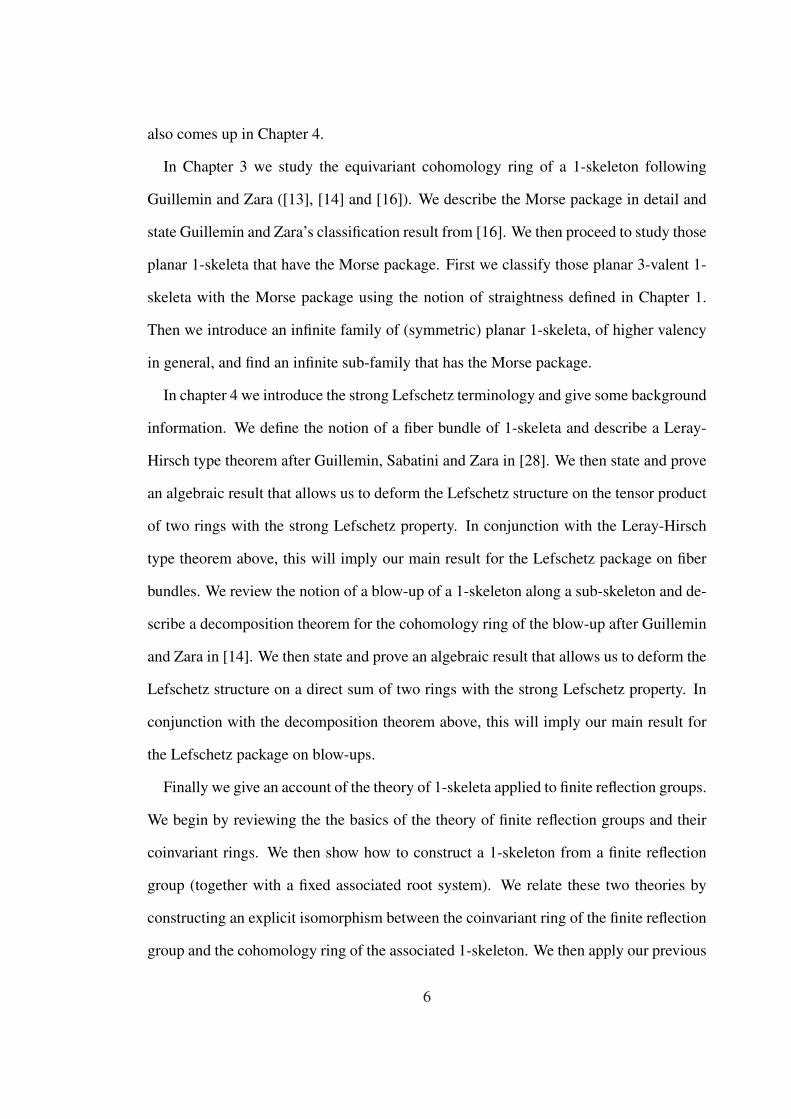
The 1-skeleton in Figure 2 is the 1-skeleton of a polygon in R2. We will see in Chapter

2 that in general, any simple d-polytope in Rd gives a d-valent 1-skeleton in Rd.

Figure 2. a polygon

13

In fact the axioms in Definition 1.1.2 are flexible enough to also allow for certain

projections of 1-skeleta. In Figure 3 we have a 1-skeleton in R3 that is a projection of

a deformed hyper-cube in R4. We will have more to say about 1-skeleta of projected

simple polytopes in Chapter 2 as well.

Figure 3. projected simple polytope

In some special cases certain other polytopes give rise to 1-skeleta. For instance in

Figure 4 we see the 1-skeleton of what appears to be a 3-dimensional octahedron. In

order to satisfy A3 in Definition 1.1.2 it is necessary that the four vertices in the “equato-

rial belt” lie in the same 2-plane. Hence the vertices of the octahedron must be in special

position.

Moving away from polytopes we look at some other planar 1-skeleta. For instance in

Figure 5 we see a 3-valent 1-skeleton in R2 whose underlying graph Γ is actually planar

(when we speak of a planar 1-skeleton we mean a 1-skeleton in R2, whereas a planar

graph is a graph that can be embedded in the plane in the topological sense). Those

readers who are familiar with Steinitz’ theorem (see the concluding remarks in chapter

2) will note right away that this is not the 1-skeleton of a projected simple polytope.

The 1-skeleton in Figure 6 is part of a larger family of 1-skeleta arising from finite

reflection groups; this one comes from the symmetric group S 3. The finite reflection

14

Figure 4. octahedron in special position

Figure 5. 3-valent planar 1-skeleton

group (S 3 in this case) acts on the 1-skeleton via reflection through the edges. We will

discuss this class of 1-skeleta in more detail in Chapter 4.

Figure 6. 1-skeleton of finite reflection group S 3

Another type of planar 1-skeleta that is related to the one shown in Figure 6 is shown

in Figure 7. This 1-skeleton also comes with a finite reflection group generated by re-

flections through the edges. The 1-skeleton in Figure 7 is part of the larger family of

crossed-regular polygons which we will meet formally in Chapter 3.

15

Figure 7. crossed-regular polygon

The non-convex quadralateral shown in Figure 8 is not a 1-skeleton. More precisely,

there is no axial function for this particular embedded graph. We have illustrated a

possible attempt to define an axial function using axioms A2 and A3 in Definition 1.1.2:

the reader can see where the attempt will fail.

Figure 8. a non-convex polygon is not a 1-skeleton

Finally we give an illustration of the concept of an embedding. Figure 9 shows two

“drawings” of the same 1-skeleton. The first drawing is an embedding while the second

is not. We have indicated the axial function on each graph for emphasis.

This concludes the guided tour.

16

ab

c d cd

ab

Figure 9. an embedding

1.3 Sub-skeleta, Holonomy and Straightness

Fix a d-valent 1-skeleton with connection (Γ, α, θ) ⊂ Rn.

Let Γ0 = (V0, E0) be a connected k-valent sub-graph. We say that Γ0 is the graph of a

sub-skeleton of Γ if the restriction of α to E0,

α0 B α|E0 : E0 → Rn

is an axial function on Γ0; we write (Γ0, α0) ⊂ (Γ, α) in this case. For each p ∈ VΓ0 set

E0p ⊂ Ep to be those edges at p that lie in Γ0 and set N0

p = Ep \ E0p to be the normal edges

to Γ0 at p. We set

N0 B⋃

p∈VΓ0

N0p.

If θ = {θe}e∈EΓis a connection on Γ and

θe(E0i(e)) ⊂ E0

t(e)

for each e ∈ E0 then we can restrict θ to Γ0 to get a connection

θ0 = {(θ0)e B (θe)|E0i(e)}e∈E0

on Γ0 for which α0 is compatible. In this case Γ0 is the graph of a totally geodesic sub-

skeleton of Γ and we write (Γ0, α0, θ0) ⊂ (Γ, α, θ). Note in this case there are also induced

maps on the normal edges θ⊥e : N0i(e) → N0

t(e) for each e ∈ E0.

17

(Γ, α, θ) always admits a certain class of totally geodesic sub-skeleta called k-slices

that are gotten as follows. For each sub-space H ⊂ Rn we define the sub-graph ΓH =

(VH, EH) ⊂ Γ by defining

EH B {e ∈ EΓ | α(e) ∈ H}

and

VH B {v ∈ VΓ | v = i(e) for some e ∈ EH} .

We will denote by Γ0H = (V0

H, E0H) ⊂ ΓH ⊂ Γ any connected component of ΓH.

Theorem 1.3.1. The sub-graph Γ0H has constant valency and is the graph of a totally

geodesic sub-skeleton (Γ0H, α

0H, θ

0H) of (Γ, α, θ).

Proof. Fix e B pq ∈ E0H. We need to show that θe((E0

H)p) = (E0H)q. Let e′ ∈ (E0

H)p

be any oriented edge at p different from e. Then α(θe(e′)) must lie in the 2-plane

spanR{α(e), α(e′)} by A3 in Definition 1.1.2. Since α(e) and α(e′) both lie in the sub-

space H, α(θe(e′)) must also lie in H. Conversely let e′ ∈ Ep \ (E0H)p be any oriented edge

at p not in Γ0H. Then the 2-plane spanR{α(e), α(e′)} intersects H in the line spanned by

α(e). If α(θe(e′)) lies in H then it must be collinear with α(e). This means that α(θe(e′))

and α(e) must be collinear by A2 in Definition 1.1.2. On the other hand this is impossible

by A1 in Definition 1.1.2. Therefore α(θe(e′)) does not lie in H. �

If dim(H) = k we call (Γ0H, α

0H, θ

0H) a k-slice of (Γ, α, θ). Of particular interest to us in

subsequent chapters will be the 2-slices of a 1-skeleton.

Fix a totally geodesic sub-skeleton (Γ0, α0, θ0). Fix vertices p, q ∈ VΓ. Let

γ : p0 = p � . . . � q = p j

be a path from p to q.

18

Definition 1.3.2. The path-connection map for γ is

Kγ B θp j−1 p j ◦ . . . ◦ θp0 p1 : Ep0 → Ep j .

If γ ⊂ Γ0 the normal path-connection map for γ is

K⊥γ B θ⊥p j−1 p j◦ . . . ◦ θ⊥p0 p1

: N0p0→ N0

p j.

A loop in Γ is a path γ from a vertex p to itself:

γ : p � · · · � p.

Definition 1.3.3. The path-connection map (resp. normal path-connection map) Kγ : Ep →Ep (resp. K⊥γ : N0

p → N0p) for a loop γ : p � · · · � p is called the holonomy map (resp.

normal holonomy map) for γ.

Note that holonomy maps (resp. normal holonomy maps) act as permutations of the

finite sets Ep (resp. N0p). If the permutation is the identity, we say that the holonomy map

(resp. normal holonomy map) is trivial.

Definition 1.3.4. A totally geodesic sub-skeleton (Γ0, α0, θ0) has trivial normal holonomy

if all of the normal holonomy maps K⊥γ are trivial.

The compatibility constants record important information about the 1-skeleton with

connection (Γ, α, θ). The path-connection maps transport edges to edges along paths and

hence give combinatorial information about the structure of the pair (Γ, θ). By examining

how the compatibility constants transport along a path we get geometric information

about the 1-skeleton (Γ, α, θ). This leads to a notion of straightness which will play an

important role in what follows.

Let {λe}e∈EΓbe compatibility constants on (Γ, α, θ).

19

Definition 1.3.5. The path-connection number for γ is

|Kγ| B∏

e∈Ep0

λp0 p1(e)

· · ·

∏

e∈Ep j−1

λp j−1 p j(e)

.

If γ ⊂ Γ0 the normal path-connection number for γ is

|K⊥γ | B∏

e∈N0p0

λp0 p1(e)

· · ·

∏

e∈N0p j−1

λp j−1 p j(e)

.

For each e ∈ Ep the path-connection number for γ at e is

|Kγ(e)| Bj∏

i=1

λpi−1 pi(θpi−2 pi−1 ◦ · · · ◦ θp0 p1(e)).

If γ is a loop, replace the term “path-connection” with “holonomy”.

Definition 1.3.6. Let (Γ, α, θ) be a 1-skeleton and (Γ0, α0, θ0) a totally geodesic sub-

skeleton.

A. The 1-skeleton (Γ, α, θ) is straight if |Kγ| = 1 for every loop γ in Γ.

B. The totally geodesic sub-skeleton (Γ0, α0, θ0) is normally straight in (Γ, α, θ) if |K⊥γ | =1 for every loop γ in Γ0.

C. (Γ0, α0, θ0) is level in (Γ, α, θ) if for each e ∈ N0p and every loop γ in Γ0 such that

Kγ(e) = e, we have |Kγ(e)| = 1.

As we will see in Chapter 3, level implies normally straight. However the converse

does not hold in general. For example consider the 4-valent 1-skeleton (Γ, α) ⊂ R2 shown

in Figure 10. Choose a connection θ = {θe}e∈EΓon (Γ, α) such that the induced subgraph

Γ0 on the vertex set {p, q, r} is totally geodesic and around the edges of Γ0, satisfies

θpq(ppi) = qq1−i,

θpr(ppi) = rr1−i

θqr(qqi) = rri,

20

for i = 0, 1.

Equipped with this connection the sub-skeleton (Γ0, α0, θ0) has trivial normal holon-

omy (i.e. θrp ◦ θqr ◦ θpq(ppi) = ppi, for i = 0, 1) and is normally straight. However

(Γ0, α0, θ0) is not level in this case (the compatibility constants λpq and λpr are identically

1, whereas λqr is not).

Normal straightness is a property of totally geodesic sub-skeleta that is insensitive

to the normal connection, whereas levelness is a more sensitive property that detects

changes in the normal holonomy. In this last example it is possible to choose a different

connection on (Γ, α) such that Γ0 is totally geodesic and level.

1q

1r

p1

r0

q0

0p

q r

p

Figure 10. normally straight, but not level

The following computation will be used throughout this thesis. We state it as a lemma

so we can refer to it later.

Let H ⊂ Rn k-dimensional sub-space and let (Γ0H, α

0H, θ

0H) be a k-slice. Fix p ∈ V0.

Fix an oriented edge e ∈ E0p and an oriented edge e′ ∈ N0

p. Let W ⊂ Rn denote the

k + 1-dimensional subspace spanned by H and α(e′) (note that α(e′) does not lie in H)

and let ηe′ ∈ (W)∗ denote the covector that annihilates H.

Lemma 1.3.7. The compatibility constant λe(e′) satisfies the equation

λe(e′) =〈ηe′ , α(e′)〉〈ηe′ , α(θe(e′))〉 . (1.3.1)

21

Proof. First observe that the constant λe(e′) is uniquely determined by the condition

α(e′) − λe(e′)α(θe(e′)) ∈ spanR{α(e)}. Therefore it suffices to check that

α(e′) − 〈ηe′ , α(e′)〉〈ηe′ , α(θe(e′))〉α(θe(e′)) ∈ spanR{α(e)}. (1.3.2)

The LHS of (1.3.2) is in the 2-plane spanned by α(e) and α(e′) (since α(θe(e′)) is) and

the LHS is also in the k-plane H (since H is the subspace of W characterized by the

vanishing of ηe). But these two sub-spaces meet only in the one dimensional linear sub-

space spanR{α(e)} hence equation (1.3.2) must hold and this proves the lemma. �

Lemma 1.3.7 implies that the k-slices of a 1-skeleton are always level.

Corollary 1.3.8. Every k-slice is level.

Proof. Let γ : p0 � p1 � · · · � pr−1 � p0 be a loop in Γ0H. Then

|Kγ(e′)| =r−1∏

i=0

λpi pi+1(θpi−1 pi ◦ · · · ◦ θp0 p1(e′)) =

〈η0e′ , α(e′)〉

〈η0e′ , α(Kγ(e′))〉

.

In particular if Kγ(e′) = e′, then |Kγ(e′)| = 1. This shows that the k-slice (Γ0, α0, θ0) is

level. �

1.4 Polarizations

Fix a d-valent 1-skeleton with connection (Γ, α, θ) ⊂ Rn.

An orientation of Γ is a choice of one oriented edge for each pair {e, e} ⊂ EΓ; this

chosen oriented edge is called the directed edge. A path

γ : p � · · · � q

is said to be oriented (with respect to the orientation on Γ) if pi pi+1 is a directed edge.

The orientation is called acyclic if there are no oriented loops.

22

A covector ξ ∈ (Rn)∗ is generic with respect to the pair (Γ, α) if 〈ξ, α(e)〉 , 0 for each

edge e ∈ EΓ where 〈ξ, x〉 denotes the dual pairing of ξ ∈ (Rn)∗ with x ∈ Rn. A generic

covector ξ for Γ induces an orientation on Γ by declaring e ∈ EΓ to be a directed edge if

and only if 〈ξ, α(e)〉 > 0.

Definition 1.4.1. The generic covector ξ is called polarizing if the induced orientation

on Γ is acyclic. If there is a polarizing covector ξ for the pair (Γ, α) then we say that the

1-skeleton (Γ, α) ⊂ Rn admits a polarization or that (Γ, α) ⊂ Rn is polarized by ξ.

Remark. In [14], Guillemin and Zara use the term “polarizing” to describe what we

call “generic” and what we call a “polarizing covector” they call a “polarizing covector

satisfying the ‘no-cycle condition’”.

A 1-skeleton need not admit any polarization at all. For example the 3-valent 1-

skeleton shown in Figure 11 does not admit any polarization. In this example the axial

function value at each oriented edge is assumed to lie on the line segment representing

the edge and to point from the initial vertex to the terminal vertex except at the two inner

edges where we have indicated the “corrected” assignment with arrows. See [14] for

another example coming from geometry.

Figure 11. no polarization

23

On the other hand if a 1-skeleton admits an embedding, then every generic covector

ξ ∈ (Rn)∗ is polarizing. We state this formally as a lemma because we will appeal to this

fact later. Guillemin and Zara also make this observation in [13].

Lemma 1.4.2. If (Γ, α) ⊂ Rn has an embedding then every generic covector ξ for (Γ, α)

is polarizing.

Proof. Let ξ ∈ (Rn)∗ be a generic covector for (Γ, α) ⊂ Rn and let f : VΓ → Rn be an

embedding for (Γ, α). Suppose that

γ : p0 � · · · � pn � p0

is an oriented loop with respect to the orientation induced by ξ. Then we have

0 < 〈ξ, α(pi pi+1)〉

for 0 ≤ i ≤ n. Since f is an embedding we get the string of inequalities

〈ξ, f (p0)〉 < 〈ξ, f (p1)〉 < · · · < 〈ξ, f (pn)〉 < 〈ξ, f (p0)〉,

which is a contradiction. Hence there are no oriented loops in the orientation induced by

ξ hence ξ is polarizing. �

Definition 1.4.3. ([14]) Given a polarizing vector ξ ∈ (Rn)∗ for (Γ, α) we say an injective

function φ : VΓ → R is a Morse function on (Γ, α) compatible with ξ if for each edge

pq ∈ EΓ satisfying 〈ξ, α(pq)〉 > 0 we have φ(p) < φ(q).

Remark. As pointed out in [14], the existence of a polarizing vector guarantees the

existence of a compatible Morse function. Indeed just define φ(v) to be the length of the

longest oriented path in Γ that starts at v. This is well defined since there are no oriented

loops. We can then perturb φ a little to make it injective.

24

Definition 1.4.4. ([14]) For p ∈ VΓ define the index of v (with respect to a generic

covector ξ) to be the number of oriented edges “directed into” v; in other words

indξ(p) B #{e ∈ Ep | 〈ξ, α(e)〉 < 0}.

Define the ith combinatorial Betti number of Γ by

bi(Γ, α) B #{p ∈ VΓ | indξ(p) = i}.

While the index of a vertex of Γ clearly depends on the generic covector, ξ, a theorem

of Bolker implies that the combinatorial Betti numbers are actually independent of ξ.

Theorem 1.4.5. The numbers bi(Γ, α) are independent of the generic covector ξ.

Proof. The set of direction vectors {α(e) | e ∈ EΓ} ⊂ Rn divide (Rn)∗ into cones, the walls

of which are the annihilators of the α(e)’s. The idea is then to examine what happens to

the combinatorial Betti numbers of (Γ, α) as one passes from one cone to a neighboring

one. For more details, see [14], Theorem 1.3.1. �

1.5 Cohomology Rings

In this subsection we introduce two (related) rings associated to a 1-skeleton that will

play a central role in this thesis (in particular Chapters 3 and 4).

Fix a d-valent 1-skeleton with connection (Γ, α, θ) ⊂ Rn. Let S B Sym(Rn) denote the

symmetric algebra of Rn or, equivalently, the ring of polynomial functions on (Rn)∗. Let

Maps(VΓ, S ) �⊕

p∈VΓ

S .

Maps(VΓ, S ) is a graded ring where multiplication is component-wise.

For any subset I ⊂ S , let 〈I〉 ⊂ S denote the ideal generated by I.

25

Definition 1.5.1. The equivariant cohomology ring of (Γ, α) ⊂ Rn is the subring

H(Γ, α) B { f : VΓ → S | f (p) − f (q) ∈ 〈α(pq)〉 for each pq ∈ EΓ} .

We let Hi(Γ, α) denote the ith graded piece of H(Γ, α). The polynomial ring S includes

in H(Γ, α) as the constant functions, giving H(Γ, α) the structure of a graded S -algebra.

We will discuss sufficient conditions for H(Γ, α) to be a free S -module in chapter 3; in

fact this is one of the motivating questions for the work in Chapter 3.

Let S + ⊂ S denote the ideal generated by polynomials of positive degree.

Definition 1.5.2. The (ordinary) cohomology ring is the quotient ring

H(Γ, α) B(H(Γ, α)/S + · H(Γ, α)

).

We will often use the identity

H(Γ, α) � H(Γ, α) ⊗S S/S + = H(Γ, α) ⊗S R. (1.5.1)

We will refer to an element of the equivariant (resp. ordinary) cohomology ring of a 1-

skeleton as an equivariant class (resp. ordinary class) (when it is clear from the context

we may drop the prefix and just say class).

The support of an equivariant class f ∈ H(Γ, α) is defined to be the set of vertices of

the graph Γ on which the function f is non-zero; i.e. supp( f ) B {p ∈ VΓ | f (p) , 0}.One example of an equivariant class (in degree 1) that we have already encountered is

an embedding of a 1-skeleton. See Figure 12.

We will often be interested in classes whose support is a sub-skeleton.

Definition 1.5.3. A Thom class for a k-valent sub-skeleton (Γ0, α0) ⊂ (Γ, α) is a non-zero

homogeneous equivariant class f ∈ Hd−k(Γ, α) such that supp( f ) ⊂ Γ0.

Not every sub-skeleton admits a Thom class; this is related to normal straight-ness;

see Chapter 3, Proposition 3.1.7.

26

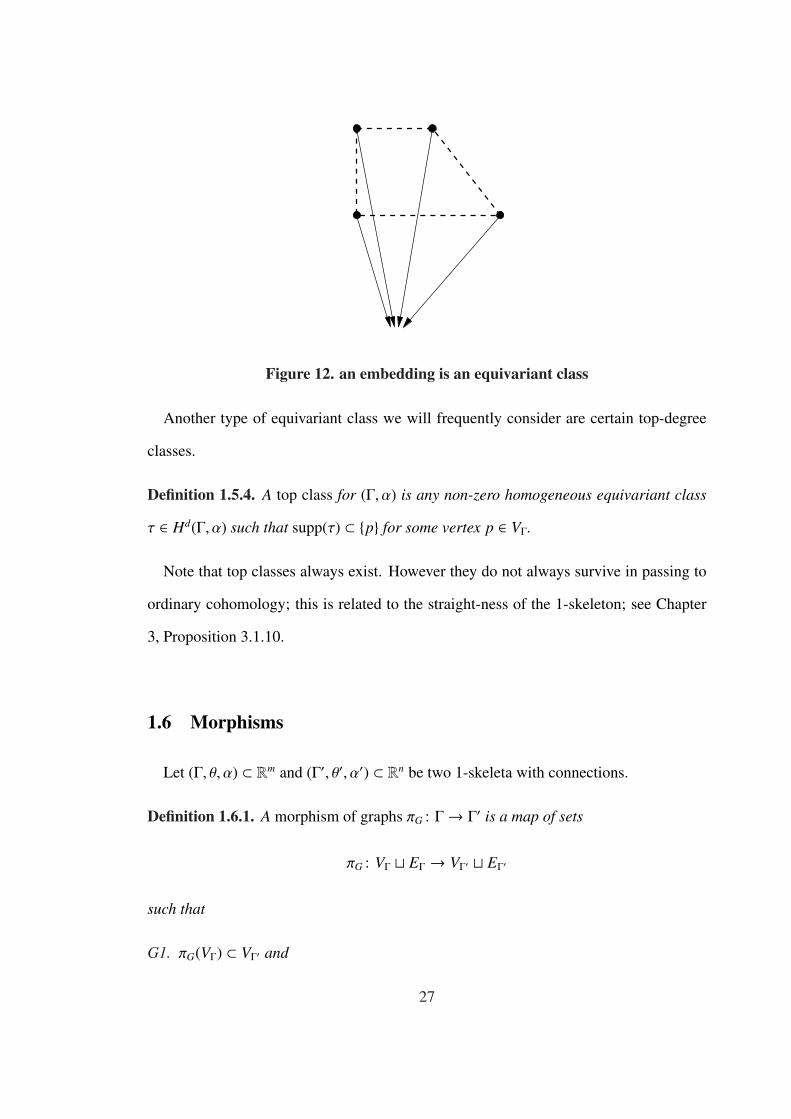
Figure 12. an embedding is an equivariant class

Another type of equivariant class we will frequently consider are certain top-degree

classes.

Definition 1.5.4. A top class for (Γ, α) is any non-zero homogeneous equivariant class

τ ∈ Hd(Γ, α) such that supp(τ) ⊂ {p} for some vertex p ∈ VΓ.

Note that top classes always exist. However they do not always survive in passing to

ordinary cohomology; this is related to the straight-ness of the 1-skeleton; see Chapter

3, Proposition 3.1.10.

1.6 Morphisms

Let (Γ, θ, α) ⊂ Rm and (Γ′, θ′, α′) ⊂ Rn be two 1-skeleta with connections.

Definition 1.6.1. A morphism of graphs πG : Γ→ Γ′ is a map of sets

πG : VΓ t EΓ → VΓ′ t EΓ′

such that

G1. πG(VΓ) ⊂ VΓ′ and

27

G2.

πG(pq) =

π(p)π(q) if π(p) , π(q)

π(p) if π(p) = π(q)(1.6.1)

We say that πG : (Γ, θ) → (Γ′, θ′) is a morphism of graph-connection pairs if in addition

to G1 and G2 we also have

G3. for each e, e ∈ π−1G (EΓ′) ∩ Ep we have that

θe(e) ∈ π−1G (EΓ′)

and

πG(θe(e)) = θ′πG(e)(πG(e)).

Set

Eh B π−1G (EΓ′) ⊂ EΓ;

we call this the set of horizontal edges of Γ (with respect to πG). Set

Ev B π−1G (VΓ′) ∩ EΓ;

we call this the set of vertical edges of Γ (with respect to πG). For each vertex p ∈ VΓ

we denote by Ehp the horizontal edges at p and Ev

p denotes the vertical edges at p. The

morphism of graphs πG restricts to give a map of edge sets

πG : Eh → EΓ′ ,

and for each vertex p ∈ VΓ

πG,p : Ehp → E′πG(p).

Definition 1.6.2. A morphism of 1-skeleta (with connection) is a pair

π B (πG, πL) : (Γ, α, θ)→ (Γ′, α′, θ′)

28

where πG is a morphism of graphs (with connection) and πL is a linear map (in the

opposite direction) that makes the diagram commute

Rm RnπLoo

π−1G (EΓ′) πG

//

α

OO

EΓ′ .

α′

OO

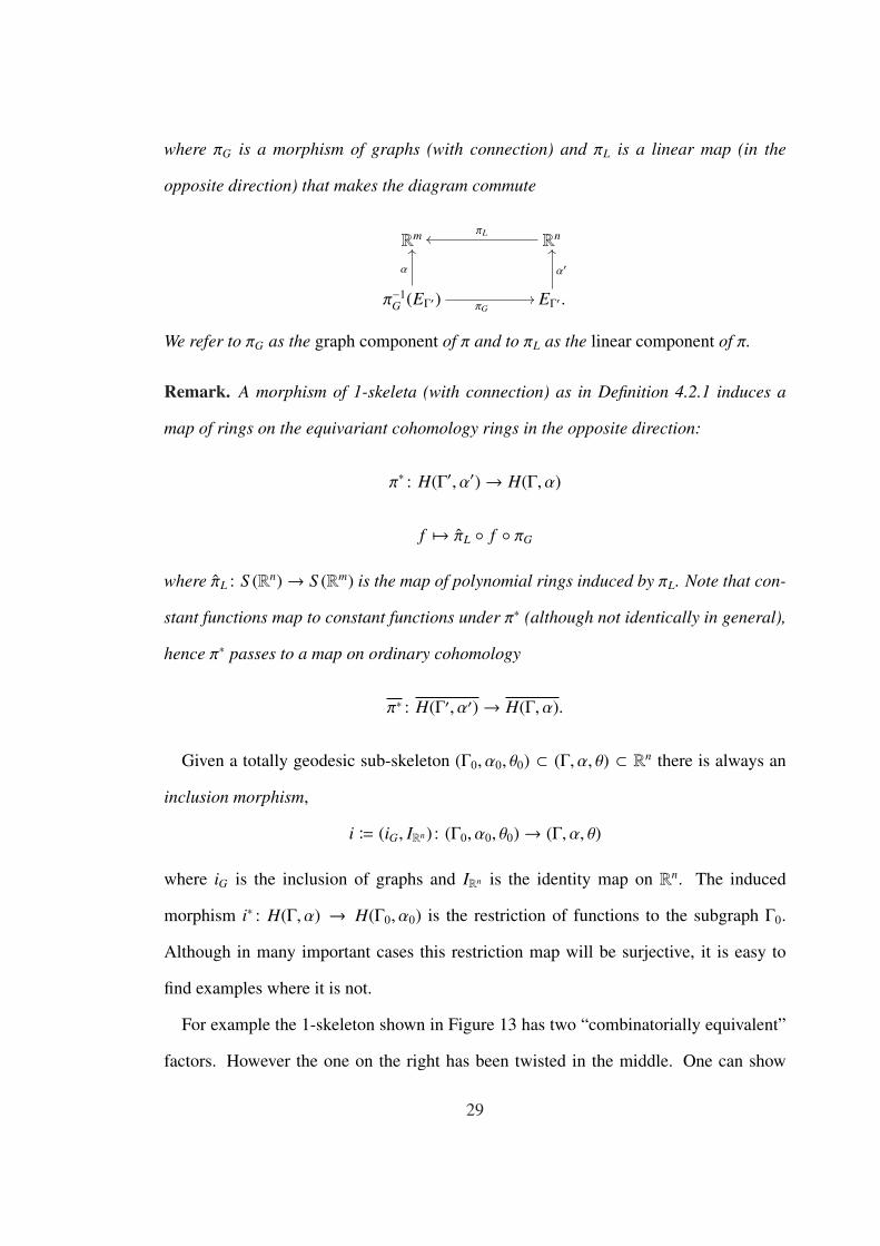
We refer to πG as the graph component of π and to πL as the linear component of π.

Remark. A morphism of 1-skeleta (with connection) as in Definition 4.2.1 induces a

map of rings on the equivariant cohomology rings in the opposite direction:

π∗ : H(Γ′, α′)→ H(Γ, α)

f 7→ πL ◦ f ◦ πG

where πL : S (Rn)→ S (Rm) is the map of polynomial rings induced by πL. Note that con-

stant functions map to constant functions under π∗ (although not identically in general),

hence π∗ passes to a map on ordinary cohomology

π∗ : H(Γ′, α′)→ H(Γ, α).

Given a totally geodesic sub-skeleton (Γ0, α0, θ0) ⊂ (Γ, α, θ) ⊂ Rn there is always an

inclusion morphism,

i B (iG, IRn) : (Γ0, α0, θ0)→ (Γ, α, θ)

where iG is the inclusion of graphs and IRn is the identity map on Rn. The induced

morphism i∗ : H(Γ, α) → H(Γ0, α0) is the restriction of functions to the subgraph Γ0.

Although in many important cases this restriction map will be surjective, it is easy to

find examples where it is not.

For example the 1-skeleton shown in Figure 13 has two “combinatorially equivalent”

factors. However the one on the right has been twisted in the middle. One can show

29

directly that while the factor on the left supports a Thom class on its upper triangle, the

factor on the right does not. Hence it is impossible to extend this Thom class on the

right factor to a global class on the entire 1-skeleton. We have illustrated in the figure

an attempt to extend such a class; the arrows and 0’s are the desired values of the class

at the vertices and the question marks indicate where we get stuck. The 1-skeleton in

Figure 13 is an example of a pseudo-fiber bundle of 1-skeleta (see Chapter 4, Definition

4.2.5).

00

0 0

00

?

?

?

Figure 13. restriction to the left factor is not surjective

1.7 1-skeleta in Nature

In this section we define a class of smooth manifolds admitting compact torus actions

called GKM T -manifolds. We then show how one obtains a 1-skeleton from a GKM

T -manifold.

Let M be a 2d-dimensional compact smooth manifold. A 2-form on M is a smooth

section

ω : M → ∧2T ∗M,

30

or equivalently a family of alternating, R-bilinear forms

ωp : TpM × TpM → R

varying smoothly with p ∈ M.

A metric g on M is a smooth positive definite section

g : M → S 2(T ∗M),

or equivalently a family of symmetric, positive definite R-bilinear forms

gp : TpM × TpM → R

varying smoothly with p ∈ M.

Let T = (S 1)n be a compact n-dimensional torus acting smoothly on M. Let ψt : M →M denote the diffeomorphism corresponding to t ∈ T . Suppose the T action is effective

(i.e. T 3 t 7→ ψt ∈ Diff(M) is an injective group homomorphism).

We say that a smoothly varying R-bilinear form Θ : TpM × TpM → R is T-invariant

if

Θψt(p)((ψt)∗X, (ψt)∗Y) = Θp(X,Y)

for every p ∈ M and every X,Y ∈ TpM.

A fundamental fact from differential geometry states that every manifold M admits a

metric g. We also have the following fact.

Theorem 1.7.1. Let T be a compact Lie group acting smoothly on a manifold M. Then

there is a metric g on M that is T-invariant.

Proof. Since T is compact, we can average any fixed metric g over T to get a new metric

that is T -invariant. See [19] Theorem 2.39 for the details. �

Fix a T -invariant metric g on M. Assume that M admits a non-degenerate T -invariant

2-form ω.

31

Definition 1.7.2. An almost complex structure on M is a smooth section J : M → Aut(T M)

such that J2 = −I.

A. We say that J is compatible with ω if

(a) ωp(X, Jp(X)) ≥ 0 for each p ∈ M and for all non-zero vectors X ∈ Tp(M)

(b) ωp(Jp(X), Jp(Y)) = ωp(X,Y) for each p ∈ M and for all vectors X,Y ∈ Tp(M).

B. We say that J is compatible with the metric g if

gp(Jp(X), Jp(Y)) = gp(X,Y)

for each p ∈ M and for all vectors X,Y ∈ Tp(M).

C. We say that J is T-invariant if Jψt(p)((ψt)∗X) = (ψt)∗(Jp(X)) for all p ∈ M and X ∈TpM.

Lemma 1.7.3. M admits a T-invariant almost complex structure J that is compatible

with ω and g.

Proof. See [21] Proposition 2.61. �

Let us fix a T -invariant almost complex structure J on M that is compatible with ω

and g as in Lemma 1.7.3.

Let MT denote the T -fixed point set of M and let p ∈ MT . There is a linear action of

T on TpM by

(ψt)∗ : TpM → TpM.

Using J we can view TpM as a vector space over C by the formula

(x + iy)U B xU + yJ(U).

32

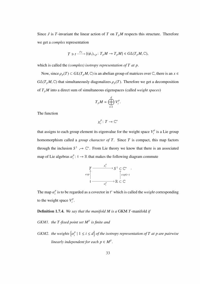
Since J is T -invariant the linear action of T on TpM respects this structure. Therefore

we get a complex representation

T 3 tρp

// {(ψt)∗,p : TpM → TpM} ∈ GL(TpM,C),

which is called the (complex) isotropy representation of T at p.

Now, since ρp(T ) ⊂ GL(TpM,C) is an abelian group of matrices over C, there is an x ∈GL(TpM,C) that simultaneously diagonalizes ρp(T ). Therefore we get a decomposition

of TpM into a direct sum of simultaneous eigenspaces (called weight spaces)

TpM 'd⊕

i=1

V pi .

The function

χpi : T → C∗

that assigns to each group element its eigenvalue for the weight space V pi is a Lie group

homomorphism called a group character of T . Since T is compact, this map factors

through the inclusion S 1 ↪→ C∗. From Lie theory we know that there is an associated

map of Lie algebras αpi : t→ R that makes the following diagram commute

Tχ

pi // S 1 ⊂ C∗

tα

pi

//

exp

OO

R ⊂ Cexp(i−)

OO.

The map αpi is to be regarded as a covector in t∗ which is called the weight corresponding

to the weight space V pi .

Definition 1.7.4. We say that the manifold M is a GKM T -manifold if

GKM1. the T-fixed point set MT is finite and

GKM2. the weights{α

pi | 1 ≤ i ≤ d

}of the isotropy representation of T at p are pairwise

linearly independent for each p ∈ MT .

33

Suppose M is a GKM T -manifold. For each p ∈ MT and each character χpi let

ker(χpi ) C K p

i ⊂ T ; K pi is a codimension one compact subgroup of T . Now restrict

the T action on M to K pi and let Xp

i ⊂ M denote the connected component of the fixed

point set MK pi ⊂ M containing p. We have the following general theorems from the

theory of transformation groups. We refer the reader to Kawakubo’s book [19] for the

proofs.

Theorem 1.7.5. For each x ∈ Xpi there exists a K p

i -invariant open neighborhood U ⊂ M

of x and a K pi -equivariant diffeomorphism

φ : TxM → U

(with respect to the isotropy representation of K pi at x).

Proof. See [19] Theorem 4.8. �

Armed with Theorem 1.7.5 one can also prove

Theorem 1.7.6. Let K be a compact Lie group acting smoothly on a manifold M, and

let XK ⊂ M be the fixed point set of M. Then XK is a closed embedded sub-manifold of

M.

Proof. See [19] Theorem 4.14. �

Hence by Theorem 1.7.6 Xpi ⊂ M is a closed (hence compact since M is compact)

embedded sub-manifold of M. By Theorem 1.7.5 the tangent space Tp(Xpi ) ⊂ TpM at

p ∈ Xpi is exactly the sub-space that is fixed point-wise by the (linear) action of K p

i . By

GKM 2 we conclude that TpXpi is precisely the weight space V p

i . In particular we see

that Xpi is a compact, connected sub-manifold of (real) dimension 2.

34

Furthermore, since the complex structure J is compatible with ω we get that ω|Xpi

is

non-degenerate. Hence Xpi is orientable. Since K p

i is the sub-group that fixes Xpi point-

wise there is an effective action of the quotient group T/K pi � S 1 on Xp

i . Fortunately

effective S 1 actions on compact connected surfaces are completely understood.

Theorem 1.7.7. If X is a compact, connected, orientable surface with an effective S 1

action with fixed points, then X is S 1-equivariantly diffeomorphic to S 2 with the standard

S 1 action.

Proof. See [1] Section 3.1. �

Therefore Xpi is an embedded T -invariant S 2 with exactly two fixed points p, q ∈ MT .

We are now in a position to show how to associate a d-valent 1-skeleton in t∗ � Rn to

the 2d-dimensional GKM T -manifold M.

Define a graph Γ = (VΓ, EΓ) where VΓ B MT and EΓ is the set of (oriented) embedded

T -invariant S 2’s described above. This graph is 12 dim(M) = d-valent from our discussion

above.

There is a natural function α : EΓ → t∗ defined by

EΓ 3 Xpi

α // αpi ∈ t∗.

Now we need to show that this is an axial function on Γ.

By GKM2 in Definition 1.7.4, A1 from Definition 1.1.2 holds. It follows from Theo-

rem 1.7.7 that A2 holds for α. To see that A3 holds requires a little more effort.

Let us first cook up a connection on Γ. Fix p, q ∈ MT and suppose X ⊂ M is the

T -invariant S 2 containing p and q. Let α(pq) ∈ t∗ denote the weight for X and let H ⊂ T

denote the codimension 1 sub-torus whose Lie algebra is ker(α(pq)) ⊂ t. Let T M denote

the tangent bundle of M, T M|X the tangent bundle of M restricted to X and νX the normal

bundle to X ⊂ M. We have the following result, the proof of which is due to Klyachko

and can be found in [20].

35

Proposition 1.7.8. The normal bundle splits T -equivariantly into a direct sum of line

bundles

νX �d−1⊕

i=1

LXi .

Proof. Essentially Klyachko shows that νX decomposes in the usual sense if and only if

it decomposes T -equivariantly. See [20] Theorem 1.2.3 and Proposition 1.2.5. The fact

that νX decomposes into a direct sum of line bundles (in the usual sense) follows from

a more general theorem of Grothendieck that any (holomorphic) complex vector bundle

over a projective line splits. See [25] Theorem 2.1.1. That any smooth complex vector

bundle over S 2 has a holomorphic structure follows from the classification of complex

vector bundles. See the discussion in [4] starting on page 297, and the discussion in [25]

starting on page 111. �

This T equivariant splitting gives rise to natural maps

θpq : Ep → Eq

by defining θpq(Y) = Y ′ where if Y is the T -invariant S 2 containing p whose tangent

space at p is (LXi )p, then Y ′ is the T -invariant S 2 containing q whose tangent space at q

is (LXi )q. This defines a connection on Γ.

Finally, to see that A3 holds it suffices to see that (νX)p is H-equivariantly isomorphic

to (νX)q. Indeed if Υpq : (νX)p → (νX)q is an H equivariant isomorphism and Y is a

generator of weight space at p corresponding to weight αpi then we have

Υpq((ψt)∗,pY) = χpi (t) · Υ(Y) = χ

qi (t)Υ(Y) = (ψt)∗,qΥpq(Y).

Hence we see that χpi |H = χ

qi |H or equivalently that

(αpi − αq

i )|ker(α(pq)) = 0

which is precisely the content of A3 in Definition 1.1.2.

The following corollary of Proposition 1.7.8 answers this call.

36

Corollary 1.7.9. Given any two points p, q ∈ X, there is a H-equivariant linear isomor-

phism

Υpq : (νX)p → (νX)q.

Proof. Let {Vα}α∈Λ be an open cover of X over which the normal bundle is trivial and let{gαβ

}α,β∈Λ be the transition functions. By Proposition 1.7.8, the maps

{gαβ

}α,β∈Λ must be

H-equivariant.

Since X is connected, it suffices to prove the assertion in the case where p ∈ Vβ, q ∈ Vα,

and Vα ∩ Vβ , ∅. In this case we fix z ∈ Vα ∩ Vβ and simply define

(νX)pΥpq

// (νX)q

(p, v) // (q, gαβ(z)(v)).

Then Υpq is H-equivariant since gαβ is. �

Thus A3 holds for α and the triple (Γ, α, θ) is a 1-skeleton with connection in the sense

of Definition 1.1.2. This 1-skeleton with connection is the associated 1-skeleton with

connection for the GKM T -manifold M. If a 1-skeleton with connection arises from a

GKM T -manifold M we will call M an underlying manifold for the 1-skeleton. Notice

that the compatibility constants for (Γ, α, θ) in this case are all equal to 1 hence the 1-

skeleton with connection is GKM in the sense of Remark 1.

Remark. The connection on Γ is not canonical. However, the normal bundle always

admits a canonical H-equivariant splitting into “weight sub-bundles”. If the weights

of the isotropy representation at each fixed point are 3-independent, then these weight

sub-bundles are necessarily line bundles; hence in this case the splitting is canonical.

37

C H A P T E R 2

PROJECTIONS AND LIFTING

There is a projection operation on 1-skeleta that takes as its input a 1-skeleton in RN

and produces a 1-skeleton in Rn for n < N. One can try to go backwards by asking if a

given a 1-skeleton in Rn is a projection of a 1-skeleton in RN for some N > n. This seems

to be a very difficult question to answer in general. In specializing to the case N = d

however, the situation becomes easier to understand.

A particularly nice class of d-valent d-independent 1-skeleta are those coming from

simple d-polytopes in Rd, or more generally, those coming from complete simplicial fans

in (Rd)∗. In [14], Guillemin and Zara defined the notion of a non-cyclic 1-skeleton for

the 3-independent case. It turns out that the non-cyclic 1-skeleta in the d-independent

case are exactly those coming from complete simplicial fans in (Rd)∗. The main result

of this chapter is a characterization of those 1-skeleta which are projections of d-valent,

d-independent non-cyclic 1-skeleta.

One of the main tools we use is a beautiful operation called reduction due to Guillemin

and Zara. The class of 1-skeleta on which this operation can be performed is called re-

ducible (in the 3-independent case, reducible and non-cyclic coincide). For 3-independent

1-skeleta, the reduction operation takes as its input a reducible d-valent 1-skeleton in Rn

and its output is a (d − 1)-valent 1-skeleton in Rn−1, called a cross-section. For gen-

eral 1-skeleta (i.e. not 3-independent) the reduction operation takes a reducible d-valent

38

1-skeleton in Rn and produces a (d − 1)-valent generalized 1-skeleton in Rn−1.

A d-valent, d-independent non-cyclic 1-skeleton is reducible and any projection of it is

also reducible. Moreover the cross-sections of the projection coincide with the projection

of the cross-sections. We will show that the converse holds as well: If the cross-sections

of a d-valent reducible 1-skeleton in Rn lift, then the 1-skeleton itself lifts to a d-valent

d-independent non-cyclic 1-skeleton in Rd.

This chapter is divided into five sections. In Section 1 we introduce the general lifting

problem and we introduce and discuss the important class of 1-skeleta coming from

simple polytopes. In Section 2 we define the reducible 1-skeleta (with connections)

and describe the reduction operation, introducing the notions of a pre 1-skeleton and a

generalized 1-skeleton along the way. In Section 3 we introduce the important blow-

up construction (also due to Guillemin and Zara) as well as a couple of other useful

constructions. In Section 4 we put it all together in order to state and prove the main

result. In Section 5 we give some concluding remarks.

2.1 Projections, Simple Polytopes, and a Lifting Problem

In this section we will define the projection operation and state the general lifting prob-

lem. We then give a somewhat lengthy discussion of the class of 1-skeleta arising from

simple polytopes. Finally we will specialize our lifting problem using simple polytopes

as a prototypical model.

2.1.1 Projections

Fix a 1-skeleton with connection (Γ, A, θ) ⊂ RN .

Let p : RN → Rn be a surjective linear map and let Gr(k,N) denote the set of k-

39

dimensional sub-spaces of RN . Define the finite subset

H B{H ∈ Gr(2,N) | Γ0

H ⊂ Γ has valency ≥ 2}.

The map p is generic for (Γ, A) ⊂ RN if dim(π(H)) = 2 for each H ∈ H . In other words,

the projection p is generic for (Γ, A) if p preserves the 2-slices of (Γ, A).

Given a generic projection p : RN → Rn for (Γ, A) we can define a new 1-skeleton by

simply pulling back A by p; that is (Γ, p ◦ A). The generic property of p guarantees that

(A1) of Definition 1.1.2 is satisfied. The linearity of p guarantees that (A2) and (A3) of

Definition 1.1.2 hold; in fact p ◦ A is also compatible with θ with the same compatibility

constants.

Definition 2.1.1. The 1-skeleton with connection (Γ, p◦A, θ) ⊂ Rn is called the projection

of (Γ, A, θ) (with respect to the generic projection p).

Remarks. i. It is useful to remember the connection when projecting a 1-skeleton.

In case (Γ, A, θ) ⊂ RN is 3-independent, the connection θ is uniquely determined

by A. On the other hand for a generic projection p : RN → Rn, the axial function

p ◦ A may fail to be 3-independent, hence there may be other connections on Γ for

which p ◦ A is compatible; only one can come from the projection.

ii. Projection defines a morphism of 1-skeleta with connections

π : (Γ, p ◦ A, θ)→ (Γ, A, θ)

whose graph component is the identity and whose linear component is the pro-

jection map p. The induced map on equivariant cohomology π∗ : H(Γ, A) →H(Γ, p ◦ A) is surjective in many important cases.

The general lifting problem is the following.

40

Problem. Under what conditions is a d-valent 1-skeleton with connection (Γ, α, θ) ⊂Rn a projection of a (-n effective) 1-skeleton with connection (Γ, A, θ) ⊂ RN for some

projection p : RN → Rn?

This problem may be quite difficult to solve in this generality. By restricting the class

of 1-skeleta (Γ, A, θ) ⊂ RN that we project, the problem becomes more tractable. In

[14], Guillemin and Zara introduced the notion of a non-cyclic 1-skeleton which plays a

fundamental role in what follows. Here is their definition.

Definition 2.1.2. ([14]) A 1-skeleton (Γ, α) ⊂ Rn is called non-cyclic if the following

conditions hold:

NC1. (Γ, α) ⊂ Rn admits a polarization

NC2. b0(Γ0H, α

0H) = 1 for every 2-slice (Γ0

H, α0H).

In Figure 14, the first 1-skeleton is non-cyclic, while the second is not.

Figure 14. non-cyclic and not non-cyclic

Remarks. i. Note that if (Γ, α) ⊂ R2 then the only 2-slice is the entire 1-skeleton so

NC2 in Definition 2.2.1 reduces to saying that b0(Γ, α) = 1.

ii. In [14], Guillemin and Zara defined this notion for 3-independent 1-skeleta. We

do not require this condition here. In particular we will use this notion in chapter

3 when we discuss planar 1-skeleta.

41

Another specialization we will make on the d-valent 1-skeleton with connection (Γ, A, θ) ⊂RN is by restricting to the extreme case when N = d. Requiring A to be effective in this

case is equivalent to requiring A to be d-independent. This turns out to be a very restric-

tive condition.

An important class of d-valent, d-independent 1-skeleta are those coming from simple

polytopes.

2.1.2 Polytopes and Projected Polytopes

Here we review some basic facts about polytopes and fans. We show how to construct

a 1-skeleton from a simple polytope. The main result of this section is the characteriza-

tion of those 1-skeleta coming from a simplicial fan.

A d-polytope P ⊂ Rd is the convex hull of finitely many points in Rd that affinely

span Rd (hence P ⊂ Rd is necessarily compact). A k-face of P for 0 ≤ k ≤ d is any

k-dimensional subset of P that minimizes some linear functional η : Rd → R restriced to

P. We call the 0-faces of P the vertices of P, the 1-faces of P the edges of P, and the

(d−1)-faces the facets of P. Note that an edge of P is a line segment joining two vertices

of P so it makes sense to speak of the “oriented” edges of P.

Denote the set of vertices of P by VP and the set of oriented edges of P by EP. The

graph of P is ΓP B (VP, EP). Note here that the graph ΓP has a natural embedding in the

sense of Definition 1.1.5 in chapter 1; denote this embedding by

VΓ// Rn

p // ~p.

We say that a d-polytope P ⊂ Rd is simple if ΓP is d-valent. Here are some useful facts

about polytopes that we state as a theorem to be referred to hereafter. We state it without

proof.

42

Theorem 2.1.3. i. Every facet F ⊂ P has associated to it a unique (up to positive

scalar) linear functional ηF : Rd → R such that ηF is minimized on P at F. We call

ηF the inner-normal covector associated to F.

ii. If P is simple, then for any vertex p ∈ VP and for any subset of k edges at p there

is a unique k-face F ⊂ P containing those edges; those edges are said to span F.

iii. If P ⊂ Rd is simple, then the edge directions for (EP)x are a basis for Rd for any

x ∈ VP.

There is a natural function αP : EP → Rd defined using the embedding

αP(pq) B ~q − ~p. (2.1.1)

In the case P ⊂ Rd is simple we can check that αP defines an axial function on ΓP. Indeed,

it is clear from (2.1.1) that A2 of Definition 1.1.2 holds. Item (iii) in Theorem 2.1.3 tells

us that A1 holds. To see that A3 holds, let us first compute the connection θP = {θe}e∈EP

on ΓP. Fix an oriented edge e B pq ∈ (EP)p. For any other oriented edge e′ ∈ (EP)p

there is a unique 2-face Q of P spanned by e, e′, by (ii) in Theorem 2.1.3. Then define

θe(e′) ∈ (EP)q to be the unique oriented edge at q that lies in Q. Then certainly we have

that

α(e′) − λα(θe(e′)) = cα(e) (2.1.2)

for some λ, c ∈ R. It follows from the convexity of Q that λ > 0, and hence θP B

{θe}e∈EP is a connection on ΓP for which αP is compatible. The 1-skeleton with connection

(ΓP, αP, θp) ⊂ Rd is the 1-skeleton associated to the simple polytope P.

We can actually compute these compatibility constants directly. Fix e B pq ∈ (EP)p

as above and let e′ ∈ (EP)p be any other oriented edge at p. By Theorem 2.1.3 (ii),

there is a facet F containing p and e, but not containing e′. Let ηF ∈ (Rd)∗ denote the

inner-normal covector associated to F (which exists by Theorem 2.1.3 (i)). The facet

43

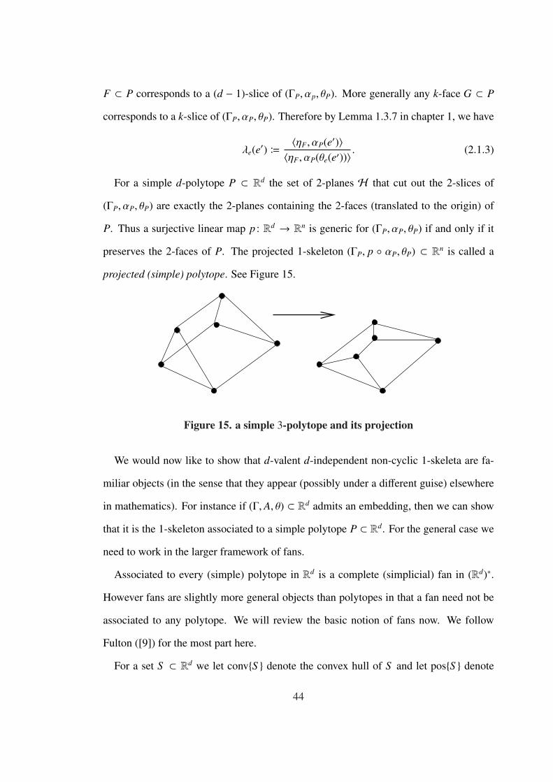
F ⊂ P corresponds to a (d − 1)-slice of (ΓP, αp, θP). More generally any k-face G ⊂ P

corresponds to a k-slice of (ΓP, αP, θP). Therefore by Lemma 1.3.7 in chapter 1, we have

λe(e′) B〈ηF , αP(e′)〉〈ηF , αP(θe(e′))〉 . (2.1.3)

For a simple d-polytope P ⊂ Rd the set of 2-planes H that cut out the 2-slices of

(ΓP, αP, θP) are exactly the 2-planes containing the 2-faces (translated to the origin) of

P. Thus a surjective linear map p : Rd → Rn is generic for (ΓP, αP, θP) if and only if it

preserves the 2-faces of P. The projected 1-skeleton (ΓP, p ◦ αP, θP) ⊂ Rn is called a

projected (simple) polytope. See Figure 15.

Figure 15. a simple 3-polytope and its projection

We would now like to show that d-valent d-independent non-cyclic 1-skeleta are fa-

miliar objects (in the sense that they appear (possibly under a different guise) elsewhere

in mathematics). For instance if (Γ, A, θ) ⊂ Rd admits an embedding, then we can show

that it is the 1-skeleton associated to a simple polytope P ⊂ Rd. For the general case we

need to work in the larger framework of fans.

Associated to every (simple) polytope in Rd is a complete (simplicial) fan in (Rd)∗.

However fans are slightly more general objects than polytopes in that a fan need not be

associated to any polytope. We will review the basic notion of fans now. We follow

Fulton ([9]) for the most part here.

For a set S ⊂ Rd we let conv{S } denote the convex hull of S and let pos{S } denote

44

the set of positive linear combinations of elements of S (the “positive hull”). A convex

polyhedral cone in (Rd)∗ is a subset of the form σ = pos{v1, . . . , vN} B {∑i aivi | ai ≥ 0}for some vi ∈ (Rd)∗. A stictly convex polyhedral cone is a convex polyhedral cone which

does not contain any linear subspace. The cone is i-dimensional if dim(spanR{vi | 1 ≤ i ≤N}) = i and it is simplicial if the generators v1, . . . , vN are linearly independent. Given a

convex polyhedral cone σ define dual σ = {x ∈ Rd | 〈x, y〉 ≥ 0 ∀y ∈ σ}. A face of τ of

σ is the intersection of σ with a supporting hyperplane; i.e. τ = {x ∈ σ | 〈x, u〉 = 0} for

some u ∈ σ. It is straightforward to verify that a face of convex polyhedral cone is again

a convex polyhedral cone.

A fan in (Rd)∗ is any finite collection of convex polyhedral cones {σi}i∈I such that

i. if τ is a face of σ and σ ∈ Σ then τ ∈ Σ,

ii. σi ∩ σ j is a face of both σi and σ j.

Σ is simplicial if every cone is simplicial and it is complete if every v ∈ (Rd)∗ lies in some

cone of Σ. Write |Σ| to be the set {v ∈ (Rd)∗ | v ∈ σ some σ ∈ Σ}. Then Σ is complete if

and only if |Σ| = (Rd)∗. For each i, define Σi to be the set of i dimensional cones in Σ.

A conewise linear function on Σ is a continuous function F : |Σ| → Rwhose restriction

to every cone in Σ is a linear function. Write Fσ for the linear function that F restricts to

on σ. F is called strictly convex if for any two distinct cones σ,σ′ ∈ Σ and any x ∈ σwe have Fσ′(x) > Fσ(x). A complete fan Σ that admits a strictly convex conewise linear

function is called polytopal.

Theorem 2.1.4. Pairs (Σ, F) consisting of a simplicial polytopal (hence complete) fan

Σ ⊂ (Rd)∗ and a strictly convex Σ-conewise linear function F : |Σ| → R are in one-to-one

correspondence with simple d-polytopes P = conv{F|σ | σ ∈ Σd} ⊂ ((Rd)∗)∗ � Rd.

Proof. To go from P to (Σ, F) see [9] page 26, or [29] chapter 7. To go from (Σ, F) to

45

P we need to show that the points {F|σ}σ∈Σd ⊂ ((Rd)∗)∗ � Rd are the vertices of a simple

convex d-polytope.

To see that the points lie in convex position in Rd, we will show that each point Fσ

minimizes a linear functional on the set {F|σ}σ∈Σd and thus also on the set conv{F|σ | σ ∈Σd}. For each σ ∈ Σd choose a covector ξσ which lies in the interior of σ (hence lies

outside every other d-cone in Σ). Then the strict convexity of F implies that for σ′ ∈ Σ

distinct from σ, that 〈ξσ, F|σ′〉 < 〈ξσ, F|σ〉 (unless otherwise stated 〈x, y〉 always denotes

the dual pairing for x ∈ (Rd)∗ and y ∈ Rd). Hence Fσ is minimized by ξσ. Hence the

convex polytope P = conv{F|σ | σ ∈ Σd} has the vertex set {F|σ}σ∈Σd . It is easy to see that

the edges of P are correspond to pairs σ,σ′ ∈ Σd that share a (d − 1) dimensional face

τ: this edge is minimized by a linear functional chosen to lie in the relative interior of τ.

Since Σ is simplicial, every vertex must have exactly d-neighbors (since every cone has

exactly d (d − 1)-dimensional faces). This shows that ΓP is d-valent.

Finally to see that P is a d-polytope (hence simple) we need to show that ifσ0, σ1, . . . , σd ∈Σd are d-cones such that σ0 ∩ σi is a (d − 1) cone and t0, t1, . . . , td ∈ R are weights such

that∑d

i=0 ti = 0 andd∑

i=0

tiFσi = 0, (2.1.4)

then ti = 0 for 0 ≤ i ≤ d (this will show that the (d + 1) points {Fσi | 0 ≤ i ≤ d} are

affinely independent, hence affinely span a d dimensional affine subspace). To see this

choose for each 1 ≤ i ≤ d a linear functional xi that lies on the relative interior of the ray

(i.e. 1-dimensional cone) contained in σ0 but not contained in σ0 ∩σi. Then applying xi

to both sides of (2.1.4) shows that ti is zero. Repeating this argument for all i shows that

ti = 0 for all i. This completes the proof of Theorem 2.1.4. �

The following result shows that a noncyclic d-valent, d-independent 1-skeleton in Rd

gives the same data as a complete simplicial fan in (Rd)∗.

46

Theorem 2.1.5. Let (Γ, A, θ) ⊂ Rd be a d-valent, d-independent non-cyclic 1-skeleton.

Then the set σp B {x ∈ (Rd)∗ | 〈x, A(e)〉 ≥ 0 ∀e ∈ Ep} is a simplicial polyhedral

d-dimensional cone and the set Σ consisting of all the σp (p ∈ VΓ) and all the faces con-

tained therein is a complete simplicial fan. Moreover if (Γ, A) admits an embedding, then

Σ is polyhedral and the embedding provides a strictly convex conewise linear function.

Before proving Theorem 2.1.5, we will need to establish one technical result. For

η ∈ (Rd)∗, let Γη ⊂ Γ be the induced sub-graph on the set of vertices {p ∈ VΓ | 〈η, A(e)〉 ≥0 ∀e ∈ Ep}. Note that e ∈ EΓη if and only if i(e) ∈ VΓη and 〈η, A(e)〉 = 0.

Lemma 2.1.6. Γη ⊂ Γ is connected for all η ∈ (Rd)∗.

Proof. Fix a polarizing covector ξ ∈ (Rd)∗ for (Γ, A). Suppose there is some η ∈ (Rd)∗

such that Γη is not connected. Then there must be two distinct vertices p1, p2 ∈ VΓ

such that 〈ξ, A(e)〉 > 0 for all e ∈(Ep1 ∪ Ep2

)∩ Γη. Indeed just let p1 and p2 be minima

(with respect to the partial order induced from the polarization) on two distinct connected

components of Γη. Thus for M > 0 sufficiently large, the covector ξ = ξ + M · η satisfies

〈ξ, A(e)〉 > 0 for all e ∈(Ep1 ∪ Ep2

). By Theorem 1.4.5, this implies that b0(Γ, A) ≥ 2.

But this is impossible since (Γ, A) is non-cyclic; see Lemma 2.2.5. �

We are now in a position to prove Theorem 2.1.5.

Proof of Theorem 2.1.5. For each p ∈ VΓ and every e ∈ Ep, define the linear functional

Xpe : Rd → R by 〈Xp

e , A(e′)〉 = δee′ for e′ ∈ Ep. It is straightforward to check that

σp = pos{Xpe | e ∈ Ep}. (2.1.5)

which shows that σp is a simplicial polyhedral d-cone.

We would like to see that these cones generate a complete simplicial fan in (Rd)∗.

Hence we need to show that for any two vertices p, q ∈ VΓ, the intersection σp ∩ σq is a

47

face of each of σp and σq. For any pair of vertices p, q ∈ VΓ define the oriented edge sets

Epq B {e ∈ Ep | 〈x, A(e)〉 > 0 some x ∈ σp ∩ σq},

Eqp B {e′ ∈ Eq | 〈x, A(e′)〉 > 0 some x ∈ σp ∩ σq}.

Claim. For each e ∈ Epq there is a unique e′ ∈ Eqp such that Xpe = µXq

e′ for some positve

number µ (depending on p, q and e).

Choose η ∈ (Rd)∗ to be a covector such that 〈η, A(e)〉 > 0 for all e ∈ Epq. By Lemma

2.1.6 the graph Γη is connected. Since η ∈ σp ∩ σq, the vertices p and q must belong to

Γη. Let Wη ⊂ Rd denote the sub-space spanned by edges in Γη; i.e. Wη = spanR{A(e) |e ∈ Γη}. Let γ : p � · · · � q be any path from p to q in Γη. The path-connection map

induces a bijection

Kγ : Epq → Eqp

and we have

A(e) ≡ |Kγ(e)| · A(Kγ(e)) mod Wη. (2.1.6)

Note that for e ∈ Epq and e′ ∈ Eqp, Xpe and Xq

e′ both vanish identically on Wη. Since

Kγ(e) ∈ Eqp, by (2.1.6) we have Xpe = |Kγ(e)|Xq

Kγ(e) which proves the claim.

Note that the sets pos{Xpe | e ∈ Epq} and pos{Xq

e′ | e′ ∈ Eqp} are faces of σp and σq,

respectively. Hence by the claim we have

σp ∩ σq ⊆ pos{Xpe | e ∈ Epq} = pos{Xq

e′ | e′ ∈ Eqp} ⊆ σp ∩ σq.

This shows that σp ∩ σq is a face of each cone. Thus the cones {σp | p ∈ VΓ} generate a

simplicial fan in (Rd)∗; i.e. Σ = {τ | τ ⊆ σp p ∈ VΓ} is a fan.

To see that the fan is complete, let ξ ∈ (Rd)∗ be any generic covector for (Γ, A). We

know by Theorem 1.4.5 that the combinatorial Betti numbers are independent of choice

of generic covector. Since (Γ, A) is non-cyclic, we must have b0(Γ, A) = 1 for some,

48

hence every, generic covector (again see Lemma 2.2.5). Therefore there is some vertex

pξ ∈ VΓ such that 〈ξ, A(e)〉 > 0 for all e ∈ Epξ . This implies that ξ lies in the cone σpξ ,

hence the fan is complete.

Finally, assume that f : VΓ → Rd is an embedding for (Γ, A). The claim is that the

assignment σp 7→ f (p) ∈ Rd � ((Rd)∗)∗ is a strictly convex conewise linear function for

the fan Σ. To see this we must show that for each covector x ∈ σp and for every q , p,

we have

〈x, f (q)〉 > 〈x, f (p)〉.

It suffices to show this for covectors x lying in the interior of σp. In this case the covector

x is a polarizing covector for (Γ, A) with p the unique source (i.e. 〈x, A(e)〉 > 0 for all

e ∈ Ep). Hence there is a ξ-oriented path γ : p � p1 � · · · � pN � q, and we find that

〈x, A(pi pi+1)〉 > 0

〈x, f (pi+1) − f (pi)〉 > 0 (2.1.7)

〈x, f (pi+1)〉 > 〈x, f (pi)〉

Inductively from the last line of (2.1.7) we see that 〈x, f (q)〉 > 〈x, f (p)〉, hence f is

strictly convex and thus Σ is polytopal.

This completes the proof of Theorem 2.1.5. �

The remainder of this chapter will be devoted to solving the following specialized

problem.

Problem 1. When is a given d-valent 1-skeleton with connection (Γ, α, θ) ⊂ Rn a projec-

tion of a d-valent d-independent non-cyclic 1-skeleton with connection (Γ, A, θ) ⊂ Rd?

49

2.2 Reduction

One of the main tools we use to attack Problem 1 is a beautiful construction introduced

by Guillemin and Zara in [14] called reduction. In that paper, they show that reduction

can be applied to any non-cyclic 3-independent 1-skeleton with connection. In this sec-

tion we show how to make sense of their construction on any reducible 1-skeleton with

connection.

2.2.1 Reducible 1-Skeleta

In [14] Guillemin and Zara were successful in proving some nice theorems about the

class of 3-independent non-cyclic 1-skeleta; we will discuss their results in more detail

in chapter 3. The techniques that they introduced there turn out to be quite useful for our

purposes as well. In particular Guillemin and Zara showed in [14] that one can apply a

reduction operation to a 3-independent non-cyclic 1-skeleton. We state their definition

of non-cyclic again here:

Definition 2.2.1. ([14]) A 1-skeleton (Γ, α) ⊂ Rn is called non-cyclic if the following

conditions hold:

NC1. (Γ, α) ⊂ Rn admits a polarization

NC2. b0(Γ0H, α

0H) = 1 for every 2-slice (Γ0

H, α0H).

See Figure 14.

In the 3-independent case, a non-cyclic 1-skeleton has 2-slices that are polygons (i.e.

2-valent 1-skeleta associated to simple 2-polytopes). Without the 3-independence con-

dition, the 2-slices can be much more complicated, as we will see in chapter 3. On the

other hand if (Γ, α, θ) ⊂ Rn is a projection of a d-valent d-independent non-cyclic 1-

50

skeleton (Γ, A, θ) ⊂ Rd, the projection of the k-slices of (Γ, A, θ) will show up in (Γ, α, θ)

as k-valent totally geodesic sub-skeleta. This motivates the following definitions.

Definition 2.2.2. A k-face of (Γ, α, θ) is a k-valent totally geodesic sub-skeleton (Γ0, θ0, α0)

with b0(Γ0, α0) = 1.

For example if (Γ, α, θ) is 3-independent and non-cyclic then a 2-slice (Γ0H, α

0H, θ

0H) is

a 2-face.

In general a 1-skeleton with connection need not have any k-faces at all; for example

the 1-skeleton shown in Figure 4 on 15 has no 3-faces. On the other hand a 1-skeleton

of a simple polytope has many k-faces: by (ii) in Theorem 2.1.3 any k edges at a vertex

span a k-face.

Definition 2.2.3. We say that a (Γ, α, θ) has enough k-faces if for each vertex p ∈ VΓ and

any subset of k edges {e1, . . . , ek} ∈ Ep, there is a unique k-face containing {e1, . . . , ek}.

As we alluded to above, the 1-skeleton of a simple d-polytope has enough k-faces for

0 ≤ k ≤ d by (ii) in Theorem 2.1.3. Of particular importance to the reduction technique,

as we shall see, are the 2-faces.

Definition 2.2.4. A 1-skeleton with connection (Γ, α, θ) ⊂ Rn is called reducible if

1. it admits a polarization and

2. it has enough 2-faces.

Definition 2.2.4 is a generalization of Guillemin and Zara’s notion of non-cyclic (as in

Definition 2.2.1) in the sense that if (Γ, α, θ) ⊂ Rn is 3-independent and non-cyclic, then

it is also reducible.

In Figure 16 both 1-skeleta shown admit a polarization; however the first one, equipped

with the connection that makes the outer hexagon a totally geodesic sub-skeleton, does

51

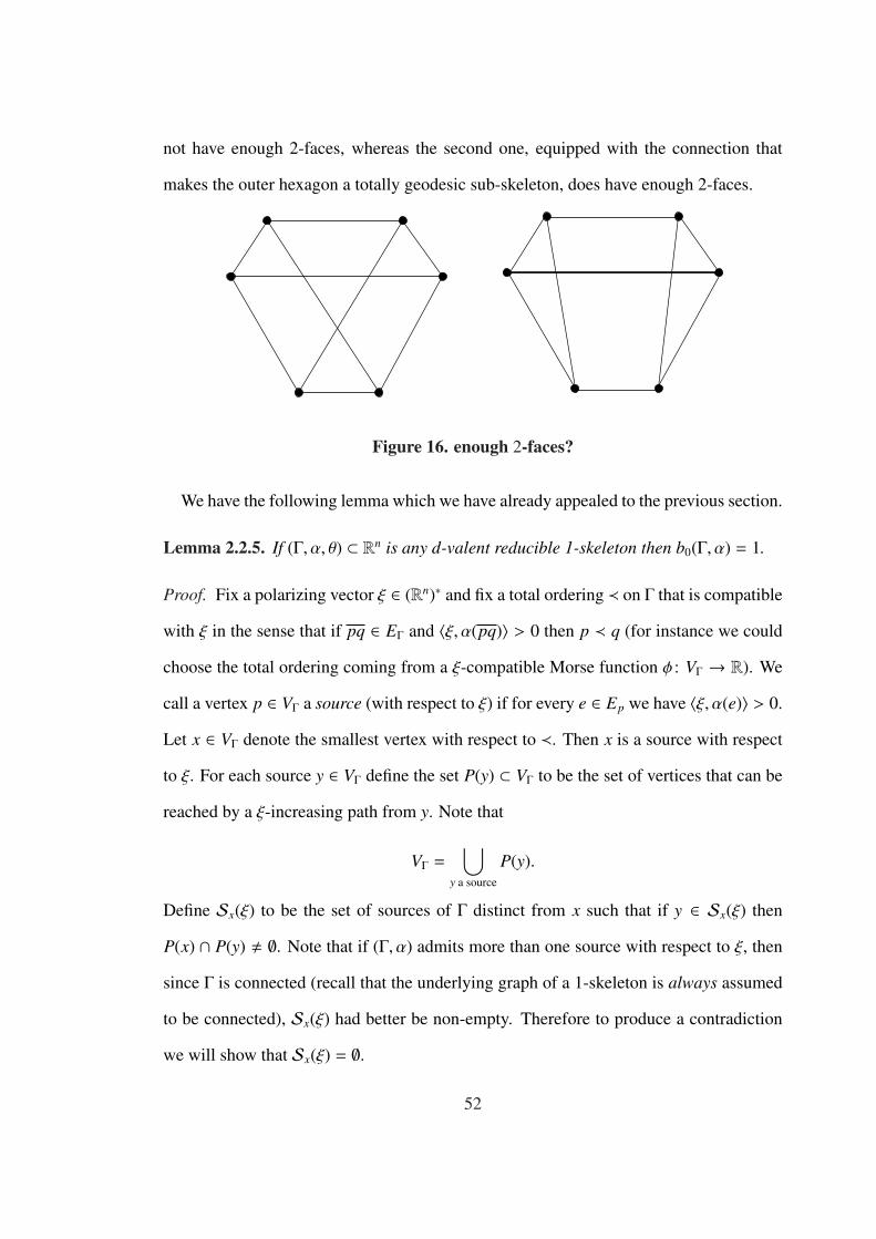
not have enough 2-faces, whereas the second one, equipped with the connection that

makes the outer hexagon a totally geodesic sub-skeleton, does have enough 2-faces.

Figure 16. enough 2-faces?

We have the following lemma which we have already appealed to the previous section.

Lemma 2.2.5. If (Γ, α, θ) ⊂ Rn is any d-valent reducible 1-skeleton then b0(Γ, α) = 1.

Proof. Fix a polarizing vector ξ ∈ (Rn)∗ and fix a total ordering ≺ on Γ that is compatible

with ξ in the sense that if pq ∈ EΓ and 〈ξ, α(pq)〉 > 0 then p ≺ q (for instance we could

choose the total ordering coming from a ξ-compatible Morse function φ : VΓ → R). We

call a vertex p ∈ VΓ a source (with respect to ξ) if for every e ∈ Ep we have 〈ξ, α(e)〉 > 0.

Let x ∈ VΓ denote the smallest vertex with respect to ≺. Then x is a source with respect

to ξ. For each source y ∈ VΓ define the set P(y) ⊂ VΓ to be the set of vertices that can be

reached by a ξ-increasing path from y. Note that

VΓ =⋃

y a source

P(y).

Define Sx(ξ) to be the set of sources of Γ distinct from x such that if y ∈ Sx(ξ) then

P(x) ∩ P(y) , ∅. Note that if (Γ, α) admits more than one source with respect to ξ, then

since Γ is connected (recall that the underlying graph of a 1-skeleton is always assumed

to be connected), Sx(ξ) had better be non-empty. Therefore to produce a contradiction

we will show that Sx(ξ) = ∅.

52

Assume that Sx(ξ) , ∅. Define the function f : Sx(ξ) → VΓ by f (y) = z where z is

the smallest vertex (with respect to ≺) in P(x) ∩ P(y). f must achieve a minimum at

some y0 ∈ Sx(ξ); set f (y0) = z0. There exist vertices v ∈ P(x) and w ∈ P(y0) such that

z0v, z0w ∈ Ez are oriented into z0 with respect to ξ (i.e. v,w ≺ z0). By the minimality of

z0 we must have v , w. Let Q be the unique 2-face spanned by the edges z0v, z0w and let

sQ ∈ VQ be the unique source of Q with respect to the polarization induced on Q by ξ.

Then there is some source y′ ∈ VΓ such that sQ ∈ P(y′). There are two cases to consider:

1. y′ = x in which case f (y0) � w ≺ z0, contradicting the minimality of z0.

2. y′ , x in which case y′ ∈ Sx(ξ) and f (y′) � v ≺ z0, again contradicting the minimality

of z0.

Hence we conclude that Sx(ξ) must have been empty in the first place and this concludes

the proof of Lemma 2.2.5. �

Before introducing the reduction operation, we must introduce one more preliminary

notion.

2.2.2 Pre-1-Skeleta and Generalized 1-Skeleta

In order to use reduction to solve the problem at hand we must loosen the genericity

requirements on the projection maps. In the next section we will see that the reduction

operation takes a d-valent k-independent 1-skeleton with connection in Rn (for k ≥ 3),

and produces a (d − 1)-valent (k − 1)-independent 1-skeleton with connection in Rn−1.

If k = 2 then reduction still produces something resembling a 1-skeleton with a graph,

connection, and even compatiblity constants, but the assignment of directions to the

edges may fail to satisfy A1 of Definition 1.1.2. In this case reduction will produce a

generalized 1-skeleton.

Let (Γ, θ) be a d-valent graph-connection pair.

53

Definition 2.2.6. A compatibility system for the pair (Γ, θ)

λ B {λe}e∈EΓ

is a collection of maps λe : Ei(e) → R+ indexed by the oriented edges of Γ that satisfy the

following rule:

λe ◦ θe =1λe

for every pair e, e ∈ EΓ.

Definition 2.2.7. A pre-1-skeleton is a triple consisting of a d-valent graph Γ, a connec-

tion θ on Γ and a compatibility system for the pair (Γ, θ). We denote this by (Γ, θ, λ).

Definition 2.2.8. A generalized axial function α compatible with the pre-1-skeleton

(Γ, θ, λ) is a map α : EΓ → Rn that satisfies the following axioms:

gA1. For each e ∈ EΓ there is some me > 0 such that α(e) = −meα(e)

gA2. For every e ∈ EΓ and each e′ ∈ Ei(e) \ {e} we have

α(e′) − λe(e′)α(θe(e′)) = ce(e′) · α(e)

for some ce(e′) ∈ R.

Definition 2.2.9. A d-valent generalized 1-skeleton in Rn is a quadruple consisting of the

data triple of a d-valent pre-1-skeleton (Γ, θ, λ) together with a generalized axial function

α : EΓ → Rn compatible with the pre-1-skeleton. We denote this by (Γ, α, θ, λ) ⊂ Rn.

Definition 2.2.10. Two generalized 1 skeleta (Γ, α, θ, λ) ⊂ Rn and (Γ, α, θ, λ) ⊂ Rn are

equivalent if

i. (Γ, θ) = (Γ, θ)

54

ii. there exists a function κ : EΓ → R+ such that for every e ∈ EΓ, we have

λe(e′) =κ(e′)

κ(θe(e′))λe(e′),

for each e′ ∈ Ei(e) \ {e}

iii. the following diagram commutes:

Rn Rnidoo

EΓ π//

Cα

OO

EΓ

α

OO.

We will denote equivalence of generalized 1-skeleta by

(Γ, α, θ, λ) ≡ (Γ, α, θ, λ)

Notice that a 1-skeleton with connection together with its compatiblity constants is

also a generalized 1-skeleton.

2.2.3 Reduction and Cross-Sections

In this construction, we start with the data of a (reducible) 1-skeleton, but the resulting

data will be that of a generalized 1-skeleton.

Let (Γ, α, θ) ⊂ Rn be a reducible (as in Definition 2.2.4) d-valent 1-skeleton with

connection with compatiblity constants λ = {λe}e∈EΓ. Fix a polarizing vector ξ ∈ (Rn)∗

and a ξ-compatible Morse function φ : VΓ → R.

Let (Γ0, α0, θ0) ⊂ (Γ, α, θ) be a 2-face. We can label the vertices V0 = {p0, . . . , pN}such that pi pi+1 ∈ E0 for 0 ≤ i ≤ N. Hence we can represent (Γ0, α0, θ0) as a loop in

Γ, p0 � · · · � p0, and we can do this in two ways (up to cyclic permutation of the

indicies): Q B {p0 � p1 � · · · � pN � p0} and Q B {p0 � pN � · · · � p1 � p0}.

55

Each representation of (Γ0, α0, θ0) is called an oriented 2-face, denoted by Q or Q for

notational convenience.

Let F2 denote the set of oriented 2-faces of (Γ, α, θ). For Q ∈ F2 let

Mξ(Q) = maxv∈Q

(φ(v))

and

mξ(Q) = minv∈Q

(φ(v)).

Fix c ∈ R a φ-regular value. Define the new graph Γc = (Vc, Ec) whose vertex set is

defined to be the oriented edges at c-level:

Vc = {pq ∈ EΓ | φ(p) < c < φ(q)}.

Consider a 2-face Q ∈ F2 at c-level, meaning that mξ(Q) < c < Mξ(Q). Let b and t

be vertices of Q such that φ(b) = mξ(Q) and φ(t) = Mξ(Q). Then since Q is a 2-face

we have b0(Q) = 1 hence there are exactly two ξ-oriented paths from b to t, γ` and

γr. For each such path, there is exactly one directed edge that crosses the c-level; i.e.

there exist unique directed edges pq, vw ∈ Vc such that γ` : b � · · · p � q · · · � t and

γr : b � · · · v � w · · · � t. Moreover only one of the oriented edges pq, vw is oriented

with respect to Q; i.e. Q = {b � · · · � p � q � · · · � w � v � · · · � b} and

Q = {b � · · · � v � w � · · · � q � p � · · · � b}. In this way an oriented 2-face Q ∈ F2

at the c-level gives an ordered pair of “vertices” in Vc; we write i(Q) = pq and t(Q) = vw.

Therefore we define the oriented edge set of Γc to be the set of oriented 2-faces at c-level:

Ec = {Q ∈ F2 | mξ(Q) < c < Mξ(Q)}.

For every pq ∈ Vc the oriented 2-faces containing pq are in one-to-one correspondence

with the oriented edges Ep\{pq}. Indeed since (Γ, α, θ) has enough 2-faces (this is part of

being reducible), any two oriented edges at p span an oriented 2-face, hence any oriented

56

edge in Ep \ {pq} together with pq define an oriented 2-face Q with i(Q) = pq. Thus Γc

is a (d − 1)-valent graph ((d − 1) is the number of oriented edges in the set |Ep \ {pq}|).There are two natural connections on Γc. Fix Q ∈ Ec and let i(Q) = pq and t(Q) = vw.

Let

γuQ : q = r1 � r2 � . . . � rk−1 � rk = w

be the upper path in Q from q to w, meaning that φ(ri) > c for 1 ≤ i ≤ k. Let

γdQ : p = t1 � t2 � . . . � tm−1 � tm = v

be the lower path in Q from p to v, meaning that φ(t j) < c for 1 ≤ j ≤ m.

The set (Ec)pq \ {Q} is in one-to-one correspondence with the oriented edges normal to

Q at p (or q), N0p (� N0

q ). Similarly the set (Ec)vw \ {Q} is in one-to-one correspondence

with the oriented edges normal to Q at v (or w), N0v (� N0

w). The normal path-connection

maps on Γ,

K⊥γuQ

: N0q → N0

w

and

K⊥γd

Q: N0

p → N0v ,

define connection maps on Γc: The up connection map along Q ∈ Ec, (θuc)Q, is defined to

be the unique map which makes the following diagram commute:

(Ec)pq \ {Q} (θuc )Q

//

�²²

(Ec)vw \ {Q}�

²²

N0q K⊥

γuQ

// N0w.

57

The down connection map along Q ∈ Ec, (θdc )Q, is defined analogously by

(Ec)pq \ {Q} (θdc )Q

//

�²²

(Ec)vw \ {Q}�

²²

N0p K⊥

γdQ

// N0v .

We have attempted to illustrate the situation in Figure 17. The bold line segments joining

the open dots represent the oriented edges issuing from the vertices pq and vw in Vc. The

line segments issuing from vertices of Q but not lying in Q itself represent those edges

normal to Q.

s1

s2sm−1

sm

u 1

u 2u k−1

u k

t 2t m−1

v=t m

kw=r

rk−1

r2

γuQ

γdQ

r=q1

p=t 1

ξ Γc

....

....

QWξ

Figure 17. the c-cross-section

We define compatibility constants for the graph-connection pairs (Γc, θuc) and (Γc, θ

dc )

58

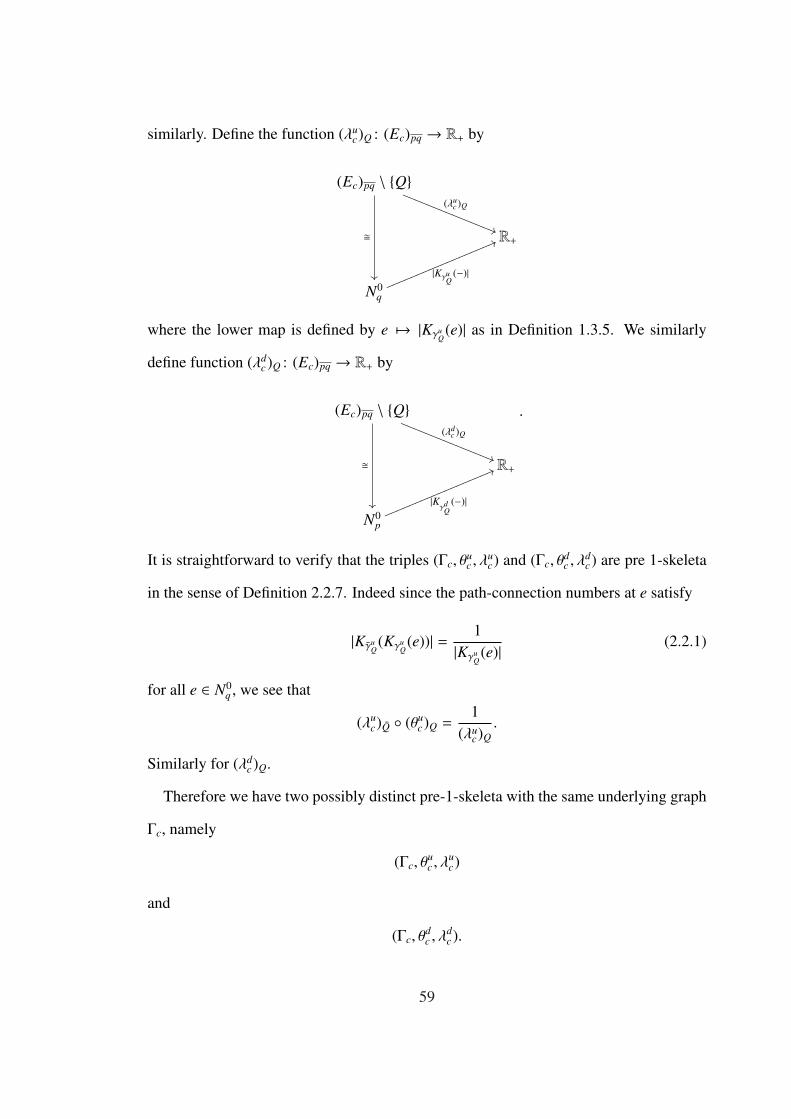
similarly. Define the function (λuc)Q : (Ec)pq → R+ by

(Ec)pq \ {Q}

�

²²

(λuc )Q

))RRRRRRRRRRRRRRR

R+

N0q

|KγuQ

(−)|

66llllllllllllllllll

where the lower map is defined by e 7→ |KγuQ(e)| as in Definition 1.3.5. We similarly

define function (λdc)Q : (Ec)pq → R+ by

(Ec)pq \ {Q}

�

²²

(λdc )Q

))RRRRRRRRRRRRRRR

R+

N0p

|Kγd

Q(−)|

66llllllllllllllllll

.

It is straightforward to verify that the triples (Γc, θuc , λ

uc) and (Γc, θ

dc , λ

dc) are pre 1-skeleta

in the sense of Definition 2.2.7. Indeed since the path-connection numbers at e satisfy

|KγuQ(Kγu

Q(e))| = 1

|KγuQ(e)| (2.2.1)

for all e ∈ N0q , we see that

(λuc)Q ◦ (θu

c)Q =1

(λuc)Q

.

Similarly for (λdc)Q.

Therefore we have two possibly distinct pre-1-skeleta with the same underlying graph

Γc, namely

(Γc, θuc , λ

uc)

and

(Γc, θdc , λ

dc).

59

For each pre-1-skeleton defined above, we can define a compatible, generalized axial

function on Γc as follows. Let Wξ ⊂ Rn denote the sub-space annihilated by ξ. Denote

by∧2Rn the vector space of alternating two tensors generated by elements of the form

x ∧ y(= −y ∧ x) for x, y ∈ Rn. Let ι :∧2Rn → Rn denote the ξ-interior product map

defined by ι(x ∧ y) = 〈ξ, x〉y − 〈ξ, y〉x. As above let Q ∈ Ec be an oriented 2-face with

i(Q) = pq and t(Q) = vw. Let

γuj : q = r1 � r2 � . . . � r j

be the partial upper path in Q from q to r j and

γdj : p = t1 � t2 � . . . � t j

the partial lower path in Q from p to t j. Then γuk = γu

Q : q � · · · � rk = w and γdm =

γdQ : p � · · · � tm = v as above. Our convention will be to let p = r0 and v = rk+1 and to

let q = t0 and w = tm+1.

Define the function

αuc : Ec → Wξ

by

αuc(Q) =

ι(α(r1r0) ∧ α(r1r2))〈ξ, α(r1r0)〉 .

Similarly define

αdc : Ec → Wξ

by

αdc(Q) =

ι(α(t1t0) ∧ α(t1t2))〈ξ, α(t1t0)〉 .

Lemma 2.2.11. The functions αuc and αd

c are compatible with the pre-1-skeleta (Γc, θuc , λ

uc)

and (Γc, θdc , λ

dc), respectively.

60

Proof. We will show that αuc is compatible with the pre-1-skeleton (Γc, θ

uc , λ

uc). The proof

that αdc is compatible with (Γc, θ

dc , λ

dc) is similar. We will follow the argument presented

in [14] more or less verbatim.

For vectors a, b, c ∈ Rn we will write

a ≡ b mod c

to mean that

a − b ∈ spanR{c}.

Fix R ∈ (Ec)pq \ {Q}. We want to show that

αuc(R) − (λu

c)Q(R) · αuc((θu

c)Q(R)) ≡ 0 mod αuc(Q).

Let qu1 ∈ N0q be the oriented edge at q (= r1) corresponding to R. Let r ju j = K⊥γu

j(r1u1) ∈

N0r j

. Then we have

αuc(R) =

ι(α(r1r0) ∧ α(r1u1))〈ξ, α(r1r0)〉

and

αuc((θu

c)Q(R)) =ιξ(α(rkrk+1) ∧ α(rkuk))〈ξ, α(rkrk+1)〉 .

The reader may find it helpful to consult Figure 17 here.

For convenience we will adopt the following temporary notation. Let

v j Bα(r jr j−1)〈ξ, α(r jr j−1)〉

v′j Bα(r jr j+1)〈ξ, α(r jr j+1)〉

and

w j B α(r ju j).

We then have

αuc(Q) = ι(v1 ∧ v′1)

61

αuc(R) = ι(v1 ∧ w1)

and

αuc((θu

c)Q(R)) = ι(v′k ∧ wk).

A direct computation will verify that

ι(v′j ∧ w j) ≡ ι(v j ∧ w j) mod αuc(Q) (2.2.2)

Also we have

w j − λr jr j+1(r ju j)w j+1 ≡ 0 mod v′j

by A3 in Definition 1.1.2. Hence we get that

ι(v′j ∧ w j) = λr jr j+1(r ju j)ι(v j+1 ∧ w j+1). (2.2.3)

Combining (2.2.2) and (2.2.3) we get

ι(v j ∧ w j) ≡ λr jr j+1(r ju j)ι(v j+1 ∧ w j+1) mod αuc(Q)

hence inductively we get

ι(v1 ∧ w1) ≡ |Kγuk(r1u1)| · ι(vk ∧ wk) mod αu

c(Q). (2.2.4)

Combining (2.2.2) with (2.2.4) we get

ι(v1 ∧ w1) ≡ |Kγuk(r1u1)| · ι(v′k ∧ wk) mod αu

c(Q),

hence we see that

αuc(R) − (λu

c)Q(R)αuc(R′) ≡ 0 mod αu

c(Q).

�

Thus we get two (possibly distinct) generalized 1 skeleta structures on the (d − 1)-

valent graph Γc; we have the up c-cross-section of Γ, (Γc, αuc , θ

uc , λ

uc), and the down c-

cross-section of Γ, (Γc, αdc , θ

dc , λ

dc).

62

2.3 Product Constructions and the Blow-Up

In this section we will describe some basic constructions that allow us to “build” new

1-skeleta from old. These constructions are crucial to what follows in this chapter, and

they will come up again in chapter 4.

2.3.1 Direct Product

Let (Γ′, α′, θ′) ⊂ Rn and (Γ0, α0, θ0) ⊂ Rm be 1-skeleta with connections. We define a

new 1-skeleton with connection (Γ, α, θ) ⊂ Rn × Rm as follows. Set

VΓ B VΓ′ × VΓ0 ,

and

EΓ B EΓ′ × VΓ0 t VΓ′ × EΓ0 .

Then Γ = (VΓ, EΓ) is just the product graph. There is a natural connection θ on Γ defined

by

θe(e) =

θ′e′(e′) × v0 if e = e′ × v0 and e = e′ × v0

t(e′) × e0 if e = e′ × v0 and e = i(e′) × e0

v′ × (θ0)e0(e0) if e = v′ × e0 and e = v′ × e0

e′ × t(e0) if e = v′ × e0 and e = e′ × i(e0)

.

θ is called the product connection on Γ.

There is a natural axial function on Γ that is compatible with θ defined by

α : EΓ → Rn × Rm

α(e) =

(α′(e′), 0) if e = e′ × v0

(0, α0(e0)) if e = v′ × e0.

63

It is straight forward to check that α is an axial function compatible with the graph-

connection pair (Γ, θ). The 1-skeleton (Γ, α, θ) ⊂ Rn × Rm is called the direct product

1-skeleton with factors (Γ′, α′, θ′) and (Γ0, α0, θ0). We can compute the compatibility

system for (Γ, α, θ) in terms of the compatibility system for the factors. We have

λe(e) =

λe′(e′) if e = e′ × {v0}, e = e′ × {v0}

λe0(e0) if e = {v′} × e0, e = {v′} × e0

1 otherwise.

The 1-skeleton in Figure 18 is a direct product whose factors are the triangle in R2 and

the single edge in R.

Figure 18. direct product

2.3.2 Tilted Product

Let (Γ′, α′, θ′) ⊂ Rn and (Γ0, α0, θ0) ⊂ Rm be given 1-skeleta with connections. As

before let (Γ, α, θ) ⊂ Rn × Rm denote the direct product 1-skeleton.

Definition 2.3.1. A tilt on (Γ, α, θ) ⊂ Rn × Rm is a map

η : VΓ′ → HomR(Rm,Rn)

with the property that for each y ∈ Rm, composition with the evaluation map

εy : HomR(Rm,Rn)→ Rn

64

εy( f ) B f (y)

gives an equivariant cohomology class on (Γ′, α′),

εy ◦ η ∈ H(Γ′, α′).

We can use a tilt on the direct product 1-skeleton to define another axial function for

the pair (Γ, θ).

Definition 2.3.2. Given a tilt η on (Γ, α, θ), define the (η-) tilted axial function

αη : EΓ → Rn × Rm

by

αη(e) =

α′(e′)

0

if e = e′ × {v0}

ηv′(α0(e0))

α0(e0)

if e = {v′} × e0

It is straight forward to check that αη is actually an axial function for the pair (Γ, θ).

Indeed, label the oriented edges of the form e′× {v0} by EhΓ

(“h” for horizontal) and those

of the form {v′} × e0 by EvΓ

(“v” for vertical).

Along a vertical edge e ∈ EvΓ

it follows by the linearity of ηv′ that

αη(e) − λe(e) · αη(θe(e)) ≡ 0 mod αη(e) (2.3.1)

for all e ∈ Ei(e).

Along a horizontal edge e ∈ EhΓ, (2.3.1) clearly holds for e ∈ Eh

Γ. On the other hand, if

e ∈ EvΓ

then we have

αη(e) =

ηv′(α0(e0))

α0(e0)

65

and

αη(θe(e)) =

ηv′′(α0(e0))

α0(e0)

where e = v′v′′ × {v0} and e = {v′} × e0. Thus (2.3.1) becomesηv′(α0(e0))

α0(e0)

−

ηv′′(α0(e0))

α0(e0)

=

ηv′(α0(e0)) − ηv′′(α0(e0))

0

.

Since the function η(α0(e0)) : VΓ′ → Rn is an equivariant class for (Γ′, α′) we conclude

that ηv′(α0(e0)) − ηv′′(α0(e0)) ≡ 0 mod α′(v′v′′). Hence αη is indeed an axial function for

the pair (Γ, θ).

Definition 2.3.3. We call (Γ, αη, θ) ⊂ Rn × Rm the (η-)tilted product 1-skeleton with

straight factor (Γ′, α′, θ′) and tilted factor (Γ0, α0, θ0).

The 1-skeleton in Figure 19 is a tilted product in R3 with straight factor the single edge

in R and tilted factor the triangle in R2. Compare this with the direct product 1-skeleton

shown in Figure 18.

Figure 19. tilted product

Note that the compatiblity system for (Γ, αη, θ) is the same as the compatibility system

for (Γ, α, θ).

66

2.3.3 Blow-Up

Fix a d-valent 1-skeleton with connection (Γ, α, θ) ⊂ Rn with compatibility constants

λ = {λe}e∈EΓand let (Γ0, α0, θ0) be a k-valent totally geodesic sub-skeleton. We will define

a new graph Γ] = (V], E]) by “replacing” Γ0 by a new (d − 1)-valent sub-graph.

Let N0 =⊔

p∈VΓ0N0

p be the set of oriented edges normal to Γ0. Define the vertex set of

Γ] to be

V] B VΓ \ V0 t N0.

We will write ze to denote a vertex corresponding to an oriented edge e ∈ N0 or we may

write zpe to denote the vertex corresponding to e ∈ N0

p.

There is a natural map of sets

β : V] → VΓ

β(x) =

q if x = q ∈ VΓ \ V0

p if x = ze for some e ∈ N0p

We declare two vertices x, y ∈ VΓ] to be adjacent if β(x) = β(y) or β(x)β(y) ∈ EΓ.

Denote this oriented edge set E]. To avoid confusion we will use the letter ε to denote

oriented edges in E]. For a vertex q ∈ VΓ \ V0 the map β furnishes a bijection between

the oriented edge sets E]q and Eβ(q). For vertices zp

e ∈ V] there is still a bijective corre-

spondence between the oriented edge sets E]

zpe

and Eβ(zpe ) given by:

E]

zpe

ψ// Ep

zpe zp

e′// e

zpe zq

f// pq

zpe [t(e)] // e

(2.3.2)

67

(in the last line t(e) denotes the terminal vertex of e in VΓ \ V0). See Figure 20. In

particular the graph Γ] is d-valent. We call Γ] the blow-up graph of Γ along Γ0. The

sub-graph Γ]0 B β−1(Γ0) ⊂ Γ] is a connected (d − 1)-valent sub-graph called the singular

locus of the blow-up.

z f’q

z ep

z e’p

p

e

e’ f’

z fq

q

f

Γ#0

Γ0

Figure 20. blow-up along a sub-skeleton

We want to define a connection and compatibility system on Γ]. The map β : V] → VΓ

extends, by its very definition, to a morphism of graphs β : Γ] → Γ. For each vertex

x ∈ V] denote by (E]x)h B β−1(Eβ(x)), the horizontal edges at x and by (E]

x)v B E]x \ (E]

x)h

the vertical edges. For each ε ∈ E] define the map θ]ε : E]i(ε) → E]

t(ε) so that the following

diagram commutes:

E]i(ε)

θ]ε //

�²²

E]t(ε)

�²²

Eβi(ε) �// Eβ(t(ε));

(2.3.3)

here the right (resp. left) vertical map labelled � is taken to be the correpondence induced

by β if i(ε) ∈ VΓ \ V0 (resp. t(ε) ∈ VΓ \ V0) or the correspondence given by (2.3.2), if

i(ε) (resp. t(ε)) = ze for some e ∈ N0. The bottom map is then taken to be either the

68

connection map θβ(ε) if ε is horizontal, or the identity if ε is vertical.

This defines a connection θ] B {θ]ε}ε∈E] on Γ]. Moreover with this connection the

morphism of graphs β is actually a morphism of graph-connection pairs β : (Γ], θ]) →(Γ, θ); this follows immediately from (2.3.3) and Definition 1.6.1.

In order to define a compatibility system for the pair (Γ], θ]) which will support the

desired (generalized) axial function, we need to assume that the sub-skeleton (Γ0, α0, θ0)

is level. We have the following technical Lemma.

Lemma 2.3.4. If the totally geodesic sub-skeleton (Γ0, θ0, α0) is level in the sense of

Definition 1.3.6 then there exists a map

n : N0 → R+

such that for every edge e ∈ E0 and every edge at e′ ∈ N0i(e) we have

n(e′)n(θe(e′))

= λe(e′). (2.3.4)

Proof. Fix a base point p ∈ V0. Let H denote the permutation sub-group of the set

Ep consisting of holonomy maps Kγ for loops γ in Γ0 based at p. Then the set N0p is

H-invariant, hence we can partition the normal edges at p into H-orbits:

N0p =

M⊔

c=1

N0p(c).

Fix representatives ep(c) ∈ N0p(c) for 1 ≤ c ≤ M. Define n(ep(c)) B 1 for 1 ≤ c ≤ M.

Using (2.3.4) we can extend n to all of N0 as follows. Given p′ ∈ VΓ0 distinct from p, fix

e′ ∈ N0p′ . Let γ ⊂ Γ0 be any path joining p to p′ such that the path-connection map for γ

gives Kγ(ep(c)) = e′ for some 1 ≤ c ≤ M. Note that while the path γ may not be unique,

the representative ep(c) is unique. Define

n(e′) B1

|Kγ(ep(c))| .

69

The map

n : N0 → R+

is independent of the path γ since (Γ0, α0, θ0) is level; hence n is well-defined. Since

n(θe(e′)) =1

|θe ◦ Kγ(ep(c))| =1

λe(e′)· 1|Kγ(ep(c))| ,

we clearly have that n(e′)n(θe(e′)) = λe(e′) and this completes the proof of Lemma 2.3.4. �

The map in Lemma 2.3.4 is called a blow-up system for Γ along Γ0. We assume for

the rest of this section that the sub-skeleton (Γ0, α0, θ0) is level and we fix some choice

of blow-up system n : N0 → R+.

We are now in a position to define λ]. Fix ε ∈ E]. There are two cases to consider

here.

For ε ∈ (E])v define

(E]i(ε))

v λ]ε // R+

zeze′// n(e)

n(e′′)

(2.3.5)

where ε = zeze′′ , and

(E]i(ε))

h λ]ε // R+

ε′ // 1.

(2.3.6)

For ε ∈ (E])h: On vertical edges ε′ = zeze′ ∈ (E]i(ε))

v define

λ]ε(ε′) = λβ(ε)(e) · λβ(ε)(e′). (2.3.7)

On horizontal edges define λ]ε : (E]i(ε))

h → R+ so that the following diagram commutes:

(E]i(ε))

h λ]ε //

β

²²

R+

Eβ(i(ε))

λβ(ε)

77oooooooooooooo.

(2.3.8)

70

Let us check that λ] = {λ]ε}ε∈E] defines a compatibility system on the graph connection

pair (Γ], θ]). We must check that

λ]ε ◦ θ]ε =1

λ]ε(2.3.9)

holds for all ε ∈ E].

Along vertical edges ε ∈ (E])v:

• For each ε′ ∈ (E]i(ε))

h we have that θ]ε(ε′) ∈ (E]t(ε))

h, hence both sides of (2.3.9) evaluate

to 1 on ε′ by (2.3.6).

• For ε′ ∈ (E]i(ε))

v, let ε = zeze′ and ε′ = zeze′′ . Then θ]ε(zeze′′) = ze′ze′′ by (2.3.3). Thus by

(2.3.5), the LHS of (2.3.9) is λ]ε(zpe′z

pe′′) =

n(e′)n(e) which is exactly the reciprocal of λ]ε(z

pe zp

e′′).

This shows that (2.3.9) holds for vertical ε.

Along horizontal edges ε ∈ (E])h:

• For horizontal edges we have the following diagram:

(E]i(ε))

h θ]ε //

β

²²

(E]t(ε))

h

β

²²

λ]ε // R+

Eβ(i(ε))θβ(ε)

// Eβ(t(ε)).

λβ(ε)

77oooooooooooooo

(2.3.10)

This diagram is clearly commutative by (2.3.3) and (2.3.8). Thus it then follows that

(2.3.9) holds along ε for horizontal edges, since the analogous identity holds for θ and λ

along β(ε).

• For vertical edges ε′ = zeze′ ∈ (E]i(ε))

v let z f z f ′ ∈ (E]i(ε))

v denote the oriented edge θ]ε(ε′).

Then we have

λ]ε(θ]ε(ε′)) = λβ(ε)( f ) · λβ(ε)( f ′)

=1

λβ(ε)(e) · λβ(ε)(e′)=

1

λ]ε(ε′).

Thus (2.3.9) holds along ε for vertical edges as well.

We have defined a pre 1-skeleton (Γ], θ], λ]) called the blow-up pre 1-skeleton of

(Γ, θ, λ). The following lemma shows that a generalized 1-skeleton structure on one

71

determines a generalized 1-skeleton structure on the other (almost).

Lemma 2.3.5. Given a generalized axial function α for the pre 1-skeleton (Γ, θ, λ), there

is a generalized axial function α] for the pre 1-skeleton (Γ], θ], λ]). Conversely, given a

generalized axial function α for the pre 1-skeleton (Γ], θ], λ]) such that for all e ∈ E0 and

any two oriented edges ε, ε′ ∈ β−1(e), α(ε) = α(ε′), there is a generalized axial function

α for (Γ, θ, λ).

Proof. Let α : EΓ → Rn be a generalized axial function on (Γ, θ, λ). Define the function

α](ε) =

α(β(ε)) if ε) ∈ (E])h

n(e)α(e′) − n(e′)α(e) if ε = zeze′ ∈ (E])v.

(2.3.11)

The function α] clearly satisfies gA1 in 2.2.8. We need only show that α] satisfies

gA2.

Along vertical edges ε ∈ (E])v:

• For ε′ ∈ (E]i(ε))

h note that λ]ε(ε′) = 1. Also we have β(θ]ε(ε′)) = β(ε′) by (2.3.3). Hence

α](ε′) = α(β(ε)) = α](θ]ε(ε′)).

• For ε′ = zeze′ ∈ (E]i(ε))

v, we have λ]ε(ε′) =n(e)

n(e′′) where ε = zeze′′ . Furthermore we have

θ]ε(ε′) = ze′′ze′ and

α](ε) = n(e)α(e′′) − n(e′′)α(e),

α](ε′) = n(e)α(e′) − n(e′)α(e)

and

α](θ]ε(ε′)) = n(e′′)α(e′) − n(e′)α(e′′).

Hence in this case we have α](ε′) − λ]ε(ε′)α](θ]ε(ε′)) =n(e′)n(e′′)α

](ε).

Along horizontal edges ε ∈ (E])h:

• For ε′ ∈ (E]i(ε))

h, we have λ]ε(ε′) = λβ(ε)(β(ε′)), β(θ]ε(ε′)) = β(θβ(ε)(β(ε′))) and α](ε′) =

72

α(β(ε′)) on (E])h. Hence we have

α](ε′) − λ]ε(ε′)α](θ]ε(ε′)) = α(β(ε′)) − λβ(ε)(ε′)α(θβ(ε)(β(ε′)))

= c · α(β(ε)) = c · α](ε)

for some c ∈ R.

• For ε′ = zeze′ ∈ (E]i(ε))

v we have θ]ε(ε′) = z f z f ′ where f = θβ(ε)(e) and f ′ = θβ(ε)(e′). Also

λ]ε(ε′) = λβ(ε)(e) · λβ(ε)(e′) by (2.3.7). We have

α](ε) = α(β(ε)),

α](ε′) = n(e)α(e′) − n(e′)α(e),

and

α](θ]ε(ε′)) = n( f )α( f ′) − n( f ′)α( f ).

Here is where we use condition 2.3.4 in Lemma 2.3.4. The point is that n(e)n( f ) = λβ(ε)(e)

and n(e′)n( f ′) = λβ(ε)(e′). Hence we have

α](ε′) − λ]ε(ε′)α](θ]ε(ε′)) =

n(e)α(e′) − n(e′)α(e) − λβ(ε)(e) · λβ(ε)(e′)(n( f )α( f ′) − n( f ′)α( f )

)=

n(e)α(e′) − n(e′)α(e) − n(e)n( f )

n(e′)n( f ′)

(n( f )α( f ′) − n( f ′)α( f )

)=

n(e)(α(e′) − λβ(ε)(e′)α( f ′)

)− n(e′)

(α(e) − λβ(ε)(e)α( f )

)= cα(β(ε)) = cα](ε)

for some c ∈ R.

This shows that α] is a generalized axial function for the pre 1-skeleton (Γ], θ], λ]).

Now assume that α : E] → Rn is a generalized axial function for the pre 1-skeleton

(Γ], θ], λ]) with the property that for every e ∈ E0 and every pair ε, ε′ ∈ β−1(e), α(ε) =

α(ε′). Then define the function α : EΓ → Rn

α(e) = α(ε) (2.3.12)

73

where ε ∈ β−1(e). Note that the fiber β−1(e) consists only of horizontal edges of the blow-

up. Moreover β−1(e) consists of a single edge unless e ∈ E0. Hence α is well defined

(we are assuming α is constant on the non-trivial fibers β−1(e)). We verify that α is a

generalized axial function on the pre 1-skeleton (Γ, θ, λ).

By (2.3.8) we have that λ]ε(ε′) = λβ(ε)(β(ε′)) for all ε, ε′ ∈ (E]x)h, x ∈ V]. Fix e ∈ EΓ

and ε ∈ β−1(e). The important point is that β : (E]i(ε))

h → Eβ(i(ε)) is a bijection and by

(2.3.3) we have that θe(e′) = θ]ε(ε′) where ε′ ∈ (E]i(ε))

h is the unique oriented edge such

that β(ε′) = e′. It then follows that

α(e′) − λe(e′)α(θe(e′)) = α(ε′) − λ]εα(θ]ε(ε′)) = c · α(ε) = c · α(e).

This shows that α is a generalized axial function for (Γ, θ, λ), and hence completes the

proof of Lemma 2.3.5. �

Definition 2.3.6. (Γ], α], θ], λ]) is called the blow-up of Γ along Γ0.

If α] is 2-independent, then (Γ], α], θ], λ]) is a 1-skeleton with connection in the sense

of Definition 1.1.3, with compatibility system λ].

If we set βL : Rn → Rn to be the identity map on Rn and set βG B β then we get a

morphism of 1-skeleta with connection which we denote by the symbol β again

β = (βG, βL) : (Γ], α], θ])→ (Γ, α, θ).

It turns out that the morphism of 1-skeleta with connection

β0 : (Γ]0, α]0, θ

]0)→ (Γ0, α0, θ0)

is actually a fiber bundle of 1-skeleta with connection.

Remark. Guillemin and Zara introduced this beautiful construction and used it to great

effect in their paper [14]. Their set of assumptions however are a bit more restrictive

than those we make here. In particular they assume that

74

1. α is 3-independent and

2. the compatibility constants along edges of Γ0 for the normal edges are all equal to 1;

i.e. λe(e′) = 1 for e ∈ E0 and e′ ∈ N0i(e).

Note that if 2. holds then (Γ0, α0, θ0) is level and if 1. holds, the function α] is indeed an

axial function for the pair (Γ], θ]).

2.4 The Main Result

Definition 2.4.1. We say that the d-valent generalized 1-skeleton (Γ, α, θ, λ) ⊂ Rn admits

a lift if there exists a generalized axial function A : EΓ → Rd for the pre 1-skeleton

(Γ, θ, λ) that satisfies the following conditions

L1.{A(e) | e ∈ Ep

}is a basis for Rd for each p ∈ VΓ

L2. there is a surjective linear map p : Rd → Rn such that α = p ◦ A.

We call the generalized 1-skeleton (Γ, A, θ, λ) ⊂ Rd a lift of (Γ, α, θ, λ) ⊂ Rn.

We now come to the main result of this chapter. Let (Γ, α, θ, λ) ⊂ Rn be a d-valent

1-skeleton.

Theorem 2.4.2. The following are equivalent:

i. (Γ, α, θ, λ) has a non-cyclic lift

ii. (Γ, α, θ, λ) is reducible and for every regular value c ∈ R, we have (Γc, αuc , θ

uc , λ

uc) ≡

(Γc, αdc , θ

dc , λ

dc).

iii. (Γ, α, θ, λ) is reducible and every 2 face is level and has trivial normal holonomy.

75

The argument used to prove Theorem 2.4.2 runs as follows. First we prove the equiv-

alence of (ii) and (iii) which is relatively straightforward. That (i) implies (ii) is also

straightforward. The direction that requires the most work is showing that (ii) implies

(i). To this end we first show that (ii) implies that every c-cross-section has a lift. Next

we show that if (Γ, α, θ, λ) ⊂ Rn satisfies (ii), then so does the direct product (or the tilted

product) of (Γ, α, θ, λ) with an interval (we will find the characterization in (iii) useful

here). We then show that (Γ, α, θ, λ) is equivalent to a cross-section of this tilted product

1-skeleton which satisfies (ii), hence has a lift. That the lift is non-cyclic will follow from

the reducibility condition on (Γ, α, θ, λ). The remainder of this section will be devoted to

the proof of Theorem 2.4.2.

2.4.1 The Easy Part

Fix a d-valent reducible 1-skeleton (Γ, α, θ, λ) ⊂ Rn, a polarizing covector ξ ∈ (Rn)∗

and a ξ-compatible Morse function φ : VΓ → R. Fix a φ-regular value c ∈ R, and let

Q ∈ Ec be as before with i(Q) = pq, t(Q) = vw, γuQ : q = r1 � r2 � · · · � rk = w and

γdQ : p � t1 � · · · � tm = v. First we need a lemma.

Lemma 2.4.3. Let κ : Ec → R+ be the function defined by κ(Q) B λqp(qr2). Then

αuc = κ · αd

c .

Proof. First observe that the subspaces Wξ and 〈α(pq)〉 are situated transversely in Rn.

We have that

αdc(Q) = α(pt2) − 〈ξ, α(pt2)〉

〈ξ, α(pq)〉α(pq) ∈ Wξ

and

αuc(Q) = α(qr2) − 〈ξ, α(qr2)〉

〈ξ, α(qp)〉 α(qp) ∈ Wξ.

Since α(qr2) − λqp(qr2)α(pt2) ∈ 〈α(qp)〉, we have that

αuc(Q) − κ(Q)αd

c(Q) ∈ Wξ ∩ 〈ξ, α(pq)〉.

76

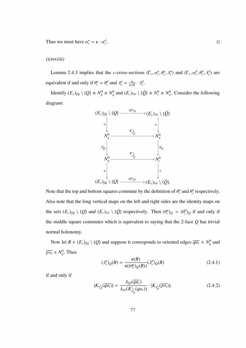
Thus we must have αuc = κ · αd

c . �

(ii)⇔(iii)

Lemma 2.4.3 implies that the c-cross-sections (Γc, αuc , θ

uc , λ

uc) and (Γc, α

dc , θ

dc , λ

dc) are

equivalent if and only if θuc = θd

c and λuc = κ

κ◦θuc· λd

c .

Identify (Ec)pq \ {Q} � N0p � N0

q and (Ec)vw \ {Q} � N0v � N0

w. Consider the following

diagram:

(Ec)pq \ {Q} (θuc )Q

//

�

²²

(Ec)vw \ {Q}

�

²²

N0q

K⊥γu

Q//

θ⊥qp

²²

N0w

θ⊥vw

²²

N0p

K⊥γd

Q//

�

²²

N0v

�

²²

(Ec)pq \ {Q} (θdc )Q

// (Ec)vw \ {Q}.Note that the top and bottom squares commute by the definition of θu

c and θdc respectively.

Also note that the long vertical maps on the left and right sides are the identity maps on

the sets (Ec)pq \ {Q} and (Ec)vw \ {Q} respectively. Then (θuc)Q = (θd

c )Q if and only if

the middle square commutes which is equivalent to saying that the 2-face Q has trivial

normal holonomy.

Now let R ∈ (Ec)pq \ {Q} and suppose it corresponds to oriented edges qu1 ∈ N0q and

ps1 ∈ N0p. Then

(λuc)Q(R) =

κ(R)κ((θu

c)Q(R))(λd

c)Q(R) (2.4.1)

if and only if

|KγuQ(qu1)| = λqp(qu1)

λwv(K⊥γuQ(qu1))

· |KγdQ(ps1)|. (2.4.2)

77

Note that λwv(K⊥γuQ(qu1)) · |Kγu

Q(qu1)| = |Kγ1(qu1)|, where γ1 : q � r2 � · · · � w � v. Also

note that λqp(qu1) · |KγdQ(ps1)| = |Kγ2(qu1)|, where γ2 : q � p � t2 � · · · � v. Therefore

(2.4.2) holds for every qu1 ∈ N0q if and only if |Kγ1(qu1)| = |Kγ2(qu1)| for every qu1 ∈ N0

q .

But this holds if and only if the 2-face Q is level.

This shows that (ii) and (iii) are equivalent.

(i)⇒ (ii)

Let (Γ, A, θ, λ) ⊂ Rd be a lift of (Γ, α, θ, λ) ⊂ Rn with respect to a projection map

p : Rd → Rn. Let p∗ : (Rn)∗ → (Rd)∗ be the dual of p. Then the covector ξ B p∗(ξ) is

a polarizing covector for (Γ, A, θ, λ). Indeed we have for every e ∈ EΓ, 〈p∗(ξ), A(e)〉 =

〈ξ, p ◦ A(e)〉 = 〈ξ, α(e)〉. Thus φ is also a ξ-compatible Morse function for (Γ, A, θ, λ).

Let c ∈ R be any φ-regular value. Then since A is d-independent, it follows that Auc

and Adc are (d − 1)-independent. By Lemma 2.4.3, we have Au

c = κ · Adc , hence we must

also have αuc = κ · αd

c . By the independence conditions on Auc , Ad

c (all we need is 2-

independence here) we are forced to have θuc = θd

c and λuc = κ

κ◦θuc· λd

c . Hence we have

(Γc, Auc , θ

uc , λ

uc) ≡ (Γc, Ad

c , θdc , λ

dc) and therefore also have (Γc, α

uc , θ

uc , λ

uc) ≡ (Γc, α

dc , θ

dc , λ

dc).

This shows that (i) implies (ii).

2.4.2 Lifting Cross-Sections

Let (Γ, α, θ, λ) be a d-valent generalized 1-skeleton with connection, (Γ0, α0, θ0, λ0) a

k-valent totally geodesic, level sub-skeleton and let n : N0 → R+ be a compatible blow-

up system. Let (Γ], α], θ], λ]) denote the corresponding blow-up generalized 1-skeleton

with connection. The following lemma is a cornerstone in the proof of Theorem 2.4.2.

Lemma 2.4.4. If (Γ, A, θ, λ) ⊂ Rd is a lift of (Γ, α, θ, λ) ⊂ Rn, then (Γ], A], θ], λ]) ⊂ Rd

is a lift of (Γ], α], θ], λ]) ⊂ Rn. Conversely if (Γ], A, θ], λ]) is a lift of (Γ], α], θ], λ]), then

78

A = A] where (Γ, A, θ, λ) is a lift of (Γ, α, θ, λ).

Proof. Let (Γ, A, θ, λ) ⊂ Rd be a lift of (Γ, α, θ, λ) ⊂ Rn via a projection map p : Rd → Rn.

Then by Lemma 2.3.5 there is a generalized axial function A] for the pre 1-skeleton

(Γ], θ], λ]) defined by (4.3.2). The axial function α] is also defined according to (4.3.2),

hence we must have p ◦ A] = α]. Since A is d-independent and {A](ε) | ε ∈ E]x} =

{A(β(ε)) | β(ε) ∈ Eβ(x)} for all x ∈ VΓ \ VΓ0 , A] must also be d-independent. Therefore

(Γ], A], θ], λ]) must be a lift of (Γ], α], θ], λ]).

Conversely suppose that (Γ], A, θ], λ]) is a lift of (Γ], α], θ], λ]) via the projection map

p : Rd → Rn. First we check that A(ε) = A(ε′) for all ε, ε′ ∈ β−1(e), e ∈ E0. Since

the fibers of β are connected, it suffices to check this in the case where i(ε) and i(ε′) are

joined by an oriented edge ε′′ ∈ (E])v. In this case we have

A(ε) − λ]ε′′(ε)A(ε′) = cA(ε′′) (2.4.3)

for some c ∈ R. The claim is that c = 0. To see this, apply the projection p to both sides

of (2.4.3) to get

α](ε) − λ]ε′′(ε)α](ε′) = cα](ε′′); (2.4.4)

On the other hand, recall that λ]ε′′(ε) = 1 and α](ε) = α](ε′). Thus the LHS of (2.4.4)

must be zero, which implies that c must also be zero.

Thus we can apply Lemma 2.3.5 to get a generalized axial function A on (Γ, θ, λ)

defined by (2.3.12). Clearly p ◦ A = α, using p ◦ A = α] and (2.3.12). Finally that A

is d-independent follows from (2.3.12) and from the fact that A] is d-independent. This

completes the proof of Lemma 2.4.4. �

In [14] Guillemin and Zara explicitly describe the changes in the cross-section in

passing over a critical value in the 3-independent non-cyclic case. Essentially they show

that two consecutive cross-sections can be blown-up to equivalent 1-skeleta. With a

79

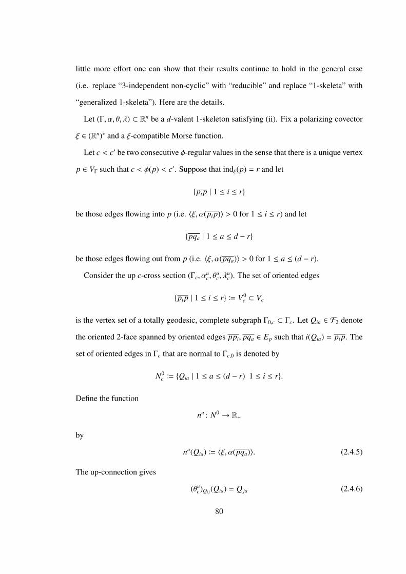
little more effort one can show that their results continue to hold in the general case

(i.e. replace “3-independent non-cyclic” with “reducible” and replace “1-skeleta” with

“generalized 1-skeleta”). Here are the details.

Let (Γ, α, θ, λ) ⊂ Rn be a d-valent 1-skeleton satisfying (ii). Fix a polarizing covector

ξ ∈ (Rn)∗ and a ξ-compatible Morse function.

Let c < c′ be two consecutive φ-regular values in the sense that there is a unique vertex

p ∈ VΓ such that c < φ(p) < c′. Suppose that indξ(p) = r and let

{pi p | 1 ≤ i ≤ r}

be those edges flowing into p (i.e. 〈ξ, α(pi p)〉 > 0 for 1 ≤ i ≤ r) and let

{pqa | 1 ≤ a ≤ d − r}

be those edges flowing out from p (i.e. 〈ξ, α(pqa)〉 > 0 for 1 ≤ a ≤ (d − r).

Consider the up c-cross section (Γc, αuc , θ

uc , λ

uc). The set of oriented edges

{pi p | 1 ≤ i ≤ r} B V0c ⊂ Vc

is the vertex set of a totally geodesic, complete subgraph Γ0,c ⊂ Γc. Let Qia ∈ F2 denote

the oriented 2-face spanned by oriented edges ppi, pqa ∈ Ep such that i(Qia) = pi p. The

set of oriented edges in Γc that are normal to Γc,0 is denoted by

N0c B {Qia | 1 ≤ a ≤ (d − r) 1 ≤ i ≤ r}.

Define the function

nu : N0 → R+

by

nu(Qia) B 〈ξ, α(pqa)〉. (2.4.5)

The up-connection gives

(θuc)Qi j(Qia) = Q ja (2.4.6)

80

and up-compatibility system gives

(λuc)Qi j(Qia) = 1 (2.4.7)

for all i, j, a. In particular we see that nu defines a blow-up system for Γc along Γ0,c.

Denote the corresponding blow-up generalized 1-skeleton by

(Γ]c, (αuc)], (θu

c)], (λuc)]).

Next consider the down c′-cross section (Γc′ , αdc′ , θ

dc′ , λ

dc′). The set of oriented edges

{pqa | 1 ≤ a ≤ d − r} B V0c′ ⊂ Vc′

is the vertex set of a totally geodesic, complete subgraph Γ0,c′ ⊂ Γc′ . Let Qai ∈ F2 denote

the oriented 2-face spanned by oriented edges ppi, pqa ∈ Ep such that i(Qai) = pqa. The

set of oriented edges in Γc′ that are normal to Γc′,0 is denoted by

N0c′ B {Qai | 1 ≤ i ≤ r 1 ≤ a ≤ (d − r)}.

Define the function

nd : N0 → R+

by

nd(Qai) B 〈ξ, α(ppi)〉. (2.4.8)

The down-connection gives

(θdc′)Qab(Qai) = Qbi (2.4.9)

and the down-compatibility system gives

(λdc′)Qab(Qai) = 1 (2.4.10)

for all a, b, i. In particular nd defines a blow-up system for Γc′ along Γ0,c′ . Denote the

corresponding blow-up generalized 1-skeleton by

(Γ]c′ , (αdc′)

], (θdc′)

], (λdc′)

]).

81

We have attempted to illustrate the situation in Figure 21.

The following lemma is an analogue of Theorem 2.3.2 in [14].

Lemma 2.4.5. (Γ]c, (αuc)], (θu

c)], (λuc)]) ≡ (Γ]c′ , (α

dc′)

], (θdc′)

], (λdc′)

])

Proof. Let βc and βc′ denote the blow-down morphisms for the up c-cross section and

the down c′-cross section, respectively. We have that

V]c = Vc \ V0

c t N0c

and

V]c′ = Vc′ \ V0

c′ t N0c′ .

The sets Vc \ V0c and Vc′ \ V0

c′ are naturally identified: if an oriented edge e ∈ EΓ does not

contain p and crosses the c-level, then it must also cross the c′-level.

The sets N0c and N0

c′ are also naturally identified by the identification

Qia ≡ Qai.

There are four types of edges in Γ]c:

1. R ∈ Ec \ {E]c,0 ∪ N0

c }

2. Qia ∈ N0c

3. QiaQib a , b (vertical in Γ]c,0)

4. QiaQ ja i , j (horizontal in Γ]c,0)

This identification V]c � V]

c′ induces an identification of graphs Γc� // Γc′ such

82

that

R �R

Qia �Qai (2.4.11)

QiaQib �QaiQbi

QiaQ ja �QaiQa j

Note that the horizontal edges in Γ]c,0 are identified with the vertical edges in Γ

]c′,0 and

vice-versa.

We would like to show that (θuc)] = (θd

c′)] under this identification of Γ

]c and Γ

]c′ . First we

check that these maps agree along oriented edges in the singular locus. Fix an oriented

edge ε ∈ (E]c,0). We can identify the oriented edges (Ec)βc(i(ε)) and (Ec′)βc′ (i(ε)) as follows.

Suppose that βc(i(ε)) = pi p and that βc′(i(ε)) = pqa. Then identify

(Ec)βc(i(ε))Ψ // (Ec′)βc′ (i(ε))

Qib // Qab

Qia // Qai

Qi j // Qa j

For notational convenience, set x = i(ε) and y = t(ε). Let

(Ec)βc(x) B (Ec)βc(x) \ {Qia}

and

(Ec′)βc′ (x) B (Ec′)βc′ (x) \ {Qai}.

83

We have the following diagram:

(E]c,0)x

(θuc )]ε

//

�

²²

ψ

((QQQQQQQQQQQQQQ (E]c,0)y

ψ

vvmmmmmmmmmmmmmm

�

²²

(Ec)βc(x)� //

Ψ

²²

(Ec)βc(y)

Ψ

²²

(Ec′)βc′ (x)� // (Ec′)βc′ (y)

(E]c′,0)x

(θdc′ )

]ε

//

ψ66mmmmmmmmmmmmmm

(E]c′,0)y

ψhhQQQQQQQQQQQQQQ

(2.4.12)

The diagonal maps are the identifications as in (2.3.2). The short horizontal maps are

taken to be either the identity if ε is vertical or θβ(ε) if ε is horizontal. The long vertical

maps are the identifications in (2.4.11) above. We want to show that the outer rectangle

commutes.

Note that the upper and lower quadrilaterals in (2.4.12) commute by definition of the

blow-up connection, as in (2.3.3). It is straightforward to check that the left and right

quadrilaterals in (2.4.12) commute:

Ψ ◦ ψ(ε) =

Ψ(Qib) if ε = QiaQib

Ψ(Qi j) if ε = QiaQ ja

=

Qab if ε = QiaQib

Qa j if ε = QiaQ ja

�ψ(ε).

Moreover one can check that the middle rectangle commutes as well. In this case note

that if ε ∈ (E]c,0)h then ε ∈ (E]

c′,0)v. By symmetry we may assume that ε = QiaQ ja ∈(E]

c,0)h. Then checking the commutativity of the middle rectangle in (2.4.12) amounts to

84

checking the commutativity of the following diagram:

(Ec)βc(x)(θu

c )β(ε)//

Ψ

²²

(Ec)βc(y)

Ψ

²²

(Ec′)βc′ (x)= // (Ec′)βc′ (y).

We compute

Ψ ◦ (θuc)β(ε)(e′) =

Ψ(Q jb) if e′ = Qib

Ψ(Q jk) if e′ = Qik

=

Qab if e′ = Qib

Qak if e′ = Qik

=Ψ(e′).

This shows that the middle rectangle in (2.4.12) commutes. Therefore the outer rect-

angle in (2.4.12) must also commute. Thus we have (θuc)] = (θd

c′)] along the singular

locus under the identification of the singular loci Γ]c,0

� // Γ]c′,0 in (2.4.11).

To see that these two connections agree outside of the singular locus, we need the 2-

faces at the c-level to have trivial normal holonomy, which holds since (Γ, α, θ, λ) satisfies

(ii) (which we showed is equivalent to (iii)).

It is straightforward to see that for oriented edges ε ∈ E]c disjoint from the singular

locus, (θuc)]ε = (θd

c′)]ε . Indeed such oriented edges correspond to oriented 2-faces R at the

c-level that do not contain the vertex p. Hence R is also at the c′ level and in this case

(θuc)]R = (θu

c)R and (θdc′)

]R = (θd

c′)R. Moreover there is a natural identification of (θdc′)R with

(θdc )R. Since R has trivial normal holonomy, it follows that (θu

c)R = (θdc )R. We leave it as

an exercise to verify that (θuc)] agrees with (θd

c′)] along the oriented edges normal to the

singular locus ε ∈ β−1c (N0

c ).

85

Hence we actually have an identification of graph connection pairs

(Γ]c, (θuc)]) � (Γ]c′ , (θ

dc′)

]).

We will now show that this extends to an equivalence of generalized 1-skeleta.

Define the function

E]c ≡ E]

c′κ // R+

R // λqp(qr)

Qia // 〈ξ,α(pqa)〉〈ξ,α(pi p)〉

QiaQib// 〈ξ, α(pqa)〉

QiaQ ja// 1〈ξ,α(pi p)〉

(2.4.13)

where R = {p � q � r � · · · }. We need to check that (αuc)] = κ · (αd

c′)] and that

(λuc)]ε = κ

κ◦(θuc )]ε· (λd

c′)]ε for all ε ∈ E]

c ≡ E]c′ as in Definition 2.2.10.

• For edges R ∈ E]c ≡ E]

c′ of type 1:

Then R is an oriented 2-face of (Γ, α, θ, λ) that does not contain the vertex p. Also we

have that αdc′(R) = αd

c(R). Thus by Lemma 2.4.3 we have

(αuc)](R) = αu

c(R) = ·αdc(R) = λqp(qr) · αd

c′(R) = λqp(qr) · (αdc′)

].

Thus

(αuc)](R) = κ(R) · (αd

c′)](R)

for R = {p � q � r � · · · } ∈ E]c \ {E]

c,0 ∪ N]c,0}.

• For edges Qia ∈ N]c,0 of type 2:

We have

(αuc)](Qia) =

ι(α(ppi) ∧ α(pqa))〈ξ, α(ppi)〉 .

86

On the other hand we have

(αdc′)

](Qai) =ι(α(pqa) ∧ α(ppi))〈ξ, α(pqa)〉 .

Therefore we have

〈ξ, α(pqa)〉〈ξ, α(pi p)〉 (α

dc′)

](Qai) =〈ξ, α(pqa)〉〈ξ, α(pi p)〉

ι(α(pqa) ∧ α(ppi))〈ξ, α(pqa)〉 =

ι(α(pqa) ∧ α(ppi))〈ξ, α(pi p)〉 =

ι(α(ppi) ∧ α(pqa))〈ξ, α(ppi)〉 = (αu

c)](Qia)

(in this penultimate equality we are appealing to the fact that α(pi p) = −α(ppi) as in A2

in Definition 1.1.2). Thus we have (αuc)](Qia) = κ(Qia) · (αd

c′)](Qai).

• For edges QiaQib of type 3:

We have

(αuc)](QiaQib) = nu(Qia)αu

c(Qib) − nu(Qib)αuc(Qia) =

〈ξ, α(pqa)〉 · ι(α(ppi) ∧ α(pqb))〈ξ, α(ppi)〉 − 〈ξ, α(pqb)〉 · ι(α(ppi) ∧ α(pqa))

〈ξ, α(ppi)〉 =

〈ξ, α(pqa)〉α(pqb) − 〈ξ, α(pqb)〉α(pqa) =

ι(α(pqa) ∧ α(pqb)) = 〈ξ, α(pqa)〉 · αdc′(Qab) = 〈ξ, α(pqa)〉 · (αd

c′)](QaiQbi).

Hence (αuc)](QiaQib) = κ(QiaQib) · (αd

c′)](QaiQbi).

• For edges QiaQ ja ∈ (E]c,0)h of type 4:

We have

(αuc)](QiaQ ja) = αu

c(Qi j) =ι(α(ppi) ∧ α(pp j))〈ξ, α(ppi)〉 .

On the other hand we have

(αdc′)

](QaiQa j) = nd(Qai)αdc′(Qa j) − nd(Qa j)αd

c′(Qai) =

〈ξ, α(pi p)〉 · ι(α(pqa) ∧ α(pp j))〈ξ, α(pqa)〉 − 〈ξ, α(p j p)〉 · ι(α(pqa) ∧ α(ppi))

〈ξ, α(pqa)〉 =

87

〈ξ, α(pi p)〉α(pp j) − 〈ξ, α(p j p)〉α(ppi) = ι(α(ppi) ∧ α(pp j)) = 〈ξ, α(ppi)〉(αuc)](QiaQ ja).

Thus we have (αuc)](QiaQ ja) = κ(QiaQ ja) · (αd

c′)](QaiQa j).

We leave it as an exercise to verify that (λuc)]ε = κ

κ◦(θuc )]ε· (λd

c′)]ε for all ε ∈ E]

c ≡ E]c′ .

Thus we have an equivalence of generalized 1-skeleta

(Γ]c, (αuc)], (θu

c)], (λuc)]) ≡ (Γ]c′ , (α

dc′)

], (θdc′)

], (λdc′)

]).

�

Let (Γ, α, θ, λ) ⊂ Rn be any d-valent reducible 1-skeleton with connection (not nec-

essarily satisfying condition (ii) of Theorem 2.4.2). For any fixed polarizing vector

ξ ∈ (Rd)∗ and any ξ-compatible Morse function φ let c be a φ-regular value such that

there is a unique vertex p ∈ VΓ with the property that φ(p) < c. We have the following

important observation.

Lemma 2.4.6. The generalized 1-skeleton (Γc, αdc , θ

dc , λ

dc) ⊂ Rn−1 always has a lift.

Proof. Label the oriented edges at p by {pqa | 1 ≤ a ≤ d} = Ep. Since p is the only

vertex “below” c it follows that Γc is a complete graph on Vc = {pqa}. Let Qab denote the

oriented 2-face containing p spanned by the edges pqa, pqb. Then the down-connection

gives

(θdc )Qab(Qac) = Qbc.

Also we compute that

(λdc)Qab(Qac) = 1.

See Figure 23 on page 98. Define the constants

{mab | 1 ≤ a , b ≤ d}

88

by

mab =〈ξ, α(pqa)〉〈ξ, α(pqb)〉 .

We have

αdc(Qab) = −mbaα

dc(Qba) (2.4.14)

as the reader can readily verify. We also have

αdc(Qac) − αd

c(Qbc) = mcbαdc(Qab). (2.4.15)

Indeed the LHS of (2.4.15) gives

ι(αdc(pqa) ∧ α(pqc))〈ξ, α(pqa)〉 − ι(α

dc(pqb) ∧ α(pqc))〈ξ, α(pqb)〉

=〈ξ, α(pqc)〉〈ξ, α(pqb)〉α(pqb) − 〈ξ, α(pqc)〉

〈ξ, α(pqa)〉α(pqa)

= mcb

(α(pqb) − 〈ξ, α(pqb)〉

〈ξ, α(pqa)〉α(pqa))

= mcbαdc(Qab).

Fix a vertex pqd ∈ Vc and define a function

(Ec)pqdA // Rd−1

Qda // ~ea

(2.4.16)

where {~ea | 1 ≤ a ≤ (d−1)} is the standard basis in Rd−1. Then using the relations (2.4.15)

and (2.4.14) we can extend A to a function A : Ec → Rd−1 by the following prescription:

A(Qab) =

A(Qdb) if a = d

−mdaA(Qda) if b = d

A(Qdb) − mbaA(Qda) if a, b < d

(2.4.17)

Claim. The function A : Ec → Rd−1 is a generalized axial function for the pre 1-skeleton

(Γc, θdc , λ

dc).

89

Clearly A satisfies condition gA1 of Definition 2.2.8. Hence we need only show that

A(Qac) − A(Qbc) ≡ 0 mod A(Qab). (2.4.18)

There are four cases to consider here.

• a = d, b, c < d: (2.4.18) becomes

A(Qdc) −(A(Qdc) − mcbA(Qdb)

)= mcbA(Qdb).

• b = d, a, c < d: This is the same as the previous case.

• c = d, a, b < d: In this case (2.4.18) becomes

−mdaA(Qda) + mdbA(Qdb) =

mdb

(A(Qdb) − mbdmdaA(Qda)

)=

mdb

(A(Qdb) − mbaA(Qda)

)= mdbA(Qab).

• a, b, c < d: In this case (2.4.18) becomes

A(Qdc) − mcaA(Qda) −(A(Qdc) − mcbA(Qda)

)=

mcb

(A(Qdb) − mbcmcaA(Qda)

)= mcbA(Qab).

Thus the claim is established.

Note that since αdc also satisfies the relations as in (2.4.17) we have p ◦ A = αd

c where

p : Rd−1 → Wξ is defined on the standard basis by p(ea) B αdc(Qda). This shows that

(Γc, A, θdc , λ

dc) is a lift of the down c-cross-section (Γc, α

dc , θ

dc , λ

dc). �

Everything we have done up to this point in this subsection has been aimed toward the

following result.

90

Q = Qia ai

Γc’

Γc

qb

pj

pi

qa

qc

p

Figure 21. passage over a critical point

Lemma 2.4.7. Suppose the 1-skeleton (Γ, α, θ, λ) ⊂ Rn satisfies condition (ii) in Theorem

2.4.2. Then for any φ-regular value c ∈ R, the generalized 1-skeleton

(Γc, αdc , θ

dc , λ

dc) ⊂ Wξ

has a lift.

Proof. Let c1 < · · · < cN be φ-regular values such that for each 1 ≤ i ≤ N − 1 there is a

unique vertex pi ∈ VΓ such that ci < φ(pi) < ci+1 and there are unique vertices p0 and pN

such that φ(p0) < c1 < cN < φ(pN).

By Lemma 2.4.6 the down cross-section

(Γc1 , αdc1, θd

c1, λd

c1)

has a lift. By condition (ii) we have

(Γc1 , αuc1, θu

c1, λu

c1) ≡ (Γc1 , α

dc1, θd

c1, λd

c1).

91

Hence (Γc1 , αuc1, θu

c1, λu

c1) must also have a lift. By Lemma 2.4.4 we conclude that the

blow-up generalized 1-skeleton

(Γ]c1, (αu

c1)], (θu

c1)], (λu

c1)])

also has a lift. By Lemma 2.4.5 we deduce that

(Γ]c2, (αd

c2)], (θd

c2)], (λd

c2)])

also has a lift. By Lemma 2.4.4 again we conclude that

(Γc2 , αdc2, θd

c2, λd

c2)

also has a lift. We can proceed this way for all i and this completes the proof of Lemma

2.4.7. �

2.4.3 Cutting

We are now more than halfway through the proof of Theorem 2.4.2. In this section we

describe another technique introduced by Guillemin and Zara in [14] called cutting.

Let (Γ, α, θ, λ) be a 1-skeleton that satisfies condition (ii) in Theorem 2.4.2.

Let I be the complete graph on the vertex set labeled VI = {0, 1} (i.e. the single edge

graph), let

αI :

01 7→ 1

10 7→ −1

let θI be the unique connection on I and let λI ≡ 1. Then (I, αI , θI , λI) ⊂ R is a 1-valent

1-skeleton in R.

Let

(Γ, α, θ, λ) ⊂ Rn × R

92

denote the direct product 1-skeleton with factors (Γ, α, θ, λ) ⊂ Rn and (I, αI , θI , λI) ⊂ R.

Define the function

η : {0, 1} → HomR(Rn,R) � (Rn)∗

by

η(t) = ξ

for t = 0, 1.

This defines a tilt on the direct product 1-skeleton in the sense of Definition 2.3.1

hence we define

(Γ, α, θ, λ) ⊂ Rn+1

to be the η-tilted product 1-skeleton in the sense of Definition 2.3.2. In other words

α = αη is the η-tilted axial function on the direct product pre-1-skeleton.

Let 1 ∈ R∗ denote the linear function on R that maps 1 to 1. Define

ξ B12

(ξ, 1) ∈ (Rn × R)∗ � (Rn)∗ × R∗.

Observe that we have

〈ξ, αη(e × t)〉 = 〈ξ, α(e)〉,

hence since ξ is polarizing for (Γ, α, θ, λ) ⊂ Rn we have that ξ is polarizing for (Γ, αη, θ, λ) ⊂Rn × R.

Set φ− B minp∈VΓ(φ(p)) and φ+ B maxp∈VΓ

(φ(p)). Fix a > φ+ − φ− > 0 and define

φ : VΓ → R

by

v × t 7→ φ(v) + at.

Since φ is a ξ-compatible Morse function for (Γ, α, θ, λ), φ is a ξ-compatible Morse

function for (Γ, αη, θ, λ). Fix a φ-regular value c ∈ R such that

φ+ < c < φ− + a.

93

Lemma 2.4.8. (Γc, (αη)dc , θ

dc , λ

dc) ≡ (Γ, α, θ, λ).

Proof. First we observe that the only oriented edges in Γc B (Vc, Ec) at the c-level are

those of the form

(v × 0)(v × 1) ∈ EΓ

for v ∈ VΓ. Next we note that the oriented 2-faces containing edges of the form

(v × 0)(v × 1)

are simply quadralaterals that are in 1-1 correspondence with the oriented edges vw ∈ EΓ;

we call Qvw the oriented 2-face corresponding to vw. Thus we have a natural identifica-

tion of graphs

Vc t Ec� // VΓ t EΓ

(v × 0)(v × 1) // v

Qvw // vw.

(2.4.19)

It is clear that by the definition of the direct product connection θ on Γ that the identi-

fication in (2.4.19) extends to an identification of graph-connection pairs

(Γ, θ) � (Γc, θc).

Note that this particular cross-section is actually a 1-skeleton with connection, since all

of the 2-faces at the c-level containing a single oriented edge at the c-level in Γ span

distinct 2-planes. Moreover we have

αdc(Qvw) B αη(v × 0w × 0) − 〈ξ, αη(v × 0w × 0)〉

〈ξ, αη(v × 0v × 1)〉αη(v × 0v × 1)

=

α(vw)

〈ξ, α(vw)〉

− 〈ξ, α(vw)〉

0

1

94

=

α(vw)

0

.

Thus the identification in (2.4.19) extends to an identificatoin of 1-skeleta with connec-

tions

(Γc, (αη)dc , θ

dc , λ

dc) ≡ (Γ, α, θ, λ).

Note that since α = (αη)dc is 2-independent, the compatibilty systems λd

c and λ are auto-

matically equal (under the identification in (2.4.19)). �

It is straightforward to see that (Γ, αη, θ, λ) satisfies condition (iii) (hence condition

(ii)) in Theorem 2.4.2: Clearly (Γ, αη, θ, λ) is reducible: it has a polarizing covector ξ

as above and its 2-faces consist of 2-faces of (Γ, α, θ) and quadralaterals Qvw as above.

The 2-faces of the form Qvw have trivial normal holonomy since Γ is the direct product

1-skeleton and θ is the direct product connection on Γ. They are also level since the

compatibility constants along the edges (v × 0)(v × 1) are equal to 1. Hence all the 2-

faces of (Γ, αη, θ, λ) are level and have trivial normal holonomy since (Γ, α, θ, λ) satisfies

(iii). This shows that (Γ, αη, θ, λ) satisfies (iii), hence also (ii).

Now we are in a position to complete the proof of Theorem 2.4.2.

Proof of Theorem 2.4.2. We have already shown that (ii)⇔(iii) and (i)⇒(ii) above. Hence

it remains to argue that (ii)⇒(i). Assume that (Γ, α, θ, λ) is a 1-skeleton satisfying con-

dition (ii). Then we have shown that (Γ, α, θ, λ) also satisfies (iii). This implies that the

η-tilted product (Γ, αη, θ, λ) also satisfies (iii) and hence satisfies (ii) as well. Moreover

we know that (Γc, (αη)dc , θ

dc , λ

dc) has a lift for every φ-regular value c by Lemma 2.4.7. On

the other hand we know that (Γc, (αη)dc , θ

dc , λ

dc) ≡ (Γ, α, θ, λ) for some φ-regular value c,

by Lemma 2.4.8. This shows that (Γ, α, θ, λ) ⊂ Rn has a lift, (Γ, A, θ, λ) ⊂ Rd with respect

to some projection map p : Rd → Rn. The claim now is that (Γ, A, θ, λ) is non-cyclic in

95

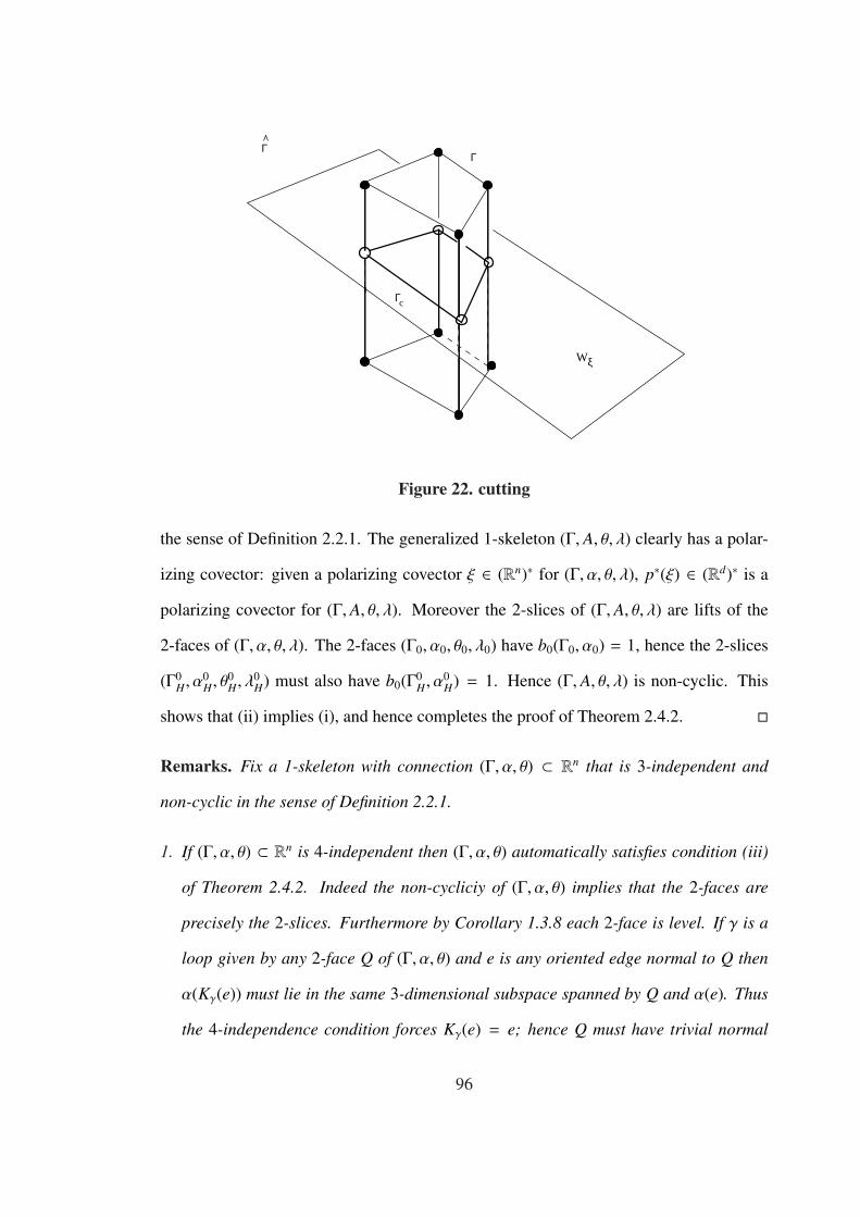
Γ

Γc

Wξ

Γ

Figure 22. cutting

the sense of Definition 2.2.1. The generalized 1-skeleton (Γ, A, θ, λ) clearly has a polar-

izing covector: given a polarizing covector ξ ∈ (Rn)∗ for (Γ, α, θ, λ), p∗(ξ) ∈ (Rd)∗ is a

polarizing covector for (Γ, A, θ, λ). Moreover the 2-slices of (Γ, A, θ, λ) are lifts of the

2-faces of (Γ, α, θ, λ). The 2-faces (Γ0, α0, θ0, λ0) have b0(Γ0, α0) = 1, hence the 2-slices

(Γ0H, α

0H, θ

0H, λ

0H) must also have b0(Γ0

H, α0H) = 1. Hence (Γ, A, θ, λ) is non-cyclic. This

shows that (ii) implies (i), and hence completes the proof of Theorem 2.4.2. �

Remarks. Fix a 1-skeleton with connection (Γ, α, θ) ⊂ Rn that is 3-independent and

non-cyclic in the sense of Definition 2.2.1.

1. If (Γ, α, θ) ⊂ Rn is 4-independent then (Γ, α, θ) automatically satisfies condition (iii)

of Theorem 2.4.2. Indeed the non-cycliciy of (Γ, α, θ) implies that the 2-faces are

precisely the 2-slices. Furthermore by Corollary 1.3.8 each 2-face is level. If γ is a

loop given by any 2-face Q of (Γ, α, θ) and e is any oriented edge normal to Q then

α(Kγ(e)) must lie in the same 3-dimensional subspace spanned by Q and α(e). Thus

the 4-independence condition forces Kγ(e) = e; hence Q must have trivial normal

96

holonomy. The somewhat surprising conclusion is: Any 4-independent non-cyclic

1-skeleton has a non-cyclic lift.

2. Without 4-independence (but still assuming 3-independence) our result says that if all

of the 2-slices of (Γ, α, θ) ⊂ Rn have trivial normal holonomy then (Γ, α, θ) satisfies

(iii). Thus we have a purely combinatorial criterion for checking if a 3-independent

non-cyclic 1-skeleton lifts: A 3-independent non-cyclic 1-skeleton has a non-cyclic

lift if and only if all of its 2-slices have trivial normal holonomy.

We have the following corollary of Theorem 2.4.2. For convenience we shall say that

a 1-skeleton has the lifting package if it satisfies condition (iii) in Theorem 2.4.2.

Corollary 2.4.9. Suppose the d-valent 1-skeleton (Γ, α, θ) ⊂ Rn has

i. the lifting package and

ii. an embedding f : VΓ → Rn.

Then (Γ, α, θ) ⊂ Rn is a projected simple polytope.

Proof. Theorem 2.4.2 implies that (Γ, α, θ, λ) ⊂ Rn has a non-cyclic lift (Γ, A, θ, λ) ⊂ Rd.

Thus by Theorem 2.1.5 it suffices to show that (Γ, A, θ, λ) admits an embedding F : VΓ →Rd. A result of Guillemin and Zara (see chapter 3, Theorem 3.1.14) implies that the map

π∗ : H(Γ, A) → H(Γ, α) induced by the projection morphism π : (Γ, α, θ) → (Γ, A, θ) is

surjective. Hence there is an equivariant class F ∈ H1(Γ, A, θ) such that π∗(F) = f . For

every oriented edge vw ∈ EΓ we have

F(w) − F(v) = c · A(vw),

for some c ∈ R. On the other hand we necessarily have

p(F(w)) − p(F(v)) = c · p(A(vw) = c · α(vw) = f (w) − f (v)

hence c > 0. This shows that F is an embedding of (Γ, A, θ). �

97

We end this chapter with some examples.

In Figure 23 we see a problem after passing over the first critical point. The down

cross-section lifts as Lemma 2.4.7 tells us, but the up cross-section has the wrong con-

nection to lift. The problem here is that the (triangular) 2-faces fail to have trivial normal

holonomy.

q1

q2

q3

q4

Wξ

p

ξ

Figure 23. A 3-Independent 1-Skeleton That Does Not Lift.

The 1-skeleton in R2 shown in Figure 24 also does not admit a lift (this is easy to see

without Theorem 2.4.2: if it did have a lift then it would be the projection of some (sim-

ple) 3-polytope which is impossible by Steinitz’ theorem (the graph is not 3-connected)).

However we see that this 1-skeleton has enough 2-faces (the four outer triangles and the

outer and inner hexagons), and these 2-faces all have trivial normal holonomy. The prob-

lem in this example is that the triangles fail to be level. One indication of this is that the

lines spanned by the directions assigned to the normal edges of a triangle do not meet in

a point.

98

Figure 24. reducible 1-skeleton, 2-faces not straight .

2.5 Concluding Remarks

We have the following problem:

Problem. When is a given d-valent 1-skeleton with connection (Γ, α, θ) ⊂ Rn a projection

of a (-n effective) 1-skeleton with connection (Γ, A, θ) ⊂ RN for n < N ≤ d?

Theorem 2.4.2 solves this problem for non-cyclic (Γ, A, θ) ⊂ Rd. Otherwise the prob-

lem is wide open.

In lifting problems of the above type, one is reminded of Steinitz’ Theorem:

Theorem 2.5.1. A simple graph G is the graph of a 3-dimensional polytope P ⊂ R3 if

and only if G is planar and 3-connected.

In some sense, Theorem 2.5.1 is much stronger than Corollary 2.4.9. Indeed in the

statement of Theorem 2.5.1 we are starting with a purely combinatorial object having no

geometric structure at all, and producing a convex 3-polytope. Also Theorem 2.5.1 does

not require P to be simple; the result holds for all 3-dimensional polytopes. On the other

hand, while Corollary 2.4.9 holds for any d ≥ 3, we require our polytopes to be simple

and the objects that we start out with already have some geometric strucutre.

However Theorem 2.5.1 can be proved in the same spirit as the proof of Theorem 2.4.2

(and hence also Corollary 2.4.9). Indeed one first introduces basic invertible operations

99

on planar, 3-connected simple graphs that preserve the lifting property: if the graph

lifts before the operation, then it lifts after the operation and vice-versa. In the proof of

Theorem 2.4.2 these operations are the blow-up and blow-down. One then shows how

to use these operations to transform the given graph into a “simpler” graph. In our case

this is the cutting technique. One then shows that this simpler graph has a lift. This is

analogous to our Lemma 2.4.6. See [29] chapter 4 for a proof of Theorem 2.5.1 along

these lines. Another nice reference for Theorem 2.5.1 (and 3-polytopes in general) is

Grunbaum’s book [11].

Crapo and Whiteley give another proof of Theorem 2.5.1 where the graph is given as

a bar-joint framework in R2. If a 1-skeleton (Γ, α) admits an embedding f : VΓ → Rn,

then one gets a bar-joint framework on the graph Γ using f . In [6], Crapo and White-

ley use ideas from rigidity theory to detect which planar bar-joint frameworks arise as

projections of 3-polytopes (and more general “polyhedral surfaces”). To my knowledge

there is not much known regarding lifting bar-joint frameworks in higher dimensions.

Question. Does Theorem 2.4.2 have a direct translation in terms of rigidity theory?

Does it already have an analogue in rigidity theory?

Another general question is “Can these techniques be used to obtain results in geom-

etry?”. A couple of problems in this direction are as follows.

Question. When does the T-action on a GKM T-manifold M, extend to a larger T -

action?

If we restrict the T -action of a GKM T -manifold, M, to the action by a sub-torus T0

such that the restricted action also satisfies GKM 1 and GKM 2 (from Definition 1.7.4),

then M becomes a GKM T0-manifold. The 1-skeleton for M with its restricted action

of T0 is exactly the projection of the 1-skeleton of M with its larger T -action via the

100

restriction map p : t∗ → t∗0. Requiring T to preserve a (non-degenerate) 2-form on M

enforces the restriction dim(T ) ≤ 12 dim(M) B d.

If M is a symplectic manifold and the T -action is Hamiltonian, there is a moment

map µ : M → t∗ such that the image of the 0-and 1-dimensional orbits is the 1-skeleton

associated to the GKM T -manifold M. In the case where M is a symplectic manifold

and the T -action is Hamiltonian with dim(T ) = d, M is called a toric manifold.

We can ask the following specialized question:

Question 1. Given a symplectic manifold (M, ω) of dim(M) = 2d admitting a Hamil-

tonian torus action via T = (S 1)n for n < d under what conditions is M actually a

toric manifold such that the T-action on M is actually the restriction of this larger torus

action?

The blow-up, reduction and cutting operations described above all have analogues in

symplectic geometry. Therefore one might conjecture that an analogue of Theorem 2.4.2

holds for symplectic, Hamiltonian T -manifolds.

Conjecture 1. A symplectic manifold (M, ω) of dim(M) = 2d admitting a Hamiltonian

torus action via T = (S 1)n for 1 < n < d is a toric manifold and the T-action the

restriction of this larger action if and only if all of the reduced spaces of M are toric

manifolds (orbifolds?).

Another interesting question is

Question 2. Which 1-skeleta come from GKM T-manifolds?

In [14], Guillemin and Zara showed that every GKM 1-skeleton satisfying certain

integrality conditions comes from a certain non-compact GKM T -manifold.

A Delzant polytope in Rd is a simple d-polytope whose edge directions span generate

the lattice Zd ⊂ Rd. Delzant shows in [7] that every Delzant polytope in Rd is the

101

moment map image of some 2d-dimensional toric manifold (see also [15]). In particular,

this implies that 1-skeleta of Delzant polytopes are the 1-skeleta toric manifolds. Then

determining which 1-skeleta are projections of 1-skeleta of Delzant polytopes would

yield a larger family of 1-skeleta coming from GKM T -manifolds.

Problem 2. Which 1-skeleta are projections of 1-skeleta of Delzant polytopes?

Corollary 2.4.9 determines the class of 1-skeleta coming from projections of arbitrary

simple polytopes. What additional conditions can we impose to determine projections of

the Delzant polytopes?

102

C H A P T E R 3

MORSE PROPERTIES

We now turn our attention to the cohomology rings associated to a 1-skeleton. In this

chapter we investigate the S -module structure of the equivariant cohomology ring. In

particular we are interested in 1-skeleta whose equivariant cohomology is a free module

over the polynomial ring S . In a series of papers [13], [14] and [16] Guillemin and Zara

studied 1-skeleta whose equivariant cohomology is free and admits a triangular basis

with respect to vertex orderings induced by polarizations. 1-skeleta satisfying such con-

ditions are said to have the Morse package. Guillemin and Zara, in [16] were successful

in classifying GKM 1-skeleta with the Morse package modulo planar 1-skeleta, using

the same reduction and cutting methods as we used in chapter 2. It turns out that their

classification result also holds for arbitrary straight 1-skeleta. In this chapter we pick

up where they leave off in some sense; we try to shed some light on the class of planar

1-skeleta that have the Morse package. It turns out that in the planar 3-valent case, the

Morse package coincides with straightness. Things are more complicated in the higher

valency cases. In fact one can construct infinite families of symmetric straight planar

1-skeleta some of which have the Morse package and some of which do not.

This chapter is divided into three sections. In Section 1 we define the Morse package

and relate the different notions of straightness (from Definition 1.3.6) to existence of

certain equivariant cohomology classes and integrals with a localization formula. At the

103

end we state the Guillemin-Zara classifiction result. In Section 2 we focus on planar 1-

skeleta. First we classify those 3-valent 1-skeleta which have the Morse package. As an

application of this result, we construct an infinite family of 3-valent planar 1-skeleta that

have the Morse package. Next we construct an infinite family of higher valency planar

1-skeleta equipped with a dihedral symmetry group. We then show that an infinite sub-

family of these has the Morse package. In Section 3 we give a few concluding remarks.

3.1 The Morse Package

In this section we fix a d-valent non-cyclic (in the sense of Definition 2.2.1) 1-skeleton

with connection (Γ, α, θ) ⊂ Rn; when the connection is irrelevant we will omit it and just

write (Γ, α). We also fix a polarizing covector ξ ∈ (Rn)∗ and a ξ-compatible Morse

function φ : VΓ → R.

It will be convenient to think of the acyclic orientation on Γ induced by ξ as giving a

partial ordering on the vertex set VΓ as follows: we say that v � w if there is a ξ-oriented

path from v to w in Γ. We also have a total ordering induced by φ: v ≤ w if φ(v) ≤ φ(w).

For each vertex p ∈ VΓ set

Fp B {q ∈ VΓ | p � q}

and

Fp B {q ∈ VΓ | p ≤ q}.

For each p ∈ VΓ, set

E+p B {e ∈ Ep | 〈ξ, α(e)〉 > 0}

the “Up”-oriented edges at p and

E−p B {e ∈ Ep | 〈ξ, α(e)〉 < 0}

104

the “Down”-oriented edges at p.

Definition 3.1.1. ([14],[16]) A homogeneous equivariant class τp ∈ H∗(Γ, α) is called a

generating class for p ∈ VΓ if it satisfies the following properties:

1. τp(p) =∏

e∈E−p α(e) and

2. supp(τp) ⊂ Fp.

We say that (Γ, α) admits a generating family if every vertex admits a generating class;

i.e. if there is a family of classes

{τp}p∈VΓ⊂ H(Γ, α)

where τp is a generating class for p.

By relaxing the support conditions we obtain a slightly more general family of classes

that are sometimes easier to produce.

Definition 3.1.2. A homogeneous equivariant class τp ∈ H∗(Γ, α) is called a pseudo-

generating class if it satisfies the following properties:

1. τp(p) =∏

e∈E−p α(e) and

2. supp(τp) ⊂ Fp.

We say that (Γ, α) admits a pseudo-generating family if every vertex admits a pseudo-

generating class; i.e. if there is a family of classes

{τp}p∈VΓ⊂ H(Γ, α)

where τp is a pseudo-generating class for p.

105

Let VΓ = {p1, . . . , pN} be the vertices labelled according to the total ordering, so that

pi < p j if i < j. Define for 1 ≤ i ≤ N the subspace

Hi B { f ∈ H(Γ, α) | supp( f ) ⊂ Fpi}.

This defines a finite S -module filtration of the equivariant cohomology ring of (Γ, α)

0 = HN ⊂ HN−1 ⊂ · · · ⊂ H2 ⊂ H1 = H(Γ, α).

For each 1 ≤ i ≤ N and each k ≥ 0 there are exact sequences of R-vector spaces

0 // Hki+1

ιi // Hki

εpi //∏

e∈E−piα(e) · S k−σ(pi) (3.1.1)

where ιi is the natural inclusion and εpi is evaluation at vertex pi and σ(p) B indξ(p).

Note that any class τ ∈ Hi such that εpi(τ) =∏

e∈E−piα(e) · 1 is a pseudo-generating class

for pi.

Exactness in (3.1.1) gives the family of inequalities

dimR(Hki ) − dimR(Hk

i+1) ≤ µk−σ(pi), (3.1.2)

for k ≥ 0 and for 1 ≤ i ≤ N, where

µ j B dimR S j =

(n + j − 1

j

).

Summing these inequalities from i = 1 to i = N − 1 yields the inequality

dimR(Hk(Γ, α)) ≤d∑

i=1

bi(Γ, α)µk−i (3.1.3)

for all k.

Lemma 3.1.3. ([14]) The following are equivalent:

i. (Γ, α) ⊂ Rn admits a generating family

ii. (Γ, α) ⊂ Rn admits a pseudo-generating family

106

iii. dimR(Hk(Γ, α)) =∑d

i=1 bi(Γ, α)µk−i for all k.

Proof. In the short exact sequence (3.1.1), the evaluation map εpi is surjective if and only

if there is a pseudo-generating class τpi ∈ Hi for pi. In other words (ii) is equivalent to

the sequence

0 // Hi+1ιi // Hi

εpi //∏

e∈E−p α(e) · S // 0. (3.1.4)

being exact. Exactness in (3.1.4) implies that the inequalities in (3.1.2), and thus also in

(3.1.3) are all equalities. This shows that (ii) implies (iii). Conversely suppose that (iii)

holds. In light of (3.1.3), we see that the only way this could happen is if the inequlities

in (3.1.2) are actually equalities. But this implies together with the exactness of (3.1.1)

that (3.1.4) is exact on the right, hence (ii) holds.

Now we will show the equivalence of (i) and (ii). One direction is obvious: since

Fp ⊂ Fp for every vertex p ∈ VΓ, a generating class is a pseudo-generating class, hence

(i) implies (ii). Conversely assume that there is a pseudo-generating class for every vertex

of Γ. We will show that there is a generating class for every vertex of Γ. Fix p ∈ VΓ and

let τp ∈ H∗(Γ, α) be a pseudo-generating class for p. Let q ∈ (Fp \ Fp) ∩ supp(τp) be the

smallest vertex. Then we must have that

τp(q) = K ·∏

e∈E−q

α(e)

for some non-zero K ∈ S . Let τq ∈ H(Γ, α) be a pseudo-generating class for q. Define

τp B τp − Kτq.

Then τp ∈ H(Γ, α) has

τp(p) =∏

e∈E−p

α(e)

and

supp(τp) ⊂ Fp

107

and the smallest vertex in the set

(Fp \ Fp) ∩ supp(τp)

is larger than the smallest vertex in

(Fp \ Fp) ∩ supp(τp).

This procedure will clearly terminate since there are only finitely many vertices, and

when it does we will be left with a class τp ∈ H∗(Γ, α) such that

τp(p) =∏

e∈E−p

α(e)

and

(Fp \ Fp) ∩ supp(τp) = ∅ :

since supp(τp) ⊂ Fp, the class τp must be a generating class for p. This shows that (ii) is

equivalent to (i), and hence completes the proof of Lemma 3.1.3. �

Definition 3.1.4. (Γ, α) ⊂ Rn has the Morse package if it satisfies any of the conditions

in Lemma 3.1.3.

Proposition 3.1.5. If (Γ, α) ⊂ Rn has the Morse package, then H(Γ, α) is a free S -

module.

Proof. Let {τp}p∈VΓbe a generating family for (Γ, α). We will show that these classes are

an S -basis for H(Γ, α).

First let us show that they generate H(Γ, α): For any homogeneous class f ∈ H(Γ, α)

define the height of f to be the smallest vertex h( f ) (with respect to “≤”) in supp( f ).

We prove that every homogeneous class f ∈ H(Γ, α) is in the S -span of {τp}p∈VΓby

downward induction on the h( f ).

108

If h( f ) is the maximum, then f evaluate to zero on all the neighbors of h( f ), hence

f (h( f )) must be divisible by∏

i(e)=h( f ) α(e). This implies that the class f is an S -multiple

of the class τh( f ). This is the base case.

Now assuming the assertion holds for classes f ′ with h( f ′) > q ∈ VΓ, let f be a

homogeneous class with h( f ) = q. For each vertex x ∈ VΓ such that qx ∈ E−q we

necessarily have f (x) = 0 since x < q. Therefore there is an element cq ∈ S such that

f (q) = cq · τq(q). Thus f = f − cqτq is a homogeneous class with h( f ) < h( f ). Therefore

by induction, f and therefore f lie in the S -span of {τp}p∈VΓ.

Now we will show that the generating classes are S -linearly independent. Suppose

there is a non-trivial dependence relation

∑

p∈VΓ

cpτp, cp ∈ S (3.1.5)

Let q ∈ VΓ be the smallest vertex such that cq , 0. Note that for p > q, τp(q) = 0. Hence

evaluating (3.1.5) at q yields cqτq(q) = 0 which implies that cq = 0, a contradiction.

Therefore there is no non-trivial dependence relation among the {τp}p∈VΓ, hence they are

S linearly independent. This completes the proof of Proposition 3.1.5. �

Remark. This notion of the “Morse package of a 1-skeleton” was invented by Guillemin

and Zara and seems to have evolved out of the series of papers [13],[14] and [16]

although the term itself only appears in [16]. The argument in the proof of Lemma 3.1.3

is essentially the one given by Guillemin and Zara in [14]. Definition 3.1.4 appears

in [16], although in that paper they make the blanket assumption that all 1-skeleta are

GKM.

109

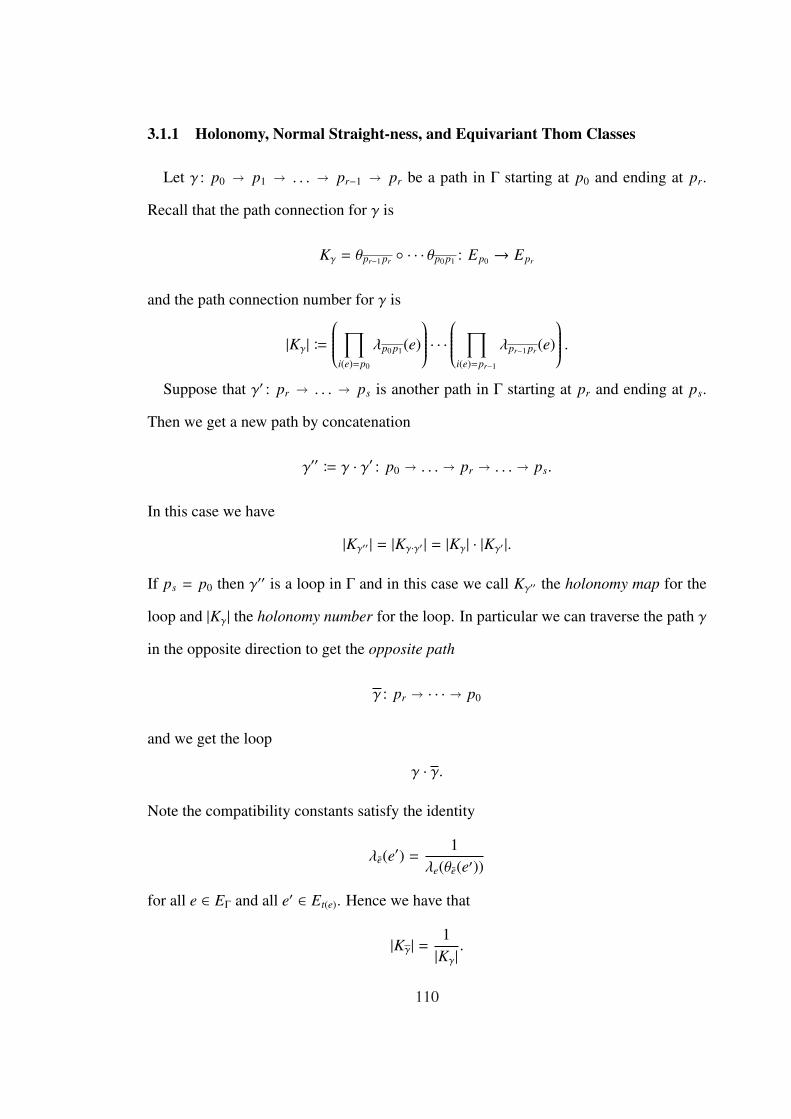
3.1.1 Holonomy, Normal Straight-ness, and Equivariant Thom Classes

Let γ : p0 � p1 � . . . � pr−1 � pr be a path in Γ starting at p0 and ending at pr.

Recall that the path connection for γ is

Kγ = θpr−1 pr ◦ · · · θp0 p1 : Ep0 → Epr

and the path connection number for γ is

|Kγ| B∏

i(e)=p0

λp0 p1(e)

· · ·

∏

i(e)=pr−1

λpr−1 pr (e)

.

Suppose that γ′ : pr � . . . � ps is another path in Γ starting at pr and ending at ps.

Then we get a new path by concatenation

γ′′ B γ · γ′ : p0 � . . . � pr � . . . � ps.

In this case we have

|Kγ′′ | = |Kγ·γ′ | = |Kγ| · |Kγ′ |.

If ps = p0 then γ′′ is a loop in Γ and in this case we call Kγ′′ the holonomy map for the

loop and |Kγ| the holonomy number for the loop. In particular we can traverse the path γ

in the opposite direction to get the opposite path

γ : pr � · · · � p0

and we get the loop

γ · γ.

Note the compatibility constants satisfy the identity

λe(e′) =1

λe(θe(e′))

for all e ∈ EΓ and all e′ ∈ Et(e). Hence we have that

|Kγ| = 1|Kγ| .

110

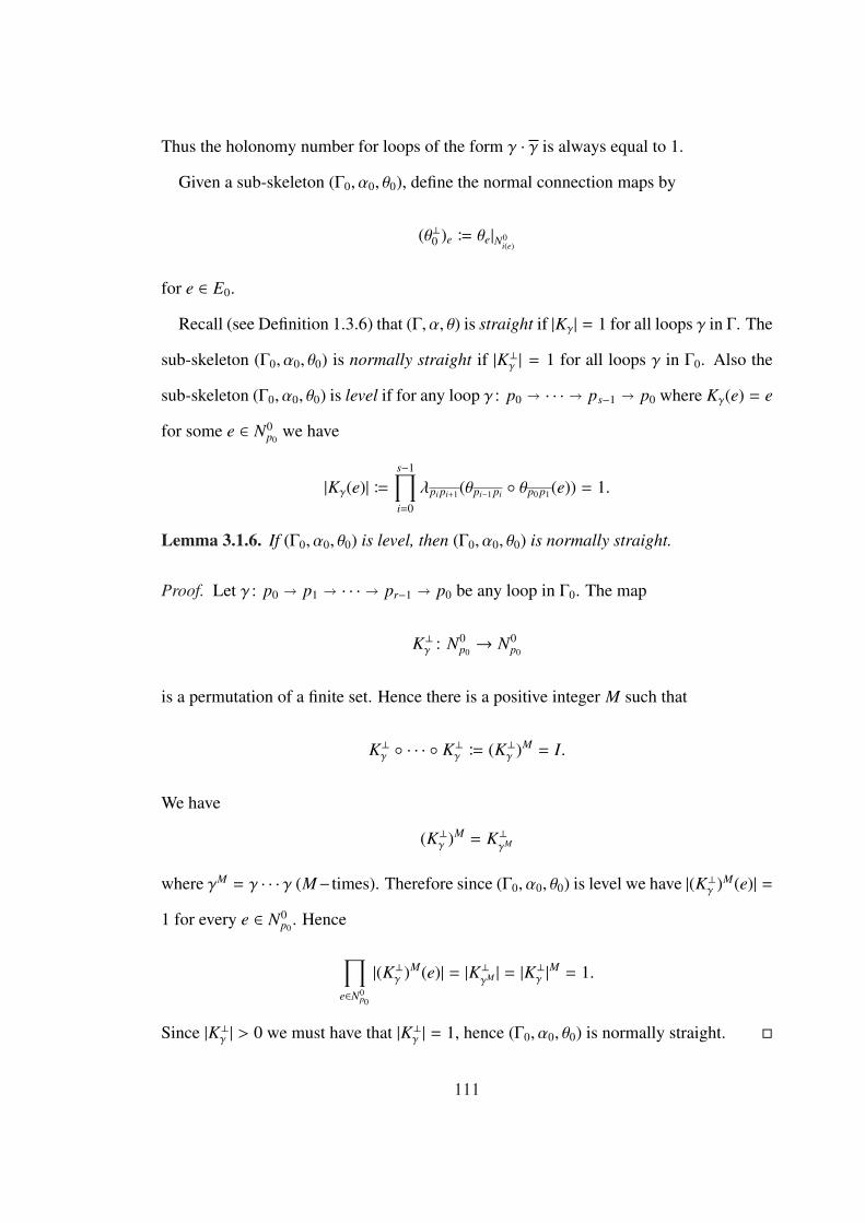
Thus the holonomy number for loops of the form γ · γ is always equal to 1.

Given a sub-skeleton (Γ0, α0, θ0), define the normal connection maps by

(θ⊥0 )e B θe|N0i(e)

for e ∈ E0.

Recall (see Definition 1.3.6) that (Γ, α, θ) is straight if |Kγ| = 1 for all loops γ in Γ. The

sub-skeleton (Γ0, α0, θ0) is normally straight if |K⊥γ | = 1 for all loops γ in Γ0. Also the

sub-skeleton (Γ0, α0, θ0) is level if for any loop γ : p0 � · · · � ps−1 � p0 where Kγ(e) = e

for some e ∈ N0p0

we have

|Kγ(e)| Bs−1∏

i=0

λpi pi+1(θpi−1 pi ◦ θp0 p1(e)) = 1.

Lemma 3.1.6. If (Γ0, α0, θ0) is level, then (Γ0, α0, θ0) is normally straight.

Proof. Let γ : p0 � p1 � · · · � pr−1 � p0 be any loop in Γ0. The map

K⊥γ : N0p0→ N0

p0

is a permutation of a finite set. Hence there is a positive integer M such that

K⊥γ ◦ · · · ◦ K⊥γ B (K⊥γ )M = I.

We have

(K⊥γ )M = K⊥γM

where γM = γ · · · γ (M− times). Therefore since (Γ0, α0, θ0) is level we have |(K⊥γ )M(e)| =1 for every e ∈ N0

p0. Hence

∏

e∈N0p0

|(K⊥γ )M(e)| = |K⊥γM | = |K⊥γ |M = 1.

Since |K⊥γ | > 0 we must have that |K⊥γ | = 1, hence (Γ0, α0, θ0) is normally straight. �

111

Proposition 3.1.7. Let (Γ0, α0, θ0) ⊂ (Γ, α, θ) be a totally geodesic sub-skeleton. Then

(Γ0, α0, θ0) has a Thom class if and only if (Γ0, α0, θ0) is normally straight.

Proof. Assume that (Γ0, α0, θ0) is normally straight. Fix a vertex p0 ∈ V0. We will define

a function τ0 : VΓ → S as follows.

To define τ0 on {p0} t (VΓ \ V0) set

τ0(q) =

∏e∈N0

p0α(e) if q = p0

0 if q < V0

For pr ∈ V0 let γr : p0 � · · · � pr be any path in Γ0 and define

τ(pr) B |K⊥γr|∏

e∈N0pr

α(e).

Since (Γ0, α0, θ0) is normally straight, this value is independent of the path γr: if γ′r : p0 �· · · � pr is another path in Γ0, then γr · γ′r : p0 � · · · � p0 is a loop, hence

|K⊥γr| · |K⊥

γ′r| = |K

⊥γr|

|K⊥γ′r| = 1.

Consequently, the function thus defined is an equivariant class on (Γ, α, θ). Indeed sup-

pose that pr ps ∈ E0 is an edge. We have

τ0(pr) = |K⊥γr|∏

e∈N0pr

α(e)

and

τ0(ps) = |K⊥γs|∏

e∈N0ps

α(e).

But we can take path γs to be the path

γs = γ · {pr � ps} : p0 � · · · � pr � ps,

hence we see that

|K⊥γs| = |K⊥γr

| ·∏

e∈N0pr

λpr ps(e)

,

112

thus τ0(pr) − τ0(ps) ≡ 0 mod α(pr ps).

Conversely, assume that (Γ0, α0, θ0) supports a Thom class, τ0 : VΓ → S . For each

p ∈ V0 there is a positive constant cp ∈ R+ such that

τ0(p) = cp

∏

e∈N0p

α(e).

Since τ0 is an equivariant class, these constants must satisfy the following condition: For

each pq ∈ E0,cq

cp=

∏

e∈N0p

λpq(e).

Now let γ : p0 � p1 � · · · � pr−1 � p0 be any loop in Γ0. Then we must have

|K⊥γ | =cp1

cp0

· · · cp0

cpr−1

= 1

hence (Γ0, α0, θ0) is normally straight. This completes the proof of Proposition 3.1.7. �

Recall that given a k-dimensional sub-space H ⊂ Rn, and a vertex p ∈ VΓ, there

is a unique maximal totally geodesic sub-skeleton (Γ0H, α

0H, θ

0H) containing p such that

α0H(E0

H) ⊂ H, called the k-slice corresponding to H at p of (Γ, α, θ). We have the follow-

ing corollary of Proposition 3.1.7.

Corollary 3.1.8. Every k-slice has a Thom class.

Proof. By Theorem 1.3.8 in chapter 1 every k-slice is level. By Lemma 3.1.3 every

k-slice is also normally straight. Thus by Proposition 3.1.7, every k-slice has a Thom

class. �

Other sub-skeleta that always admit Thom classes are the 0- and 1-valent sub-skeleta;

that is the vertices and edges of Γ, respectively. Given p ∈ VΓ, and any non-zero constant

C ∈ R define the function

τp : VΓ → S d

113

by

τp(q) =

C∏

e∈Epα(e) if q = p

0 if q , p.

We call τp a top-class at p. We say that τp is a non-vanishing top-class if τp , 0 in

H(Γ, α). The non-vanishing top classes will play an important role in the sequel, when

we discuss integrals with localization formulae.

For e = pq ∈ EΓ define the function

σe : VΓ → S d−1

σe(x) =

∏e∈Ep\pq α(e) if x = p

∏e∈Ep

λpq(e)∏

e∈Ep\pq α(θpq(e)) if x = q

0 if x , p, q

Then σe is a homogeneous class of degree (d − 1) with supp(σe) = {p, q}, hence it is a

Thom class for e. We will refer to σe as the edge-class of e.

3.1.2 Straight-ness, Top Classes, and Localization

Definition 3.1.9. An integral on (Γ, α, θ) is any non-zero graded S -module homomor-

phism ∫

Γ

: H(Γ, α)→ S [d].

We say the integral has a localization formula if there exist constants {cp}p∈VΓ⊂ R+ such

that ∫

Γ

f =∑

p∈VΓ

f (p)cp

∏i(e)=p α(e)

.

The important point here is that the sum

∑

p∈VΓ

f (p)cp

∏i(e)=p α(e)

lies in S and not just in the field of fractions Q(S ).

114

Proposition 3.1.10. The following are equivalent:

A. (Γ, α, θ) has an integral with a localization formula

B. (Γ, α, θ) has a non-vanishing top-class

C. (Γ, α, θ) is straight.

Proof. (A⇒B):

Assume that (Γ, α) has an integral with localization formula. Let τp ∈ Hd(Γ, α) be the

class defined by

τp(q) =

∏i(e)=p α(e) if q = p

0 if q , p.(3.1.6)

Then ∫

Γ

τp =∑

q∈VΓ

τp(q)cq

∏i(e)=q α(e)

=1cp, 0.

Since∫

Γis an S -module homomorphism, the class in ordinary cohomology τp ∈ H(Γ, α)

must be non-zero.

(B⇒C):

Assume that (Γ, α) has a non-vanishing top-class τ ∈ Hd(Γ, α). Suppose that supp(τ) =

{p}. We may assume after possibly re-scaling that τ : VΓ → S d is defined by (3.1.6).

Let

γ : p0 � p1 � · · · � pr � p0

be any loop. We would like to show that |Kγ| = 1. Let γi be the path along γ from p to

pi:

γi : p0 � p1 � · · · � pi.

Thus γr+1 = γ is the whole loop. For each 1 ≤ i ≤ r + 1, denote by σi the edge-class

σpi−1 pi ∈ Hd−1(Γ, α). Define

τ1 B α(p1 p0) · σ1 + τ

115

and inductively define

τi B |Kγi−1 |α(pi pi−1) · σi + τi−1. (3.1.7)

Since

|Kγi | =∏

e∈Epi−1

λpi−1 pi(e)|Kγi−1 |, (3.1.8)

we can explicitly compute τi:

τi(q) =

|Kγi |∏

i(e)=piα(e) if q = pi

0 if q , pi.

Note that supp(τi) = {pi} and that τi = τ for all 1 ≤ i ≤ r + 1, by (3.1.7). On the other

hand we have

τr+1(q) =

|Kγ|∏i(e)=p α(e) if q = p

0 if q , p

hence τr+1 = |Kγ|τ. But τr+1 = τ, hence |Kγ| = 1, and this proves that (Γ, α, θ) is

straight.

(C⇒A):

Assume that (Γ, α) is straight. Fix a basepoint p ∈ VΓ. Set cp = 1. For a different

vertex q, let γq : p � p1 � · · · � pk � q be any path from p to q and define cq = |Kγq |.Note that if

γ′q : p � p′1 � · · · � p′m � q

is another path from p to q, then

γ B γq · γ′q : p � · · · � pk � q � p′m � · · · � p

is a loop based at p and

|Kγ| = |Kγq | · |Kγ′q| = |Kγq | ·

1|Kγ′q |

.

116

Since (Γ, α, θ) is straight |Kγ| = 1, so we have |Kγq | = |Kγ′q |. Hence cq is independent of

the path γq chosen. Consequently, for any edge pq ∈ Ep we have that

cq

cp=

∏

e∈Ep

λpq(e),

by (3.1.8).

Now we want to show that for this choice of constants {cp}p∈VΓ, the sum

∑

p∈VΓ

f (p)cp

∏i(e)=p α(e)

(3.1.9)

is in S for every homogeneous equivariant class f ∈ Hk(Γ, α). The following argument

is due to Guillemin and Zara ([13]).

By finding the least common denominator we can write the sum in (3.1.9) as

g∏Ni=1 αi

where {αi}Ni=1 is a complete list of all of the directions that occur in the denominators in

(3.1.9) and {αi}Ni=1 is pairwise linearly independent and g ∈ S . We will show that for any

i, αi divides g.

We can partition VΓ into two disjoint subsets:

V1Γ = {q ∈ VΓ | there is e ∈ Eq with α(e) = Kαi}

and

V2Γ = VΓ \ V1

Γ .

We write the sum in (3.1.9) as

∑

p∈VΓ

f (p)cp

∏i(e)=p α(e)

=∑

p∈V1Γ

f (p)cp

∏i(e)=p α(e)

+∑

p∈V2Γ

f (p)cp

∏i(e)=p α(e)

. (3.1.10)

Since αi is coprime with α(e) for each p ∈ V2Γ

and every e ∈ Ep, we can write the second

summand on the RHS of (3.1.10) as

∑

p∈V2Γ

f (p)cp

∏i(e)=p α(e)

=g2∏j,i α j

. (3.1.11)

117

For each p ∈ V1Γ

note that there is a unique vertex q ∈ V1Γ

such that pq ∈ EΓ and

α(pq) = Kαi for some K ∈ R. Write the set of such oriented edges as EiΓ. Then by

pairing terms we can write the first summand in (3.1.10) as

∑

p∈V1Γ

f (p)cp

∏i(e)=p α(e)

=12

∑

pq∈EiΓ

(f (p)

cp∏

i(e)=p α(e)+

f (q)cq

∏i(e′)=q α(e′)

). (3.1.12)

Consider a term in the sum on the RHS of (3.1.12). Finding a common denominator we

can write the “pq” term as

f (p)cq∏

e′,qp α(e′) − f (q)cp∏

e,pq α(e)cpcq

∏e,pq α(e)

∏e′,qp α(e′)α(pq)

. (3.1.13)

We can rewrite the numerator in (3.1.13) as

f (p)cq

∏

e,pq

α(θpq(e)) − f (q)cp

∏

e,pq

α(e). (3.1.14)

Recall that cq =∏

e∈Epλpq(e)cp and that

α(e) − λpq(e)α(θpq(e)) ≡ 0 mod α(pq).

Hence from (3.1.14) we get the equivalence

f (p)cq

∏

e,pq

α(θpq(e)) − f (q)cp

∏

e,pq

α(e) ≡ f (p)cp

∏

e,pq

α(e) − f (q)cp

∏

e,pq

α(e), (3.1.15)

and the RHS of (3.1.15) is divisible by α(pq) since f is an equivariant class. Hence the

sum on the RHS of (3.1.12) can be written

12

∑

pq∈EiΓ

(f (p)

cp∏

i(e)=p α(e)+

f (q)cq

∏i(e′)=q α(e′)

)=

12

∑

pq∈EiΓ

Gp,q

cpcq∏

e,pq α(e)∏

e′,qp α(e′)

(3.1.16)

for some Gp,q ∈ S . Now the main point is that the denominators of the summands on

the RHS are all co-prime to αi (since the sets α(Ep) and α(Eq) are each 2-independent).

Thus we can write (3.1.16) as

12

∑

pq∈EiΓ

Gp,q

cpcq∏

e,pq α(e)∏

e′,qp α(e′)=

g1∏j,i α j

. (3.1.17)

118

Hence combining (3.1.11) with (3.1.17) we can write

g∏Nj=1 α j

=g1∏j,i α j

+g2∏j,i α j

,

hence αi divides g for any i and hence

∑

p∈VΓ

f (p)cp

∏e∈Ep

α(e)

is in S . This completes the proof of Proposition 3.1.10. �

An important corollary of the proof of Proposition 3.1.10 is the following.

Corollary 3.1.11. (Γ, α, θ) is straight if and only if there exist positive constants, unique

up to scaling, {cp}p∈VΓ⊂ R+ such that whenever pq ∈ EΓ,

cq

cp=

∏

e∈Ep

λpq(e).

Remark. If (Γ, α) has the Morse package then it has a non-vanishing top-class; one such

class will be the generating class for the maximal vertex of VΓ (with respect to �). Hence

by Proposition 3.1.10, (Γ, α) will also have an integral with a localization formula.

We have already alluded to the fact that 1-skeleta of simple d-polytopes have the

Morse package. This fact is almost trivial for the d = 2 case; we state it as a lemma

here as we will refer to it later.

Lemma 3.1.12. Suppose that (Γ, α) ⊂ R2 is 2-valent. Then (Γ, α) has the Morse package.

Proof. Fix a polarizing covector ξ. Note that

bi(Γ, α) =

1 if i = 0, 2

|VP| − 2 if i = 1.

A generating class for the unique minimum of (Γ, α) (with respect to ξ) is given by the

constant function 1 ∈ H0(Γ, α) that assigns 1 to every vertex. A generating class for

119

the unique maximum is just a top-class supported at that vertex. Generating classes for

vertices v of index 1 is just given by the edge class of the unique edge directed upwards

at v. Hence (Γ, α) admits a generating family. �

The following proposition gives a useful criterion for checking the straightness of a

(non-cyclic) 1-skeleton.

Proposition 3.1.13. (Γ, α, θ) ⊂ Rn is straight if and only if every 2-slice (Γ0H, α

0H, θ

0H) is

straight.

Proof. First we check the easy direction: assume that (Γ, α, θ) is straight. Fix a 2-slice

(Γ0H, α

0H, θ

0H) and fix a loop γ in Γ0

H. Note that (Γ0H, α

0H, θ

0H) is normally straight by Lemma

3.1.6. Therefore the holonomy number for γ in Γ factors

|Kγ| = |K⊥γ | · |(K0H)γ| = 1.

Since |Kγ| = 1 and |K⊥γ | = 1 we must also have the |(K0H)γ| = 1, hence (Γ0

H, α0H, θ

0H) is

straight.

The other direction is a little more work. Assume that all the 2-slices are straight. Let

p be the unique mimimum of Γ with respect to the partial order induced by our fixed

polarizing covector ξ, and let γ : p � · · · � p be any loop in Γ based at p ∈ VΓ. We

want to show that |Kγ| = 1. Define the m-height of γ, to be the pair consisting of the

vertex h(γ) ∈ Vγ which is the largest vertex of γ (with respect to “≤”) and the number

µ(γ) ∈ Z≥0 which is the number of times the path γ passes through the vertex h(γ) (the

“multiplicity of h(γ) in γ). We endow the set VΓ × Z≥0 with the lexicographic ordering

(i.e. (p, n) ≤ (q,m) if and only if either p < q or p = q and n < m); this gives a total

ordering to the set of loops γ in Γ. We will prove that |Kγ| = 1 by induction on the

m-height of γ.

120

If h(γ) = p then γ must be the trivial loop (with no edges) hence |Kγ| = 1 by default.

This is the base case.

Suppose (h(γ), µ(γ)) = (rm, M) where

γ : p � r1 � . . . � rm−1 � rm � rm+1 � . . . � rk � p.

If rm−1 = rm+1 then we can factor the loop γ into γb · γm · γ f where

γb : p � r1 � . . . � rm−1,

and

γ f : rm+1 � rm+2 � . . . � rk � p,

and

γm : rm−1 � rm � rm+1.

But |Kγm | = 1; hence if

γ′ B γb · γ f

then γ′ is a loop based at p with either h(γ′) < rm = h(γ) or µ(γ′) = M − 1 < M = µ(γ),

and |Kγ′ | = |Kγ|. Thus by induction |Kγ′ | = 1 and we are done.

Otherwise rm−1 , rm+1. In this case let H = spanR{α(rmrm−1), α(rmrm+1)} ⊂ Rn and

let (Γ0H, α

0H, θ

0H) be the corresponding 2-slice containing rm. Let s0 ∈ V0

H be the unique

minimum in Γ0H with respect to the induced partial ordering on V0

H (the non-cyclicity of

(Γ, α, θ) implies that all 2-slices have a unique minimum). Then there exist ξ-oriented

paths

γ1 : s0 � t1 � . . . � ta � rm−1

γ2 : s0 � u1 � . . . � ub � rm+1.

Let

γb : p � r1 � . . . � rm−1,

121

γm : rm−1 � rm � rm+1,

and

γ f : rm+1 � . . . � rk � p.

Then

γ = γb · γm · γ f

and

|Kγ| = |Kγb | · |Kγm | · |Kγ f |.

γmγ1

γb

rk

γfr1

γ2

s

tr

p

0

t1

am

rm−1

rm+1

u1

ub

H

Figure 25. Decreasing the m-height of a loop on a 2-slice

By assumption we have that

|Kγ1 | · |Kγm | · |Kγ2 | = 1

hence we can replace γ by the new loop

γ = γb · γ1 · γ2 · γ f .

122

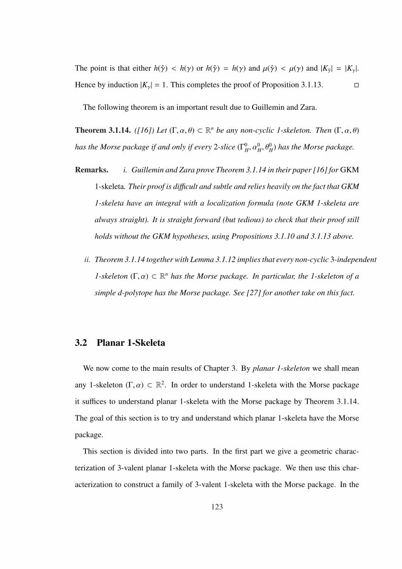
The point is that either h(γ) < h(γ) or h(γ) = h(γ) and µ(γ) < µ(γ) and |Kγ| = |Kγ|.Hence by induction |Kγ| = 1. This completes the proof of Proposition 3.1.13. �

The following theorem is an important result due to Guillemin and Zara.

Theorem 3.1.14. ([16]) Let (Γ, α, θ) ⊂ Rn be any non-cyclic 1-skeleton. Then (Γ, α, θ)

has the Morse package if and only if every 2-slice (Γ0H, α

0H, θ

0H) has the Morse package.

Remarks. i. Guillemin and Zara prove Theorem 3.1.14 in their paper [16] for GKM

1-skeleta. Their proof is difficult and subtle and relies heavily on the fact that GKM

1-skeleta have an integral with a localization formula (note GKM 1-skeleta are

always straight). It is straight forward (but tedious) to check that their proof still

holds without the GKM hypotheses, using Propositions 3.1.10 and 3.1.13 above.

ii. Theorem 3.1.14 together with Lemma 3.1.12 implies that every non-cyclic 3-independent

1-skeleton (Γ, α) ⊂ Rn has the Morse package. In particular, the 1-skeleton of a

simple d-polytope has the Morse package. See [27] for another take on this fact.

3.2 Planar 1-Skeleta

We now come to the main results of Chapter 3. By planar 1-skeleton we shall mean

any 1-skeleton (Γ, α) ⊂ R2. In order to understand 1-skeleta with the Morse package

it suffices to understand planar 1-skeleta with the Morse package by Theorem 3.1.14.

The goal of this section is to try and understand which planar 1-skeleta have the Morse

package.

This section is divided into two parts. In the first part we give a geometric charac-

terization of 3-valent planar 1-skeleta with the Morse package. We then use this char-

acterization to construct a family of 3-valent 1-skeleta with the Morse package. In the

123

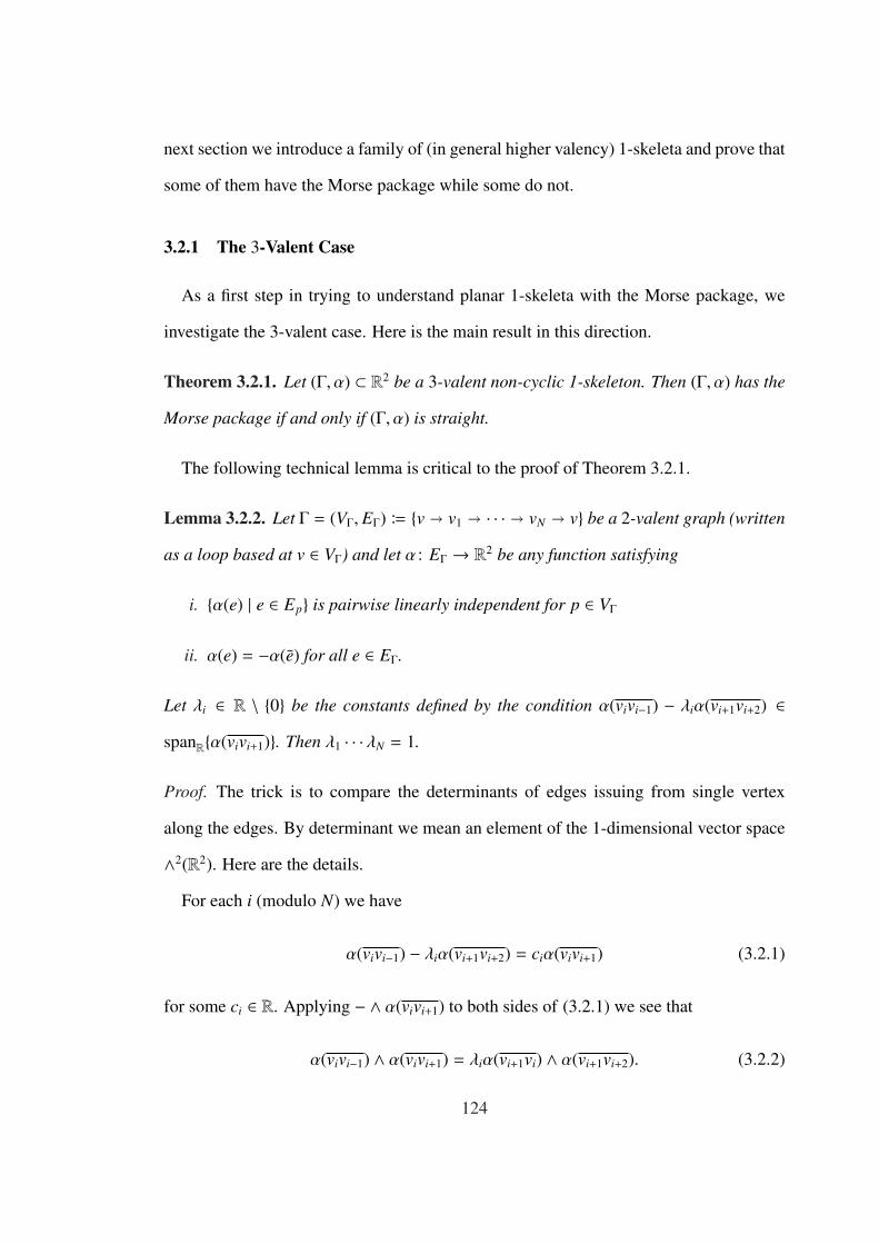
next section we introduce a family of (in general higher valency) 1-skeleta and prove that

some of them have the Morse package while some do not.

3.2.1 The 3-Valent Case

As a first step in trying to understand planar 1-skeleta with the Morse package, we

investigate the 3-valent case. Here is the main result in this direction.

Theorem 3.2.1. Let (Γ, α) ⊂ R2 be a 3-valent non-cyclic 1-skeleton. Then (Γ, α) has the

Morse package if and only if (Γ, α) is straight.

The following technical lemma is critical to the proof of Theorem 3.2.1.

Lemma 3.2.2. Let Γ = (VΓ, EΓ) B {v � v1 � · · · � vN � v} be a 2-valent graph (written

as a loop based at v ∈ VΓ) and let α : EΓ → R2 be any function satisfying

i. {α(e) | e ∈ Ep} is pairwise linearly independent for p ∈ VΓ

ii. α(e) = −α(e) for all e ∈ EΓ.

Let λi ∈ R \ {0} be the constants defined by the condition α(vivi−1) − λiα(vi+1vi+2) ∈spanR{α(vivi+1)}. Then λ1 · · · λN = 1.

Proof. The trick is to compare the determinants of edges issuing from single vertex

along the edges. By determinant we mean an element of the 1-dimensional vector space

∧2(R2). Here are the details.

For each i (modulo N) we have

α(vivi−1) − λiα(vi+1vi+2) = ciα(vivi+1) (3.2.1)

for some ci ∈ R. Applying − ∧ α(vivi+1) to both sides of (3.2.1) we see that

α(vivi−1) ∧ α(vivi+1) = λiα(vi+1vi) ∧ α(vi+1vi+2). (3.2.2)

124

Inductively we find that

α(vvN) ∧ α(vv1) = λ1 · · · λNα(vvN) ∧ α(vv1), (3.2.3)

hence λ1 · · · λN = 1 as desired. This completes the proof of Lemma 3.2.2. �

eN

i+1e

e2

v2 vN

1v

vi−1

vN−1

vi+1

vi

eN−2

ei

ei−1

e1

eN−1

vN−2

v

e

...

...

Figure 26. A “Thom-Class” on an arbitrary loop

We are now in a position to prove Theorem 3.2.1. Let (Γ, α) ⊂ R2 be a 3-valent,

non-cyclic 1-skeleton as in the statement of Theorem 3.2.1. Fix a polarizing covector

ξ ∈ (R2)∗.

125

Proof. of Theorem 3.2.1 One direction is trivial: assuming that (Γ, α) has the Morse

package, the generating class of the unique maximum (with respect to the partial order

induced on VΓ by ξ) is a non-vanishing top-class. By Proposition 3.1.10, (Γ, α) must be

straight.

Conversely, assume that (Γ, α) is straight. To show that (Γ, α) has the Morse package,

it suffices to show that every vertex of index 1 has a generating class. Fix a vertex v ∈ VΓ

with indξ(v) = 1. There exist two paths

γ1 : v � u1 � · · · � ur � x

and

γ2 : v � w1 � · · · � ws � x

that are ξ oriented and such that the sets {u1 . . . , ur} and {w1, . . . ,ws} are disjoint. Indeed

along either path, at the ith step we can either augment the path with an edge leading to

a higher vertex or we are at the unique highest vertex in which case we must stop. Both

paths must at least meet at this vertex. Then let x be the smallest vertex where both paths

meet. Let Γv = (VΓv , EΓv) denote the 2-valent graph defined to be the cycle formed by

concatenating γ1 and γ2. For notational convenience write

γ1 · γ2 : v � v1 � · · · � vN � v;

hence v1 = u1 and vN = ws.

Let λi ∈ R \ {0} be defined by

α(vivi−1) − λiα(vi+1vi+2) = ciα(vivi+1) (3.2.4)

for some ci ∈ R. For each vi ∈ γ1 · γ2 let ei ∈ Evi be the edge at vi normal to the subgraph

γ1 · γ2. Let λi ∈ R \ {0} be defined by

α(ei) − λiα(ei+1) = kiα(vivi+1) (3.2.5)

126

for some ki ∈ R.

Then for each 1 ≤ i ≤ N we have

α(vivi−1) · α(ei) ≡ (λiλi)α(vi+1vi+2) · α(ei+1) mod α(vivi+1). (3.2.6)

On the other hand we also have for 1 ≤ i ≤ N,

α(vivi−1) · α(ei) ≡ (λvivi+1(vivi−1)λvivi+1(ei))α(vi+1vi+2) · α(ei+1) mod α(vivi+1). (3.2.7)

Since the principal ideal generated by α(vivi+1) is prime in S , the ring S/〈α(vivi+1)〉 is an

integral domain, hence we conclude that

λiλi = λvivi+1(vivi−1)λvivi+1(ei). (3.2.8)

Since (Γ, α) is straight, (3.2.8) implies that λ1λ1 · · · λNλN = 1. By Lemma 3.2.2 we

also have that λ1 · · · λN = 1. Therefore we must have that λ1 · · · λN = 1. This implies that

the function τv : VΓ → S 1 defined by

τv(q) =

α(e) if q = v

(λi · · · λ1

)α(ei) if q = vi

0 otherwise

is actually an equivariant class. By construction, τv is a generating class for v. See

Figure 3.2.1; the arrows at the vertices (in bold font) denote the values of the class at the

vertices and the dotted line is meant to show that they “line up” to define a class.

This shows that (Γ, α) admits a generating family and thus completes the proof of

Theorem 3.2.1. �

As an application of Theorem 3.2.1 we give an infinite family of planar 3-valent 1-

skeleta that have the Morse package.

127

CS-1-Skeleta

A convex polygon P ⊂ R2 containing the origin in its interior is centrally symmetric if

x ∈ P implies −x ∈ P. Let P ⊂ R2 be any centrally symmetric polygon and ΓP = (V, E)

its 2-valent graph. Let ΓP = (V , E) denote the graph obtained from ΓP by joining anti-

podal vertices by edges; thus V = V and E = E t{v(−v) | v ∈ V

}. Define

αP : E → R2

by

αP(e) =

αP(e) if e ∈ E

−~v if e = v(−v)

(here we are taking αP : E → R2 to be the axial function on ΓP defined by the embedding

of P). Let θP denote the (unique) connection on (ΓP, αP). There is a unique connection

θP on ΓP such that θP|E = θP. It is straightforward to check that αP defines an axial

function for the pair (ΓP, θP). The 3-valent 1-skeleton with connection thus obtained

(ΓP, αP, θP) ⊂ R2 is called a CS-1-skeleton.

Theorem 3.2.3. CS-1-skeleta have the Morse package.

Proof. By Theorem 3.2.1 it suffices to show that all CS-1-skeleta are straight. By Corol-

lary 3.1.11 it suffices to show that there exist positive constants {cp}p∈V ⊂ R+ such that

for every pq ∈ EΓ we have

cq

cp=

∏

i(e)=p

λpq(e).

By Lemma 3.1.12 (ΓP, αP, θP) is straight hence by Corollary 3.1.11 there exist positive

constants {cp}p∈V ⊂ R+, unique up to scaling, such that for edges pq ∈ E,

cq

cp=

∏

e∈Ep

λpq(e) = λpq(e),

128

where e ∈ (EP)p is the unique oriented edge at p that is not pq. We choose these constants

such that cp = c−p for all p ∈ VP; we can do this by the central symmetry of P.

The claim is that this choice of constants for (ΓP, αP, θP) will also work for (ΓP, αP, θP).

There are two types of edges to check: edges of P and “central” edges.

i. Let pq ∈ EP. Then we have

α(p(−p)) = −~p

and

α(q(−q)) = −~q.

Hence λpq(p(−p)) = 1, hence

cq

cp=

∏

e∈Ep

λpq(e) · 1 =∏

e∈Ep

λpq(e)

ii. Now let p(−p) ∈ E be a “central” edge. If pq, pr ∈ Ep it follows that from central

symmetry that

λp(−p)(pq) · λp(−p)(pr) = λp(−p)(pq) · λ(−p)p(qp) = 1.

On the other hand we chose our constants so that cp = c−p, hence we have that

λp(−p)(pq) · λp(−p)(pr) = 1 =cp

c(−p).

See Figure 27.

This shows that (ΓP, αP, θP) is straight, hence has the Morse package by Theorem

3.2.1. �

As one might expect, things are more complicated in the higher valency cases.

129

p

−p

r

−q

−r

q

Figure 27. A CS-1-Skeleton

3.2.2 Crossed-Regular Polygons

Let P ⊂ R2 be a regular m-gon (centered at the origin) with symmetry group I(m)

(= the dihedral group generated by m reflections). Let ΓP = (VP, EP) denote the graph

of P and define the completion of P to be the complete graph, KP on the vertex set VP:

KP = (VP, XP) where the oriented edge set is XP = {pq | p, q ∈ VP}. For each (oriented)

edge e B pq ∈ XP let se ∈ I(m) denote the reflection across the line perpendicular to the

line segment joining p to q. Define the regular connection, θ = {θe}e∈XP , on KP by

(XP)pθe // (XP)q

pr // se(p)se(r).

Let α : XP → R2 denote the natural axial function coming from the embedding of KP:

α(pq) = ~q − ~p. Then the triple (KP, α, θ) ⊂ R2 is an (m − 1)-valent 1-skeleton called a

complete regular m-gon.

A removal set is a subset J ⊂ XP \ EP closed under the group action:

g · J ⊂ J ∀g ∈ I(m).

Given a removal set J and a vertex q, define Jq ⊂ (XP)q to be the subset of oriented edges

130

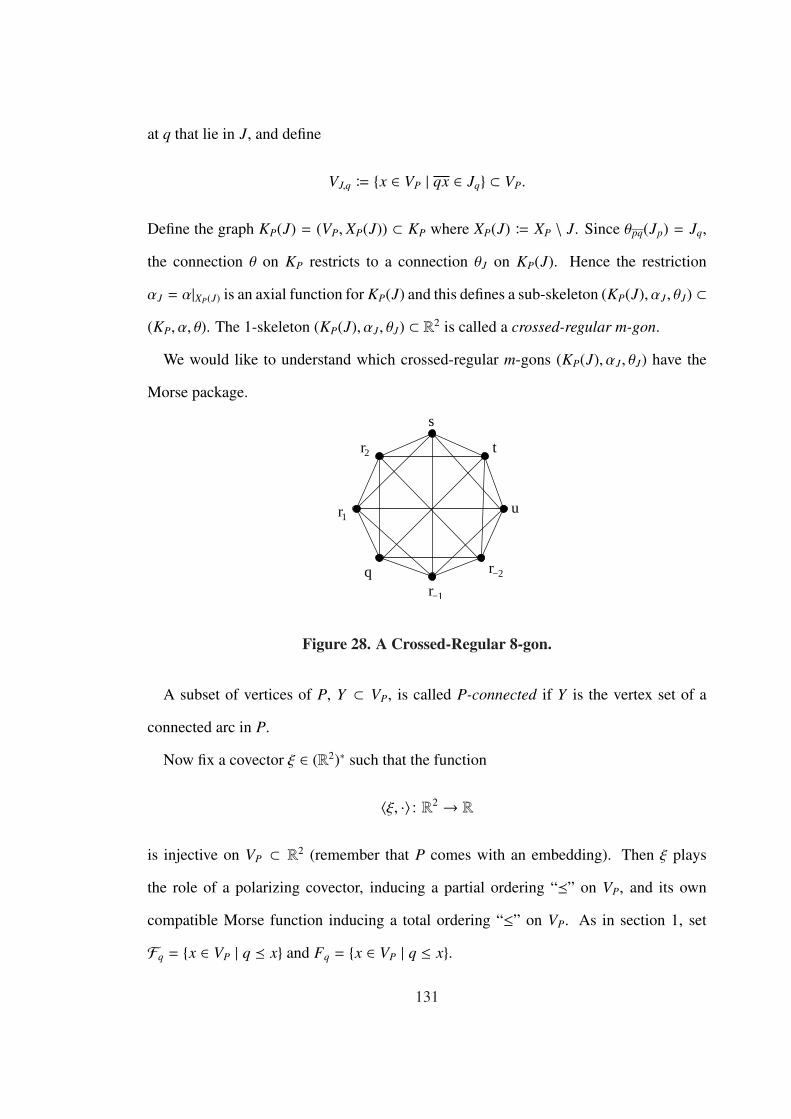
at q that lie in J, and define

VJ,q B {x ∈ VP | qx ∈ Jq} ⊂ VP.

Define the graph KP(J) = (VP, XP(J)) ⊂ KP where XP(J) B XP \ J. Since θpq(Jp) = Jq,

the connection θ on KP restricts to a connection θJ on KP(J). Hence the restriction

αJ = α|XP(J) is an axial function for KP(J) and this defines a sub-skeleton (KP(J), αJ, θJ) ⊂(KP, α, θ). The 1-skeleton (KP(J), αJ, θJ) ⊂ R2 is called a crossed-regular m-gon.

We would like to understand which crossed-regular m-gons (KP(J), αJ, θJ) have the

Morse package.

q

r

r

r

2

1

r−1

−2

s

t

u

Figure 28. A Crossed-Regular 8-gon.

A subset of vertices of P, Y ⊂ VP, is called P-connected if Y is the vertex set of a

connected arc in P.

Now fix a covector ξ ∈ (R2)∗ such that the function

〈ξ, ·〉 : R2 → R

is injective on VP ⊂ R2 (remember that P comes with an embedding). Then ξ plays

the role of a polarizing covector, inducing a partial ordering “�” on VP, and its own

compatible Morse function inducing a total ordering “≤” on VP. As in section 1, set

Fq = {x ∈ VP | q � x} and Fq = {x ∈ VP | q ≤ x}.

131

Lemma 3.2.4. For each vertex q ∈ VP, Fq is P-connected.

Proof. The unique maximum vertex with respect to the total ordering “≤” can be char-

acterized locally as follows: q0 ∈ VP is the unique maximum if and only if q0 is larger

than each of its (two) neighbors (in VP). This is a direct consequence of the convexity of

P.

Let

γ1 : x1 � · · · � xr

γ2 : y1 � · · · � ys

be two P-connected arcs of maximal length in Fq. We will assume that γ1 and γ2 are

distinct and derive a contradiction. If γ1 , γ2, then their vertex sets must be disjoint by

the maximality assumption (if they were not disjoint, we could get a longer P-connected

arc by concatenating γ1 and γ2). Hence the unique maximum vertex in P does not lie in

γ1, say. By the local characterization of the unique maximum, we may assume that γ1 is

ξ-oriented in the sense that xi > xi−1 for 1 ≤ i ≤ r (otherwise there is an 1 ≤ i ≤ r − 1

such that xi+1 < xi > xi−1 which would imply that xi is a the maximum). Let xr+1 ∈ VP

such that xr xr+1 ∈ EP. Now by the maximality of γ1, we must have xr+1 < Fq which

implies that xr+1 < xr. Hence we have xr+1 < xr > xr−1, hence xr is the unique maximum

and lies in γ1, a contradiction. �

For each removal set J, and each vertex q ∈ VP there is a maximal P-connected set

YJ,q ⊂ VP \ VJ,q

that contains q. By the symmetry of P and J, there is a positive integer NJ that is inde-

pendent of q, and a labelling

YJ,q = {r−NJ , r−NJ+1, . . . , r−1, q, r1, . . . , rNJ−1, rNJ }

132

where riri+1 ∈ EP and sq(ri) = r−i for all i, where sq ∈ I(m) denotes the (unique)

non-trivial stabilizer of q. In Figure 28 for example, we have VJ,q = {s, u}, YJ,q =

{r−2, r−1, q, r1, r2}. In this example NJ = 2.

Lemma 3.2.5. If q ∈ VP is any vertex and VJ,q ∩ Fq = ∅ then for any z ∈ Fq we have

VJ,z ∩ Fq = ∅.

Proof. Label

YJ,q = {r−NJ , . . . , r−1, q, r1, . . . , rNJ }

YJ,z = {s−NJ , . . . , s−1, z, s1, . . . , sNJ }

(recall that the symmetry of P and J guarantee that NJ is independent of q). By Lemma

3.2.4 Fq is P-connected. This implies that either Fq = {q} (in which case the state-

ment is vacuous) or that |Fq| ≤ NJ + 1. Indeed if Fq , {q}, then q is not the unique

maximum, hence r−1 and r1 cannot both lie in Fq. Hence Fq ⊂ {q, r1, . . . , rNJ } or

Fq ⊂ {q, r−1, . . . , r−NJ }.Since z ∈ Fq and YJ,z is (by definition) P-connected, we see that Fq ⊂ YJ,z (Fq ∩ YJ,z

must be a P-connected arc of length at most NJ + 1), hence Fq∩VJ,z = ∅. This completes

the proof of Lemma 3.2.5. �

Lemma 3.2.6. Given a removal set J ⊂ XP \ EP, there is a unique vertex qJ ∈ VP

satisfying

i. VJ,qJ∩ FqJ

= ∅

ii. YJ,qJ= {r−NJ , . . . , r−1, qJ, r1, . . . , rNJ } ∩ FqJ

= {qJ, r1, . . . , rNJ }.

Proof. Choose qJ to be the (NJ + 1)st largest vertex with respect to “≤”; that is, choose

qJ so that |FqJ| = NJ + 1. We can label

YJ,qJ= {r−NJ , . . . , r−1, qJ, r1, . . . , rNJ }

133

so that r−1 ≺ qJ ≺ r1. Then r1 ∈ FqJand r−1 < FqJ

. By Lemma 3.2.4 FqJis P-connected,

hence FqJand the P-connected set {qJ, r1, . . . , rNJ } must coincide. This completes the

proof of Lemma 3.2.6. �

ξ

q

r

r

rr

J

1

r23

−3 −2

r−1

Figure 29. The unique vertex qJ

A removal set J is called outer if the set VJ,q is P-connected, for all q ∈ VP. The

resulting 1-skeleton (KP(J), αJ, θJ) is called an outer crossed-regular m-gon. Note that if

J is outer, then VP = YJ,q t VJ,q.

It is straight forward to construct a generating family for the complete regular m-gon

(KP, α, θ). In order to understand the equivariant cohomology ring of (KP(J), αJ, θJ), it

is useful to think of the crossed-regular m-gon as a sub-skeleton of (KP, α, θ). For any

removal set J ⊂ XP \ EP, there is a Thom class τJ ∈ H(KP, α), multiplication by which

gives an inclusion

H(KP(J), αJ)τJ // H(KP, α).

134

Also since (KP(J), αJ, θJ) ⊂ (KP, α, θ) is a sub-skeleton, there is an inclusion morphism

that induces a restriction map on equivariant cohomology rings

H(KP, α) ι∗ // H(KP(J), αJ).

Furthermore since the group I(m) acts on (KP(J), αJ, θJ) via 1-skeleton automorphisms,

there is an induced action of the group I(m) on H(KP(J), αJ); we will denote this action

by g ? f for f ∈ H(KP(J), αJ) and g ∈ I(m).

We have the following result, which is a first step in understanding the Morse package

for crossed-regular polygons.

Theorem 3.2.7. Outer crossed-regular m-gons have the Morse package.

Proof. The idea of the proof is straight forward: view (KP(J), αJ, θJ) as a sub-skeleton

of (KP, α, θ) and use symmetry and the fact that (KP, α, θ) admits a generating family to

construct a generating family for (KP(J), αJ, θJ). Let q ∈ VP be any vertex. We will show

that q admits a pseudo-generating class. There are three cases to consider.

i. 〈ξ, α(e)〉 > 0 for each e ∈ Jq: In this case we let τq be the generating class for q

in H(KP, α). Then its restriction ι∗τq ∈ H(KP(J), αJ) is a pseudo-generating class:

supp(ι∗τq) ⊂ Fq and

ι∗τq(q) =∏

e∈X(J)−q

α(e).

See Figure 31.

ii. 〈ξ, α(e)〉 < 0 for each e ∈ Jq: In this case we let τq be the generating class for q

in H(KP, α). Note that the support of τq is contained in Fq and that in this case

VJ,q ∩ Fq = ∅. Hence by Lemma 3.2.5, VJ,z ∩ Fq = ∅ for each z ∈ Fq. Hence

τq(z) = Kz ·∏

e∈Jz

α(e) (3.2.9)

135

for some Kz ∈ S depending on z ∈ Fq. The claim now is that the function

τq : X(J)→ S defined by

τq(z) =

Kz if z ∈ Fq

0 otherwise

is actually an equivariant class on (KP(J), αJ). The point is that for zz′ ∈ X(J) we

have

τq(z) − τq(z′) ≡ 0 mod α(zz′)

and∏

e∈Jz

α(e) −∏

e′∈Jz′

α(e′) ≡ 0 mod α(zz′).

Since∏

e∈Jzα(e) . 0 mod α(zz′) we must have that

Kz − Kz′ ≡ 0 mod α(zz′)

as well. Thus τq is an equivariant class. Clearly supp(τq) ⊂ Fq. Finally note that

Kq =∏

e∈X(J)qαJ(e) by (3.2.9), since τq is a generating class for q (in (KP, α)); thus

τq is a generating class for q on (KP(J), αJ). See Figure 31.

iii. 〈ξ, α(e1)〉 > 0 > 〈ξ, α(e2)〉 for some e1, e2 ∈ Jq: In this case we appeal to the

symmetry of (KP(J), αJ, θJ) and Lemma 3.2.6. Let qJ ∈ VP be the unique vertex

as in Lemma 3.2.6. By symmetry there exists a group element g ∈ I(m) such

that g(qJ) = q. Since I(m) is acting by graph morphisms (in fact, I(m) acts by

1-skeleton morphisms), g takes the P-connected subset

FqJ⊂ YJ,qJ

⊂ VP \ VJ,qJ

to a P-connected subset

g(FqJ) ⊂ YJ,q ⊂ VP \ VJ,q.

136

By Lemma 3.2.6, |g(FqJ)| = |FqJ

| = NJ +1. Since in this case we have VJ,q∩Fq , ∅,we must have |Fq| > NJ +1. The claim is that we may assume that the P-connected

set g(FqJ) lies in Fq. To see this write the sets

YJ,qJ= {r−NJ , . . . , r−1, qJ, r1, . . . , rNJ }

and

YJ,q = {s−NJ , . . . , s−1, q, s1, . . . , sNJ }.

By Lemma 3.2.6 we have that

YJ,qJ∩ FqJ

= {qJ, r1, . . . , rNJ }.

Thus since g(qJ) = q, the set g(FqJ) ∩ YJ,q must be a P connected arc lying on one

side of q or the other; by reflecting about q, we may assume that g(FqJ) ∩ YJ,q =

{q, s1, . . . , sNJ } ⊂ Fq.

Hence g(qJ) = q and g(FqJ) ⊂ Fq. By case 2, there is a class τqJ

∈ H(KP(J), αJ)

whose support lies in FqJand whose value at qJ is

τqJ(qJ) =

∏

e∈X(J)−qJ

α(e).

Set τq = g ? τqJ. Then

supp(τq) ⊂ g(FqJ) ⊂ Fq

and

τq(q) =∏

e∈X(J)−qJ

g (α(e)) =∏

e∈X(J)−q

α(e);

to see the second equality, note that X(J)−qJ=

{qJ x | x ∈ YJ,qJ

\ FqJ

}. Since g(FqJ

) ⊂Fq and g(YJ,qJ

) = YJ,q, it follows that g(YJ,qJ\FqJ

) = YJ,q\Fq, hence that g(X(J)−qJ) =

X(J)−q . Thus τq is a pseudo-generating class for q. See Figure 31

137

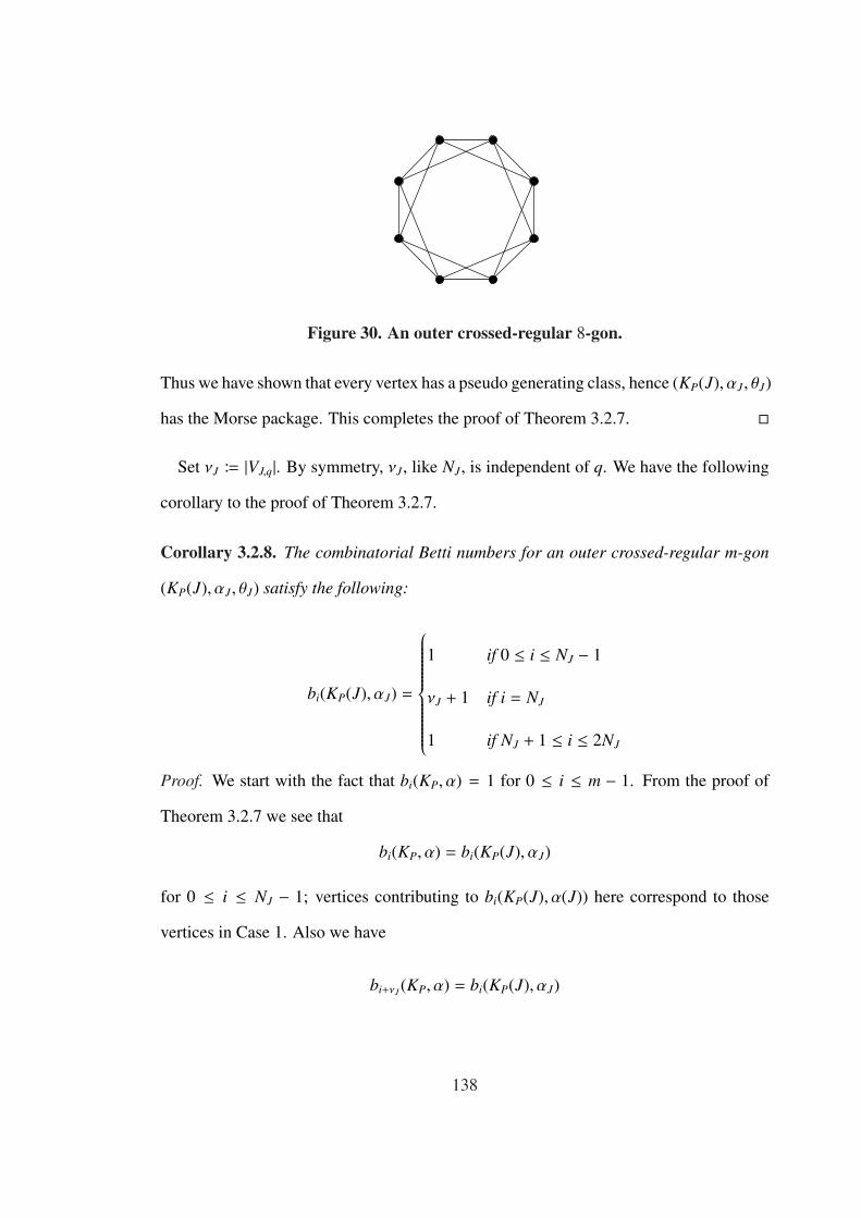
Figure 30. An outer crossed-regular 8-gon.

Thus we have shown that every vertex has a pseudo generating class, hence (KP(J), αJ, θJ)

has the Morse package. This completes the proof of Theorem 3.2.7. �

Set νJ B |VJ,q|. By symmetry, νJ, like NJ, is independent of q. We have the following

corollary to the proof of Theorem 3.2.7.

Corollary 3.2.8. The combinatorial Betti numbers for an outer crossed-regular m-gon

(KP(J), αJ, θJ) satisfy the following:

bi(KP(J), αJ) =

1 if 0 ≤ i ≤ NJ − 1

νJ + 1 if i = NJ

1 if NJ + 1 ≤ i ≤ 2NJ

Proof. We start with the fact that bi(KP, α) = 1 for 0 ≤ i ≤ m − 1. From the proof of

Theorem 3.2.7 we see that

bi(KP, α) = bi(KP(J), αJ)

for 0 ≤ i ≤ NJ − 1; vertices contributing to bi(KP(J), α(J)) here correspond to those

vertices in Case 1. Also we have

bi+νJ (KP, α) = bi(KP(J), αJ)

138

ξ

ξ

ξ

Case 3

Case 2

Case 1

Figure 31. The 3 cases

for NJ + 1 ≤ i ≤ 2NJ; vertices contributing to bi(KP(J), α(J)) here correspond to those

vertices in Case 2. Finally the middle Betti number

bNJ (KP(J), αJ) = m − 2NJ = (2NJ + 1 + νJ) − 2NJ = νJ + 1.

This completes the proof of Corollary 3.2.8. �

Crossed-regular polygons provide a large source of interesting examples of straight

planar 1-skeleta (they are GKM). Many of them have the Morse package, but some do

not. For example, the 4-valent crossed-regular 7-gon shown in Figure 32 does not have

the Morse package.

139

?

?

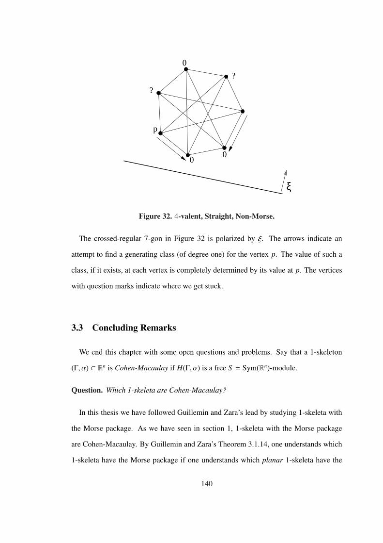
0

p

ξ

00

Figure 32. 4-valent, Straight, Non-Morse.

The crossed-regular 7-gon in Figure 32 is polarized by ξ. The arrows indicate an

attempt to find a generating class (of degree one) for the vertex p. The value of such a

class, if it exists, at each vertex is completely determined by its value at p. The vertices

with question marks indicate where we get stuck.


We end this chapter with some open questions and problems. Say that a 1-skeleton

(Γ, α) ⊂ Rn is Cohen-Macaulay if H(Γ, α) is a free S = Sym(Rn)-module.

Question. Which 1-skeleta are Cohen-Macaulay?

In this thesis we have followed Guillemin and Zara’s lead by studying 1-skeleta with

the Morse package. As we have seen in section 1, 1-skeleta with the Morse package

are Cohen-Macaulay. By Guillemin and Zara’s Theorem 3.1.14, one understands which

1-skeleta have the Morse package if one understands which planar 1-skeleta have the

140

Morse package.

Question. Which planar 1-skeleta have the Morse package?

We showed in Section 2 that our straight-ness condition is equivalent to the Morse

package in the 3-valent case. However the 1-skeleton shown in Figure 32 shows that

straight-ness is not a sufficient condition for the Morse package, even in the 4-valent

case.

Problem. Classify planar k-valent 1-skeleta with the Morse package for k ≥ 4.

It may be enlightening (and easier) to first deal with the crossed-regular polygon case.

Problem. Classify crossed-regular polygons that have the Morse package.

141

C H A P T E R 4

STRONG LEFSCHETZ PROPERTIES

We continue our study of the cohomology rings associated to a 1-skeleton. In this

chapter we study the strong Lefschetz properties of the ordinary cohomology ring of a

1-skeleton. In contrast to the previous chapter, in this chapter we are interested in the

multiplicative structure of the ordinary cohomology ring. We will however find it useful

to refer back to the equivariant cohomology ring, especially when we discuss various

decomposition theorems.

The study of the strong Lefschetz property for rings in general is motivated largely by

the hard Lefschetz theorem in algebraic geometry. In certain cases when a 1-skeleton

comes from a GKM T -manifold, we can appeal to the hard Lefschetz theorem to deduce

that its cohomology ring has the strong Lefschetz property. One would like to find an

alternative proof of this fact that does not appeal to the hard Lefschetz theorem. Such an

alternative proof would (hopefully) have the added benefit of extending such results to a

class of 1-skeleta beyond those coming from GKM T -manifolds.

We give a couple of results in this direction in the way of “Lefschetz consructions”.

By a construction on 1-skeleta, we mean some operation that takes two 1-skeleta and

somehow produces a new 1-skeleta; the product and blow-up construction of Chapter 2

are examples and we introduce another one here called the fiber bundle, due to Guillemin,

Sabatini, and Zara. The two main results of this chapter are algebraic in nature. One

142

implies that if the base and the fiber of a fiber bundle have the Lefschetz package, then

the total space also has the Lefschetz package. The other implies that if a 1-skeleton

and a (level) sub-skeleton both have the Lefschetz package, then the blow-up of the

1-skeleton along the sub-skeleton also has the Lefschetz package. As an application,

one can apply the fiber bundle ideas to the theory of finite reflection groups and their

coinvariant rings; the result is a new conceptual proof (applicable in most types) of the

fact that the coinvariant ring of a finite reflection group has the strong Lefschetz property.

This chapter is divided into five sections. In Section 1, we give the preliminary defini-

tions, and attempt to give some motivation for studying rings with the strong Lefschetz

property. In Section 2 we define the notion of a fiber bundle of 1-skeleta and state a de-

composition result of Guillemin, Sabatini, and Zara. We then state and prove one of our

main algebraic results; this will imply that the fiber bundle is a Lefschetz construction.

In Section 3 we briefly review the blow-up construction (from Chapter 2) and prove a

decomposition result for the cohomology ring of the blow-up due to Guillemin and Zara.

We then state and prove our other main algebraic result; this will imply that the blow-up

is a Lefschetz construction. In Section 4 we give some of the basic facts in the theory

of root systems and finite reflection groups and their coinvariant rings. We then show

how to construct a 1-skeleton from a root system and its finite reflection group and give

a map explicitly relating the coinvariant ring of the finite reflection group to the coho-

mology ring of the associated 1-skeleton. We then proceed (using the language of finite

reflection groups and coinvariant rings) to use the fiber bundle ideas above to show that

the coinvariant ring has the strong Lefschetz property (for most finite reflection groups).

In Section 5 we give a few concluding remarks.

143

4.1 Preliminaries and Motivation

Let R be an N-graded Artinian R algebra; that is

R =⊕

i∈NRi

is a graded ring with R0 = R and Ri = 0 for all i > d for some d < ∞. We can therefore

write

R =

d⊕

i=0

Ri

where d = max{i ∈ N | Ri , 0}. We say that R is symmetric if dimR Ri = dimR Rd−i for

each i. Given an element l ∈ R1, multiplication defines linear maps

Ri l // Ri+1

x // lx.

We say that l ∈ R1 is a strong Lefschetz element if the maps

ld−2i : Ri → Rd−i

are isomorphisms for 0 ≤ i ≤ b d2c. A very simple, but fundamental example is the ring

R[Y]/〈Yn〉 for n ≥ 0 (with the usual grading). Here a strong Lefschetz element is given

by Y ∈ (R[Y]/〈Yn〉)1.

Let (Γ, α) ⊂ Rn be a d-valent 1-skeleton with equivariant cohomology ring H(Γ, α)

and ordinary cohomology ring H(Γ, α) and let S ↪→ H(Γ, α) denote the polynomial ring

on (Rn)∗ included as the constant functions on VΓ.

H(Γ, α) is an N-graded Artinian R-algebra. Indeed, H(Γ, α) is an N-graded R-algebra

since it is the quotient of an N-graded S -algebra by the ideal generated by the unique

homogeneous maximal ideal S + ⊂ S . Furthermore it is finitely generated since it is the

quotient of a finitely generated S -module.

144

We are interested in finding conditions on a 1-skeleton (Γ, α) ⊂ Rn that guarantee the

cohomology ring H(Γ, α) has the strong Lefschetz property. We will say that a 1-skeleton

has the Lefschetz package if its cohomology ring has the strong Lefschetz property.

The study of the strong Lefschetz property of graded rings is rooted in the study of the

topology of algebraic varieties. A deep theorem in algebraic geometry implies that the

cohomology rings of certain algebraic varieties have the strong Lefschetz property. The

theorem is named in honor of Solomon Lefschetz and is aptly called “the hard Lefschetz

theorem”.

Theorem 4.1.1. (hard Lefschetz) Let X be a smooth projective algebraic variety over C

and let H(X;R) denote the (topological) cohomology ring of X with coefficients in R. Let

ω ∈ H2(X;R) denote the cohomology class of a smooth hyperplane section. Let

LX : Hi(X;R)→ Hi+2(X;R)

denote the linear map “cup-product with ω”. Then for 0 ≤ i ≤ d, where dim(X) = d the

map

Ld−iX : Hi(X;R)→ H2d−i(X;R)

is an isomorphism.

For more details on this theorem and its history see Messing’s article [23]. Theorem

4.1.1 can be used to show that certain 1-skeleta have the strong Lefschetz package. For

example suppose that X is a smooth projective toric variety of dim(X) = d (in particular

X is a GKM T -manifold). Then X is uniquely determined by a simplicial fan ∆(X) ⊂(Rd)∗ and if we fix an embedding X ↪→ PN , this uniquely determines a d-polytope P ⊂ Rd

whose inner normal fan is ∆(X). Let (ΓP, αP) ⊂ Rd be the d-valent 1-skeleton of the

simple d-polytope P. One can show that the cohomology ring H(X;R) is isomorphic to

145

the cohomology ring H(ΓP, αP) via a natural degree-halving map:

H2∗(X;R) � // H∗(ΓP, αP).

Letω ∈ H2(X;R) be the cohomology class of a smooth hyperplane section as in Theorem

4.1.1 and let l ∈ H1(ΓP, αP) be the corresponding class on (ΓP, αP). Since the cohomol-

ogy of X vanishes in odd degree we can rewrite the statement of Theorem 4.1.1 as the

map

Ld−2iX : H2i(X;R)→ H2d−2i(X;R)

is an isomorphism for 0 ≤ i ≤ b d2c.

Then we have the commutative diagram

H2i(X;R)

Ld−2iX

²²

� // Hi(ΓP, αP)

ld−2i

²²

H2d−2i(X;R) �// Hd−i(ΓP, αP);

this shows that (ΓP, αP) has the strong Lefschetz package. For more details on the corre-

spondence between toric varieities and polytopes, see [9].

More generally if M is a GKM T -manifold that has the structure of a projective variety

over C for which the T action is linear algebraic, then M will be equivariantly formal in

the sense of Goresky, Kottwitz and MacPherson, hence, by a theorem in [10] (Theorem

7.2, page 44) H2∗(M;R) � H∗(Γ, α). In this case we can also apply Theorem 4.1.1 to

deduce that (Γ, α) has the Lefschetz package.

The above argument for toric varieties is essentially the one used by Stanley in [26] to

prove the “necessity” direction of McMullen’s celebrated g-conjecture (g-theorem now)

on the face numbers of simple polytopes. An important point is that the 1-skeleton of a

GKM T -manifold is necessarily integral, meaning that the axial function takes values in

some integral lattice. In order to deduce the result for all simple polytopes, Stanley had

to give some deformation arguments, since all simple polytopes are not integral a priori.

146

See [26] for more details. Later McMullen gave a different proof of the same result in

[22]. Essentially McMullen showed that the 1-skeleton (ΓP, αP) of a simple d-polytope

P has the strong Lefschetz package without appealing the Theorem 4.1.1, although the

language he used differs from ours here (for instance there is no mention of “1-skeleta” or

“cohomology rings” in his work). Timorin later gave a simplified version of McMullen’s

proof in his paper [27]. One nice feature about McMullen’s argument is that it holds for

all simple polytopes, integral or not. In particular McMullen’s result holds for simple

polytopes that do not come from any T -space. This can be considered the starting point

of the investigations in this chapter. To what extent does the strong Lefschetz property

hold for more general 1-skeleta, rational or not? One approach that has been fruitful is

finding so-called Lefschetz constructions on 1-skeleta.

4.2 Fiber Bundles

In this section we introduce the general notion of a fiber-bundle over a 1-skeleton.

Guillemin, Sabatini and Zara introduced and studied the notions of fibrations and fiber

bundles of (GKM) 1-skeleta in [28]; the definitions here are, for the most part, due to

them. We will try to follow their notation. We will however drop the “GKM” assumption.

First we recall the definition of a morphism of 1-skeleta with connections. Let (Γ, α, θ) ⊂Rn and (Γ′, α′, θ′) ⊂ Rm be 1-skeleta with connections.

Definition 4.2.1. A morphism of 1-skeleta with connections is a pair

π = (πG, πL) : (Γ, α, θ)→ (Γ′, α′, θ′)

where

i. πG : VΓ t EΓ → VΓ′ t EΓ′ is a morphism of graphs (“G” for “graph”)

147

ii. πL : (Rn)∗ → (Rm)∗ is a linear map (“L” for “linear”) making the following dia-

gram commute:

Rm (πL)∗// Rn

EΓ′

α′

OO

π−1G (E′

Γ) B Eh

Γ,

α

OO

πGoo

iii. θ sends horizontal edges to horizontal edges (i.e. θpq((EhΓ)p) ⊆ (Eh

Γ)q for all pq ∈

EΓ) and along horizontal edges pq ∈ EhΓ

the following diagram commutes:

(EhΓ)p

πG //

θpq

²²

(EΓ′)πG(p)

θ′πG (pq)

²²

(EhΓ)q πG

// (EΓ′)πG(q).

We say that π is an isomorphism (of 1-skeleta with connections) if the maps πG and πL

are both bijective. In this case there is a uniquely determined morphism

π = (πG, πL) : (Γ′, α′, θ′)→ (Γ, α, θ)

where πG = π−1G and πL = π−1

L . The morphism π is called the inverse of π and we write

π = π−1.

Given a totally geodesic sub-skeleton (Γ′0, α′0, θ′0) ⊂ (Γ′, α′, θ′) we can look at the pre-

image of the graph Γ′0 under πG; that is the sub-graph π−1G (Γ′0) ⊂ Γ. Without any further

restrictions on the morphism π, this sub-graph need not be the graph of a totally geodesic

sub-skeleton.

Definition 4.2.2. A morphism of 1-skeleta with connections

π = (πG, πL) : (Γ, α, θ)→ (Γ′, α′, θ′)

is called a fibration of 1-skeleta with connections if

148

i. πG : (EhΓ)p → (EΓ′)πG(p) is bijective for every p ∈ VΓ

ii. Rm = Rn and πL is the identity map.

iii. For vertical edges pq ∈ EvΓ

where πG(p) = r = πG(q), the map θpq : (EhΓ)p → (Eh

Γ)q

makes the following diagram commutes:

(EhΓ)p

πG

�((QQQQQQQQQQQQQQ

θpq

²²

(EΓ′)r.

(EΓ)q

πG

�66mmmmmmmmmmmmmm

As the name suggests, the conditions on a fibration are sufficient to ensure that the

pre-image of a sub-skeleton is a sub-skeleton. We state this as a theorem.

Theorem 4.2.3. Let π : (Γ, α, θ) → (Γ′, α′, θ′) be a fibration of 1-skeleta with connec-

tions. Let (Γ′0, α′0, θ′0) ⊂ (Γ′, α′, θ′) be a totally geodesic sub-skeleton. Then the pre-image

sub-graph

Γ0 B π−1G (Γ′0) ⊂ Γ

has constant valency and is the graph of a totally geodesic sub-skeleton (Γ0, α0, θ0) ⊂(Γ, α, θ).

Proof. Set Γ0 = (V0, E0). We want to show that |(E0)p| is independent of the vertex

p ∈ V0.

For all vertices r ∈ VΓ we have (EΓ)r = (EhΓ)r t (Ev

Γ)r and, if we set r′ B πG(r), then by

condition (i) in Definition 4.2.2 the map πG : (EhΓ)r → (EΓ′)r′ is bijective. For r′ ∈ VΓ′0 ,

set (Eh0)r B (πG|r)−1((EΓ′0)r′). Then for all vertices r ∈ VΓ0 we have

(E0)r = (Eh0)r t (Ev

Γ)r. (4.2.1)

149

Now

|(Eh0)r| = (valency of Γ′0) (4.2.2)

and

|(EvΓ)r| = (valency of Γ) − (valency of Γ′). (4.2.3)

Combining (4.2.2) and (4.2.3) with (4.2.1), we see that Γ0 must have constant valency.

Now we want to show that the connection θ on Γ restricts to give a connection θ0 on

Γ0. Let pq ∈ E0 be any edge in Γ0. We need to show that

θpq((E0)p) = (E0)q. (4.2.4)

By condition (iii) of Definition 4.2.1 we have that

θpq((EhΓ)p) ⊂ (Eh

Γ)q.

Since θpq : (EΓ)p → (EΓ)q is bijective and |(EhΓ)p| = |(Eh

Γ)q| we must in fact have

θpq((EhΓ)p) = (Eh

Γ)q,

and hence we must also have

θpq((EvΓ)p) = (Ev

Γ)q (4.2.5)

for all pq ∈ EΓ0 .

By (iii) in Definition 4.2.1, we have the commutative diagram

(Eh0)p

πG //

θpq

²²

(EΓ′0)πG(p)

θ′πG (pq)

²²

(Eh0)q πG

// (EΓ′0)πG(q)

for pq ∈ EhΓ. Thus θpq((Eh

0)p) = (Eh0)q for all pq ∈ Eh

0. For pq ∈ EvΓ

we must also have

θpq((Eh0)p) = (Eh

0)q (4.2.6)

by condition (iii) in Definition 4.2.2. Combining (4.2.5) and (4.2.6) with (4.2.1) yields

(4.2.4), as desired. �

150

Theorem 4.2.3 shows that in particular, the fibers π−1G (p′) B Γp′ ⊂ Γ are totally

geodesic. For each p′ ∈ VΓ′ let (Γp′ , αp′ , θp′) ⊂ (Γ, α, θ) denote the sub-skeleton on

the graph π−1G (p′) ⊂ Γ; for short we write π−1(p′) ⊂ (Γ, α, θ).

Figure 33. a fibration

Figure 33 shows a fibration over a single edge; its fibers are the quadralaterals shown

on either end.

Now we impose further restrictions (following Guillemin, Sabatini and Zara) that al-

low us to “transport” fibers along paths in the base. This brings us to the notion of a fiber

bundle of 1-skeleta.

Definition 4.2.4. A morphism π : (Γ, α, θ)→ (Γ′, α′, θ′) is a fiber bundle of 1-skeleta with

connections (over (Γ′, α′, θ′)) if

i. π is a fibration

ii. for every edge e′ B p′q′ ∈ EΓ′ there are isomorphisms of 1-skeleta with connec-

tions

Ψe′ = ((Ψe′)G, (Ψe′)L) : π−1(p′)→ π−1(q′)

151

such that for each vertex p ∈ π−1G (p′) ∩ VΓ, if q = (Ψe′)G(p) ∈ π−1

G (q′) then pq ∈(Eh

Γ)p.

The isomorphisms {Ψe′}e′∈EΓ′ are called transition morphisms of the fiber bundle π.

For each p′ ∈ VΓ′ let

ip′ : π−1(p′) ↪→ (Γ, α, θ)

denote the natural inclusion morphism. We will express a fiber bundle of 1-skeleta in the

“traditional” notation:

π−1(p′)ip′

// (Γ, α, θ)

π

²²

(Γ′, α′, θ′).

Here π−1(p′) is called the fiber over p′, (Γ, α, θ) is called the total space and (Γ′, α′, θ′)

is called the base of the fiber bundle π.

Remark. Definitions 4.2.2 and 4.2.4 are due for the most part to Guillemin, Sabatini

and Zara. We say “for the most part” here because in [28], they work only with GKM

1-skeleta. Also condition (iii) in Definition 4.2.2 is not mentioned in [28]. However it

is not difficult to see that given a fibration of 1-skeleta with connections π : (Γ, α, θ) →(Γ′, α′, θ′) in the sense of Definition 4.2.2 (i) and (ii) (without assuming condition (iii)),

there is always a (possibly different) connection θ to be found on (Γ, α) so that π : (Γ, α, θ)→(Γ′, α′, θ′) is a fibration of 1-skeleta with connections in the sense of Definition 4.2.2 (i),

(ii), and (iii).

What we call a fibration of 1-skeleta with connections is called a GKM-fibration and

what we call a fiber bundle of 1-skeleta with connections, is called a GKM-fiber bundle

in [28].

Figure 34 shows a typical fiber bundle of 1-skeleta; the linear part of the transition

map across a horizontal edge in this case is reflection about the line perpendicular to that

152

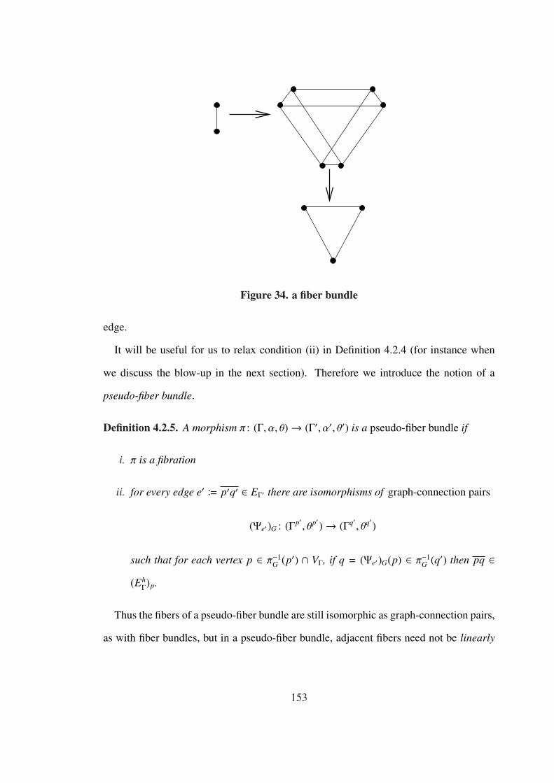
Figure 34. a fiber bundle

edge.

It will be useful for us to relax condition (ii) in Definition 4.2.4 (for instance when

we discuss the blow-up in the next section). Therefore we introduce the notion of a

pseudo-fiber bundle.

Definition 4.2.5. A morphism π : (Γ, α, θ)→ (Γ′, α′, θ′) is a pseudo-fiber bundle if

i. π is a fibration

ii. for every edge e′ B p′q′ ∈ EΓ′ there are isomorphisms of graph-connection pairs

(Ψe′)G : (Γp′ , θp′)→ (Γq′ , θq′)

such that for each vertex p ∈ π−1G (p′) ∩ VΓ, if q = (Ψe′)G(p) ∈ π−1

G (q′) then pq ∈(Eh

Γ)p.

Thus the fibers of a pseudo-fiber bundle are still isomorphic as graph-connection pairs,

as with fiber bundles, but in a pseudo-fiber bundle, adjacent fibers need not be linearly

153

related. We will use the same notation to denote a pseudo-fiber bundle:

π−1(p′)ip′

// (Γ, α, θ)

π

²²

(Γ′, α′, θ′).

Shown in Figure 35 is an example of a pseudo-fiber bundle (over a single edge, with

fibers complete 1-skeleta on 4-vertices) that fails to be a fiber bundle in the sense of

Definition 4.2.4. This pseudo-fiber bundle actually arises as a GKM T -manifold: the

total space is a 3 dimensional toric variety, X, over C with a dense open torus T = (C∗)3,

and T ⊂ T is a codimension one sub-torus acting on X by restriction.

Figure 35. a pseudo-fiber bundle

Note that the fibration of 1-skeleta (with connections) shown in Figure 33 is not even

a pseudo-fiber bundle, let alone a fiber bundle of 1-skeleta (with connections).

154

Special Cases

We take this opportunity to point out some relavent special cases of fiber bundles and

pseudo-fiber bundles.

Direct Product

Let (Γ′, α′, θ′), (Γ0, α0, θ0) ⊂ Rn be two 1-skeleta with connections in Rn. We construct

the direct product 1-skeleton (Γ, α, θ) ⊂ Rn as follows: Set Γ = (VΓ, EΓ) where

VΓ = VΓ0 × VΓ′

and

EΓ = EΓ0 × VΓ′ t VΓ0 × EΓ′;

we shall set

EhΓ = VΓ0 × EΓ′

and

EvΓ = EΓ0 × VΓ′ .

We have natural projection morphisms of graphs

(π′)G : Γ→ Γ′

and

(π0)G : Γ→ Γ0.

Define the function

α : EΓ → Rn

by

α(e) =

α′((π′)G(e)) if e ∈ EhΓ

α0((π0)G(e)) if e ∈ EvΓ.

155

Define θ to be the unique connection on Γ whose restriction to

{v0} × Γ′

is θ′ for each v0 ∈ VΓ0 and on

Γ0 × {v′}

is θ0 for each v′ ∈ VΓ′ . This defines a 1-skeleton (Γ, α, θ) ⊂ Rn called the direct product

1-skeleton with factors (Γ0, α0, θ0) and (Γ′, α′, θ′). As indicated above we will regard

(Γ′, α′, θ′) as the “horizontal” factor and (Γ0, α0, θ0) as the “vertical” factor. Then as one

might expect, the projection morphism

π′ = ((π′)G, IRn) : (Γ, α, θ)→ (Γ′, α′, θ′)

is a fiber bundle of 1-skeleta; the map π′G : (EhΓ)p → (EΓ′)π′G(p) is a bijection for each

vertex p ∈ VΓ and fibers are just (π′G)−1(p′) = Γ0 × {p′}. The transition morphisms

Ψe′ = ((Ψe′)G, (Ψe′)L) : π−1(p′)→ π−1(q′)

are trivial with

(Ψe′)G : Γ0 × {p′} → Γ0 × {q′}

defined by

(Ψe′)G(x, p′) = (x, q′)

and

(Ψe′)L = IRn : Rn → Rn.

Remark. Note that we could have set (Γ0, α0, θ0) to be the “horizontal” factor and

(Γ′, α′, θ′) the “vertical” factor. In that case the projection morphism

(π0) = ((π0)G, IRn) : (Γ, α, θ)→ (Γ0, α0, θ0)

is also a fiber bundle of 1-skeleta with connections with general fiber (Γ′, α′, θ′).

156

Blow-Up

Let (Γ, α, θ) ⊂ Rn be a 1-skeleton and let (Γ0, α0, θ0) ⊂ (Γ, α, θ) be a level sub-skeleton.

We have seen in chapter 2 that we can construct a new 1-skeleton (Γ], α], θ]) ⊂ Rn called

the blow-up of (Γ, α, θ) along (Γ0, α0, θ0). The blow-up comes equipped with a morphism

of 1-skeleta with connections

β = (βG, IRn) : (Γ], α], θ])→ (Γ, α, θ)

called the blow-down morphism. Let

β−1(Γ0, α0, θ0) ⊂ (Γ], α], θ])

denote the singular locus of the blow-up; by Theorem 4.2.3 it is a totally geodesic sub-

skeleton that we denote by

(Γ]0, α]0, θ

]0).

Then the restriction of the blow-down to the singular locus is a pseudo-fiber bundle

over the sub-skeleton (Γ0, α0, θ0). That is, the morphism

β0 : (Γ]0, α]0, θ

]0)→ (Γ0, α0, θ0)

is a fibration of 1-skeleta with connections whose fibers are complete 1-skeleta (1-skeleta

whose underlying graph is a complete graph), and the transition maps for e0 B p0q0 ∈EΓ0 ,

(Ψe0)G : (Γp0 , θp0)→ (Γq0 , θq0)

arise naturally from the normal connection maps

θ⊥e0: N0

p0→ N0

q0.

While the blow-down morphism may be a fiber bundle of 1-skeleta in some cases, it

will only be a pseudo-fiber bundle in general. For a more detailed description of this

157

construction, the reader is directed to the discussion in chapter 2. We will have more to

say about the cohomology rings of the blow-up in the next section.

4.2.1 Leray-Hirsch Theorem

A (pseudo-) fiber bundle of 1-skeleta with connections gives a precise way to “de-

compose” certain 1-skeleta with connections into smaller “pieces” called the base and

the fiber (although technically the base does not constitute a sub-skeleta). As one might

hope, under certain additional hypotheses, this geometric decomposition leads to an al-

gebraic decomposition of the ordinary cohomology ring of the total space in terms of the

cohomology rings of the base and the fiber. There is an anlogue of the Leray-Hirsch de-

composition on (topological) cohomology rings for fiber bundles (of topological spaces)

in the 1-skeleton setting, due to Guillemin, Sabatini and Zara.

While we are interested in studying the ordinary cohomology rings, the equivariant

cohomology has a much more concrete, geometric description that is easier to use in

general. The strategy to prove this Leray-Hirsch decomposition for the ordinary coho-

mology is to first derive an “equivariant version” of the decomposition for the equivariant

cohomology rings of a fiber bundle. Then once the result is established for equivariant

cohomology, the result for ordinary cohomology will follow from purely formal consid-

erations.

Given 1-skeleta (Γ, α) ⊂ Rn and (Γ′, α′) ⊂ Rm and a morphism π : (Γ, α) → (Γ′, α′),

the induced map π∗ : H(Γ′, α′)→ H(Γ, α) endows H(Γ, α) with the structure of a module

over H(Γ′, α′). If π is a (pseudo-) fiber bundle this module structure is very well behaved

under certain additional hypotheses. The following result of Guillemin, Sabatini and

Zara is an analogue of the Leray-Hirsch theorem for fiber bundles in algebraic topology.

We refer the reader to [28] for the proof.

158

Theorem 4.2.6. ([28]) Let

π−1(p′)ip′

// (Γ, α, θ)

π

²²

(Γ′, α′, θ′)

be a (pseudo-) fiber bundle of 1-skeleta with connections. Assume that

1. H(π−1(p′)) is a free S -module for all p′ ∈ VΓ′ and

2. there exist classes c1, . . . , cN ∈ H(Γ, α) such that the restrictions i∗p′(c1), . . . , i∗p′(cN) ∈H(π−1(p′)) are an S -basis for all p′ ∈ VΓ′ .

Then the classes c1, . . . , cN are a free H(Γ′, α′)-module basis for H(Γ, α).

Equivalently for any p′ ∈ VΓ′ the map

H(π−1(p′)) ⊗S H(Γ′, α′) Φ // H(Γ, α)

i∗p′(ci) ⊗ f // ci · π∗( f ).

is an isomorphism of H(Γ′, α′)-modules (where the module structure on the tensor prod-

uct is multiplication in the first factor).

Proof. See [28], Theorem 3.6. �

Although we do not need it in the sequel, the following seems to be a useful fact in

the theory of (GKM) fiber bundles.

In the case where

π−1(p′)ip′

// (Γ, α, θ)

π

²²

(Γ′, α′, θ′)

is a GKM-fiber bundle of 1-skeleta with connections (i.e. a fiber bundle whose base,

fiber and total space are all GKM 1-skeleta), the following lemma tells us that to check

159

if classes c1, . . . , cN ∈ H(Γ, α) actually restrict to an S -basis on every fiber, it is enough

to check that they do so on a single fiber.

Lemma 4.2.7. Let

π−1(p′)ip′

// (Γ, α, θ)

π

²²

(Γ′, α′, θ′)

be a GKM-fiber bundle (i.e. a fiber bundle of GKM 1-skeleta with connections). Assume

that H(π−1(p′)) is a free S -module. Suppose that c1, . . . , cN ∈ H(Γ, α) are classes such

that

i∗p′(c1), . . . , i∗p′(cN) ∈ H(Γ0, α0)

are an S -basis for some p′ ∈ VΓ′ . Then

i∗q′(c1), . . . , i∗q′(cN) ∈ H(Γ0, α0)

are an S -basis for all q′ ∈ VΓ′ .

Before we prove Lemma 4.2.7 we need a sub-lemma describing the linear part of the

transition morphisms. This is due to Guillemin, Sabatini, and Zara.

Sub-Lemma 1. Given a GKM-fiber bundle

π−1(p′)ip′

// (Γ, α, θ)

π

²²

(Γ′, α′, θ′),

an oriented edge e′ B p′q′ ∈ EΓ′ we can choose a transition morphism Ψe′ : π−1(p′) →π−1(q′), such that

(Ψe′)L(x) = x + c(x)α′(e′)

for all x ∈ Rn and some linear functional c : Rn → R.

160

Proof. See [28] Proposition 2.11. �

Now we are ready to prove Lemma 4.2.7.

Proof of Lemma 4.2.7. Let c1, . . . , cN ∈ H(Γ, α) be classes such that

i∗p′(c1), . . . , i∗p′(cN) ∈ H(Γ0, α0)

are a basis. To prove Lemma 4.2.7, it suffices to show that

i∗q′(c1), . . . , i∗q′(cN) ∈ H(Γ0, α0)

is a basis for e′ B p′q′ ∈ EΓ′ . Let Ψe′ denote the transition morphism.

We have the following (non-commutative in general) diagram:

π−1(p′)ip′

))RRRRRRRRRRRRRR

(Γ, α, θ)

π−1(q′).

Ψe′

OO

iq′

55llllllllllllll

Since the classes

{i∗p′(ci)}Ni=1 ⊂ H(π−1(p′))

are an S -module basis for H(π−1(p′)), the classes

{Ψ∗e′ ◦ i∗p′(ci)}Ni=1 ⊂ H(π−1(q′))

are an S -basis for H(π−1(q′)), since Ψe′ is an isomorphism.

We want to show that the classes

{i∗q′(ci)}Ni=1 ⊂ H(π−1(q′))

are also an S -basis for H(π−1(q′)).

161

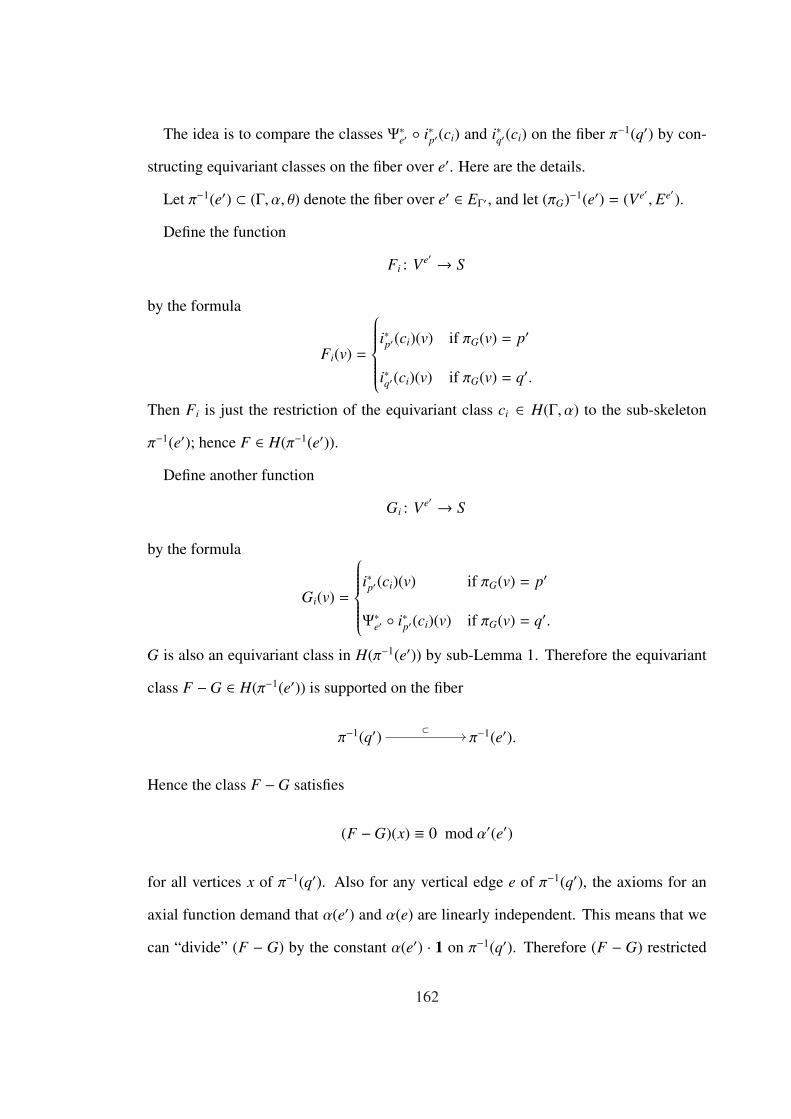
The idea is to compare the classes Ψ∗e′ ◦ i∗p′(ci) and i∗q′(ci) on the fiber π−1(q′) by con-

structing equivariant classes on the fiber over e′. Here are the details.

Let π−1(e′) ⊂ (Γ, α, θ) denote the fiber over e′ ∈ EΓ′ , and let (πG)−1(e′) = (Ve′ , Ee′).

Define the function

Fi : Ve′ → S

by the formula

Fi(v) =

i∗p′(ci)(v) if πG(v) = p′

i∗q′(ci)(v) if πG(v) = q′.

Then Fi is just the restriction of the equivariant class ci ∈ H(Γ, α) to the sub-skeleton

π−1(e′); hence F ∈ H(π−1(e′)).

Define another function

Gi : Ve′ → S

by the formula

Gi(v) =

i∗p′(ci)(v) if πG(v) = p′

Ψ∗e′ ◦ i∗p′(ci)(v) if πG(v) = q′.

G is also an equivariant class in H(π−1(e′)) by sub-Lemma 1. Therefore the equivariant

class F −G ∈ H(π−1(e′)) is supported on the fiber

π−1(q′) ⊂ // π−1(e′).

Hence the class F −G satisfies

(F −G)(x) ≡ 0 mod α′(e′)

for all vertices x of π−1(q′). Also for any vertical edge e of π−1(q′), the axioms for an

axial function demand that α(e′) and α(e) are linearly independent. This means that we

can “divide” (F − G) by the constant α(e′) · 1 on π−1(q′). Therefore (F − G) restricted

162

to H(π−1(q′)) is in S + ·H(π−1(q′)); this shows that the equivariant classes Ψγ ◦ i∗p′(ci) and

i∗q′(ci) represent the same ordinary class. Therefore since {Ψγ ◦ i∗p′(ci)}i are an S -basis, the

classes {i∗q′(ci)}i must also be an S -basis. �

We now return to the general case of a pseudo-fiber bundle. Another way to phrase

Theorem 4.2.6 is as follows: if H(π−1(p′)) is free and if the restriction homomorphism

ip′ : H(Γ, α)→ H(π−1(p′))

is surjective for every p′ ∈ VΓ′ , then for any S -module section

s : H(π−1(p′))→ H(Γ, α, θ)

of i∗p′ for any fixed p′ ∈ VΓ′ , the map

H(π−1(p′)) ⊗S H(Γ′, α′) Φ // H(Γ, α)

g ⊗ f // s(g) · π∗( f )

is an isomorphism of H(Γ′, α′)-modules (note that the condition that ip′ : H(Γ, α) →H(π−1(p′)) is surjective is equivalent to the existence of classes c1, . . . , cN ∈ H(Γ, α) that

restrict to a basis on every fiber since the condition that any classes in H(Γ, α) restrict to a

basis on a single fiber π−1(p′) cuts out a Zariski open set in H(Γ, α) which is non-empty if

i∗p′ is surjective). An important point here is that the map Φ is not a ring homomorphism

in general. If the restriction map

i∗p′ : H(Γ, α)→ H(π−1(p′))

actually admits an S -algebra section

s : H(π−1(p′))→ H(Γ, α),

163

then the map Φ is an isomorphism of S -algebras (where the S -algebra structure on the

tensor product is the standard one assigned to the tensor product over S of two S -

algebras). Hence as a corollary of Theorem 4.2.6 we get a Kunneth formula for the

equivariant cohomology ring of the direct product 1-skeleton.

Corollary 4.2.8. Let (Γ, α, θ) ⊂ Rn be the direct product 1-skeleton with “horizontal”

factor (Γ′, α′) ⊂ Rn and “vertical” factor (Γ0, α0) ⊂ Rn. Assume that H(Γ0, α0) is a free

S -module.

H(Γ0, α0) ⊗S H(Γ′, α′) Φ // H(Γ, α)

g ⊗ f // (π0)∗(g) · (π′)∗( f )

is an isomorphism of S -algebras.

Proof. The point here is that the restriction homomorphisms are always surjective;

ι∗p′ : H(Γ, α, θ)→ H(Γ0, α0, θ0)

has as a section the induced map of the other projection

(π0)∗ : H(Γ0, α0, θ0)→ H(Γ, α, θ).

By Theorem 4.2.6 Φ is an isomorphism of H(Γ′, α′)-modules; since (π0)∗ is a ring ho-

momorphism, Φ is a ring isomorphism. �

We will see in the next section that Theorem 4.2.6 also implies a decomposition theo-

rem for the equivariant cohomology of the blow-up of a 1-skeleton.

We will now deduce an analogous decomposition for the ordinary cohomology of the

total space of a fiber bundle. We will see that this is really just a formal consequence of

Theorem 4.2.6.

164

Theorem 4.2.9. Given a pseudo-fiber bundle

π−1(p′)ip′

// (Γ, α, θ)

π

²²

(Γ′, α′, θ′)

satisfying the hypotheses of Theorem 4.2.6, the map

H(π−1(p′)) ⊗R H(Γ′, α′)φ

// H(Γ, α)

ι∗p′(ci) ⊗ f // ci · π∗( f ).

is an isomorphism of H(Γ′, α′)-modules.

Proof. The map

H(π−1(p′)) ⊗S H(Γ′, α′) Φ // H(Γ, α)

ι∗p′(ci) ⊗ f // ci · π∗( f ).

(4.2.7)

is in particular an isomorphism of S -modules (where the tensor product is equipped with

the usual S -module structure assigned to the tensor product of two S -modules over S ).

Therefore we can just apply the functor − ⊗S S/S + both sides of (4.2.7) and use the

identification

(H(Γ′, α′) ⊗S H(π−1(p′))) ⊗S S/S + � (H(Γ′, α′) ⊗S S/S +) ⊗S/S + (H(π−1(p′)) ⊗S S/S +).


Thus we also get a Kunneth formula for the ordinary cohomology ring for the direct

product 1-skeleton by the same arguments.

165

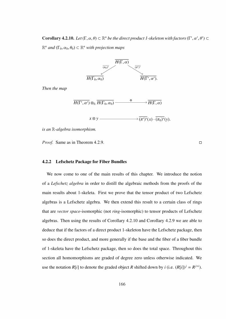
Corollary 4.2.10. Let (Γ, α, θ) ⊂ Rn be the direct product 1-skeleton with factors (Γ′, α′, θ′) ⊂Rn and (Γ0, α0, θ0) ⊂ Rn with projection maps

H(Γ, α)(π′)∗

%%KKKKKKKKKK(π0)∗

yyssssssssss

H(Γ0, α0) H(Γ′, α′).

Then the map

H(Γ′, α′) ⊗R H(Γ0, α0)Φ // H(Γ, α)

x ⊗ y // (π′)∗(x) · (π0)∗(y).

is an R-algebra isomorphism.

Proof. Same as in Theorem 4.2.9. �

4.2.2 Lefschetz Package for Fiber Bundles

We now come to one of the main results of this chapter. We introduce the notion

of a Lefschetz algebra in order to distill the algebraic methods from the proofs of the

main results about 1-skeleta. First we prove that the tensor product of two Lefschetz

algebras is a Lefschetz algebra. We then extend this result to a certain class of rings

that are vector space-isomorphic (not ring-isomorphic) to tensor products of Lefschetz

algebras. Then using the results of Corollary 4.2.10 and Corollary 4.2.9 we are able to

deduce that if the factors of a direct product 1-skeleton have the Lefschetz package, then

so does the direct product, and more generally if the base and the fiber of a fiber bundle

of 1-skeleta have the Lefschetz package, then so does the total space. Throughout this

section all homomorphisms are graded of degree zero unless otherwise indicated. We

use the notation R[i] to denote the graded object R shifted down by i (i.e. (R[i]) j = R j+i).

166

Definition 4.2.11. A Lefschetz algebra is a pair (R, l) consisting of anN-graded Artinian

R-algebra R together with a fixed Lefschetz element l ∈ R1 for R.

It will be convenient to think of the R-algebra R as a module over the polynomial ring

in one variable R[X] (with the usual grading), where X acts on R by multiplication by

l. In fact any degree one endomorphism A : R → R[1] defines a graded R[X]-module

structure on R by defining

Xi · r B Ai(r).

Definition 4.2.12. A Lefschetz module is a finite dimensional N-graded R[X]-module

M =⊕d

i=0 Mi such that the multiplication maps Xd−2i · m are isomorphisms for 0 ≤ i ≤b d

2c.

Thus a Lefschetz algebra (R, l) is a Lefschetz module R with a graded R-algebra struc-

ture whose X action is given by multiplication by the element l ∈ R1.

The simplest non-trivial example of a Lefschetz algebra is the polynomial ring in one

variable divided by a monomial:R[X]〈Xn+1〉 .

Here the fixed Lefschetz element is the equivalence class of X ∈ R[X]. These “simple”

Lefschetz algebras turn out to be the basic building blocks of all Lefschetz modules.

Definition 4.2.13. A simple Lefschetz algebra is (P(n), X) where

P(n) BR[X]〈Xn+1〉 .

Given a Lefschetz algebra (R, l), where R =⊕r

i=0 Ri, define the homogeneous sub-

space P ⊂ R where

Pi B ker{lr−2i+1 : Ri → Rr−i+1

}.

Note that for i > r2 , Pi = 0 The subspace P is called the primitive subspace of (R, l). We

have the following direct-sum decomposition of R.

167

Proposition 4.2.14. (Primitive Decomposition) There is an isomorphism of vector spaces

R =

b r2 c⊕

i=0

r−2i⊕

j=0

l j · Pi

.

Equivalently R is isomorphic (as Lefschetz modules) to a direct sum of shifted copies of

P(r − 2i) for 0 ≤ i ≤ b r2c:

R �b r

2 c⊕

i=0

pi · P(r − 2i)[i],

where pi = dimR(Pi).

Proof. To prove Proposition 4.2.14 we will show that

Ri = Pi ⊕ l(Pi−1) ⊕ . . . ⊕ li(P0)

for 0 ≤ i ≤ r. First we check that

Ri = Pi ⊕ l(Ri−1).

Let α ∈ Ri. If α ∈ Pi ∩ l(Ri−1) then α = l(β) and

lr−2i+1 · α = 0 = lr−2(i−1)β

and since

lr−2(i−1) : Ri−1 → Rr−(i−1)

is an isomorphism, we conclude that β and therefore α must be zero. Now fix α ∈ Ri and

consider the element

lr−2i+1 · α ∈ Rr−i+1 = Rr−(i−1).

Since lr−2(i−1) : Ri−1 → Rr−(i−1) is an isomorphism, there is a β ∈ Ri−1 such that

lr−2(i−1) · β = lr−2i+1 · α.

Hence

0 = lr−2i+1 · (α − l · β)

168

and thus α − l · β ∈ Pi. Therefore we can write α = (α − l · β) + l · β. This shows that

Ri = Pi ⊕ l(Ri−1).

To prove the proposition we use induction on i: The base case is trivial since R0 = P0.

Assuming that Ri−1 = Pi−1 ⊕ l(Pi−2) ⊕ . . . ⊕ li−1(P0) the result follows from the equation

Ri = Pi ⊕ l(Ri−1). By choosing a basis for the subspaces Pi we obtain the equivalent

decomposition

R �b r

2 c⊕

i=0

pi · P(r − 2i)[i].

This completes the proof of Proposition 4.2.14. �

The following lemma is due to Barthel, Brasselet, Fieseler and Kaup in [2].

Lemma 4.2.15. Let (U, µ) and (V, ν) be two Lefschetz algebras. Define the N-graded

Artinian R-algebra

W B U ⊗R V.

Let ω B µ ⊗ 1 + 1 ⊗ ν ∈ W1. Then (W, ω) is a Lefschetz algebra.

Proof. See [2], Proposition 5.7. �

We are now in a position to state and prove the main algebraic result of this section.

The proof relies on Lemma 4.2.15.

Theorem 4.2.16. Let (B, λ) and (F, τ) be Lefschetz algebras. Let W =⊕

i≥0 W i be an

N-graded Artinian R-algebra equipped with R-algebra homomorphisms

π : B→ W

and

ι : W → F.

Suppose that

169

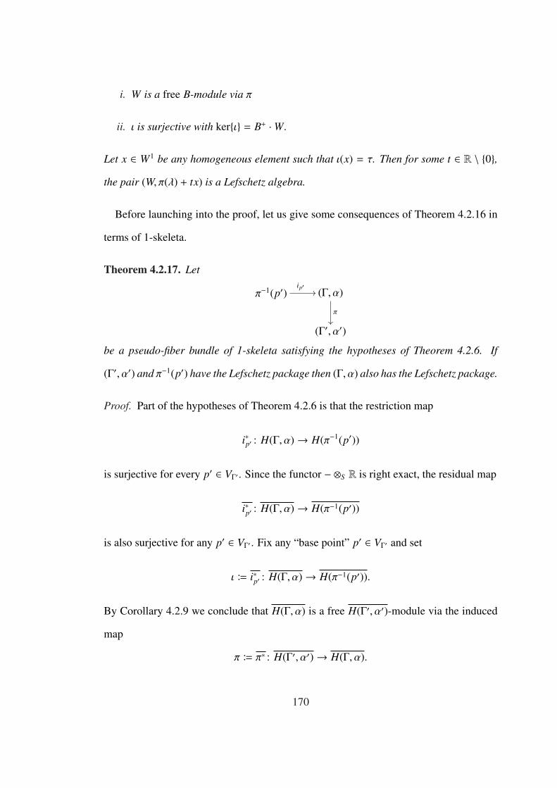
i. W is a free B-module via π

ii. ι is surjective with ker{ι} = B+ ·W.

Let x ∈ W1 be any homogeneous element such that ι(x) = τ. Then for some t ∈ R \ {0},the pair (W, π(λ) + tx) is a Lefschetz algebra.

Before launching into the proof, let us give some consequences of Theorem 4.2.16 in

terms of 1-skeleta.

Theorem 4.2.17. Let

π−1(p′)ip′

// (Γ, α)

π

²²

(Γ′, α′)

be a pseudo-fiber bundle of 1-skeleta satisfying the hypotheses of Theorem 4.2.6. If

(Γ′, α′) and π−1(p′) have the Lefschetz package then (Γ, α) also has the Lefschetz package.

Proof. Part of the hypotheses of Theorem 4.2.6 is that the restriction map

i∗p′ : H(Γ, α)→ H(π−1(p′))

is surjective for every p′ ∈ VΓ′ . Since the functor − ⊗S R is right exact, the residual map

i∗p′ : H(Γ, α)→ H(π−1(p′))

is also surjective for any p′ ∈ VΓ′ . Fix any “base point” p′ ∈ VΓ′ and set

ι B i∗p′ : H(Γ, α)→ H(π−1(p′)).

By Corollary 4.2.9 we conclude that H(Γ, α) is a free H(Γ′, α′)-module via the induced

map

π B π∗ : H(Γ′, α′)→ H(Γ, α).

170

Finally note that

ker{ι} = (H(Γ′, α′))+H(Γ, α) :

Since

ι∗p′ ◦ π∗ : H(Γ′, α′)→ H(π−1(p′))

has image the constant functions, we certainly have ⊇. Since H(Γ, α) is a free module

over H(Γ′, α′) on a basis that is an R-basis for H(π−1(p′)) the containment ⊆ follows from

dimension considerations; that is

dimR((H(Γ′, α′))+H(Γ, α)) = dimR(H(Γ′, α′)+) · dimR(H(Γ0, α0))

=(dimR(H(Γ′, α′)) − 1

)· dimR(H(Γ0, α0))

and

dimR(ker{ι}) = dimR(H(Γ, α)) − dimR(H(Γ0, α0))

= dimR(H(Γ′, α′)) · dimR(H(Γ0, α0)) − dimR(H(Γ0, α0))

=(dimR(H(Γ′, α′)) − 1

)· dimR(H(Γ0, α0)).

Therefore we can apply Theorem 4.2.16 where B = H(Γ′, α′), F = H(π−1(p′)) and

W = H(Γ, α). Since (Γ′, α′) and π−1(p′) have the Lefschetz package, Theorem 4.2.16

implies that (Γ, α) also has the Lefschetz package. This completes the proof of Theorem

4.2.17. �

Corollary 4.2.18. Let (Γ, α) denote the direct product 1-skeleton with factors (Γ′, α′)

and (Γ0, α0). Suppose that H(Γ0, α0) is a free S -module. If (Γ′, α′) and (Γ0, α0) have the

Lefschetz package then (Γ, α) also has the Lefschetz package.

171

Proof. Let

π′ : (Γ′, α′)→ (Γ, α)

and

π0 : (Γ0, α0)→ (Γ, α)

denote the natural projection morphisms. By Corollary 4.2.10 the map

H(Γ′, α′) ⊗R H(Γ0, α0)Φ // H(Γ, α)

x ⊗ y // (π′)∗(x) · (π0)∗(y)

is an isomorphism of R-algebras. By assumption there exist elements l′ ∈ H1(Γ′, α′) and

l0 ∈ H1(Γ0, α0) such that the pairs

(H(Γ′, α′), l′)

and

(H(Γ0, α0), l0)

are Lefschetz algebras. Then by Lemma 4.2.15 the pair

(H(Γ, α), (π′)(l′) + (π0)(l0))

is also a Lefschetz algebra. This completes the proof of Theorem 4.2.18. �

Corollary 4.2.18 could also have been deduced immediately from Lemma 4.2.15.

Proof of Theorem 4.2.16

The remainder of this section will be devoted to the proof of Theorem 4.2.16.

With notations as in the statement of Theorem 4.2.16, let B =⊕b

i=0 Bi and F =

⊕ fi=0 F i. Consider W as a B module via π and let End1

B(W) denote the graded B-module

172

endomorphisms of degree 1. Any choice of A ∈ End1B(W) endows W with a B[X]-module

structure by the prescription

(bXi) · w B b · (Ai(w)).

Also note that any R-vector space section (of degree zero)

s : F → W

of the surjective ring homomorphism ι (i.e. ι ◦ s = IF) yields a B-module isomorphism

B ⊗R F π⊗s // W

b ⊗ f // π(b) · s( f )

by conditions (i) and (ii), where the B-module structure on the tensor product is just

multiplication in the first factor.

Let us fix a section of ι : W → F as follows. First choose and fix any vector space

section (of degree zero)

s : F → W

and define the homogeneous subspace

P B s(P) ⊂ W

where P ⊂ F is the primitive subspace of the Lefschetz algebra (F, τ).

Define the homogeneous subspace

F =

b f2 c⊕

i=0

f−2i⊕

j=0

x j · Pi

⊂ W.

Define a new vector space section (of degree zero)

F s // W

τ j · pi // x j · s(pi)

173

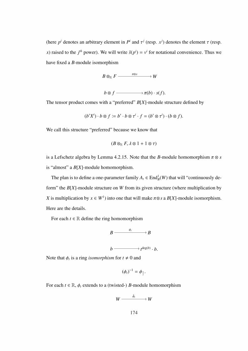
(here pi denotes an arbitrary element in Pi and τ j (resp. x j) denotes the element τ (resp.

x) raised to the jth power). We will write s(pi) = vi for notational convenience. Thus we

have fixed a B-module isomorphism

B ⊗R F π⊗s // W

b ⊗ f // π(b) · s( f ).

The tensor product comes with a “preferred” B[X]-module structure defined by

(b′Xi) · b ⊗ f B b′ · b ⊗ τi · f = (b′ ⊗ τi) · (b ⊗ f ).

We call this structure “preferred” because we know that

(B ⊗R F, λ ⊗ 1 + 1 ⊗ τ)

is a Lefschetz algebra by Lemma 4.2.15. Note that the B-module homomorphism π ⊗ s

is “almost” a B[X]-module homomorphism.

The plan is to define a one-parameter family At ∈ End1B(W) that will “continuously de-

form” the B[X]-module structure on W from its given structure (where multiplication by

X is multiplication by x ∈ W1) into one that will make π⊗ s a B[X]-module isomorphism.

Here are the details.

For each t ∈ R define the ring homomorphism

Bφt

// B

b // tdeg(b) · b.Note that φt is a ring isomorphism for t , 0 and

(φt)−1 = φ 1t.

For each t ∈ R, φt extends to a (twisted-) B-module homomorphism

Wφt

// W

174

in the sense that φt(b · w) = φt(b) · φt(w) for all b ∈ B and w ∈ W.

Define the vector space maps

At,i :f−2i⊕

j=0

x j · Pi → W[1]

by the formula

At,i(x j · s(vi)) =

x j+1 · vi if j < f − 2i

φt(x f−2i+1 · vi) if j = f − 2i.

For each t ∈ R this defines a vector space map

At Bb f

2 c⊕

i=0

At,i : F → W[1].

Since an R-basis for F is a B-module basis for W, these extend B-linearly to W to define

a one-parameter family

At : W → W[1]

of B-module endomorphisms as desired.

Lemma 4.2.19. There exist B-module homomorphisms χt : W → W (t ∈ R)such that the

following diagram commutes:

W

tx

²²

Wχt

oo

At

²²

W[1] W[1]χtoo

where the vertical map on the left is multiplication by the element tx ∈ W1.

Proof. Define for each t ∈ R the graded R-vector space maps

Fχt

// F

x j · vi // t j+ix j · vi.

175

These maps extend uniquely to B-module endomorphisms

Wχt // W

b · (x j · vi) // b · (t j+ix j · vi).

since W is free. The morphisms χt and φt are related by the following composition law

χt ◦ φt(w) = tdeg(w)w ∀t ∈ R. (4.2.8)

Now we need to show that χt ◦ At = (tx) · χt and it suffices to check this on (homoge-

neous) elements of W of the form b · (x j · vi). For t = 0 we compute

χ0 ◦ A0(b · (x j · vi)) =

b · 0 if j < f − 2i

b · χ0 ◦ φ0(x f−2i+1 · vi) if j = f − 2i

which is clearly zero in light of (4.2.8). For t , 0 the B-module homomorphisms χt are

actually B-module isomorphisms with

(χt)−1 = χ 1

t.

176

Hence we compute

χt ◦ At ◦ χ 1t(b · x j · vi) =χt ◦ At(

1t j+i b · x j · vi)

=

χt

(t− j−ib · x j+1 · vi

)if j < f − 2i

χt

(t− f +ib · φt(x f−2i+1 · vi)

)if j = f − 2i

=

tb · x j+1 · vi if j < f − 2i

t− f +ib · χt ◦ φt(x f−2i+1 · vi) if j = f − 2i

=

tb · x j+1 · vi if j < f − 2i

tb · (x f−2i+1 · vi) if j = f − 2i

=tx · (b · (x j · vi));

the second to last equality follows from (4.2.8). Hence

χt ◦ At ◦ χ 1t

= tx (4.2.9)

and the diagram commutes for every t ∈ R. This completes the proof of Lemma 4.2.19.

�

(4.2.9) can be interpreted as a B-module change of base formula for t , 0.

Lemma 4.2.20. At t = 0 there is another commutative diagram:

W

A0

²²

(B ⊗R F)π⊗soo

1⊗τ

²²

W[1] (B ⊗ F)[1].π⊗s

oo

177

Proof. As before, it suffices to check this for simple tensors of the form b ⊗ τ j pi where

τ j is the (fixed) Lefschetz element τ ∈ F1 raised to the jth power and pi is an arbitrary

element in Pi, the ith graded piece of the primitive subspace of the pair (F, τ).

We compute

A0 ◦ (π ⊗ s)(b ⊗ τ j pi) =

π(b) · x j+1s(pi) if j < f − 2i

π(b) · φ0(x f−2i+1s(pi)) if j = f − 2i.(4.2.10)

Recall that ι(x f−2i+1s(pi)) = τ f−2i+1 pi = 0, hence by assumption (ii), x f−2i+1s(pi) ∈ B+W;

but φ0(B+W) = 0. Applying this observation to (4.2.10) we get

A0 ◦ (π ⊗ s)(b ⊗ τ j pi) =

π(b) · x j+1s(pi) if j < f − 2i

0 if j = f − 2i.(4.2.11)

On the other hand we compute

(π ⊗ s) ◦ (1 ⊗ τ)(b ⊗ τ j pi) =

π(b) · x j+1s(pi) if j < f − 2i

0 if j = f − 2i.(4.2.12)

Hence the diagram commutes and this completes the proof of Lemma 4.2.20. �

We are now in a position to prove Theorem 4.2.16.

Proof of Theorem 4.2.16. Consider the R-vector space map

Λ + At ∈ End1R(W)

where

Λ : W → W[1]

is the map “multiplication by π(λ)”. Note that χt ◦ Λ = Λ ◦ χt for all t ∈ R. Assume for

the moment that for some fixed t , 0 and for each 0 ≤ k ≤ bw2 c, the map

(Λ + At)w−2k : Wk → Ww−k

178

is an isomorphism. Then by the commutivity of the diagram

W

π(λ)+tx

²²

Wχtoo

Λ+At

²²

W[1] W[1]χtoo

the pair (W, π(λ) + tx) is a Lefschetz algebra. Therefore it suffices to show that there is

some t , 0 such that

(Λ + At)w−2k : Wk → Ww−k

is an isomorphism for all 0 ≤ k ≤ bw2 c.

By the commutativity of the diagram

(B ⊗R F) π⊗s //

λ⊗1+1⊗τ

²²

W

Λ+A0

²²

(B ⊗ F)[1]π⊗s

// W[1]

and since

((B ⊗R F), λ ⊗ 1 + 1 ⊗ τ)

is a Lefschetz algebra (by Lemma 4.2.15), we deduce that for each 0 ≤ k ≤ bw2 c the maps

(Λ + A0)w−2k : Wk → Ww−k

are isomorphisms. Hence by the “principle of continuity” we conclude that there must

be some value of t0 different from zero such that the maps

(Λ + At0)w−2k : Wk → Ww−k

are isomorphisms (this “principle of continuity” can be made precise as follows: one first

observes that det((Λ + At)w−2k) is continuous in t (in fact it is a polynomial). Then since

179

det((Λ + A0)w−2k) is non-zero (by Lemma 4.2.15), one concludes that det((Λ + At)w−2k)

is not identically zero as a function of t; hence there is some value t0 , 0 such that

det((Λ + At0)w−2k) is non-zero). This proves that (W, π(λ) + t0x) is a Lefschetz algebra,

and hence completes the proof of Theorem 4.2.16. �

4.3 The Blow-Up

In this section we recall the notion of the blow-up of a 1-skeleton along a sub-skeleton.

This construction is due to Guillemin and Zara and we will try to adhere to their notation

in [14] as much as possible. In the first part we briefly recall this construction (from

chapter 2) and then describe a decomposition of the cohomology ring of the blow-up

(also due to Guillemin and Zara) in terms of the cohomology of the original 1-skeleta and

the sub-skeleton. We follow the same approach as in the case of fiber bundles: first prove

the result for equivariant cohomology, then derive the result for ordinary cohomology as

a formal consequence.

In the next part we prove an algebraic result that will imply, together with the de-

composition theorem above, that the blow-up of a 1-skeleton with the Lefschetz package

along a sub-skeleton with the Lefschetz package will itself have the Lefschetz package.

Fix a d-valent 1-skeleton with connection (Γ, α, θ) ⊂ Rn with compatibility system

{λe}e∈EΓand a k-valent totally geodesic, level sub-skeleton (Γ0, α0, θ0). Let N0 ⊂ EΓ

denote the oriented edges that are normal to Γ0. Since the sub-skeleton is level we choose

(and fix) a blow-up system, or a map

n : N0 → R+

180

that satisfy the condition that for every e ∈ E0 and every e′ ∈ N0

n(e)n(θe(e′))

= λe(e′).

Define the vertex set of Γ] to be

V] B VΓ \ V0 t N0.

Write ze to denote a vertex corresponding to an oriented edge e ∈ N0 or write zpe to denote

the vertex corresponding to e ∈ N0p.

There is a natural map of sets

β : V] → VΓ

defined by

β(x) =

q if x = q ∈ VΓ \ V0

p if x = ze for some e ∈ N0p

(4.3.1)

We declare two vertices x, y ∈ VΓ] to be adjacent if β(x) = β(y) or β(x)β(y) ∈ EΓ.

Denote this oriented edge set E].

There is a natural choice for connection θ] on Γ]. Furthermore, using the (fixed) blow-

up system n : N0 → R+ there is a natural choice for a (generalized) axial function α] for

the pair (Γ], θ]) defined by

α](ε) =

α(β(ε)) if ε) ∈ (E])h

n(e)α(e′) − n(e′)α(e) if ε = zeze′ ∈ (E])v.

(4.3.2)

For the remainder of this chapter, we will assume that α] is 2-independent (i.e. α] is an

axial function for (Γ], θ])).

The resulting 1-skeleton with connection (Γ], α], θ]) is called the blow-up of (Γ, α, θ)

along (Γ0, α0, θ0). Moreover the sub-graph Γ]0 ⊂ Γ] is the graph of a totally geodesic

sub-skeleton (Γ]0, α]0, θ

]0) called the singular locus of the blow-up.

181

The map β extends to a morphism of 1-skeleta with connections

β = (βG, InR) : (Γ], α], θ])→ (Γ, α, θ)

called the blow-down morphism (here we have used βG to denote the graph morphism

defined in (4.3.1)). The restriction of β to the singular locus

β0 : (Γ]0, α]0, θ

]0)→ (Γ0, α0, θ0)

is a pseudo-fiber bundle of 1-skeleta with connections whose fibers are complete 1-

skeleta on the (d − k) vertices corresponding to N0p, for p ∈ V0.

4.3.1 Cohomology of the Blow-Up

The singular locus is a level sub-skeleton (of co-valence 1) of the blow-up, hence there

is an equivariant Thom class τ ∈ H1(Γ], α]). A natural choice for such a Thom class is

the following:

τ(p) =

1n(e)α(e) if p = ze ∈ N0

0 otherwise.

Write τ0 ∈ H1(Γ]0, α]0) for the restriction of τ to the singular locus. For any equivariant

class h ∈ H(Γ]0, α]0), the class τ0 · h ∈ H(Γ]0, α

]0) can be “extended by zero” to a class on

(Γ], α]) that we express as τ ·h. We are abusing notation here slightly since h is not really

a class in H(Γ], α]); however if h extends to a class H ∈ H(Γ], α]), then we can write τ · has a “true” product of classes τ · H.

The blow-down morphism β : (Γ], α], θ]) → (Γ, α, θ) induces an inclusion of equivari-

ant cohomology rings

β∗ : H(Γ, α)→ H(Γ], α]),

and this gives H(Γ], α]) the structure of a H(Γ, α)-module. The image of β∗ in H(Γ], α])

is the set of classes that are constant over the fibers of β. The restriction of β to the

182

singular locus gives an inclusion

β∗0 : H(Γ0, α0)→ H(Γ]0, α]0),

and hence gives H(Γ]0, α]0) the structure of a H(Γ0, α0)-module. The natural inclusion

morphism

ρ : (Γ0, α0, θ0)→ (Γ, α, θ)

induces a restriction homomorphism

ρ∗ : H(Γ, α)→ H(Γ0, α0),

that gives H(Γ0, α0) the structure of a H(Γ, α)-module.

We have the following decomposition theorem for the equivariant cohomology of the

blow-up, due to Guillemin and Zara (cf. [14], Theorem 2.2.1).

Theorem 4.3.1. For every class F ∈ H(Γ], α]) there exist unique classes f0 ∈ H(Γ, α)

and gi ∈ H(Γ0, α0) such that

F = β∗( f0) +

d−k−1∑

i=1

β∗0(gi)τi,

where the classes in the sum on the right are classes in H(Γ]0, α]0) extended by zero to

classes in H(Γ], α]).

Equivalently, the map

H(Γ, α) ⊕(⊕d−k−1

i=1 H(Γ0, α0)τi0

)Ψ // H(Γ], α])

( f0,∑

giτi0) // β∗( f0) +

∑β∗0(gi)τi

(4.3.3)

is an H(Γ, α)-module isomorphism where the H(Γ, α)-module structure on the direct sum

is component wise-on the first factor by multiplication in H(Γ, α), and on the second

factor by restriction (via ρ∗)- and the H(Γ, α)-module structure on H(Γ], α]) is given by

β∗.

183

We will need the following lemma due to Guillemin and Zara in [16].

Lemma 4.3.2. Let (Γ′, α′) ⊂ Rn be a complete 1-skeleton on s vertices and let τ′ : VΓ′ →Rn be an injective function that is an equivariant class of degree 1 on (Γ′, α′). Then

{(τ′)i}s−1i=0 is an S -basis for H(Γ′, α′).

Proof. See [16], Theorem 4.1. �

Proof of Theorem 4.3.1. Fix v ∈ VΓ0 and set (Γ′, α′) = (β0)−1(v). Let τ′ : VΓ′ → Rn denote

the equivariant class of degree 1 that is the restriction of the Thom class τ0 ∈ H1(Γ]0, α]0)

to the fiber (β0)−1(v). By the definition of τ0, τ′ is an injective function, hence by Lemma

4.3.2 the classes

{(τ′)i}s−1i=0

are an S -basis for H(Γ′, α′), where s = d − k. Now we have a pseudo-fiber bundle of

1-skeleta with connections

(β0)−1(v)iv // (Γ]0, α

]0, θ

]0)

β0²²

(Γ0, α0, θ0),

and by Theorem 4.2.6 we deduce that {τi0}s−1

i=0 are a H(Γ0, α0)-basis for H(Γ]0, α]0). This

means that any class f ∈ H(Γ]0, α]0) can be written as

f =

s−1∑

i=0

β∗0(gi)τi0 (4.3.4)

for some unique gi ∈ H(Γ0, α0).

Now let F ∈ H(Γ], α]) be any equivariant class and let f ∈ H(Γ]0, α]0) be its restriction

to the singular locus. (4.3.4) gives

f =

s−1∑

i=0

β∗0(gi)τi0 = g0 +

s−1∑

i=1

β∗0(gi)τi0.

184

The second summand on the RHS can be “extended by zero” to an equivariant class

G Bs−1∑

i=1

β∗0(gi)τi ∈ H(Γ], α]). (4.3.5)

The class F −G ∈ H(Γ], α]) is constant on the fibers of β, hence we must have F −G =

β∗(F0) for some F0 ∈ H(Γ, α). This shows the existence of the decomposition.

To prove uniqueness, suppose that

β∗(F0) +

s−1∑

i=1

β∗0(gi)τi = 0

for some F0 ∈ H(Γ, α) and some gi ∈ H(Γ0, α0). Then its restriction to the singular locus

is also zero and Theorem 4.2.6 implies that the gi’s are all zero. Hence β∗(F0) = 0, but

β∗ is injective so we must have F0 = 0 as well.


Remark. If the restriction map ρ∗ : H(Γ, α)→ H(Γ0, α0) is surjective then for each i > 0

and each gi ∈ H(Γ0, α0), the class β∗0(gi)τi0 extends to a class β∗(Gi)τi where Gi ∈ H(Γ, α)

and ρ∗(Gi) = gi. In general it may not be possible to “divide by τi”. In the sequel, we

will assume that ρ∗ is surjective.

Corollary 4.3.3. The map

H(Γ, α) ⊕(⊕s

i=1 H(Γ0, α0)τi0

)Ψ // H(Γ], α])

( f0,∑

giτi0) // β∗( f0) +

∑β0∗(gi)τi

is an H(Γ, α)-module isomorphism.

Proof. Apply the functor − ⊗S R to both sides of (4.3.3). �

185

4.3.2 Lefschetz Package for the Blow-Up

We now come to the main result of this section. Following the same strategy as in

the case of fiber bundles, we break the result into two pieces: First, we give an alge-

braic result in the language of Lefschetz algebras. Then we show how this implies the

main result that says “the blow-up 1-skeleton of a 1-skeleton with the Lefschetz package

along a level sub-skeleton with the Lefschetz package also has the Lefschetz package”.

Throughout this section all homomorphisms are graded of degree zero unless otherwise

indicated. We use the notation R[i] to denote the graded object R shifted down by i (i.e.

(R[i]) j = R j+i).

For each n ≥ 0 let

P(n) B R[Y]/〈Yn〉 �n−1⊕

i=0

R · Y i

with the usual grading and

P+(n) Bn−1⊕

i=1

R · Y i,

the ideal generated by those elements of positive degree.

Let

B =

b⊕

i=0

Bi

and

U =

u⊕

j=0

U j

be N-graded Artinian R-algebras and let

ρ : U → B

be a graded R-algebra homomorphism. Define the N-graded ring

W B P+(s) ⊗R B �s−1⊕

k=1

Yk ⊗R B;

186

W is an ideal of the N-graded Artinian R-algebra P(s) ⊗R B that has the structure of a

free B-module with the basis {Yk}s−1k=1, where s + b = u. Set w = b + (s − 1) = u − 1; then

W =⊕w

k=1 Wk. The map ρ gives W the structure of a U-module, hence we can form the

direct sum of U-modules

U ⊕W;

this direct sum is naturally an N-graded Artinian R-algebra where multiplication is de-

fined by

(u,w) · (u′,w′) = (u · u′, u′ · w + u · w′ + w · w′).

Endow this direct sum with the standard U[X]-module structure by the prescription

X · (u,w) B (0,Y ⊗ ρ(u) + Y · w) = (0,Y · (1 ⊗ ρ(u) + w)). (4.3.6)

We have the following preliminary result.

Lemma 4.3.4. Suppose (B, λ) and (U,Λ) are Lefschetz algebras with

ρ(Λ) = λ.

Then (U ⊕W,Λ + X) is a Lefschetz algebra, where X is the operator in (4.3.6).

Proof. We need to show that the maps

(Λ + X)u−2m : (Um ⊕Wm)→ (Uu−m ⊕Wu−m) (4.3.7)

are isomorphisms for 0 ≤ m ≤ b u2c. The crucial observation to make is that the homoge-

neous subspace

{0} ⊕W ⊂ U ⊕W

is actually a U[X]-sub-module. Choose a homogeneous basis of U and a homogeneous

basis for W to get a homogeneous basis for the direct sum U⊕W. We compute the matrix

187

for the linear map (4.3.7) in terms of this basis: it has the form

Λu−2m 0

∗ (λ + Y)w−2m+1

.

Since we are assuming that the map

Λu−2m : Um → Uu−m

is an isomorphism, it suffices to prove that

(λ + Y)w−2m+1 : Wm → Ww−m+1 (4.3.8)

is an isomorphism (remember that u = w + 1 here).

Define the R[Y]-module isomorphism

P+(s) π // P(s − 1)[−1]

Y i // Y i−1.

(4.3.9)

This extends formally to a B[Y]-module isomorphism

W π // (P(s − 1) ⊗R B)[−1]

Y i ⊗ b // Y i−1 ⊗ b.

(4.3.10)

Thus we have the commutative diagram

Wm π

�//

(λ+Y)w−2m+1

²²

(P(s − 1) ⊗R B)m−1

(λ+Y)(w−1)−2(m−1)�

²²

Ww−m+1 π

�// (P(s − 1) ⊗R B)(w−1)−(m−1).

Lemma 4.2.15 implies that the right vertical map is an isomorphism, hence the left ver-

tical map must also be an isomorphism. Thus (4.3.8) is an isomorphism and therefore

(4.3.7) is an isomorphism. This completes the proof of Lemma 4.3.4. �

188

Remark. If the map ρ : U → B is surjective, and if U and B both have the strong

Lefschetz property, then it is always possible to find a Lefschetz element Λ ∈ U1 for U

such that ρ(Λ) = λ ∈ B1 is a Lefschetz element for B. Indeed the set of such Λ ∈ U1 is

the intersection of two non-empty Zariski-open sets.

Here is the main (algebraic) result.

Theorem 4.3.5. Let B, U, and W and be as in Lemma 4.3.4 and assume the R-algebra

map ρ : U → B is surjective. Let E =⊕

i≥0 Ei be an N-graded Artinian R-algebra and

suppose there is an R-algebra homomorphism β : U → E and a U-module homomor-

phism χ : W → E, (the U-module structure on E given by β) such that

i. χ(Y i ⊗ b) = χ(Y ⊗ 1) · χ(Y i−1 ⊗ b) for 1 < i < s

ii. the map

U ⊕Wβ⊕χ

// E

(u,w) // β(u) + χ(w)

is an isomorphism of U-modules. Then (E, β(Λ) + tχ(Y ⊗ 1)) is a Lefschetz algebra for

some t , 0, where Λ ∈ U1 is a Lefschetz element for U such that ρ(Λ) = λ ∈ B1 is

Lefschetz for B.

Proof. For notational convenience let

τ B χ(Y ⊗ 1) ∈ E1.

E is endowed with a “natural” U[X]-module structure by the prescription

(u · Xi) · e B β(u) · τi · e (4.3.11)

189

where the dots on the right hand side denote multiplication in E. Fix a homogeneous

R-vectorspace section σ : B → U of ρ (which exists since ρ is surjective). Note that for

any b ∈ B and 1 ≤ i ≤ s − 1 we have

χ(Y i ⊗ b) = β(σ(b)) · χ(Y i ⊗ 1) = β(σ(b)) · τi (4.3.12)

where the first equality follows from the assumption that χ is a U-module homomor-

phism, and the second follows from the assumption (i) in the statement of the theorem.

Furthermore any element A ∈ End1U(E) defines another U[X]-module structure on E by

(u · Xi) · e B β(u) · Ai(e).

The idea is to find a 1-parameter family At ∈ End1U(E) that will “continuously deform”

the U[X]-module structure on E from the “natural” one in (4.3.11) above to that of the

standard one on U ⊕W as in Lemma 4.3.4. Here are the details.

For each t ∈ R define the R-vector space map

EΦt // E

β(u) + χ(Y i ⊗ b) // tdeg(u)β(u) + tdeg(b)χ(Y i ⊗ b).

This map is well defined by (ii) in the statement of Theorem 4.3.5.

Next define, for each t ∈ R, the U-module homomorphism

EAt // E

by

At(β(u) + χ(Y i ⊗ b)) B β(u) · τ + β(σ(b)) · Φt(τi+1).

Note that for i < s − 1, Φt(τi+1) = τi+1. Thus for i < s − 1 applying At to β(u) + χ(Y i ⊗ b)

is the same as multiplying by τ.

190

Define the intermediary U-module homomorphisms

Eγt

// E

β(u) + χ(Y i ⊗ b) // β(u) + tiχ(Y i ⊗ b).

One can easily check that γt and Φt are related by the formula

γt ◦ Φt(e) = tdeg(e) · e ∀e ∈ E. (4.3.13)

The following claim establishes a relationship between the U[X]-module on E with re-

spect to multiplication by (R-multiples of) τ, and the U[X]-module structure on E with

respect to At ∈ End1U(E).

Claim. The following diagram commutes:

Etτ

²²

Eγt

oo

At²²

E[1] E[1]γt

oo

(4.3.14)

where the left vertical map is multiplication by the element tτ ∈ E1.

For t = 0 we have γ0 ◦ A0 = 0 = 0 · γ0. For t , 0 note that γt is an isomorphism and

that (γt)−1 = γ 1t. We compute:

For i < s − 1:

γt ◦ At ◦ γ 1t(β(u) + χ(Y i ⊗ b)) =γt ◦ At

(β(u) + t−iχ(Y i ⊗ b)

)

=γt

(β(u) · τ + t−iτ · χ(Y i ⊗ b)

)

=γt

(χ(Y ⊗ ρ(u)) + t−iχ(Y i+1 ⊗ b)

)

=t · χ(Y ⊗ ρ(u)) + t−i · ti+1χ(Y i+1 ⊗ b)

=tχ(Y ⊗ ρ(u)) + tχ(Y i+1 ⊗ b)

=tβ(u) · τ + tτ · χ(Y i ⊗ b).

191

For i = s − 1:

γt ◦ At ◦ γ 1t(β(u) + χ(Y s−1 ⊗ b)) =γt ◦ At

(β(u) + t−s+1χ(Y s−1 ⊗ b)

)

=γt

(β(u) · τ + t−s+1β(σ(b)) · Φt(τs)

)

=γt (χ(Y ⊗ ρ(u))) + t−s+1β(σ(b)) · γt ◦ Φt(τs)

=tχ(Y ⊗ ρ(u)) + tβ(σ(b)) · τs

=tβ(u) · τ + tτ · χ(Y s−1 ⊗ b).

This establishes the claim.

The next claim establishes a relationship between the standard U[X]-module structure

on U ⊕W and the U[X]-module structure on E with respect to A0 ∈ End1U(E).

Claim. The following diagram commutes

U ⊕W

X²²

β⊕χ// E

A0²²

(U ⊕W) [1]β⊕χ

// E[1]

(4.3.15)

where the left vertical map is multiplication by “X” as in (4.3.6).

The crucial observation here is that Φ0(τs) = 0. The point is that

τs = β(u) + χ

s−1∑

i=1

Y i ⊗ bi

where deg(u) = s > 0 and deg(bi) = s − i > 0.

192

We compute

A0

(β(u) + χ(Y i ⊗ b)

)=β(u) · τ +

τ · χ(Y i ⊗ b) if i < s − 1

β(σ(b)) · Φ0(τs) if i = s

=τ · β(u) +

β(σ(b)) · τi+1 if i < s − 1

0 if i = s

=χ(Y ⊗ ρ(u)) + χ(Y i+1 ⊗ b)

=β ⊕ χ(X · (u,Y i ⊗ b)

)

which establishes the claim.

We are now in a position to finish up the argument. Suppose that

E =

e⊕

l=0

El.

Then e = w + 1 = b + s. For fixed 0 ≤ m ≤ b e2c we want to show that the linear maps

(β(Λ) + tτ)e−2m : Em → Ee−m

are isomorphisms for some fixed value of t , 0. Note that for all t ∈ R we have

γt(β(Λ)) = β(Λ). Thus since (4.3.14) commutes the following diagram must also com-

mute:

E(β(Λ)+tτ)

²²

Eγt

oo

(β(Λ)+At)²²

E[1] E[1].γt

oo

Therefore it suffices to show that for some fixed value of t , 0, the maps

(β(Λ) + At)e−2m : Em → Ee−m (4.3.16)

are isomorphisms for all 0 ≤ m ≤ b e2c.

193

By the commutativity of the diagram in (4.3.15) the following diagram also commutes:

U ⊕W(Λ+X)

²²

β⊕χ// E

(β(Λ)+A0)²²

(U ⊕W)[1]β⊕χ

// E[1].

Therefore by Lemma 4.3.4 the maps in (4.3.16) must be isomorphisms for t = 0.

Hence by the “principle of continuity” there is some value t0 , 0 at which the maps

in (4.3.16) are isomorphisms. Therefore (E, β(Λ) + t0τ) is a Lefschetz algebra and this

completes the proof of Theorem 4.3.5. �

We use the above algebraic result to give the formulation of the main result in terms

of 1-skeleta and cohomology rings. As above we fix a d-valent 1-skeleton (Γ, α, θ) and a

k-valent sub-skeleton (Γ0, α0, θ0) and let (Γ], α], θ]) denote the blow-up of (Γ, α, θ) along

(Γ0, α0, θ0) using any fixed blow-up system n : N0 → R+. Let

β : (Γ], α], θ])→ (Γ, α, θ)

denote the blow-down morphism and let (Γ]0, α]0, θ

]0) be the singular locus. Let

ρ : (Γ0, α0, θ0)→ (Γ, α, θ)

denote the natural inclusion.

Here is the main result.

Theorem 4.3.6. Suppose that (Γ, α, θ) and (Γ0, α0, θ0) have the Lefschetz package. Fur-

thermore assume that the restriction map ρ∗ : H(Γ, α) → H(Γ0, α0) is surjective. Then

(Γ], α], θ]) also has the Lefschetz package.

Proof. Let

U B H(Γ, α)

B B H(Γ0, α0)

194

W Bs−1⊕

i=1

H(Γ0, α0)τi0

and

E B H(Γ], α]).

Let

ρ B ρ∗ : U → B

denote the restriction map and let

β B β∗ : U → E

denote the map induced from the blow-down morphism. Let

χ : W → E

denote the map “extension by zero” as in the assertion of Theorem 4.3.1. Note that χ is

a U-module homomorphism and since ρ∗ is surjective every class of the form β∗0(g) · τi0

extends by zero to a class of the form β(G) · τi. Thus χ satisfies condition (i) in the

statement of Theorem 4.3.5. Also by Theorem 4.3.3, the map

U ⊕Wβ⊕χ

// E

is an isomorphism of U-modules (so condition (ii) is also satisfied). Hence we can apply

Theorem 4.3.5 to conclude that (Γ], α], θ]) has the Lefschetz package with Lefschetz

element given by (β(Λ) + t0τ) ∈ H1(Γ], α]) for some t0 , 0, where Λ is a Lefschetz

element for U whose restriction ρ∗(Λ) is a Lefschetz element for B. This completes the

proof of Theorem 4.3.6. �

195

4.4 Applications To Coinvariant Rings

In this section we focus on the class of 1-skeleta arising from finite reflection groups.

Finite reflection groups are well studied objects in mathematics that are very rich in

structure. A finite reflection group comes equipped with an action on an ambient vector

space. This “geometric representation” of the group gives rise to a larger representation

on the polynomial ring, which in turn gives rise to the ring of invariant polynomials and

also the coinvariant ring. The coinvariant ring is the object of interest in this section. The

main goal is to prove that the coinvariant rings of certain finite reflection groups have

the strong Lefschetz property, or, equivalently (as we will show), to show that 1-skeleta

arising from these finite reflection groups have the Lefschetz package.

This section is split into two sub-sections. In the first sub-section we give a brief

overview of the theory of finite reflection groups (following [18]) and coinvariant rings

(following [17] and [3]) together with a description of the 1-skeleton of a finite reflec-

tion group (associated to a fixed root system). We will tie these two different points of

view together with a concrete isomorphism between the coinvariant ring of W and the

cohomology ring of the 1-skeleton of W. In the next sub-section we will prove an ana-

logue of Theorem 4.2.9 in the coinvariant setting. Then using Theorem 4.2.16 we give a

new proof of the fact that the coinvariant ring of W has the strong Lefschetz property for

several types, including the classical types A, B,C, and D.

4.4.1 Preliminaries

Fix an inner product 〈, 〉 on Rn. A reflection in Rn is a linear transformation sγ that

sends a vector γ to its negative and fixes the hyperplane orthogonal to γ pointwise. In

coordinates, we have

sγ(x) = x − γ(x)γ

196

for an appropriate co-vector γ ∈ (Rn)∗; in terms of the inner product we have γ(x) =

2 〈x,γ〉〈γ,γ〉 .

Definition 4.4.1. A (reduced) root system is a finite set of vectors Φ ⊂ Rn satisfying

R1. If α ∈ Φ then Rα ∩ Φ = {α,−α}

R2. If γ ∈ Φ then sγ(Φ) = Φ.

A set of roots ∆ ⊂ Φ is a simple system (with elements simple roots) if its elements

form a basis for spanR{Φ} ⊆ Rn and every element α ∈ Φ is a linear combination of

the simple roots with weights of the same sign. A root system always admits a simple

system. The rank of Φ is the number of simple roots in a simple system. A simple

system determines a set of roots Φ+ ⊂ Φ called the positive system (associated to the

simple system) by the condition that α ∈ Φ+ if α is a linear combination of the simple

roots with positive weights. The set of negative roots Φ− ⊂ Φ is defined analogously; we

have Φ = Φ+ t Φ−.

A finite reflection group W is a finite group that is generated by reflections. Note that

W is a finite subgroup of the orthogonal group on Rn.

Given a root system Φ ⊂ Rn, the finite reflection group W associated to Φ is the group

generated by the reflections corresponding to the roots: W = 〈sα | α ∈ Φ〉. Conversely

given a finite reflection group W an associated root system Φ ⊂ Rn is the set of unit

length generators (and their opposites) of the (−1)-eigenspaces of the reflections in W.

More precisely, let T ⊂ W be the set of reflections in W. For each reflection sγ ∈ T , let

the line Lγ ⊂ Rn denote its (−1)-eigenspace and let vγ ∈ Lγ be a unit vector. Then define

Φ = {±vγ | sγ ∈ T }. In general there are different choices for the length of generators of

the Lγ which will give rise to different root systems for the same finite reflection group.

For the remainder of this section, we fix a root system Φ ⊂ Rn, and a simple system

197

and its corresponding positive system ∆ ⊂ Φ+. Let W be the finite reflection group

associated to Φ. We collect some basic facts that will be needed in the sequel.

Label the simple roots ∆ = {γ1, . . . , γk} and let sk ∈ W denote the reflection corre-

sponding to the simple root γk. It turns out that the set of reflections S = {s1, . . . , sk} ⊂ W

generate W; these are called the simple reflections. Hence every element w ∈ W has an

expression as a word in the simple reflections.

Definition 4.4.2. For each w ∈ W define `(w) to be the smallest non-negative integer r

such that w = si1 · · · sir . We call the word si1 · · · sir reduced and we refer to the equality

w = si1 · · · sir as a reduced expression for w. The quantity `(w) is called the length of w.

Here are some basic properties of the length function.

Theorem 4.4.3. The length function ` : W → Z≥0 has the following properties:

i. There is a unique element w0 ∈ W of maximal length.

ii. `(u · v) ≤ `(u) + `(v) for all u, v ∈ W

iii. `(w0 · u−1) + `(u) = `(w0) for all u ∈ W

iv. `(u) = |Φ+ ∩ u−1(Φ−)| = |Φ+ ∩ u(Φ−)| = `(u−1) for all u ∈ W

v. `(sα · v) , `(v) for all α ∈ Φ+ and v ∈ W

vi. If γ ∈ ∆ then for all w ∈ W we have `(sγ · w) =

`(w) + 1 if w−1(γ) ∈ Φ+

`(w) − 1 if w−1(γ) ∈ Φ−

Proof. See [18], pages 12-16. �

The following is a fundamental property of the simple reflections.

Theorem 4.4.4. For α ∈ ∆, sα(Φ+ \ {α}) = Φ+ \ {α}.

198


For elements w′,w ∈ W we will write w′ α // w to mean that α ∈ Φ+, sα · w′ = w and

`(sα · w′) = `(w′) + 1. In general we have the following useful characterization of pairs

α ∈ Φ+ and w ∈ W such that `(sα · w) > `(w).

Theorem 4.4.5. For α ∈ Φ+, `(sα · w) > `(w) if and only if w−1(α) ∈ Φ+.


Remark. There is a natural partial order on the set W called the Bruhat ordering, de-

fined as follows: Set w ≤ w′ if and only if there exist group elements w1, . . . ,wN and

positive roots β0, . . . , βN such that

wβ0

// w1β1

// · · ·wNβN

// w′ .

Coinvariant Rings

The action of W on Rn induces an action of W on S = Sym(Rn), the symmetric algebra

of Rn or the polynomial ring on (Rn)∗. The set of polynomials that are invariant under this

action form a graded sub-ring S W ⊂ S called the invariant ring of W. Denote by I ⊂ S

the ideal generated by the invariant polynomials of positive degree: that is I = (S W)+ · S .

The quotient ring S/I is called the coinvariant ring of W. It is an interesting and difficult

problem to try and understand the ring structure of S/I. This is the starting point of

an active area of research known as “Schubert calculus”. In their famous paper [3],

Bernstein, I. Gel’fand, and S. Gel’fand introduced a set of operators on S that, among

other things, give a convenient description of the S W-module structure on S .

Definition 4.4.6. For γ ∈ Φ, define the operator Aγ : S → S [−1] by the formula

Aγ( f ) =f − sγ( f )

γ(4.4.1)

199

Since for x ∈ S 1 = Rn we have sγ(x) = x− γ(x)γ, the quotient x−sγ(x)γ

is the real number

γ(x). Since S is generated in degree one, it follows that Aγ is well-defined.

Theorem 4.4.7. The operator Aγ has the following properties:

i. A2γ = 0

ii. sγ = 1 − γ · Aγ

iii. ker(Aγ) = S 〈sγ〉

iv. Aγ(I) ⊂ I

Proof. See [17], Lemma 2.2. �

Given an expression w = si1 · · · sir (not necessarily reduced) define the operator

A(i1,...,ir) B Aγi1◦ · · · ◦ Aγir

: S → S [−r]. (4.4.2)

Theorem 4.4.8. ([3])

i. if `(w) < r (i.e. the expression w = si1 · · · sir is not reduced) then the operator

A(i1,...,ir) is zero.

ii. if `(w) = r (i.e. the expression w = si1 · · · sir is reduced) then the operator A(i1,...,ir)

depends only on the element w; it is independent of the reduced expression for w.

Proof. See [3], Theorem 3.4 or [17], Proposition 2.6. �

Define the BGG-operator for w, Aw : S → S [−r], to be the operator in (4.4.2) with

respect to any reduced expression; this is well defined by Theorem 4.4.8.

The following is a useful identity due to Bernstein, I. Gel’fand, and S. Gel’fand. In

fact this identity can be used to prove Theorem 4.4.8 in short order; see [3], Lemma 3.5

for more details. See also [17], Theorem 4.1.

200

Theorem 4.4.9. For each χ ∈ S 1 and each w ∈ W

[w−1 ◦ Aw, χ] =∑

w′α // w

α(w′(χ)) · w−1 ◦ Aw′ . (4.4.3)

Some explanation is in order here: on the LHS of (4.4.3) the element χ is viewed as the

operator χ : S → S [1] “multiplication by χ”. The element w ∈ W is similarly considered

as an operator w : S → S defined by its action on S . The symbol [X,Y] then denotes

the commutator of two operators X and Y on S . The sum is taken over all w′ ∈ W and

α ∈ Φ+ such that w′ α // w .

Set d = |Φ+|. Let ρ = 12

∑γ∈Φ+ γ ∈ S 1.

Lemma 4.4.10. Aw(ρ`(w)) > 0 for all w ∈ W.

Proof. We use induction on `(w) ≥ 0. The base case is trivial since Ae(ρ0) = Ae(1) =

1 > 0. Now assume the result holds for u ∈ W with `(u) < k and let w ∈ W be an element

of length k. Note that

Aw(ρ`(w)) =w−1 ◦ Aw(ρ`(w))

=[w−1 ◦ Aw, ρ](ρ`(w)−1) + ρ ◦(w−1 ◦ Aw

)(ρ`(w)−1) (4.4.4)

=[w−1 ◦ Aw, ρ](ρ`(w)−1).

The first equality in (4.4.4) holds since Aw(ρ`(w)) ∈ R is invariant under the action of W,

and the third equality follows from the fact that Aw(S k−1) = 0. Thus we apply (4.4.3) to

(4.4.4) to obtain the equality

Aw(ρ`(w)) =∑

w′α // w

α(w′(ρ)) · Aw′(ρ`(w′)). (4.4.5)

Therefore, by the induction hypothesis, it suffices to show that the quantity α(w′(ρ)) > 0

whenever α ∈ Φ+ and `(sα · w′) = `(w′) + 1. By Theorem 4.4.5, it suffices to verify that

β(ρ) > 0 whenever β ∈ Φ+.

201

To see this first fix α ∈ ∆ and consider the vector sα(ρ) B ρ − α(ρ)α. We can write

sα(ρ) = sα(ρ − 12α) + 1

2 sα(α). Note that sα(ρ − 12α) = ρ − 1

2α by Theorem 4.4.4; the point

is that ρ − 12α =

∑γ∈Φ+\{α} γ, and sα is a permutation of the set Φ+ \ {α}. Thus we see that

sα(ρ) = ρ − α = ρ − α(ρ)α. This shows that α(ρ) = 1 for all α ∈ ∆. Since the positve

roots are positive linear combinations of the simple roots it follows that β(ρ) > 0 for all

β ∈ Φ+. This completes the proof of Lemma 4.4.10. �

Lemma 4.4.11. For u, v ∈ W, we have

Au ◦ Av =

Au·v if `(u · v) = `(u) + `(v)

0 otherwise

Proof. This is an immediate consequence of Theorem 4.4.8. �

The following is known in the literature as the basis theorem. We will prove it here

since we will use the ideas of the proof later. We follow [3] Theorem 3.13 for the most

part (although our notation is slightly different). See [17] Theorem 2.7 for a different

proof.

Theorem 4.4.12. The elements {Aw(ρd) | w ∈ W} are a basis for the free S W-module S .

Proof. We first establish the S W-linear independence of the set {Aw(ρd) | w ∈ W}. Sup-

pose there is a non-trivial dependence relation

∑

w∈WcwAw(ρd) = 0, cw ∈ S W . (4.4.6)

Let v ∈ W be an element of minimal length such that cv , 0. Consider the operator

Aw0·v−1 . By Lemma 4.4.11 we have

Aw0·v−1 ◦ Au =

Aw0·v−1·u if `(w0 · v−1) + `(u) = `(w0 · v−1 · u)

0 otherwise

202

By Theorem 4.4.3 `(w0 ·v−1)+`(u) = d−`(v)+`(u) ≥ `(w0 ·v−1 ·u). Hence if `(u) > `(v),

the inequality is strict, and if `(u) = `(v) then we must have `(w0 ·v−1 ·u) = d hence u = v

(by the uniqueness of the longest word). Thus applying Aw0·v−1 to both sides of (4.4.6)

we get

cvAw0(ρd) = 0; (4.4.7)

note that Aw0·v−1 ◦ Au may not be zero for `(u) < `(v), but by our choice of v, the weight

cu will be zero. Since Aw0(ρd) > 0 by Lemma 4.4.10, (4.4.7) implies that cv = 0 which

contradicts our original assumption on cv. Therefore all the weights cw in (4.4.6) must

be zero and thus the set {Aw(ρd) | w ∈ W} is S W-linearly independent.

The argument that {Aw(ρd) | w ∈ W} generate S is a bit more involved. We will

argue by induction on k ≥ 0 that any element f ∈ S k can be expressed as an S W-

linear combination of the Aw(ρd)’s. The base case is trivial in light of Lemma 4.4.10:

this implies in particular that Aw0(ρd) , 0 hence f ∈ S 0 = R can be written as f =

1Aw0 (ρd) f · Aw0(ρ

d). Now assume any element of degree < k can be expressed as an S W-

linear combination of {Aw(ρd) | w ∈ W} and let f ∈ S be any homogeneous element of

degree k. We will show that f is I-equivalent to an element f ∈ spanR{Aw(ρd) | w ∈W, `(w) = d − k} ⊂ S k; the induction hypothesis will then finish the argument.

For each w ∈ W with `(w) = d − k, define the real number

cw BAw0·w−1( f )Aw0(ρd)

.

Set

f B∑

`(w)=d−k

cwAw(ρd) ∈ S k. (4.4.8)

Now apply the operator Aα (α ∈ ∆) to f and f : On the one hand, by the induction

hypothesis we get

Aα( f ) =∑

`(u)=d−k+1

cαu Au(ρd) +[higher terms

](4.4.9)

203

where the cαu ∈ R and the weights of the “higher terms” have degree > 0. On the other

hand we have by (4.4.8) and Lemma 4.4.11

Aα( f ) =∑

wα // u

cwAu(ρd). (4.4.10)

We would like to show that for u ∈ W, `(u) = d − k + 1 we have

cαu =

cw if w α // u

0 otherwise.(4.4.11)

First suppose that `(sα · u) > `(u). Then applying Aα to both sides of (4.4.9) again

yields

0 =∑

`(u)=d−k+1

uα // (sα · u)

cαu Asα·u(ρd) + “other terms”

where the “other terms” are of the form dαu · Aw′(ρd) where `(w′) > `(sα · u). Hence by

the S W-linear independence of the Aw(ρd)’s that we just established we see that indeed

cαu = 0.

On the other hand if `(sα ·u) < `(u) then we must have by Theorem 4.4.3 that `(sα ·u) =

`(u) − 1 and hence w = (sα · u) α // u . In this case applying the operator Aw0·u−1 to both

sides of (4.4.9) yields

Aw0·w−1( f ) = cαu Aw0(ρd) = cwAw0(ρ

d), (4.4.12)

hence in this case we get cαu = cw as desired (note that the higher terms in (4.4.9) are of

the form dαv · Av(ρd) where `(v) > d − k + 1, hence by Lemma 4.4.11, Aw0·u−1 ◦ Av is zero).

This shows that (4.4.11) holds.

Combining (4.4.11) with (4.4.9) and (4.4.10), we get Aα( f )−Aα( f ) =[higher terms

] ∈I and hence that Aα( f ) ≡ Aα( f ) mod I for every α ∈ ∆. This implies that

f − f ≡ sα( f − f ) mod I.

204

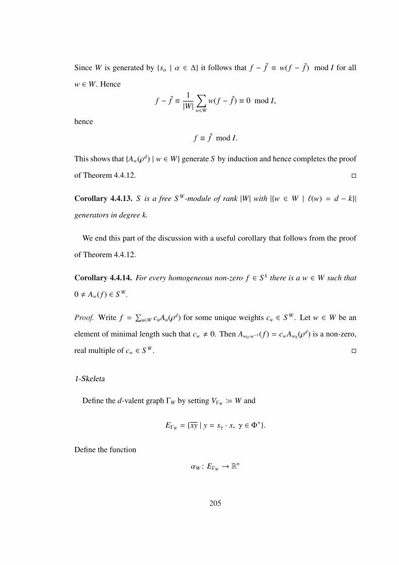
Since W is generated by {sα | α ∈ ∆} it follows that f − f ≡ w( f − f ) mod I for all

w ∈ W. Hence

f − f ≡ 1|W |

∑

w∈Ww( f − f ) ≡ 0 mod I,

hence

f ≡ f mod I.

This shows that {Aw(ρd) | w ∈ W} generate S by induction and hence completes the proof

of Theorem 4.4.12. �

Corollary 4.4.13. S is a free S W-module of rank |W | with |{w ∈ W | `(w) = d − k}|generators in degree k.

We end this part of the discussion with a useful corollary that follows from the proof

of Theorem 4.4.12.

Corollary 4.4.14. For every homogeneous non-zero f ∈ S k there is a w ∈ W such that

0 , Aw( f ) ∈ S W .

Proof. Write f =∑

u∈W cuAu(ρd) for some unique weights cu ∈ S W . Let w ∈ W be an

element of minimal length such that cw , 0. Then Aw0·w−1( f ) = cwAw0(ρd) is a non-zero,

real multiple of cw ∈ S W . �

1-Skeleta

Define the d-valent graph ΓW by setting VΓW B W and

EΓW = {xy | y = sγ · x, γ ∈ Φ+}.

Define the function

αW : EΓW → Rn

205

by the formula

α(x(sγ · x)) =

γ if x−1(γ) > 0

−γ if x−1(γ) < 0

It is straightforward to show that the pair (ΓW , αW) ⊂ Rn is a d-valent 1-skeleton. There

is a natural connection on ΓW compatible with αW , defined as follows. Fix e = x(sγ · x) ∈EΓW and let e′ B x(sβ · x) be any other oriented edge issuing from x. Define

θe(e′) B (sγ · x)(ssγ(β) · sγ · x).

We compute

αW(e) =

γ if x−1(γ) > 0

−γ if x−1(γ) < 0(4.4.13)

and

αW(e′) =

β if x−1(β) > 0

−β if x−1(β) < 0(4.4.14)

and

αW(θe(e′)) =

sγ(β) if x−1(γ) > 0

−sγ(β) if x−1(γ) < 0.(4.4.15)

Combining (4.4.14) and (4.4.15) with (4.4.13) we see that

α(e′) − α(θe(e′) = ±γ(β)α(e). (4.4.16)

Thus θW = {θe}e∈EΓWdefines a connection for the pair (ΓW , αW), hence we have a 1-

skeleton with connection (ΓW , αW , θW). Furthermore we see from (4.4.16) that the com-

patibility constants for (ΓW , αW , θW) are all equal to 1; in other words (ΓW , αW , θW) is

GKM.

It will be useful to fix a polarization of (ΓW , αW). Choose and fix a covector ξ ∈ (Rn)∗

such that 〈ξ, γ〉 > 0 for all γ ∈ ∆ (we can always choose such a covector since the

206

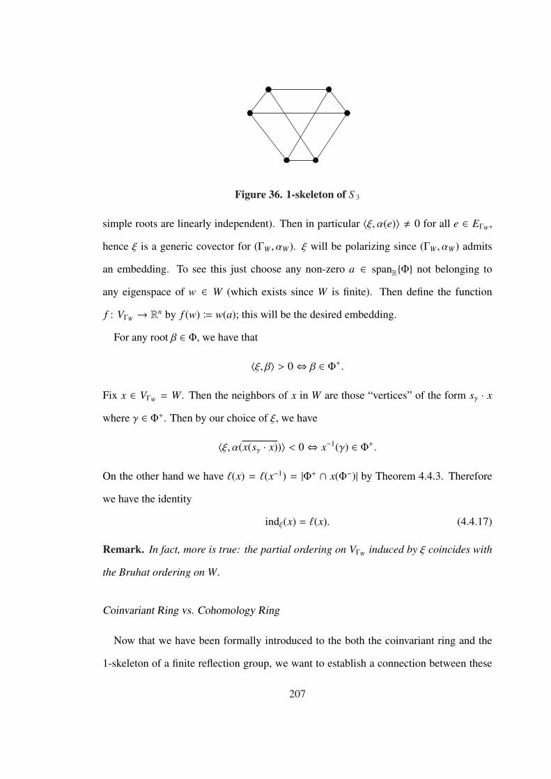
Figure 36. 1-skeleton of S 3

simple roots are linearly independent). Then in particular 〈ξ, α(e)〉 , 0 for all e ∈ EΓW ,

hence ξ is a generic covector for (ΓW , αW). ξ will be polarizing since (ΓW , αW) admits

an embedding. To see this just choose any non-zero a ∈ spanR{Φ} not belonging to

any eigenspace of w ∈ W (which exists since W is finite). Then define the function

f : VΓW → Rn by f (w) B w(a); this will be the desired embedding.

For any root β ∈ Φ, we have that

〈ξ, β〉 > 0⇔ β ∈ Φ+.

Fix x ∈ VΓW = W. Then the neighbors of x in W are those “vertices” of the form sγ · xwhere γ ∈ Φ+. Then by our choice of ξ, we have

〈ξ, α(x(sγ · x))〉 < 0⇔ x−1(γ) ∈ Φ+.

On the other hand we have `(x) = `(x−1) = |Φ+ ∩ x(Φ−)| by Theorem 4.4.3. Therefore

we have the identity

indξ(x) = `(x). (4.4.17)

Remark. In fact, more is true: the partial ordering on VΓW induced by ξ coincides with

the Bruhat ordering on W.

Coinvariant Ring vs. Cohomology Ring

Now that we have been formally introduced to the both the coinvariant ring and the

1-skeleton of a finite reflection group, we want to establish a connection between these

207

two objects. As usual, we will work with the equivariant cohomology ring of (ΓW , αW).

There is an “equivariant” coinvariant ring obtained by extending the scalars of the S W-

module S to a (right) S -module S ⊗S W S (i.e. s · ( f ⊗g) B f ⊗ s ·g for all s ∈ S and simple

tensors f ⊗ g ∈ S ⊗S W S ). By Theorem 4.4.12, S ⊗S W S is a free S -module of rank |W |.The BGG-operators Aw (which are S W-module endomorphisms of S ) extend formally

to operators Aw ⊗ 1 (now S -module endomorphisms of S ⊗S W S ); we will refer to these

extended operators as equivariant BGG-operators. There are analogous operators on the

equivariant cohomology of (ΓW , αW).

Definition 4.4.15. For each γ ∈ Φ and for each F : VΓW → S define the map

Zγ(F) : VΓW → Q(S )

by the formula

Zγ(F)(x) BF(x) − F(x · sγ)

x(γ)

where Q(S ) is the quotient field of S .

Lemma 4.4.16. If F ∈ H(ΓW , αW) then

i. Zγ(F)(x) ∈ S for all x ∈ W = VΓW ,

ii. The function Zγ(F) : VΓW → S is an equivariant class.

Proof. To see (i) we observe that for any γ ∈ Φ+ and any x ∈ W we have x · sγ = sx(γ) · x.

Hence if F ∈ H(ΓW , αW) then F(x) − F(x · sγ) ∈ 〈x(γ)〉 which implies that Zγ(F)(x) ∈ S .

To see (ii), let xy ∈ EΓW where y = sβ · x for some β ∈ Φ+. We have

Zγ(F)(x) =F(x) − F(x · sγ)

x(γ)(4.4.18)

Zγ(F)(y) =F(y) − F(y · sγ)

y(γ)(4.4.19)

208

We want to show that the difference Zγ(F)(x) − Zγ(F)(y) lies in the prime ideal 〈β〉 ⊂ S .

There are two cases to consider:

Case 1: x(γ) · y(γ) ∈ 〈β〉. Assume without loss of generality that x(γ) ∈ 〈β〉. Then

x(γ) = ±β, hence y = sβ · x = x · sx−1(β) = x · sγ. Thus in this case we have Zγ(F)(x) −Zγ(F)(y) = 0 ∈ 〈β〉.

Case 2: x(γ) · y(γ) < 〈β〉. In this case it will suffice to show that the product

(x(γ) · y(γ)) ·(Zγ(F)(x) − Zγ(F)(y)

)(4.4.20)

lies in the (prime) ideal 〈β〉. Expanding (4.4.20) we get

(F(x) − F(x · sγ)

)· y(γ) −

(F(y) − F(y · sγ)

)· x(γ)

=(F(x) − F(x · sγ)

)· (x(γ) − β(x(γ))β) −

(F(y) − F(y · sγ)

)· x(γ)

=[(F(x) − F(y)) −

(F(x · sγ) − F(y · sγ)

)]· x(γ) −

(F(x) − F(x · sγ)

)· β(x(γ))β.

Since F is an equivariant class, the first summand in the last equality lies in 〈β〉 and the

second is clearly in 〈β〉, hence (4.4.20) lies in 〈β〉. This proves that Zγ(F) is an equivariant

class. �

Thus it makes sense to define the S -module endomorphism Zγ : H(ΓW , αW)→ H(ΓW , αW)[−1].

There is a natural S -algebra homomorphism relating S ⊗S W S and H(ΓW , αW):

S ⊗S W S Ψ // H(ΓW , αW)

( f ⊗ g) // {x 7→ x( f ) · g} .

(4.4.21)

Lemma 4.4.17. The following diagram commutes

S ⊗S W S Ψ //

Aγ²²

H(ΓW , αW)

Zγ²²

S ⊗S W S [−1]Ψ

// H(ΓW , αW)[−1].

209

Proof. It is enough to check that Zγ ◦ Ψ = Ψ ◦ Aγ on the simple tensors in S ⊗S W S . We

compute:

Zγ(Ψ( f ⊗ g))(x) =x( f ) · g − x(sγ( f )) · g

x(γ)= g ·

(x( f ) − x(sγ( f ))

x(γ)

). (4.4.22)

On the other hand

Ψ(Aγ( f ⊗ g))(x) = x(

f − sγ( f )γ

)· g. (4.4.23)

Comparing (4.4.22) with (4.4.23) gives the desired result. �

Theorem 4.4.18. The map Ψ is an S -algebra isomorphism.

This is a non-trivial fact (although the proof is not difficult) relating two distinct points

of view of the same object: On the one hand the description of the equivariant cohomol-

ogy ring is local in nature; a class is determined by its value at the vertices. On the other

hand an element in S ⊗S W S is determined by the invariant theory of W on the polynomial

ring S .

Proof of Theorem 4.4.18. The first step is to compare the dimensions of the graded pieces.

From Theorem 4.4.12, S ⊗S W S is a free S -module with a basis {Aw(τ) ⊗ 1 | w ∈ W}. In

particular we compute directly that

dimR((S⊗S W S )k) =

k∑

i=0

|{x ∈ W | l(x) = d−k}|·dimR(S k−i) =

k∑

i=0

|{x ∈ W | l(x) = k}|·dimR(S k−i).

By (4.4.17) we see that

dimR((S ⊗S W S )k) =

k∑

i=0

bi(ΓW , αW) · dimR(S k−i). (4.4.24)

On the other hand, recall from the discussion in chapter 3 (see (3.1.3) on page 106)

that we always have the inequality

dimR(Hk(ΓW , αW)) ≤k∑

i=0

bi(ΓW , αW) · dimR(S k−i). (4.4.25)

210

Therefore in order to prove Theorem 4.4.18, it suffices to show that Ψ is injective.

Suppose otherwise and let f ∈ S ⊗S W S be a non-zero element in the kernel of Ψ.

By Corollary 4.4.14 there is a w ∈ W such that 0 , (Aw ⊗ 1)( f ) ∈ S W ⊗S W S . Then

Ψ((Aw ⊗ 1)( f )) : VΓW → S is a non-zero constant function. By Lemma 4.4.17 we deduce

that Zw(Ψ( f )) is the same non-zero constant function. But this contradicts our choice of

f ∈ ker{Ψ}. This shows that Ψ is injective and hence completes the proof of Theorem

4.4.18. �

Corollary 4.4.19. The map Ψ induces an isomorphism of graded R-algebras

Ψ : S W → H(ΓW , αW).

Proof. Apply the functor − ⊗S R to both sides of (4.4.21). �

Remark. An analogue of Theorem 4.4.18 is proved by Guillemin, Holm and Zara in the

case where W is a Weyl group, using ideas from equivariant cohomology theory applied

to homogeneous spaces. See [12] Theorem 2.6.

4.4.2 Leray-Hirsch Decomposition

In the interest of self-containment we will proceed without further mention of 1-

skeleta or cohomology rings. In this sub-section we establish a result analogous to The-

orem 4.2.9. We then use this result to deduce that S W has the strong Lefschetz property

for a certain class of finite reflection group W.

For any subset Θ ⊂ ∆ of simple roots, let ΦΘ ⊂ Φ denote the subset of roots in the

subspace spanned by Θ: ΦΘ = Φ∩spanR{Θ}. It is straightforward to show that ΦΘ is also

a root system of rank equal to |Θ|. A simple system for ΦΘ is Θ and Φ+ΘB Φ+∩spanR{Θ}

is the corresponding positive system. The reflection group WΘ associated to ΦΘ is a

subgroup of W called the parabolic subgroup associated to Θ. WΘ also acts on Rn and

211

thus on S by restricting the action of W. Let S WΘ denote the invariant ring of WΘ. Note

that the invariant ring of W is naturally a sub-ring of the invariant ring of WΘ. Let IΘ ⊂ S

denote the ideal generated by the positive degree invariants and let S WΘ= S/IΘ denote

the coinvariant ring of WΘ. Since I ⊆ IΘ, there is a natural surjection of rings

ι : S W → S WΘ

induced by the identity map on S .

The action of W on S induces an action on the coinvariant ring, S W , and hence by

restriction, an action by the parabolic sub-group WΘ. Let S WΘ

W denote the sub-ring of WΘ-

invariant coinvariants called the ring of relative coinvariants (with respect to WΘ ⊂ W).

Let

π : S WΘ

W → S W

denote the natural inclusion of rings.

We want to understand the relative coinvariants and their relation to the coinvariants.

First we give an alternative description that will be useful.

Lemma 4.4.20. The natural map i : S WΘ → S WΘ

W is surjective and induces an isomor-

phism S WΘ

(S W )+S WΘ� S WΘ

W .

Proof. To see that i is surjective, take any f ∈ S WΘ

W ⊂ S W and let F ∈ S be any lift. Let

F] ∈ S WΘ be the average of F over WΘ. Then i(F]) = f ] = f .

Note that ker(i) = (S W)+ · S ∩ S WΘ ⊇ (S W)+ · S WΘ . The claim is that the containment

is actually equality. Indeed let f ∈ ker(i); write f = s1g1 + . . .+ srgr for some s j ∈ (S W)+

and g j ∈ S . Averaging over WΘ we get f ] = f = s1g]1 + . . . + srg]r ∈ (S W)+ · S WΘ which

completes the proof. �

The following result is a version of Theorem 4.2.9 in the language of coinvariant rings.

212

Theorem 4.4.21. The coinvariant ring S W is a free S WΘ

W -module of rank |WΘ| = dimR(S WΘ).

Proof. By Corollary 4.4.13, S is a free S WΘ-module of rank |WΘ| B t. Therefore there is

an isomorphism of S WΘ-modules

Ψ : S →t⊕

i=1

S WΘ . (4.4.26)

Apply the functor − ⊗S W R to both sides of (4.4.26) to get

Ψ ⊗ 1: S ⊗S W R→

t⊕

i=1

S WΘ

⊗S W R �t⊕

i=1

(S WΘ ⊗S W R

).

By Lemma 4.4.20 S WΘ

W � S WΘ⊗S W R and this completes the proof of Theorem 4.4.21. �

Corollary 4.4.22. The surjection ι : S W → S WΘhas ker(ι) = (S WΘ

W )+ · S W

Proof. By Lemma 4.4.20 we have ker(ι) ⊇ (S WΘ

W )+S W ; we conclude that this containment

is an equality by dimension count: On the one hand we have

dim(ker(ι)) = dim(S W) − dim(S WΘ) = |W | − |WΘ|.

On the other hand by Theorem 4.4.21 we compute that dim(S WΘ

W ) = |WΘ| = |W ||WΘ | . There-

fore, again using Theorem 4.4.21, we compute

dim((S WΘ

W )+ · S W) =(|WΘ| − 1

)|WΘ| =

( |W ||WΘ| − 1

)|WΘ|.

This shows that ker(ι) = (S WΘ

W )+ · S W . �

We now take a closer look at the relative coinvariant ring itself. Let WΘ B {w ∈ W |l(w · sγ) = l(w) + 1 ∀γ ∈ Θ}.

Lemma 4.4.23. WΘ is the set of representatives of the cosets W/WΘ that have minimal

length. Furthermore, every element w ∈ W can be expressed uniquely as w = w ·w where

w ∈ WΘ and w ∈ WΘ and we have `(w) = `(w) + `(w).

213

Proof. See [17], Theorem 5.1 and Corollary 5.2. �

Define ρΘ = 12

∑γ∈Φ+

Θγ and ρ = 1

2

∑γ∈Φ+\Φ+

Θγ; we have ρ = ρΘ + ρ. Note that ρ ∈ S WΘ .

Indeed if α ∈ Θ ⊆ ∆ then

sα(Φ+Θ \ {α}) = Φ+

Θ \ {α}.

But also

sα(Φ+ \ {α}) = Φ+ \ {α}.

Therefore we must also have

sα(Φ+ \ Φ+Θ) ⊆ Φ+ \ Φ+

Θ.

Since WΘ is generated by sα (α ∈ Θ), we see that WΘ just permutes the roots in Φ+ \Φ+Θ

,

hence preserves ρ.

We write uβ

// w to mean that β ∈ Φ+, sβu = w and `(sβ · u) = `(u) + 1.

Lemma 4.4.24.

Aw(ρ`(w)) =∑

uβ

// w

β(u(ρ)) · Au(ρ`(u)), (4.4.27)

where the sum is taken over all u ∈ WΘ, β ∈ Φ+ such that uβ

// w

Proof. Use the identity in (4.4.5) to get

Aw(ρ`(w)) =∑

u α // w

α(u(ρ)) · Au(ρ`(u)). (4.4.28)

For u α // w write u = u · u as in Lemma 4.4.23. Then Au = Au ◦ Au. But for u , e,

Au(ρl(u)) = 0 since ρ is WΘ-invariant (we are appealing to Theorem 4.4.7 (iii) here).

Therefore the only non-zero summands in (4.4.28) are those for which u = u, hence the

assertion of Lemma 4.4.24 follows. �

214

Remark. A result of Deodhar (see [8], Corollary 3.8) states that given two elements

w1, w2 ∈ WΘ with w1 ≤ w2 (where ≤ denotes the Bruhat ordering on W), there exsist

elements u1, . . . , ur ∈ WΘ such that

w1 = u0β0

// u1β1

// · · · urβr

// ur+1 = w2 .

In particular this guarantees that the sum in (4.4.27) is never vacuous.

Lemma 4.4.25. α(ρ) > 0 for all α ∈ Φ+ \ Φ+Θ

.

Proof. First assume that α ∈ ∆ \ Θ. Then α(ρΘ) < 0 since 〈α, α′〉 < 0 for α′ ∈ ∆ \ {α}.On the other hand we have already seen that α(ρ) > 0, hence we must have α(ρ) > 0.

Now let α ∈ Φ+ \ Φ+Θ

be arbitrary. There is a unique αΘ ∈ spanR{Θ} such that

α =∑

γ∈∆\Θcγ · γ + αΘ

for some cγ ≥ 0. Since ρ is WΘ-invariant, we must have 〈αΘ, ρ〉 = 0. Thus we have that

〈α, ρ〉 =∑

γ∈∆\Θcγ · 〈γ, ρ〉. (4.4.29)

Using the formula

α(x) = 2〈α, x〉〈α, α〉

it follows from the argument above that 〈γ, ρ〉 > 0 for every γ ∈ ∆ \ Θ. Hence (4.4.29)

implies that 〈α, ρ〉 > 0 and therefore that α(ρ) > 0 for all α ∈ Φ+ \ Φ+Θ

as desired.

�

Lemma 4.4.26.

Aw(ρ`(w)) > 0. (4.4.30)

Proof. By (4.4.27) in Lemma 4.4.24 it suffices to show by induction that β(u(ρ)) > 0

for uβ

// w . By Theorem 4.4.5 uβ

// w implies that u−1(β) ∈ Φ+ \ Φ+Θ

. Indeed Theorem

215

4.4.5 certainly guarantees that u−1(β) ∈ Φ+. Since sβ · u = w = u · su−1(β) ∈ WΘ, the root

u−1(β) must not belong to Φ+Θ

.

By Lemma 4.4.25 we know that α(ρ) > 0 for all α ∈ Φ+ \ Φ+Θ

. We have

β(u(ρ)) =〈β, u(ρ)〉〈β, β〉 =

〈u−1(β), ρ〉〈u−1(β), u−1(β)〉 = α(ρ),

where we set α B u−1(β) ∈ Φ+ \ Φ+Θ

. Hence β(u(ρ)) > 0 as desired. �

Let us pause for a moment to take stock of what we have. Given any parabolic sub-

group WΘ ⊆ W, there is a natural inclusion

π : S WΘ

W → S W

with respect to which S W is a free S WΘ

W -module. There is a natural surjective ring homo-

morphism

ι : S W → S WΘ

whose kernel is the ideal (S WΘ

W )+ · S W . Thus if we knew that S WΘand S WΘ

W both had the

strong Lefschetz property, then we could deduce by Theorem 4.2.16 that S W also has the

Lefschetz property. Before we give the main result, we need a bit more terminology.

Let R =⊕d

i=0 Ri be an N-graded Artinian R-algebra. If ri B dimR(Ri) then define gi =

ri − ri−1 for 1 ≤ i ≤ b d2c. Define the g-vector of R to be the tuple g(R) B (g1, . . . , gb d−1

2 c).

If R has the strong Lefschetz property, the entries of the g-vector are the dimensions of

the positive graded pieces of the primitive subspace with respect to any given Lefschetz

element. For instance in the special case that g(R) is the zero vector, R has the strong

Lefschetz property if and only if there is an element l ∈ R1 such that ld , 0; in this case

the primitive subspace only exists in degree 0. In the literature the g-vector of a graded

ring R =⊕d

i=0 Ri is usually taken to be the tuple (g0, g1, . . . , gb d2 c), where g0 B 1; here

we just “cut off” the terms that we do not need.

Define the rank of W to be the rank of its associated root system Φ.

216

Definition 4.4.27. A finite reflection group W of rank N acting on S (Rn) = S is called

tight if there exists a chain of parabolic sub-groups

{e} ⊆ W1 ⊆ · · · ⊆ WN = W

such that

i. The rank of Wi is i

ii. g(S WiWi+1

) is the zero vector.

The main result is this:

Theorem 4.4.28. If W is tight then S W has the strong Lefschetz property.

Proof. The proof is by induction on the rk(W) ≥ 1.

For rk(W) = 1 we have W = {sγ, e} for some γ ∈ Rn. Then if we choose a basis

x1, . . . , xn−1 for the orthogonal complement of γ, we can write

S = R[x1, . . . , xn−1, γ]

and

S W = R[x1, . . . , xn−1, γ2].

Therefore we see that

S W =R[x1, . . . , xn−1, γ](x1, . . . , xn−1, γ2)

�R[γ]γ2 � P(2)

hence S W has the strong Lefschetz property.

Now assume the assertion holds for tight reflection groups of rank (k−1), and let W be

a tight reflection group of rank k. Since W is tight, there is a parabolic subgroup W ′ ⊂ W

that is also a tight reflection group of rank (k−1). Let W ⊂ W be the set of minimal coset

representatives of W/W ′ and let r = `(w0), the length of the longest element of W. By

217

Lemma 4.4.26 we know that Aw0(ρr) , 0, hence in particular ρr ∈ S W′ is not in the ideal

(S W)+ ·S W′; thus Lemma 4.4.20 implies that its equivalence class[ρ]r ∈ S W′

W is non-zero.

Since g(S W′W ) is the zero vector, we conclude that S W′

W has the strong Lefschetz property,

with Lefschetz element given by[ρ] ∈

(S W′

W

)1. By the induction hypothesis, S W′ has

the strong Lefschetz property. Hence by Theorem 4.2.16 (with B = S W′W , F = S W′ and

E = S W) S W also has the strong Lefschetz property. Thus by induction, S W has the

strong Lefschetz property for all tight finite reflection groups W. This completes the

proof of Theorem 4.4.28. �

Theorem 4.4.29. A finite reflection group is tight if and only if it is of type AN , BN �

CN ,DN , I2(m) or H3 as well as the rank 1 type that we call J1.

Proof. This can be checked directly using the fundamental weights of a finite reflection

group (see the table on page 59 in [18]) and the factorization of the Poincare polynomial

of the relative coinvariant ring (see Cor. 4.5 on page 154 of [17]). �


The main question underlying this chapter is the following:

Question. Which 1-skeleta have the Lefschetz package?

This question may not be tractable. While we have many examples of 1-skeleta that

have the Lefschetz package, the only examples we have at present of 1-skeleta that do

not have the Lefschetz package are those whose Betti numbers are not symmetric.

Problem. Find an example of a 1-skeleton with symmetric Betti numbers that does not

have the Lefschetz package.

218

In answering the above question it may be helpful to restrict the class of 1-skeleta. For

instance one can specialize the question as follows:

Question. Which 3-independent non-cyclic 1-skeleta have the Lefschetz package?

In this case, the classification result of Guillemin and Zara tells us that the Betti num-

bers are symmetric. Using the techniques of cutting and reduction as in chapter 2, one

realizes every such 1-skeleton as a cross-section of some larger 1-skeleton. This implies

that such a 1-skeleton is gotten from a very simple 1-skeleton by a finite sequence of

blow-ups and blow-downs. This would seem to be a viable strategy for answering this

specialized question in light of Theorem 4.3.6. We are only missing the converse:

Conjecture 2. If (Γ], α], θ]) has the Lefshcetz package, then (Γ, α, θ) also has the Lef-

schetz package.

The deformation arguments used in the proof of Theorem 4.3.6 do not directly apply

to Conjecture 2. It would seem that one needs a new idea here.

Regarding coinvariant rings of finite reflection groups and Theorems 4.4.28 and 4.2.17,

a natural question to ask is:

Question. Can these methods be used to extend the results of Theorem 4.4.28 to other

types of finite reflection groups?

There are only five types that are not tight as in Definition 4.4.27: E6, E7, E8, F4 and

H4. Of these the first four are crystallographic, hence in these cases, that S W has the

strong Lefschetz property follows from Theorem 4.1.1. So in some sense H4 is the most

interesting case. It was shown in 2007 by Numata and Wachi in [24] that S W has the

strong Lefschetz property for W of type H4. Their proof is essentially a computation

using the computer-algebra tool Macaulay2. We therefore feel that there is still room

for a more conceptual proof of this fact and Theorem 4.2.16 may provide one way to

219

do this. For W of type H4, there is a parabolic subgroup W ′ ⊆ W of type H3. Theorem

4.4.29 implies that S W′ has the strong Lefschetz property, hence by Theorem 4.2.16 it

suffices to show that S W′W has the strong Lefschetz property. We compute the Poincare

polynomial for S W′W to give the reader an idea of the task at hand:

P(W,W ′) =

(t2−1)(t12−1)(t20−1)(t30−1)(t−1)4

(t2−1)(t6−1)(t10−1)(t−1)3

= (t29 + t28 + . . . + t + 1)(t16 + t10 + t6 + 1)

=t45 + . . . + t40 + 2t39 + . . . + 2t36+

3t35 + . . . + 3t30 + 4t29 + . . . + 4t16 + 3t15 + . . . + 3t10+ (4.5.1)

2t9 + . . . + 2t6 + t5 + . . . + t + 1.

Hence the g-vector consists of three 1’s and ten 0’s. This indicates that there are three

additional primitive elements to be found in S W′W besides the natural primitive element in

degree zero.

The cases F4 and E6 are a little more promising in that we need only find one additional

primitive element. The case E7 is a little worse with two additional primitive elements

to find and E8 is the worst with seven(!).

220

BIBLIOGRAPHY

[1] Michele Audin. The topology of torus actions on symplectic manifolds, volume 93of Progress in Mathematics. Birkhauser Verlag, Basel, 1991. Translated from theFrench by the author.

[2] Gottfried Barthel, Ludger Kaup, J.-P. Brasselet, and Karl-Heinz Fieseler. Hodge-Riemann relations for polytopes: a geometric approach. In Singularity theory,pages 379–410. World Sci. Publ., Hackensack, NJ, 2007.

[3] I. N. Bernsteın, I. M. Gelfand, and S. I. Gelfand. Schubert cells, and the cohomol-ogy of the spaces G/P. Uspehi Mat. Nauk, 28(3(171)):3–26, 1973.

[4] Raoul Bott and Loring W. Tu. Differential forms in algebraic topology, volume 82of Graduate Texts in Mathematics. Springer-Verlag, New York, 1982.

[5] Theodore Chang and Tor Skjelbred. The topological Schur lemma and relatedresults. Ann. of Math. (2), 100:307–321, 1974.

[6] Henry Crapo and Walter Whiteley. Autocontraintes planes et polyedres projetes.I. Le motif de base. Structural Topology, (20):55–78, 1993. Dual French-Englishtext.

[7] Thomas Delzant. Hamiltoniens periodiques et images convexes de l’applicationmoment. Bull. Soc. Math. France, 116(3):315–339, 1988.

[8] Vinay V. Deodhar. Some characterizations of Bruhat ordering on a Coxeter groupand determination of the relative Mobius function. Invent. Math., 39(2):187–198,1977.

[9] William Fulton. Introduction to toric varieties, volume 131 of Annals of Mathe-matics Studies. Princeton University Press, Princeton, NJ, 1993. The William H.Roever Lectures in Geometry.

[10] Mark Goresky, Robert Kottwitz, and Robert MacPherson. Equivariant cohomology,Koszul duality, and the localization theorem. Invent. Math., 131(1):25–83, 1998.

[11] Branko Grunbaum. Convex polytopes, volume 221 of Graduate Texts in Mathemat-ics. Springer-Verlag, New York, second edition, 2003. Prepared and with a prefaceby Volker Kaibel, Victor Klee and Gunter M. Ziegler.

221

[12] V. Guillemin, T. Holm, and C. Zara. A GKM description of the equivariant coho-mology ring of a homogeneous space. J. Algebraic Combin., 23(1):21–41, 2006.

[13] V. Guillemin and C. Zara. Equivariant de Rham theory and graphs. Asian J. Math.,3(1):49–76, 1999. Sir Michael Atiyah: a great mathematician of the twentiethcentury.

[14] V. Guillemin and C. Zara. 1-skeleta, Betti numbers, and equivariant cohomology.Duke Math. J., 107(2):283–349, 2001.

[15] Victor Guillemin. Moment maps and combinatorial invariants of Hamiltonian T n-spaces, volume 122 of Progress in Mathematics. Birkhauser Boston Inc., Boston,MA, 1994.

[16] Victor Guillemin and Catalin Zara. The existence of generating families for thecohomology ring of a graph. Adv. Math., 174(1):115–153, 2003.

[17] Howard L. Hiller. Schubert calculus of a Coxeter group. Enseign. Math. (2), 27(1-2):57–84, 1981.

[18] James E. Humphreys. Reflection groups and Coxeter groups, volume 29 of Cam-bridge Studies in Advanced Mathematics. Cambridge University Press, Cambridge,1990.

[19] Katsuo Kawakubo. The theory of transformation groups. The Clarendon PressOxford University Press, New York, japanese edition, 1991.

[20] A. A. Klyachko. Equivariant bundles over toric varieties. Izv. Akad. Nauk SSSRSer. Mat., 53(5):1001–1039, 1135, 1989.

[21] Dusa McDuff and Dietmar Salamon. Introduction to symplectic topology. OxfordMathematical Monographs. The Clarendon Press Oxford University Press, NewYork, second edition, 1998.

[22] Peter McMullen. On simple polytopes. Invent. Math., 113(2):419–444, 1993.

[23] William Messing. Short sketch of Deligne’s proof of the hard Lefschetz theorem.In Algebraic geometry (Proc. Sympos. Pure Math., Vol. 29, Humboldt State Univ.,Arcata, Calif., 1974), pages 563–580. Amer. Math. Soc., Providence, R.I., 1975.

[24] Yasuhide Numata and Akihito Wachi. The strong Lefschetz property of the coin-variant ring of the Coxeter group of type H4. J. Algebra, 318(2):1032–1038, 2007.

[25] Christian Okonek, Michael Schneider, and Heinz Spindler. Vector bundles on com-plex projective spaces, volume 3 of Progress in Mathematics. Birkhauser Boston,Mass., 1980.

222

[26] Richard P. Stanley. The number of faces of a simplicial convex polytope. Adv. inMath., 35(3):236–238, 1980.

[27] V. A. Timorin. An analogue of the Hodge-Riemann relations for simple convexpolyhedra. Uspekhi Mat. Nauk, 54(2(326)):113–162, 1999.

[28] Catalin Zara Victor Guillemin, Silvia Sabatini. Cohomology of gkm fiber bundles.arXiv:0806.3539.

[29] Gunter M. Ziegler. Lectures on polytopes, volume 152 of Graduate Texts in Math-ematics. Springer-Verlag, New York, 1995.

223

Geometric and Combinatorial Aspects of 1-Skeleta

Documents