Geomechanics in Depleted Faulted Reservoirs - MDPI

energies

Article

Geomechanics in Depleted Faulted Reservoirs

Nikolaos Markou 1,2,* and Panos Papanastasiou 1

�����������������

Citation: Markou, N.; Papanastasiou,

P. Geomechanics in Depleted Faulted

Reservoirs. Energies 2021, 14, 60.

https://dx.doi.org/10.3390/en14010060

Received: 17 November 2020

Accepted: 19 December 2020

Published: 24 December 2020

Publisher’s Note: MDPI stays neu-

tral with regard to jurisdictional claims

in published maps and institutional

affiliations.

Copyright: © 2020 by the authors. Li-

censee MDPI, Basel, Switzerland. This

article is an open access article distributed

under the terms and conditions of the

Creative Commons Attribution (CC BY)

license (https://creativecommons.org/

licenses/by/4.0/).

1 Department of Civil and Environmental Engineering, University of Cyprus, Nicosia 1678, Cyprus;[email protected]

2 Hydrocarbons Service, Ministry of Energy, Commerce and Industry, Nicosia 1421, Cyprus* Correspondence: [email protected]

Abstract: This paper examines the impact of the effective stresses that develop during depletion of afaulted reservoir. The study is based on finite element modeling using 2D plane strain deformationanalysis with pore pressure and elastoplastic deformation of the reservoir and sealing shale layersgoverned by the Drucker–Prager plasticity model. The mechanical properties and response of therock formations were derived from triaxial test data for the sandstone reservoirs and correlationfunctions for the shale layers. A normal fault model and a reverse fault model were built using seismicdata and interpretation of field data. The estimated tectonic in-situ stress field was transformed to theplane of the modeled geometry. Sensitivity studies were performed for uncertainties on the valuesof the initial horizontal stress and for the friction of the fault surfaces. It was found that the stresspath during depletion is mainly controlled by the initial lateral stress ratio (LSR). The developedeffective stresses with depletion are influenced by the fault geometry of the compartmentalizedblocks. Plastic deformation develops for low LSR whereas for high values the system tends to remainin the elastic region. When plastic deformation takes place, it affects mainly the region near thefault. The reservoir deformation is dominated by vertical displacement which is higher near the faultregion and nearly uniform in the remote area. The volumetric strain is dominated by compaction.More volatile conditions in relation to change of the friction coefficient and LSR were found for thenormal fault geometry.

Keywords: geomechanics; finite element analysis; stress path; faulted reservoirs

1. Introduction

Faults are shear fractures or extension fractures on which shearing displacement hasoccurred. Faults can enhance the flow communication through rock, or they can formbarriers to fluid flow, depending on their thickness and its opening and the material textureand composition within the fault zone. The operators need to assess early in the producinglife of a reservoir whether production is affected by the presence of naturally occurringfractures [1] and whether communication between fault block compartments exists. Thiscan have an economic and operational impact to the field. Due to the great importance offaults in compartmentalized reservoirs, a specialized discipline focusing on a fault-sealanalysis is being developed [1].

Reservoir depletion increases the stress carried by the load-bearing grain frame of thereservoir rock [2]. The existence of the fault affects the deformation and stress during deple-tion resulting in nonuniform distribution, expressed by a local stress path. Geomechanicalanalysis can be extended to identify rock failure conditions that can lead to the creationof new faulted systems in the subsurface formations. Geomechanics play an importantrole in identifying the stress conditions in a faulted reservoir system and the potential ofslip activation of an existing fault. The stress path affects the geomechanical behavior ofthe reservoir in terms of compaction and associated surface subsidence. Furthermore, thestress paths in the reservoir and the overburden affect the stability of boreholes duringdrilling and hydrocarbon production. A similar study [3] emphasized that the stress path

Energies 2021, 14, 60. https://dx.doi.org/10.3390/en14010060 https://www.mdpi.com/journal/energies

Energies 2021, 14, 60 2 of 17

inside the reservoir and in the overburden has a significant influence on the ability todrill wells in reservoirs that undergo depletion. Additionally, in the reservoir zones thehorizontal stress drops as pore pressure decreases which can cause mud losses risk duringthe drilling. Furthermore, the increase of the effective stresses often causes the problemof sand production. Therefore, the stress changes during depletion is a key issue for wellplanning after start-up of production as the decline of the reservoir pressure during reser-voir depletion increases the effective stresses. Understanding fault reactivation during theexploitation of a reservoir is also important for preventing well damage [4].

Production-induced fault reactivation cannot be explained by the direct local porepressure change which by itself, tends to stabilize faults, but it requires a global stressequilibrium which takes into account the geometry and the stiffnesses of the reservoirand surrounding rocks [4–9]. A similar study [10] found that the stress path may deviatewhen nonlinear elasticity is considered and that the assumption of elasticity may result inunderestimation of stress and strain changes in and around the reservoir. Geomechanicalsafety for underground gas storage in compartmentalized reservoirs due to fault reactiva-tion is presented by [11]. Furthermore, production optimization in faulted and fracturedreservoirs considering geomechanics is studied in [12].

This study presents results for two faults, a normal fault (NF) and a reverse fault (RF),from the Aphrodite field in East Mediterranean, which are considered as representativecases for the other faults in the field. Previous related work that identified geometricaldimensions of the faults was presented in [13]. The applied stress field, magnitude, andorientation, of the maximum horizontal stress (SH) is based on [14]. This study examines thegenerated by depletion effective stresses and stress paths, the rock yield tendency and faultslipping potential, and the displacement field and volumetric strain in the reservoir andsurrounding zones. Sensitivity analysis of the results is performed for the assumed frictioncoefficient of the fault surfaces and lateral stress ratios (LSR). The main objective of thisstudy is to show what consequences an elastoplastic analysis may have on the predictionof effective stress changes and deformation in a faulted reservoir and surrounding rocks.

2. Geometry, Materials, and Methods2.1. Faults

A fractured system consists of faults and joints that potentially formed the thrust, withthe joins created in recent time. Joints develop where the stress regime is in compression.Joints can also develop in areas that rocks are being folded. The main characteristicsin faulted systems are (a) the geometry in terms of dip-angle and block compatibilitymovement, (b) the applied stress field magnitude and its orientation, (c) the fault-frictioncoefficient, and (d) the rock properties. Faults are characterized by the magnitude ofprincipal stresses Sv, SH, and Sh which define the applied regime to a faulting system. Atnormal faulting conditions Sv > SH and at reverse faulting conditions Sh > Sv. Furthermore,strike-slipping is developing at the intermediate state. Additionally, horizontal stressanisotropy is determined by the ratio of SH/Sh [15], which in this study is considered to beclose to unity as probably an equilibrium of the horizontal stresses in the area is achieved.

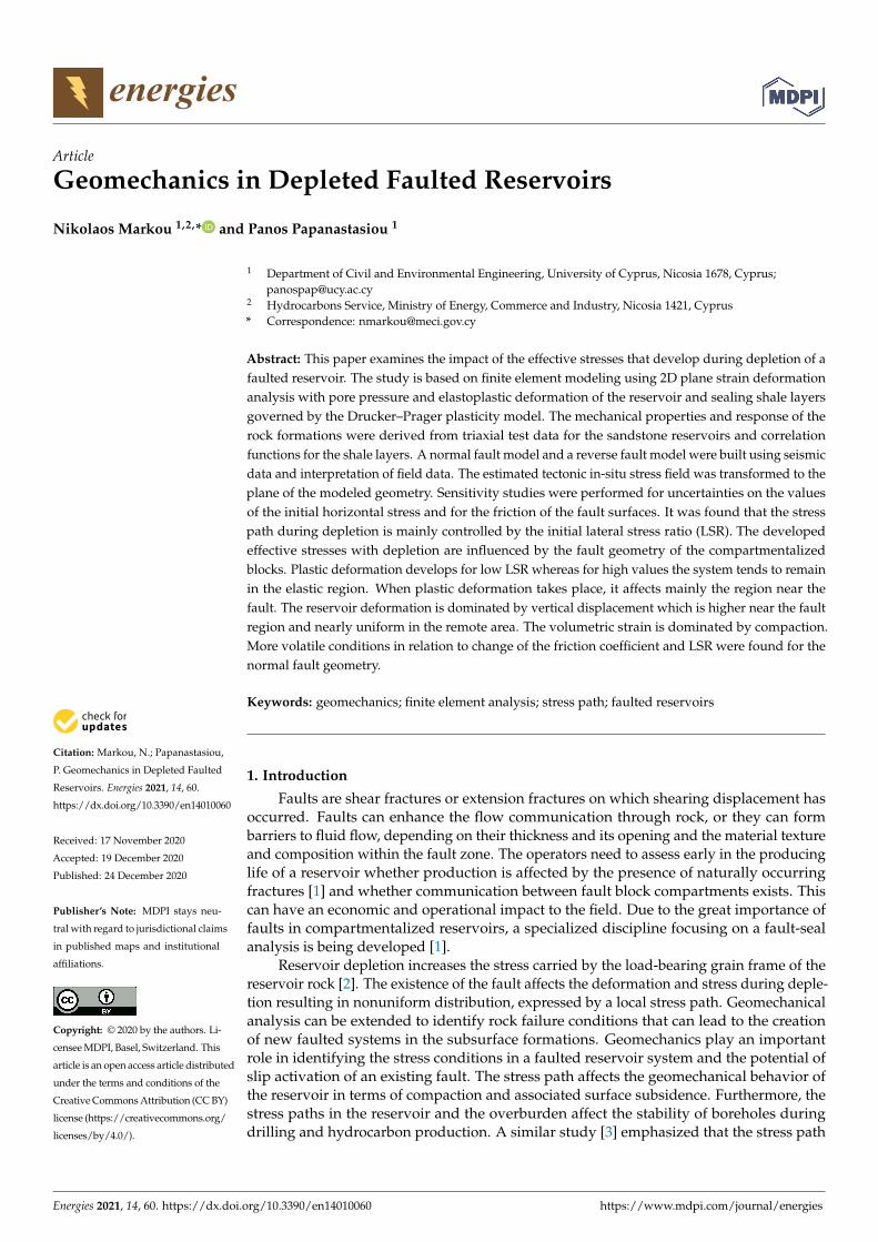
In this study the faults–joints system is simplified by considering two major faults.The geometry of the considered two faults is shown in Figure 1 where the seismic profilesare illustrated for (a) the normal fault in NW–SE section and (b) the reverse fault in SW–NEsection. The reservoir zone is illustrated within the yellow marked horizons and the faultgeometry is shown by black lines. Faults are generally not straight uniform surfaces andcommonly range from planar to listric or curved geometries, or conjugate faults. In thiscase study, shales encase the sandstone reservoir. The reservoir consists of sandstonesinterbedded by shales but in the modeling is simplified to a uniform zone.

Energies 2021, 14, 60 3 of 17Energies 2021, 14, x FOR PEER REVIEW 3 of 17

Figure 1. Seismic profile of the examined fault geometries shown by black lines (a) normal fault and (b) reverse fault. The Miocene-Oligocene interbedded sandstones are illustrated in yellow marked horizons and encased by shales.

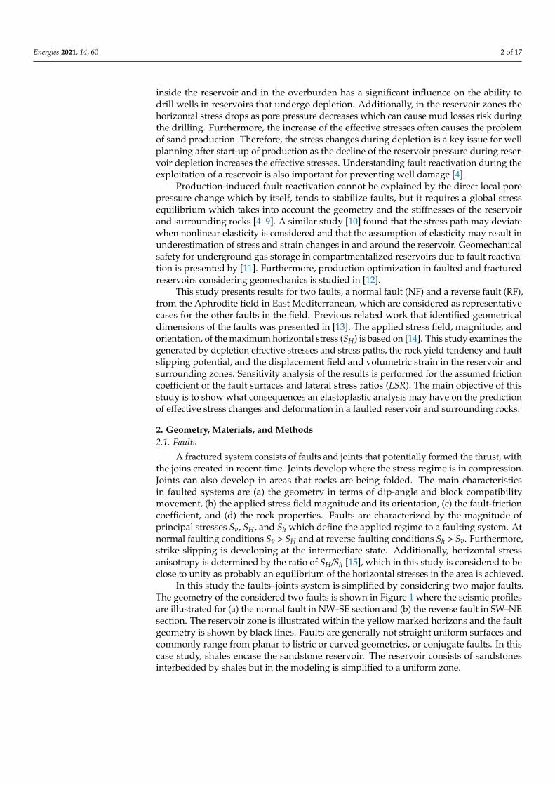
The 3D sketch of Figure 2 shows the representative volume which defines the fault contacts between the blocks. The face normal to SH corresponds to the normal fault shown in Figure 1a and the face normal to Sh corresponds to reverse fault of Figure 1b. From the geological understanding, one can assume that the reverse fault developed first followed by the formation of compressional fractures which formed the normal fault perpendicular to the reserve fault plane. Currently, the field stress is recognized to be at normal fault conditions (SH < Sv), that it had passed from the intermediate strike-slip state (SH > Sv).

Figure 2. 3D schematic representation of the considered area. The normal fault (NF) section crosses the normal fault geometry and the reverse fault (RF) section crosses the reverse fault ge-ometry.

The analysis considers two simplified structural shapes that reduce the computa-tional cost and complexity without losing the qualitative characteristics of the overall pro-cess. Each structural model consists of two fault-blocks in a normal fault and reverse fault patterns. The grid dimensions have a length (x-axis) of 4000 m and a total thickness (y-axis) of 900 m. Based on the seismic data, the fault dip for normal fault geometry is 57° and for the reverse fault geometry is 66°. The fault parameters are presented in Table 1. The vertical displacement fault throw is 100 m, hence, the right-side block has been low-ered by 100 m from its original depth in the NF case and raised by 100 m in the RF case.

Figure 1. Seismic profile of the examined fault geometries shown by black lines (a) normal fault and (b) reverse fault. TheMiocene-Oligocene interbedded sandstones are illustrated in yellow marked horizons and encased by shales.

The 3D sketch of Figure 2 shows the representative volume which defines the faultcontacts between the blocks. The face normal to SH corresponds to the normal fault shownin Figure 1a and the face normal to Sh corresponds to reverse fault of Figure 1b. From thegeological understanding, one can assume that the reverse fault developed first followedby the formation of compressional fractures which formed the normal fault perpendicularto the reserve fault plane. Currently, the field stress is recognized to be at normal faultconditions (SH < Sv), that it had passed from the intermediate strike-slip state (SH > Sv).

Energies 2021, 14, x FOR PEER REVIEW 3 of 17

Figure 1. Seismic profile of the examined fault geometries shown by black lines (a) normal fault and (b) reverse fault. The Miocene-Oligocene interbedded sandstones are illustrated in yellow marked horizons and encased by shales.

The 3D sketch of Figure 2 shows the representative volume which defines the fault contacts between the blocks. The face normal to SH corresponds to the normal fault shown in Figure 1a and the face normal to Sh corresponds to reverse fault of Figure 1b. From the geological understanding, one can assume that the reverse fault developed first followed by the formation of compressional fractures which formed the normal fault perpendicular to the reserve fault plane. Currently, the field stress is recognized to be at normal fault conditions (SH < Sv), that it had passed from the intermediate strike-slip state (SH > Sv).

Figure 2. 3D schematic representation of the considered area. The normal fault (NF) section crosses the normal fault geometry and the reverse fault (RF) section crosses the reverse fault ge-ometry.

The analysis considers two simplified structural shapes that reduce the computa-tional cost and complexity without losing the qualitative characteristics of the overall pro-cess. Each structural model consists of two fault-blocks in a normal fault and reverse fault patterns. The grid dimensions have a length (x-axis) of 4000 m and a total thickness (y-axis) of 900 m. Based on the seismic data, the fault dip for normal fault geometry is 57° and for the reverse fault geometry is 66°. The fault parameters are presented in Table 1. The vertical displacement fault throw is 100 m, hence, the right-side block has been low-ered by 100 m from its original depth in the NF case and raised by 100 m in the RF case.

Figure 2. 3D schematic representation of the considered area. The normal fault (NF) section crossesthe normal fault geometry and the reverse fault (RF) section crosses the reverse fault geometry.

The analysis considers two simplified structural shapes that reduce the computationalcost and complexity without losing the qualitative characteristics of the overall process.Each structural model consists of two fault-blocks in a normal fault and reverse faultpatterns. The grid dimensions have a length (x-axis) of 4000 m and a total thickness (y-axis)of 900 m. Based on the seismic data, the fault dip for normal fault geometry is 57◦ andfor the reverse fault geometry is 66◦. The fault parameters are presented in Table 1. Thevertical displacement fault throw is 100 m, hence, the right-side block has been loweredby 100 m from its original depth in the NF case and raised by 100 m in the RF case. Thetop of the upper grid surface is at the depth of 4800 m and the top reservoir is at 5100 m.The sealing layers amount of to two shale bodies enclosing the sandstone reservoir. The

Energies 2021, 14, 60 4 of 17

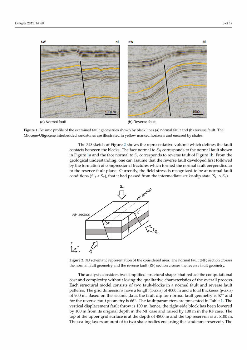
applied loads and boundary conditions in each model geometry are illustrated in Figure 3.The boundaries conditions include vertical rolling for the sides and horizontal rolling forthe base of the model. The fault blocks are connected with frictional contact surfaces. Thevertical stress, σ1 is applied as an input on the top of the model along the vertical z-axis.The selected sampling locations are carried out at defined pseudo wells and at the faultslip surface as depicted in Figure 3.

Table 1. Geometrical parameters of the examined faults based on Markou and Papanastasiou [13].

Parameter Normal Fault Reverse Fault

Dip 57◦ 66◦

Strike azimuth angle relative to North 317◦ 44◦

Transformation angle relative to SH 42◦ clockwise 51◦ clockwise

Energies 2021, 14, x FOR PEER REVIEW 4 of 17

The top of the upper grid surface is at the depth of 4800 m and the top reservoir is at 5100 m. The sealing layers amount of to two shale bodies enclosing the sandstone reservoir. The applied loads and boundary conditions in each model geometry are illustrated in Fig-ure 3. The boundaries conditions include vertical rolling for the sides and horizontal roll-ing for the base of the model. The fault blocks are connected with frictional contact sur-faces. The vertical stress, σ1 is applied as an input on the top of the model along the vertical z-axis. The selected sampling locations are carried out at defined pseudo wells and at the fault slip surface as depicted in Figure 3.

Table 1. Geometrical parameters of the examined faults based on Markou and Papanastasiou [13].

Parameter Normal Fault Reverse Fault Dip 57° 66°

Strike azimuth angle relative to North 317° 44° Transformation angle relative to SH 42° clockwise 51° clockwise

Pore pressure elements are considered at the given pressure conditions in each de-pletion scenario. The main assumption is that the formation bodies are in pressure equi-librium in each fault block. For simplifying the current process, the applied pore pressure is controlled as an input in each fault block. The model is based on the Terzaghi effective stress relation for the pore pressure and stresses.

Figure 3. Geometry of the 2D fault models. Normal fault model on the left and reverse fault model on the right.

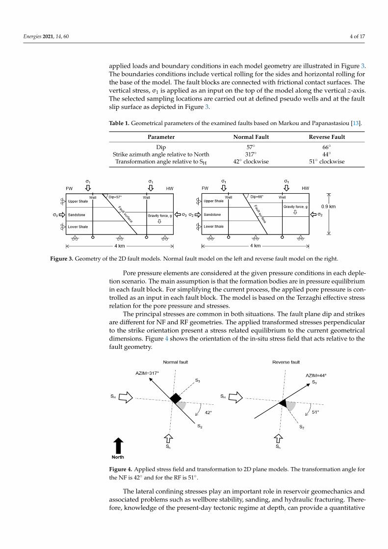
The principal stresses are common in both situations. The fault plane dip and strikes are different for NF and RF geometries. The applied transformed stresses perpendicular to the strike orientation present a stress related equilibrium to the current geometrical dimensions. Figure 4 shows the orientation of the in-situ stress field that acts relative to the fault geometry.

The lateral confining stresses play an important role in reservoir geomechanics and associated problems such as wellbore stability, sanding, and hydraulic fracturing. There-fore, knowledge of the present-day tectonic regime at depth, can provide a quantitative assessment of the horizontal stress magnitude. A first estimate of the horizontal stresses can be obtained assuming a uniaxial compression during deposition according to the the-ory of elasticity. In this case the ratio of the horizontal effective stresses to the vertical effective stress is expressed by Ko, as a function of the Poisson ratio ν [16],

퐾표 =푣

1 − 푣 (1)

Other horizontal stress values can be defined by assuming a direct value for Ko or by Ko provided by other theories and assumptions, such as plasticity and limit equilibrium according to Jacky equation [17],

퐾표 = 1 − sin휑 (2)

Figure 3. Geometry of the 2D fault models. Normal fault model on the left and reverse fault model on the right.

Pore pressure elements are considered at the given pressure conditions in each deple-tion scenario. The main assumption is that the formation bodies are in pressure equilibriumin each fault block. For simplifying the current process, the applied pore pressure is con-trolled as an input in each fault block. The model is based on the Terzaghi effective stressrelation for the pore pressure and stresses.

The principal stresses are common in both situations. The fault plane dip and strikesare different for NF and RF geometries. The applied transformed stresses perpendicularto the strike orientation present a stress related equilibrium to the current geometricaldimensions. Figure 4 shows the orientation of the in-situ stress field that acts relative to thefault geometry.

Energies 2021, 14, x FOR PEER REVIEW 5 of 17

where φ is the effective internal friction angle. Alternatively, excess horizontal stresses can be obtained by simulating the tectonic movement in FE analysis [18]. In this study, Ko is further defined in terms of changes of the effective stresses and presented in the stress path section.

Figure 4. Applied stress field and transformation to 2D plane models. The transformation angle for the NF is 42° and for the RF is 51°.

Due to the uncertainty in the magnitude of the minimum horizontal stress a sensitiv-ity analysis will be carried out for three different values of the lateral stress ratio (LSR) which is defined as the ratio of the total horizontal stress to the total vertical stress, LSR = SH/Sv. The base case scenario is the most likely one. In this case, the in-situ stresses are inserted directly in the model as residual stresses. Additional uncertainty on the results arises from the value of the friction coefficient of the fault surfaces. All the examined sce-narios are shown in Table 2.

Table 2. Scenarios for LSR and fault friction angle sensitivities.

LSR Scenarios Low Mid High S3 (MPa) 67.3 74.4 88.6

LSR 0.76 0.84 1.0 Friction Scenarios Low Mid High

Coefficient of Friction, μ 0.36 0.58 0.75 Common parameters at the center of the reservoir in all scenarios include the vertical stress, Sv =

88.6 MPa and in-situ pore pressure, Pp = 61.1 MPa. At the depletion conditions pore pressure de-creases to 40 MPa.

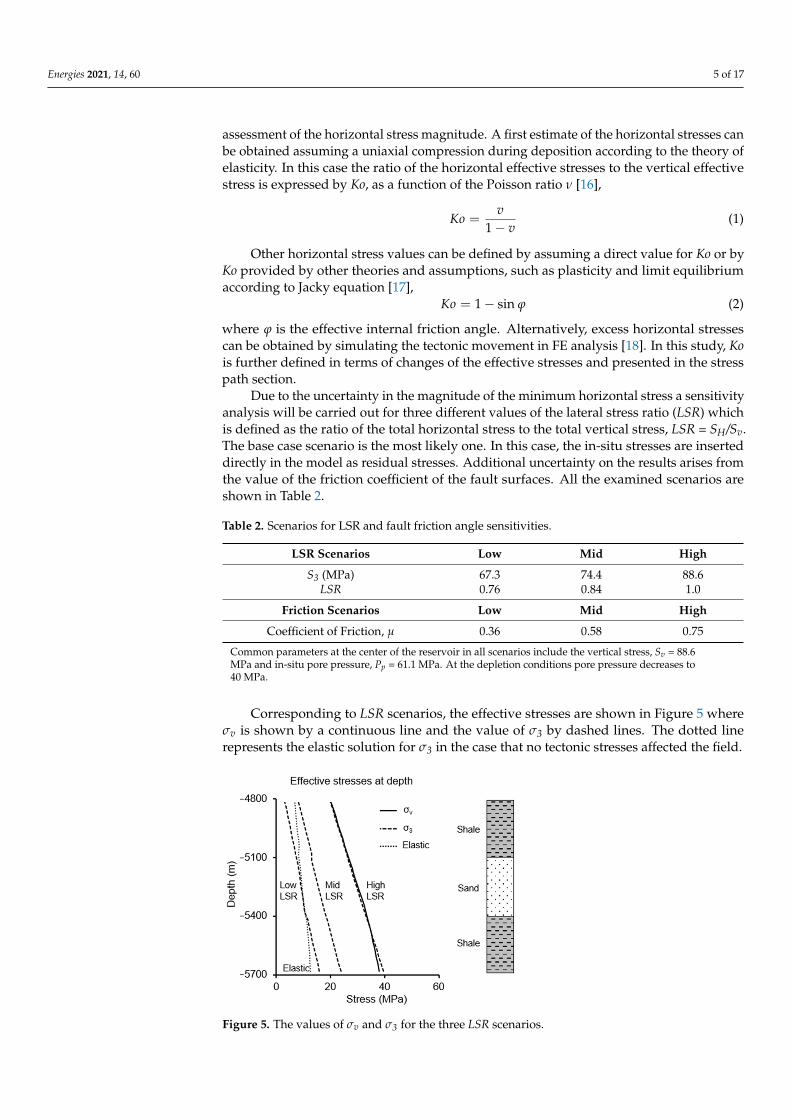
Corresponding to LSR scenarios, the effective stresses are shown in Figure 5 where σv is shown by a continuous line and the value of σ3 by dashed lines. The dotted line rep-resents the elastic solution for σ3 in the case that no tectonic stresses affected the field.

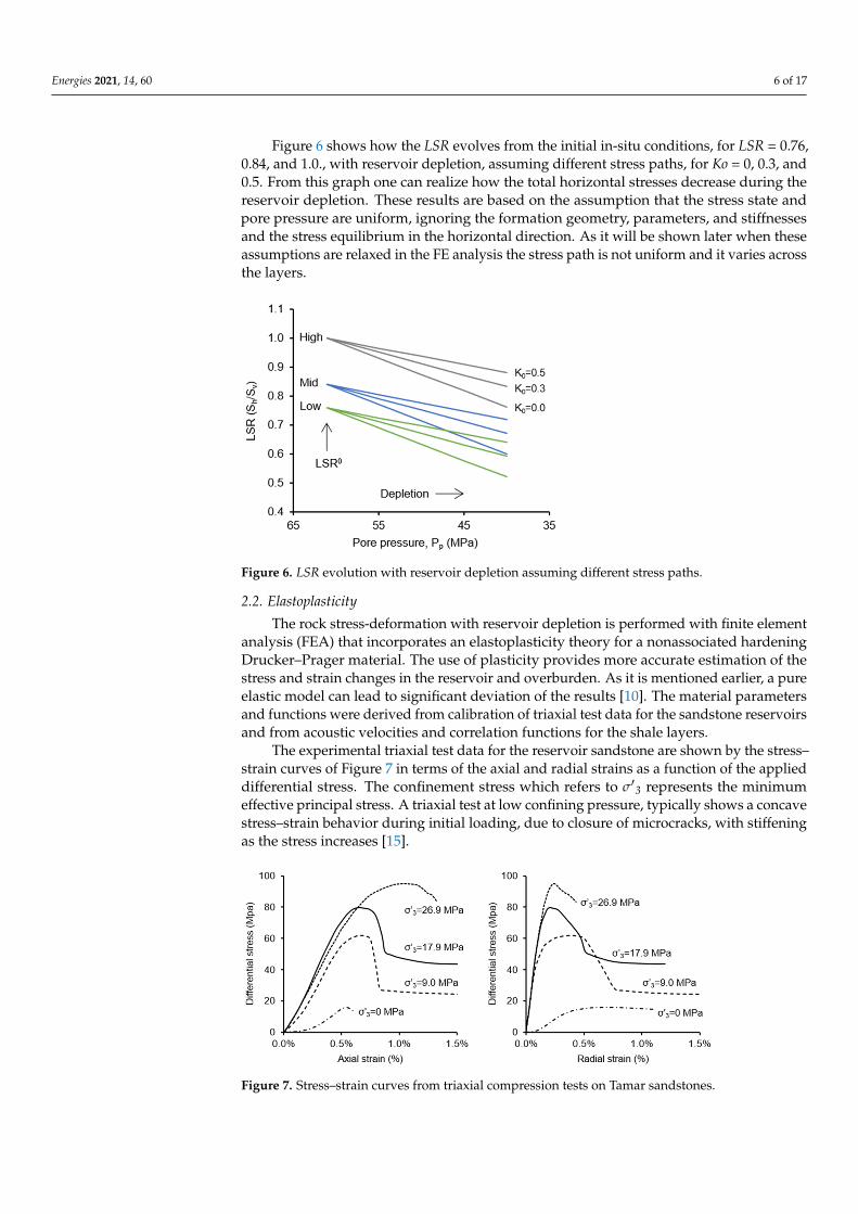
Figure 6 shows how the LSR evolves from the initial in-situ conditions, for LSR = 0.76, 0.84, and 1.0., with reservoir depletion, assuming different stress paths, for Ko = 0, 0.3, and 0.5. From this graph one can realize how the total horizontal stresses decrease during the reservoir depletion. These results are based on the assumption that the stress state and pore pressure are uniform, ignoring the formation geometry, parameters, and stiffnesses and the stress equilibrium in the horizontal direction. As it will be shown later when these assumptions are relaxed in the FE analysis the stress path is not uniform and it varies across the layers.

Figure 4. Applied stress field and transformation to 2D plane models. The transformation angle forthe NF is 42◦ and for the RF is 51◦.

The lateral confining stresses play an important role in reservoir geomechanics andassociated problems such as wellbore stability, sanding, and hydraulic fracturing. There-fore, knowledge of the present-day tectonic regime at depth, can provide a quantitative

Energies 2021, 14, 60 5 of 17

assessment of the horizontal stress magnitude. A first estimate of the horizontal stresses canbe obtained assuming a uniaxial compression during deposition according to the theory ofelasticity. In this case the ratio of the horizontal effective stresses to the vertical effectivestress is expressed by Ko, as a function of the Poisson ratio ν [16],

Ko =v

1− v(1)

Other horizontal stress values can be defined by assuming a direct value for Ko or byKo provided by other theories and assumptions, such as plasticity and limit equilibriumaccording to Jacky equation [17],

Ko = 1− sin ϕ (2)

where ϕ is the effective internal friction angle. Alternatively, excess horizontal stressescan be obtained by simulating the tectonic movement in FE analysis [18]. In this study, Kois further defined in terms of changes of the effective stresses and presented in the stresspath section.

Due to the uncertainty in the magnitude of the minimum horizontal stress a sensitivityanalysis will be carried out for three different values of the lateral stress ratio (LSR) whichis defined as the ratio of the total horizontal stress to the total vertical stress, LSR = SH/Sv.The base case scenario is the most likely one. In this case, the in-situ stresses are inserteddirectly in the model as residual stresses. Additional uncertainty on the results arises fromthe value of the friction coefficient of the fault surfaces. All the examined scenarios areshown in Table 2.

Table 2. Scenarios for LSR and fault friction angle sensitivities.

LSR Scenarios Low Mid High

S3 (MPa) 67.3 74.4 88.6LSR 0.76 0.84 1.0

Friction Scenarios Low Mid High

Coefficient of Friction, µ 0.36 0.58 0.75

Common parameters at the center of the reservoir in all scenarios include the vertical stress, Sv = 88.6MPa and in-situ pore pressure, Pp = 61.1 MPa. At the depletion conditions pore pressure decreases to40 MPa.

Corresponding to LSR scenarios, the effective stresses are shown in Figure 5 whereσv is shown by a continuous line and the value of σ3 by dashed lines. The dotted linerepresents the elastic solution for σ3 in the case that no tectonic stresses affected the field.

Energies 2021, 14, x FOR PEER REVIEW 6 of 17

Figure 5. The values of σv and σ3 for the three LSR scenarios.

Figure 6. LSR evolution with reservoir depletion assuming different stress paths.

2.2. Elastoplasticity The rock stress-deformation with reservoir depletion is performed with finite ele-

ment analysis (FEA) that incorporates an elastoplasticity theory for a nonassociated hard-ening Drucker–Prager material. The use of plasticity provides more accurate estimation of the stress and strain changes in the reservoir and overburden. As it is mentioned earlier, a pure elastic model can lead to significant deviation of the results [10]. The material pa-rameters and functions were derived from calibration of triaxial test data for the sandstone reservoirs and from acoustic velocities and correlation functions for the shale layers.

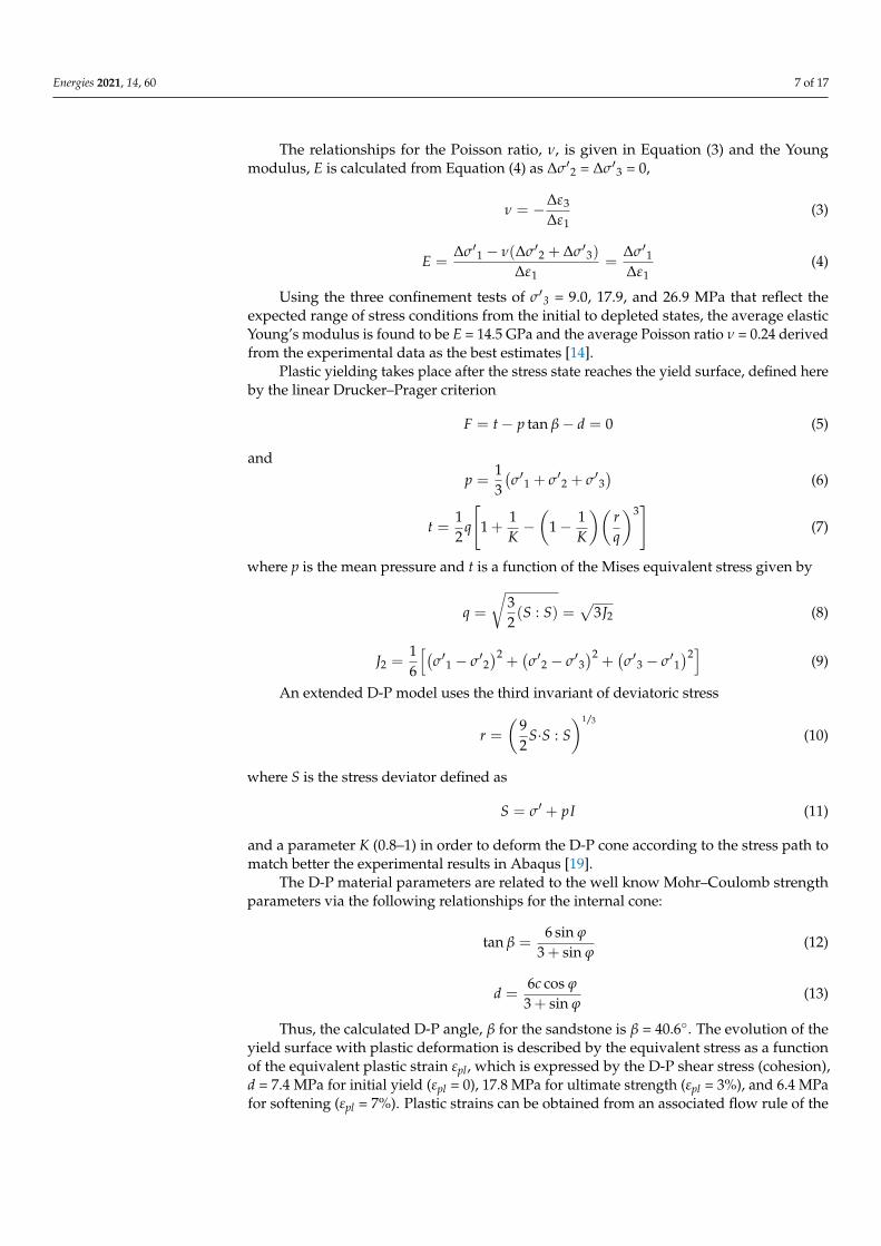
The experimental triaxial test data for the reservoir sandstone are shown by the stress–strain curves of Figure 7 in terms of the axial and radial strains as a function of the applied differential stress. The confinement stress which refers to σ′3 represents the mini-mum effective principal stress. A triaxial test at low confining pressure, typically shows a concave stress–strain behavior during initial loading, due to closure of microcracks, with stiffening as the stress increases [15].

The relationships for the Poisson ratio, ν, is given in Equation (3) and the Young mod-ulus, E is calculated from Equation (4) as Δσ′2 = Δσ′3 = 0,

휈 = −훥휀훥휀

(3)

퐸 =훥휎′ − 휈(훥휎′ + 훥휎′ )

훥휀=

훥휎′훥휀

(4)

Figure 5. The values of σv and σ3 for the three LSR scenarios.

Energies 2021, 14, 60 6 of 17

Figure 6 shows how the LSR evolves from the initial in-situ conditions, for LSR = 0.76,0.84, and 1.0., with reservoir depletion, assuming different stress paths, for Ko = 0, 0.3, and0.5. From this graph one can realize how the total horizontal stresses decrease during thereservoir depletion. These results are based on the assumption that the stress state andpore pressure are uniform, ignoring the formation geometry, parameters, and stiffnessesand the stress equilibrium in the horizontal direction. As it will be shown later when theseassumptions are relaxed in the FE analysis the stress path is not uniform and it varies acrossthe layers.

Energies 2021, 14, x FOR PEER REVIEW 6 of 17

Figure 5. The values of σv and σ3 for the three LSR scenarios.

Figure 6. LSR evolution with reservoir depletion assuming different stress paths.

2.2. Elastoplasticity The rock stress-deformation with reservoir depletion is performed with finite ele-

ment analysis (FEA) that incorporates an elastoplasticity theory for a nonassociated hard-ening Drucker–Prager material. The use of plasticity provides more accurate estimation of the stress and strain changes in the reservoir and overburden. As it is mentioned earlier, a pure elastic model can lead to significant deviation of the results [10]. The material pa-rameters and functions were derived from calibration of triaxial test data for the sandstone reservoirs and from acoustic velocities and correlation functions for the shale layers.

The experimental triaxial test data for the reservoir sandstone are shown by the stress–strain curves of Figure 7 in terms of the axial and radial strains as a function of the applied differential stress. The confinement stress which refers to σ′3 represents the mini-mum effective principal stress. A triaxial test at low confining pressure, typically shows a concave stress–strain behavior during initial loading, due to closure of microcracks, with stiffening as the stress increases [15].

The relationships for the Poisson ratio, ν, is given in Equation (3) and the Young mod-ulus, E is calculated from Equation (4) as Δσ′2 = Δσ′3 = 0,

휈 = −훥휀훥휀

(3)

퐸 =훥휎′ − 휈(훥휎′ + 훥휎′ )

훥휀=

훥휎′훥휀

(4)

Figure 6. LSR evolution with reservoir depletion assuming different stress paths.

2.2. Elastoplasticity

The rock stress-deformation with reservoir depletion is performed with finite elementanalysis (FEA) that incorporates an elastoplasticity theory for a nonassociated hardeningDrucker–Prager material. The use of plasticity provides more accurate estimation of thestress and strain changes in the reservoir and overburden. As it is mentioned earlier, a pureelastic model can lead to significant deviation of the results [10]. The material parametersand functions were derived from calibration of triaxial test data for the sandstone reservoirsand from acoustic velocities and correlation functions for the shale layers.

The experimental triaxial test data for the reservoir sandstone are shown by the stress–strain curves of Figure 7 in terms of the axial and radial strains as a function of the applieddifferential stress. The confinement stress which refers to σ′3 represents the minimumeffective principal stress. A triaxial test at low confining pressure, typically shows a concavestress–strain behavior during initial loading, due to closure of microcracks, with stiffeningas the stress increases [15].

Energies 2021, 14, x FOR PEER REVIEW 7 of 17

Using the three confinement tests of σ′3 = 9.0, 17.9, and 26.9 MPa that reflect the ex-pected range of stress conditions from the initial to depleted states, the average elastic Young’s modulus is found to be E = 14.5 GPa and the average Poisson ratio ν = 0.24 derived from the experimental data as the best estimates [14].

Figure 7. Stress–strain curves from triaxial compression tests on Tamar sandstones.

Plastic yielding takes place after the stress state reaches the yield surface, defined here by the linear Drucker–Prager criterion

퐹 = 푡 − 푝 tan 훽 − 푑 = 0 (5)

and

푝 =13

(휎′ + 휎′ + 휎′ ) (6)

푡 =12

푞 1 +1퐾

− 1 −1퐾

푟푞

(7)

where p is the mean pressure and t is a function of the Mises equivalent stress given by

푞 =32

(푆: 푆) = 3퐽 (8)

퐽 =16

[(휎′ − 휎′ ) + (휎′ − 휎′ ) + (휎′ − 휎′ ) ] (9)

An extended D-P model uses the third invariant of deviatoric stress

푟 =92

푆 ∙ 푆: 푆 (10)

where S is the stress deviator defined as

푆 = 휎′ + 푝퐼 (11)

and a parameter K (0.8–1) in order to deform the D-P cone according to the stress path to match better the experimental results in Abaqus [19].

The D-P material parameters are related to the well know Mohr–Coulomb strength parameters via the following relationships for the internal cone:

tan 훽 =6 sin 휑

3 + sin 휑 (12)

푑 =6푐 cos 휑3 + sin 휑

(13)

Figure 7. Stress–strain curves from triaxial compression tests on Tamar sandstones.

Energies 2021, 14, 60 7 of 17

The relationships for the Poisson ratio, ν, is given in Equation (3) and the Youngmodulus, E is calculated from Equation (4) as ∆σ′2 = ∆σ′3 = 0,

ν = −∆ε3

∆ε1(3)

E =∆σ′1 − ν(∆σ′2 + ∆σ′3)

∆ε1=

∆σ′1∆ε1

(4)

Using the three confinement tests of σ′3 = 9.0, 17.9, and 26.9 MPa that reflect theexpected range of stress conditions from the initial to depleted states, the average elasticYoung’s modulus is found to be E = 14.5 GPa and the average Poisson ratio ν = 0.24 derivedfrom the experimental data as the best estimates [14].

Plastic yielding takes place after the stress state reaches the yield surface, defined hereby the linear Drucker–Prager criterion

F = t− p tan β− d = 0 (5)

andp =

13(σ′1 + σ′2 + σ′3

)(6)

t =12

q

[1 +

1K−(

1− 1K

)(rq

)3]

(7)

where p is the mean pressure and t is a function of the Mises equivalent stress given by

q =

√32(S : S) =

√3J2 (8)

J2 =16

[(σ′1 − σ′2

)2+(σ′2 − σ′3

)2+(σ′3 − σ′1

)2]

(9)

An extended D-P model uses the third invariant of deviatoric stress

r =(

92

S·S : S)1/3

(10)

where S is the stress deviator defined as

S = σ′ + pI (11)

and a parameter K (0.8–1) in order to deform the D-P cone according to the stress path tomatch better the experimental results in Abaqus [19].

The D-P material parameters are related to the well know Mohr–Coulomb strengthparameters via the following relationships for the internal cone:

tan β =6 sin ϕ

3 + sin ϕ(12)

d =6c cos ϕ

3 + sin ϕ(13)

Thus, the calculated D-P angle, β for the sandstone is β = 40.6◦. The evolution of theyield surface with plastic deformation is described by the equivalent stress as a functionof the equivalent plastic strain εpl, which is expressed by the D-P shear stress (cohesion),d = 7.4 MPa for initial yield (εpl = 0), 17.8 MPa for ultimate strength (εpl = 3%), and 6.4 MPafor softening (εpl = 7%). Plastic strains can be obtained from an associated flow rule of the

Energies 2021, 14, 60 8 of 17

Drucker–Prager model. When dilation, ψ = β, the model can provides unrealistic volumeincreases, so, we used a nonassociative model defined by dilation, ψ given by

tan ψ =6 sin(ϕ− 20◦)

3 + sin(ϕ− 20◦)(14)

which for the Tamar sandstone with ϕ = 30◦, results in ψ = 18.2◦.For the shale layers, the rock parameters were determined from acoustic data and

correlation functions. For the compressional velocity measurements of Vp = 3.5 km/s [15],the correlation in Equation (15) yields the uniaxial compressive strength [20].

C0 = 0.77Vp2.93 (15)

which gives C0 = 30.2 MPa. For a representative friction angle of shale, ϕ = 20◦, thecorresponding value of the cohesion c is derived from the Mohr–Coulomb relation via

c =1− sin ϕ

2 cos ϕC0 (16)

which gives c = 10.5 MPa [18]. These values correspond to the D-P material parameters β =31.6◦, d = 17.7 MPa, and ψ = 0. No plastic hardening was assumed for the shale layers. Therock properties are summarized below in Table 3.

Table 3. Rock properties of the modeled formations based on Markou and Papanastasiou [14].

Parameter Sandstone Shale

Porosity, ϕ (fraction) 0.20 0.10Young modulus, E (GPa) 14.5 41.8

Poisson’s ratio, ν 0.24 0.25Drucker–Prager angle, β (degrees) 40.6◦ 31.6◦

Peak strength, d (MPa) 17.8 17.7Dilation angle, ψ (degrees) 18.2◦ 0.0◦

3. Results

The parametric studies present results for the base case scenario which corresponds tothe most likely parameters and further sensitivity analysis for the uncertain parameters.The results are presented and compared for the two reservoir fault geometries. Reservoirdepletion was simulated by decreasing the reservoir pressure to a final equilibrium state.Results were obtained and presented for the effective stresses, volumetric strain, yieldtendency, slipping potential, and displacement field in the reservoir and surrounding zones.

3.1. Effective Stresses

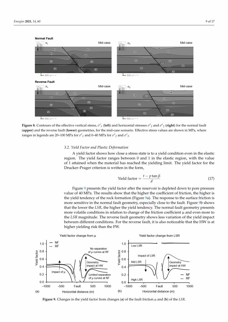
Figure 8 presents results of the mid-case scenario for the effective vertical stress, σ′vand the minimum horizontal stress, σ′3 for the normal fault and reverse fault geometriesafter reservoir depletion. These results, in comparison with the initial profile of Figure 5,show how the geometry and rock properties impact the stress distribution across the faultplane. The deviation of the stress field near the fault surfaces is clearly demonstrated bycomparing it with the far-field stresses at the remote boundaries.

Energies 2021, 14, 60 9 of 17Energies 2021, 14, x FOR PEER REVIEW 9 of 17

Figure 8. Contours of the effective vertical stress, σ′v (left) and horizontal stresses σ′3 and σ′2 (right) for the normal fault (upper) and the reverse fault (lower) geometries, for the mid-case scenario. Effective stress values are shown in MPa, where ranges in legends are 20–100 MPa for σ′v and 0–40 MPa for σ′2 and σ′3.

3.2. Yield Factor and Plastic Deformation A yield factor shows how close a stress state is to a yield condition even in the elastic

region. The yield factor ranges between 0 and 1 in the elastic region, with the value of 1 attained when the material has reached the yielding limit. The yield factor for the Drucker–Prager criterion is written in the form,

Yield factor =푡 − 푝 tan 훽

푑 (17)

Figure 9 presents the yield factor after the reservoir is depleted down to pore pressure value of 40 MPa. The results show that the higher the coefficient of friction, the higher is the yield tendency of the rock formation (Figure 9a). The response to the surface friction is more sensitive in the normal fault geometry, especially close to the fault. Figure 9b shows that the lower the LSR, the higher the yield tendency. The normal fault geometry presents more volatile conditions in relation to change of the friction coefficient μ and even more to the LSR magnitude. The reverse fault geometry shows less variation of the yield impact between different conditions. For the reverse fault, it is also noticeable that the HW is at higher yielding risk than the FW.

Figure 8. Contours of the effective vertical stress, σ′v (left) and horizontal stresses σ′3 and σ′2 (right) for the normal fault(upper) and the reverse fault (lower) geometries, for the mid-case scenario. Effective stress values are shown in MPa, whereranges in legends are 20–100 MPa for σ′v and 0–40 MPa for σ′2 and σ′3.

3.2. Yield Factor and Plastic Deformation

A yield factor shows how close a stress state is to a yield condition even in the elasticregion. The yield factor ranges between 0 and 1 in the elastic region, with the valueof 1 attained when the material has reached the yielding limit. The yield factor for theDrucker–Prager criterion is written in the form,

Yield factor =t− p tan β

d(17)

Figure 9 presents the yield factor after the reservoir is depleted down to pore pressurevalue of 40 MPa. The results show that the higher the coefficient of friction, the higher isthe yield tendency of the rock formation (Figure 9a). The response to the surface friction ismore sensitive in the normal fault geometry, especially close to the fault. Figure 9b showsthat the lower the LSR, the higher the yield tendency. The normal fault geometry presentsmore volatile conditions in relation to change of the friction coefficient µ and even more tothe LSR magnitude. The reverse fault geometry shows less variation of the yield impactbetween different conditions. For the reverse fault, it is also noticeable that the HW is athigher yielding risk than the FW.

Energies 2021, 14, x FOR PEER REVIEW 9 of 17

Figure 8. Contours of the effective vertical stress, σ′v (left) and horizontal stresses σ′3 and σ′2 (right) for the normal fault (upper) and the reverse fault (lower) geometries, for the mid-case scenario. Effective stress values are shown in MPa, where ranges in legends are 20–100 MPa for σ′v and 0–40 MPa for σ′2 and σ′3.

3.2. Yield Factor and Plastic Deformation A yield factor shows how close a stress state is to a yield condition even in the elastic

region. The yield factor ranges between 0 and 1 in the elastic region, with the value of 1 attained when the material has reached the yielding limit. The yield factor for the Drucker–Prager criterion is written in the form,

Yield factor =푡 − 푝 tan 훽

푑 (17)

Figure 9 presents the yield factor after the reservoir is depleted down to pore pressure value of 40 MPa. The results show that the higher the coefficient of friction, the higher is the yield tendency of the rock formation (Figure 9a). The response to the surface friction is more sensitive in the normal fault geometry, especially close to the fault. Figure 9b shows that the lower the LSR, the higher the yield tendency. The normal fault geometry presents more volatile conditions in relation to change of the friction coefficient μ and even more to the LSR magnitude. The reverse fault geometry shows less variation of the yield impact between different conditions. For the reverse fault, it is also noticeable that the HW is at higher yielding risk than the FW.

Figure 9. Changes in the yield factor from changes (a) of the fault friction µ and (b) of the LSR.

Energies 2021, 14, 60 10 of 17

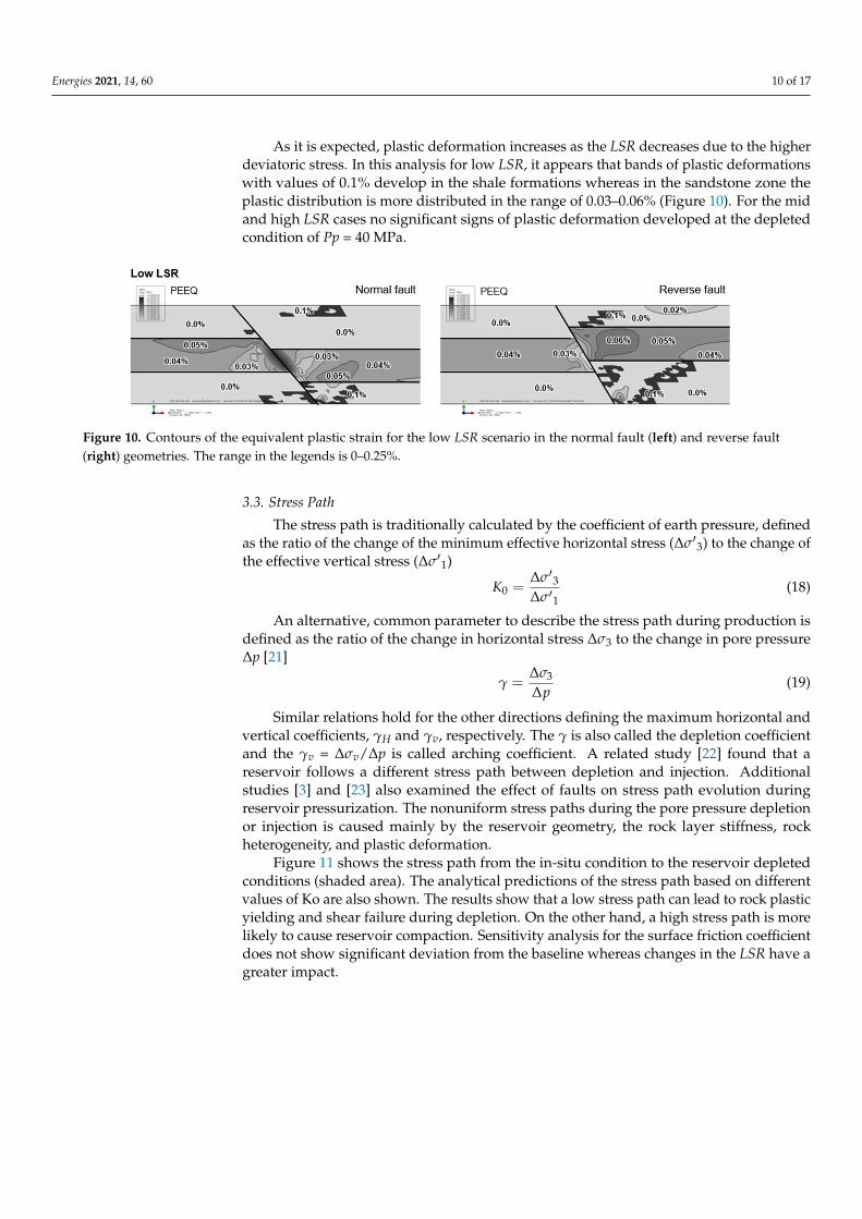
As it is expected, plastic deformation increases as the LSR decreases due to the higherdeviatoric stress. In this analysis for low LSR, it appears that bands of plastic deformationswith values of 0.1% develop in the shale formations whereas in the sandstone zone theplastic distribution is more distributed in the range of 0.03–0.06% (Figure 10). For the midand high LSR cases no significant signs of plastic deformation developed at the depletedcondition of Pp = 40 MPa.

Energies 2021, 14, x FOR PEER REVIEW 10 of 17

Figure 9. Changes in the yield factor from changes (a) of the fault friction μ and (b) of the LSR.

As it is expected, plastic deformation increases as the LSR decreases due to the higher deviatoric stress. In this analysis for low LSR, it appears that bands of plastic deformations with values of 0.1% develop in the shale formations whereas in the sandstone zone the plastic distribution is more distributed in the range of 0.03–0.06% (Figure 10). For the mid and high LSR cases no significant signs of plastic deformation developed at the depleted condition of Pp = 40 MPa.

Figure 10. Contours of the equivalent plastic strain for the low LSR scenario in the normal fault (left) and reverse fault (right) geometries. The range in the legends is 0–0.25%.

3.3. Stress Path The stress path is traditionally calculated by the coefficient of earth pressure, defined

as the ratio of the change of the minimum effective horizontal stress (Δσ′3) to the change of the effective vertical stress (Δσ′1)

퐾 =∆휎′∆휎′

(18)

An alternative, common parameter to describe the stress path during production is defined as the ratio of the change in horizontal stress Δσ3 to the change in pore pressure Δp [21]

훾 =∆휎∆푝

(19)

Similar relations hold for the other directions defining the maximum horizontal and vertical coefficients, γH and γv, respectively. The γ is also called the depletion coefficient and the γv = Δσv/Δp is called arching coefficient. A related study [22] found that a reservoir follows a different stress path between depletion and injection. Additional studies [3] and [23] also examined the effect of faults on stress path evolution during reservoir pressuri-zation. The nonuniform stress paths during the pore pressure depletion or injection is caused mainly by the reservoir geometry, the rock layer stiffness, rock heterogeneity, and plastic deformation.

Figure 11 shows the stress path from the in-situ condition to the reservoir depleted conditions (shaded area). The analytical predictions of the stress path based on different values of Ko are also shown. The results show that a low stress path can lead to rock plastic yielding and shear failure during depletion. On the other hand, a high stress path is more likely to cause reservoir compaction. Sensitivity analysis for the surface friction coefficient does not show significant deviation from the baseline whereas changes in the LSR have a greater impact.

Figure 10. Contours of the equivalent plastic strain for the low LSR scenario in the normal fault (left) and reverse fault(right) geometries. The range in the legends is 0–0.25%.

3.3. Stress Path

The stress path is traditionally calculated by the coefficient of earth pressure, definedas the ratio of the change of the minimum effective horizontal stress (∆σ′3) to the change ofthe effective vertical stress (∆σ′1)

K0 =∆σ′3∆σ′1

(18)

An alternative, common parameter to describe the stress path during production isdefined as the ratio of the change in horizontal stress ∆σ3 to the change in pore pressure∆p [21]

γ =∆σ3

∆p(19)

Similar relations hold for the other directions defining the maximum horizontal andvertical coefficients, γH and γv, respectively. The γ is also called the depletion coefficientand the γv = ∆σv/∆p is called arching coefficient. A related study [22] found that areservoir follows a different stress path between depletion and injection. Additionalstudies [3] and [23] also examined the effect of faults on stress path evolution duringreservoir pressurization. The nonuniform stress paths during the pore pressure depletionor injection is caused mainly by the reservoir geometry, the rock layer stiffness, rockheterogeneity, and plastic deformation.

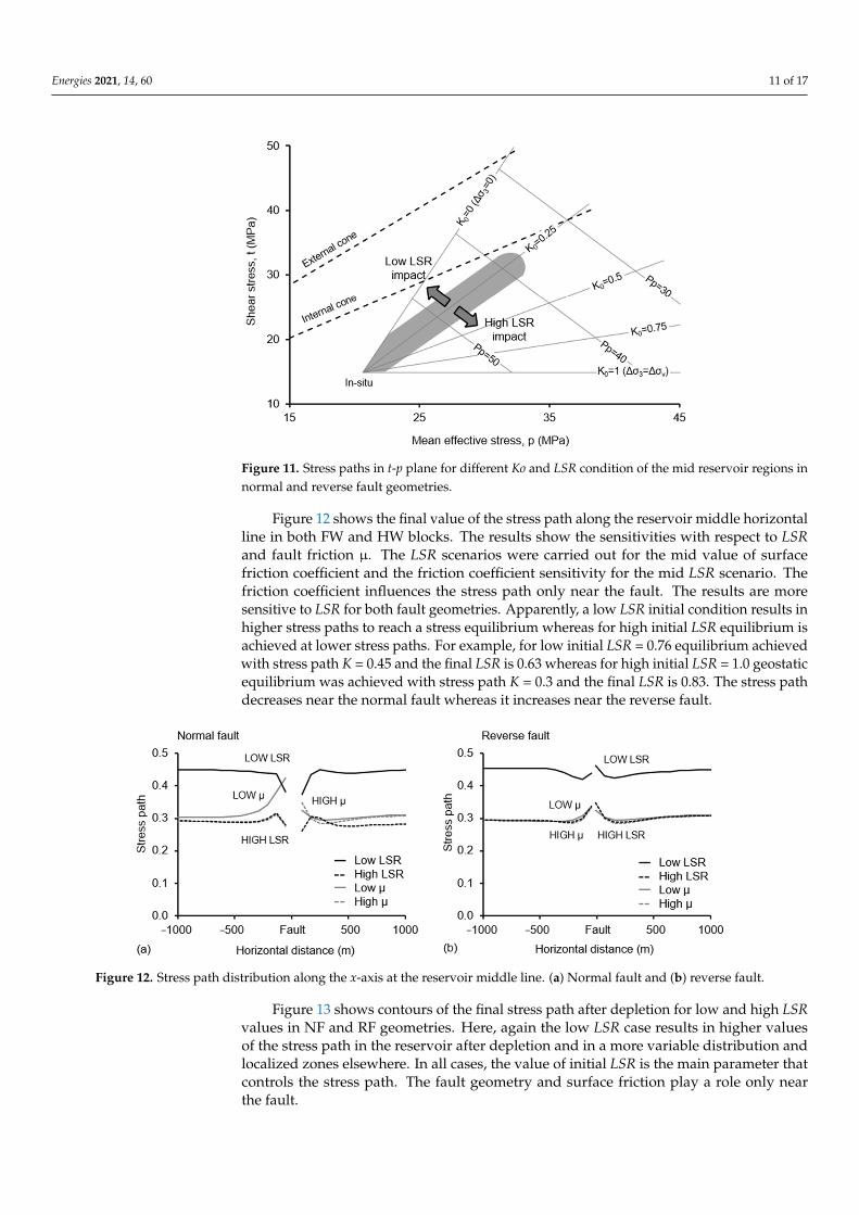
Figure 11 shows the stress path from the in-situ condition to the reservoir depletedconditions (shaded area). The analytical predictions of the stress path based on differentvalues of Ko are also shown. The results show that a low stress path can lead to rock plasticyielding and shear failure during depletion. On the other hand, a high stress path is morelikely to cause reservoir compaction. Sensitivity analysis for the surface friction coefficientdoes not show significant deviation from the baseline whereas changes in the LSR have agreater impact.

Energies 2021, 14, 60 11 of 17Energies 2021, 14, x FOR PEER REVIEW 11 of 17

Figure 11. Stress paths in t-p plane for different Ko and LSR condition of the mid reservoir regions in normal and reverse fault geometries.

Figure 12 shows the final value of the stress path along the reservoir middle horizon-tal line in both FW and HW blocks. The results show the sensitivities with respect to LSR and fault friction μ. The LSR scenarios were carried out for the mid value of surface fric-tion coefficient and the friction coefficient sensitivity for the mid LSR scenario. The friction coefficient influences the stress path only near the fault. The results are more sensitive to LSR for both fault geometries. Apparently, a low LSR initial condition results in higher stress paths to reach a stress equilibrium whereas for high initial LSR equilibrium is achieved at lower stress paths. For example, for low initial LSR = 0.76 equilibrium achieved with stress path K = 0.45 and the final LSR is 0.63 whereas for high initial LSR = 1.0 geostatic equilibrium was achieved with stress path K = 0.3 and the final LSR is 0.83. The stress path decreases near the normal fault whereas it increases near the reverse fault.

Figure 13 shows contours of the final stress path after depletion for low and high LSR values in NF and RF geometries. Here, again the low LSR case results in higher values of the stress path in the reservoir after depletion and in a more variable distribution and localized zones elsewhere. In all cases, the value of initial LSR is the main parameter that controls the stress path. The fault geometry and surface friction play a role only near the fault.

Figure 12. Stress path distribution along the x-axis at the reservoir middle line. (a) Normal fault and (b) reverse fault.

Figure 11. Stress paths in t-p plane for different Ko and LSR condition of the mid reservoir regions innormal and reverse fault geometries.

Figure 12 shows the final value of the stress path along the reservoir middle horizontalline in both FW and HW blocks. The results show the sensitivities with respect to LSRand fault friction µ. The LSR scenarios were carried out for the mid value of surfacefriction coefficient and the friction coefficient sensitivity for the mid LSR scenario. Thefriction coefficient influences the stress path only near the fault. The results are moresensitive to LSR for both fault geometries. Apparently, a low LSR initial condition results inhigher stress paths to reach a stress equilibrium whereas for high initial LSR equilibrium isachieved at lower stress paths. For example, for low initial LSR = 0.76 equilibrium achievedwith stress path K = 0.45 and the final LSR is 0.63 whereas for high initial LSR = 1.0 geostaticequilibrium was achieved with stress path K = 0.3 and the final LSR is 0.83. The stress pathdecreases near the normal fault whereas it increases near the reverse fault.

Energies 2021, 14, x FOR PEER REVIEW 11 of 17

Figure 11. Stress paths in t-p plane for different Ko and LSR condition of the mid reservoir regions in normal and reverse fault geometries.

Figure 12 shows the final value of the stress path along the reservoir middle horizon-tal line in both FW and HW blocks. The results show the sensitivities with respect to LSR and fault friction μ. The LSR scenarios were carried out for the mid value of surface fric-tion coefficient and the friction coefficient sensitivity for the mid LSR scenario. The friction coefficient influences the stress path only near the fault. The results are more sensitive to LSR for both fault geometries. Apparently, a low LSR initial condition results in higher stress paths to reach a stress equilibrium whereas for high initial LSR equilibrium is achieved at lower stress paths. For example, for low initial LSR = 0.76 equilibrium achieved with stress path K = 0.45 and the final LSR is 0.63 whereas for high initial LSR = 1.0 geostatic equilibrium was achieved with stress path K = 0.3 and the final LSR is 0.83. The stress path decreases near the normal fault whereas it increases near the reverse fault.

Figure 13 shows contours of the final stress path after depletion for low and high LSR values in NF and RF geometries. Here, again the low LSR case results in higher values of the stress path in the reservoir after depletion and in a more variable distribution and localized zones elsewhere. In all cases, the value of initial LSR is the main parameter that controls the stress path. The fault geometry and surface friction play a role only near the fault.

Figure 12. Stress path distribution along the x-axis at the reservoir middle line. (a) Normal fault and (b) reverse fault. Figure 12. Stress path distribution along the x-axis at the reservoir middle line. (a) Normal fault and (b) reverse fault.

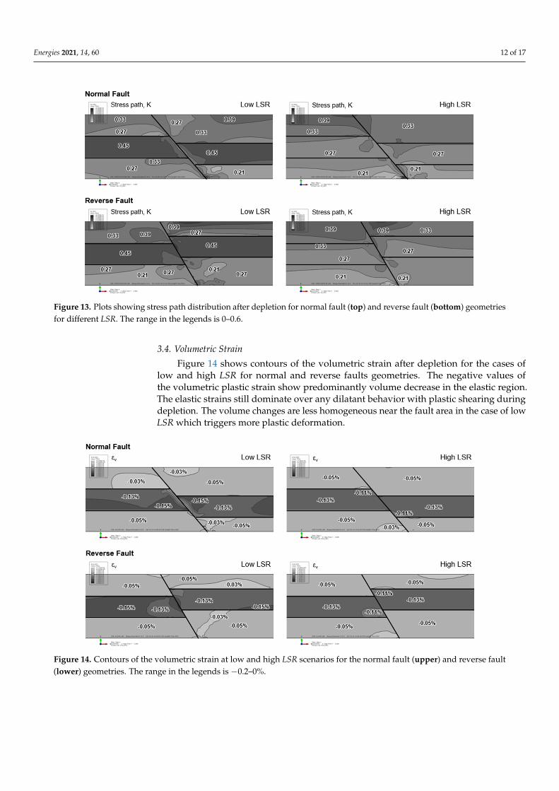
Figure 13 shows contours of the final stress path after depletion for low and high LSRvalues in NF and RF geometries. Here, again the low LSR case results in higher valuesof the stress path in the reservoir after depletion and in a more variable distribution andlocalized zones elsewhere. In all cases, the value of initial LSR is the main parameter thatcontrols the stress path. The fault geometry and surface friction play a role only nearthe fault.

Energies 2021, 14, 60 12 of 17Energies 2021, 14, x FOR PEER REVIEW 12 of 17

Figure 13. Plots showing stress path distribution after depletion for normal fault (top) and reverse fault (bottom) geome-tries for different LSR. The range in the legends is 0–0.6.

3.4. Volumetric Strain Figure 14 shows contours of the volumetric strain after depletion for the cases of low

and high LSR for normal and reverse faults geometries. The negative values of the volu-metric plastic strain show predominantly volume decrease in the elastic region. The elastic strains still dominate over any dilatant behavior with plastic shearing during depletion. The volume changes are less homogeneous near the fault area in the case of low LSR which triggers more plastic deformation.

Figure 14. Contours of the volumetric strain at low and high LSR scenarios for the normal fault (upper) and reverse fault (lower) geometries. The range in the legends is −0.2–0%.

Figure 13. Plots showing stress path distribution after depletion for normal fault (top) and reverse fault (bottom) geometriesfor different LSR. The range in the legends is 0–0.6.

3.4. Volumetric Strain

Figure 14 shows contours of the volumetric strain after depletion for the cases oflow and high LSR for normal and reverse faults geometries. The negative values ofthe volumetric plastic strain show predominantly volume decrease in the elastic region.The elastic strains still dominate over any dilatant behavior with plastic shearing duringdepletion. The volume changes are less homogeneous near the fault area in the case of lowLSR which triggers more plastic deformation.

Energies 2021, 14, x FOR PEER REVIEW 12 of 17

Figure 13. Plots showing stress path distribution after depletion for normal fault (top) and reverse fault (bottom) geome-tries for different LSR. The range in the legends is 0–0.6.

3.4. Volumetric Strain Figure 14 shows contours of the volumetric strain after depletion for the cases of low

and high LSR for normal and reverse faults geometries. The negative values of the volu-metric plastic strain show predominantly volume decrease in the elastic region. The elastic strains still dominate over any dilatant behavior with plastic shearing during depletion. The volume changes are less homogeneous near the fault area in the case of low LSR which triggers more plastic deformation.

Figure 14. Contours of the volumetric strain at low and high LSR scenarios for the normal fault (upper) and reverse fault (lower) geometries. The range in the legends is −0.2–0%.

Figure 14. Contours of the volumetric strain at low and high LSR scenarios for the normal fault (upper) and reverse fault(lower) geometries. The range in the legends is −0.2–0%.

Energies 2021, 14, 60 13 of 17

3.5. Slip Factor

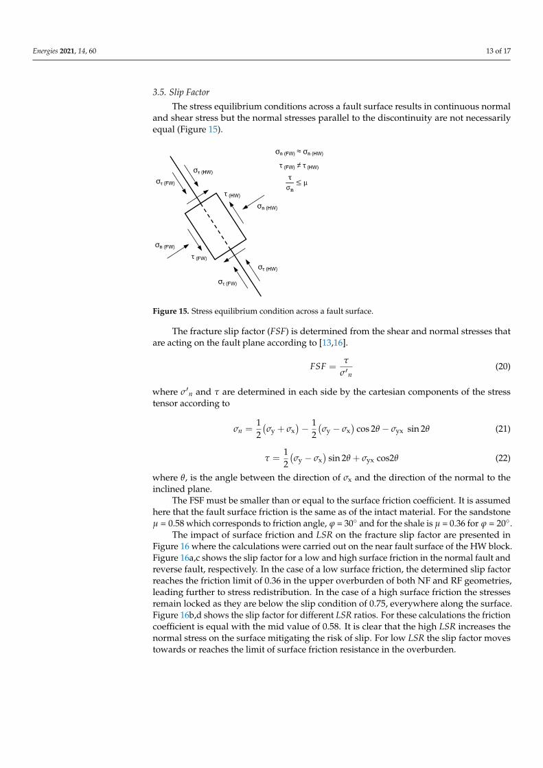
The stress equilibrium conditions across a fault surface results in continuous normaland shear stress but the normal stresses parallel to the discontinuity are not necessarilyequal (Figure 15).

Energies 2021, 14, x FOR PEER REVIEW 13 of 17

3.5. Slip Factor The stress equilibrium conditions across a fault surface results in continuous normal

and shear stress but the normal stresses parallel to the discontinuity are not necessarily equal (Figure 15).

Figure 15. Stress equilibrium condition across a fault surface.

The fracture slip factor (FSF) is determined from the shear and normal stresses that are acting on the fault plane according to [16] and [13].

퐹푆퐹 =휏

휎′ (20)

where σ′n and τ are determined in each side by the cartesian components of the stress tensor according to

휎 =12

휎 + 휎 −12

휎 − 휎 cos 2휃 − 휎 sin2휃 (21)

휏 =12

휎 − 휎 sin 2휃 + 휎 cos2휃 (22)

where θ, is the angle between the direction of 휎 and the direction of the normal to the inclined plane.

The FSF must be smaller than or equal to the surface friction coefficient. It is assumed here that the fault surface friction is the same as of the intact material. For the sandstone μ = 0.58 which corresponds to friction angle, φ = 30° and for the shale is μ = 0.36 for φ = 20°.

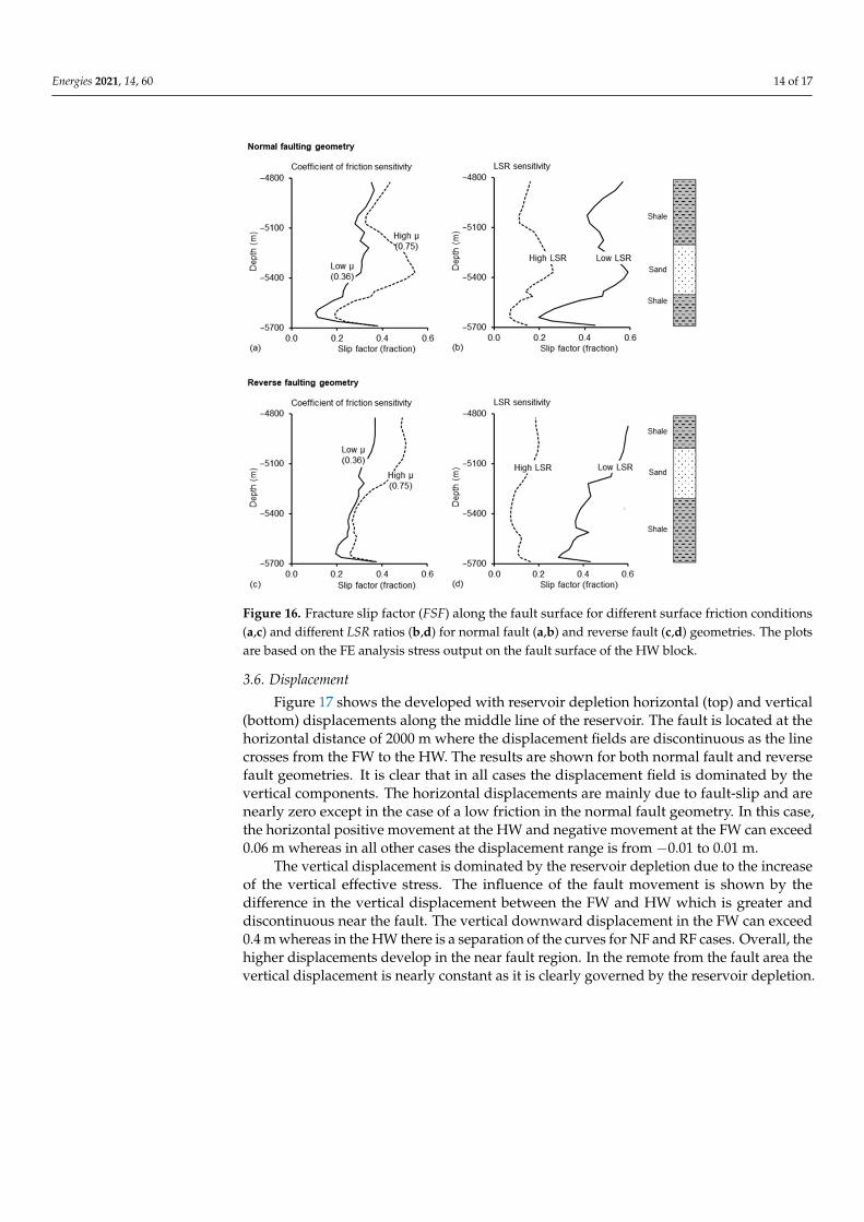
The impact of surface friction and LSR on the fracture slip factor are presented in Figure 16 where the calculations were carried out on the near fault surface of the HW block. Figure 16a,c shows the slip factor for a low and high surface friction in the normal fault and reverse fault, respectively. In the case of a low surface friction, the determined slip factor reaches the friction limit of 0.36 in the upper overburden of both NF and RF geometries, leading further to stress redistribution. In the case of a high surface friction the stresses remain locked as they are below the slip condition of 0.75, everywhere along the surface. Figure 16b,d shows the slip factor for different LSR ratios. For these calcula-tions the friction coefficient is equal with the mid value of 0.58. It is clear that the high LSR increases the normal stress on the surface mitigating the risk of slip. For low LSR the slip factor moves towards or reaches the limit of surface friction resistance in the overburden.

Figure 15. Stress equilibrium condition across a fault surface.

The fracture slip factor (FSF) is determined from the shear and normal stresses thatare acting on the fault plane according to [13,16].

FSF =τ

σ′n(20)

where σ′n and τ are determined in each side by the cartesian components of the stresstensor according to

σn =12(σy + σx

)− 1

2(σy − σx

)cos 2θ − σyx sin 2θ (21)

τ =12(σy − σx

)sin 2θ + σyx cos2θ (22)

where θ, is the angle between the direction of σx and the direction of the normal to theinclined plane.

The FSF must be smaller than or equal to the surface friction coefficient. It is assumedhere that the fault surface friction is the same as of the intact material. For the sandstoneµ = 0.58 which corresponds to friction angle, ϕ = 30◦ and for the shale is µ = 0.36 for ϕ = 20◦.

The impact of surface friction and LSR on the fracture slip factor are presented inFigure 16 where the calculations were carried out on the near fault surface of the HW block.Figure 16a,c shows the slip factor for a low and high surface friction in the normal fault andreverse fault, respectively. In the case of a low surface friction, the determined slip factorreaches the friction limit of 0.36 in the upper overburden of both NF and RF geometries,leading further to stress redistribution. In the case of a high surface friction the stressesremain locked as they are below the slip condition of 0.75, everywhere along the surface.Figure 16b,d shows the slip factor for different LSR ratios. For these calculations the frictioncoefficient is equal with the mid value of 0.58. It is clear that the high LSR increases thenormal stress on the surface mitigating the risk of slip. For low LSR the slip factor movestowards or reaches the limit of surface friction resistance in the overburden.

Energies 2021, 14, 60 14 of 17Energies 2021, 14, x FOR PEER REVIEW 14 of 17

Figure 16. Fracture slip factor (FSF) along the fault surface for different surface friction conditions (a,c) and different LSR ratios (b,d) for normal fault (a,b) and reverse fault (c,d) geometries. The plots are based on the FE analysis stress output on the fault surface of the HW block.

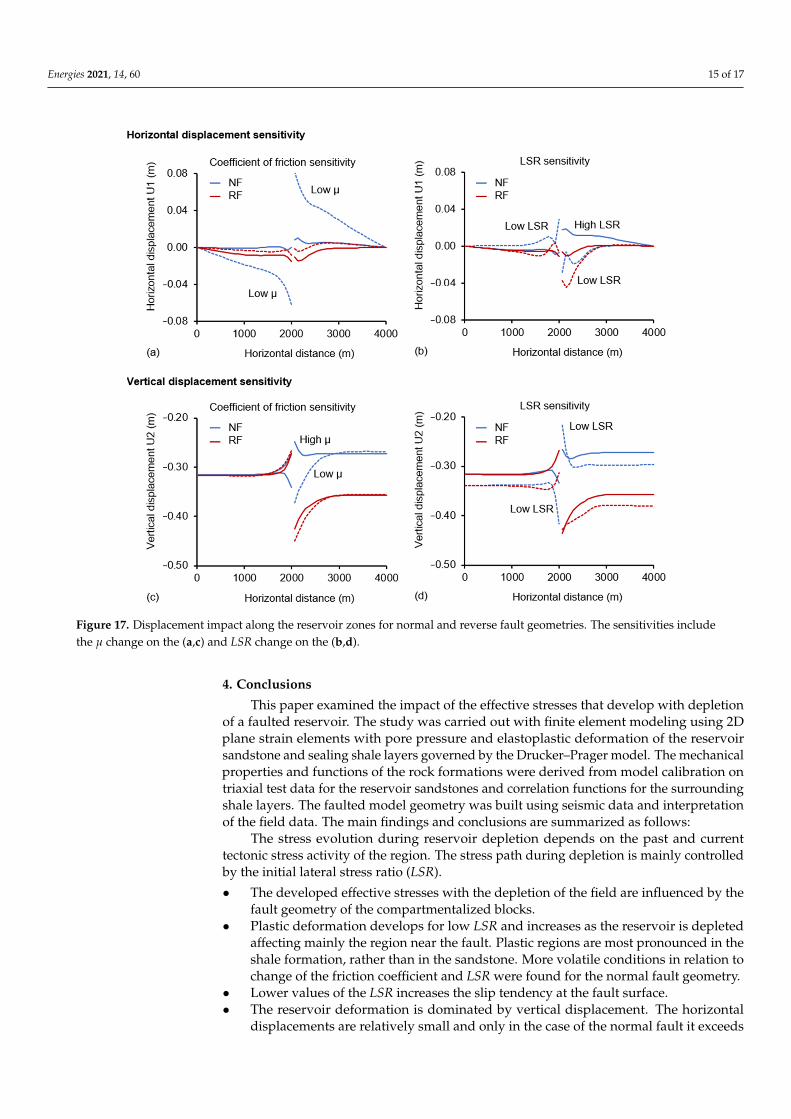
3.6. Displacement Figure 17 shows the developed with reservoir depletion horizontal (top) and vertical

(bottom) displacements along the middle line of the reservoir. The fault is located at the horizontal distance of 2000 m where the displacement fields are discontinuous as the line crosses from the FW to the HW. The results are shown for both normal fault and reverse fault geometries. It is clear that in all cases the displacement field is dominated by the vertical components. The horizontal displacements are mainly due to fault-slip and are nearly zero except in the case of a low friction in the normal fault geometry. In this case, the horizontal positive movement at the HW and negative movement at the FW can ex-ceed 0.06 m whereas in all other cases the displacement range is from −0.01 to 0.01 m.

The vertical displacement is dominated by the reservoir depletion due to the increase of the vertical effective stress. The influence of the fault movement is shown by the differ-ence in the vertical displacement between the FW and HW which is greater and discon-tinuous near the fault. The vertical downward displacement in the FW can exceed 0.4 m whereas in the HW there is a separation of the curves for NF and RF cases. Overall, the higher displacements develop in the near fault region. In the remote from the fault area the vertical displacement is nearly constant as it is clearly governed by the reservoir de-pletion.

Figure 16. Fracture slip factor (FSF) along the fault surface for different surface friction conditions(a,c) and different LSR ratios (b,d) for normal fault (a,b) and reverse fault (c,d) geometries. The plotsare based on the FE analysis stress output on the fault surface of the HW block.

3.6. Displacement

Figure 17 shows the developed with reservoir depletion horizontal (top) and vertical(bottom) displacements along the middle line of the reservoir. The fault is located at thehorizontal distance of 2000 m where the displacement fields are discontinuous as the linecrosses from the FW to the HW. The results are shown for both normal fault and reversefault geometries. It is clear that in all cases the displacement field is dominated by thevertical components. The horizontal displacements are mainly due to fault-slip and arenearly zero except in the case of a low friction in the normal fault geometry. In this case,the horizontal positive movement at the HW and negative movement at the FW can exceed0.06 m whereas in all other cases the displacement range is from −0.01 to 0.01 m.

The vertical displacement is dominated by the reservoir depletion due to the increaseof the vertical effective stress. The influence of the fault movement is shown by thedifference in the vertical displacement between the FW and HW which is greater anddiscontinuous near the fault. The vertical downward displacement in the FW can exceed0.4 m whereas in the HW there is a separation of the curves for NF and RF cases. Overall, thehigher displacements develop in the near fault region. In the remote from the fault area thevertical displacement is nearly constant as it is clearly governed by the reservoir depletion.

Energies 2021, 14, 60 15 of 17Energies 2021, 14, x FOR PEER REVIEW 15 of 17

Figure 17. Displacement impact along the reservoir zones for normal and reverse fault geometries. The sensitivities include the μ change on the (a,c) and LSR change on the (b,d).

4. Conclusions This paper examined the impact of the effective stresses that develop with depletion

of a faulted reservoir. The study was carried out with finite element modeling using 2D plane strain elements with pore pressure and elastoplastic deformation of the reservoir sandstone and sealing shale layers governed by the Drucker–Prager model. The mechan-ical properties and functions of the rock formations were derived from model calibration on triaxial test data for the reservoir sandstones and correlation functions for the sur-rounding shale layers. The faulted model geometry was built using seismic data and in-terpretation of the field data. The main findings and conclusions are summarized as fol-lows:

The stress evolution during reservoir depletion depends on the past and current tec-tonic stress activity of the region. The stress path during depletion is mainly controlled by the initial lateral stress ratio (LSR). The developed effective stresses with the depletion of the field are influenced by the

fault geometry of the compartmentalized blocks. Plastic deformation develops for low LSR and increases as the reservoir is depleted

affecting mainly the region near the fault. Plastic regions are most pronounced in the shale formation, rather than in the sandstone. More volatile conditions in relation to change of the friction coefficient and LSR were found for the normal fault geometry.

Lower values of the LSR increases the slip tendency at the fault surface. The reservoir deformation is dominated by vertical displacement. The horizontal dis-

placements are relatively small and only in the case of the normal fault it exceeds 0.07

Figure 17. Displacement impact along the reservoir zones for normal and reverse fault geometries. The sensitivities includethe µ change on the (a,c) and LSR change on the (b,d).

4. Conclusions

This paper examined the impact of the effective stresses that develop with depletionof a faulted reservoir. The study was carried out with finite element modeling using 2Dplane strain elements with pore pressure and elastoplastic deformation of the reservoirsandstone and sealing shale layers governed by the Drucker–Prager model. The mechanicalproperties and functions of the rock formations were derived from model calibration ontriaxial test data for the reservoir sandstones and correlation functions for the surroundingshale layers. The faulted model geometry was built using seismic data and interpretationof the field data. The main findings and conclusions are summarized as follows:

The stress evolution during reservoir depletion depends on the past and currenttectonic stress activity of the region. The stress path during depletion is mainly controlledby the initial lateral stress ratio (LSR).

• The developed effective stresses with the depletion of the field are influenced by thefault geometry of the compartmentalized blocks.

• Plastic deformation develops for low LSR and increases as the reservoir is depletedaffecting mainly the region near the fault. Plastic regions are most pronounced in theshale formation, rather than in the sandstone. More volatile conditions in relation tochange of the friction coefficient and LSR were found for the normal fault geometry.

• Lower values of the LSR increases the slip tendency at the fault surface.• The reservoir deformation is dominated by vertical displacement. The horizontal

displacements are relatively small and only in the case of the normal fault it exceeds

Energies 2021, 14, 60 16 of 17

0.07 m in the HW. The higher vertical displacements develop in the near fault region.In the remote fault area, the vertical displacement is clearly governed by the reservoirdepletion and it is nearly uniform.

• The volumetric strain predominantly indicates that compaction takes place. Thehigher volume decreases developed for low LSR.

Author Contributions: Conceptualization, P.P. and N.M.; methodology, N.M.; software, N.M.; vali-dation, P.P. All authors have read and agreed to the published version of the manuscript.

Funding: This research received no external funding.

Acknowledgments: The authors are grateful to the Hydrocarbons Service of the Ministry of Energy,Commerce and Industry of Cyprus for supporting this research and permitting data access.

Conflicts of Interest: The authors declare no conflict of interest.

References1. Wayne, N.; Schechter, S.D.; Thompson, B.L. Naturally Fractured Reservoir Characterization; Society of Petroleum Engineers:

Richardson, TX, USA, 2006.2. Schutjens, P.M.T.M.; Hanssen, T.H.; Hettema, M.H.H.; Merour, J.; de Bree, P.; Coremans, J.W.A.; Helliesen, G. Compaction-Induced

Porosity/Permeability Reduction in Sandstone Reservoirs: Data and Model for Elasticity-Dominated Deformation. SPE Reserv.Eval. Eng. 2004, 7, 202–216. [CrossRef]

3. Holt, R.M.; Gheibi, S.; Lavrov, A. Where Does the Stress Path Lead? Irreversibility and Hysteresis in Reservoir Geomechanics. In50th US Rock Mechanics/Geomechanics Symposium; American Rock Mechanics Association: Houston, TX, USA, 2016; Volume 2, pp.1020–1032.

4. Hu, T.; Fournier, F.; Royer, J.J. Combining Geostatistics with Finite Element Modelling for Geomechanical Risk Assessment. InProceedings of the VIII International Geostatistics Congress, Santiago, Chile, 1–5 December 2008; p. 10.

5. Chan, A.W.; Zoback, M.D. Deformation Analysis in Reservoir Space (DARS): A Simple Formalism for Prediction of ReservoirDeformation with Depletion. In SPE/ISRM Rock Mechanics Conference; Society of Petroleum Engineers: Houston, TX, USA, 2002.[CrossRef]

6. Chang, K.W.; Segall, P. Seismicity on Basement Faults Induced by Simultaneous Fluid Injection-Extraction. Pure Appl. Geophys.2016, 173, 2621–2636. [CrossRef]

7. Haug, C.; Nüchter, J.A.; Henk, A. Assessment of Geological Factors Potentially Affecting Production-Induced Seismicity in NorthGerman Gas Fields. Geomech. Energy Environ. 2018, 16, 15–31. [CrossRef]

8. Zoback, M.D.; Zinke, J.C. Production-Induced Normal Faulting in the Valhall and Ekofisk Oil Fields. Pure Appl. Geophys. 2002,159, 403–420. [CrossRef]

9. Haddad, M.; Eichhubl, P. Poroelastic Models for Fault Reactivation in Response to Concurrent Injection and Production in StackedReservoirs. Geomech. Energy Environ. 2020, 24, 100181. [CrossRef]

10. Lozovyi, S.; Yan, H.; Holt, R.M.; Bakk, A. Effect of Non-Linear Elasticity on Stress Paths in Depleted Reservoirs and TheirSurroundings. In 54th US Rock Mechanics/Geomechanics Symposium; American Rock Mechanics Association: Golden, Colorado,2020; pp. 1–8.

11. Teatini, P.; Zoccarato, C.; Ferronato, M.; Franceschini, A.; Frigo, M.; Janna, C.; Isotton, G. About Geomechanical Safety for UGSActivities in Faulted Reservoirs. Proc. Int. Assoc. Hydrol. Sci. 2020, 382, 539–545. [CrossRef]

12. ter Heege, J.H.; Pizzocolo, F.; Osinga, S.; Van der Veer, E. Geomechanical Production Optimization in Faulted and FracturedReservoirs. In EAGE/SPE Workshop on Integrated Geomechanics in Exploration and Production; European Association of Geoscientists& Engineers: Abu Dhabi, UAE, 2016; pp. 1–5. [CrossRef]

13. Markou, N.; Papanastasiou, P. Petroleum Geomechanics Modelling in the Eastern Mediterranean Basin: Analysis and Applicationof Fault Stress Mechanics. Oil Gas Sci. Technol. Rev. d’IFP Energ. Nouv. 2018, 73, 57. [CrossRef]

14. Markou, N.; Papanastasiou, P. Geomechanics of Compartmentalized Reservoirs with Finite Element Analysis: Field Case Studyfrom the Eastern Mediterranean. In SPE Annual Technical Conference and Exhibition; Society of Petroleum Engineers: Houston, TX,USA, 2020; p. 23. [CrossRef]

15. Hettema, M. Analysis of Mechanics of Fault Reactivation in Depleting Reservoirs. Int. J. Rock Mech. Min. Sci. 2020, 129, 104290.[CrossRef]

16. Fjaer, E.; Holt, R.M.; Raaen, A.M.; Risnes, R.; Horsrud, P. Petroleum Related Rock Mechanics, 2nd ed.; Elsevier Science: Oxford, UK,2008.

17. Jaky, J. The Coefficient of Earth Pressure at Rest. J. Soc. Hung. Arch. Eng. 1944, 78, 355–388.18. Papanastasiou, P.; Sarris, E.; Kyriacou, A. Constraining the In-Situ Stresses in a Tectonically Active Offshore Basin in Eastern

Mediterranean. J. Pet. Sci. Eng. 2017, 149, 208–217. [CrossRef]19. Hibbitt, K. Sorensen, Abaqus Theory Manual; Simulia: Johnston, RI, USA, 1992.20. Horsrud, P. Estimating Mechanical Properties of Shale from Empirical Correlations. SPE Drill. Complet. 2001, 16, 68–73. [CrossRef]

Energies 2021, 14, 60 17 of 17

21. Hettema, M.H.H.; Schutjens, P.M.T.M.; Verboom, B.J.M.; Gussinklo, H.J. Production-Induced Compaction of a SandstoneReservoir: The Strong Influence of Stress Path. SPE Reserv. Eval. Eng. 2000, 3, 342–347. [CrossRef]

22. Santarelli, F.J.; Tronvoll, J.T.; Svennekjaier, M.; Skeie, H.; Henriksen, R.; Bratli, R.K. Reservoir Stress Path: The Depletion and theRebound. In SPE/ISRM Rock Mechanics in Petroleum Engineering; Society of Petroleum Engineers: Trondheim, Norway, 1998; p. 7.[CrossRef]

23. Gheibi, S.; Holt, R.M.; Vilarrasa, V. Effect of Faults on Stress Path Evolution during Reservoir Pressurization. Int. J. Greenh. GasControl 2017, 63, 412–430. [CrossRef]