Geomechanics Effect on Geothermal Reservoir … 42nd Workshop on Geothermal Reservoir Engineering Stanford University, Stanford, California, February 13-15, 2017 …

PROCEEDINGS, 42nd Workshop on Geothermal Reservoir Engineering

Stanford University, Stanford, California, February 13-15, 2017

SGP-TR-212

1

Geomechanics Effect on Geothermal Reservoir Modeling

Ichwan A. Elfajrie(1)(2)

, Zuher Syihab(1)

(1) Institut Teknologi Bandung, Jl. Ganesha No.10, Lb. Siliwangi, Bandung, Jawa Barat, Indonesia, 40132

(2) Indonesia Geothermal Center of Excellence, Jl. Ligar Permai No. 12, Bandung, Jawa Barat, Indonesia, 40191

[email protected], [email protected]

Keywords: geothermal, geomechanics, iterative coupling, heat flow, TOUGH2®, ABAQUS®, python

ABSTRACT

One of the geothermal challenges is the ability to estimate the changes of geothermal reservoir behavior over time. Some of reservoir

properties are influenced by production and injection activities during the exploitation stage. The decreasing of pore pressure affects the

level of effective stress, and it leads to change the values of permeability and porosity also the possibilities of compaction or subsidence.

To overcome it, the geomechanics effect involved in reservoir modeling by coupling heat flow and geomechanics simulator, namely

TOUGH2® and ABAQUS®. The purposes of the research are to investigate important parameters between geomechanics and heat flow

simulation and to propose a coupling method between geomechanics and heat flow simulator. The proposed coupling scheme is iterative

coupling, which is linking the input and output from both software iteratively at each time step. The program has built in python codes

The synthetic model has been used as a representative of a water dominated geothermal reservoir, which has 10 wells with total

production of 600 kg/s. The simulation is set for 10 years with 1 year of time step. The results of simulation are the decreasing of

porosity and permeability values of some layers in the production area, including the occurrence of level depletion. The sensitivity test

is conducted by comparing the changes of porosity, permeability, and level depletion between 600 kg/s and 1,000 kg/s of total mass

production. The highest decreased values of those three parameters happened in 1,000 kg/s simulation. Based on the results, the

coupling program is considered able to perform iterative coupling between TOUGH2® and ABAQUS®. The important parameters

which influence the heat flow simulation are the porosity and permeability, as well as changes in the shape or volume of elements.

1. INTRODUCTION

Geothermal development in the world experiences many challenges. One of these challenges is the ability to estimate the changes of

geothermal reservoir conditions over time (Thorhallsson, 2006). The geothermal reservoir modeling has to be able to predict a variety of

reservoir behavior during production. Knowledge of geomechanics becomes crucial because it provides important information to

develop reservoir more economically (Ghassemi, 2012). Understanding geomechanics also can avoid many problems that may arise in

the future, such as issues of compaction or subsidence. By experience, the extreme subsidence has occurred in the Wairakei field-New

Zealand between the early 1950s and 1997 (Allis, 2000).

Coupled geomechanics and reservoir simulation has been used to simulate weaker formation and complicated rock compaction behavior

reservoir in oil and gas industry. Various optimizations have been done in order to optimize the 3D simulation (Thomas, et al., 2003).

Changes in pressure and temperature resulting stress change. Then, its change will lead to changes in porosity, permeability, the new

pressure distribution (Bataee & Irawan, 2014), and furthermore may cause subsidence.

Geomechanics modeling has been used on the fully coupled heat flow-geomechanics to analyze the fluid production and injection of

cold water as the cause of the earthquake in the geothermal field. Simulation of changes in stress and strain on the simulator is used to

analyze the performance of shear slip (Fakcharoenphol & Wu, 2011) (Fakcharoenphol, et al., 2012). Utilization of geomechanics and

heat flow coupling has also been developed to analyze the interaction between propagating and existing fractures during hydraulic

fracturing (Fu, et al., 2011). The results of the research was the development of a simulator that combines the FEM (Finite Element

Method) and DEM (Discrete Element Method) analysis codes.

The proposed research on coupled geomechanics-heat flow consists of two parts. The first part is the data assimilation, which analyzes

important parameters that affect the behavior of the reservoir. The second part is the construction of the coupling method for

geomechanics-heat flow simulation. Reservoir simulation will use the coupling technique between two software: TOUGH2® and

ABAQUS®. TOUGH2® is a simulator of fluid flow and heat flow in porous media, where fluid involved can be multiphase and

multicomponent. To simulate a geothermal reservoir, the selected module is EOS1 which provides the physical properties of one and

two phase fluids. Subsequently, ABAQUS® is used to facilitate the geometry changes due to the geomechanics effects. ABAQUS® is a

program which has capabilities in a finite element analysis of various types of problems (linear, nonlinear, static, dynamic, structural,

and thermal). In this research, ABAQUS® Student Edition version used for the simulations.

Elfajrie and Syihab

2

2. POROSITY AND PERMEABILITY RELATIONSHIP

Changes in the distribution of stress may cause deformation and effect a change in the rock porosity value. It is important to understand

how the effects of changes in porosity affects the permeability value in a geothermal reservoir. The relationship between porosity and

permeability is described by Kozeny-Carman equation, which is simply shown in the following equation:

𝑘 ∼ 𝑑2∅3 (1)

where k, d, are permeability, grain size diameter, and porosity. Through Darcy’s law, permeability is defined as the ability to pass

through a pore fluid. In geomechanics, permeability represented by hydraulic conductivity (𝑘𝑓) which depend on gravity acceleration

(g):

𝑘𝑓 =𝜌𝑓𝑔

𝜇𝑘

(2)

where 𝑘𝑓 is hydraulic conductivity (ms-1), 𝜌𝑓 is fluid density (kgm-3), 𝑔 is gravity acceleration (ms-2), 𝜇 is dynamic viscosity (Pa.s), and

𝑘 is permeability (m2). The changes of porosity value can occur due to the imbalance applied stress on the rocks. By using the Darcy’s

concept which is the fluids flow considered through the circular pipe, Kozeny-Carman equation states the relationship between porosity

and permeability:

𝑘 = 𝐵𝜙3𝑑2

𝜏

(3)

where 𝐵 is geometry factor (in some cases valued 1/72) and 𝜏 is tortuosity.

Although the pores cannot contribute to flow, the porosity value may still be present as limiting porosity. It is called percolation porosity

(𝜙𝑐), which is the condition that the porous rock is not able to drain the fluid (Mavko & Nur, 1997). By involving percolation porosity,

the Kozeny-Carman equation becomes:

𝑘 = 𝐵(𝜙 − 𝜙𝑐)

3

(1 + 𝜙𝑐 − 𝜙)2𝑑2

(4)

where the value of 𝜙𝑐 ranges from 0 to 0.05.

To determine changes of the permeability value, Equation (4) will be modified by linking the relationship between initial porosity (𝜙𝑖) and new porosity(𝜙). Equation (5) is used to calculate the permeability changes on the proposed reservoir simulation (Zoback, 2007).

𝑘

𝑘𝑖= (

𝜙 − 𝜙𝑐𝜙𝑖 − 𝜙𝑐

)3

(1 + 𝜙𝑐 −𝜙𝑖

1 + 𝜙𝑐 −𝜙)2

(5)

3. METHODOLOGY

3.1 Coupling Scheme

In summary, there are two types of coupling methods, soft coupling and hard coupling. Soft coupling means using the geomechanics

data from geomechanical simulator as an input for heat flow analysis. Soft coupling method is divided into three schemes: one way, two

way, and iterative coupling scheme. Iterative coupling scheme is implemented on the basis of nonlinear iteration of reservoir simulation.

Fluid flow model’s nonlinear solver decided as main control iteration. Iterative approach will continue to be conducted until the results

converge for each time step. If the results are already converged, the simulation can be continued to the next time step. This scheme is

the most preferable scheme for field-scale simulation (Pan & Sepehrnoori, 2007).

3.2 Workflow of Simulation

Geomechanics simulation was conducted using ABAQUS® to produce new distribution of stress, strain, displacement of nodal and void

ratio. Those values can be used to update the dataset of TOUGH2®, such as permeability and porosity. Simulation results, e.g. pressure

and temperature distribution, are extracted and used to update the dataset of geomechanics software. The updates are addressed to

modify temperature, hydraulic conductivity, and bulk modulus. This workflow is implemented in cycle until the desire end of

simulation is reached. Winpython® is an additional tool used to read and write the output and input dataset of both heat flow and

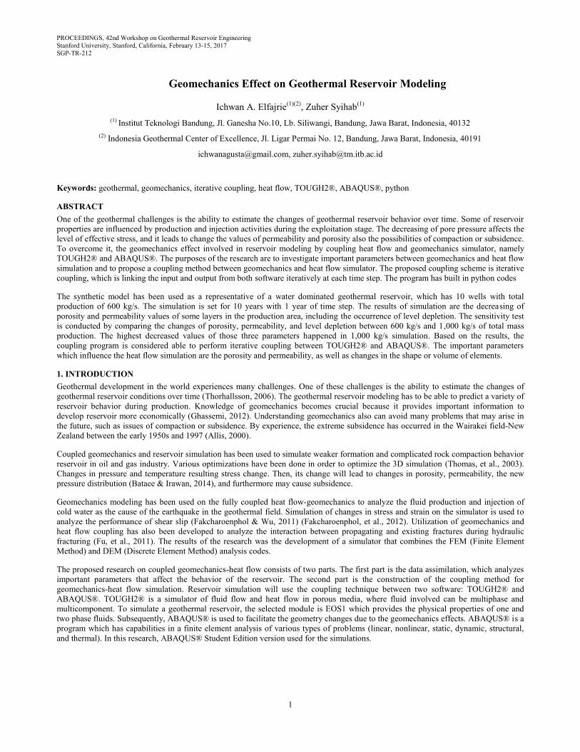
geomechanics simulators. Figure 1 shows the flowchart of the research methodology.

Elfajrie and Syihab

3

Figure 1: The research methodology

The similar reservoir model was constructed separately in TOUGH® and ABAQUS®. The connectivity between elements in

TOUGH2® is stated in MESH file, while the elements in ABAQUS® is connected by nodal number. The elements of reservoir model

in TOUGH2® must be well identified by both position and connectivity in ABAQUS®. This is necessary because for the same element

number in ABAQUS® has different position in TOUGH® model. Therefore, the coupling technique begins by synchronizing the

element of TOUGH2® and ABAQUS®.

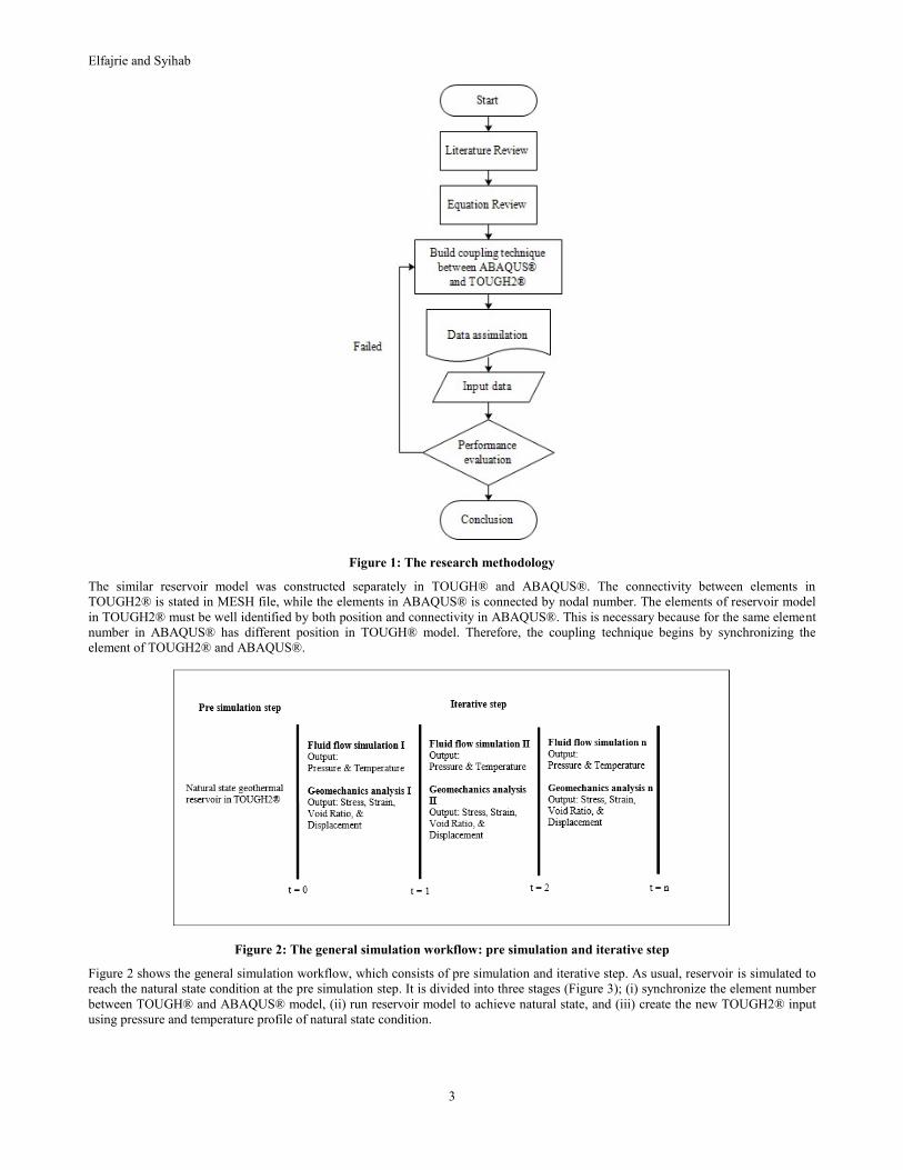
Figure 2: The general simulation workflow: pre simulation and iterative step

Figure 2 shows the general simulation workflow, which consists of pre simulation and iterative step. As usual, reservoir is simulated to

reach the natural state condition at the pre simulation step. It is divided into three stages (Figure 3); (i) synchronize the element number

between TOUGH® and ABAQUS® model, (ii) run reservoir model to achieve natural state, and (iii) create the new TOUGH2® input

using pressure and temperature profile of natural state condition.

Elfajrie and Syihab

4

Figure 3: The pre simulation workflow

The activity of read and write dataset of both software was driven automatically by python code. The iterative step consists of: (i) create

input TOUGH2®, (ii) run TOUGH2®, (iii) create input ABAQUS®, (iv) run ABAQUS® (Figure 4). The updated parameters of

TOUGH2® input are:

a. Porosity of rocks

b. Permeability in three axis (-x,-y, and –z) of rocks

c. Volume of element

d. Centroid position of each element

e. Connectivity (distance from centroid to contact surface and area plane)

f. Initial condition (temperature and pressure)

Figure 4: The iterative workflow

The new pressure and temperature distribution as the result of TOUGH2® simulation used to update the dataset of ABAQUS®. The

updated parameters of ABAQUS® input are:

a. Hydraulic conductivity

b. Bulk modulus

c. Temperature

The results of ABAQUS® simulation are the void ratio, nodal position, stress and strain distribution. The new permeability can be

updated by applying the new void ratio (porosity) into Equation (5). The change of geometry (represented by nodal position) used to

update the value of element centroid position (X, Y, Z) and volume (VOLX), distance between centroid to contact surface (D1, D2),

area plane and (AREAX). The porosity, permeability, and changes of geometry is representing the effect of geomechanics in heat flow

simulation.

4. MODELING

4.1 Model Structure

The synthetic model was created by adopting the Wairakei geothermal field, New Zealand. It is designed to be a representative of the

geothermal reservoir water dominated system. It covers 8.5 x 5 km area and consists of 11 horizontal layers with depth of 2.5 km.

Figure 5 shows the gridding at x-y cross section and layering system. The total thickness of reservoir was created to be 2 km, while the

heat source was located at the bottom of the layering system with 0.1 km of thickness. The third layer, cap rock, is 0.3 km thick and the

last layer of 0.1 km thick is represent surface. The reservoir is divided into 5 layers, each of 0.4 km thick, to facilitate the variety of

initial permeability. Totally, the model has 11 layers. Figure 5 shows the layering setting of the model.

The model coverage is quite extensive to resemble the actual geothermal reservoir. In order to model constant pressure and temperature,

the boundary condition has been set up by multiplying the volume factor to 1 x 1050 for boundary elements. The geothermal gradient

was set at 30oC/km on all elements.

Elfajrie and Syihab

5

5 km 2.5 km

8.5 km

(a) (b)

100 m 300 m

2,000 m

100 m

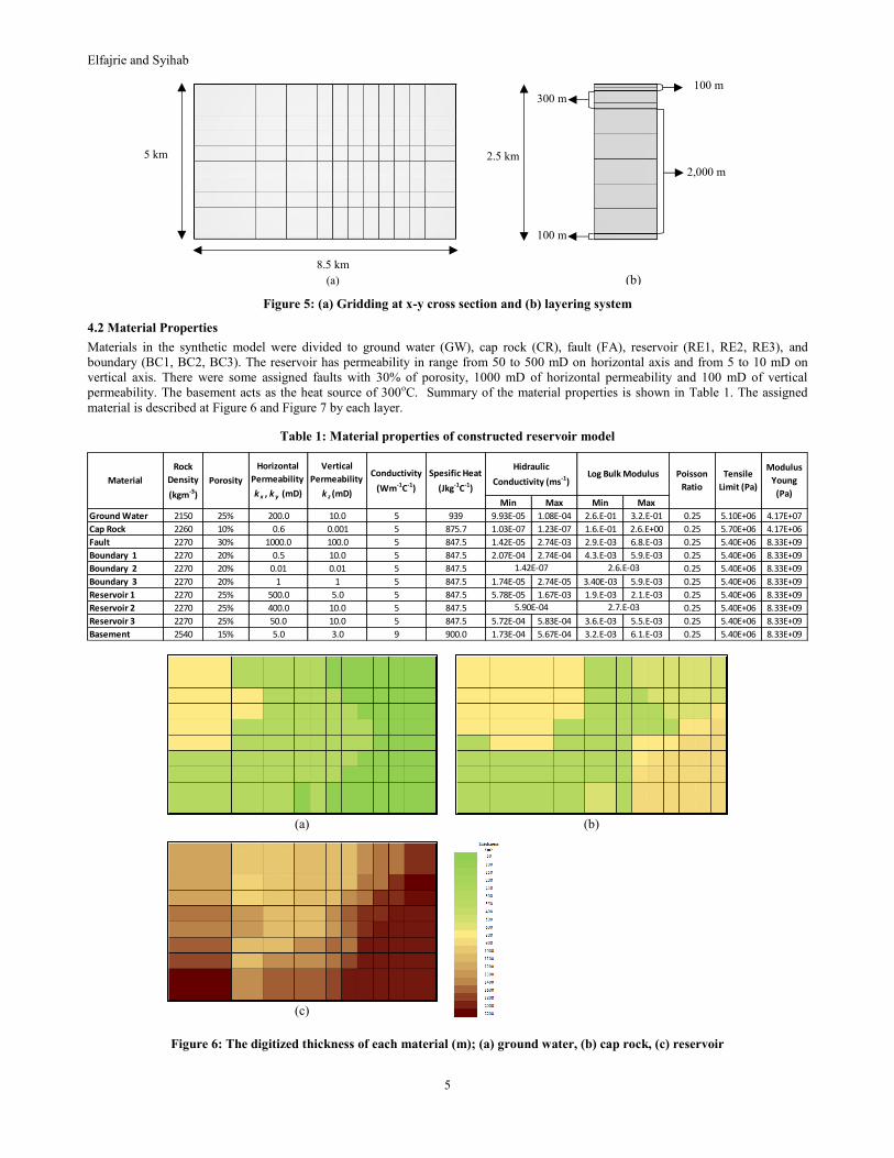
Figure 5: (a) Gridding at x-y cross section and (b) layering system

4.2 Material Properties

Materials in the synthetic model were divided to ground water (GW), cap rock (CR), fault (FA), reservoir (RE1, RE2, RE3), and

boundary (BC1, BC2, BC3). The reservoir has permeability in range from 50 to 500 mD on horizontal axis and from 5 to 10 mD on

vertical axis. There were some assigned faults with 30% of porosity, 1000 mD of horizontal permeability and 100 mD of vertical

permeability. The basement acts as the heat source of 300oC. Summary of the material properties is shown in Table 1. The assigned

material is described at Figure 6 and Figure 7 by each layer.

Table 1: Material properties of constructed reservoir model

(a)

(b)

(c)

Figure 6: The digitized thickness of each material (m); (a) ground water, (b) cap rock, (c) reservoir

Min Max Min Max

Ground Water 2150 25% 200.0 10.0 5 939 9.93E-05 1.08E-04 2.6.E-01 3.2.E-01 0.25 5.10E+06 4.17E+07

Cap Rock 2260 10% 0.6 0.001 5 875.7 1.03E-07 1.23E-07 1.6.E-01 2.6.E+00 0.25 5.70E+06 4.17E+06

Fault 2270 30% 1000.0 100.0 5 847.5 1.42E-05 2.74E-03 2.9.E-03 6.8.E-03 0.25 5.40E+06 8.33E+09

Boundary 1 2270 20% 0.5 10.0 5 847.5 2.07E-04 2.74E-04 4.3.E-03 5.9.E-03 0.25 5.40E+06 8.33E+09

Boundary 2 2270 20% 0.01 0.01 5 847.5 0.25 5.40E+06 8.33E+09

Boundary 3 2270 20% 1 1 5 847.5 1.74E-05 2.74E-05 3.40E-03 5.9.E-03 0.25 5.40E+06 8.33E+09

Reservoir 1 2270 25% 500.0 5.0 5 847.5 5.78E-05 1.67E-03 1.9.E-03 2.1.E-03 0.25 5.40E+06 8.33E+09

Reservoir 2 2270 25% 400.0 10.0 5 847.5 0.25 5.40E+06 8.33E+09

Reservoir 3 2270 25% 50.0 10.0 5 847.5 5.72E-04 5.83E-04 3.6.E-03 5.5.E-03 0.25 5.40E+06 8.33E+09

Basement 2540 15% 5.0 3.0 9 900.0 1.73E-04 5.67E-04 3.2.E-03 6.1.E-03 0.25 5.40E+06 8.33E+09

5.90E-04 2.7.E-03

1.42E-07 2.6.E-03

Material

Hidraulic

Conductivity (ms-1)Log Bulk Modulus

Modulus

Young

(Pa)

Tensile

Limit (Pa)

Poisson

Ratio

Spesific Heat

(Jkg-1C-1)

Conductivity

(Wm-1C-1)

Vertical

Permeability

k z (mD)

Horizontal

Permeability

k x , k y (mD)

Porosity

Rock

Density

(kgm-3)

Elfajrie and Syihab

6

(a) Layer 1 (L01)

(b) Layer 2 (L02)

(c) Layer 3 (L03)

(d) Layer 4 (L04)

(e) Layer 5 (L05)

(f) Layer 6 (L06)

(g) Layer 7 (L07)

(h) Layer 8 (L08)

(i) Layer 9 (L09)

(j) Layer 10 (L10)

(k) Layer 11 (L11)

Figure 7: The assigned material of each layer

4.3 Natural State

As a host of heat, the basement produces a constant value of 4.0 x 10-5 kgs-1m-2 and constant enthalpy at 1.15 x 106 Jkg-1. The boundary

condition set up for 1 x 1050 of volume factor. The pressure gradient follows hydrostatic equation, while temperature gradient applies

the geothermal gradient, 3oC per km, with 20oC of surface temperature. To achieve the natural state condition, the simulation run by

setting up the end time and maximum number of time steps to infinite. The convergence limit for each iteration is 1 x 10-4. The natural

state was achieved after 1,115,693,176.05 years. Figure 8 shows the temperature and pressure at natural state condition.

Figure 8: Temperature and pressure profile of natural state. The vectors define the heat flow per surface area (m2).

After the synthetic model has reached a natural state condition, ten production wells were drilled. The ten wells have total production of

600 kg/s or each well produces mass flow rate of 60 kg/s. The entire depth of the well reaches 2 km with similar productivity index (PI)

of 7 x 10-13 m3 and well head pressure (WHP) of 1 x 106 Pa. Figure 9 shows the position of the ten vertical wells on the model.

Figure 9: The location of production wells

Elfajrie and Syihab

7

To understand the geomechanics effect on coupled geomechanics-heat flow simulation, the specific element numbers chosen to be

analyzed. Analysis will be performed to each layer by averaging the values of permeability, porosity, displacement, pressure, and

temperature. The data of each layer are represented by the elements along the well. There are ten elements of each well, so that total

targeted elements are a hundred elements. Table 2 shows the list of all element number in each well.

Table 2: List of element number of each well

5. RESULT AND ANALYSIS

Simulation consists of two parts: the first part is a simulation without involving the effects of geomechanics and the second part is

coupled geomechanics-heat flow simulation. The simulation results between the two simulations are differences in the distribution of

pressure and temperature on some particular element. Other parameters measured were changes in porosity and permeability, as well as

changes in the nodal position of all elements of the production well during the ten years of production.

Sensitivity analysis of production rate was also conducted on coupled geomechanics-heat flow simulation. It varied into two types: high

(1,000 kg/s) and low flow rate (600 kg/s). Changes in porosity and permeability values of each flow rate categories was observed for a

qualitative understanding of the production rate.

5.1 Uncoupled Simulation

At this stage, the reservoir model is simulated by TOUGH2® only. Total fluid production was 600 kg/s, so that each well produced 60

kg/s. Figure 10 shows the pressure and temperature on average per layer in the area of production wells, where the reservoir is located

ranging from L03 to L07. Temperature profile is fairly constant in production layer annually.

Figure 10: Pressure and temperature profile on each layer in production area

5.2 Coupled Geomechanics-Heat Flow Simulation

The simulation results of coupled geomechanics-heat flow simulation showed the changes in the value of the porosity, permeability,

element volume, pressure, and temperature.

5.2.1. Temperature, Pressure, Porosity, and Permeability

Decrease in pore pressure will lead to changes in the value of void ratio (porosity). Figure 11 shows the change in the value of average

pressure and temperature of each layer. The simulation results of coupled geomechanics-heat flow show the difference in pressure and

temperature profile against uncoupled simulation results.

Well 1 Well 2 Well 3 Well 4 Well 5 Well 6 Well 7 Well 8 Well 9 Well 10

926 829 915 952 916 857 850 893 900 894

835 722 846 809 845 735 728 868 861 867

679 628 686 669 685 641 634 693 689 692

564 537 571 554 570 549 542 578 574 577

770 447 759 785 760 459 452 748 755 749

428 359 421 438 422 371 364 414 418 415

307 271 300 317 301 283 276 293 297 294

472 183 479 462 478 195 188 486 482 485

215 95 208 225 209 107 100 201 205 202

70 7 63 80 64 19 12 56 60 57

Element number of each well to depth

Elfajrie and Syihab

8

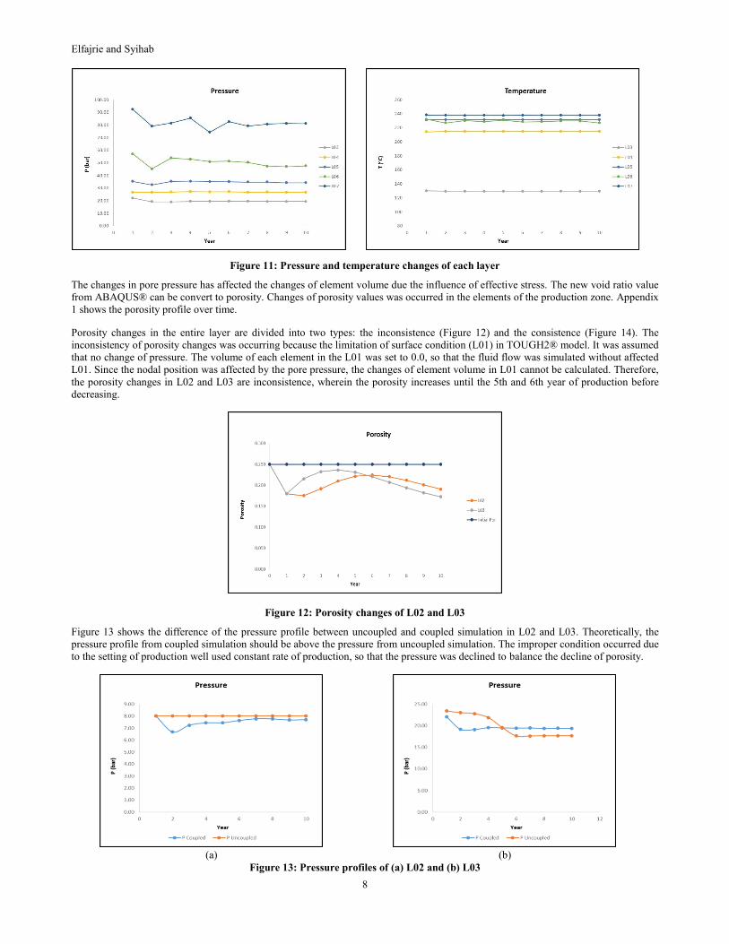
Figure 11: Pressure and temperature changes of each layer

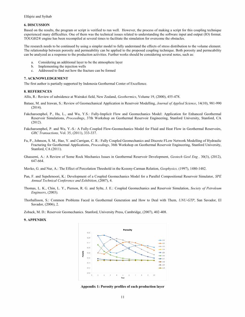
The changes in pore pressure has affected the changes of element volume due the influence of effective stress. The new void ratio value

from ABAQUS® can be convert to porosity. Changes of porosity values was occurred in the elements of the production zone. Appendix

1 shows the porosity profile over time.

Porosity changes in the entire layer are divided into two types: the inconsistence (Figure 12) and the consistence (Figure 14). The

inconsistency of porosity changes was occurring because the limitation of surface condition (L01) in TOUGH2® model. It was assumed

that no change of pressure. The volume of each element in the L01 was set to 0.0, so that the fluid flow was simulated without affected

L01. Since the nodal position was affected by the pore pressure, the changes of element volume in L01 cannot be calculated. Therefore,

the porosity changes in L02 and L03 are inconsistence, wherein the porosity increases until the 5th and 6th year of production before

decreasing.

Figure 12: Porosity changes of L02 and L03

Figure 13 shows the difference of the pressure profile between uncoupled and coupled simulation in L02 and L03. Theoretically, the

pressure profile from coupled simulation should be above the pressure from uncoupled simulation. The improper condition occurred due

to the setting of production well used constant rate of production, so that the pressure was declined to balance the decline of porosity.

(a)

(b)

Figure 13: Pressure profiles of (a) L02 and (b) L03

Elfajrie and Syihab

9

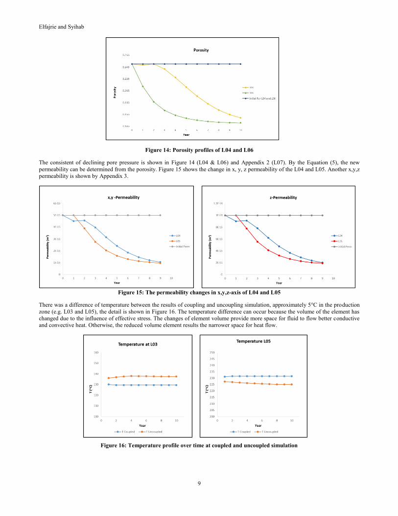
Figure 14: Porosity profiles of L04 and L06

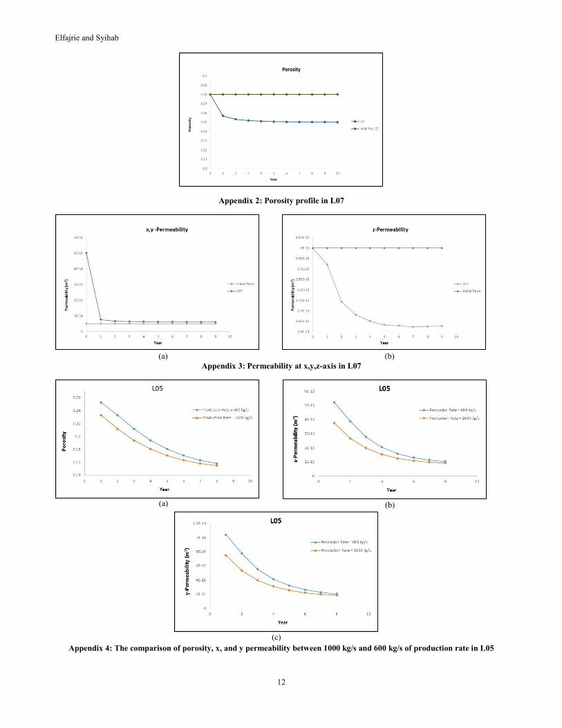
The consistent of declining pore pressure is shown in Figure 14 (L04 & L06) and Appendix 2 (L07). By the Equation (5), the new

permeability can be determined from the porosity. Figure 15 shows the change in x, y, z permeability of the L04 and L05. Another x,y,z

permeability is shown by Appendix 3.

Figure 15: The permeability changes in x,y,z-axis of L04 and L05

There was a difference of temperature between the results of coupling and uncoupling simulation, approximately 5°C in the production

zone (e.g. L03 and L05), the detail is shown in Figure 16. The temperature difference can occur because the volume of the element has

changed due to the influence of effective stress. The changes of element volume provide more space for fluid to flow better conductive

and convective heat. Otherwise, the reduced volume element results the narrower space for heat flow.

Figure 16: Temperature profile over time at coupled and uncoupled simulation

Elfajrie and Syihab

10

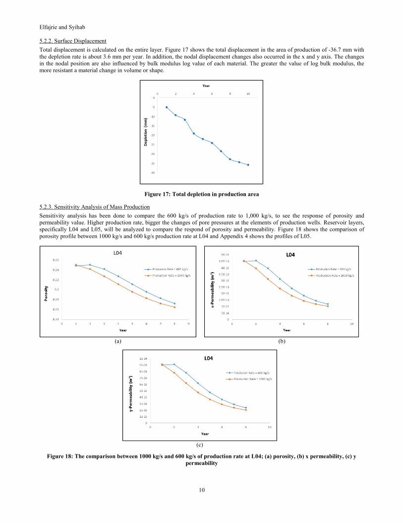
5.2.2. Surface Displacement Total displacement is calculated on the entire layer. Figure 17 shows the total displacement in the area of production of -36.7 mm with

the depletion rate is about 3.6 mm per year. In addition, the nodal displacement changes also occurred in the x and y axis. The changes

in the nodal position are also influenced by bulk modulus log value of each material. The greater the value of log bulk modulus, the

more resistant a material change in volume or shape.

Figure 17: Total depletion in production area

5.2.3. Sensitivity Analysis of Mass Production

Sensitivity analysis has been done to compare the 600 kg/s of production rate to 1,000 kg/s, to see the response of porosity and

permeability value. Higher production rate, bigger the changes of pore pressures at the elements of production wells. Reservoir layers,

specifically L04 and L05, will be analyzed to compare the respond of porosity and permeability. Figure 18 shows the comparison of

porosity profile between 1000 kg/s and 600 kg/s production rate at L04 and Appendix 4 shows the profiles of L05.

(a)

(b)

(c)

Figure 18: The comparison between 1000 kg/s and 600 kg/s of production rate at L04; (a) porosity, (b) x permeability, (c) y

permeability

Elfajrie and Syihab

11

6. DISCUSSION

Based on the results, the program or script is verified to run well. However, the process of making a script for this coupling technique

experienced many difficulties. One of them was the technical issues related to understanding the software input and output (IO) format.

TOUGH2® engine has been recompiled at several times to facilitate the simulation for overcome the obstacles.

The research needs to be continued by using a simpler model to fully understand the effects of stress distribution to the volume element.

The relationship between porosity and permeability can be applied to the proposed coupling technique. Both porosity and permeability

can be analyzed as a response to the production activities. Further works should be considering several notes, such as:

a. Considering an additional layer to be the atmosphere layer

b. Implementing the injection wells

c. Addressed to find out how the fracture can be formed

7. ACKNOWLEDGEMENT

The first author is partially supported by Indonesia Geothermal Center of Excellence.

8. REFERENCES

Allis, R.: Review of subsidence at Wairakei field, New Zealand, Geothermics, Volume 19, (2000), 455-478.

Bataee, M. and Irawan, S.: Review of Geomechanical Application in Reservoir Modelling, Journal of Applied Science, 14(10), 981-990

(2014).

Fakcharoenphol, P., Hu, L., and Wu, Y.S.: Fully-Implicit Flow and Geomechanics Model: Application for Enhanced Geothermal

Reservoir Simulations, Proceedings, 37th Workshop on Geothermal Reservoir Engineering, Stanford University, Stanford, CA

(2012).

Fakcharoenphol, P. and Wu, Y.-S.: A Fully-Coupled Flow-Geomechanics Model for Fluid and Heat Flow in Geothermal Reservoirs,

GRC Transactions, Vol. 35, (2011), 333-337.

Fu, P., Johnson, S. M., Hao, Y. and Carrigan, C. R.: Fully Coupled Geomechanics and Discrete FLow Network Modelling of Hydraulic

Fracturing for Geothermal Applications, Proceedings, 36th Workshop on Geothermal Reservoir Engineering, Stanford University,

Stanford, CA (2011).

Ghassemi, A.: A Review of Some Rock Mechanics Issues in Geothermal Reservoir Development, Geotech Geol Eng , 30(3), (2012),

647-664.

Mavko, G. and Nur, A.: The Effect of Percolation Threshold in the Kozeny-Carman Relation, Geophysics, (1997), 1480-1482.

Pan, F. and Sepehrnoori, K.: Development of a Coupled Geomechanics Model for a Parallel Compositional Reservoir Simulator, SPE

Annual Technical Conference and Exhibition, (2007), 4.

Thomas, L. K., Chin, L. Y., Pierson, R. G. and Sylte, J. E.: Coupled Geomechanics and Reservoir Simulation, Society of Petroleum

Engineers, (2003).

Thorhallsson, S.: Common Problems Faced in Geothermal Generation and How to Deal with Them, UNU-GTP, San Savador, El

Savador, (2006), 2.

Zoback, M. D.: Reservoir Geomechanics. Stanford, University Press, Cambridge, (2007), 402-408.

9. APPENDIX

Appendix 1: Porosity profiles of each production layer

Elfajrie and Syihab

12

Appendix 2: Porosity profile in L07

(a)

(b)

Appendix 3: Permeability at x,y,z-axis in L07

(a)

(b)

(c)

Appendix 4: The comparison of porosity, x, and y permeability between 1000 kg/s and 600 kg/s of production rate in L05