Geomagnetic Polarity Timescales and Reversal …rci.rutgers.edu/~dvk/dvk_REPRINTS/Lowrie+Kent2004.pdfGeomagnetic Polarity Timescales and Reversal Frequency Regimes William Lowrie ...

1. GEOMAGNETIC POLARITY TIMESCALES

The history of polarity reversals of Earth’s magnetic fieldis well known for the last 160 Myr from the record of oceanicmagnetic anomalies. Three distinct episodes are defined (Fig-ure 1). The youngest corresponds to the magnetic anomalies

Timescales of the Paleomagnetic FieldGeophysical Monograph Series 145Copyright 2004 by the American Geophysical Union10.1029/145GM09

117

Geomagnetic Polarity Timescales and ReversalFrequency Regimes

William Lowrie

Institute of Geophysics, ETH Hönggerberg, Zürich, Switzerland

Dennis V. Kent

Department of Geological Sciences, Rutgers University, Piscataway, New Jersey& Lamont-Doherty Earth Observatory, Palisades, New York

An analysis of geomagnetic reversal history is made for the most reliable polar-ity timescales covering the last 160 Myr. The timescale of Cande and Kent [1995](CK95) is the optimum representation of Cenozoic and Late Cretaceous polarityhistory, and the timescale of Channell et al. [1995] (CENT94) best represents the EarlyCretaceous and Late Jurassic. The CK95 timescale can be divided into two nearlylinear segments at Chron C12r. The lengths of chrons in the younger segment haveno systematic trend, and so this part of the polarity sequence is considered to be sta-tionary for statistical analysis. The mean chron length is 0.248 Myr and the gammaindex, k, for the distribution of chron lengths is 1.6 ± 0.4; inserting just 8 additionalshort subchrons that have been verified from magnetostratigraphic studies as polar-ity reversals reduces the mean chron length to 0.219 Myr and k to 1.3 ± 0.3. The oldersegment is stationary if the two long polarity chrons C33n and C33r adjacent to theCretaceous Normal Polarity Superchron are omitted; in this case the mean chronlength is 0.749 Myr and k is 1.2 ± 0.4. The chrons in the CENT94 timescale are sta-tionary with mean length 0.415 Myr and k is 1.3 ± 0.3. The gamma indices of thechron distributions are not significantly different from a Poisson distribution (k = 1),which implies that the reversal process is essentially free of long-term memory.However, if the mean chron duration is an indicator of stability of the reversalprocess, it appears that long lasting episodes of stable behavior may be followedby abrupt change to another stable regime with a markedly different reversal fre-quency. There is no significant change of the gamma index from one regime toanother although the mean polarity chron length changes by more than a factor ofthree. This would imply that the probability of a reversal may be constant within eachregime but varies inversely with mean interval length from regime to regime.

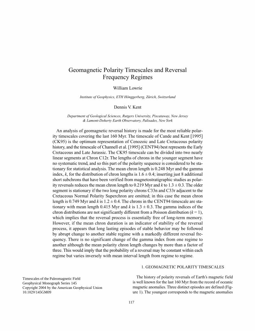
formed in the Cenozoic and Late Cretaceous, which are herereferred to as the C-sequence. This is separated in the oceanicrecord from the older M-sequence of anomalies, formed inLate Jurassic and early Cretaceous times, by the CretaceousQuiet Zone in which correlated magnetic anomalies are absent.The corresponding Cretaceous Normal Polarity Superchron(CNPS) represents a time interval in which Earth’s magneticfield evidently did not reverse polarity. Magnetic polaritystratigraphy studies in continental exposures of marine lime-stones have confirmed the main features of the C- andM-sequences as reflecting reversals of the geomagnetic fieldand correlated most stage boundaries from the Late Jurassicto the present to the corresponding marine magnetic polarityrecords [Alvarez et al., 1977; Channell and Erba, 1992; Chan-nell et al., 2000; Channell et al., 1979; Channell and Medi-zza, 1981; Lowrie and Alvarez, 1981; Lowrie and Alvarez,1984; Lowrie et al., 1982; Lowrie and Channell, 1984; Ogget al., 1984].

Several magnetic polarity timescales have been developed foreach of the two reversal sequences. In each case the magneticanomalies are first interpreted as a block model of oceaniccrustal magnetizations of alternating polarity. Multiple pro-files are combined to minimize local minor differences inspreading rate on any given profile. The spacings of blockboundaries in the resultant composite block model then definethe relative lengths of polarity intervals in the timescale. Mag-netic stratigraphy has played an important role in dating thepolarity sequences by correlating key biostratigraphic stageboundaries or other radiometrically dated datum-levels to theC- and M-sequence polarity record. The rest of the timescaleis dated by conversion of polarity boundary locations to numericages by interpolation between the tie-levels. In order to avoid

sudden changes in apparent spreading rate at tie-points a best-fit straight line or smooth curve may be fitted to the correla-tion points. The fundamental assumption here is that sea-floorspreading in selected corridors was constant or at least smoothlyvarying over long intervals of time, which is justified at leastto first order, but is nonetheless a potential source of error indetermining block widths and chron durations. The ‘absoluteages’ of the tie-levels are much less exactly known than therelative lengths of the polarity intervals. In addition to theerrors of absolute dating there are stratigraphic errors in relat-ing the radiometrically dated rocks to the biostratigraphicallylocated stage boundary or other datum-levels.

The polarity timescale for each reversal sequence hasevolved, accompanying improvements in the resolution ofmagnetic anomalies, definition of oceanic block models, mag-netostratigraphic correlation and the dating of calibrationpoints. The pioneering timescale of Heirtzler et al. [1968],hereafter referred to as HDHPL68, was derived from com-parison of marine magnetic profiles in different oceans, fromwhich a block model of crustal magnetization based on ahighly levered extrapolation of sea-floor spreading history inthe South Atlantic was chosen as best representative for anom-alies from the present to the Late Cretaceous (anomaly 32). TheLate Cretaceous anomaly sequence was refined and extendedto anomaly 33r by analyses of North Pacific and North Atlanticmarine profiles [Cande and Kristoffersen, 1977]. Magne-tostratigraphic correlation of the Cretaceous-Tertiary bound-ary to anomaly 29r [Lowrie and Alvarez, 1977] provided betterdating of the older end of the sequence. This resulted in amore accurate timescale [LaBrecque et al., 1977], hereafterreferred to as LKC77. These reversal sequences formed thebasis of several subsequent timescales [Mead, 1996].

A detailed re-evaluation of the C-sequence marine mag-netic anomalies and the corresponding block models led to thedevelopment of an improved timescale [Cande and Kent,1992a]. Age calibration was achieved by fitting a smooth(cubic spline) curve to nine calibration levels for South Atlanticspreading history. An updated version [Cande and Kent, 1995],hereafter referred to as CK95, incorporates improved agesfor the calibration levels. It is used as reference timescale forthe Late Cretaceous and Cenozoic (C-sequence) in the pres-ent paper.

Investigations of magnetic anomalies on the Hawaiian,Japanese and Phoenix lineations in the North Pacific and theKeathley lineations in the North Atlantic were integrated intoa polarity sequence and timescale covering marine magneticanomalies M0 to M25 [Larson and Hilde, 1975], which formedthe basis for subsequent polarity timescales. Oceanic crustolder than the sequence M0–M25 was at first thought to bedevoid of lineated magnetic anomalies and was called theJurassic Quiet Zone by analogy to its Cretaceous counterpart.

2 GEOMAGNETIC POLARITY TIMESCALES AND REVERSAL FREQUENCY REGIMES

Figure 1. Composite timescale incorporating the current optimumtimescales for the C-sequence and M-sequence magnetic anom-alies.

Magnetic lineations with low amplitude were described inthe youngest part of the Jurassic Quiet Zone and modeled bya block model of polarity characterized by decreasing mag-netization with increasing age [Cande et al., 1978]. TheM-sequence was extended thereby to M29.

The dating of M-sequence polarity reversals relied initiallyon estimated bottom ages in DSDP holes drilled on or near thelineations. Subsequent timescales have been formed by attach-ing better calibration ages to the sequence [Harland et al.,1990; Kent and Gradstein, 1985]. These usually consist of agroup of ages at each end, with linear interpolation and extrap-olation serving to date reversal boundaries between and beyondthe tie-points. Channell et al. [1995] compared block mod-els for the anomalies on the Hawaiian, Japanese, Phoenix andKeathley lineations and decided on a new Hawaiian blockmodel with optimum approximation to constant spreadingrate, covering magnetic polarity chrons CM0 to CM29. Thecalibration ages gave favorable comparison with stage bound-ary ages from magnetostratigraphic correlations. Thistimescale, hereafter CENT94, is chosen as reference for theM-sequence in this paper. The combined polarity timescalesrepresented by CK95 and CENT94 delineate a CretaceousNormal Polarity Superchron (CNPS) that began at 120.6 Maand lasted until 83.0 Ma (Figure 1).

Later airborne and marine deep-tow magnetometer surveyshave suggested that the young end of the Jurassic Quiet Zoneis characterized by low amplitude, short wavelength anom-alies that are lineated [Handschumacher et al., 1988; Sager etal., 1998]. If they are due to short polarity chrons, they extendthe polarity history associated with the M-sequence of anom-alies from CM29 to CM41, and suggest that the Jurassic QuietZone may have formed during an interval of rapidly varyingmagnetic polarity [Handschumacher et al., 1988; Sager etal., 1998], rather than constant polarity, as inferred for theCretaceous Quiet Zone. However, the pre-M29 anomaliesresemble “tiny wiggles” observed within the C-sequence andmany of the features may thus be due to paleointensity fluc-tuations [Cande and Kent, 1992b]. Magnetostratigraphic inves-tigations of Middle to Late Oxfordian limestone sections[Steiner et al., 1985] have described magnetozones with nor-mal and reverse polarity, but these have not yet been correlatedsatisfactorily to the marine polarity record. In the absence ofsuch confirmation, the possible chrons CM29–CM41 are notdiscussed further here.

2. REVERSAL FREQUENCY SINCE THE LATEJURASSIC

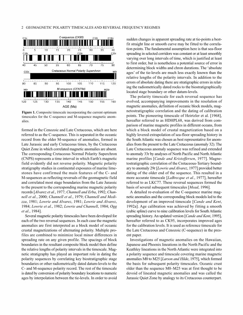
The variation of reversal behavior in the compositetimescale CK95+CENT94 is conveniently displayed by plot-ting the age of each reversal against the order of its occur-

rence (Figure 2). The CENT94 data closely define a straightline. The C-sequence can be divided into two nearly linearsegments that intersect near Chron C12r at about 31–33 Ma.We subdivide the polarity sequence at Chron C12r becausethis 2.1 Myr chron lasts about an order of magnitude longerthan the average subsequent chron. Two polarity intervals,C33n and C33r, immediately following the CNPS are severaltimes longer than any of the following chrons. They are thesecond and third longest chrons in the entire 160 Masequence and may have closer affinity to the CNPS than tothe rest of the polarity sequence. For the purposes of fur-ther analysis we define the segment younger than C12r asCK95(1) and the older segment (including C12r but withoutC33n and C33r) as CK95(2). This choice is somewhat arbi-trary but it allows us to subdivide the polarity sequence intothe longest possible linear segments without excluding anychrons other than C33n and C33r. Linear segments implythat the reversal process is stationary within the segmentand allow calculation of representative statistical parame-ters. Mean polarity interval lengths are 0.248 Myr forCK95(1), 0.749 Myr for CK95(2), and 0.415 Myr forCENT94. The CNPS, the 37.6 Myr Cretaceous interval ofconstant normal polarity, is evident as an abrupt disconti-nuity between the M- and C-sequences and may represent aprolonged disruption of the reversal process.

3. STATISTICAL ANALYSIS OF CHRON LENGTHS

3.1 Statistical Models of Polarity Chron Durations

The observed durations of polarity chrons (104–107 yr) aretypically much longer than the characteristic time constants ofmagnetohydrodynamic processes in Earth’s liquid core (102–104

yr). To account for the discrepancy, Cox [1968] proposed a sto-

LOWRIE AND KENT 3

Figure 2. Ages of magnetic reversals in the Cenozoic and Meso-zoicoceanic anomaly sequences, plotted against their age order.

chastic model in which the instantaneous probability of a rever-sal is constant. For a low probability of occurrence the lengths(x) of polarity chrons conform to an exponential (Poisson) dis-tribution with probability density function p(x) given by

in which µ is the mean chron length.This model was not, however, obviously supported by the

known geomagnetic polarity records, which were notablylacking in short polarity chrons. Instead, the observed distri-bution of chron durations usually agreed better with a gammadistribution [Naidu, 1970], which has the probability densityfunction

in which k is the gamma index of the distribution and ?(k) isthe gamma function of k, defined as

The exponential distribution corresponds to k = 1. A gammadistribution of chrons implies that the reversal process has amemory; the probability of a reversal is not constant withtime. Immediately after the occurrence of a reversal the prob-ability of a new one is at first very low and increases with

time. This would suggest that the reversal process has a recov-ery time during which the probability of a reversal is gradu-ally restored.

Estimation of the gamma index k usually employs themaximum likelihood method, first applied by Naidu [1970]to fixed windows and by Phillips [1977] to a moving window.In this method, the best estimate of k is the solution of theequation

where Ψ(k) = d{lnΓ(k)}/dk is the digamma function. Forsmall numbers of chrons, McFadden [1984] recommends thesubstitution of (N – 1) for N. The variance (σ2) of k is givenby the relationship [Phillips, 1977]

where Ψ′(k) = dΨ(k)/dk is the trigamma function. The ±2σconfidence limits of k may be estimated from this equation.

3.2 Results of Earlier Statistical Analyses

Non-stationarity of the reversal sequences complicates sta-tistical analyses of the chron durations. Naidu [1970] ana-lyzed the statistical properties of the HDHPL68 time-scale

2 1( )1'( )

kN k

k

σ = Ψ −

1ln ( ) ln lnN

k k xN

µ− Ψ = − ∑

10

( ) k xk x e dx∞ − −Γ = ∫

1( ) exp

( )

k kk x xp x kkµ µ

− = − Γ

1( ) exp xp xµ µ

= −

4 GEOMAGNETIC POLARITY TIMESCALES AND REVERSAL FREQUENCY REGIMES

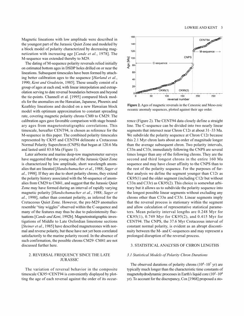
Figure 3. Polarity chron lengths (Myr) in three segments of the CK95 and CENT94 timescales, in which linear fits havenon-significant slopes.

within successive short windows of 8 Myr width. The assump-tion was made that the sequence was stationary in each shortwindow. The gamma index was estimated to be k = 2 forC-sequence polarity chrons younger than 48 Ma and k = 3.6for chrons older than 56 Ma.

A disadvantage of using fixed-width time windows is thatthe number of chrons in each window is different, which forsmall numbers might influence interpretation of the statis-tical properties. To obviate this problem Phillips [1977] ana-lyzed the HDHPL68 timescale with a moving windowcontaining a constant number of polarity intervals. Thismethod has the disadvantage that each window represents avariable length of time at different points in the sequence.Moreover, the window typically includes a rather small num-ber of chrons for robust statistical analysis. For chronsyounger than the discontinuity at 45 Ma, the gamma indexwas k = 1.55, but the analysis gave different values ofk = 2.28 and k = 1.19 for the distributions of normal and

reverse chrons, respectively. This was interpreted as indi-cating that the normal and reverse polarity states of Earth’smagnetic field have different stabilities.

Unfortunately, the pioneering HDHPL68 timescale wasincomplete and contained some erroneously interpreted polar-ity intervals, which gave rise to an artificial discontinuity inreversal rate at about 45 Ma. Thus the statistical analyses ofthis timescale have only historical significance.

Lowrie and Kent [1983] analyzed the improved LKC77timescale using a moving window of constant 8 Myr width.They found values of k = 1.52 for the stationary part of LKC77younger than 40 Ma; values of k = 1.90 and k = 1.28 werefound for the normal and reverse chrons, respectively, in thisinterval. McFadden and Merrill [1984] analyzed the LKC77timescale using 25-interval wide moving windows andobtained an optimum value of k = 1.25, with a 95% confi-dence range of 1.02 to 1.55. The difference in k between thenormal and reverse polarity states was attributed to over-sen-

LOWRIE AND KENT 5

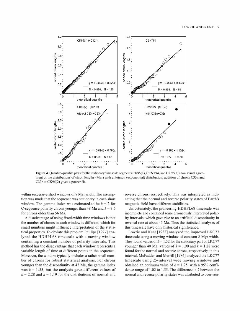
Figure 4. Quantile-quantile plots for the stationary timescale segments CK95(1), CENT94, and CK95(2) show visual agree-ment of the distributions of chron lengths (Myr) with a Poisson (exponential) distribution; addition of chrons C33n andC33r to CK95(2) gives a poorer fit.

sitivity of the analytical method rather than being a real fea-ture of the geomagnetic field.

A moving window analysis creates a false visual impressionthat the data set is larger than it really is; e.g., using a 25-pointmoving window, only every 25th analysis is independent. Ide-ally the entire timescale can be detrended by fitting a sui time-varying function for the mean value. Lutz and Watson [1988]and Gaffin [1989] modeled reversal rates with aperiodic func-

tions; Lowrie [1997] proposed using low-order polynomialsto represent the non-stationary mean chron length. Marzocchi[1997] detrended the CK95 timescale by fitting an exponen-tial to the reversal rate and obtained k = 1.4 ± 0.4 for the fulltimescale. He also found the part of CK95 younger than 30 Mato be stationary without detrending and obtained values of k= 1.6 ± 0.4 for this segment.

4. GAMMA INDEX ESTIMATION FOR C-SEQUENCEAND M-SEQUENCE CHRONS

A plot of the lengths of individual polarity chrons in thecomposite timescale against their occurrence [Gallet andCourtillot, 1995] is shown in Figure 3. Straight lines werefitted by least squares to the chron lengths and the Studentt-statistic was used to evaluate the confidence levels of theslopes. The best-fit line to CENT94, with 89 polarity intervals,has slope 0.0011 ± 0.0033 and is not significant. This con-clusion that there is no significant trend in CENT94 was alsoreached by Hulot and Gallet [2003] using a more sophisti-cated analysis of stationarity proposed by McFadden and Mer-rill [2000]. The slope of the linear segment CK95(1), with125 polarity intervals, is 0.0006 ± 0.0011 and is also not sig-nificant. These segments may be considered as stationary. Ifthe two very long polarity chrons C33n and C33r are includedin the analysis of segment CK95(2), the linear regression hasslope 0.0172 ± 0.0145 and is marginally significant. How-ever, if the two chrons are omitted, the best-fit line to theremaining 57 polarity intervals has slope 0.0050 ± 0.0112and is not significant.

The segments CK95(1), CK95(2) without C32r and C33r,and CENT94 are stationary. A quantile–quantile (Q–Q) test[Fisher et al., 1987] can be applied to the stationary segmentsto test visually how well the distributions of chron lengthsconform to a theoretical distribution, in this case the Poisson(exponential) distribution. To prepare this diagram, theobserved chrons are ranked in order of length and plottedagainst the theoretical quantile (Figure 4). The linear fits indi-cate good agreement with the Poisson distribution, except forCK95(2) when the long chrons C33n and C33r are included.This disagreement with the rest of the population is further jus-tification for omitting these two anomalously long chrons,which last 5.5 Myr and 3.9 Myr, respectively and togetherrepresent an appreciable fraction of the 83 Myr C-sequence.Their durations and location at the end of the CNPS suggestthat C33n and C33r might be more closely associated withthe kind of field behavior in the CNPS, which lasted 37.6Myr, rather than the more rapidly reversing later C-sequence.

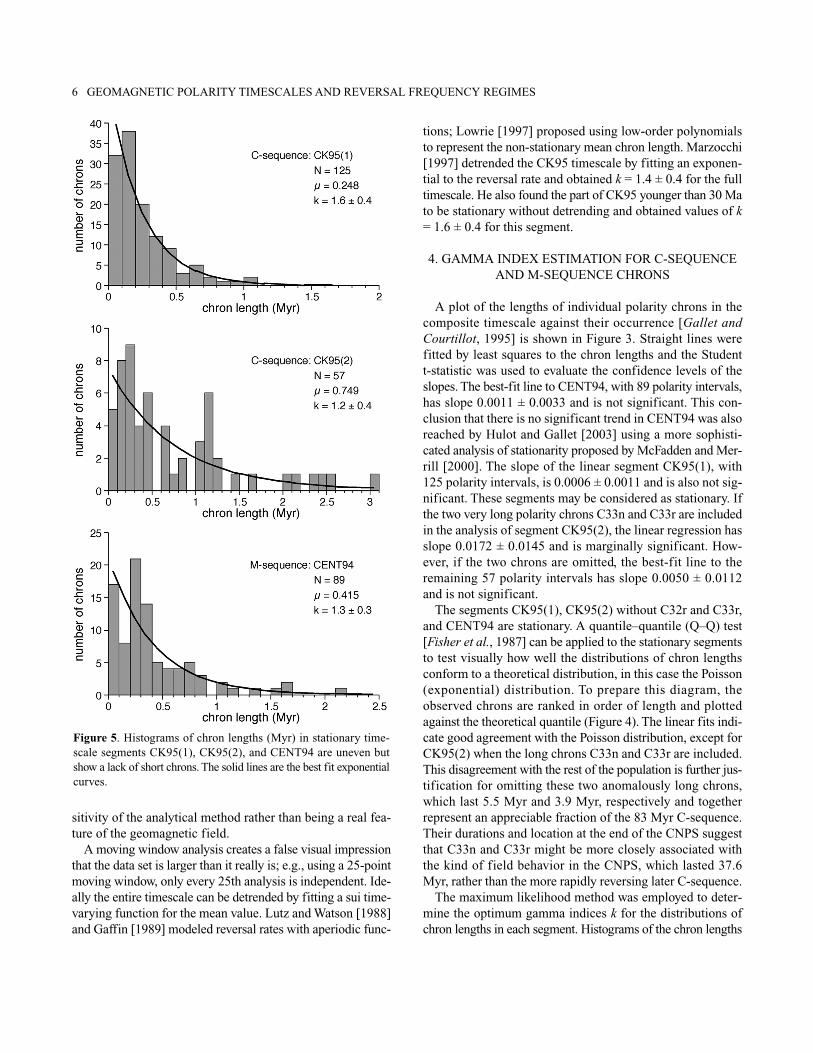
The maximum likelihood method was employed to deter-mine the optimum gamma indices k for the distributions ofchron lengths in each segment. Histograms of the chron lengths

6 GEOMAGNETIC POLARITY TIMESCALES AND REVERSAL FREQUENCY REGIMES

Figure 5. Histograms of chron lengths (Myr) in stationary time-scale segments CK95(1), CK95(2), and CENT94 are uneven butshow a lack of short chrons. The solid lines are the best fit exponentialcurves.

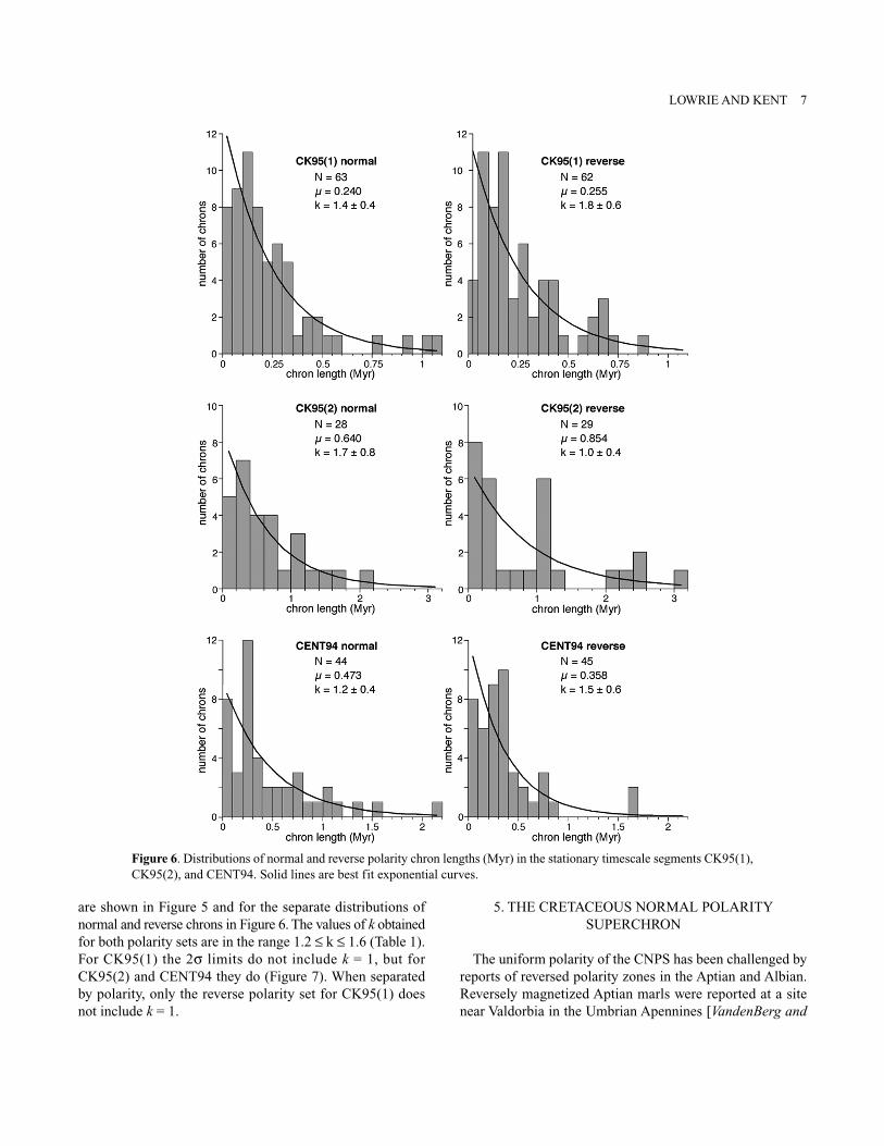
are shown in Figure 5 and for the separate distributions ofnormal and reverse chrons in Figure 6. The values of k obtainedfor both polarity sets are in the range 1.2 ≤ k ≤ 1.6 (Table 1).For CK95(1) the 2σ limits do not include k = 1, but forCK95(2) and CENT94 they do (Figure 7). When separatedby polarity, only the reverse polarity set for CK95(1) doesnot include k = 1.

5. THE CRETACEOUS NORMAL POLARITYSUPERCHRON

The uniform polarity of the CNPS has been challenged byreports of reversed polarity zones in the Aptian and Albian.Reversely magnetized Aptian marls were reported at a sitenear Valdorbia in the Umbrian Apennines [VandenBerg and

LOWRIE AND KENT 7

Figure 6. Distributions of normal and reverse polarity chron lengths (Myr) in the stationary timescale segments CK95(1),CK95(2), and CENT94. Solid lines are best fit exponential curves.

Wonders, 1976]. The magnetozone occurred in strongly hema-tized redbeds and was not found in other coeval Tethyan mag-netostratigraphic sections. However, Tarduno [1990] foundreversely magnetized samples of Aptian age in DSDP Site463. Although reversely magnetized beds were found in theAlbian Fucoid Marls in the Umbrian Contessa section, theirsignificance as polarity chrons was cast in doubt by rock mag-netic evidence that the magnetozone could be remagnetized[Tarduno et al., 1992]. Possible correlative short magneto-zones in cores recovered from the Deep Sea Drilling Programand Ocean Drilling Program may be due to accidentallyinverted core segments. There is presently no convincing evi-dence that refutes the interpretation of the CNPS as an unin-terrupted lengthy period of constant normal polarity, but thereare strong indications that it may be characterized by pale-ointensity fluctuations [Cronin et al., 2001].

6. EFFECTS OF CRYPTOCHRONS ON POLARITYCHRON DISTRIBUTIONS

Many short wavelength, low amplitude magnetic anom-alies (“tiny wiggles”) are interspersed in the marine magneticrecord. It is uncertain if these represent very short polaritychrons or geomagnetic intensity fluctuations. Cande andLaBrecque [1974] were able to model small scale magneticanomalies between Anomalies 5 and 5A equally satisfactorilyas either short chrons or intensity fluctuations. Cande andKent [1992b] made a detailed analysis of some of these anom-

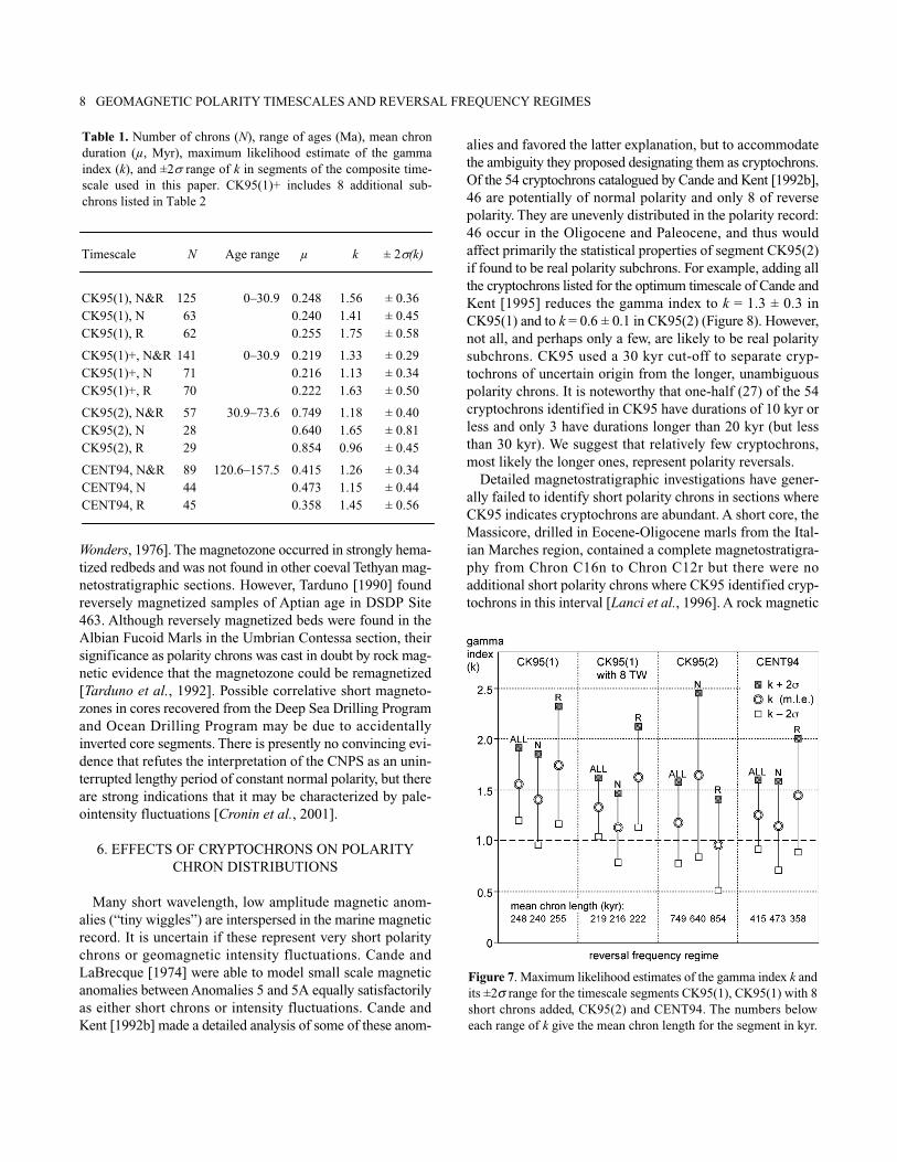
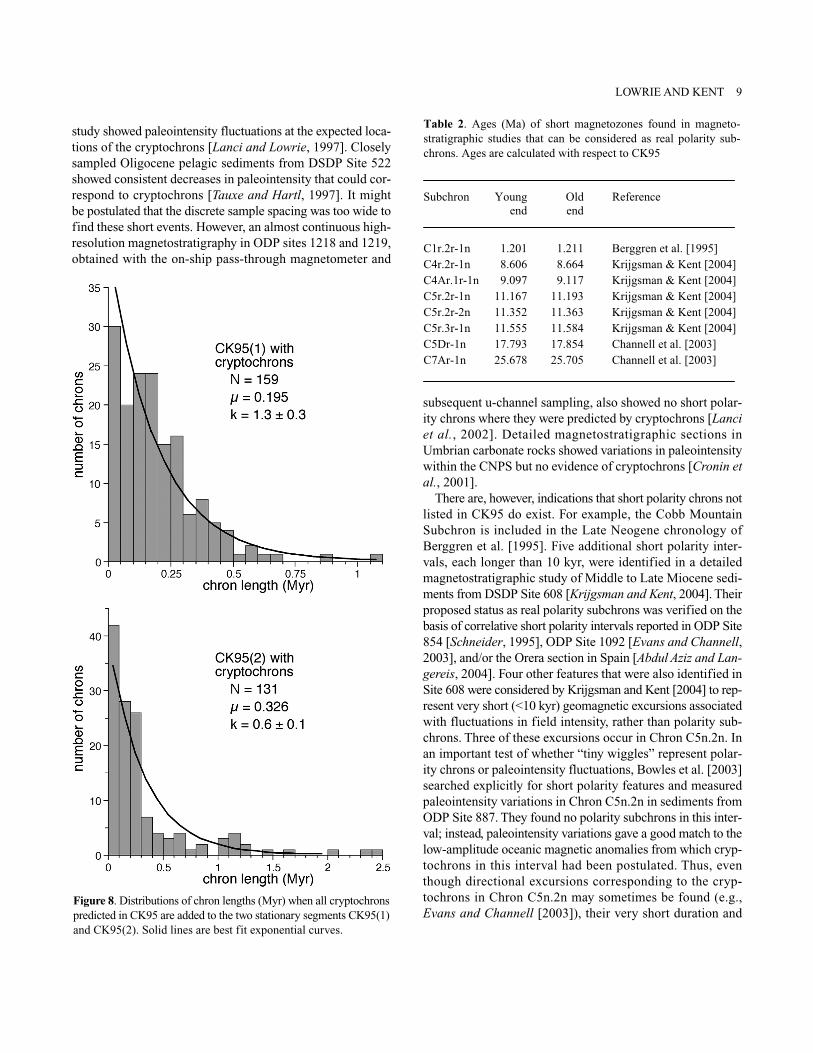
alies and favored the latter explanation, but to accommodatethe ambiguity they proposed designating them as cryptochrons.Of the 54 cryptochrons catalogued by Cande and Kent [1992b],46 are potentially of normal polarity and only 8 of reversepolarity. They are unevenly distributed in the polarity record:46 occur in the Oligocene and Paleocene, and thus wouldaffect primarily the statistical properties of segment CK95(2)if found to be real polarity subchrons. For example, adding allthe cryptochrons listed for the optimum timescale of Cande andKent [1995] reduces the gamma index to k = 1.3 ± 0.3 inCK95(1) and to k = 0.6 ± 0.1 in CK95(2) (Figure 8). However,not all, and perhaps only a few, are likely to be real polaritysubchrons. CK95 used a 30 kyr cut-off to separate cryp-tochrons of uncertain origin from the longer, unambiguouspolarity chrons. It is noteworthy that one-half (27) of the 54cryptochrons identified in CK95 have durations of 10 kyr orless and only 3 have durations longer than 20 kyr (but lessthan 30 kyr). We suggest that relatively few cryptochrons,most likely the longer ones, represent polarity reversals.

Detailed magnetostratigraphic investigations have gener-ally failed to identify short polarity chrons in sections whereCK95 indicates cryptochrons are abundant. A short core, theMassicore, drilled in Eocene-Oligocene marls from the Ital-ian Marches region, contained a complete magnetostratigra-phy from Chron C16n to Chron C12r but there were noadditional short polarity chrons where CK95 identified cryp-tochrons in this interval [Lanci et al., 1996]. A rock magnetic

8 GEOMAGNETIC POLARITY TIMESCALES AND REVERSAL FREQUENCY REGIMES

Figure 7. Maximum likelihood estimates of the gamma index k andits ±2σ range for the timescale segments CK95(1), CK95(1) with 8short chrons added, CK95(2) and CENT94. The numbers beloweach range of k give the mean chron length for the segment in kyr.

study showed paleointensity fluctuations at the expected loca-tions of the cryptochrons [Lanci and Lowrie, 1997]. Closelysampled Oligocene pelagic sediments from DSDP Site 522showed consistent decreases in paleointensity that could cor-respond to cryptochrons [Tauxe and Hartl, 1997]. It mightbe postulated that the discrete sample spacing was too wide tofind these short events. However, an almost continuous high-resolution magnetostratigraphy in ODP sites 1218 and 1219,obtained with the on-ship pass-through magnetometer and

subsequent u-channel sampling, also showed no short polar-ity chrons where they were predicted by cryptochrons [Lanciet al., 2002]. Detailed magnetostratigraphic sections inUmbrian carbonate rocks showed variations in paleointensitywithin the CNPS but no evidence of cryptochrons [Cronin etal., 2001].

There are, however, indications that short polarity chrons notlisted in CK95 do exist. For example, the Cobb MountainSubchron is included in the Late Neogene chronology ofBerggren et al. [1995]. Five additional short polarity inter-vals, each longer than 10 kyr, were identified in a detailedmagnetostratigraphic study of Middle to Late Miocene sedi-ments from DSDP Site 608 [Krijgsman and Kent, 2004]. Theirproposed status as real polarity subchrons was verified on thebasis of correlative short polarity intervals reported in ODP Site854 [Schneider, 1995], ODP Site 1092 [Evans and Channell,2003], and/or the Orera section in Spain [Abdul Aziz and Lan-gereis, 2004]. Four other features that were also identified inSite 608 were considered by Krijgsman and Kent [2004] to rep-resent very short (<10 kyr) geomagnetic excursions associatedwith fluctuations in field intensity, rather than polarity sub-chrons. Three of these excursions occur in Chron C5n.2n. Inan important test of whether “tiny wiggles” represent polar-ity chrons or paleointensity fluctuations, Bowles et al. [2003]searched explicitly for short polarity features and measuredpaleointensity variations in Chron C5n.2n in sediments fromODP Site 887. They found no polarity subchrons in this inter-val; instead, paleointensity variations gave a good match to thelow-amplitude oceanic magnetic anomalies from which cryp-tochrons in this interval had been postulated. Thus, eventhough directional excursions corresponding to the cryp-tochrons in Chron C5n.2n may sometimes be found (e.g.,Evans and Channell [2003]), their very short duration and

LOWRIE AND KENT 9

Figure 8. Distributions of chron lengths (Myr) when all cryptochronspredicted in CK95 are added to the two stationary segments CK95(1)and CK95(2). Solid lines are best fit exponential curves.

ephemeral character suggest that they do not correspond toglobal polarity subchrons.

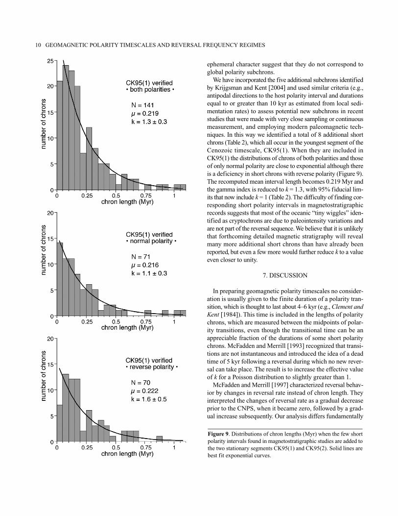
We have incorporated the five additional subchrons identifiedby Krijgsman and Kent [2004] and used similar criteria (e.g.,antipodal directions to the host polarity interval and durationsequal to or greater than 10 kyr as estimated from local sedi-mentation rates) to assess potential new subchrons in recentstudies that were made with very close sampling or continuousmeasurement, and employing modern paleomagnetic tech-niques. In this way we identified a total of 8 additional shortchrons (Table 2), which all occur in the youngest segment of theCenozoic timescale, CK95(1). When they are included inCK95(1) the distributions of chrons of both polarities and thoseof only normal polarity are close to exponential although thereis a deficiency in short chrons with reverse polarity (Figure 9).The recomputed mean interval length becomes 0.219 Myr andthe gamma index is reduced to k = 1.3, with 95% fiducial lim-its that now include k = 1 (Table 2). The difficulty of finding cor-responding short polarity intervals in magnetostratigraphicrecords suggests that most of the oceanic “tiny wiggles” iden-tified as cryptochrons are due to paleointensity variations andare not part of the reversal sequence. We believe that it is unlikelythat forthcoming detailed magnetic stratigraphy will revealmany more additional short chrons than have already beenreported, but even a few more would further reduce k to a valueeven closer to unity.

7. DISCUSSION

In preparing geomagnetic polarity timescales no consider-ation is usually given to the finite duration of a polarity tran-sition, which is thought to last about 4–6 kyr (e.g., Clement andKent [1984]). This time is included in the lengths of polaritychrons, which are measured between the midpoints of polar-ity transitions, even though the transitional time can be anappreciable fraction of the durations of some short polaritychrons. McFadden and Merrill [1993] recognized that transi-tions are not instantaneous and introduced the idea of a deadtime of 5 kyr following a reversal during which no new rever-sal can take place. The result is to increase the effective valueof k for a Poisson distribution to slightly greater than 1.

McFadden and Merrill [1997] characterized reversal behav-ior by changes in reversal rate instead of chron length. Theyinterpreted the changes of reversal rate as a gradual decreaseprior to the CNPS, when it became zero, followed by a grad-ual increase subsequently. Our analysis differs fundamentally

10 GEOMAGNETIC POLARITY TIMESCALES AND REVERSAL FREQUENCY REGIMES

Figure 9. Distributions of chron lengths (Myr) when the few shortpolarity intervals found in magnetostratigraphic studies are added tothe two stationary segments CK95(1) and CK95(2). Solid lines arebest fit exponential curves.

from theirs because we see evidence for stationary reversalbehavior prior to and after the CNPS. In this respect, our pointof view is more similar to that of Gallet and Hulot [1997],who regarded the CNPS as representing either an abrupt per-turbation of the reversal process or a separate (non)reversalregime rather than being part of a continuous, long-term evo-lution of reversal rate. The stationarity prior to the CNPS is inagreement with the findings of Hulot and Gallet [2003] thatthere is little evidence of precursory field behavior that her-alded this superchron, contrary to the earlier suggestion ofMcFadden and Merrill [2000].

Although our analysis reaches similar conclusions, it differsin several ways from that of Gallet and Hulot [1997]. They sub-divide the polarity sequence into three segments on the basis ofage, at points that differ from ours and for different criteria.Their segment A, covering 130–160 Ma, omits the youngestM-chrons; it is stationary, which we find to be the case for allof CENT94 from 120–160 Ma, including the youngestM-chrons. Segment B of Gallet and Hulot [1997], covering25–130 Ma, includes the CNPS and is not stationary. Merrill andMcFadden [1994] found it inappropriate to consider the CNPSas part of the reversal sequence in statistical analyses; we alsoomit it from our analysis. In addition, we omit chrons C33nand C33r, which in our view have a similar status to the CNPS.These omissions result in a stationary segment CK95(2). Seg-ment A of Gallet and Hulot [1997], covering 0–25 Ma, is sta-tionary. Our CK95(1) embraces 0–31 Ma and is stationary, aconclusion also reached by Marzocchi [1997].

We note here that the pre-CM29 cryptochrons in the marineanomaly record have the same character as the “tiny wiggles”in the Cenozoic record and, moreover, have not been correlatedsatisfactorily in magnetostratigraphic studies. We haveexcluded the pre-CM29 features because the reversal sequencethey might represent has not been verified and the anomaliesmay well be due to paleointensity variations. If they should befound to represent reversals, they should then be regarded aspart of a (higher frequency) reversal regime distinct fromCENT94, as CK95(1) is distinct from CK95(2).

The increasing reversal rate following the CNPS in theanalyses of McFadden and Merrill [1997] and McFadden andMerrill [2000] arises because they consider the C-sequence inits entirety to be non-stationary, whereas we regard it as com-posed of two reversal regimes, each of which is stationary.Chrons C33r and C33n immediately following the CNPS, ifincluded in CK95(2), would make this segment barely non-sta-tionary. However, they are exceptionally long and might wellbe classified with the CNPS; together, these chrons can evenbe considered as a different reversal regime with an excep-tionally long mean interval length of 15.7 Myr.

In some previous analyses of reversal statistics, values ofk substantially greater than 1 were regarded as due to either

an incomplete record or some process that inhibits rever-sals. McFadden and Merrill [1984] regarded a value of kgreater than 1 as an indicator for the fraction of missed shortpolarity chrons that were not resolved in the polaritytimescales because of concatenation with other chrons. Theypredicted that about 46% of the polarity intervals in the C-sequence contained one or more unresolved short chrons.This prediction has not stood the test of observation. Themost detailed analysis of the Late Cretaceous and Cenozoicreversal record, CK95, identified 54 locations where shortpolarity chrons might occur. Yet few of these cryptochronshave been confirmed as polarity intervals, as summarizedabove. Moreover, the addition of only 8 verified subchronsin CK95(1) has reduced k to be statistically indistinguishablefrom 1 (Poissonian, taking into account finite transitiontime), whereas CENT94 and CK95(2) already have gammaindices statistically indistinguishable from 1. Should moresubchrons be confirmed, they would further reduce k to avalue even closer to unity in each regime. Interestingly, thereis remarkably little difference in the k-values for CK95(1) ifonly 8 selected subchrons from magnetostratigraphy or all 17possible cryptochrons from CK95 are added. This is an indi-cation that the statistical properties are becoming very robust.The general absence of short polarity intervals in the CNPSmay indicate that the occurrence of cryptochrons is a func-tion of reversal rate, i.e., more might be expected to occurwhen the geodynamo is already reversing frequently, as insegment CK95(1).

In another scenario, the reversal itself is treated as a specialevent, following which there is an ‘inhibition’ period of 40–50kyr in which the probability of another reversal is reduced[McFadden and Merrill, 1993]. Such an inhibition period,whose physical origin is unclear, was introduced in order toexplain elevated values of k when the mean interval lengthwas short. However, given our observation that there is nosignificant change in gamma index k with mean intervallength, and that k is close to unity in each reversal regime,the concept of an inhibition period is unnecessary.

Our analysis leads to the following conclusions.(1) The record of reversal history over the past 160 Myr is

composed of distinct segments in which the reversalprocess was stationary and characterized by a gammaindex not distinctly different from unity, i.e. a Poissonprocess.

(2) Each segment may be looked on as a different regime ofreversal behavior, either intrinsic to the dynamo process ortriggered externally, e.g., see Gallet and Hulot [1997].Further progress in understanding the significance of thereversal regimes will require integration of other relevanttypes of data, such as paleosecular variation [McFadden etal., 1991].

LOWRIE AND KENT 11

(3) From one regime to another there is no significant changein gamma index k, but the average reversal rates shiftabruptly and markedly, for example by a factor 3 in theCenozoic.

(4) The Poisson model, with k indistinguishable from 1,appears to be a fundamental feature of geomagnetic fieldreversals. It is not only characteristic of the last 160 Myras documented here for CK95(1), CK95(2), and CENT94.It is also observed for a 30 Myr interval in the Late Triassic,for which an astronomically calibrated geomagnetic polar-ity timescale has been developed [Kent and Olsen, 1999].

Acknowledgements. This is contribution 6552 of Lamont DohertyEarth Observatory and contribution 1323 of the Institute of Geo-physics, ETH Zürich. DVK is grateful to the ETH Zürich for partialsupport during a sabbatical visit. We thank Ron Merrill and YvesGallet for helpful reviews.

REFERENCES

Abdul Aziz, H., and C. G. Langereis, Geomagnetic polarity time-scales and reversal frequency regimes, in Chapman Conference onTimescales of the Geomagnetic Field, edited by J. E. T. Channell,D. V. Kent, W. Lowrie, and J. Meert, American Geophysical Union,Gainesville, Florida, 2004.

Alvarez, W., M. A. Arthur, A. G. Fischer, W. Lowrie, G. Napoleone,I. Premoli Silva, and W. M. Roggenthen, Upper Cretaceous-Pale-ocene magnetic stratigraphy at Gubbio, Italy. V. Type section forthe Late Cretaceous-Paleocene geomagnetic reversal time scale,Geol. Soc. Amer. Bull., 88, 383–389, 1977.

Berggren, W. A., F. J. Hilgen, C. G. Langereis, D. V. Kent, J. D.Obradovich, I. Raffi, M.E. Raymo, and N. J. Shackleton, LateNeogene chronology: New perspectives in high-resolution stratig-raphy, Geol. Soc. Amer. Bull., 107, 1272–1287, 1995.

Bowles, J., L. Tauxe, J. Gee, D. McMillan, and S. Cande, Source oftiny wiggles in chron C5A: A comparison of sedimentary rela-tive intensity and marine magnetic anomalies, Geochem., Geo-phys., Geosys., 4, doi:10.1029/2002GC000489, 2003.

Cande, S., R. L. Larson, and J. L. LaBrecque, Magnetic lineations inthe Pacific Jurassic quiet zone, Earth Planet. Sci. Lett., 41,434–440, 1978.

Cande, S. C., and D. V. Kent, A new geomagnetic polarity time scalefor the Late Cretaceous and Cenozoic, J. Geophys. Res., 97,13,917–13,951, 1992a.

Cande, S. C., and D. V. Kent, Ultra-high resolution marine magneticanomaly-profiles: a record of continuous paleointensity varia-tions?, J. Geophys. Res., 97, 15,075–15,083, 1992b.

Cande, S. C., and D. V. Kent, Revised calibration of the geomag-netic polarity timescale for the Late Cretaceous and Cenozoic, J.Geophys. Res., 100, 6093–6095, 1995.

Cande, S. C., and Y. Kristoffersen, Late Cretaceous magnetic anom-alies in the North Atlantic, Earth Planet. Sci. Lett., 35, 215–224,1977.

Cande, S. C., and J. L. LaBrecque, Behaviour of the earth’s palaeo-magnetic field from small scale marine magnetic anomalies,Nature, 247, 26–28, 1974.

Channell, J. E. T., and E. Erba, Early Cretaceous polarity chronsCM0 to CM11 recorded in northern Italian land sections nearBrescia, Earth Planet. Sci. Lett., 108, 161–179, 1992.

Channell, J. E. T., E. Erba, G. Muttoni, and F. Tremolada, Early Cre-taceous magnetic stratigraphy in the APTICORE drill core andadjacent outcrop at Cismon (Southern Alps, Italy), and correlationto the proposed Barremian-Aptian boundary stratotype, Geol.Soc. Amer. Bull., 112, 1430–1443, 2000.

Channell, J. E. T., E. Erba, M. Nakanishi, and K. Tamaki, Late Juras-sic-Early Cretaceous time scales and oceanic magnetic anomalyblock models, in Geochronology, Timescales, and StratigraphicCorrelation, Special Publication, SEPM, edited by W.A. Berggren,D. V. Kent, M. Aubry, and J. Hardenbol, pp. 51–64, 1995.

Channell, J. E. T., W. Lowrie, and F. Medizza, Middle and Early Cre-taceous magnetic stratigraphy from the Cismon section, northernItaly, Earth Planet. Sci. Lett., 42, 153–166, 1979.

Channell, J. E. T., and F. Medizza, Upper Cretaceous and Paleogenemagnetic stratigraphy and biostratigraphy from the Venetian(Southern) Alps, Earth Planet. Sci. Lett., 55, 419–432, 1981.

Clement, B. M., and D. V. Kent, Latitudinal dependency of geomag-netic polarity transition durations, Nature, 310, 488–491, 1984.

Cox, A., Lengths of geomagnetic polarity intervals, J. Geophys. Res.,73, 3247–3260, 1968.

Cronin, M., L. Tauxe, C. Constable, P. Selkin, and T. Pick, Noise inthe quiet zone, Earth Planet. Sci. Lett., 190, 13–30, 2001.

Evans, H. F., and J. E. T. Channell, Upper Miocene magnetic stratig-raphy at ODP site 1092 (sub-Antarctic South Atlantic): recogni-tion of ‘cryptochrons’ in C5n.2n, Geophysical J. Intl., 153,483–496, 2003.

Fisher, N. I., T. Lewis, and B. J. Embleton, Statistical Analysis ofSpherical Data, Cambridge University Press, 1987.

Gaffin, S., Analysis of scaling in the geomagnetic polarity reversalrecord, Phys. Earth Planet. Inter., 57, 284–290, 1989.

Gallet, Y., and V. Courtillot, Geomagnetic reversal behaviour since100 Ma, Phys. Earth Planet. Inter., 92, 235–244, 1995.

Gallet, Y., and G. Hulot, Stationary and nonstationary behaviourwithin the geomagnetic polarity time scale, Geophys. Res. Lett.,24, 1875–1878, 1997.

Handschumacher, D. W., W. W. Sager, T. W. C. Hilde, andD. R. Bracey, Pre-Cretaceous evolution of the Pacific plate andextension of the geomagnetic polarity reversal time scale withimplications for the origin of the Jurassic “Quiet Zone”, Tectono-physics, 155, 365–380, 1988.

Harland, W. B., R. L. Armstrong, A. V. Cox, L. E. Craig, A. G. Smith,and D.G. Smith, A Geologic Time Scale 1989, 263 pp., CambridgeUniversity Press, Cambridge, 1990.

Heirtzler, J. R., G. O. Dickson, E. M. Herron, W. C. Pitman, III, andX. Le Pichon, Marine magnetic anomalies, geomagnetic fieldreversals and motions of the ocean floor and continents, J. Geo-phys. Res., 73, 2119–2136, 1968.

Hulot, G., and Y. Gallet, Do superchrons occur without any palaeo-magnetic warning?, Earth Planet. Sci. Lett., 210, 191–201, 2003.

12 GEOMAGNETIC POLARITY TIMESCALES AND REVERSAL FREQUENCY REGIMES

Kent, D. C., and P. E. Olsen, Astronomically tuned geomagneticpolarity timescale for the Late Triassic, J. Geophys. Res., 104,12,831–12,841, 1999.

Kent, D. V., and F. M. Gradstein, A Cretaceous and Jurassicgeochronology, Geol. Soc. Am. Bull., 96, 1419–1427, 1985.

Krijgsman, W., and D. V. Kent, Non-uniform occurrence of short-termpolarity fluctuations in the geomagnetic field? New results fromMiddle to Late Miocene sediments of the North Atlantic (DSDPSite 608), AGU Monograph, 2004.

LaBrecque, J. L., D. V. Kent, and S. C. Cande, Revised magneticpolarity time scale for Late Cretaceous and Cenozoic time, Geol-ogy, 5, 330–335, 1977.

Lanci, L., J. M. Pares, and J. E. T. Channell, Miocene-Oligocenemagnetostratigraphy from Equatorial Pacific sediments (ODPSite 1218, Leg 199), Eos Trans. AGU, 83 (47), Fall Meeting Suppl.,Abstract PP21D-09, 2002.

Lanci, L., and W. Lowrie, Magnetostratigraphic evidence that “tinywiggles” in the marine magnetic anomaly record represent geo-magnetic paleointensity variations, Earth Planet. Sci. Lett., 148,581–592, 1997.

Lanci, L., W. Lowrie, and A. Montanari, Magnetostratigraphy of theEocene-Oligocene boundary in a short continental drill-core, EarthPlanet. Sci. Lett., 143, 37–48, 1996.

Larson, R. L., and T. W. C. Hilde, A revised time scale of magneticreversals for the Early Cretaceous and Late Jurassic, J. Geophys.Res, 80, 2586–2594, 1975.

Lowrie, W., Polynomial representation of geomagnetic polarity rever-sal sequences, EoS Trans. AGU, 78, F193, 1997.

Lowrie, W., and W. Alvarez, Upper Cretaceous-Paleocene magneticstratigraphy at Gubbio, Italy. III. Upper Cretaceous magneticstratigraphy, Geol. Soc. Amer. Bull., 88, 374–377, 1977.

Lowrie, W., and W. Alvarez, One hundred million years of geomag-netic polarity history, Geology, 9, 392–397, 1981.

Lowrie, W., and W. Alvarez, Lower Cretaceous magnetic stratigraphyin Umbrian pelagic limestone sections, Earth Planet. Sci. Lett., 71,315–328, 1984.

Lowrie, W., W. Alvarez, G. Napoleone, K. Perch-Nielsen, I. PremoliSilva, and M. Toumarkine, Paleogene magnetic stratigraphy inUmbrian pelagic carbonate rocks: the Contessa sections, Gubbio,Geol. Soc. Amer. Bull., 93, 414–432, 1982.

Lowrie, W., and J. E. T. Channell, Magnetostratigraphy of the Juras-sic-Cretaceous boundary in the Maiolica limestone (Umbria, Italy),Geology, 12, 44–47, 1984.

Lowrie, W., and D. V. Kent, Geomagnetic reversal frequency since theLate Cretaceous, Earth Planet. Sci. Lett., 62, 305–313, 1983.

Lutz, T. M., and G. S. Watson, Effects of long-term variation on thefrequency spectrum of the geomagnetic reversal record, Nature,334, 240–242, 1988.

Marzocchi, W., Missing reversals in the geomagnetic polaritytimescale: their influence on the analysis and in constraining theprocess that generates geomagnetic reversals, J. Geophys. Res.,102, 5157–5171, 1997.

McFadden, P. L., Statistical tools for the analysis of geomagneticreversal sequences, J. Geophys. Res., 89, 3363–3372, 1984.

McFadden, P. L., and R. T. Merrill, Lower mantle convection andgeomagnetism, J. Geophys. Res., 89, 3354–3362, 1984.

McFadden, P. L., and R. T. Merrill, Inhibition and geomagnetic fieldreversals, J. Geophys. Res., 98, 6189–6199, 1993.

McFadden, P. L., and R. T. Merrill, Asymmetry in the reversal ratebefore and after the Cretaceous Normal Polarity Superchron, EarthPlanet. Sci. Lett., 149, 43–47, 1997.

McFadden, P. L., and R. T. Merrill, Evolution of the geomagneticreversal rate since 160 Ma: Is the process continuous?, J. Geo-phys. Res., 105, 28,455–28,460, 2000.

McFadden, P. L., R. T. Merrill, M. W. McElhinny, and S. Lee, Rever-sals of the earth’s magnetic field and temporal variations of thedynamo families, J. Geophys. Res., 96, 3923–3933, 1991.

Mead, G. A., Correlation of Cenozoic-Late Cretaceous geomagneticpolarity time scales: An Internet archive, J. Geophys. Res., 101(8107–8109), 1996.

Merrill, R. T., and P. L. McFadden, Geomagnetic field stability:Reversal events and excursions, Earth Planet. Sci. Lett., 121,57–69, 1994.

Naidu, P. S., Statistical structure of geomagnetic field reversals, J.Geophys. Res., 76, 2649–2662, 1970.

Ogg, J. G., M. B. Steiner, F. Oloriz, and J. M. Tavera, Jurassic mag-netostratigraphy, 1. Kimmeridgian-Tithonian of Sierra Gorda andCarcabuey, southern Spain, Earth Planet. Sci. Lett., 71, 147–162,1984.

Phillips, J. D., Time variation and asymmetry in the statistics of geo-magnetic reversal sequences, J. Geophys. Res., 82, 835–843, 1977.

Sager, W. W., C. J. Weiss, M. A. Tivey, and H. P. Johnson, Geomag-netic polarity reversal model of deep-tow profiles from the PacificJurassic Quiet Zone, J. Geophys. Res., 103, 5269–5286, 1998.

Schneider, D. A., Paleomagnetism of some Leg 138 sediments:Detailing Miocene magnetostratigraphy, Proceedings of the OceanDrilling Program Scientific Results, 138, 59–72, 1995.

Steiner, M. B., J. G. Ogg, G. Melendez, and L. Sequeiros, Jurassicmagnetostratigraphy, 2. Middle-Late Oxfordian of Aguilon, Iber-ian Cordillera, northern Spain, Earth Planet. Sci. Lett., 76,151–166, 1985.

Tarduno, J., W. Lowrie, W. V. Sliter, T. J. Bralower, and F. Heller,Reversed polarity characteristic magnetizations in the Albian Con-tessa section, Umbrian Apennines, Italy: Implications for the exis-tence of a mid-Cretaceous mixed polarity interval, J. Geophys.Res., 97, 241–271, 1992.

Tarduno, J. A., Brief reversed polarity interval during the CretaceousNormal Polarity Superchron, Geology, 18, 683–686, 1990.

Tauxe, L., and P. Hartl, 11 million years of Oligocene geomagneticfield behavior, Geophys. J. Intl., 128, 217–229, 1997.

VandenBerg, J., and A. A. H. Wonders, Paleomagnetic evidence oflarge fault displacement around the Po-Basin, Tectonophysics, 33,301–320, 1976.

Dennis V. Kent, Lamont-Doherty Earth Observatory, Palisades,NY 10964. ([email protected])

William Lowrie, Institute of Geophysics, ETH Hönggerberg, 8093Zürich, Switzerland. ([email protected])

LOWRIE AND KENT 13