GEOL 332 Lab 10 A Well Log Correlation Well logging...Well logging Well logging, also known as borehole logging is the practice of making a detailed record (a well log) of ... GEOL

GEOL 332 Lab 10 A Well Log Correlation

1 | P a g e

Our goal today is to use well log data to correlate deposits between these well holes. We will use the

trends in the core geophysical data to identify deposits. Everyone will turn in their own assignments, but

please work in groups to discuss this.

We will learn:

How to interpret core geophysical data from well logs

How to correlate trends in geophysical data

Well logging

Well logging, also known as borehole logging is the practice of making a detailed record (a well log) of

the geologic formations penetrated by a borehole. The log may be based either on visual inspection of

samples brought to the surface (geological logs) or on physical measurements made by instruments

lowered into the hole (geophysical logs). Some types of geophysical well logs can be done during any

phase of a well's history: drilling, completing, producing, or abandoning. Well logging is performed in

boreholes drilled for the oil and gas, groundwater, mineral and geothermal exploration, as well as part

of environmental and geotechnical studies.

Wireline logging is performed by lowering a 'logging tool' ‐ or a string of one or more instruments ‐ on

the end of a wireline into an oil well (or borehole) and recording petrophysical properties using a variety

of sensors. Logging tools developed over the years measure the natural gamma ray, electrical, acoustic,

stimulated radioactive responses, electromagnetic, nuclear magnetic resonance, pressure and other

properties of the rocks and their contained fluids. Wireline logs can be divided into broad categories

based on the physical properties measured.

Resistivity Log: Resistivity logging measures the subsurface electrical resistivity, which is the ability to

impede the flow of electric current. This helps to differentiate between formations filled with salty

waters (good conductors of electricity) and those filled with hydrocarbons (poor conductors of

electricity). Resistivity and porosity measurements are used to calculate water saturation. Resistivity is

expressed in ohms or ohms\meter, and is frequently charted on a logarithm scale versus depth because

of the large range of resistivity

Porosity logs: Porosity logs measure the fraction or percentage of pore volume in a volume of rock.

Most porosity logs use either acoustic or nuclear technology. Acoustic logs measure characteristics of


2 | P a g e

sound waves propagated through the well‐bore environment. Nuclear logs utilize nuclear reactions that

take place in the downhole logging instrument or in the formation.

Density: The density log measures the bulk density of a formation by bombarding it with a radioactive

source and measuring the resulting gamma ray count after the effects of Compton Scattering and

Photoelectric absorption. This bulk density can then be used to determine porosity.

A common combination of logging measurements includes gamma ray, resistivity, and neutron and

density porosity combined on one toolstring. The gamma ray response (Track 1) distinguished low

gamma ray value of sand from the high value of shale. The next column, called the depth track,

indicates the location of the sonde in feet (or meters) below the surface marker. Within the sand

formation, the resistivity (Track 2) is high where hydrocarbons are present and low where brines are

present. Both neutron porosity and bulk density (Track 3) provide measures of porosity, when

properly scaled. Within a hydrocarbon zone, a wide separation of the two curves in the way shown

here indicated the presence of gas. Anderson, M., 2011. Defining Logging in Oilfield Review, Spring

2011, v. 23, no. 1, 2 pp.


3 | P a g e

Neutron porosity: The neutron porosity log works by bombarding a formation with high energy

epithermal neutrons that lose energy through elastic scattering to near thermal levels before being

absorbed by the nuclei of the formation atoms.

Lithology logs: Gamma ray: A log of the natural radioactivity of the formation along the borehole,

measured in API, particularly useful for distinguishing between sands and shales in a siliciclastic

environment. This is because sandstones are usually nonradioactive quartz, whereas shales are naturally

radioactive due to potassium isotopes in clays, and adsorbed uranium and thorium.

Self/spontaneous potential: The Spontaneous Potential (SP) log measures the natural or spontaneous

potential difference between the borehole and the surface, without any applied current. It was one of

the first wireline logs to be developed, found when a single potential electrode was lowered into a well

and a potential was measured relative to a

fixed reference electrode at the surface.

Figure 20.20 shows boreholes plotted in

Figure 20.21, which shows a detailed cross

section extending from the foothills of British

Columbia eastward into the plains of Alberta,

which illustrates an unconformity. The cross

section shows the dramatic thinning of the

Marshybank Formation in a basin‐ward

direction, as a result of erosional truncation,

and the eventual disappearance of sandstone

(e.g., in 3‐30‐67‐26W5). The Marshybank


4 | P a g e

comprises upward‐coarsening marine sequences that grade into a series of fine‐grained, hummocky and

swaley cross‐bedded and parallel‐bedded shoreline sandstones, commonly overlain by coastal plain

coals and fluvial units.

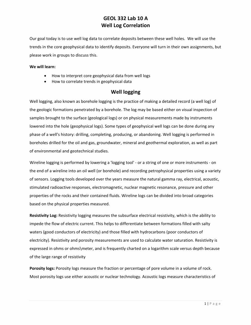
Part I. Correlation

For today’s lab, we will use well log data from wells drilled along Tompkins Hill, Humboldt County, CA.

These wells were drilled for hydrocarbon exploration in the 1960s. We will correlate packages of

sediments from well to well. We will make note of repeated section and differences in sedimentary unit

depth between wells.

We will correlate from hole to hole, the bases of sedimentary sequences. Use a pencil for your

correlations as you will be changing them as you work through this assignment. The well logs are from

wells located in the region below. Tape the well logs to the larger piece of paper and draw your

correlation lines on the larger piece of paper. The following information may help you select the

arrangement of the well logs (consider elevation and spatial location). Label some of the sedimentary

units that you correlate, using alphabetical letters, starting with A at the top.

Well ID Elevation

(ft.) Depth at Top of

Log (ft.) Location (Township/Range)

HE 5 764 2080 2564' S / 50' E from NW corner of Section 22

HE 7 613 1980 1629' N / 353' W from SE corner of Section 23

HE 8 484 1670 981' N / 2368' E from SW corner of Section 23

HE 10 575 1330 2200' S / 2650' E from NW corner of Section 23

GEOL 332 Lab 10 B Turbidite Correlation

1 | P a g e

Our goal today is to use geophysical data collected from sediment cores to correlate deposits between

these sediment cores. We will use the trends in the core geophysical data to identify turbidites with

similar trends. Everyone will turn in their own assignments, but please work in groups to discuss this.

We will learn:

How to interpret core geophysical data from turbidite stratigraphy

How to correlate trends in geophysical data

Core samples are collected on land and at sea by the hydrocarbon, mining and construction industries,

as well as by the military and by paleoseismologists. For academia they are now an essential part of

climatic research. The cores come as soft sediment encased in plastic sleeves. They can yield information

about the properties of rock or sedimentary strata. These geophysical properties can be used as proxies

for different parameter that might be useful for industry. The hydrocarbon industry, for example, needs

accurate data on the porosity, grain size, and correlation parameters to surrounding geology, whereas

the construction industry and the military may be interested in geotechnical properties such as P‐wave

velocities, density and water content. The range of parameters that can be measured includes P‐wave

velocity, gamma density, magnetic susceptibility, electrical resistivity, color line‐scan imaging, X‐ray

fluorescence, color spectrophotometry, and natural gamma spectrometry. Sediment cores may also be

analyzed using Computed Tomographic X‐Rays, resulting in CT‐scans (3‐D X‐Rays). Line‐scans of the CT

data can provide an independent view of density. Core data can be correlated by looking for matching

sequences in these parameters (Figure 1). Figure 2 shows the region from where the cores in Figure 1

were collected.

For today’s lab, we will use core log data from sediment cores collected offshore of Oregon. These cores

were initially collected to disprove the results of a paper published by Adams (1990), who concluded

that turbidites cored in the 1960s were initially triggered by Cascadia subduction zone earthquakes.

Unfortunately for the scientists in 1999 and 2002, they were unable to disprove Adams (1990).

Paleoseismologists use integrated stratigraphic correlation techniques, including visual lithostratigraphic

description (color, texture, and structure, etc.), CT image analysis, and lithostratigraphic log correlation

of Multi Sensor Core Logging (MSCL) geophysical data (Fukuma, 1998; Karlin et al., 2004; Abdeldayem et

al., 2004; St‐Onge et al., 2004; Hagstrum et al., 2004; Waldmann et al., 2011) to correlate turbidites

based on the turbidite “architecture” (Amy and Talling, 2006). Stratigraphic correlation using

geophysical signatures representing vertical turbidite structure is a primary tool for testing individual


2 | P a g e

deposits for their areal extent, a significant part of the criteria used to discriminate seismoturbidites

from other possible types. A positive correlation, regardless of the originating details, is indicative of a

co‐genetic origin. Down‐core geophysical properties for individual turbidites are reflections of the

vertical grain size distribution of the bed (Kneller and McCaffrey, 2003; Amy et al., 2005; Karlin and Seitz,

2007; Goldfinger et al., 2012). Lithostratigraphic correlation techniques have been used to correlate

stratigraphic units since the 1960’s (Prell, 1986; Lovlie and Van Veen, 1995). In detail these “fingerprints”

represent the time‐history of deposition of the turbidite and, in several cases linked to plate boundary

earthquakes, have been shown to correlate between independent sites separated by large distances and

depositional settings (Goldfinger et al., 2008, 2013). The turbidite itself is commonly composed of single

or multiple coarse fraction fining upward stacked units termed “pulses.” The rarity of a fine tail (Bouma

Td and Te; Bouma, 1962) or subsequent hemipelagic sediment between pulses indicates there is

commonly little or no temporal separation between units. The lack of temporal separation of the pulses

in Cascadia has been inferred to represent deposition over minutes to hours, so most likely represent

sub‐units of a single turbidite (Goldfinger et al., 2012).

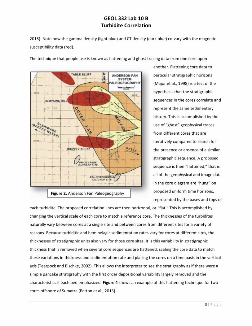
Figure 1. Correlation Diagram for Tertiary Anderson Fan sands. These turbidite sand deposits are found in the wells drilled in the Table Bluff, Thompkins Hill, and Grizzly Bluff regions, as well as found in outcrop al the Price Creek and Scotia sites.

Density and magnetic susceptibility tend to co‐vary with particle size; larger particles and magnetic

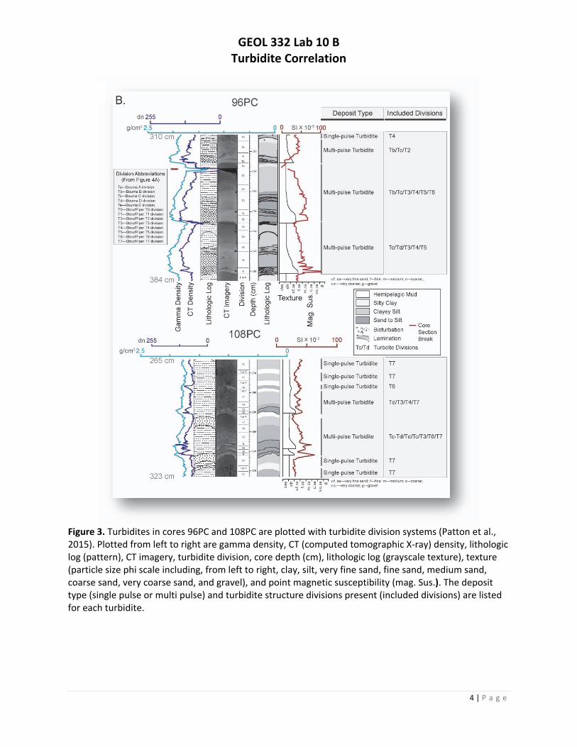
minerals are generally denser (Thompson and Morton, 1979). Figure 3 shows core geophysical data for

sections from cores 96PC and 108PC, collected in the deep sea offshore of Sumatra (Patton et al., 2013,


3 | P a g e

2015). Note how the gamma density (light blue) and CT density (dark blue) co‐vary with the magnetic

susceptibility data (red).

The technique that people use is known as flattening and ghost tracing data from one core upon

another. Flattening core data to

particular stratigraphic horizons

(Major et al., 1998) is a test of the

hypothesis that the stratigraphic

sequences in the cores correlate and

represent the same sedimentary

history. This is accomplished by the

use of “ghost” geophysical traces

from different cores that are

iteratively compared to search for

the presence or absence of a similar

stratigraphic sequence. A proposed

sequence is then “flattened,” that is

all of the geophysical and image data

in the core diagram are “hung” on

proposed uniform time horizons,

represented by the bases and tops of

each turbidite. The proposed correlation lines are then horizontal, or “flat.” This is accomplished by

changing the vertical scale of each core to match a reference core. The thicknesses of the turbidites

naturally vary between cores at a single site and between cores from different sites for a variety of

reasons. Because turbiditic and hemipelagic sedimentation rates vary for cores at different sites, the

thicknesses of stratigraphic units also vary for those core sites. It is this variability in stratigraphic

thickness that is removed when several core sequences are flattened, scaling the core data to match

these variations in thickness and sedimentation rate and placing the cores on a time basis in the vertical

axis (Tearpock and Bischke, 2002). This allows the interpreter to see the stratigraphy as if there were a

simple pancake stratigraphy with the first order depositional variability largely removed and the

characteristics if each bed emphasized. Figure 4 shows an example of this flattening technique for two

cores offshore of Sumatra (Patton et al., 2013).

Figure 2. Anderson Fan Paleogeography


4 | P a g e

Figure 3. Turbidites in cores 96PC and 108PC are plotted with turbidite division systems (Patton et al., 2015). Plotted from left to right are gamma density, CT (computed tomographic X‐ray) density, lithologic log (pattern), CT imagery, turbidite division, core depth (cm), lithologic log (grayscale texture), texture (particle size phi scale including, from left to right, clay, silt, very fine sand, fine sand, medium sand, coarse sand, very coarse sand, and gravel), and point magnetic susceptibility (mag. Sus.). The deposit type (single pulse or multi pulse) and turbidite structure divisions present (included divisions) are listed for each turbidite.


5 | P a g e

Figure 4. Correlation of sedimentary units using standard stratigraphic correlation techniques between cores RR0705‐55PC and RR0705‐57PC. A. Bathymetric map with cores plotted as brown dots and depth contours with 500 m spacing. Cores 55PC and 57 PC are located in the trench approximately 120 km from each other. B. Stratigraphic correlations between these cores using lithology, CT, and geophysical properties. Multi Sensor Core Log (MSCL) data are plotted beside RGB imagery and CT imagery that displays lower density material in darker grey and higher density material in lighter grey. Gamma density, CT density, and point magnetic susceptibility are plotted left to right as light blue, dark blue, and dark red. The certainty of any individual correlation is ranked and designated by line symbology. C. MSCL data for core 57PC is “flattened” to stratigraphic horizons in core 55PC on the left, and 55PC is flattened to 57PC on the right. The core data being flattened is transparent and plotted on the outside of the core data they are being flattened to. The un‐flattened core data are scaled at the same vertical scale as in B.


6 | P a g e

Part II. Correlation

We will correlate from core to core, the bases of turbidites. First we will correlate cores with no

numerical age control from cores collected in the western Atlantic Ocean. Then we will correlate two

cores that each have radiocarbon age estimates for the sediment underlying the turbidites. Sequentially

number the turbidites that you have correlated in each correlation figure, beginning with #1 for the

uppermost turbidite.

A. Antilles Correlation

We will correlate two pairs of cores from the Lesser Antilles, a magmatic arc related to subduction of the

Atlantic plate beneath the Caribbean plate. These cores were collected while I was at sea this summer

on the Poquois Pas?, a French research vessel. These core pairs are in sedimentary basins near the base

of the continental slope northeast of Guadeloupe (Figure 5). Correlate the bases of turbidites. Do as

many as you can.

Figure 5. Map of core sites in the Lesser Antilles. Depth contours are in blue. The city Pointe a Pitre is located at the white dot labeled PTP. Cores 2 and 12 are located really close to each other.

B. Cascadia Correlation

Now we will correlate one core pair from core data from two different sedimentological settings (one

core is from the base of a submarine canyon and one is at the base of a piggy back basin ridge along the

continental slope). Both of these cores are from the northeast Pacific Ocean and were used to develop


7 | P a g e

the earthquake chronology along the southern and central Cascadia subduction zone (Goldfinger et al.,

2012). We will use the radiocarbon ages as a first order control for our correlations. Note that there may

be errors beyond the analytical errors listed in the figure (i.e. the age may not best represent the

sediment sampled in the core; e.g. the sediment may be older or be younger than the radiocarbon age).

Use a pencil for your correlations as you will be changing them as you work through this assignment.

Correlate the bases of turbidites. Do as many as you can.

References:

Abdeldayem, A.L., Ikehara, K., Yamazaki, T., 2004. Flow path of the 1993 Hokkaido‐Nansei‐Oki earthquake seismoturbidite, southern

margin of the Japan sea north basin, inferred from anisotropy of magnetic susceptibility: Geophysical Journal International, v. 157, p.

15‐24, doi: 10.1111/j.1365‐246X.2004.02210.x.

Adams, J., 1990. Paleoseismicity of the Cascadia subduction zone: Evidence from turbidites off the Oregon‐Washington Margin:

Tectonics, v. 9, p. 569‐584.

Amy, L.A., Talling, P.J., Peakall, J., Wynn, R.B., Thynne, R.G.A., 2005. Bed geometry used to test recognition criteria of turbidites and

(sandy) debrites: Sedimentary Geology, v. 179, p. 163‐174.

Amy, L.A., Talling, P.J., 2006. Anatomy of turbidites and linked debrites based on long distance (120 ∙ 30 km) bed correlation,

Marnoso Arenacea Formation, Northern Apennines, Italy: Sedimentology, v. 53, p. 161‐212.

Bouma, A.H., 1962. Sedimentology of Some Flysch Deposits. Elsevier Publishing, 168 p.

Fukuma, K., 1998. Origin and applications of whole‐core magnetic susceptibility of sediments and volcanic rocks from Leg 152.

Proceedings of the Ocean Drilling Program: Scientific Results, v. 152, p. 271‐280.

Goldfinger, C., Nelson, C.H., Johnson, J.E., 2003. Holocene Earthquake Records From the Cascadia Subduction Zone and Northern San

Andreas Fault Based on Precise Dating of Offshore Turbidites: Annual Reviews of Earth and Planetary Sciences, v. 31, p. 555‐577.

Goldfinger, C., Nelson, C.H., Morey, A., Johnson, J.E., Gutierrez‐Pastor, J., Eriksson, A.T., Karabanov, E., Patton, J., Gràcia, E., Enkin, R.,

Dallimore, A., Dunhill, G., and Vallier, T., 2012. Turbidite Event History: Methods and Implications for Holocene Paleoseismicity of

the Cascadia Subduction Zone, USGS Professional Paper # 178. U.S. Geological Survey, Reston, VA.

Goldfinger, C., Morey, A., Black, B., Patton, J.R., 2013. Spatially Limited Mud Turbidites on the Cascadia Margin: Segmented

Earthquake Ruptures: Natural Hazards and Earth System Sciences, v. 13, p. 2,109‐2,146.

Hagstrum, J.T., Atwater, B.F., Sherrod, B.L., 2004. Paleomagnetic correlation of late Holocene earthquakes among estuaries in

Washington and Oregon: Geochemistry Geophysics Geosystems, v. 5, Q10001, doi: 10.1029/2004GC000736

Karlin, R.E., Holmes, M., Abella, S.E.B., Sylwester, R., 2004. Holocene landslides and a 3500‐year record of Pacific Northwest

earthquakes from sediments in Lake Washington: Geological Society of America Bulletin, v. 116, p. 94‐108.

Karlin, R., Seitz, G., 2007. A Basin Wide Record of Earthquakes at Lake Tahoe: Validation of the Earthquake Induced Turbidite Model

with Sediment Core Analysis: Collaborative Research with UNR and SDSU, Final Technical Report for 07HQGR0014 and 07HQGR0008,

U.S.G.S National Earthquake Hazards Reduction Program.

Kneller, B. C., and McCaffrey, W. D., 2003, The Interpretation of Vertical Sequences in Turbidite Beds: The Influence of Longitudinal

Flow Structure: Journal of Sedimentary Research, v. 73, no. 5, p. 706‐713.

Lovlie, R., Van Veen, P., 1995. Magnetic susceptibility of a 180 m sediment core: reliability of incremental sampling and evidence for

a relationship between susceptibility and gamma activity, in: Turner, P., Turner, A. (Eds.), Palaeomagnetic applications in

hydrocarbon exploration and production: Geological Society, London, Special Publication, v. 98, p. 259‐266.


8 | P a g e

Major, C. O., Pirmez, C., Goldberg, D., and Party, L. S., 1998. High‐resolution core‐log integration techniques: examples from the

Ocean Drilling Program, in Harvey, P. K., and Lovell, M. A., eds., Core‐Log Integration: London, England, Geological Society Special

Publication 136, p. 285‐295.

Patton, J. R., Goldfinger, C., Morey, A. E., Romsos, C., Black, B., Djadjadihardja, Y., Udrekh, 2013, Seismoturbidite Record as

Preserved at Core Sites at the Cascadia and Sumatra‐Andaman Subduction Zones: : The Offshore Search of Large Holocene

Earthquakes: Obergurgl, Austria, Natural Hazards and Earth System Sciences, 13, 833‐867.

Patton, J. R., Goldfinger, C., Morey, A. E., Ikehara, K., Romsos, C., Stoner, J., Djadjadihardja, Y., Udrekh, Ardhyastuti, S., Gaffar, E.Z.,

and Viscaino, A. 2015. A 6500 year earthquake history in the region of the 2004 Sumatra‐Andaman subduction zone Earthquake,

Geosphere, vol. 11, doi:10.1130/GES01066.1.

Prell, W.L., Imbrie, J., Martinson, D.G., Morley, J.J., Pisias, N.G., Shackleton, N.J., Streeter, H.F., 1986. Graphic Correlation Of Oxygen

Isotope Stratigraphy Application To The Late Quaternary: Paleoceanography, v. 1, p. 137‐162.

St‐Onge, G., Mulder, T., Piper, D.J.W., Hillaire‐Marcel, C., Stoner, J.S., 2004. Earthquake and flood‐induced turbidites in the Saguenay

Fjord (Québec): a Holocene paleoseismicity record: Quaternary Science Reviews, v. 23, p. 283‐294.

Tearpock, D. J., and Bischke, R. E., 2002. Applied subsurface geological mapping, Englewood Cliffs, NJ, Prentice‐Hall, Inc., 864 p.

Thompson, R., and Morton, D. J., 1979. Magnetic Susceptibility and Particle‐Size Distribution in Recent Sediments of the Loch

Lomond Drainage Basin, Scotland: Journal of Sedimentary Petrology, v. 49, no. 3, p. 801‐812.

Waldmann, N., Anselmetti, F.S., Ariztegui, D., Austin Jr., J.A., Pirouz, M., Moy, C.M., Dunbar, R.B., 2011. Holocene mass‐wasting

events in Lago Fagnano, Tierra del Fuego (54˚S): implications for paleoseismicity of the Magallanes‐Fagnano transform fault: Basin

Research, v. 23, p. 171‐190.

GEOL 332 Lab 10 Stratigraphic Correlation

Page | 1

Name: _____________________________________________ Date: _______________

Team Name: ___________________________ Team Members: ________________________________

____________________________________________________________________________________

Part III. Report

Please submit your correlation diagrams for Lab 10 A and Lab 10 B, along with a 3 page report that

summarizes your findings. Please be as scientific as you can. This report and correlation diagrams are

due in two weeks. Work on this project and report as a group, but everyone must submit their own

report and correlation diagrams.

Introduction:

Describe what this lab is about.

Mention why this method is used for hydrocarbon exploration. You may want to do some online research about this.

Mention why this method is used for submarine paleoseismology.

Methods:

For Lab 10 A, in your own words, describe what well log properties are, what they might be used as proxies for in the sediment cores, and the correlation methods used in this lab. You might want to do additional research about well log data.

For Lab 10 B, in your own words, describe what core geophysical properties are, what they might be used as proxies for in the sediment cores, and the correlation methods used in this lab.

Results:

For Lab 10 A, list the number of sedimentary packages that you were able to correlate. State whether these are sand or shale deposits. If you can quantify this, mention the number of sand and the number of shale units (or give a percentage).

For lab 10 B, list the number of turbidites that you were able to correlate in each correlation diagram.

Discussion:

This results section should provide the basis for an interpretation of the geologic history recorded in the sediments collected in these cores.

Based on your correlations, what can you say about the sedimentary history found in these cores? Be bold in your interpretations.

Conclusion:

A summary of your report.

GEOL 332 Lab 10 A Well Log Correlation Well logging...Well logging Well logging, also known as borehole logging is the practice of making a detailed record (a well log) of ... GEOL

Documents