Geography and macroeconomics: New data and … · Geography and macroeconomics: New data and new findings ... this focus is sensible for a discipline like economics, ... geography

Geography and macroeconomics: New dataand new findingsWilliam D. Nordhaus*

Yale University, 28 Hillhouse Avenue, New Haven, CT 06520-8268

This contribution is part of the special series of Inaugural Articles by members of the National Academy of Sciences elected on May 1, 2001.

Contributed by William D. Nordhaus, December 2, 2005

The linkage between economic activity and geography is obvious:Populations cluster mainly on coasts and rarely on ice sheets. Paststudies of the relationships between economic activity and geog-raphy have been hampered by limited spatial data on economicactivity. The present study introduces data on global economicactivity, the G-Econ database, which measures economic activityfor all large countries, measured at a 1° latitude by 1° longitudescale. The methodologies for the study are described. Three appli-cations of the data are investigated. First, the puzzling ‘‘climate-output reversal’’ is detected, whereby the relationship betweentemperature and output is negative when measured on a percapita basis and strongly positive on a per area basis. Second, thedatabase allows better resolution of the impact of geographicattributes on African poverty, finding geography is an importantsource of income differences relative to high-income regions.Finally, we use the G-Econ data to provide estimates of theeconomic impact of greenhouse warming, with larger estimates ofwarming damages than past studies.

economic growth � development � climate change

The linkage between economic activity and geography is obviousto most people: populations cluster mainly on coasts and rarely

on ice sheets. Yet, modern macroeconomics and growth economicsgenerally ignore geographic factors such as climate, proximity towater, soils, tropical pests, and permafrost. This inaugural essayexamines this intellectual division, presents data on geographicallybased economic activity, and examines some of the major relation-ships between macroeconomic activity and geographic measures. Afull description of the data and methods can be found at the projectweb site (http:��gecon.yale.edu).

Why has macroeconomics generally ignored geography? As willbe discussed in subsequent sections, three factors have prevented athorough integration of geographic factors into macroeconomicanalysis. First, economic growth theory has emphasized the role ofendogenous and policy factors, such as capital formation, educa-tion, and technology, rather than exogenous factors such as geog-raphy or even population. Although natural resources (particularlyland and minerals) have been featured in some studies, climate,soils, tropical diseases, and similar ‘‘unchanging’’ factors havetypically been omitted from modern economic growth analysis.

Second, studies of the impact of geography on economic activityhave emphasized the level or growth in per capita output. Althoughthis focus is sensible for a discipline like economics, which focuseson national economic policies and living standards, it is difficult tocapture time-invariant geographic factors in such studies. To sep-arate out geographic factors, this study examines areal density ofoutput and per capita output. We will see that shifting the measuredramatically changes the estimated effects of geography on eco-nomic activity.

Third, most measures of economic activity have been time seriesor panels measured at the level of the country, which provide �100observations at enormously different geographic scales. The dataset presented here (GECON 1.1), which measures output with aresolution of 1° latitude by 1° longitude, covers 25,572 terrestrialgrid cells. Such an increase in resolution is analogous to pictures

from the Hubble telescope, which provide clear and crisp answersto many previously difficult and fuzzily answered questions.

The change in emphasis proposed here has an enormous effecton the estimated impact of geographic attributes on economicactivity. The G-Econ database (described in detail in the secondpart of this article) can be useful not only for economists interestedin spatial economics but equally for environmental scientists look-ing to link their satellite and other geographically based data witheconomic data.

I begin with a brief survey of the role of geographic factors ineconomic analysis and empirical work. In this survey, I will discussmainly macroeconomics, and it must be emphasized that theseremarks present a highly condensed view of studies that relate toglobal economic processes. The vast and impressive literature ingeography and regional economics is largely outside the scope ofthis study.

It will be useful to state what I mean by ‘‘geographical’’ factors(or, better, geophysical factors studied in ‘‘physical geography’’).These physical attributes are tied to specific locations. They may benonstochastic on the relevant time scale (such as latitude, distancefrom coastlines, or elevation) or they may be stochastic with slowlymoving means and variability (such as climate or soils). One of thecritical features of the present approach is that geographic factorsare statistically exogenous in the sense that they cause, but to a firstapproximation are not caused by, economic and other socialvariables. For our purposes, we omit most environmental andendogenous geographic variables, such as pollution, land use, andthe natural-resource content of trade or output. Although thesefactors are of critical importance for many purposes, the focus hereis on exogenous and large-scale factors that are largely unaffectedby human activities on decadal time scales.

In reflecting on the wealth of nations, early economists assumedthat climate was one of the prime determinants of national differ-ences. In societies where most of the population lived on farms, thispresumption was probably correct. Earlier civilizations, such asthose investigated in Landes’s history of economic growth (1) orDiamond’s analysis of societal collapses (2), were highly dependenton local resources and climatic conditions and less able to specializeand trade than most economies today.

However, one of the major factors in economic development hasbeen the movement from climatic-sensitive farming and into cli-mate-insensitive manufacturing and services. In 1820, 72% of U.S.employment was on farms, whereas by 2004, the share was down to1.2%. Many studies suggest that the market economy in thedeveloped world is relatively insensitive to moderate and gradualchanges in climate or similar geographic conditions (see below).

Current theories and empirical studies of economic growth todaygive short shrift to climate as the basis for the differences in the

Conflict of interest statement: No conflicts declared.

Freely available online through the PNAS open access option.

Abbreviation: GCP, gross cell product.

*E-mail: [email protected].

© 2006 by The National Academy of Sciences of the USA

3510–3517 � PNAS � March 7, 2006 � vol. 103 � no. 10 www.pnas.org�cgi�doi�10.1073�pnas.0509842103

wealth of nations. A review of a handful of textbooks on economicdevelopment shows that climate is confined to a few lines inhundreds of pages. (Exceptions are ref. 3 and more recent workdiscussed later.) The modern view of economic growth presentsdevelopment as an engine fueled by capital, labor, and technology;sometimes, mineral resources are included, but only with a majorstretch of interpretation would we equate resources with geo-graphic attributes. The recent wave of studies investigating inter-national differences in productivity has generally omitted climate asa determining variable.

Over the last decade, economists have begun to introducegeography into studies of economic growth and development. Oneearly set of studies by Hall and Jones (4) investigated the reasonsfor the enormous diversity of per capita incomes across nations.Their main hypothesis was that average output differences acrossnations are primarily determined by institutions and governmentpolicies. In examining statistically exogenous instruments, theyfound that geography (measured as distance from the equator) wasamong the most significant variables behind differences in percapita output by country. They speculated that location affectseconomic success because of patterns of human settlements, whichinfluence institutions.

The study of economic geography has been revitalized by thework of Sachs and his colleagues (5, 6). The major thrust of thiswork is to understand the economic problems of tropical Africa.They examine geographic factors such as the percent of the landarea in the tropics as influencing growth. Their surprising conclu-sion is ‘‘Our statistical estimates, admittedly imprecise, actually giveapproximately two-thirds of the weight of Africa’s growth shortfallto the ‘noneconomic’ conditions, and only one-third to economicpolicy and institutions’’ (5). Other studies examine the role of‘‘landlockedness,’’ coastal settlements, and tropical diseases oneconomic activity (6).

The geographically based studies on Africa have come underheavy criticism for both technical and economic reasons. One set ofissues concerns the statistical ‘‘endogeneity’’ of the independentvariables. A second and more far-reaching criticism concerns therelative importance of institutions. Several studies argue (along thelines of Hall and Jones discussed above) that high incomes today arebest understood as determined by historical conditions in whichgeography led to settlement patterns that were favorable to goodinstitutions (such as British settlement in North America), and thenthat good institutions led to high incomes (7). Although thesestudies are not the last word on the subject, a casual look at East andWest Germany, North and South Korea, and Baja and AltaCalifornia surely suggests the importance of institutions in eco-nomic growth.

Existing studies serve many useful purposes, but they have threedistinct shortcomings for determining the impact of geographicattributes on economic activity, all of which are remedied by thepresent data set. First, virtually all studies focus on national data. Ifinstitutions are indeed a key ingredient in economic growth, thenit would be very difficult to sort out geographic from nationalinfluences without disaggregating below the national level. Thegridded data used here overcome this obstacle by employing almost20,000 terrestrial observations (hence, many per nation) as com-pared to the 100 or so national observations customarily used in thestudies just reviewed.

Second, the analysis here is primarily concerned with the geo-graphic intensity of economic activity rather than the personalintensity of economic activity. In other words, it focuses on theintensity of economic activity per unit area rather than per capitaor per hour worked. Although geographic intensity may be lessinteresting for many policy purposes than the determinants of percapita income, the present approach places the emphasis clearly ongeography.

Third, virtually all prior studies have focused on proxies forgeographic variables rather than those that are intrinsically impor-

tant. Distance from the equator and percent area in the tropics, forexample, have no intrinsic economic significance. One of theadvantages of using gridded data rather than national data is thatthey allow us to use a much richer set of geographic attributes. Mostof the important geographic data (including climate, location,distance from markets or seacoasts, and soils) are collated on ageographic basis rather than based on political boundaries. Thereis also an important interaction between the finer resolution of theeconomic data and the use of geographic data because, for manycountries, averages of most geographic variables (such as temper-ature or distance from seacoast) cover such a huge area that theyare virtually meaningless, whereas for most grid cells the averagescover a reasonably small area.

Methodology for Estimating Gross Cell ProductThe Concept of Gross Cell Product (GCP). The major statisticalcontribution of the present research program has been the devel-opment of ‘‘gridded output’’ data, or GCP. In this work, the ‘‘cell’’is the surface bounded by 1-degree latitude by 1-degree longitudecontours. A full description of the data and methods can be foundat the project web site (http:��gecon.yale.edu).

The globe contains 64,800 such grid cells; we provide outputestimates for 25,572 terrestrial cells. Of these terrestrial cells, 19,136cells are outside Antarctica, 17,433 have complete and minimum-quality data, and 14,859 have complete, minimum-quality data withnonzero population and output.

The grid cell is selected because it is the unit for which data,particularly on population, are most plentiful. It also is the mostconvenient for integrating with global environmental data. Addi-tionally, this coordinate system is (to a first approximation) statis-tically independent of economic data (which obviously is not thecase for political boundaries), and the elements are of (almost)uniform size except in polar regions. From a practical point of view,there is no alternative to a grid measurement system such as the oneused in the paper.

The conceptual basis of GCP is the same as that of gross domesticproduct and gross regional product as developed in the nationalincome and product accounts of major countries, except that thegeographic unit is the latitude-longitude grid cell. GCP is grossvalue added in a specific geographic region; gross value added isequal to total production of market goods and services in a regionless purchases from other businesses. GCP aggregates across allcells in a country to gross domestic product. We measure output inpurchasing-power-corrected 1995 U.S. dollars by using nationalaggregates estimated by the World Bank. We do not generallyadjust for purchasing-power differences within individual countries.The exception to this rule is that we make purchasing-poweradjustments for oil and mineral production in countries with a highproportion of output coming from these sources.

The general methodology for calculating GCP is the following:

GCP by grid cell � (population by grid cell)

� �per capita GCP by grid cell). [1]

The approach in Eq. 1 is particularly attractive because a teamof geographers and demographers has recently constructed adetailed set of population estimates by grid cell, the first term onthe right-hand side of Eq. 1.† Estimates of GCP, therefore,primarily require new estimates of per capita output by grid cell.

Methodologies for Estimating Per Capita GCP. The detail and accu-racy of economic and demographic data vary widely among coun-tries, and we have developed alternative methodologies dependingon the data availability and quality. The methodologies are de-

†The gridded population data are available online at http:��sedac.ciesin.columbia.edu�plue�gpw with full documentation in ref. 8 and updated in ref. 9.

Nordhaus PNAS � March 7, 2006 � vol. 103 � no. 10 � 3511

SUST

AIN

ABI

LITY

SCIE

NCE

INA

UG

URA

LA

RTIC

LE

scribed (http:��gecon.yale.edu; W.N., Q. Azam, D. Corderi, N. M.Victor, M. Mohammed, and A. Miltner, unpublished data), anddata for each country are also available upon request.

In developing the data and methods for the project, two differentattributes are central: the level of spatial disaggregation and thesource data used to construct the estimates of gross cell product. Interms of spatial disaggregation, there are usually three politicalsubdivisions: (i) national data, (ii) ‘‘state data’’ from the firstpolitical subdivision, and (iii) ‘‘province data’’ from the secondpolitical subdivision. We use the lowest political subdivision forwhich data are available, although different levels are sometimescombined.

There are four major sources of the economic data: (i) grossregional product (such as gross state product for the United States),(ii) regional income by industry (such as labor income by industryand counties or provinces for the United States and Canada), (iii)regional employment by industry (such as detailed employment byindustry and region for Egypt), and (iv) regional urban and ruralpopulation or employment along with aggregate sectoral data onagricultural and nonagricultural incomes (used for African coun-tries such as Niger). For each country, we combine one or more ofthe four data sets at one or more regional levels.

Specific Methodologies. Some examples illustrate the variety ofmethodologies. (i) For the United States, government estimates areavailable for gross state product for 50 states. We use detailed dataon labor income by industry for 3,100 counties to develop per capitagross county product. We then apply spatial rescaling describedbelow to convert the county data to the 1,369 terrestrial grid cellsfor the United States. We would judge these estimates to be highlyreliable. A similar approach was used for Canada, the EuropeanUnion, and Brazil. (ii) For most other high-income countries, weuse gross regional product by first political subdivision (such asoblasts for the Russian Federation). For small- or medium-sizedcountries (Argentina), this approach will be relatively reliable,whereas for large countries (Russia) the regions are sometimes verylarge and the spatial resolution is consequently poor. (iii) For manymiddle-income countries, such as Egypt, we have data from recentcensuses, which collect data on employment by region and industry.We then use these data along with national accounts data onnational output by industry to estimate output by region andindustry and then aggregate these data across industries to obtainestimates of gross regional product. (iv) For Nigeria and many of thelowest-income countries, we have no regional economic data. Inthese cases, we combine population censuses on rural and urbanpopulations with national employment and output data to estimateoutput per capita by region. For these countries, because of thesparse economic data and limited regional data, estimates of GCPare less accurate than those for high-income countries.

Spatial Rescaling. The data on output and per capita output areestimated by political boundaries. To create gridded data, we needto transform the data to geographic boundaries. I call this process‘‘spatial rescaling,’’ although it goes by many names in quantitativegeography such as ‘‘the modifiable areal unit problem,’’ ‘‘cross-areaaggregation,’’ or ‘‘areal interpolation’’ (10–12). Spatial rescalingarises in a number of different contexts and requires inferring thedistribution of the data in one set of spatial aggregates based on thedistribution in another set of spatial aggregates, where neither is asubset of the other. The scaling problem arises here because alleconomic data are published by using political boundaries, andthese data need to be converted to geographic boundaries.

Having reviewed alternative approaches and done some simu-lations with economic data, we settled on the ‘‘proportional allo-cation’’ rule (details available upon request). The first step is todivide each grid cell into ‘‘subgrid cells,’’ each of which belongsuniquely to the smallest available political unit (call them ‘‘prov-inces’’). The next step is to collect or estimate per capita output for

each province. Third, the proportional allocation rule assumes thatper capita output is uniformly distributed in each province and thatpopulation is uniformly distributed in each grid cell. Based on theseassumptions, we can calculate a tentative estimate of output foreach subgrid cell as the product of the subgrid cell area times thepopulation density of the grid cell times the per capita output of theprovince. We next calculate the GCP as the sum of the outputs ofeach subgrid cell. The final step is to adjust the GCPs to conformto the totals for the province and the country.

This approach is data-intensive and computationally burden-some because it requires estimating the fraction of each grid cellbelonging to each province and estimating the economic data foreach of the provinces. Calculations indicate that there are signifi-cant gains in accuracy from disaggregating. For the United States,using actual county data, we estimate that disaggregating from thenational average to counties decreases the root mean squared errorof the cell average by a factor of 5.

Impact of Geography, Climate, and Other GeographicActivities on Economic ActivityThis final section presents some results of analyzing the patterns ofeconomic activity by using the new G-Econ data set. This study isnot meant to be a comprehensive analysis, which must awaitintegrating the data with a further geographic attributes and timeseries on spatial economic data. Moreover, at this point, we areprimarily examining basic patterns and reduced-form estimates;future work should focus on structural estimates of the majorvariables.

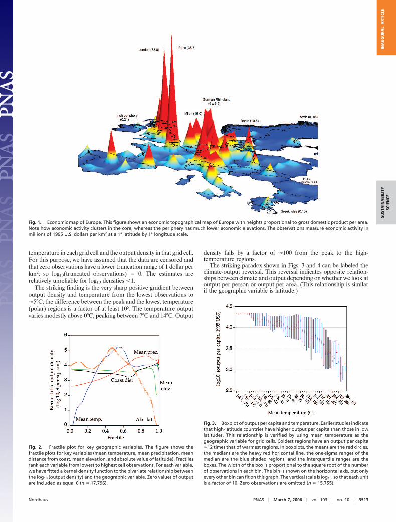
An Economic Map of Europe. Fig. 1 shows an economic contour mapof Europe, with some important mountains and lowlands marked.Unlike familiar contour maps, this one has height proportional tothe output density (output per square kilometer) in differentregions. The economic Mt. Everests are located along a core regionfrom southern England through northern Italy, whereas the pe-ripheral areas, particularly arctic Europe, are the economic low-lands. Maps for other countries are available upon request.

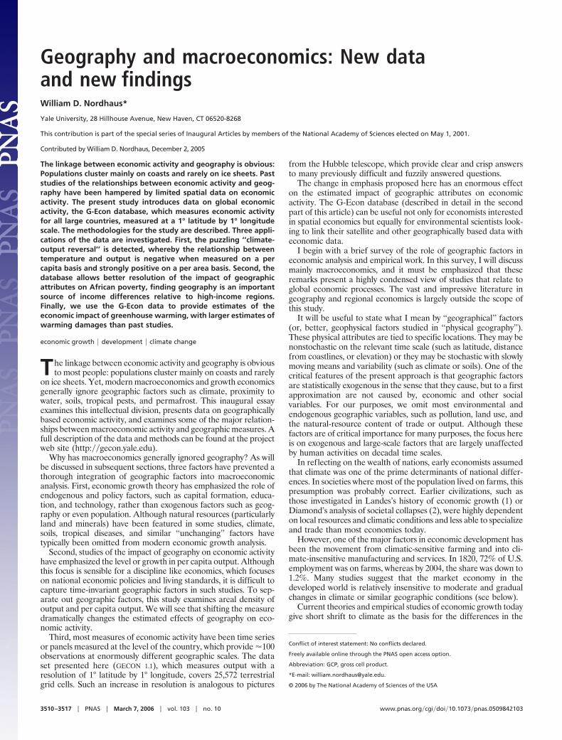
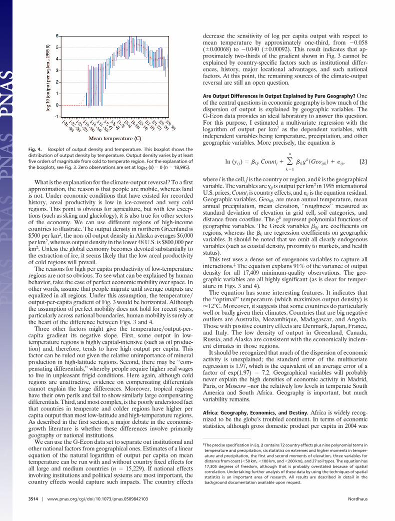
Fig. 2 shows fractile kernel plots of five major geographicvariables. A fractile plot first orders the variable from lowest tohighest observation. It then estimates a kernel density function orsmoothed nonlinear relationship between the fractile and thelogarithm (log10) of output density. For example, output densitydiffers by a factor of 105 from fractile trough to peak for meantemperature, whereas the difference for mean precipitation is 102

from trough to peak. Clearly, all geographic variables have majorsystematic impacts on economic activity. The relationships aredifficult to capture in a simple fashion because the impacts arehighly nonlinear.

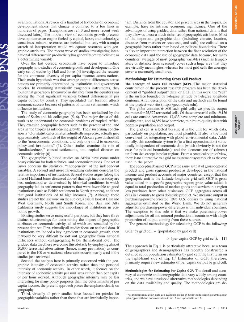
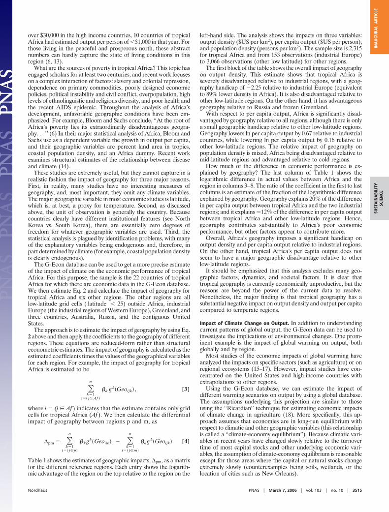
The Climate-Output Reversal. The first set of tests examines therelationship between economic activity and a limited set of geo-graphic activities, focusing primarily on climate. Many economicstudies have examined the relationship between geography andeconomic activity. One of the major findings is that output percapita rises with distance from the equator. Those studies have usedcountries as the unit of observation. Are the results confirmed whenthe unit of observation is refined to grid cells within countries?

Fig. 3 shows a ‘‘box plot’’ of the relationship between meantemperature in each grid cell and the output per capita in that gridcell. A box plot groups the observations in each bin and thenestimates several statistics for those observations; the differentstatistics are explained in the Fig. 3 legend. For this purpose, binshave a 2°C width (every second bin is shown on the bottom axis).Fig. 3 confirms the strong negative but highly nonlinear relationshipbetween temperature and per capita output.

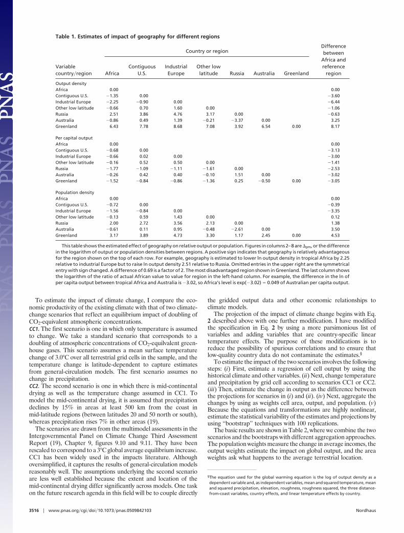
Although per capita output is a key economic variable, output perunit area is the key variable from a geographic and ecological pointof view. Fig. 4 shows a box plot of the relationship between mean

3512 � www.pnas.org�cgi�doi�10.1073�pnas.0509842103 Nordhaus

temperature in each grid cell and the output density in that grid cell.For this purpose, we have assumed that the data are censored andthat zero observations have a lower truncation range of 1 dollar perkm2, so log10(truncated observations) � 0. The estimates arerelatively unreliable for log10 densities �1.

The striking finding is the very sharp positive gradient betweenoutput density and temperature from the lowest observations to�5°C; the difference between the peak and the lowest temperature(polar) regions is a factor of at least 105. The temperature outputvaries modestly above 0°C, peaking between 7°C and 14°C. Output

density falls by a factor of �100 from the peak to the high-temperature regions.

The striking paradox shown in Figs. 3 and 4 can be labeled theclimate-output reversal. This reversal indicates opposite relation-ships between climate and output depending on whether we look atoutput per person or output per area. (This relationship is similarif the geographic variable is latitude.)

Fig. 2. Fractile plot for key geographic variables. The figure shows thefractile plots for key variables (mean temperature, mean precipitation, meandistance from coast, mean elevation, and absolute value of latitude). Fractilesrank each variable from lowest to highest cell observations. For each variable,we have fitted a kernel density function to the bivariate relationship betweenthe log10 (output density) and the geographic variable. Zero values of outputare included as equal 0 (n � 17,796).

Fig. 1. Economic map of Europe. This figure shows an economic topographical map of Europe with heights proportional to gross domestic product per area.Note how economic activity clusters in the core, whereas the periphery has much lower economic elevations. The observations measure economic activity inmillions of 1995 U.S. dollars per km2 at a 1° latitude by 1° longitude scale.

Fig. 3. Boxplot of output per capita and temperature. Earlier studies indicatethat high-latitude countries have higher output per capita than those in lowlatitudes. This relationship is verified by using mean temperature as thegeographic variable for grid cells. Coldest regions have an output per capita�12 times that of warmest regions. In boxplots, the means are the red circles,the medians are the heavy red horizontal line, the one-sigma ranges of themedian are the blue shaded regions, and the interquartile ranges are theboxes. The width of the box is proportional to the square root of the numberof observations in each bin. The bin is shown on the horizontal axis, but onlyevery other bin can fit on this graph. The vertical scale is log10, so that each unitis a factor of 10. Zero observations are omitted (n � 15,755).

Nordhaus PNAS � March 7, 2006 � vol. 103 � no. 10 � 3513

SUST

AIN

ABI

LITY

SCIE

NCE

INA

UG

URA

LA

RTIC

LE

What is the explanation for the climate-output reversal? To a firstapproximation, the reason is that people are mobile, whereas landis not. Under economic conditions that have existed for recordedhistory, areal productivity is low in ice-covered and very coldregions. This point is obvious for agriculture, but with few excep-tions (such as skiing and glaciology), it is also true for other sectorsof the economy. We can use different regions of high-incomecountries to illustrate. The output density in northern Greenland is$500 per km2, the non-oil output density in Alaska averages $6,000per km2, whereas output density in the lower 48 U.S. is $800,000 perkm2. Unless the global economy becomes devoted substantially tothe extraction of ice, it seems likely that the low areal productivityof cold regions will prevail.

The reasons for high per capita productivity of low-temperatureregions are not so obvious. To see what can be explained by humanbehavior, take the case of perfect economic mobility over space. Inother words, assume that people migrate until average outputs areequalized in all regions. Under this assumption, the temperature�output-per-capita gradient of Fig. 3 would be horizontal. Althoughthe assumption of perfect mobility does not hold for recent years,particularly across national boundaries, human mobility is surely atthe heart of the difference between Figs. 3 and 4.

Three other factors might give the temperature�output-per-capita gradient its negative slope. First, some output in low-temperature regions is highly capital-intensive (such as oil produc-tion) and, therefore, tends to have high output per capita. Thisfactor can be ruled out given the relative unimportance of mineralproduction in high-latitude regions. Second, there may be ‘‘com-pensating differentials,’’ whereby people require higher real wagesto live in unpleasant frigid conditions. Here again, although coldregions are unattractive, evidence on compensating differentialscannot explain the large differences. Moreover, tropical regionshave their own perils and fail to show similarly large compensatingdifferentials. Third, and most complex, is the poorly understood factthat countries in temperate and colder regions have higher percapita output than most low-latitude and high-temperature regions.As described in the first section, a major debate in the economic-growth literature is whether these differences involve primarilygeography or national institutions.

We can use the G-Econ data set to separate out institutional andother national factors from geographical ones. Estimates of a linearequation of the natural logarithm of output per capita on meantemperature can be run with and without country fixed effects forall large and medium countries (n � 15,229). If national effectsinvolving institutions and political systems are most important, thecountry effects would capture such impacts. The country effects

decrease the sensitivity of log per capita output with respect tomean temperature by approximately one-third, from �0.058(�0.00068) to �0.040 (�0.00092). This result indicates that ap-proximately two-thirds of the gradient shown in Fig. 3 cannot beexplained by country-specific factors such as institutional differ-ences, history, major locational advantages, and such nationalfactors. At this point, the remaining sources of the climate-outputreversal are still an open question.

Are Output Differences in Output Explained by Pure Geography? Oneof the central questions in economic geography is how much of thedispersion of output is explained by geographic variables. TheG-Econ data provides an ideal laboratory to answer this question.For this purpose, I estimated a multivariate regression with thelogarithm of output per km2 as the dependent variables, withindependent variables being temperature, precipitation, and othergeographic variables. More precisely, the equation is

ln (yi j) � �0j Countj � �k�1

n

�k gk�Geoijk� � � ij, [2]

where i is the cell, j is the country or region, and k is the geographicalvariable. The variables are yij is output per km2 in 1995 internationalU.S. prices, Countj is country effects, and �ij is the equation residual.Geographic variables, Geoijk, are mean annual temperature, meanannual precipitation, mean elevation, ‘‘roughness’’ measured asstandard deviation of elevation in grid cell, soil categories, anddistance from coastline. The gk represent polynomial functions ofgeographic variables. The Greek variables �0 j are coefficients onregions, whereas the �k are regression coefficients on geographicvariables. It should be noted that we omit all clearly endogenousvariables (such as coastal density, proximity to markets, and healthstatus).

This test uses a dense set of exogenous variables to capture allinteractions.‡ The equation explains 91% of the variance of outputdensity for all 17,409 minimum-quality observations. The geo-graphic variables are all highly significant (as is clear for temper-ature in Figs. 3 and 4).

The equation has some interesting features. It indicates thatthe ‘‘optimal’’ temperature (which maximizes output density) is�12°C. Moreover, it suggests that some countries do particularlywell or badly given their climates. Countries that are big negativeoutliers are Australia, Mozambique, Madagascar, and Angola.Those with positive country effects are Denmark, Japan, France,and Italy. The low density of output in Greenland, Canada,Russia, and Alaska are consistent with the economically inclem-ent climates in those regions.

It should be recognized that much of the dispersion of economicactivity is unexplained; the standard error of the multivariateregression is 1.97, which is the equivalent of an average error of afactor of exp(1.97) � 7.2. Geographical variables will probablynever explain the high densities of economic activity in Madrid,Paris, or Moscow –nor the relatively low levels in temperate SouthAmerica and South Africa. Geography is important, but muchvariability remains.

Africa: Geography, Economics, and Destiny. Africa is widely recog-nized to be the globe’s troubled continent. In terms of economicstatistics, although gross domestic product per capita in 2004 was

‡The precise specification in Eq. 2 contains 72 country effects plus nine polynomial terms intemperature and precipitation, six statistics on extremes and higher moments in temper-ature and precipitation, the first and second moments of elevation, three variables fordistance from coast (�50 km, �100 km, and �200 km), and 27 soil types. The equation has17,305 degrees of freedom, although that is probably overstated because of spatialcorrelation. Undertaking further analysis of these data by using the techniques of spatialstatistics is an important area of research. All results are described in detail in thebackground documentation available upon request.

Fig. 4. Boxplot of output density and temperature. This boxplot shows thedistribution of output density by temperature. Output density varies by at leastfive orders of magnitude from cold to temperate region. For the explanation ofthe boxplots, see Fig. 3. Zero observations are set at log10 (x) � 0 (n � 18,995).

3514 � www.pnas.org�cgi�doi�10.1073�pnas.0509842103 Nordhaus

over $30,000 in the high income countries, 10 countries of tropicalAfrica had estimated output per person of �$1,000 in that year. Forthose living in the peaceful and prosperous north, these abstractnumbers can hardly capture the state of living conditions in thisregion (6, 13).

What are the sources of poverty in tropical Africa? This topic hasengaged scholars for at least two centuries, and recent work focuseson a complex interaction of factors: slavery and colonial repression,dependence on primary commodities, poorly designed economicpolicies, political instability and civil conflict, overpopulation, highlevels of ethnolinguistic and religious diversity, and poor health andthe recent AIDS epidemic. Throughout the analysis of Africa’sdevelopment, unfavorable geographic conditions have been em-phasized. For example, Bloom and Sachs conclude, ‘‘At the root ofAfrica’s poverty lies its extraordinarily disadvantageous geogra-phy. . . ’’ (6) In their major statistical analysis of Africa, Bloom andSachs use as a dependent variable the growth in output per capita,and their geographic variables are percent land area in tropics,coastal population density, and an Africa dummy. Recent workexamines structural estimates of the relationship between diseaseand climate (14).

These studies are extremely useful, but they cannot capture in arealistic fashion the impact of geography for three major reasons.First, in reality, many studies have no interesting measures ofgeography, and, most important, they omit any climate variables.The major geographic variable in most economic studies is latitude,which is, at best, a proxy for temperature. Second, as discussedabove, the unit of observation is generally the country. Becausecountries clearly have different institutional features (see NorthKorea vs. South Korea), there are essentially zero degrees offreedom for whatever geographic variables are used. Third, thestatistical analysis is plagued by identification problems, with manyof the explanatory variables being endogenous and, therefore, inpart determined by climate (for example, coastal population densityis clearly endogenous).

The G-Econ database can be used to get a more precise estimateof the impact of climate on the economic performance of tropicalAfrica. For this purpose, the sample is the 22 countries of tropicalAfrica for which there are economic data in the G-Econ database.We then estimate Eq. 2 and calculate the impact of geography fortropical Africa and six other regions. The other regions are alllow-latitude grid cells ( latitude � 25) outside Africa, industrialEurope (the industrial regions of Western Europe), Greenland, andthree countries, Australia, Russia, and the contiguous UnitedStates.

The approach is to estimate the impact of geography by using Eq.2 above and then apply the coefficients to the geography of differentregions. These equations are reduced-form rather than structuraleconometric estimates. The impact of geography is calculated as theestimated coefficients times the values of the geographical variablesfor each region. For example, the impact of geography for tropicalAfrica is estimated to be

�k�1

i�� j� Af �

n

�k g k�Geoijk� , [3]

where i � (j � Af ) indicates that the estimate contains only gridcells for tropical Africa (Af ). We then calculate the differentialimpact of geography between regions p and m, as

�pm � �k�1

i�� j�p�

n

�k gk�Geoijk� � �k�1

i�� j�m�

n

�k g k�Geoijk�. [4]

Table 1 shows the estimates of geographic impacts, �pm, as a matrixfor the different reference regions. Each entry shows the logarith-mic advantage of the region on the top relative to the region on the

left-hand side. The analysis shows the impacts on three variables:output density ($US per km2), per capita output ($US per person),and population density (persons per km2). The sample size is 2,315for tropical Africa and from 153 observations (industrial Europe)to 3,066 observations (other low latitude) for other regions.

The first block of the table shows the overall impact of geographyon output density. This estimate shows that tropical Africa isseverely disadvantaged relative to industrial regions, with a geog-raphy handicap of �2.25 relative to industrial Europe (equivalentto 89% lower density in Africa). It is also disadvantaged relative toother low-latitude regions. On the other hand, it has advantageousgeography relative to Russia and frozen Greenland.

With respect to per capita output, Africa is significantly disad-vantaged by geography relative to all regions, although there is onlya small geographic handicap relative to other low-latitude regions.Geography lowers ln per capita output by 0.67 relative to industrialcountries, while lowering ln per capita output by 0.16 relative toother low-latitude regions. The relative impact of geography onpopulation density is mixed, Africa being disadvantaged relative tomid-latitude regions and advantaged relative to cold regions.

How much of the difference in economic performance is ex-plained by geography? The last column of Table 1 shows thelogarithmic difference in actual values between Africa and theregion in columns 3–8. The ratio of the coefficient in the first to lastcolumns is an estimate of the fraction of the logarithmic differenceexplained by geography. Geography explains 20% of the differencein per capita output between tropical Africa and the two industrialregions; and it explains �12% of the difference in per capita outputbetween tropical Africa and other low-latitude regions. Hence,geography contributes substantially to Africa’s poor economicperformance, but other factors appear to contribute more.

Overall, Africa’s geography imposes a significant handicap onoutput density and per capita output relative to industrial regions.On the other hand, tropical Africa’s per capita output does notseem to have a major geographic disadvantage relative to otherlow-latitude regions.

It should be emphasized that this analysis excludes many geo-graphic factors, dynamics, and societal factors. It is clear thattropical geography is currently economically unproductive, but thereasons are beyond the power of the current data to resolve.Nonetheless, the major finding is that tropical geography has asubstantial negative impact on output density and output per capitacompared to temperate regions.

Impact of Climate Change on Output. In addition to understandingcurrent patterns of global output, the G-Econ data can be used toinvestigate the implications of environmental changes. One prom-inent example is the impact of global warming on output, bothglobally and by region.

Most studies of the economic impacts of global warming haveanalyzed the impacts on specific sectors (such as agriculture) or onregional ecosystems (15–17). However, impact studies have con-centrated on the United States and high-income countries withextrapolations to other regions.

Using the G-Econ database, we can estimate the impact ofdifferent warming scenarios on output by using a global database.The assumptions underlying this projection are similar to thoseusing the ‘‘Ricardian’’ technique for estimating economic impactsof climate change in agriculture (18). More specifically, this ap-proach assumes that economies are in long-run equilibrium withrespect to climatic and other geographic variables (this relationshipis called a ‘‘climate-economy equilibrium’’). Because climatic vari-ables in recent years have changed slowly relative to the turnovertime of most capital stocks and other underlying economic vari-ables, the assumption of climate-economy equilibrium is reasonableexcept for those areas where the capital or natural stocks changeextremely slowly (counterexamples being soils, wetlands, or thelocation of cities such as New Orleans).

Nordhaus PNAS � March 7, 2006 � vol. 103 � no. 10 � 3515

SUST

AIN

ABI

LITY

SCIE

NCE

INA

UG

URA

LA

RTIC

LE

To estimate the impact of climate change, I compare the eco-nomic productivity of the existing climate with that of two climate-change scenarios that reflect an equilibrium impact of doubling ofCO2-equivalent atmospheric concentrations.CC1. The first scenario is one in which only temperature is assumedto change. We take a standard scenario that corresponds to adoubling of atmospheric concentrations of CO2-equilvalent green-house gases. This scenario assumes a mean surface temperaturechange of 3.0°C over all terrestrial grid cells in the sample, and thetemperature change is latitude-dependent to capture estimatesfrom general-circulation models. The first scenario assumes nochange in precipitation.CC2. The second scenario is one in which there is mid-continentaldrying as well as the temperature change assumed in CC1. Tomodel the mid-continental drying, it is assumed that precipitationdeclines by 15% in areas at least 500 km from the coast inmid-latitude regions (between latitudes 20 and 50 north or south),whereas precipitation rises 7% in other areas (19).

The scenarios are drawn from the multimodel assessments in theIntergovernmental Panel on Climate Change Third AssessmentReport (19), Chapter 9, figures 9.10 and 9.11. They have beenrescaled to correspond to a 3°C global average equilibrium increase.CC1 has been widely used in the impacts literature. Althoughoversimplified, it captures the results of general-circulation modelsreasonably well. The assumptions underlying the second scenarioare less well established because the extent and location of themid-continental drying differ significantly across models. One taskon the future research agenda in this field will be to couple directly

the gridded output data and other economic relationships toclimate models.

The projection of the impact of climate change begins with Eq.2 described above with one further modification. I have modifiedthe specification in Eq. 2 by using a more parsimonious list ofvariables and adding variables that are country-specific lineartemperature effects. The purpose of these modifications is toreduce the possibility of spurious correlations and to ensure thatlow-quality country data do not contaminate the estimates.§

To estimate the impact of the two scenarios involves the followingsteps: (i) First, estimate a regression of cell output by using thehistorical climate and other variables. (ii) Next, change temperatureand precipitation by grid cell according to scenarios CC1 or CC2.(iii) Then, estimate the change in output as the difference betweenthe projections for scenarios in (i) and (ii). (iv) Next, aggregate thechanges by using as weights cell area, output, and population. (v)Because the equations and transformations are highly nonlinear,estimate the statistical variability of the estimates and projections byusing ‘‘bootstrap’’ techniques with 100 replications.

The basic results are shown in Table 2, where we combine the twoscenarios and the bootstraps with different aggregation approaches.The population weights measure the change in average incomes, theoutput weights estimate the impact on global output, and the areaweights ask what happens to the average terrestrial location.

§The equation used for the global warming equation is the log of output density as adependent variable and, as independent variables, mean and squared temperature, meanand squared precipitation, elevation, roughness, roughness squared, the three distance-from-coast variables, country effects, and linear temperature effects by country.

Table 1. Estimates of impact of geography for different regions

Variablecountry�region

Country or regionDifferencebetween

Africa andreference

regionAfricaContiguous

U.S.IndustrialEurope

Other lowlatitude Russia Australia Greenland

Output densityAfrica 0.00 0.00Contiguous U.S. �1.35 0.00 �3.60Industrial Europe �2.25 �0.90 0.00 �6.44Other low latitude �0.66 0.70 1.60 0.00 �1.06Russia 2.51 3.86 4.76 3.17 0.00 �0.63Australia �0.86 0.49 1.39 �0.21 �3.37 0.00 3.25Greenland 6.43 7.78 8.68 7.08 3.92 6.54 0.00 8.17

Per capital outputAfrica 0.00 0.00Contiguous U.S. �0.68 0.00 �3.13Industrial Europe �0.66 0.02 0.00 �3.00Other low latitude �0.16 0.52 0.50 0.00 �1.41Russia �1.77 �1.09 �1.11 �1.61 0.00 �2.53Australia �0.26 0.42 0.40 �0.10 1.51 0.00 �3.02Greenland �1.52 �0.84 �0.86 �1.36 0.25 �0.50 0.00 �3.05

Population densityAfrica 0.00 0.00Contiguous U.S. �0.72 0.00 �0.39Industrial Europe �1.56 �0.84 0.00 �3.35Other low latitude �0.13 0.59 1.43 0.00 0.12Russia 2.00 2.72 3.56 2.13 0.00 1.38Australia �0.61 0.11 0.95 �0.48 �2.61 0.00 3.50Greenland 3.17 3.89 4.73 3.30 1.17 2.45 0.00 4.53

This table shows the estimated effect of geography on relative output or population. Figures in columns 2–8 are �pm, or the differencein the logarithm of output or population densities between regions. A positive sign indicates that geography is relatively advantageousfor the region shown on the top of each row. For example, geography is estimated to lower ln output density in tropical Africa by 2.25relative to industrial Europe but to raise ln output density 2.51 relative to Russia. Omitted entries in the upper right are the symmetricalentry with sign changed. A difference of 0.69 is a factor of 2. The most disadvantaged region shown in Greenland. The last column showsthe logarithm of the ratio of actual African value to value for region in the left-hand column. For example, the difference in the ln ofper capita output between tropical Africa and Australia is �3.02, so Africa’s level is exp(�3.02) � 0.049 of Australian per capita output.

3516 � www.pnas.org�cgi�doi�10.1073�pnas.0509842103 Nordhaus

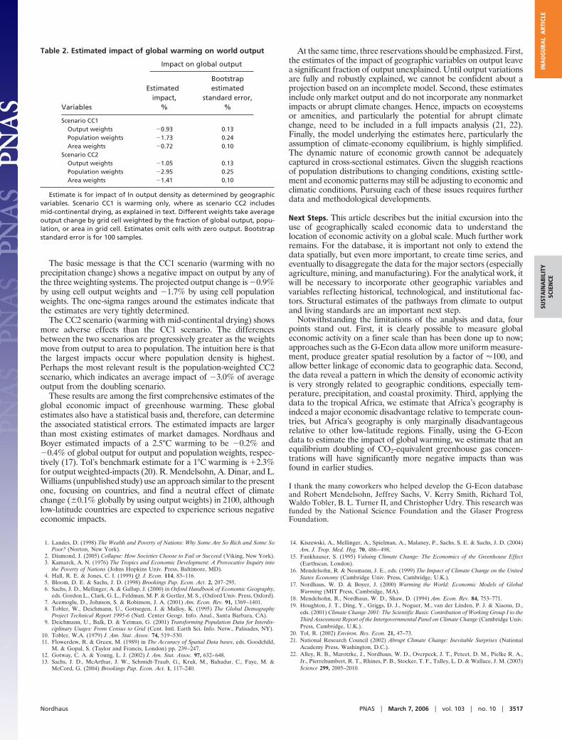
The basic message is that the CC1 scenario (warming with noprecipitation change) shows a negative impact on output by any ofthe three weighting systems. The projected output change is �0.9%by using cell output weights and �1.7% by using cell populationweights. The one-sigma ranges around the estimates indicate thatthe estimates are very tightly determined.

The CC2 scenario (warming with mid-continental drying) showsmore adverse effects than the CC1 scenario. The differencesbetween the two scenarios are progressively greater as the weightsmove from output to area to population. The intuition here is thatthe largest impacts occur where population density is highest.Perhaps the most relevant result is the population-weighted CC2scenario, which indicates an average impact of �3.0% of averageoutput from the doubling scenario.

These results are among the first comprehensive estimates of theglobal economic impact of greenhouse warming. These globalestimates also have a statistical basis and, therefore, can determinethe associated statistical errors. The estimated impacts are largerthan most existing estimates of market damages. Nordhaus andBoyer estimated impacts of a 2.5°C warming to be �0.2% and�0.4% of global output for output and population weights, respec-tively (17). Tol’s benchmark estimate for a 1°C warming is 2.3%for output weighted-impacts (20). R. Mendelsohn, A. Dinar, and L.Williams (unpublished study) use an approach similar to the presentone, focusing on countries, and find a neutral effect of climatechange (�0.1% globally by using output weights) in 2100, althoughlow-latitude countries are expected to experience serious negativeeconomic impacts.

At the same time, three reservations should be emphasized. First,the estimates of the impact of geographic variables on output leavea significant fraction of output unexplained. Until output variationsare fully and robustly explained, we cannot be confident about aprojection based on an incomplete model. Second, these estimatesinclude only market output and do not incorporate any nonmarketimpacts or abrupt climate changes. Hence, impacts on ecosystemsor amenities, and particularly the potential for abrupt climatechange, need to be included in a full impacts analysis (21, 22).Finally, the model underlying the estimates here, particularly theassumption of climate-economy equilibrium, is highly simplified.The dynamic nature of economic growth cannot be adequatelycaptured in cross-sectional estimates. Given the sluggish reactionsof population distributions to changing conditions, existing settle-ment and economic patterns may still be adjusting to economic andclimatic conditions. Pursuing each of these issues requires furtherdata and methodological developments.

Next Steps. This article describes but the initial excursion into theuse of geographically scaled economic data to understand thelocation of economic activity on a global scale. Much further workremains. For the database, it is important not only to extend thedata spatially, but even more important, to create time series, andeventually to disaggregate the data for the major sectors (especiallyagriculture, mining, and manufacturing). For the analytical work, itwill be necessary to incorporate other geographic variables andvariables reflecting historical, technological, and institutional fac-tors. Structural estimates of the pathways from climate to outputand living standards are an important next step.

Notwithstanding the limitations of the analysis and data, fourpoints stand out. First, it is clearly possible to measure globaleconomic activity on a finer scale than has been done up to now;approaches such as the G-Econ data allow more uniform measure-ment, produce greater spatial resolution by a factor of �100, andallow better linkage of economic data to geographic data. Second,the data reveal a pattern in which the density of economic activityis very strongly related to geographic conditions, especially tem-perature, precipitation, and coastal proximity. Third, applying thedata to the tropical Africa, we estimate that Africa’s geography isindeed a major economic disadvantage relative to temperate coun-tries, but Africa’s geography is only marginally disadvantageousrelative to other low-latitude regions. Finally, using the G-Econdata to estimate the impact of global warming, we estimate that anequilibrium doubling of CO2-equivalent greenhouse gas concen-trations will have significantly more negative impacts than wasfound in earlier studies.

I thank the many coworkers who helped develop the G-Econ databaseand Robert Mendelsohn, Jeffrey Sachs, V. Kerry Smith, Richard Tol,Waldo Tobler, B. L. Turner II, and Christopher Udry. This research wasfunded by the National Science Foundation and the Glaser ProgressFoundation.

1. Landes, D. (1998) The Wealth and Poverty of Nations: Why Some Are So Rich and Some SoPoor? (Norton, New York).

2. Diamond, J. (2005) Collapse: How Societies Choose to Fail or Succeed (Viking, New York).3. Kamarck, A. N. (1976) The Tropics and Economic Development: A Provocative Inquiry into

the Poverty of Nations (Johns Hopkins Univ. Press, Baltimore, MD).4. Hall, R. E. & Jones, C. I. (1999) Q. J. Econ. 114, 83–116.5. Bloom, D. E. & Sachs, J. D. (1998) Brookings Pap. Econ. Act. 2, 207–295.6. Sachs, J. D., Mellinger, A. & Gallup, J. (2000) in Oxford Handbook of Economic Geography,

eds. Gordon L., Clark, G. L., Feldman, M. P. & Gertler, M. S., (Oxford Univ. Press, Oxford).7. Acemoglu, D., Johnson, S. & Robinson, J. A. (2001) Am. Econ. Rev. 91, 1369–1401.8. Tobler, W., Deichmann, U., Gottsegen, J. & Malloy, K. (1995) The Global Demography

Project Technical Report 1995-6 (Natl. Center Geogr. Info. Anal., Santa Barbara, CA).9. Deichmann, U., Balk, D. & Yetman, G. (2001) Transforming Population Data for Interdis-

ciplinary Usages: From Census to Grid (Cent. Intl. Earth Sci. Info. Netw., Palisades, NY).10. Tobler, W.A. (1979) J. Am. Stat. Assoc. 74, 519–530.11. Flowerdew, R. & Green, M. (1989) in The Accuracy of Spatial Data bases, eds. Goodchild,

M. & Gopal, S. (Taylor and Francis, London) pp. 239–247.12. Gotway, C. A. & Young, L. J. (2002) J. Am. Stat. Assoc. 97, 632–648.13. Sachs, J. D., McArthur, J. W., Schmidt-Traub, G., Kruk, M., Bahadur, C., Faye, M. &

McCord, G. (2004) Brookings Pap. Econ. Act. 1, 117–240.

14. Kiszewski, A., Mellinger, A., Spielman, A., Malaney, P., Sachs, S. E. & Sachs, J. D. (2004)Am. J. Trop. Med. Hyg. 70, 486–498.

15. Fankhauser, S. (1995) Valuing Climate Change: The Economics of the Greenhouse Effect(Earthscan, London).

16. Mendelsohn, R. & Neumann, J. E., eds. (1999) The Impact of Climate Change on the UnitedStates Economy (Cambridge Univ. Press, Cambridge, U.K.).

17. Nordhaus, W. D. & Boyer, J. (2000) Warming the World: Economic Models of GlobalWarming (MIT Press, Cambridge, MA).

18. Mendelsohn, R., Nordhaus, W. D., Shaw, D. (1994) Am. Econ. Rev. 84, 753–771.19. Houghton, J. T., Ding, Y., Griggs, D. J., Noguer, M., van der Linden, P. J. & Xiaosu, D.,

eds. (2001) Climate Change 2001: The Scientific Basis: Contribution of Working Group I to theThird Assessment Report of the Intergovernmental Panel on Climate Change (Cambridge Univ.Press, Cambridge, U.K.).

20. Tol, R. (2002) Environ. Res. Econ. 21, 47–73.21. National Research Council (2002) Abrupt Climate Change: Inevitable Surprises (National

Academy Press, Washington, D.C.).22. Alley, R. B., Marotzke, J., Nordhaus, W. D., Overpeck, J. T., Peteet, D. M., Pielke R. A.,

Jr., Pierrehumbert, R. T., Rhines, P. B., Stocker, T. F., Talley, L. D. & Wallace, J. M. (2003)Science 299, 2005–2010.

Table 2. Estimated impact of global warming on world output

Variables

Impact on global output

Estimatedimpact,

%

Bootstrapestimated

standard error,%

Scenario CC1Output weights �0.93 0.13Population weights �1.73 0.24Area weights �0.72 0.10

Scenario CC2Output weights �1.05 0.13Population weights �2.95 0.25Area weights �1.41 0.10

Estimate is for impact of ln output density as determined by geographicvariables. Scenario CC1 is warming only, where as scenario CC2 includesmid-continental drying, as explained in text. Different weights take averageoutput change by grid cell weighted by the fraction of global output, popu-lation, or area in grid cell. Estimates omit cells with zero output. Bootstrapstandard error is for 100 samples.

Nordhaus PNAS � March 7, 2006 � vol. 103 � no. 10 � 3517

SUST

AIN

ABI

LITY

SCIE

NCE

INA

UG

URA

LA

RTIC

LE