Geographic Information System-Enabled Renewable …€¦ · GIS‐Enabled Renewable Energy Analysis Capability Project Final Report is the final ... Example of solar map ... based

Edmund G. Brown, Jr. Governor

GEOGR

PROJECT FINAL REPORT

PIER

alifornia Energy Commission Public Interest Energy Research Program

Thomas Baginski Lawrence Livermore National Laboratory

August 2011 CEC-500-2011-026

APHIC INFORMATION SYSTEM-ENABLED

RENEWABLE ENERGYANALYSIS CAPABILITY

FIN

AL P

ROJE

CT R

EPOR

T

Prepared For: C

Prepared By:

y roject Manager: Thomas Baginski

Author: Thomas Baginski Livermore, California 94550 Commission Contract No. 500-06-017

Prepared For:h (PIER)

gy Commission

Dianna Mircheva rs

Linda Spiegel

n Research Office

Laurie ten Hope H AND DEVELOPMENT DIVISION

obert P. Oglesby xecutive Director

Prepared By: Lawrence Livermore National LaboratorP

Public Interest Energy ResearcCalifornia Ener

Mike Kane and Contract Manage Office Manager Energy Generatio

Deputy Director ENERGY RESEARC

RE

DISCLAIMER

This report was prepared as the result of work sponsored by the California Energy Commission. It does not necessarily represent the views of the Energy Commission, its employees or the State of California. The Energy Commission, the State of California, its employees, contractors and subcontractors make no warrant, express or implied, and assume no legal liability for the information in this report; nor does any party represent that the uses of this information will not infringe upon privately owned rights. This report has not been approved or disapproved by the California Energy Commission nor has the California Energy Commission passed upon the accuracy or adequacy of the information in this report.

This document was prepared as an account of work sponsored by an agency of the United r Lawrence Livermore National

Security, LLC, nor any of their employees makes any warranty, expressed or implied, or assumes any legal liability or responsibility for the accuracy, completeness, or usefulness of any information, apparatus, product, or process disclosed, or represents that its use would not infringe privately owned rights. Reference herein to any specific commercial product, process, or service by trade name, trademark, manufacturer, or otherwise does not necessarily constitute or imply its endorsement, recommendation, or favoring by the United States government or Lawrence Livermore National Security, LLC. The views and opinions of authors expressed herein do not necessarily state or reflect those of the United States government or Lawrence Livermore National Security, LLC, and shall not be used for advertising or product endorsement purposes.

This work performed under the auspices of the U.S. Department of Energy by Lawrence Livermore National Laboratory under Contract DE-AC52-07NA27344.

LLNL-TR-422987

States government. Neither the United States government no

Preface

i

The California Energy Commission’s Public Interest Energy Research (PIER) Program supports public interest energy research and development that will help improve the quality of life in California by bringing environmentally safe, affordable, and reliable energy services and products to the marketplace. 

The PIER Program conducts public interest research, development, and demonstration (RD&D) projects to benefit California. 

The PIER Program strives to conduct the most promising public interest energy research by partnering with RD&D entities, including individuals, businesses, utilities, and public or private research institutions. 

PIER funding efforts are focused on the following RD&D program areas: 

• Buildings End‐Use Energy Efficiency 

• Energy Innovations Small Grants 

• Energy‐Related Environmental Research 

• Energy Systems Integration 

• Environmentally Preferred Advanced Generation 

• Industrial/Agricultural/Water End‐Use Energy Efficiency 

• Renewable Energy Technologies 

• Transportation 

GIS‐Enabled Renewable Energy Analysis Capability Project Final Report is the final report for the GIS Enabled Renewable Energy Analysis Capability project (Contract Number 500‐06‐017) conducted by Lawrence Livermore National Laboratory. The information from this project contributes to PIER’s Renewable Energy Technologies and Environmentally Preferred Advanced Generation Programs. 

For more information about the PIER Program, please visit the Energy Commission’s website at www.energy.ca.gov/research/ or contact the Energy Commission at 916‐327‐1551. 

Please cite this report as follows: 

Baginski, T.  2011.  GIS‐Enabled Renewable Energy Analysis Capability Project Final Report.  California Energy Commission, PIER Program.  CEC‐500‐2011‐026. 

ii

iii

Table of Contents

1.1.  Background and Overview ....................................................................................................... 3 

2.0  Project Approach ............................................................................................................................ 5 

.......... 5 

2.2.  Portal Management .................................................................................................................... 5 

2.3.  Interactive Web‐Based Mapping .............................................................................................. 5 

2.4.  GIS Support for the CHP Transmission Impact Analysis .................................................... 6 

3.0  Project Outcomes............................................................................................................................ 7 

3.1.  Preliminary Tasks, Task 1 ......................................................................................................... 7 

3.2.  Manage Portal, Task 2.1 ............................................................................................................ 7 

3.3.  Develop Renewable Energy Geospatial Data, Task 2.2 ........................................................ 8 

3.4.  Enhanced Renewable Energy Analysis Capability, Task 2.3 ............................................. 10 

3.5.  Outreach and Public Workshop, Task 2.4 ............................................................................ 15 

3.6.  CHP Analysis and Web Interface, Task 2.5 .......................................................................... 15 

3.7.  Economic Analysis and Web Interface, Task 2.6 ................................................................. 19 

3.8.  Reporting, Task 3 ..................................................................................................................... 21 

4.0  Conclusions and Recommendations ......................................................................................... 23 

5.0  References ..................................................................................................................................... 25 

Attachment I ............................................................................................................................................. 27 

Abstract ....................................................................................................................................................... v 

Executive Summary ................................................................................................................................... 1 

1.0  Introduction .................................................................................................................................... 3 

1.2.  Project Goals ............................................................................................................................... 3 

2.1.  Spatial Data .......................................................................................................................

iv

Table of Figures

....... 18 

ors, unless otherwise noted. 

Figure 1. Project website front page ...................................................................................................... 11

Figure 2. Example wind graphs ............................................................................................................. 12

Figure 3. Example of solar map viewer ................................................................................................ 13 

Figure 4. Example solar diurnal profile chart ...................................................................................... 13

Figure 5. Example map, Existing CHP capacity by city ..............................................................

Figure 6. Example of the CHP map viewer .......................................................................................... 19

Note: All tables, figures, and photos in this report were produced by the auth

v

Abstract

This report summarizes the work completed by Lawrence Livermore National Laboratory and BEW Engineering under Contracts 500‐06‐017 and 500‐06‐017 Amendment #1. The report gives a project background, lists the project goals, and summarizes the project outcomes by task. The report highlights enhancements made to the project website, the California Renewable Resource Portal, available at https://calrenewableresource.llnl.gov/. The California Renewable Resource Portal consolidates and presents a large amount geographically‐characterized wind, solar, geothermal, biomass, small hydropower and combined heat and power data and related information in an easy to use graphical format. By simplifying access to existing California renewable datasets, the website will help avoid costly duplication of effort, thereby benefitting California ratepayers and making it easier to implement California renewable energy and combined heat and power policy goals. The report attachment summarizes the Combined Heat and Power Transmission Impact Analysis completed by BEW Engineering.  

Keywords: Combined heat and power, CHP, Renewables, wind, solar, geothermal, biomass, hydropower, GIS, geographic information system, California Renewable Resource Portal

vi

1

tal pping, and geographic information system support for the 

the project replaced the commercial map server previously used in a pilot project  client.  The project simplified the mapping interface to 

 to 

 derive approximate es with 

 fined in the project scope of work. The project completed all 

roject  tasks and delivered all major products as  specified  in  the  scope of work.   Where  the eliverable  varied  from  those  originally  listed  in  the  scope  of  work,  explanations  and 

justifications are given.  The report lists all the geospatial data used or developed for the project   support  analysis  of  renewable  resource  and  combined  heat  and  power.    The  report  also eviews the enhancement and additions made to the project website.  Some highlights include: expanding  the wind  interactive mapping  application  to  cover  all  five major wind  resource reas, adding Web  sections  for  solar, geothermal, biomass,  small hydropower, and combined heat and power, and adding interactive map viewers for solar, geothermal, and combined heat nd power. 

Executive Summary

This project developed tools that incorporate Web and geographic information system technologies that provide forecasting and planning information to support analysis of renewable generation and conventionally fueled combined heat and power.  Through this project, the research team developed an interactive Web‐based capability that presents text, charts, and maps that help plan renewable and combined heat and power sites. 

Lawrence Livermore National Laboratoryʹs approach focused on four items: spatial data, pormanagement, interactive Web maCombined Heat and Power Transmission Impact Analysis.  For spatial data, the project focusedon regions with existing developed resource capacity, and on regions previously identified as having known, but underdeveloped resource potential.  The project first evaluated the availability and coverage of existing data sources to avoid duplication of past efforts.  For cases where existing data sources were unavailable or insufficient, the project developed new or updated geospatial data from source data.  For portal management, the project enhancements were incorporated into the California Renewable Resource Portal available at https://calrenewableresource.llnl.gov/.  The website follows modern Cascading Style Sheets‐based styling and Web page authoring to create a user‐friendly website layout and navigation.  It also includes explanatory text and references where appropriate.  For the interactive maps on the website, with an open‐source map server andimprove usability and performance.  For the transmission impact analysis, the project neededassociate existing and potential combined heat and power sites with their connections point with the transmission grid.  The project used available information tolocations for facilities. Based on the identified location, the project associated the facilititheir transmission grid connection point. 

The project outcomes section reviews  the project by  task, and summarizes each  task outcomeand corresponding products as depd

tor

a

a

2

sis completed by BEW Engineering is documented in an  analysis studied the transmission benefits of increasing the 

rces onto the California transmission grid. 

 2010.  It provides a ranked list of regions where 2010 combined heat and power development will 

 ers evaluate critical resource and siting issues in the areas of wind, 

es.  te  t 

accurate, geospatial 

d 

The transmission impact analyattachment to this report.  Thepenetration of combined heat and power resouDepending on where the new combined heat and power potential is developed, the new capacity can improve or worsen transmission congestion problems on the grid. The analysis provides a way to optimize combined heat and power development in strategic areas that have technical potential and reduce transmission congestion.  The analysis evaluates existing combined heat and power resources and potential combined heat and power resources in

improve transmission reliability. 

The project resulted in a publicly available website that presents geospatial data and other information for renewable and combined heat and power resources.  The website will help thedecision makers and developgeothermal, biomass, solar, small hydropower, and combined heat and power.  The website consolidates and presents a large amount of resource information, statistical study data, land use, and demographic planning data in a manner that is readily accessible to interested partiDuring the project period, the website provided the ability to integrate, access, and disseminaspatial data for California analysis needs as it came available.  The combined heat and powertransmission impact analysis examined key resource development concerns for combined heaand power. 

The project benefited California by: 

• Evaluating and developing implementation paths for achieving renewable resource goals beyond 2010 including 33 percent renewables by 2020. 

• Tracking development and repowering with a database of information useful for resource assessments and siting. 

• Providing consistent and updated information on renewable resources for research angeneral public awareness. 

1.0 Introduction

3

‐06‐017 and 500‐06‐st contract was signed in December 2006.  Amendment  #1 was 

 Laboratory (LLNL) is the lead contractor.  A portion  sub‐contracted to BEW Engineering (BEW).  Work started nded contract ended January 29, 2010. 

This er the contract. The report lists the project goals.  It ect approach.  Next, it reviews the project outcomes for each task in 

the udes with recommendations and the benefits to California. 

1.The  and geographic information system  planning information benefitting an energy generation and conventionally fueled combined n interactive Web‐based capability 

 analysis of renewable and CHP arlier Energy Commission‐supported project at LLNL developed a 

de dated wind data and provided the capability to display data , siting, and repowering needs.  The current project effort enhanced orm into a Web‐based renewable portal that contained resource  resource areas (wind, solar, geothermal, biomass, and 

tial. 

The project objectives stated in the contract include the following: 

• Provide an interactive, analytical decision tool to evaluate critical resource and siting issues in the areas of wind, geothermal, biomass, solar, small hydropower, and combined heat and power. 

• Consolidate resource information, statistical study data, land use, and demographic planning data to track and forecast development trends and to perform tradeoffs on development options. 

• Provide and maintain the ability to integrate, access, and disseminate new spatial data for California analysis needs and work with the existing state GIS infrastructure to archive valuable resource information. 

• Provide analysis on key resource development concerns including combined heat and power, wind repowering, solar photovoltaic (PV) development, concentrated solar power resource profiles, transmission corridors, environmental impact areas, distribution issues, and tracking of land use/right‐of‐way issues. 

1.1. Background and Overview The California Energy Commission funded this project under Contracts 500017 Amendment #1.  The firsigned in May 2007.  Lawrence Livermore National

 of a task added in Amendment #1 is on the project in February 2007.  The ame

 report summarizes work completed undthen summarizes the proj scope of work.  Finally, it concl

2. Project Goals  purpose of this project is to develop tools that incorporate Web (GIS) technologies that provide forecasting and market with an increasing mix of renewable  heat and power (CHP).  Through this project, a

 text, charts, and maps that aidwas developed that presentssiting and planning.  An e

monstration platform that consoli for wind resource planning

 the demonstration platf information for all renewable

small hydropower) and for combined heat and power poten

4

.2.1. List of Project Tasks fied in the scope of work: preliminary activities, technical al tasks contain most of the project work that focused on 

ls.  The individual subtasks are listed below. 

3.3  Final meeting 

1The project has three main parts identitasks, and reporting tasks.  The technicthe meeting the project goa

• 1 Preliminary tasks 

o 1.1 Attend kick‐off meeting 

o 1.2  Describe synergistic projects 

o 1.3  Identify required permits 

• 2 Technical tasks 

o 2.1  Manage portal 

o 2.2  Collect and develop renewable energy geospatial data 

o 2.3  Enhanced renewable energy analysis capability 

o 2.4  Outreach and public workshop 

o 2.5  CHP analysis and Web interface 

o 2.6  Economic analysis and Web interface 

• 3 Reporting tasks 

o 3.1  Progress reports 

o 3.2  Final report 

o

5

 and 

a 

  Altamont, 

 attribute data.  For all developed or updated data sets, the project team produced standardized metadata that documented the data, source, 

ts were  not 

mmission contract managers on making 

omes 

ebsite follows modern CSS‐based styling and Web 

 ity. 

 Google Maps. 

2.0 Project Approach

2.1. Spatial Data One of the major project goals was to gather or generate geospatial data layers appropriate to support renewable and CHP resource analysis.  The project used the following approach to meet this goal.  Data layer development efforts focused on regions surrounding existingpotential resource areas within California.  The project first evaluated the availability and coverage of existing data sources to avoid duplication of past effort.  In many cases existing datsets met the project needs.  For cases where existing data sources were not available or insufficient, the project developed new or updated geospatial data from source data.  Forexample, the project created a new parcel based wind project area data set for theSolano, and San Gorgonio wind resource areas.  The project team used published environmental impact reports and other planning documents available from state and county sources to identify parcels with existing and planned wind projects.  The team then digitized the identified parcels and attached appropriate

attributes, and other useful information.  All original and updated geospatial data sedelivered to the Energy Commission contract managers on a data disk.  The project didmake the data available to the public on a statewide clearing‐house as intended at the start of the project.  The project team deferred to the Energy Cothe data available if they decide it is appropriate and there are no security constraints. 

The specific data sets gathered and developed are documented below in the Project Outcsection. 

2.2. Portal Management The project was tasked with enhancing the usability, maintainability, and performance needed to serve the renewable data and analysis capability of a Web‐based portal.  The project enhancements were incorporated into the California Renewable Resource Portal available at https://calrenewableresource.llnl.gov/.  The wpage authoring to create a user‐friendly website layout and navigation.  It also includes explanatory text and references where appropriate.  To minimize system administration expenses, the project team moved the website from its own stand‐alone Web server to an institutionally supported common Web server at LLNL.  The institutionally supported Webserver also provides performance improvements and fail‐over support that improve reliabil

2.3. Interactive Web-Based Mapping The project website includes several interactive Web mapping pages.  The project replaced the commercial map server used in a pilot project with an open‐source map server and client.  Theproject simplified the mapping interface to improve usability and performance.   The projectalso replaced internally generated base layers with base layers provided by

6

he Web‐mapping tool developed at LLNL for the Altamont wind resource area through the  proprietary commercial software that need to run on its software required an initial purchase fee and an annual 

re 

hat was available when it was developed, but newer Web mapping technology is now available without some of the previous disadvantages. 

improvements using open source Web mapping  

The 

mple to use, free, and he final Web mapping tools were deployed using pre‐ is needed at run time.  This improves performance 

e project needed to associate existing and potential CHP sites with their  then 

isting CHP site tabular data contained county and city information.  The project located the facility at the centroid of the reported city.  The CHP potential sites for large 

 ed the lengthy task of looking up the exact location of ta. 

ies with their transmission grid ses 

 the point locations of facilities with their closest bus point  facility 

st, the bus associations for a few large facilities were manually checked based on the name, load, and generation fields in the bus data set.  A small number of these large facilities were manually reassigned to more appropriate collocated or nearby busses.   

Tearlier pilot project was developed withown mapping server.  The map server maintenance fee for updates and support.  The client interface and the server product weclosely coupled and could not be changed independently.  This pilot project implementation was appropriate for the technology t

The project implemented the Web mapping products.  The Web client uses the OpenLayers framework (http://www.openlayers.org).  Theinterface implemented is similar to common Web mapping service such as Google Maps.  Web client can also support several data formats from multiple sources using open Web mapping standards.  The Web mapping server was developed using MapServer (http://mapserver.org/) and TileCache (http://tilecache.org/).  Both are sisupport open Web mapping standards.  Tgenerated map tiles so that no map serverand simplifies server maintenance. 

2.4. GIS Support for the CHP Transmission Impact Analysis For Task 2.5 thconnection points with the transmission grid.  The location process is discussed first, andthe transmission grid association is discussed second. 

The exact location of the existing and potential CHP sites was not directly available in the source data.  The project used available information to derive approximate locations for facilities.  The ex

industrial facilities contained ZIP‐code information.  The project team made some updates tothe ZIP‐code data to remove some outdated values and replace them with current values.  The facility location was then assigned based on the centroid of the ZIP‐code.  This location processwas sufficient for the analysis and avoidthe hundreds of facilities in the source da

Based on the identified location, the project associated the facilitconnection point.  Facilities can connect to the transmission network at node called a bus.  Buare generally located at substations.  More than one bus can be collocated at the same substation.  LLNL staff matchedlocation using GIS.  The team then confirmed that the reported electric utility of thematched the electric utility of the closest bus.  For cases of mismatch, the closest bus from the same electric utility was found.  La

7

ve in Section 1.2.1.  This section reviews the outcome and  

0, 2008.  Letters the February 2007 progress 

uired was submitted at the February 2007 

eted by 

the 

e project released the remaining task deliverables.  The usage and user feedback repository is accessible by Energy Commission contract managers and project staff.  This section 

 guide is available on the website and is 

ust 2009. 

3.0 Project Outcomes The project tasks are listed abodeliverables for each task.  The project task number is listed in each heading since it differs fromthis documents section numbering. 

3.1. Preliminary Tasks, Task 1 All three preliminary task have been completed.  The initial kickoff meeting for 1.1 was held February 1, 2007.  The kickoff meeting for the CHP task was held March 2describing the synergistic projects for 1.2 were submitted with report.  A letter for 1.3 stating no permits were reqkickoff meeting and included with the February 2007 progress report. 

3.2. Manage Portal, Task 2.1 The goal of this task is to enhance the usability, maintainability, and performance needed to serve the renewable data and analysis capability.  It was an ongoing task that scheduled from project start to November 2009.  All management activities for this task were complJanuary 2010. 

In 2007 the project team investigated a Web usage reporting system, performed system administration, and created an internal development server instance. 

In 2008 the project website was migrated to the institutional Web server as discussed in section 2.2.  During this time the research team also removed the pilot project Web map interface for Altamont Pass. 

In 2009, th

of the website is password‐restricted.  The userimplemented as an annotated site map. 

3.2.1. Task Deliverables Summary The task deliverables and completion date or statuses are: 

• Web‐enabled Renewable Portal.  This was released starting in December 2008 and is final as of January 2010. 

• Usage and User Feedback Repository.  This was delivered in Aug

• User Guide Report.  Implemented as an annotated site map available on the website.  It is final as of January 2010. 

8

 the 

 was delivered to the Energy Commission contract managers.  For data sets that LLNL did not 

data used for e included in this list. 

  can be accessed at http://rredc.nrel.gov/solar/old_data/nsrdb/1961‐1990/  

This data set contains solar radiation information for 105 locations within California.  It contains or all locations using interpolation when necessary.  The 

l  

NL extracted  that were used extensively in the solar section of the project 

S  in 

et contains the a 200 m grid data with: 1) wind speed and wind power at 30 m, 

 the wind section of the project website. 

3.3. Develop Renewable Energy Geospatial Data, Task 2.2 LLNL staff compiled and generated geospatial data layers appropriate to support renewable resource analysis and address renewable development challenges.  This section describesdata used during the project. 

For data sets that LLNL generated, updated, or significantly modified, a copy of the new data

originate, a description of the data and a reference to the definitive source are included.   In some cases, due to copyright or security restrictions, LLNL cannot redistribute this project.  Descriptions of these restricted data ar

3.3.1. Geospatial Data Layers for Renewable Energy National Solar Radiation Database 1961-1990 This data set contains solar radiation information for 10 monitoring station locations within California for 1961‐1990.  The data contain hourly time series when available.  Some 40 km gridded data are available that were interpolated from the point locations.  LLNL did not directly use this data.  However, it does provide a historical time series of data if needed.  Thedatabase

National Solar Radiation Database 1991-2005 Update

complete hourly data from 1991‐2005 fupdate also has 10 km gridded data available for 1998‐2005 which are the output of a modebased on satellite data.   The gridded data contain hourly solar radiation estimates for the entireeight‐year time period.  Approximately 4200 data points fall within California.  The original data can be accessed at http://rredc.nrel.gov/solar/old_data/nsrdb/1991‐2005/.   LLsubsets of these data for Californiawebsite.   

California Wind Energy Resource Maps This data set was produced by AWS Truewind for the California Energy Commission (AWTruewind  2006).  It was originally published in 2002 and updated for some resource areas2006.  The data s50 m, 70 m, and 100 m; 2) Weibull distribution parameters C and k at 50 m.  The data set also contains a 2 km grid data with wind rose frequencies, mean speeds, and percentage of energy.  LLNL used these data extensively in

Turbine and Turbine Footprints for Major Wind Resource Areas These data were originally produced at LLNL in 2003 and 2004 as part of the pilot project.   The footprint data are available for the Altamont, Pacheco, San Gorgonio, Solano, and Tehachapi wind resource areas.  The individual turbine location data and footprint data were not updated for this project.  These data are shown in the Wind section of the project website.    

9

 set using current aerial photography, parcel 

w orated into this data set and not listed separately. 

n Geothermal Resource Areas l 

res reported in the Strategic d Tiangco 2005) and the Intermittency Analysis 

007).  This data set is used in the geothermal section of the project website.     

 shapefile named: shp.   

LLNL used the 72 Hydro‐Climate Data e of the project website.  The 

 from the U.S. Geological Survey water data website at gs.gov/nwis/. 

capacity by county for 2005.  It   

mmission contract managers as a dBase table named 

y for 2007.  It is based on data in An Assessment of Biomass Resources in California, 2007 by the California Biomass 

ebsite. 

LLNL created an updated wind project area dataoutlines, and available planning documents to incorporate any newly developed areas for the Altamont, San Gorgonio, and Solano WRAs.   LLNL also included planned wind energy development projects into this data set based on sites reported in available environmental impact report (EIR) data.  EIR data was listed as a separate item in the ʺList of Existing and NeData Layersʺ deliverable.  It was incorp

The data were delivered to the Energy Commission contract managers as shapefiles named: wind_ca_footprint.shp, wind_ca_turbines.shp, and wind_ca_project_area.shp. 

California KnowThese data display California known geothermal resources areas and their current and potentiageneration capacity.  The data set was received from the California Spatial Information Library.  LLNL then updated the spatial and attribute data to reflect the figuValue Assessment project (Sison‐Lebrilla anProject (Davis et al. 2LLNL did not use the California geothermal well locations data set listed in the original datalist. 

The data were delivered to the Energy Commission contract managers as ageo_resource_areas.

National Water Information System This data was developed by the U.S. Geological Survey and reports real time stream flow information for more than 400 sites within California.  Network sites within California on the stream flow data sites pagoriginal data are availablehttp://waterdata.us

Existing Biomass by County This tabular data set contains the existing and planned biomass is based on data in An Assessment of Biomass Resources in California, 2007 by the CaliforniaBiomass Collaborative (Williams 2008).  These data are used in the biomass section of theproject website. 

The data were delivered to the Energy CobiomassExistingByCounty2005.dbf 

Biomass Technical Potential by County This tabular data set contains the technical potential for biomass by count

Collaborative (Williams 2008).  These data are used in the biomass section of the project w

The data were delivered to the Energy Commission contract managers as a dBase table named biomassTechPotentialByCounty2007.dbf 

10

 agricultural data based on data in An Assessment of Biomass Resources in 08).  The Forest data were 

These data are used in the 

 as dBase tables named  

include: multi‐source land  lands.  These data were 

and standardized into  from the California  

Monitoring Program  used the 2006 version of 

ovides an inventory of all the protected open space  Spatial Information 

ta.  This was completed in September 2009. 

Land Area in Biomass-Related Cover Types These two tabular data sets contain the land area in forest and agricultural cover types summed by county.  TheCalifornia, 2007 by the California Biomass Collaborative (Williams 20calculated by LLNL based on FRAP land cover data (FRAP 2002).  biomass section of the project website. 

The data were delivered to the Energy Commission contract managersbiomassForestAreaByCounty.dbf, and biomassAgricultureAreaByCounty.dbf

Land Use Data The project team gathered several statewide land use data sets that cover, public and conservation lands, easement areas, state and federalall downloaded from the California Spatial Information Library at http://atlas.ca.gov/download.html?sl=casil 

General Plan Data All county general plans and many city general plans are integrated thirteen consistent land use classifications. This data set was downloadedSpatial Information Library at http://atlas.ca.gov/download.html?sl=casil.

Farmlands Data The California Department of Conservation Farmland Mapping and (FMMP) data identifies agricultural land resources by county.  LLNLthe data.  It can be accessed on the FMMP website at: http://www.conservation.ca.gov/dlrp/FMMP/Pages/Index.aspx.

Protected Areas The California Protected Areas Database prlands in the State.  This data set was downloaded from the CaliforniaLibrary.  The data are documented at: http://www.calands.org/ 

The airspace, Indian lands, and climatic data sets listed on the original data list were not gathered or used for this project. 

3.3.2. Task Deliverables Summary The task deliverables and delivery status are: 

• List of existing and new data layers.  This was completed in November 2007. 

• Data sets and metada

3.4. Enhanced Renewable Energy Analysis Capability, Task 2.3 The goal of this task is to develop a Web based analysis capability focusing on each of the renewable resource areas including wind, solar, geothermal, biomass, and small hydropower.  The task includes several subtask and deliverables which are described below.  The main 

11

e front page of the website is shown 

d at er at 50m (AWS Truewind  2006).  Where 

ind 

For four of the wind resource areas, LLNL developed wind profile graphs based on AWS Truewind modeled wind data (AWS Truewind  2006).  The graphs show average daily wind power by month, average daily wind speed by month, hourly variation of average wind speed by season, and average wind speed by height.  These were not included in the original task list.  Two example graphs are shown in Figure 2.  Both are for the same location in San Gorgonio.  

website of the project website is https://calrenewableresource.llnl.gov/.  All enhancements completed for this project can be access via the website.  Thin Figure 1. 

 Figure 1. Project website front page Source: Lawrence Livermore National Laboratory

3.4.1. Wind Website Enhancements The wind section enhancements are available on the website at https://calrenewableresource.llnl.gov/wind/.  The website now includes pages for the five majorwind resource areas in California: Altamont, Tehachapi, San Gorgonio, Solano, and Pacheco Pass.  The website also includes an interactive map viewer for these five wind resource areas.  The map viewers incorporate the latest AWS Truewind data including: annual wind spee30m, 50m, 70m, and 100m; and annual wind powavailable the map viewer includes existing and proposed wind development parcels.  The wsection also contains links to the Electronic Wind Performance Report Summary website as listed in the scope of work. 

12

month.  The right shows the 

olar/.  The solar section includes maps and tables of solar  animation of seasonal variation in current National Solar Radiation ion 3.3.1.  The solar section has a sonal solar radiation using a 10km 

monitoring station within California  page for a station has graphs of  relative frequency by season, and  links to the raw NSRDB data for ors create summary points at the  as is shown for the NSRDB source calculator application for a 

scope of work are met by this 

w.  Figure 3 shows an NSRDB station location near Livermore, CA.  Figure 4 shows the corresponding diurnal profile chart 

The left graph show modeled average daily wind power at 50m by hourly variation of average wind speed at 50m by season. 

Figure 2. Example wind graphs Source: Lawrence Livermore National Laboratory

3.4.2. Solar Website Enhancements The solar section enhancements are available on the website at https://calrenewableresource.llnl.gov/sresource potential by county, solar profiles by county and ansolar radiation.  The solar section make extensive use of the Database Update 1991‐2005 (NSRDB) as documented in Sectstatewide interactive map viewer that shows annual and seagrid.  The viewer also displays the location of all NSRDB and provides links to a detail page for the station.  The detailyear to year radiation, diurnal profile by season, cumulativedaily average by month.  The detail page also provides directthe station.  For counties without an NSRDB station, the authcounty seat and generated similar summary data and chartsstations.  The map viewer can link to the PVWATTS solar regiven location.  All the listed solar enhancements from the application and the accompanying Web pages.  

Examples of the solar map viewer and charts are shown belo

that is included on the station detail page. 

 Figure 3. Example of solar map viewer Source: Lawrence Livermore National Laboratory

 Figure 4. Example solar diurnal profile chart Source: Lawrence Livermore National Laboratory

3.4.3. Geothermal Website Enhancements e geother  website at 

13

ction contains a table of the existing zes 

geothermal capacity by county using maps and tables.  An interactive geothermal map viewer 

Th   mal section enhancements are available on thehttps://calrenewableresource.llnl.gov/geothermal/.  This seand predicted capacity at known geothermal resource areas.  The website section summari

14

lows the user to query  list facility specific data or 

d m 

e. 

ass 

ides links to real‐time flow data available through the USGS.  The section meets all the listed hydropower enhancements from the scope 

ource predictions from environmental models se other enhancement was given a 

Study  

completed this task in collaboration with the U.C. Berkeley Fire Center.   A copy of the report ruary 2008.  The feasibility 

 for 

ewable Portal.  This was completed in 

Wind Section Enhancements.  This was completed in August 2009. 

displays the footprints of known geothermal resource areas and alexisting and potential capacity for these areas.  The website does notgive the exact location of any existing individual geothermal facilities.  All data are aggregateto the level of known geothermal resource areas.  All the listed geothermal enhancements frothe scope of work are met by the geothermal section of the websit

3.4.4. Biomass Website Enhancements The biomass section enhancements are available at https://calrenewableresource.llnl.gov/biomass/.  This section has static maps and tables of biomass potential by county.  It also has maps and tables of the total area in potential biomrelated land use categories summarized by county.  It also includes links to the Energy Commission funded California Biomass Collaborative website.  The section meets all the listed biomass enhancements from the scope of work. 

3.4.5. Hydropower and Water Resource Website Enhancements The hydropower and water resource section enhancements are available at https://calrenewableresource.llnl.gov/hydro/.  The section summarizes hydropower by countyusing maps and tables.  It provides a visualization of the variation in runoff during droughtyears and wet years.  It shows the location and prov

of work except for the listing of hydro resrelevant to RPS.  This enhancement was not included becauhigher priority. 

3.4.6. FeasibilityThe feasibility study of future website enhancements was completed in 2007.  The project team

was submitted to the Energy Commission contract manager in Febstudy addressed the potential tasks described in the contract, and it proposed cost estimateseach task. 

3.4.7. Task Deliverables Summary The task deliverables and completion date or statuses are: 

• List of Enhanced Analysis Capabilities for the RenFebruary 2009. 

• Critical Project Review Report.  The Energy Commission contract managers and project staff held a critical project review in August 2008.  The report was submitted at the review. 

•

• Solar Section.  This was completed in August 2009 

• Hydropower and water resource section.  This was completed in November 2009. 

• Geothermal Section.  This was completed in August 2009. 

• Biomass Section.  This was completed in November 2009. 

15

ts feasibility study.  This was delivered in February 2008 

 at alysis and/or renewable energy.  LLNL staff presented a talk 

ted for Renewable Energy Analysisʺ at the Consortium on Climate Energy 

ting in August 2007.  Copies of both presentation slides were delivered to the 

at ility 

t of 

is was completed in December of 2008. 

ansmission impact analysis was subcontracted 

n a r in 

ated, updated, or significantly modified a copy of the new data 

• Future website enhancemen

3.5. Outreach and Public Workshop, Task 2.4 The goal of this task is to promote the capabilities of the project and website to interested stakeholders.  The task specifies that the project shall staff present appropriate informationtwo conferences related to GIS antitled “Developing a Web‐GIS Tool for Renewable Resource Analysis in California” at the Association of American Geographers Annual Meeting in April 2007.  LLNL staff also presena talk titled ʺWeb Tools and Environment meethe Energy Commission contract manager.  The scope of work also specified presenting on project to interested stakeholders at a public workshop hosted by the Energy Commission.  LLNL and BEW Engineering presented a summary of CHP work to date in December 2008 the Commission hosted ʺWorkshop on Geographical Information System Enabled Capabfor Combined Heat and Power.ʺ  Copies of the presentation material were delivered to the Commission contract mangers after the workshop. 

3.5.1. Task Deliverables Summary The task deliverables and completion date or statuses are: 

• Copies of conference presentation materials.  This was completed in April and Augus2007. 

• Copies of workshop presentation materials.  Th

3.6. CHP Analysis and Web Interface, Task 2.5 The goal of this task is to compile or generate geospatial data layers appropriate to support analysis and siting of CHP and address development challenges.  An additional goal is to assessthe impact on electrical transmission grid congestion of adding potential CHP resources.  This task was added through Amendment #1.  The trto BEW Engineering (BEW). 

3.6.1. Geospatial Data Layers for CHP Analysis LLNL compiled and generated geospatial data layers appropriate to support CHP resource analysis and to conduct the CHP transmission impacts analysis.  The data layers are based olist of existing and new data layers submitted to the Energy Commission contract manageJune 2009.  This section describes the data used during the project. 

For data sets that LLNL generwas delivered to the Energy Commission contract managers.  For data sets that LLNL did not originate, a description of the data and a reference to the definitive source is included.   In some 

16

estricted data are included in this list. 

alifornia

 There are  database does not have the city and county fields to 

I “Industrial Sector Combined Heat and Power and Export HP sites in California (Darrow et 

The research team used the California electricity transmission bus location data set from the Strategic Value Analysis Project (Davis Power Consultants et al. 2005) and the Intermittency Analysis Project (Davis et al. 2007).  The research team updated this data set with load, generation, and name data from the PowerWorld software package that BEW is using for the transmission impact analysis.  Due to data use constraints, the authors cannot redistribute this.  The authors used the data for internal analysis. 

California Electricity Transmission Network and Flow BEW maintains a model of the California electrical transmission system using proprietary data and the PowerWorld software package.  BEW used data developed for previous projects including the Intermittency Analysis Project (Davis et al. 2007) and the Northern California Regional Integration of Renewables Project to model current and future electric demand, generation, and transmission flows.  As stated in the scope of work, the network and transmission data is proprietary and will stay with BEW. 

Natural Gas Service Areas LLNL constructed a natural gas service area data layer using the Energy Commission provided natural gas service areas data set. 

cases, due to copyright or security restrictions, LLNL cannot redistribute data used for this project.  Descriptions of these r

Existing CHP Sites in CThe authors used the ICF International (ICFI) “Combined Heat and Power Installation Database” as the basis for mapping existing CHP sites in California (Hampson 2009).  944 records in the current version of the California database.  Theaddress or exact location of the sites.  The research team used the approximate the site locations. 

The data were delivered to the Energy Commission contract managers as a shapefile named chp_2009_existing.shp. 

CHP Potential Sites The research team used the ICFMarket Potential” data set as the basis for mapping potential Cal. 2009).  This database is documented in the May 2009 report cited above.  ICFI provided LLNL with its draft results for the report.  The research team used the draft results in its analysis because they were what were available when the authors needed the data.  There are minor differences to the final report values.  There are 947 sites in our copy of the data set.  As with the existing site database, the address or exact location of the site is not reported.   The authors used the ZIP code, city, and county fields to approximate the site locations. 

The data were delivered to the Energy Commission contract managers as a shapefile named chp_mipd_final.shp.   

California Electricity Transmission Bus Locations

17

Commission contract managers as a shapefile named 

 provided natural gas pipeline data set.  LLNL  already has a copy of this data set 

 in Section 3.3.13.3. 

completed by BEW.  The work is documented in the LLNL provided spatial data input and mapping 

project websites at The features developed for the Web interface are  the Energy Commission contract manager in  are summarized by county and city using tables  of existing CHP resources is shown in Figure 5.  

 are summarized into a series of Web  report to display the results of the 

nalysis.  The website also includes an interactive Web map viewer for CHP resources.  The map view displays map layers of existing capacity by county, existing capacity by city, onsite CHP potential, export CHP potential, and the summer 2020 case from the Transmission Impact Analysis.  An example from the CHP map viewer is shown in Figure 6. 

The data were delivered to the Energy natural_gas_service_area.shp. 

Natural Gas Pipelines The research team used the Energy Commissiondid not make any modifications.  The Commission

The land use data sets are documented above

3.6.2. CHP Transmission Impact Analysis The CHP transmission impact analysis was attached report.  As discussed in Section 2.4, support for this analysis. 

3.6.3. CHP Web Interface The CHP Web interface is available on the https://calrenewableresource.llnl.gov/chp/.  based on a list of enhancements submitted toAugust 2009.  Existing and potential capacityand maps.  An example map from the websiteThe results of the transmission impact analysis report

 maps from thepages.  The pages use tables, charts, anda

 Figure 5. Example map, existing CHP capacity by city Source: Lawrence Livermore National Laboratory

18

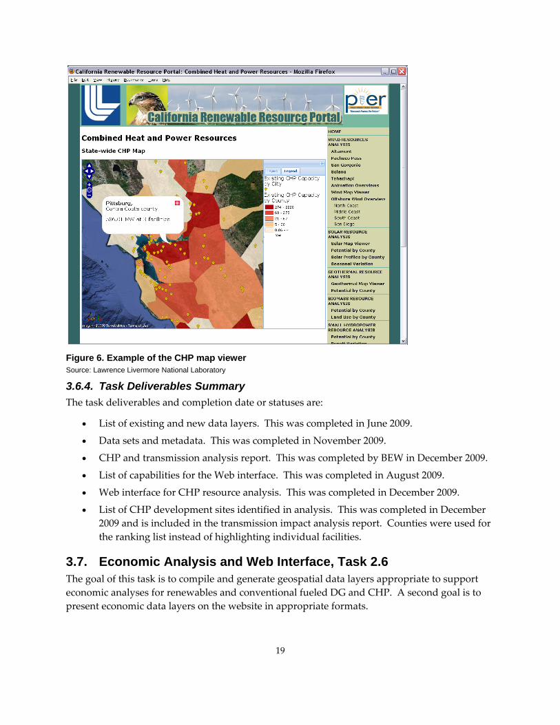
 Figure 6. Example of the CHP map viewer Source: Lawrence Livermore National Laboratory

3.6.4. Task Deliverables Summary

19

d new data layers.  This was completed in June 2009. 

ompleted in November 2009. 

Web interface for CHP resource analysis.  This was completed in December 2009. 

pport 

 formats. 

The task deliverables and completion date or statuses are: 

• List of existing an

• Data sets and metadata.  This was c

• CHP and transmission analysis report.  This was completed by BEW in December 2009. 

• List of capabilities for the Web interface.  This was completed in August 2009. 

•

• List of CHP development sites identified in analysis.  This was completed in December 2009 and is included in the transmission impact analysis report.  Counties were used for the ranking list instead of highlighting individual facilities. 

3.7. Economic Analysis and Web Interface, Task 2.6 The goal of this task is to compile and generate geospatial data layers appropriate to sueconomic analyses for renewables and conventional fueled DG and CHP.  A second goal is to present economic data layers on the website in appropriate

20

onomic Analysis  on a list of existing and new data 

is section 

Commercial and Industrial Electricity Rates s maintained on the Energy Commission Energy Almanac 

K field that matched the NAME field in the Energy Commission provided Electric Service Area 

 visualization and 

 managers as dBase tables named bf, econ_elec_rate_residential.dbf, 

and econ_gsp_deflator.dbf. 

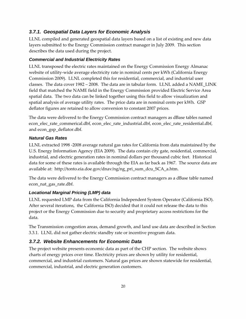
Natural Gas Rates LLNL extracted 1998 ‐2008 average natural gas rates for California from data maintained by the U.S. Energy Information Agency (EIA 2009).  The data contain city gate, residential, commercial, industrial, and electric generation rates in nominal dollars per thousand cubic feet.  Historical data for some of these rates is available through the EIA as far back as 1967.  The source data are available at:  http://tonto.eia.doe.gov/dnav/ng/ng_pri_sum_dcu_SCA_a.htm. 

The data were delivered to the Energy Commission contract managers as a dBase table named econ_nat_gas_rate.dbf. 

Locational Marginal Pricing (LMP) data LLNL requested LMP data from the California Independent System Operator (California ISO).  After several iterations,  the California ISO) decided that it could not release the data to this project or the Energy Commission due to security and proprietary access restrictions for the data. 

The Transmission congestion areas, demand growth, and land use data are described in Section 3.3.1.  LLNL did not gather electric standby rate or incentive program data. 

3.7.2. Website Enhancements for Economic Data The project website presents economic data as part of the CHP section.  The website shows charts of energy prices over time. Electricity prices are shown by utility for residential, commercial, and industrial customers. Natural gas prices are shown statewide for residential, commercial, industrial, and electric generation customers. 

3.7.1. Geospatial Data Layers for EcLLNL compiled and generated geospatial data layers basedlayers submitted to the Energy Commission contract manager in July 2009.  Thdescribes the data used during the project. 

LLNL transposed the electric ratewebsite of utility‐wide average electricity rate in nominal cents per kWh (California Energy Commission 2009).  LLNL completed this for residential, commercial, and industrial user classes.  The data cover 1982 – 2008.  The data are in tabular form.  LLNL added a NAME_LIN

spatial data.  The two data can be linked together using this field to allowspatial analysis of average utility rates.  The price data are in nominal cents per kWh.  GSP deflator figures are retained to allow conversion to constant 2007 prices. 

The data were delivered to the Energy Commission contractecon_elec_rate_commerical.dbf, econ_elec_rate_industrial.d

21

.7.3. Task Deliverables Summary

• List of existing and new data layers.  This was completed in July 2009. 

• Data sets and metadata.  This was completed in January 2010. 

3.8. Reporting, Task 3 LLNL submitted periodic progress reports to the Energy Commission contract manager.  These reports were submitted monthly during periods of high project activity and less often during periods of low project activity. 

This report is the project final report specified in the scope of work. 

LLNL staff will meet with the Energy Commission contract managers as needed to conclude the project and present this report. 

3The task deliverables and completion date or statuses are: 

22

23

4.0 Conclusions and Recommendations The project resulted in a publicly available website that presents geospatial data and other information for renewable and CHP resources.  The website will help the decision makers and developers evaluate critical resource and siting issues in the areas of wind, geothermal, biomass, solar, small hydropower, and combined heat and power.  The website consolidates and presents a large amount of resource information, statistical study data, land use, and demographic planning data in a manner that is readily accessible to interested parties.  During the project period, the website provided the ability to integrate, access, and disseminate spatial data for California analysis needs as it came available.  The CHP transmission impact analysis provided analysis on key resource development concerns for combined heat and power. 

The project team recommends maintaining and updating the project website as new data becomes available.  The project website will continue to be available as funding permits.  LLNL can make updates and enhancements in the future with appropriate funding. 

The project benefited California by supporting the following goals: 

• Evaluate and develop implementation paths for achieving renewable resource goals beyond 2010 including 33 percent renewables by 2020 

• Track development and repowering with a database of accurate, geospatial information useful for resource assessments and siting. 

• Provide consistent and updated information on renewable resources for research and general public awareness. 

24

25

5.0 References AWS Truewind, LLC.  2006.  California Wind Energy Resource Modeling and Measurement, 

California Energy Commission, PIER Program. CEC‐500‐2006‐062. 

California Energy Commission.  2009.  California Electricity Statistics and Data.  Last updated 2009, accessed December 2009, <http://www.energyalmanac.ca.gov/electricity/index.html> 

Darrow, K., Hedman, B. and Hampson, A.. 2009.  Industrial Sector Combined Heat and Power Export Market Potential. California Energy Commission, PIER Program. CEC‐500—2009‐010.  

Davis Power Consultants, PowerWorld Corporation, Anthony Engineering. 2005.  Strategic Value Analysis for Integrating Renewable Technologies in Meeting Target Renewable Penetration. California Energy Commission, PIER Program, CEC‐500‐2005‐106. 

Davis, R., Quach, B., Anthony Engineering, Davis Power Consultants, PowerWorld Corporation. 2007.  Intermittency Analysis Project : APPENDIX A ‐ Intermittency Impacts of Wind and Solar Resources on Transmission Reliability, California Energy Commission, PIER Program, CEC‐500‐2007‐081‐APA. 

EIA, 2009.  California Natural Gas Prices, U. S. Energy Information Administration, release date December 29, 2009, accessed January 2010, <http://tonto.eia.doe.gov/dnav/ng/ng_pri_sum_dcu_SCA_a.htm>. 

FRAP.  2002.  Multi‐source Land Cover Data (v02_1) fveg02_1,  California Department of Forestry and Fire Protection, Sacramento California. 

Hampson, A. 2009.  Combined Heat and Power Installation Database.  ICF International, last updated January 21 2009, accessed August 2009, <http://www.eea‐inc.com/chpdata/index.html>. 

Sison‐Lebrilla, E. and Tiangco, V.  2005. Geothermal Strategic Value Analysis – DRAFT STAFF PAPER, California Energy Commission, PIER Program CEC‐500‐2005‐105‐SD. 

Williams, R.  2008.  An Assessment of Biomass Resources in California, 2007, California Biomass Collaborative, Davis, CA 

26

Davis, Transm

27 27

Attachment I

R., S er issio

tewart, E., Quach, B., Anjum, N., Baginski, T.  2010.  Combined Heat and Pown Impact Analysis.  LLNL‐SR‐422662.

28

Combined Heat and Power Transmission Impact Analysis

R. Davis, E. Stewart, B. Quach, N. Anjum, T. A. Baginski

January 21, 2010

LLNL-SR-422662

29

30

Disclaimer

This d epared as an account of work sponsored by an agency of the United States ither the United States government nor Lawrence Livermore National Secur y, LLC, nor any of their employees makes any warranty, expressed or implied, or assum ss of any information, apparatus, product, or process ould not in ng duct, process, or service by trade name, trademark, manufacturer, or otherwise does not neces ril nited States government oauthors pr tates governm d for advertising or product endorsement purposes.

This w rk rence Livermore National Laboratory under Contract DE-AC52-07NA27344.

ocument was pr government. Neites any legal liability or responsibility for the accuracy, completeness, or usefulne

disclosed, or represents that its use wfri e privately owned rights. Reference herein to any specific commercial pro

sa y constitute or imply its endorsement, recommendation, or favoring by the Ur Lawrence Livermore National Security, LLC. The views and opinions of

ex essed herein do not necessarily state or reflect those of the United Sent or Lawrence Livermore National Security, LLC, and shall not be use

o performed under the auspices of the U.S. Department of Energy by Law

31 

ombined Heat and Power Transmission Impact nalysis

eport to Lawrence Livermore National Laboratory

repared by BEW Engineering

Ron Davis, Emma Stewart, Billy Quach, Neelofar Anjum

homas Baginski, Lawrence Livermore National Laboratory

anuary 2009

CA

R

P

and

T

J

CONTENTS

32

ABSTRACT ............................................................................................................................................... 38 

1  INTRODUCTION ............................................................................................................................ 39 

2  CONCLUSIONS .............................................................................................................................. 40 

2.1  Summary of 2020 Results ........................................................................................................ 42 

2.2  Utility and State Wide Summaries ........................................................................................ 46 

3  ANALYSIS METHODOLOGY ...................................................................................................... 49 

6.2  Calculation of Emissions and Fuel Savings .......................................................................... 85 

6.3  Sample Calculation .................................................................................................................. 86 

6.4  All CHP units combined results ............................................................................................ 88 

6.5  PV Contribution to Emissions and Fuel Usage Reductions ............................................... 90 

4  CASE DEVELOPMENT.................................................................................................................. 50 

5  RESULTS .......................................................................................................................................... 56 

5.1  2010 RESULTS .......................................................................................................................... 56 

5.2  2020 RESULTS .......................................................................................................................... 59 

5.2.1  2020 Summer County Results ........................................................................................ 59 

5.2.2  2020 Spring County Results ............................................................................................ 66 

5.2.3  2020 Fall Count Results ................................................................................................... 72 

5.2.4  All of California Results .................................................................................................. 81 

6  ANALYSIS OF EMISSIONS REDUCTION WITH CHP ............................................................ 84 

6.1  Derivation of CHP Potential MW .......................................................................................... 84 

7  REFERENCES .................................................................................................................................. 91 

Appendix I: Maps of utility areas and locations of generation ......................................................... 92 

Appendix II: Maximum and dispatched generation ........................................................................... 96 

Appendix III: CHP Organized by type of industry, utility and CHP size category ....................... 98 

33

34

Figure 10: Spring PG&E rural counties ................................................................................................. 69 

Figure 11: Spring SCE Urban Counties ................................................................................................. 70 

Figure 12: 2020 SCE Rural County RTBR Results ................................................................................ 71 

Figure 13 Spring RTBR all California counties for 0 to 5 MW (Top LHS), 5 to 20 MW (Top RHS), 

Figure 20: Summer, Spring and, Fall IID CHP Categories ................................................................. 80 

FIGURES 

Figure 1: Counties that have 5 MW or more of Cumulative MW in the 0 to 5 MW Category ...... 53 

Figure 2: 2010 Existing CHP Locations cumulative MW by city ....................................................... 57 

Figure 3: 2010 CHP Comparison of  RTBRs ......................................................................................... 58 

Figure 4: 2020 Summer PGE Urban counties ....................................................................................... 61 

Figure 5:  Rural Counties in PG&E 2020 Summer ............................................................................... 62 

Figure 6: Summer SCE Urban counties ................................................................................................. 64 

Figure 7: Summer SCE rural counties ................................................................................................... 65 

Figure 8 Summer RTBR all California counties for 0 to 5 MW (Top LHS), 5 to 20 MW (Top RHS), 0 to 20 MW (Bottom LHS), and All (Bottom RHS) .............................................................................. 66

Figure 9: Spring PG&E Urban Counties ............................................................................................... 68

0 to 20 MW (Bottom LHS), and All (Bottom RHS) .............................................................................. 72 

Figure 14: 2020 PGE Urban County RTBR Results .............................................................................. 74 

Figure 15: Fall PG&E Rural counties ..................................................................................................... 75 

Figure 16: Fall RTBR all California counties for 0 to 5 MW (Top LHS), 5 to 20 MW (Top RHS), 0 to 20 MW (Bottom LHS), and All (Bottom RHS) California Utility Results .................................... 78 

Figure 17: Summer, Spring and, Fall PGE CHP Categories ............................................................... 78 

Figure 18: Summer, Spring and, Fall SCE CHP Categories ............................................................... 79 

Figure 19: Summer, Spring and, Fall LADWP CHP Categories ........................................................ 80 

Figure 21: Summer, Spring and, Fall SDG&E CHP Categories ......................................................... 81 

Figure 22: Summer, Spring and Fall analysis for all CHP categories ............................................... 82 

Figure 23: Range of Capacity factors for CHP dispatch and Emissions analysis ........................... 90 

Figure 24: Existing CHP Locations for the 1 MW to 100 MW and the 100 MW to 500 MW ......... 92 

Figure 25: PG&E CHP Units and concentration, by zip‐code ........................................................... 93 

Figure 26: SDG&E CHP Units and concentration, by zip‐code ......................................................... 93 

Figure 27: SCE CHP Units and concentration, by zip‐code ............................................................... 94 

Figure 28: LADWP CHP Units and concentration, by zip‐code ....................................................... 94 

Figure 29: ALL CA PV Units and concentration ................................................................................. 95 

35

TABLES  

36

.......................................................................... 43 

Table 10: Other counties (SDG&E, LADWP, IID) ranking ................................................................. 46 

 size, Utility and State. ...................................... 53 

Table 21: 2020 Summer Urban RTBR for Southern California Utilities ............................................ 63 

Table 1: Potential CHP Generating Capacity by Classification per Utility ...................................... 40 

Table 2:  Counties that have Negative CHP RTBR Values (Benefit) ................................................. 40 

Table 3: Counties with High Positive CHP RTBR Values .................................................................. 41 

Table 4: Fuel Savings and Emission Reductions by CHP Classification .......................................... 42 

Table 5: Comparison of CHP and PV for Fuel Savings and Emission Reductions ......................... 42 

Table 6: Ranking of PG&E Urban Counties ...............

Table 7: PG&E rural counties ranking ................................................................................................... 44 

Table 8: SCE Urban County Ranking .................................................................................................... 45 

Table 9: SCE Rural County Ranking ..................................................................................................... 45 

Table 11: Utility and State‐Wide RTBR Rankings ............................................................................... 47 

Table 12: Fuel Saved and Emission Reductions per Utility ............................................................... 48 

Table 13: Fuel Savings and Emission Reductions from PV ................................................................ 48 

Table 14: Total MW available for dispatch ........................................................................................... 51 

Table 15: Counties with Cumulative CHP Greaten than 5 MW in 0 to 5 MW Category ............... 52 

Table 16: Simulation categories County, CHP, PV

Table 17: MW of CHP in each California County ................................................................................ 55 

Table 18: Existing CHP Resource RTBR Values for 2010 ................................................................... 57 

Table 19: RTBR Results for PG&E Urban Areas .................................................................................. 60 

Table 20: RTBR Results for the PG&E Rural Counties ........................................................................ 61 

37

nty Results for Southern California Utilities ................................. 64 

able 23: 2020 PG&E Spring Urban RTBR Results .............................................................................. 67 

................................... 76 

 85 

............................................ 87 

able 35: Annual savings with replacement of steam and electricity load with CHP ................... 88 

able 36: Yearly savings with replacement of steam and electricity load with CHP ..................... 88 

able 37: Yearly savings with CHP separated by Utility in California ............................................ 89 

able 38: Hourly savings with replacement of grid electricity load with PV.................................. 90 

able 39: Yearly savings with replacement of grid electricity load with PV ................................... 91 

able 40: Summer MW CHP potential and dispatched, by utility ................................................... 96 

able 41: Spring MW CHP potential and dispatched, by utility ....................................................... 96 

able 42: Fall MW CHP potential and dispatched, by utility ............................................................ 96 

able 43: Potential MW, split by type of industry, CHP size category and Utility ........................ 98 

Table 22: 2020 RTBR Rural Cou

T

Table 24: PG&E 2020 Spring RTBR by County .................................................................................... 68 

Table 25: 2020 Spring Southern California Urban RTBR Results ...................................................... 69 

Table 26: 2020 SCE Rural County RTBR Results ................................................................................. 71 

Table 27: 2020 PGE Urban County RTBR Results ............................................................................... 73 

Table 28: PG&E 2020 Rural County RTBR Results .............................................................................. 74 

Table 29: Southern California Utilities Urban RTBR Results ............................................................. 76 

Table 30: SCE Counties 2020 RTBR Results .......................................................

Table 31: All of 2020 California results, split by season and size of installed generation .............. 83 

Table 32: Range for power to heat ratios .............................................................................................. 84 

Table 33: Assumptions for the analysis [3] ...........................................................................................

Table 34: Results of Sample Calculation ...................................................

T

T

T

T

T

T

T

T

T

ABSTRACT  

38

addition,  the IOUs and  the million new homes with solar  homes with PV is mandat for  init SI).    the RPS and CSI is to increase  renewable reso if pendence on natural gas and   reduc en hou ses. 

The California E omm n (Ener ommission) has bee  the   in retaining consultants  to  s h penetrations of newable rces.  ne mmission has been  concerned t  transmission  availability  liabil   h netrations  of enewables grow.   They have  initiated  the  Strategic Value Analysis  (SVA),  the  Intermittency Analysis Project (IAP) and other studies. 

duction  in natural gas and oil consumption and  if there are green house gas savings by displacing older steam boilers, old cogeneration plants, and reduce the use of older utility owned co

The Energy Comm ined Lawrence Liverm ional Laboratory (LLNL) and BEW Engineering (BEW) t a st  2020   the tial for green house gas reductions and  redu  customer  plants  divided into three areas: 0 to 5 MW d G han 20 M nsmissio  flow analyses was completed  to  in oten savings ritize  t es  for  the Energy Commission, Calif ic U lity Commissi i

The State of California requires the investor owned utilities (IOU) to secure renewable resources to meet a Renewable Penetration Standard  (RPS) of 33% energy  target by 2020.   This energy target represents 33% of  the  IOUs retail customer  load.   The resources  to meet  the renewable energy  targets  include wind,  solar,  biomass,  geothermal  and  hydroelectric.    In 

 public power utilities must meet a  residential PV penetration of 1  by 2020 which is equivalent to 3,000 MW.  The million new residentialed under

 the generation the Cali

 fromnia Solar iative (C

urces, decreaseThe obj Cal

ectives ofornia’s de

oil, and e gre se ga

nergy C issio gy C n in forefronttu higdy    re   ureso    EThe rgy Co  abou and  re ity  as igh  pe

r

An  important  generating  resource  that  has  not  been  fully  developed  or  analyzed  are  the distributed  self  generation  and  steam  boiler  resources.    Many  commercial  and  industrial companies  require  high  steam  loads  to drive  their production which  are produced  by  older natural  gas  fired  steam  boilers.    The  companies may  have  older  combined  cycle  generating plants that were sized to match the steam loads.  The Energy Commission was interested on the potential  for  replacing  these  older  steam boilers  and  cogeneration plants with more  efficient combined cycle plants.  The goal was to determine the transmission and distribution efficiency improvements, re

nventional generating plants. 

ission reta ore Nat to conduc natural gas

udy in yearctions.  The

to determine owned

 poten were

, 5 to 20 MW an reater t W.  Tra n powervestigate  the p tial  for    and prio he  countiornia Publ ti on and the utilit es to pursue. 

39

1 INTRODUCTION  

BEW  Engineering  (BEW)  was  retained  through  Lawrence  Livermore  National  Laboratory LNL)  to  conduct  a  study  on  the  green  house  gas  reduction  potential  and  natural  gas 

From publicly availa  plants, LLNL was able  to  find  the  location of  these plants on a  transmission map.   LLNL determined  the most likely substat cted e su , LLNL could also provide the county and zip code that that CHP was located.  LLNL further refined the CHP data into thre classes: 0 to , a an 20 

BEW used  this  information  to  conduct  transmission power  flow  studies  to determine which class of CHP source poten ost be  reductio al gas usage and reduction  in reen  house  gas   the   BEW  se es with  the highest CHP  tential and tho  that  the least potentia

This report summarizes the  of the LLNL and BEW analysis.  

(Lreductions  if older steam boilers and cogeneration plants on  the distribution system could be replaced with more efficient cogeneration plants.     This study was called  the Combined Heat and Power Study (CHP). 

ble  information on steam boilers and old cogeneration

i  CHPon that the  was conne .  B thy knowing  b onstation locati

e   5 MW, 5 to 20 MW nd Greater th MW. 

 re tial was the m neficial, the n in natur  g es.    From   analysis, lected  those  countipo se counties  were l. 

 results

40

2 CONC 

There are thre  Heat and Power ) Classifications: 0  Greater  than  20  MW.    Table  1  show nti tin   e  classification for each utility.   The majority of the CHP po  (53%)    in t E service area w  and SCE sharing second at 2 , respectively.   

Ta tential CHP Generat catio y

Location 0 to 5 MW 5 toMW

Gthan 20

MW Total of Total

LUSIONS

e Combined  (CHPs  the  pote

 al  genera

tential

 to 5 MW, 5 tog  capacity  for

is  located

20 MW and ach  CHPhe PG&

ith LADWP 4% and 21%

ble 1: Po ing Capacity by Classifi n per Utilit

20 reater Percent

PG&E 197 410 3,504 4,111 53% SCE 196 202 1,261 1,659 21%

SDG&E 17 14 0 31 0.4% LADWP 38 6 1,792 1,836 24%

IID 0 0 114 114 1.6% Total 448 632 6,671 7,751 100%

The three CHP classifications are   into  four  ios: 0 to  W, 5 to 20 MW, 0 to 20 MW  and  0  to Greater  than  20   for  transmissi er  flow sis.    The  power  flow results divide  the counties  into  categories: CH vides hi nsmission value; CHP results  are  indifferent  to  tra n  impacts;   is ent  to  transmission reliability.    Table  2  lis rovi es on  beneficial  value.  Transmission  benefi ing wab ission  Benefit  Ratio (RTBR),  described  in iste st  two  of  the  CHP categories,  except  for   that   a   in  the  0  to  5 MW scenarios only.   

Table 2: Counties that have Negative CHP RTBR Values (Benefit)

0 RTBR 0-20 RTBR 0-20+

 divided scenar 5 M MW on  pow   analy  three P pro gh  tra

nsmissio   and  CHP   a  detrimts  the  counties  that  p de  the  high t  transmissi

cial  value  is measured  us   the  Rene le  Transm  Section  3.    All  of  the  counties  are  l d  in  at  lea  Ala Joaquinmeda  and  San    provide   benefit

RTBR 0-5 RTBR 5-2ALAMEDA BUTTE BUTTE BUTTE

FRESNO FRESNO KERN KERN

SACRAMENTO KERN KINGS KINGS

SAN JOAQUIN KINGS PLACER PLACER

SONOMA SACRAMENTO SACRAMENTO

TEHAMA SONOMA SONOMA

RTBR 0-5 RTBR 5-20 RTBR 0-20 RTBR 0-20+ YOLO TEHAMA TEHAMA

YOLO YOLO

Table  3  lists  the  counties with high positive CHP RTBR  values.   The CHP  injection  in  these counties requires transmission upgrades to facilitate CHP development.  The list of counties is consistent across all scenarios.     

Table 3: Counties with High Positive CHP RTBR Values

RTBR 0-5 BR 0-20+ RTBR 5-20 RTBR 0-20 RTHUMBOLDT ALAMEDA CONTRA COSTA CONTRA COSTA

RA COSTA HUMBOLDT HUMBOLDT CONT

HUMBOL M O KERDT ENDOCIN N

MENDOCI VENTURA MADENO RA

SHASTA N BERNA INO SA RD

VENTUR TULARA E

VENTURA

T e fuel  and emission reductions per CHP assificat   The assumption is ‐dis conventional gas un  the o  less efficient units an  th n rec ere is some concern t the uni  the 0 to MW classification are nough  e a reasonable hea e curve and achieve  savings  wn.  The  than  20 lassifica   display   fuel nd  emission  savings The tran  and congestion  in some counties may reduce the overall benefit of this clas  

able 4 shows th  savings  cl ion. that all of the re patched  its are lder d havee worst emissio ords.  Th  tha ts in  5  not  large e to provid t rat   the shoGreater    MW  c tion s  high   a .   smission upgradessification.  

41

Table 4: Fuel Savings and Emission Reductions by CHP Classification

42

CHP Size Dispatched

Fuel Saved

Capacity Factor

CO2 reduction

(TonCO2/YR), 90% Capacity

Factor

NOx Reduction

(lbNOx/YR), 90%

capacity

MW of Units

(MMBTu/YR), 90%

Factor0 to 5 MW 1 15 ,937 371 5,596,843 912,4 311

5 to 2 12,090,672 2 582,476 0 MW 486 1,703,74

>20 4,173 84,558,130 9 2 MW 5,517,60 1,886,36

TOT 5, 112, 645 3,766 5 AL 030 245, 8,13 2,780,77 

Al t direc rt of t HP stud  5 compares the fu  savings a  emission een and PV resources.   Si a PV resource displaces 100% of 

conventional gene e savings per MW  substant  higher than a CHP   but the roduce  is at  % capaci factor compared to a 90  CHP. 

5: C n of and PV for Fuel Savings and Emission Reducti

CHP PV

though no tly a pa he C y, Table el ndreductions betw  CHP resources  nce 

ration, th h is ially resource energy p d by PV a 17 ty  % for

Table ompariso CHP ons

M 5,030 2,89W 5 C 90% 17% .F.

En y 39,656,52 4,311,2 erg 0 34Fuel Save MBTU/yr 112,245,6 31,864, d M 45 643

CO2 Reduc onCo2/ 8,133,76 1,864,1 tion T yr 6 40NOx Reduc lbNOx/y 2,780,775 2,230,tion r 595 Fuel Saved BTU/MW 2.83 7.39MM h

CO2 R on TonC Wh 0.21 0.43

eductio2/M

NOx Reducti W 0.07 0.52on lbNOx/M h  

2 ar 20 R ults  

Th  are ra  the basis of the average RTBR lts for S  Summ and Fall.  e sh  utilit d type  rea (Urban Rural).    results  e split by 

U al co .  In general urban  hav re CHP  are mo  t enef detrimental effect e split, allowing  the effect of  the    in each 

.1 Summ y of 20 es

e counties nked on  resu pring, er The rankings ar own by y an of a  or  The werrban and Rur unties  counties e mo  and re congestedherefore  the b its and  s ar CHP

43

type a to be c fined. In each ranking table, the grey areas indicate the overall RTBR wa  and e oughout the seasons the effect of the CHP is detrimental.   

F rba es, th jority of  CHP categories with lowest ranking are in the 0 to 5 MW category, as shown in Table 6.  This is expected since the 0 to 5 MW have small CHP megawatt  penetrations  and  are  load  reducing  resources.    It  should  be  noted  that  the 

e fall ranking  is 14 out of 17 counties.       In the top 10 rankings, the four  categories  in  Fresno  Co e  of  the  four  categories  in Sacramento County.  Rounding out the bottom is Contra Costa County. 

Ran

UUN

 of are learly des positive,  therefore ov rall thr

or the PG&E u n counti e ma  the  the 

rankings vary by season.   For example, Sacramento County  in the 0 to 5 MW category has an overall ranking of 1 but th

unty  are  included  along  with  thre

Table 6: king of PG&E Urban Counties

PGE CORBAN

TIES

CO RANo of Ranking

Summer Ranking

ring nking Fall

Overall g UNTY MW NGE MW Sp

RaRankin

SACR 0 TO 5 14 1 AMENTO 5 12 1 FRESNO 0 TO 5 5 2 1 2 15

ALAM 0 TO 1 6 3 EDA 5 15 3 SACRAM 0 TO 4 15 4 ENTO 20 18 2

FRES 5 TO 15 3 5 NO 20 19 6 FRES 0 TO 14 2 6 NO 20 34 7 FR TO 16 4 7 ESNO 0 20+ 93 8

SACRAMENTO 5 TO 20 6 4 7 16 8 SANTA 0 TO 0 8 11 9 CLARA 5 15 1SANTA CLARA 0 TO 20 32 11 12 5 10 SANTA CLARA 5 TO 20 17 9 11 9 11

ALAMEDA 0 TO 20 50 12 3 13 12 CONTRA COSTA 0 TO 20 13 14 6 10 13

CONTRA 7 15 10 COSTA 0 TO 5 7 14

CONTRA COSTA 5 TO 20 6 16 9 8 15

O 20 35 17 13 12 16ALAMEDA 5 T CONTRA COSTA 0 TO 20+ 177 13 17 17 17

Table  E rural ranking.   These ranking results are very different than the urban results nki ere  is   consistent CHP  category  tha produces onsistent results  a ree  sea Mad is  the    consistent  county   the  lowest  ranked 

7 show e PG&s th.    In  the  rural  ra ngs,  th   no t    ccross  the  th sons.    era  only   in

44

counties.    The  least  beneficial  counties  are  Humboldt  and  Mendocino  in  all  seasons  and categories.    

Table 7: PG&E rural counties ranking

PGE RURAL UNTIECO S

COUNTY ANG

g ummer

RankinSprin

RankinFa

Overall Ranking

MW R E No of MW

RankinS

g g

g ll

K 20 21 1 1 1 ERN 5 to 37MADERA 0 to 5 4 3 4 6 2

SAN JOAQUIN 0 to 5 1 10 14 25 3 KINGS 5 to 20 7 11 4 5 4

SONOMA 0 to 5 5 2 12 24 5 MADERA 0 to 20 16 25 6 3 6

SAN JOAQUIN 0 to 20 38 3 13 20 7 MADERA 0 to +20 73 22 17 2 8 PLACER 5 to 20 11 9 2 25 9 SOLANO 0 to 5 7 5 11 9 10

SAN JOAQUIN 0 11 to +20 63 6 16 18

STANISLA 0 to 5 12 8 5 15 12 US SAN JOA 13 7 9 22 13 QUIN 5 to 20

MERCE 0 to 1D 5 12 0 7 13 14 MERC to 20 42 18 19 6 15 ED 5 MERCE 0 to 20 54 16 24 8 16 D MERC o +20 19 26 7ED 0 t 301 17

STANIS to 20 13 8 2LAUS 0 44 1 18 STANIS 32 14 15 23 19 L 5 to 20 AUS

SOLA 123 12 23 1NO 0 to +20 6 20 LAS 20 11 15 21 1SEN 5 to 1 21

STANI 17 14 17 22 SLAUS 0 to +20 103 SANT 20 16 20 20 10 23 A CRUZ 5 to MONTER 5 to 20 7 23 22 1EY 2 24 MONTEREY 0 to +20 63 31 25 19 25

MENDOCINO * 0 to +20 156 27 27 26 26 MADERA 5 to 20 9 24 18 28 27

MENDOCINO * 5 to 20 16 28 28 27 28 HUMBOLDT * 0 to 5 11 26 31 31 29 HUMBOLDT * 5 to 20 10 29 29 30 30 HUMBOLDT * 0 to 20 21 30 30 29 31

PGE RURAL COUNTIES

COUNTY MW RANGE No of Ranking RMW Summer Spring Fall

anking Ranking Overall Ranking

HUMBOLDT * 0 to + 2 32 20 135 32 32 3

Table 8  lists esu hre E urb counties Los Angeles and Orange Counties have the low nk

ble E Urban County Ranking

S

  the  r lts  for  the  t e SC an  .   est ra ing.   

Ta 8: SC

SCE URBAN

COUNTIE

County MW Range Of

Ranking Summer

king pring

king verall nking

No MW

RanS

RanFall

ORa

LOS ANGELES 1 1 1 7 1 5 - 20 10

LOS 7 2 2 2 2 ANGELES 0 - 20 22

LOS S 6 3 6 1 3 ANGELE 0 -5 12

O 4 3 4 4 RANGE 0 -5 28

ORANGE 6 4 5 5 0 - 20 56

ORANGE 7 5 8 6 0 - 20+ 56

ORANGE 8 7 9 7 5 - 20 28

LOS ANGELES 35 5 9 3 8 0 - 20+ 11

RIVERSIDE 0 1 9 8 6 9 -5 1 

Table 9 sh T  for CE rural counti The lowest ranke unties are in the 0 to 5 MW categor 5 to 20 MW category.  The highest ranked counties are in the 0 to 20 MW or  ter category. 

Table 9: SCE Rural County Ranking

L IES

ows the R BR results  the S es.    d coy and the 

Grea

SCE RURACOUNT

County RANGE No of MW

Ranking Summer

Ranking Spring

Ranking Fall

Overall Ranking

MW

45

VENTURA 5 - 20 18 3 1 1 1 SAN

BERNARDINO * 0 -5 10 1 4 6 2

SAN BERNARDINO * 5 - 20 37 2 5 7 3

VENTURA 0 -5 10 4 6 3 4 SAN 0 - 20 47 5 7 8 5

46

SCE RURAL COUNTIES

County Ranking Ranking Ranking Overall MW No of RANGE MW Summer Spring Fall Ranking

BERNARDINO *

TULARE 0 - 20+ 115 6 8 5 6 KERN 0 - 20+ 163 7 9 9 7 SAN

BERNARDINO * 0 - 20+ 88 8 10 10 8

VENTURA 0 - 20+ 52 9 3 4 9 VENTURA 0 - 20 28 10 2 2 10

Table 10 lists the RTBR results for S and LA go C 20 MW ory  is nefic ’s  all  t e rankings are the same whether Summ ng or Fa  the  s.  Lo es County  LADWP e least ben all in the 0 t  than 20 M tegory.   

e 10: Other DG&E, LADWP, IID) ranking

OTHER UTILITIES

DG&E, IID ial when RTBR

er, Spri

DWP.  In San Dieare  averaged  over ll is considered in

ounty, the 5 to hree  seasons.   Thother utility area

  categ   the most  be

s Angel  in the  utility is th eficial over o GreaterW ca

Tabl counties (S

COUNTY MW Range No of MW

Ranking Summer

Ranking Spring

Ranking Fall

Overall Ranking

SAN DIEGO (SDG&E) 5 – 20 14 1 1 1 1

SAN DIEGO (SDG&E 0 – 20 30 2 2 2 2 )

SAN DIEGO (SDG&E) 0 - 20+ 30 3 3 3 3

SAN DIEGO (SDG&E) 0 -5 16 4 4 4 4

LOS ANGELES (LADWP) 0 -5 38 5 5 5 5

IMPERIAL (IID) 106 6 0 - 20+ 6 6 6 LOS ANGELES

(LADWP) 7 7 7 0 - 20+ 1705 7

2.2 Utility and State Wide Summaries  

able  11  shows  the RTBR  results  for  each utility  and  state‐wide  (all utilities  combined).   As expected, the 0 to 5 MW and the 5 to 20 MW categories produced the lowest overall ranking for T

47

 are actually load reducing at the CHP site and us lowers transmission and distribution line loadings.  

the utilities.  This is expected since the CHP sizesth

Table 11: Utility and State-Wide RTBR Rankings

Category CHP MW

Summer Ranking

Spring Ranking

Fall Ranking

Overall Ranking

PGE 0 to 5 MW 197 1 7 19 1 PGE 0 to 20 MW 506 3 3 20 2

ALL CA 0 to 5 MW 452 2 21 3 3 SCE 0 to 5 MW 196 6 8 2 4 PGE 5 to 20 MW 309 4 1 23 5

SDGE 5 to 20 MW 14 5 18 11 6 ALL CA 0 to 20 MW 936 8 6 17 7 SDGE 0 to 20 MW 31 7 19 12 8 SDGE 0 to 5 MW 17 9 17 10 9

LADWP 0 to 5 MW 38 10 9 1 10 LADWP 0 to 20 MW 38 11 11 4 11 ALL CA 5 to 20 MW 484 14 5 18 12

SCE 0 to 20 MW 368 22 4 5 13 LADWP 5 to 20 MW 0 16 10 6 14

IID 0 to 5 MW 0 17 13 7 15 IID 5 to 20 MW 0 18 14 8 16 IID 0 to 20 MW 0 19 15 9 17

SDGE ALL CHP MW 31 20 20 13 18

SCE MW 2207 21 24 16 19 ALL CHP

ALL CA ALL CHP MW 4015 13 22 21 20

IID ALL CHP MW 106 15 16 22 21

LADWP ALL CHP MW 1705 23 12 15 22

SCE 5 to 20 MW 172 24 2 14 23

PGE 1473 12 23 24 24 ALL CHP MW

The  scenarios  that have  the highest  ranking  are  the  0  to Greater  than  20 MW  (shown  as All CHP).  The main reason for the ALL CHP to be ranked at the bottom of the rankings is the high cumulative penetration of CHP.  The All CHP penetrations range from 1,700 MW to 4,000 MW with the majority of the generation in the Greater than 20 MW classification.  Since these large CHP are exporting to the grid, there are transmission overloads that need to be resolved.   For 

48

e CHP resources  are still burning 

atural gas,  the  fuel savings are derived  from displacing steam boilers and older  less efficient gas fueled power plants with more efficient and less polluting combined cycle plants.  The CO2 and NOx  reductions are based on  the power plant operating on an annual  capacity  factor of 90%.   

Dispatched u/Yr),

90% Capacity CO2 reduction

(TonCO2/YR), 90% Nox Reduction

(lbNOx/YR), 90%

the All CA  and All CHP  scenario,  if  the 4,015 MW  is  reduced by 1,000 MW,  then  the RTBR reduces from a positive RTBR to zero (0).       

Table 12 shows the fuel saved and the emission reductions per utility if all of thare installed as shown in the previous tables.  Even though the CHP resourcesn

Table 12: Fuel Saved and Emission Reductions per Utility

Utility MW of Units Fuel Saved

(MMBT

Factor Capacity Factor Capacity Factor

PG&E 1,521 33,845,019 2,855,477 976,231 SCE 1,659 56,855,559 4,017,903 1,373,642

LADWP 1,705 14,882,078 870,602 297,642 IID & 145 6,662,989 389,785 133,260 SDG&E Total 5,030 112,245,645 8,133,766 2,780,775

The  injection  of  2,895  MW  of  PV  resources  reduces  fuel  consumption  and  emissions  by displacing conventional generating resources.   

Table  13  lists  the  savings  from  the  installation  of  2,895  MW  of  residential  PV  resources operating at an annual capacity of 15%. 

Table 13: Fuel Savings and Emission Reductions from PV

MW of Units Installed

Fuel Saved (MMBTu/Yr)

CO2 reduction (TonCO2/Yr)

NOx Reduction (lbNOx/Yr)

2895 31,864,643 1,864,140 2,230,595

49

3 ANALYSIS MET The methodology for evaluating of    Mega‐Wa ntingency load  WCO)  ind r  the Califo nergy Comm blic  In t  Ene Program    program r  evaluating ewable p abili benefit   The  methodology  was  developed  in e  2005 Location lue  Analysis  of  Renewable  Technologies  Study  (SVA)  and  enhanced  in  PIER Intermittency  Analysis  Project  (IAP).    The  SVA  methodology  was  later  changed  to  the 

 grid reliability. 

corporated linear approximations of post‐contingent conditions  to  reduce  simulation  runtime.   The  linear approximations use  flow  sensitivities  to 

 difference 

HODOLOGY

 the transmission benefits   CHP  is based on the Aggregatedtt Co  Over (AM ex, developed unde rnia E

ission’s  Pu teres rgy  (PIER)   fo   renenetrations  and  reli

al  Vaty  s.  first    th

Renewable Transmission Benefit Ratio (RTBR) analysis.    

In the SVA and IAP, several analytical tools are developed to evaluate the transmission system performance under various  scenarios,  renewable mixes, and  intermittent  resource production levels.  An analytical approach to transmission system expansion requires the simulation of the transmission  system  under  a  set  of  contingencies.    Typically,  transmission  systems  are  built with  redundancy  to  withstand  severe  contingencies  without  losing  load  or  experiencing security violations such as transmission overloads.  The effects of contingencies are tabulated to determine useful metrics to evaluate transmission

For each scenario, a set of N‐1 contingencies produce a list of overloaded transmission elements.  The study considers all contingent outages of single transmission lines, single transformers, and single generators  (n‐1), and measured contingency overloads only on non‐radial  transmission elements in California.  The simulations in

estimate changes in real power flows and did not evaluate reactive power flows. 

The percent overload of  the element  is weighted by  the number of outage occurrences.   For a particular  line outage, or contingency  there are overloaded elements.   Each overload element percentage  is  subtracted  by  100%  and  summed.    This  value  is multiplied  by  the  line  rating (MVA)  to  achieve  the AMWCO  value  for  that  line  outage.   All  of  the  individual AWMCO values are summed to achieve a System AMWCO value.   The delta AMWCO is thebetween the system AMWCO for the base case and each new renewable case.  Delta AMWCO is therefore a transmission reliability index, with a unit of megawatts.   

A  negative  delta  AMWCO,  a  decrease  in  the  AMWCO,  indicates  an  improvement  in transmission  reliability.    The  larger  the  negative  delta  AMWCO,  the  more  beneficial  the transmission element is to the transmission system.  For example, if 10 MW of CHP reduces the base AMWCO from 1,012 to 1,000, then the delta AMWCO  is  ‐12, and there  is a benefit to the system.  Comparing delta AMWCO’s is difficult since the numbers vary considerably.   

50

  Transmission  Benefit  Ratio  (RTBR)  is  the  change  in  System AMWCO per MW of CHP generation.  Thus RTBR measures the impact of the CHP resource on 

If the delta AMWCO is divided by the megawatt of CHP, then an index per MW injected can be determined.    The  Renewable

system security.  Negative RTBR indicates an improvement in system security. 

renewable

baserenewable

MWAMWCOAMWCO

RTBR−

= 

In the above example, if the CHP megawatt is 10 MW, the AMWCO per MW is – 1.2.  A RTBR of ‐1.2 means that 1 MW of new CHP generation on the system is likely to reduce 1.2 MW of the overall 

More  information  on AMW n  be  i     report  “Strategic Value  Analysis  for  Inte wabl echnologies   Meeting  Renewable  Penetration Targets, June 2005, CEC‐500 6”.   

4 CASE DEVELOPMENT  

The proposed CHP gene ided  into  th  base on generator size: 0  to 5 MW; 5 to 20 MW; and Gre 0 MW. he total gene ting capacity for each category and the number of CHP an  units are wn  i Table 1 The average size of  the CHP  unit  for  each  cate show There  are  ore  individual  0  to  5 MW  CHP generators than the other atego com ned but the average size of each CHP is 2 MW.  It is anticipated that  ibution  transmission nd/or distribution reliability could be minimal from this cate the di utio across  entir ate of California.  There are a  smaller number of C   in  the 20 MW  category but  the average  size of 10 MW could be economical to pur  Greate an 2  category has fewer generators but the average megawatt size of  ay cause ads than benefits on the system.   

here are 1,653 MW of residential PV modeled in the data set at 215 locations.  The average size of residential PV is 8 MW indicates that the residential PV units were aggregated together.    

system overloads in the system.   

CO  ca found  n  the Energy Commission’sgr eating  Ren e  T in‐2005‐10

r vation  is di ree categories d ater than 2   T ra

d  residential PV  sho n  4.   gory  is  also  n.    m tw  co CHP r s ie bithe contr  to  a

gory given  strib n   the e stHP units  5‐su ee.  Th r th 0 MW

163 MW m  more overlo

T

51

Generation Size Category P Total CHP Available

Table 14: Total MW available for dispatch

PV 0-5 MW CHP 5-20 MW CHP 20+ MW CH

MW 7,761 1,653 452 638 6,671No of Units 331 215 228 62 41

Average Size of CHP Unit 23 8 2 10 163

The  projected  CHP  unty  and  utility. All  the generating units in each  categories listed above.  The transmission   on the zip code.  BEW provided LLNL with  the fornia  transmission data set.  Using this data and d the CHP generators to  the  closest  transmi several  substations  and/or subs  the 

 likely substation to assign the CHP generator.  The initial assignments may have changed epending on the size of the CHP generator.        

There  is 2,85 ase cases have 2,850 MW of solar PV that are derated to 58% of the maximum capacity, to represent the dif een k and sola tion oinci  based udies  by e  Energy  Co missio The  PV sources  esent  the  requirements for one  llion   o 3,000 MW of residential PV by 20.  The PV  ources are modeled in the bas  case so hat each CHP   has e same PV sources.   

 is completed 

generators  are  sorted  by  location;  zip  code,  co county are aggregated based on the three size

interconnection point for each generating unit is based  locations of all of  the substations  in  the Cali the CHP addresses with zip codes, LLNL assignession  substation.    Since  there  could  be 

tation buses located near the CHP generator, BEW and LLNL worked together to selectmostd

Once  the  substation  assignments  are  completed,  LLNL  assigns  the  county  in  which  the substation  is  located.   BEW  assigned  the  final  substation  injection  to  the proper utility.   The locations  are  summarized  in  the maps  located  in Appendix  I,  detailing  graphically  for  each utility the location, and number of units.  

0 MW of solar PV  included  in  this analysis.   The summer and spring b

ference betw  o st

  the pea   load period   peak  

r genera .   The cr

dence  factor  is  Californian    th m n.    re rep

mi homes r   20 rese  t scenario  th  re

The RTBR value of CHP resources on  transmission reliability  is  first analyzed on a county‐by county‐basis.    Even  though  the  analysis  is  completed  for  each  county,  the  power  flow simulations are completed  for  the utility system where  the CHP generator and county reside.  Since transmission lines cross county boundaries, the power flow simulations need to model the entire  electric utility  system.   After  the  county‐by‐county  analysis  is  completed,  the  analysis evaluates the impacts of CHP generators on a utility‐wide basis.  The final analysisfor  the entire state.   Because  the generator capacities  in  the 0  to 5 MW category are so small, only the counties that have a total cumulative capacity of 5 MW or greater are included in the 

power flow studies.  The counties with a cumulative CHP generating capacity less than 5 MW are ignored for this analysis.  

Table 15 lists the counties that have cumulative CHP resources greater than 5 MW in the 0 to 5 MW category.   For example, Alameda has a cumulative  total of 15 MW of CHP generators  in the 0  to 5 MW category.   Los Angeles County  is a special case.   Both SCE and LADWP have CHP generators.   The Los Angeles power  flow contingency analysis  is completed  twice.   The first LA county analysis models the SCE generators under a SCE contingency simulation.   The second  LA  county  analysis  models  the  LADWP  generators  under  a  LADWP  contingency simulation.   A  combined Los Angeles County  simulation  using  164 MW  of CHP  generators from the 0 to 5 MW category is not completed. 

Table 15: Counties with Cumulative CHP Greaten than 5 MW in 0 to 5 MW Category

52

County PG&E SCE LADWP SDG&EAlameda 15

Contra Costa 7 Fresno 15

Humboldt 11 Los Angeles 126 38

Madera 6 Merced 12 Orange 28

Riverside 11 Sacramento 12 San Diego 16

San Bernardino 10 San Joaquin 25 Santa Clara 15

Solano 7 Sonoma 5

Stanislaus 12 Tehama 9 Ventura 10

Yolo 5 Number of Counties 14 5 1 1

Figure  1  is  a  map  of  the  counties  included  in  the  0  to  5  MW  category  with  cumulative megawatts of 5 MW or more.  Except for Tulare, Humboldt and Sonoma counties, most of the 0 

highlighted, the CHP generators are located in the western portion of these counties. 

to 5 MW CHP generators are  located  in  the California Central Valley area and  the  southeast corner of California.  Although the entire counties of San Bernardino and Riverside counties are 

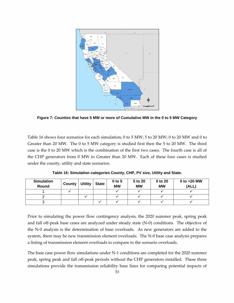
53

: Counties that have W or more of Cumula n the 0 t 5 MW C tegory

Table  four scenarios for ch simulation; 0 to 5  MW;  to 20  and to Greater than 20 MW.  The 0 to 5 MW category is studied first then the  20 hca 20 MW  is   combination of the f ses.   our se is f the  erators  f  0 MW  Greater n 20 M hes ur cases  is studied u , uti and stat

Table 16: Simulation categories County, CHP, PV size, Utility tat

County Util State 5 W

5 to 20 MW

0 to 20 MW

0 to +20 MW (ALL)

Figure 7 5 M tive MW i o a

 16 shows  ea  MW;  20 5 to  0  MW    05 to The f

 MW.  Tth ca

e third  all ose is the 0 to   which the irst two ca

CHP gen rom   to   tha W.   Each of  t e  fonder the county lity  e scenarios.     

and S e.

Simulation Round ity 0 to

M1 2 3

Prio lating  th power  flow contingency analysis,  the 2020 summer peak, spring peak  f peak base ses are  lyzed under steady state (N‐0) conditions.  The objective of  N‐0 analysis  is  the determination of base overloads.   As new generators are added  to  the 

ystem, there may be new transmission element overloads.  The N‐0 base case analysis prepares a listing of transmission element overloads to compare to the scenario overloads. 

The base case power flow simulations under N‐1 conditions are completed for the 2020 summer peak, spring peak and fall off‐peak periods without the CHP generators installed.  These three simulations provide  the  transmission  reliability base  lines  for comparing potential  impacts of 

r  to simu e andthe

all off‐  ca ana

s

54

transmission  reliability.   The  residential PV  resources are  included  in  the base case simulations as previously discussed.   

CHP generator capacity  is  injected  into  the system  in  increments ntil the maximum generation is added or a new transmission element overload occurs under 

ADWP and SDG&E) or a  total of 63 county simulations.    For  each  county  power  flow  simulation,  the  AMWCO  is  recorded  which  is 

AMWCO values are recorded.   There are 72 county simulations for the 5 to 20 MW category. 

  The same power flow simulation process is completed again for the county analysis.  There are a total of 90 county simulations.  The last set of simulations includes all of the CHP generators from 0 to Greater than 20 MW.  Generators are added until either all of the generators are added or until an overload occurs on a transmission element.  The power flow simulation is completed for each county and for the 2020 summer peak, spring peak and fall off‐peak power flow data sets.  There are 93 county simulations for the 0 to Greater than 20 MW.  The total county power flow simulations are 318. 

The next  series of power  flow analyses  is completed  for each utility.   The  individual utilities studied are PG&E, SCE, SDGE, LADWP and IID.     For each utility, the same four scenarios (0 to 5, 5  to 20, 0  to 20 and 0  to Greater  than 20 MW) are completed  for  the 2020 summer peak, spring peak and fall off‐peak.   There are 48 utilities simulations to cover the three seasons and the four different CHP categories. 

The  last  set of power  flow  analyses  is  completed  for  the  entire  state of California.   The  four scenarios are studied for the three data sets.   There are 12 state wide power flow simulations.  

CHP generators on 

For  the county analysis,  the usteady  state  conditions  (N‐0).    The  utility  power  flow  simulation  is  completed  for  the  first contingency (N‐1) conditions for the county being studied.  The first contingency analysis (N‐1) is  the outage of one  transmission  line or one generator.   The  total number of contingencies  in each simulation  is dependent upon  the utility and ranges  from 200  to over 5,000 simulations.  As  shown  in  Table  15,  there  are  21  county  power  flow  simulations  for  each  of  the  three simulation periods  (14  in PG&E, 5  in SCE, 1  in L

described in the next section. 

Continuing with the county analysis, the next set of power flow simulations includes only those CHP generators  in the 5 to 20 MW category.   The CHP generators are  incrementally added  in each  county  until  all  of  the  generators  are  installed  or  an  overload  occurs  in  one  or more transmission  elements  under N‐0  conditions.   A  utility  power  flow  contingency  analysis  is completed for each  individual county scenario.   The 

The next set of simulations includes all generators from 0 to 20 MW, or the first two scenarios.

55

The power flow simulations for county, utility and state for the three seasons are 378.  The full list of combinations is shown in Table 17 below. 

Table 17: MW of CHP in each California County

PG&E SCE

COUNTY 0 -5 MW 5 – 20 MW 0 - 20+ MW COUNTY 0 -5 MW

5 – 20 MW

0 - 20+ MW

ALAMEDA 15 35 50 KERN 0 0 159 BUTTE 0 11 11 LOS ANGELES 126 113 1433

CONTRA COSTA 7 6 177 ORANGE 28 28 56 FRESNO 15 19 93 RIVERSIDE 11 0 11

HUMBOLDT 11 10 133 SAN BERNARDINO 10 43 94

KERN 0 37 37 TULARE 0 0 114 LASSEN 0 11 11 VENTURA 10 18 52 KINGS 0 7 7 SDG&E

MADERA 6 9 73 COUNTY 5 – 20 MW

0 - 20+ MW

0 -5 MW

MENDOCINO 14 30 0 16 156 SAN DIEGO 16 MERCED 12 42 301 LADWP

MONTEREY 0 7 48 COUNTY 0 -5 MW

5 – 20 MW

0 - 20+ MW

PLACER 0 11 11 LOS ANGELES 38 0 1705 SACRAMENTO 12 6 18 IID

SAN JOAQUIN 25 13 63 COUNTY 0 -5 MW

5 – 20 MW

0 - 20+ MW

SANTA CLARA 15 17 32 IMPERIAL 0 0 114 SANTA CRUZ 0 16 16

SHASTA 0 4 4 SOLANO 7 0 123 SONOMA 5 0 5

STANISLAUS 12 32 103 TEHAMA 9 0 9

YOLO 5 0 5  

56

5 RESULTS

5.1 2010 RESULTS  

The  objectives  of  the  2010  a   are: Determine  if  the  existing  CHP  improved  grid reliability;  and  (2)  ide m c g te s.      Energy  and Environmental  Analysis,  Inc   provided  th   d the line  database.    A combination of map  a bu istin  a W  su 10 r flow case is used to assign the CHP f es to er fl us.    t c e cl bus with  load and generation is used  sent  CHP facility.    

For each substatio HP,  MWs HP a mbin  CHP resources re load reducers so the bus loads are net load.  For this analysis, CHP load and generation are 

ns.   The  locations  are plotted 

nalysis  a  bench

  (1) ark  for Prov omparin   2020  al rnative

.  (EEA) e  CHP ata  via  ir  ons and s load l g from ECC mmer 20  poweaciliti  a pow ow b In mos ases, th osest 

to repre the 

n with C  the aggregated  of C re co ed.  Thearepresented  several ways.   When a CHP  resource  is added  to a bus  there  is a corresponding load added to the bus equal to the CHP resource.  When the CHP is simulated out of service for a contingency case, then the load at the substation automatically increases since the CHP is not available  to  reduce  load.    This  representation  simulates  the  impacts  that  CHP  provides  by reducing load on substations and transmission lines. 

The  figure  below  shows  the  locations  of  the  2010  existing CHP  locatioby city, and the size of the circle indicates the range of MW the site produces.   

57

ons  

Figure 8: 2010 Existing CHP Locations cumulative MW by city

Power  flow simulations are completed  for  three 2010 seasons: spring peak, summer peak and fall off peak.  There are two power flow N‐1 contingency simulations completed for each utility (PG&E, SDG&E, IID, LADWP, and SCE) and all of California combined.   The two simulatiare with (BASE AMWCO) and with (CHP AMWCO).  For each simulation, the AMWCO, deltaAMWCO and RTBR are calculated and shown in Table 18.  The 2010 RTBR are all negative for each utility and state‐wide except  for  IID.   The negative RTBR values  indicate a  transmission benefit in reducing transmission congestions with the addition of CHP.   

Table 18: Existing CHP Resource RTBR Values for 2010

Base AMWCO

CHP AMWCO CHP IN DELTA RTBR Summer

CA 29,843 7,204 8,813 -22,639 -2.6

PGE 21,900 4,467 5,885 -17,432 -3

SCE 5,670 2,196 1,738 -3,474 -2

SDGE 1,103 0 442 -1,103 -2.5

IID 249 249 8 0 0

LADWP 3,201 249 742 -2,952 -4

Spring Base

AMWCO CHP

AMWCO CHP IN DELTA RTBR CA 17,027 4,350 8,813 -12,677 -1.4

58

PGE -2.1 15,486 3,121 5,885 -12,365

SCE 1,593 883 1,738 -711 -0.4

SDGE 4 0 442 -4 0

IID 265 2 69 8 4 0.6

L 44 742 34 ADWP 2,578 -2,5 -3.4

Fall Base

AMWCO

CHP

AMW P IN TA R CO CH DEL RTBCA 16,025 2,28 ,813 6 9 8 -13,73 -1.6

PGE 16,121 1,7 885 -14,416 05 5, -2.4

SCE 5,670 262 1,738 -5,408 -3.1

SDG 6 15 E 1 442 -1 0

IID 441 45 8 1 10 1.3

L 0 742 0 ADWP 560 -56 -0.8

Figure 3 displays th or three d 2010 seasons in graphical form.  The utility results for PG&E, SCE nd LADWP icati t the CHP resources provided a benefit  syste ucing  MW  2010 spring and fall CHP resources not exhibit  benefit.   This  be attributed  to low  load  levels  an   flows.  e  7.5 M CHP rce  in  the  Imperial Irrigation District (IID positive RT  in all  asons

Figure 9: 2010 CHP Comparison of RTBRs

The statewide California results for 2010 CHP is not surprising.  For all three seasons, the RTBR is negative.  With CHP facilities being represented in each utility, collectively, this reduces the congestion on the grid and enhances overall grid reliability and stability.     

e RTBR values f ifferent , SDG&E, a  are all negative ind ng tha

 to the transmission m by red the A CO.  The  for SDG&E did   a dramatic  couldd/or  interchange   The  on W    resou

) produced  BR values 3 se .    

‐6

‐4

‐2

0

CA PGE SCE SDGE IID LADWP

2010 CHP Comparison of RTBRs2

Summer Spring Fall

59

5.2  

The 2020  separated by the  density  counties  are defined by the with less than 1,000 people   city within the county  completed by county, utility  in PG&E, 5 in SCE and 

5.2.1 2020 Sum 

igh  negative  RTBR’s  in  Sacramento, 

not completed.   Alameda had a high RTBR benfit  ratio  for  the 0  to 5 MW category.  Fresno County    

2020 RESULTS

summer peak, spring peak, and fall off peak county results are of  the  population,  and  classified  as  rural  or  urban.    Rural  Bureau of the Census by population density [1].  Counties per square mile are rural, and greater  than  this, with a major

lines, are defined as Urban.  The 2020 power flow analyses are  and entire state of California.  There are 14 counties studied

one each in SDG&E and LADWP areas.     

mer County Results

The  results  are  organized  by  county,  and  filtered  from  most  beneficial  (highest negative)  to most detriment  (highest positive) RTBR’s.   The  results are plotted  in  the following figures for PG&E, SCE and the remaining utilities.  The Summer PG&E RTBR results are presented in Figure 4 and Table 19 for the “Urban” counties of PG&E for the four categories (0 to 5 MW, 5 to 20 MW, 0 to 20 MW and 0 to Greater than 20 MW).   

In  the  PG&E  urbanized  counties,  there  are  hAlameda,  Fresno  counties  for  certain  category  sizes.    Sacramento  County  has  the highest benefical RTBRs  for  the 0  to 5 MW, 5  to 20 MW and 0  to 20 MW  categories.  There  are no  single CHP units  greater  than  20 MW proposed  in  Sacramento  so  that analysis  is 

 has high RTBR ratios for all four categories.

60

19 R or reas

UR COUNTIES

Table : RTB Results f PG&E Urban A

PGE BAN

COUNTY Categor RTy CHP MW BR

S NT TO 5 -ACRAME O 0 12 3.1 S NTO O 2 -2ACRAME 0 T 0 18 .6

ALAMEDA TO 5 -10 15 .67 S NTO O 20 -1ACRAME 5 T 6 .6

FRESNO TO 5 -10 15 .51 FRESNO O 20 -15 T 19 .46 FRESNO 0 TO 20 34 -1.38 FRESNO 0 TO 20+ 93 -0.87

SANTA CLARA 0 TO 5 15 -0.6 SANTA CLARA 5 TO 20 17 -0.6 SANTA CLARA 0 TO 20 32 -0.6

ALAMEDA 0 TO 20 50 -0.09 CONTRA COSTA 0 TO 20+ 197 -0.02 CONTRA COSTA 0 TO 20 13 0.16 CONTRA COSTA 0 TO 5 7 0.2 CONTRA COSTA 5 TO 20 6 0.38

ALAMEDA 5 TO 20 35 0.46  

The RTBR results can be easily seen  in Figure 4 below.   Although Santa Clara County has a negative RTBR, the value is low compared to the more beneficial areas. 

61

Fi 20 Sum rba nti

As discussed before, th ere   into  n a al.   Table 20 displays the RTBR  results  for  th s.   T ties  are st  locations  for CHP resources are San Joaqu , Stanislaus, Merc lac  Kings Counties.  The RTBR benefits in all cate  San Cou ny lopment in any of the categories  is benefical  to seve   the best RTBR,  the category providing the best R nefits is th MW.  e 5 t W category provides the best RTBR benefits to Ki lacer Cou

The  two  counties with  p indicating  that  the ion  of CHP  is  a detriment  to transmission  reliability  are o  and      T ”    that  the  full  CHP potential  could not  be    even ll CH enet   caused  transmission congestion. 

s for the PG&E R Cou

PG&E RURAL COUNTY C BR E R

U egory CHP MW

RTBR

gure 10: 20 mer PGE U n cou es

e CHP resources w divided urba nd rure PG&E  rural area he coun that    the bein, Sonoma, Solano ed, P er andgori ed in San  County.

es occurr         Joaquin n A

nty.    deve

  Joaquin In  the  counties withTBR be e 0 to 5   Th o 20 M

ngs and P nties. 

ositive RTBR    addithe  “* Mendocin Hunboldt. indicates

installed  and  that   a  sma P p ration

Table 20: RTBR Result ural nties

ategory MW RTCHP COPG& URAL

NTY Cat

SAN JOAQUIN 0 to 5 25 -3.42 MERCED 5 to 20 42 -0.43 SONOMA 0 to 5 5 -2.74 MERCED 0 to +20 301 -0.36

SAN JOAQUIN 0 to 20 38 -2.37 SANTA CRUZ 5 to 20 16 -0.29 SOLANO 0 to 5 7 -2.09 KERN 5 to 20 37 -0.26

SAN JOAQUIN 0 to +20 63 -1.92 MADERA 0 to +20 73 -0.25 SAN JOAQUIN 5 to 20 13 -1.48 MONTEREY 5 to 20 7 -0.1 STANISLAUS 0 to 5 12 -1.26 MADERA 5 to 20 9 -0.04

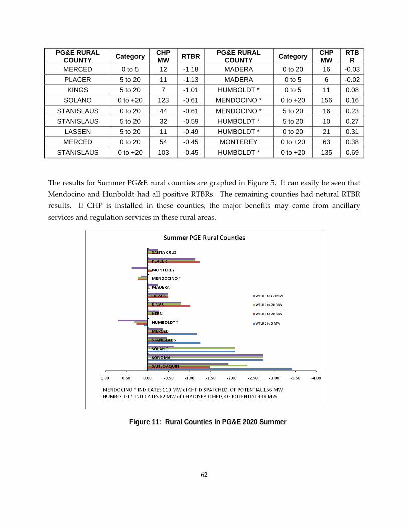
62

PG&E RURAL COUNTY

CHP MW

RTBR Category CHP

MW RTBR PG&E RURAL COUNTY Category

MERCED 16 -0.03 0 to 5 12 -1.18 MADERA 0 to 20 PLACER 6 -0.02 5 to 20 11 -1.13 MADERA 0 to 5 KINGS 11 0.08 5 to 20 7 -1.01 HUMBOLDT * 0 to 5

SOLANO 156 0.16 0 to +20 123 -0.61 MENDOCINO * 0 to +20 STANISLAUS 16 0.23 0 to 20 44 -0.61 MENDOCINO * 5 to 20 STANISLAUS 10 0.27 5 to 20 32 -0.59 HUMBOLDT * 5 to 20

LASSEN 21 0.31 5 to 20 11 -0.49 HUMBOLDT * 0 to 20 MERCED 63 0.38 0 to 20 54 -0.45 MONTEREY 0 to +20

STANISLAUS 135 0.69 0 to +20 103 -0.45 HUMBOLDT * 0 to +20

The results for Summer PG& 5.  It can easily be seen that 

Figure 11: Rural Coun G&E 2 Sum

E rural counties are graphed in Figure Mendocino and Hunboldt had all positive RTBRs.   The remaining counties had netural RTBR results.    If  CHP  is  installed  in  these  counties,  the major  benefits may  come  from  ancillary services and regulation services in these rural areas.   

ties in P 020 mer

63

Even    fewer counties   in Los   area.  Los    in  the table 

Table    of  the scenarios  other utilities, served  by LADWP resources are 

Table 21: 2020 ornia Utilities

when  combined  together,  SCE,  IID,  LADWP  and  SDG&E  have  significantly with potential CHP resources  than PG&E.   The  total megawatts of CHP resources

Angeles County are 3,138 MW that is more than all of the CHP resources in the PG&EAngeles County  is served by both SCE and LADWP and  is  therefore shown  twicebelow. 

21  displays  the RTBR  results  for  the  southern California  utilities.    For  SCE,  all have beneficial  results although  the RTBR values do not exceed  ‐1.0.   For  the  the  RTBR  are  all  small  negative  values  except  for  Los  Angeles  County  that has a RTBR of 0.63.   The RTBR values are so small that installing CHP 

neither beneficial nor detrimental to the transmission system.    

Summer Urban RTBR for Southern Calif

SCE URBAN

COUNTIES

COUNTY Category CHP MW RTBR

Los Angeles (SCE) 5 to 20 113 -0.97 Los Angeles (SCE) 0 to 20 239 -0.91 Los Angeles (SCE) 0 to 5 126 -0.87

Orange 0 to 5 28 -0.32 Los Angeles (SCE) 0 TO 20+ 1,433 -0.3

Orange 0 to 20 56 -0.26 Orange 5 to 20 28 -0.25

Riverside 0 to 5 11 -0.13 Other Utilities

COUNTY Category CHP MW RTBR

San Diego (SDGE) 5 to 20 14 -0.75 San Diego (SDGE) 0 to 20 30 -0.53 San Diego (SDGE) 0 to 5 16 -0.47

Los Angeles (LADWP) 0 to 5 38 -0.27 Imperial (IID) 0 TO 20+ 114 -0.02

Los Angeles (LADWP) 0 TO 20+ 1,705 0.63  

Figure  6  below  shows  the  RTBR  for  all  of  for  the southern California utilities.  The RTBR scale does not exceed ‐1.0.   

the  2020  summer  urban  CHP  scenarios 

64

Figure 12

SCE is the only southern California utility with Figure 7.    The  installation  of  CHP  resources  produce   and Ventura Counties.  The RTBR values for the remaining CHP scenarios are neither beneficial nor dthan the 0 to 5 MW has a significant impact on the transmission system.     

Table 22: 2020 RTBR Rural County Results for Southern California Utilities

: Summer SCE Urban counties

 rural counties as shown on Table 22 and s  positive  RTBR  values  in  Kern,  Tulare,

etrimental.  Ventura County has the highest positive RTBR values.  Any CHP scenario greater 

SCE RURAL COUNTIES

COUNTY Category CHP MW RTBR

San Bernardino 0 to 5 10 -0.49 Ventura 0 to 5 10 -0.18

San Bernardino 5 to 20 43 -0.17 San Bernardino 0 to 20 53 -0.16

Tulare 0 TO 20+ 114 0.84 Kern 0 TO 20+ 159 1.53

San Bernardino 0 TO 20+ 94 2.39 Ventura 0 TO 20+ 52 6.07 Ventura 0 to 20 28 11.54 Ventura 5 to 20 18 17.99

65

ties

The county results are p ically f hole  e for  er, by size range 0 to 5 MW,  red  indicates  a in  th   county,  yel neutral,  and  blue  is detrimental (Figure 8).  e cou er did t hav CHP or did not have any in the category cons

Figure 13: Summer SCE rural coun

lotted geograph or the w stat Summ  beneficial  effect  e marked low  is White indicates th nty eith  no e any idered. 

66

5.2.2 2020 Spring County Results  Th  s  f BR  a for  er siRTB re displayed  bot ular and graph The spring  data  have droelec erat wi alifo gh  i from   Pacific Nort m  hydroelectric  power  purchases.    T nia  sys ds  a low  there  r air conditioning no eatin s. 

As  23,  County  high R of   the to 5  scen tra Cost ty h  hi itive    for  Gr r  tha  M  the  ena  the llation esourc uce   tra efits r th nar iscus

Figure 14 Summer RTBR all California counties for 0 to 5 MW (Top LHS), 5 to 20 MW (Top RHS), 0 to 20 MW (Bottom LHS), and All (Bottom RHS)

e formats for theR results a

pring and all RTh tab

 results re the same as ical form.  

the summ  analy flow

s.  The  in  power  sets

  high  hy tric  gen ion  thin  C rnia  and  hi mports    thehwest  fro he Califor tem  loa re    sinceis neithe r h g load

 shown  in Table  Alameda has a   negative RTB   ‐1.32 for  0   MWario.   Con a Coun as a gh pos RTBR of 1.97   the 0  to eate n 20

W scenario.   In other sc rios,   insta  of CHP r es prod no significantnsmission ben  except fo e sce ios d sed above.   

67

3: 2 PG ing esu

Table 2 020 &E Spr Urban RTBR R lts

PGE URBAN

COUNTIES

COUNTY Category CHP MW RTBR

ALAMEDA 0 TO 5 15 -1.32 FRESNO 0 TO 5 15 -0.54

ALAMEDA 0 TO 20 50 -0.43 SACRAMENTO 0 TO 20 18 -0.39 SACRAMENTO 0 TO 5 12 -0.36

CONTRA COSTA 0 TO 20 13 -0.28 SACRAMENTO 5 TO 20 6 -0.2 SANTA CLARA 0 TO 5 15 -0.18

CONTRA COSTA 5 TO 20 6 -0.14 CONTRA COSTA 0 TO 5 7 -0.11 SANTA CLARA 5 TO 20 17 -0.1 SANTA CLARA 0 TO 20 32 -0.1

ALAMEDA 5 TO 20 35 -0.08 FRESNO 5 TO 20 19 0.03 F 0.03 RESNO 0 TO 20 34 FRESNO 0 TO 20+ 93 0.06

CONTRA COSTA 0 TO 20+ 197 1.97  

Figure  9  compares  the  2020  spring  PG&E  urban  RTBR  results  in  graphical  form.    The  two extreme scenarios for Contract Costa and Alameda Counties can be easily seen as compared to the other scenarios. 

68

The RTBR  .   Kern and Placer Coun high negative RTBR  value Mendocino Counties   results.   

PG&E RUCOUNTY RTBR

Figure 15: Spring PG&E Urban Counties

results for the PG&E rural counties are shown  in Table 24 and Figure 9ties are consistent with the summer results in that these counties have s  and  remain  good  areas  for  CHP  development.    Humboldt  and 

continue to have positive RTBR values that are consistent with the summer

Table 24: PG&E 2020 Spring RTBR by County

RAL Category CHP

MW RTBR PG&E RURAL COUNTY Category CHP

MW KERN -0.07 5 to 20 37 -2 MADERA 0 to +20 73

PLACER -0.04 5 to 20 11 -1.19 MONTEREY 5 to 20 7 MADERA -0.03 0 to 5 6 -0.74 MADERA 5 to 20 9

KINGS -0.02 5 to 20 7 -0.73 MERCED 5 to 20 42STANISLAUS -0.02 0 to 5 12 -0.61 SANTA CRUZ 5 to 20 16

MADERA 0 to 20 16 -0.48 SOLANO 0 to +20 123 0 MERCED 0 to 5 0 to 20 54 0 12 -0.37 MERCED

STANISLAUS 0 to 20 44 -0.2 LASSEN 5 to 20 11 0.01 STANISLAUS 0 to +20 103 -0.2 MONTEREY 0 to +20 63 0.03 SAN JOAQUIN 5 to 20 13 -0.18 MERCED 0 to +20 301 0.05 SAN JOAQUIN 0 to 5 25 -0.17 MENDOCINO * 0 to +20 156 0.09

SONOMA 0 to 5 5 -0.12 MENDOCINO * 5 to 20 16 0.14 SAN JOAQUIN 0 to 20 38 -0.12 HUMBOLDT * 5 to 20 10 0.61

SOLANO 0 to 5 7 -0.12 HUMBOLDT * 0 to 20 21 0.67 STANISLAUS 5 to 20 32 -0.09 HUMBOLDT * 0 to 5 11 0.71

69

MW COUNTY MW PG&E RURAL

COUNTY Category CHP RTBR PG&E RURAL Category CHP RTBR

SAN JOAQUIN 0 to +20 63 -0.07 HUMBOLDT * 0 to +20 135 1.33

The  SCE,  Table  25  and Figure 10.   RTBR values vary between benefical or detrimental

Figure 16: Spring PG&E rural counties

IID,  LADWP  and  SDG&E  urban  spring  RTBR  results  are  shown  in The spring urban results are consistent with the summer results.  The  0 and ‐0.5 for all scenarios.  The injection of CHP resources are neither 

 to transmission grid reliability.  

Table 25: 2020 Spring Southern California Urban RTBR Results

SCE

URBAN COUNTIES

COUNTY Category CHP RTBR MW Los Ang eles (SCE) 5 to 20 113 -0.5Los Angeles (SCE) 0 to 20 239 -0.24

Orange 0 to 5 28 -0.08 Orange 0 to 20 56 -0.04

Los Angeles (SCE) 0 to 5 126 -0.03 Riverside 0 to 5 11 -0.03

SCE URCO

BAN

UNTIES

COUNTY Category CHP MW RTBR

Orange 5 to 20 28 -0.01 Los Angeles (SCE) 0 TO 20+ 1,433 0.15

Other Utilities

COUNTY Category CHP MW RTBR

Imperial (IID) 0 TO 20+ 114 -0.02 San Diego (SDGE) 5 to 20 14 0 San Diego (SDGE) 0 to 20 30 0 San Diego (SDGE) 0 to 5 16 0

Los Angeles (LADWP) 0 to 5 38 0 Los Angeles (LADWP) 0 TO 20+ 1,705 0

Ventura County has high positive RTBR results but  in the spring RTBR results, the values are P resources have a detrimental impact during the summer 

eak period but a beneficial impact in the spring period.  Because of the extremely high positive 

Figure 17: Spring SCE Urban Counties

The SCE rural county RTBR results are shown in Table 26 and Figure 12.  In the summer results, 

negative.  This indicates that the CHpRTBR values  in  the summer as compare  to  the RTBR spring values,  the spring results do not change  the  CHP  value  in  improving  transmission  grid  reliability.    The  injection  of  CHP resources in San Bernardino County produces negative RTBR values except for the 0 to Greater 

70

than 20 MW  scenario.   The  injection of CHP  resources greater  than 20 MW  is detrimental  to transmission reliability.      

Table 26: 2020 SCE Rural County RTBR Results

71

COU SCE

RURAL NTIES

COUNTY CaCHMW RTBR tegory

P

Ventura 5 18 -2.to 20 2 Ventura 0 28 -1.4 to 20 1 Ventura 0 TO 52 -0.7 20+ 6

San Bernardino 0 10 0 to 5 Ventura 0 10 0 to 5 Tulare 0 T 11 0 O 20+ 4

Sa ino 5 t 43 0.0n Bernard o 20 1 Sa ino 0 53 0.0n Bernard to 20 1

Kern 0 T 159 0.3O 20+ 6 Sa ino 0 T 94 1.8n Bernard O 20+ 9

Figure 18: 2020 SCE Rural County RTBR Results

he county results are plotted geographically for the whole state for Spring, by size range 0 to 5 MW,  red  indicates  a  beneficial  effect  in  the marked  county,  yellow  is  neutral,  and  blue  is etrimental (Figure 14). White indicates the county either did not have any CHP or did not have  in the particular size category considered. 

T

dany

72

Fig ng RTB liforni ount 0 to 5 LHS), W ( (B tom LH and All (Botto

5.2 Fall Co sult 

The r flow  ress  yst ce th  is a l peri 2 am rning) ystem ads   min   hydr   ge tion t min ce  the  r rs are the  t  leve eration ‐line    the  

ure 19 Spri R all Ca a c ies for MW (Top 5 to 20 M Top RHS), 0 to20 MW ot S), m RHS)

.3 2020 unt Re s

 fall powe results st the s em sin e time period  fall off‐peak fal od (  in  the mo .    The  s   lo are  at imum,  the oelectric nera   is  aimum sin eservoi  at  lowes ls, PV gen   is off and re are

73

h sfers between  th ert Southwe ific Northwest. e 27 and Figu  the  lts  e f E rur s. 

27: PGE ban C su

P BAN C NTY Cate W

igh power  tranre 14 show

e Desfor th

st and  the Pacal countie

   TablRTBR resu all PG&

Table 2020 Ur ounty RTBR Re lts

G&E UR OU gory CHP M RTBRALAMED 0 A -5 15 0.08 ALAMED 5 -A 20 35 0.23 ALAMED 0 -A 20 50 0.24 ALAMEDA 0 - +20 50 0.24

CONTRA COSTA 0 -5 7 0.21 CONTRA COSTA 5 - 20 6 0.24 CONTRA COSTA 0 - 20 13 0.11 CONTRA COSTA 0 - +20 177 4.76

FRESNO 0 -5 15 -1.02 FRESNO 5 - 20 19 -1.01 FRESNO 0 - 20 34 -1.06 FRESNO 0 - +20 93 -0.69

SACRAMENTO 0 -5 12 0.39 SACRAMENTO 5 - 20 6 0.68 SACRAMENTO 0 - 20 18 0.50 SACRAMENTO 0 - +20 18 0.00 SANTA CLARA 0 -5 15 0.06 SANTA CLARA 5 - 20 17 0.06 SANTA CLARA 0 - 20 32 0.02 SANTA 0.02 CLARA 0 - +20 32

Figure 20: 2020 PGE Urban County RTBR Results

74

In  the 2020 Fall Case,  the county  to benefit  fro P  is Fresno County.   Fresno contains all sizes of CHP.    detrimen s to  ot an county in PG&E area.   Contra Costa  is tally a   in Fa ban  &E  counties and has CHP resources in all of

Table 28 and Figure  ults f fall PG&E rural  nties.  Kern, Madera and  King  Counties  ate nef   all  t e  seasons  in  certain scenarios as shown below and Me unt ontin  have positive RTBR dicating that any CHP development causes transmission problems in the counties.  Humboldt 

cating  that  the CHP  injection has  little  impact on transmission reliability.  

Table 28: PG&E 2020 Rural County RTBR Results

PG&E RURAL COUNTY Catego

HP RTBR

RURAL UNT y

CHP MW RTBR

 only urban  m CH everyThere are  tal impact her urb

  the most detrimen ffected ll, Ur PG the categories.  

15 show the RTBR res or the  coucontinue  to  demonstr   RTBR  be its  for hre

.  Humboldt  ndocino co ies c ue toinCounty  did  not  have  the  full  potential  of  CHP  resources  dispatched  due  to  transmission overloads; 92 MW out of 448 MW  in Humboldt County.   The remaining counties continue  to have RTBR values  that are close  to zero  indi

ry MWC

COPG&E

Y CategorKERN 5 to 20 -2.28 OAQ 38 0.06 37 SAN J UIN 0 to 20

MADERA 5 to 20 -2.18 LAN 123 0.06 9 SO O 0 to +20MADERA 0 to +20 -2.07 A CR 16 0.07 73 SANT UZ 5 to 20MADERA 0 to 20 -1.77 NOM 5 0.09 16 SO A 0 to 5

KINGS 5 to 20 -1.36 NISLA 12 0.1 7 STA US 0 to 5MADERA 0 t -1.32 LACER 5 to 20 11 0.1 o 5 6 P MERCED 0 to -0.44 NTER 0 to +20 63 0.1 +20 301 MO EY MERCED 5 to 20 -0.4 RCE 0 to 5 12 0.11 42 ME D MERCED 0 to 20 -0.31 OLANO 7 0.12 54 S 0 to 5

‐2.00‐1.1.02.004.005.006.00

ALAMEDA

CON ST

FRES

R NT

A TA CLARAPGE Urb u ties

000.0003.00

TRA CO A

NO

SAC AME O

San Co NnFall 0 ‐+…

75

PG&E RURAL COUNTY Category

CHP MW RTBR

PG&E RURAL COUNTY Cat

CHP MW RTBR egory

LASSEN 5 to 20 11 0 SAN JOAQUIN 5 to 20 13 0.13 STANISLAUS 0 to 0 DOCIN * 0 to +20 156 0.32 +20 103 MEN O STANISLAUS 0 to 0.01 OCIN 16 0.54 20 44 MEND O * 5 to 20MONTEREY 5 to 20 0.01 OLD 0 to 20 21 1.61 7 HUMB T *

STANISLAUS 5 to 20 32 0.04 HUMBOLDT * 0 to 5 11 1.68 SAN JOAQUIN 0 to +20 63 0.05 HUMBOLDT * 5 to 20 10 1.68 SAN JOAQUIN 0 to 5 25 0.06 HUMBOLDT * 0 to +20 135 2.28  

ral counties Figure 21: Fall PG&E Ru

Table 29  shows  the RTBR  results  for  the SCE,  IID, LADWP and SDG&E urban  counties.   As shown in the table, the RTBR values are close to zero for all of the counties indicating that the CHP resources have little impact on transmission reliability.  The RTBR values are so small that the results are not graphed. 

Table 29: Southern California

SCE CO

Utilities Urban RTBR Results

URBAN

UNTIES

COUNTY Category CHP MW RTBR

Los Angeles (SCE) 0 to 5 126 -0.06 Los Angeles (SCE) 0 to 20 239 -0.03 Los Angeles (SCE) 0 TO 20+ 1,433 -0.01 Los Angeles (SCE) 5 to 20 113 0

Orange 0 to 5 28 0 Orange 0 to 20 56 0 Orange 5 to 20 28 0

Riverside 0 to 5 11 0 Other Utilities

COUNTY Category CHP MW RTBR

San Diego (SDGE) 5 to 20 14 0 San Diego (SDGE) 0 to 20 30 0 San Diego (SDGE) 0 to 5 16 0

Los Angeles (LADWP) 0 to 5 38 0 Los Angeles (LADWP) 0 TO 20+ 1,705 0

Imperial (IID) 0 TO 20+ 114 0.5

Table 30 shows the RTBR results for the SCE rural counties.  The RTBR values are also close to zero for all counties.  Since the values for the southern California urban and rural counties are so low, a graphical display is not developed. 

Table 30: SCE Counties 2020 RTBR Results

SCE RURAL COUNTIES

COUNTY Category CHP MW RTBR

Tulare 0 TO 20+ 114 -0.01 Ventura 0 TO 20+ 52 -0.01 Ventura 0 to 20 28 -0.01 Ventura 5 to 20 18 -0.01

San Bernardino 0 to 5 10 0 San Bernardino 0 to 20 53 0

Kern 0 TO 20+ 159 0 Ventura 0 to 5 10 0.01

76

SCE RURAL COUNTIES

COUNTY Category CHP MW RTBR

San Bernardino 5 to 20 43 0.01 San Bernardino 0 TO 20+ 94 0.34

The county results are plotted geographically  for  the whole state for Fall, by size range 0  to 5 MW,  red  indicates  a  beneficial  effect  in  the marked  county,  yellow  is  neutral,  and  blue  is detrimental (Figure 18). White indicates there was either no CHP in that county or none in the category considered. 

77

78

Figure 22 (Top RHS), 0 to 20

sion reliability results (RTBR) are displayed in graphical form for each utility, and size category  of  CHP, first  (Figure  17) followed by SCE (Figure 21). 

Figure 23: Summer, Spring and, Fall PGE CHP Categories

: Fall RTBR all California counties for 0 to 5 MW (Top LHS), 5 to 20 MWMW (Bottom LHS), and All (Bottom RHS) California Utility Results

The simulations are conducted at the utility  level as per simulation Round 2  in Table 16.   The transmis

  for  2020  Summer,  Spring  and  Fall.  PG&E  is  presented  (Figure 18), LADWP (Figure 19), IID (Figure 20), and SDG&E 

79

  also  beneficial  to  PG&E  in  the  summer  cases,  but  not  as  beneficial  as  the  other smaller categories  all generation dispatched, and

In  the 2020   5  to 20 MW category and the dispatched in each category.    When MW  total),  the transmission 

In the fall season, categories of CHP.   

In SCE, the only  the 0 to 5 MW category which the  0  to  20 MW category,  the   category,  the impact  reduces, spring,  there  is  a transmission  r  than  20 MW category.  There is es. 

In  the 2020 summer peak, PG&E experiences a  transmission grid benefit  from  the addition of CHP  in every CHP  category.     The most beneficial  size  category  for PG&E  is  the 0  to 5 MW followed by the 0 and 20 MW category.  Combining all the units in the 0 to Greater than 20 MW category  is

 with no units greater than 20 MW, with a RTBR of  ‐0.2, with ‐1.2, with just the 0 to 5 MW category.    

spring,  there  is a  transmission benefit  from  the 0  to 5 MW category, 0 to 20 MW category, with 191 MW, 309 MW and 500 MW   the  Greater  than  20  MW  category  is  dispatched  (1,521 

reliability decreases with a RTBR of positive 0.1.   

 there is no benefit to transmission reliability for any of the 

 transmission grid benefit in all three seasons is the dispatch of  has  a RTBR  of  ‐0.7.    In  both  the  5  to  20 MW  category  and 

summer RTBR are.   With  the  inclusion of  the Greater  than 20 MW  but  there  is  still  a  slightly  positive  RTBR.    In  the  2020 

benefit  from  all  of  the CHP  categories  except  for  the  0  to Greate minimal transmission impact from CHP generators in all cas

Figure 24: Summer, Spring and, Fall SCE CHP Categories

80

  transmission benefits  for any other catego

he  addition  of CHP  generation  in  the  IID  area  resulted  in  no  benefits  for  any  category  or season. 

Figure 26: Summer, Spring and, Fall IID CHP Categories

For  the  LADWP  2020  summer  peak,  the  dispatch  in  the  0  to  5 MW  category  results  in  a transmission benefit of a negative RTBR of  ‐0.25.   There are no

ry or season.   

Figure 25: Summer, Spring and, Fall LADWP CHP Categories

T

81

There gory in SDG&E 5 to 20  categ    of  shows a transmissio   on   SDG     other seasons.   

Figure 27 CHP gories

5.2.4 All of ornia Results  

Simulations are  repeated  for  the entire state of California  includ ll  the m tilities and each CHP ge eratio  results are presented in Figure 22. 

For  the summer peak, every CHP category prov transmiss nefit, w  counties and  utilitie   com his  indicates  the  counties which  are detrimentally  affected  are offset by the  enefic d counties.  The m eneficial C tegory   0 to 5 MW category, 452 MW is  a RTBR .0 in Summ small positive of 0.07 in Spring and a negative   ‐0.03 Fall.    In  the  fall,  there  is  little  transmission benefit  to adding CHP,  r  v all or neutral RTBR mov towards  sitive RTBR for the la  ca

The  5  to  20    ca enefi to  the  g Summer  pring, w  MW  in Summer and 632 MW  both  negati Rs.  In summer, the resultant RTBR for the 5  to 20 MW category 7, an  Spring  it  is  ‐0.4.    In Fall 632 MW  in  the 5  to 20 MW category  is  ispat pri ut  it  results in  a  detrimental  RTBR 0.14.    The 

 are no CHP generators in the Greater than 20 MW category.  The most beneficial cate is the n  benefit

 MW  the

ory with a negative RTBRsummer  but  no

 ‐0.75.  Overall  benefit  during

 the RTBR  any  of  theE  grid  in

: Summer, Spring and, Fall SDG&E Cate

Calif

ing a ajor un n category. The

ides a  ion be hen alls  are bined.   Tb 

ially affecte ost b HP ca is the installed resulting RTBR of

 in  in 

 of ‐1 er, a   the esult is either a ery sm ing  a po

rger MW tegories.   

MW 

tegory  is  b cial  rid  in  and  S ith  484 in Spring,  is  ‐0.0

 gived  in

ve RTB

d ched  as  in  S ng,  b     of 

82

 in Summer nd Spring, with negative RTBR’s of ‐0.5, and ‐0.2 respectively.   

In  Spring,  dispatching  4, ssible  without  additional transmission overloads), results in a detrimental effect shown by a positive RTBR of 0.1.  It was possible to dispatch 5,030 MW i steady state overloaded lines but the resultant RTBR is positive ately 0.4. 

The overall RTBR results  for e CHP category are shown  in Table 31for each of the utilities and  the entire state of California.     red areas  indicate negative RTBRs, where 

combination of the 0 to 5 MW category and 5 to 20 MW category is beneficial againa

Figure 28: Summer, Spring and Fall analysis for all CHP categories

As in the 5 to 20 MW category, the RTBR in Fall is positive and results in a RTBR of 0.05.  When all available CHP is dispatched in Summer (0 to greater than 20 MW) the result is beneficial in Summer.   

119  MW  (the  maximum  amount  po

 of CHP in Fall, w thout additional  at approxim    

ach season and  The

inserting more CHP generation provides transmission benefits.  The blue areas indicate positive RTBRs where  inserting more CHP generation  is detrimental and  the yellow areas are neutral, where there is no effect, or no generation dispatched.   

Table 31: All of 2020 California results, split by season and size of installed generation

Utility Cat. CHP MW RTBR Summer RTBR Spring RTBR Fall Summer

83

PGE 0 to 5 MW 197 -1.18 -0.17 0.15

5 to 20 MW 309 -0.78 -0.67 0.65

0 to 20 MW 506 -0.98 -0.50 0.36

ALL CHP MW 1473 -0.26 0.14 1.72

LADWP 0 to 5 MW 38 -0.27 0.00 -0.04

5 to 20 MW 0 0.00 0.00 0.00

0 to 20 MW 38 -0.27 0.00 -0.02

ALL CHP MW 1705 0.63 0.00 0.01

W 0 0.00 0.00 0.00 IID 0 to 5 M

0.00 5 to 20 MW 0 0.00 0.00

0 to 20 MW 0 0.00 0.00 0.00

ALL CHP MW 106 -0.02 0.00 0.50

SDGE 0 to 5 MW 17 -0.44 0.00 0.00

5 to 20 MW 14 -0.73 0.00 0.00

0 to 20 MW 31 -0.51 0.00 0.00

ALL CHP MW 31 0.00 0.00 0.00

SCE 0 to 5 MW 196 -0.69 -0.17 -0.04

172 1.69 5 to 20 MW -0.67 0.00

368 0.45 0 to 20 MW -0.50 -0.02

ALL CHP MW 2207 0.03 0.14 0.01

ALL CA 0 to 5 MW 452 -1.01 0.07 -0.03

5 to 20 MW 484 -0.06 -0.37 0.14

0 to 20 MW 936 -0.50 -0.19 0.05

-0.17 0.12 0.40 ALL CHP MW 4015

84

HP generators  can  reduce CO2, NOx and  fuel usage  in California.    In addition  to  the CHP resources,  the  base  case  includes  almost  3,000 MW  of  residential  PV  as  required  under  the 

act of PV on  the emissions  is  included  following  the CHP nalysis. This section is divided into subsections: 

P  locations  for  this  analysis  are  determined  using  the MIPD  (Major  Industrial  Plant on on the current electricity 

plants.  The potential mega‐watt and heat EEA/ICF as a  factor of  the heat value per 

amount of heat the unit is required to produce, in pounds.  The power to heat ratio is based on the size of the current steam load and 

6 ANALYSIS OF EMISSIONS REDUCTION WITH CHP  C

California Solar  Initiative.   The  impa

• Determine possible CHP locations and Potential CHP MW at each location • Potential MW at each site based on the current steam load • Development and explanation of the equations • Sample Calculation • Final Results 

6.1 Derivation of CHP Potential MW  

The CHDatabase) provided by EEA/ICF. This database provides  informatiand steam demand of the existing and potential CHP generation  for CHP at  these  locations  is derived by pound of the steam (assumed as 1,200 Btu/lb [2]) and the 

is used in EEA/ICF’s calculations to determine the number of MW which could be produced at each steam load location, the range is detailed in Table 32. 

Table 32: Range for power to heat ratios

Steam Range (lb’s) Power/Heat ratio0k to 70k 0.27

70k to 100k 0.35 100k to 180k 0.39

180k and above 0.68

  A combined cycle CHP is commonly used in larger CH  in smaller CHP sites.  For this analysis, the CHP units with a p  100 MW are denoted as GT.   

The projected  installed MW  is m  the MIPD described above) minus  the  existing  CHP  capa ed  above).    The  grid  export 

CHP generators are either Combined Cycle (CC) or Gas Turbine (GT).P sites while a gas turbine is usedotential generating capacity below

t  the po ential MW derivation  (frocity  (also  from  the MIPD  describ

85

 The calculation  for  total emissions is based on the dispatched MW of the full potential MW.  

6.2 Calculation of  

ncy of grid electricity, boiler  operation  and  the  average and  electric  efficiency).    The guidelines also state values of C sed in each of these categories, and NOx per MMBTu of fuel u

Tab [3]

potential  is  the CHP potential minus  the existing electrical demand. 

Emissions and Fuel Savings

In order to calculate the fuel usage and savings with the installation of CHP, plant efficiencies are  selected. The  efficiencies  and  emission  rates  are based on California Energy Commission (CEC) guidelines [3]. The guidelines in Ta e for the verall efficieble 33 ar  o

  CHP  (combined  thermal O2 emission per MMBtu of fuel u

sed.   

le 33: Assumptions for the analysis

Assumption Category Efficiency CO2 Emissions (lb/MMBTu)

NOx Emissions (lb/MMBTu)

Grid Electricity 46 % 117 0.02 Boiler Heat 80 % 117 0.02

CHP Electricity and Heat 75 % 117 0.02 The assumed efficiency (Table 33 column 2) is used to calculate the fuel required for electricity and  hear  generation, where  η  is  efficiency, WE  is  Electricity  Produced  (Btu),  QTH,  Thermal Energy Produced  (Btu), QFUEL  , Fuel  flow‐rate  (Btu/hr). The unknown  in  the eq

e. The other three variables are either assumed or given in theons  are  then  calculated  from  the  fuel  flow  rate  or usage,  andting and new system is the savings [1].   

uation below  is the fuel flow rat  CHP data.  CO2 and NOx  emissi   the difference between the exis

t  by  the  new CHP units, replacing grid 

• Electrical energy not met by is imported  grid   • New CHP units  often  gene ctric d  b strial Plant 

there ectrical en from CHP is  d to the gr

The following operational and installation conditions are assumed in the analysis:  • Electrical  and  thermal  energy  required  by  the  industrial  site  is me

electricity and heat from a boiler   the new CHP rate more  ele

 from theity  than  require y  the  Indu

fore this excess el ergy  exporte id   

86

• Electricity  generated  by  the  dispatched  CHP  (dispatched  is  occasionally  less  than es from grid electricity. 

ation  below,  the  dispatched  CHP  does  not  meet  the  full  load  of  the industri 5  lb/hr, and the heat to power ratio  is 0.39 as shown  in Table 33 above.   Using a  content  0 Btu/lb,  the equivalent generating capacity the steam 35 MW   thbelow.  From  CHP data, the   ele  s hremaining MW potential for CHP is vi imp  the  to be accounted for as grid electricity in the following analysis.     

Equivalent  rating  capacity  = am  load e  hea r  rat t content                                                      (109,  0.39)/1,2   otal load – steam load = import or export from CHP 

The boil 33), the fuel usage is calculated as f

0.85 0

potential) less than load, deficit required com 

6.3 Sample Calculation  

In  the  sample  calculal site but  the full steam  load  is met.   The steam  load  in  this example  is 109,40

 heat shown  in

ite is 70 MW torted from

of 1,20e equation erefore the  grid, and

 of current

 35 MW, lea

  load  is ctrical load at thisng 35 MW to be 

 the given

steam  gene   (ste   in  lbs  *  th t  to  powe io)  /  hea

             405 * 00 = 35 MW

T

70 – 35 = 35 MW import from grid                                          

er generates 109,405 lb of heat. With an assumed efficiency of 80 %, or 0.8 (Table ollows, 

10940 .0012 /

he 1,200 BTU/lb is converted to 0.0012 MMBTU/lb 

The fuel rate  is therefore 164 MMBTu/hr.   Using the rates for CO2 and NOx emissions for the oiler in Table 33, the boiler emissions are calculated as shown below. 

2 164

T

Qfuel = (109,405*.0012)/0.8 = 164 MMBTu/hr 

b

117  

164 0.02  

87

The emission r

In the no CHP case, 70 MW of grid  used, at  (Table  an ions a from ws, ant   to MMBtu/hr, required  units  

0.467 12

ates are therefore 19,201lb‐CO2/hr, and 3.3 lb‐NOx/hr.   

 electricity is this also as follo consistent.  

 46 % efficiency 3.412 is the const

 33) the fuel rateused to convert MWd emiss re calculated 

 to keep

0 3.4 / / 

Th te for gr ricity is th  MMBTu/h  the rates for   NOx for id  in  Tab , multiplied   fue lculated  abov =  117 

 NOx = 0.02 lb/MMBTu ), the grid emissions are calculated. 

e fuel ra id elect erefore 519 r.  Using CO2 and  the  gr

Tu,le  33   by  the  effective l  rate  ca e  (CO2 

lb/MMB

519 117  

519 0.02  

The  emission  rates  are  therefore  60,723  lbCO2/hr,  and  10.4  lbNOx/hr  for  the  70 MW  of grid lectricity required initially before any CHP is installed.  

For  the new CHP,  the  fuel  rate  is calculated as a combined heat and power calculation  from assumed  efficiency using  the  equation  above  and  the  assumed  efficiency  and  steam  rate  for CHP, converted into the correct units again.  The fuel rate is calculated from the current steam load at this site that 35 MW of CHP was potentially available.  

0.7535 3.412 / / 131 /

e

The calculated fuel rate for the CHP is therefore 334 MMBtu/hr for the new CHP, the CO2 and NOx emissions are calculated as above resulting in 39,078 lb‐CO2/hr and 6.7 lb‐NOx/hr r the CHP  35 MW (of 70   for in the  the new CHP. 

 foonly.  The CHP dispatch does not provide enough supplemental energy therefore MW electricity required in total at this site) is provided by the grid and accounted

emissions and fuel calculations, and added to the total fuel rate, and emissions for The final results of the sample calculation are provided in Table 34. 

Table 34: Results of Sample Calculation

Fuel Required (MMBTu/hr)

CO2 Emissions (lbCO2/hr)

NOx (lbNOx/hr)

Original System 683 79853 10.1 New System 594 69440 11.9

SAVINGS 89 10413 1.8

88

6.4  

For all  sample calculation results are tabulated

CHP Size MW of Units

Dispatched

Fuel Saved (MMBTu/Yr), 90% Capacity Factor

reduction (TonCO2/yr),

90%

NOx Reduction (lbNOx/yr),

90% apacity

All CHP units combined results

the CHP units dispatched in 2020 Summer and following the process detailed in  for each unit (split for 0 to 5 MW, 5 to 20 MW and >20 MW) the hourly  (Table 35). 

Table 35: Annual savings with replacement of steam and electricity load with CHP

CO2

Capacity Factor

cFactor

0 to 5 MW 371 15,596,843 912,415 311,937

5 to 20 MW 486 12,090,672 1,703,742 582,476

>20 MW 4,173 84,558,130 5,517,609 1,886,362

TOTAL 5,030 112,245,645 8,133,766 2,780,775  

Assuming a 90% capacity factor for the year, the yearly savings can be calculated (Table 36). 

Table 36: Yearly savings with replacement of steam and electricity load with CHP

MW of Units Dispatched

Fuel Saved (MMBTu/YEAR),

90% Capacity

CO2 reduction (TonCO2/YEAR),

90% Capacity Nox Reduction

(lbNOx/YEAR), 90% Factor Factor Capacity Factor

5,030 112,245,645 8,133,766 2,780,775

The maximum CHP capacity dispatched is 5,030 MW.  Separating this by utility area shows the specific imp

act for each utility (Table 37).   

Table 37: Yearly savings with CHP separated by Utility in California

89

Utility Dispatched

Fuel Saved

90% Capacity 90% Capacity Factor

duction AR), 90%

Capacity Factor MW of Units (MMBTu/YEAR), CO2 reduction

(TonCO2/YEAR), Nox Re

(lbNOx/YEFactor

PG&E 1,521 45,019 7 33,8 2,855,47 976,231

SCE 1,659 ,855,559 3 56 4,017,90 1,373,642

LADWP 1,705 14,882,078 2 870,60 297,642

IID & 145 6,662,989 389,785 133,260 SDG&E

In  Table  37,  a  CHP  capacity  factor  of  90%  is  used.    Figure  23  below  shows  the  impact  of changing CHP  capacity  factor  on  fuel  savings,  SO2  and NOx.    The  capcity  factor  decreases 

  and  therefore  the  total  emissions  savings  decrease  linealry  as  the  capacity  factor  from 90% to 30%.   

linearlychanges

0

90% 70% 50% 30%Capacity Factor

NOx (lb/yr)3,000,000NOx (lb/yr)

1,000,000

2,000,000

0

5,000,000

10,000,000

90% 70% 50% 30%Capacity Factor

CO2 (ton/yr)CO2 (ton/yr)

90

alysis

dispatch  of  PV   resources  are 

1,653 MW at  the CHP since a PV same emission,  presented  in 

reductions  can be 

in a turn‐down in natural gas generation.gas ge

(TonCO2/hr) (lbNOx/hr)

150,000,000 Fuel (MMBTu/yr)

0

50,000,000

100,000,000

90% 70% 50% 30%Capacity Factor

Fuel Rate …

Figure 29: Range of Capacity

6.5 PV Contribution to Emissi 

The  second  part  of  the  analysis  projectsresources  in  the  base  case.    In  the  basemodeled.   These new PV  resources are time of the 2020 summer system peak.  resource is a direct replacement of naturafuel rates and grid efficiency of 46% areTable  38.    Since PV  resources  are  emissionallocated to the PV resources.  The local 

factors for CHP dispatch and Emissions an

ons and Fuel Usage Reductions

  fuel  and  emission  savings  from  the   case,  the million  new  homes with  PVequivalent  to 2,895 MW  installed or The PV calculation is simpler than for l gas generation.  For this example, the  used  in  the calculation.   The results are  free,  the  full gas  and  emission 

energy consumption of PV energy is assumed to result   The calculation is therefore the savings from natural 

neration.  

Table 38: Hourly savings with replacement of grid electricity load with PV

MW of Units Installed

Fuel Saved (MMBTu/hr)

CO2 reduction NOx Reduction

2895 21,398 1,252 1,498

91

A capacity factor of 17% is  savings as shown in Table 39. 

Table 39: Yearly load with PV

MW of Units Installed

NOx Reduction (lbNOx/Yr)

 assumed for the PV to calculate the yearly

savings with replacement of grid electricity

Fuel Saved (MMBTu/Yr)

CO2 reduction (TonCO2/Yr)

2895 31,864,6 2,230,595 43 1,864,140

In conclusion, the propos significant savings of fuel, and therefore CO2 and NOx   economic savings for the industrial and commercial environmental requirements.  The calculations used are based

7 REFEREN 

[1] http://www.

[2] “Industrial Sector Potential”, May 2009, CEC‐500‐2009‐010 

[3] Personal   Commission, April 29th 2009 

ed CHP and PV installations result in emission reduction.  This results in significant businesses and assists in meeting  on work published by CEC.   

CES

census.gov/geo/www/ua/ua_2k.html 

 Combined Heat and Power Export Market 

Communication, Arthur  J. Soinski, California Energy

92

Figure 24 shows the locations  locations are divided into two groups.  The first group while the second figure is the 100 MW to 500 MW 

Figure 30: Existing CHP Loca d the 100 MW to 500 MW

The  concentrations  and    area  is  plotted  on  the geographical maps  below.   In  general  the  zip  codes contain at most 3 CHP units,  concentration of units is in  the PG&E area  in Figure  27, LADWP  in Figure 28. Figure 29 shows the PV 

Appendix I: Maps of utility areas and locations of generation

 of the 2010 existing CHP locations.  The is the 1 MW to 100 MW CHP resources 

CHP resources. 

tions for the 1 MW to 100 MW an

number  of  CHP  and  PV  in  each  utility   Zip  code  boundaries  are  also  included. but most commonly only one.  The largest 25, SCE  in Figure 26, SDG&E  is Figure

concentrations. 

93

Figure 32: SDG&E CHP Units and concentration, by zip-code

Figure 31: PG&E CHP Units and concentration, by zip-code

94

Figure 33: SCE CHP Units and concentration, by zip-code

Figure 34: LADWP CHP Units and concentration, by zip-code

95

Figure 35: ALL CA PV Units and concentration

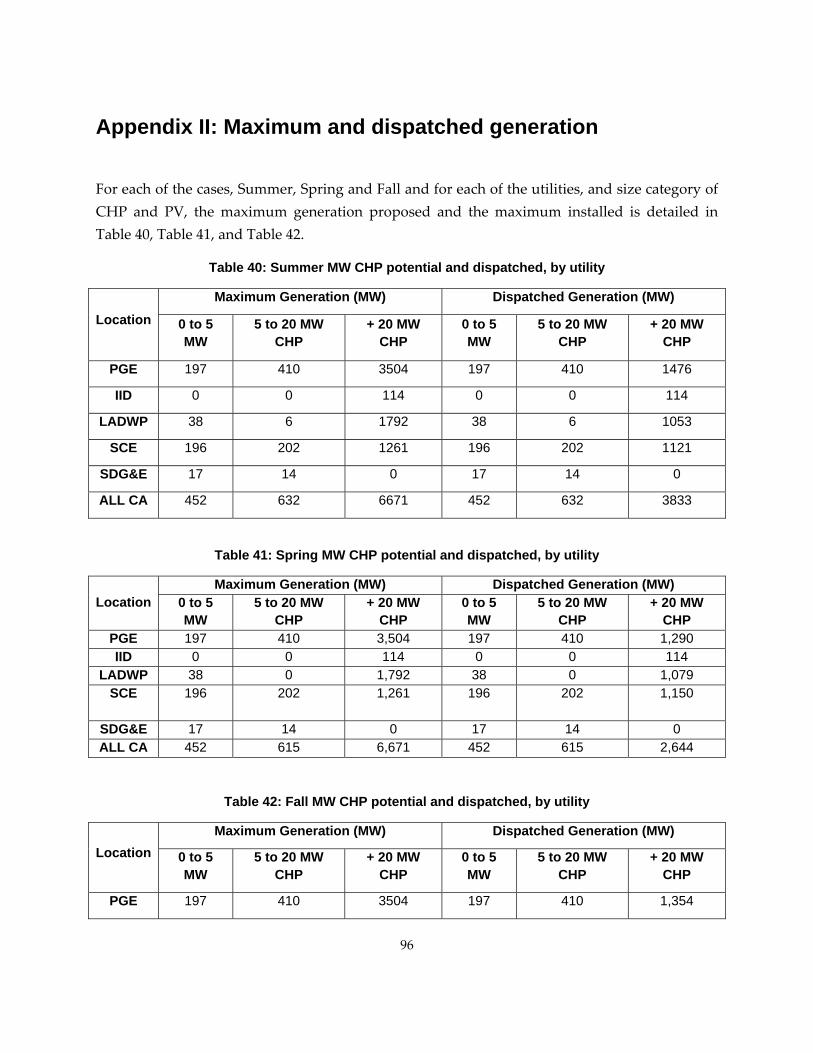
Appendix II: Maximum and dispatched generation

96

For each o egory of CHP  a u tion  pro aximum iled  in Table 40,   Table 42.   

Table 40: Summer MW CHP po atched, by utility

Location Maximum Generation (MW) tched Gene (MW)

f the cases, Summer, Spring and Fall and for each of the utilities, and size catnd  PV,  the maxim m  genera posed  and  the m   installed  is  deta

Table 41, and

tential and disp

Dispa ration

0 to 5 MW

5 to 20 MW CHP

+ 20 MW CHP

to 5 5 to 20 MWCHP

+ 20 MW CHP MW

0

PGE 197 410 3504 410 1476 197

IID 0 0 114 0 114 0

LADWP 38 6 6 1053 1792 38

SCE 196 202 1261 202 1121 196

SDG&E 17 14 14 0 0 17

ALL CA 452 632 632 3833 6671 52 4

Table 41: S W CHP pote atched, by utility

Location Maximum Generation (MW atched Generation (MW)

pring M ntial and disp

) Disp0 to 5 MW

5 to 20 MW CHP

+ 20 M 5 to 20 MWCHP

+ 20 MW CHP

W 0 to 5CHP W M

PGE 197 410 410 1,290 3,504 197 IID 0 0 11 0 114 4 0

LADWP 38 0 1,792 0 1,079 38SCE 196 202 1,261 6 202 1,150 19

SDG&E 17 14 14 0 0 17 ALL CA 452 615 6,671 615 2,644 452 

Table 42: Fall MW CHP pote hed, by utility

Location Maximum Generation (MW) atched Gene (MW)

nti atcal and disp

Disp ration

0 to 5 MW

5 to 20 M CHP

+ 20 MCHP

5 to 20 MWCHP

+ 20 MW CHP

W W 0 to 5 MW

PGE 197 410 410 1,354 3504 197

97

IID 0 0 114 0 0 70

LADWP 38 6 6 943 1,792 38

SCE 196 202 1,2 202 1,125 61 196

SDG&E 17 14 0 14 0 17

ALL CA 452 626 626 3,523 6,671 452

98

Appendix III: CHP Organized by type o and CHP si egory  

Table 43: Potential MW, split by type of in HP size category and Utility

f industry, utility ze cat

dustry, C

CHP CATEGORY UTILITY INDUSTRY TYPE MW POTENTIAL 0 TO 5 MW

LADWP CH S EMICAL 3.12 ELECTRONIC 3.51

FAB AL RICATED METPRODUCTS 6.18

FOOD 9.06 PETROLEUM 4.29

PRINTING 2.44 TEXTILES 2.97

IID CALS 0.88 CHEMIELECTRONIC 4.17

FABRICATED METAL 1.91 PRODUCTS

INSTRUMENTS 0.85 MISC. MANUFACTURE 0.68

PAPER 1.61 PRIMARY METAL IND 1.08 TRANSPORTATION 0.96

PG&E CALS 24.34 CHEMIELECTRONIC 1.98

FABRICATED METAL PRODUCTS 5.59

FOOD 81.03 INDUSTRIAL MACHINERY 0.78

INSTRUMENTS 1.11 LEATHER 1.46 LUMBER 21.71 PAPER 26.13

PETROLEUM 4.40 PRIMARY METAL IND 5.40

PRINTING 0.89 RUBBER 8.21

STONE & GLASS 4.49 TEXTILE 2.08

TRANSPORTATION 2.26 SCE APPAREL 0.60

CHEMICALS 8.67 ELECTRONIC 7.12

FABRICATED METAL PRODUCTS 9.36

99

FOOD 44.86 SCE FURNITURE 1.20

INDUSTRIAL MACHINERY 2.17 INSTRUMENTS 2.03

PAPER 28.67 PETROLEUM 4.90

PRIMARY METAL IND 2.81 RUBBER 9.87

STONE & GLASS 5.16 TEXTILE 2.40

TRANSPORTATION 7.45 SDG&E CHEMICALS 1.09

ELECTRONIC 3.21 FABRICATED METAL

PRODUCTS 0.87 FOOD 0.94

INDUSTRIAL MACHINERY 1.34 INSTRUMENTS 2.64

RUBBER 1.68 TRANSPORTATION 0.73

5 TO 20 MW IID FOOD 6.95

PG&E CHEMICALS 12.66 FOOD 151.39

FURNITURE 4.67 LUMBER 34.70 PAPER 33.57

PRINTING 12.10 RUBBER 6.41

STONE & GLASS 4.72 TRANSPORTATION 23.23

SCE CHEMICALS 37.72 FABRICATED METAL

PRODUCTS 6.34 FOOD 16.55

FURNITURE 4.53 INSTRUMENTS 10.40

PAPER 62.69 PETROLEUM 36.04

PRIMARY METAL IND 21.52 RUBBER 11.56

STONE & GLASS 4.60 TEXTILE 19.49

TRANSPORTATION 6.15 PAPER 5.71

>20 MW LADWP PETROLEUM 723.82

100

FOOD 45.88 TRANSPORTATION 25.62

IID FOOD 106.14 PG&E PETROLEUM 1931.80

PAPER 274.47 LUMBER 354.12

PRIMARY METAL IND. 35.44 SCE CHEMICALS 154.56

FOOD 140.50 PAPER 33.83

PETROLEUM 767.46 TRANSPORTATION 126.26