Geographic Constraints on Knowledge Spillovers: Political Borders vs. Spatial Proximity

The Geographic Scope of Knowledge Spillovers: Spatial Proximity, Political Borders and Non-Compete Enforcement

_______________

Jasjit SINGH Matt MARX 2011/44/ST (Revised version of 2010/03/ST)

The Geographic Scope of Knowledge Spillovers: Spatial Proximity, Political Borders and Non-Compete Enforcement Policy

Jasjit Singh*

Matt Marx**

Revisedversionof2010/03/ST

March 25, 2011

We thank INSEAD and the MIT Sloan School of Management for funding this research. We are grateful to Ajay Agrawal, James Costantini, Pushan Dutt, Lee Fleming, Josh Lerner, Ilian Mihov, Peter Thompson, Brian Silverman and Olav Sorenson, and we also thank seminar participants at INSEAD and conference participants at the Academy of Management 2010 Meetings and NUS 2010 Conference on Research in Innovation and Entrepreneurship for very helpful feedback. Any errors remain our own.

* Assistant Professor of Strategy at INSEAD, 1 Ayer Rajah Avenue, Singapore 138676 Ph: +65 6799 5341

Email: jasjit [email protected]

** Assistant Professor of Technological Innovation, Entrepreneurship, and Strategic Management at MIT Sloan School of Management, 50 Memorial Drive, E52-561 Cambridge, MA 02142, United States Ph: +1 617 253 5539 Email: [email protected]

A Working Paper is the author’s intellectual property. It is intended as a means to promote research to interested readers. Its content should not be copied or hosted on any server without written permission [email protected] Click here to access the INSEAD Working Paper collection

http://www.insead.edu/facultyresearch/research/search_papers.cfm

2

Abstract

Geographic localization of knowledge spillovers is a long-held tenet of economic geography.

However, empirical research has examined this phenomenon by considering only one geographic unit

(country, state or metropolitan area) at a time, and has not accounted for spatial distance in such

analyses. We accomplish both using a choice-based sampling framework to estimate the likelihood of

knowledge flow, as represented by a citation between random patents. In addition to a robust country

effect, we find a puzzling persistence of state-level localization that cannot be explained merely as an

outcome of spatial proximity. This effect is found to be more than just a manifestation of greater

mobility or closer networks within states, suggesting a role for state-level institutions. As a

demonstration that state-level policy could influence knowledge flow patterns, we find that a natural

experiment wherein Michigan inadvertently started enforcing non-compete agreements indeed led to a

decrease in localized spillovers in the state.

Keywords: Knowledge spillovers; Borders; Distance; Economic geography; Non-compete agreements; Patent Citations JEL classification: O30, O33, R10, R12

3

1. Introduction

Among the key tenets in the diffusion of knowledge is that technical spillovers are

geographically localized (Jaffe, Trajtenberg, and Henderson, 1993; Thompson and Fox-Kean, 2005).

Yet we still have only limited understanding of the exact geographic scope of these knowledge

spillovers. Although prior studies have examined localization for geographic units of varying scope

(country, state or metropolitan area) individually, few attempts have been made to consider these units

simultaneously in order to unpack the contribution of each. This leaves unresolved the issue of

whether localization effects demonstrated for one of the larger geographic units (country or state)

might merely be a manifestation of mechanisms that actually operate more locally (e.g., at the

metropolitan level). In addition, the exact spatial distance between the source and destination of

knowledge is rarely accounted for in previous models, raising a question about how much of the

observed country- or state-level effect really is attributable to mechanisms—such as institutional or

policy differences—truly related to the borders themselves as opposed to just resulting from spatial

distance not being considered in the empirical estimation.

Addressing the above gap in the literature is important, especially given the central role

assumptions surrounding the geographic scope of knowledge spillovers play in areas as diverse as

technological innovation, strategy, economic geography, international economics and

entrepreneurship. Our approach departs from previous studies in this tradition by making no ex ante

assumptions about the right geographic unit of analysis. Instead, we try to run a “horse race” among

different geographic variables to isolate the level at which localization mechanisms operate most

prominently. Specifically, we employ choice-based sampling logic to estimate a “citation function”

that models the likelihood of a knowledge flow, as manifested in citations between patents. This

regression approach allows us to simultaneously control for collocation of the source and destination

of knowledge within the same country, state or metropolitan area, and is refined further to also

account for fine-grained geographic distance. In doing so, we unbundle the extent to which observed

localization of knowledge flows is an outcome of (1) discrete impediments associated with one or

more geopolitical boundaries and/or (2) a decline in the intensity of knowledge flow with distance.

Consistent with previous studies, independent analyses we conducted at the national, state and

metropolitan levels exhibit strong evidence of localized knowledge diffusion at each level. The

coefficient estimates for variables of collocation at all three levels drop significantly when these are

4

included simultaneously in the regression model, showing as argued that only considering individual

units separately does overestimate their importance. Even with simultaneous consideration of the

three, however, the estimated country- and state-level effects do not disappear, demonstrating that the

original findings are not entirely driven by aggregation of more local (metropolitan-level) effects. We

next extend this analysis to include a full set of indicator variables that non-parametrically account for

effects of spatial distance. A majority of the national and state-level effects still persist, even though

there is also an independent effect of knowledge diffusion gradually decaying with distance. Finally,

as additional measures of geographic proximity, we introduce indicator variables to capture whether

the source and destination are in adjacent countries or states. While adjacency is indeed associated

with increased knowledge flow intensity, this effect is still significantly smaller than the effect of

collocation within the same country or state.

We investigate further to try to explain the robust border effects. Previous research has shown

that knowledge flow patterns are significantly affected by mobility of individuals and resulting

changes in interpersonal networks (Almeida and Kogut, 1999; Rosenkopf and Almeida, 2003; Song,

Almeida and Wu, 2003; Singh, 2005; Agrawal, Cockburn and McHale, 2006; Fleming, King and

Juda, 2007; Breschi and Lissoni, 2009; Singh and Agrawal, 2011). We therefore carry out further

analysis to examine whether the border effects persist even when variables capturing such “social

proximity” of knowledge source and destination are introduced. We capture the effect of inventor

mobility by including an indicator variable for an inventor being common between the teams of

inventors between which knowledge flows. We similarly account for interpersonal networks by

including indicator variables for direct or indirect collaborative ties between the source and

destination teams. Although we do find that these social proximity variables have strong effects of

their own, they have limited explanatory power as mediators: practically all of the country border

effect and most of the state border effect remains unexplained.

We view robust findings with regard to localization of knowledge flows associated with

national borders—even after controlling for other geographic dimensions—as not a big surprise, given

the well-documented linguistic, cultural, institutional and economic differences among countries (see,

e.g., Coe, Helpman and Hoffmaister, 2009). However, the persistence of a state border effect is more

puzzling, especially given the common perception that states are not a very relevant unit of analysis

for economic activity (Krugman, 1991; Breschi and Lissoni, 2001).

5

We carry out additional analysis to generate further insight into the state border effect.

Looking for possible time trends, we find the localization finding to not have decreased over time (at

least for our sample) despite the hype about globalization and the world becoming small. We find the

state effect to be particularly pronounced when individuals comprising the source and destination of

knowledge are not proximal in the collaborative network, are employees of different organizations, or

work in different technological domains. Contrary to expectations, the effect turns out to be stronger

for knowledge originating in non-firm entities (universities, research laboratories or government-

affiliated organizations) than it is for knowledge originating in firms.

In the last part of the paper, we consider the possibility that institutional factors that vary

across states might play a role in shaping knowledge diffusion patterns. Specifically, we investigate

whether a state-level policy variable—enforcement of employee non-compete agreements versus non-

enforcement—appears to have important consequences. In addition to cross-sectional evidence in line

with this conjecture, we also find that a natural experiment wherein Michigan inadvertently started

enforcing non-compete agreements also had an associated decrease (consistent with our prediction) in

localized knowledge spillovers in the state. Although this variable in itself does not explain all the

state-level knowledge spillover effect, it does suggest that looking for other institutional differences at

not just country but also state level might be fruitful for future research. This part of our analysis

contributes also to the growing literature on the various effects of non-compete covenants (Franco and

Mitchell, 2008; Marx, Strumsky and Fleming, 2009; Samila and Sorenson, 2011).

2. The Geographic Scope of Knowledge Spillovers

In examining the geographic scope of knowledge spillovers, a natural starting point for the

discussion is existing research studying localization (e.g., Jaffe, Trajtenberg and Henderson, 1993;

Almeida and Kogut, 1999; Thompson and Fox-Kean, 2005). This research has demonstrated the

phenomenon through separate analyses at different geographic levels, such as country, state and

metropolitan area. However, it provides limited guidance regarding the exact geographic scope of

knowledge spillovers. For example, although intra-country knowledge spillovers are found to be more

intense than those across countries (Branstetter, 2001; Keller, 2002; Singh, 2007), this might simply

reflect an aggregation of state- or metropolitan-level phenomena. Similarly, interpretation of state-

6

level localization findings (Jaffe, 1989; Audretsch and Feldman, 1996; Almeida and Kogut, 1999) is

unclear, since these might also be driven by effects actually operating at more local geographic levels.

These are therefore open to criticisms to the effect that “state boundaries are a very poor proxy for the

geographical units within which knowledge ought to circulate” (Breschi and Lissoni, 2001: 982).

Indeed, economic geographers have long argued that metropolitan boundaries are more appropriate as

the unit of analysis in examining such phenomena, echoing Krugman’s remark that “states aren’t

really the right geographic units” in economic analysis (Krugman, 1991:43).

The above ambiguities arise because localization effects have to date been investigated

through separate analyses examining knowledge flows at different geographic levels: the country, the

state and the metropolitan area. One could consider trying to figure out the relative importance of

different geographic levels by somehow comparing the findings across levels. However, given

limitations of existing methodology, this would likely be an incomplete and statistically inconclusive

exercise. What has probably prevented previous research from simultaneously considering multiple

geography-related measures is that the common approach (pioneered by Jaffe, Trajtenberg and

Henderson , 1993—henceforth referred to as JTH) used for examining the geography of knowledge

spillovers is not well-suited for the particular question we are interested in. Recognizing that

knowledge flows—measured using patent citations—might appear excessively localized in part due to

technological specialization of regions, the JTH approach statistically tests for localization of

knowledge spillovers by comparing the prevalence of collocation between the cited and citing patents

(representing the knowledge source and destination respectively) with that between the cited and

appropriate “control” patents selected through matching with the respective citing patents based on

their technological characteristics and temporal origin. With collocation within a certain geographic

region essentially being a dependent variable in this model, it is difficult to examine multiple

geographic levels at the same time. For our research question, we instead rely on a regression

framework that uses the likelihood of citation between two random patents as the dependent variable,

now being able to employ the entire set of geography-related variables as explanatory variables in the

same model.

In addition to not unpacking different geographic levels, existing research also does not

account for spatial distance, treating collocation within each geographic unit as just a measure for

geographic proximity itself without attempting to disentangle border and distance effects. Identifying

7

border effects truly associated with collocation within the same country or state, independent of

distance, would require a simultaneous consideration of borders and distance. Hardly any of the

studies have employed the fine-grained spatial data needed for this. Although a few have used at least

some distance-based measures, these have typically been too aggregate to disentangle all the

geographic effects of interest to us. For example, although Keller (2002) employs data on distance

between capital cities of countries, he does not consider different intra-country distances. Likewise,

Peri (2005) considers distances between different pairs of states, but does not distinguish different

city-to-city distances within a state. In this regard, there is a need to dig deeper into the geography of

knowledge spillovers in a manner analogous to a body of work in the literature on international trade,

which examines the role of geographic distance versus political borders at the country level (e.g.,

McCallum, 1995; Anderson and Wincoop, 2003) or state level (e.g., Wolf, 2000; Hillberry and

Hummels, 2003, 2008). This is what we attempt to do.

Our patent citation-level framework has the additional advantage of being flexible in

modeling technological relatedness between patents, allowing multiple levels of technological

granularity to be considered at the same time. This at least partly overcomes the challenge previous

studies have faced in having to choose a specific level of technological classification in

constructing the JTH-style control sample. As Thompson and Fox-Kean (2005) and Henderson,

Jaffe and Trajtenberg (2005) discuss, one faces a dilemma in using JTH-style matching: A three-

digit technology match (commonly employed) might be too crude to fully capture relevant

geographic distribution of technological activity, whereas a finer classification could suffer from a

selection bias because a stringent match would not be found for most of the sample. Both these

articles suggest that an appropriate regression approach might be a way out of this dilemma, a

suggestion we follow by implementing our citation-level model that also simultaneously accounts

for technological relatedness at multiple levels of granularity in estimating the likelihood of

citation between two patents.1 Before going into details of our regression framework, we discuss

how we constructed a dataset amenable to such an analysis.

1 For previous studies employing similar citation-level regression frameworks, see Sorenson and Fleming (2004) and Singh (2005). Although these studies also consider multiple technology-related variables, we consider a richer set of such variables. However, a bigger distinction between our approach and that of these previous studies is that, unlike these studies, we consider multiple geography-related explanatory variables at the same time.

8

3. Constructing the Dataset

Given the rich information they contain, patent data are particularly well-suited for examining

the questions of interest in this study. Information about citations between patents is readily available

as an indicator of knowledge flows. In addition, the ability to derive varied information regarding

geographic location of inventors—which we treat as the source and destination of knowledge flows—

is very useful.

While citation-based measures are noisy in capturing the underlying diffusion of knowledge,

direct surveys of inventors have established that citations—especially when employed in large

samples—do capture knowledge flows meaningfully (Jaffe and Trajtenberg, 2002; Duguet and

MacGarvie, 2005). Admittedly, there is disagreement regarding which citations to interpret as

knowledge flows. Considering citations added by patent examiners (rather than inventors themselves)

might or might not be desirable, depending on whether we believe an inventor was genuinely not

aware of a previous patent or (either mistakenly or strategically) just omitted the citations an examiner

subsequently added (Alcacer and Gittelman, 2006; Lampe, 2011). We consider all citations in our

measurement. While we would have liked to exclude examiner-added citations at least as a robustness

check, unavailability of machine-readable examiner citations for our sample period made this

impractical.

Admittedly, even assuming that citations do correctly capture knowledge flows, it is

impractical to decipher whether a given knowledge flow really represents a “spillover”—that is, a true

externality for which the receiver does not have to fully pay. Nevertheless, we follow the prevalent

view that studying knowledge flows is interesting nevertheless because they are likely to at least

partly represent spillovers and for the rest still represent benefits the receiver gets in the form of

“gains from trade” even when they reflect only market transactions rather than true externalities.

Our dataset combines raw data from the United States Patent and Trademark Office (USPTO)

with additional data from the National Bureau of Economic Research (NBER; see Jaffe and

Trajtenberg, 2002, Chapter 13) and the National University of Singapore-Melbourne Business School

patent database. As part of a multiyear research effort, this dataset has been further enhanced along

four dimensions. First, an elaborate inventor name-matching procedure has been carried out to map all

9

individual records to unique inventor identifiers.2 Second, for each assigned patent, information about

the parent organization has been further refined by carrying out an assignee name cleanup and a

subsequent parent-subsidiary match.3 Third, locations of U.S. inventors have been mapped to

“metropolitan areas” that reflect daily work-related commuting patterns of individuals within the

United States.4 Finally, city locations of inventors have been mapped to latitudes and longitudes on

the earth’s surface, allowing the use of spherical geometry in calculating the precise pair-wise

geographic distances.5

Our sample construction begins with a consideration of cited patents originating during the

period 1980 through 1986.6 Since we are interested in examining not just country border but also state

border effects, and consistent state identification information is available only for the United States,

we restrict the above sample to patents arising from inventors with U.S. addresses. Further, to be able

to cleanly identify different border and distance effects without having to make arbitrary assumptions

to resolve the locational ambiguity of a knowledge source, we restricted ourselves to patents whose

geographic origin is unambiguously defined. In other words, we exclude patents from geographically

dispersed inventor teams, even though these might be an interesting (but different) topic to study.

Finally, to allow computation of precise spatial distances between cities, we also drop the (relatively

infrequent) cases where a location cannot be mapped to a precise latitude and longitude. Together, the

2 We base our name-matching approach on Singh (2008), whose algorithms are similar to procedures

implemented by Trajtenberg (2006) and Fleming et al. (2007). 3 We have built upon the assignee matching procedure used by Singh (2005, 2007), who relies on NBER

Compustat identifiers, different corporate ownership directories and Internet sources. 4 The mapping relies on a concordance between U.S. cities and metropolitan areas from Thompson (2006).

These data include both MSAs and CMSAs, although for brevity we use the term MSA for both. Previous

studies sometimes define an additional “phantom MSA” per state to handle cases where a location does not fall

into an actual MSA. However, we do not because doing so effectively confounds intra-MSA effects with intra-

state effects. 5 This mapping, as described in Singh (2008), relies on the Geographic Names Information System of the U.S.

Geological Survey, Geonet Names Server of the National Geospatial Intelligence Agency and other sources. 6 We don’t sample beyond 1986 for two reasons. First, this leaves a long enough future time window to observe

diffusion of the underlying knowledge. Second, these patents are from a period prior to when the effect of a

policy change in Michigan (used as a natural experiment later in the paper) on the nature of patents could have

kicked in.

10

above steps lead to a final set of 116,975 potentially cited patents to be examined as potential sources

of knowledge.

For each patent, we determine the citations received during a 12-year window following the

application year. Following JTH, each original pair of patents involved in an actual citation is

matched to a “control pair” composed of the original cited patent and a “control patent” having the

same three-digit technology class and application year as the original citing patent. We then carry out

separate analyses to compare the extent of geographic collocation of the source and destination for the

original as well as control pairs, in turn using the country, the state and the metropolitan area as the

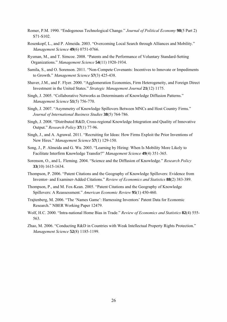
geographic units of analysis in the three different sets of calculations. As the side-by-side comparison

reported in Table 1 shows, our findings at each of the three units of analysis are quite comparable to

those reported in the pioneering JTH study as well as a more recent replication of the JTH results by

Thompson and Fox-Kean (2005). This should help assure the reader that our dataset is not in any way

particularly unusual.7

As mentioned earlier, the matching approach is not well-suited to directly addressing the two

questions central to our study: First, how much do national or state borders per se constrain

knowledge flow, as opposed to the observed effects at these levels being manifestations of

mechanisms that in fact operate at more local levels, such as metropolitan area? Second, do the

observed border effects truly represent a discrete change associated with the political borders

themselves rather than being a manifestation of an effect actually being driven by spatial proximity?

The right approach for answering these questions would be a regression framework that can

simultaneously examine the effect of different geographic boundaries while also directly considering

the role of geographic distance. The next section introduces such a framework.

7 While Thompson and Fox-Kean subsequently go on to make their matching approach more stringent by

employing nine-digit technology matching, they run into a challenge that over two-thirds of their patents cannot

be matched. Our approach is instead to stick to a three-digit initial match, but control for a finer technological

level through additional variables introduced directly into our regression model estimating the likelihood of a

patent citation.

11

4. A Citation-Level Regression Framework to Estimate Likelihood of Knowledge Flow

A seemingly straightforward (yet incorrect) extension of the JTH methodology might be to

employ a regression approach using a JTH-style matched sample in a (logit or probit) regression

model, wherein the existence of a citation between a pair of patents is taken as the dichotomous

dependent variable. However, this would imply that the JTH matching procedure is in effect used

to carry out sampling based on the dependent variable, since the JTH method draws a “zero”

(unrealized citation) corresponding to each “one” (actual citation). This needs to be somehow

corrected for in order to avoid biasing the estimates. Further, the potentially citing patents used in

constructing the control pairs are drawn (by the matching procedure) only from technology classes

and years from which citations to the potentially cited patent actually exist, ignoring the population

of potentially citing patents from the remaining technology classes and years. As the technical

appendix explains in detail, this can further bias the results. In this section, we describe a micro-

level citation regression framework that ameliorates these issues.

Before discussing how we extend our JTH-style matched sample to carry out patent-level

regression analysis, it is useful for exposition to first imagine a sample of patent pairs (to be

interpreted as either realized or unrealized citations) constructed by pairing each of our initial set

of potentially cited patents with a random draw of potentially citing patents. We could model the

likelihood of a patent citation in this sample as a Bernoulli outcome y that equals 1 with a

probability

ixii eβxxxy

1

1)()|1Pr(

Here, i is an index for the sample of potential citations (i.e., patent pairs), xi represents the vector

of covariates and controls (described later), and is the vector of parameters to be estimated.

Since the likelihood of a focal patent being cited by a random patent is extremely small, it

would not be practical to carry out the estimation based solely on the dataset constructed by using

random sampling from the population of all potentially citing patents. Instead, one might imagine

employing a “choice-based” sample, wherein the sampled fraction of potentially citing patents

that actually cite a focal patent is much larger than the fraction of the patents that are not

involved in a real citation to it. It is worth noting that a usual (unweighted) logistic estimation

12

based on such a sample would lead to biased estimates, since the sampling rate here is different for

different values of the dependent variable. One way to avoid the bias is to use the weighted

exogenous sampling maximum likelihood (WESML) approach, which involves a modified logistic

estimation based on first weighting each observation by the reciprocal of the ex ante probability of

its inclusion in the sample (Manski and Lerman, 1977).8

The basic WESML approach as described above is based on employing a sample where

the “zeroes” are drawn from the population of unrealized citations with the same ex ante

likelihood. Recognizing that technological relatedness is a particularly strong driver of citation

likelihood between patents, we can refine the choice-based sampling approach further to also get

benefits from stratification on this explanatory variable. This implies allowing the parameter to

vary across different y=0 subpopulations (Manski and McFadden, 1981; Amemiya, 1985, Ch. 9).

Indeed, by carefully considering the respective subpopulations (defined by different

technology classes and years of origin) from which we have effectively drawn our JTH-style

control patents in the previous section, we can interpret our matched sample as above and

appropriately calculate the weights to use with each control pair. However, as the technical

appendix explains in more detail, this is not sufficient in itself. Using the WESML approach with

the matched sample also requires extending the sample to ensure representation of potentially

citing patents belonging to years and/or technology classes not represented in the original patent

citations (and hence in the resulting matched sample). Doing so ensures that the strata considered

are not only mutually exclusive but also exhaustive in representing the full population of potential

citations. The above steps lead to our final sample of 2,779,345 patent pairs, which includes

709,279 actual citations (taking =1), 709,279 JTH-style matched pairs and 1,360,787 additional

pairs from citing classes and years not represented in the matched sample. An example included in

the technical appendix further illustrates the above sampling procedure as well as calculation of

appropriate weights for all the control observations.

Rather than making specific assumptions about the temporal pattern of citations, we

account for variation in citation likelihood with citation lag (i.e., years elapsed between the cited

8Please see the appendix for a more detailed description. For textbook treatment of choice-based sampling, see

Amemiya (1985, Ch. 9) or Greene (2003, Ch. 21). Sorenson and Fleming (2004) and Singh (2005) have

previously applied this approach in the context of patent citations.

13

and citing patents) non-parametrically—that is, by including among the covariates the full set of

indicator variables for different lags. We also include indicator variables for the cited patent’s

technological category and the citing patent’s year of origin to account for systematic differences

across sectors or over time.9 Finally, since the citation probability might also be driven by other

characteristics of the cited patent, we control for observable characteristics and employ clustering

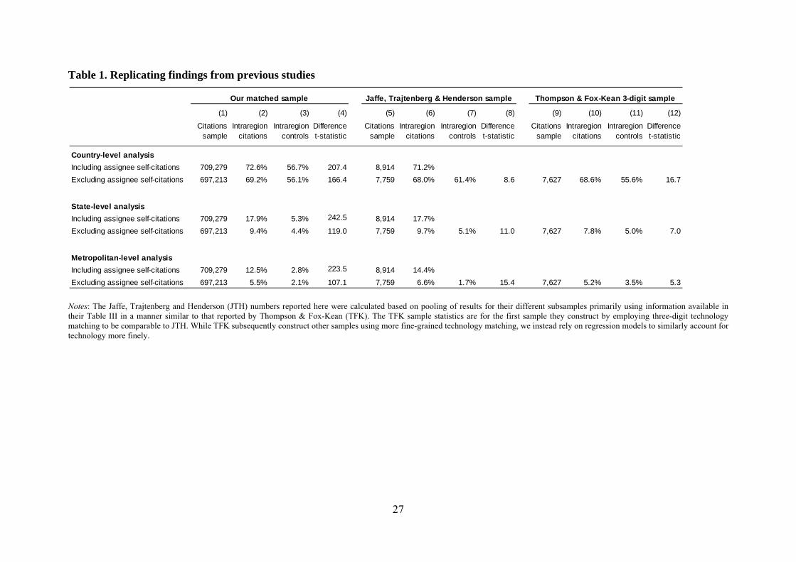
in the standard error computation to account for unobserved ones. Table 2 summarizes the key

variables used in our analyses.10

5. Results

5.1. Replicating findings from previous studies on localization of knowledge spillovers

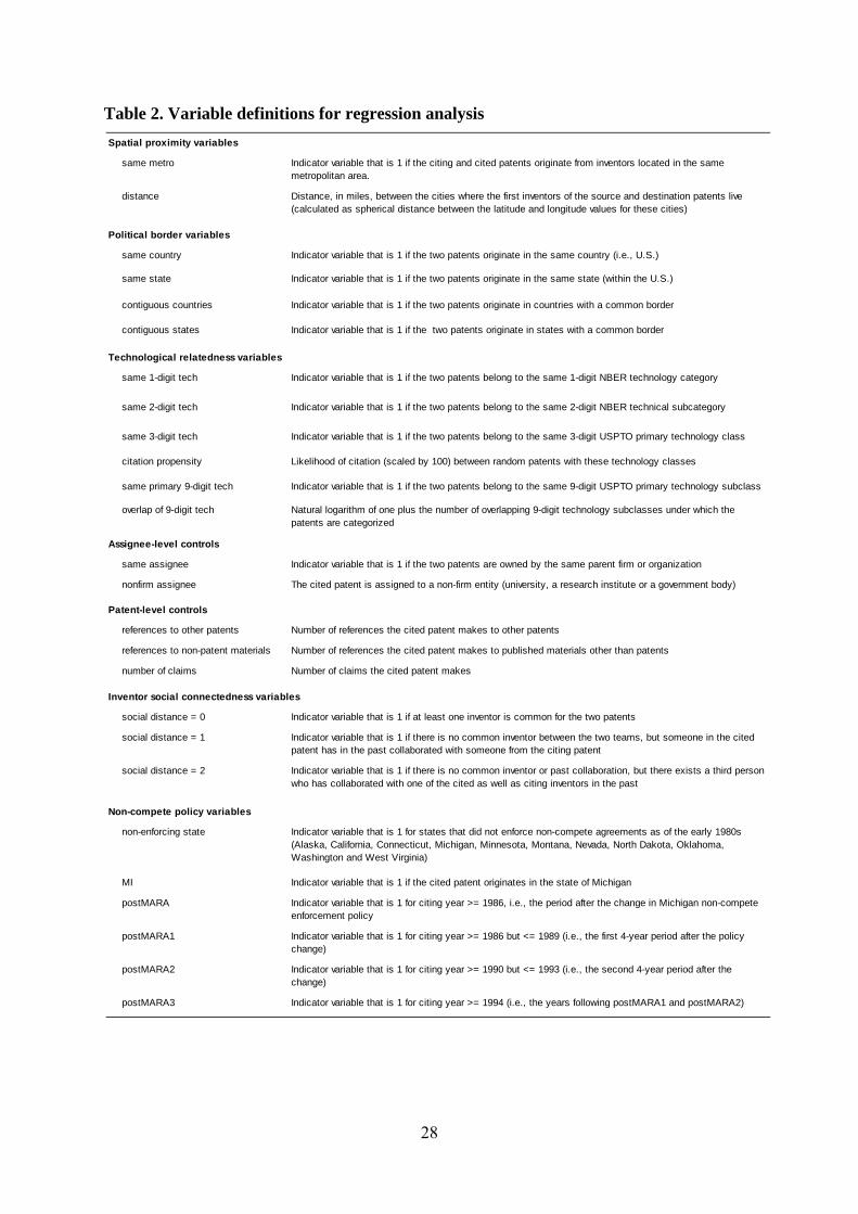
We begin by separately analyzing effects at the country, state and metropolitan levels;

results are reported in the first three columns of Table 3. For comparability with the JTH matching

approach, this initial analysis accounts for technological similarity and relatedness only up to the

three-digit technology classification, though our regression framework allows us to use a series of

indicator variables for this. As expected, we find knowledge flows within the same or related

technologies to be stronger than those across different technologies, as indicated by the positive

and significant estimates for same 1-digit tech, same 2-digit tech, same 3-digit tech and citation

propensity. Also, in line with intuition, within-assignee knowledge flows are stronger than those

across assignees, as indicated by the large positive estimate for same assignee.

More important, the findings are qualitatively consistent with localization effects detected

in findings from the conventional statistical tests reported in Table 1. We observe the localization

effect at all three geographic levels: the country (same country in column 1), the state (same state

9 Our goal here is simply to control for citation lag and citing year effects without trying to identify one of these

effects separately as in studies such as Rysman and Simcoe (2008). Given that perfect collinearity would result

if citation lag and citing year effects are included as the usual sets of indicators, we omit one of the indicator

variables. 10 The distance variables are not defined in the relatively infrequent cases (less than 7%) where either the cited

or the citing location could not be mapped to a precise latitude and longitude. To make sure that dropping these

in the distance-related regressions did not bias our findings in any way, we repeated the analysis by using the

average latitude and longitude for patents arising in the given state (for U.S. inventors) or country (for non-U.S.

inventors) to calculate approximate distance in such cases. Our key findings remained practically unchanged.

14

in column 2) and the metropolitan area (same metro in column 3). Additionally, the regression

estimates have an intuitive interpretation in terms of underlying relationships in the population:

they imply a 72% greater likelihood of within-country knowledge flow than that across national

borders, a 114% greater likelihood for within-state flow than that across state borders, and a 126%

greater likelihood for within-MSA flow than that across metropolitan boundaries.11 It might even

be tempting to compare these three numbers and conclude that the localization effects at the

metropolitan level are the strongest, at the state level they are a little less strong, and at the country

level localization is the weakest. However, such a comparison could be misleading because a

rigorous comparison among the effects operating at the three different geographic levels requires

simultaneous consideration of all three in a single regression model. We now turn to such analysis.

5.2. Simultaneously examining the role of geopolitical boundaries and spatial proximity

Simultaneously considering country-, state- and metropolitan-level effects, column 4 of

Table 3 finds the estimated independent effects for the three levels—same country (59%) and same

state (62%) and same metro (58%)—to be more comparable than what the above results might

suggest. Noting that the Thompson and Fox-Kean (2005) critique regarding the inadequacy of

three-digit technological controls still applies here, column 5 introduces additional control

variables to capture commonality of the nine-digit technology subclass (same primary 9-digit tech)

between the citing and cited patents as well as overlap along the secondary nine-digit technology

subclasses as well (overlap of 9-digit tech). Doing so raises the estimated effects slightly for the

national borders (63% now) and the state borders (65% now). However, the effect at the

metropolitan level (43% now) drops significantly. This appears in line with intuition, given that

geographic concentration of technological activity—which is what our technology-related control

11 In a logistic model, the marginal effect for a variable j is βj ’(xβ), which turns out to equal βj (xβ)[1-

(xβ)]. In general, this would need to be calculated based either on the mean predicted probability or using the

sample mean for (xβ). But the fact that citations are rare events allows further simplification: since (xβ) is

much smaller than 1, βj (xβ)[1-(xβ)] is practically equivalent to βj (xβ). This means the coefficient estimate

for βj can be directly interpreted as the percentage change in citation probability when the indicator variable j

goes from 0 to 1.

15

variables effectively control for—is naturally even greater when viewed at a finer level of

granularity for technology.

Considering multiple geographic units simultaneously indicates that there is more to the

national and state border effects than a mere aggregation of localization mechanisms operating at

the metropolitan level. We have however yet to rule out a possibility that such effects are not

epiphenomenal with spatial distance—that is, that merely including the metropolitan collocation

variable does not fully account for other distance-related effects that might be more gradual rather

than discretely associated with collocation within the same metropolitan area. This would require

making use of more fine-grained distance measures that can be constructed based on patent

records.

Accordingly, column 6 employs a series of indicator variables for different ranges of

distance to determine the extent to which greater within-region knowledge flow intensity could be

further explained simply by spatial proximity. The fine-grained distance indicators are mutually

exclusive, covering gradually increasing distances starting in the sequence distance = 0 miles (i.e.,

same city), distance >0 but <= 25 miles (i.e., not in the same city but still roughly within the same

metropolitan area) and so on. The omitted category in the regression model is instances with

distance greater than 4,000 miles.12 This non-parametric approach, based on a series of indicators

for distance without imposing any specific functional-form assumptions on how distance might

affect the likelihood of citation, ensures that the country- and state-level variables really do

measure the true border effects persisting once distance has been fully accounted for. (We also

tried even more fine-grained indicator variables, but that did not materially alter the findings.) Not

surprisingly, the estimates for the distance indicators themselves reveal that knowledge flows are

greatest when the source and the recipients are collocated within the same city and that the distance

effect gradually falls (more or less monotonically) with distance.13

12 In models not reported here, we instead tried just a same MSA variable distinct from two additional variables

for distance = 0 and distance > 0 miles but <= 25 miles. We found the same MSA variable to be insignificant,

i.e., to have no explanatory power beyond what distance captured directly. However, the same state and same

country effects still persisted as in the models reported here. 13 Carrying out an estimation of likelihood of citation as a function of a single distance variable—the logarithm

of spatial distance—leads to estimates implying a 23% fall in likelihood of citation with doubling of the

distance.

16

Comparing the estimated effects for country and state borders across columns 5 and 6, we

conclude that using fine-grained distance controls does significantly reduce these, with the

reduction being greater for the same state estimate than for the same country estimate. However,

the more important observation remains that the estimates for same country and same state are

both still quite large and robust. In contrast, when we include same metro in a regression otherwise

identical to model 6, the estimate for that practically disappears because metropolitan collocation is

now almost entirely accounted for by the distance = 0 miles and distance >0 but <=25 miles

indicator variables. This implies that, although distance completely explains the metropolitan

effect, the national and state border effects are to a large extent orthogonal to the effect of spatial

proximity per se. This conclusion challenges an interpretation that the localized knowledge

diffusion reported by previous studies is merely a manifestation of intra-regional distances being

on average smaller than cross-regional distances. Instead, factors such as institutional or cultural

mechanisms related to political borders might be playing an important role as well.

One might still wonder whether employing even fine-grained distance indicators might fail

to fully account for geographic proximity of countries or states within larger regions separated

from one another by natural barriers such as rivers, mountains, forests or deserts. We cannot fully

rule out the possibility of such non-distance geographic barriers, but as a robustness check the

model in column 7 employs two additional indicator variables—contiguous countries and

contiguous states—to distinguish cases where the source and destination are in different countries

or states but share a border. While we do find knowledge flow to be more intense between

contiguous regions than between non-contiguous regions, we find that independent country and

state border effects persist. (Note that the coefficients for same country and same state are not

directly comparable across columns 6 and 7 because introducing the variables for contiguity

changes the reference category.) The findings reported in subsequent tables also remain

qualitatively unchanged in similar checks involving including the contiguity variables.

5.3. Mediators and moderators for knowledge flow localization findings

To dig deeper into possible mechanisms driving the national and state border effects, Table

4 extends the above analysis to account for the social connectedness of inventor teams. (Column 1

reproduces results from column 6 of Table 3 for ease of comparison.) Motivated by the fact that

17

inventor mobility tends to be geographically localized, column 2 introduces a new indicator

variable: social distance = 0. It is defined in Table 2 as being 1 exactly in those cases where the

same inventor can be credited with both the citing and cited patent, and therefore covers cases of

inventor mobility across teams (which might or might not involve mobility across organizations,

which is already separately accounted for).14 While inventor mobility has a strong effect on patent

citation—in line with previous studies—it is found to have a more limited role as a mediator of the

knowledge flow effects documented above. Put differently, while an increase in knowledge flow

does seem to occur when mobility is involved (a conclusion subject to methodological caveats

discussed by Singh and Agrawal, 2011), mobility instances do not explain a large fraction of the

overall knowledge flow effect, possibly because such instances are relatively infrequent compared

with other factors.15

Recognizing that direct and indirect collaborative ties across individuals—which can also

facilitate knowledge flow—tend to be geographically proximate as well, column 3 introduces two

additional indicator variables that capture instances of inventors in the cited and citing team being

at social distance = 1 (defined in Table 2 as the case of former direct collaborators wherein

someone in the destination team has in the past collaborated with someone in the original team) or

at social distance = 2 (i.e., indirect collaborators wherein the teams are connected through a

common third person with whom someone from each team has previously collaborated). The

estimate for the country border effect remains practically unchanged relative to column 2, though

the state border effect does become smaller—albeit only by a small magnitude.

Moving beyond mediation, we try to generate more insight into the border effects by

looking at potential moderators for the effect of collocation within the same country or same state

on knowledge flow. We start by looking for a moderator role for the network variables already

considered above. The findings reported in column 4 reveal that network connectedness helps

reduce the constraints imposed by state but not country borders, with the localization effect within

a state being particularly prominent in its absence.

14 Note that here we are talking about self-citation by an inventor, which is distinct from accounting for self-

citation by an organization, which we already control for with the variable same assignee. 15 This could admittedly be driven, at least in part, by an inherent under-measurement of mobility when

employing patent data: we observe mobility only in cases where an inventor successfully files patents both pre-

and post-move. Therefore, we might be underestimating the role of mobility as a mediator for knowledge flow.

18

One might wonder whether the persistent localization effects we are picking up are driven

by observations from earlier in our sample (citing patents from the 1980s), and whether these

effects have subsequently fallen (for citing patents from the 1990s) with increased globalization

and continued advances in communication technologies. The analysis in column 5, which

examines time period as a moderator, finds no such decline in localization of knowledge flows

over time; in fact, the effect increases over time.

Columns 6, 7 and 8 explore other possible moderators. The results from column 6 show

knowledge flow being more localized within a state for across-technology knowledge flow than for

within-technology knowledge flow. A similar effect holds at the country level but is much weaker.

The findings in column 7 suggest that state borders constrain across-organization flows more than

within-organization flows. The result, surprisingly, reverses for country borders. The column 8

results suggest a pattern wherein localization of knowledge flows within states, though not so

much for those within countries, is stronger for patents arising from assignees other than firms,

such as universities, research laboratories or government organizations.

Overall, spillover localization evident at the country level might be unsurprising given the

well-documented linguistic, cultural, administrative and economic differences between countries

(see, e.g., Coe, Helpman and Hoffmaister, 2009). The persistence of a localization effect at the

state level—despite controls for geographic, social and technical distance—is more puzzling. The

finding raises a possibility that even institutional practices that vary at the state level might have a

role in shaping knowledge spillover patterns. We investigate one such factor in the next section.

5.4. Exploiting the role of non-compete enforcement policy

In the United States, individual states regulate many aspects of employment law, including

the use of employee non-compete covenants (hereafter, “non-competes”). These prevent former

employees from taking jobs at close competitors for a period of time, typically one to two years.

Non-competes are designed to stem the leakage of trade secrets, but they can also throttle the inter-

organizational mobility of workers within an industry (Fallick, Fleischman and Rebitzer 2007;

Marx, Strumsky and Fleming 2009; Garmaise, 2010; Marx, 2010). Accordingly, we would expect

fewer localized knowledge spillovers in states where non-competes are enforceable. The analysis

19

reported in column 9 of Table 4 carries out a cross-sectional comparison to test whether states that

enforce such agreements indeed exhibit less intrastate knowledge diffusion. As shown by the

coefficient on the interaction of same state and non-enforcing state (we use the term “non-

enforcing” to refer to states that do not enforce non-compete covenants), this does indeed appear to

be the case. These findings are, however, open to the obvious criticism that such an analysis also

needs to account for differences among states on myriad dimensions. Rather than attempting to do

so, we recognize that a cross-sectional comparison of states would inherently suffer from a concern

about unobserved heterogeneity. We therefore turn to a difference-in-differences analysis based on

an inadvertent non-compete policy change in the state of Michigan.

The natural experiment we exploit here has been previously documented and explained in

detail by Marx, Strumsky and Fleming (2009), so we provide only a brief description here.

Michigan prohibited the use of non-competes until 1985, when the Michigan Antitrust Reform Act

(MARA) was passed. MARA led to the repeal of numerous laws and acts including Public Act No.

329, which addressed antitrust provisions but also contained a prohibition on non-competes.

Lawmakers were apparently unaware that by passing MARA, they had lifted the long-standing ban

on non-competes. The legal community was not aware of the potential for the law to be reversed

but learned of the reversal quickly, making the MARA policy reversal an unanticipated and

exogenous event that provides the opportunity for a natural experiment as far as the change in non-

compete enforcement policy is concerned. Moreover, interviews with lawyers active at the time

indicate that the policy reversal was inadvertent and not subsequently repealed.

The heterogeneity in non-compete enforcement among U.S. states, coupled with Michigan’s

inadvertent reversal, facilitates a difference-in-differences analysis of knowledge flows originating in

Michigan versus other non-enforcing states in the pre-MARA versus post-MARA periods. The set of

cited patents we draw on for this analysis is from our 1980–86 sample as before, which—given the

typical lags between the actual R&D activity and the filing of the patent—implies that we are

examining diffusion of knowledge resulting from R&D activities carried out in the pre-MARA period.

Thus, our analysis avoids confounding knowledge diffusion effects with effects from the nature of

knowledge being generated in Michigan shifting as a result of MARA.

As a step-by-step description of our difference-in-differences logic, columns 1 through 4 in

Table 5 implement analyses analogous to the one carried out earlier, but for four different subsamples:

20

columns 1 and 2 consider citations made to Michigan patents in the pre-MARA and post-MARA

periods respectively, while those in columns 3 and 4 consider citations made to patents arising in

other non-enforcing states for the same periods. Of particular interest is that the same state coefficient

falls significantly for Michigan from column 1 to column 2, even as it actually increases for the other

non-enforcing states. In other words, relative to other non-enforcing states, Michigan appears to have

seen a decline in within-state knowledge flow after it started enforcing non-competes.

Column 5 pools the subsamples from the first four columns in order to replicate the

difference-in-differences analysis above in a single regression model, allowing more stringent

statistical testing. This requires additional variables (formally defined in Table 2) to be included in the

model. Consistent with our central finding from columns 1 through 4, the three-way interaction

among the variables MI, postMARA and same state is now found to be negative and significant. This

again implies that within-state localization of knowledge flows for Michigan fell significantly post-

MARA, relative to the trends one would expect in the knowledge flow patterns by looking at how

knowledge flows evolved for other non-enforcing states. The more detailed timing-related analysis in

column 6 reinforces the above findings, demonstrating that there is a significant drop in knowledge

flows for all three periods we split the post-MARA period into (1986–1989, 1990–1993 and post-

1993, as per the variable definitions summarized in Table 2). This seems in line with our expectation

that the effect would be roughly comparable in magnitude across the three periods.

To further ensure the comparability of Michigan and non-Michigan samples of cited patents,

columns 7 and 8 repeat the analysis for a subset wherein the cited patents from Michigan have been

matched one-to-one on technology class and year of origin with the cited patents from other non-

enforcing states included in the analysis. The main findings remain the same despite the sample now

being substantially smaller, comprising 5,796 of the 6,913 cited patents from Michigan in our original

sample that get matched to 5,796 cited patents from other non-enforcing states. Finally, columns 9

and 10 further examine the robustness of this result by using the entire sample—including patents

originating even from states that enforce non-competes—in the analysis. The key qualitative findings

remain essentially unchanged.

21

6. Discussion, Caveats and Conclusion

We start this section by summarizing the contribution this study makes to the literature on the

geography of knowledge spillovers. We use a regression framework based on choice-based sampling

to estimate the likelihood of knowledge flow, allowing us to simultaneously consider the impact of

different geopolitical units and disentangle “border effects” from “distance effects.” This represents a

significant advance over previous research, which has relied on separate analyses at the country, state

or metropolitan level and has interpreted geopolitical boundaries only as a proxy for distance rather

than disentangling related border effects from distance effects.16 Our approach allows inference

regarding the extent to which previous findings reflect discrete effects truly associated with national

or state borders as opposed to simply being an aggregation of metropolitan-level effects and/or a

manifestation of a gradual (negative) relationship between knowledge diffusion and distance. In

similarly accounting for technological relatedness between the citing and cited patents at multiple

levels of granularity, our regression framework also avoids challenges that past matching-based

studies have faced in having to restrict to a single level of technological granularity.

Consistent with existing evidence on knowledge diffusion patterns, we find the knowledge

flow likelihood to be correlated with collocation, irrespective of whether collocation is defined as

being in the same country, the same state or the same metropolitan area. When we consider the three

geopolitical levels simultaneously in our framework, both country- and state-level effects remain

significant despite each having a smaller economic magnitude, reflecting that there is more to these

border effects than mere aggregation of metropolitan-level effects. Even after we non-parametrically

control for the exact spatial distance between the source and destination of knowledge, the two border

effects persist. Our conclusion therefore is that it would be incorrect to treat collocation within the

same country or state merely as a proxy for spatial proximity.

Our finding that national borders have a strong effect in their own right (i.e., even after

accounting for sub-national effects as well as fine-grained geographic distance) might not be too

16 The only exception we know of is a recent (unpublished) paper by Belenzon and Schankerman (2010), who

do attempt disentangling distance and state border effects. However, they examine the specific context of

knowledge generated in universities, and also do not adjust the typical JTH-style sampling and observation

weights like we do to ensure unbiased estimation of the relationship between citation likelihood and geographic

variables of interest.

22

surprising. The literature on international trade already suggests several border-related variables one

could consider for digging deeper, such as linguistic, cultural, political and economic differences

between countries. Indeed, in analysis not reported here, we found knowledge flows from the United

States to other English-speaking countries to be particularly strong even after accounting for the effect

of geographic distance. A more general treatment of variables use in gravity-type models from

international economics would, however, require a sample where not just the citing but also the cited

patents are drawn from multiple countries. Such an approach would not fit within the scope of the

present study, given our emphasis on simultaneously also accounting for state-level patterns of

knowledge diffusion—something we find practical only for knowledge originating in the United

States, since there is no readily available mapping of patents originating elsewhere in geographic units

analogous to U.S. states.

Our finding that even state borders matter in a way that is more than simply an aggregation of

metropolitan-level effects or even spatial proximity more broadly is more puzzling. We are unable to

explain this even by accounting for self-citation by organizations and social proximity of inventors.

This suggests that mechanisms fundamentally associated with not just country borders but also state

borders might play an important role in shaping knowledge diffusion patterns. If, contrary to

Krugman’s (1991) claim, states indeed are an interesting geographic unit at which to analyze

knowledge spillovers, further investigation seems warranted into state-level institutional or other

factors that could shape knowledge flow patterns. We take a first step in this direction by establishing

that the enforcement of employee non-compete agreements attenuates the diffusion of knowledge, an

effect we find both in cross-sectional comparison across states as well as in a difference-in-differences

analysis based on a natural experiment involving an inadvertent change in Michigan’s non-compete

enforcement policy in 1985. While these findings are interesting, this policy variable in itself does not

explain away the state-level localization effect. Future research should therefore continue to

investigate underlying mechanisms and institutional factors that might be shaping the geography of

knowledge diffusion.

While further exploration of state-level institutions and policies seems promising for future

research, we cannot rule out the possibility that at least some of the effects we find will turn out not to

be robust using more refined research designs in future work. Therefore, we view our study only as an

initial inquiry into border-related effects in knowledge diffusion. At a minimum, however, our

23

findings do call for further empirical investigation into disentangling different border versus distance

effects for flow of ideas, paralleling the trade literature in economics that investigates how real and

robust national and state border effects are in the context of flow of goods (McCallum, 1995; Wolf,

2000; Anderson and Wincoop, 2003; Hillberry and Hummels, 2003, 2008).

Thinking about managerial implications, we note that an agenda of developing a better

understanding of the geographic scope of spillovers is important from the point of view of firm

strategy. For example, in fully understanding the implications and trade-offs involved in opening a

knowledge-intensive subsidiary (e.g., an R&D lab) in a given location, a manager ought to consider

all geography-related aspects of the decision. While it is commonly emphasized that a firm benefits

from knowledge spillovers from other local players such as universities, research laboratories and

even competitors, we know relatively little about how much relative contribution collocating within

the same metropolitan area, the same state or the same country makes, and whether there is more to

this decision than what only spatial proximity considerations would suggest. Likewise, examining the

issue is of interest from the point of view of a firm concerned not about acquiring external knowledge

but about erosion of its uniqueness if its knowledge spills over to competitors (Kogut and Chang,

1991; Shaver and Flyer, 2000; Chung and Alcacer, 2002; Zhao, 2006; Alcacer and Chung, 2007).

Further progress toward unpacking the geography of knowledge spillovers would also help

refine existing theoretical models of innovation, entrepreneurship and growth, ultimately leading to

more effective innovation-related policies. For example, an assumption about intense knowledge

spillovers operating at the national level is central to many models of endogenous growth, which use

this to show how such constraints on access to foreign knowledge can limit a lagging country’s ability

to catch up (Romer, 1990; Grossman and Helpman, 1991). The extent to which knowledge spillovers

may be localized even at a subnational level, such as within states or even metropolitan areas, can

have important implications for policies geared toward encouraging local R&D or facilitating

knowledge diffusion (Peri, 2005). Finally, assumptions regarding the extent to which mechanisms

underlying knowledge diffusion operate at the metropolitan level are an important component of the

way economic geographers view the phenomenon of agglomeration of economic activity (Feldman

and Audretsch, 1999; Glaeser, 1999; Fallick, Fleischman and Rebitzer, 2006; Furman and MacGarvie,

2007). A better understanding of the role really played by each geographic variable should naturally

benefit policy makers in best leveraging the knowledge spillovers for regional growth.

24

References

Alcacer, J., and M. Gittelman. 2006. “Patent Citations as a Measure of Knowledge Flows: The Influence of Examiner Citations.” Review of Economics and Statistics 88(4) 774-779.

Alcacer, J., and W. Chung. 2007. “Location Strategies and Knowledge Spillovers.” Management Science 53(5) 760-776.

Agrawal, A., I. Cockburn and J. McHale. 2006. “Gone but Not Forgotten: Labor Flows, Knowledge Spillovers, and Enduring Social Capital.” Journal of Economic Geography 6(5) 571-591.

Almeida, P., and B. Kogut. 1999. “Localization of Knowledge and the Mobility of Engineers in Regional Networks.” Management Science 45(7) 905.

Amemiya, T. 1985. Advanced Econometrics. Cambridge, Mass.: Harvard University Press.

Anderson, J.E., and E.V. Wincoop. 2003. “Gravity with Gravitas: A Solution to the Border Puzzle.” American Economic Review 93 170-192.

Audretsch, D., and M. Feldman. 1996. “R&D Spillovers and the Geography of Innovation and Production.” American Economic Review 86(3) 630-640.

Belenzon, S., and M. Schankerman. 2010. “Spreading the Word: Geography, Policy and University Knowledge Diffusion.” Working Paper, Fuqua School of Business, Duke University.

Branstetter, L.G. 2001. “Are Knowledge Spillovers International or Intranational in Scope?” Journal of International Economics 53(1) 53-79.

Breschi, S., and F. Lissoni. 2001. “Knowledge Spillovers and Local Innovation Systems: A Critical Survey.” Industrial and Corporate Change 10(4) 975-1005.

Breschi, S., and F. Lissoni. 2009. “Mobility of Skilled Workers and Co-invention Networks: An Anatomy of Localized Knowledge Flows.” Journal of Economic Geography 9(4) 439-468.

Chung, W., and J. Alcacer. 2002. “Knowledge Seeking and Location Choice of Foreign Direct Investment in the United States.” Management Science 48(12) 1534-1554.

Coe, D.T., E. Helpman and A.W. Hoffmaister. 2009. “International R&D Spillovers and Institutions.” European Economic Review 53(7) 723-741

Duguet, E., and M. MacGarvie. 2005. “How Well Do Patent Citations Measure Knowledge Spillovers? Evidence from French Innovation Surveys.” Economics of Innovation and New Technology 14(5) 375-393.

Fallick, B., C. Fleischman and J. Rebitzer. 2006. “Job-Hopping in Silicon Valley: Some Evidence Concerning the Micro-Foundations of a High Technology Cluster.” Review of Economics and Statistics. 88(3) 472-481.

Feldman, M.P., and D.B. Audretsch. 1999. “Innovation in Cities: Science-based Diversity, Specialization and Localized Competition.” European Economic Review 43 409-429.

Fleming, L., C. King and A. Juda. 2007. “Small Worlds and Regional Innovation.” Organization Science 18(6) 938-954.

Franco, A.M., and M.F. Mitchell. 2008. “Covenants Not to Compete, Labor Mobility, and Industry Dynamics.” Journal of Economics and Management Strategy 17 581-606.

Furman, J.L., and M.J. MacGarvie. 2007. “Academic Science and the Birth of Industrial Research Laboratories in the U.S. Pharmaceutical Industry.” Journal of Economic Behavior & Organization 63 756-776.

25

Garmaise, M. 2010. “The Ties That Truly Bind: Noncompetition Agreements, Executive Compensation, and Firm Investment,” Journal of Law, Economics, and Organization, forthcoming.

Glaeser, E.L. 1999. “Learning in Cities.” Journal of Urban Economics 46(2) 254-277.

Greene, W.H. 2003. Econometric Analysis, 5th ed. Upper Saddle River, N.J.: Prentice Hall.

Grossman, G., and E. Helpman. 1991. Innovation and Growth in the World Economy. Cambridge, Mass.: MIT Press.

Henderson, R., A. Jaffe, and M. Trajtenberg. 2005. “Patent Citations and the Geography of Knowledge Spillovers: A Reassessment: Comment.” American Economic Review 95(1) 461-464.

Hillberry, R., and D. Hummels. 2003. “Intranational Home Bias: Some Explanations.” The Review of Economics and Statistics 85(4) 1089-1092.

Hillberry, R., and D. Hummels. 2008. “Trade Responses to Geographic Frictions: A Decomposition Using Micro-data.” European Economic Review 52(3) 527-550.

Imbens, G.W., and T. Lancaster. 1996. “Efficient Estimation and Stratified Sampling.” Journal of Econometrics 74 289-318.

Jaffe, A.B. 1989. “Real Effects of Academic Research.” American Economic Review 79(5) 957.

Jaffe, A.B., and M. Trajtenberg. 2002. Patents, Citations & Innovations: A Window on the Knowledge Economy. Cambridge, Mass.: MIT Press.

Jaffe, A.B., M. Trajtenberg and R. Henderson. 1993. “Geographic Localization of Knowledge Spillovers as Evidenced by Patent Citations.” Quarterly Journal of Economics 434 578-598.

Keller, W. 2002. “Geographic Localization of International Technology Diffusion.” American Economic Review 92(1) 120-142.

Kogut, B., and S.J. Chang. 1991. “Technological Capabilities and Japanese Foreign Direct Investment in the United States.” Review of Economics & Statistics 73(3) 401.

Krugman, P. 1991. Geography and Trade. Leuven, Belgium: Leuven University Press.

Lampe, R. 2011. Strategic Citation. The Review of Financial Studies, forthcoming.

Manski, C.F., and S.R. Lerman. 1977. “The Estimation of Choice Probabilities from Choice Based Samples.” Econometrica 45(8) 1977-88.

Manski, C.F., and D. MacFadden. 1981. “Alternative Estimators and Sample Designs for Discrete Choice Analysis.” In C. Manski and D. McFadden, eds., Structural analysis of discrete data with econometric applications. Cambridge, Mass.: MIT Press.

Marx, M., D. Strumsky and L. Fleming. 2009. “Mobility, Skills, and the Michigan Non-compete Experiment.” Management Science 55(6) 875-889.

Marx, M. 2010. “Good Work If You Can Get It…Again: Post-employment Restraints and the Inalienability of Expertise,” Working paper, MIT Sloan School of Management.

McCallum, J. 1995. “National Borders Matter: Canada-U.S. Regional Trade Patterns.” American Economic Review 85(3) 615-623.

Peri, G. 2005. “Determinants of Knowledge Flows and their Effect on Innovation.” Review of Economics and Statistics 87(2) 308-322.

26

Romer, P.M. 1990. “Endogenous Technological Change.” Journal of Political Economy 98(5 Part 2) S71-S102.

Rosenkopf, L., and P. Almeida. 2003. “Overcoming Local Search through Alliances and Mobility.” Management Science 49(6) 0751-0766.

Rysman, M., and T. Simcoe. 2008. “Patents and the Performance of Voluntary Standard-Setting Organizations.” Management Science 54(11) 1920-1934.

Samila, S., and O. Sorenson. 2011. “Non-Compete Covenants: Incentives to Innovate or Impediments to Growth.” Management Science 57(3) 425-438.

Shaver, J.M., and F. Flyer. 2000. “Agglomeration Economies, Firm Heterogeneity, and Foreign Direct Investment in the United States.” Strategic Management Journal 21(12) 1175.

Singh, J. 2005. “Collaborative Networks as Determinants of Knowledge Diffusion Patterns.” Management Science 51(5) 756-770.

Singh, J. 2007. “Asymmetry of Knowledge Spillovers Between MNCs and Host Country Firms.” Journal of International Business Studies 38(5) 764-786.

Singh, J. 2008. “Distributed R&D, Cross-regional Knowledge Integration and Quality of Innovative Output.” Research Policy 37(1) 77-96.

Singh, J., and A. Agrawal. 2011. “Recruiting for Ideas: How Firms Exploit the Prior Inventions of New Hires.” Management Science 57(1) 129-150.

Song, J., P. Almeida and G. Wu. 2003. “Learning by Hiring: When Is Mobility More Likely to Facilitate Interfirm Knowledge Transfer?” Management Science 49(4) 351-365.

Sorenson, O., and L. Fleming. 2004. “Science and the Diffusion of Knowledge.” Research Policy 33(10) 1615-1634.

Thompson, P. 2006. “Patent Citations and the Geography of Knowledge Spillovers: Evidence from Inventor- and Examiner-Added Citations.” Review of Economics and Statistics 88(2) 383-389.

Thompson, P., and M. Fox-Kean. 2005. “Patent Citations and the Geography of Knowledge Spillovers: A Reassessment.” American Economic Review 95(1) 450-460.

Trajtenberg, M. 2006. “The ‘Names Game’: Harnessing Inventors’ Patent Data for Economic Research.” NBER Working Paper 12479.

Wolf, H.C. 2000. “Intra-national Home Bias in Trade.” Review of Economics and Statistics 82(4) 555-563.

Zhao, M. 2006. “Conducting R&D in Countries with Weak Intellectual Property Rights Protection.” Management Science 52(8) 1185-1199.

27

Table 1. Replicating findings from previous studies

Notes: The Jaffe, Trajtenberg and Henderson (JTH) numbers reported here were calculated based on pooling of results for their different subsamples primarily using information available in their Table III in a manner similar to that reported by Thompson & Fox-Kean (TFK). The TFK sample statistics are for the first sample they construct by employing three-digit technology matching to be comparable to JTH. While TFK subsequently construct other samples using more fine-grained technology matching, we instead rely on regression models to similarly account for technology more finely.

(1) (2) (3) (4) (5) (6) (7) (8) (9) (10) (11) (12)

Citations sample

Intraregion citations

Intraregion controls

Differencet-statistic

Citations sample




Citations sample




Country-level analysisIncluding assignee self-citations 709,279 72.6% 56.7% 207.4 8,914 71.2%Excluding assignee self-citations 697,213 69.2% 56.1% 166.4 7,759 68.0% 61.4% 8.6 7,627 68.6% 55.6% 16.7

State-level analysisIncluding assignee self-citations 709,279 17.9% 5.3% 242.5 8,914 17.7%Excluding assignee self-citations 697,213 9.4% 4.4% 119.0 7,759 9.7% 5.1% 11.0 7,627 7.8% 5.0% 7.0

Metropolitan-level analysisIncluding assignee self-citations 709,279 12.5% 2.8% 223.5 8,914 14.4%Excluding assignee self-citations 697,213 5.5% 2.1% 107.1 7,759 6.6% 1.7% 15.4 7,627 5.2% 3.5% 5.3

Jaffe, Trajtenberg & Henderson sample Thompson & Fox-Kean 3-digit sampleOur matched sample

28

Table 2. Variable definitions for regression analysis

Spatial proximity variables

same metro Indicator variable that is 1 if the citing and cited patents originate from inventors located in the same metropolitan area.

distance Distance, in miles, between the cities where the first inventors of the source and destination patents live (calculated as spherical distance between the latitude and longitude values for these cities)

Political border variables

same country Indicator variable that is 1 if the two patents originate in the same country (i.e., U.S.)

same state Indicator variable that is 1 if the two patents originate in the same state (within the U.S.)

contiguous countries Indicator variable that is 1 if the two patents originate in countries with a common border

contiguous states Indicator variable that is 1 if the two patents originate in states with a common border

Technological relatedness variables

same 1-digit tech Indicator variable that is 1 if the two patents belong to the same 1-digit NBER technology category

same 2-digit tech Indicator variable that is 1 if the two patents belong to the same 2-digit NBER technical subcategory

same 3-digit tech Indicator variable that is 1 if the two patents belong to the same 3-digit USPTO primary technology class

citation propensity Likelihood of citation (scaled by 100) between random patents with these technology classes

same primary 9-digit tech Indicator variable that is 1 if the two patents belong to the same 9-digit USPTO primary technology subclass

overlap of 9-digit tech Natural logarithm of one plus the number of overlapping 9-digit technology subclasses under which the patents are categorized

Assignee-level controls

same assignee Indicator variable that is 1 if the two patents are owned by the same parent firm or organization

nonfirm assignee The cited patent is assigned to a non-firm entity (university, a research institute or a government body)

Patent-level controls

references to other patents Number of references the cited patent makes to other patents

references to non-patent materials Number of references the cited patent makes to published materials other than patents

number of claims Number of claims the cited patent makes

Inventor social connectedness variables

social distance = 0 Indicator variable that is 1 if at least one inventor is common for the two patents

social distance = 1 Indicator variable that is 1 if there is no common inventor between the two teams, but someone in the cited patent has in the past collaborated with someone from the citing patent

social distance = 2 Indicator variable that is 1 if there is no common inventor or past collaboration, but there exists a third person who has collaborated with one of the cited as well as citing inventors in the past

Non-compete policy variables

non-enforcing state Indicator variable that is 1 for states that did not enforce non-compete agreements as of the early 1980s (Alaska, California, Connecticut, Michigan, Minnesota, Montana, Nevada, North Dakota, Oklahoma, Washington and West Virginia)

MI Indicator variable that is 1 if the cited patent originates in the state of Michigan

postMARA Indicator variable that is 1 for citing year >= 1986, i.e., the period after the change in Michigan non-compete enforcement policy

postMARA1 Indicator variable that is 1 for citing year >= 1986 but <= 1989 (i.e., the first 4-year period after the policy change)

postMARA2 Indicator variable that is 1 for citing year >= 1990 but <= 1993 (i.e., the second 4-year period after the change)

postMARA3 Indicator variable that is 1 for citing year >= 1994 (i.e., the years following postMARA1 and postMARA2)

29

Table 3. Simultaneous consideration of political borders and spatial proximity in estimating likelihood of citation between two random patents

Notes: The unit of observation is pairs of patents representing actual or potential citations. The dependent variable is an indicator for whether or not the potentially citing patent actually cited the focal patent. A choice-based stratified sample is used, and a weighted logistic regression (WESML) approach is implemented using observation weights that reflect sampling frequency associated with different strata. The regression model also uses a constant term and indicator variables for citation lag, citing year and 1-digit NBER technology category, but these are not reported to conserved space. Robust standard errors are shown in parentheses, and are clustered on the cited patent. Asterisks indicate statistical significance (*** p<0.01, ** p<0.05, * p<0.1).

(1) (2) (3) (4) (5) (6) (7)

same country 0.716*** 0.593*** 0.632*** 0.408*** 0.510***(0.022) (0.016) (0.032) (0.037) (0.047)

same state 1.136*** 0.621*** 0.646*** 0.504*** 0.596***(0.044) (0.048) (0.067) (0.061) (0.077)

same metro 1.259*** 0.579*** 0.431***(0.064) (0.073) (0.130)

distance =0 miles (i.e., same city) 1.137*** 0.944**(0.369) (0.374)

distance >0 miles but <= 25 miles 0.817*** 0.621***(0.150) (0.160)


distance >50 miles but <= 75 miles 0.449*** 0.240**(0.101) (0.117)

distance >75 miles but <= 100 miles 0.444*** 0.250(0.169) (0.183)






distance >1000 miles but <= 2000 miles 0.250*** 0.142**(0.053) (0.062)


same 1-digit tech 1.047*** 1.051*** 1.049*** 1.052*** 1.048*** 1.048*** 1.048***(0.011) (0.011) (0.011) (0.011) (0.012) (0.012) (0.012)

same 2-digit tech 1.246*** 1.252*** 1.250*** 1.246*** 1.255*** 1.257*** 1.257***(0.014) (0.014) (0.014) (0.014) (0.016) (0.016) (0.016)

same 3-digit tech 2.774*** 2.724*** 2.736*** 2.724*** 2.327*** 2.322*** 2.320***(0.028) (0.028) (0.028) (0.027) (0.042) (0.039) (0.039)

citation propensity 3.883*** 3.886*** 3.898*** 3.960*** 2.757*** 2.817*** 2.817***(0.299) (0.298) (0.309) (0.280) (0.409) (0.371) (0.371)

same primary 9-digit tech 2.118*** 2.082*** 2.082***(0.132) (0.120) (0.120)

overlap of 9-digit tech 1.743*** 1.746*** 1.747***(0.039) (0.038) (0.038)

contiguous countries 0.142**(0.061)

contiguous states 0.356***(0.065)

same assignee 2.724*** 2.321*** 2.346*** 2.171*** 1.123*** 1.009*** 1.006***(0.068) (0.077) (0.080) (0.073) (0.145) (0.149) (0.149)

nonfirm assignee -0.074 -0.003 -0.010 -0.009 0.104*** 0.111*** 0.110***(0.049) (0.038) (0.041) (0.041) (0.036) (0.035) (0.035)

references to other patents 0.012*** 0.013*** 0.013*** 0.013*** 0.012*** 0.012*** 0.012***(0.001) (0.001) (0.001) (0.001) (0.002) (0.002) (0.002)

references to non-patent materials 0.073*** 0.062*** 0.059*** 0.068*** 0.024 0.023 0.023(0.021) (0.022) (0.022) (0.022) (0.039) (0.038) (0.038)

number of claims 0.010*** 0.009*** 0.009*** 0.009*** 0.008*** 0.008*** 0.008***(0.001) (0.001) (0.001) (0.001) (0.001) (0.001) (0.001)

Number of observations 2779345 2779345 2779345 2779345 2779345 2779345 2779345Wald chi2 198905 198529 201667 192776 157936 159841 160177Degrees of freedom 44 44 44 46 48 59 61

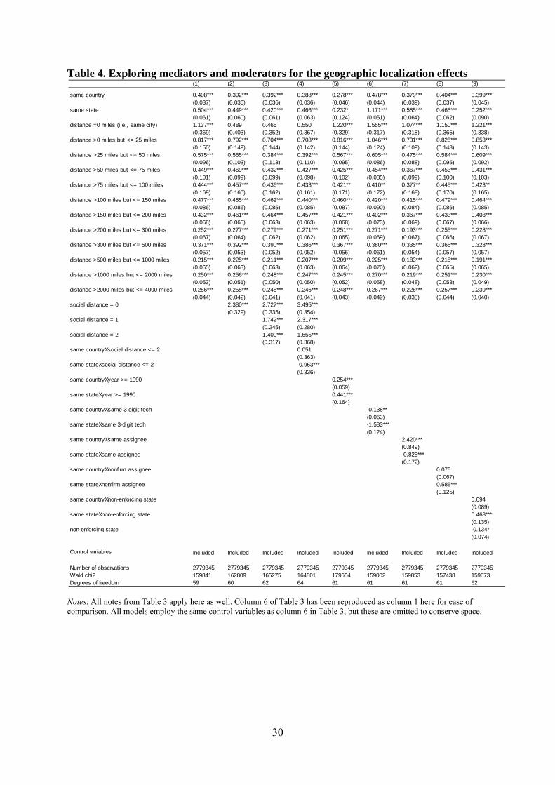
30

Table 4. Exploring mediators and moderators for the geographic localization effects

Notes: All notes from Table 3 apply here as well. Column 6 of Table 3 has been reproduced as column 1 here for ease of comparison. All models employ the same control variables as column 6 in Table 3, but these are omitted to conserve space.

(1) (2) (3) (4) (5) (6) (7) (8) (9)

same country 0.408*** 0.392*** 0.392*** 0.388*** 0.278*** 0.478*** 0.379*** 0.404*** 0.399***(0.037) (0.036) (0.036) (0.036) (0.046) (0.044) (0.039) (0.037) (0.045)

same state 0.504*** 0.449*** 0.420*** 0.466*** 0.232* 1.171*** 0.585*** 0.465*** 0.252***(0.061) (0.060) (0.061) (0.063) (0.124) (0.051) (0.064) (0.062) (0.090)

distance =0 miles (i.e., same city) 1.137*** 0.489 0.465 0.550 1.220*** 1.555*** 1.074*** 1.150*** 1.221***(0.369) (0.403) (0.352) (0.367) (0.329) (0.317) (0.318) (0.365) (0.338)

distance >0 miles but <= 25 miles 0.817*** 0.792*** 0.704*** 0.708*** 0.816*** 1.046*** 0.731*** 0.825*** 0.853***(0.150) (0.149) (0.144) (0.142) (0.144) (0.124) (0.109) (0.148) (0.143)



distance >75 miles but <= 100 miles 0.444*** 0.457*** 0.436*** 0.433*** 0.421** 0.410** 0.377** 0.445*** 0.423**(0.169) (0.160) (0.162) (0.161) (0.171) (0.172) (0.168) (0.170) (0.165)








social distance = 0 2.380*** 2.727*** 3.495***(0.329) (0.335) (0.354)

social distance = 1 1.742*** 2.317***(0.245) (0.280)

social distance = 2 1.400*** 1.655***(0.317) (0.368)

same countryXsocial distance <= 2 0.051(0.363)

same stateXsocial distance <= 2 -0.953***(0.336)

same countryXyear >= 1990 0.254***(0.059)

same stateXyear >= 1990 0.441***(0.164)

same countryXsame 3-digit tech -0.138**(0.063)

same stateXsame 3-digit tech -1.583***(0.124)

same countryXsame assignee 2.420***(0.849)

same stateXsame assignee -0.825***(0.172)

same countryXnonfirm assignee 0.075(0.067)

same stateXnonfirm assignee 0.585***(0.125)

same countryXnon-enforcing state 0.094(0.089)

same stateXnon-enforcing state 0.468***(0.135)

non-enforcing state -0.134*(0.074)

Control variables Included Included Included Included Included Included Included Included Included

Number of observations 2779345 2779345 2779345 2779345 2779345 2779345 2779345 2779345 2779345Wald chi2 159841 162809 165275 164801 179654 159002 159853 157438 159673Degrees of freedom 59 60 62 64 61 61 61 61 62

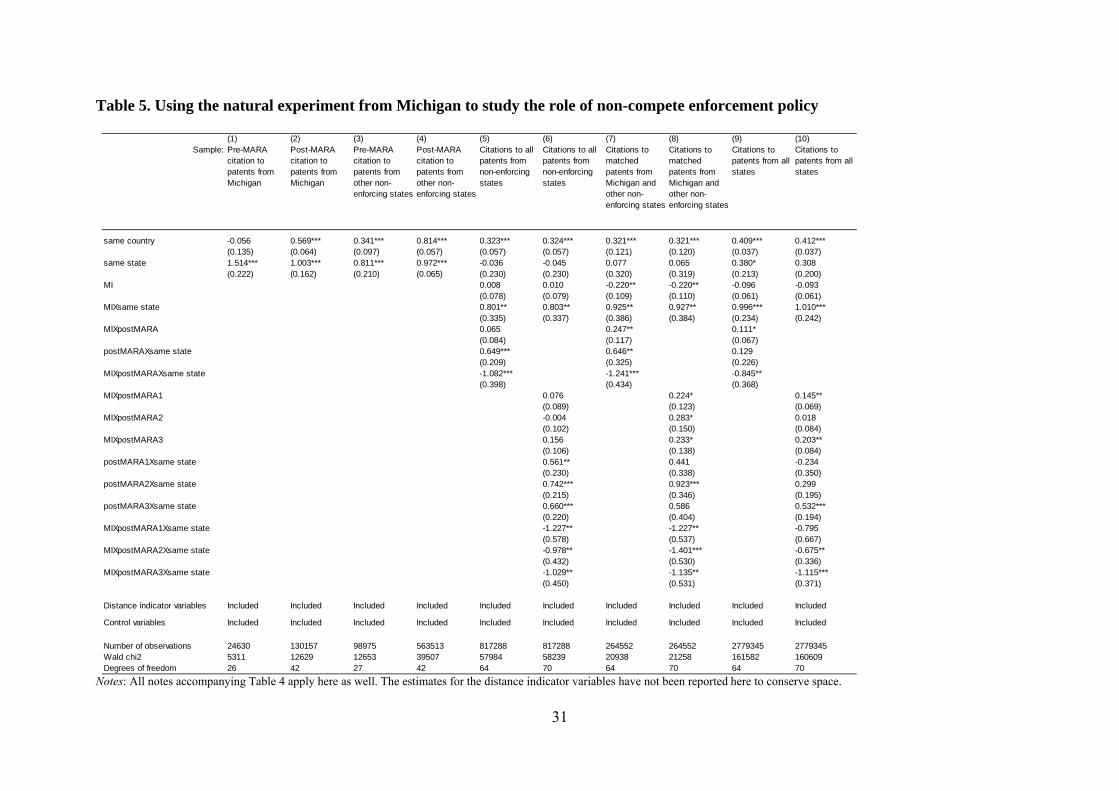
31

Table 5. Using the natural experiment from Michigan to study the role of non-compete enforcement policy

Notes: All notes accompanying Table 4 apply here as well. The estimates for the distance indicator variables have not been reported here to conserve space.

(1) (2) (3) (4) (5) (6) (7) (8) (9) (10)Sample: Pre-MARA

citation to patents from Michigan

Post-MARA citation to patents from Michigan

Pre-MARA citation to patents from other non-enforcing states

Post-MARA citation to patents from other non-enforcing states

Citations to all patents from non-enforcing states

Citations to all patents from non-enforcing states

Citations to matched patents from Michigan and other non-enforcing states

Citations to matched patents from Michigan and other non-enforcing states

Citations to patents from all states

Citations to patents from all states

same country -0.056 0.569*** 0.341*** 0.814*** 0.323*** 0.324*** 0.321*** 0.321*** 0.409*** 0.412***(0.135) (0.064) (0.097) (0.057) (0.057) (0.057) (0.121) (0.120) (0.037) (0.037)

same state 1.514*** 1.003*** 0.811*** 0.972*** -0.036 -0.045 0.077 0.065 0.380* 0.308(0.222) (0.162) (0.210) (0.065) (0.230) (0.230) (0.320) (0.319) (0.213) (0.200)

MI 0.008 0.010 -0.220** -0.220** -0.096 -0.093(0.078) (0.079) (0.109) (0.110) (0.061) (0.061)

MIXsame state 0.801** 0.803** 0.925** 0.927** 0.996*** 1.010***(0.335) (0.337) (0.386) (0.384) (0.234) (0.242)

MIXpostMARA 0.065 0.247** 0.111*(0.084) (0.117) (0.067)

postMARAXsame state 0.649*** 0.646** 0.129(0.209) (0.325) (0.226)

MIXpostMARAXsame state -1.082*** -1.241*** -0.845**(0.398) (0.434) (0.368)

MIXpostMARA1 0.076 0.224* 0.145**(0.089) (0.123) (0.069)

MIXpostMARA2 -0.004 0.283* 0.018(0.102) (0.150) (0.084)

MIXpostMARA3 0.156 0.233* 0.203**(0.106) (0.138) (0.084)

postMARA1Xsame state 0.561** 0.441 -0.234(0.230) (0.338) (0.350)

postMARA2Xsame state 0.742*** 0.923*** 0.299(0.215) (0.346) (0.195)

postMARA3Xsame state 0.660*** 0.586 0.532***(0.220) (0.404) (0.194)

MIXpostMARA1Xsame state -1.227** -1.227** -0.795(0.578) (0.537) (0.667)

MIXpostMARA2Xsame state -0.978** -1.401*** -0.675**(0.432) (0.530) (0.336)

MIXpostMARA3Xsame state -1.029** -1.135** -1.115***(0.450) (0.531) (0.371)

Distance indicator variables Included Included Included Included Included Included Included Included Included Included

Control variables Included Included Included Included Included Included Included Included Included Included

Number of observations 24630 130157 98975 563513 817288 817288 264552 264552 2779345 2779345Wald chi2 5311 12629 12653 39507 57984 58239 20938 21258 161582 160609Degrees of freedom 26 42 27 42 64 70 64 70 64 70

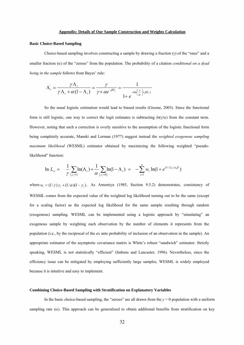
32

Appendix: Details of Our Sample Construction and Weights Calculation

Basic Choice-Based Sampling

Choice-based sampling involves constructing a sample by drawing a fraction () of the “ones” and a

smaller fraction () of the “zeroes” from the population. The probability of a citation conditional on a dyad

being in the sample follows from Bayes’ rule:

)(ln

'

1

1

)1( ii X

Xii

ii

ee

So the usual logistic estimation would lead to biased results (Greene, 2003). Since the functional

form is still logistic, one way to correct the logit estimates is subtracting ln(/) from the constant term.

However, noting that such a correction is overly sensitive to the assumption of the logistic functional form

being completely accurate, Manski and Lerman (1977) suggest instead the weighted exogenous sampling

maximum likelihood (WESML) estimator obtained by maximizing the following weighted “pseudo-

likelihood” function:

n

i

xyi

yi

yiw

ii

ii

ewL1

)21(

01

)1ln()1ln(1

)ln(1

ln

where )1)(/1()/1( iii yyw . As Amemiya (1985, Section 9.5.2) demonstrates, consistency of

WESML comes from the expected value of the weighted log likelihood turning out to be the same (except

for a scaling factor) as the expected log likelihood for the same sample resulting through random

(exogenous) sampling. WESML can be implemented using a logistic approach by “simulating” an

exogenous sample by weighting each observation by the number of elements it represents from the

population (i.e., by the reciprocal of the ex ante probability of inclusion of an observation in the sample). An

appropriate estimator of the asymptotic covariance matrix is White’s robust “sandwich” estimator. Strictly

speaking, WESML is not statistically “efficient” (Imbens and Lancaster, 1996). Nevertheless, since the

efficiency issue can be mitigated by employing sufficiently large samples, WESML is widely employed

because it is intuitive and easy to implement.

Combining Choice-Based Sampling with Stratification on Explanatory Variables

In the basic choice-based sampling, the “zeroes” are all drawn from the y = 0 population with a uniform

sampling rate (). This approach can be generalized to obtain additional benefits from stratification on key

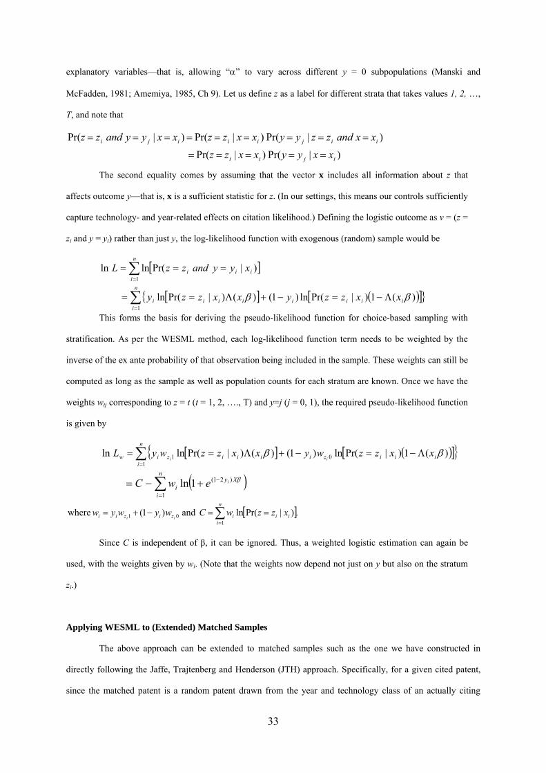
33

explanatory variables—that is, allowing “” to vary across different y = 0 subpopulations (Manski and

McFadden, 1981; Amemiya, 1985, Ch 9). Let us define z as a label for different strata that takes values 1, 2, …,

T, and note that

)|Pr()|Pr(

)|Pr()|Pr()|Pr(

ijii

iijiiiji

xxyyxxzz

xxandzzyyxxzzxxyyandzz

The second equality comes by assuming that the vector x includes all information about z that

affects outcome y—that is, x is a sufficient statistic for z. (In our settings, this means our controls sufficiently

capture technology- and year-related effects on citation likelihood.) Defining the logistic outcome as v = (z =

zi and y = yi) rather than just y, the log-likelihood function with exogenous (random) sample would be

n

iiii xyyandzzL

1

)|Pr(lnln

n

iiiiiiiii xxzzyxxzzy

1

)(1)|Pr(ln)1()()|Pr(ln

This forms the basis for deriving the pseudo-likelihood function for choice-based sampling with

stratification. As per the WESML method, each log-likelihood function term needs to be weighted by the

inverse of the ex ante probability of that observation being included in the sample. These weights can still be

computed as long as the sample as well as population counts for each stratum are known. Once we have the

weights wtj corresponding to z = t (t = 1, 2, …., T) and y=j (j = 0, 1), the required pseudo-likelihood function

is given by

n

i

Xyi

iewC1

)21(1ln

n

iiiizizii xzzwCwywyw

ii1

01 .)|Pr(ln and)1(where

Since C is independent of β, it can be ignored. Thus, a weighted logistic estimation can again be

used, with the weights given by wi. (Note that the weights now depend not just on y but also on the stratum

zi.)

Applying WESML to (Extended) Matched Samples

The above approach can be extended to matched samples such as the one we have constructed in

directly following the Jaffe, Trajtenberg and Henderson (JTH) approach. Specifically, for a given cited patent,

since the matched patent is a random patent drawn from the year and technology class of an actually citing

n

iiiiziiiiziw xxzzwyxxzzwyL

ii1

01 )(1)|Pr(ln)1()()|Pr(lnln

34

patent, we can interpret each {citing year, citing class} combination as a different stratum and calculate the

implied sampling rates based on the sample and population counts for each stratum to come up with appropriate

weights.

However, the matched sample in itself does not constitute a fully representative sample for the

population since the {citing year, citing class} combinations for which no actual citations (“ones”) exist are also

ignored from the point of view of the potential citations (“zeroes”). We need to ensure that the strata considered

are mutually exclusive and exhaustive in covering the entire population. To address this while still keeping the

number of strata manageable, we can create—for each cited patent—an additional observation for each citing

year by randomly selecting one potentially citing patent for each year (in the 12-year citing window) and

belonging to one of the technology classes from which no actual citation occurs to the focal cited patent (in that

year). The weight for each of these can again be computed using the implied sampling rates for random draws

from these subpopulations.

An example should help further clarify the sample construction. One of the patents in our set of cited

patents considered is patent number 4205881. This patent originated in application year 1980, and is classified

under the primary technology class 299. It receives two citations during the 12-year application time window of

1981–1992: from patent number 4441761 (year 1982, technology class 299) and patent number 4953915 (year

1989, class 299). Therefore patent pairs (4205881, 4441761) and (4205881, 4953915) become observations in

our dataset as actual citations (“ones”) with a weight of one each (since we include all citations, i.e., set = 1).

In JTH-based matching, citing patent 4441761 was matched to control patent 4402550 (year 1982,

class 299). In year 1982 and class 299, there were a total of 91 patents (excluding the citing patent itself), from

which patent 4402550 was chosen through a random draw. So the observation (4205881, 4402550) is included

in our dataset as a control pair (“zero”) with a weight of 91. Similarly, citing patent 4953915 mentioned above

was matched to control patent 4974907 (year 1989, class 299). In year 1989 and class 299, there were a total of

58 eligible patents, from which patent 4974907 was chosen through a random draw. So the observation

(4205881, 4974907) is included in our dataset as a control pair (“zero”) with a weight of 58.

Finally, for each of the years 1981 through 1992, we selected a random potentially citing patent,

constrained explicitly not to be from technology class 299 for the years 1982 and 1989 (as class 299 is already

included in finer strata above just for these two years). The range of weights for these 12 observations ended up

being between 61,000 and 104,000, depending on the number of eligible patents in the citing year being

considered for each.

Geographic Constraints on Knowledge Spillovers: Political Borders vs. Spatial Proximity

Documents