1 Introduction This paper introduces methods for the spatial analysis of social network data. Social network increasingly has a geographical component and it is possible spatially analyse sub-graph geographies. The paper describes methods for the identification of sub-graph regions that represent communities and mapping their spatial extent. It draws from research in statistical physics for partitioning networks in order to identify ‘communities’ or areas of the graph that are homogenous in some respect and from classic spatial analysis. In so doing it addresses recognised concerns over the reliability of the communities that are identified using these methods and the difficulty in understanding what they mean [1] [2]. 2 Social Network case studies Real networks tend to be irregular and highly heterogeneous, with specific parts of the network or graph (the terms are used interchangeably here) having high concentrations of interconnected vertices. The aim of community detection is to identify areas of the network that have high concentrations of edges that connect groups of vertices and that have low concentrations of edges between these groups. Such areas can be considered as ‘communities’ [3] Methods have been developed for partitioning networks in order to identify communities – areas within the graph (sub-graph areas) where the nature of interactions between vertices indicates some local clustering of interactions, under the assumption that sub- graph areas with high internal interactions are homogenous to some degree, depending on the nature of the network (social, publishing, cell phone etc). The interested reader is directed to number of reviews of the methods arising from statistical physics [1] [4] [5]. Recent work in the geography literature indicates that some community detection methods are more suitable for geographical applications than others because of the inviolable nature of topological network properties [6]. The case studies presented here identify methods for partitioning social network data into sub-graph areas and for examining their geographies. 3 Data Data was collected for an area of 30 km radius with its centre in Parliament Square in London. For each record (tweet), a number of items from the metadata of the message are returned including: • The username of the sender. • The content of the tweet. • The time the tweet was sent. • A geographical location the tweet was sent from. In the case studies specific tags in communications between social network data users (‘@user’ in Twitter data in this case) are used to identify and illustrate the connectedness of different concepts. The network is defined by the interactions (edges) between users (vertices). A subset of the data was analysed. It contained 87,555 records. Of these 52,397 contained tweets at (‘@’) a specific user, 52,280 that were not self tweets and 11,968 at users with a spatial reference (Geotag). At the end of the data cleaning, the network comprised 6,659 vertices and 7,491 edges (Figure 1). Thus only about 1% of the data contained an explicit spatial reference and were directed at another user. 4 Case Studies: analysis and results The case studies consider the identification of sub-graph areas from different perspectives: the identification of communities based on user to user interaction and mapping the probability surface associated with membership to that community. In both case studies the network constructed from geolocated @user tags are used to illustrate different approaches for identify communities in social network data. The analyses are sequential, building on the results of the previous example. The analyses uses functions available in the igraph package in R developed by Gábor Csárdi and Tamás Nepusz a description of which is available on the R website (http://cran.r-project.org/web/packages/igraph/igraph.pdf). The ‘igraph’ package offers a number of algorithms for visualisation. These generally involve find a set of locations in 2D space for the vertices that make the layout of edges easy to Geographic Analysis of Social Network Data Michael Batty, Andrew Hudson-Smith, Fabian Neuhaus & Steven Gray, University College London, UK, W1T 4TJ This research analyses social network data to identify communities or sub-graph regions. These sub-graph areas are indentified based on the arrangement of edges between vertices. The geographies of the communities are analysed, compared and visualised using kernel density estimations. A research agenda is suggested. Keywords: Graph Theory, Network Communities, Sub-Graph Geography, Twitter Data, London Abstract [email protected] [email protected] a.hudson-[email protected] [email protected] [email protected] [email protected].uk Chris Brunsdon University of Liverpool Liverpool, UK, L69 3BX Alexis Comber University of Leicester Leicester, UK, LE17 7RH Multidisciplinary Research on Geographical Information in Europe and Beyond Proceedings of the AGILE'2012 International Conference on Geographic Information Science, Avignon, April, 24-27, 2012 ISBN: 978-90-816960-0-5 Editors: Jérôme Gensel, Didier Josselin and Danny Vandenbroucke 293/392

Welcome message from author
This document is posted to help you gain knowledge. Please leave a comment to let me know what you think about it! Share it to your friends and learn new things together.
Transcript
1 Introduction
This paper introduces methods for the spatial analysis of social network data. Social network increasingly has a geographical component and it is possible spatially analyse sub-graph geographies. The paper describes methods for the identification of sub-graph regions that represent communities and mapping their spatial extent. It draws from research in statistical physics for partitioning networks in order to identify ‘communities’ or areas of the graph that are homogenous in some respect and from classic spatial analysis. In so doing it addresses recognised concerns over the reliability of the communities that are identified using these methods and the difficulty in understanding what they mean [1] [2].
2 Social Network case studies
Real networks tend to be irregular and highly heterogeneous, with specific parts of the network or graph (the terms are used interchangeably here) having high concentrations of interconnected vertices. The aim of community detection is to identify areas of the network that have high concentrations of edges that connect groups of vertices and that have low concentrations of edges between these groups. Such areas can be considered as ‘communities’ [3] Methods have been developed for partitioning networks in order to identify communities – areas within the graph (sub-graph areas) where the nature of interactions between vertices indicates some local clustering of interactions, under the assumption that sub-graph areas with high internal interactions are homogenous to some degree, depending on the nature of the network (social, publishing, cell phone etc). The interested reader is directed to number of reviews of the methods arising from statistical physics [1] [4] [5]. Recent work in the geography literature indicates that some community detection methods are more suitable for geographical applications than others because of the inviolable nature of topological network properties [6]. The case studies presented here identify methods for partitioning social network data into sub-graph areas and for examining their geographies.
3 Data
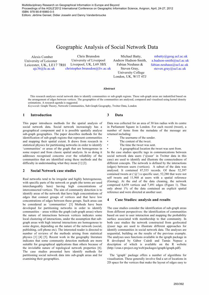
Data was collected for an area of 30 km radius with its centre in Parliament Square in London. For each record (tweet), a number of items from the metadata of the message are returned including: • The username of the sender. • The content of the tweet. • The time the tweet was sent. • A geographical location the tweet was sent from. In the case studies specific tags in communications between social network data users (‘@user’ in Twitter data in this case) are used to identify and illustrate the connectedness of different concepts. The network is defined by the interactions (edges) between users (vertices). A subset of the data was analysed. It contained 87,555 records. Of these 52,397 contained tweets at (‘@’) a specific user, 52,280 that were not self tweets and 11,968 at users with a spatial reference (Geotag). At the end of the data cleaning, the network comprised 6,659 vertices and 7,491 edges (Figure 1). Thus only about 1% of the data contained an explicit spatial reference and were directed at another user. 4 Case Studies: analysis and results
The case studies consider the identification of sub-graph areas from different perspectives: the identification of communities based on user to user interaction and mapping the probability surface associated with membership to that community. In both case studies the network constructed from geolocated @user tags are used to illustrate different approaches for identify communities in social network data. The analyses are sequential, building on the results of the previous example. The analyses uses functions available in the igraph package in R developed by Gábor Csárdi and Tamás Nepusz a description of which is available on the R website (http://cran.r-project.org/web/packages/igraph/igraph.pdf).
The ‘igraph’ package offers a number of algorithms for visualisation. These generally involve find a set of locations in 2D space for the vertices that make the layout of edges easy to
Geographic Analysis of Social Network Data Michael Batty,
Andrew Hudson-Smith, Fabian Neuhaus &
Steven Gray, University College
London, UK, W1T 4TJ
This research analyses social network data to identify communities or sub-graph regions. These sub-graph areas are indentified based on the arrangement of edges between vertices. The geographies of the communities are analysed, compared and visualised using kernel density estimations. A research agenda is suggested. Keywords: Graph Theory, Network Communities, Sub-Graph Geography, Twitter Data, London
Abstract
[email protected]@ucl.ac.uk
[email protected] [email protected]
Chris Brunsdon University of Liverpool
Liverpool, UK, L69 3BX
Alexis Comber University of Leicester Leicester, UK, LE17 7RH
Multidisciplinary Research on Geographical Information in Europe and Beyond Proceedings of the AGILE'2012 International Conference on Geographic Information Science, Avignon, April, 24-27, 2012 ISBN: 978-90-816960-0-5 Editors: Jérôme Gensel, Didier Josselin and Danny Vandenbroucke
293/392
AGILE 2012 – Avignon, April 24-27, 2012
see. Some graphs may be drawn in 2D space without any edges crossing (planar graphs) but this is not generally the case. However, choices of vertex layout that keep vertices joined by edges closer together generally lead to clearer visualisation. One approach to this is to use a vertex placement algorithm based on a model of the edges as a system of springs joined at the vertices, with edge weights being proportional to spring stiffness. The Fruchterman-Reingold algorithm is commonly used.
Figure 1. a) The network of users, displayed using a
Fruchterman-Reingold layout b) The network displayed over geographic space.
a)
b)
4.1 Community Detection
There are a number of methods arising from statistical physics, graph theory and network science for partitioning networks into communities. One of which is introduced and applied here. The basic premise in community detection algorithms is that areas in the network with higher than expected concentrations of edges connecting groups of vertices and with lower than expected concentrations of edges between these groups, can be considered as ‘communities’ [3]. Thus the properties of the network itself can be used to determine sub-graph areas.
This analysis used the Walktrap or Random Walk algorithm [7] to illustrate how networks can be partitioned into sub-graph areas. The Walktrap assumes that if a strong community exists within a network, then a random walker exploring the
network would spend a longer time ‘trapped’ inside any given sub-graph area. The algorithm defines a distance between vertices and between communities from the probabilities that the random walker moves from one vertex to another in a fixed number of steps. The number of steps has to be large enough to allow a significant portion of the network to be explored.
Modularity [8] provides a measure of the quality of any graph partition. It is one of the key concepts underpinning many community detection methods including Walktrap. Modularity is based on the fact that a random graph does not have communities within its structure and provides a measure of how unexpected the actual arrangements of edges between groups (sub-graph areas) is compared to a null model. Modularity Q for unweighted graphs is defined as:
!
Q =12m
(Aij " Pij )#(Ci,C j )$ (1)
where, A is the adjacency matrix, m the total number of edges of the graph, and Pij is the expected number of edges between vertices i and j in the null model [8]. The δ-function returns 1 if vertices i and j are in the same community (i.e. Ci = Cj), and zero otherwise. In the implementation of the Walktrap algorithm above, the optimal number of steps is that which returns the maximum modularity.
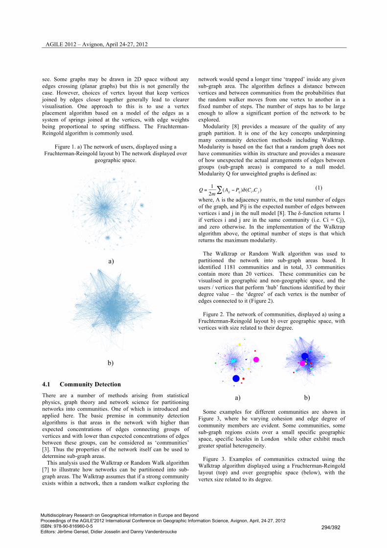
The Walktrap or Random Walk algorithm was used to partitioned the network into sub-graph areas based. It identified 1181 communities and in total, 33 communities contain more than 20 vertices. These communities can be visualised in geographic and non-geographic space, and the users / vertices that perform ‘hub’ functions identified by their degree value – the ‘degree’ of each vertex is the number of edges connected to it (Figure 2).
Figure 2. The network of communities, displayed a) using a
Fruchterman-Reingold layout b) over geographic space, with vertices with size related to their degree.
a) b)
Some examples for different communities are shown in
Figure 3, where he varying cohesion and edge degree of community members are evident. Some communities, some sub-graph regions exists over a small specific geographic space, specific locales in London while other exhibit much greater spatial heterogeneity.
Figure 3. Examples of communities extracted using the
Walktrap algorithm displayed using a Fruchterman-Reingold layout (top) and over geographic space (below), with the vertex size related to its degree.
Multidisciplinary Research on Geographical Information in Europe and Beyond Proceedings of the AGILE'2012 International Conference on Geographic Information Science, Avignon, April, 24-27, 2012 ISBN: 978-90-816960-0-5 Editors: Jérôme Gensel, Didier Josselin and Danny Vandenbroucke
294/392

AGILE 2012 – Avignon, April 24-27, 2012
Net
wor
k
Geo
grap
hy
a) Community 4 b) Community 11 c) Community 124
4.2 Mapping membership to particular communities
Kernel density estimation can be an exploratory tool for identifying hot-spots of activity related to a specific social network cluster. In this case study KDE methods are used to describe the spatial distribution of membership to individual communities. KDE identifies regions that have greater number of incidents than expected, analysed over cells in predefined grid. KDE models the relative density of the vertex locations (community members) as a surface created by summing the vertices in the sub-graph over a kernel function (a 2 dimensional distribution curve). Then for each cell, x, in a grid of discrete subdivisions of space, the relative likelihood of the occurrence of a vertex in that grid cell f(x) is computed in the following way:
!
f^(x) =
1nb
Kx " xib
#
$ %
&
' (
j=1
n
) (2)
where K() is a fixed kernel and b is the bandwidth defined by a multiple of the standard deviation of the kernel [8]. Kernel density estimators operate by averaging a small 'bump' (a probability distribution in 2D) centred on each observed point. The bandwidth of the kernel controls the smoothness of the estimate: very small values give rise to very 'spikey' surfaces, and large values to very flat ones. Thus typically they are chosen automatically, from the distribution of the points.
KDEs were generated for the communities described in the previous case study above and are illustrated in Figure 4a) to e). The surfaces reveal much more than simply locating the community member (vertex) locations as shown in Figure 3. The density surface value describe the intensity of the community’s presence in different locations. What it reveals is the very different spatial extent and density of each separate community. For example, Community 124 is medium in size with 208 users, but spatially concentrated in a specific area. By contrast, Community 4 is a much has 80 users but is much more widely distributed.
(1)
KDEs were generated for the communities described in the previous case study above and are illustrated in Figure 4a) to e). The surfaces reveal much more than simply locating the community member (vertex) locations as shown in Figure 3. The density surface value describe the intensity of the community’s presence in different locations. What it reveals is the very different spatial extent and density of each separate community. For example, Community 124 is medium in size with 208 users, but spatially concentrated in a specific area. By contrast, Community 4 is a much has 80 users but is much more widely distributed.
Figure 4. Kernel density surfaces showing the spatial extent
and spatial concentrations of different communities.
a) Community 4
b) Community 124
5 Discussion
This research has identified sub-graph communities within social network data based on tags and geo-location and has explored the geographical extent of communities. Methods from statistical physics used for partitioning networks were applied to social network data with explicit geographical attributes in order to analyse network structure. This allows the locality of communities within the global network of users to be identified. The geography could be identified location semantically from the tweets themselves (i.e. “I am going to Newcastle”). This is likely to be the most complex approach, although in principle it may be applied to any tweet. However,
Multidisciplinary Research on Geographical Information in Europe and Beyond Proceedings of the AGILE'2012 International Conference on Geographic Information Science, Avignon, April, 24-27, 2012 ISBN: 978-90-816960-0-5 Editors: Jérôme Gensel, Didier Josselin and Danny Vandenbroucke
295/392

AGILE 2012 – Avignon, April 24-27, 2012
a very large proportion of tweets will contain no information of this kind.
The geography of social networks is an increasingly important consideration in their analysis and study. A recent special issue of Social Networks (vol 34 issue 1) considered the spatial and social analysis of networks. Within this special issue papers examines co-offending ties and shows that co-offending is more likely between census tracts that are geographically closer [9]. Other work found that edges (ties) between social network vertices in different regional (geographical) communities were best predicted by the frequency of airline flights [10].
This paper has exemplified a number of methodological approaches and identified areas of further research, especially in relation to the geographic or locational aspects of social networks. These include:
• The need to examine different partitioning algorithms, especially as recent work has shown that there are not always appropriate for geographic applications [6].
• The formal investigation of different interpolation techniques to generate surfaces of community membership. These would the spatial distribution of the probability of any location being associated with any particular community at a given point in time
• Text mining analysis could be used to model the content of the interactions between users in a given community, identifying statistical topics associated with tweet content.
• Modularity is a measure of the quality of the network partitions and identifies statistically ‘surprising’ arrangements of edges. Alternative statistical and null should be investigated depending on the application / problem being .
• Methods for analysing semantics such as Latent Dirichlet Allocation or Probabilistic Latent Semantic Analysis could be also used to generate a weighted network based on the content of the network, which could then be analysed to identify partitions of areas of sub-graph homogeneity (communities).
• Examining the dynamics of network communities: how they change in spatial extent, membership and the content of their user interaction.
6 Conclusions
This research introduces statistical methods for analysing communities in social network data and their geographic extent. These that provide greater insight into social network structure, content, associated concepts and their geographical aspects. A research agenda is suggested as a result of these initial analyses.
References
[1] Porter, M.A., Onnela, J.-P. and Mucha, P.J., (2009). Communities in Networks. Notices of the AMS, 56(9): 1082-1166. [2] Newman, M.E.J., (2008). The physics of networks, Physics Today, 61(11): 33-38. [3] Girvan, M. and Newman, M.E.J., (2002). Community structure in social and biological networks. Proceedings of the National Academy of Sciences, 99: 7821-7826. [4] Fortunato, S., (2010). Community detection in graphs. Physics Reports, 486(3-5): 75-174. [5] Leicht, E.A. and Newman, M.E.J., (2008), Community structure in directed networks, Physical Review Letters, 100: 118703. [6] Comber A., Brunsdon, C. and Farmer, C. (in press). Community detection in spatial networks: inferring land use from a planar graph of land cover objects. Paper accepted for publication in International Journal of Applied Earth Observation and Geoinformation (January 2012) [8] Newman, M.E.J and Girvan, M., (2004). Finding and evaluating community structure in networks. Physical Review E, 69: 026113. [7] Pons, P. and Latapy, M., (2005). Computing communities in large networks using random walks. http://arxiv.org/abs/physics/0512106v1. [8] Venables, W. N. and Ripley, B. D. (2002). Modern Applied Statistics with S. Springer, New York, Fourth Edition. [9] Schaefer, D.R., (2012). Youth co-offending networks: An investigation of social and spatial effects. Social Networks, 34(1): 141-149 [10] Takhteyev, Y., Gruzd, A. and Wellman, B. (2012). Geography of Twitter networks. Social Networks, 34(1): 73-81.
Multidisciplinary Research on Geographical Information in Europe and Beyond Proceedings of the AGILE'2012 International Conference on Geographic Information Science, Avignon, April, 24-27, 2012 ISBN: 978-90-816960-0-5 Editors: Jérôme Gensel, Didier Josselin and Danny Vandenbroucke
296/392
Related Documents