Geodesic network method for flows between two rough surfaces in contact

PROOF COPY [EF10218] 057603PRE

PROO

F COPY [EF10218] 057603PRE

Geodesic network method for flows between two rough surfaces in contact

F. Plouraboué, F. Flukiger, M. Prat, and P. CrispelInstitut de Mécanique des Fluides de Toulouse, UMR CNRS-INPT/UPS No. 5502 Avenue du Professeur Camille Soula,

31400 Toulouse, France�Received 24 June 2005�

A discrete network method based on previous asymptotic analysis for computing fluid flows between con-fined rough surfaces is proposed. This random heterogeneous geodesic network method could be either appliedto surfaces described by a continuous random field or finely discretized on a regular grid. This method tacklesthe difficult problem of fluid transport between rough surfaces in close contact. We describe the principle of themethod as well as detail its numerical implementation and performances. Macroscopic conductances arecomputed and analyzed far from the geometrical percolation threshold. Numerical results are successfullycompared with the effective medium approximation, the application of which is also studied analytically.

DOI: XXXX PACS number�s�: 47.56.�r, 47.60.�i, 47.15.G�, 46.65.�g

I. INTRODUCTION

When two parallel solid surfaces are brought into closecontact, it is generally impossible to achieve perfect contact.Surface roughness is generally the cause of this contact mis-match. The void between those solid surfaces permits thepassage of some fluid �gas or liquid�. Such an apparentlyinsignificant phenomenon can have dramatic consequencesin many practical applications. An important event whichattracted the attention of a larger audience to tightness issueswas the space shuttle Challenger accident in 1986. A scien-tific commission was set up by the U.S. president with theaim of elucidating the origin of this catastrophic event. Thepresidential commission headed by Richard Feynman �1�concluded that a leakage in a seal joint was responsible forthe explosion. The space shuttle joints are generally not com-posed of the usual polymeric material because of their veryhigh operating temperatures and pressure. Instead, metallicsolid surfaces are mutually compressed to prevent leakage�2�. This is nevertheless a difficult technological problemsince a very large number of such seal gaskets with differentmechanical properties are used. Similar sealings problemsarise in other technical contexts such as nuclear plants, ther-mal exchange systems, and seal process technology in spatialsatellites.

Mechanical engineering and hydrogeology are other con-texts where fluid flows in between solid surfaces in contact.In the former, the metal-forming process generally involveslubricated close contacts between two solid surfaces. Thecold-rolling process is an example where the fluid flowthough “plateaus” necessitates knowledge of the microhy-drodynamics between two surfaces near the geometrical per-colation threshold �3�.

In hydrogeology, flows though fractures play importantroles in many rocks of low permeability �4,5�—e.g., in deepfractured reservoirs where the influence of normal con-straints affects the permeability of fractures. In many cases,bulk normal constraints lead to a large number of contactregions between the solid surfaces, so that the fracture effec-tive permeability depends drastically on the contact area.

As complicated as the problem appears, it can neverthe-less be quite simplified if we recall that, in those contexts,

the fluid transport is only coupled with the solid’s mechani-cal deformation through the aperture field deformations ofthe solid surfaces. Usually no back-coupling of the flowpressure on the solid deformation has to be considered whenthe solid surfaces are rocks �except in the case of hydrofrac-turing processes� or metal surfaces. The latter can thus beused as input for studying the fluid flow inside the joint as in�6�. The computation of the fluid flow in such a highly com-plicated geometry is nevertheless a challenging problem. Di-rect numerical simulations of three-dimensional Navier-Stokes equations in complicated random geometries are verylimited �7,8�. In fact, the closer to the geometrical percola-tion threshold we work, the finer the mesh must be �5�.Hence, a direct numerical simulation of the flow on a largepercolating random field is definitively out of reach of anypresent or even future computer, as will be more preciselydiscussed in Sec. II B. The method we put forward tacklesthis problem by using previous results �9�. This previousanalysis has permitted a mapping between the transportproblems between continuous random surfaces and a discretenetwork built by linking maxima of the aperture field. Thesemaxima are “pores” through which the flow tries to find apath. The only possible path between the pores is acrossconstrictions associated with saddle points of the aperturefield. Similar discrete methods have a long-standing historyin the porous media literature �10–13�. It should neverthelessbe noted that the method proposed in this paper is not amodel but the application of a rigorous asymptotic approxi-mation of the complete continuous hydrodynamical problem.Other studies such as �14,15� have also considered relatedpotential models to tackle continuum percolation problemsmapped onto discrete networks. Weinrib �14� was the first topropose that a mapping should be associated with the con-tinuum potential critical points. His study was related to op-tical problems. It is important to note that such an approxi-mate description should nevertheless be carefully adapted tothe problem at hand when deciding which mapping is to beapplied at the discrete network level. In this paper differenttransport problems such as electrical, thermal, or fluid flowsconfined between solid surfaces in close contact are consid-ered and discussed.

PHYSICAL REVIEW E 73, 1 �2006�

1539-3755/2006/73�3�/1�0�/$23.00 ©2006 The American Physical Society1-1



PROO

F COPY [EF10218] 057603PRE

The paper is organized as follows. Section II introducesthe context and the key steps in the discrete mappingmethod. The precise algorithmic implementation of the net-work geometrical construction is discussed in detail in Sec.III. Then, macroscopic conductance coefficients are com-puted and compared with the effective medium approxima-tion �EMA� in Sec. IV.

II. FROM CONTINUOUS TO DISCRETE GEOMETRY

This section describes how a discrete mapping on a dis-crete network can be obtained from an asymptotic analysis ofthe continuous problem.

A. Short correlated slowly varying surfaces

In the following, we consider sufficiently regular randomsurfaces which are at least C2. This class of random surfacesmay appear restrictive. Nevertheless, it should be borne inmind that physical multiscaled surface roughness is alwayslimited within a finite range of scales. Hence, below thelower cutoff of a multiscale distribution, there should alwaysbe a scale for which the regularity property of the surfacederivative is meaningful. Here, we will furthermore restrictour point of view to surfaces having finite correlation length.It should be stressed that although simple, this class of sur-face can already involve multiscaled structures when perco-lation transport problems are considered. As will be dis-cussed in Sec. II B, the long-range correlation of thepercolation cluster increasingly dominates the effective sur-face for transport as the percolation threshold gets closer.Hence, we will consider in the following evolving surfacesfor which some short-range correlation random structure isalready present far from the percolation threshold. Let usdefine the Cartesian coordinates in three dimensions by�x1 ,x2 ,x3�.

Let us now consider a stationary random field h�x1 ,x2� forwhich the two-point correlation function defined from theprobabilistic averaged �¯�,

C�x1,x2� = ��h�x1�,x2�� − h�x1� − x1,x2� − x2��2� , �1�

depends only on the relative position �x1 ,x2� of the twopoints considered. Among stationary random fields, Markov-ian fields are those for which C�x1 ,x2�→0 at some distance��x1 ,x2�� greater than some given finite correlation length �,��x1 ,x2��. The method we present in this paper is suitedto such two-dimensional continuous random fields. Such ob-jects can be encountered in different problems where thecontinuous field h�x1 ,x2� is the local aperture between twosurfaces: first, in a fracture defined as the void space betweentwo faces of a crack. Even if the cracks have been identifiedas long-range correlated surfaces �see, for example, �16��, atypical correlation length can be found in fractures becauseof the relative displacement between the two faces of thecrack �17� or other physicochemical mechanisms �5�. An-other example of an application where rough surfaces playan important role, already mentioned in the Introduction, isthe static gasket for preventing leakage in mechanical engi-neering. In this domain again, many man-made rough sur-

faces have been found to be multiscaled �see, for example,�18,19�� but with nevertheless well-defined upper and lowercutoffs. The upper cutoff of such multiscaled roughness de-fines the characteristic correlation length scale of the surface.The impact of the multiscale roughness distribution belowthis characteristic scale is expected to be small because thedominant length scale controls the aperture and thus thetransport properties associated with flow between the twosurfaces �see, for example, �17,20��. In the following, asingle, typical length scale associated with a well-definedcorrelation length will be considered. Such random surfacescan be obtained from prescribing a specific Fourier spectrum

�h̃�k1 ,k2��2 of the aperture field h�x1 ,x2�. In the following, wecompute the transport properties of a short-correlated surfacewith isotropic Gaussian correlation, for which the powerspectrum is also Gaussian:

�h̃�k1,k2��2 = Ae−�2�k12+k2

2�. �2�

The amplitude parameter A is directly related to the surfacerms roughness. Let us now discuss some remarkable geo-metrical properties of slowly varying surfaces.

B. Flow transport in between slowly varying random surfaces

The purpose of this section is to discuss the interest ofcritical points of a slowly varying random surface in flowtransport problems. As mentioned in the Introduction, thispaper is concerned with transport properties of flows throughrough surfaces. In this context, the interesting geometricalrandom field to consider is the local distance between tworough surfaces. Let us describe the upper and lower roughsurfaces through their respective surface heights zu�x1 ,x2�and zl�x1 ,x2�. For simplicity, zl�x1 ,x2� and zu�x1 ,x2� are cen-tered so that their spatial average is zero—i.e., �zu�= �zl�=0.We will consider random surfaces with the same statisticalproperties as those previously discussed in Sec. II A. As inseveral previous works �5,21�, the local aperture fieldha�x1 ,x2� is then simply defined by

h�x1,x2� = zu�x1,x2� − zl�x1,x2� + H ,

ha�x1,x2� = Y�h�x1,x2��h�x1,x2� , �3�

where Y is the Heaviside function and H is a level-set crite-rion that controls the relative mating of the two surfaces.Relation �3� is a crude geometrical model for surface defor-mations due to normal stress compression. Equation �3� de-scribes a purely plastic deformation and stands as a “first-order” geometrical approximation of surface confinement.Once in contact, the upper and lower surfaces do not inter-penetrate and do not deform. As mentioned in the Introduc-tion, surface deformations are decoupled from transportproperties. This is because we consider a complete decou-pling between the hydrodynamic and elastic constraints inthe solid surfaces. This hypothesis is consistent with a largenumber of applications, particularly for tightness problems.Hence the methodological aspects developed in this paperfor computing transport properties are independent of thedeformation model and should remain relevant when elastic

PLOURABOUÉ et al. PHYSICAL REVIEW E 73, 1 �2006�

1-2



PROO

F COPY [EF10218] 057603PRE

deformation is included as studied in �6�. H could be con-tinuously varied when compressing one surface onto theother until the geometrical percolation threshold is reached.Hence, the closer to the percolation threshold, the more sin-gular is the aperture field ha.

It should be noted that the spatial variations ha�x1 ,x2�drastically control the flow path between two confined solidsurfaces. Now it is easy to understand why we only considerthe network of aperture maxima.

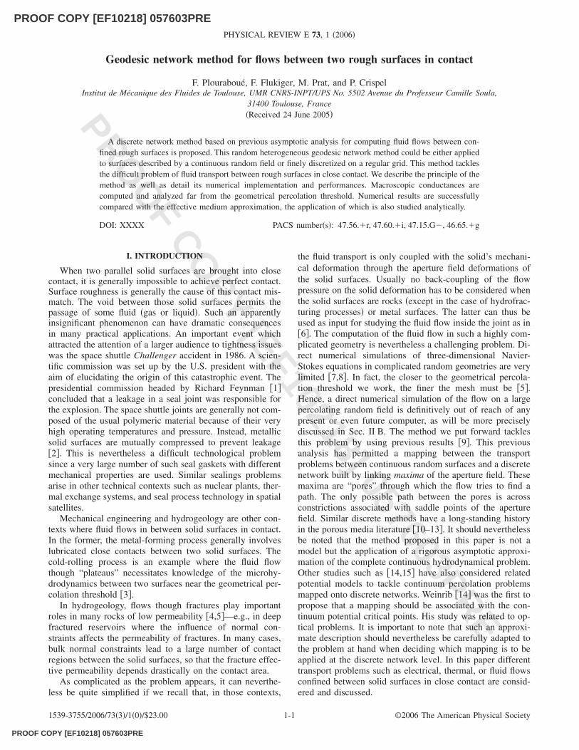
The only possible path between maxima crosses constric-tions associated with saddle points. Hence the geodesic net-work presented in the previous section is the topologicalskeleton of continuous paths linking the pore network. Thisskeleton is illustrated in Figs. 1 and 2. Let us first qualita-tively describe the evolution of the network structure whenthe surfaces are forced into close contact. To that purpose letus first define as “active” links �black lines in Fig. 1�b�� thoseassociated with nonzero local aperture. Nonactive links areassociated with contact regions where the local aperture isequal to zero �dotted lines in Fig. 1�a��. Given the total num-ber of links, Ltot, in the absence of any contact, there is asmaller number of active links, L�Lc, in the network due tothe contact region forced by nonzero values of the level setcriterion H in Eq. �3�.

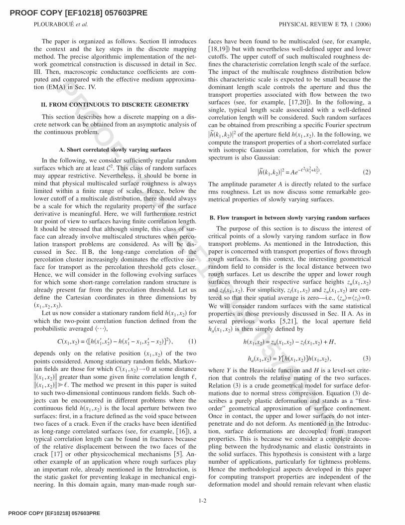
For a given critical Hc, the number of active links reachesa critical value Lc associated with the geometrical percola-tion threshold from boundary x2=0 to x2=2�. Below thiscritical value, there will be no percolating path from x2=0 tox2=2� on the graph network. Then, the usual parameter toconsider in order to quantify the distance to percolationthreshold is pL= �L−Lc� /Ltot. This parameter is the order pa-rameter of the percolation transition. When pL=0, the perco-lation threshold is reached. So the larger the values of pL, thefarther the geometrical percolation threshold. This could beobserved in the network structure represented in Fig. 2. Forvalues of pL as “large” as 0.25 the network structure looksreasonably homogeneous, while for values smaller than 0.1large holes can be observed associated with increasing cor-relation length of the percolation cluster of the contact re-

gions. It is interesting to note that the contact and noncontactregions are dual in two dimensions, so that the percolationthreshold for noncontact regions is the same as the one forcontact regions. An increasing correlation between contactregions thus has a direct impact on the induced increasingcorrelation of the active link network, which progressivelysmears out the preexisting finite correlation length �. Thisgeometrical transition from a homogeneous to highly hetero-geneous network has a direct impact on the transport prop-erties. This paper further investigates the transition betweenthe percolation regime and the breakdown of the mean-fieldapproximation for transport coefficients in Sec. IV.

When considering large-scale transport properties oneneeds a large number of correlation lengths along with spa-tially averaged transport properties. It is then clear that thenumerical representation of such continuous surfaces in-volves an even larger number of discrete elements. Comput-ing transport properties over this finely discretized surfaceover many correlation lengths rapidly becomes impossible.

A previous analysis �9� has shown that the local apertureof each saddle point controls the spatial discretization neces-sary for computing the flow field. The lower the saddle-pointaperture is, the smaller the spatial discretization should be.Hence tight constrictions associated with a very smallsaddle-point local aperture necessitate a challenging numberm of discretization points �as many as m=512 when using afinite-difference method of resolution for a ratio of apertureof the order of one-tenth between the saddle point and itsadjacent maxima �9��. These considerations make it clearthat the computational cost makes a direct computation ofthe flow unrealistic when the surface considered contains alarge number of correlation lengths. There is nevertheless away around this. A previous study �9� estimates the effectiveconductance of a continuous bond passing through a saddle-point between two maxima of the aperture field. This estima-tion obtained with matched asymptotic expansion providesan analytical estimate for conductances as a function of thesaddle-point local geometrical properties. This analysis thenpermits the mapping of three-dimensional continuous partial

FIG. 1. Schematic representation of the geodesic network. White regions are associated with contacts regions between the two surfaceswhere the local aperture is zero, while grey regions are those associated with nonzero aperture regions. Some level sets of the aperture mapare represented with dotted curves in those gray regions. The geodesic network linking maxima is represented with solid black lines, wherethe maxima are represented with grey solid circles. The saddle-point position along those geodesic network is represented with triangles. �a�All the links are represented. Active links are in black, and nonactive links are in grey. �b� Only the active links are represented.

GEODESIC NETWORK METHOD FOR FLOWS BETWEEN… PHYSICAL REVIEW E 73, 1 �2006�

1-3



PROO

F COPY [EF10218] 057603PRE

differential problems �i.e., harmonic and Stokes problems�on a slowly varying spatial aperture field onto the discretenetwork of maxima linked with effective conductance bonds.

Here we discuss the scaling of the “discrete mapping”asymptotic results with the saddle-point geometrical proper-ties. Let us consider the scalar field �n�x1 ,x2� associated withflow in between two rough surfaces. The scalar field �ncould be a pressure �n=3�, an electrical potential �n=1�, or atemperature �n=1�.

The mapping problem then consists in finding the equiva-lent conductance gn that could account for the local potentialloss ��n between two connected maxima, given the totalflux q that flows between those maxima. More precisely, thetotal flux q can be evaluated as the integral of the projectionof the scalar field potential gradient ��n �e.g., the pressuregradient for n=3� onto the normal to a surface defined at thesaddle point. This surface intersects the saddle point locatedat �x1s ,x2s� which connects the two maxima. It is defined byits normal which is parallel to the eigenvector of the Hessianmatrix whose eigenvalue H+�x1s ,x2s� is positive. Then thereis a linear relation between the flux and potential loss q=−gn��n /�n, where �n is a physical parameter that depends

on the problem under study; for n=1 it could either be theinverse of the fluid diffusivity or the inverse of the fluidelectrical conductivity; for n=3 it is the dynamic viscosity ofthe fluid. The conductance coefficient gn is then related to thelocal geometrical properties of the saddle point by the fol-lowing relation �the result �56� of Ref. �9� should have beenwritten in its dimensional formulation�:

gn = cn H+�x1s,x2s�− H−�x1s,x2s�

hn�x1s,x2s� , �4�

where H+�x1s ,x2s� and H−�x1s ,x2s� are the positive and nega-tive Hessian eigenvalues at the saddle point and cn is a con-stant coefficient. The eigenvalues H+ and H− are also theinverse of the positive and negative radii of curvature at thesaddle point from relation �A5�. In the following, all thesurfaces considered are normalized with root-mean-square�rms� roughness equal to 1. This is equivalent to nondi-mensionalizing the local conductances gn by n. Thus theresults associated with the macroscopic conductances Gn arealso nondimensionalized by n. The scaling obtained in re-lation �4� can be obtained with simple arguments. First, thedependence on the nth power of the local aperture field hn

can be simply derived from the previously mentioned lubri-cation results that the local conductance already scales as hn.The dependence on the square root of the radius of the cur-vature ratio also derives from this lubrication approximationproperty. It is worth noting that the effective conductancecould be expressed as the composition of parallel resistanceintegrated along the flow trajectories. In the vicinity of thesaddle point, these trajectories are locally parallel to the Hes-sian positive eigenvector direction. Let us call this directionx+. Because the potential drop is mainly controlled by rapidvariations localized in the vicinity of the saddle point, thetotal conductance along one trajectory can be approximatedby the composition of conductances in series along x+.Hence, integrating along all trajectories will introduce an-other composition of parallel conductances along the x− di-rection. Hence a formal evaluation of gn without explicitlyconsidering its prefactor is

gn � dx−1

� dx+1

hn�x+,x−�

. �5�

Now since, in the vicinity of the saddle point, the aperturefield has a quadratic shape, it can be approximated by

h�x+,x−� � h�x1s,x2s� +1

2H+�x1s,x2s�x+

2

+1

2H−�x1s,x2s�x−

2 + ¯ . �6�

Rescaling x+ as x+�=x+ /H+ and x− as x−�=x− /−H− then, oneeasily find from �5� and �6� that gn−H+ /H−. Hence eachscaling obtained in Eq. �4� can be found from simple argu-ments. The computation of the prefactor cn is much moredifficult and necessitates the use of matching asymptotictechniques. It was found in �9� that c1=2/3 and c3=1/14.

FIG. 2. Geodesic network for a N2=10242 discrete surface, withN /�=163 for six different values of the level set H of �3�. Associ-ated values of the parameter pL= �L−Lc� /Ltot are 0.45 in �a�, 0.35 in�b�, 0.25 in �c�, 0.15 in �d�, 0.1 in �e�, and 0 in �f�. The level-setvalues have been chosen so that �a� represents the original surfacenetwork with all its links, whereas �f� is the extreme case of thenetwork at percolation threshold. The same conventions as Fig. 1have been chosen to represent maxima with black circles, while thegeodesic network is drawn with solid black lines.


1-4



PROO

F COPY [EF10218] 057603PRE

The asymptotic validity of �5� was checked numerically in�9�. To that purpose, the small parameter which is the ratiobetween the saddle-point aperture and the local radius ofcurvature at the saddle point was systematically varied.More precisely defining this small parameter ash�x1s ,x2s�H+�x1s ,x2s�, Eq. �4� is the lowest-order estimateof the conductance in the asymptotic expansion involvingthis small parameter.

Surprisingly, it was found in �9� that the validity range ofthe proposed asymptotic approximation was quite broad.Equation �4� gives a reasonable estimate �to within 20%� ofthe conductance for values of the small parameter as large 3in the case n=3. The case n=1 is less favorable; still, thevalue of the small parameter could be as large as 1 for a 20%estimate, as obtained in �9� from numerical computation.

We have now described how the mapping of continuoustransport problems on critical points of the aperture fieldcould be obtained. Let us now discuss how the discrete map-ping is related to geometrical properties of slowly varyingrandom surfaces.

C. Principles of the geodesic network method

To map the continuous transport problem onto a discretenetwork, it is first interesting to consider the critical points ofthe surfaces. For any of these critical points, one can easilyretrieve maxima, minima, and saddle points. Each of these isfound from the property of the local Hessian matrix Hij=�ij

2 h at each critical point. The saddle points are those wherethe determinant of the Hessian matrix is negative: det H�0. Maxima are the points where det H0 and the trace ofthe Hessian matrix is negative, Tr H�0, while minima arethose for which det H0 and Tr H0. Among these ex-trema, saddle points play a particular role in the flow trans-port as discussed in Sec. III B. From the geometrical point ofview, saddle points are interesting for they are points whichconnect the shortest paths along the surface linking onemaximum to another cross section. Starting from one extre-mum to reach another one, the surface geodesics thus crossone saddle point. Hence, this property also occurs for theshortest paths linking minima which are orthogonal to geo-desics of the maxima at each saddle point. We will not con-sider the minima’s geodesic in the following, for reasons thatwill become obvious in the next section. We will rather con-centrate on the construction of the geodesic network of themaxima. Two maxima are considered “connected” if a geo-desic links them to the same saddle point. Figure 1 illustratesthis connection between maxima through saddle points on aspatially slowly varying surface. Geodesics are simpler tocompute on slowly varying surfaces than in the general casefor they coincide with steepest descent or steepest ascentpath as shown in the Appendix. We now briefly discuss thenumerical implementation of this discrete mapping method.

III. NUMERICAL IMPLEMENTATION

This section focuses on the numerical implementation ofthe method whose theoretical basis was discussed in the pre-vious section. Different algorithmic choices are possible. We

tried to find a compromise between computational efficiency,robustness, and simplicity. The implementation of themethod for the computation of macroscopic transport con-ductances follows different steps.

First critical points need to be found. From these, themaximum geodesic network must be computed in order tofind the bounds between maxima. Boundary conditions arethen applied to this biperiodic two-dimensional network. Forthat purpose, maxima linked with each boundary should beidentified. Then, for each level set H controlling the aperturefield �3� one needs to extract the percolating connected com-ponent of the network discrete graph. The part of the graphwhich is disconnected from the percolating component doesnot contribute to the flow transport. It is thus discarded. Wedescribe each of these steps in the following. Before giving amore detailed description of the algorithmic implementation,let us first add some important remarks. Numerically, one hasto discretize the field h�x1 ,x2� obtained from computing the

inverse Fourier transform of h̃�k1 ,k2� defined in �2� on a�0,2�� 0,2�� domain. Then we choose a ratio betweenthe typical correlation length � and the chosen discretization.The robustness of the following algorithm drastically de-pends on this discretization and on the precision required todefine saddle points. Some numerical estimates indicate thata spatial discretization larger than six points per correlationlength in the spectral representation gives a 10−8 relative er-ror on the critical point positions. This level of discretizationis implicitly considered in the following, while not beingrestrictive. Some of the algorithmic parameters have never-theless to be adapted to this arbitrary discretization. Let usnow discuss the different steps in more detail.

A. Aperture field generation and critical point determination

We use relation �2� to numerically generate surfaces asdescribed in �22�. The prescription of a suitable Hermitic

discretized complex field h̃�i , j� with i=1,N1, j=1,N2 inFourier space imposes a real discretized biperiodic fieldh�i , j� in direct space.

Then, the discrete field h�i , j� being defined, it is a classi-cal and nontrivial algorithmic problem to extract its criticalpoints. We chose a multigrid algorithm coupled with a clas-sical Newton-Picard method to identify critical points. First,fast-Fourier-transform techniques were used to compute thevector gradient �h�i , j� and Hessian matrix Hi,j fields of thediscrete random field h�i , j� on the Cartesian equispaced grid�i , j�. When needed on arbitrary points �x1 ,x2� in the plane,any field can be interpolated with an arbitrary polynomialprecision. We set quadratic interpolation degrees by default.Higher-order contributions of the polynomial order could beincreased if the Newton method research failed after somearbitrary number of steps �which is chosen equal to 80�. Af-ter convergence, the polynomial interpolation could also beincreased during a new search if the required precision is notreached. Nevertheless, in view of the first discretizationlevel, the required precision is always obtained with low in-terpolation order. The total number of extrema, ne, is directlyproportional to the chosen discretization, ne�N1N2, up to a


1-5



PROO

F COPY [EF10218] 057603PRE

prefactor that depends on the chosen correlation length �.The ratio N1N2 /ne is exactly equal to m2, the gain on dis-cretization when the network is used instead of the originalsurface. This ratio depends on the original discretizationlevel as well as on the correlation length. For reasonablediscretization levels, it reaches two orders of magnitude. Itwill be shown in the following that this is of considerableimportance for the flow computation.

B. Connecting critical points

Critical point characteristics are easily obtained from thedeterminant and trace of the Hessian matrix H, as alreadymentioned in Sec. II C. The connection between maxima ofthe field h is obtained from the computation of geodesicsstarting from each saddle point. This computation isachieved with a steepest ascent method starting from eachsaddle point. The convergence criterion to this maximum isthe same as the one used with the Newton search for criticalpoints. Nevertheless, when the step size becomes too small,the algorithm switches from the steepest ascent method tothe previous Newton search. This method provides verygood results for linking saddle points to their correspondingmaxima. The maximum-saddle-maximum triplet will becalled a link in the following. Considering the list of allmaxima, the computation of a new link connection will re-quire a search over the whole list of maxima. The cost of thissearch can be greatly reduced by using a bucket sort to struc-ture the list of maxima into a coarse bucket grid.

C. From continuous to discrete boundary conditions

Once the network is built, one has to map the continuousproblem boundary conditions onto the discrete network. Be-low, Dirichlet and periodic boundary conditions are consid-ered. The x1 direction has periodic boundary conditions,while constant Dirichlet potential boundary conditions areapplied along x2 at x2=0 and x2=2�. The network con-structed using the previously described method is biperiodic.It thus necessitates some modifications to take into accountthe Dirichlet boundary condition of the potential in the x2direction. Each periodized link crossing the lines x2=0 andx2=2� has to be considered. For each of these crossing links,we need to find the “inside” and “outside” maxima. This isdone by considering that the outside maximum is the one forwhich the x2 coordinate needs to be periodized. At this point,the inside maximum is assigned to the boundary under con-sideration �i.e., x2=0 or x2=2�� while the outside maximumis assigned to the other boundary �i.e., x2=2� or x2=0�.Hence, for each link crossing the boundary, two new linksare created, and the crossing link is suppressed from the linklist.

D. Graph operations on percolating clusters

The subsections above have discussed the network con-struction. This section gives a detailed presentation of theoperation needed on the discrete graph network to be able tocompute the flow transport onto the topological skeleton ofthe aperture network. These procedures are related to the

topology of the graph, while approaching the percolationthreshold.

One first needs to extract the connected component of thegraph network. This is achieved with a deep search algorithmimplemented following classical methods �23�.

The second step of graph operations is related to the iden-tification of percolating and nonpercolating connected com-ponents. The geometrical percolation criterion of the topo-logical skeleton is slightly different from the continuousaperture field. In the latter, the geometrical percolation isdefined by finding any continuous path from the x2=0 to thex2=2� boundaries. When a discrete representation h�i , j� ofthe aperture field is considered, this percolation criterion isdefined on site percolation along nonzero values of the Car-tesian grid h�i , j�. Now, transposing the geometrical percola-tion criterion onto the topological skeleton, one needs to con-sider bound percolation along the graph links which permitsa path from x2=0 to x2=2� to be found inside the graph.This procedure is applied for each imposed level-set criterionH until no path can be found for a threshold value Hc. Adichotomy iterative procedure on the level-set value H isused to find the critical Hc. Once again, a deep search algo-rithm was implemented to achieve this purpose.

Since they do not contribute to the transport properties,the dead ends of each percolating connected componentcould have been suppressed. This task is nevertheless unnec-essary because dead ends do not represent a large proportionof the network links; nor do they complicate the flow trans-port problem. On the contrary, the suppression of dead endsfrom the graph is technically involved �see, for example,�24�� and rather expensive algorithmically.

E. Solving the linear system for the potential computation

In Sec. III D we extracted the connected components ofpercolating clusters. The links that are related to boundariesx2=0 and x2=2� are also known from Sec. III C, as a sub-class of the percolating components sets. This subclass hasnow to be extracted from the link sets so that Dirichletboundary conditions can be applied. More precisely the po-tential �n has to be imposed so that �n�x1 ,0�=0 and�n�x1 ,2��=1. The corresponding set of boundary links canthen be used to construct the right-hand side of the linearsystem for computing the potential. On the left-hand side, therigidity matrix is built up from the sets of interior links usinga classical Kirchoff conservation law at each node �25�. Theuse of compact storage for the memory allocation of thesparse rigidity matrix makes for very low memory costs forsolving the linear system. A generalized minimal residualmethod preconditioned by a partial LU decomposition waschosen for the inversion of the linear system. This iterativemethod has been compared with a direct method near thepercolation threshold. The comparison is useful, because therigidity matrix is extremely ill conditioned, and it might hap-pen that the convergence accuracy could be poor. It turns outthat we did not find out any difference in the results up to thecomputer’s double-precision digits.

These numerical procedures allow the computation of thehydraulic conductances of joints having a large number N of


1-6



PROO

F COPY [EF10218] 057603PRE

correlation lengths in each �x ,y� direction. The computa-tional cost of the procedure has been drastically reduced sothat many statistical averages can be performed over the ob-tained results on a monoprocessor PC. The following sectionillustrates some of the numerical results obtained and theiranalysis, far from the percolation threshold.

IV. ANALYSIS OF TRANSPORT PROPERTIES FARFROM THE PERCOLATION THRESHOLD

This section investigates the macroscopic conductancesby the numerical method described in the previous sections.We first describe the effective medium approximation and itsuse for computing macroscopic conductances. We then dis-cuss the comparison between this approximation and directnumerical computations. We finally consider an analyticalapproximation of the EMA approach for the hydraulic effec-tive conductance G3.

A. Mean-field EMA

The EMA literature for scalar problems in heterogeneousmedia is very rich. We refer to �26� for a good recent over-view of this topic. Our interest in the present paper is toapply such a method to the problem of conductances be-tween two surfaces. As will be seen, this is an original prob-lem for which new results can be established. The main pointis to find good approximations for the effective macroscopicconductances, which will be denoted Gn in the followingwith n=1 or n=3. These macroscopic effective conductancesare associated with the discrete bound network of aperturemaxima described in the previous section. Along this discretebound network, local conductances are defined through �4�.Hence, one can compute the set of all local conductances gn�, averaged over different realizations, with the associatedprobability density function �PDF� p�gn�. Given the networkmean coordinance number z, the EMA then proposes an in-tegral equation formulation for the effective macroscopicconductances Gn:

�0

gn − Gn

gn + ZGnp�gn�dgn = 0, �7�

where the coefficient Z is related to the averaged coordinancenumber z by the simple relation Z=z /2−1. This formula iswritten in the limit of an infinite aperture field h�x1 ,x2�.Hence, the value of Z should be evaluated on an infinitesurface. This is obviously not possible in practice becausephysical objects have a finite number of correlation lengths.A good approximation is thus to compute z for a large butfinite number of correlation lengths. Numerical estimates aregiven the values in Table I.

The statistical fluctuations associated with the averagedresults of Table I are lower than the given number of digits.The PDF p�gn� distribution associated with the local conduc-tances describes both “active” links �black lines on Fig.1�b��, for which the local aperture is nonzero, and “nonac-tive” ones associated with contact regions with zero localaperture �dotted lines in Fig. 1�a��. Given the total number of

links, Ltot, and the total number of active links, L, the PDFcan be decomposed, so that

p�gn� = �1 − Fa��0� + Fapa�gn� , �8�

where Fa=L /Ltot denotes the fraction of active links whosePDF distribution is pa�gn�. Using Eq. �8� to describe the re-lation between the macroscopic conductance and the PDFdistribution of active links in Eq. �7� it is easy to find that

�0

gn − Gn

gn + ZGnpa�gn�dgn =

�1 − Fa�ZFa

. �9�

Far from the percolation threshold, this relation should give agood approximation of the macroscopic conductance. It istherefore an interesting method to compare with direct nu-merical computations obtained from the method described inthe previous section. This method nevertheless requiresknowledge of the active link PDF pa�gn�. This PDF can becomputed numerically over a large number of local conduc-tances obtained from relation �4�. Let us first discuss thenumerical evaluation of EMA macroscopic conductances.

B. Numerical evaluation of the EMA and comparisonwith numerical computations

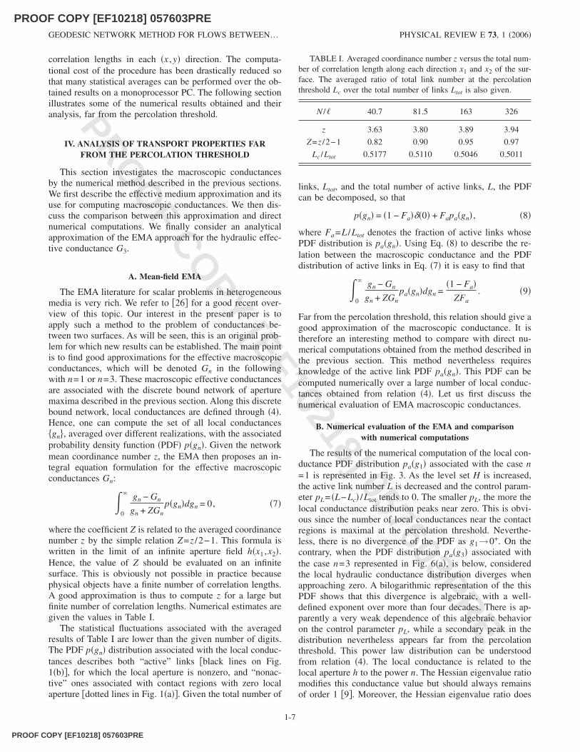
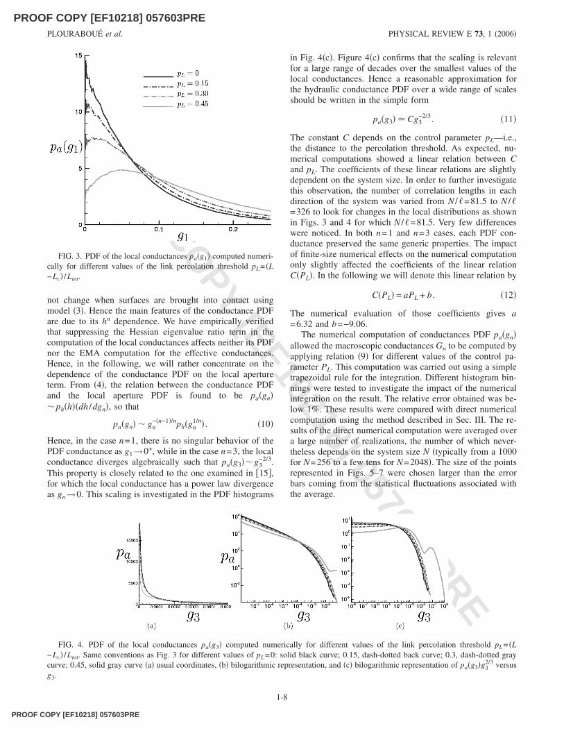
The results of the numerical computation of the local con-ductance PDF distribution pa�g1� associated with the case n=1 is represented in Fig. 3. As the level set H is increased,the active link number L is decreased and the control param-eter pL= �L−Lc� /Ltot tends to 0. The smaller pL, the more thelocal conductance distribution peaks near zero. This is obvi-ous since the number of local conductances near the contactregions is maximal at the percolation threshold. Neverthe-less, there is no divergence of the PDF as g1→0+. On thecontrary, when the PDF distribution pa�g3� associated withthe case n=3 represented in Fig. 6�a�, is below, consideredthe local hydraulic conductance distribution diverges whenapproaching zero. A bilogarithmic representation of the thisPDF shows that this divergence is algebraic, with a well-defined exponent over more than four decades. There is ap-parently a very weak dependence of this algebraic behavioron the control parameter pL, while a secondary peak in thedistribution nevertheless appears far from the percolationthreshold. This power law distribution can be understoodfrom relation �4�. The local conductance is related to thelocal aperture h to the power n. The Hessian eigenvalue ratiomodifies this conductance value but should always remainsof order 1 �9�. Moreover, the Hessian eigenvalue ratio does

TABLE I. Averaged coordinance number z versus the total num-ber of correlation length along each direction x1 and x2 of the sur-face. The averaged ratio of total link number at the percolationthreshold Lc over the total number of links Ltot is also given.

N /� 40.7 81.5 163 326

z 3.63 3.80 3.89 3.94

Z=z /2−1 0.82 0.90 0.95 0.97

Lc /Ltot 0.5177 0.5110 0.5046 0.5011


1-7



PROO

F COPY [EF10218] 057603PRE

not change when surfaces are brought into contact usingmodel �3�. Hence the main features of the conductance PDFare due to its hn dependence. We have empirically verifiedthat suppressing the Hessian eigenvalue ratio term in thecomputation of the local conductances affects neither its PDFnor the EMA computation for the effective conductances.Hence, in the following, we will rather concentrate on thedependence of the conductance PDF on the local apertureterm. From �4�, the relation between the conductance PDFand the local aperture PDF is found to be pa�gn� ph�h��dh /dgn�, so that

pa�gn� gn−�n−1�/nph�gn

1/n� . �10�

Hence, in the case n=1, there is no singular behavior of thePDF conductance as g1→0+, while in the case n=3, the localconductance diverges algebraically such that pa�g3�g3

−2/3.This property is closely related to the one examined in �15�,for which the local conductance has a power law divergenceas gn→0. This scaling is investigated in the PDF histograms

in Fig. 4�c�. Figure 4�c� confirms that the scaling is relevantfor a large range of decades over the smallest values of thelocal conductances. Hence a reasonable approximation forthe hydraulic conductance PDF over a wide range of scalesshould be written in the simple form

pa�g3� � Cg3−2/3. �11�

The constant C depends on the control parameter pL—i.e.,the distance to the percolation threshold. As expected, nu-merical computations showed a linear relation between Cand pL. The coefficients of these linear relations are slightlydependent on the system size. In order to further investigatethis observation, the number of correlation lengths in eachdirection of the system was varied from N /�=81.5 to N /�=326 to look for changes in the local distributions as shownin Figs. 3 and 4 for which N /�=81.5. Very few differenceswere noticed. In both n=1 and n=3 cases, each PDF con-ductance preserved the same generic properties. The impactof finite-size numerical effects on the numerical computationonly slightly affected the coefficients of the linear relationC�PL�. In the following we will denote this linear relation by

C�PL� = aPL + b . �12�

The numerical evaluation of those coefficients gives a=6.32 and b=−9.06.

The numerical computation of conductances PDF pa�gn�allowed the macroscopic conductances Gn to be computed byapplying relation �9� for different values of the control pa-rameter PL. This computation was carried out using a simpletrapezoidal rule for the integration. Different histogram bin-nings were tested to investigate the impact of the numericalintegration on the result. The relative error obtained was be-low 1%. These results were compared with direct numericalcomputation using the method described in Sec. III. The re-sults of the direct numerical computation were averaged overa large number of realizations, the number of which never-theless depends on the system size N �typically from a 1000for N=256 to a few tens for N=2048�. The size of the pointsrepresented in Figs. 5–7 were chosen larger than the errorbars coming from the statistical fluctuations associated withthe average.

FIG. 3. PDF of the local conductances pa�g1� computed numeri-cally for different values of the link percolation threshold pL= �L−Lc� /Ltot.

FIG. 4. PDF of the local conductances pa�g3� computed numerically for different values of the link percolation threshold pL= �L−Lc� /Ltot. Same conventions as Fig. 3 for different values of pL=0: solid black curve; 0.15, dash-dotted back curve; 0.3, dash-dotted graycurve; 0.45, solid gray curve �a� usual coordinates, �b� bilogarithmic representation, and �c� bilogarithmic representation of pa�g3�g3

2/3 versusg3.


1-8



PROO

F COPY [EF10218] 057603PRE

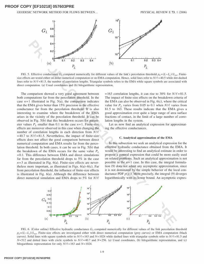
The comparison showed a very good agreement betweenboth computations far from the percolation threshold. In thecase n=1 illustrated in Fig. 5�a�, the comparison indicatesthat the EMA gives better than 15% precision in the effectiveconductance far from the percolation threshold. It is alsointeresting to examine where the breakdown of the EMAarises in the vicinity of the percolation threshold. It can beobserved in Fig. 5�b� that this breakdown occurs for param-eter values PL smaller than 0.1 in the case n=1. Finite-sizeeffects are moreover observed in this case when changing thenumber of correlation lengths in each direction from N /�=40.7 to N /�=81.5. Nevertheless, the impact of finite-sizeeffects does not affect the good comparison between directnumerical computation and EMA results far from the perco-lation threshold. In both cases, it can be see in Fig. 5�b� thatthe breakdown of the EMA occurs for the same value PL=0.1. This difference between EMA and direct simulationsfar from the percolation threshold drops to 5% in the casen=3 as illustrated in Fig. 6�a�. Finite-size effects are never-theless more important, as illustrated in Figs. 6�a�–6�c�. Farfrom percolation threshold, the influence of finite-size effectsis illustrated in Fig. 6�a�. Although the difference betweendirect numerical simulation and EMA drops to 5% for N /�

=163 correlation lengths, it can rise to 30% for N /�=81.5.The impact of finite-size effects on the breakdown criteria ofthe EMA can also be observed in Fig. 6�c�, where the criticalvalue for PL varies from 0.05 to 0.1 when N /� varies from81.5 to 163. These results indicate that the EMA gives agood approximation over quite a large range of area surfacefractions of contact, in the limit of a large number of corre-lation lengths in the system.

Let us now find an analytical expression for approximat-ing the effective conductances.

C. Analytical approximation of the EMA

In this subsection we seek an analytical expression for theeffective hydraulic conductance obtained from the EMA. Itwould be interesting to find an analytical estimate in order topropose a general expression that could be more easily usedon related problems. Such an analytical approximation is notpossible in the n=1 case. In this case, the integral formula-tion �9� does not admit any asymptotic approximation, sinceit is not dominated by the simple behavior of the local con-ductance PDF p�g1�. More precisely, the integral �9� divergeslogarithmically with its lower bound. An asymptotic expres-

FIG. 5. Effective conductance G1 computed numerically for different values of the link’s percolation threshold pL= �L−Lc� /Ltot. Finite-size effects are tested either on direct numerical computation or on EMA computation. Hence, solid lines refer to N /�=40.5 while dot-dashedlines refer to N /�=81.5, the number of correlation lengths. Triangular symbols refers to the EMA while square symbols are associated withdirect computation. �a� Usual coordinates and �b� bilogarithmic representation,

FIG. 6. �Color online� Effective hydraulic conductance G3 computed numerically for different values of the link percolation thresholdpL= �L−Lc� /Ltot. Finite-size effects are investigated either with direct numerical computation �grey curves� or EMA computation �blackcurves�. Solid lines with square symbols refer to N /�=163 and N=1024 while dashed lines with triangular symbols refer to N /�=81.5 andN=512 and dotted lines with circle symbols to N /�=40.7 and N=256. �a� Usual coordinates, �b� bilogarithmic representation, and �c�bilogarithmic representation for only N /�=163 and N=1024.


1-9



PROO

F COPY [EF10218] 057603PRE

sion of the integral as a function of the lower bound can befound but the contribution of the upper bound cannot beneglected. It turns out that no closed form can be found forG1 as a function of the lower and upper bounds in that case.

In contrast, in the case n=3, the simple behavior of thelocal conductance PDF p�g3� expressed in relation �11�dominates the left-hand-side integral of relation �9�. Thelower and upper integral bounds should nevertheless beequal to 0 and 1/ �3C�3, so that PDF �11� is normalized onthis interval. Using those integral bounds and �11� in theleft-hand-side integral of relation �9� leads to an implicit andcumbersome relation that relates the effective conductancesG3 to C ,Z and obviously Fa=L /Ltot:

3X�1/Fa − 1 − Z��1 + Z�

=1

2ln�1 −

3X

�1 + X�2� − 3 arctan�2X − 13

�−

�3

6, �13�

where 1/X=3C�ZG3�1/3. This relation can be further simpli-fied by using the fact that the effective conductance G3 isalways quite small—i.e., G3�1—whatever value of the con-trol parameter Fa=L /Ltot�1 is. Thus, we seek an asymptoticexpansion of relation �13� as X�1. Keeping with O�1/X2�and discarding O�1/X4�, the right-hand side of Eq. �13� canbe expanded to give

3X�1/Fa − 1 − Z��1 + Z�

=1

2�−

3

X+

3

2X2� − 3��

2−

3

2X−

3

4X2�−

�3

6. �14�

From Eq. �14�, it can be seen that the root of the followingcubic equation gives an approximate expression for the ef-fective conductance:

X33�1/Fa − 1 − Z�1 + Z

+ X22�

3−

3

2= 0. �15�

An explicit solution for X and thus for G3 can be obtained bycomputing the smallest positive root of this cubic equation.This leads to the following explicit analytical expression:

G3 = −813�1/Fa − 1 − Z�3

8�3C3�1 + Z�3Z�1 + cos��/3� + sin��/3��3 ,

G3 = −813�1/�PL + Lc/Ltot� − 1 − Z�3

8�3C3�1 + Z�3Z�1 + cos��/3� + sin��/3��3 , �16�

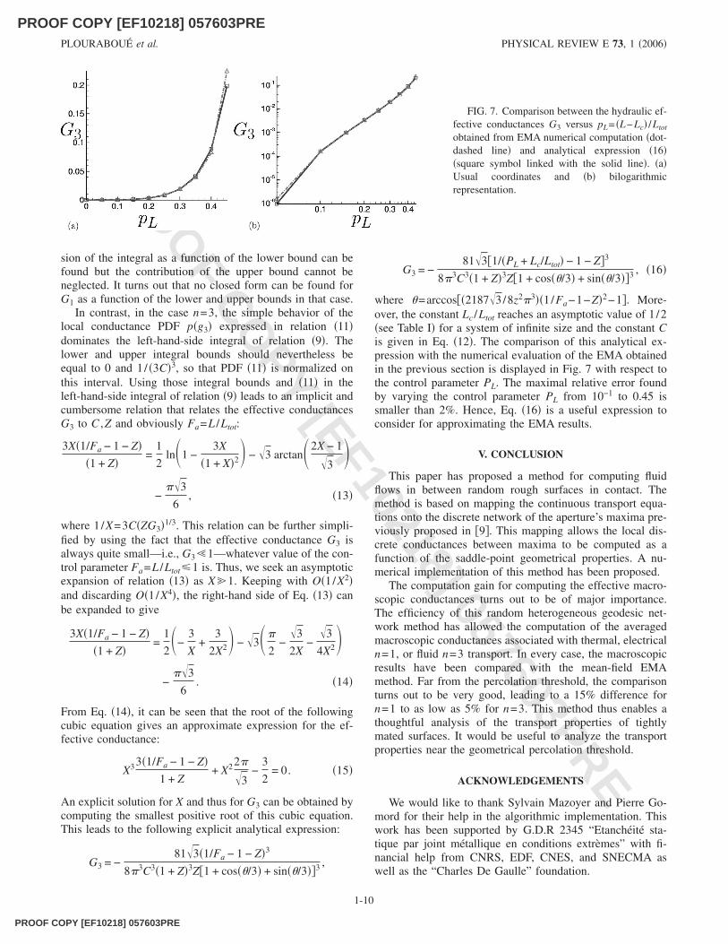
where �=arccos��21873/8z2�3��1/Fa−1−Z�2−1�. More-over, the constant Lc /Ltot reaches an asymptotic value of 1 /2�see Table I� for a system of infinite size and the constant Cis given in Eq. �12�. The comparison of this analytical ex-pression with the numerical evaluation of the EMA obtainedin the previous section is displayed in Fig. 7 with respect tothe control parameter PL. The maximal relative error foundby varying the control parameter PL from 10−1 to 0.45 issmaller than 2%. Hence, Eq. �16� is a useful expression toconsider for approximating the EMA results.

V. CONCLUSION

This paper has proposed a method for computing fluidflows in between random rough surfaces in contact. Themethod is based on mapping the continuous transport equa-tions onto the discrete network of the aperture’s maxima pre-viously proposed in �9�. This mapping allows the local dis-crete conductances between maxima to be computed as afunction of the saddle-point geometrical properties. A nu-merical implementation of this method has been proposed.

The computation gain for computing the effective macro-scopic conductances turns out to be of major importance.The efficiency of this random heterogeneous geodesic net-work method has allowed the computation of the averagedmacroscopic conductances associated with thermal, electricaln=1, or fluid n=3 transport. In every case, the macroscopicresults have been compared with the mean-field EMAmethod. Far from the percolation threshold, the comparisonturns out to be very good, leading to a 15% difference forn=1 to as low as 5% for n=3. This method thus enables athoughtful analysis of the transport properties of tightlymated surfaces. It would be useful to analyze the transportproperties near the geometrical percolation threshold.

ACKNOWLEDGEMENTS

We would like to thank Sylvain Mazoyer and Pierre Go-mord for their help in the algorithmic implementation. Thiswork has been supported by G.D.R 2345 “Etanchéité sta-tique par joint métallique en conditions extrèmes” with fi-nancial help from CNRS, EDF, CNES, and SNECMA aswell as the “Charles De Gaulle” foundation.

FIG. 7. Comparison between the hydraulic ef-fective conductances G3 versus pL= �L−Lc� /Ltot

obtained from EMA numerical computation �dot-dashed line� and analytical expression �16��square symbol linked with the solid line�. �a�Usual coordinates and �b� bilogarithmicrepresentation.


1-10



PROO

F COPY [EF10218] 057603PRE

APPENDIX: GEODESIC NETWORK OF CRITICALPOINTS ON SLOWLY VARYING ROUGH SURFACES

This appendix shows how the curvature tensor defined onevery point of a smooth C2 surface can be approximated bythe Hessian matrix. From this approximation, it is shownhow to construct the geodesic network linking all criticalpoints by following steepest descent path along the surface.

Smooth short-correlated surfaces have well-defined criti-cal points where the surface height gradient vanishes. Moreprecisely let us first briefly discuss the properties of surfaceshaving slow variations in the �x1 ,x2� horizontal directionsassociated with a small parameter �. Any point defined by itsvector position x= �x1 ,x2 ,x3� in three dimensions and locatedon a slowly varying surface S defined as x3=h��x1 ,�x2� hascoordinates x= �x1 ,x2 ,h�. Critical points are those for which

� �h

�x1,

�h

�x2� = �0,0� . �A1�

It is now interesting to introduce slowly varying coordinates�X1=�x1, X2=�x2� so that the surface variations are now ex-pressed directly by x3=h�X1 ,X2�. Let us denote the partialderivative � /�Xi with respect to the slow Cartesian coordi-nate Xi, �i, with i=1,2, and let us define �h= ��1h ,�2h�.Condition �A1� can now be expressed by

�h = ��1h,�2h� =1

�� h

�x1,

�h

�x2� = �0,0� . �A2�

It is easy to see that, for a slowly varying surface, the localcurvature tensor coincides with the surface Hessian. Let usdefine the tangent vector to the surface by ��1x�x1= �1,0 ,��1h�, �2x�x2= �0,1 ,��2h��. The outward-orientednormal n to the surface then reads

n =x1 � x2

�x1 � x2�=

11 + �2 � h2

��1h,��2h,1� ,

n = ��1h,��2h,1� + O��2� , �A3�

where � denotes the vector product between two vectors inthree dimensions. The curvature tensor b is then defined inits two-covariant form as �see, for example, �27��

bij = − xi · n j with i = �1,2�, j = �1,2� , �A4�

where · denotes the scalar product between two vectors inthree dimensions and n j is �n /�Xj, j=1,2. Using �A3� thecurvature tensor given in �A4� can easily be computed up toO��2� terms as

bij = − ��ij2 h = − �Hij . �A5�

Hence, in this case, the principal curvature directions associ-ated with the eigenvectors of the curvature tensor are alwayslocally tangent to the Hessian eigenvectors. It is now easy torealise that, self-consistently, the steepest ascent path fromone saddle point to its adjacent maximum will follow a geo-desic of the smooth surface. The trajectory of any pointalong the surface is parametrized by time t. The steepestascent path along the surface is defined for any surface pointsby the local variation d�x1 ,x2� /dt=��h. The parameter t canbe prescribed to be equal to the third coordinate x3 along thesurface. Steepest ascent trajectories thus satisfy dx /dt= ��h ,1� in three dimensions, which from �A3�, leads todx /dt=n neglecting O��2� terms. Hence the tangent kine-matic vector along the steepest ascent trajectory is alwaysparallel to the surface normal. This is precisely the definitionof a geodesic. Hence, steepest ascent trajectories are surfacegeodesics on slowly varying smooth surfaces. This propertyis be used in Sec. III B to compute the geodesic networklinking all maxima of the surface.

�1� W. P. Rogers et al., The Presidential Commission on the SpaceShuttle Challenger Accident Report, Tech. rep., NASA �June 6,1986�.

�2� J. Martin �unpublished�.�3� N. Marsault, P. Montmitonnet, P. Deneuville, and P. Gratacos

�unpublished�.�4� K. J. Evans, T. Kohl, R. J. Hopkirk, and L. Rybach �unpub-

lished�.�5� P. Adler and J. Thovert, Fractures and Fracture Networks

�Kluwer Academic, Amsterdam, 1999�.�6� V. V. Mourzenko, O. Galamay, J. F. Thovert, and P. M. Adler,

Phys. Rev. E 56, 3167 �1997�.�7� D. Lo Jacono, F. Plouraboué, and A. Bergeon, Phys. Fluids 17,

063602 �2005�.�8� V. V. Mourzenko, J. F. Thovert, and P. M. Adler, J. Phys. II 5,

465 �1995�.�9� F. Plouraboué, S. Geoffroy, and M. Prat, Phys. Fluids 16, 615

�2004�.�10� M. B. Isichenko, Rev. Mod. Phys. 64, 961 �1992�.�11� J. Koplik, Disorder and Mixing �Kluwer, Dordrecht, 1988�, pp.

123–137.�12� M. Sahimi, Rev. Mod. Phys. 65, 1393 �1993�.�13� M. Sahimi, Flow and Transport in Porous media and Frac-

tured Rock �VCH Wienheim, New York, 1995�.�14� A. Weinrib, Phys. Rev. B 26, 1352 �1982�.�15� S. Feng, B. I. Halperin, and P. N. Sen, Phys. Rev. B 35, 197

�1987�.�16� S. R. Brown and C. H. Scholz, J. Geophys. Res. 90, 12 �1985�.�17� F. Plouraboué, P. Kurowski, J. P. Hulin, S. Roux, and J.

Schmittbuhl, Phys. Rev. E 51, 1675 �1995�.�18� A. Majumdar and B. Bhushan, ASME J. Tribol. 112, 205

�1990�.�19� F. Plouraboué and M. Boehm, Tribol. Int. 32, 45 �1999�.�20� F. Plouraboué, P. Kurowski, J. Boffa, J. P. Hulin, and S. Roux,

J. Contam. Hydrol. 46, 295 �2000�.�21� M. Prat, N. Letalleur, and F. Plouraboué, Transp. Porous

Media 48, 291 �2002�.�22� H. A. Makse, S. Havlin, M. Schwartz, and H. E. Stanley, Phys.

Rev. E 53, 5445 �1996�.�23� R. Tarjan, Data Structures and Network Algorithms �Society


1-11



PROO

F COPY [EF10218] 057603PRE

for Industrial and Applied Mathematics, New York, 1983�.�24� H. J. Herrmann, D. C. Hong, and H. E. Stanley, J. Phys. A 17,

L261 �1984�.�25� S. V. Patankar, Numerical Heat Transfer and Fluid Flow

�Hemisphere, ��, 1980�.

�26� J. Torquato, Random Heterogeneous Material �Springer-Verlag, Berlin, 2001�.

�27� T. Frankel, The Geometry of Physics: An Introduction �Cam-bridge University Press, Cambridge, England, 1997�.


1-12


Geodesic network method for flows between two rough surfaces in contact

Documents