Département fédéral de l’environnement, des transports, de l’énergie et de la communication DETEC Office fédéral de l’énergie OFEN Rapport final 30 juin 2011 Geocooling Handbook Cooling of Buildings using Vertical Borehole Heat Exchangers

Welcome message from author
This document is posted to help you gain knowledge. Please leave a comment to let me know what you think about it! Share it to your friends and learn new things together.
Transcript

Département fédéral de l’environnement, des transports, de l’énergie et de la communication DETEC
Office fédéral de l’énergie OFEN
Rapport final 30 juin 2011
Geocooling Handbook Cooling of Buildings using Vertical Borehole Heat Exchangers

Mandant: Office fédéral de l’énergie OFEN Programme de recherche géothermie CH-3003 Berne www.bfe.admin.ch Cofinancement: SUPSI – DACD – ISAAC, CH-6952 Canobbio
Mandataire: SUPSI – DACD – ISAAC Campus Trevano CH-6952 Canobbio www.isaac.supsi.ch
Auteurs: Daniel Pahud, SUPSI – DACD – ISAAC, [email protected] Marco Belliardi, SUPSI – DACD – ISAAC, [email protected]
Responsable de domaine de l’OFEN: Gunter Siddiqi Chef de programme de l’OFEN: Rudolf Minder Numéro du contrat et du projet de l’OFEN: 151’549 / 101’295
Les auteurs de ce rapport portent seuls la responsabilité de son contenu et de ses conclusions.

Impressum
iii
Riassunto In questo progetto si esamina in dettaglio il raffreddamento con geocooling di edifici amministrativi mediante sonde geotermiche verticali. L’analisi è incentrata sull’interazione termica tra l’edificio e l’installazione tecnica accoppiata al terreno, senza dimenticare la dinamica della distribuzione dell’energia di riscaldamento e di raffreddamento. Questo studio beneficia dei risultati di studi precedenti e di programmi di simulazione realizzati per applicazioni di installazioni con sonde geotermiche verticali.
È definito ed utilizzato come caso di riferimento un edificio amministrativo a basso consumo energetico. Si è stabilita una metodologia dettagliata per l’analisi degli edifici ed il dimensionamento delle installazioni basate sul geocooling. Vengono studiate le caratteristiche dell’edificio e le condizioni climatiche. Inoltre si utilizzano dei dati climatici corrispondenti sia al nord che al sud delle Alpi. Si è quindi analizzata la sensibilità del dimensionamento del campo di sonde geotermiche rispetto ai parametri più influenti.
Per analizzare i risultati di tutte le simulazioni, vengono proposte delle definizioni di chiavi di dimensionamento e dei coefficienti di capacità di trasferimento termico per il riscaldamento ed il raffreddamento. Queste forniscono delle regole semplici e veloci per ottenere un pre-dimensionamento di un’installazione basata sul geocooling mediante sonde geotermiche verticali.
Lo sviluppo dell’edificio ha un’influenza molto forte sul dimensionamento dell’installazione del geocooling. I casi studiati mostrano che l’utilizzo di finestre con vetri tripli, anziché vetri doppi, permettono di dimezzare la lunghezza totale delle sonde geotermiche. Le condizioni necessarie per la fattibilità e l’efficienza energetica di un’installazione con il geocooling sono: un concetto a basso consumo energetico, delle protezioni solari che rispettino le esigenze della norma svizzera SIA 382/1, dei guadagni termici interni che non eccedano sensibilmente oltre i valori standard relativi ad un edificio amministrativo tipico e così via. Queste condizioni rendono in linea di principio possibile l’uso di solette termoattive per il riscaldamento ed il raffreddamento dell’edificio. La deumidificazione dell’aria, se deve essere effettuata, è limitata al ricambio minimo di nuova aria per soddisfare le esigenze di qualità dell’aria interna. In questo caso il sistema di ventilazione è unicamente utilizzato per coprire i fabbisogni di raffreddamento di energia latente e non è connesso all’installazione tecnica accoppiata al terreno.
Una distribuzione del calore mediante le solette termoattive è la soluzione più adatta per minimizzare le quantità di energia distribuite per il riscaldamento ed il raffreddamento. Le loro proprietà autoregolanti sono un fattore determinante per evitare il conflitto “riscaldamento – raffreddamento” durante la mezza stagione. Permettendo di raffreddare con delle temperature elevate dell’acqua (più di 20°C), sono inoltre le più indicate per un’applicazione basata sul geocooling.
Uno dei parametri più influenti sulla lunghezza totale delle sonde geotermiche è il tasso di ricarica stagionale del terreno. Le installazioni più interessanti che sfruttano il geocooling presentano un tasso di ricarica del terreno di circa il 50%. Delle buone installazioni sono ottenute con un tasso di ricarica compreso tra il 40% e l’80%. Supponendo una conduttività termica del terreno di 2 W/mK e delle sonde posizionate sotto l’edificio, dei valori tipici per le chiavi di dimensionamento sono :
criterio per il riscaldamento : 25 – 35 W/m relativamente alla potenza nominale di estrazione.
criterio per il geocooling : 30 – 50 W/m relativamente alla potenza massima di raffreddamento distribuita
Un altro parametro chiave che condiziona fortemente il potenziale di geocooling è la differenza di temperatura tra la temperatura nominale di partenza del fluido nella distribuzione del raffreddamento e la temperatura iniziale del terreno. Il potenziale di geocooling aumenta quando la temperatura di partenza è più elevata.

Impressum
iv
Viene quindi definito un coefficiente di capacità di trasferimento termico, sulla base della chiave di dimensionamento, per prendere in considerazione la differenza di temperatura disponibile. Un approccio simile viene allo stesso modo applicato alle chiavi di dimensionamento per il riscaldamento. I coefficienti di capacità di trasferimento termico che derivano dalle chiavi di dimensionamento sono:
criterio per il riscaldamento : 2 – 3 W/m/K relativamente alla potenza di estrazione nominale.
criterio per il geocooling : 6 – 7 W/m/K relativamente alla potenza di raffreddamento massima distribuita
Vengono calcolati alcuni esempi per mostrare l’utilizzo delle regole definite per predimensionare il campo di sonde geotermiche di una installazione con geocooling. È tuttavia importante avere la possibilità di simulare, siccome non è possibile stabilire delle regole di dimensionamento universali. Come risultato di questo progetto di ricerca, è disponibile il programma di simulazione COOLSIM2 per dei nuovi studi riguardanti installazioni con geocooling.
Impressum
v
Résumé Le rafraîchissement de bâtiments administratifs par geocooling sur sondes géothermiques verticales est examiné en détail dans ce projet. L’analyse est centrée sur l’interaction thermique entre le bâtiment et l’installation technique couplée au terrain, sans oublier la dynamique de la distribution d’énergie de chauffage et de refroidissement. Cette étude bénéficie des résultats d’études précédentes et d’outils de simulation réalisés dans le cadre d’applications d’installations avec sondes géothermiques verticales.
Un bâtiment administratif à basse consommation d’énergie est défini et utilisé comme cas de référence. Une méthodologie détaillée est établie pour l’analyse des bâtiments et le dimensionnement d’installations basées sur le geocooling. Les caractéristiques du bâtiment et les conditions climatiques sont étudiées. Aussi bien des données météorologiques du nord que du sud des Alpes sont utilisées. La sensibilité du dimensionnement du champ de sondes géothermiques aux paramètres les plus influents est analysée.
Des définitions de clefs de dimensionnement et de coefficients de capacité de transfert thermique pour le chauffage et le refroidissement sont proposées pour analyser les résultats de toutes les simulations. Elles fournissent des règles simples et rapides pour obtenir un pré-dimensionnement d’une installation basée sur le geocooling avec sondes géothermiques verticales.
L’enveloppe du bâtiment a une influence très forte sur le dimensionnement de l’installation de geocooling. Les cas étudiés montrent que l’utilisation de fenêtres triple-vitrages plutôt que double-vitrages permet de diminuer par deux la longueur totale des sondes géothermiques. Des conditions nécessaires pour la faisabilité et l’efficacité énergétique d’une installation de geocooling sont : un concept énergétique à basse consommation, des protections solaires qui respectent les exigences de la norme Suisse SIA 382/1, des gains thermiques internes qui n’excèdent pas sensiblement les valeurs standards relatives à un bâtiment administratif typique et ainsi de suite. Ces conditions rendent en principe possible l’utilisation de dalles actives pour le chauffage et le refroidissement du bâtiment. La déshumidification de l’air, si elle doit être faite, est limitée au renouvellement d’air neuf minimum pour satisfaire les exigences de qualité de l’air intérieur. Dans ce cas le système de ventilation est uniquement utilisé pour couvrir les besoins de refroidissement par énergie latente et il n’est pas connecté à l’installation technique couplée au terrain.
Une distribution d’énergie par dalles actives est la solution la plus adaptée pour minimiser les quantités d’énergie distribuées pour le chauffage et le refroidissement. Leurs propriétés auto-régulatrices sont un facteur déterminant pour éviter le conflit « chauffage – refroidissement » durant la mi-saison. Permettant de refroidir avec des températures d’eau élevées (plus de 20°C), elles sont ainsi les plus indiquées pour une application basée sur le geocooling.
Un des paramètres les plus influents sur la longueur totale de sondes géothermiques est le taux de recharge saisonnier du terrain. Les installations de geocooling les plus intéressantes sont obtenues avec un taux de recharge du terrain d’environ 50%. De bonnes installations sont obtenues avec un taux de recharge compris ente 40 et 80%. En supposant une conductivité thermique du terrain de 2 W/(mK) et des sondes géothermiques placées sous le bâtiment, des valeurs typiques de clefs de dimensionnement sont :
Critère de chauffage : 25 – 35 W/m relativement à la puissance d’extraction nominale. Critère de geocooling: 30 – 50 W/m relativement à la puissance de refroidissement maximum
distribuée
Un autre paramètre clef qui conditionne fortement le potentiel de geocooling est la différence de température entre la température de départ nominale du fluide dans la distribution de refroidissement et la température initiale du terrain. Le potentiel de geocooling est d’autant plus grand que la température de départ est plus haute. Un coefficient de capacité de transfert thermique est défini sur la base de la clef de dimensionnement pour prendre en compte la différence de température disponible. Une approche similaire est également appliquée aux clefs de

Impressum
vi
dimensionnement pour le chauffage. Les coefficients de capacité de transfert thermique qui dérivent des clefs de dimensionnement sont :
Critère de chauffage : 2 – 3 W/m/K relativement à la puissance d’extraction nominale. Critère de geocooling: 6 – 7 W/m/K relativement à la puissance de refroidissement maximum
distribuée
Quelques exemples sont calculés pour illustrer l’utilisation des règles établies pour pré-dimensionner le champ de sondes géothermiques d’une installation de geocooling. Il est toutefois important d’avoir la possibilité de simuler, car il n’est pas possible d’établir des règles de dimensionnement universelles. Comme produit dérivé de ce projet de recherche, l’outil de simulation COOLSIM2 est disponible pour de nouvelles études d’installations de geocooling.

Impressum
vii
Summary Geocooling systems with borehole heat exchangers integrated in office buildings are examined. The analysis is focused on the thermal interaction between the building and the ground coupled system, heating and cooling distribution included. This study takes advantage of previous studies and simulation tools made in the field of borehole heat exchanger applications.
A low energy office building is defined and used as a reference. A detailed methodology is established for building analysis and geocooling system sizing. Building design as well as weather data are studied, using climate data of both north and south side of the Alps. Sensitivity to the main sizing parameters of the ground coupled system is analysed.
Definitions of sizing keys and capacity values for heating and geocooling are proposed to analyse the results of all simulations. They provide simple and fast design guidelines for a pre-sizing of a geocooling system.
The building envelope has a strong influence on the geocooling system sizing. Most of the studied cases showed that triple instead of double glazing windows enables to halve the total borehole length. Prerequisites to the feasibility and efficiency of a geocooling system are a low energy building concept, solar protections complying to the requirements of Swiss norm SIA 382/1, internal heat gains that do not considerably exceed standard values of a typical office building and so on. These building prerequisites normally make possible to heat and cool the building with active concrete plates. Dehumidification, if necessary, is limited to the minimum indispensable for indoor air quality purpose. In this case the ventilation system is only used to provide latent cooling energy and is not coupled to the ground system.
Active concrete plates are the most suitable distribution system to minimize both heating and cooling annual distributed energies. Their auto-regulating properties are a key factor to avoid heating and cooling conflict during midseason. Allowing for high cooling distribution temperatures (greater than 20°C), they are also most suitable for a geocooling application.
One of the most important parameter on the total borehole length is the ground recharge ratio. Best geocooling systems are obtained at a seasonal ground recharge ratio of about 50%. Good systems are obtained with a ratio lying between 40 and 80%. Assuming a ground thermal conductivity of 2 W/(mK) and borehole heat exchangers placed under the building, typical sizing keys are:
Heating criterion: 25 – 35 W/m relatively to the design heat extraction rate. Geocooling criterion: 30 – 50 W/m relatively to the maximum distributed cooling power.
Another key parameter that conditions the geocooling potential is the temperature difference between design forward fluid temperature in the cooling distribution and the initial ground temperature. The higher the design forward cooling temperature the greater the cooling potential. A capacity value is defined on the basis of the design key to take into account the available temperature difference. A similar approach is also applied to the heating design key. Capacity values that derive from the typical sizing keys are:
Heating criterion: 2 – 3 W/m/K relatively to the design heat extraction rate. Geocooling criterion: 6 – 7 W/m/K relatively to the maximum distributed cooling power.
Some examples are calculated to illustrate the use of the pre-sizing design rules. However the available simple design rules do not substitute a proper system simulation. It is important to have the possibility to simulate, as no general design rules can be stated. As a by-product of this research project, the COOLSIM2 tool is available for ulterior studies of such geocooling applications.

Impressum
viii

Impressum
ix
Zusammenfassung Das vorliegende Projekt untersucht im Detail den Einsatz von Geocoolingsystemen zum Kühlen von Bürogebäuden mit vertikalen Erdwärmesonden. Die Analyse konzentriert sich auf die thermische Wechselwirkung zwischen dem Gebäude und der erdgekoppelten Haustechnik und der dynamischen Diffusion der verteilten Heiz- und Kühlenergie. Die Untersuchung baut auf früheren Studien auf und nutzt die Erkenntnisse aus der Anwendung verschiedener Programme zur Simulation von Erdwärmesonden.
Ein Bürogebäude mit geringem Energieverbrauch wird definiert und dient als Referenzobjekt. Anschliessend wird eine detaillierte Methode zur Analyse von Gebäuden und zur Dimensionierung von Geocoolingsystemen aufgestellt. Verschiedene Eigenschaften der Gebäudehülle und der Klimadaten werden berücksichtig, wobei Wetterdaten sowohl von der Alpennord- als auch Alpensüdseite einbezogen werden. Der Einfluss der wichtigsten Parameter auf die Dimensionierung des Erdwärmesondenfeldes wird eingehend untersucht.
Die Definition von Schlüsselwerten und Kapazitätskoeffizienten für die thermische Übertragung zum Wärmen und Kühlen werden für die Auswertung der Simulationsergebnisse vorgeschlagen. Sie liefern einfache und schnell verwendbare Richtgrössen für die Vordimensionierung eines Geocoolingsystems.
Die Gebäudehülle hat einen starken Einfluss auf die Grösse eines Geocoolingsystems. Verschiedene Untersuchungen zeigen, dass allein eine Drei- anstelle einer Zweifachverglasung die gesamte Länge der Erdwärmesonden zu halbieren vermag.
Die notwendigen Voraussetzungen für die Machbarkeit und die Wirksamkeit eines Geocoolingsystems umfassen: ein energieeffizientes Gebäudekonzept, Sonnen-schutzmassnahmen gemäss der SIA Norm SIA 382/1, sowie die internen Wärmelasten, welche die Standardwerte von typischen Bürogebäuden nicht erheblich übersteigen sollten. Werden diese Anforderungen erfühlt, ist es grundsätzlich möglich, diese Gebäude mit Thermisch Aktiven Bauteilsystemen (TABS) zu heizen und zu kühlen. Die Entfeuchtung der Luft wird dabei auf das notwendige Minimum beschränkt, um die vorgesehene Luftqualität im Gebäudeinnern erreichen zu können. In diesem Fall wird das Lüftungssystem nur für die Deckung der latenten Kühlungsenergie verwendet und nicht an die Erdwärmesonden gekoppelt.
TABS eignen sich zur optimalen Verteilung der für die Heizung und Kühlung notwendigen Energiemengen. Ihre Selbstregulierungseigenschaften erlauben es, in den Zwischenjahreszeiten das Dilemma zwischen Heizen und Kühlen zu verhindern. Sie sind auch besonders für das Geocooling geeignet, da sie noch mit relativ hohen Wassertemperaturen (über 20 Grad Celsius) eine Raumkühlung ermöglichen.
Einer der wichtigsten Parameter für die Bestimmung der Länge der Erdwärmesonden ist das Wiederaufladevermögen des Bodens. Die besten Geocoolingsysteme erhält man für ein Wiederaufladevermögen von 50%, während im Bereich von 40 bis 80% noch gute Systeme erzielt werden. Angenommen die thermische Leitfähigkeit des Bodens sei 2 W/(mK) und die Erdwärmesonden befänden sich direkt unter dem Gebäude, wären die typischen Werte für die Dimensionierung wie folgt:
Heizkriterium: 25 – 35 W/m relativ zur nominalen Erdwärmeleistung. Geocoolingkriterium: 30 – 50 W/m relativ zur maximalen verteilten Kühlleistung.
Ein anderer zentraler Parameter, der das Potenzial für das Geocooling beeinflusst, bezieht sich auf die Temperaturdifferenz zwischen der nominalen Vorlauftemperatur der Kühlflüssigkeit in den Erdwärmesonden und der Bodentemperatur. Je höher die Vorlauftemperatur ist, desto höher wird das Potenzial für das Geocoolingsystem. Ein Kapazitätskoeffizient für die thermische Übertragungsfähigkeit wird auf der Grundlage des Dimensionierungsschlüssels definiert, der die verfügbare Temperaturdifferenz berücksichtigt. Ein ähnlicher Ansatz wird für die Dimensionierung

Impressum
x
des Heizsystems gewählt. Kapazitätskoeffizienten für die thermische Übertragung, die sich aus dem Dimensionierungsschlüssel ergeben sind:
Heizkriterium: 2 – 3 W/m/K relativ zur nominalen Gewinnungsleistung. Geocoolingkriterium: 6 – 7 W/m/K relativ zur maximalen verteilten Kühlleistung.
Anhand von einigen durchgerechneten Beispielen wird gezeigt, wie diese Regeln für die Vordimensionierung eines Erdwärmesondenfeldes eines Geocoolingsystems angewandet werden können. Es ist jedoch wichtig zu wissen, dass diese Regeln eine Simulation nicht ersetzen können, da keine allgemein gültige Regeln bestimmt werden können. Als Zusatzergebnis dieses Forschungsprojektes ist die Simulationssoftware COOLSIM2 entstanden, die für weitere Studien von Geocoolinginstallationen zur Verfügung steht.

Recherche énergétique Projet n° 101’295, contrat n° 151’549
Programme de recherche énergétique Géothermie
sur mandat de l’Office fédéral de l’énergie OFEN
- 1 -
Table of content 1. Introduction .....................................................................................................................2 2. Objectives ........................................................................................................................3 3. Sizing of the geocooling ground coupled system .......................................................4
3.1 System concept and sizing.........................................................................................4 3.2 Methodology...............................................................................................................5
4. The simulation tool .........................................................................................................7 4.1 The TRNSYS simulation software..............................................................................7 4.2 Building simulation .....................................................................................................7 4.3 Ground coupled system simulation ............................................................................8
5. Building characteristics..................................................................................................9 5.1 The building reference case .......................................................................................9 5.2 Building design variation ..........................................................................................11
6. Building thermal performances and comfort .............................................................12 6.1 The building reference case .....................................................................................12 6.2 Exclusion criteria ......................................................................................................12 6.3 The heating and cooling conflict ...............................................................................14 6.4 TAB versus PAV.......................................................................................................16 6.5 Building designs for geocooling................................................................................18
7. Heating and geocooling sizing keys ...........................................................................19 7.1 Introduction...............................................................................................................19 7.2 Sizing keys relative to the nominal heat extraction rate ...........................................21 7.3 Definition of heating and geocooling sizing keys......................................................24 7.4 Sensitivity of the sizing keys to some significant design parameters .......................26
8. Heating and geocooling capacity values ....................................................................33 8.1 Geocooling temperature difference potential............................................................33 8.2 Definition of a geocooling capacity value .................................................................34 8.3 Geocooling sizing keys and capacity values for all simulated cases........................37 8.4 Heat extraction temperature difference potential......................................................43 8.5 Definition of a heating capacity value.......................................................................44 8.6 Heating and geocooling keys for all simulated cases...............................................45 8.7 Pre-sizing example...................................................................................................55
9. Conclusions...................................................................................................................59 10. Acknowledgement.........................................................................................................59 11. References .....................................................................................................................60
Allegato 1 : L’edificio amministrativo di riferimento
Annex 2 : Simulation model of the building and the ground coupled system
Annex 3 : The COOLSIM2 simulation tool
Allegato 4 : Procedura per determinare i fabbisogni termici dell’edificio
Allegato 5 : Procedura per dimensionare l’impianto geotermico

Recherche énergétique Projet n° 101’295, contrat n° 151’549
Programme de recherche énergétique Géothermie
sur mandat de l’Office fédéral de l’énergie OFEN
- 2 -
1. Introduction
State of the art of geocooling knowledge, together with some illustrating projects, has been done by Hollmuller and al. (2005). In the study two geocooling techniques were reviewed: • vertical borehole heat exchangers; • horizontal and shallow air ducts or related systems. It was highlighted that important basic knowledge is available, although practical realisations are still not widely diffused. Some important missing knowledge was also reported, such as the thermal coupling between the building and the geocooling system. Although some simple design rules are available, a geocooling system should be designed as part of a building and not as an added system to it.
The present study is focused on geocooling with borehole heat exchangers. A borehole heat exchanger is a heat exchanger with the ground and is normally coupled to a heat pump for heating purpose. It may also be used for the dissipation of waste heat in the ground for cooling purpose. The meaning of direct cooling or geocooling is to provide cooling without a cooling machine, i.e. by direct heat transfer from the cooling distribution to the ground flow circuit through a conventional heat exchanger.
Ground coupled systems with borehole heat exchangers are spreading fast in Switzerland. The total annual length of new installed boreholes is increasing every year and exceeded 2’000 km in 2009 (GSP, 2011), which is equivalent to the borehole length requirement of about 20’000 new single family houses. Large systems are more and more usual and the design process relative to single family houses is more complex. The design process is not only limited to the sizing of a ground heat exchanger, but also has to take into account seasonal heat storage effects. A thermal recharge of the ground is necessary and can, ideally, be fulfilled by geocooling for best system thermal performances. Simulation of a geocooling system is a key factor for suitable system sizing. It has to take into account both short time effects on a time-scale of about one hour and long time effects on a time horizon of typically 50 years.
The PILESIM2 existing design tools (Pahud, 2007) was further developed to take into account the thermal coupling of the ground coupled system with the building and its distribution system (Pahud and al., 2008). In this study a low energy administrative building in Chiasso was selected for the analysis of the geocooling potential. This is the starting point for this study. The building design, building energy distribution and geocooling system are analysed together with dynamic simulations. The results are presented in a comprehensive way with the objective to highlight building and system requirements and establish simple design guidelines.
In chapter 2 the objectives of the study are exposed. In chapter 3 the geocooling system concept and sizing methodology are explained. Chapter 4 contains a description of the developed dynamic system simulation tool. The reference office building used for the study is described in chapter 5 together with building design variations. The building thermal performances and comfort are discussed in chapter 6. Building design limitations as well as heating and cooling distribution limitations are also highlighted. In chapter 7 heating and geocooling sizing keys are defined and discussed. Sensitivity to main design parameters are shown. Chapter 8 contains a geocooling analysis and a definition of heating and geocooling capacity values is proposed. Simple design rules are established and an example is shown

Recherche énergétique Projet n° 101’295, contrat n° 151’549
Programme de recherche énergétique Géothermie
sur mandat de l’Office fédéral de l’énergie OFEN
- 3 -
to illustrate a pre-design sizing of a geocooling system. The conclusions of the study are formulated in chapter 9.
2. Objectives
The main objectives of the project are to: • analyse integration criteria for a building so that geocooling with borehole heat
exchangers is feasible and attractive; • analyse the cooling potential in function of the building quality and distribution type; • analyse sensitivity of a geocooling system to main integration parameters related to the
building; • analyse sensitivity of a geocooling system to main design parameters related to the
ground coupled system; • establish simple design rules for low energy office buildings.
As a result of this project, a complete system simulation tool of a geocooling system using vertical borehole heat exchangers is available for detailed analysis of a geocooling concept for an office building.
Recherche énergétique Projet n° 101’295, contrat n° 151’549
Programme de recherche énergétique Géothermie
sur mandat de l’Office fédéral de l’énergie OFEN
- 4 -
3. Sizing of the geocooling ground coupled system
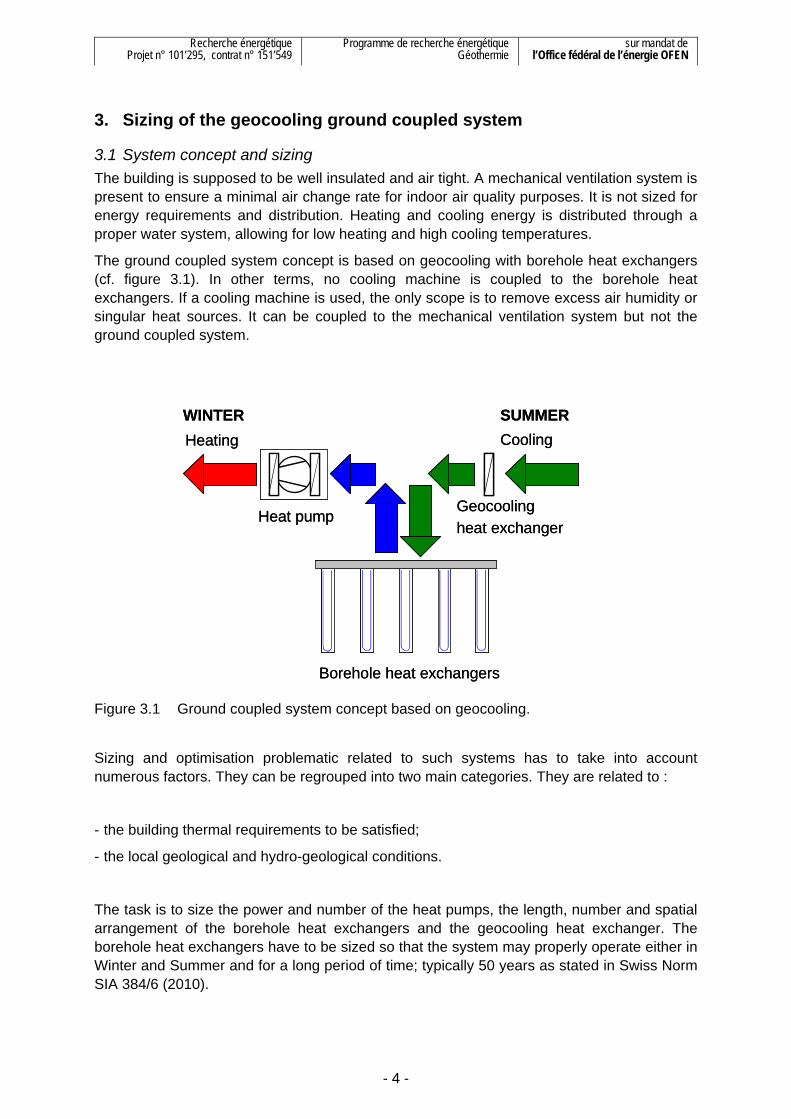
3.1 System concept and sizing The building is supposed to be well insulated and air tight. A mechanical ventilation system is present to ensure a minimal air change rate for indoor air quality purposes. It is not sized for energy requirements and distribution. Heating and cooling energy is distributed through a proper water system, allowing for low heating and high cooling temperatures.
The ground coupled system concept is based on geocooling with borehole heat exchangers (cf. figure 3.1). In other terms, no cooling machine is coupled to the borehole heat exchangers. If a cooling machine is used, the only scope is to remove excess air humidity or singular heat sources. It can be coupled to the mechanical ventilation system but not the ground coupled system.
Figure 3.1 Ground coupled system concept based on geocooling.
Sizing and optimisation problematic related to such systems has to take into account numerous factors. They can be regrouped into two main categories. They are related to :
- the building thermal requirements to be satisfied;
- the local geological and hydro-geological conditions.
The task is to size the power and number of the heat pumps, the length, number and spatial arrangement of the borehole heat exchangers and the geocooling heat exchanger. The borehole heat exchangers have to be sized so that the system may properly operate either in Winter and Summer and for a long period of time; typically 50 years as stated in Swiss Norm SIA 384/6 (2010).
Borehole heat exchangers
Heat pumpGeocoolingheat exchanger
CoolingHeatingWINTER SUMMER
Borehole heat exchangers
Heat pumpGeocoolingheat exchanger
CoolingHeatingWINTER SUMMER

Recherche énergétique Projet n° 101’295, contrat n° 151’549
Programme de recherche énergétique Géothermie
sur mandat de l’Office fédéral de l’énergie OFEN
- 5 -
System sizing is conditioned by the allowed heat carrier fluid temperature variations in the boreholes. Fluid temperature variations depend both on short term system dynamic and long term effects. Short term system dynamic is mainly influenced by the system integration in the building energy concept, heat pump sizing and geocooling temperature levels. Long term effects, for a given borehole configuration and in absence of a significant ground water flow, are in a large extent determined by the ground recharge ratio, i.e. the ratio of the annual injected by the annual extracted heat through the boreholes.
The fluid temperature variations are conditioned by the following limits :
- the minimum return fluid temperature in the boreholes. This temperature limitation has to be fulfilled, normally to prevent shading caused by freezing. If the boreholes are placed under the building, the minimum fluid temperature is fixed to 0°C. In SIA Norm 384/6 (2010), the minimum fluid temperature is fixed to -3°C for boreholes placed outside of the building;
- the maximum return fluid temperature in the boreholes. With geocooling this temperature results from the maximum possible temperature level in the cooling distribution, which should be typically about 20°C or more.
The best system design is obtained when the temperature limitations are fulfilled with the smallest possible borehole length. The main difficulty is to optimise the system while maintaining sufficient margin for taking into account loading conditions or parameters that may deviate from their design values. It is thus important not to have a too tight sizing and know the sensitivity of the main design parameters on the system sizing. In this context, the importance of system simulations does not need to be demonstrated.
3.2 Methodology The initial step is the definition of an office building and location. A reference building geometry is used and the building envelope, building use and building thermal energy distributions are defined together with climatic data for the studied location.
Thermal requirements of the building In a first step the building control parameters are adjusted so that winter and summer thermal comfort are met with a minimum of heating and cooling energy. According to SIA Norm 382/1 (2007), indoor air temperature should remain within 21 – 24.5°C in winter and 22 – 26.5°C in summer. The indoor air temperature may exceed the upper limit up to 100 hours per year. This tolerance is accepted for buildings cooled with the technique of geocooling.
A procedure has been established for the determination of the building control parameters. Those related to winter and summer management of solar protections are adjusted first with the help of one-year simulations of the building alone. The building indoor air temperature is kept between its minimum and maximum design values, set to respectively 20 and 26 °C. A simulated instant heat rate is added or removed from the building spaces if necessary. Then parameters related to technical installation and thermal energy distribution system in the building are adjusted. The one-year simulations performed for this purpose are made with a simple heating and cooling production, to avoid the simulation of the ground coupled system. Heating is provided with a constant design heat rate, corresponding to the design heat rate of the heat pump, and cooling with a design fluid temperature and flow rate, corresponding to geocooling at a given temperature level. It is important not to have an oversized design heat

Recherche énergétique Projet n° 101’295, contrat n° 151’549
Programme de recherche énergétique Géothermie
sur mandat de l’Office fédéral de l’énergie OFEN
- 6 -
rate for heating and a too low design fluid temperature for cooling. These two parameters result primarily from the building design and use. They are key factors for the design and success of a ground coupled system and the possibility of using geocooling for cooling.
Depending on the building design, the building heating and cooling distribution system is not necessarily adequate to ensure a good enough thermal comfort. This is the case for example when an intense but short-duration heat gain has to be removed, requiring both a fast and powerful response of the cooling distribution system. The consequence is a large cooling power capacity and a low cooling temperature, which are both not compatible with a geocooling application. In this study the heating and cooling distribution concept is based on massive emitters, such as concrete ceilings or light-concrete floors. If the cooling distribution concept is not compatible with the building design, the case is not considered and the sizing procedure shown in figure 3.2 is aborted.
Sizing of the borehole heat exchangers In a second step the ground coupled system is simulated. All remaining parameters are defined, from the technical installation to the ground, including number, depth and spacing between the borehole heat exchangers. The best system design is obtained when the heating and geocooling criteria are met with the least borehole length. According to SIA norm 384/6 (2010), the criteria have to be met for a time horizon of 50 years, thus including long term effects in the system design.
The heating criterion is met as long as the inlet fluid temperature in the borehole heat exchangers is larger than the minimum allowed one. As the borehole heat exchangers are supposed to be placed under the building, a minimum fluid temperature of 0°C is fixed.
The geocooling criterion is met as long as the annual tolerance for the maximum indoor air temperature is not exceeded (the air temperature might be larger than 26.5°C for a maximum of 100 hours per year during building use). In other terms, the maximum fluid temperature from the borehole heat exchangers is conditioned by the design fluid temperature for cooling and the geocooling heat exchanger between the cooling distribution and the ground flow circuit.
The best system design is found by successive iterations of 50-years simulations of the whole building and ground coupled system. A schematic view of the followed methodology is shown in figure 3.2.
Variations of the building envelope, building heat distribution systems, climatic data and ground thermal characteristics provide various system designs that allow us to evaluate the geocooling potential of such systems.

Recherche énergétique Projet n° 101’295, contrat n° 151’549
Programme de recherche énergétique Géothermie
sur mandat de l’Office fédéral de l’énergie OFEN
- 7 -
Figure 3.2 Followed methodology for the determination of an optimal system design for a
geocooling ground coupled system.
4. The simulation tool
4.1 The TRNSYS simulation software TRNSYS is a well-known and widely used system simulation programme of transient thermal processes (Klein et al., 2007). Version 16.1 of this programme, chosen to develop a simulation tool of the building and its ground coupled system, provides libraries of subroutines that represent, for example, a multi-zone building, or HVAC components such as a heat pump, water tanks, pumps, pipes, valves, controllers and so on. A TRNSED application has been created and called COOLSIM (Pahud, 2008). COOLSIM is based on PILESIM2 (Pahud, 2007), another TRNSED application dedicated for the simulation of a borehole heat exchanger field, and the TRNSYS TYPE56 model, for the simulation of a building and its heat distribution system.
4.2 Building simulation The building model TYPE56 is configured so that the building envelope, building mass, internal gains, air change rate and solar protections correspond to the desired values. Daily and weekly schedules are defined for building occupation and ventilation. A double-flux
Building envelope, building useHeating and cooling distribution
Climatic data
Building control parameters
Building thermal comfort
satisfied?
1 year simulation
Ground coupled systemGround characteristics
Smallest possible bore length
Heating criterion satisfied?
50 years simulation
Geo--cooling criterion
satisfied?
yes
yes
yesno
no
no
start
end
Building distribution concept
feasible?
stop
no
yes

Recherche énergétique Projet n° 101’295, contrat n° 151’549
Programme de recherche énergétique Géothermie
sur mandat de l’Office fédéral de l’énergie OFEN
- 8 -
ventilation system with a heat recovery unit is simulated during the occupation hours of the building.
The technical installation is either providing heating or cooling to the distribution system of the building. As this latter is supposed to have massive concrete plates between floors, they are used for heat and cold emission. They are so-called “active concrete plates”; the water circulation pipes are imbedded in the middle of the floor concrete plate, by opposition to “floor heating”, where the pipes are imbedded in a light concrete layer over the floor concrete plate. Heat and cold emission occurs primarily through the ceiling, and the large heat capacity of the plates is providing a thermal storage between the technical installation and the heated and cooled spaces. Active concrete plates and floor heating are simulated with the help of fictive thermal zones in the TYPE56 model (Pahud and al., 2008; Pahud et Travaglini, 2002). Four fictive zones were defined for the simulation of the heating and cooling distribution system, in addition to the two thermal zones for the simulation of the building itself. In this way it is possible to simulate and assess the building thermal comfort in one specific room, which could be the most critical one of the building, and still have the dynamic heat balance of the overall building, necessary for the sizing of the ground coupled system.
Only sensible heat or cold are simulated. Humidity and dehumidification of the air are not taken into account. The ventilation system is only designed to guaranty hygienic quality of indoor air. It is assumed that if dehumidification is required, it would be achieved through the ventilation system without increase of the design air flow rate. Latent heat is not taken into account in the building simulation and the simulated technical installation is not coupled to the ventilation system.
4.3 Ground coupled system simulation The borehole heat exchangers are simulated with the non standard TRNSYS duct store component TRNVDSTP, developed at Lund University in Sweden (Hellström, 1989; Pahud and Hellström, 1996), and further developed at the EPFL Lausanne (Pahud et al., 1996). This component is devised for the simulation of thermal processes which involve thermal energy storage in the ground, including a ground heat exchanger that can be a borehole field. It has been used and/or validated in numerous studies; see for example Chuard and al. (1983) or Pahud (1993). TRNVDSTP is at the basis of the TRNSED application PILESIM2 (Pahud, 2007).
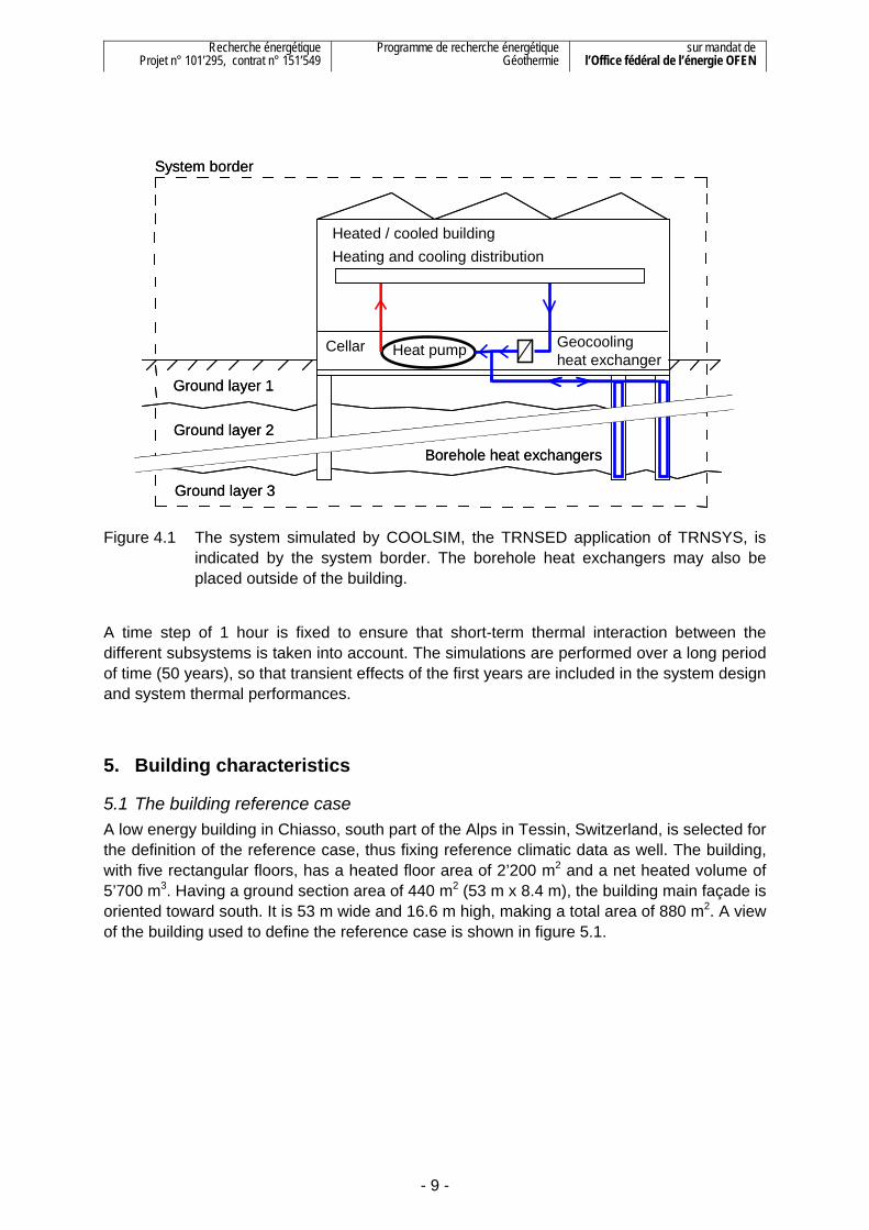
The ground part of PILESIM2 is entirely used and integrated in COOLSIM. The simulated system is indicated by the system border shown in figure 4.1. No domestic hot water is covered by the system.
Recherche énergétique Projet n° 101’295, contrat n° 151’549
Programme de recherche énergétique Géothermie
sur mandat de l’Office fédéral de l’énergie OFEN
- 9 -
Figure 4.1 The system simulated by COOLSIM, the TRNSED application of TRNSYS, is
indicated by the system border. The borehole heat exchangers may also be placed outside of the building.
A time step of 1 hour is fixed to ensure that short-term thermal interaction between the different subsystems is taken into account. The simulations are performed over a long period of time (50 years), so that transient effects of the first years are included in the system design and system thermal performances.
5. Building characteristics
5.1 The building reference case A low energy building in Chiasso, south part of the Alps in Tessin, Switzerland, is selected for the definition of the reference case, thus fixing reference climatic data as well. The building, with five rectangular floors, has a heated floor area of 2’200 m2 and a net heated volume of 5’700 m3. Having a ground section area of 440 m2 (53 m x 8.4 m), the building main façade is oriented toward south. It is 53 m wide and 16.6 m high, making a total area of 880 m2. A view of the building used to define the reference case is shown in figure 5.1.
System border
Ground layer 1
Ground layer 2
Ground layer 3
Borehole heat exchangers
Cellar Heat pump
Heating and cooling distributionHeated / cooled building
Geocoolingheat exchanger
System border
Ground layer 1
Ground layer 2
Ground layer 3
Borehole heat exchangers
Cellar Heat pump
Heating and cooling distributionHeated / cooled building
Geocoolingheat exchanger

Recherche énergétique Projet n° 101’295, contrat n° 151’549
Programme de recherche énergétique Géothermie
sur mandat de l’Office fédéral de l’énergie OFEN
- 10 -
Figure 5.1 Administrative building of the Chiasso-Brogeda’s custom used for the definition
of the reference building.
Opaque parts of the building envelope are well insulated on the outside, keeping the wall thermal mass inside. Outside vertical walls have an inner concrete layer of 18 cm thickness. As the window’s frame is integrated into the opaque walls of the building, the wall U-value is rather large (1 W/(m2K)). The roof, insulated with a layer of 20 cm foam-glass, has a U-value smaller than 0.2 W/(m2K). Due to heating and cooling with the 30 cm thick concrete plates, the ceiling presents large surface of concrete in direct contact with the rooms. The total area of active concrete plates is about 1’900 m2. The building thermal capacity, expressed in terms of internal floor area (1'890 m2), is rather important and corresponds to 150 Wh/(m2K).
The glazing ratio (GR), defined by the windows glazing area over the façade area, is set to 50% for every façade. External solar protections are providing shading on the triple glazing windows (glazing U-value and g-value of respectively 0.7 W/(m2K) and 0.4). When solar protections are completely closed, the overall g-value is reduced to 0.15.
Internal gains from people, lighting and appliances are fixed according to profiles given in the Swiss technical handbook defined for an open space office (SIA, 2006). Expressed in terms of the 1'890 m2 of internal floor area, they reach 26 W/m2 during a working day. On a yearly basis, internal gains correspond to a mean and constant heat emission of 6 W/m2 (1 W/m2 for people, 3.3 W/m2 for lighting and 1.7 W/m2 for appliances).
As the building envelope is air tight, a low but constant infiltration air change rate of 0.1 h-1 is fixed. Mechanical ventilation is operating every day from 8:00 to 18:00 and provides an air
Recherche énergétique Projet n° 101’295, contrat n° 151’549
Programme de recherche énergétique Géothermie
sur mandat de l’Office fédéral de l’énergie OFEN
- 11 -
change rate of 0.5 h-1. Ventilation heat recovery is simulated with an air to air heat exchanger whose efficiency is set to 80%.
The specific transmission and ventilation heat losses of the reference building are assessed to 2.3 kW/K. Together with the internal thermal heat capacity, the time constant of the building is estimated to 120 h.
5.2 Building design variation Various building designs are contemplated relative to the reference one. The glazing ratio (GR 85% instead of 50%), the glazing type (DOUBLE (U-value: 1.4 W/m2K, g-value: 0.6) instead of TRIPLE (U-value: 0.7 W/m2K, g-value: 0.4)), the solar protections (internal (INT) instead of external (EXT)), and the heat and cold distribution system (floor heating (PAV) instead of active concrete plates (TAB)) are analysed. The internal heat capacity of the building designs ranges from 95 to 150 Wh/(m2K), the total specific heat losses from 2.3 to 3.3 kW/K and the time constant from 60 to 120 hours. The characteristics of the external solar protections are such that the overall g-value is 0.15 for both glazing. With internal solar protections the overall g-value results from the solar protection characteristics, and it is calculated to 0.32 for triple glazing and 0.45 for double glazing (see annex 1).
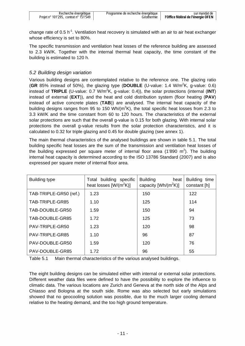
The main thermal characteristics of the analysed buildings are shown in table 5.1. The total building specific heat losses are the sum of the transmission and ventilation heat losses of the building expressed per square meter of internal floor area (1’890 m2). The building internal heat capacity is determined according to the ISO 13786 Standard (2007) and is also expressed per square meter of internal floor area.
Building type Total building specific heat losses [W/(m2K)]
Building heat capacity [Wh/(m2K)]
Building time constant [h]
TAB-TRIPLE-GR50 (ref.) 1.23 150 122
TAB-TRIPLE-GR85 1.10 125 114
TAB-DOUBLE-GR50 1.59 150 94
TAB-DOUBLE-GR85 1.72 125 73
PAV-TRIPLE-GR50 1.23 120 98
PAV-TRIPLE-GR85 1.10 96 87
PAV-DOUBLE-GR50 1.59 120 76
PAV-DOUBLE-GR85 1.72 96 55 Table 5.1 Main thermal characteristics of the various analysed buildings.
The eight building designs can be simulated either with internal or external solar protections. Different weather data files were defined to have the possibility to explore the influence to climatic data. The various locations are Zurich and Geneva at the north side of the Alps and Chiasso and Bologna at the south side. Rome was also selected but early simulations showed that no geocooling solution was possible, due to the much larger cooling demand relative to the heating demand, and the too high ground temperature.
Recherche énergétique Projet n° 101’295, contrat n° 151’549
Programme de recherche énergétique Géothermie
sur mandat de l’Office fédéral de l’énergie OFEN
- 12 -
6. Building thermal performances and comfort
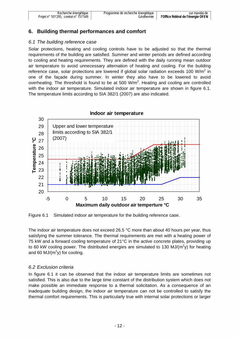
6.1 The building reference case Solar protections, heating and cooling controls have to be adjusted so that the thermal requirements of the building are satisfied. Summer and winter periods are defined according to cooling and heating requirements. They are defined with the daily running mean outdoor air temperature to avoid unnecessary alternation of heating and cooling. For the building reference case, solar protections are lowered if global solar radiation exceeds 100 W/m2 in one of the façade during summer. In winter they also have to be lowered to avoid overheating. The threshold is found to be at 500 W/m2. Heating and cooling are controlled with the indoor air temperature. Simulated indoor air temperature are shown in figure 6.1. The temperature limits according to SIA 382/1 (2007) are also indicated.
Indoor air temperature
2021222324252627282930
-5 0 5 10 15 20 25 30 35Maximum daily outdoor air temperture °C
Tem
pera
ture
°C
Upper and lower temperature limits according to SIA 382/1 (2007)
Figure 6.1 Simulated indoor air temperature for the building reference case.
The indoor air temperature does not exceed 26.5 °C more than about 40 hours per year, thus satisfying the summer tolerance. The thermal requirements are met with a heating power of 75 kW and a forward cooling temperature of 21°C in the active concrete plates, providing up to 60 kW cooling power. The distributed energies are simulated to 130 MJ/(m2y) for heating and 60 MJ/(m2y) for cooling.
6.2 Exclusion criteria In figure 6.1 it can be observed that the indoor air temperature limits are sometimes not satisfied. This is also due to the large time constant of the distribution system which does not make possible an immediate response to a thermal solicitation. As a consequence of an inadequate building design, the indoor air temperature can not be controlled to satisfy the thermal comfort requirements. This is particularly true with internal solar protections or larger

Recherche énergétique Projet n° 101’295, contrat n° 151’549
Programme de recherche énergétique Géothermie
sur mandat de l’Office fédéral de l’énergie OFEN
- 13 -
glazing areas. Floor heating also presents more difficulties than active concrete plates to keep indoor air temperature within minimum and maximum limits.
Building designs that present difficulties for the control of indoor climate normally require larger heating and cooling powers, which means a lower forward fluid temperature for cooling. Large power and low temperature for cooling are not compatible with geocooling. This study has clearly highlighted that only low energy buildings that integrate passive climate control such as efficient external solar protections and active concrete plates can take the full benefice of the geocooling potential.
Most of the heating and cooling energy has to be distributed through the heat distribution system and not the ventilation system. This is the reason why indoor air temperature comfort requirements have to be satisfied without air conditioning in the simulation model. If this is not possible a geocooling solution has no sense and the first step of the procedure shown in figure 3.2 is aborted.
Exclusion criteria were established to easily identify problematic building cases. The first criterion is of course linked to the summer tolerance comfort:
- if Tindoor air > 26.5°C for more that 50 hours per year, then the case is eliminated. Half of the SIA norm tolerance is adopted, in order to keep some margin when the geocooling system is sized.
When the building control parameters are set, a procedure is followed to fix them one after one. The building is first simulated without the heat distribution system, allowing to determine the annual heating and cooling demand of the building. At the end of the procedure, the heat distribution system is simulated and the annual distributed energy for heating and cooling is simulated. Due to the imperfect distribution system and simple system control, the distributed energy is greater than the energy demand. The second exclusion criterion is related to the distributed to the demanded energy ratio:
- if the distributed energy is greater than 3 times the energy demand, either for heating or cooling, then the case is eliminated.
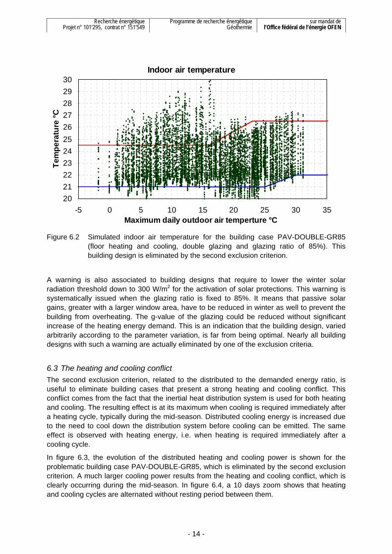
In figure 6.2, simulated indoor air temperature are shown for the building case PAV-DOUBLE-GR85. This case is eliminated by the second exclusion criterion, as the ratio distributed over demanded annual energy is about 4 for both heating and cooling. It can be observed that indoor air temperatures are not always enclosed inside the temperature limits according to SIA 382/1 (2007), in particular due to overheating in winter. The difficulty to maintain a satisfactory thermal comfort confirms the exclusion of this building design by the second criterion.
Recherche énergétique Projet n° 101’295, contrat n° 151’549
Programme de recherche énergétique Géothermie
sur mandat de l’Office fédéral de l’énergie OFEN
- 14 -
Indoor air temperature
2021222324252627282930
-5 0 5 10 15 20 25 30 35Maximum daily outdoor air temperture °C
Tem
pera
ture
°C
Figure 6.2 Simulated indoor air temperature for the building case PAV-DOUBLE-GR85
(floor heating and cooling, double glazing and glazing ratio of 85%). This building design is eliminated by the second exclusion criterion.
A warning is also associated to building designs that require to lower the winter solar radiation threshold down to 300 W/m2 for the activation of solar protections. This warning is systematically issued when the glazing ratio is fixed to 85%. It means that passive solar gains, greater with a larger window area, have to be reduced in winter as well to prevent the building from overheating. The g-value of the glazing could be reduced without significant increase of the heating energy demand. This is an indication that the building design, varied arbitrarily according to the parameter variation, is far from being optimal. Nearly all building designs with such a warning are actually eliminated by one of the exclusion criteria.
6.3 The heating and cooling conflict The second exclusion criterion, related to the distributed to the demanded energy ratio, is useful to eliminate building cases that present a strong heating and cooling conflict. This conflict comes from the fact that the inertial heat distribution system is used for both heating and cooling. The resulting effect is at its maximum when cooling is required immediately after a heating cycle, typically during the mid-season. Distributed cooling energy is increased due to the need to cool down the distribution system before cooling can be emitted. The same effect is observed with heating energy, i.e. when heating is required immediately after a cooling cycle.
In figure 6.3, the evolution of the distributed heating and cooling power is shown for the problematic building case PAV-DOUBLE-GR85, which is eliminated by the second exclusion criterion. A much larger cooling power results from the heating and cooling conflict, which is clearly occurring during the mid-season. In figure 6.4, a 10 days zoom shows that heating and cooling cycles are alternated without resting period between them.

Recherche énergétique Projet n° 101’295, contrat n° 151’549
Programme de recherche énergétique Géothermie
sur mandat de l’Office fédéral de l’énergie OFEN
- 15 -
Heating and cooling energy demands
0
50
100
150
200
250
300
350
0.00 0.25 0.50 0.75 1.00time (year)
Ther
mal
pow
er k
W
Heating demandCooling demand
Figure 6.3 Simulated distributed heating and cooling power in the distribution system for
the building case PAV-DOUBLE-GR85 (floor heating and cooling, double glazing and glazing ratio of 85%). The heating and cooling conflict is observed during the mid-season and results in very large and instant cooling powers.
Heating and cooling energy demands
0
50
100
150
200
250
300
350
0.250 0.255 0.261 0.266 0.272 0.277time (year)
Ther
mal
pow
er k
W
Heating demandCooling demand
Figure 6.4 Ten-days zoom during the mid-season of the simulated distributed heating and
cooling power in the distribution system for the building case PAV-DOUBLE-GR85 (floor heating and cooling, double glazing and glazing ratio of 85%).
Recherche énergétique Projet n° 101’295, contrat n° 151’549
Programme de recherche énergétique Géothermie
sur mandat de l’Office fédéral de l’énergie OFEN
- 16 -
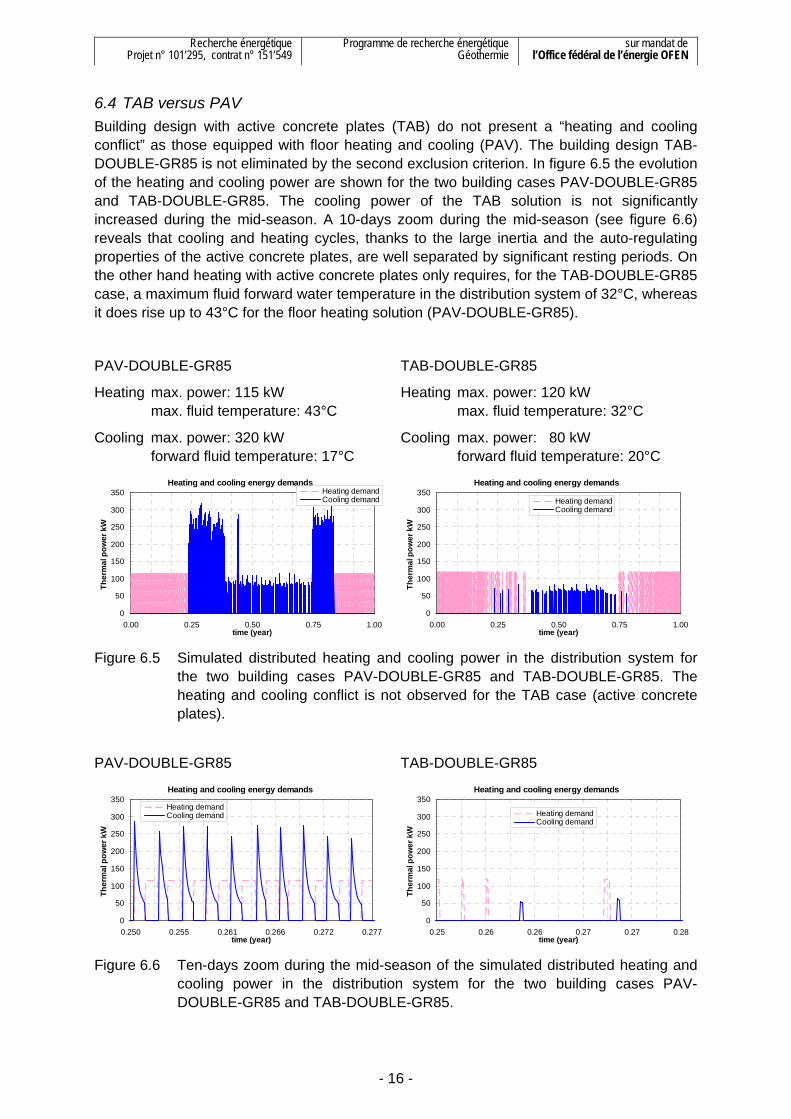
6.4 TAB versus PAV Building design with active concrete plates (TAB) do not present a “heating and cooling conflict” as those equipped with floor heating and cooling (PAV). The building design TAB-DOUBLE-GR85 is not eliminated by the second exclusion criterion. In figure 6.5 the evolution of the heating and cooling power are shown for the two building cases PAV-DOUBLE-GR85 and TAB-DOUBLE-GR85. The cooling power of the TAB solution is not significantly increased during the mid-season. A 10-days zoom during the mid-season (see figure 6.6) reveals that cooling and heating cycles, thanks to the large inertia and the auto-regulating properties of the active concrete plates, are well separated by significant resting periods. On the other hand heating with active concrete plates only requires, for the TAB-DOUBLE-GR85 case, a maximum fluid forward water temperature in the distribution system of 32°C, whereas it does rise up to 43°C for the floor heating solution (PAV-DOUBLE-GR85).
PAV-DOUBLE-GR85
Heating max. power: 115 kW max. fluid temperature: 43°C
Cooling max. power: 320 kW forward fluid temperature: 17°C
TAB-DOUBLE-GR85
Heating max. power: 120 kW max. fluid temperature: 32°C
Cooling max. power: 80 kW forward fluid temperature: 20°C
Heating and cooling energy demands
0
50
100
150
200
250
300
350
0.00 0.25 0.50 0.75 1.00time (year)
Ther
mal
pow
er k
W
Heating demandCooling demand
Heating and cooling energy demands
0
50
100
150
200
250
300
350
0.00 0.25 0.50 0.75 1.00time (year)
Ther
mal
pow
er k
W
Heating demandCooling demand
Figure 6.5 Simulated distributed heating and cooling power in the distribution system for the two building cases PAV-DOUBLE-GR85 and TAB-DOUBLE-GR85. The heating and cooling conflict is not observed for the TAB case (active concrete plates).
PAV-DOUBLE-GR85 TAB-DOUBLE-GR85
Heating and cooling energy demands
0
50
100
150
200
250
300
350
0.250 0.255 0.261 0.266 0.272 0.277time (year)
Ther
mal
pow
er k
W
Heating demandCooling demand
Heating and cooling energy demands
0
50
100
150
200
250
300
350
0.25 0.26 0.26 0.27 0.27 0.28time (year)
Ther
mal
pow
er k
W
Heating demandCooling demand
Figure 6.6 Ten-days zoom during the mid-season of the simulated distributed heating and cooling power in the distribution system for the two building cases PAV-DOUBLE-GR85 and TAB-DOUBLE-GR85.

Recherche énergétique Projet n° 101’295, contrat n° 151’549
Programme de recherche énergétique Géothermie
sur mandat de l’Office fédéral de l’énergie OFEN
- 17 -
Even for cases that where not eliminated, the PAV solution (floor heating and cooling) exhibits symptoms of the “heating and cooling conflict”. This is illustrated with figures 6.7 and 6.8, that presents the two cases PAV-DOUBLE-GR50 and TAB-DOUBLE-GR50, both kept for geocooling sizing.
PAV-DOUBLE-GR50
Heating max. power: 100 kW max. fluid temperature: 38°C
Cooling max. power: 135 kW forward fluid temperature: 20°C
TAB-DOUBLE-GR50
Heating max. power: 100 kW max. fluid temperature: 31°C
Cooling max. power: 50 kW forward fluid temperature: 22°C
Heating and cooling energy demands
0
20
40
60
80
100
120
140
0.00 0.25 0.50 0.75 1.00time (year)
Ther
mal
pow
er k
W
Heating demandCooling demand
Heating and cooling energy demands
0
20
40
60
80
100
120
140
0.00 0.25 0.50 0.75 1.00time (year)
Ther
mal
pow
er k
W
Heating demandCooling demand
Figure 6.7 Simulated distributed heating and cooling power in the distribution system for the two building cases PAV-DOUBLE-GR50 and TAB-DOUBLE-GR50. The heating and cooling conflict is still observed for the PAV case (floor heating and cooling), although it has been kept for geocooling sizing.
PAV-DOUBLE-GR50 TAB-DOUBLE-GR50
Heating and cooling energy demands
0
20
40
60
80
100
120
140
0.25 0.26 0.26 0.27 0.27 0.28time (year)
Ther
mal
pow
er k
W
Heating demandCooling demand
Heating and cooling energy demands
0
20
40
60
80
100
120
140
0.25 0.26 0.26 0.27 0.27 0.28time (year)
Ther
mal
pow
er k
W
Heating demandCooling demand
Figure 6.8 Ten-days zoom during the mid-season of the simulated distributed heating and cooling power in the distribution system for the two building cases PAV-DOUBLE-GR50 and TAB-DOUBLE-GR50.
The TAB solution appears to be better adequate for the chosen heat distribution concept, which uses the same distribution flow circuit for both heating and cooling. It does better separates the heating requirements from the cooling ones. Unlike the PAV solution, the TAB solution does not show obvious indications of the heating and cooling conflict. It can also be noticed that relatively to a PAV solution, a TAB solution allows lower heating and higher cooling temperatures, which plays in favour of a geocooling solution and a higher system

Recherche énergétique Projet n° 101’295, contrat n° 151’549
Programme de recherche énergétique Géothermie
sur mandat de l’Office fédéral de l’énergie OFEN
- 18 -
efficiency. If a TAB solution can provide a satisfactory thermal comfort, then the chances that a geocooling solution is feasible are great.
6.5 Building designs for geocooling For all the simulated locations, the building designs with a glazing ratio of 85% were eliminated. An acceptable solution would only be possible if the overall g-value of the windows and solar protections is further reduced from 0.15 down to 0.08, as requested by the SIA 382/1 Swiss norm (2007). Only the TAB solution with TRIPLE glazing was accepted for a GR of 85%, although the case presents obvious difficulties to maintain the indoor air temperature within thermal comfort limits.
The building designs with indoor solar protections were also eliminated. Only the TAB solution with TRIPLE glazing and a GR of 50% was not rejected, although difficulties to maintain the indoor air temperature within thermal comfort limits were also observed.
It was also observed that the use of TRIPLE glazing instead of DOUBLE glazing resulted in less annual heating energy and more annual cooling energy. As a result, the ground recharge ratio is increased.

Recherche énergétique Projet n° 101’295, contrat n° 151’549
Programme de recherche énergétique Géothermie
sur mandat de l’Office fédéral de l’énergie OFEN
- 19 -
7. Heating and geocooling sizing keys
7.1 Introduction The reference building with the reference location is chosen for the simulation analysis (TAB-TRIPLE-GR50 in Chiasso, see chapter 5). In order to explore the results in function of the ground recharge ratio, the internal gains are scaled from 60% to 140%. Eleven cases are simulated, making the ground recharge ratio vary from 25 to 100%. The heating and cooling maximum thermal powers are shown in table 7.1 and 7.2, and the annual distributed energies in table 7.3.
TAB-TRIPLE-GR50
Location: Chiasso
Maximum heating power demand
Nominal or design installed heat pump
power (B0W35)
Nominal heat extraction rate
(COP: 4 at B0W35)
Internal heat gains magnitude [kW] [kW] [kW]
60% 76 77 57.8
70% 76 75 56.3
80% 75 75 56.3
90% 75 75 56.3
95% 74 75 56.3
100% 74 75 56.3
105% 73 75 56.3
110% 73 75 56.3
120% 73 75 56.3
130% 74 75 56.3
140% 73 75 56.3 Table 7.1 Maximum and design thermal powers for heating in function of the magnitude of
the internal heat gains in the reference building design. The installed nominal heating power is fixed to about the maximum heating power demand of the building. It corresponds to the heat pump heating power at B0W35 operating conditions.
The maximum heating power demand is obtained by simulating the building without the heat distribution system, i.e. by setting the minimum indoor air temperature of the building to 20°C. The building is simulated for its normal use, including internal heat gains and passive solar gains, and the maximum heat power demand results from the hourly heat balance of the building, so that the indoor air temperature never drops under the minimum set point value of 20°C. The maximum heat power of 75 kW, expressed in relation to the reference heated floor area of 2’200 m2, corresponds to 34 W/m2. This is a typical value for a building designed to fulfil the low energy Minergie® standard from 2005.

Recherche énergétique Projet n° 101’295, contrat n° 151’549
Programme de recherche énergétique Géothermie
sur mandat de l’Office fédéral de l’énergie OFEN
- 20 -
The maximum heating power demand is slightly sensitive to the magnitude of the internal heat gains. The nominal or design installed heating power is fixed to a value close to the maximum heating power demand. It corresponds to the thermal power output of the heat pump operating at B0W35 conditions.
TAB-TRIPLE-GR50
Location: Chiasso
Maximum cooling power demand
Design forward water temperature in
cooling distribution
Maximum effective distributed cooling
power
Internal heat gains magnitude [kW] [°C] [kW]
60% 54 22 56
70% 59 22 46
80% 64 21 73
90% 69 21 66
95% 71 21 66
100% 74 21 65
105% 76 20 83
110% 79 20 83
120% 84 20 83
130% 89 19 98
140% 94 19 99 Table 7.2 Maximum thermal powers and design fluid temperature for cooling in function of
the magnitude of the internal heat gains in the reference building design. The maximum effective distributed cooling power also depends on the required design forward fluid temperature necessary to maintain a satisfactory thermal comfort.
The maximum cooling power demand is obtained by simulating the building without the cooling distribution system, i.e. by setting the maximum indoor air temperature of the building to 26°C. The building is simulated for its normal use, including internal heat gains and passive solar gains, and the maximum cooling power demand results from the hourly heat balance of the building, so that the indoor air temperature never exceeds the maximum set point value of 26°C. The maximum cooling power demand is strongly dependent on the magnitude of the internal heat gains. Expressed in relation to the reference heated floor area of 2’200 m2, the maximum cooling power varies from 21 to 45 W/m2. These values are relatively low and result from both a building designed to fulfil the low energy Minergie® standard and the use of active concrete plates (TABS) for cooling.
The maximum effective distributed cooling power is not only sensitive to the magnitude of the internal heat gains, but also to the design forward fluid temperature in the cooling distribution. This latter is found with the help of simulations: it corresponds to the maximum possible
Recherche énergétique Projet n° 101’295, contrat n° 151’549
Programme de recherche énergétique Géothermie
sur mandat de l’Office fédéral de l’énergie OFEN
- 21 -
design fluid temperature that still keep thermal comfort parameters within SIA Norm 382/1 (2007) requirements.
TAB-TRIPLE-GR50
Location: Chiasso
Annual distributed heating energy
Annual distributed cooling energy, in % of the heating one
Ground recharge ratio
Internal heat gains magnitude [MWh/y] [%] [%]
60% 94 21 25
70% 88 28 33
80% 89 31 37
90% 83 41 50
95% 81 44 54
100% 79 48 59
105% 77 56 66
110% 77 58 70
120% 73 68 81
130% 75 77 91
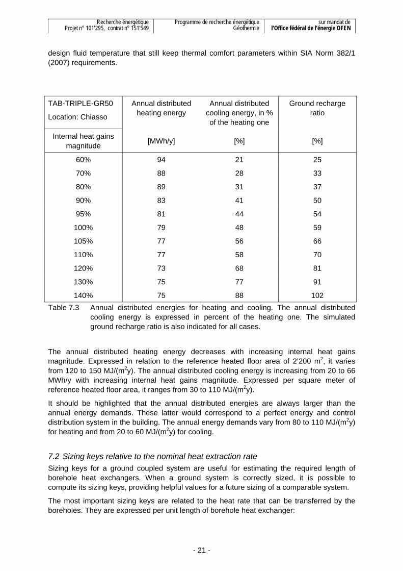
140% 75 88 102 Table 7.3 Annual distributed energies for heating and cooling. The annual distributed
cooling energy is expressed in percent of the heating one. The simulated ground recharge ratio is also indicated for all cases.
The annual distributed heating energy decreases with increasing internal heat gains magnitude. Expressed in relation to the reference heated floor area of 2’200 m2, it varies from 120 to 150 MJ/(m2y). The annual distributed cooling energy is increasing from 20 to 66 MWh/y with increasing internal heat gains magnitude. Expressed per square meter of reference heated floor area, it ranges from 30 to 110 MJ/(m2y).
It should be highlighted that the annual distributed energies are always larger than the annual energy demands. These latter would correspond to a perfect energy and control distribution system in the building. The annual energy demands vary from 80 to 110 MJ/(m2y) for heating and from 20 to 60 MJ/(m2y) for cooling.
7.2 Sizing keys relative to the nominal heat extraction rate Sizing keys for a ground coupled system are useful for estimating the required length of borehole heat exchangers. When a ground system is correctly sized, it is possible to compute its sizing keys, providing helpful values for a future sizing of a comparable system.
The most important sizing keys are related to the heat rate that can be transferred by the boreholes. They are expressed per unit length of borehole heat exchanger:

Recherche énergétique Projet n° 101’295, contrat n° 151’549
Programme de recherche énergétique Géothermie
sur mandat de l’Office fédéral de l’énergie OFEN
- 22 -
- qe specific heat extraction rate (or heating sizing key) [W/m]
- qi specific heat injection rate (or geocooling sizing key) [W/m]
Secondary but not least important sizing keys are related to the storage effect of the borehole heat exchangers. The ground recharge ratio, i.e. the fraction of the annual extracted energy that is injected back into the ground during an annual cycle, has a strong influence on the specific heat rate key values.
- Qe specific annual heat extraction energy [kWh/m/y]
- Qi specific annual heat injection energy [kWh/m/y]
- ηg = Qi/Qe ground recharge ratio [-]
In a first step, the heating and geocooling sizing keys are both determined on the basis of the nominal heat extraction rate of the heat pump (see table 7.1) and the required borehole length to meet the heating or the geocooling criterion. The geocooling sizing key, calculated in this way, does not provide a specific heat injection rate, but corresponds to a sizing number that can be directly compared to the heating one. They are shown in the same graphic in figure 7.1 and they are represented in function of the ground recharge ratio ηg. The results are obtained for 100m deep boreholes spaced with 8m, equipped with standard double-U pipe installation and bentonite-cement filling material. The ground thermal conductivity is fixed to an average value of 2 W/(mK). Initial ground temperature is 12°C near the surface with a mean geothermal temperature gradient of 25 K/km.
0
10
20
30
40
50
60
70
0 20 40 60 80 100 120Ground recharge ratio [%]
Nom
inal
hea
t ext
ract
ion
rate
per
bo
reho
le le
ngth
[W/m
]
0
10
20
30
40
50
60
70
Ground thermal conductivity 2.0 [W/(mK)]
Geocooling criterion
Heating criterion
Figure 7.1 Heating and geocooling sizing keys expressed in relation to the nominal heat
extraction rate and represented in function of the ground recharge ratio.

Recherche énergétique Projet n° 101’295, contrat n° 151’549
Programme de recherche énergétique Géothermie
sur mandat de l’Office fédéral de l’énergie OFEN
- 23 -
In this case, an optimal borehole length is obtained for a ground recharge ratio of 50 – 60%. As expected the heating criterion dominates and conditions the borehole sizing at small values of the ground recharge ratio, whereas it is the geocooling criterion that dominates at large ground recharge ratio. It can be observed that the required borehole length is becoming extremely important for small ground recharge ratio (scarce recharge) and for a complete recharge of the ground.
In figure 7.1, the specific heat extraction rate is varying regularly in relation to the ground ratio, confirming the natural choice of the nominal heat extraction rate as a representative thermal power to be used to establish the heating sizing key. This is not the case with the geocooling sizing key, which exhibits variations by successive steps. These steps can be correlated to the steps of the maximum effective distributed cooling powers. The total borehole length required for cooling has an inversely proportional behaviour relative to the maximum distributed cooling powers.
40
50
60
70
80
90
100
40 50 60 70 80 90 100Maximum cooling power demand of the building [kW]
Max
imum
effe
ctiv
e di
strib
uted
coo
ling
pow
er [k
W]
40
50
60
70
80
90
100Tset-cool 19°C; Tset-air 24.5°C; ΔT 5.5K
Tc 20°C; Ta 24.5°C; ΔT 4.5K
Tc 21°C; Ta 24.5°C; ΔT 3.5K
Tc 21°C; Ta 25.0°C; ΔT 4.0K
Tc 22°C; Ta 24.5°C; ΔT 2.5K
Tc 22°C; Ta 25.0°C; ΔT 3.0K
Figure 7.2 Maximum effective distributed cooling power shown in relation to the maximum
cooling power demand of the building. The design forward water temperature in the cooling distribution (Tset-cool or Tc) and the indoor set-point air temperature (Tset-air or Ta) have a significant influence on the maximum effective distributed cooling power.
The stepwise behaviour of the maximum effective distributed cooling power is shown in figure 7.2. It can be observed how it is conditioned by the temperature difference between indoor set-point temperature (Ta) and design forward water temperature in the cooling distribution (Tc). These two temperatures are fixed when the building control parameters are adjusted according to the first step of the methodology shown in figure 3.2 to meet thermal comfort requirements. As these temperatures are varied stepwise, the resulting distributed

Recherche énergétique Projet n° 101’295, contrat n° 151’549
Programme de recherche énergétique Géothermie
sur mandat de l’Office fédéral de l’énergie OFEN
- 24 -
cooling power is also varying in a stepwise manner, although the maximum cooling power demand is increasing linearly with internal heat gain increase.
The lower the design forward water temperature (Tc) the greater becomes the distributed cooling power. The effect on the total borehole length is twice toward a larger one, due to a larger cooling power to be met and a smaller available temperature difference between the ground and the water in the cooling distribution (Tc). This is why the variation of the geocooling sizing key is so large in figure 7.1. As the nominal heat extraction rate is quasi the same for all the cases shown in figure 7.1, the variation of the geocooling sizing key is a measure of the total borehole length variation. It can be observed that the bore variation is much greater for geocooling than for heating.
This confirms the necessity to design buildings together with cooling distribution systems that makes possible a high cooling temperature and a large thermal capacity to limit the peak cooling loads to be evacuated.
7.3 Definition of heating and geocooling sizing keys For the heating case, a relevant thermal power is the nominal heat extraction rate of the heat pump. This is a logical choice as the design thermal power of the installed heat pump is fixed to match the maximum heat power demand of the building. In figure 7.3, the heating sizing key is computed in relation to both the nominal heat extraction rate corresponding to the installed heat pump and the nominal heat extraction rate that would correspond to the maximum heat power demand of the building. No significant difference can be observed.
0
10
20
30
40
50
60
70
0 20 40 60 80 100 120Ground recharge ratio [%]
Hea
t ext
ract
ion
rate
per
bor
ehol
e le
ngth
[W
/m]
0
10
20
30
40
50
60
70
Ground thermal conductivity 2.0 [W/(mK)]
Nominal heat extraction rate corresponding to the installed heat pump (nominal COP: 4)
Heating criterion
Nominal heat extraction rate (COP: 4) corresponding to the maximum heat power demand of the building
Figure 7.3 Heating sizing keys expressed in relation to both the nominal heat extraction
rate of the installed heat pump and the heat extraction rate that would result from the maximum heat power demand.

Recherche énergétique Projet n° 101’295, contrat n° 151’549
Programme de recherche énergétique Géothermie
sur mandat de l’Office fédéral de l’énergie OFEN
- 25 -
The decrease of the heating sizing key with a smaller ground recharge ratio is a consequence of the long term effects, taken into account in the design up to a time horizon of 50 years. Long term effects are without influence for a ground recharge ratio of 100%, and the heating sizing key, calculated to about 40 W/m, would correspond to a single borehole heat exchanger. This value is low as the minimum tolerated return fluid temperature in the borehole is fixed to 0°C instead of -3°C, as it would be the case if the boreholes were located outside of the building. With -3°C the heating sizing key would be slightly above 50 W/m.
The specific annual heat extraction energy lies between 30 [kWh/m/y] (case with the smaller ground recharge ratio) and 40 [kWh/m/y] (case with the greater ground recharge ratio).
For the cooling case, a relevant thermal power is the maximum effective distributed cooling power. In figure 7.4, the geocooling sizing key is computed in relation to both the maximum effective distributed cooling power and the maximum cooling power demand of the building. The maximum effective distributed cooling power appears to be more convenient. The geocooling sizing key do not show a step-wise variation. However the dispersion of the values is larger than for the heating case, most likely due to a much stronger interaction of the ground coupled system with the building.
0
10
20
30
40
50
60
70
0 20 40 60 80 100 120Ground recharge ratio [%]
Max
imum
coo
ling
pow
er p
er b
oreh
ole
leng
th [W
/m]
0
10
20
30
40
50
60
70
Ground thermal conductivity 2.0 [W/(mK)]
Geocooling criterion
Maximum effective distributed cooling powerMaximum cooling power demand of the building
Figure 7.4 Geocooling sizing keys expressed in relation to both the maximum effective
distributed cooling power and the maximum cooling power demand of the building.
The long term effects are favourable to geocooling, as long as the ground recharge ratio is smaller than 100%, which tends to slightly decrease the ground temperature in the ground volume enclosed by the boreholes. However the increase of the geocooling sizing key with a smaller ground recharge ratio is not a consequence of the long term effects, as cooling has to be met the first operation year as well. The increase of the geocooling sizing key is

Recherche énergétique Projet n° 101’295, contrat n° 151’549
Programme de recherche énergétique Géothermie
sur mandat de l’Office fédéral de l’énergie OFEN
- 26 -
primarily due to the design forward water temperature in the cooling distribution, which can be increased with a decreasing ground recharge ratio, thanks to a smaller cooling load. The specific annual heat injection energy lies between 10 and 30 [kWh/m/y].
The heating and geocooling sizing keys are defined as follow:
- qe nominal heat extraction rate of the heat pump per length unit of borehole heat exchanger [W/m]
- qi maximum distributed cooling power per length unit of borehole heat exchanger [W/m]
The heating and geocooling sizing keys are significantly sensitive to:
- ηg the ground recharge ratio [-]
7.4 Sensitivity of the sizing keys to some significant design parameters The sensitivity of the sizing keys to some design parameters is assessed and shown in figures 7.5 to 7.9. The examined parameters are:
- the ground thermal conductivity (figure 7.5);
- the borehole spacing (figure 7.6);
- the borehole depth (figure 7.7);
- the initial ground temperature (figure 7.8);
- and the heat transfer capacity of the geocooling heat exchanger (figure 7.9).
When a parameter is varied, the others are fixed to their reference value. They are:
- reference ground thermal conductivity: 2 W/(mK);
- reference borehole spacing: 8 m;
- reference borehole depth: 100 m;
- reference initial ground temperature near the surface: 12 °C;
- and the reference heat transfer capacity of the geocooling heat exchanger: 30 kW/K.
As expected a greater ground thermal conductivity is better for both heating and geocooling sizing keys. The borehole spacing has no noticeable influence on the geocooling sizing keys. Its effect on the heating sizing keys is only perceptible at low ground recharge ratio, when long term effects are becoming more important. A warmer ground or deeper boreholes are favourable to the heating sizing keys but not to the geocooling ones. Depending on the building design and ground temperature, an optimal borehole depth might be found.
The heat transfer capacity of the geocooling heat exchanger only influences the geocooling sizing keys. An undersized geocooling heat exchanger has a negative effect on the required borehole length for geocooling and significantly increases it.
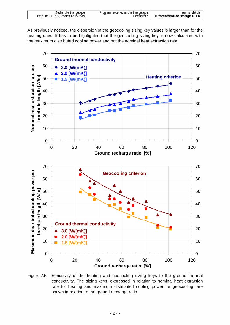
Recherche énergétique Projet n° 101’295, contrat n° 151’549
Programme de recherche énergétique Géothermie
sur mandat de l’Office fédéral de l’énergie OFEN
- 27 -
As previously noticed, the dispersion of the geocooling sizing key values is larger than for the heating ones. It has to be highlighted that the geocooling sizing key is now calculated with the maximum distributed cooling power and not the nominal heat extraction rate.
0
10
20
30
40
50
60
70
0 20 40 60 80 100 120Ground recharge ratio [%]
Nom
inal
hea
t ext
ract
ion
rate
per
bo
reho
le le
ngth
[W/m
]
0
10
20
30
40
50
60
70Ground thermal conductivity
Heating criterion
3.0 [W/(mK)]2.0 [W/(mK)]1.5 [W/(mK)]
0
10
20
30
40
50
60
70
0 20 40 60 80 100 120Ground recharge ratio [%]
Max
imum
dis
tribu
ted
cool
ing
pow
er p
er
bore
hole
leng
th [W
/m]
0
10
20
30
40
50
60
70
Ground thermal conductivity
Geocooling criterion
3.0 [W/(mK)]2.0 [W/(mK)]1.5 [W/(mK)]
Figure 7.5 Sensitivity of the heating and geocooling sizing keys to the ground thermal
conductivity. The sizing keys, expressed in relation to nominal heat extraction rate for heating and maximum distributed cooling power for geocooling, are shown in relation to the ground recharge ratio.

Recherche énergétique Projet n° 101’295, contrat n° 151’549
Programme de recherche énergétique Géothermie
sur mandat de l’Office fédéral de l’énergie OFEN
- 28 -
0
10
20
30
40
50
60
70
0 20 40 60 80 100 120Ground recharge ratio [%]
Nom
inal
hea
t ext
ract
ion
rate
per
bo
reho
le le
ngth
[W/m
]
0
10
20
30
40
50
60
70
Ground thermal conductivity 2.0 [W/(mK)]
Heating criterion
Borehole spacing10 [m] 8 [m] 6 [m]
0
10
20
30
40
50
60
70
0 20 40 60 80 100 120Ground recharge ratio [%]
Max
imum
dis
tribu
ted
cool
ing
pow
er p
er
bore
hole
leng
th [W
/m]
0
10
20
30
40
50
60
70
Ground thermal conductivity 2.0 [W/(mK)]
Geocooling criterion
Borehole spacing10 [m] 8 [m] 6 [m]
Figure 7.6 Sensitivity of the heating and geocooling sizing keys to the borehole spacing.
The sizing keys, expressed in relation to nominal heat extraction rate for heating and maximum distributed cooling power for geocooling, are shown in relation to the ground recharge ratio.
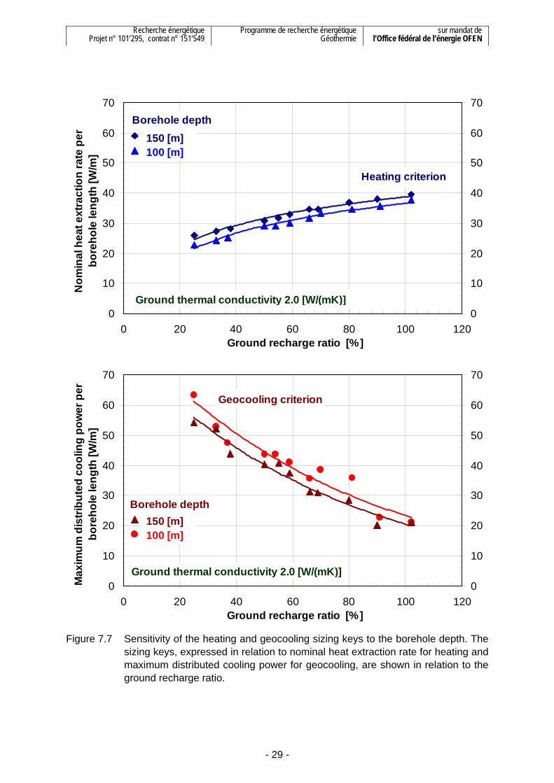
Recherche énergétique Projet n° 101’295, contrat n° 151’549
Programme de recherche énergétique Géothermie
sur mandat de l’Office fédéral de l’énergie OFEN
- 29 -
0
10
20
30
40
50
60
70
0 20 40 60 80 100 120Ground recharge ratio [%]
Nom
inal
hea
t ext
ract
ion
rate
per
bo
reho
le le
ngth
[W/m
]
0
10
20
30
40
50
60
70
Ground thermal conductivity 2.0 [W/(mK)]
Borehole depth
Heating criterion
150 [m]100 [m]
0
10
20
30
40
50
60
70
0 20 40 60 80 100 120Ground recharge ratio [%]
Max
imum
dis
tribu
ted
cool
ing
pow
er p
er
bore
hole
leng
th [W
/m]
0
10
20
30
40
50
60
70
Ground thermal conductivity 2.0 [W/(mK)]
Geocooling criterion
Borehole depth150 [m]100 [m]
Figure 7.7 Sensitivity of the heating and geocooling sizing keys to the borehole depth. The
sizing keys, expressed in relation to nominal heat extraction rate for heating and maximum distributed cooling power for geocooling, are shown in relation to the ground recharge ratio.
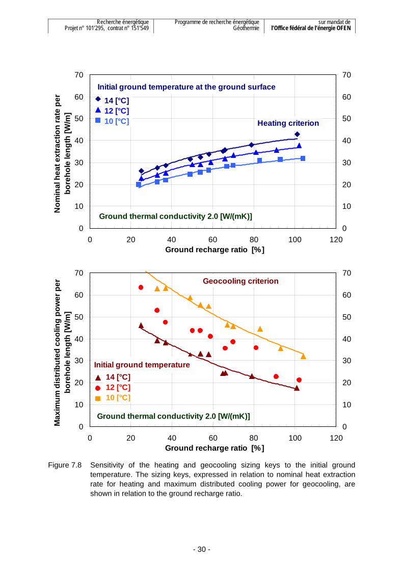
Recherche énergétique Projet n° 101’295, contrat n° 151’549
Programme de recherche énergétique Géothermie
sur mandat de l’Office fédéral de l’énergie OFEN
- 30 -
0
10
20
30
40
50
60
70
0 20 40 60 80 100 120Ground recharge ratio [%]
Nom
inal
hea
t ext
ract
ion
rate
per
bo
reho
le le
ngth
[W/m
]
0
10
20
30
40
50
60
70
Ground thermal conductivity 2.0 [W/(mK)]
Initial ground temperature at the ground surface
14 [°C]12 [°C]10 [°C] Heating criterion
0
10
20
30
40
50
60
70
0 20 40 60 80 100 120Ground recharge ratio [%]
Max
imum
dis
tribu
ted
cool
ing
pow
er p
er
bore
hole
leng
th [W
/m]
0
10
20
30
40
50
60
70
Ground thermal conductivity 2.0 [W/(mK)]
Initial ground temperature14 [°C]12 [°C]10 [°C]
Geocooling criterion
Figure 7.8 Sensitivity of the heating and geocooling sizing keys to the initial ground
temperature. The sizing keys, expressed in relation to nominal heat extraction rate for heating and maximum distributed cooling power for geocooling, are shown in relation to the ground recharge ratio.
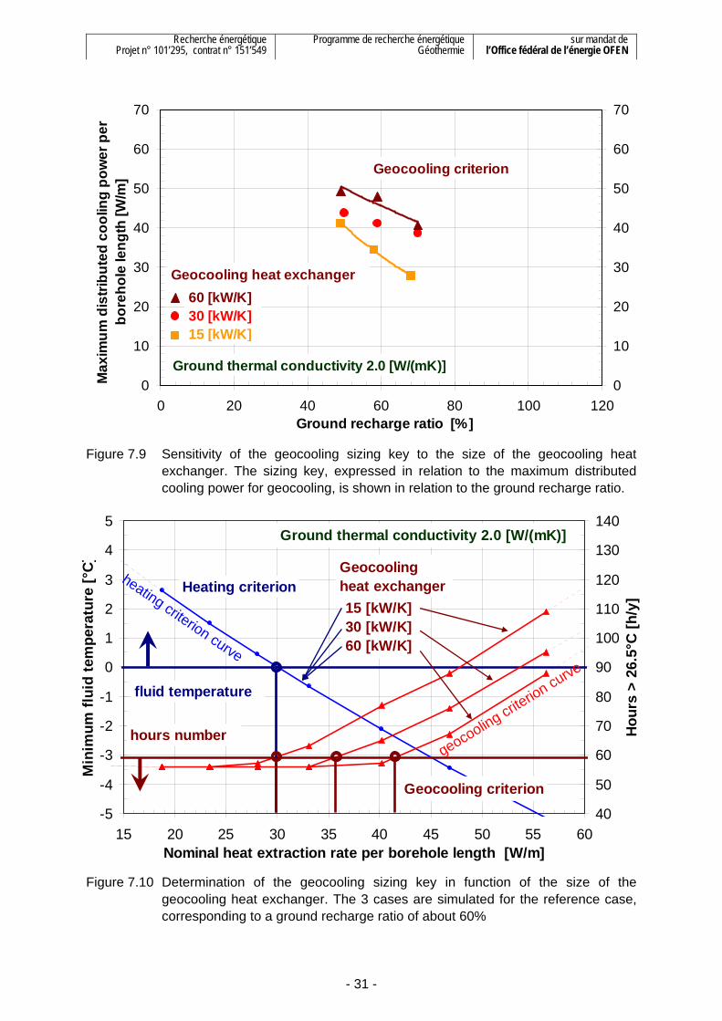
Recherche énergétique Projet n° 101’295, contrat n° 151’549
Programme de recherche énergétique Géothermie
sur mandat de l’Office fédéral de l’énergie OFEN
- 31 -
0
10
20
30
40
50
60
70
0 20 40 60 80 100 120Ground recharge ratio [%]
Max
imum
dis
tribu
ted
cool
ing
pow
er p
er
bore
hole
leng
th [W
/m]
0
10
20
30
40
50
60
70
Ground thermal conductivity 2.0 [W/(mK)]
Geocooling heat exchanger60 [kW/K]30 [kW/K]15 [kW/K]
Geocooling criterion
Figure 7.9 Sensitivity of the geocooling sizing key to the size of the geocooling heat
exchanger. The sizing key, expressed in relation to the maximum distributed cooling power for geocooling, is shown in relation to the ground recharge ratio.
Figure 7.10 Determination of the geocooling sizing key in function of the size of the geocooling heat exchanger. The 3 cases are simulated for the reference case, corresponding to a ground recharge ratio of about 60%
-5
-4
-3
-2
-1
0
1
2
3
4
5
15 20 25 30 35 40 45 50 55 60Nominal heat extraction rate per borehole length [W/m]
Min
imum
flui
d te
mpe
ratu
re [°
C]
40
50
60
70
80
90
100
110
120
130
140
Hou
rs >
26.
5°C
[h/y
]
Ground thermal conductivity 2.0 [W/(mK)]
fluid temperature
hours number
15 [kW/K]30 [kW/K]60 [kW/K]
Geocooling heat exchangerHeating criterion
Geocooling criterion
heating criterion curve
geocooling criterion curve

Recherche énergétique Projet n° 101’295, contrat n° 151’549
Programme de recherche énergétique Géothermie
sur mandat de l’Office fédéral de l’énergie OFEN
- 32 -
In figure 7.10 the graph permits to illustrate how the heating and geocooling sizing keys are determined for the variation of the heat transfer capacity of the geocooling heat exchanger.
The heating criterion curves are equal for the three values of the heat transfer capacity of the geocooling heat exchanger. As expected the geocooling heat exchanger size has no influence on the heating sizing key, assessed in this case to 30 W/m.
The geocooling criterion curves lead to the determination of three geocooling sizing keys, assessed to respectively 30, 36 and 46 W/m in function of the geocooling heat exchanger size, whose heat transfer capacity is set to respectively 15, 30 and 60 kW/K.
These sizing keys are calculated on the basis of the nominal heat extraction rate. They are then processed to be expressed in function of the maximum distributed cooling power. It has to be observed that the criterion curves are interpolated on the basis of a finite number of simulation results. As the heating criterion curve is quasi linear, the determination of the heating sizing key is rather precise. This is not the case with the geocooling criterion curves. Their bent shape is inducing some uncertainty in the determination of the geocooling sizing key.
In table 7.4 the results of the sensitivity analysis are shown in a qualitative way. The effect of a parameter change is indicated with a sign “+” for an augmentation or “–“ for a diminution. The effect on the sizing key is reported in the same way.
Effect due to parameter Parameter change Heating sizing key Geocooling sizing key
Ground recharge ratio + + + – – – Ground thermal conductivity + + + + + Initial ground temperature + + – –
Geocooling heat exchanger size – o – –
Borehole depth + + –
Borehole spacing + (+)* o * only for low ground recharge ratio Table 7.4 Results of the sensitivity analysis presented in a qualitative way.

Recherche énergétique Projet n° 101’295, contrat n° 151’549
Programme de recherche énergétique Géothermie
sur mandat de l’Office fédéral de l’énergie OFEN
- 33 -
8. Heating and geocooling capacity values
8.1 Geocooling temperature difference potential Geocooling is primarily conditioned by the available temperature difference between the desired indoor air temperature and the initial ground temperature. It defines the geocooling temperature difference potential. This temperature difference is divided between the building, including its cooling distribution and the geocooling heat exchanger, and the ground coupled system.
The reference building with the reference location is used to illustrate the various temperature losses (TAB-TRIPLE-GR50 in Chiasso, see chapter 5). They are shown in figure 8.1.
Temperature losses between indoor air and ground
10
15
20
25
30
Temperatures for geocooling
Tem
pera
ture
leve
l [°C
]
Building designCooling distributionGeocooling heat exchangerGround heat exchangerInitial ground temperature
Building
Ground
initial ground temperature
maximal fluid temperature level in BHE
water temperature level in cooling distribution
indoor set point temperature for cooling controlindoor air temperature
Figure 8.1 Temperature losses in the geocooling temperature difference potential. The fluid
temperature levels are defined as the average of their inlet and outlet values in the geocooling heat exchanger for the heat transfer of the maximum distributed cooling power.
The desired indoor air temperature is fixed to 26°C. The regulation of the cooling system is based on a set-point indoor air temperature to switch on cooling and a smaller one to switch it off. For the reference building they were fixed to respectively 25°C and 24°C. The average, 24.5°C, is the indoor set-point temperature level for cooling control. This first temperature loss (26°C – 24.5°C = 1.5 K) is necessary to keep some margin and anticipate the indoor air temperature increase due to internal and solar passive gains.
The second temperature loss is created by the cooling distribution. It is the difference between the indoor set point temperature and the water temperature level in the cooling distribution. This latter is defined as the average between the design forward water temperature in the cooling distribution (21°C) and the return one (23.5°C) at the maximum distributed cooling power (65 kW).

Recherche énergétique Projet n° 101’295, contrat n° 151’549
Programme de recherche énergétique Géothermie
sur mandat de l’Office fédéral de l’énergie OFEN
- 34 -
The third temperature loss is created by the geocooling heat exchanger. It is the difference between the water temperature level in the cooling distribution and the maximal fluid temperature level in the borehole heat exchangers (BHE). This latter is defined as the average between the maximum possible outlet fluid temperature from the BHE (18.8°C) and the maximum inlet fluid temperature in the BHE (21.3°C) at the maximum distributed cooling power (65 kW).
The sum of the first three temperature losses is called the building temperature difference.
The last temperature loss is caused by the ground heat exchanger. It is defined as the difference between the maximal fluid temperature level in the BHE and the initial ground temperature. This latter is obtained as the average temperature of the ground layer crossed by the boreholes (13.3°C), which corresponds to the first 100m for the reference case. This temperature loss is called the ground temperature difference.
Long term effects do not reduce the ground temperature difference as long as the ground recharge ratio is small enough and in any case not larger than 100%. For a too large ground recharge ratio the ground temperature in the ground volume enclosed by the BHE will tend to increase with years. As a consequence this long term temperature increase should be deducted from the ground temperature difference. Unless this correction is small, a geocooling solution is often not possible in this case.
A scarce building design requires greater cooling power to be extracted. As a result the temperature difference associated to the building has to be greater. A scarce cooling distribution design also requires a greater temperature difference to extract the same cooling power, increasing as well the temperature difference associated to the building. Finally a scarce geocooling heat exchanger creates a greater temperature loss that contributes to increase the building temperature difference. The available ground temperature difference, resulting from the difference between the geocooling and the building temperature difference, might be too small or even negative to make a geocooling solution technically feasible.
In the heating case, a heat pump separates the ground heat exchanger from the building and its heat distribution system, making the ground heat system less sensitive to the interaction with the building concept and design. This is the opposite in the geocooling case: the ground coupled system is highly dependent on the building design and its cooling distribution. The geocooling temperature difference potential is shared between the building and the ground. It is thus very important, when a geocooling system is designed, to have the possibility to modify and optimise to some extent both the building design and the cooling emitters, so that the best system integration can be obtained.
8.2 Definition of a geocooling capacity value The cooling power covered by geocooling results from a heat transfer governed by a temperature difference. As for a conventional heat exchanger, a heat transfer rate capacity can be defined, expressing the transferred heat rate per temperature unit of a representative temperature difference. Using the definition of the geocooling sizing key (cf. section 7.3) and the ground temperature difference (cf. section 8.1), the geocooling capacity value is defined as follow:
- Ki = qi / ΔTgrnd specific geocooling heat transfer rate capacity, called geocooling capacity value [W/m/K]

Recherche énergétique Projet n° 101’295, contrat n° 151’549
Programme de recherche énergétique Géothermie
sur mandat de l’Office fédéral de l’énergie OFEN
- 35 -
where qi = Pcool_max / Hg
qi maximum distributed cooling power per borehole length unit, called geocooling sizing key [W/m]
Pcool_max maximum effective distributed cooling power [W]
Hg total borehole length required for geocooling [m]
ΔTgrnd ground temperature difference, defined as the difference between the maximal fluid temperature level in the BHE and the initial ground temperature [K]
In table 8.1 the ground temperature difference is indicated for the 11 reference building cases with internal heat gains scaled from 60% to 140%. The building temperature difference and the maximum effective distributed cooling power are also indicated. The geocooling temperature difference potential is fixed to 12.8 K for all cases. It can be observed how the ground temperature difference is decreasing with increasing internal heat gains, as a consequence of the necessity to have a larger building temperature difference to extract the increased internal heat gains. On the other hand the maximum cooling power is increasing significantly. These two effects (smaller ground temperature difference and greater cooling power) are driving the total borehole length toward a significant large value.
TAB-TRIPLE-GR50
Location: Chiasso
Building temperature difference
Ground temperature difference ΔTgrnd
Maximum effective distributed cooling
power
Internal heat gains magnitude [K] [K] [kW]
60% 4.8 8.0 56
70% 4.7 8.1 46
80% 6.1 6.7 73
90% 6.0 6.8 66
95% 6.0 6.8 66
100% 6.0 6.8 65
105% 7.2 5.6 83
110% 7.2 5.6 83
120% 7.2 5.6 83
130% 8.4 4.4 98
140% 8.5 4.3 99 Table 8.1 Building and ground temperature difference for geocooling. The geocooling
temperature difference potential is equal to 12.8 K for all cases. The maximum effective distributed cooling powers, to which the geocooling capacity are referred to, are also indicated.

Recherche énergétique Projet n° 101’295, contrat n° 151’549
Programme de recherche énergétique Géothermie
sur mandat de l’Office fédéral de l’énergie OFEN
- 36 -
The geocooling capacity value should take into account conditions that affect the ground temperature difference, such as a different initial ground temperature or a deeper borehole. In figure 8.2 all the cases related to various initial ground temperatures and borehole depths are shown. The dispersion of the values prevents to detect any sensitivity of the geocooling capacity value to the ground temperature difference.
0
1
2
3
4
5
6
7
8
9
10
0 20 40 60 80 100 120Ground recharge ratio [%]
Geo
cool
ing
heat
tran
sfer
rate
cap
acity
pe
r bor
ehol
e le
ngth
[W/m
/K]
0
1
2
3
4
5
6
7
8
9
10
Ground thermal conductivity 2.0 [W/(mK)]
T ground surface 14 [°C], H 100mT ground surface 12 [°C], H 100mT ground surface 10 [°C], H 100mT ground surface 12 [°C], H 150m
Geocooling criterion
Figure 8.2 Geocooling capacity value shown in relation to the ground recharge ratio. The
sensitivity to the initial ground temperature and the borehole depth are not anymore noticeable.
In a similar way a geocooling capacity value can be defined for the annual geocooling energy. For all shown cases in figure 8.2 the values range from 2 to 4 [kWh/m/K/y].
To an internal heat gains magnitude of 120% corresponds a ground recharge ratio of 80%. Using a geocooling capacity value of 6 [W/m/K] for this ground recharge ratio, the borehole length can be recalculated with the help of the maximum effective distributed cooling power (Pcool_max) and the ground temperature difference (ΔTgrnd). Reading respectively 83 [kW] and 5.6 [K] from table 8.1, the total borehole length is estimated as follow:
- Hg = Pcool_max / Ki / ΔTgrnd = 83’000 [W] / 6 [W/m/K] / 5.6 [K] = 2’500 [m]

Recherche énergétique Projet n° 101’295, contrat n° 151’549
Programme de recherche énergétique Géothermie
sur mandat de l’Office fédéral de l’énergie OFEN
- 37 -
Assuming a value of 3 [kWh/m/K/y], the annual geocooling energy would be estimated to 3 [kWh/m/K/y] x 2500 [m] x 5.6 [K] = 42’000 [kWh/y].
In figure 8.3, the geocooling capacity value is shown for the various geocooling heat exchanger sizes. The results obtained with the larger geocooling heat exchanger remains within the design value range. Only the undersized geocooling heat exchangers exhibits larger values than the design ones. A small geocooling heat exchanger is decreasing the potential ground temperature difference. The design values, applied to a system having a small geocooling heat exchanger, would give a longer borehole length, to compensate for the smaller ground temperature difference. In this way they would provide a conservative borehole length.
0
1
2
3
4
5
6
7
8
9
10
0 20 40 60 80 100 120Ground recharge ratio [%]
Geo
cool
ing
heat
tran
sfer
rate
cap
acity
pe
r bor
ehol
e le
ngth
[W/m
/K]
0
1
2
3
4
5
6
7
8
9
10
Ground thermal conductivity 2.0 [W/(mK)]
60 kW/K30 kW/K15 kW/K
Geocooling criterion
Geocooling heat exchanger
Figure 8.3 Geocooling capacity value shown in relation to the ground recharge ratio.
Sensitivity to the size of the geocooling heat exchanger is only observable for the small heat exchanger size. A small geocooling heat exchanger is decreasing the ground temperature difference potential and thus increasing the total borehole length. The key values, applied to system having a small geocooling heat exchanger, would provide a conservative borehole length.
8.3 Geocooling sizing keys and capacity values for all simulated cases All simulated cases are listed in table 8.2. The table contains the design installed heating power, the maximum effective distributed cooling power, the design forward water temperature in the cooling distribution, the annual distributed cooling energy and the ground recharge ratio. In order not to have an unrealistic large maximum cooling power due to the heating and cooling conflict (see section 6.3), the maximum power value is assessed for the months of July and August only. This is particularly important for all cases with floor heating
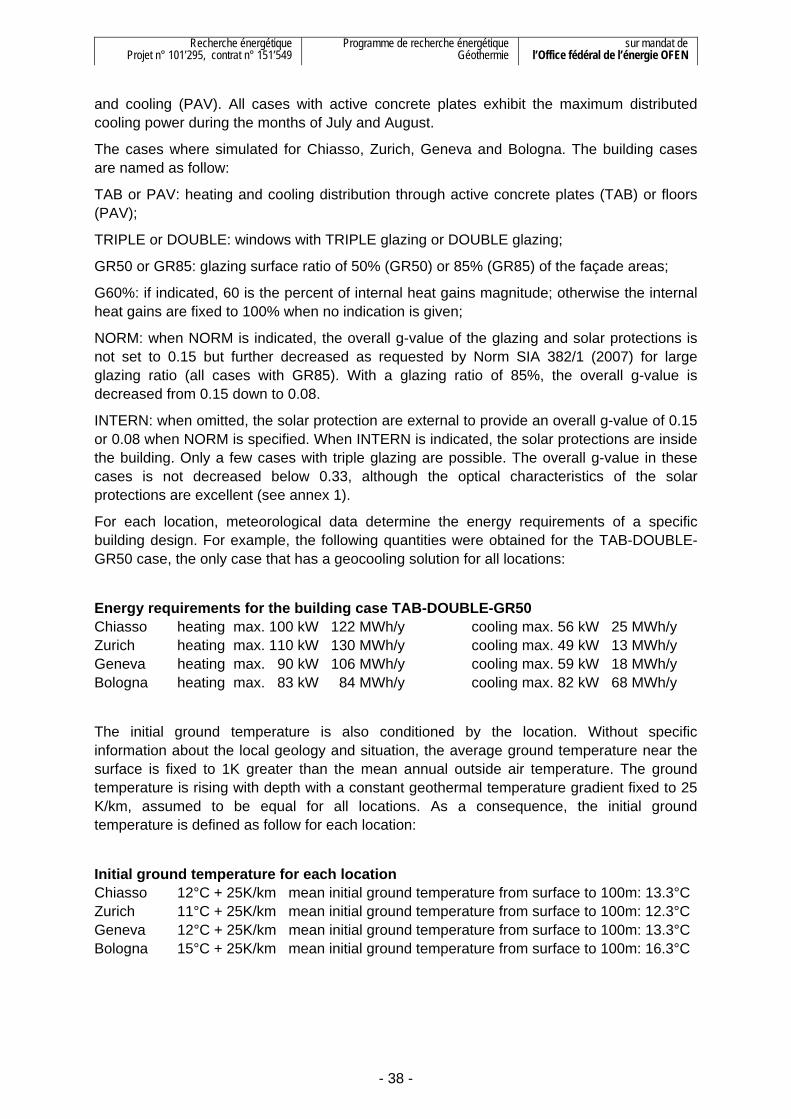
Recherche énergétique Projet n° 101’295, contrat n° 151’549
Programme de recherche énergétique Géothermie
sur mandat de l’Office fédéral de l’énergie OFEN
- 38 -
and cooling (PAV). All cases with active concrete plates exhibit the maximum distributed cooling power during the months of July and August.
The cases where simulated for Chiasso, Zurich, Geneva and Bologna. The building cases are named as follow:
TAB or PAV: heating and cooling distribution through active concrete plates (TAB) or floors (PAV);
TRIPLE or DOUBLE: windows with TRIPLE glazing or DOUBLE glazing;
GR50 or GR85: glazing surface ratio of 50% (GR50) or 85% (GR85) of the façade areas;
G60%: if indicated, 60 is the percent of internal heat gains magnitude; otherwise the internal heat gains are fixed to 100% when no indication is given;
NORM: when NORM is indicated, the overall g-value of the glazing and solar protections is not set to 0.15 but further decreased as requested by Norm SIA 382/1 (2007) for large glazing ratio (all cases with GR85). With a glazing ratio of 85%, the overall g-value is decreased from 0.15 down to 0.08.
INTERN: when omitted, the solar protection are external to provide an overall g-value of 0.15 or 0.08 when NORM is specified. When INTERN is indicated, the solar protections are inside the building. Only a few cases with triple glazing are possible. The overall g-value in these cases is not decreased below 0.33, although the optical characteristics of the solar protections are excellent (see annex 1).
For each location, meteorological data determine the energy requirements of a specific building design. For example, the following quantities were obtained for the TAB-DOUBLE-GR50 case, the only case that has a geocooling solution for all locations:
Energy requirements for the building case TAB-DOUBLE-GR50 Chiasso heating max. 100 kW 122 MWh/y cooling max. 56 kW 25 MWh/y Zurich heating max. 110 kW 130 MWh/y cooling max. 49 kW 13 MWh/y Geneva heating max. 90 kW 106 MWh/y cooling max. 59 kW 18 MWh/y Bologna heating max. 83 kW 84 MWh/y cooling max. 82 kW 68 MWh/y
The initial ground temperature is also conditioned by the location. Without specific information about the local geology and situation, the average ground temperature near the surface is fixed to 1K greater than the mean annual outside air temperature. The ground temperature is rising with depth with a constant geothermal temperature gradient fixed to 25 K/km, assumed to be equal for all locations. As a consequence, the initial ground temperature is defined as follow for each location:
Initial ground temperature for each location Chiasso 12°C + 25K/km mean initial ground temperature from surface to 100m: 13.3°C Zurich 11°C + 25K/km mean initial ground temperature from surface to 100m: 12.3°C Geneva 12°C + 25K/km mean initial ground temperature from surface to 100m: 13.3°C Bologna 15°C + 25K/km mean initial ground temperature from surface to 100m: 16.3°C

Recherche énergétique Projet n° 101’295, contrat n° 151’549
Programme de recherche énergétique Géothermie
sur mandat de l’Office fédéral de l’énergie OFEN
- 39 -
Building thermal requirements Design installed heating power
Maximum effective
distributed cooling power
Design forward cooling
tempera-ture
Annual distributed
cooling energy
Ground recharge
ratio
Location and building case [kW] [kW] [°C] [MWh/y] [%]
CHIASSO
TAB-TRIPLE-GR50 G60% 77 56 22 20 25 TAB-TRIPLE-GR50 G70% 75 46 22 25 33 TAB-TRIPLE-GR50 G80% 75 73 21 28 37 TAB-TRIPLE-GR50 G90% 75 66 21 34 50 TAB-TRIPLE-GR50 G95% 75 66 21 36 54 TAB-TRIPLE-GR50 G100% 75 65 21 38 59 TAB-TRIPLE-GR50 G105% 75 83 20 43 66 TAB-TRIPLE-GR50 G110% 75 83 20 45 70 TAB-TRIPLE-GR50 G120% 75 83 20 49 81 TAB-TRIPLE-GR50 G130% 75 98 19 58 91 TAB-TRIPLE-GR50 G140% 75 99 19 66 102
PAV-TRIPLE-GR50 G60% 75 48 22 19 23 PAV-TRIPLE-GR50 G80% 75 66 21 29 36 PAV-TRIPLE-GR50 G90% 75 84 20 37 47 PAV-TRIPLE-GR50 G100% 75 76 20 62 67 PAV-TRIPLE-GR50 G110% 75 75 19 66 72
PAV-DOUBLE-GR50 100 75 20 45 37 PAV-TRIPLE-GR50 75 76 20 41 65 TAB-DOUBLE-GR50 100 56 22 25 26 TAB-TRIPLE-GR50 75 65 21 36 62 TAB-TRIPLE-GR85 NORM 70 46 22 30 60 TAB-TRIPLE-GR85 75 48 20 57 118 TAB-TRIPLE-GR50 INTERN 75 88 18 87 197 Table 8.2 Main thermal requirements of the simulated cases that have a geocooling
solution (part 1). The design heat extraction rate is obtained with the design installed heating power and a COP of 4.
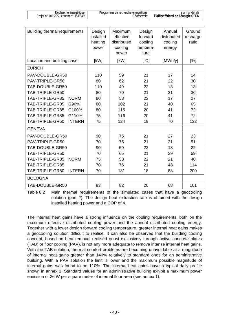
Recherche énergétique Projet n° 101’295, contrat n° 151’549
Programme de recherche énergétique Géothermie
sur mandat de l’Office fédéral de l’énergie OFEN
- 40 -
Building thermal requirements Design installed heating power
Maximum effective
distributed cooling power
Design forward cooling
tempera-ture
Annual distributed
cooling energy
Ground recharge
ratio
Location and building case [kW] [kW] [°C] [MWh/y] [%]
ZURICH
PAV-DOUBLE-GR50 110 59 21 17 14 PAV-TRIPLE-GR50 80 62 21 22 30 TAB-DOUBLE-GR50 110 49 22 13 13 TAB-TRIPLE-GR50 80 70 21 21 36 TAB-TRIPLE-GR85 NORM 80 53 22 17 27 TAB-TRIPLE-GR85 G90% 80 102 21 40 65 TAB-TRIPLE-GR85 G100% 80 115 20 41 72 TAB-TRIPLE-GR85 G110% 75 116 20 41 72 TAB-TRIPLE-GR50 INTERN 75 124 19 70 132
GENEVA
PAV-DOUBLE-GR50 90 75 21 27 23 PAV-TRIPLE-GR50 70 75 21 31 51 TAB-DOUBLE-GR50 90 59 22 18 22 TAB-TRIPLE-GR50 70 65 21 29 59 TAB-TRIPLE-GR85 NORM 75 53 22 21 40 TAB-TRIPLE-GR85 70 76 21 48 114 TAB-TRIPLE-GR50 INTERN 70 131 18 88 200
BOLOGNA
TAB-DOUBLE-GR50 83 82 20 68 101 Table 8.2 Main thermal requirements of the simulated cases that have a geocooling
solution (part 2). The design heat extraction rate is obtained with the design installed heating power and a COP of 4.
The internal heat gains have a strong influence on the cooling requirements, both on the maximum effective distributed cooling power and the annual distributed cooling energy. Together with a lower design forward cooling temperature, greater internal heat gains makes a geocooling solution difficult to realise. It can also be observed that the building cooling concept, based on heat removal realised quasi exclusively through active concrete plates (TAB) or floor cooling (PAV), is not any more adequate to remove intense internal heat gains. With the TAB solution, thermal comfort problems are becoming unavoidable at a magnitude of internal heat gains greater than 140% relatively to standard ones for an administrative building. With a PAV solution the limit is lower and the maximum possible magnitude of internal gains was found to be 110%. The internal heat gains have a typical daily profile shown in annex 1. Standard values for an administrative building exhibit a maximum power emission of 26 W per square meter of internal floor area (see annex 1).
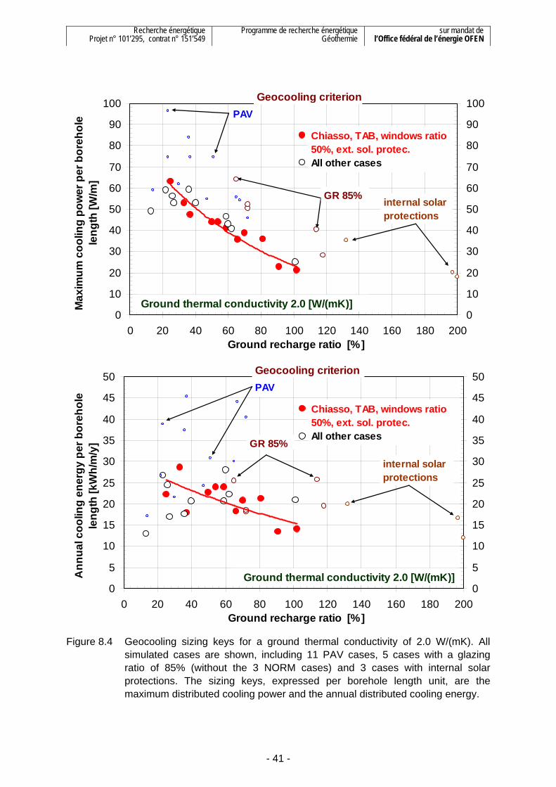
Recherche énergétique Projet n° 101’295, contrat n° 151’549
Programme de recherche énergétique Géothermie
sur mandat de l’Office fédéral de l’énergie OFEN
- 41 -
0
10
20
30
40
50
60
70
80
90
100
0 20 40 60 80 100 120 140 160 180 200Ground recharge ratio [%]
Max
imum
coo
ling
pow
er p
er b
oreh
ole
leng
th [W
/m]
0
10
20
30
40
50
60
70
80
90
100
Ground thermal conductivity 2.0 [W/(mK)]
Geocooling criterion
Chiasso, TAB, windows ratio 50%, ext. sol. protec.All other cases
internal solar protections
PAV
GR 85%
0
5
10
15
20
25
30
35
40
45
50
0 20 40 60 80 100 120 140 160 180 200Ground recharge ratio [%]
Ann
ual c
oolin
g en
ergy
per
bor
ehol
e le
ngth
[kW
h/m
/y]
0
5
10
15
20
25
30
35
40
45
50
Ground thermal conductivity 2.0 [W/(mK)]
Geocooling criterion
Chiasso, TAB, windows ratio 50%, ext. sol. protec.All other cases
internal solar protections
PAV
GR 85%
Figure 8.4 Geocooling sizing keys for a ground thermal conductivity of 2.0 W/(mK). All
simulated cases are shown, including 11 PAV cases, 5 cases with a glazing ratio of 85% (without the 3 NORM cases) and 3 cases with internal solar protections. The sizing keys, expressed per borehole length unit, are the maximum distributed cooling power and the annual distributed cooling energy.
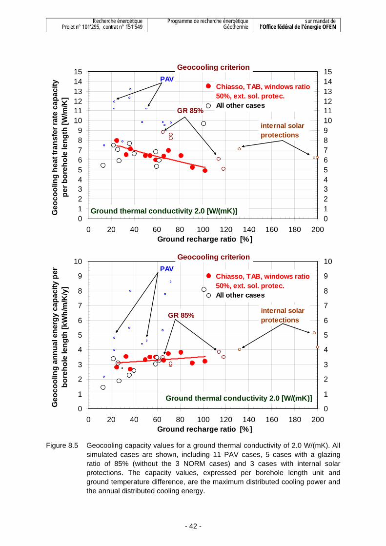
Recherche énergétique Projet n° 101’295, contrat n° 151’549
Programme de recherche énergétique Géothermie
sur mandat de l’Office fédéral de l’énergie OFEN
- 42 -
0123456789
101112131415
0 20 40 60 80 100 120 140 160 180 200Ground recharge ratio [%]
Geo
cool
ing
heat
tran
sfer
rate
cap
acity
pe
r bor
ehol
e le
ngth
[W/m
/K]
0123456789101112131415
Ground thermal conductivity 2.0 [W/(mK)]
Geocooling criterion
Chiasso, TAB, windows ratio 50%, ext. sol. protec.All other cases
internal solar protections
PAV
GR 85%
0
1
2
3
4
5
6
7
8
9
10
0 20 40 60 80 100 120 140 160 180 200Ground recharge ratio [%]
Geo
cool
ing
annu
al e
nerg
y ca
paci
ty p
er
bore
hole
leng
th [k
Wh/
m/K
/y]
0
1
2
3
4
5
6
7
8
9
10
Ground thermal conductivity 2.0 [W/(mK)]
Geocooling criterion
Chiasso, TAB, windows ratio 50%, ext. sol. protec.All other cases
internal solar protections
PAV
GR 85%
Figure 8.5 Geocooling capacity values for a ground thermal conductivity of 2.0 W/(mK). All
simulated cases are shown, including 11 PAV cases, 5 cases with a glazing ratio of 85% (without the 3 NORM cases) and 3 cases with internal solar protections. The capacity values, expressed per borehole length unit and ground temperature difference, are the maximum distributed cooling power and the annual distributed cooling energy.

Recherche énergétique Projet n° 101’295, contrat n° 151’549
Programme de recherche énergétique Géothermie
sur mandat de l’Office fédéral de l’énergie OFEN
- 43 -
The sizing values obtained with the active concrete plate solutions (TAB) are more conservative than the one obtained with heating and cooling floor (PAV). However TAB solutions can provide a geocooling solution to a wider range of building designs, including larger glazing ratio, such as the GR85 cases.
At low ground recharge ratio, the lower sizing values are not accurate, as the optimal borehole length would have been smaller than the smallest simulated borehole length. As a result the values are smaller that what they should be. They are in any case not relevant as the borehole sizing, with such a small ground recharge ratio, is based on the heating criterion and not the geocooling one.
The geocooling capacity values, which take into account the ground temperature difference, present a weaker dependence to the ground recharge ratio than the geocooling sizing keys.
For a ground thermal conductivity of 2 W/(mK), a conservative specific geocooling capacity value of 5 W/m/K can be used for all simulated cases.
8.4 Heat extraction temperature difference potential The same approach can be applied for heating. In this case a heat pump separates the heating building distribution system from the borehole flow circuit. The magnitude of the heat extraction rate is primarily conditioned by the available temperature difference between initial ground temperature and minimum allowed fluid temperature level in the borehole flow circuit, called ground heat exchanger. It defines the heat extraction temperature difference potential. This temperature difference is divided between the long term temperature drift and the short term temperature difference for heat extraction.
The reference building with the reference location is used to illustrate the magnitude of these two temperature losses (TAB-TRIPLE-GR50 in Chiasso, see chapter 5). They were obtained for a ground ratio of about 60%. The temperature losses are shown in figure 8.6.
Temperature losses between ground and BHE fluid
0
5
10
15
20
Temperatures for heat extraction
Tem
pera
ture
leve
l [°C
]
Long term temperature driftGround heat exchangerMinimum fluid temperature
Ground
initial ground temperature
minimal fluid temperature level in BHE
long term mean temperature drift in the ground
Figure 8.6 Temperature losses in the heat extraction temperature difference potential. The
fluid temperature level is defined as the average of the inlet and outlet value in the ground heat exchanger.
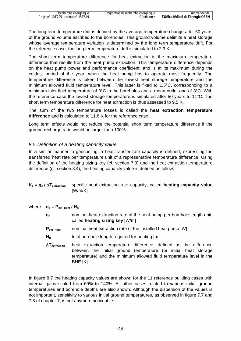
Recherche énergétique Projet n° 101’295, contrat n° 151’549
Programme de recherche énergétique Géothermie
sur mandat de l’Office fédéral de l’énergie OFEN
- 44 -
The long term temperature drift is defined by the average temperature change after 50 years of the ground volume ascribed to the boreholes. This ground volume delimits a heat storage whose average temperature variation is determined by the long term temperature drift. For the reference case, the long term temperature drift is simulated to 2.3 K.
The short term temperature difference for heat extraction is the maximum temperature difference that results from the heat pump extraction. This temperature difference depends on the heat pump power and performance coefficient, and is at its maximum during the coldest period of the year, when the heat pump has to operate most frequently. The temperature difference is taken between the lowest heat storage temperature and the minimum allowed fluid temperature level. This latter is fixed to 1.5°C, corresponding to a minimum inlet fluid temperature of 0°C in the boreholes and a mean outlet one of 3°C. With the reference case the lowest storage temperature is simulated after 50 years to 11°C. The short term temperature difference for heat extraction is thus assessed to 9.5 K.
The sum of the two temperature losses is called the heat extraction temperature difference and is calculated to 11.8 K for the reference case.
Long term effects would not reduce the potential short term temperature difference if the ground recharge ratio would be larger than 100%.
8.5 Definition of a heating capacity value In a similar manner to geocooling, a heat transfer rate capacity is defined, expressing the transferred heat rate per temperature unit of a representative temperature difference. Using the definition of the heating sizing key (cf. section 7.3) and the heat extraction temperature difference (cf. section 8.4), the heating capacity value is defined as follow:
Ke = qe / ΔTextraction specific heat extraction rate capacity, called heating capacity value [W/m/K]
where qe = Pext_nom / Hh
qe nominal heat extraction rate of the heat pump per borehole length unit, called heating sizing key [W/m]
Pext_nom nominal heat extraction rate of the installed heat pump [W]
Hh total borehole length required for heating [m]
ΔTextraction heat extraction temperature difference, defined as the difference between the initial ground temperature (or initial heat storage temperature) and the minimum allowed fluid temperature level in the BHE [K]
In figure 8.7 the heating capacity values are shown for the 11 reference building cases with internal gains scaled from 60% to 140%. All other cases related to various initial ground temperatures and borehole depths are also shown. Although the dispersion of the values is not important, sensitivity to various initial ground temperatures, as observed in figure 7.7 and 7.8 of chapter 7, is not anymore noticeable.

Recherche énergétique Projet n° 101’295, contrat n° 151’549
Programme de recherche énergétique Géothermie
sur mandat de l’Office fédéral de l’énergie OFEN
- 45 -
A smaller ground recharge ratio means a smaller annual recharge of the ground. The short term temperature difference for heat extraction is decreasing as the long term temperature drift is increasing. The heating capacity value has to decrease with a smaller ground recharge ratio (i.e. an increasing long term temperature drift), as the heat extraction temperature difference does not take into account long term effect. The overall trend appears to be rather linear.
0
1
2
3
4
5
0 20 40 60 80 100 120Ground recharge ratio [%]
Des
ign
heat
ext
ract
ion
rate
cap
acity
per
bo
reho
le le
ngth
[W/m
/K]
0
1
2
3
4
5
Ground thermal conductivity 2.0 [W/(mK)]
T ground surface 14 [°C], H 100mT ground surface 12 [°C], H 100mT ground surface 10 [°C], H 100mT ground surface 12 [°C], H 150m
Heating criterion for Tmin inlet fluid 0°C
Figure 8.7 Heating capacity value shown in relation to the ground recharge ratio. The
sensitivity to the initial ground temperature and the borehole depth are not anymore noticeable.
In a similar way a heating capacity value can be defined for the annual extracted energy. For all shown cases in figure 8.7 the values range from 2.2 to 3.4 [kWh/m/K/y].
8.6 Heating and geocooling keys for all simulated cases The required bore lengths for all simulated cases are given in table 8.3. The table contains the heating sizing keys, the total borehole lengths to satisfy the heating criterion, the geocooling sizing keys, the total borehole lengths to satisfy the geocooling criterion and the ground recharge ratio. The cases are the same as those listed in table 8.2. The meaning of the nomenclature can be found in section 8.3 and the design heating and cooling requirements in table 8.2.
The results are simulated for the following ground and borehole conditions:
- average ground thermal conductivity 2 W/(mK)
- minimum return fluid temperature in boreholes 0°C

Recherche énergétique Projet n° 101’295, contrat n° 151’549
Programme de recherche énergétique Géothermie
sur mandat de l’Office fédéral de l’énergie OFEN
- 46 -
- borehole depth 100 m
- average borehole spacing 8 m
Sizing keys and total borehole length
Ground 2 W/(mK), bore depth 100 m and spacing 8m
Heating sizing key
Bore length for heating criterion
Geocooling sizing key
Bore length for
geocooling criterion
Ground recharge
ratio
Location and building case [W/m] [m] [W/m] [m] [%]
CHIASSO
TAB-TRIPLE-GR50 G60% 23 2’500 63 900 25 TAB-TRIPLE-GR50 G70% 24 2’300 53 900 33 TAB-TRIPLE-GR50 G80% 25 2’200 47 1’500 37 TAB-TRIPLE-GR50 G90% 29 1’900 44 1’500 50 TAB-TRIPLE-GR50 G95% 29 1’900 44 1’500 54 TAB-TRIPLE-GR50 G100% 30 1’900 41 1’600 59 TAB-TRIPLE-GR50 G105% 32 1’800 36 2’300 66 TAB-TRIPLE-GR50 G110% 33 1’700 39 2’100 70 TAB-TRIPLE-GR50 G120% 35 1’600 36 2’300 81 TAB-TRIPLE-GR50 G130% 36 1’600 23 4’300 91 TAB-TRIPLE-GR50 G140% 38 1’500 21 4’700 102
PAV-TRIPLE-GR50 G60% 24 2’400 96 500 23 PAV-TRIPLE-GR50 G80% 27 2’100 84 800 36 PAV-TRIPLE-GR50 G90% 30 1’900 55 1’500 47 PAV-TRIPLE-GR50 G100% 34 1’700 54 1’400 67 PAV-TRIPLE-GR50 G110% 35 1’600 46 1’600 72
PAV-DOUBLE-GR50 24 3’100 75 1’000 37 PAV-TRIPLE-GR50 36 1’600 56 1’400 65 TAB-DOUBLE-GR50 22 3’400 56 1’000 26 TAB-TRIPLE-GR50 31 1’800 41 1’600 62 TAB-TRIPLE-GR85 NORM 31 1’700 43 1’100 60 TAB-TRIPLE-GR85 38 1’500 28 2’900 118 TAB-TRIPLE-GR50 INTERN 39 1’500 20 5’200 197 Table 8.3 Heating and geocooling sizing keys together with borehole length for all
simulated cases. The bore lengths were rounded to plus or minus 100 m (part 1).

Recherche énergétique Projet n° 101’295, contrat n° 151’549
Programme de recherche énergétique Géothermie
sur mandat de l’Office fédéral de l’énergie OFEN
- 47 -
Sizing keys and total borehole length
Ground 2 W/(mK), bore depth100 m and spacing 8m
Heating sizing key
Bore length for heating criterion
Geocooling sizing key
Bore length for
geocooling criterion
Ground recharge
ratio
Location and building case [W/m] [m] [W/m] [m] [%]
ZURICH
PAV-DOUBLE-GR50 18 4’700 59 1’000 14 PAV-TRIPLE-GR50 24 2’500 62 1’000 30 TAB-DOUBLE-GR50 17 4’800 49 1’000 13 TAB-TRIPLE-GR50 24 2’600 59 1’200 36 TAB-TRIPLE-GR85 NORM 23 2’600 53 1’000 27 TAB-TRIPLE-GR85 G90% 29 2’100 64 1’600 65 TAB-TRIPLE-GR85 G100% 30 2’000 50 2’300 72 TAB-TRIPLE-GR85 G110% 29 1’900 52 2’200 72 TAB-TRIPLE-GR50 INTERN 34 1’700 35 3’500 132
GENEVA
PAV-DOUBLE-GR50 21 3’200 75 1’000 23 PAV-TRIPLE-GR50 32 1’600 75 1’000 51 TAB-DOUBLE-GR50 22 3’100 59 1’000 22 TAB-TRIPLE-GR50 30 1’700 46 1’400 59 TAB-TRIPLE-GR85 NORM 29 1’900 53 1’000 40 TAB-TRIPLE-GR85 38 1’400 41 1’900 114 TAB-TRIPLE-GR50 INTERN 38 1’400 18 7’300 200
BOLOGNA
TAB-DOUBLE-GR50 44 1’400 25 3’300 101 Table 8.3 Heating and geocooling sizing keys together with borehole length for all
simulated cases. The bore lengths were rounded to plus or minus 100 m (part 2).
For the Swiss location like Zurich, Geneva and Chiasso, the use of triple instead of double glazing has the advantage to halve the total required borehole length. Two effects are beneficial: the maximum heating power is smaller and allows for a reduction of the borehole length as sizing is conditioned by the heating criterion. The second important effect is the ground recharge ratio which is at least doubled, leading to a substantial reduction of the long term effects, thus reducing the total borehole length as sizing is still conditioned by the heating criterion.
For the Italian location of Bologna, this is the opposite. The only possible solution is obtained with double glazing, otherwise the ground recharge ratio would be far too large. In this case and as expected, sizing is conditioned by the geocooling criterion. It can be observed how the total required borehole length is large, indicating that geocooling solutions with BHE has reached its southern limit with a climat such as the one in Bologna.
Recherche énergétique Projet n° 101’295, contrat n° 151’549
Programme de recherche énergétique Géothermie
sur mandat de l’Office fédéral de l’énergie OFEN
- 48 -
In figure 8.8 to 8.13, geocooling and heating sizing keys are shown for all simulated cases and various conditions. The heating criterion is presented for both a minimum return fluid temperature in the borehole of 0°C and -3°C.
Figure 8.8: ground thermal conductivity of 1.5 W/(mK) – geocooling and heating sizing keys
Figure 8.9: ground thermal conductivity of 1.5 W/(mK) – geocool. and heat. capacity values
Figure 8.10: ground thermal conductivity of 2.0 W/(mK) – geocooling and heating sizing keys
Figure 8.11: ground thermal conductivity of 2.0 W/(mK) – geocool. and heat. capacity values
Figure 8.12: ground thermal conductivity of 3.0 W/(mK) – geocooling and heating sizing keys
Figure 8.13: ground thermal conductivity of 3.0 W/(mK) – geocool. and heat. capacity values
The heating capacity values, which take into account the temperature difference between the initial ground temperature and the minimum tolerated fluid temperature in the borehole flow circuit, do not exhibit similar values when the minimum return fluid temperature in the boreholes is fixed to 0°C or -3°C.
A detailed analysis revealed that half of the difference is explained with the heat extraction rate of the heat pump. The heating capacity value are calculated with the nominal heat extraction rate, based on the nominal heat pump COP and power, and not on the effective values. If the heat pump is working with an inlet fluid temperature of -3°C instead of 0°C in the evaporator, the heat extraction rate is smaller, allowing for a shorter borehole length (Hh), thus increasing the heating capacity value (Ke), even if the heat extraction temperature difference (ΔTextraction) is the same for both cases.
The other half of the difference is related to the boundary conditions at the ground surface, including the horizontal connexions between the boreholes.
Secondly the definition of a temperature difference for the calculation of a heat transfer capacity value is difficult when it has to be based only on design data. A more appropriate definition would probably require a simulation of the system first, which is obviously not the scope for a fast estimation of a pre-design sizing.
The heating and geocooling capacity values, determined for a particular project, are not universal. They certainly help for pre-design purposes, but do not substitute simulations for system sizing.
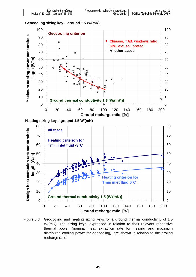
Recherche énergétique Projet n° 101’295, contrat n° 151’549
Programme de recherche énergétique Géothermie
sur mandat de l’Office fédéral de l’énergie OFEN
- 49 -
0
10
20
30
40
50
60
70
80
90
100
0 20 40 60 80 100 120 140 160 180 200Ground recharge ratio [%]
Max
imum
coo
ling
pow
er p
er b
oreh
ole
leng
th [W
/m]
0
10
20
30
40
50
60
70
80
90
100
Ground thermal conductivity 1.5 [W/(mK)]
Geocooling criterion
Chiasso, TAB, windows ratio 50%, ext. sol. protec.All other cases
0
10
20
30
40
50
60
70
80
0 20 40 60 80 100 120 140 160 180 200Ground recharge ratio [%]
Des
ign
heat
ext
ract
ion
rate
per
bor
ehol
e le
ngth
[W/m
]
0
10
20
30
40
50
60
70
80
Ground thermal conductivity 1.5 [W/(mK)]
Heating criterion for Tmin inlet fluid -3°C
All cases
Heating criterion for Tmin inlet fluid 0°C
Figure 8.8 Geocooling and heating sizing keys for a ground thermal conductivity of 1.5
W/(mK). The sizing keys, expressed in relation to their relevant respective thermal power (nominal heat extraction rate for heating and maximum distributed cooling power for geocooling), are shown in relation to the ground recharge ratio.
Geocooling sizing key – ground 1.5 W/(mK)
Heating sizing key – ground 1.5 W/(mK)

Recherche énergétique Projet n° 101’295, contrat n° 151’549
Programme de recherche énergétique Géothermie
sur mandat de l’Office fédéral de l’énergie OFEN
- 50 -
0123456789
101112131415
0 20 40 60 80 100 120 140 160 180 200Ground recharge ratio [%]
Geo
cool
ing
heat
tran
sfer
rate
cap
acity
pe
r bor
ehol
e le
ngth
[W/m
/K]
0123456789101112131415
Ground thermal conductivity 1.5 [W/(mK)]
Geocooling criterion Chiasso, TAB, windows ratio 50%, ext. sol. protec.All cases
0
1
2
3
4
5
0 20 40 60 80 100 120 140 160 180 200Ground recharge ratio [%]
Des
ign
heat
ext
ract
ion
rate
cap
acity
per
bo
reho
le le
ngth
[W/m
/K]
0
1
2
3
4
5
Ground thermal conductivity 1.5 [W/(mK)]
Heating criterion for Tmin inlet fluid -3°C
Heating criterion for Tmin inlet fluid 0°C
All cases
Figure 8.9 Geocooling and heating capacity values for a ground thermal conductivity of 1.5
W/(mK). The sizing keys, expressed in relation to their relevant respective thermal power (nominal heat extraction rate for heating and maximum distributed cooling power for geocooling), are shown in relation to the ground recharge ratio.
Geocooling capacity value – ground 1.5 W/(mK)
Heating capacity value – ground 1.5 W/(mK)

Recherche énergétique Projet n° 101’295, contrat n° 151’549
Programme de recherche énergétique Géothermie
sur mandat de l’Office fédéral de l’énergie OFEN
- 51 -
0
10
20
30
40
50
60
70
80
90
100
0 20 40 60 80 100 120 140 160 180 200Ground recharge ratio [%]
Max
imum
coo
ling
pow
er p
er b
oreh
ole
leng
th [W
/m]
0
10
20
30
40
50
60
70
80
90
100
Ground thermal conductivity 2.0 [W/(mK)]
Geocooling criterion
Chiasso, TAB, windows ratio 50%, ext. sol. protec.All other cases
0
10
20
30
40
50
60
70
80
0 20 40 60 80 100 120 140 160 180 200Ground recharge ratio [%]
Des
ign
heat
ext
ract
ion
rate
per
bor
ehol
e le
ngth
[W/m
]
0
10
20
30
40
50
60
70
80
Ground thermal conductivity 2.0 [W/(mK)]
Heating criterion for Tmin inlet fluid -3°C
All cases
Heating criterion for Tmin inlet fluid 0°C
Figure 8.10 Geocooling and heating sizing keys for a ground thermal conductivity of 2.0
W/(mK). The sizing keys, expressed in relation to their relevant respective thermal power (nominal heat extraction rate for heating and maximum distributed cooling power for geocooling), are shown in relation to the ground recharge ratio.
Geocooling sizing key – ground 2.0 W/(mK)
Heating sizing key – ground 2.0 W/(mK)
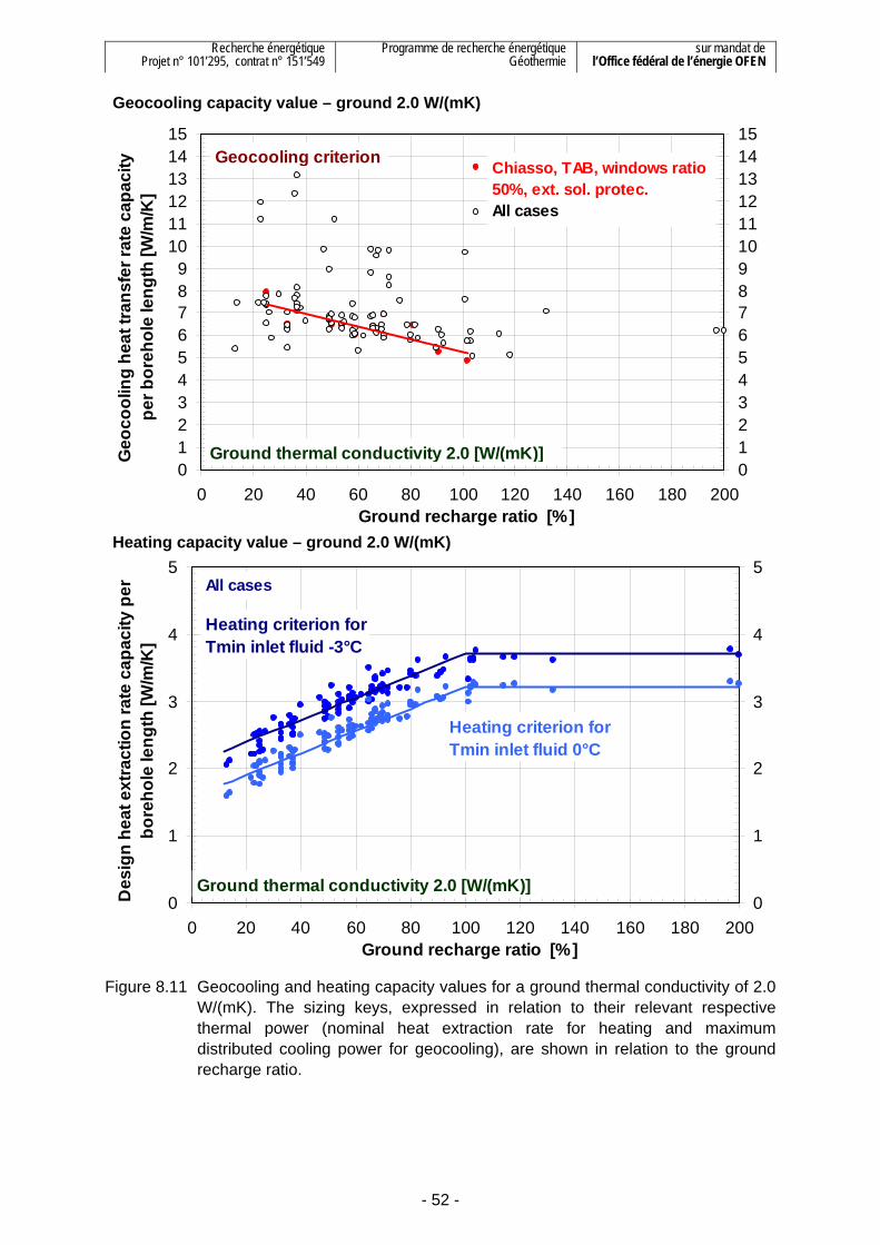
Recherche énergétique Projet n° 101’295, contrat n° 151’549
Programme de recherche énergétique Géothermie
sur mandat de l’Office fédéral de l’énergie OFEN
- 52 -
0123456789
101112131415
0 20 40 60 80 100 120 140 160 180 200Ground recharge ratio [%]
Geo
cool
ing
heat
tran
sfer
rate
cap
acity
pe
r bor
ehol
e le
ngth
[W/m
/K]
0123456789101112131415
Ground thermal conductivity 2.0 [W/(mK)]
Geocooling criterion Chiasso, TAB, windows ratio 50%, ext. sol. protec.All cases
0
1
2
3
4
5
0 20 40 60 80 100 120 140 160 180 200Ground recharge ratio [%]
Des
ign
heat
ext
ract
ion
rate
cap
acity
per
bo
reho
le le
ngth
[W/m
/K]
0
1
2
3
4
5
Ground thermal conductivity 2.0 [W/(mK)]
Heating criterion for Tmin inlet fluid -3°C
Heating criterion for Tmin inlet fluid 0°C
All cases
Figure 8.11 Geocooling and heating capacity values for a ground thermal conductivity of 2.0
W/(mK). The sizing keys, expressed in relation to their relevant respective thermal power (nominal heat extraction rate for heating and maximum distributed cooling power for geocooling), are shown in relation to the ground recharge ratio.
Geocooling capacity value – ground 2.0 W/(mK)
Heating capacity value – ground 2.0 W/(mK)

Recherche énergétique Projet n° 101’295, contrat n° 151’549
Programme de recherche énergétique Géothermie
sur mandat de l’Office fédéral de l’énergie OFEN
- 53 -
0
10
20
30
40
50
60
70
80
90
100
0 20 40 60 80 100 120 140 160 180 200Ground recharge ratio [%]
Max
imum
coo
ling
pow
er p
er b
oreh
ole
leng
th [W
/m]
0
10
20
30
40
50
60
70
80
90
100
Ground thermal conductivity 3.0 [W/(mK)]
Geocooling criterion
Chiasso, TAB, windows ratio 50%, ext. sol. protec.All other cases
0
10
20
30
40
50
60
70
80
0 20 40 60 80 100 120 140 160 180 200Ground recharge ratio [%]
Des
ign
heat
ext
ract
ion
rate
per
bor
ehol
e le
ngth
[W/m
]
0
10
20
30
40
50
60
70
80
Ground thermal conductivity 3 [W/(mK)]
Heating criterion for Tmin inlet fluid -3°CAll cases
Heating criterion for Tmin inlet fluid 0°C
Figure 8.12 Geocooling and heating sizing keys for a ground thermal conductivity of 3.0
W/(mK). The sizing keys, expressed in relation to their relevant respective thermal power (nominal heat extraction rate for heating and maximum distributed cooling power for geocooling), are shown in relation to the ground recharge ratio.
Geocooling sizing key – ground 3.0 W/(mK)
Heating sizing key – ground 3.0 W/(mK)

Recherche énergétique Projet n° 101’295, contrat n° 151’549
Programme de recherche énergétique Géothermie
sur mandat de l’Office fédéral de l’énergie OFEN
- 54 -
0123456789
101112131415
0 20 40 60 80 100 120 140 160 180 200Ground recharge ratio [%]
Geo
cool
ing
heat
tran
sfer
rate
cap
acity
pe
r bor
ehol
e le
ngth
[W/m
/K]
0123456789101112131415
Ground thermal conductivity 3.0 [W/(mK)]
Geocooling criterion Chiasso, TAB, windows ratio 50%, ext. sol. protec.All cases
0
1
2
3
4
5
0 20 40 60 80 100 120 140 160 180 200Ground recharge ratio [%]
Des
ign
heat
ext
ract
ion
rate
cap
acity
per
bo
reho
le le
ngth
[W/m
/K]
0
1
2
3
4
5
Ground thermal conductivity 3 [W/(mK)]
Heating criterion for Tmin inlet fluid -3°C
Heating criterion for Tmin inlet fluid 0°C
All cases
Figure 8.13 Geocooling and heating capacity values for a ground thermal conductivity of 3.0
W/(mK). The sizing keys, expressed in relation to their relevant respective thermal power (nominal heat extraction rate for heating and maximum distributed cooling power for geocooling), are shown in relation to the ground recharge ratio.
Geocooling capacity value – ground 3.0 W/(mK)
Heating capacity value – ground 3.0 W/(mK)

Recherche énergétique Projet n° 101’295, contrat n° 151’549
Programme de recherche énergétique Géothermie
sur mandat de l’Office fédéral de l’énergie OFEN
- 55 -
8.7 Pre-sizing example In this section, a pre-sizing example of a geocooling application is described to illustrate the use of design data values given in the previous section. The use of the design data values has to be done with extremely careful prudence. The similitude between the project described in this study and a new project has to be good enough. A pre-sizing made with the design data values can not, in any case, substitute thermal simulations done for sizing purposes.
The information about the project to be sized is given as follow: Building thermal requirements: Installed heat pump power at nominal condition (B0W35): 90 kW Number of operating hours per year at nominal power : 1’200 h/y Nominal heat pump performance coefficient (COP) : 4.5 - Maximum distributed cooling power: 80 kW Number of operating hours per year at nominal power : 500 h/y Design forward fluid temperature in cooling distribution : 20 °C Ground thermal characteristics: Average ground thermal conductivity: 2 W/(mK) Initial ground temperature near ground surface : 12 °C Mean geothermal temperature gradient : 25 K/km Borehole heat exchangers: Borehole heat exchanger type: double-U pipe Borehole depth : 100 m Average borehole spacing : 8 m Position of the boreholes : under the building Some assumptions are made to be able to use the basic project information: The nominal heat pump power corresponds to the maximum heat power demand of the building. Mean annual seasonal factor or performance coefficient : 4.5 - (without circulation pump electric energy) Return design fluid temperature from cooling distribution : 23 °C Geocooling heat exchanger design temperature loss : 2 K Minimum inlet fluid temperature in the boreholes : 0 °C Corresponding outlet fluid temperature from the boreholes : 3 °C Determinant design quantities:
From these quantities the determinant design quantities can be calculated: Nominal heat extraction rate of the installed heat pump Pext_nom 70 kW Annual energy extracted from the ground: 84 MWh/y Maximum effective distributed cooling power Pcool_max 80 kW Annual geocooling energy injected in the ground: 40 MWh/y Ground recharge ratio: 48%
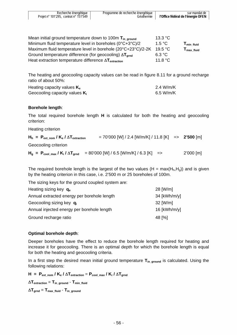
Recherche énergétique Projet n° 101’295, contrat n° 151’549
Programme de recherche énergétique Géothermie
sur mandat de l’Office fédéral de l’énergie OFEN
- 56 -
Mean initial ground temperature down to 100m Tin_ground 13.3 °C Minimum fluid temperature level in boreholes (0°C+3°C)/2 1.5 °C Tmin_fluid Maximum fluid temperature level in borehole (20°C+23°C)/2-2K 19.5 °C Tmax_fluid Ground temperature difference (for geocooling) ΔTgrnd 6.3 °C Heat extraction temperature difference ΔTextraction 11.8 °C
The heating and geocooling capacity values can be read in figure 8.11 for a ground recharge ratio of about 50%: Heating capacity values Ke 2.4 W/m/K Geocooling capacity values Ki 6.5 W/m/K
Borehole length:
The total required borehole length H is calculated for both the heating and geocooling criterion:
Heating criterion
Hh = Pext_nom / Ke / ΔTextraction = 70’000 [W] / 2.4 [W/m/K] / 11.8 [K] => 2’500 [m]
Geocooling criterion
Hg = Pcool_max / Ki / ΔTgrnd = 80’000 [W] / 6.5 [W/m/K] / 6.3 [K] => 2’000 [m]
The required borehole length is the largest of the two values (H = max(Hh,Hg)) and is given by the heating criterion in this case, i.e. 2’500 m or 25 boreholes of 100m.
The sizing keys for the ground coupled system are: Heating sizing key qe 28 [W/m] Annual extracted energy per borehole length 34 [kWh/m/y] Geocooling sizing key qi 32 [W/m] Annual injected energy per borehole length 16 [kWh/m/y]
Ground recharge ratio 48 [%]
Optimal borehole depth:
Deeper boreholes have the effect to reduce the borehole length required for heating and increase it for geocooling. There is an optimal depth for which the borehole length is equal for both the heating and geocooling criteria.
In a first step the desired mean initial ground temperature Tin_ground is calculated. Using the following relations:
H = Pext_nom / Ke / ΔTextraction = Pcool_max / Ki / ΔTgrnd
ΔTextraction = Tin_ground - Tmin_fluid
ΔTgrnd = Tmax_fluid - Tin_ground

Recherche énergétique Projet n° 101’295, contrat n° 151’549
Programme de recherche énergétique Géothermie
sur mandat de l’Office fédéral de l’énergie OFEN
- 57 -
The desired mean initial ground temperature is calculated with:
Tin_ground = (Tmax_fluid x Ki/Pcool_max + Tmin_fluid x Ke/Pext_nom) / (Ki/Pcool_max + Ke/Pext_nom)
Tin_ground = 14.2 °C
To this mean initial ground temperature corresponds a depth of 170m and a minimum total required borehole length of 2’300 m.
Ground recharge ratio:
The ground recharge ratio has an influence on the heating and geocooling capacity values which is particularly strong on the heating one. The required borehole length is assessed for a variation of +/- 0.2 on the ground recharge ratio. It would typically correspond to a much smaller or larger operation time of the cooling mode (+/- 200 hours per year for the assumed value of 500 hours per years). It is important to notice that the maximum effective distributed power and the design forward fluid temperature in the cooling distribution are not changed.
The heating and geocooling capacity values are read in figure 8.11 in function of the ground recharge ratio. The values are shown in table 8.4.
Ground recharge ratio 30% 50% 70%
Heating capacity value Ke [W/m/K] 2.0 2.4 2.8 Geocooling capacity value Ki [W/m/K] 7.0 6.5 6.0 Table 8.4 Heating and geocooling capacity values in function of the ground recharge ratio.
The sizing results are shown in table 8.5. Ground recharge ratio 30% 50% 70%
Borehole length for heating criterion [m] 2’800 2’500 2’200 Borehole length for geocooling criterion [m] 1’800 2’000 2’100
Required borehole length with 100 meter deep boreholes [m] 3’000 2’500 2’100 Optimal borehole depth [m] 240 170 120 Required borehole length with optimal borehole depth [m] 2’500 2’300 2’200 Table 8.5 Required borehole length in function of the ground recharge ratio.
The ground recharge ratio has a substantial influence on the required borehole length, especially at low ratio value, due to the large influence of the long term effects if the ground recharge ratio is low. The annual cooling energy covered by geocooling is thus an important quantity to assess, as it has a direct influence on the ground recharge ratio.

Recherche énergétique Projet n° 101’295, contrat n° 151’549
Programme de recherche énergétique Géothermie
sur mandat de l’Office fédéral de l’énergie OFEN
- 58 -
Design forward fluid temperature in the cooling distribution:
The required borehole length for geocooling is strongly dependent on the maximum cooling power and the design forward fluid temperature in the cooling distribution. This latter conditions the maximum possible fluid temperature level in the borehole flow circuit. The required borehole length is assessed for a variation of +/- 2 K on the design forward fluid temperature in the cooling distribution. It is important to notice that the maximum effective distributed power is not changed. A different forward fluid temperature to distribute the same cooling power means a design difference in the cooling distribution, such as the area for example.
The specific heat extraction and geocooling heat rate capacities are read in figure 8.11 in function of the ground recharge ratio. The values are shown in table 8.6.
Design forward temperature 18 °C 20 °C 22 °C
Ground temperature difference ΔTgrnd [K] 4.3 6.3 8.3 Table 8.6 Ground temperature difference in function of the design forward fluid
temperature in the cooling distribution.
The sizing results are shown in table 8.7. Design forward temperature 18 °C 20 °C 22 °C
Borehole length for heating criterion [m] 2’500 2’500 2’500 Borehole length for geocooling criterion [m] 2’900 2’000 1’500
Required borehole length with 100 meter deep boreholes [m] 2’900 2’500 2’500 Optimal borehole depth [m] 60 170 280 Required borehole length with optimal borehole depth [m] 2’600 2’300 2’100 Table 8.7 Required borehole length in function of the design forward fluid temperature in
the cooling distribution.
The design forward fluid temperature in the cooling distribution has a strong influence on the required borehole length to satisfy the geocooling criterion. In addition to a significant longer total bore length, a lower design forward temperature is decreasing the possibility to drill deep boreholes. It is thus very important not to design cooling distribution systems with low fluid temperature or with a non necessary low forward fluid temperature value.

Recherche énergétique Projet n° 101’295, contrat n° 151’549
Programme de recherche énergétique Géothermie
sur mandat de l’Office fédéral de l’énergie OFEN
- 59 -
9. Conclusions
A complete system simulation tool for an office building, its heating and cooling distribution and a geocooling system with borehole heat exchangers has been developed, taking the benefice of existing and well established tools. A detailed methodology has been developed for building analysis and assessment of its suitability to be cooled by geocooling. Sizing of the ground coupled system for heating and geocooling is then carried out in a consecutive step.
Definitions of sizing keys and capacity values for heating and geocooling were proposed to show the results of all simulations. They were executed for different building locations, building designs, distribution types, borehole configurations and local ground conditions.
The results were presented to provide simple and fast design guidelines for a pre-sizing of a geocooling system.
At the building level, geocooling is feasible if the building concept comply to a low energy standard, the solar protections fulfil the SIA 382/1 Norm requirements, and the internal heat gains do not considerably exceed typical values for an administrative building. A large internal mass or thermal capacity is an advantage, although an average value is sufficient. A medium internal thermal capacity is normally obtained if active concrete plates are used. Active concrete plates are the most suitable distribution system to minimize both heating and cooling annual distributed energies. Their auto-regulating properties are a key factor to avoid heating and cooling conflict during midseason.
Best geocooling systems are obtained at a ground recharge ratio of about 50%. The use of triple instead of double glazing allows for peak power reduction and makes the ground ratio increase. As a result the total borehole length is halved for all systems having a low ground recharge ratio with double glazing windows. Another key parameter that conditions the geocooling potential is the temperature difference between design forward fluid temperature in cooling distribution and the initial ground temperature. The higher the design forward cooling temperature the greater the cooling potential. Active concrete plates, allowing for high distribution temperatures, are most suitable for a geocooling application.
The available simple design rules enables a fast pre-sizing of a geocooling system. However they do not substitute a proper system simulation. It is important to have the possibility to simulate, as no generalisation can be stated. A simulation should be done in any case to validate the pre-design sizing. As a by-product of this research project, the COOLSIM2 tool is available for ulterior studies of such geocooling applications.
10. Acknowledgement
The Swiss Federal Office of Energy is acknowledged for its financial support without which this study would not have been possible. Every person who took part in the study is also warmly acknowledged.

Recherche énergétique Projet n° 101’295, contrat n° 151’549
Programme de recherche énergétique Géothermie
sur mandat de l’Office fédéral de l’énergie OFEN
- 60 -
11. References • Chuard P., Chuard D., Van Gilst J., Hadorn J.-C. and Mercier C. (1983) The IEA Task
VII Swiss project in Vaulruz: design and first experiences. International conference on subsurface heat storage in theory and practice. pp. 195 – 206. Swedish Coucil for Building Research.
• GSP(2011) Groupement promotionnel Suisse pour les pompes à chaleur. www.pac.ch
• Hellström G. (1989) Duct Ground Heat Storage Model, Manual for Computer Code. Department of Mathematical Physics, University of Lund, Sweden.
• Hollmuller P., Lachal B. et Pahud D. (2005) Rafraîchissement par geocooling. Bases pour un manuel de dimensionnement. Rapport final, Office Fédéral de l’Energie, Berne, Suisse.
• ISO 13786 (2007) Thermal performance of building components – Dynamic thermal characteristics – Calculation methods. International Organisation for Standardization, Geneva, Switzerland.
• Klein S. A. et al. (2007) TRNSYS. A Transient System Simulation Program. Version 16.1. Solar Energy Laboratory, University of Wisconsin, Madison, USA.
• Pahud D. (1993) Etude du Centre Industriel et Artisanal Marcinhès à Meyrin (GE). Rapport final. GAP et CUEPE, Univ. de Genève.
• Pahud D. and Hellström G. (1996) The New Duct Ground Heat Model for TRNSYS. EUROTHERM, Physical Models for Thermal Energy Stores. A.A. van Steenhoven and W.G.L van Helden (eds), March 25-27, pp. 127 – 136, Eindhoven, The Netherlands.
• Pahud D., Fromentin A. and Hadorn J.-C. (1996) The Duct Ground Heat Storage Model (DST) for TRNSYS Used for the Simulation of Heat Exchanger Piles. User Manual, December 1996 Version. Internal Report. LASEN - DGC- EPFL, Switzerland.
• Pahud D. et Travaglini G. (2000) Etude d’une maison solaire active avec stockage en dalles au Tessin. Rapport final, Office fédéral de l’énergie, Berne, Suisse.
• Pahud D. (2007) PILESIM2: Simulation Tool for Heating/Cooling Systems with Energy Piles or multiple Borehole Heat Exchangers. User Manual. ISAAC – DACD – SUPSI, Switzerland.
• Pahud D. (2007) BRIDGESIM : Simulation Tool for the System Design of Bridge Heating for Ice Prevention with Solar Heat Stored in a Seasonal Ground Duct Store. User Manual. ISAAC – DACD – SUPSI, Switzerland.
• Pahud D. (2008) COOLSIM : Simulation Tool for the System Design of Borehole Heat Exchangers or Energy Piles for Geocooling with TABS in Office Building. User Manual. ISAAC – DACD – SUPSI, Switzerland.
• Pahud D., Caputo P., Branca G. et Generelli M. (2008) Etude du potentiel d’utilisation de “geocooling” d’une installation avec sondes géothermiques verticales appliqué à un bâtiment administratif Minergie à Chiasso. Rapport final, Office fédéral de l’énergie, Berne, Suisse.
• SIA Cahier Technique 2024 (2006) Conditions d’utilisation standard pour l’énergie et les installations du bâtiment, Société suisse des ingénieurs et des architectes, Zurich, Suisse.

Recherche énergétique Projet n° 101’295, contrat n° 151’549
Programme de recherche énergétique Géothermie
sur mandat de l’Office fédéral de l’énergie OFEN
- 61 -
• SIA Norm 382/1 (2007) Lüftungs- und Klimaanlagen – Allgemeine Grundlagen und Anforderungen, Schweizerischer Ingenieur- und Architektenverein Zürich, Schweiz.
• SIA Norme 384/6 (2010) Sondes géothermiques, Société suisse des ingénieurs et des architectes, Zurich, Suisse.

Manuale per il raffreddamento di edifici tramite « geocooling » con sonde geotermiche verticali
Allegato 1
L’edificio amministrativo di riferimento
Indice
A1.1. Edificio amministrativo di riferimento 1
A1.1.1. Involucro e dimensioni 1 A1.1.2. Qualità dell’involucro 2 A1.1.3. Protezioni solari 3 A1.1.4. Analisi delle protezioni solari secondo la norma UNI EN 13363-1 8 A1.1.5. Guadagni interni 14 A1.1.6. Ventilazione 15 A1.1.7. Capacità termica interna 16
A1.2. Riferimenti 16
Rapporto finale D. Pahud e M. Belliardi


Recherche énergétique Projet n° 101’295, contrat n° 151’549
Programme de recherche énergétique Géothermie
sur mandat de l’Office fédéral de l’énergie OFEN
A1.1. Edificio amministrativo di riferimento
L’edificio amministrativo Minergie® della dogana commerciale di Chiasso-Brogeda è preso quale riferimento per la definizione geometrica e strutturale degli edifici amministrativi simulati nel quadro di questo studio. Un vantaggio di questa scelta è che questo edificio è già stato ampiamente documentato e studiato in un precedente progetto mirato a valutare la fattibilità tecnica del geocooling (Pahud e al., 2008).
Buone premesse per il geocooling sono un involucro che soddisfa lo standard a basso consumo energetico Minergie® ed un erogazione dell’energia termica con delle solette termo-attive. In altre parole conferisce un’inerzia termica molto grande tra la produzione di energia e la sua erogazione, e permette di mandare l’acqua nelle solette a delle temperature molto vicine a quelle degli ambienti riscaldati e raffreddati.
A1.1.1. Involucro e dimensioni L’edificio è caratterizzato da una forma piuttosto compatta ed allungata. Ha una sezione di 440 m2 (53m x 8.4 m) ed un’altezza di 16.6 m, avendo così 5 piani di forma rettangolare.
Le superfici dell’involucro ed il volume riscaldato sono elencati nella Tabella A1.1 :
Superficie di riferimento energetico (SRE) 2'200 m2
Volume netto riscaldato 5'700 m3
Facciata Est superficie totale
superficie apertura finestre
140 m2
70 m2
Facciata Sud superficie totale facciata
superficie apertura finestre
880 m2
440 m2
Facciata Ovest superficie totale facciata
superficie apertura finestre
140 m2
70 m2
Facciata Nord superficie totale facciata
superficie apertura finestre
880 m2
440 m2
Tetto superficie verso esterno 440 m2
Pavimento superficie verso non riscaldato
superficie verso terreno
120 m2
320 m2
Tabella A1.1 : Dati relativi a volumi e superfici.
- A1.1 -

Recherche énergétique Projet n° 101’295, contrat n° 151’549
Programme de recherche énergétique Géothermie
sur mandat de l’Office fédéral de l’énergie OFEN
A1.1.2. Qualità dell’involucro Le pareti ed il tetto dell’edificio, in calcestruzzo armato, sono isolati all’esterno (vedi Pahud e al. (2008) per la stratigrafia dei muri). Nel caso base di riferimento, i vetri corrispondono a quelli di un triplo vetro, il cui valore g corrisponde a 0.4. Il valore g è, per definizione, il grado di trasmissione energetica dell’irraggiamento solare incidente sul piano vetrato. Sono anche prese in considerazione delle varianti di edifici con un doppio vetro avente valore g di 0.6. Le caratteristiche degli elementi dell’involucro sono elencati nella Tabella A1.2.
Elemento costruttivo Valore U [W/(m2K)]
Pareti esterne 1.0
Tetto 0.2
Pavimento verso locale non riscaldato
0.3
Pavimento verso terreno 0.3
Vetro triplo (caso base di riferimento)
0.7
Vetro doppio (variante del caso base)
1.4
Tabella A1.2 : Valore U delle pareti esterne, dei pavimenti, del tetto e dei vetri.
Le pareti esterne opache sono isolate con uno strato di isolamento di ca. 12-14 cm. Il valore U complessivo è elevato perché le superfici opache includono il telaio delle finestre.
- A1.2 -

Recherche énergétique Projet n° 101’295, contrat n° 151’549
Programme de recherche énergétique Géothermie
sur mandat de l’Office fédéral de l’énergie OFEN
A1.1.3. Protezioni solari La norma SIA 382/1 (2007) impone dei vincoli sul valore massimo per il g-value globale della finestra. I locali in cui è necessario o comunque si desidera il raffreddamento devono infatti essere conformi alle condizioni di protezione solare imposte dalla norma.
Secondo l’orientamento e la percentuale di superficie vetrata fg della facciata, le finestre con gli appositi dispositivi di protezione solare devono avere un coefficiente g globale che soddisfa le seguenti condizioni:
- facciate N g ≤ MIN (0,20/fg; 1,00)
- facciate NE e NO g ≤ MIN (0,13/fg; 0,28)
- facciate E, SE, S, SO, O g ≤ MIN (0,07/fg; 0,15)
Figura A1.1 : Valore limite del g-value in funzione della percentuale di facciata vetrata e
dell’orientamento (grafico da norma SIA 382/1:2007).
Le tipologie di edifici simulati possiedono delle percentuali di superfici vetrate del 50% e dell’85% in facciata, questo implica dei valori g globali da osservare rispettivamente di circa 0.15 e 0.08. L’edificio di riferimento ha una percentuale di superfici vetrate del 50%.
Sono state effettuate delle simulazioni dinamiche per valutare la variazione del valore g del vetro di una finestra adottando differenti protezioni solari. Sono quindi state utilizzate sia delle protezioni solari interne, cioè sul lato interno della finestra, che delle protezioni solari esterne.
- A1.3 -

Recherche énergétique Projet n° 101’295, contrat n° 151’549
Programme de recherche énergétique Géothermie
sur mandat de l’Office fédéral de l’énergie OFEN
Una protezione solare, come ad esempio una tenda, può coprire parzialmente oppure totalmente una finestra, si è quindi calcolato il valore g risultante con diversi gradi di apertura di una protezione solare, per due diversi tipi di vetro con caratteristiche termiche differenti.
I due vetri utilizzati nelle simulazioni sono il DOUBLE ed il TRIPLE, che presentano le seguenti caratteristiche (secondo programma Windows 5 (2008)) :
vetro ID U-value [W/m2K]
g-value [%/100]
DOUBLE 2004 1.4 0.622
TRIPLE 4001 0.68 0.407 Tabella A1.3 : Tipi di vetro utilizzati con le rispettive proprietà termiche.
Protezione solare interna
Sono state utilizzate, per una prima serie di simulazioni, tre diverse tende quali protezioni solari interne, che hanno i seguenti coefficienti adimensionali di trasmissione, riflessione ed assorbimento:
Tenda
SOLTIS 86 Tenda
simulata 1 Tenda
translucida trasmissione τ 0.22 0.10 0.25 riflessione ρ 0.42 0.45 0.60 assorbimento α 0.36 0.45 0.15
Tabella A1.4 : Tre diverse protezioni solari con le rispettive proprietà ottiche.
I parametri da immettere in TRNBuild del software TRNSYS (Klein e al., 2007), utilizzati per la simulazione dinamica dell’edificio, sono delle combinazioni di questi coefficienti e si inseriscono quando si caratterizza il tipo di vetro. Questi due parametri sono chiamati dal programma “Internal Shading Factor” e “Reflection Coefficient of Internal Device”, e vengono rispettivamente definiti come:
( ) 101)( ≤≤−⋅= zconzzISHADE τ
( )τρ−
=1
REFLISHADE
Essendo z l’abbassamento della protezione solare interna (cioè z=0 tenda completamente alzata, z=1 tenda completamente abbassata), è possibile notare che solamente il parametro ISHADE dipende dal grado di abbassamento di una protezione solare; ne deriva che il REFLISHADE è sempre costante per una stessa tenda, indipendentemente dal fatto che sia abbassata oppure no.
È possibile vedere, nei grafici delle figure A1.2 e A1.3, la dipendenza del valore g in funzione del grado di abbassamento della tenda (cioè area coperta dalla tenda su area dell’intero vetro). I due grafici rappresentano ognuno un tipo diverso di vetro (DOUBLE e TRIPLE), con i quali sono state simulate le tre protezioni solari aventi differenti proprietà trasmissive e riflessive.
- A1.4 -

Recherche énergétique Projet n° 101’295, contrat n° 151’549
Programme de recherche énergétique Géothermie
sur mandat de l’Office fédéral de l’énergie OFEN
g-value del DOUBLE per diversi gradi di protezione interna
0.250.300.350.400.450.500.550.600.650.700.750.80
0 0.2 0.4 0.6 0.8
chiusura [area tenda / area vetro]
g-va
lue
1
tenda SOLTIS 86tenda simulata 1
tenda traslucida
Figura A1.2 : Valore g del vetro DOUBLE per diversi gradi di protezione solare interna
delle tre differenti tende.
g-value del TRIPLE per diversi gradi di protezione interna
0.250.300.350.400.450.500.550.600.650.700.750.80
0 0.2 0.4 0.6 0.8 1chiusura [area tenda / area vetro]
g-va
lue
tenda SOLTIS 86tenda simulata 1tenda traslucida
Figura A1.3 : Valore g del vetro TRIPLE per diversi gradi di protezione solare interna delle
tre differenti tende.
Si può facilmente notare come la tenda traslucida, che possiede un elevato coefficiente di riflessione ed un basso coefficiente di assorbimento, sia la migliore nel tentare di abbassare il valore g in funzione del proprio grado di chiusura.
- A1.5 -

Recherche énergétique Projet n° 101’295, contrat n° 151’549
Programme de recherche énergétique Géothermie
sur mandat de l’Office fédéral de l’énergie OFEN
È quindi evidente che la variazione del valore g globale è poco dipendente dalla presenza di una tenda interna, la quale permette quindi una minima possibilità di regolazione dei guadagni solari.
Siccome in TRNBuild è necessario inserire il valore di ISHADE per definire la frazione di protezione solare, è stato fatto un grafico che raggruppa i due vetri utilizzati con la protezione interna “tenda simulata 1”. Questa tenda è stata scelta per le protezioni solari interne dell’edificio, ed è così possibile ottenere la correlazione tra il parametro da inserire nella simulazione (cioè l’ISHADE), ed il valore voluto in uscita del g-value.
g-value - ISHADE
0.00
0.10
0.20
0.30
0.40
0.50
0.60
0.70
0.80
0.90
0.00 0.10 0.20 0.30 0.40 0.50 0.60 0.70 0.80 0.90ISHADE
g-va
lue
DOUBLE
TRIPLE
Figura A1.4 : Valore g del vetro in funzione dell’ISHADE per i vetri DOUBLE e TRIPLE con
la protezione interna chiamata “tenda simulata 1”.
Siccome il coefficiente di trasmissione τ per questa tenda vale 0.1, l’intervallo possibile di valori di ISHADE varia da 0 a 0.9. Questi valori sono esattamente gli “Internal Shading Factor” da inserire nel TRNBuild.
Per le simulazioni con TRNSYS si sono cercati dei valori di ISHADE che permettano al g-value di non superare il valore di 0.15 (secondo la norma SIA 382/1:2007). Tuttavia, solamente con le protezioni solari interne, non risulta possibile abbassare il g-value globale a 0.15. Per questo motivo nel modello è stato inserito, sia per il vetro doppio che per il vetro triplo, un valore per l’ISHADE pari a 0.9, che permette di ottenere la miglior protezione possibile.
- A1.6 -

Recherche énergétique Projet n° 101’295, contrat n° 151’549
Programme de recherche énergétique Géothermie
sur mandat de l’Office fédéral de l’énergie OFEN
Protezione solare esterna
Nel TRNBuild è inoltre possibile inserire, per le superfici vetrate, delle protezioni solari esterne, le cui prestazioni sono definite impostando un valore desiderato di ESHADE (nel programma questo parametro da fissare è chiamato ”External Shading Factor”).
Questo parametro può variare da 0 a 1, senza avere informazioni sul tipo di protezione solare, sono state così effettuate delle simulazioni in modo da poter rappresentare la dipendenza del valore g da ESHADE per i due vetri DOUBLE e TRIPLE.
g-value - ESHADE
0.00
0.100.20
0.30
0.400.50
0.60
0.700.80
0.90
0.0 0.1 0.2 0.3 0.4 0.5 0.6 0.7 0.8 0.9 1.0ESHADE
g-va
lue
DOUBLE
TRIPLE
Figura A1.5 : Valore g del vetro in funzione di ESHADE per i vetri DOUBLE e TRIPLE.
È possibile notare una correlazione puramente lineare tra ESHADE ed il g-value globale; in particolare il valore g corrisponde a quello del vetro senza nessuna protezione esterna quando ESHADE è uguale a 0, mentre si arriva ad avere un g-value globale nullo nel caso in cui ESHADE è impostato sul suo valore massimo di 1.
Per semplicità questi fattori potrebbero anche essere visti come delle percentuali di riduzione del valore g, tant’è che ad esempio un ESHADE di 0.5 riduce della metà il g-value (-50%), mentre un ESHADE di 1 lo annulla completamente (-100%).
Anche nel caso di protezioni solari esterne, per poter soddisfare i requisiti imposti dalla norma SIA 382/1:2007, nella simulazione dinamica con TRNSYS si sono cercati dei parametri che caratterizzino le protezioni solari, e che permettano al g-value globale di non superare il valore limite di 0.15; come è possibile notare dal grafico in Figura A1.5, otteniamo un ESHADE uguale a 0.64 per il vetro triplo ed uno uguale 0.77 per il vetro doppio.
- A1.7 -

Recherche énergétique Projet n° 101’295, contrat n° 151’549
Programme de recherche énergétique Géothermie
sur mandat de l’Office fédéral de l’énergie OFEN
A1.1.4. Analisi delle protezioni solari secondo la norma UNI EN 13363-1 La norma tecnica europea UNI EN 13363-1 (2004) permette di stimare la trasmissione di energia solare totale di un dispositivo di protezione solare combinato con una superficie vetrata, utilizzando un metodo semplificato basato sulla trasmittanza termica e la trasmissione di energia solare totale del vetro, e sulla riflessione e trasmissione luminosa di un dispositivo di protezione solare.
Il metodo descritto nella norma, e poi utilizzato in questo lavoro, può essere applicato a protezioni solari, sia interne che esterne, il cui posizionamento risulti parallelo a quello del vetro.
Nella norma si è assunto che per i dispositivi esterni di protezione solare tra la schermatura ed il vetro lo spazio è non-ventilato, al contrario per i dispositivi interni lo spazio è ventilato.
I g-values risultanti dal metodo semplificato sono approssimati, e la loro deviazione dal valore esatto rientra in un range di errore compreso tra + 0.10 e - 0.02. I risultati tendono generalmente a rimanere sul lato della sicurezza per la stima dei carichi termici per il raffreddamento.
Protezioni solari esterne
Nel modello TRNSYS utilizzato è possibile inserire solamente un valore di ESHADE opportunamente scelto, in modo che permetta di ottenere un determinato g-value globale, ad esempio non superiore a 0.15, come nel caso simulato precedentemente (vedi Figura A1.5). Tuttavia questa procedura non permette di avere la sensibilità, o comunque la conoscenza, sui valori dei coefficienti ottici legati al tipo di protezione solare esterna.
È stata fatta per questo motivo un’analisi in modo da ottenere un “range” possibile di coefficienti ottici di trasmissione e riflessione, che soddisfino il vincolo dettato dalla norma SIA, in modo da valutare quali e che tipi di protezioni solari esterne possano essere idonee al caso.
Sono qui di seguito riportati due grafici, rispettivamente per i vetri DOUBLE e TRIPLE precedentemente descritti (Tabella A1.1), sui quali è possibile individuare l’intervallo possibile dei coefficienti di prestazione delle protezioni solari esterne, che permettono di ottenere un g-value globale inferiore a 0.15:
- A1.8 -
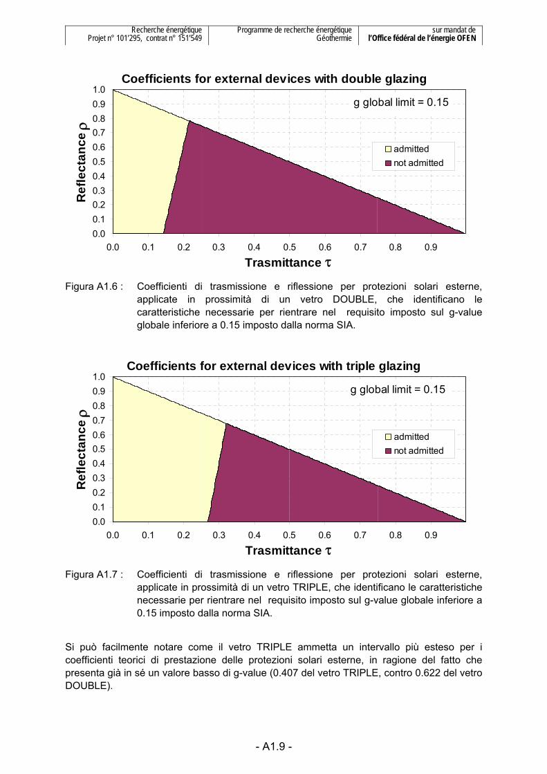
Recherche énergétique Projet n° 101’295, contrat n° 151’549
Programme de recherche énergétique Géothermie
sur mandat de l’Office fédéral de l’énergie OFEN
Coefficients for external devices with double glazing
0.00.10.20.30.40.50.60.70.80.91.0
0.0 0.1 0.2 0.3 0.4 0.5 0.6 0.7 0.8 0.9
Trasmittance τ
Ref
lect
ance
ρ
admittednot admitted
g global limit = 0.15
Figura A1.6 : Coefficienti di trasmissione e riflessione per protezioni solari esterne,
applicate in prossimità di un vetro DOUBLE, che identificano le caratteristiche necessarie per rientrare nel requisito imposto sul g-value globale inferiore a 0.15 imposto dalla norma SIA.
Coefficients for external devices with triple glazing
0.00.10.20.30.40.50.60.70.80.91.0
0.0 0.1 0.2 0.3 0.4 0.5 0.6 0.7 0.8 0.9
Trasmittance τ
Ref
lect
ance
ρ
admittednot admitted
g global limit = 0.15
Figura A1.7 : Coefficienti di trasmissione e riflessione per protezioni solari esterne,
applicate in prossimità di un vetro TRIPLE, che identificano le caratteristiche necessarie per rientrare nel requisito imposto sul g-value globale inferiore a 0.15 imposto dalla norma SIA.
Si può facilmente notare come il vetro TRIPLE ammetta un intervallo più esteso per i coefficienti teorici di prestazione delle protezioni solari esterne, in ragione del fatto che presenta già in sé un valore basso di g-value (0.407 del vetro TRIPLE, contro 0.622 del vetro DOUBLE).
- A1.9 -
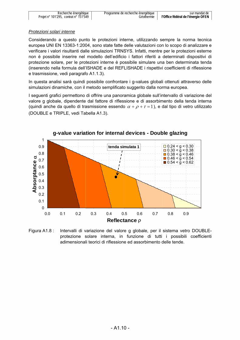
Recherche énergétique Projet n° 101’295, contrat n° 151’549
Programme de recherche énergétique Géothermie
sur mandat de l’Office fédéral de l’énergie OFEN
Protezioni solari interne
Considerando a questo punto le protezioni interne, utilizzando sempre la norma tecnica europea UNI EN 13363-1:2004, sono state fatte delle valutazioni con lo scopo di analizzare e verificare i valori risultanti dalle simulazioni TRNSYS. Infatti, mentre per le protezioni esterne non è possibile inserire nel modello dell’edificio i fattori riferiti a determinati dispositivi di protezione solare, per le protezioni interne è possibile simulare una ben determinata tenda (inserendo nella formula dell’ISHADE e del REFLISHADE i rispettivi coefficienti di riflessione e trasmissione, vedi paragrafo A1.1.3).
In questa analisi sarà quindi possibile confrontare i g-values globali ottenuti attraverso delle simulazioni dinamiche, con il metodo semplificato suggerito dalla norma europea.
I seguenti grafici permettono di offrire una panoramica globale sull’intervallo di variazione del valore g globale, dipendente dal fattore di riflessione e di assorbimento della tenda interna (quindi anche da quello di trasmissione essendo 1=++ τρα ), e dal tipo di vetro utilizzato (DOUBLE e TRIPLE, vedi Tabella A1.3).
g-value variation for internal devices - Double glazing
0
0.1
0.2
0.3
0.4
0.5
0.6
0.7
0.8
0.9
1
0.0 0.1 0.2 0.3 0.4 0.5 0.6 0.7 0.8 0.9
Reflectance ρ
Abs
orpt
ance
α
0.24 < g < 0.300.30 < g < 0.380.38 < g < 0.460.46 < g < 0.540.54 < g < 0.62
tenda simulata 1
Figura A1.8 : Intervalli di variazione del valore g globale, per il sistema vetro DOUBLE-
protezione solare interna, in funzione di tutti i possibili coefficienti adimensionali teorici di riflessione ed assorbimento delle tende.
- A1.10 -

Recherche énergétique Projet n° 101’295, contrat n° 151’549
Programme de recherche énergétique Géothermie
sur mandat de l’Office fédéral de l’énergie OFEN
g-value variation for internal devices - Triple glazing
0
0.1
0.2
0.3
0.4
0.5
0.6
0.7
0.8
0.9
1
0.0 0.1 0.2 0.3 0.4 0.5 0.6 0.7 0.8 0.9
Reflectance ρ
Abs
orpt
ance
α 0.24 < g < 0.270.27 < g < 0.300.30 < g < 0.330.33 < g < 0.360.36 < g < 0.41
tenda simulata 1
Figura A1.9 : Intervalli di variazione del valore g globale, per il sistema vetro TRIPLE-
protezione solare interna, in funzione di tutti i possibili coefficienti adimensionali teorici di riflessione ed assorbimento delle tende.
Considerando questi due ultimi grafici (Figura A1.8 e Figura A1.9) ed i precedenti (Figura A1.2 e Figura A1.3), è possibile paragonare i valori risultanti dalle simulazioni TRNSYS con quelli calcolati secondo la norma UNI EN 13363-1:2004.
Confrontando infatti i valori analizzati ed uscenti dal calcolo semplificato suggerito dalla norma europea con quelli trovati attraverso le simulazioni dinamiche che utilizzano le tre tende precedentemente descritte (vedi Tabella A1.4), si possono riscontrare risultati analoghi e concordanti per il valore g globale del sistema vetro-protezione solare interna.
Con questi due ultimi grafici è possibile inoltre valutare l’intervallo massimo di variazione del g-value; in particolare, sia per il vetro doppio che il vetro triplo analizzati, non è possibile scendere sotto lo 0.24, con alcun tipo di protezione solare interna.
Con questi due tipi di vetro, utilizzando solamente delle protezioni solari interne, non è quindi in nessun modo possibile rientrare nei vincoli imposti dalla norma SIA 382/1:2007, che impone un valore g globale comunque inferiore a 0.15.
Trasmissione solare diretta
La norma UNI EN 13363-1:2004 permette anche di determinare, per i dispositivi di protezione solare sia interni che esterni, la trasmissione solare diretta totale per l’intero sistema vetro-dispositivo di protezione solare.
Come protezione solare interna si è scelta la “tenda simulata 1” (vedi Tabella A1.4), già utilizzata nelle simulazioni dinamiche come dispositivo di protezione solare per entrambi i tipi di vetro (Figura A1.2 e Figura A1.3).
- A1.11 -

Recherche énergétique Projet n° 101’295, contrat n° 151’549
Programme de recherche énergétique Géothermie
sur mandat de l’Office fédéral de l’énergie OFEN
Mentre sulla base dei grafici rappresentati in Figura A1.6 e Figura A1.7 si è scelto, per ciascun vetro simulato, una protezione solare esterna che riesca a soddisfare i requisiti normativi della SIA 382/1:2007.
Le caratteristiche di trasmissione e riflessione solare dei due vetri sono state prese dal programma Windows5, utilizzato per la definizione dei parametri dei vetri per le simulazioni TRNSYS.
Qui di seguito sono presenti due tabelle, una per ciascun tipo di vetro, che illustrano le caratteristiche trasmissive e riflessive dei vetri e delle differenti protezioni solari, con le quali sono stati fatti i calcoli per determinare la trasmissione diretta totale.
TRIPLE glass
external device
internal device
τe 0.268 0.30 0.10 ρe, ext 0.231
ρe, int 0.231 0.50 0.45
Tabella A1.5 : Caratteristiche di trasmissione e riflessione solare del vetro TRIPLE, e dei suoi dispositivi adottati di protezione solare interni ed esterni.
DOUBLE
glass external device
internal device
τe 0.462 0.18 0.10 ρe, ext 0.237
ρe, int 0.179 0.50 0.45
Tabella A1.6 : Caratteristiche di trasmissione e riflessione solare del vetro DOUBLE, e dei suoi dispositivi adottati di protezione solare interni ed esterni.
Nella seguente Tabella A1.7 sono poi stati inseriti i valori del coefficiente g di trasmissione energetica dell’irraggiamento solare (g-value) e del grado di trasmissione diretta dell’irraggiamento solare (valore τe). I valori si riferiscono, per ciascun tipo di vetro, a quelli calcolati per una superficie vetrata senza protezioni solari, e ad una che presenta delle protezioni esterne e poi interne, in modo da valutare ed avere la sensibilità sui differenti casi.
- A1.12 -

Recherche énergétique Projet n° 101’295, contrat n° 151’549
Programme de recherche énergétique Géothermie
sur mandat de l’Office fédéral de l’énergie OFEN
global g-value τe
TRIPLE 0.41 0.27
TRIPLE + protezione esterna 0.14 0.09
TRIPLE + protezione interna 0.33 0.03
DOUBLE 0.62 0.46
DOUBLE + protezione esterna 0.14 0.11
DOUBLE + protezione interna 0.43 0.05
Tabella A1.7 : Global g-value e grado di trasmissione diretta dell’irraggiamento solare τe per i vetri senza e con le protezioni solari interne o esterne.
- A1.13 -

Recherche énergétique Projet n° 101’295, contrat n° 151’549
Programme de recherche énergétique Géothermie
sur mandat de l’Office fédéral de l’énergie OFEN
A1.1.5. Guadagni interni I guadagni interni sono definiti sulla base delle indicazioni contenute nel quaderno tecnico SIA 2024 per la categoria “grande ufficio”. I guadagni considerati sono: da persone (people), da illuminazione (lighting) e da apparecchiature elettriche (appliances).
In Figura A1.10 sono mostrati i profili giornalieri dei guadagni interni per i giorni lavorativi. I guadagni sono definiti per metro quadrato di superficie interna (corrisponde a circa l’85% della superficie di riferimento energetico (SRE), definita secondo la norma SIA 380/1 (2009). I profili sono stati definiti mantenendo i valori di picco indicati nel quaderno tecnico SIA 2024 (concentrati nelle prime ore del pomeriggio per creare delle condizioni di simulazione cautelative rispetto al surriscaldamento estivo) e l’integrale dei carichi su base annua (energia ceduta all’ambiente interno per m2 di superficie).
Sulla base del profilo di un giorno lavorativo tipo, i guadagni interni totali (total) possono raggiungere un valore massimo pari a 26.1 W/m2.
In termini di media annuale, i guadagni interni corrispondono a 1 W/m2 per le persone, 3.3 W/m2 per l’illuminazione e 1.7 W/m2 per le apparecchiature, ovvero a 0.85 W/m2 per le persone, 2.8 W/m2 per l’illuminazione e 1.45 W/m2 per le apparecchiature, se si considera la superficie di riferimento energetico (SRE) secondo la SIA 380 (2009).
I guadagni interni, corrispondenti a mediamente 6 W/m2 relativamente alla superficie interna, o a 5.1 W/m2 relativamente alla SRE, sono superiori rispetto a quelli previsti dalla norma SIA 380/1, in quanto in quest’ultimo le condizioni d’utilizzo sono definite in relazione a tutto l’edificio, e comprende anche utilizzi spaziali come per esempio sala riunione, atrio sportelli, WC e spazio di circolazione. Secondo la norma SIA 380/1 i guadagni interni ammontano, relativamente alla SRE, a 3.3 W/m2, di cui 1 W/m2 per i guadagni attribuiti alle persone e 2.3 W/m2 ai guadagni termici risultanti dai consumi elettrici.
- A1.14 -

Recherche énergétique Projet n° 101’295, contrat n° 151’549
Programme de recherche énergétique Géothermie
sur mandat de l’Office fédéral de l’énergie OFEN
Giorno lavorativo (lunedì - venerdì)
0
5
10
15
20
25
30
0:00 4:00 8:00 12:00 16:00 20:00 0:00Ore del giorno [hh:mm]
Gua
dagn
i int
erni
[W/m
2]
totallightingappliancespeople
Figura A1.10 : Profilo dei guadagni interni per un giorno lavorativo (lunedì – venerdì). La
superficie di riferimento è quella interna, posta pari all’85% della SRE, la superficie di riferimento energetico.
Il profilo dei guadagni interni per il fine settimana (sabato – domenica) è dato solo dallo stand-by delle apparecchiature, come da quaderno tecnico SIA 2024. Ciò corrisponde a 0.8 W/m2 costanti, se si considera la superficie interna o a 0.68 W/m2 se si considera la SRE.
A1.1.6. Ventilazione Il ricambio d’aria è definito sulla base di due componenti:
- ricambio d’aria dovuto alle infiltrazioni. Si assume un ricambio costante pari a 0.1 [h-1];
- ricambio d’aria vero e proprio, dato dall’impianto di ventilazione meccanica. Si assume un ricambio costante pari a 0.5 [h-1] dalle 8:00 alle 18:00 per tutti i giorni dell’anno. Per ovvie ragioni di efficienza energetica, si assume un recupero di calore mediante uno scambiatore aria-aria caratterizzato da un’efficienza pari all’ 80%.
Inoltre, durante l’estate, se le condizioni lo permettono, è possibile effettuare un raffrescamento notturno dalle 22:00 alle 6:00 con un ricambio d’aria di 2 [h-1].
- A1.15 -
Recherche énergétique Projet n° 101’295, contrat n° 151’549
Programme de recherche énergétique Géothermie
sur mandat de l’Office fédéral de l’énergie OFEN
Sulla base delle precedenti assunzioni, si ha un ricambio d’aria medio durante il periodo di riscaldamento corrispondente a 0.31 [h-1], con 0.1 [h-1] per le infiltrazioni e 0.21 [h-1] per la ventilazione meccanica.
La norma SIA 380/1 fissa un valore pari a 0.7 m3/h /m2 , al quale corrisponde un tasso di ricambio dell’aria di 0.27 [h-1] (SRE = 2'200 m2 e volume riscaldato netto di 5'700 m3). Il ricambio di aria dell’edificio simulato è quindi leggermente più elevato di quello fissato dalla norma SIA 380/1.
A1.1.7. Capacità termica interna La capacità termica dell’edificio è simulata con le solette interne, le pareti massive dell’involucro dell’edificio (interne ed esterne) ed una capacità termica istantanea fissata a 14.6 Wh/m2K in riferimento alla SRE, valore considerato realistico sulla base di simulazioni precedentemente condotte (la capacità termica totale dell’edificio così simulata consente variazioni di temperatura giornaliere dell’ordine di 3 K, compatibili con edifici di questo tipo).
Come caso di riferimento è stato assunto un edificio di capacità termica media come da quaderno tecnico 2024, ovvero caratterizzato da una capacità termica pari a 150 Wh/m2K (in riferimento alla superficie interna).
Le caratteristiche corrispondenti sono :
- capacità termica istantanea : 14.6 Wh/m2K
- capacità termica da pareti interne : 22.9 Wh/m2K
- capacità termica da pareti esterne opache (50% superfici facciate) e solette : 112.5 Wh/m2K
A1.2. Riferimenti
Klein S. A. et al. (2007) TRNSYS. A Transient System Simulation Program. Version 16.1. Solar Energy Laboratory, University of Wisconsin, Madison, USA.
Merkblatt SIA 2024 (2006) Standard-Nutzungsbedingungen für die Energie- und Gebäudetechnik. Schweizerischer Ingenieur- und Architektenverein, Zürich, Schweiz.
Pahud D., Caputo P., Branca G. Et Generelli M. (2008) Etude du potentiel d’utilisation de geocooling d’une installation avec sondes géothermiques verticales appliqué à un bâtiment administratif Minergie® à Chiasso. Rapport final, Office fédéral de l’énergie, Berne, Suisse.
SIA 380/1 (2009) L'energia termica nell'edilizia. Società Svizzera degli Ingegneri e degli Architetti, Zurigo, Svizzera.
SIA 382/1 (2007) Lüftungs- und Klimaanlagen – Allgemeine Grundlagen und Anforderungen. Schweizerischer Ingenieur- und Architektenverein, Zürich, Schweiz.
UNI EN 13363-1 (2004) Solar protection devices combined with glazing – Calculation of solar and light transmittance – Simplified method. Ente Nazionale Italiano di Unificazione, Milano, Italia.
Windows 5.0 (2001) A PC Program for Analyzing Window Thermal Performance. User Manual. Lawrence Berkeley National Laboratory, Berkeley, USA.
- A1.16 -
Manuale per il raffreddamento di edifici tramite « geocooling » con sonde geotermiche verticali
Annex 2
Simulation model of the building and ground coupled system
Indice A2.1. The simulation software 1 A2.2. The building model 1 A2.3. The ground coupled model 3 A2.4. The system simulation tool 4 A2.5. References 4
Rapporto finale D. Pahud e M. Belliardi


Recherche énergétique Projet n° 101’295, contrat n° 151’549
Programme de recherche énergétique Géothermie
sur mandat de l’Office fédéral de l’énergie OFEN
A2.1. The simulation software
As described in chapter 4, the system simulation programme of transient thermal processes TRNSYS (Klein and al., 2007) is chosen for the simulation of the building, the heating and cooling energy distribution, the technical installations and the borehole heat exchangers. TRNSYS version 16.1 is used.
A2.2. The building model
A reference office building is chosen for the study, as well as a reference location for climatic data. The recent office building of the Brogeda custom in Chiasso (Tessin, Switzerland) is selected for the definition of the reference building (see Annex 1). The building complies to the low energy Minergie® standard. Heating and cooling energy is distributed through active concrete plates, which makes possible low heating and high cooling temperatures, and enables auto-regulating properties. A2.2.1. Building thermal zones The building, simulated with the TRNSYS standard type TYPE56, is divided into two thermal zones (see chapter 4 for more details). The first zone is a single room below the roof, which gives the possibility to study thermal comfort issues under particular conditions. The second zones is the rest of the building, so that the global overall energy requirements of the whole building are simulated and known for the ground coupled system. Four additional fictive zones are defined for the simulation of the heating and cooling distribution system. They represent the average concrete temperature in the plane of the imbedded pipes, i.e. in the middle plane of the active concrete plates. The four fictive zones enable to take into consideration the various boundary conditions of the active concrete plates, such as ceiling or pavement to zone 1 or 2, or outdoor insulated roof. In this way the computation of the thermal process is divided in two parts: - heat transfers in the massive structure over and below the pipe plane are simulated in TYPE56, taking into account heat capacitive effects and boundary conditions; - heat transfer from the circulating fluid in the distribution system and the average concrete temperature in the pipe plane is simulated on the basis of the formalism developed by Koschenz and Dorrer (1996), using the practical method proposed by Pahud and al. (2000), which is based on heat exchanger heat transfer. The heat rate transfer is calculated outside of TYPE56, on the basis of the forward fluid temperature in the pipe flow circuit, the fluid flow rate and the mean concrete temperature in the pipe plane. It is then given as an input variable to TYPE56 as a heat gain in the corresponding fictive zone. Solutions are found by iterations thanks to the TRNSYS solver engine. In the TAB case heating and cooling is primarily emitted through ceiling, as a technical pavement is supposed to lie on the floor. In the PAV case this is the other way round, i.e. heating and cooling emission through floors as a technical space is supposed to be present at the ceiling between concrete plate and room.
- A2.1 -

Recherche énergétique Projet n° 101’295, contrat n° 151’549
Programme de recherche énergétique Géothermie
sur mandat de l’Office fédéral de l’énergie OFEN
In Figure A2.1 the location of the thermal zones are shown for the TAB case, i.e. heating and cooling with active concrete plates.
Zone 1: AULAZone 2: UFFICI
Zone 2: UFFICI
Zone 3: TAB 1Zone 4: TAB 2 Zone 4: TAB 2
Zone 5: TAB 3
Zone 6: TAB 4
Zone 1: AULAZone 2: UFFICI
Zone 2: UFFICI
Zone 3: TAB 1Zone 4: TAB 2 Zone 4: TAB 2
Zone 5: TAB 3
Zone 6: TAB 4
Zone 1: AULAZone 2: UFFICI
Zone 2: UFFICI
Zone 3: TAB 1Zone 4: TAB 2 Zone 4: TAB 2
Zone 5: TAB 3
Zone 6: TAB 4
Figure A2.1 Location of the zones for the TAB case. Zone 1 “AULA” is a room at the last
floor under the roof. Zone 2 “UFFICI” is defined for the rest of the heated and cooled building. Zones 3 to 6 are defined for the simulation of the active concrete plates. Heating and cooling requirements are distributed through ceilings.
In Figure A2.2 the location of the fictive zones are shown for the PAV case, i.e. heating and cooling with floors.
Zone 1: AULAZone 2: UFFICI
Zone 2: UFFICI
Zone 3: PAV 1Zone 4: PAV 2 Zone 4: PAV 2
Zone 5: PAV 3
Zone 6: PAV 4
Zone 1: AULAZone 2: UFFICI
Zone 2: UFFICI
Zone 3: PAV 1Zone 4: PAV 2 Zone 4: PAV 2
Zone 5: PAV 3
Zone 6: PAV 4
Figure A2.2 Location of the zones for the case PAV. Zones 3 to 6 are defined for the
simulation of the heating and cooling distribution through the floors.
- A2.2 -

Recherche énergétique Projet n° 101’295, contrat n° 151’549
Programme de recherche énergétique Géothermie
sur mandat de l’Office fédéral de l’énergie OFEN
In the PAV case the number of zones for the simulation of the heating and cooling floors is not reduced from 4 to 2, so that the same building model structure can be used for both TAB and PAV case. In this way the number of INPUTS and OUTPUTS for TYPE56 is equal for both cases. All the necessary parameters for the building definition are contained in a file that is read by TYPE56. This file is generated by the TRNBuild programme of the TRNSYS16.1 package (see annex 3 for a description of the building inputs and outputs). The analysis of the heat distribution (TAB or PAV), the glazing (TRIPLE or DOUBLE) and the glazing ratio (50% or 85%) required to change the building definition file. As a result 8 different building files were created. Solar protections (external or internal), the magnitude of the internal heat gains, building façade orientation and air change rate magnitude are controlled in the TRNSYS deck, i.e. outside of the building definition file.
A2.3. The ground coupled model
The ground coupled system is simulated with PILESIM (Pahud, 2007). It does include the borehole heat exchangers model, the simulation of the horizontal pipe connections between boreholes and distributors, and, if relevant, the interface between ground and building. A heat pump model for heating and a flat plate counter flow heat exchanger for geocooling are also included in the system simulation. The representation of the macro created for PILESIM in the Simulation Studio of the TRNSYS package is shown in figure A2.3.
Figure A2.3 Macro “PILESIM” created in the Simulation Studio of the TRNSYS package. The
macro “PILESIM” uses the macro “TRNVDSTP-with-PIPES”. This macro contains the TRNVDSTP TYPE with some other TRNSYS TYPES such as pipe components to take into account the thermal heat transfer of the horizontal pipe connections at ground surface.
- A2.3 -
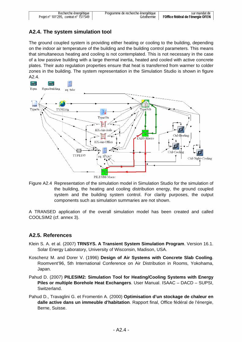
Recherche énergétique Projet n° 101’295, contrat n° 151’549
Programme de recherche énergétique Géothermie
sur mandat de l’Office fédéral de l’énergie OFEN
A2.4. The system simulation tool
The ground coupled system is providing either heating or cooling to the building, depending on the indoor air temperature of the building and the building control parameters. This means that simultaneous heating and cooling is not contemplated. This is not necessary in the case of a low passive building with a large thermal inertia, heated and cooled with active concrete plates. Their auto regulation properties ensure that heat is transferred from warmer to colder zones in the building. The system representation in the Simulation Studio is shown in figure A2.4.
Figure A2.4 Representation of the simulation model in Simulation Studio for the simulation of
the building, the heating and cooling distribution energy, the ground coupled system and the building system control. For clarity purposes, the output components such as simulation summaries are not shown.
A TRANSED application of the overall simulation model has been created and called COOLSIM2 (cf. annex 3).
A2.5. References Klein S. A. et al. (2007) TRNSYS. A Transient System Simulation Program. Version 16.1.
Solar Energy Laboratory, University of Wisconsin, Madison, USA.
Koschenz M. and Dorer V. (1996) Design of Air Systems with Concrete Slab Cooling. Roomvent’96, 5th International Conference on Air Distribution in Rooms, Yokohama, Japan.
Pahud D. (2007) PILESIM2: Simulation Tool for Heating/Cooling Systems with Energy Piles or multiple Borehole Heat Exchangers. User Manual. ISAAC – DACD – SUPSI, Switzerland.
Pahud D., Travaglini G. et Fromentin A. (2000) Optimisation d’un stockage de chaleur en dalle active dans un immeuble d’habitation. Rapport final, Office fédéral de l’énergie, Berne, Suisse.
- A2.4 -

Manuale per il raffreddamento di edifici tramite « geocooling » con sonde geotermiche verticali
Rapporto finale D. Pahud e M. Belliardi
Annex 3
The COOLSIM2 simulation tool
Table of content A3.1. The COOLSIM2 Simulation Tool 1
A3.1.1. Introduction 1 A3.1.2. COOLSIM2 System Border 1 A3.1.3. BUISIM System Border 2 A3.1.4. COOLSIM2 System Simulation Tool 2 A3.1.5. Input Data to COOLSIM2 3 A3.1.6. How to Run COOLSIM2 20 A3.1.7. Output Data from COOLSIM2 23 A3.1.8. Output Results with COOLSIM2 32
A3.2. Input parameters for the building 39 A3.2.1. Introduction 39 A3.2.2. INPUT variables 39 A3.2.3. OUTPUT variables 40 A3.2.4. Tips for the building model definition 41
A3.3. References 51


Recherche énergétique Projet n° 101’295, contrat n° 151’549
Programme de recherche énergétique Géothermie
sur mandat de l’Office fédéral de l’énergie OFEN
- A3.1 -
A3.1. The COOLSIM2 Simulation Tool
A3.1.1. Introduction The COOLSIM2 simulation tool is devised for the simulation of office buildings heated with a heat pump coupled to a borehole field or energy piles, and cooled with these latter by geocooling. No hot water is covered by the system. The energy concept involves a heat pump directly coupled to active concrete plates (TAB) or floor heating (PAV), which are also used for cooling. The whole building is either heated or cooled. It is assumed that auto-regulating properties of the heat and cold emitters are sufficient to ensure heat transport from warmer to colder parts of the building. No cooling and dehumidification is simulated in the building ventilation system. Air change rate is fixed for hygienic purposes only. It is assumed that quasi the totality of thermal energy is conveyed through the water distribution system. The COOLSIM2 simulation tool has been developed on the basis of the PILESIM2 simulation tool (PAHUD, 2007) in TRNSYS 16.1 environment. A3.1.2. COOLSIM2 System Border The delimitation of the simulated system is shown by the system border in figure A3.1.
Figure A3.1 System simulated by the COOLSIM2 tool.
System border
Ground layer 1
Ground layer 2
Ground layer 3
Energy piles orborehole heat exchangers
Cellar Heat pump
Cold distributionHeat distributionHeated / cooled building
System border
Ground layer 1
Ground layer 2
Ground layer 3
Energy piles orborehole heat exchangers
Cellar Heat pump
Cold distributionHeat distributionHeated / cooled building

Recherche énergétique Projet n° 101’295, contrat n° 151’549
Programme de recherche énergétique Géothermie
sur mandat de l’Office fédéral de l’énergie OFEN
- A3.2 -
A3.1.3. BUISIM System Border In a first step the heating and cooling requirements of the building are determined with the TRANSED input file BUISIM.TRD. In this file the geothermal system is excluded from the simulation. The delimitation of the system simulated with BUISIM is shown in figure A3.2.
Figure A3.2 System part simulated by the BUISIM tool. A3.1.4. COOLSIM2 System Simulation Tool The use of COOLSIM2 requires to define first the heating and cooling requirements of the building. Heating power and cooling temperature have to be adjusted together with set point temperatures and controls, so that thermal comfort is ensured with minimum energy requirements. The TRANSED input file BUISIM.TRD has been devised for this purpose. It is a simplified version of the input file COOLSIM.TRD. The input data to BUISIM.TRD are the same as those for COOLSIM.TRD, except for the non necessary components, such as the geothermal system, whose parameters have been set to exclude them from a simulation. A procedure has been developed to define all the necessary parameters in BUISIM, i.e. all parameters related to building use and control (see annex 4). In next section, input data to the COOLSIM2 programme are listed and defined.
System border for the determination of heating and cooling parameters (TabSim)
Ground layer 1
Ground layer 2
Ground layer 3
Energy piles orborehole heat exchangers
Cellar Heat pump
Cold distributionHeat distributionHeated / cooled building
System border for the determination of heating and cooling parameters (TabSim)
Ground layer 1
Ground layer 2
Ground layer 3
Energy piles orborehole heat exchangers
Cellar Heat pump
Cold distributionHeat distributionHeated / cooled building

Recherche énergétique Projet n° 101’295, contrat n° 151’549
Programme de recherche énergétique Géothermie
sur mandat de l’Office fédéral de l’énergie OFEN
- A3.3 -
A3.1.5. Input Data to COOLSIM2 The input data to COOLSIM2 concern all the information that can be varied by the user. In particular, the input data define the size and characteristics of the different parts of the system and the driving conditions which will condition the operation of the system. In this chapter, each parameter that can be adjusted in COOLSIM2 is described and explained. The input data are grouped in 6 blocks presented in various tabs: • Simulation and location • Building • Heating and cooling • Interface ground-building • Ground heat exchanger • Ground characteristics The BUISIM tool, used to determine the building control, heating and cooling requirements, only requires the input data of the three tabs “Simulation and location”, “Building” and “Heating and cooling”. COOLSIM2 and BUISIM are TRNSED applications. The input parameter values may either be given in “primary units”, which correspond to the unit assumed by TRNSYS, or in “secondary units”, which are more convenient units for the user. For example, primary unit of thermal conductivity is [kJ/(h m K)], whereas secondary unit is [W/(mK)]. All the units given for the input parameters in the following sections correspond to “secondary units”. When COOLSIM2 or BUISIM is used, it is highly recommended to set the units on “secondary”. This is done by selecting Secondary Units in the menu TRNSYS of the TRNSED application. The Simulation and location tab: The entries are grouped in three blocks: Simulation parameters (in tab “Simulation and location”) Month for simulation start: the simulation starts the first day of the chosen month. Length of simulation: duration of the simulation period. The maximum duration is limited to
50 years. Time interval for output results: quantities can be calculated on a monthly basis or a
yearly basis. They are integrated heat rates or average values. See chapter A3.1.8 for a complete description of the output results.
Print hourly values for last year: this parameter determines if the hourly values of some
selected quantities are written (yes) or not (no) for the last operational year (see chapter A3.1.8 for more details).

Recherche énergétique Projet n° 101’295, contrat n° 151’549
Programme de recherche énergétique Géothermie
sur mandat de l’Office fédéral de l’énergie OFEN
- A3.4 -
Online plotter (in tab “Simulation and location”) Check the box to plot thermal powers and fluid temperatures of the ground heat system
during simulation. Location parameters (in tab “Simulation and location”) Meteorological data for location: choose from the list the location of the project. This
choice determines the weather data file that will be used for the simulation. If you would like to add more locations, you have to create a weather file with Meteonorm and update the file LocationList.txt in the Weather subdirectory. Please follow the indications given in this file.
Latitude, longitude and altitude of location: choose from the list the same location of the
previous one used for the meteorological data. This choice sets the latitude, longitude and altitude of the location.
The Building tab: Building parameters (in tab “Building”) Data file for building description: choose from the list the building name to be simulated.
This choice determines the building data file that defines the building thermal parameters. If you would like to add more buildings, you have to define them with TRNBuild of the TRNSYS package and update the file BuildingList.txt in the Building subdirectory. Please follow the indications given in this file.
Surface values for building data file: choose from the list the same building name as the
previous one. This choice sets various surface areas. They are: - SRE: heated/cooled reference area of building (zone 1 and 2) [m2] - Stabs3: area of the fictive zone 3 used for the simulation of TAB3 or PAV3 [m2] - Stabs4: area of the fictive zone 4 used for the simulation of TAB4 or PAV4 [m2] - Stabs5: area of the fictive zone 5 used for the simulation of TAB5 or PAV5 [m2] - Stabs6: area of the fictive zone 6 used for the simulation of TAB6 or PAV6 [m2] The total area of the TAB or PAV in the building is given by the sum of the areas of the 4
fictive zones (zone 3 to 6). These latter are stored in the file BuildingList.txt and must correspond to the building description file. Please follow the indications given in this file for any modification.
Azimuth of south façade [AzimSud]: azimuth of the south façade [°]. Should be comprised
between -45° and +45° (azimuth south-east: -45°, south: 0°, south-west: +45°). All the 4 façades are supposed to be at right angle, forming thus a rectangular shape.
Scaling factor for internal heat gains [ScaleGainInt]: scaling factor for internal heat gains
[-]. The daily and weekly profile of the internal heat gains are defined in the building definition file. This scaling factor enable to amplify them with a constant factor.
Air change rate for night cooling [ACRnight]: air change rate for nocturnal ventilation
when the building is cooled during Summer. A typical value is an air change rate of 2 [h-1]. Nocturnal ventilation is only performed if the following conditions are met:
- the outdoor air temperature is lower than the indoor air temperature; - night operation is allowed by the NOTTE schedule in the building definition file (see
section A3.2.4 – SCHEDULE TYPES). In the reference building the time window is set between 22h and 6h;

Recherche énergétique Projet n° 101’295, contrat n° 151’549
Programme de recherche énergétique Géothermie
sur mandat de l’Office fédéral de l’énergie OFEN
- A3.5 -
- and the running mean outdoor air temperature, defined according to the standard DIN
EN 15251, is greater than 15°C. Nominal air change rate of mechanical system ventilation [ACRmechanic]: nominal air
change rate of the mechanical system ventilation [h-1]. The mechanical system ventilation is operating according to the daily schedule V_05_ONOFF defined in the building definition file (see section A3.2.4 – SCHEDULE TYPES). In the reference building the operation time window is set between 8h and 18h. When the ventilation system is operating, this parameter defines the ventilation air change rate.
Efficiency of the mechanical system heat recovery units [AirHXEfficiency]: nominal
efficiency of the mechanical system heat recovery units [-]. The heat recovery units of the mechanical ventilation system are simulated with a constant heat exchanger efficiency. A typical value is an efficiency of 0.8 [-]
Specific flow rate in TABS [FlowSpecTABS]: specific flow rate in tabs [(kg/h)/m2]. It is the
total flow rate through the TABS divided by the total area of the concrete active plates; (it is the area of all the internal concrete plates equipped with pipes).
Thermal resistance fluid-concrete in TABS [RTABS]: thermal resistance between the fluid
circulating in the pipes and the concrete in the plane of the pipes [K/(W/m2)].
⎟⎟⎠
⎞⎜⎜⎝
⎛⎟⎠⎞
⎜⎝⎛+⎟
⎟⎠
⎞⎜⎜⎝
⎛+=
πδλπδδ
λπλπ ln
2 ln
2
Nu RTABS
pip f
ll
111 (A3.1)
With : l : distance between pipes in the concrete plates (typical distance = 0.15 [m] ) (TABS); λf : thermal conductivity of the fluid circulating in the pipes (water = 0.6 [W/mK] ); Nu : Nusselt number for the convective heat transfer between fluid and inner pipe wall. It
depends on the fluid flow regime (laminar, Nu = 4.36 [-] ); λp : thermal conductivity of the pipe material (plastic pipe in polyethylene: 0.4 [W/mK] ); λ : concrete plate thermal conductivity (concrete : 1.8 [W/mK] ); δ : external pipe diameter (typical diameter = 0.02 [m] ); δpi : internal pipe diameter (typical diameter = 0.016 [m] ); RTABS : thermal resistance between the fluid temperature and mean concrete
temperature in the pipe plane (RTABS is calculated to 0.043 [K/(W/m2)] with above parameters);
The validity of equation (A3.1) is guaranteed if the following two conditions are met :
2 and 1i , .3 / di => 0l (A3.2)
.2 / 0<lδ (A3.3) d1+d2 : concrete plate thickness [m] ; d1 : thickness of concrete plate layer lying over the pipe plane [m] ; d2 : thickness of concrete plate layer lying under the pipe plane [m] .

Recherche énergétique Projet n° 101’295, contrat n° 151’549
Programme de recherche énergétique Géothermie
sur mandat de l’Office fédéral de l’énergie OFEN
- A3.6 -
Solar protections (in tab “Building”) Select between: • No solar protections : solar protections are not simulated • Solar protections : solar protections are simulated and the parameters in the next
box (Solar protections parameters) have to be defined Solar protections parameters (in tab “Building”) This box is visible only if option “• Solar protections” is selected in the previous box Vertical global solar radiation limit to use solar protections in Winter [IvLimitWinter]:
Winter vertical global solar radiation threshold over which solar protections are used [W/m2]. Under the radiation threshold the solar protections are not screening or limiting the passive solar gains. This radiation threshold is used during the Winter period, defined as the period of the year when cooling is not allowed (see parameter TlimitSummer "Daily temperature limit to allow cooling operation" in the next box (Building control parameters)). When global radiation in one of the building façade is exceeding the Winter radiation threshold, the solar protections are used as defined with the next two parameters (IShadeWinter and EShadeWinter).
Internal shading device efficiency in Winter (0: no shading, 1-Tau: maximal shading)
[IShadeWinter]: average shading factor of the internal solar protections when cooling is not allowed (0: no shading, 1-Tau: maximal shading; Tau is the shading device transmission coefficient). This shading factor is applied simultaneously on all windows of all façades of the building.
External shading device efficiency in Winter (0: no shading, 1: maximal shading)
[EShadeWinter]: average shading factor of the external solar protections when cooling is not allowed (0: no shading, 1: maximal shading). This shading factor is applied simultaneously on all windows of all façades of the building.
Vertical global solar radiation limit to use solar protections in Summer
[IvLimitSummer]: Summer vertical global solar radiation threshold over which solar protections are used [W/m2]. Under the radiation threshold the solar protections are not screening or limiting the passive solar gains. This radiation threshold is used during the Summer period, defined as the period of the year when cooling is allowed (see parameter TlimitSummer "Daily temperature limit to allow cooling operation" in the next box (Building control parameters)). When global radiation in one of the building façade is exceeding the Summer radiation threshold, the solar protections are used as defined with the next two parameters (IShadeSummer and EShadeSummer).
Internal shading device efficiency in Summer (0: no shading, 1-Tau: maximal shading)
[IShadeSummer]: average shading factor of the internal solar protections when cooling is allowed (0: no shading, 1-Tau: maximal shading; Tau is the shading device transmission coefficient). This shading factor is applied simultaneously on all windows of all façades of the building.
External shading device efficiency in Summer (0: no shading, 1: maximal shading)
[EShadeSummer]: average shading factor of the external solar protections when cooling is allowed (0: no shading, 1: maximal shading). This shading factor is applied simultaneously on all windows of all façades of the building.

Recherche énergétique Projet n° 101’295, contrat n° 151’549
Programme de recherche énergétique Géothermie
sur mandat de l’Office fédéral de l’énergie OFEN
- A3.7 -
Building control parameters (in tab “Building”) Daily temperature limit to control heat recovery operation [TlimitVentHX]: daily outdoor
air temperature limit under which heat recovery on the ventilation system is performed [°C]. The running mean outdoor air temperature, defined according to the standard DIN EN 15251, is chosen for the daily outdoor air temperature. It has no direct influence on the heating control of the building.
Daily temperature limit to allow cooling operation [TlimitSummer]: daily outdoor air
temperature limit over which cooling is allowed [°C]. The running mean outdoor air temperature, defined according to the standard DIN EN 15251, is chosen for the daily outdoor air temperature. This temperature condition has to be met to enable the cooling control of the building and nocturnal cooling with the ventilation system. It is used to determine the duration of the cooling period. The remaining time of the year is the winter use duration. In any case cooling is only allowed if no heating requirement is requested. In practice heating and cooling conflict never happens as it is requested that the indoor air temperature limit to switch off cooling (TSetCoolingLow) is larger than that to switch off heating (TSetHeatingHigh).
Set point temperature to switch on heating [TSetHeatingLow]: indoor air temperature
limit under which heating is switched on [°C]. Heating is only allowed if the running mean outdoor air temperature, defined according to the standard DIN EN 15251, is lower than 15°C. If the heating distribution is not simulated, i.e. case with a fixed minimum indoor air temperature in BUISIM, this parameter is ignored and has no influence on the heating demand.
Set point temperature to switch off heating [TSetHeatingHigh]: indoor air temperature
limit over which heating is switched off [°C]. This temperature limit has to be larger than TSetHeatingLow, used to switch on heating. Heating is only allowed if the running mean outdoor air temperature, defined according to the standard DIN EN 15251, is lower than 15°C. If the heating distribution is not simulated, i.e. case with a fixed minimum indoor air temperature in BUISIM, this parameter is ignored and has no influence on the heating demand.
Set point temperature to switch on cooling [TSetCoolingHigh]: indoor air temperature
limit over which cooling is switched on [°C]. If the cooling distribution is not simulated, i.e. case with a fixed maximum indoor air temperature in BUISIM, this parameter is ignored and has no influence on the cooling demand.
Set point temperature to switch off cooling [TSetCoolingLow]: indoor air temperature
limit under which cooling is switched off [°C]. This temperature limit has to be smaller than TSetCoolingHigh, used to switch on cooling. If the cooling distribution is not simulated, i.e. case with a fixed maximum indoor air temperature in BUISIM, this parameter is ignored and has no influence on the cooling demand.

Recherche énergétique Projet n° 101’295, contrat n° 151’549
Programme de recherche énergétique Géothermie
sur mandat de l’Office fédéral de l’énergie OFEN
- A3.8 -
The Heating and cooling tab: Heat pump power and efficiency (in tab “Heating and cooling”) Design thermal power of the heat pump [PHeatDesign]: design (or nominal) thermal
power delivered at the condenser of the heat pump (PAC). It is the heating power delivered by the heat pump at nominal temperature conditions in evaporator and condenser [kW].
Design performance coefficient [COPo]: the design performance coefficient is the
performance coefficient of the heat pump when the inlet fluid temperature in the evaporator and the outlet fluid temperature from the condenser are at their design values [-]. The design performance coefficient is expressed by relation (A3.4):
COPo = PHeatDesign / Pel (A3.4)
PHeatDesign: design heating power delivered by the heat pump. Pel: design electric power absorbed by the compressor of the heat pump. The design electric power of the heat pump is assumed to be constant even when the heat pump performance coefficient is calculated in function of the temperature levels in evaporator and condenser. Heat pump COP (in tab “Heating and cooling”) Select between: • Constant COP during simulation : the performance coefficient is kept constant and
set to its design value (COPo) during a simulation
• Variable COP during simulation : the performance coefficient is free to vary according to operating conditions during a simulation
Heat pump COP dependencies (in tab “Heating and cooling”) This box is visible only if option “• Variable COP during simulation” is selected in the previous box. The parameters for the heat pump COP dependencies refer to the heat pump model described in chapter 7 of the PILESIM2 user manual (Pahud, 2007). Design inlet fluid temperature in evaporator for COPo: design inlet fluid temperature in
the evaporator that leads to the design performance coefficient (COPo) of the heat pump [°C].
Design outlet fluid temperature from condenser for COPo: design outlet fluid
temperature from the condenser that leads to the design performance coefficient (COPo) of the heat pump [°C].
Temperature difference for COP reduction: parameter dTCOP for the heat pump model
[K]. See the PILESIM2 user manual (Pahud, 2007) for more details. Temperature difference for COP stagnation: parameter dTstag for the heat pump model
[K]. See the PILESIM2 user manual (Pahud, 2007) for more details.

Recherche énergétique Projet n° 101’295, contrat n° 151’549
Programme de recherche énergétique Géothermie
sur mandat de l’Office fédéral de l’énergie OFEN
- A3.9 -
Maximum possible COP: maximum value that the heat pump performance coefficient
(COP) may have [-]. Penalty on the COP: penalty on the performance coefficient [-]. This value is subtracted
from the calculated value, so that transient effects, bad control of the heat pump or something else, can be artificially taken into account. Typical values are comprised between 0 and 0.5.
Heat pump temperature difference (in tab “Heating and cooling”) Design inlet-outlet temperature difference in evaporator (PAC): design temperature drop
between inlet and outlet fluid that crosses the heat pump evaporator [K]. Together with the heat power extracted under design conditions, this temperature drop determines the flow rate through the evaporator. This flow rate is also the total flow rate in the flow circuit of the borehole heat exchangers or the energy piles when the heat pump is operating. It is called the heating flow rate. When the operating mode is geocooling, the flow rate through the pile flow circuit is equal to that in the cooling distribution of the building, even if a heat exchanger is physically decoupling hydraulically the two flow circuits.
Design inlet-outlet temperature difference in condenser (PAC): design temperature drop
between inlet and outlet fluid that crosses the heat pump condenser [K]. This temperature difference, together with the design thermal power of the heat pump, is determining the fluid flow rate through the heat pump condenser. It is important that the flow rate through the heat distribution system (TAB or else) is not smaller than the flow rate through the heat pump condenser. If it is the case, the flow rate in the distribution system is set to the heat pump condenser flow rate when heating is performed.
Temperature limitation (in tab “Heating and cooling”) Minimum allowed temperature of the heat carrier fluid in the piles/boreholes [TfMin]:
minimum tolerated fluid temperature in the bores/piles hydraulic circuit [°C]. This value may limit the heat rate that is extracted from the ground, as the simulated inlet fluid temperature in the bores / piles is limited by this value. This constraint limits the size of the heat pump or the total length of the borehole heat exchangers, as a normal system operation should never lead to a fluid temperature below this limit. It is recommended not to use this temperature limitation for the sizing of the system (set TfMin to -50°C). The system should be sized so that the fluid temperature never drops below the minimum allowed fluid temperature during a whole simulation.

Recherche énergétique Projet n° 101’295, contrat n° 151’549
Programme de recherche énergétique Géothermie
sur mandat de l’Office fédéral de l’énergie OFEN
- A3.10 -
Geocooling (in tab “Heating and cooling”) Design forward fluid temperature for cooling [TCoolDesign]: design forward fluid
temperature for cooling [°C]. This value is assumed to be constant all through the year. If the outlet fluid temperature from the ground heat exchanger is low enough to guarantee this forward fluid temperature (taking into account the counter flow heat exchanger between the cooling distribution and the ground flow loop), then the cooling requirement is met. The forward fluid temperature in the cooling distribution is fixed to the design one (TCoolDesign). If the resulting temperature lies between the design forward one and the return fluid temperature from the cooling distribution, then only a fraction of the cooling demand is met. If the resulting temperature is larger than the return one from the cooling distribution, geocooling is not possible and stopped. In this case the cooling demand is not satisfied. No backup cooling energy is provided in the building. It will result a larger indoor air temperature and a lesser thermal comfort in the building.
Design heat transfer coefficient of geocooling counterflow heat exchanger
[HXUAGEO]: design heat transfer coefficient of the counterflow heat exchanger between the cooling distribution and the ground flow loop [kW/K]. If no heat exchanger is present, this parameter can be fixed to an arbitrary large value (for example 1025 kW/K).
The Interface ground-building tab: Location of the ground heat exchanger (in tab “Interface ground-building”) Select between: • energy piles, borehole heat exchangers under the building: the ground heat
exchanger is located under the building. The corresponding parameters are shown in next box, which is called “Interface ground heat exchanger-building”
• borehole heat exchangers outside of the building: the ground heat exchanger is located outside of the building. The corresponding parameters are shown in next box, which is called “Interface building-ground and ground heat exchanger-garage”
Interface ground heat exchanger-building (in tab “Interface ground-building”) This box is visible only if option “• energy piles, borehole heat exchangers under the building” is selected in box “Location of the ground heat exchanger”. Height of the cellar between rooms and ground [Hfloor]: height of the cellar that lies
between the ground and the heated rooms [m]. This parameter is used to estimated the air volume of the cellar for air change losses. The cellar volume is calculated with the cellar floor area (see equation A3.7).
Air change rate in the cellar [ACRcellar]: this air change rate determines the heat losses
or gains with the outdoor air [h-1]. For the sake of simplicity, the losses from the cellar to the exterior (outdoor air) are only computed by ventilation losses. Thus the specific heat losses from the cellar to the exterior (Uce) are established with formula A3.A3.
Uce (kJ/hK) = Cellar_floor_area (m2) x Cellar_height (m) x 1.2 (kJ/m3K)
x Cellar_air_change rate (1/h) (A3.5)
Uce (W/K) = Uce (kJ/hK) x 1000 (J/kJ) / 3600 (s/h) (A3.6)
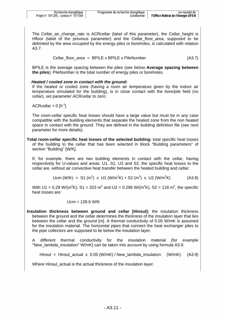
Recherche énergétique Projet n° 101’295, contrat n° 151’549
Programme de recherche énergétique Géothermie
sur mandat de l’Office fédéral de l’énergie OFEN
- A3.11 -
The Cellar_air_change_rate is ACRcellar (label of this parameter), the Cellar_height is
Hfloor (label of the previous parameter) and the Cellar_floor_area, supposed to be delimited by the area occupied by the energy piles or boreholes, is calculated with relation A3.7.
Cellar_floor_area = BPILE x BPILE x PileNumber (A3.7)
BPILE is the average spacing between the piles (see below Average spacing between
the piles); PileNumber is the total number of energy piles or boreholes. Heated / cooled zone in contact with the ground: If the heated or cooled zone (having a room air temperature given by the indoor air
temperature simulated for the building), is in close contact with the bore/pile field (no cellar), set parameter ACRcellar to zero:
ACRcellar = 0 [h-1] The room-cellar specific heat losses should have a large value but must be in any case
compatible with the building elements that separate the heated zone from the non heated space in contact with the ground. They are defined in the building definition file (see next parameter for more details).
Total room-cellar specific heat losses of the selected building: total specific heat losses
of the building to the cellar that has been selected in block “Building parameters” of section “Building” [W/K].
If, for example, there are two building elements in contact with the cellar, having
respectively for U-values and areas: U1, S1, U2 and S2, the specific heat losses to the cellar are, without air convective heat transfer between the heated building and cellar:
Ucm (W/K) = S1 (m2) x U1 (W/m2K) + S2 (m2) x U2 (W/m2K) (A3.8)
With U1 = 0.29 W/(m2K), S1 = 323 m2 and U2 = 0.296 W/(m2K), S2 = 118 m2, the specific
heat losses are: Ucm = 128.6 W/K Insulation thickness between ground and cellar [Hinsul]: the insulation thickness
between the ground and the cellar determines the thickness of the insulation layer that lies between the cellar and the ground [m]. A thermal conductivity of 0.05 W/mK is assumed for the insulation material. The horizontal pipes that connect the heat exchanger piles to the pipe collectors are supposed to lie below the insulation layer.
A different thermal conductivity for the insulation material (for example
"New_lambda_insulation" W/mK) can be taken into account by using formula A3.9.
Hinsul = Hinsul_actual x 0.05 (W/mK) / New_lambda_insulation (W/mK) (A3.9) Where Hinsul_actual is the actual thickness of the insulation layer.
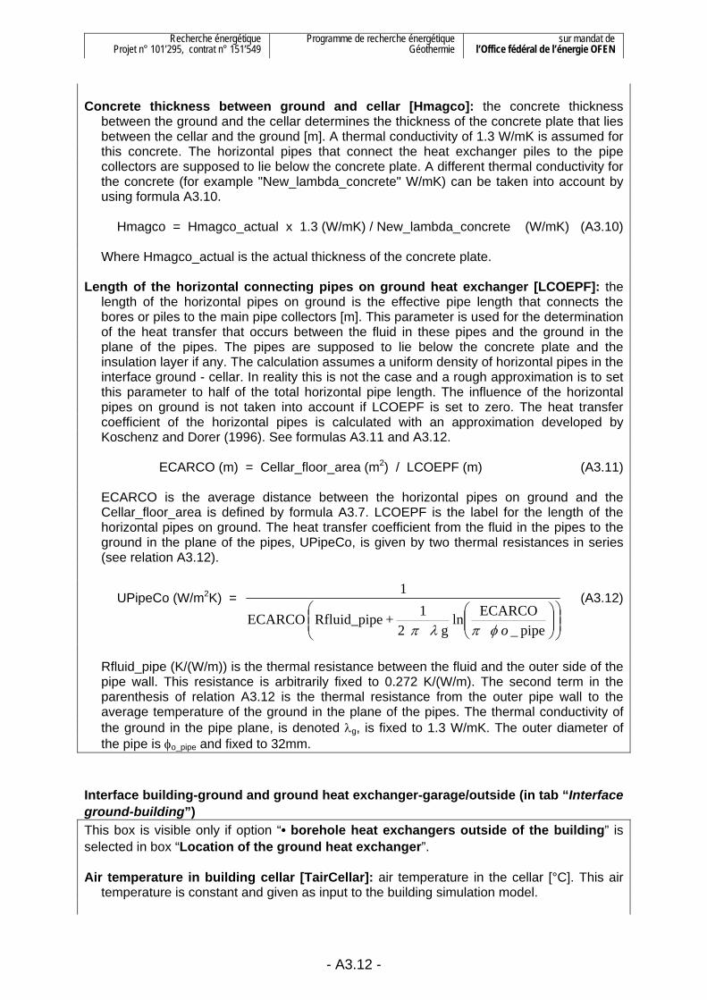
Recherche énergétique Projet n° 101’295, contrat n° 151’549
Programme de recherche énergétique Géothermie
sur mandat de l’Office fédéral de l’énergie OFEN
- A3.12 -
Concrete thickness between ground and cellar [Hmagco]: the concrete thickness
between the ground and the cellar determines the thickness of the concrete plate that lies between the cellar and the ground [m]. A thermal conductivity of 1.3 W/mK is assumed for this concrete. The horizontal pipes that connect the heat exchanger piles to the pipe collectors are supposed to lie below the concrete plate. A different thermal conductivity for the concrete (for example "New_lambda_concrete" W/mK) can be taken into account by using formula A3.10.
Hmagco = Hmagco_actual x 1.3 (W/mK) / New_lambda_concrete (W/mK) (A3.10)
Where Hmagco_actual is the actual thickness of the concrete plate. Length of the horizontal connecting pipes on ground heat exchanger [LCOEPF]: the
length of the horizontal pipes on ground is the effective pipe length that connects the bores or piles to the main pipe collectors [m]. This parameter is used for the determination of the heat transfer that occurs between the fluid in these pipes and the ground in the plane of the pipes. The pipes are supposed to lie below the concrete plate and the insulation layer if any. The calculation assumes a uniform density of horizontal pipes in the interface ground - cellar. In reality this is not the case and a rough approximation is to set this parameter to half of the total horizontal pipe length. The influence of the horizontal pipes on ground is not taken into account if LCOEPF is set to zero. The heat transfer coefficient of the horizontal pipes is calculated with an approximation developed by Koschenz and Dorer (1996). See formulas A3.11 and A3.12.
ECARCO (m) = Cellar_floor_area (m2) / LCOEPF (m) (A3.11)
ECARCO is the average distance between the horizontal pipes on ground and the
Cellar_floor_area is defined by formula A3.7. LCOEPF is the label for the length of the horizontal pipes on ground. The heat transfer coefficient from the fluid in the pipes to the ground in the plane of the pipes, UPipeCo, is given by two thermal resistances in series (see relation A3.12).
UPipeCo (W/m2K) =
⎟⎟⎠
⎞⎜⎜⎝
⎛⎟⎟⎠
⎞⎜⎜⎝
⎛pipe_
ECARCOln g 2
1 + eRfluid_pip ECARCO
1
oφπλπ
(A3.12)
Rfluid_pipe (K/(W/m)) is the thermal resistance between the fluid and the outer side of the
pipe wall. This resistance is arbitrarily fixed to 0.272 K/(W/m). The second term in the parenthesis of relation A3.12 is the thermal resistance from the outer pipe wall to the average temperature of the ground in the plane of the pipes. The thermal conductivity of the ground in the pipe plane, is denoted λg, is fixed to 1.3 W/mK. The outer diameter of the pipe is φo_pipe and fixed to 32mm.
Interface building-ground and ground heat exchanger-garage/outside (in tab “Interface ground-building”) This box is visible only if option “• borehole heat exchangers outside of the building” is selected in box “Location of the ground heat exchanger”. Air temperature in building cellar [TairCellar]: air temperature in the cellar [°C]. This air
temperature is constant and given as input to the building simulation model.

Recherche énergétique Projet n° 101’295, contrat n° 151’549
Programme de recherche énergétique Géothermie
sur mandat de l’Office fédéral de l’énergie OFEN
- A3.13 -
Constant air temperature component of garage [TconstGarage]: constant temperature
component assigned to the garage that lies over the borehole heat exchangers [°C]. The air temperature in the garage will result from the heat transfer from this constant temperature and the corresponding heat transfer coefficient UCelBu (see parameter below), heat transfer with the outside air, calculated with a constant air change rate ACRcellar, and heat transfer with the ground (top side of the ground volume enclosed by the ground heat exchanger).
If no garage is present on top of the ground heat exchanger, UCelBu can be fixed to zero
and ACRcellar to an arbitrary large value (see parameter ACRcellar below), so that the garage temperature is equal to the outside air temperature.
Height of the garage above the ground heat exchanger [Hfloor]: height of the garage
that lies above the ground heat exchanger [m]. This parameter is used to estimated the air volume of the garage for air change losses. The volume is calculated with the cellar floor area (see equation A3.7).
Air change rate in garage [ACRcellar]: this air change rate determines heat losses or heat
gains in the garage with the outdoor air [h-1]. For the sake of simplicity, the losses from the garage to the exterior (outdoor air) are only computed by ventilation losses. The specific heat losses from the garage to the exterior (Uce) are calculated using formula A3.5 and A3.6.
No garage above the ground heat exchanger: If there is no garage above the ground heat exchanger, the air temperature of the
“missing” garage should be equal to that of the outside air. This is possible by setting the parameters ACRcellar and UCelBU (next parameter) to the following values :
ACRcellar = 1025 [h-1] (and the parameter Hfloor has to be greater than 0) UCelBu = 0 [W/m2K] Heat transfer coefficient with constant air temperature component of garage [UCelBu]:
heat transfer coefficient between the constant temperature component of the garage and its resulting air temperature. The heat transfer is calculated with the specific losses coefficient Ucm. This latter is obtained with formula A3.13.
Ucm (W/K) = Cellar_floor_area (m2) x UCelBu (W/m2K) (A3.13)
See formula A3.7 for the calculation of Cellar_floor_area. No garage above the ground heat exchanger: If there is no garage above the ground heat exchanger, the air temperature of the
“missing” garage should be equal to that of the outside air. This is possible by setting the parameters ACRcellar (previous parameter) and UCelBU to the following values :
ACRcellar = 1025 [h-1] (and the parameter Hfloor has to be greater than 0) UCelBu = 0 [W/m2K]

Recherche énergétique Projet n° 101’295, contrat n° 151’549
Programme de recherche énergétique Géothermie
sur mandat de l’Office fédéral de l’énergie OFEN
- A3.14 -
Insulation thickness between ground and garage [Hinsul]: the insulation thickness
between the ground and the garage determines the thickness of the insulation layer that lies between the cellar and the ground. A thermal conductivity of 0.05 W/mK is assumed for the insulation material. The horizontal pipes that connect the bores or piles to the main pipe collectors are supposed to lie below the insulation layer. A different thermal conductivity for the insulation material (for example "New_lambda_insulation" W/mK) can be taken into account by using formula A3.9.
Concrete thickness between ground and garage [Hmagco]: the concrete thickness
between ground and garage determines the thickness of the concrete plate that lies between the ground and garage. A thermal conductivity of 1.3 W/mK is assumed for concrete. The horizontal pipes that connect the borehole heat exchangers to the main pipe collectors are supposed to lie below the concrete plate. A different thermal conductivity for concrete (for example "New_lambda_concrete" W/mK) can be taken into account by using formula A3.10.
Length of the horizontal pipes on ground [LCOEPF]: the length of the horizontal pipes on
ground is the effective pipe length that connects the borehole heat exchangers to the main pipe collectors. This parameter is used for the determination of the heat transfer that occurs between the fluid in these pipes and the ground in the plane of the pipes. The pipes are supposed to lie below the concrete plate and the insulation layer if any. The calculation assumes a uniform density of horizontal pipes in the interface ground - garage. In reality this is not the case and a rough approximation is to set this parameter to half of the total horizontal pipe length. The influence of the horizontal pipes on ground is not taken into account if LCOEPF is set to zero. The heat transfer coefficient of the horizontal pipes is calculated with formulas A3.11 and A3.12.
The Ground heat exchanger tab: Energy piles or borehole heat exchangers (in tab “Ground heat exchanger”) Up to 6 different pile/bore types can be specified. A pile/bore type is defined by its diameter, thermal resistance and average active pile/bore length. Average values are calculated from these quantities, as only one pile/bore type is simulated. Diameter of pile/borehole type i (i = 1 [dp1], 2, 3, 4, 5 or 6). This parameter determines the
diameter of pile/bore type i [m]. The average pile/bore diameter is calculated so that the total volume of piles/bores is preserved (see relation A3.14). It is written in the output parameter file with the extension ".PAR" (parameter label: AvePilDiam).
AvePilDiam = ( )
21
6
1
6
1
2
N H
N H /2dp 2
⎟⎟⎟⎟
⎠
⎞
⎜⎜⎜⎜
⎝
⎛
∑
∑
=
=
i
i
ii
iii (A3.14)
dpi is the pile/bore diameter of type i, Hi the pile/bore active length and Ni the pile/bore
number (see below).

Recherche énergétique Projet n° 101’295, contrat n° 151’549
Programme de recherche énergétique Géothermie
sur mandat de l’Office fédéral de l’énergie OFEN
- A3.15 -
Number of piles/boreholes for type i (i = 1 [N1], 2, 3, 4, 5 or 6). This parameter determines
the number of piles/bores of type i [-]. The total number of energy piles or boreholes is the sum of each pile/bore type number (see A3.15) and is written in the output parameter file with the extension ".PAR" (parameter label: PileNumber).
PileNumber = ∑=
6
1
Ni
i (A3.15)
Average active length of piles/boreholes type i (i = 1 [H1], 2, 3, 4, 5 or 6). This parameter
determines the average active pile length of pile type i [m]. The active length of a pile is defined by the pile length for which a radial heat transfer with the ground may occur. In other terms, it is the length of the pile that is equipped with pipes. The pile active length is smaller than the total pile length. An average active pile length is calculated for ALL the heat exchanger piles (see formula A3.16). It defines the vertical extension of the ground volume that contains the simulated piles. It is written in the output parameter file with the extension ".PAR" (parameter label: AvePLength).
AvePLength =
∑
∑
=
=6
1
6
1
N
H N
i
i
i
ii (A3.16)
Thermal resistance Rb of pile/borehole type i (i = 1 [Rb1], 2, 3, 4, 5 or 6). This parameter
determines the thermal resistance of pile/bore type i [K/(W/m)]. The thermal resistance of a pile/borehole determines the temperature difference between the fluid and the ground in the immediate vicinity of the pile/borehole under a given heat transfer rate. For example, a thermal resistance value of 0.1 K/(W/m) will induce a temperature difference of 5 K between the fluid temperature and the ground temperature at the pile/bore border, when a heat transfer rate of 50 W/m takes place in steady flux conditions in the pile/bore. For more information on pile thermal resistances, see Fromentin et al., 1997. For borehole thermal resistances, the use of the programme EED (Earth Energy Designer) is recommended (Hellström and Sanner, 1994). In EED, a tool for the calculation of borehole thermal resistances with single, double, triple U-pipe or coaxial pipes is integrated. Other pipe configurations in a borehole or a pile can be treated with the programme MPC (Bennet et al., 1987). Some thermal resistance values are given below.
Energy pile thermal resistances: 0.15 K/(W/m) hollow prefabricated pile with a double U-pipe, pile diameter: 30
to 50 cm; 0.10 - 0.11 K/(W/m) pre-cast or cast in place pile, double U-pipe fixed on the
metallic reinforcement. Pile diameter: 30 to 150 cm; 0.07 - 0.08 K/(W/m) pre-cast or cast in place pile, triple U-pipe fixed on the metallic
reinforcement. Pile diameter: 30 to 150 cm; 0.06 K/(W/m) pre-cast or cast in place pile, quadruple U-pipe fixed on the
metallic reinforcement. Pile diameter: 30 to 150 cm; Borehole thermal resistances: A typical value of 0.1 K/(W/m) is representative for a double U-pipe in a borehole of
diameter 10 to 15 cm.

Recherche énergétique Projet n° 101’295, contrat n° 151’549
Programme de recherche énergétique Géothermie
sur mandat de l’Office fédéral de l’énergie OFEN
- A3.16 -
An average pile/bore thermal resistance is calculated for ALL the energy piles/boreholes with the help of formula A3.17. The average pile/bore thermal resistance is calculated relatively to the average pile diameter (AvePilDiam). It is written in the output parameter file with the extension ".PAR" (parameter label: AveRbPile).
dpAvePilDiamln
avegr 21 + Rb
1N H = AveRbPile
1 N H6
1
6
1∑∑
==
⎪⎪
⎭
⎪⎪
⎬
⎫
⎪⎪
⎩
⎪⎪
⎨
⎧
⎟⎟⎠
⎞⎜⎜⎝
⎛⎟⎟⎠
⎞⎜⎜⎝
⎛ii
ii
iiii
λπ
(A3.17)
λavegr is the average ground thermal conductivity. This value takes into account the
thermal conductivity of each ground layer which is crossed by the average active pile/bore length (AvePLength). It also takes into account the influence of a regional ground water flow by using the correction factor applied on the thermal conductivity (see section 7.2 of PILESIM2 user manual).
Internal thermal resistance Ra of pile/borehole type i (i = 1 [Ra1], 2, 3, 4, 5 or 6). This
parameter determines the internal thermal resistance of the piles/boreholes [K/(W/m)]. The internal thermal resistance of a pile/bore determines the internal heat transfers within the pile/bore.
A typical value is comprised between 0.1 - 0.4 K/(W/m) for a double U-pipe in a borehole
heat exchanger. Average spacing between the piles/boreholes [BPILE]: this parameter specifies the
effective average spacing of ALL the piles/boreholes in the TWO spatial directions of the ground area that contains the piles/boreholes [m]. This parameter determines the ground volume (GrndVolume) that is ascribed to the piles/boreholes with relation A3.18.
GrndVolume = (BPILE)2 x PileNumber x AvePLength (A3.18)
See equations A3.15 and A3.16 for the total number of energy piles/boreholes
(PileNumber) and the average active pile/bore length (AvePLength). The average spacing between the piles/bores is called BPILE. The ground volume used for the simulation is written in the output parameter file with the extension ".PAR" (parameter label: GrndVolume).
The best pile/bore arrangement for increased thermal performances is obtained with a
regular spacing between the piles/boreholes. If the shape of the area occupied by the piles/bores is close to a square, then the average spacing is easy to calculate.
A method to establish this parameter is to draw a line around the ground area that is occupied by the piles/boreholes. A "half average spacing" is maintained between the line and the piles/bores in the periphery. The area drawn by this line is then divided by the total number of energy piles/boreholes, and the average spacing is obtained by taking the square root of this number.
If the energy piles/boreholes are not uniformly placed within this area, it will result in a
smaller average spacing. However, the effective average spacing remains greater than the smallest spacing between two energy piles/boreholes.

Recherche énergétique Projet n° 101’295, contrat n° 151’549
Programme de recherche énergétique Géothermie
sur mandat de l’Office fédéral de l’énergie OFEN
- A3.17 -
If the shape of the area that contains the piles/bores is close to a rectangle which is
characterised by a large difference between its width and its length, then the average spacing will tend to be greater. As an example, about 200 heat exchanger piles uniformly placed in a rectangular shape of 500m x 30m were simulated. The calibration described below resulted in an increase of the average spacing from 9.3 to 10.1 m, thus less than 10%.
A more accurate method is to calibrate the model used in COOLSIM with a model that takes into account the exact position of the piles/bores. It can be done with TRNSBM, the Superposition Borehole Model.
Number of piles/boreholes coupled in series [NSERIE]. This parameter determines the
number of piles/bores that are connected in series [-]. As the simulation model simulates a cylinder, a radial interconnection of the piles/bores is taken into account.
Pipe configuration in pile/borehole. The two possible pipe configuration in the pile/bore
are: U-pipe configuration: the pipe installation in the pile/bore is formed by one or more U-
pipes placed close to the circumference of the pile/borehole. Coaxial pipe installation: the pipe installation in the pile/bore is formed by a coaxial pipe. Pipe number in a cross section of a pile/borehole: average number of pipes in a pile/bore
cross section [-]. This number is used to estimate the total volume of fluid that is contained in the energy piles/boreholes. This parameter is only used to take into account the heat capacitive effects of the heat carrier fluid in the piles/bores. The total volume of heat carrier fluid contained in the piles is calculated with relation A3.19.
Fluid_volume = NTUB x π x (Inner_pipe_radius)2 x PileNumber x AvePLength (A3.19)
NTUB is the pipe number in a pile/bore cross section; Inner_pipe_radius is defined with
the next input parameter (pipe number in a cross section of a pile); PileNumber and AvePLength are respectively the total number and the average active length of the energy piles/boreholes. If Fluid_volume, the volume of heat carrier fluid in the piles/bores, is known, then relation A3.19 can be used to calculate the average number of pipes in a pile/bore cross section.
Inner diameter of one pipe: this parameter represents the average inner diameter of the
pipes in the energy piles/bores [mm]. It is only used to estimate the total volume of fluid that is contained in the energy piles/boreholes with relation A3.19. The total volume of fluid is only used to take into account the heat capacitive effects of the heat carrier fluid in the piles/bores.
Fraction of pile/borehole concrete/filling thermal capacity: this parameter defines the
fraction of the pile concrete/bore filling material in the active zone of a pile/bore which contributes to heat capacitive effects [%]. The active zone of a pile/bore is the part that is equipped with plastic pipes for the heat transfer with the ground, i.e. the heat exchanger. A typical value of 50% was found to satisfactorily match measured data of a pile system (pile diameter of 30 to 40 cm). A large value may produce an error which aborts the programme when run. An error message is written in the listing file (COOLSIM.LST). Do not forget to read a possible error message near the end of this file if you can not run your case.

Recherche énergétique Projet n° 101’295, contrat n° 151’549
Programme de recherche énergétique Géothermie
sur mandat de l’Office fédéral de l’énergie OFEN
- A3.18 -
If borehole heat exchangers are simulated, the heat capacitive effects are small and a
fraction of 0 can be set. The heat capacitive effects of the pile concrete are calculated with an effective pile
diameter and an effective pile thermal resistance (see equation A3.20 and A3.21). They are written in the output parameter file with the extension ".PAR" (the parameter labels are respectively: EffPilDiam and EffRbPil).
EffPilDiam = AvePilDiam ( )21
eGrndCap)(Cconcr/Av FrCapa - 1 (A3.20) AvePilDiam is the average pile diameter (see equation A3.14); FrCapa is the fraction of
pile thermal capacity taken into account; Cconcr is the volumetric heat capacity of the pile concrete (Cconcr is set to 2’592 kJ/m3K); AveGrndCap is the average volumetric heat capacity of the ground in the zone crossed by the average active pile length.
EffRbPile = AveRbPile ⎟⎠⎞
⎜⎝⎛−
EffPilDiamAvePilDiamln
avegr 21
λπ (A3.21)
AveRbPile is the average pile thermal resistance and λavegr is the average ground thermal
conductivity (see equation A3.17). AvePilDiam and EffPilDiam are respectively the average pile diameter and the effective average pile diameter (see equations A3.14 and A3.20).
The Ground characteristics tab: Ground characteristics: Up to 3 different horizontal ground layers can be specified. A ground layer is defined by its thickness, the thermal conductivity and volumetric heat capacity of the ground and the Darcy velocity of the water contained in the ground layer. Initial ground temperature [TGRDIN]: this parameter specifies the initial temperature of the
ground before the construction of the building [°C]. This temperature should be set to the annual average value of the ground near the surface. A rough estimation is to use the mean annual air temperature at the surface.
Mean temperature gradient in the undisturbed ground [dTGRND]: geothermal
temperature gradient present at the project location [K/km]. Assumed to be constant, it defines the temperature increase in the ground with depth.
Thermal conductivity of ground layer i [LGi] (i = 1, 2 and 3): this parameter sets the
thermal conductivity of ground layer i [W/(mK)]. For water saturated soils that requires the use of foundation piles, a typical value of 2 W/mK can be assumed. More information on ground thermal conductivity can be found for example in Fromentin et al., 1997 or Hellström and Sanner, 1994.
Volumetric thermal capacity of layer i [CGi] (i = 1, 2 and 3): this parameter sets the
volumetric thermal capacity of ground layer i [MJ/(m3K)]. For water saturated soils that requires the use of foundation piles, typical values lie between 2 and 3 MJ/m3K. More information on ground volumetric thermal capacity can be found for example in Fromentin et al., 1997 or Hellström and Sanner, 1994.

Recherche énergétique Projet n° 101’295, contrat n° 151’549
Programme de recherche énergétique Géothermie
sur mandat de l’Office fédéral de l’énergie OFEN
- A3.19 -
Thickness of ground layer i (i = 1, 2 and 3): this parameter sets the thickness of ground
layer i [m]. The first ground layer must be larger than 0.3m, which is the layer 0, in which lie the horizontal pipes that connect the bores or piles to the heat pump. The thickness of ground layer 3, which is the lowest ground layer, is supposed to extend downward as far as necessary by the thermal calculations.
Darcy velocity of ground water in layer i [DAi] (i = 1, 2 and 3): this parameter sets the
Darcy velocity of the ground water in the ground layer i [m/day]. This parameter determines the forced convection in the ground layer i due to a horizontal regional ground water flow. A zero value means no forced convection. The Darcy velocity (in m/s) can be obtained by the product of the ground layer permeability (in m/s) times the horizontal hydraulic gradient of the regional ground water flow (in m/m). More information on ground permeability can be found for example in Fromentin et al., 1997.
NB: only a direct thermal interaction with the piles/bores is computed. In other terms, if the
ground layer i lies below the bottom of the piles/bores, the effect of a regional ground water flow will not be computed. If only the upper part of ground layer i is crossed by the energy piles/boreholes, the effect will be computed in the upper part only. The thermal influence will be then propagated upwards and downwards by pure heat conduction.
NB: the full influence of a ground water flow is only calculated if the following two
parameters switches are “ON”. Simulate forced convection on global process: this parameter determines if the global
effect of the forced convection is taken into account (see below). YES: global effect of forced convection taken into account; NO: global effect of forced convection not taken into account. Simulate forced convection on local process: this parameter determines if the local effect
of the forced convection is taken into account (see below). YES: local effect of forced convection taken into account; NO: local effect of forced convection not taken into account. The effect of forced convection is treated as the superposition of two effects: the global process: a heat balance of the heat transfer by forced convection is performed on the boundary of
the ground volume that is ascribed to the energy piles/boreholes. The heat quantity transferred by forced convection to or from the ground volume is treated as a global temperature change of the ground temperature in the volume. The global process takes into account long term effects, which, in particular, determine the magnitude of a natural thermal recharge of the ground by a regional ground water flow.
the local process: for the case of pure heat conduction, a temperature gradient takes place around the
energy piles/boreholes when they are used to transfer heat with the ground. As a result, the heat transfer is limited by the presence of a local temperature difference between the piles/bores and the mean ground temperature. If ground water flows across the piles/bores, the temperature field will be shifted. For a sufficiently large flow, the local temperature difference will be decreased and the heat transfer between the piles/bores and the ground improved. The local process takes into account the improvement of this heat transfer.

Recherche énergétique Projet n° 101’295, contrat n° 151’549
Programme de recherche énergétique Géothermie
sur mandat de l’Office fédéral de l’énergie OFEN
- A3.20 -
A3.1.6. How to Run COOLSIM2 Once the data are defined as desired, it is recommended to save the data before a simulation is started. The input data are saved in the file COOLSIM.TRD. It is done in the File / Save menu of the TRNSED programme. A simulation is started in the menu TRNSYS / Calculate. A series of simulations can also be defined and then simulated. The user is advised to read the help provided with the TRNSED programme. It is found in the menu Help / TRNSED Help, and then look for the topic Parametrics Menu. When a series of simulations is performed, a New Table is created in the menu Parametrics. An existing table can be opened in the menu Windows and selection Table. All the parameters that can be varied are listed. The user selects the desired parameter to be varied and defines the ranges of variations. The units of the parameters must correspond to the primary units. In table A3.1 are listed all the parameter that can be varied, together with their primary units and the conversion factor from secondary units. Parameter Short description Primary unit = sec. unit x factor
ACRCELLAR Air change rate in cellar or garage h-1 = h-1
ACRMECHANIC Nominal air change rate of mechanical system ventilation h-1 = h-1
ACRNIGHT Air change rate for night cooling h-1 = h-1
AIRHXEFFICIENCY Efficiency of the mechanical system heat recovery units - = -
AZIMSUD Azimuth of south façade ° = °
BPILE Average spacing between the piles or boreholes m = m
CG1 Volumetric heat capacity of ground layer 1 kJ/(m3K) = MJ/(m3K) x 1000
CG2 Volumetric heat capacity of ground layer 2 kJ/(m3K) = MJ/(m3K) x 1000
CG3 Volumetric heat capacity of ground layer 3 kJ/(m3K) = MJ/(m3K) x 1000
COPo Design performance coefficient - = -
DA1 Darcy velocity of ground water in layer 1
m/s = m/day x (1/86’400)
DA2 Darcy velocity of ground water in layer 2
m/s = m/day x (1/86’400)
DA3 Darcy velocity of ground water in layer 3
m/s = m/day x (1/86’400)
Table A3.1 List of the parameters that can be varied in a multiple simulation

Recherche énergétique Projet n° 101’295, contrat n° 151’549
Programme de recherche énergétique Géothermie
sur mandat de l’Office fédéral de l’énergie OFEN
- A3.21 -
Parameter Short description Primary
unit = sec. unit x factor
DP1 Diameter of pile or borehole type 1 m = m
DTGRND Mean temperature gradient in the undisturbed ground K/m = K/km x (1/1’000)
ESHADESUMMER External shading device efficiency in Summer - = -
ESHADEWINTER External shading device efficiency in Winter - = -
FLOWSPECTABS Fluid flow rate per square meter of heated or cooled concrete plate (TABS)
(kg/h)/m2 = (kg/h)/m2
H1 Average active length of pile or borehole type 1 m = m
HFLOOR Height of garage or cellar between rooms and ground m = m
HG11 Thickness of ground layer 1 m = m
HG2 Thickness of ground layer 2 m = m
HG3 Thickness of ground layer 3 m = m
HINSUL Insulation thickness between ground and cellar m = m
HMAGCO Concrete thickness between ground and cellar or garage m = m
HXUAGEO Design heat transfer coefficient of geocooling counterflow heat exchanger
kJ/(hK) = kW/K x 3’600
ISHADESUMMER Internal shading device efficiency in Summer - = -
ISHADEWINTER Internal shading device efficiency in Winter - = -
IVLIMITSUMMER Vertical global solar radiation limit to use solar protections in Summer W/m2 = W/m2
IVLIMITWINTER Vertical global solar radiation limit to use solar protections in Winter W/m2 = W/m2
LCOEPF Length of the horizontal pipes on top of energy piles or borehole heat exchangers
m = m
LG1 Thermal conductivity of first ground layer kJ/(h m K) = W/(mK) x 3.6
LG2 Thermal conductivity of second ground layer kJ/(h m K) = W/(mK) x 3.6
LG3 Thermal conductivity of third ground layer kJ/(h m K) = W/(mK) x 3.6
Table A3.1 List of the parameters that can be varied in a multiple simulation (continued)

Recherche énergétique Projet n° 101’295, contrat n° 151’549
Programme de recherche énergétique Géothermie
sur mandat de l’Office fédéral de l’énergie OFEN
- A3.22 -
Parameter Short description Primary unit = sec. unit x factor
N1 Number of piles or boreholes for type 1 - = -
NSERIE Number of piles or boreholes coupled in series - = -
PHEATDESIGN Design thermal power of the heat pump kJ/h = kW x 3’600
RA1 Internal thermal resistance Ra of pile or borehole type 1 K/(kJ/hm) = K/(W/m) x (1/3.6)
RB1 Thermal resistance Rb of pile or borehole type 1 K/(kJ/hm) = K/(W/m) x (1/3.6)
RTABS Thermal resistance fluid-concrete in activated concrete plates (TABS)
K/(W/m2) = K/(W/m2)
SCALEGAININT Scaling factor for internal heat gains - = -
TAIRCELLAR 1) Air temperature in building cellar °C = °C
TCONSTGARAGE 1) Constant air temperature component of garage °C = °C
TCOOLDESIGN Design forward fluid temperature for cooling °C = °C
TFMIN Minimum allowed fluid temperature in the pile or borehole flow circuit
°C = °C
TGRDIN Mean undisturbed ground temperature at the surface °C = °C
TLIMITSUMMER Daily temperature limit to allow cooling operation °C = °C
TLIMITVENTHX Daily temperature limit to control heat recovery operation °C = °C
TSETCOOLINGHIGH Set point temperature to switch on cooling °C = °C
TSETCOOLINGLOW Set point temperature to switch off cooling °C = °C
TSETHEATINGHIGH Set point temperature to switch off heating °C = °C
TSETHEATINGLOW Set point temperature to switch on heating °C = °C
UCELBU 1) Heat transfer coefficient with constant air temperature component of garage
kJ/(h m2 K) = W/(m2K) x 3.6
1) Only for case “borehole heat exchangers” outside of the building Table A3.1 List of the parameters that can be varied in a multiple simulation (continued) If a parametric study is performed with the borehole parameters (RB1, RA1, N1, H1), it is best to define only one type of BHE.

Recherche énergétique Projet n° 101’295, contrat n° 151’549
Programme de recherche énergétique Géothermie
sur mandat de l’Office fédéral de l’énergie OFEN
- A3.23 -
A multiple simulation is started once a parameter table has been created, using the command Run Table in the TRNSYS menu. A3.1.7. Output Data from COOLSIM2 The output data from COOLSIM2 are written in 15 different files. Three files contain the input information given to COOLSIM2 and possible error messages, and 12 files contains the calculated quantities by COOLSIM2. Assuming that the file containing the input data is called COOLSIM.TRD, the following files are written: • COOLSIM.LST (listing file) • DST.DAT (input data related to TRNVDSTP) • COOLSIM.PAR (calculated parameters) • COOLSIM.EXT (output data, maximum and minimum thermal powers and
temperatures) • COOLSIM.OU1 (output data, mean temperatures, integrated quantities) • COOLSIM.OU2 (output data, mean temperatures, integrated quantities) • COOLSIM.OU3 (output data, mean temperatures, integrated quantities) • COOLSIM.OU4 (output data, mean temperatures, integrated quantities) • COOLSIM.OU5 (output data, mean temperatures, integrated quantities) • COOLSIM.OU6 (output data, mean temperatures, integrated quantities) • COOLSIM.OU7 (output data, mean temperatures, integrated quantities) • COOLSIM.OU8 (output data, mean temperatures, integrated quantities) • COOLSIM.OU9 (output data, mean temperatures, integrated quantities) • COOLSIM.PL1 (output data, evolution of selected variables) • COOLSIM.PL2 (output data, evolution of selected variables) When a simulation is completed, the file COOLSIM.LST can be viewed in the Windows menu of the TRNSED programme, and the files COOLSIM.OUi in the Windows / Other files menu. A plot can be made with the file COOLSIM.PLi and viewed in the Plot menu. The Listing File COOLSIM.LST This is the listing file written by TRNSYS. All the information contained in COOLSIM.TRD is written in the listing file, together with some information related to the simulation itself (simulation duration, total number of calls for each component, warning message if any, etc.). It should be noted that if an error makes a simulation to abort, the corresponding error message is written at the end of the listing file. It is recommended to read this file every time a simulation is terminated with an error. The File DST.DAT This file is written by the TRNVDSTP component which simulates the borehole heat exchanger field. It contains all the parameters used by this component, together with information on the fields used for the simulation of the heat transport in the ground.

Recherche énergétique Projet n° 101’295, contrat n° 151’549
Programme de recherche énergétique Géothermie
sur mandat de l’Office fédéral de l’énergie OFEN
- A3.24 -
The Output File COOLSIM.PAR This file contains some of the mean parameter values which are calculated and used for the simulation. They are: PileNumber [-] : total number of energy piles/boreholes (cf. equation A3.15). AvePLength [m] : average active pile length of the energy piles/boreholes (cf. equation
A3.16). GrndVolume [m3]: ground volume ascribed to the energy piles/boreholes (cf. equation
A3.18). AvePilDiam [m] : average pile/borehole diameter (cf. equation A3.14). EffPilDiam [m] : effective pile/borehole diameter for heat capacitive effects (cf. equation
A3.20). AveRbPile [K/(W/m)]: average pile/borehole thermal resistance (cf. equation A3.17). EffRbPile [K/(W/m)]: effective pile/borehole thermal resistance for heat capacitive
effects (cf. equation A3.21). FlowRate [kg/h]: total flow rate through the pile/bore circuit when heating (i.e. when the
heat pump is on. See the description of parameter “design inlet-outlet temperature difference in evaporator (PAC)”, in section A3.5.3).
AveEfGrndL [W/mK]: effective mean thermal conductivity in the ground volume GrndVolume (the effective value includes the effect of forced convection on the local problem, see comment for λavegr in equation A3.17).
AveGrndCap [kJ/m3K]: mean volumetric heat capacity in the ground volume GrndVolume (see comment for equation A3.20).
The Output File COOLSIM.EXT Maximum or minimum values of some selected quantities are calculated on a regular time interval (month or year). MaxHeatDem [kW]: maximum hourly heat demand of the system during the month or the
year. MaxExtPile [kW]: maximum hourly heat power extracted from the piles/bores during the
month or the year. MaxColdDem [kW]: maximum hourly cold demand of the system during the month or the
year. MaxInjPile [kW]: maximum hourly heat power injected through the piles/bores during
the month or the year. TinPileMin [degree C]: minimum inlet fluid temperature in the piles/bores during the
month or the year. TinPileMax [degree C]: maximum inlet fluid temperature in the piles/bores during the
month or the year.
Recherche énergétique Projet n° 101’295, contrat n° 151’549
Programme de recherche énergétique Géothermie
sur mandat de l’Office fédéral de l’énergie OFEN
- A3.25 -
The Output File COOLSIM.OU1 Integrated or average quantities of various quantities are calculated on a regular time interval (month or year). They are produced with the help of 9 simulation summary type components and written in 9 different files. The results of the first simulation summary are written in the file COOLSIM.OU1. The labels of each calculated quantity are for the first the simulation summary: TairExt [°C]: mean outdoor air temperature. Tsky [°C]: mean sky temperature. HHor [kWh/m2]: mean global solar radiation on horizontal plane. HEast [kWh/m2]: mean global solar radiation in east vertical façade. HWest [kWh/m2]: mean global solar radiation in west vertical façade. HSouth [kWh/m2]: mean global solar radiation in south vertical façade. HNorth [kWh/m2]: mean global solar radiation in north vertical façade. The Output File COOLSIM.OU2 SQheat [MJ/m2]: sum of sensible heating demand for heated zones (zone 1 and 2). SQcool [MJ/m2]: sum of sensible cooling demand for cooled zones (zone 1 and 2). SQUA [MJ/m2]: sum of static transmission losses (UA*dT) of heated/cooled zones
(zone 1 and 2). SQVENT [MJ/m2]: sum of sensible ventilation gains of heated/cooled zones (zone 1
and 2). SQINF [MJ/m2]: sum of sensible infiltration gains of heated/cooled zones (zone 1
and 2). SQGCONV [MJ/m2]: sum of internal convective gains of heated/cooled zones (zone 1
and 2). SQGRAD [MJ/m2]: sum of internal radiative gains of heated/cooled zones (zone 1 and
2). SQSOLT [MJ/m2]: sum of shortwave solar radiation transmitted through windows of
heated/cooled zones (zone 1 and 2). SQSEC [MJ/m2]: sum of secondary heat flux of all windows of heated/cooled zones
(zone 1 and 2). The Output File COOLSIM.OU3 uso_AULA_INV [h]: cumulated occupation time of the building during the Winter period,
defined when cooling is not allowed (see parameter TlimitSummer in section A3.5.2).
ore_meno_20_AULA [h]: cumulated time when the operative indoor air temperature of the “aula” zone is below 20°C during the building occupation time and Winter period.

Recherche énergétique Projet n° 101’295, contrat n° 151’549
Programme de recherche énergétique Géothermie
sur mandat de l’Office fédéral de l’énergie OFEN
- A3.26 -
rat_ore_meno_20_AULA [-]: ratio of time when the operative indoor air temperature of the “aula” zone is below 20°C during Winter period and building occupation time. It is the ratio ore_meno_20_AULA/uso_AULA_INV.
gr_ore_meno_20_AULA [Kh]: cumulated degree-hours when the operative indoor air temperature of the “aula” zone is below 20°C during Winter period and building occupation time.
uso_AULA_EST [h]: cumulated occupation time of the building during the Summer period, defined when cooling is allowed (see parameter TlimitSummer in section A3.5.2).
ore_piu_26_AULA [h]: cumulated time when the operative indoor air temperature of the “aula” zone is over 26°C during the building occupation time and Summer period.
rat_ore_piu_26_AULA [-]: ratio of time when the operative indoor air temperature of the “aula” zone is over 26°C during Summer period and building occupation time. It is the ratio ore_piu_26_AULA/uso_AULA_EST.
gr_ore_piu_26_AULA [Kh]: cumulated degree-hours when the operative indoor air temperature of the “aula” zone is over 26°C during Summer period and building occupation time.
OpTempAULA [°C]: mean operative indoor air temperature of the “aula” zone. ore_piu_26_5_AULA [°C]: cumulated time when the indoor air temperature of the “aula”
zone is over 26.5°C during the building occupation time. The Output File COOLSIM.OU4 uso_AULA_EST [h]: cumulated occupation time of the building during the summer period,
defined when cooling is allowed (see parameter TlimitSommer in section A3.5.2).
ore_piu_cat1 [h]: cumulated time when the operative indoor air temperature of the “aula” zone is over the top limit value for category 1 (according to standard DIN EN 15251) during summer period and building occupation time.
ore_piu_cat2 [h]: cumulated time when the operative indoor air temperature of the “aula” zone is over the top limit value for category 2 (according to standard DIN EN 15251) during summer period and building occupation time.
ore_piu_cat3 [h]: cumulated time when the operative indoor air temperature of the “aula” zone is over the top limit value for category 3 (according to standard DIN EN 15251) during summer period and building occupation time.
rat_ore_meno_cat1 [-]: ratio of time when the operative indoor air temperature of the “aula” zone is below the top limit value for category 1 (according to standard DIN EN 15251) during summer period and building occupation time.
rat_ore_piu_cat1 [-]: ratio of time when the operative indoor air temperature of the “aula” zone is over the top limit value for category 1 (according to standard DIN EN 15251) during summer period and building occupation time.
rat_ore_piu_cat2 [-]: ratio of time when the operative indoor air temperature of the “aula” zone is over the top limit value for category 2 (according to standard DIN EN 15251) during summer period and building occupation time.

Recherche énergétique Projet n° 101’295, contrat n° 151’549
Programme de recherche énergétique Géothermie
sur mandat de l’Office fédéral de l’énergie OFEN
- A3.27 -
rat_ore_piu_cat3 [-]: ratio of time when the operative indoor air temperature of the “aula” zone is over the top limit value for category 3 (according to standard DIN EN 15251) during summer period and building occupation time.
HoursHeat [h]: duration in hours of heating operation. It is calculated as the time integration of the heating control signal.
HoursCool [h]: duration in hours of cooling operation. It is calculated as the time integration of the cooling control signal. If no geocooling energy can be delivered due to too warm ground temperatures, the cooling requirement of the building can not be satisfied and the cooling control signal will stay on, thus leading to a longer cooling operation duration.
The Output File COOLSIM.OU5 gr_ore_piu_cat1 [Kh]: cumulated degree-hours when the operative indoor air temperature of
the “aula” zone is over the top limit value for category 1 (according to standard DIN EN 15251) during summer period and building occupation time.
gr_ore_piu_cat2 [Kh]: cumulated degree-hours when the operative indoor air temperature of the “aula” zone is over the top limit value for category 2 (according to standard DIN EN 15251) during summer period and building occupation time.
gr_ore_piu_cat3 [Kh]: cumulated degree-hours when the operative indoor air temperature of the “aula” zone is over the top limit value for category 3 (according to standard DIN EN 15251) during summer period and building occupation time.
gr_ore_meno_cat1 [Kh]: cumulated degree-hours when the operative indoor air temperature of the “aula” zone is below the low limit value for category 1 (according to standard DIN EN 15251) during summer period and building occupation time.
gr_ore_meno_cat2 [Kh]: cumulated degree-hours when the operative indoor air temperature of the “aula” zone is below the low limit value for category 2 (according to standard DIN EN 15251) during summer period and building occupation time.
gr_ore_meno_cat3 [Kh]: cumulated degree-hours when the operative indoor air temperature of the “aula” zone is below the low limit value for category 3 (according to standard DIN EN 15251) during summer period and building occupation time.
The Output File COOLSIM.OU6 This output file is the same as the one produced with PILESIM and not all the output variables are relevant and used. QHeat [kWh]: total energy demand for heating. QHeatCov [kWh]: heating energy covered by the heat pump. Auxiliary heating energy:

Recherche énergétique Projet n° 101’295, contrat n° 151’549
Programme de recherche énergétique Géothermie
sur mandat de l’Office fédéral de l’énergie OFEN
- A3.28 -
QHeatAux = QHeat – QHeatCov QCold [kWh]: total energy demand for cooling. QColdCov [kWh]: cooling energy covered by the pile/bore system (geocooling and
cooling machine). Auxiliary cooling energy: QColdAux = QCold – QColdCov QElecTot [kWh]: total electric energy used by the pile/bore system; (heat pump,
cooling machine but without circulation pumps). Electric energy used by the heat pump: QelPAC = QHeatCov/COP Electric energy used by the cooling machine: QelCoolM = QElecTot – QelPAC QHeatPil [kWh]: heating energy covered by the heat pump coupled to the
piles/boreholes. The rest, QHeatCov-QHeatPil, is covered by the heat pump coupled to the cold energy demand.
QFreeCool [kWh]: cooling energy that is provided by geocooling with the piles/boreholes. The rest, QColdCov-QFreeCool, is provided by the heat pump (extracted energy at the evaporator when there is a simultaneous demand for heating and cooling, i.e. see below QHextCold), and the cooling machine (if any). The energy extracted from the cold demand by the cooling machine is:
QCoolMach = QColdCov – QFreeCool – QHextCold COP [-]: average performance coefficient of the heat pump. It is defined as the
ratio of the delivered heating energy by the electric energy used by the heat pump:
COP = QHeatCov/QelPAC COPglobal [-]: mean performance coefficient including the cooling machine: COPglobal = (QHeatCov + QHCoolMach)/QElecTot Where QHCoolMach is the waste heat energy dissipated in the ground by
the cooling machine: QHCoolMach = QHinjGrnd – QFreeCool EffCoolM [-]: average efficiency of the cooling machine: EffCoolM = QCoolMach/QelCoolM QCoolMach = QColdCov – QFreeCool – QHextCold QelCoolM = QElecTot – QHeatCov/COP The Output File COOLSIM.OU7 This output file is the same as the one produced with PILESIM and not all the output variables are relevant and used. QHextCold [kWh]: energy extracted from the cold demand by the heat pump for heating
purposes.

Recherche énergétique Projet n° 101’295, contrat n° 151’549
Programme de recherche énergétique Géothermie
sur mandat de l’Office fédéral de l’énergie OFEN
- A3.29 -
QHextGrnd [kWh]: energy extracted from the ground by the heat pump. QHinjGrnd [kWh]: energy injected into the ground (geocooling and cooling machine).
The energy injected into the ground by the cooling machine is: QHCoolMach = QHinjGrnd – QFreeCool GrndRatio [-]: ratio energy injected in the ground over energy extracted from the
ground: GrndRation = QHinjGrnd/QHextGrnd FracHeat [-]: fraction of the total heat demand covered by the heat pump: FracHeat = QHeatCov/QHeat Qext/mPil [kWh/m]: energy extracted from the ground per energy pile/bore meter. FracCold [-]: fraction of the total cold demand covered by the pile/bores system
(pile/bores and cooling machine): FracCold = QColdCov/QCold Qinj/mPil [kWh/m]: energy injected into the ground per energy pile/bore meter. The Output File COOLSIM.OU8 This output file is the same as the one produced with PILESIM and not all the output variables are relevant and used. TmInbuild [degree C]: air temperature in the heated (or cooled) rooms. TmCellar [degree C]: air temperature in the cellar. TmSurfFlo [degree C]: surface temperature of the cellar floor. TmGrndTop [degree C]: mean temperature of the 30 cm thick ground layer that contains
the horizontal connection pipes. TmGround [degree C]: mean temperature of the ground volume that is ascribed to the
energy piles/bores. QBuiToCel [kWh]: thermal energy transferred from the heated (or cooled) rooms to the
cellar. A negative value means thermal energy transferred from the cellar to the ground.
QCelToOut [kWh]: thermal energy transferred from the cellar to outside. A negative value means thermal energy transferred from outside to the cellar.
QCelToGrd [kWh]: thermal energy transferred from the cellar to the ground. A negative value means thermal energy transferred from the ground to the cellar.
QTotExtGd [kWh]: total energy extracted from the ground by the pile/bore system. Only the hourly values of the extracted energy from the piles/bores are summed.
QHoPipExt [kWh]: energy extracted from the ground by the horizontal connection pipes. The hourly heat transfer values are summed only when heat is extracted from these pipes.
Recherche énergétique Projet n° 101’295, contrat n° 151’549
Programme de recherche énergétique Géothermie
sur mandat de l’Office fédéral de l’énergie OFEN
- A3.30 -
The Output File COOLSIM.OU9 This output file is the same as the one produced with PILESIM and not all the output variables are relevant and used. QDSTtoGrd [kWh]: thermal energy injected in the ground through the piles/bores alone
(without the horizontal connection pipes). A negative value means extracted energy.
QPIPtoGrd [kWh]: thermal energy injected in the ground through the horizontal connection pipes. A negative value means extracted energy.
QlossOut [kWh]: total heat losses from the ground volume ascribed to the energy piles/bores. A negative value is a heat gain.
QEDSTin [kWh]: variation of the internal energy of the ground in the volume ascribed to the piles/bores. A positive value means stored energy, i. e., a global increase of the ground temperatures. A negative value means a cooling of the ground temperatures.
ERRDS% [%]: error on the heat balance performed on the ground volume ascribed to the piles/bores (for calculation control).
ErrorExt% [%]: error on the energy extracted from the ground (for calculation control). ErrorInj% [%]: error on the energy injected into the ground (for calculation control). QlossTout [kWh]: heat losses through the top side of the ground volume ascribed to the
energy piles/bores. A negative value is a heat gain. QlossSout [kWh]: heat losses through the vertical sides of the ground volume ascribed
to the energy piles/bores. A negative value is a heat gain. QlossBout [kWh]: heat losses through the bottom side of the ground volume ascribed to
the energy piles/bores. A negative value is a heat gain. The Plot File COOLSIM.PL1 This file contains the time evolution of some temperatures and heat rates for the last year of the simulation period. Hourly values of these quantities are written in this file only if the input parameter “Print hourly values for last year” is set to “Yes”. Their labels are explained below. The 11 columns of the file are: Time [hour]: time in hours from the first hour of the year of the simulation start. T_AIR_EST [°C] : outdoor air temperature. T_RUGIADA [°C]: dew temperature of the outdoor air temperature. T_AIR_UFFICI [°C]: indoor bulk air temperature of the “uffici” zone. T_AIR_AULA [°C]: indoor bulk air temperature of the “aula” zone. T_OP_AULA [°C]: operative indoor air temperature of the “aula” zone. T_CEIL_AULA [°C]: surface temperature of the active concrete plate in the “aula” zone (ceiling). Uso_Edificio [-]: occupation status of the building (1 occupied; 0 non occupied). T_rm [°C]: daily running mean outdoor air temperature according to DIN EN
15251.
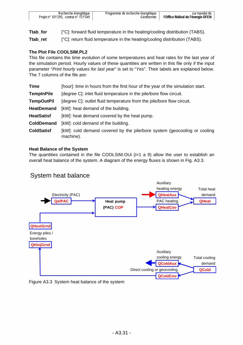
Recherche énergétique Projet n° 101’295, contrat n° 151’549
Programme de recherche énergétique Géothermie
sur mandat de l’Office fédéral de l’énergie OFEN
- A3.31 -
Ttab_for [°C]: forward fluid temperature in the heating/cooling distribution (TABS). Ttab_ret [°C]: return fluid temperature in the heating/cooling distribution (TABS). The Plot File COOLSIM.PL2 This file contains the time evolution of some temperatures and heat rates for the last year of the simulation period. Hourly values of these quantities are written in this file only if the input parameter “Print hourly values for last year” is set to “Yes”. Their labels are explained below. The 7 columns of the file are: Time [hour]: time in hours from the first hour of the year of the simulation start. TempInPile [degree C]: inlet fluid temperature in the pile/bore flow circuit. TempOutPil [degree C]: outlet fluid temperature from the pile/bore flow circuit. HeatDemand [kW]: heat demand of the building. HeatSatisf [kW]: heat demand covered by the heat pump. ColdDemand [kW]: cold demand of the building. ColdSatisf [kW]: cold demand covered by the pile/bore system (geocooling or cooling
machine). Heat Balance of the System The quantities contained in the file COOLSIM.OUi (i=1 a 9) allow the user to establish an overall heat balance of the system. A diagram of the energy fluxes is shown in Fig. A3.3.
System heat balanceAuxiliaryheating energy Total heat
Electricity (PAC) QHeatAux demandQelPAC Heat pump PAC heating QHeat
(PAC) COP QHeatCov
QHextGrnd
Energy piles /boreholesQHinjGrnd
Auxiliarycooling energy Total coolingQColdAux demand
Direct cooling or geocooling QColdQColdCov
Figure A3.3 System heat balance of the system

Recherche énergétique Projet n° 101’295, contrat n° 151’549
Programme de recherche énergétique Géothermie
sur mandat de l’Office fédéral de l’énergie OFEN
- A3.32 -
The heat quantities are calculated by the first simulation summary: QHeat [kWh]: total energy demand for heating (in COOLSIM.OU6). QHeatAux [kWh]: heating energy covered by auxiliary energy. QHeatAux = QHeat – QHeatCov QHeatCov [kWh]: heating energy covered by the heat pump (in COOLSIM.OU6). COP [-]: average performance coefficient of the heat pump (in COOLSIM.OU6). QelPAC [kWh]: electric energy used by the heat pump. QelPAC = QHeatCov/COP QHextGrnd [kWh]: energy extracted from the ground by the heat pump (in
COOLSIM.OU7). QHinjGrnd [kWh]: energy injected into the ground by geocooling and the cooling
machine (in COOLSIM.OU7). QColdAux [kWh]: cooling energy covered by auxiliary energy. QColdAux = QCold – QColdCov QColdCov [kWh]: cooling energy covered by the pile/bore system (geocooling and
cooling machine); (in COOLSIM.OU6). QCold [kWh]: total energy demand for cooling (in COOLSIM.OU6).
A3.1.8. Output Results with COOLSIM2 An excel file has been created with the name COOLSIM.XLS in order to produce graphical output results from the output files created by COOLSIM2. It contains macros that automatically open the output files, copy the content into the COOLSIM.XLS file and close them. The global system heat balance is produced together with various design quantities and files for both the building and the geothermal system. The various output results that are produced are shown in figure A3.4 to A3.11.
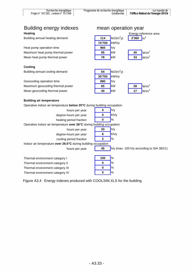
Recherche énergétique Projet n° 101’295, contrat n° 151’549
Programme de recherche énergétique Géothermie
sur mandat de l’Office fédéral de l’énergie OFEN
- A3.33 -
Building energy indexes mean operation yearHeating Energy reference areaBuilding annual heating demand 114 MJ/(m2y) 2'360 m2
74'700 kWh/yHeat pump operation time 960 h/yMaximum heat pump thermal power 95 kW 40 W/m2
Mean heat pump thermal power 78 kW 33 W/m2
CoolingBuilding annual cooling demand 54 MJ/(m2y)
35'700 kWh/yGeocooling operation time 890 h/yMaximum geocooling thermal power 65 kW 28 W/m2
Mean geocooling thermal power 40 kW 17 W/m2
Building air temperatureOperative indoor air temperature below 20°C during building occupation
hours per year 0 h/ydegree-hours per year 0 Kh/yheating period fraction 0 %
Operative indoor air temperature over 26°C during building occupationhours per year 33 h/y
degree-hours per year 6 Kh/ycooling period fraction 2 %
Indoor air temperature over 26.5°C during building occupationhours per year 45 h/y (max. 100 h/y according to SIA 382/1)
Thermal environment category I 100 %Thermal environment category II 0 %Thermal environment category III 0 %Thermal environment category IV 0 % Figure A3.4 Energy indexes produced with COOLSIM.XLS for the building
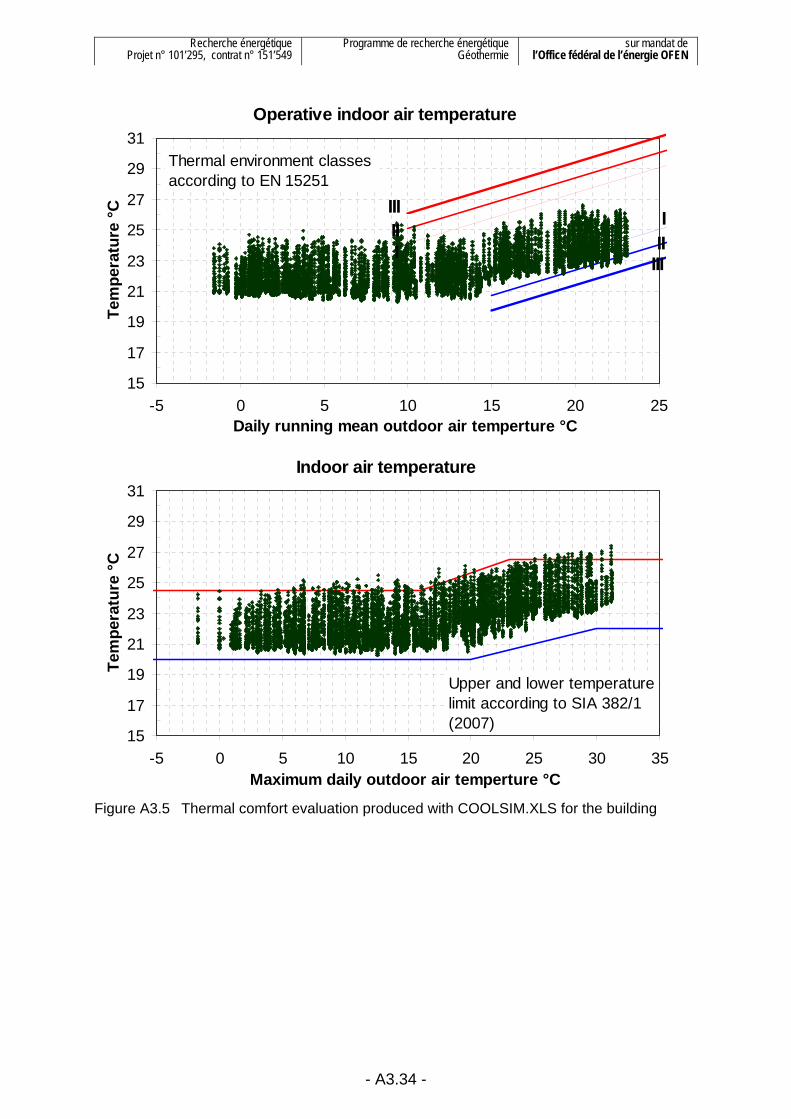
Recherche énergétique Projet n° 101’295, contrat n° 151’549
Programme de recherche énergétique Géothermie
sur mandat de l’Office fédéral de l’énergie OFEN
- A3.34 -
Operative indoor air temperature
IIIIIIIII
III
15
17
19
21
23
25
27
29
31
-5 0 5 10 15 20 25Daily running mean outdoor air temperture °C
Tem
pera
ture
°C
Thermal environment classes according to EN 15251
Indoor air temperature
15
17
19
21
23
25
27
29
31
-5 0 5 10 15 20 25 30 35Maximum daily outdoor air temperture °C
Tem
pera
ture
°C
Upper and lower temperature limit according to SIA 382/1 (2007)
Figure A3.5 Thermal comfort evaluation produced with COOLSIM.XLS for the building

Recherche énergétique Projet n° 101’295, contrat n° 151’549
Programme de recherche énergétique Géothermie
sur mandat de l’Office fédéral de l’énergie OFEN
- A3.35 -
Daily mean temperature
18
20
22
24
26
28
30
49.00 49.25 49.50 49.75 50.0050th operation year
Tem
pera
ture
°C
Fluid warmed temperatureFluid cooled temperatureCeiling surface temperatureOperative temperature
Figure A3.6 Various temperatures evolution produced with COOLSIM.XLS for the building
Operative indoor air temperature
15
17
19
21
23
25
27
29
31
49.00 49.25 49.50 49.75 50.0050th operation year
Tem
pera
ture
°C
Figure A3.7 Operative temperature evolution produced with COOLSIM.XLS for the building

Recherche énergétique Projet n° 101’295, contrat n° 151’549
Programme de recherche énergétique Géothermie
sur mandat de l’Office fédéral de l’énergie OFEN
- A3.36 -
System heat balance mean operation yearkWh/year Auxiliary
heating Total heatElectricity (PAC) 0 demand
18'000 Heat pump PAC heating 74'700(PAC) 74'700
COP 4.1 Heating fraction 100%
56'600Borehole heat Auxiliaryexchangers cooling Total cooling
35'700 0 demandDirect cooling or geocooling 35'700
35'700Cooling fraction 100%
Heating Energy reference areaBuilding annual heating demand 114 MJ/(m2y) 2'360 m2
Maximum heat extraction rate per meter borehole 45 W/m Extraction durationMean heat extraction rate per meter borehole 35 W/m 960 h/yNominal heat extraction rate per meter borehole 33 W/mAnnual extracted energy per meter borehole 33 kWh/m/yearCoolingBuilding annual cooling demand 54 MJ/(m2y)Maximum heat injection rate per meter borehole 38 W/m Injection durationMean heat injection rate per meter borehole 24 W/m 890 h/yAnnual injected energy per meter borehole 21 kWh/m/yearGround heat balanceRatio injected over extracted energy 63% Figure A3.8 Heat balance of the geothermal system produced with COOLSIM.XLS
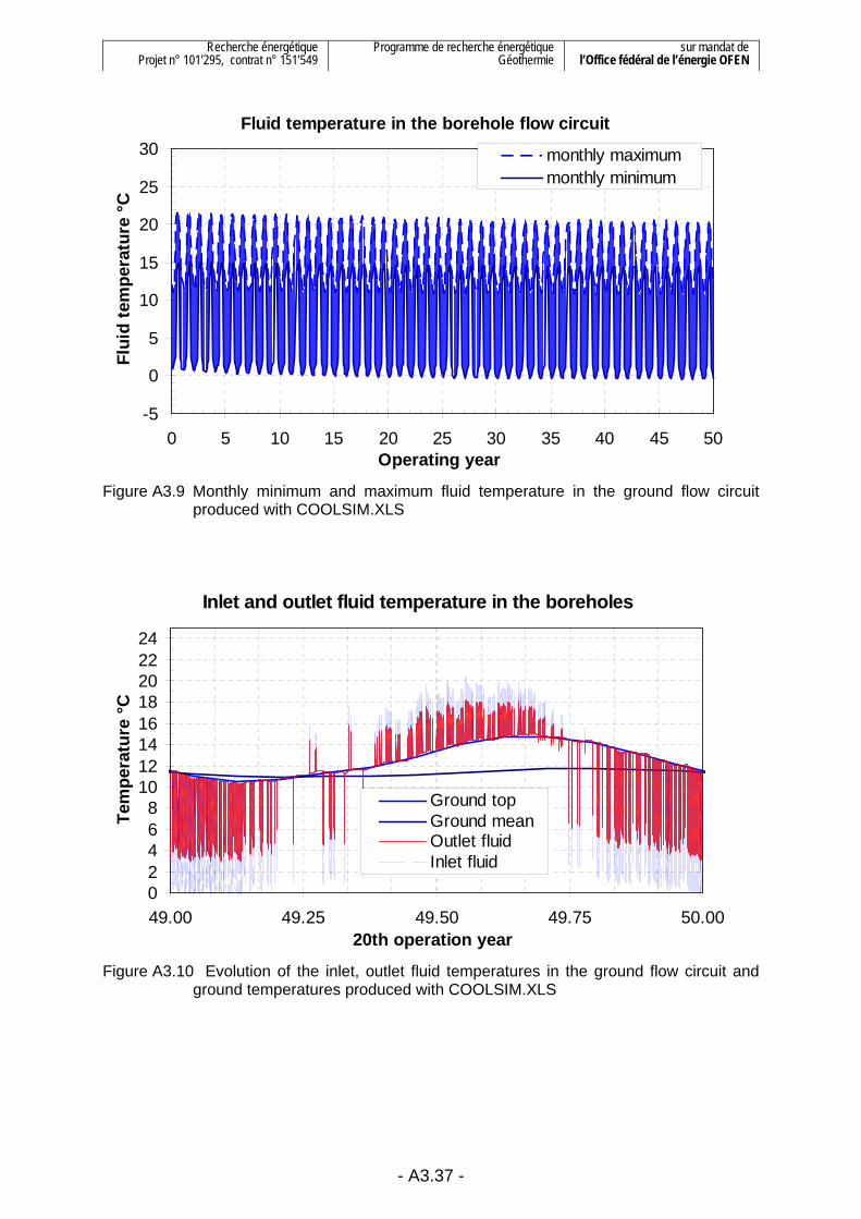
Recherche énergétique Projet n° 101’295, contrat n° 151’549
Programme de recherche énergétique Géothermie
sur mandat de l’Office fédéral de l’énergie OFEN
- A3.37 -
Fluid temperature in the borehole flow circuit
-5
0
5
10
15
20
25
30
0 5 10 15 20 25 30 35 40 45 50Operating year
Flui
d te
mpe
ratu
re °
C
monthly maximummonthly minimum
Figure A3.9 Monthly minimum and maximum fluid temperature in the ground flow circuit
produced with COOLSIM.XLS
Inlet and outlet fluid temperature in the boreholes
02468
1012141618202224
49.00 49.25 49.50 49.75 50.0020th operation year
Tem
pera
ture
°C
Ground topGround meanOutlet fluidInlet fluid
Figure A3.10 Evolution of the inlet, outlet fluid temperatures in the ground flow circuit and
ground temperatures produced with COOLSIM.XLS

Recherche énergétique Projet n° 101’295, contrat n° 151’549
Programme de recherche énergétique Géothermie
sur mandat de l’Office fédéral de l’énergie OFEN
- A3.38 -
Heating and cooling energy demands
-80
-60
-40
-20
0
20
40
60
80
100
49.00 49.25 49.50 49.75 50.0020th operation year
Ther
mal
pow
er k
W
Thermal energy demandCovered by the ground heat system
Figure A3.11 Evolution of heating and cooling powers produced with COOLSIM.XLS Other macros in COOLSIM.XLS allow the user to visualise results of multiple simulations produced with the TRNSED application COOLSIM.

Recherche énergétique Projet n° 101’295, contrat n° 151’549
Programme de recherche énergétique Géothermie
sur mandat de l’Office fédéral de l’énergie OFEN
- A3.39 -
A3.2. Input parameters for the building
A3.2.1. Introduction The input parameters for the building are generated with the TRNBuild programme of the TRNSYS 16.1 package. The TRNBuild programme generates text files that are then read as input data by COOLSIM2. The building must be composed of 6 thermal zones. Two for the building spaces and 4 for the energy distribution system (active concrete plates or floor heating). A3.2.2. INPUT variables The required input variables are 35. They are listed in the required following order: 1. Tambient - outdoor air temperature [°C] 2. Relative humidy ambiente - outdoor air relative humidity [%] 3. Tsky - fictive sky temperature [°C] 4. IT-Horizontal - total incident radiation on horizontal plane [kJ/(hm2)] 5. IT-North - total incident radiation on North façade [kJ/(hm2)] 6. IT-West - total incident radiation on West façade [kJ/(hm2)] 7. IT-East - total incident radiation on East façade [kJ/(hm2)] 8. IT-South - total incident radiation on South façade [kJ/(hm2)] 9. IB-Horizontal - incident beam radiation on horizontal plane [kJ/(hm2)] 10. IB-North - incident beam radiation on North façade [kJ/(hm2)] 11. IB-West - incident beam radiation on West façade [kJ/(hm2)] 12. IB-East - incident beam radiation on East façade [kJ/(hm2)] 13. IB-South - incident beam radiation on South façade [kJ/(hm2)] 14. AI-Horizontal - incident angle of beam radiation for horizontal plane [°] 15. AI-North - incident angle of beam radiation for North façade [°] 16. AI-West - incident angle of beam radiation for West façade [°] 17. AI-East - incident angle of beam radiation for East façade [°] 18. AI-South - incident angle of beam radiation for South façade [°] 19. QTabs3 - heat rate transferred by heat carrier fluid in TABS3 (fictive zone 3) [kJ/h] 20. QTabs4 - heat rate transferred by heat carrier fluid in TABS4 (fictive zone 4) [kJ/h] 21. QTabs5 - heat rate transferred by heat carrier fluid in TABS5 (fictive zone 5) [kJ/h] 22. QTabs6 - heat rate transferred by heat carrier fluid in TABS6 (fictive zone 6) [kJ/h] 23. TVent-Aula - inlet air temperature of ventilation air flow for zone AULA [°C]. Ventilation heat recovery is computed outside of TYPE56 and this air temperature corresponds to inlet air temperature after heat recovery with the AULA heat exchanger in the ventilation system. 24. TVent-Uff - inlet air temperature of ventilation air flow for zone UFFICI [°C]. Ventilation heat recovery is computed outside of TYPE56 and this air temperature corresponds to inlet air temperature after heat recovery with the UFFICI heat exchanger in the ventilation system. 25. Vent-Nott - night cooling ventilation air change rate defined as an infiltration air change in TYPE56 [h-1]. It does also defines a constant infiltration air change rate and a default value of 0.1[h-1] is added to the input value. When no night cooling ventilation is performed, the infiltration air change is then fixed to 0.1[h-1]. When night cooling is realised, 0.1[h-1] should be deducted from the input value, so that the added default value of 0.1[h-1] is cancelled. This is actually done with an EQUATION in the TRNSYS DECK. The magnitude of the night cooling air change rate is defined as a constant user input value in COOLSIM2. 26. Vent-Mec-Aula - air change rate of mechanical ventilation system for zone AULA [h-1]. The magnitude of the air change rate is defined as a constant user input value in

Recherche énergétique Projet n° 101’295, contrat n° 151’549
Programme de recherche énergétique Géothermie
sur mandat de l’Office fédéral de l’énergie OFEN
- A3.40 -
COOLSIM2. Daily operation of the mechanical ventilation system is defined by the schedule V_05_ONOFF (see next section SCHEDULE TYPES). 27. Vent-Mec-Uffici - air change rate of mechanical ventilation system for zone UFFICI [h-1]. The same air change rate magnitude of zone AULA is assigned to zone UFFICI. Daily operation of the mechanical ventilation system is also defined by schedule V_05_ONOFF (see next section SCHEDULE TYPES). 28. ScaleGainsAula - scaling factor for the AULA zone internal heat gains. A scaling factor of 1 corresponds to standard values given in Swiss technical handbook SIA 2024 (2006) for open space office buildings [-] 29. ScaleGainsUffici - scaling factor for the UFFICI zone internal heat gains. A scaling factor of 1 corresponds to standard values given in Swiss technical handbook SIA 2024 (2006) for open space office buildings [-] 30. TCave15 - air temperature of boundary cellar (initially fixed at 15°C) [°C]. If the borehole heat exchangers are lying below the building, this temperature varies and is calculated outside of TYPE56 in function of the building heat losses, the ground surface heat transfer in cellar and the cellar heat losses to the outside environment. If the borehole heat exchangers are located outside of the building this temperature is fixed to a constant temperature defined by the user in COOLSIM2. 31. TCave18 - air temperature of boundary cellar (initially fixed at 18°C) [°C]. The input variable assigned to TCave15 is also assigned to TCave18. 32. IShade - internal shading device factor (0: no shading - 1: maximal shading) [-] 33. EShade - external shading device factor (0: no shading - 1: maximal shading) [-] 34. TintHeat - indoor air temperature limit below which heating is switched on [°C]. This input temperature is only used and defined by the user when the building is simulated without the ground coupled system and the heating distribution system. This parameter is only available to the user in the TRNSED input file BUISIM.TRD 35. TintCool - indoor air temperature limit over which cooling is switched on [°C]. This input temperature is only used and defined by the user when the building is simulated without the ground coupled system and the cooling distribution system. This parameter is only available to the user in the TRNSED input file BUISIM.TRD A3.2.3. OUTPUT variables The required output variables are 27. They are listed in the required following order: 1. Tair-aula - air temperature of zone “aula” 2. Tair-uffici - air temperature of zone “uffici” 3. Tsi1-tabs3 - inside surface temperature of top element TABS3 4. Tsi2-tabs3 - inside surface temperature of bottom element TABS3 5. Tsi1-tabs4 - inside surface temperature of top element TABS4 6. Tsi2-tabs4 - inside surface temperature of bottom element TABS4 7. Tsi1-tabs5 - inside surface temperature of top element TABS5 8. Tsi2-tabs5 - inside surface temperature of bottom element TABS5 9. Tsi1-tabs6 - inside surface temperature of top element TABS6 10. Tsi2-tabs6 - inside surface temperature of bottom element TABS6 11. SQHeat - sum of heating demand for zone “aula” and “uffici” 12. SQCool - sum of cooling demand of zone “aula” and “uffici” 13. SQUA - sum of transmission losses of zone “aula” and “uffici” 14. SQVENT - sum of ventilation gains of zone “aula” and “uffici” 15. SQINF - sum of infiltration gains of zone “aula” and “uffici”
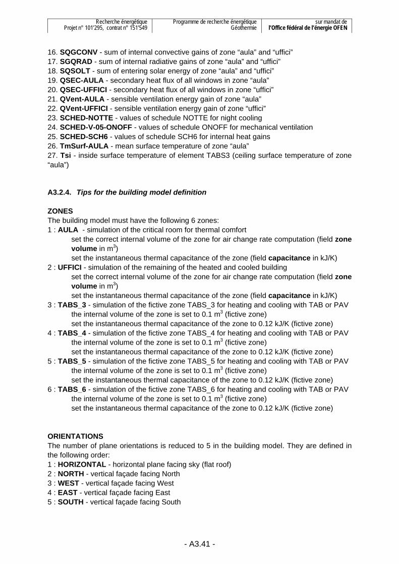
Recherche énergétique Projet n° 101’295, contrat n° 151’549
Programme de recherche énergétique Géothermie
sur mandat de l’Office fédéral de l’énergie OFEN
- A3.41 -
16. SQGCONV - sum of internal convective gains of zone “aula” and “uffici” 17. SGQRAD - sum of internal radiative gains of zone “aula” and “uffici” 18. SQSOLT - sum of entering solar energy of zone “aula” and “uffici” 19. QSEC-AULA - secondary heat flux of all windows in zone “aula” 20. QSEC-UFFICI - secondary heat flux of all windows in zone “uffici” 21. QVent-AULA - sensible ventilation energy gain of zone “aula” 22. QVent-UFFICI - sensible ventilation energy gain of zone “uffici” 23. SCHED-NOTTE - values of schedule NOTTE for night cooling 24. SCHED-V-05-ONOFF - values of schedule ONOFF for mechanical ventilation 25. SCHED-SCH6 - values of schedule SCH6 for internal heat gains 26. TmSurf-AULA - mean surface temperature of zone “aula” 27. Tsi - inside surface temperature of element TABS3 (ceiling surface temperature of zone “aula”) A3.2.4. Tips for the building model definition ZONES The building model must have the following 6 zones: 1 : AULA - simulation of the critical room for thermal comfort
set the correct internal volume of the zone for air change rate computation (field zone volume in m3)
set the instantaneous thermal capacitance of the zone (field capacitance in kJ/K) 2 : UFFICI - simulation of the remaining of the heated and cooled building
set the correct internal volume of the zone for air change rate computation (field zone volume in m3)
set the instantaneous thermal capacitance of the zone (field capacitance in kJ/K) 3 : TABS_3 - simulation of the fictive zone TABS_3 for heating and cooling with TAB or PAV the internal volume of the zone is set to 0.1 m3 (fictive zone) set the instantaneous thermal capacitance of the zone to 0.12 kJ/K (fictive zone) 4 : TABS_4 - simulation of the fictive zone TABS_4 for heating and cooling with TAB or PAV the internal volume of the zone is set to 0.1 m3 (fictive zone) set the instantaneous thermal capacitance of the zone to 0.12 kJ/K (fictive zone) 5 : TABS_5 - simulation of the fictive zone TABS_5 for heating and cooling with TAB or PAV the internal volume of the zone is set to 0.1 m3 (fictive zone) set the instantaneous thermal capacitance of the zone to 0.12 kJ/K (fictive zone) 6 : TABS_6 - simulation of the fictive zone TABS_6 for heating and cooling with TAB or PAV the internal volume of the zone is set to 0.1 m3 (fictive zone) set the instantaneous thermal capacitance of the zone to 0.12 kJ/K (fictive zone) ORIENTATIONS The number of plane orientations is reduced to 5 in the building model. They are defined in the following order: 1 : HORIZONTAL - horizontal plane facing sky (flat roof) 2 : NORTH - vertical façade facing North 3 : WEST - vertical façade facing West 4 : EAST - vertical façade facing East 5 : SOUTH - vertical façade facing South

Recherche énergétique Projet n° 101’295, contrat n° 151’549
Programme de recherche énergétique Géothermie
sur mandat de l’Office fédéral de l’énergie OFEN
- A3.42 -
LAYER TYPE Every layer of material that forms a wall or building element has to be named and the thermal characteristics defined. The layer can be either massive, i.e. its thermal capacity is taken into account in the simulation, or without mass, i.e. only the steady state heat transfer is taken into account. Input data for massive layers: Material Thermal conductivity Thermal capacity Density Name W/(mK) kJ/(hmK) kJ/(kg K) kg/m3 CONCRETE INSULATION COATING … Input data for layers without mass: Layer Thermal resistance Name m2K/W hm2K/kJ AIRLAYER … WALL TYPE Every wall, pavement, roof and building element is formed by the layers that have been defined. They are all named and their stratification defined. Input data for wall types: Building element Stratification defined from
inside to outside U-value
Name LAYER TYPE name
Thickness m
W/(m2K)
EXTERNALWALL CONCRETE INSULATION COATING
0.2 0.3 0.02
… WINDOW TYPE Glazing data, extracted from a data bank, and frame parameters are defined to name the windows. Input data for window types: Window Glazing Frame Name U-value
W/(m2K) g-value -
U-value W/(m2K)
U-value without surface resistances W/(m2K)
…

Recherche énergétique Projet n° 101’295, contrat n° 151’549
Programme de recherche énergétique Géothermie
sur mandat de l’Office fédéral de l’énergie OFEN
- A3.43 -
WALL TYPES IN THE ZONES Definition of the building element in every zone and with their boundary conditions (outside, inside, other zone and so on).
ZONE Type wall
Area[m2]
Area for TRNBUILD
[m2] Category Orien-
-tation Windows
[m2] Windowframes
[%] External walls Internal walls into the same zone Internal walls in contact with other zones Active concrete plates in contact with the external Active concrete plates in contact with other zones Perimeter without Active concrete plates
…
ADDITIONAL INPUT VARIABLES The following inputs have to be created by the user in the following order: 1 : QTABS3 - corresponding to INPUT 19, heat rate transferred by heat carrier fluid in
TABS3. Input to gain type TABS_3, defined as pure convective power. Gain type TABS_3 is
defined in zone TABS_3 as “Other gains”. 2 : QTABS4 - corresponding to INPUT 20, heat rate transferred by heat carrier fluid in
TABS4. Input to gain type TABS_4, defined as pure convective power. Gain type TABS_4 is
defined in zone TABS_4 as “Other Gains”. 3 : QTABS5 - corresponding to INPUT 21, heat rate transferred by heat carrier fluid in
TABS5. Input to gain type TABS_5, defined as pure convective power. Gain type TABS_5 is
defined in zone TABS_5 as “Other Gains”. 4 : QTABS6 - corresponding to INPUT 22, heat rate transferred by heat carrier fluid in
TABS6. Input to gain type TABS_6, defined as pure convective power. Gain type TABS_6 is
defined in zone TABS_6 as “Other Gains”. 5 : TVENT_AULA - corresponding to INPUT 23, inlet air temperature of ventilation air flow
for zone AULA. Input air temperature for ventilation type V_05_AULA.
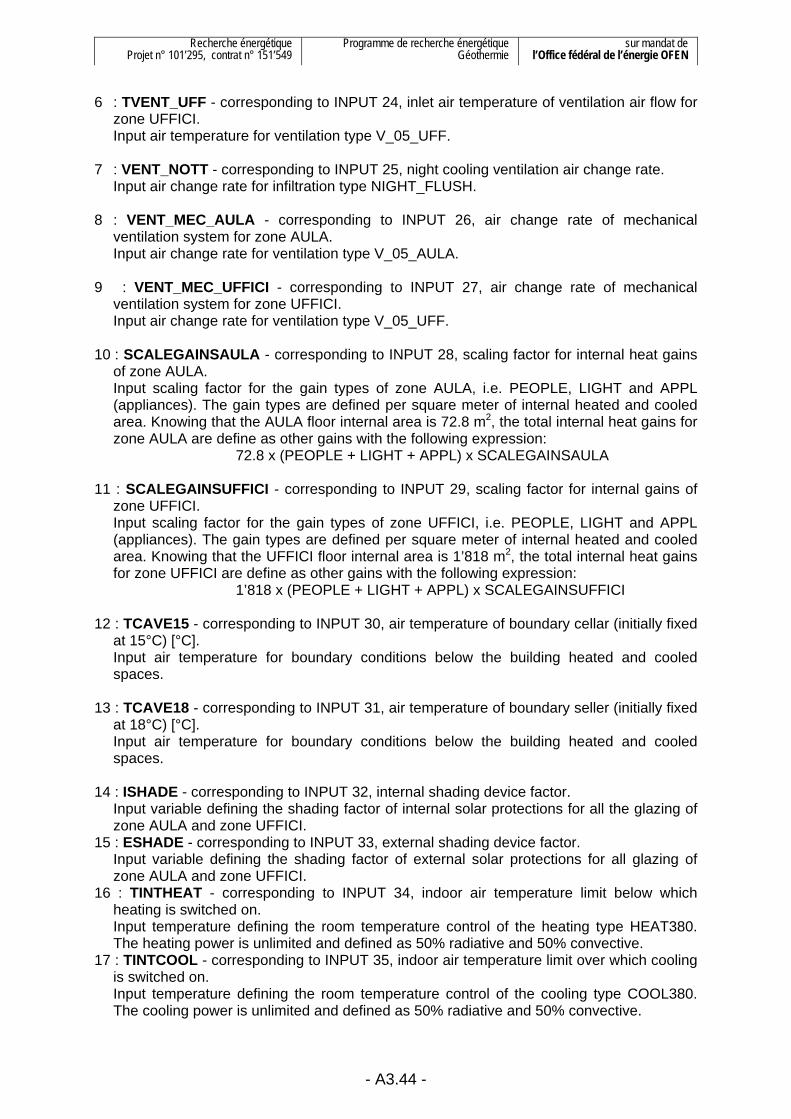
Recherche énergétique Projet n° 101’295, contrat n° 151’549
Programme de recherche énergétique Géothermie
sur mandat de l’Office fédéral de l’énergie OFEN
- A3.44 -
6 : TVENT_UFF - corresponding to INPUT 24, inlet air temperature of ventilation air flow for zone UFFICI.
Input air temperature for ventilation type V_05_UFF. 7 : VENT_NOTT - corresponding to INPUT 25, night cooling ventilation air change rate. Input air change rate for infiltration type NIGHT_FLUSH. 8 : VENT_MEC_AULA - corresponding to INPUT 26, air change rate of mechanical
ventilation system for zone AULA. Input air change rate for ventilation type V_05_AULA. 9 : VENT_MEC_UFFICI - corresponding to INPUT 27, air change rate of mechanical
ventilation system for zone UFFICI. Input air change rate for ventilation type V_05_UFF. 10 : SCALEGAINSAULA - corresponding to INPUT 28, scaling factor for internal heat gains
of zone AULA. Input scaling factor for the gain types of zone AULA, i.e. PEOPLE, LIGHT and APPL
(appliances). The gain types are defined per square meter of internal heated and cooled area. Knowing that the AULA floor internal area is 72.8 m2, the total internal heat gains for zone AULA are define as other gains with the following expression:
72.8 x (PEOPLE + LIGHT + APPL) x SCALEGAINSAULA 11 : SCALEGAINSUFFICI - corresponding to INPUT 29, scaling factor for internal gains of
zone UFFICI. Input scaling factor for the gain types of zone UFFICI, i.e. PEOPLE, LIGHT and APPL
(appliances). The gain types are defined per square meter of internal heated and cooled area. Knowing that the UFFICI floor internal area is 1’818 m2, the total internal heat gains for zone UFFICI are define as other gains with the following expression:
1’818 x (PEOPLE + LIGHT + APPL) x SCALEGAINSUFFICI 12 : TCAVE15 - corresponding to INPUT 30, air temperature of boundary cellar (initially fixed
at 15°C) [°C]. Input air temperature for boundary conditions below the building heated and cooled
spaces. 13 : TCAVE18 - corresponding to INPUT 31, air temperature of boundary seller (initially fixed
at 18°C) [°C]. Input air temperature for boundary conditions below the building heated and cooled
spaces. 14 : ISHADE - corresponding to INPUT 32, internal shading device factor. Input variable defining the shading factor of internal solar protections for all the glazing of
zone AULA and zone UFFICI. 15 : ESHADE - corresponding to INPUT 33, external shading device factor. Input variable defining the shading factor of external solar protections for all glazing of
zone AULA and zone UFFICI. 16 : TINTHEAT - corresponding to INPUT 34, indoor air temperature limit below which
heating is switched on. Input temperature defining the room temperature control of the heating type HEAT380.
The heating power is unlimited and defined as 50% radiative and 50% convective. 17 : TINTCOOL - corresponding to INPUT 35, indoor air temperature limit over which cooling
is switched on. Input temperature defining the room temperature control of the cooling type COOL380.
The cooling power is unlimited and defined as 50% radiative and 50% convective.

Recherche énergétique Projet n° 101’295, contrat n° 151’549
Programme de recherche énergétique Géothermie
sur mandat de l’Office fédéral de l’énergie OFEN
- A3.45 -
INFILTRATION TYPE One infiltration type: 1 : NIGHT_FLUSH is defined for a constant infiltration air change and night cooling [h-1]. It is calculated with input variable Vent-Nott (see INPUT 25): NIGHT_FLUSH = Vent-Nott + 0.1 The inlet air temperature of an infiltration air flow into the building is the outdoor air
temperature. VENTILATION TYPES Two ventilation types: 1 : V_05_AULA is defined for the air change rate of the mechanical ventilation system in
zone AULA [h-1]. It is calculated with input variable VENT_MEC_AULA (see INPUT 26): V_05_AULA = VENT_MEC_AULA The inlet air temperature of the V_05_AULA ventilation type is input variable
TVENT_AULA (see INPUT 23). 2 : V_05_UFF is defined for the air change rate of the mechanical ventilation system in zone
UFFICI [h-1]. It is calculated with input variable VENT_MEC_UFFICI (see INPUT 27): V_05_UFF = VENT_MEC_UFFICI The inlet air temperature of the V_05_UFF ventilation type is input variable TVENT_UFF
(see INPUT 24). HEATING TYPE One heating type: 1 : HEAT380 is defined as a room temperature setting below which heating is switched on. The HEAT380 type is defined with input variable TINTHEAT (see INPUT 34). The required heating power to maintain room temperature at minimum TINTHEAT is not
limited and is defined as 50% radiative and 50% convective. COOLING TYPE One cooling type: 1 : COOL380 is defined as a room temperature setting over which cooling is switched on. The COOL380 type is defined with input variable TINTCOOL (see INPUT 35). The required cooling power to maintain room temperature at maximum TINTCOOL is not
limited. GAIN TYPES Seven gain types: 1 : TABS_3 is defined as a convective thermal power for zone TABS_3 [kJ/h]. The TABS_3 gain type is defined with input variable QTabs3 (see INPUT 19). 2 : TABS_4 is defined as a convective thermal power for zone TABS_4 [kJ/h]. The TABS_4 gain type is defined with input variable QTabs4 (see INPUT 20). 3 : TABS_5 is defined as a convective thermal power for zone TABS_5 [kJ/h]. The TABS_5 gain type is defined with input variable QTabs5 (see INPUT 21).

Recherche énergétique Projet n° 101’295, contrat n° 151’549
Programme de recherche énergétique Géothermie
sur mandat de l’Office fédéral de l’énergie OFEN
- A3.46 -
4 : TABS_6 is defined as a convective thermal power for zone TABS_6 [kJ/h]. The TABS_6 gain type is defined with input variable QTabs6 (see INPUT 22). 5 : PEOPLE is defined as a convective thermal power for persons, according to Swiss
technical handbook SIA 2024 (2006) for open space office buildings. Heat gains, normalised per square meter of internal heated/cooled area, are calculated as follow:
PEOPLE = 20.2 x SC_P_WEEK Where SC_P_WEEK is a weekly schedule defined for building occupation (see next
section SCHEDULE TYPES). 6 : LIGHT is defined as a convective thermal power for lightning, according to Swiss
technical handbook SIA 2024 (2006) for open space office buildings. Heat gains, normalised per square meter of internal heated/cooled area, are calculated as follow:
LIGHT = 45 x SC_L_WEEK Where SC_L_WEEK is a weekly schedule defined for building illumination (see next
section SCHEDULE TYPES). 7 : APPL is defined as a convective thermal power for appliances, according to Swiss
technical handbook SIA 2024 (2006) for open space office buildings. Heat gains, normalised per square meter of internal heated/cooled area, are calculated as follow:
APPL = 28.8 x SC_A_WEEK Where SC_A_WEEK is a weekly schedule defined for electric appliance consumption
(see next section SCHEDULE TYPES). SCHEDULE TYPES Eleven schedule types: 1 : SC_P_WD is a daily schedule defined for internal heat gains caused by people during a
working day [-]. The schedule values are defined as follow for an open space office building: 0h – 7h: 0.00 7h – 8h: 0.18 8h – 9h: 0.36 9h – 10h: 0.52 10h – 11h: 0.70 11h – 12h: 0.71 12h – 13h: 0.36 13h – 14h: 0.52 14h – 16h: 1.00 16h – 17h: 0.36 17h – 18h: 0.18 18h – 24h: 0.00 2 : SC_P_WE is a daily schedule defined for internal heat gains caused by people during the
weekend [-]. The schedule values are defined as follow for an open space office building: 0h – 24h: 0.00 3 : SC_P_WEEK is a weekly schedule defined for internal heat gains caused by people
during a whole week [-]. This schedule, sent as OUTPUT 25, is used in the TRNSYS deck to know when the building is occupied.
The schedule values are defined as follow for an open space office building: Monday to Friday: SC_P_WD (working day schedule for people) Saturday to Sunday: SC_P_WE (weekend schedule for people)

Recherche énergétique Projet n° 101’295, contrat n° 151’549
Programme de recherche énergétique Géothermie
sur mandat de l’Office fédéral de l’énergie OFEN
- A3.47 -
4 : SC_L_WD is a daily schedule defined for internal heat gains caused by illumination during a working day [-].
The schedule values are defined as follow for an open space office building: 0h – 7h: 0.00 7h – 14h: 0.77 14h – 16h: 1.00 16h – 18h: 0.77 18h – 24h: 0.00 5 : SC_L_WE is a daily schedule defined for internal heat gains caused by illumination
during the weekend [-]. The schedule values are defined as follow for an open space office building: 0h – 24h: 0.00 6 : SC_L_WEEK is a weekly schedule defined for internal heat gains caused by illumination
during a whole week [-]. The schedule values are defined as follow for an open space office building: Monday to Friday: SC_L_WD (working day schedule for illumination) Saturday to Sunday: SC_L_WE (weekend schedule for illumination) 7 : SC_A_WD is a daily schedule defined for internal heat gains caused by appliances
during a working day [-]. The schedule values are defined as follow for an open space office building: 0h – 7h: 0.09 7h – 8h: 0.19 8h – 9h: 0.35 9h – 11h: 0.71 11h – 12h: 0.35 12h – 13h: 0.19 13h – 14h: 0.35 14h – 16h: 1.00 16h – 17h: 0.19 17h – 24h: 0.09 8 : SC_A_WE is a daily schedule defined for internal heat gains caused by appliances
during the weekend [-]. The schedule values are defined as follow for an open space office building: 0h – 24h: 0.10 9 : SC_A_WEEK is a weekly schedule defined for internal heat gains caused by appliances
during a whole week [-]. The schedule values are defined as follow for an open space office building: Monday to Friday: SC_A_WD (working day schedule for appliances) Saturday to Sunday: SC_A_WE (weekend schedule for appliances) 10 : V_05_ONOFF is a daily schedule defined for the daily operation of the mechanical
ventilation system [-]. This schedule, sent as OUTPUT 24, conditions INPUT 26 (Vent-Mec_Aula) and 27 (Vent_Mec_Uffici) in the TRNSYS deck.
The schedule values are defined as follow: 0h – 8h: 0.00 8h – 18h: 1.00 18h – 24h: 0.00

Recherche énergétique Projet n° 101’295, contrat n° 151’549
Programme de recherche énergétique Géothermie
sur mandat de l’Office fédéral de l’énergie OFEN
- A3.48 -
11 : NOTTE is a daily schedule to defined a time window when night cooling operation is allowed [-]. This schedule, sent as OUTPUT 23, conditions INPUT 25 in the TRNSYS deck (Vent_Nott).
The schedule values are defined as follow: 0h – 6h: 1.00 6h – 22h: 0.00 22h – 24h: 1.00 OUTPUT VARIABLES The 27 OUTPUT variables are all user defined and created using the following characteristics: 1. Tair-aula - air temperature of zone “aula” Thermal zone: AULA Zone output: NType 1, TAIR – air temperature of zone 2. Tair-uffici - air temperature of zone “uffici” Thermal zone: UFFICI Zone output: NType 1, TAIR – air temperature of zone 3. Tsi1-tabs3 - inside surface temperature of top element TABS3 Thermal zone: TABS_3 Surface output: NType 17, TSI – inside surface temperature Surface 8, TE1AS (surface number and wall type name might be different) 4. Tsi2-tabs3 - inside surface temperature of bottom element TABS3 Thermal zone: TABS_3 Surface output: NType 17, TSI – inside surface temperature Surface 20, TE1AI (surface number and wall type name might be different) 5. Tsi1-tabs4 - inside surface temperature of top element TABS4 Thermal zone: TABS_4 Surface output: NType 17, TSI – inside surface temperature Surface 24, TE1AS (surface number and wall type name might be different) 6. Tsi2-tabs4 - inside surface temperature of bottom element TABS4 Thermal zone: TABS_4 Surface output: NType 17, TSI – inside surface temperature Surface 25, TE1AI (surface number and wall type name might be different) 7. Tsi1-tabs5 - inside surface temperature of top element TABS5 Thermal zone: TABS_5 Surface output: NType 17, TSI – inside surface temperature Surface 27, PA1AS (surface number and wall type name might be different) 8. Tsi2-tabs5 - inside surface temperature of bottom element TABS5 Thermal zone: TABS_5 Surface output: NType 17, TSI – inside surface temperature Surface 29, PA1AI (surface number and wall type name might be different)

Recherche énergétique Projet n° 101’295, contrat n° 151’549
Programme de recherche énergétique Géothermie
sur mandat de l’Office fédéral de l’énergie OFEN
- A3.49 -
9. Tsi1-tabs6 - inside surface temperature of top element TABS6 Thermal zone: TABS_6 Surface output: NType 17, TSI – inside surface temperature Surface 31, PA1AS (surface number and wall type name might be different) 10. Tsi2-tabs6 - inside surface temperature of bottom element TABS6 Thermal zone: TABS_6 Surface output: NType 17, TSI – inside surface temperature Surface 33, PA1AI (surface number and wall type name might be different) 11. SQHeat - sum of heating demand for zone “aula” and “uffici” Thermal zone: AULA e UFFICI Group of zone output: NType 32, SQHEAT – sum of sensible heating demand for group of
zones (positive values) 12. SQCool - sum of cooling demand of zone “aula” and “uffici” Thermal zone: AULA e UFFICI Group of zone output: NType 33, SQCOOL – sum of sensible cooling demand for group of
zones (positive values) 13. SQUA - sum of transmission losses of zone “aula” and “uffici” Thermal zone: AULA e UFFICI Group of zone output: NType 46, SQUA – sum of static transmission losses (UA*dT) for
group of zone 14. SQVENT - sum of ventilation gains of zone “aula” and “uffici” Thermal zone: AULA e UFFICI Group of zone output: NType 36, SQVENT – sum of sensible ventilation energy gains for
group of zones 15. SQINF - sum of infiltration gains of zone “aula” and “uffici” Thermal zone: AULA e UFFICI Group of zone output: NType 35, SQINF – sum of sensible infiltration energy gains for
group of zone 16. SQGCON - sum of internal convective gains of zone “aula” and “uffici” Thermal zone: AULA e UFFICI Group of zone output: NType 38, SQGCON – sum of internal convective gains for group
of zones 17. SGQRAD - sum of internal radiative gains of zone “aula” and “uffici” Thermal zone: AULA e UFFICI Group of zone output: NType 43, SGQRAD – sum of total internal radiative gains for
group of zones 18. SQSOLT - sum of entering solar energy of zone “aula” and “uffici” Thermal zone: AULA e UFFICI Group of zone output: NType 42, SQSOLT – sum of solar radiation transmitted through
windows for group of zones 19. QSEC-AULA - secondary heat flux of all windows in zone “aula” Thermal zone: AULA Zone output: NType 56, QSEC – secondary heat flux of all windows of zone

Recherche énergétique Projet n° 101’295, contrat n° 151’549
Programme de recherche énergétique Géothermie
sur mandat de l’Office fédéral de l’énergie OFEN
- A3.50 -
20. QSEC-UFFICI - secondary heat flux of all windows in zone “uffici” Thermal zone: UFFICI Zone output: NType 56, QSEC – secondary heat flux of all windows of zone 21. QVent-AULA - sensible ventilation energy gain of zone “aula” Thermal zone: AULA Zone output: NType 5, QVENT – sensible ventilation energy gain of zone 22. QVent-UFFICI - sensible ventilation energy gain of zone “uffici” Thermal zone: UFFICI Zone output: NType 5, QVENT – sensible ventilation energy gain of zone 23. SCHED-NOTTE - values of schedule NOTTE for night cooling Thermal zone: AULA Zone output: NType 28, - values of all schedules Schedule: NOTTE 24. SCHED-V-05-ONOFF - values of schedule ONOFF for mechanical ventilation Thermal zone: AULA Zone output: NType 28, - values of all schedules Schedule: V_05_ONOFF 25. SCHED-SCH6 - values of schedule SCH6 for internal heat gains Thermal zone: AULA Zone output: NType 28, - values of all schedules Schedule: SC_P_WEEK 26. TmSurf-AULA - mean surface temperature of zone “aula” Thermal zone: AULA Zone output: NType 24, - weighted mean surface temperature of zone 27. Tsi - inside surface temperature of element TABS3 (ceiling surface temperature of zone “aula”) Thermal zone: AULA Zone output: NType 17, TSI – inside surface temperature Surface 23, TE1AI (surface number and wall type name might be different)

Recherche énergétique Projet n° 101’295, contrat n° 151’549
Programme de recherche énergétique Géothermie
sur mandat de l’Office fédéral de l’énergie OFEN
- A3.51 -
A3.3. References
Klein S. A. et al. (2007) TRNSYS. A Transient System Simulation Program. Version 16.1. Solar Energy Laboratory, University of Wisconsin, Madison, USA.
Merkblatt SIA 2024 (2006) Standard-Nutzungsbedingungen für die Energie- und Gebäudetechnik. Schweizerischer Ingenieur- und Architektenverein, Zürich, Schweiz.
Pahud D. (2007) PILESIM2: Simulation Tool for Heating/Cooling Systems with Energy Piles or multiple Borehole Heat Exchangers. User Manual. ISAAC – DACD – SUPSI, Switzerland.
DIN EN 15251 (2007) Indoor environmental input parameters for design and assessment of energy performance of buildings addressing indoor air quality, thermal environment, lighting and acoustics. Beuth Verlag GmbH, Berlin, Germany
SIA 382/1 (2007) Lüftungs- und Klimaanlagen – Allgemeine Grundlagen und Anforderungen. Schweizerischer Ingenieur- und Architektenverein, Zürich, Schweiz.


Manuale per il raffreddamento di edifici tramite « geocooling » con sonde geotermiche verticali
Rapporto finale D. Pahud e M. Belliardi
Allegato 4
Procedura per determinare i fabbisogni termici dell’edificio
Indice
A4.1. Procedura per la determinazione dei parametri 1
A4.1.1. Fabbisogni di riscaldamento e raffreddamento 1 A4.1.2. Funzionamento del sistema di erogazione per il raffreddamento (Cooling –
ON) 10 A4.1.3. Funzionamento del sistema di erogazione per il raffreddamento e per il
riscaldamento (Cooling - Heating ON) 13 A4.2. Parametri di esclusione 16 A4.3. Riferimenti 17


Recherche énergétique Projet n° 101’295, contrat n° 151’549
Programme de recherche énergétique Géothermie
sur mandat de l’Office fédéral de l’énergie OFEN
- A4.1 -
A4.1. Procedura per la determinazione dei parametri
È qui descritta la procedura per la determinazione dei fabbisogni termici dell’edificio sotto esame. Il TRNSED file utilizzato per l’analisi è BuiSim.
L’edificio analizzato è stato definito nell’allegato 1. È possibile variare alcune caratteristiche chiave, dalle quali conseguono fabbisogni termici differenti e quindi casi-studio diversi.
Le caratteristiche dell’edificio sulle quali agire sono le seguenti:
- due diverse tecniche di erogazione del calore: PAVS o TABS ;
- due differenti percentuali di superfici vetrate: 85% o 50% della superficie totale delle facciate ;
- due tipi diversi di protezioni solari: interne od esterne ;
- due vetri differenti: doppio e triplo.
Sono anche state definite dieci diverse posizioni geografiche : Bologna, Bolzano, Chiasso, Firenze, Genève, Lugano, Milano, Roma, Torino, Zürich.
I fabbisogni termici saranno quindi diversi e dipendenti da numerosi parametri di regolazione descritti nei paragrafi successivi. L’impostazione e la determinazione di questi parametri è sempre comunque finalizzata al raggiungimento e al non superamento delle condizioni limite di benessere interno, sia estive che invernali.
Per semplificare la descrizione dei paragrafi successivi, necessari a spiegare la regolazione dell’edificio, sono state anche usate delle figure e dei grafici riferiti ad un caso pratico specifico, ovvero un edificio con dei TABS, 50% di superfici vetrate, a Chiasso e con delle protezioni solari esterne.
A4.1.1. Fabbisogni di riscaldamento e raffreddamento Questo è il primo step per la determinazione dei parametri di regolazione dell’edificio, che non considerano ancora l’utilizzo dell’impiantistica. I risultati finali di questo paragrafo sono quindi i fabbisogni termici teorici dell’edificio, ovvero la quantità di energia che l’edificio necessita per soddisfare i limiti di benessere (in accordo con la norma SIA 180 (1999)).
Si è proceduto a tappe, in modo ordinato, per avere un metodo coerente e riproducibile per tutti i casi-studio da analizzare.
Sono stati così successivamente descritti i quattro passi necessari per la definizione di questo paragrafo.
Ogni singolo passo è quindi necessario per l’impostazione di un parametro di regolazione dell’edificio; con questo scopo ad ogni step sono state fatte differenti simulazioni per lo stesso edificio e con tutti i parametri costanti, facendo variare solo il valore in esame, in modo da riuscire ad analizzarne l’effetto sull’edificio. Per semplificare e velocizzare i calcoli, sono state create delle tables ad hoc per ogni singolo step; una table è in grado di effettuare delle simulazioni in serie, modificando di volta in volta i parametri chiave che si desidera analizzare. Essendo un processo a tappe, nel passo successivo il valore definito in precedenza dovrà essere fissato manualmente dentro BuiSim.

Recherche énergétique Projet n° 101’295, contrat n° 151’549
Programme de recherche énergétique Géothermie
sur mandat de l’Office fédéral de l’énergie OFEN
- A4.2 -
Il massimo valore di potenza oraria per il riscaldamento che verrà utilizzato come potenza nominale della pompa di calore necessaria per riscaldare l’edificio, è quello che si ottiene alla fine della determinazione di tutti e quattro i parametri descritti nei successivi punti per la regolazione termica dell’edificio (TlimitSummer, IVlimitSummer, IVlimitWinter, TlimitVentHX).
TlimitSummer
Questo parametro definisce il limite oltre il quale si ha il passaggio dalle impostazioni che distinguono il periodo invernale da quello estivo. I due valori successivi (ovvero IVlimitSummer e IVlimitWinter) saranno dipendenti da questa temperatura. Il funzionamento del raffreddamento non è permesso quando le condizioni di temperatura esterna sono inferiori a questo valore, in ogni caso il raffreddamento è permesso solamente se non vi è contemporaneamente la richiesta di riscaldamento (è previsto che non ci sia mai conflitto tra i due).
Rappresenta la temperatura limite media giornaliera dell’aria esterna al di sotto della quale non viene mai attivato il raffreddamento o la ventilazione notturna.
Sulla base di questa temperatura verranno utilizzati i successivi due parametri (cioè IVlimitSummer e IVlimitWinter) per la regolazione delle protezioni solari durante il periodo invernale ed il periodo estivo.
Per poter impostare questo parametro vengono effettuate cinque simulazioni con l’aiuto di una table apposita. Il TlimitSummer varia solitamente da 8°C a 12°C, mentre i valori limite per le protezioni solari sono a questo livello settati a 1000 W/m2 nel periodo invernale e a 100 W/m2 nel periodo estivo. Lo scopo è comunque sempre quello di rimanere dentro i limiti di benessere imposti dalla norma.
Il seguente grafico è stato utilizzato per valutare la dipendenza di questo parametro sulla variazione di fabbisogno termico di riscaldamento e raffreddamento:
0
10
20
30
40
50
60
70
80
5 6 7 8 9 10 11 12 13 14 15Daily outdoor temperature limit for cooling [°C]
Ener
gy [M
J/m
2yea
r]
Heating energyCooling energy
Figura A4.1 : Andamento dei fabbisogni termici invernali ed estivi in funzione della
TlimitSummer.

Recherche énergétique Projet n° 101’295, contrat n° 151’549
Programme de recherche énergétique Géothermie
sur mandat de l’Office fédéral de l’énergie OFEN
- A4.3 -
È possibile notare che con l’aumentare di TlimitSummer i fabbisogni di riscaldamento diminuiscono, mentre quelli di raffreddamento aumentano; è quindi importante trovare un buon compromesso. L’effetto di questo parametro deve poi essere confrontato anche con le condizioni di benessere interno dell’edificio. Il seguente grafico, avente un TlimitSummer impostato a 10°C, mostra come l’andamento delle temperature interne orarie sia ottimamente mantenuto all’interno delle classi di benessere secondo la norma DIN EN 15251 (2007-08).
Operative indoor air temperature
IIIIIIIII
III
1517192123252729313335
-5 0 5 10 15 20 25Daily running mean outdoor air temperture °C
Tem
pera
ture
°C
Thermal environment classes according to EN 15251
Figura A4.2 : Andamento della temperatura operativa dell’aria interna nell’edificio dopo la
regolazione del TlimitSummer, analizzato secondo le classi di benessere definite dalla norma DIN EN 15251 (2007-08).
IVlimitSummer
Questo parametro indica il massimo valore permesso di irraggiamento solare durante l’estate; se l’irraggiamento globale verticale su una delle facciate dell’edificio supera questo valore, vengono inserite le protezioni solari con lo scopo di abbassare il g-value globale delle finestre (vedi allegato 1).
Per poter impostare questo parametro vengono effettuate in serie tre simulazioni, con un IVlimitSummer variabile da 0 W/m2 a 200 W/m2.
Il valore limite per le protezioni solari durante il periodo invernale rimane comunque per adesso fissato a 1000 W/m2, mentre il TlimitSummer trovato nello step precedente deve essere inserito manualmente.
Il seguente grafico è stato utilizzato per valutare la dipendenza di questo parametro sulla variazione di fabbisogno termico di riscaldamento e raffreddamento :
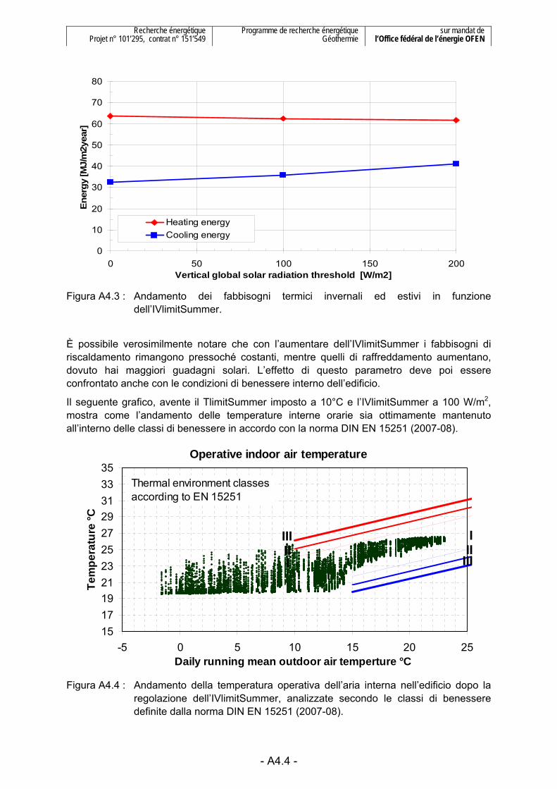
Recherche énergétique Projet n° 101’295, contrat n° 151’549
Programme de recherche énergétique Géothermie
sur mandat de l’Office fédéral de l’énergie OFEN
- A4.4 -
0
10
20
30
40
50
60
70
80
0 50 100 150 200Vertical global solar radiation threshold [W/m2]
Ener
gy [M
J/m
2yea
r]
Heating energyCooling energy
Figura A4.3 : Andamento dei fabbisogni termici invernali ed estivi in funzione
dell’IVlimitSummer.
È possibile verosimilmente notare che con l’aumentare dell’IVlimitSummer i fabbisogni di riscaldamento rimangono pressoché costanti, mentre quelli di raffreddamento aumentano, dovuto hai maggiori guadagni solari. L’effetto di questo parametro deve poi essere confrontato anche con le condizioni di benessere interno dell’edificio.
Il seguente grafico, avente il TlimitSummer imposto a 10°C e l’IVlimitSummer a 100 W/m2, mostra come l’andamento delle temperature interne orarie sia ottimamente mantenuto all’interno delle classi di benessere in accordo con la norma DIN EN 15251 (2007-08).
Operative indoor air temperature
IIIIIIIII
III
1517192123252729313335
-5 0 5 10 15 20 25Daily running mean outdoor air temperture °C
Tem
pera
ture
°C
Thermal environment classes according to EN 15251
Figura A4.4 : Andamento della temperatura operativa dell’aria interna nell’edificio dopo la
regolazione dell’IVlimitSummer, analizzate secondo le classi di benessere definite dalla norma DIN EN 15251 (2007-08).

Recherche énergétique Projet n° 101’295, contrat n° 151’549
Programme de recherche énergétique Géothermie
sur mandat de l’Office fédéral de l’énergie OFEN
- A4.5 -
Da sottolineare il fatto che dopo una serie di differenti edifici simulati, si è notato che è sempre stato definito un valore di 100 W/m2 per l’IVlimitSummer. Dopo aver appunto verificato questo fatto con un elevato numero di simulazioni per differenti casi-studio, si è deciso di prendere per default il valore di 100 W/m2 e non più simulare questo punto.
IVlimitWinter
Questo parametro indica il massimo valore permesso di irraggiamento durante l’inverno; se l’irraggiamento globale verticale in una delle facciate dell’edificio supera questo limite verranno inserite le protezioni solari con lo scopo di abbassare il g-value globale della finestra (vedi allegato 1).
0
10
20
30
40
50
60
70
80
90
100
300 400 500 600 700 800Vertical global solar radiation threshold [W/m2]
Ener
gy [M
J/m
2yea
r]
Heating energyCooling energy
Figura A4.5 : Andamento dei fabbisogni termici invernali ed estivi in funzione
dell’IVlimitWinter.
È possibile verosimilmente notare che solamente il fabbisogno di riscaldamento è sensibile alla variazione dell’IVlimitWinter.
Il seguente grafico confronta l’andamento delle temperature interne orarie con le classi di benessere secondo la norma DIN EN 15251 (2007-08), prendendo un IVlimitWinter pari a 500 W/m2.

Recherche énergétique Projet n° 101’295, contrat n° 151’549
Programme de recherche énergétique Géothermie
sur mandat de l’Office fédéral de l’énergie OFEN
- A4.6 -
Operative indoor air temperature
IIIIIIIII
III
1517192123252729313335
-5 0 5 10 15 20 25Daily running mean outdoor air temperture °C
Tem
pera
ture
°CThermal environment classes according to EN 15251
Figura A4.6 : Andamento delle temperature medie dell’aria interna nell’edificio dopo la
regolazione dell’IVlimitWinter, analizzate secondo le classi di benessere definite dalla norma DIN EN 15251 (2007-08).
Tuttavia per valutare meglio il benessere interno invernale, si è anche analizzato valutando la temperatura massima interna durante l’inverno, con dei limiti imposti in accordo alla norma SIA 180 (1999).
Indoor air temperature
15
17
19
21
23
25
27
29
31
-5 0 5 10 15 20 25 30 35Maximum daily outdoor air temperture °C
Tem
pera
ture
°C
Figura A4.7 : Andamento delle temperature medie dell’aria interna nell’edificio dopo la
regolazione dell’IVlimitWinter.
Si può notare, confrontando entrambi i grafici, che anche durante l’inverno il benessere interno dell’edificio è soddisfatto.
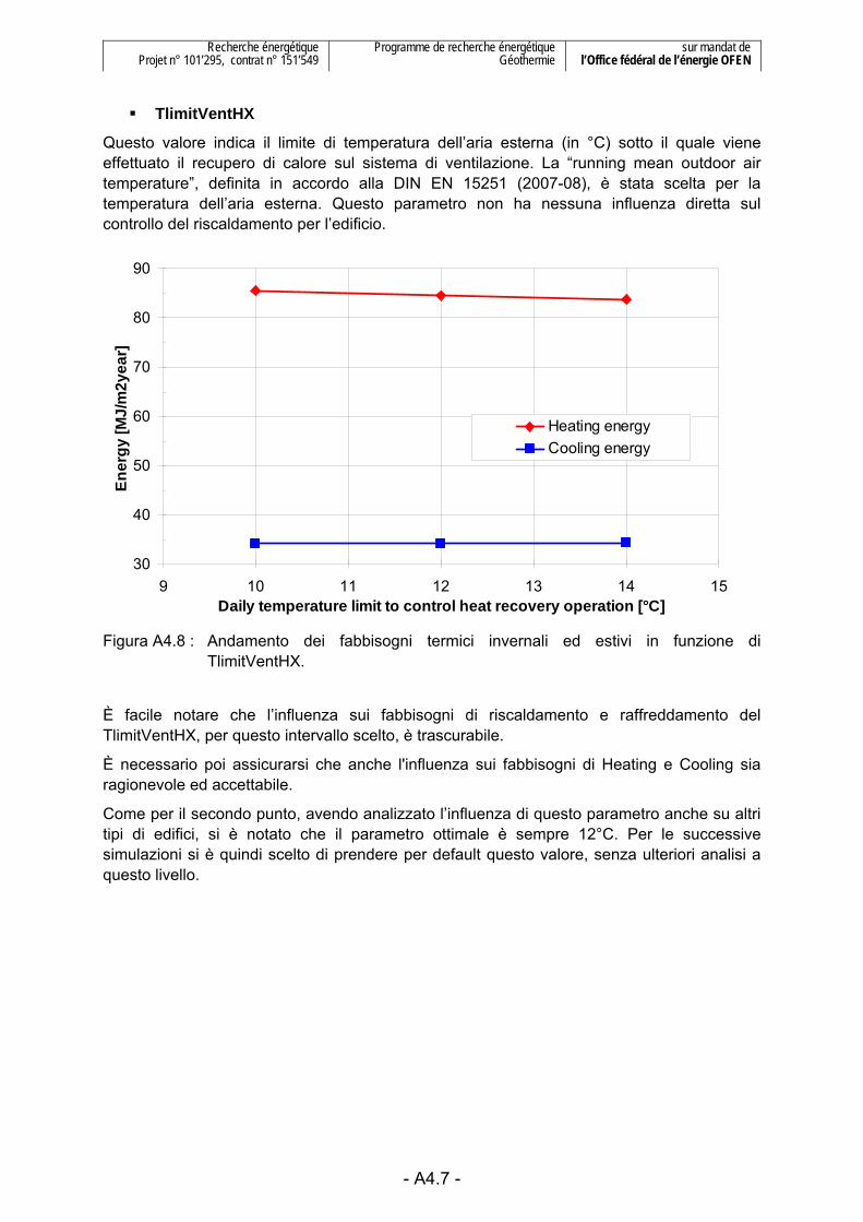
Recherche énergétique Projet n° 101’295, contrat n° 151’549
Programme de recherche énergétique Géothermie
sur mandat de l’Office fédéral de l’énergie OFEN
- A4.7 -
TlimitVentHX
Questo valore indica il limite di temperatura dell’aria esterna (in °C) sotto il quale viene effettuato il recupero di calore sul sistema di ventilazione. La “running mean outdoor air temperature”, definita in accordo alla DIN EN 15251 (2007-08), è stata scelta per la temperatura dell’aria esterna. Questo parametro non ha nessuna influenza diretta sul controllo del riscaldamento per l’edificio.
30
40
50
60
70
80
90
9 10 11 12 13 14 15Daily temperature limit to control heat recovery operation [°C]
Ener
gy [M
J/m
2yea
r]
Heating energyCooling energy
Figura A4.8 : Andamento dei fabbisogni termici invernali ed estivi in funzione di
TlimitVentHX.
È facile notare che l’influenza sui fabbisogni di riscaldamento e raffreddamento del TlimitVentHX, per questo intervallo scelto, è trascurabile.
È necessario poi assicurarsi che anche l'influenza sui fabbisogni di Heating e Cooling sia ragionevole ed accettabile.
Come per il secondo punto, avendo analizzato l’influenza di questo parametro anche su altri tipi di edifici, si è notato che il parametro ottimale è sempre 12°C. Per le successive simulazioni si è quindi scelto di prendere per default questo valore, senza ulteriori analisi a questo livello.

Recherche énergétique Projet n° 101’295, contrat n° 151’549
Programme de recherche énergétique Géothermie
sur mandat de l’Office fédéral de l’énergie OFEN
- A4.8 -
ACRnight
Questo parametro rappresenta il tasso di ricambio d’aria per l’eventuale ventilazione notturna estiva dell’edificio. Un valore tipico per il tasso di ricambio d’aria è 2 (1/h).
La ventilazione notturna viene attivata con le seguenti condizioni :
- temperatura dell’aria esterna è inferiore alla temperatura dell’aria interna ;
- il funzionamento notturno è definito tra le 22h e le 6h ;
- la temperatura di funzionamento dell’aria esterna, definita secondo la norma DIN EN 15251 (2007-08), è maggiore di 15°C.
Questo valore non è stato mai definito fino a questo livello, e si è scelto di impostarlo per default a 0; nel seguente paragrafo verranno fatte alcune considerazioni riguardanti questo parametro.
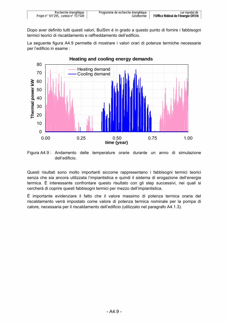
Recherche énergétique Projet n° 101’295, contrat n° 151’549
Programme de recherche énergétique Géothermie
sur mandat de l’Office fédéral de l’énergie OFEN
- A4.9 -
Dopo aver definito tutti questi valori, BuiSim è in grado a questo punto di fornire i fabbisogni termici teorici di riscaldamento e raffreddamento dell’edificio.
La seguente figura A4.9 permette di mostrare i valori orari di potenze termiche necessarie per l’edificio in esame :
Heating and cooling energy demands
0
10
20
30
40
50
60
70
80
0.00 0.25 0.50 0.75 1.00time (year)
Ther
mal
pow
er k
W
Heating demandCooling demand
Figura A4.9 : Andamento delle temperature orarie durante un anno di simulazione
dell’edificio.
Questi risultati sono molto importanti siccome rappresentano i fabbisogni termici teorici senza che sia ancora utilizzata l’impiantistica e quindi il sistema di erogazione dell’energia termica. È interessante confrontare questo risultato con gli step successivi, nei quali si cercherà di coprire questi fabbisogni termici per mezzo dell’impiantistica.
È importante evidenziare il fatto che il valore massimo di potenza termica oraria del riscaldamento verrà impostato come valore di potenza termica nominale per la pompa di calore, necessaria per il riscaldamento dell’edificio (utilizzato nel paragrafo A4.1.3).

Recherche énergétique Projet n° 101’295, contrat n° 151’549
Programme de recherche énergétique Géothermie
sur mandat de l’Office fédéral de l’énergie OFEN
- A4.10 -
A4.1.2. Funzionamento del sistema di erogazione per il raffreddamento (Cooling – ON)
A questo livello è stato attivato il raffreddamento dell’edificio tramite il sistema di erogazione dell’energia di raffreddamento. Per fare ciò è necessario spuntare in BuiSim, all’interno della finestra “Heating and cooling”, il flag “the building is cooled with the following forward fluid temperature”, il quale attiva a sua volta una nuova cella nella quale si inserisce la temperatura di mandata nell’edificio tramite geocooling.
La seguente figura A4.10 mostra la finestra dove è necessario agire per fissare queste impostazioni :
Figura A4.10 : Finestra “Heating and cooling” in BuiSim – attivazione del sistema di
erogazione dell’energia di raffreddamento
Altri due valori da determinare sono la temperatura di attivazione e spegnimento del raffreddamento; questi sono presenti in BuiSim all’interno della finestra “Building” e vengono chiamati “Set point temperature to switch on cooling” e “Set point temperature to switch off cooling”.
È stata creata, per semplificare il procedimento, una table che contiene tre differenti temperature di mandata per il raffreddamento, e quattro condizioni per il set point della temperatura.
Le condizioni di temperatura per il set point del raffreddamento sono differenti nel caso si simuli l’edificio utilizzante dei TABS oppure dei PAVS come sistemi di distribuzione del calore; in particolare, siccome i TABS sono meno reattivi dei PAVS, si è scelto di avere una differenza di temperatura rispettivamente di 1 K e di 1.5 K.
Ecco un esempio che illustra una tipica condizione di set point per il raffreddamento nel caso si utilizzino PAVS oppure TABS :

Recherche énergétique Projet n° 101’295, contrat n° 151’549
Programme de recherche énergétique Géothermie
sur mandat de l’Office fédéral de l’énergie OFEN
- A4.11 -
PAVS
- Set point temperature to switch on cooling : 25.5 °C
- Set point temperature to switch off cooling : 24 °C
TABS
- Set point temperature to switch on cooling : 25.5 °C
- Set point temperature to switch off cooling : 24.5 °C
I punti vengono scelti confrontando i risultati con un limite di 50 ore annue di surriscaldamento (ovvero il numero di ore cui la temperatura dell’aria all’interno dell’edificio è superiore a 26.5°C). Verrà scelto il caso che possiede le temperature di mandata e di set point maggiori, rimanendo sempre al di sotto del vincolo legato alle ore di surriscaldamento.
Ecco un esempio di table usata per questa valutazione :
Figura A4.11 : Table con la definizione delle 12 simulazioni in serie, per la determinazione
dei set-point in funzione della temperatura di mandata del raffreddamento.
Per l’analisi sono state scelte tre temperature di mandata differenti per il raffreddamento (TcoolDesign); in questo esempio sono 19°C , 20°C e 21°C. Se dopo la serie di simulazioni tutte queste temperature risulteranno non adatte per il raffreddamento, a causa di surriscaldamento dei locali o consumi specifici troppo elevati, sarà necessario modificare la table.

Recherche énergétique Projet n° 101’295, contrat n° 151’549
Programme de recherche énergétique Géothermie
sur mandat de l’Office fédéral de l’énergie OFEN
- A4.12 -
Il seguente grafico rappresenta un esempio con i risultati di una serie di simulazioni per il caso base raffreddato con i TABS, evidenziando la dipendenza dalle condizioni di temperatura e dalle ore di surriscaldamento annuali :
0
20
40
60
80
100
23.5 24.0 24.5 25.0 25.5 26.0Set point temperature to switch on cooling [°C]
Hou
rs p
er y
ear T
air >
26.
5°C
[h/y
]
0
20
40
60
80
100
Coo
ling
ener
gy [M
J/(m
2yea
r)]
Tair > 26.5 °CCooling energy
TCoolDesign
21°C
20°C
19°C
19°C20°C21°C
Figura A4.12 : Rappresentazione utilizzata per la determinazione dei set-point e della
temperatura di mandata del raffreddamento ottimale.
In questo caso si è scelto il punto che possiede una temperatura di mandata per il raffreddamento di 21°C (circondato di viola), con la condizione di “set point temperature to switch on cooling” di 25°C. Si nota anche che le ore di surriscaldamento estivo dell’aria interna sono minori di 50 ore annue (limite rappresentato dalla linea rossa sul grafico).
Queste valutazioni sono state fatte nel caso in cui sia o meno presente un sistema di ventilazione meccanica notturna dell’edificio (cosiddetto “night cooling”).
Air change rate for night cooling (ACR night) set to 0 h-1 :
Queste simulazioni non prevedono la ventilazione notturna dell’edificio, ma le condizioni di benessere devono essere soddisfatte esclusivamente con il geocooling.
Air change rate for night cooling (ACR night) set to 2 h-1 :
Queste simulazioni prevedono la ventilazione notturna per abbassare il carico termico estivo dell’edificio; è stato imposto un ricambio d’aria costante pari a 2 h-1 .
Tutti i casi studiati sono stati analizzati senza la ventilazione notturna estiva.

Recherche énergétique Projet n° 101’295, contrat n° 151’549
Programme de recherche énergétique Géothermie
sur mandat de l’Office fédéral de l’énergie OFEN
- A4.13 -
A4.1.3. Funzionamento del sistema di erogazione per il raffreddamento e per il riscaldamento (Cooling - Heating ON)
A questo punto viene anche considerata l’attivazione del sistema di distribuzione per soddisfare i fabbisogni di riscaldamento. Infatti, mentre nel paragrafo precedente i TABS o i PAVS funzionavano solamente in modalità estiva, adesso hanno anche il compito di riscaldare l’edificio in inverno, cercando di mantenere la temperatura interna dell’edificio secondo le prescrizioni di legge sul benessere termico invernale.
Per fare questo è possibile spuntare in BuiSim, all’interno della finestra “Heating and cooling”, il flag “the building is heated with the following heating power”, il quale attiva a sua volta una cella dove è possibile inserire la potenza nominale di riscaldamento e la differenza di temperatura nominale tra l’andata ed il ritorno.
La potenza nominale di dimensionamento, detta “PHeatDesign”, viene letta dal grafico con le potenze orarie risultanti dal paragrafo A4.1.1, una volta determinati tutti i parametri di regolazione dell’edificio.
La seguente figura A4.13 mostra la finestra in BuiSim dove è necessario agire per fissare queste impostazioni :
Figura A4.13 : Finestra “Heating and cooling” in BuiSim – attivazione del sistema di
erogazione per il riscaldamento ed il raffreddamento.
Altri due valori da determinare sono la temperatura di attivazione e spegnimento del riscaldamento, chiamate in BuiSim “Set point temperature to switch on heating” e “Set point temperature to switch off heating”; la differenza di temperatura tra le due condizioni è di 0.5K (valore imposto sia per i TABS che per i PAVS).
Per semplicità è stata anche qui creata una table in modo da effettuare una serie di simulazioni. In questa table sono presenti 3 valori di potenze termiche, ovvero la potenza di dimensionamento nominale ed altre due potenze superiori e inferiori a quest’ultima di 15 kW (20% del valore nominale, per avere una maggiore sensibilità sui risultati). Ognuna di queste potenze viene simulata con una serie di valori per il set-point della temperatura.
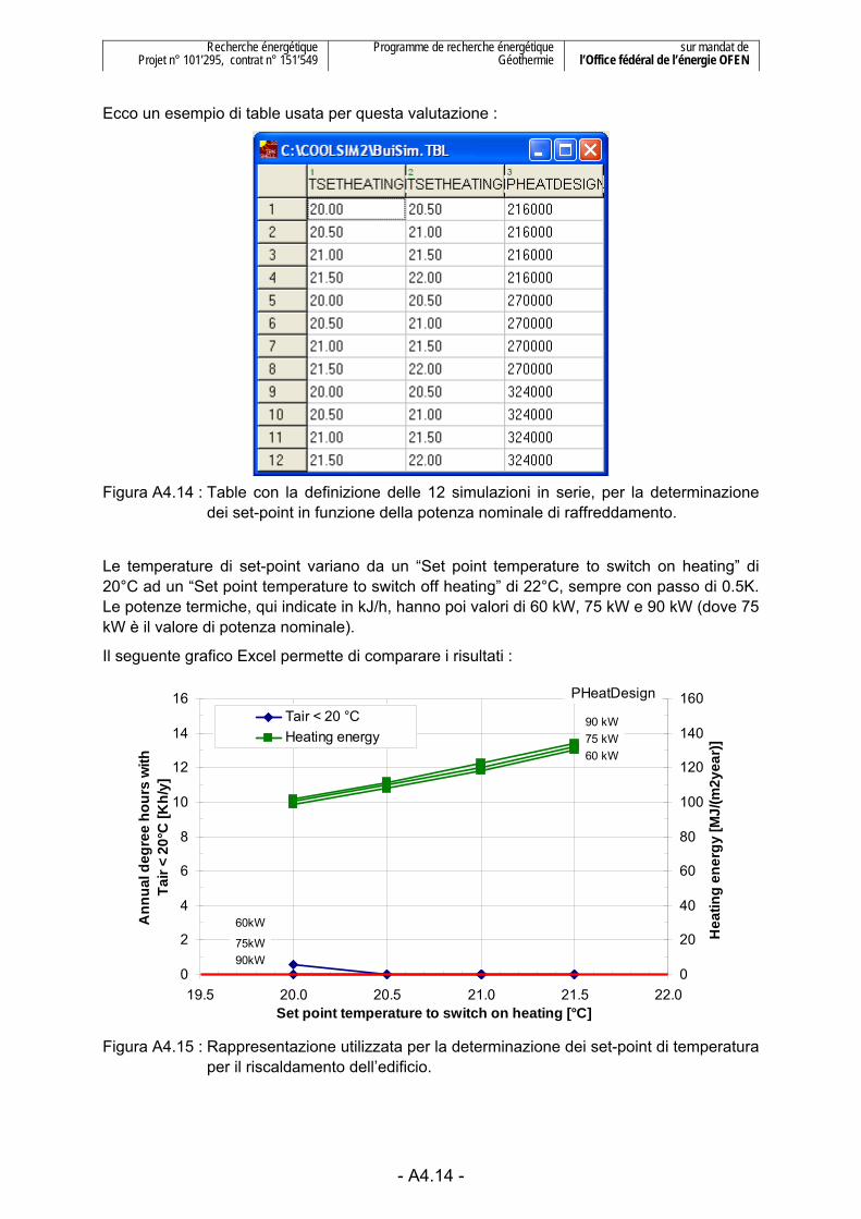
Recherche énergétique Projet n° 101’295, contrat n° 151’549
Programme de recherche énergétique Géothermie
sur mandat de l’Office fédéral de l’énergie OFEN
- A4.14 -
Ecco un esempio di table usata per questa valutazione :
Figura A4.14 : Table con la definizione delle 12 simulazioni in serie, per la determinazione
dei set-point in funzione della potenza nominale di raffreddamento.
Le temperature di set-point variano da un “Set point temperature to switch on heating” di 20°C ad un “Set point temperature to switch off heating” di 22°C, sempre con passo di 0.5K. Le potenze termiche, qui indicate in kJ/h, hanno poi valori di 60 kW, 75 kW e 90 kW (dove 75 kW è il valore di potenza nominale).
Il seguente grafico Excel permette di comparare i risultati :
0
2
4
6
8
10
12
14
16
19.5 20.0 20.5 21.0 21.5 22.0Set point temperature to switch on heating [°C]
Ann
ual d
egre
e ho
urs
with
Ta
ir <
20°C
[Kh/
y]
0
20
40
60
80
100
120
140
160H
eatin
g en
ergy
[MJ/
(m2y
ear)]
Tair < 20 °CHeating energy
PHeatDesign
90 kW75 kW60 kW
90kW75kW
60kW
Figura A4.15 : Rappresentazione utilizzata per la determinazione dei set-point di temperatura
per il riscaldamento dell’edificio.

Recherche énergétique Projet n° 101’295, contrat n° 151’549
Programme de recherche énergétique Géothermie
sur mandat de l’Office fédéral de l’énergie OFEN
- A4.15 -
È necessario prima di tutto verificare che la potenza termica nominale permetta di mantenere la temperatura interna nell’edificio sempre superiore a 20°C.
In questo caso sarebbe sufficiente una temperatura di “set-point to switch on heating” di 20°C, tuttavia la norma SIA 382/1 (2007) indica che la situazione di benessere interno invernale si verifica quando la temperatura dell’aria interna è superiore a 21°C.
Si aumenta così il vincolo sul set-point andando a confrontare i risultati ottenuti sul seguente grafico :
Indoor air temperature
2021222324252627282930
-5 0 5 10 15 20 25 30 35Maximum daily outdoor air temperture °C
Tem
pera
ture
°C
Upper and lower temperature limit according to SIA 382/1 (2007)
Figura A4.16 : Temperature medie dell’aria interna dopo la regolazione di tutti i parametri,
anche quelli legati all’impiantistica, analizzate secondo i limiti definiti dalla norma SIA 382/1 (2007).
In questo esempio il benessere è ottenuto imponendo un “Set point temperature to switch on heating” di 21°C.
A questo punto, una volta che l’impiantistica è entrata in funzione, si può notare che il benessere interno sia estivo che invernale è soddisfatto rimanendo sufficientemente dentro le prescrizioni della norma SIA 382/1 (2007).

Recherche énergétique Projet n° 101’295, contrat n° 151’549
Programme de recherche énergétique Géothermie
sur mandat de l’Office fédéral de l’énergie OFEN
- A4.16 -
A4.2. Parametri di esclusione
In queste analisi vengono simulati molti casi-studio differenti tra di loro, che dipendono dalla posizione geografica, dal tipo di distribuzione di calore, dal tipo di vetro, dalla percentuale di superficie vetrata e dal tipo di protezione solare. Spesso alcune combinazioni di queste condizioni portano ad avere dei problemi di regolazione termica dell’edificio (invernale e/o estiva).
I problemi sono solitamente legati a dei consumi particolarmente elevati rispetto ai fabbisogni iniziali di energia, ad un eccessivo numero di ore di surriscaldamento dell’aria interna, oppure ad un’insensata protezione solare dell’edificio.
Sono stati creati per questo scopo dei criteri di valutazione in modo da poter comparare i diversi casi e capire dove e quali sono i problemi, per poterli poi quantificare e classificare, ed arrivare infine all’accettazione o all’eventuale esclusione di alcuni.
Sono stati previsti principalmente due tipi di indicatori: il WARNING che permette di far riflettere su un eventuale problema ma senza portare all’esclusione del caso, e l’ERROR che indica un effettivo problema in conseguenza del quale è opportuno abbandonare il caso in esame.
I criteri di analisi che portano ad avere un “warning” oppure un “error” sono :
- Il numero di ore di surriscaldamento estivo (cioè T aria interna > 26.5°C) non deve superare le 50 h/a ERROR 1 ;
- Inserimento delle protezioni solari in inverno quando l’irraggiamento solare raggiunge il valore limite di al più 300 W/m2 WARNING 1 ;
- Il rapporto tra i consumi e i fabbisogni di riscaldamento o raffreddamento (vale a dire i fabbisogni teorici senza l’uso dell’impiantistica rispetto a quelli effettivi, ovvero quando entra in gioco anche l’impiantistica) non deve essere maggiore a 2 WARNING 2 ;
- Il rapporto tra i consumi e i fabbisogni di riscaldamento o raffreddamento non deve essere maggiore a 3 ERROR 2 .
La seguente tabella riassume ed elenca i differenti criteri di analisi :
Condizione WARNING 1 ERROR 1 WARNING 2 ERROR 2
Tair > 26.5°C N°ore > 50 h/y
IV limit Winter ≤ 300 W/m2
consumi ≥ 2 fabbisogni (riscald. o raffredd.)
consumi ≥ 3 fabbisogni (riscald. o raffredd.)
Figura A4.17 : Rappresentazione delle condizioni di attenzione e di esclusione con i relativi criteri limite da analizzare.

Recherche énergétique Projet n° 101’295, contrat n° 151’549
Programme de recherche énergétique Géothermie
sur mandat de l’Office fédéral de l’énergie OFEN
- A4.17 -
Solitamente tutti i casi studio che portano ad avere uno o più ERROR non vengono più considerati nelle successive analisi (ovvero le simulazioni dell’impianto geotermico con COOLSIM2); i casi che presentano dei WARNING invece non sono esclusi a priori, ma viene posta su di essi particolare attenzione e vengono fatte delle singole riflessioni.
A4.3. Riferimenti
SIA 382/1 (2007) Lüftungs- und Klimaanlagen – Allgemeine Grundlagen und Anforderungen. Schweizerischer Ingenieur- und Architektenverein, Zürich, Schweiz.
SIA 180 (1999) Isolamento termico e protezione contro l’umidità degli edifici. Società Svizzera degli Ingegneri e degli Architetti, Zurigo, Svizzera.
DIN EN 15251 (2007-08) Indoor environmental input parameters for design and assessment of Energy performance of buildings addressing indoor air quality, thermal environment, lighting and acoustics. Deutsches Institut für Normung, Berlin, Germany.


Manuale per il raffreddamento di edifici tramite « geocooling » con sonde geotermiche verticali
Rapporto finale D. Pahud e M. Belliardi
Allegato 5
Procedura per dimensionare l’impianto geotermico
Indice
A5.1. Introduzione al metodo 1
A5.1.1. Impostazioni dei parametri in COOLSIM2 1 A5.1.2. Impostazione della table 6
A5.2. Risultati e analisi 8


Recherche énergétique Projet n° 101’295, contrat n° 151’549
Programme de recherche énergétique Géothermie
sur mandat de l’Office fédéral de l’énergie OFEN
- A5.1 -
A5.1. Introduzione al metodo
È qui descritto il metodo con il quale si è arrivati a determinare i diversi dimensionamenti dei campi di sonde geotermiche dei differenti casi-studio analizzati.
Il programma utilizzato per questa valutazione è COOLSIM2.
Dapprima vengono inseriti i vari parametri climatici, per passare poi a quelli legati all’edificio e all’impiantistica (alcuni già precedentemente determinati con BuiSim), e per finire con l’aggiunta di quelli che definiscono il campo di sonde e le proprietà termiche del terreno.
Siccome COOLSIM2 genera una sola simulazione con i parametri inseriti, verrà poi creata una table ad hoc, contenente un intervallo variabile di tre parametri; in questo modo è possibile lanciare una serie di simulazioni ed avere più risultati da analizzare.
A5.1.1. Impostazioni dei parametri in COOLSIM2
L’interfaccia di COOLSIM2 prevede una serie di finestre selezionabili, riguardanti varie tematiche necessarie per il dimensionamento; all’interno di ognuna di queste finestre ci sono i parametri da definire.
Le finestre sono 6 e sono selezionabili nella parte superiore del programma, ecco un’immagine che ne descrive l’ordine e l’interfaccia :
Figura A5.1 : Interfaccia ed ordine delle finestre di dialogo per l’inserimento dei parametri in
COOLSIM2.
Verranno adesso descritti nel dettaglio i parametri da inserire per ogni finestra, tenendo presente che tutti i parametri legati all’edificio ed ai suoi fabbisogni termici sono già stati definiti e determinati nell’allegato 4.
Simulation and location
Figura A5.2 : Finestra di dialogo “Simulation and location” in COOLSIM2.
È possibile in questa finestra inserire i valori temporali e geografici per la simulazione, quali l’inizio del periodo della simulazione, la durata della simulazione e la locazione geografica.
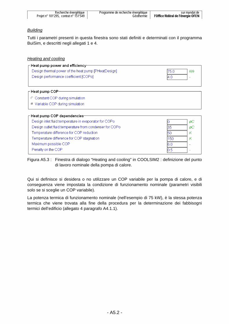
Recherche énergétique Projet n° 101’295, contrat n° 151’549
Programme de recherche énergétique Géothermie
sur mandat de l’Office fédéral de l’énergie OFEN
- A5.2 -
Building
Tutti i parametri presenti in questa finestra sono stati definiti e determinati con il programma BuiSim, e descritti negli allegati 1 e 4.
Heating and cooling
Figura A5.3 : Finestra di dialogo “Heating and cooling” in COOLSIM2 : definizione del punto
di lavoro nominale della pompa di calore.
Qui si definisce si desidera o no utilizzare un COP variabile per la pompa di calore, e di conseguenza viene impostata la condizione di funzionamento nominale (parametri visibili solo se si sceglie un COP variabile).
La potenza termica di funzionamento nominale (nell’esempio di 75 kW), è la stessa potenza termica che viene trovata alla fine della procedura per la determinazione dei fabbisogni termici dell’edificio (allegato 4 paragrafo A4.1.1).

Recherche énergétique Projet n° 101’295, contrat n° 151’549
Programme de recherche énergétique Géothermie
sur mandat de l’Office fédéral de l’énergie OFEN
- A5.3 -
Figura A5.4 : Finestra di dialogo “Heating and cooling” in COOLSIM2 : definizione delle
differenze di temperatura nominale della pompa di calore, e della temperatura di mandata del geocooling con il relativo coefficiente di scambio termico dello scambiatore di calore.
Per il geocooling la temperatura di mandata nominale viene anch’essa determinata nell’allegato 4, in particolare nel paragrafo A4.1.2 , mentre il coefficiente di scambio termico dello scambiatore di calore per il geocooling, è stato impostato in questo esempio a 30 kW/K (valore ritenuto plausibile in base all’esperienza).
Interface ground-building
Figura A5.5 : Finestra di dialogo “Interface ground-building” in COOLSIM2.
Viene qui definita l’ubicazione del campo di sonde geotermiche, che può essere all’esterno oppure sotto una costruzione. Siccome le sonde, ed in particolare le connessioni orizzontali, dipendono anche dalle condizioni di temperatura superficiali, è necessario definire le condizioni e le caratteristiche del locale sovrastante, e quindi la lunghezza totale dei collegamenti orizzontali (LCOEPF).
In questo studio si è scelto di definire questa lunghezza come il numero di sonde moltiplicato per la distanza media tra di loro (parametri chiamati rispettivamente N1 e BPILE, vedi punto seguente), ne risulta quindi che :
LCOEPF = N1 x BPILE

Recherche énergétique Projet n° 101’295, contrat n° 151’549
Programme de recherche énergétique Géothermie
sur mandat de l’Office fédéral de l’énergie OFEN
- A5.4 -
Ground heat exchanger
Figura A5.6 : Finestra di dialogo “Ground heat exchanger” in COOLSIM2. In questa finestra si definiscono le caratteristiche delle sonde e del campo di sonde. Sarebbe possibile inserire in COOLSIM2 fino a 6 tipi differenti di sonde, tuttavia in questo studio si considera sempre che tutte le sonde siano uguali tra di loro, con lo stesso diametro, profondità e resistenze termiche (valori cerchiati in rosso).
Alla fine della finestra è inoltre necessario definire le caratteristiche del campo di sonde, con la distanza media ed il numero di sonde idraulicamente collegate in serie.
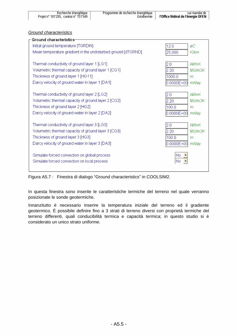
Recherche énergétique Projet n° 101’295, contrat n° 151’549
Programme de recherche énergétique Géothermie
sur mandat de l’Office fédéral de l’énergie OFEN
- A5.5 -
Ground characteristics
Figura A5.7 : Finestra di dialogo “Ground characteristics” in COOLSIM2.
In questa finestra sono inserite le caratteristiche termiche del terreno nel quale verranno posizionate le sonde geotermiche.
Innanzitutto è necessario inserire la temperatura iniziale del terreno ed il gradiente geotermico. È possibile definire fino a 3 strati di terreno diversi con proprietà termiche del terreno differenti, quali conducibilità termica e capacità termica; in questo studio si è considerato un unico strato uniforme.

Recherche énergétique Projet n° 101’295, contrat n° 151’549
Programme de recherche énergétique Géothermie
sur mandat de l’Office fédéral de l’énergie OFEN
- A5.6 -
A5.1.2. Impostazione della table L’idea che si è seguita per ottenere il dimensionamento è quella di lanciare, utilizzando una table, una serie di simulazioni per lo stesso caso-studio di edificio; è così possibile far variare in modo sistematico il numero di sonde e la conducibilità termica del terreno. Si ottengono in questo modo molteplici risultati che, opportunamente studiati anche grazie a dei grafici Excel, potranno dare numerose informazioni utili tra cui il dimensionamento dell’impianto geotermico.
Sono qui elencate e descritte le due scelte di variazione dei parametri per COOLSIM2.
Variazione della conducibilità termica del terreno
La serie di simulazioni effettuata ha lo scopo di valutare il dimensionamento degli impianti in base a differenti conducibilità termiche del terreno. Vengono infatti studiati i risultati del dimensionamento per le seguenti conducibilità del terreno : 1.5 W/(mK), 2 W/(mK), 2.5 W/(mK), 3 W/(mK), 3.5 W/(mK), 4 W/(mK).
Una volta ottenuti i risultati sarà possibile scegliere il valore più appropriato per l’impianto in esame, ed inoltre sarà anche interessante osservare la sensibilità del dimensionamento in funzione di questi parametri.
Variazione del numero di sonde
Per poter rendere la table la più generica possibile, le simulazioni vengono fatte con un numero di sonde che varia solitamente da un minimo di 10 ad un massimo di 30 sonde, e comunque con un numero fisso di 7 simulazioni (ad esempio 10, 12, 14, 17, 20, 24, 30, sonde).
In base alle differenti scelte di progetto per ogni caso-studio, legate principalmente all’edificio, all’impiantistica e alle condizioni limite di temperatura, sarà possibile trovare la soluzione per il dimensionamento geotermico in questo intervallo di valori.
Questo intervallo è stato adattato a questo edificio e ad una profondità delle sonde di 100 m ciascuna; se si aumenta la profondità sarà opportuno diminuire conseguentemente il numero di sonde.
Un terzo valore necessario da inserire, ma comunque sempre dipendente dal numero di sonde, è la lunghezza dei collegamenti orizzontali; questa lunghezza è stata infatti definita come il numero di sonde per la distanza media tra di loro (vedi paragrafo A5.1.1 punto “interface building” ).
Ne risulta quindi che con le 7 simulazioni per la dipendenza dal numero di sonde, e le 6 per la conducibilità termica del terreno, si ottengono un totale di 42 simulazioni in serie da effettuare con COOLSIM2 per il dimensionamento geotermico.
La seguente figura rappresenta un esempio di table usata per una serie di simulazioni necessarie per il dimensionamento del campo di sonde (avente una distanza media delle sonde di 8 m ed una profondità di 100 m ciascuna).
Da notare (evidenziato in rosso) che la conducibilità termica LG1 è espressa in (kJ/h)/(mK) , è quindi necessario moltiplicare i valori in W/(mK) per 3.6 (ks/h).

Recherche énergétique Projet n° 101’295, contrat n° 151’549
Programme de recherche énergétique Géothermie
sur mandat de l’Office fédéral de l’énergie OFEN
- A5.7 -
Figura A5.8 : Esempio di table utilizzata per la serie di 42 simulazioni con COOLSIM2.
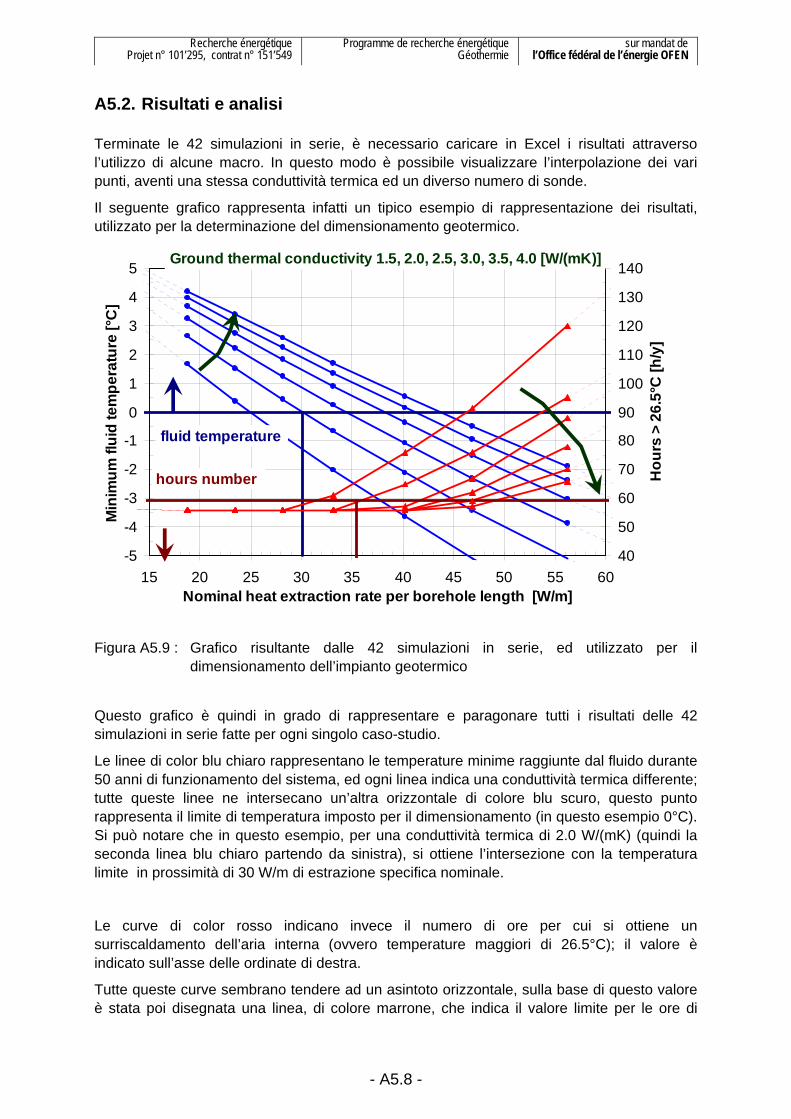
Recherche énergétique Projet n° 101’295, contrat n° 151’549
Programme de recherche énergétique Géothermie
sur mandat de l’Office fédéral de l’énergie OFEN
- A5.8 -
A5.2. Risultati e analisi
Terminate le 42 simulazioni in serie, è necessario caricare in Excel i risultati attraverso l’utilizzo di alcune macro. In questo modo è possibile visualizzare l’interpolazione dei vari punti, aventi una stessa conduttività termica ed un diverso numero di sonde.
Il seguente grafico rappresenta infatti un tipico esempio di rappresentazione dei risultati, utilizzato per la determinazione del dimensionamento geotermico.
-5
-4
-3
-2
-1
0
1
2
3
4
5
15 20 25 30 35 40 45 50 55 60Nominal heat extraction rate per borehole length [W/m]
Min
imum
flui
d te
mpe
ratu
re [°
C]
40
50
60
70
80
90
100
110
120
130
140
Hou
rs >
26.
5°C
[h/y
]
Ground thermal conductivity 1.5, 2.0, 2.5, 3.0, 3.5, 4.0 [W/(mK)]
fluid temperature
hours number
Figura A5.9 : Grafico risultante dalle 42 simulazioni in serie, ed utilizzato per il
dimensionamento dell’impianto geotermico
Questo grafico è quindi in grado di rappresentare e paragonare tutti i risultati delle 42 simulazioni in serie fatte per ogni singolo caso-studio.
Le linee di color blu chiaro rappresentano le temperature minime raggiunte dal fluido durante 50 anni di funzionamento del sistema, ed ogni linea indica una conduttività termica differente; tutte queste linee ne intersecano un’altra orizzontale di colore blu scuro, questo punto rappresenta il limite di temperatura imposto per il dimensionamento (in questo esempio 0°C). Si può notare che in questo esempio, per una conduttività termica di 2.0 W/(mK) (quindi la seconda linea blu chiaro partendo da sinistra), si ottiene l’intersezione con la temperatura limite in prossimità di 30 W/m di estrazione specifica nominale.
Le curve di color rosso indicano invece il numero di ore per cui si ottiene un surriscaldamento dell’aria interna (ovvero temperature maggiori di 26.5°C); il valore è indicato sull’asse delle ordinate di destra.
Tutte queste curve sembrano tendere ad un asintoto orizzontale, sulla base di questo valore è stata poi disegnata una linea, di colore marrone, che indica il valore limite per le ore di

Recherche énergétique Projet n° 101’295, contrat n° 151’549
Programme de recherche énergétique Géothermie
sur mandat de l’Office fédéral de l’énergie OFEN
- A5.9 -
surriscaldamento estive. Sempre basandosi su questo esempio, per il caso di una conducibilità termica pari a 2 W/(mK) (quindi la seconda linea rossa partendo dall’alto), si può notare che l’intersezione si ottiene a circa 35 W/m di estrazione specifica nominale.
Nei calcoli successivi verrà utilizzato, per il dimensionamento del sistema, il minore di questi due valori, in modo da rimanere conservativi e soprattutto non penalizzare il riscaldamento od il raffreddamento.
È a questo punto possibile, grazie a dei calcoli appositi, ottenere il dimensionamento del sistema, in termini di numero di sonde e portata di fluido per sonda.
La seguente immagine mostra i risultati per il caso in esame, e per una conduttività termica del terreno sempre di 2 W/(mK) (da inserire manualmente nella cella di color giallo).
System sizing with ground thermal conductivity of 2 W/(mK)
Specific nominal heat extraction rate based on:Winter sizing with Tfluid > 0 °C 30 W/mSummer sizing with (Nhours>26.5°C) < 59 h/y 35 W/m
System sizing 30 W/m
Nominal heat extraction rate 56.2 kWTotal borehole length 1869 mBorehole depth 100 mBorehole number 19 -
Total flow rate in the ground circuit heating 14 m3/hgeocooling 21 m3/h
Flow rate per borehole with 2 bore in seriesheating 1.5 m3/hgeocooling 2.3 m3/h
Figura A5.10 : Esempio di table utilizzata per le 42 simulazioni in serie con il COOLSIM2.
Grazie a questi risultati è possibile ottenere il dimensionamento per il caso in esame; in questo esempio il numero di sonde calcolato e necessario per soddisfare i fabbisogni sia estivi che invernali, senza violare i limiti imposti di temperatura minima del fluido termovettore e surriscaldamento dei locali, è di 19 sonde da 100 m di profondità, con una distanza media di 8 metri tra di loro.
La lunghezza totale delle sonde viene calcolata basandosi sulla potenza nominale di estrazione (in questo esempio 56.2 kW), che deriva dal COP di 4 alle condizioni nominali B0W35 ed dalla potenza nominale di riscaldamento (valutata con il BUISIM, allegato 4 paragrafo A4.1.1, 75 kW per il caso in esempio).
Dividendo la potenza nominale di estrazione per il minimo valore di potenza specifica di estrazione secondo i due criteri di dimensionamento invernali ed estivi, si ottiene la lunghezza totale di perforazione.

Recherche énergétique Projet n° 101’295, contrat n° 151’549
Programme de recherche énergétique Géothermie
sur mandat de l’Office fédéral de l’énergie OFEN
- A5.10 -
A questo punto, una volta determinato il numero di sonde necessarie per il caso-studio, non rimane che simulare un’ultima volta con COOLSIM2, senza più la table ma inserendo il numero esatto di sonde, di collegamenti orizzontali, di conduttività termica del terreno ed eventualmente di sonde in serie (necessario per regolare la portata per sonda). Quest’ultima procedura è necessaria in modo da poter aggiornare il file Excel con gli esatti valori di dimensionamento.
Related Documents