1 IDENTIFICATION OF MANGROVE ZONATION AND SUCCESSION PATTERN IN THE DELTAIC ISLANDS BY REMOTE SENSING AND GIS TECHNIQUE A CASE STUDY ON LOTHIAN AND PRENTICE ISLAND, SUNDARBAN, WEST BENGAL SUBMITED BY BISWAJIT DAS UNDER GUIDENCE OF Dr. JATISANKAR BANDYOPADHYAY DEPERTMENT OF REMOTE SENSING & GIS VIDYASAGAR UNIVERSITY, MIDNAPURE-721102 IN 2013 GEO-SPATIAL ASSESSMENT OF AGRICULTURAL DROUGHT BY REMOTE SENSING & GIS TECNNIQUE (A CASE STUDY OF BANKURA, WEST BENGAL)

Welcome message from author
This document is posted to help you gain knowledge. Please leave a comment to let me know what you think about it! Share it to your friends and learn new things together.
Transcript
1
IDENTIFICATION OF MANGROVE ZONATION AND SUCCESSION PATTERN IN THE DELTAIC ISLANDS BY REMOTE
SENSING AND GIS TECHNIQUE
A CASE STUDY ON LOTHIAN AND PRENTICE ISLAND, SUNDAR BAN, WEST BENGAL
SUBMITED
BY
BISWAJIT DAS
UNDER GUIDENCE
OF
Dr. JATISANKAR BANDYOPADHYAY
DEPERTMENT OF REMOTE SENSING & GIS
VIDYASAGAR UNIVERSITY,
MIDNAPURE-721102
IN 2013
GEO-SPATIAL ASSESSMENT OF AGRICULTURAL DROUGHT BY REMOTE SENSING & GIS TECNNIQUE
(A CASE STUDY OF BANKURA, WEST BENGAL)
2
GEO-SPATIAL ASSESSMENT AGRICULTURAL DROUGHT BY REMOTE SENSING & GIS TECNNIQUE
(A CASE STUDY OF BANKURA, WEST BENGAL)
SUBMITED
BY
BISWAJIT DAS
UNDER GUIDENCE
OF
Dr. JATISANKAR BANDYOPADHYAY
DEPERTMENT OF REMOTE SENSING & GIS
VIDYASAGAR UNIVERSITY
MIDNAPURE-721102
2013
3
ACKNOWLEDGEMENT
I would like to thanks Dr. Jatisankar Bandyopadhyay (Faculty of
Remote Sensing & GIS dept., Vidyasagar University), Dr. Abhisek Chakraborty
(Faculty of Remote Sensing & GIS dept., Vidyasagar University) and Dr.
Sikhendra Kishor De (Visiting Faculty, Retired Director G.S.I) for their
valuable thought and knowledge given throughout the study of M.Sc. course
I wish to express my deep sense of gratitude to Mr. Ratnadeep Ray
(Faculty of Remote Sensing & GIS dept., Vidyasagar University) for his advice,
support and assistance throughout my dissertation work.
Finally, yet importantly, I would like to express my heartfelt thanks to my
beloved parents for their blessings, my friends/classmates for their help and
wishes for the successful completion of this project work.
……………………………………
Biswajit Das
Dept of Remote Sensing and GIS
Vidyasagar University
4
ABSTRACT
Climate has always been a dynamic entity affecting natural systems through the
consequence of its variability and change. Agriculture is the most vulnerable and sensitive
sector that is seriously affected by the impact of climate variability and change, which is
usually manifested through rainfall variability and recurrent drought. Drought is the most
complex but least understood of all natural hazards. Low rainfall and fall in agricultural
production has mainly caused droughts.
In recent years, Geospatial techniques have played a key role in studying different
types of hazards either natural or manmade. This study stresses upon the use of RS & GIS in
the field of drought risk assessment. In Bankura District, West Bengal agricultural drought
and crop failure have been common, and farmers inhabiting the area experience extreme
temporal and spatial variability of rainfall in cropping season with frequent and longer dry
spells. This makes them vulnerable to the risk of agricultural drought. Thus, in order to adapt
and/or mitigate the impact of agricultural drought, agricultural drought assessment has to
form one dimension of research to be done whereas the use of remote sensing and GIS
techniques provides wide scope in drought risk detection and mapping. Consequently, this
study is conducting with the objective of assessing agricultural drought risk and preparing
agricultural drought risk zone map using satellite data to assess and examine spatiotemporal
variation of seasonal agricultural drought patterns and severity, the digital indices are useful
for agricultural drought assessment namely, NDVI (Normalized difference Vegetation index)
and from the value of NDVI ,NDVI anomaly can be prepared to assess the severity of
drought. Apart from that, VCI(Vegetation condition Index), TCI(Temperature condition
Index) and SPI(Standardized Precipitation Index) is very essential to show the severity of
agricultural drought. Temporal satellite data of three years 2000, 2005 and 2010 are used to
monitor and assess the drought severity and the impact of agricultural drought on crop
production can be measured through estimation of yield reduction. Thus, this agricultural
drought risk mapping can be useful to guide decision making process in drought monitoring
and to reduce the risk of drought on agricultural production and productivity.
Key words: Agricultural drought, GIS, NDVI, Remote Sensing, VCI, TCI, Standardized precipitation Index.
5
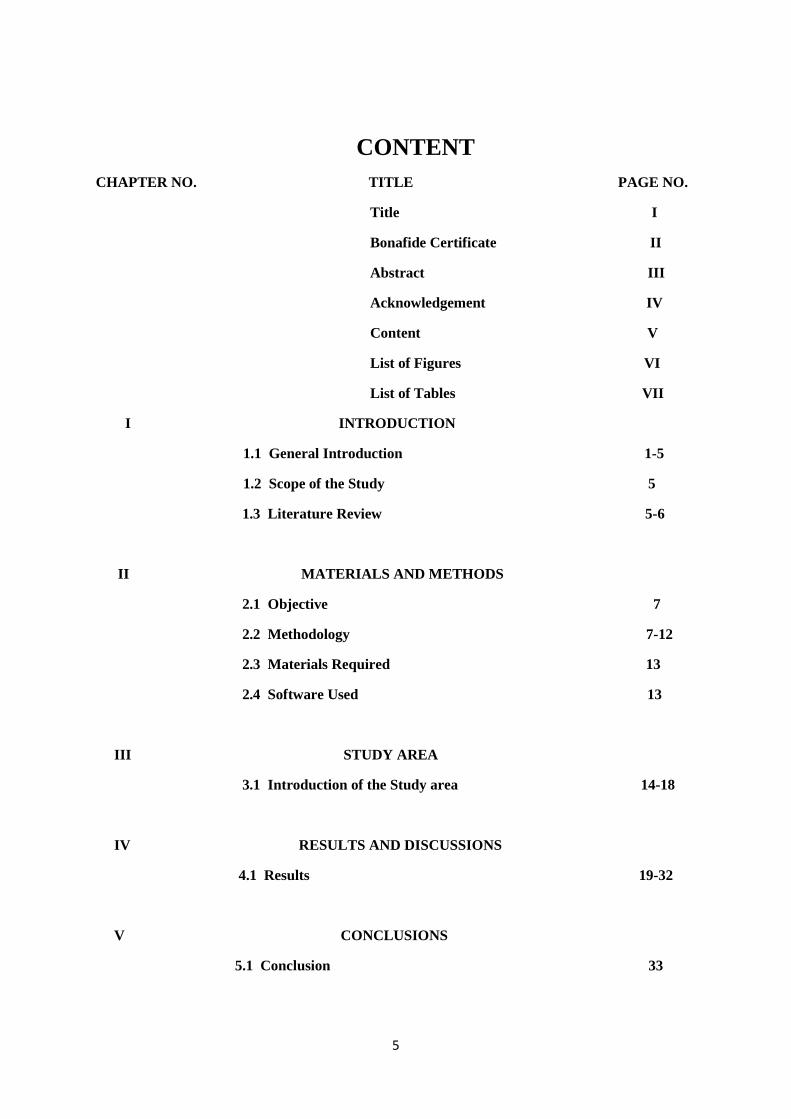
CONTENT CHAPTER NO. TITLE PAGE NO.
Title I
Bonafide Certificate II
Abstract III
Acknowledgement IV
Content V
List of Figures VI
List of Tables VII
I INTRODUCTION
1.1 General Introduction 1-5
1.2 Scope of the Study 5
1.3 Literature Review 5-6
II MATERIALS AND METHODS
2.1 Objective 7
2.2 Methodology 7-12
2.3 Materials Required 13
2.4 Software Used 13
III STUDY AREA
3.1 Introduction of the Study area 14-18
IV RESULTS AND DISCUSSIONS
4.1 Results 19-32
V CONCLUSIONS
5.1 Conclusion 33
6
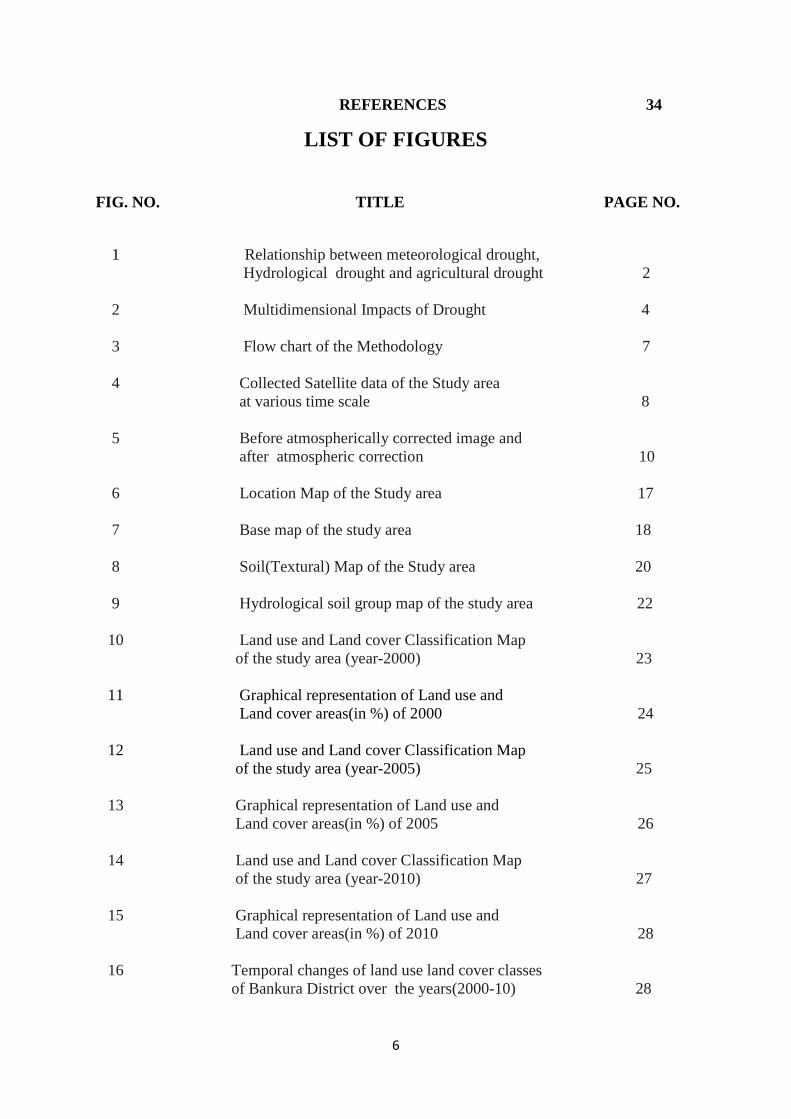
REFERENCES 34
LIST OF FIGURES
FIG. NO. TITLE PAGE NO.
1 Relationship between meteorological drought, Hydrological drought and agricultural drought 2 2 Multidimensional Impacts of Drought 4 3 Flow chart of the Methodology 7 4 Collected Satellite data of the Study area at various time scale 8 5 Before atmospherically corrected image and after atmospheric correction 10 6 Location Map of the Study area 17 7 Base map of the study area 18 8 Soil(Textural) Map of the Study area 20 9 Hydrological soil group map of the study area 22 10 Land use and Land cover Classification Map of the study area (year-2000) 23 11 Graphical representation of Land use and Land cover areas(in %) of 2000 24 12 Land use and Land cover Classification Map of the study area (year-2005) 25 13 Graphical representation of Land use and Land cover areas(in %) of 2005 26 14 Land use and Land cover Classification Map of the study area (year-2010) 27 15 Graphical representation of Land use and Land cover areas(in %) of 2010 28 16 Temporal changes of land use land cover classes of Bankura District over the years(2000-10) 28
7
LIST OF TABLES TABLE NO. TITLE PAGE NO.
1 Characteristics of Satellite Imageries used in this study 13 2 Different Classes of Hydrological Soil Group Contains respective soil type(Texture) 21 3 Net change (in %) of LULC areas of Bankura District from 2000 to 2010 29
8
CHAPTER I
INTRODUCTION
1.1 GENERAL INTRODUCTION
Drought may be defined as an extended period – a season, a year or more - of deficient
rainfall relative to the statistical multi-year average for a region. It is a normal and recurrent
feature of climate and may occur anywhere in the world, in all climatic zones. Its features or
characteristics, of course, vary from region to region.
Simply put, drought is a period of drier-than-normal conditions that lead to water
related problems. When rainfall is below normal for weeks, months or even years, it brings
about a decline in the flow of rivers and streams and a drop in water levels in reservoirs and
wells. If dry weather persists and water supply-related problems increase, the dry period can
be called a drought. Drought cannot be confined to a single all-encompassing definition. It
depends on differences in regions, needs and disciplinary perspectives.
1.1.1 Drought classification:
There are a number of classifications for drought. A permanent drought is
characterised by extremely dry climate, drought vegetation and agriculture that is possible
only by irrigation; seasonal drought requires crop durations to be synchronised with the rainy
season; contingent drought is of irregular occurrence; and invisible drought occurs even when
there is frequent rainfall, in humid regions (Thornthwaite-1947). Physical aspects are also
used to classify drought. They may be clubbed into three or Three major groups:
• Meteorological drought, is related to deficiencies in rainfall compared to the average
mean annual rainfall in an area. There is, however, no consensus on the threshold of
deficit that makes a dry spell an official drought. According to the India
Meteorological Department (IMD), meteorological drought occurs when the seasonal
rainfall received over an area is less than 75% of its long-term average value. If the
rainfall deficit is between 26-50%, the drought is classified as 'moderate', and 'severe'
if the deficit exceeds 50%.
.
9
• Hydrological drought, is a deficiency in surface and sub-surface water supply. It is
measured as stream flows and also as lake, reservoir and groundwater levels.
• Agricultural drought, occurs when there is insufficient soil moisture to meet the
needs of a particular crop at a particular point in time. Deficit rainfall over cropped
areas during their growth cycle can destroy crops or lead to poor crop yields.
Agricultural drought is typically witnessed after a meteorological drought, but before
a hydrological drought.
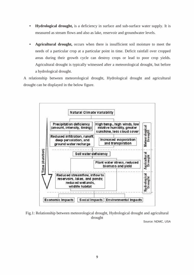
A relationship between meteorological drought, Hydrological drought and agricultural
drought can be displayed in the below figure.
Fig.1: Relationship between meteorological drought, Hydrological drought and agricultural drought
Source: NDMC, USA
10
1.1.2 Impacts of drought:
Drought has a direct and indirect impact on the economic, social and environmental
fabric of the country. Depending on its reach and scale it could bring about social unrest. The
Employment Guarantee Scheme (EGS) that the Maharashtra government put in place was a
direct outcome of the 1971-72 drought. The immediate visible impact of monsoon failure
leading to drought is felt by the agricultural sector. The impact passes on to other sectors,
including industry, through one or more of the following routes:
• A shortage of raw material supplies to agro-based industries.
• Reduced rural demand for industrial/consumer products due to reduced agricultural
incomes.
• Potential shift in public sector resource allocation from investment expenditure to
financing of drought relief measures.
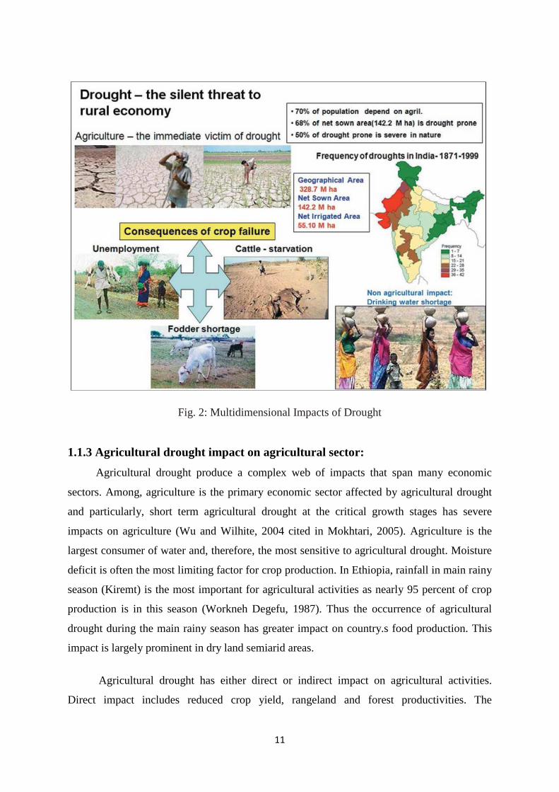
� Economic Impact: Many economic impacts occur in agriculture and related sectors, including forestry and fisheries, because of the reliance of these sectors on surface and subsurface water supplies. In addition to obvious losses in yields in crop and livestock production. Drought is associated with increases in insect infections, plant disease and wind erosion. The incidence of forest and range fires increases substantially during extended droughts, which in turn places both human and wildlife populations at higher levels of risk. � Environmental Impact: Environmental losses are the result of damages to plant and animal species, wildlife habitat and air and water qualiy; forest and range fires; degradation of landscapes; loss of biodiversity and soil erosion. Some of the effects are short term and conditions quickly return to normal following the end of the drought. Other environmental effects linger for some time or may even become permanent, wildlife habitat. For example, may be degraded through the loss of wetlands, lakes and vegetation. The degradation of landscape quality, including increased soil erosion may lead to a more permanent loss of biological productivity of the landscape. � Social Impact: Social impacts involve public safety, health, conflicts between water users, reduced quality of life and inequities in the distribution of impacts and disaster relief. Many of the impacts identified as economic and environmental have social components as well. Population migration is a significant problem in many countries, often stimulated by greater supply of food and water elsewhere. Migration is usually to urban areas within the stressed area or to regions outside the drought area. Migration may even be to adjacent countries. The drought migrants place increasing pressure on the social infrasttructure of the urban areas, leading to increased poverty and social unrest.
11
Fig. 2: Multidimensional Impacts of Drought
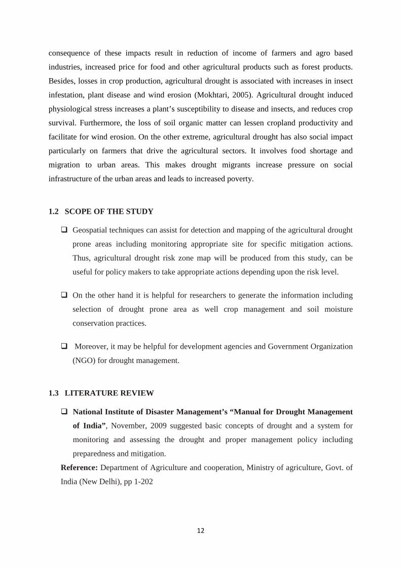
1.1.3 Agricultural drought impact on agricultural sector:
Agricultural drought produce a complex web of impacts that span many economic
sectors. Among, agriculture is the primary economic sector affected by agricultural drought
and particularly, short term agricultural drought at the critical growth stages has severe
impacts on agriculture (Wu and Wilhite, 2004 cited in Mokhtari, 2005). Agriculture is the
largest consumer of water and, therefore, the most sensitive to agricultural drought. Moisture
deficit is often the most limiting factor for crop production. In Ethiopia, rainfall in main rainy
season (Kiremt) is the most important for agricultural activities as nearly 95 percent of crop
production is in this season (Workneh Degefu, 1987). Thus the occurrence of agricultural
drought during the main rainy season has greater impact on country.s food production. This
impact is largely prominent in dry land semiarid areas.
Agricultural drought has either direct or indirect impact on agricultural activities.
Direct impact includes reduced crop yield, rangeland and forest productivities. The
12
consequence of these impacts result in reduction of income of farmers and agro based
industries, increased price for food and other agricultural products such as forest products.
Besides, losses in crop production, agricultural drought is associated with increases in insect
infestation, plant disease and wind erosion (Mokhtari, 2005). Agricultural drought induced
physiological stress increases a plant’s susceptibility to disease and insects, and reduces crop
survival. Furthermore, the loss of soil organic matter can lessen cropland productivity and
facilitate for wind erosion. On the other extreme, agricultural drought has also social impact
particularly on farmers that drive the agricultural sectors. It involves food shortage and
migration to urban areas. This makes drought migrants increase pressure on social
infrastructure of the urban areas and leads to increased poverty.
1.2 SCOPE OF THE STUDY
� Geospatial techniques can assist for detection and mapping of the agricultural drought
prone areas including monitoring appropriate site for specific mitigation actions.
Thus, agricultural drought risk zone map will be produced from this study, can be
useful for policy makers to take appropriate actions depending upon the risk level.
� On the other hand it is helpful for researchers to generate the information including
selection of drought prone area as well crop management and soil moisture
conservation practices.
� Moreover, it may be helpful for development agencies and Government Organization
(NGO) for drought management.
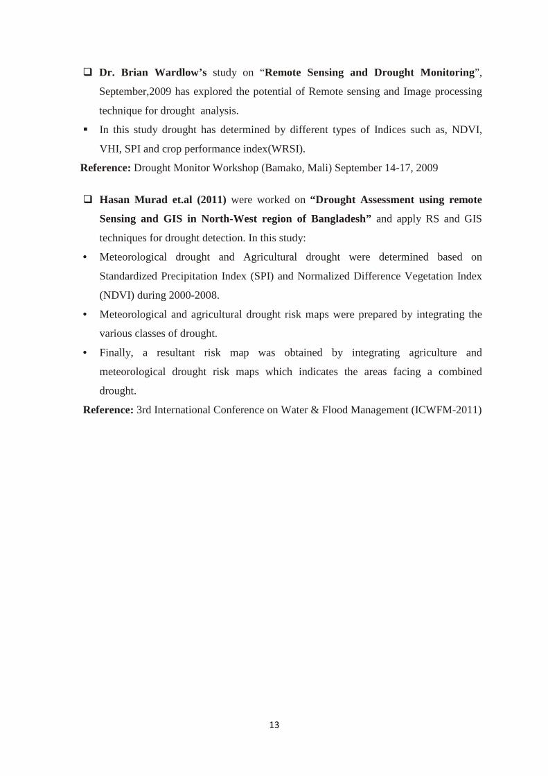
1.3 LITERATURE REVIEW
� National Institute of Disaster Management’s “Manual for Drought Management
of India” , November, 2009 suggested basic concepts of drought and a system for
monitoring and assessing the drought and proper management policy including
preparedness and mitigation.
Reference: Department of Agriculture and cooperation, Ministry of agriculture, Govt. of
India (New Delhi), pp 1-202
13
� Dr. Brian Wardlow’s study on “Remote Sensing and Drought Monitoring”,
September,2009 has explored the potential of Remote sensing and Image processing
technique for drought analysis.
� In this study drought has determined by different types of Indices such as, NDVI,
VHI, SPI and crop performance index(WRSI).
Reference: Drought Monitor Workshop (Bamako, Mali) September 14-17, 2009
� Hasan Murad et.al (2011) were worked on “Drought Assessment using remote
Sensing and GIS in North-West region of Bangladesh” and apply RS and GIS
techniques for drought detection. In this study:
• Meteorological drought and Agricultural drought were determined based on
Standardized Precipitation Index (SPI) and Normalized Difference Vegetation Index
(NDVI) during 2000-2008.
• Meteorological and agricultural drought risk maps were prepared by integrating the
various classes of drought.
• Finally, a resultant risk map was obtained by integrating agriculture and
meteorological drought risk maps which indicates the areas facing a combined
drought.
Reference: 3rd International Conference on Water & Flood Management (ICWFM-2011)
14
CHAPTER II
MATERIALS AND METHODS
2.1 OBJECTIVES The first and foremost objective of the study is to assess the spatiotemporal
occurrence of agricultural drought and their impacts on agricultural production.
For achieving the objective, the following analyses are required:
� Drought risk assessment using remotely sensed image based vegetation,
precipitation, Temperature and soil adjusted indices.
� Impact of drought on agriculture
� Drought risk zone map showing the severity of drought condition at various levels
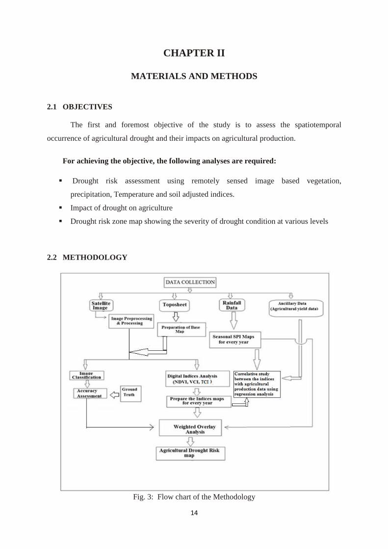
2.2 METHODOLOGY
Fig. 3: Flow chart of the Methodology
15
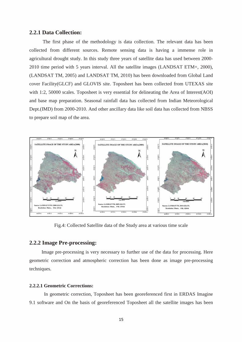
2.2.1 Data Collection:
The first phase of the methodology is data collection. The relevant data has been
collected from different sources. Remote sensing data is having a immense role in
agricultural drought study. In this study three years of satellite data has used between 2000-
2010 time period with 5 years interval. All the satellite images (LANDSAT ETM+, 2000),
(LANDSAT TM, 2005) and LANDSAT TM, 2010) has been downloaded from Global Land
cover Facility(GLCF) and GLOVIS site. Toposheet has been collected from UTEXAS site
with 1:2, 50000 scales. Toposheet is very essential for delineating the Area of Interest(AOI)
and base map preparation. Seasonal rainfall data has collected from Indian Meteorological
Dept.(IMD) from 2000-2010. And other ancillary data like soil data has collected from NBSS
to prepare soil map of the area.
Fig.4: Collected Satellite data of the Study area at various time scale 2.2.2 Image Pre-processing:
Image pre-processing is very necessary to further use of the data for processing. Here
geometric correction and atmospheric correction has been done as image pre-processing
techniques.
2.2.2.1 Geometric Corrections:
In geometric correction, Toposheet has been georeferenced first in ERDAS Imagine
9.1 software and On the basis of georeferenced Toposheet all the satellite images has been

16
georeferenced by using Image to Image georeferencing technique in Erdas Imagine 9.1
software one by one.
2.2.2.2 Atmospheric Corrections:
However, there is no commonly accepted correction for Landsat data for operational
applications at regional scale. Here atmospheric correction model was adapted from
"Atmospheric and radiometric correction of Landsat TM 5 Data using the COST model
(Chavez, 1996", S. M. Skirvin).
The inputs to the COST model are the Earth-Sun Distance, sun elevation angle, and
minimum DN values for each band. The model first converts each minimum DN value to
minimum spectral radiance value:
Lλ������ = LMINλ + QCAL ∗ (LMAXλ − LMINλ)/QCALMAX ............................. Eq. 1
Lλsensor =apparent at-satellite radiance, LMAXλ =the spectral radiance that is scaled to
QCALMIN in watts/(meter squared * ster * µm), LMAXλ=the spectral radiance that is scaled
to QCALMAX in watts/(meter squared * ster * µm),QCAL= the quantized calibrated pixel
value in DN, QCALMAX=the minimum quantized calibrated pixel value(corresponding to
LMIN λ) in DN. The value of QCALMAX,QCALMIN,LMAXλand LMAXλ values can be
obtained from the Metadata file of the respective image. For each band, the theoretical
radiance of a dark object (assumed to have a reflectance of 1% by Chavez 1996 and Moran et
al. 1992) is computed:
Lλ,�% = .01 ∗ d�cos�θ/(π ∗ ESUNλ) ............................................. Eq. 2
Where, ESUNλ=mean solar exatmosperic spectral radiance from Table 4 of Markham and
Barker (1986), d is the sun-earth distance can be obtained from http://ssd.jpl.nasa.gov/cgi-
bin/eph, and theta(θ) is the solar zenith angle (90-sun elev).The value of sun elevation angle
can be found in Metadata of the image. A haze correction is computed using the computed
dark object values (Chavez 1996):
Lλ,&'(� = Lλ������ − Lλ,�% ..................................................... Eq. 3
The fundamental radiance to surface reflectance (rho) equation ( Chavez 1996) is:
ρ = π ∗ d�(L������ − Lλ,&'(�)/ESUNλ ∗ COS�θ ........................................................ Eq. 4
The output from the model is in reflectance units, which should range from 0 to 1.
Occasionally, values greater than 1 are obtained, and these generally correspond to bright
objects (e.g., clouds, snow, playa) or sometimes noise (randomly or systematically scattered
saturated pixels). The Landsat 5 Atmospheric and Radiometric Correction output data format
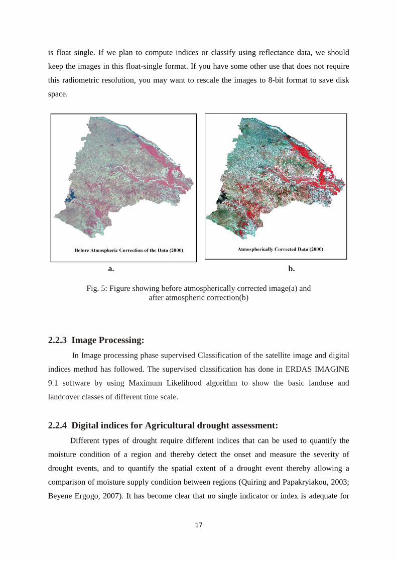
17
is float single. If we plan to compute indices or classify using reflectance data, we should
keep the images in this float-single format. If you have some other use that does not require
this radiometric resolution, you may want to rescale the images to 8-bit format to save disk
space.
a. b.
Fig. 5: Figure showing before atmospherically corrected image(a) and
after atmospheric correction(b)
2.2.3 Image Processing:
In Image processing phase supervised Classification of the satellite image and digital
indices method has followed. The supervised classification has done in ERDAS IMAGINE
9.1 software by using Maximum Likelihood algorithm to show the basic landuse and
landcover classes of different time scale.
2.2.4 Digital indices for Agricultural drought assessment:
Different types of drought require different indices that can be used to quantify the
moisture condition of a region and thereby detect the onset and measure the severity of
drought events, and to quantify the spatial extent of a drought event thereby allowing a
comparison of moisture supply condition between regions (Quiring and Papakryiakou, 2003;
Beyene Ergogo, 2007). It has become clear that no single indicator or index is adequate for
18
monitoring drought on regional scale. Instead, a combination of monitoring tools integrated
together is preferable for producing regional or national maps (Martini et al., 2004). Thus,
spatiotemporal patterns of seasonal drought can be detected using meteorological, vegetative
as well as crop performance indices among others.
2.2.4.1 Normalized Difference vegetation Index:
NDVI is an index of vegetation health and density and computed from the satellite Image
using spectral radiance in red and near infrared reflectance using the formula:
NDVI= (NIR-R) / (NIR+R); Where NIR= near infrared band, R= Red band
NDVI is a powerful indicator to monitor the vegetation cover of wide areas, and to detect the
frequent occurrence and persistence of droughts (Thavorntam and Mongkolsawat, 2006). It
provides a measure of the amount and vigor of vegetation at the land surface. The magnitude
of NDVI is related to the level of photosynthetic activity in the observed vegetation. In
general, higher values of NDVI indicate greater vigor and amounts of vegetation. Tucker first
suggested NDVI in 1979 as an index of vegetation health and density (Thenkabail et al.,
2004) and it has been considered as the most important index for mapping of agricultural
drought (Vogt, 2000 cited in Mokhtari, 2005).
NDVI is a nonlinear function that varies between -1 and +1 and values of NDVI for
vegetated land generally range from about 0.1 to 0.7, with values greater than 0.5 indicating
dense vegetation (FEWSnet). NDVI is good indicator of green biomass, leaf area index and
patterns of production (Thenkabail et al., 2004). Furthermore, NDVI can be used not only for
accurate description of vegetation vigor, vegetation classification and continental land cover
but is also effective for monitoring rainfall and drought, estimating net primary production of
vegetation, crop growth conditions and crop yields, detecting weather impacts and other
events important for agriculture, ecology and economics (Ramesh et al., 2003).
2.2.4.2 Vegetation Condition Index:
Kogan (1990) developed Vegetation Condition Index (VCI) using the range of NDVI which
is a good indicator for assessing the severity of agricultural drought.
VCI = (NDVI-NDVI min) / (NDVI max-NDVI min)*100
19
Where, NDVI is the actual value of NDVI , NDVI max and NDVI min are smoothed weekly
NDVI absolute maximum and its minimum.
The VCI values between 50 to 100 % indicate optimal or above-normal conditions.
At the VCI value of 100% the NDVI value for this month (or week) is equal to NDVImax.
Different degrees of a drought severity are indicated by VCI values below 50%.
2.2.4.3 Temperature Condition Index:
TCI is also suggested by Kogan(1997). It was developed to reflect vegetation response to
temperature i.e. higher the temperature more extreme the drought. TCI is besed on brightness
temperature and represents the deviation of current month’s value from the recorded
maximum. It is defined as:
TCI = (BT max-BT) / (BT max-BT min)*100
Where, BT, BT max and BT min are smoothed weekly brightness
temperature absolute maximum and its minimum.
The TCI value of 50 % indicates the normal condition or no drought. At the TCI
value of 100% represents the optimal/above normal condition and Different degrees of a
drought severity are indicated by TCI values below 50%.
2.2.4.4 Standardized Precipitation Index:
Standardized Precipitation Index (SPI) is an index that was developed to quantify
precipitation deficit at different time scales, and can also help assess drought severity. It is
defined as:
SPI = {(Xij − Xim) /ó }
where, (Xij= is the seasonal precipitation and, Xim is its long-term seasonal mean and ó is it’s
standard deviation.)
20
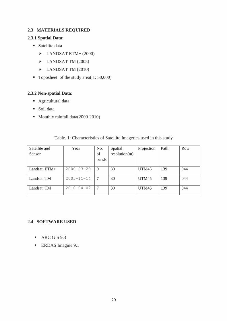
2.3 MATERIALS REQUIRED
2.3.1 Spatial Data:
� Satellite data
� LANDSAT ETM+ (2000)
� LANDSAT TM (2005)
� LANDSAT TM (2010)
� Toposheet of the study area( 1: 50,000)
2.3.2 Non-spatial Data:
� Agricultural data
� Soil data
� Monthly rainfall data(2000-2010)
Table. 1: Characteristics of Satellite Imageries used in this study
Satellite and Sensor
Year No. of bands
Spatial resolution(m)
Projection Path Row
Landsat ETM+ 2000-03-29 9 30 UTM45 139 044
Landsat TM 2005-11-14 7 30 UTM45 139 044
Landsat TM 2010-04-02 7 30 UTM45 139 044
2.4 SOFTWARE USED
� ARC GIS 9.3
� ERDAS Imagine 9.1
21
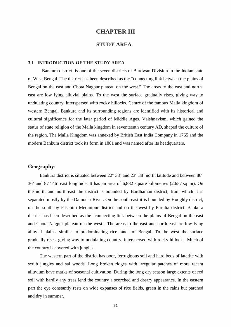
CHAPTER III STUDY AREA
3.1 INTRODUCTION OF THE STUDY AREA
Bankura district is one of the seven districts of Burdwan Division in the Indian state
of West Bengal. The district has been described as the “connecting link between the plains of
Bengal on the east and Chota Nagpur plateau on the west.” The areas to the east and north-
east are low lying alluvial plains. To the west the surface gradually rises, giving way to
undulating country, interspersed with rocky hillocks. Centre of the famous Malla kingdom of
western Bengal, Bankura and its surrounding regions are identified with its historical and
cultural significance for the later period of Middle Ages. Vaishnavism, which gained the
status of state religion of the Malla kingdom in seventeenth century AD, shaped the culture of
the region. The Malla Kingdom was annexed by British East India Company in 1765 and the
modern Bankura district took its form in 1881 and was named after its headquarters.
Geography:
Bankura district is situated between 22° 38’ and 23° 38’ north latitude and between 86°
36’ and 87° 46’ east longitude. It has an area of 6,882 square kilometres (2,657 sq mi). On
the north and north-east the district is bounded by Bardhaman district, from which it is
separated mostly by the Damodar River. On the south-east it is bounded by Hooghly district,
on the south by Paschim Medinipur district and on the west by Purulia district. Bankura
district has been described as the “connecting link between the plains of Bengal on the east
and Chota Nagpur plateau on the west.” The areas to the east and north-east are low lying
alluvial plains, similar to predominating rice lands of Bengal. To the west the surface
gradually rises, giving way to undulating country, interspersed with rocky hillocks. Much of
the country is covered with jungles.
The western part of the district has poor, ferruginous soil and hard beds of laterite with
scrub jungles and sal woods. Long broken ridges with irregular patches of more recent
alluvium have marks of seasonal cultivation. During the long dry season large extents of red
soil with hardly any trees lend the country a scorched and dreary appearance. In the eastern
part the eye constantly rests on wide expanses of rice fields, green in the rains but parched
and dry in summer.
22
The Gondwana system is represented in the northern portion of the district, south of the
Damodar, between Mejia and Biharinath Hill. The beds covered with alluvium contains
seams of coal belonging to the Raniganj system.
Hills and River System:
The hills of the district consist of outliers of the Chota Nagpur plateau and only two are
of any great height – Biharinath and Susunia. While the former rises to a height of 448 metres
(1,470 ft), the latter attains a height of 440 metres (1,440 ft).
The rivers of the area flow from the north-east to the south-west in courses roughly
parallel to one another. They are mostly hill streams, originating in the hills in the west. The
rivers come down in floods after heavy rains and subside as rapidly as they rise. In summer,
their sand beds are almost always dry. The principal rivers are: Damodar, Dwarakeswar,
Shilabati, Kangsabati, Sali, Gandheswari, Kukhra, Birai, Jaypanda and Bhairabbanki. There
are some small but picturesque water falls along the course of the Shilabati near Harmasra,
and along the course of the Kangsabati in the Raipur area.
Kangsabati Project was started during the second five year plan period (1956–1961).
The dam across the Kangsabati has a length of 10,098 metres (33,130 ft) and a height of 38
metres (125 ft).
Climate:
The climate, especially in the upland tracts to the west, is much drier than in eastern or
southern Bengal. From the beginning of March to early June, hot westerly winds prevail, the
thermometer in the shade rising to around 45 °C (113 °F). The monsoon months, June to
September, are comparatively pleasant. The total average rainfall is 1,400 millimetres (55 in),
the bulk of the rain coming in the months of June to September. Winters are pleasant with
temperatures dropping down to below 27 °C (81 °F) in December.
Soil:
According to soil texture, 60207 hec. is Clay area, 81944 hec. is Loamy-Clay area and
the rest part is described as Sandy-Clay area.
23
Flora:
The eastern portion of the district forms part of the rice plains of West Bengal. The
land under rice cultivation contains the usual marsh weeds of Gangetic plain. Aquatic plants
and water weeds are found in ponds, ditches and still streams. Around human habitations
there are shrub species such as Glycosmis, Polyalthia suberosa, Clerodenaron infortunatum,
Solanum torvum, and various other species of the same genus, besides Trema, Streblus and
Ficus hispida. The larger trees are papal, banyan, red cotton tree (Bombax malabaricum),
mango (Mangifera indica), jiyal (Odina Wodier), Phoenix dactylifera, and Borassus
flabellifer. Other plants found include Jatropha gossypifolia, Urena, Heliotropium and Sida.
Forests or scrub jungles contain Wendlandia exserta, Gmelina arborea, Adina Cordifolia,
Holarrhena antidysenterica, Wrightia tomentosa, Vitex negundo and Stephegyne parvifolia.
The western portion of the district is higher. The uplands either bare or are covered
with scrub jungle of Zizyphus and other thorny shrubs. This thorny forest gradually merges
into sal (Shorea robusta) forest. Low hills are covered with Miliusa, Schleichera, Diospyros
and other trees.
Some of the common trees of economic interest found in the district are: Alkushi
(Mucuna pruriens), amaltas (Cassia Fistula), asan (Terminaliat omentosa), babul (Acacia
Arabica), bair (Zizyphus Jujuba), bael (Aegle Marmelos), bag bherenda (Jatropha curcas),
bichuti (Tragia involucrate), bahera (Terminalia belerica), dhatura (Datura stramonium),
dhaman (Cordia Macleoidii), gab (Diospyros Embyopteris), harra (Terminalia chebula), imli
(Tamarindus indica), kuchila (Strychnos Nux vomica), mahua (Bassia latifolia), palas (Butea
frondosa), sajina (Moringa pterygosperma), kend (Diospyros melanoxylon), mango, date-
palm, nim, papal, banyan, red cotton tree and jiyal.
24
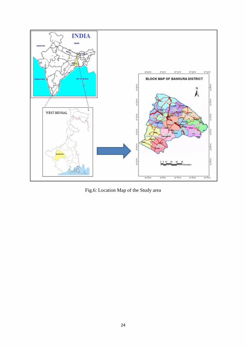
Fig.6: Location Map of the Study area
25
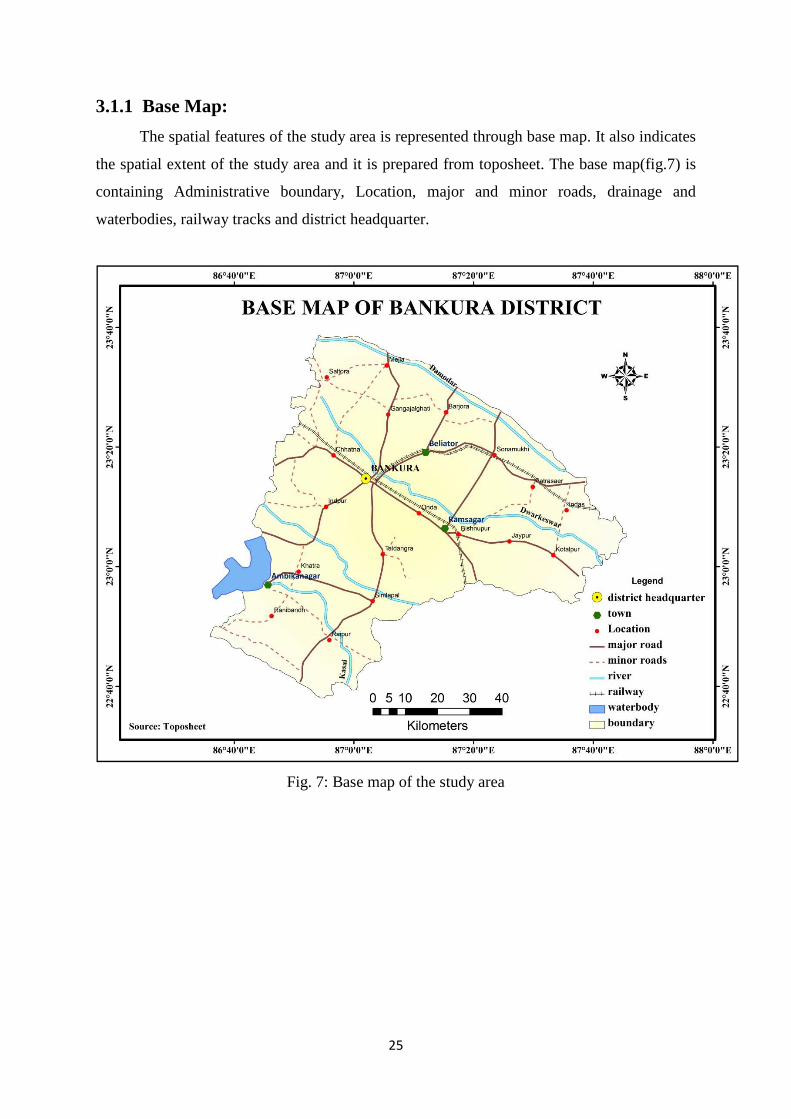
3.1.1 Base Map:
The spatial features of the study area is represented through base map. It also indicates
the spatial extent of the study area and it is prepared from toposheet. The base map(fig.7) is
containing Administrative boundary, Location, major and minor roads, drainage and
waterbodies, railway tracks and district headquarter.
Fig. 7: Base map of the study area
26
CHAPTER IV
RESULTS AND DISCUSSION
4.1 RESULTS
The following results are obtained at the end of phase-I project. The work has performed
basically preparation soil type map and hydrological soil group map through digitization and
database generation in ARC GIS 9.3 software and the supervised classification of the
temporal images and identified the basic landuse and landcover types and patterns over the
study area and also NDVI has performed to determine the vegetation condition and
healthiness over the area in ERDAS Imagine 9.1 software.
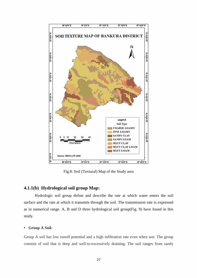
4.1.1(a) Soil(texture) Map:
The soil map (Fig. 8) of Bankura District represents the general soil type(textural) over
the entire area. These are mainly Coarse Loamy, Fine Loamy, Sandy Loam, Sandy Clay,
Silty Clay, Silty Loam and Silty Clay Loam. The soil attribute data has collected from NBSS,
LUP and the soil map is prepared.
27
Fig.8: Soil (Textural) Map of the Study area
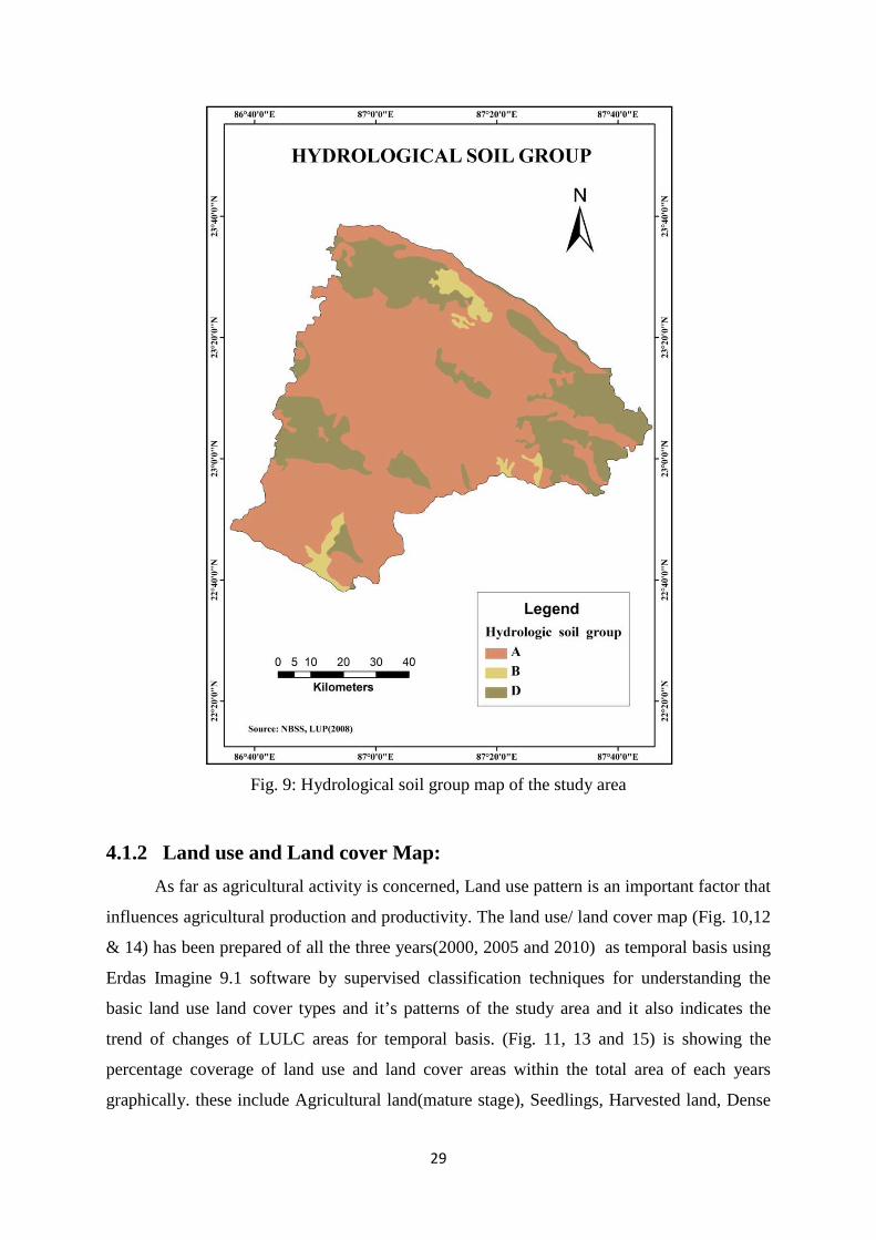
4.1.1(b) Hydrological soil group Map:
Hydrologic soil group define and describe the rate at which water enters the soil
surface and the rate at which it transmits through the soil. The transmission rate is expressed
as in numerical range. A, B and D three hydrological soil group(Fig. 9) have found in this
study.
• Group A Soil:
Group A soil has low runoff potential and a high infiltration rate even when wet. The group
consists of soil that is deep and well-to-excessively draining. The soil ranges from sandy
28
loam to high gravel content. The water transmission rate is greater than 0.30 inch per hour.
Sandy loam, coarse and fine loamy soil falls in this hydrologic soil group .
• Group B Soil:
Group B hydrologic soil classification indicates silt loam or loam soil. It has moderately fine-
to-moderately course texture created by its mineral particle content relative to its organic
matter content. It has small amounts of sand and clay in silt-size particles. It has moderate
water infiltration rates 0.15 to 0.30 inch per hour. They are moderately well draining soils.
• Group D Soil:
Hydrologic soil classification Group D consists of soils with high clay content and very low
rate of water transmission. The rate of water infiltration and transmission is 0 to 0.05 inch per
hour. Clay loam, silty clay loam, sandy clay, silty clay soil falls in this group.
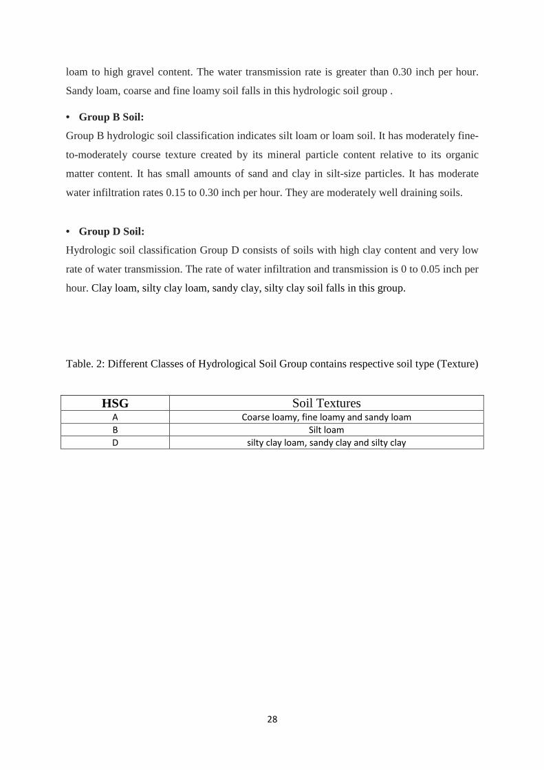
Table. 2: Different Classes of Hydrological Soil Group contains respective soil type (Texture)
HSG Soil Textures A Coarse loamy, fine loamy and sandy loam
B Silt loam
D silty clay loam, sandy clay and silty clay
29
Fig. 9: Hydrological soil group map of the study area
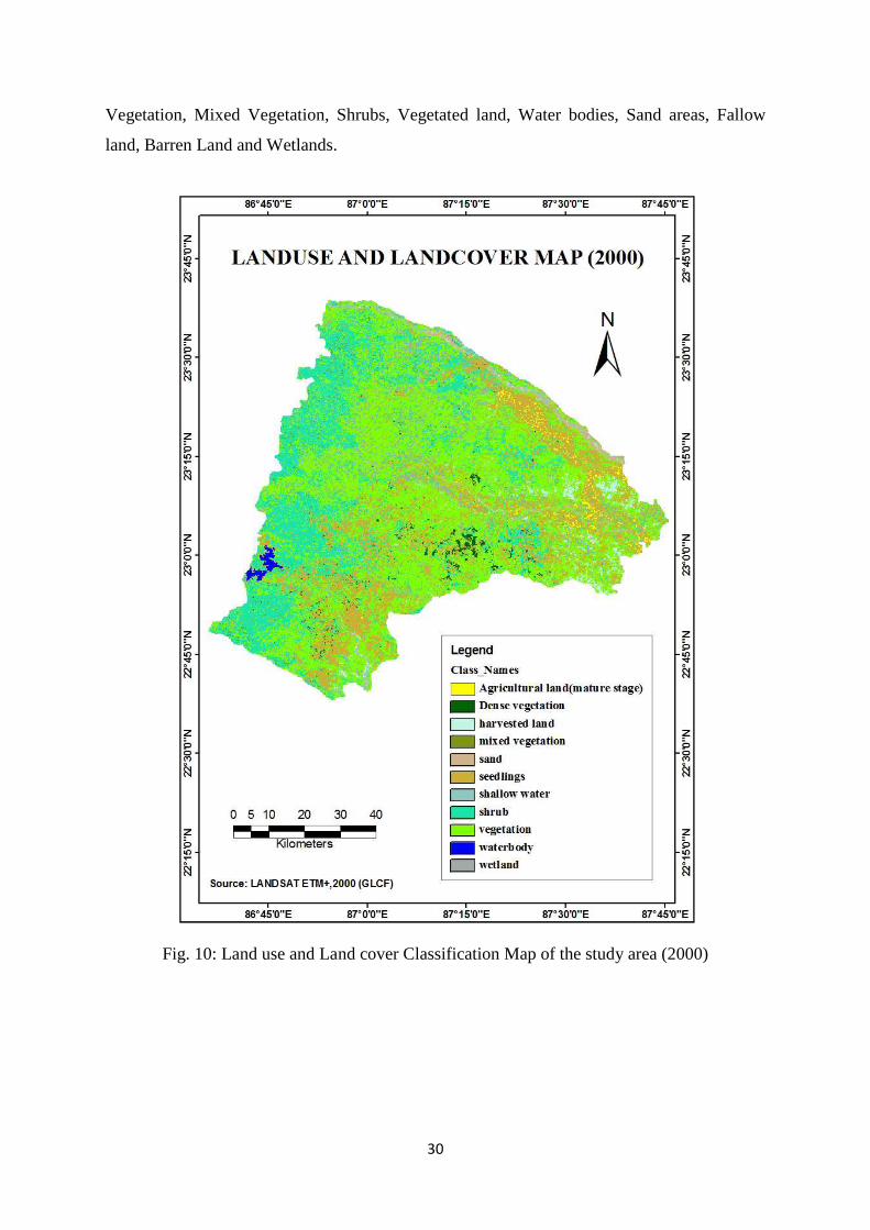
4.1.2 Land use and Land cover Map:
As far as agricultural activity is concerned, Land use pattern is an important factor that
influences agricultural production and productivity. The land use/ land cover map (Fig. 10,12
& 14) has been prepared of all the three years(2000, 2005 and 2010) as temporal basis using
Erdas Imagine 9.1 software by supervised classification techniques for understanding the
basic land use land cover types and it’s patterns of the study area and it also indicates the
trend of changes of LULC areas for temporal basis. (Fig. 11, 13 and 15) is showing the
percentage coverage of land use and land cover areas within the total area of each years
graphically. these include Agricultural land(mature stage), Seedlings, Harvested land, Dense
30
Vegetation, Mixed Vegetation, Shrubs, Vegetated land, Water bodies, Sand areas, Fallow
land, Barren Land and Wetlands.
Fig. 10: Land use and Land cover Classification Map of the study area (2000)
31
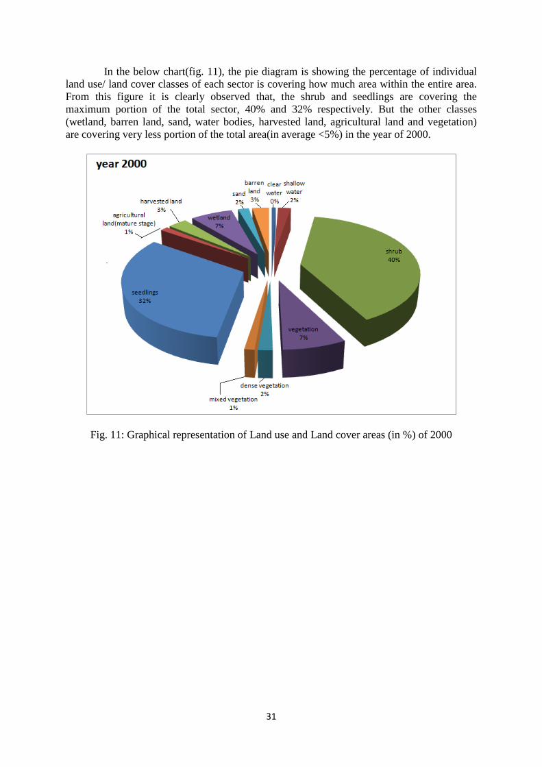
In the below chart(fig. 11), the pie diagram is showing the percentage of individual land use/ land cover classes of each sector is covering how much area within the entire area. From this figure it is clearly observed that, the shrub and seedlings are covering the maximum portion of the total sector, 40% and 32% respectively. But the other classes (wetland, barren land, sand, water bodies, harvested land, agricultural land and vegetation) are covering very less portion of the total area(in average <5%) in the year of 2000.
Fig. 11: Graphical representation of Land use and Land cover areas (in %) of 2000
32
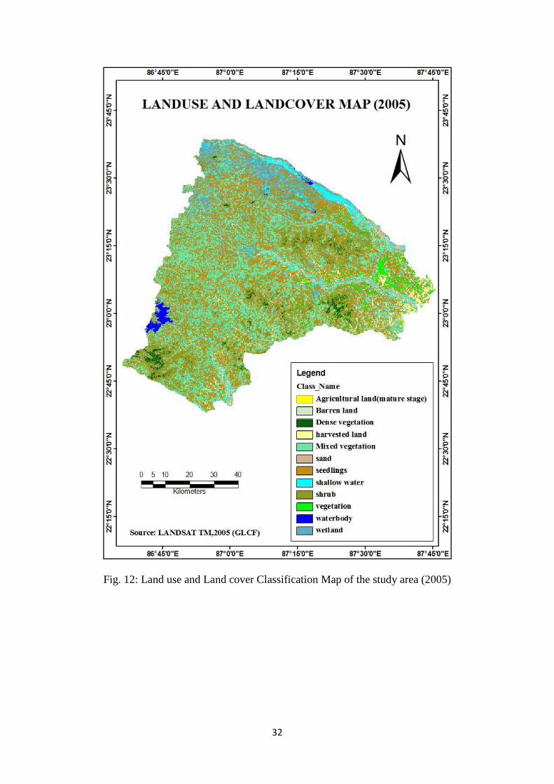
Fig. 12: Land use and Land cover Classification Map of the study area (2005)
33
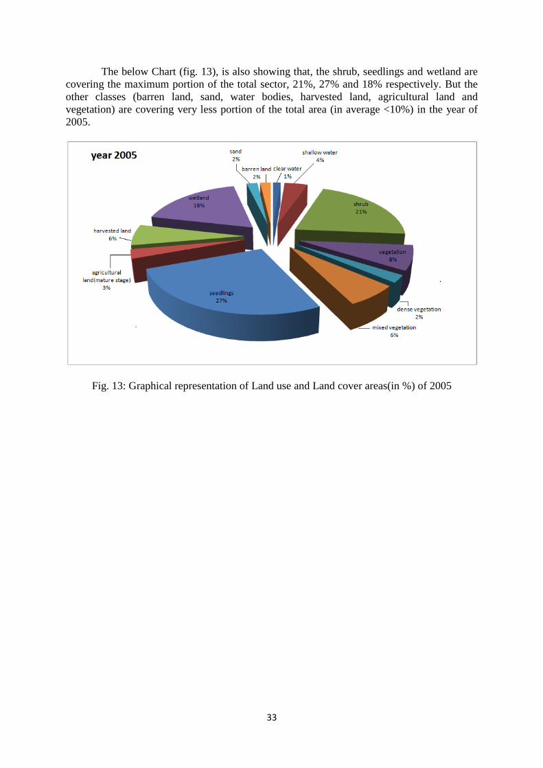
The below Chart (fig. 13), is also showing that, the shrub, seedlings and wetland are covering the maximum portion of the total sector, 21%, 27% and 18% respectively. But the other classes (barren land, sand, water bodies, harvested land, agricultural land and vegetation) are covering very less portion of the total area (in average <10%) in the year of 2005.
Fig. 13: Graphical representation of Land use and Land cover areas(in %) of 2005
34
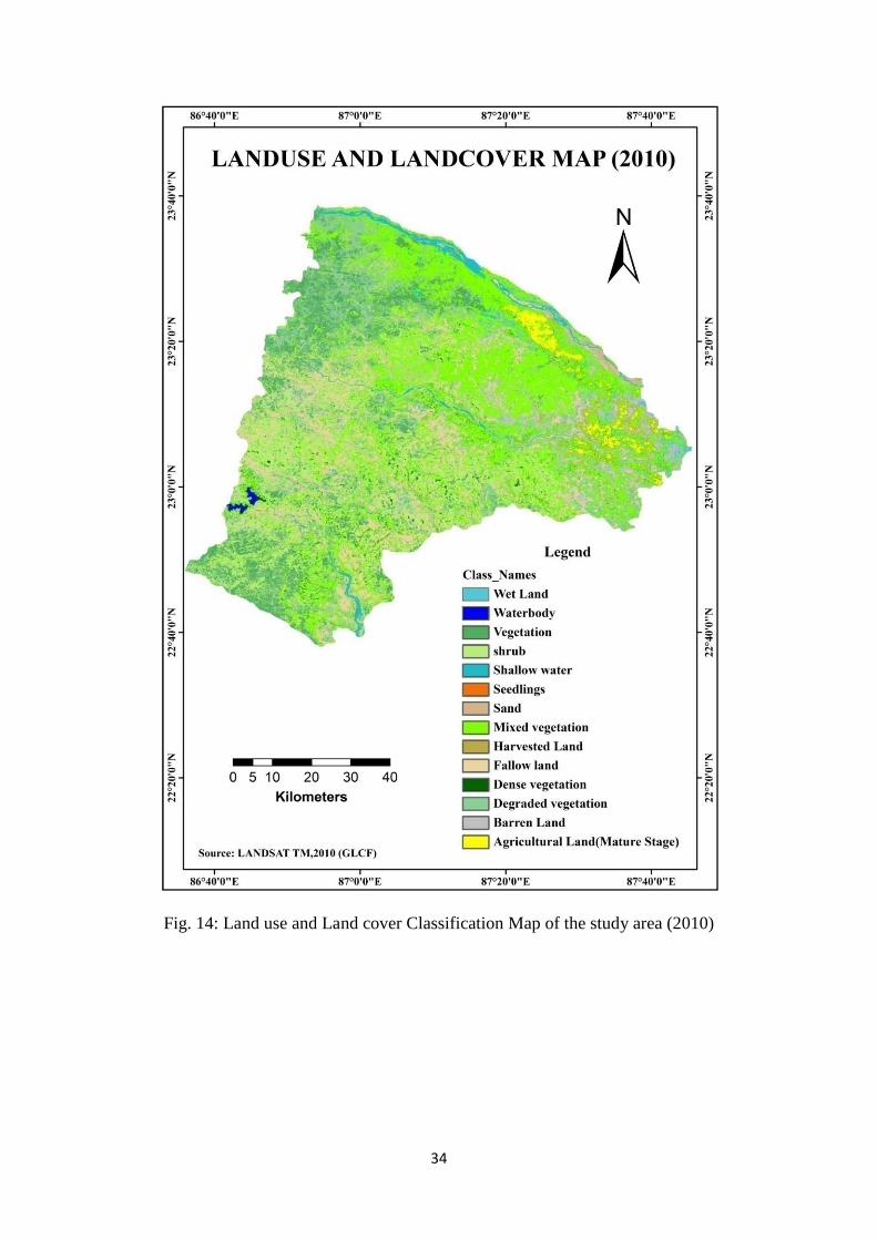
Fig. 14: Land use and Land cover Classification Map of the study area (2010)
35
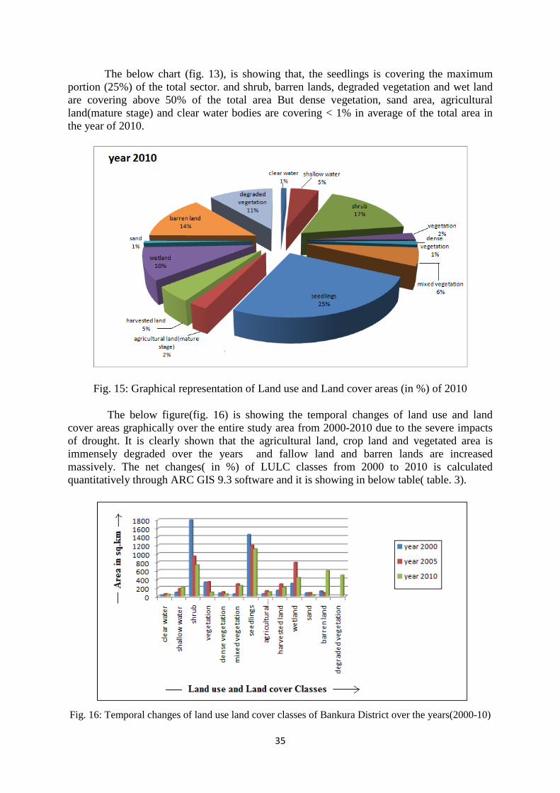
The below chart (fig. 13), is showing that, the seedlings is covering the maximum portion (25%) of the total sector. and shrub, barren lands, degraded vegetation and wet land are covering above 50% of the total area But dense vegetation, sand area, agricultural land(mature stage) and clear water bodies are covering < 1% in average of the total area in the year of 2010.
Fig. 15: Graphical representation of Land use and Land cover areas (in %) of 2010
The below figure(fig. 16) is showing the temporal changes of land use and land cover areas graphically over the entire study area from 2000-2010 due to the severe impacts of drought. It is clearly shown that the agricultural land, crop land and vegetated area is immensely degraded over the years and fallow land and barren lands are increased massively. The net changes( in %) of LULC classes from 2000 to 2010 is calculated quantitatively through ARC GIS 9.3 software and it is showing in below table( table. 3).
Fig. 16: Temporal changes of land use land cover classes of Bankura District over the years(2000-10)
36
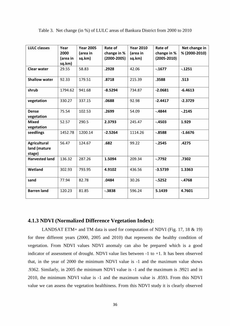
Table 3. Net change (in %) of LULC areas of Bankura District from 2000 to 2010
LULC classes Year
2000
(area in
sq.km)
Year 2005
(area in
sq.km)
Rate of
change in %
(2000-2005)
Year 2010
(area in
sq.km)
Rate of
change in %
(2005-2010)
Net change in
% (2000-2010)
Clear water 29.55
58.83
.2928 42.06
-.1677 -.1251
Shallow water 92.33
179.51
.8718 215.39
.3588 .513
shrub 1794.62
941.68
-8.5294 734.87
-2.0681 -6.4613
vegetation 330.27
337.15
.0688 92.98
-2.4417 -2.3729
Dense
vegetation
75.54
102.53
.2699 54.09
-.4844 -.2145
Mixed
vegetation
52.57
290.5
2.3793 245.47
-.4503 1.929
seedlings 1452.78
1200.14
-2.5264 1114.26
-.8588 -1.6676
Agricultural
land (mature
stage)
56.47
124.67
.682 99.22
-.2545 .4275
Harvested land 136.32
287.26
1.5094 209.34
-.7792 .7302
Wetland 302.93
793.95
4.9102 436.56
-3.5739 1.3363
sand 77.94
82.78
.0484 30.26
-.5252 -.4768
Barren land 120.23
81.85
-.3838 596.24
5.1439 4.7601
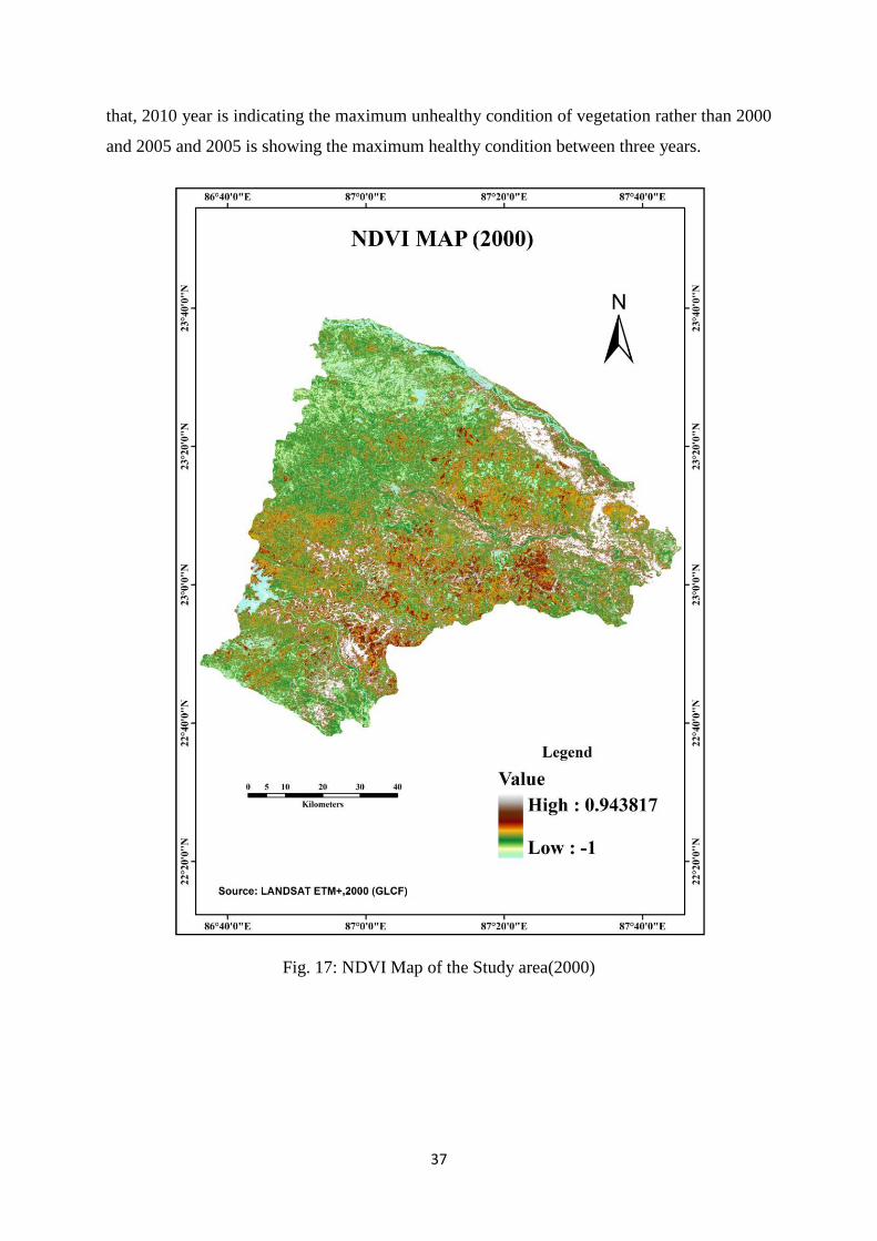
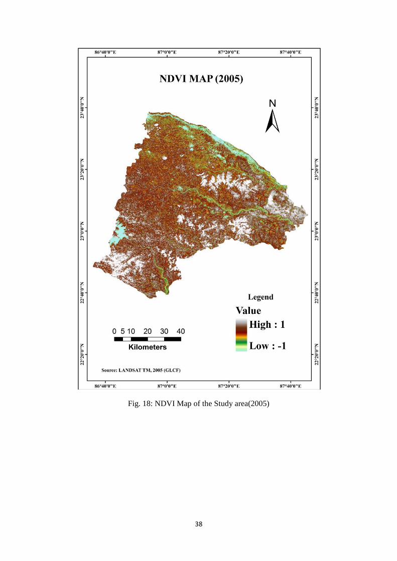
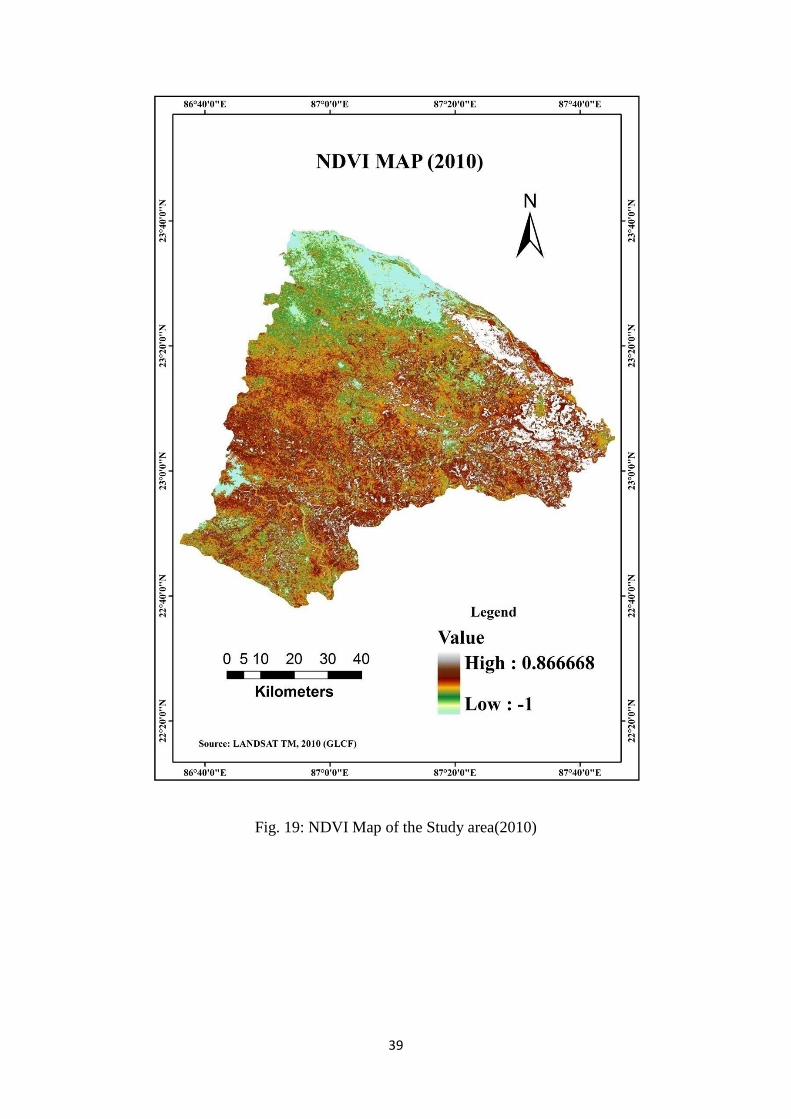
4.1.3 NDVI (Normalized Difference Vegetation Index):
LANDSAT ETM+ and TM data is used for computation of NDVI (Fig. 17, 18 & 19)
for three different years (2000, 2005 and 2010) that represents the healthy condition of
vegetation. From NDVI values NDVI anomaly can also be prepared which is a good
indicator of assessment of drought. NDVI value lies between -1 to +1. It has been observed
that, in the year of 2000 the minimum NDVI value is -1 and the maximum value shows
.9362. Similarly, in 2005 the minimum NDVI value is -1 and the maximum is .9921 and in
2010, the minimum NDVI value is -1 and the maximum value is .8593. From this NDVI
value we can assess the vegetation healthiness. From this NDVI study it is clearly observed
37
that, 2010 year is indicating the maximum unhealthy condition of vegetation rather than 2000
and 2005 and 2005 is showing the maximum healthy condition between three years.
Fig. 17: NDVI Map of the Study area(2000)
38
Fig. 18: NDVI Map of the Study area(2005)
39
Fig. 19: NDVI Map of the Study area(2010)
40
CHAPTER V CONCLUSION 5.1 CONCLUSION
The major work carried out in the phase- I project is the data collection for agricultural
drought assessment over the entire Bankura District, West Bengal along with that the
preparation of objective and methodology for reaching to the tentative conclusion by using
Optimal GIS and Remote Sensing techniques. Thus in major findings soil, base map were
prepared along with that indices based approach to analyze the spatio - temporal scenario
over the study area due to drought, classification were adopted to separate land use/land
cover classes and to view the area conversion because of drought over the study area from the
year 2000 to 2010. The base map showing spatial features such as roads, railways with
administrative boundary and geographical areas and location provide the vision about the
study area. Soil map showing the variation in the soil strata and textural components over the
area with different types and characterization on the basis of texture and structure and soil
hydrological group. The Land use/ Land cover maps over the years showing the basic LULC
types , patterns and temporal variation over the years due to the impact of drought and NDVI
maps are showing the vegetation conditions and healthiness and variation due to the severity
of drought and Remote Sensing and GIS is the best tool to temporally and quantitatively
analyze the drought severity over the agriculture and assessment.
41
REFERENCES
♣ Anyamba, A. and Tucker, C.J. (2005). Analysis of Sahelian vegetation dynamics
using NOAA-AVHRR NDVI data from 1981-2003. Journal of Arid Environment,
63:596.614.
♣ Aslam, M., Khan, I., M., Saleem, A. and Ali, Z. (2006). Assessment of water stress
tolerance in different maize accessions at germination and early growth stage.
Pakistan Journal of Botany, 38: 1571- 1579
♣ Bastiaanssen, 1998, Remote Sensing in Water Resources Management: The state of
the art, IWMI publication, p118.
♣ Batista TT, Shimabukuro YE and Lawrence WT, 1997, The long term monitoring of
vegetation cover in the Amazonian region of northern Brazil using NOAA-AVHRR
data, International Journal of Remote Sensing, 18: 3195-3210.
♣ Chopra, P. (2006). Drought risk assessment using remote sensing and GIS: A case
study of Gujarat. Msc. Thesis, ITC, Enschede.
♣ Comenetz, J. and Caviedes, C. (2002). Climate variability, political crises, and
historical population displacements in Ethiopia. Environmental Hazards, 4: 113-127.
♣ Dracup, J. A., Lee, K. S. and Paulson, E. G. (1980). On the definition of droughts.
Water Resources Research, 16:297-302
♣ Goldberg I, Ed., 1972, Agro climatic atlas of the World, Hydrometizdat, p 133
♣ Jeyaseelan, A.T. (2004). Drought and flood assessment and monitoring using remote
sensing and GIS.URL: http://www.wamis.org/agm/pubs/agm8/Paper-14.pdf
♣ Kogan,F.N. (1997). Contribution of Remote Sensing to Drought Early Warning.
42
♣ URL: http://drought.unl.edu/monitor/EWS/ch7_Kogan.pdf
♣ Ball, M.C. 1998. Mangrove species richness in relation to salinity and water logging. Global Ecology and Biogeography Letters7:73-82.
♣ Banerjee, L.K., A.R.K. Sastry & M.P. Nayar. 1989. Mangroves in India, Identification Manual. Botanical Survey of India, Kolkata.
♣ B. Meza D´ıaz and G. A. Blackburn Remote sensing of mangrove biophysical properties: evidence from a laboratory simulation of the possible effects of background variation on spectral vegetation indices, INT.J.Remote Sensing, 2003,vol 24, No 1, 53 - 73
♣ Chen, R. & R.R. Twilley. 1998. A gap dynamic model of mangrove forest development along gradients of soil salinity and nutrient resources. Journal of Ecology 86: 37-52.
♣ Chen, R. & R.R. Twilley. 1999. Patterns of mangrove forest structure and soil nutrient dynamics along the Shark River estuary, Florida. Estuaries 22: 955-970.
♣ Jordan, C. F., 1969, Derivation of leaf area index from quality of light at the forest floor. Ecology, 50, 663–666.
♣ http://glovis.usgs.gov/
♣ http://reverb.echo.nasa.gov
♣ http://glcf.gov.in
♣ http://bhuvan.gov.in
♣ http://earth.exploer.gov.in
♣ Kathiresan, K., N. Rajendran & G. Thangadurai. 1996. Growth of mangrove seedlings in intertidal area of Vellar estuary southeast coast of India. Indian Journal of Marine Sciences 25: 240-243.
♣ Kennealy, K.F. 1982. Mangroves of Western Australia. pp. 95-110. In: B.F. Clough (ed.) Mangrove Ecosystem in Australia: Structure, Function and Management. Australian Institute of Marine Sciences, Australia.
♣ Lugo, A.E. & S.C. Snedaker. 1974. The ecology of mangroves. Annual Review of Ecology and Systematics 5: 39-64.
43
♣ Landsat 7 Science User Data Handbook Chap.11, (2002),
♣ Macnae, W. 1968. A general account of the fauna and flora of mangrove swamps and forests in the Indo West Pacific Region. Advances in Marine Biology 6: 72-270.
♣ Mckee, K.L. 1993. Soil physicochemical properties and mangrove species distribution – reciprocal effects? Journal of Ecology 81: 477-487.
♣ Ormsby, J. P., Choudhury, B. J., and Owe, M., 1987, Vegetation spatial variability and its effect on vegetation indices. International Journal of Remote Sensing, 8, 1301–1306.
♣ Pal, D., A.K. Das, S.K. Gupta & A.K. Sahoo. 1996. Vegetation pattern and soil characteristics of some mangrove forest zones of the Sundarbans, West Bengal. Indian Agriculturist 40: 71-78.
o By � [email protected]
Related Documents