GX Part # 11319121 ILLUMINA PROPRIETARY GenomeStudio TM Gene Expression Module v1.0 User Guide An Integrated Platform for Data Visualization and Analysis FOR RESEARCH ONLY

Welcome message from author
This document is posted to help you gain knowledge. Please leave a comment to let me know what you think about it! Share it to your friends and learn new things together.
Transcript

GX
Part # 11319121
ILLUMINA PROPRIETARY
GenomeStudioTM
Gene Expression Module v1.0 User GuideAn Integrated Platform for Data Visualization and Analysis
FOR RESEARCH ONLY


GenomeStudio Gene Expression Module v1.0 User Guide
Notice
This publication and its contents are proprietary to Illumina, Inc., and are
intended solely for the contractual use of its customers and for no other purpose
than to operate the system described herein. This publication and its contents
shall not be used or distributed for any other purpose and/or otherwise
communicated, disclosed, or reproduced in any way whatsoever without the
prior written consent of Illumina, Inc.
For the proper operation of this system and/or all parts thereof, the instructions
in this guide must be strictly and explicitly followed by experienced personnel.
All of the contents of this guide must be fully read and understood prior to
operating the system or any parts thereof.
FAILURE TO COMPLETELY READ AND FULLY UNDERSTAND AND FOLLOW
ALL OF THE CONTENTS OF THIS GUIDE PRIOR TO OPERATING THIS SYSTEM,
OR PARTS THEREOF, MAY RESULT IN DAMAGE TO THE EQUIPMENT, OR
PARTS THEREOF, AND INJURY TO ANY PERSONS OPERATING THE SAME.
Illumina, Inc. does not assume any liability arising out of the application or use of
any products, component parts or software described herein. Illumina, Inc.
further does not convey any license under its patent, trademark, copyright, or
common-law rights nor the similar rights of others. Illumina, Inc. further reserves
the right to make any changes in any processes, products, or parts thereof,
described herein without notice. While every effort has been made to make this
guide as complete and accurate as possible as of the publication date, no
warranty of fitness is implied, nor does Illumina accept any liability for damages
resulting from the information contained in this guide.
Illumina, Solexa, Making Sense Out of Life, Oligator, Sentrix, GoldenGate, DASL,
BeadArray, Array of Arrays, Infinium, BeadXpress, VeraCode, IntelliHyb, iSelect,
CSPro, iScan, and GenomeStudio are registered trademarks or trademarks of
Illumina, Inc. All other brands and names contained herein are the property of
their respective owners.
© 2004-2008 Illumina, Inc. All rights reserved.

GenomeStudio Gene Expression Module v1.0 User Guide
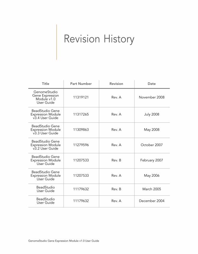
Revision History
Title Part Number Revision Date
GenomeStudio Gene Expression
Module v1.0 User Guide
11319121 Rev. A November 2008
BeadStudio Gene Expression Module
v3.4 User Guide11317265 Rev. A July 2008
BeadStudio Gene Expression Module
v3.3 User Guide11309863 Rev. A May 2008
BeadStudio Gene Expression Module
v3.2 User Guide11279596 Rev. A October 2007
BeadStudio Gene Expression Module
User Guide11207533 Rev. B February 2007
BeadStudio Gene Expression Module
User Guide11207533 Rev. A May 2006
BeadStudio User Guide
11179632 Rev. B March 2005
BeadStudio User Guide
11179632 Rev. A December 2004


Table of Contents
Notice . . . . . . . . . . . . . . . . . . . . . . . . . . . . . . . . . . . . . . . . . . . . . iii
Revision History. . . . . . . . . . . . . . . . . . . . . . . . . . . . . . . . . . . . . . v
Table of Contents . . . . . . . . . . . . . . . . . . . . . . . . . . . . . . . . . . . vii
List of Figures . . . . . . . . . . . . . . . . . . . . . . . . . . . . . . . . . . . . . . .xi
List of Tables . . . . . . . . . . . . . . . . . . . . . . . . . . . . . . . . . . . . . . . xv
Chapter 1 Overview . . . . . . . . . . . . . . . . . . . . . . . . . . . . . . . . . . . 1
Introduction. . . . . . . . . . . . . . . . . . . . . . . . . . . . . . . . . . . . . . . . . 2
Audience and Purpose . . . . . . . . . . . . . . . . . . . . . . . . . . . . . . . . 3
Installing the Gene Expression Module . . . . . . . . . . . . . . . . . . . 3
Gene Expression Module Workflow . . . . . . . . . . . . . . . . . . . . . . 6
Chapter 2 Creating a New Project . . . . . . . . . . . . . . . . . . . . . . . . 9
Introduction. . . . . . . . . . . . . . . . . . . . . . . . . . . . . . . . . . . . . . . . 10
Creating a Project . . . . . . . . . . . . . . . . . . . . . . . . . . . . . . . . . . . 11
Starting the Gene Expression Module . . . . . . . . . . . . . . . . 11
Selecting an Assay Type. . . . . . . . . . . . . . . . . . . . . . . . . . . 12
Choosing a Project Location. . . . . . . . . . . . . . . . . . . . . . . . 13
Selecting Project Data . . . . . . . . . . . . . . . . . . . . . . . . . . . . 15
Defining Groupsets and Groups. . . . . . . . . . . . . . . . . . . . . 20
Defining the Analysis Type and Parameters . . . . . . . . . . . . 26
Creating a Mask File . . . . . . . . . . . . . . . . . . . . . . . . . . . . . . 35
Applying a Group Layout File. . . . . . . . . . . . . . . . . . . . . . . 36
Chapter 3 Viewing Your Data . . . . . . . . . . . . . . . . . . . . . . . . . . . 39
Introduction. . . . . . . . . . . . . . . . . . . . . . . . . . . . . . . . . . . . . . . . 40
GenomeStudio Gene Expression Module v1.0 User Guide
viii Table of Contents
Scatter Plots. . . . . . . . . . . . . . . . . . . . . . . . . . . . . . . . . . . . . . . . 40
Control Panel . . . . . . . . . . . . . . . . . . . . . . . . . . . . . . . . . . . 43
Tools Menu . . . . . . . . . . . . . . . . . . . . . . . . . . . . . . . . . . . . . 46
Context Menu . . . . . . . . . . . . . . . . . . . . . . . . . . . . . . . . . . .48
Finding Items . . . . . . . . . . . . . . . . . . . . . . . . . . . . . . . . . . . 51
Viewing Marked Data . . . . . . . . . . . . . . . . . . . . . . . . . . . . . 59
Viewing Marked Data in a Web Browser . . . . . . . . . . . . . . 60
Saving Marked Data in a Text File . . . . . . . . . . . . . . . . . . . 62
Showing Item Labels in a Scatter Plot. . . . . . . . . . . . . . . . . 64
Other Scatter Plot Functions . . . . . . . . . . . . . . . . . . . . . . . . 65
Bar Plots. . . . . . . . . . . . . . . . . . . . . . . . . . . . . . . . . . . . . . . . . . . 66
Bar Plot Context Menu . . . . . . . . . . . . . . . . . . . . . . . . . . . . 68
Heat Maps . . . . . . . . . . . . . . . . . . . . . . . . . . . . . . . . . . . . . . . . . 69
Heat Map Tools Menu . . . . . . . . . . . . . . . . . . . . . . . . . . . .71
Heat Map Context Menu . . . . . . . . . . . . . . . . . . . . . . . . . . 72
Cluster Analysis Dendrograms . . . . . . . . . . . . . . . . . . . . . . . . .73
Similarities and Distances . . . . . . . . . . . . . . . . . . . . . . . . . . 74
Analyze Clusters . . . . . . . . . . . . . . . . . . . . . . . . . . . . . . . . . 75
Dendrogram Context Menu Selections . . . . . . . . . . . . . . .80
View the Sub-Tree List Directly in the Dendrogram . . . . . .81
Copy/Paste Clusters . . . . . . . . . . . . . . . . . . . . . . . . . . . . . . . . . 81
From Scatter Plot to Dendrogram. . . . . . . . . . . . . . . . . . . . 81
From Dendrogram to Scatter Plot. . . . . . . . . . . . . . . . . . . . 83
Control Summary Reports . . . . . . . . . . . . . . . . . . . . . . . . . . . . . 85
For the DirectHyb Assay . . . . . . . . . . . . . . . . . . . . . . . . . . . 85
For the DASL Assay. . . . . . . . . . . . . . . . . . . . . . . . . . . . . . . 88
Image Viewer. . . . . . . . . . . . . . . . . . . . . . . . . . . . . . . . . . . . . . . 91
Selecting an Image to View . . . . . . . . . . . . . . . . . . . . . . . . 92
Displaying Overlay Cores . . . . . . . . . . . . . . . . . . . . . . . . . . 95
Changing Image Appearance. . . . . . . . . . . . . . . . . . . . . . . 96
Chapter 4 Normalization and Differential Analysis. . . . . . . . . . . 97
Introduction . . . . . . . . . . . . . . . . . . . . . . . . . . . . . . . . . . . . . . . . 98
Normalization Methods & Algorithms . . . . . . . . . . . . . . . . . . . . 98
Sample Scaling . . . . . . . . . . . . . . . . . . . . . . . . . . . . . . . . . . 99
Average. . . . . . . . . . . . . . . . . . . . . . . . . . . . . . . . . . . . . . . . 99
Quantile . . . . . . . . . . . . . . . . . . . . . . . . . . . . . . . . . . . . . . 100
Cubic Spline . . . . . . . . . . . . . . . . . . . . . . . . . . . . . . . . . . . 101
Rank Invariant . . . . . . . . . . . . . . . . . . . . . . . . . . . . . . . . . . 102
Differential Expression Algorithms . . . . . . . . . . . . . . . . . . . . . 103
Illumina Custom . . . . . . . . . . . . . . . . . . . . . . . . . . . . . . . . 103
Part # 11319121 Rev. A
Table of Contents ix
Mann-Whitney . . . . . . . . . . . . . . . . . . . . . . . . . . . . . . . . . 105
T-Test . . . . . . . . . . . . . . . . . . . . . . . . . . . . . . . . . . . . . . . . 105
Detection P-Value . . . . . . . . . . . . . . . . . . . . . . . . . . . . . . . . . . 106
Whole Genome BeadChips . . . . . . . . . . . . . . . . . . . . . . . 106
DASL, miRNA, VeraCode DASL, and Focused Arrays . . . 107
Chapter 5 Analyzing miRNA Data. . . . . . . . . . . . . . . . . . . . . . . 109
Introduction. . . . . . . . . . . . . . . . . . . . . . . . . . . . . . . . . . . . . . . 110
Importing an Analysis for Comparison . . . . . . . . . . . . . . . . . . 110
Loading a Lookup Table . . . . . . . . . . . . . . . . . . . . . . . . . . . . . 112
Generating a Dendrogram . . . . . . . . . . . . . . . . . . . . . . . . . . . 113
Identifying Correlated miRNA and mRNA Expression Values 114
Viewing miRNA Controls. . . . . . . . . . . . . . . . . . . . . . . . . . . . . 117
Chapter 6 Generating a Final Report . . . . . . . . . . . . . . . . . . . . 119
Introduction. . . . . . . . . . . . . . . . . . . . . . . . . . . . . . . . . . . . . . . 120
Generating a Final Report. . . . . . . . . . . . . . . . . . . . . . . . . . . . 120
Viewing a Final Report . . . . . . . . . . . . . . . . . . . . . . . . . . . . . . 124
Chapter 7 User Interface Reference . . . . . . . . . . . . . . . . . . . . . 125
Introduction. . . . . . . . . . . . . . . . . . . . . . . . . . . . . . . . . . . . . . . 126
Detachable Docking Windows . . . . . . . . . . . . . . . . . . . . . . . . 126
Line Plot, Group Gene Profile . . . . . . . . . . . . . . . . . . . . . 127
Bar Plot, Group Gene Profile . . . . . . . . . . . . . . . . . . . . . . 127
Samples Table . . . . . . . . . . . . . . . . . . . . . . . . . . . . . . . . . 128
Group Gene Profile . . . . . . . . . . . . . . . . . . . . . . . . . . . . . 130
Group Probe Profile . . . . . . . . . . . . . . . . . . . . . . . . . . . . . 135
Sample Gene Profile . . . . . . . . . . . . . . . . . . . . . . . . . . . . 139
Sample Probe Profile . . . . . . . . . . . . . . . . . . . . . . . . . . . . 143
Control Gene Profile. . . . . . . . . . . . . . . . . . . . . . . . . . . . . 146
Control Probe Profile . . . . . . . . . . . . . . . . . . . . . . . . . . . . 149
Excluded and Imputed Probes Table . . . . . . . . . . . . . . . . 151
Control Summary . . . . . . . . . . . . . . . . . . . . . . . . . . . . . . . 153
Project Window . . . . . . . . . . . . . . . . . . . . . . . . . . . . . . . . 157
Log Window . . . . . . . . . . . . . . . . . . . . . . . . . . . . . . . . . . . 157
Main Window Menus . . . . . . . . . . . . . . . . . . . . . . . . . . . . . . . 159
Context Menus . . . . . . . . . . . . . . . . . . . . . . . . . . . . . . . . . . . . 163
GenomeStudio Gene Expression Module v1.0 User Guide
x Table of Contents
Appendix A Sample Sheet Format . . . . . . . . . . . . . . . . . . . . . . . 165
Introduction . . . . . . . . . . . . . . . . . . . . . . . . . . . . . . . . . . . . . . . 166
Data Section . . . . . . . . . . . . . . . . . . . . . . . . . . . . . . . . . . . . . . 166
Sample Sheet Template . . . . . . . . . . . . . . . . . . . . . . . . . . . . . 168
Sample Sheet Example . . . . . . . . . . . . . . . . . . . . . . . . . . . . . . 168
Appendix B Troubleshooting . . . . . . . . . . . . . . . . . . . . . . . . . . . 169
Introduction . . . . . . . . . . . . . . . . . . . . . . . . . . . . . . . . . . . . . . . 169
Frequently Asked Questions . . . . . . . . . . . . . . . . . . . . . . . . . . 169
Part # 11319121 Rev. A
List of Figures
Figure 1 GenomeStudio Application Suite Unzipping . . . . . . . . . . . . . . . 3
Figure 2 Selecting GenomeStudio Software Modules . . . . . . . . . . . . . . . 4
Figure 3 License Agreement . . . . . . . . . . . . . . . . . . . . . . . . . . . . . . . . . . . 5
Figure 4 Installing GenomeStudio . . . . . . . . . . . . . . . . . . . . . . . . . . . . . . 5
Figure 5 Installation Complete . . . . . . . . . . . . . . . . . . . . . . . . . . . . . . . . . 6
Figure 6 Gene Expression Analysis Workflow . . . . . . . . . . . . . . . . . . . . . . 7
Figure 7 Project Wizard - Welcome. . . . . . . . . . . . . . . . . . . . . . . . . . . . . 12
Figure 8 Project Wizard - Gene Expression Assay Type . . . . . . . . . . . . . 13
Figure 9 Project Wizard - Project Location . . . . . . . . . . . . . . . . . . . . . . . 14
Figure 10 Project Wizard - Project Data Selection, Repository . . . . . . . . . 15
Figure 11 Project Wizard - Project Data Selection, Sentrix Array Products17
Figure 12 Project Wizard - Project Data Selection, Selected Samples . . . 18
Figure 13 Copying Project Data to Local Storage Location . . . . . . . . . . . 19
Figure 14 GenomeStudio GX Content Descriptors . . . . . . . . . . . . . . . . . 19
Figure 15 Project Wizard - Groupset Definition,
Assigning a Groupset Name. . . . . . . . . . . . . . . . . . . . . . . . . . . 21
Figure 16 Project Wizard - Groupset Definition,
Selecting a Sentrix Array Product . . . . . . . . . . . . . . . . . . . . . . . 22
Figure 17 Project Wizard - Groupset Definition, Selecting Samples. . . . . 23
Figure 18 Project Wizard - Groupset Definition, Defining Project Groups 24
Figure 19 Project Analysis Type and Parameters . . . . . . . . . . . . . . . . . . . 25
Figure 20 Analysis Tables Dialog Box . . . . . . . . . . . . . . . . . . . . . . . . . . . . 26
Figure 21 Select Common Sample File for Sample Plate Scaling
Dialog Box . . . . . . . . . . . . . . . . . . . . . . . . . . . . . . . . . . . . . . . . 29
Figure 22 Example Common Sample File. . . . . . . . . . . . . . . . . . . . . . . . . 30
Figure 23 Sample Plate Scaling Warning . . . . . . . . . . . . . . . . . . . . . . . . . 31
Figure 24 GenomeStudio Progress Status . . . . . . . . . . . . . . . . . . . . . . . . 31
Figure 25 Missing Bead Types . . . . . . . . . . . . . . . . . . . . . . . . . . . . . . . . . 32
Figure 26 GenomeStudio Gene Expression Analysis Results . . . . . . . . . . 34
Figure 27 Excluded and Imputed Probes Table . . . . . . . . . . . . . . . . . . . . 34
Figure 28 Group Layout File Example. . . . . . . . . . . . . . . . . . . . . . . . . . . . 36
Figure 29 Open Dialog Box . . . . . . . . . . . . . . . . . . . . . . . . . . . . . . . . . . . 37
GenomeStudio Gene Expression Module v1.0 User Guide
xii List of Figures
Figure 30 Plot Columns Dialog Box. . . . . . . . . . . . . . . . . . . . . . . . . . . . . . 41
Figure 31 Scatter Plot . . . . . . . . . . . . . . . . . . . . . . . . . . . . . . . . . . . . . . . . 42
Figure 32 Scatter Plot Tools Menu . . . . . . . . . . . . . . . . . . . . . . . . . . . . . . 45
Figure 33 Scatter Plot Context Menu . . . . . . . . . . . . . . . . . . . . . . . . . . . .48
Figure 34 Find Items Tool . . . . . . . . . . . . . . . . . . . . . . . . . . . . . . . . . . . . . 51
Figure 35 Find Items Dialog Box . . . . . . . . . . . . . . . . . . . . . . . . . . . . . . . .52
Figure 36 Zoom in to See Selected Genes . . . . . . . . . . . . . . . . . . . . . . . . 54
Figure 37 Gene Properties, Data Tab . . . . . . . . . . . . . . . . . . . . . . . . . . . .55
Figure 38 Gene Properties, Manifest Tab . . . . . . . . . . . . . . . . . . . . . . . . .56
Figure 39 NCBI Website . . . . . . . . . . . . . . . . . . . . . . . . . . . . . . . . . . . . . .57
Figure 40 NCBI Record for the Selected Gene . . . . . . . . . . . . . . . . . . . . . 58
Figure 41 Gene Properties, Ontology Tab . . . . . . . . . . . . . . . . . . . . . . . . 59
Figure 42 Scatter Plot Context Menu, Marked List Options . . . . . . . . . . . 60
Figure 43 GenomeStudio Scatter Plot Output Data Dialog Box . . . . . . . . 61
Figure 44 Marked Data Shown in a Web Browser . . . . . . . . . . . . . . . . . . .62
Figure 45 Save Marked Genes List As . . . . . . . . . . . . . . . . . . . . . . . . . . . . 62
Figure 46 GenomeStudio Scatter Plot Output Data Dialog Box . . . . . . . . 63
Figure 47 Saving Marked Data in a Text File. . . . . . . . . . . . . . . . . . . . . . . 64
Figure 48 Selecting a Label for a Scatter Plot . . . . . . . . . . . . . . . . . . . . . . 64
Figure 49 Showing Item Labels for Marked Data in a Scatter Plot . . . . . . 65
Figure 50 Bar Plot of Sample Probe Profile . . . . . . . . . . . . . . . . . . . . . . . . 66
Figure 51 Plot Settings Dialog Box . . . . . . . . . . . . . . . . . . . . . . . . . . . . . . 67
Figure 52 Bar Plot With User-Selected Attributes . . . . . . . . . . . . . . . . . . .68
Figure 53 Bar Plot Context Menu . . . . . . . . . . . . . . . . . . . . . . . . . . . . . . . 68
Figure 54 Creating a Heat Map . . . . . . . . . . . . . . . . . . . . . . . . . . . . . . . . . 70
Figure 55 Heat Map. . . . . . . . . . . . . . . . . . . . . . . . . . . . . . . . . . . . . . . . . . 71
Figure 56 Heat Map Tools Menu . . . . . . . . . . . . . . . . . . . . . . . . . . . . . . . .71
Figure 57 Heat Map Context Menu. . . . . . . . . . . . . . . . . . . . . . . . . . . . . . 72
Figure 58 Dendrogram Similarity Example . . . . . . . . . . . . . . . . . . . . . . . . 75
Figure 59 Dendrogram, Showing Nodes. . . . . . . . . . . . . . . . . . . . . . . . . . 75
Figure 60 Cluster Analysis Dialog Box. . . . . . . . . . . . . . . . . . . . . . . . . . . . 77
Figure 61 Clustering Progress Status. . . . . . . . . . . . . . . . . . . . . . . . . . . . . 78
Figure 62 Dendrogram . . . . . . . . . . . . . . . . . . . . . . . . . . . . . . . . . . . . . . . 78
Figure 63 Dendrogram with Context Menu. . . . . . . . . . . . . . . . . . . . . . . . 79
Figure 64 Zooming In to View a Sub-Tree List . . . . . . . . . . . . . . . . . . . . . 81
Figure 65 Selecting a Region. . . . . . . . . . . . . . . . . . . . . . . . . . . . . . . . . . .82
Figure 66 Selecting a Sub-Tree . . . . . . . . . . . . . . . . . . . . . . . . . . . . . . . . . 84
Figure 67 Copying a Sub-Tree . . . . . . . . . . . . . . . . . . . . . . . . . . . . . . . . . 85
Figure 68 Control Summary Report . . . . . . . . . . . . . . . . . . . . . . . . . . . . . . 86
Figure 69 Housekeeping Controls Secondary Graph . . . . . . . . . . . . . . . . 87
Figure 70 Control Summary Context Menu. . . . . . . . . . . . . . . . . . . . . . . . 88
Figure 71 Control Summary Report . . . . . . . . . . . . . . . . . . . . . . . . . . . . . . 89
Part # 11319121 Rev. A
List of Figures xiii
Figure 72 Contamination Controls Secondary Graph . . . . . . . . . . . . . . . . 90
Figure 73 Control Summary Context Menu . . . . . . . . . . . . . . . . . . . . . . . 91
Figure 74 GenomeStudio View Image . . . . . . . . . . . . . . . . . . . . . . . . . . . 92
Figure 75 Image Viewer . . . . . . . . . . . . . . . . . . . . . . . . . . . . . . . . . . . . . . 93
Figure 76 Overlay Cores . . . . . . . . . . . . . . . . . . . . . . . . . . . . . . . . . . . . . . 95
Figure 77 Image Control Pane . . . . . . . . . . . . . . . . . . . . . . . . . . . . . . . . . 96
Figure 78 Select Analysis | Import Analysis . . . . . . . . . . . . . . . . . . . . . . . 110
Figure 79 Import Analysis Wizard . . . . . . . . . . . . . . . . . . . . . . . . . . . . . . 111
Figure 80 Example Lookup Table . . . . . . . . . . . . . . . . . . . . . . . . . . . . . . 112
Figure 81 Group Gene Profile Dialog Box . . . . . . . . . . . . . . . . . . . . . . . 113
Figure 82 Dendrogram Generated with the Clustering Tool . . . . . . . . . 114
Figure 83 Dendrogram and Related Data Table. . . . . . . . . . . . . . . . . . . 115
Figure 84 Line Plots and Dendrograms Showing Anticorrelation Between
miRNA and mRNA Expression Levels . . . . . . . . . . . . . . . . . . . 116
Figure 85 miRNA Assay Control Plots . . . . . . . . . . . . . . . . . . . . . . . . . . . 117
Figure 86 Creating a Final Report . . . . . . . . . . . . . . . . . . . . . . . . . . . . . . 120
Figure 87 GenomeStudio Gene Expression Reports . . . . . . . . . . . . . . . 121
Figure 88 Final Report Dialog Box . . . . . . . . . . . . . . . . . . . . . . . . . . . . . 122
Figure 89 Selecting Options for the Final Report . . . . . . . . . . . . . . . . . . 122
Figure 90 Saving the Final Report . . . . . . . . . . . . . . . . . . . . . . . . . . . . . . 123
Figure 91 Naming the Final Report. . . . . . . . . . . . . . . . . . . . . . . . . . . . . 123
Figure 92 Final Report. . . . . . . . . . . . . . . . . . . . . . . . . . . . . . . . . . . . . . . 124
Figure 93 Gene Expression Module Default View . . . . . . . . . . . . . . . . . 126
Figure 94 Line Plot, Group Gene Profile . . . . . . . . . . . . . . . . . . . . . . . . . 127
Figure 95 Bar Plot, Group Gene Profile . . . . . . . . . . . . . . . . . . . . . . . . . 128
Figure 96 Samples Table. . . . . . . . . . . . . . . . . . . . . . . . . . . . . . . . . . . . . 128
Figure 97 Group Gene Profile . . . . . . . . . . . . . . . . . . . . . . . . . . . . . . . . . 131
Figure 98 Group Probe Profile . . . . . . . . . . . . . . . . . . . . . . . . . . . . . . . . 135
Figure 99 Sample Gene Profile . . . . . . . . . . . . . . . . . . . . . . . . . . . . . . . . 139
Figure 100 Sample Probe Profile . . . . . . . . . . . . . . . . . . . . . . . . . . . . . . . 143
Figure 101 Control Gene Profile . . . . . . . . . . . . . . . . . . . . . . . . . . . . . . . . 147
Figure 102 Control Probe Profile . . . . . . . . . . . . . . . . . . . . . . . . . . . . . . . 149
Figure 103 Excluded and Imputed Probes Table . . . . . . . . . . . . . . . . . . . 151
Figure 104 Control Summary, Direct Hyb . . . . . . . . . . . . . . . . . . . . . . . . . 153
Figure 105 Control Summary, DASL . . . . . . . . . . . . . . . . . . . . . . . . . . . . . 154
Figure 106 Control Summary, Whole Genome DASL. . . . . . . . . . . . . . . . 155
Figure 107 Control Summary, miRNA. . . . . . . . . . . . . . . . . . . . . . . . . . . . 156
Figure 108 Project Window. . . . . . . . . . . . . . . . . . . . . . . . . . . . . . . . . . . . 157
Figure 109 Log Window . . . . . . . . . . . . . . . . . . . . . . . . . . . . . . . . . . . . . . 157
Figure 110 Sample Sheet Example . . . . . . . . . . . . . . . . . . . . . . . . . . . . . . 168
GenomeStudio Gene Expression Module v1.0 User Guide

GenomeStudio Gene Expression Module v1.0 User Guide
List of Tables
Table 1 Scatter Plot Control Panel Functions & Descriptions . . . . . . . . 43
Table 2 Scatter Plot Tools Menu Item Descriptions. . . . . . . . . . . . . . . . 46
Table 3 Scatter Plot Context Menu Item Descriptions. . . . . . . . . . . . . . 48
Table 4 Bar Plot Context Menu Item Descriptions. . . . . . . . . . . . . . . . . 69
Table 5 Heat Map Tools Menu Item Descriptions . . . . . . . . . . . . . . . . . 72
Table 6 Heat Map Context Menu Item Descriptions . . . . . . . . . . . . . . . 73
Table 7 Dendrogram Context Menu Selections . . . . . . . . . . . . . . . . . . 80
Table 8 Image Viewer Features . . . . . . . . . . . . . . . . . . . . . . . . . . . . . . . 93
Table 9 Control Features for the miRNA Assay . . . . . . . . . . . . . . . . . . 118
Table 10 Samples Table Columns . . . . . . . . . . . . . . . . . . . . . . . . . . . . . 129
Table 11 Group Gene Profile Columns . . . . . . . . . . . . . . . . . . . . . . . . . 132
Table 12 Group Gene Profile Per-Group Columns . . . . . . . . . . . . . . . . 134
Table 13 Group Probe Profile Columns . . . . . . . . . . . . . . . . . . . . . . . . . 136
Table 14 Group Probe Profile Per-Group Columns . . . . . . . . . . . . . . . . 138
Table 15 Sample Gene Profile Columns . . . . . . . . . . . . . . . . . . . . . . . . 140
Table 16 Sample Gene Profile Per-Sample Columns. . . . . . . . . . . . . . . 142
Table 17 Sample Probe Profile Columns . . . . . . . . . . . . . . . . . . . . . . . . 144
Table 18 Sample Probe Profile Per-Sample Columns . . . . . . . . . . . . . . 146
Table 19 Control Gene Profile Columns . . . . . . . . . . . . . . . . . . . . . . . . 148
Table 20 Control Gene Profile Per-Sample Columns. . . . . . . . . . . . . . . 148
Table 21 Control Probe Profile Columns . . . . . . . . . . . . . . . . . . . . . . . . 150
Table 22 Control Probe Profile Per-Sample Columns . . . . . . . . . . . . . . 150
Table 23 Excluded and Imputed Probes Table Columns . . . . . . . . . . . 152
Table 24 Excluded and Imputed Probes Table Per-Sample Columns . . 152
Table 25 Log Window Selections & Functions. . . . . . . . . . . . . . . . . . . . 158
Table 26 Main Menu Selections & Functions. . . . . . . . . . . . . . . . . . . . . 159
Table 27 Bar Plot: Group Gene Profile Window Context Menu . . . . . . 163
Table 28 Other Tabbed Window Context Menu . . . . . . . . . . . . . . . . . . 163
Table 29 Project Window Context Menu . . . . . . . . . . . . . . . . . . . . . . . . 164
Table 30 Log Window Context Menu . . . . . . . . . . . . . . . . . . . . . . . . . . 164
Table 31 Data Section, Optional and Required Columns . . . . . . . . . . . 166
Table 32 Frequently Asked Questions. . . . . . . . . . . . . . . . . . . . . . . . . . 169


Chapter 1
Overview
Topics2 Introduction
3 Audience and Purpose
3 Installing the Gene Expression Module
6 Gene Expression Module Workflow
GenomeStudio Gene Expression Module v1.0 User Guide
2 CHAPTER 1
Overview
Introduction
The GenomeStudio Gene Expression Module is a tool for
analyzing gene expression data from scanned microarray images
generated by the Illumina BeadArrayTM Reader, or scanned
intensity data generated by the Illumina BeadXpress® Reader.
You can use the resulting GenomeStudio output files with most
standard gene expression analysis programs.
The GenomeStudio Gene Expression Module allows you to
examine data generated from the following assays:
Direct Hyb Assay
DASL® Assay
VeraCode® DASL Assay
Whole Genome DASL Assay
miRNA Assay
In addition, it enables two types of data analysis:
Gene Analysis—quantifying gene expression signal levels
Differential Analysis—determining whether gene expression
levels have changed between two experimental groups
You can perform analyses on individual samples or on groups of
samples treated as replicates.
The Gene Expression Module reports experiment performance
based on built-in controls that accompany each experiment. In
addition, this module includes the following tools, which provide
a quick, visual means for exploratory analysis:
Line plots
Scatter plots
Histograms
Dendrograms
Box plots
Heat maps
Samples table
Image viewer
Illumina Genome Viewer (IGV)
Illumina Chromosome Browser (ICB)
Part # 11319121 Rev. A
Audience and Purpose 3
Audience and Purpose
This guide is written for researchers who want to use the
GenomeStudio Gene Expression Module to analyze data
generated by performing Illumina’s DirectHyb, miRNA, DASL,
Whole-Genome DASL, or VeraCode DASL assays.
This guide includes procedures and user interface information
specific to the GenomeStudio Gene Expression Module. For
information about the GenomeStudio Framework, the common
user interface and functionality available in all GenomeStudio
Modules, refer to the GenomeStudio Framework User Guide.
Installing the Gene Expression Module
To install the GenomeStudio Gene Expression Module:
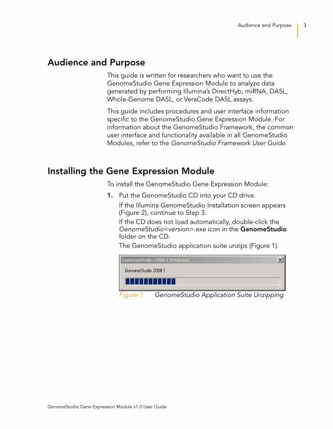
1. Put the GenomeStudio CD into your CD drive.
If the Illumina GenomeStudio Installation screen appears (Figure 2), continue to Step 3.
If the CD does not load automatically, double-click the GenomeStudio<version>.exe icon in the GenomeStudio folder on the CD.
The GenomeStudio application suite unzips (Figure 1).
Figure 1 GenomeStudio Application Suite Unzipping
GenomeStudio Gene Expression Module v1.0 User Guide
4 CHAPTER 1
Overview
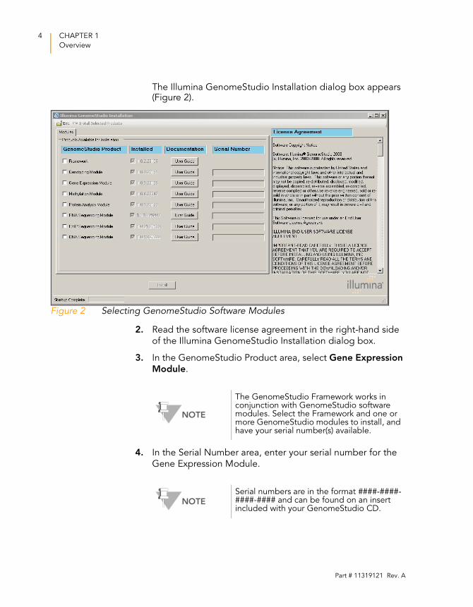
The Illumina GenomeStudio Installation dialog box appears (Figure 2).
Figure 2 Selecting GenomeStudio Software Modules
2. Read the software license agreement in the right-hand side
of the Illumina GenomeStudio Installation dialog box.
3. In the GenomeStudio Product area, select Gene Expression
Module.
4. In the Serial Number area, enter your serial number for the
Gene Expression Module.
NOTE
The GenomeStudio Framework works in conjunction with GenomeStudio software modules. Select the Framework and one or more GenomeStudio modules to install, and have your serial number(s) available.
NOTE
Serial numbers are in the format ####-####-####-#### and can be found on an insert included with your GenomeStudio CD.
Part # 11319121 Rev. A
Installing the Gene Expression Module 5
5. [Optional] Enter the serial numbers for additional
GenomeStudio modules if you have licenses for additional
GenomeStudio modules and want to install them now.
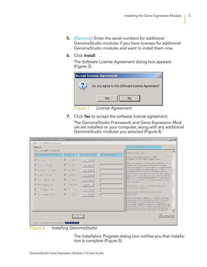
6. Click Install.
The Software License Agreement dialog box appears (Figure 3).
Figure 3 License Agreement
7. Click Yes to accept the software license agreement.
The GenomeStudio Framework and Gene Expression Mod-ule are installed on your computer, along with any additional GenomeStudio modules you selected (Figure 4).
Figure 4 Installing GenomeStudio
The Installation Progress dialog box notifies you that installa-tion is complete (Figure 5).
GenomeStudio Gene Expression Module v1.0 User Guide
6 CHAPTER 1
Overview
Figure 5 Installation Complete
8. Click OK.
9. In the Illumina GenomeStudio Installation dialog box (Figure
4), click Exit.
You can now start a new GenomeStudio project using any GenomeStudio module you have installed.
See Chapter 2, Creating a New Project, for information
about starting a new Gene Expression project.
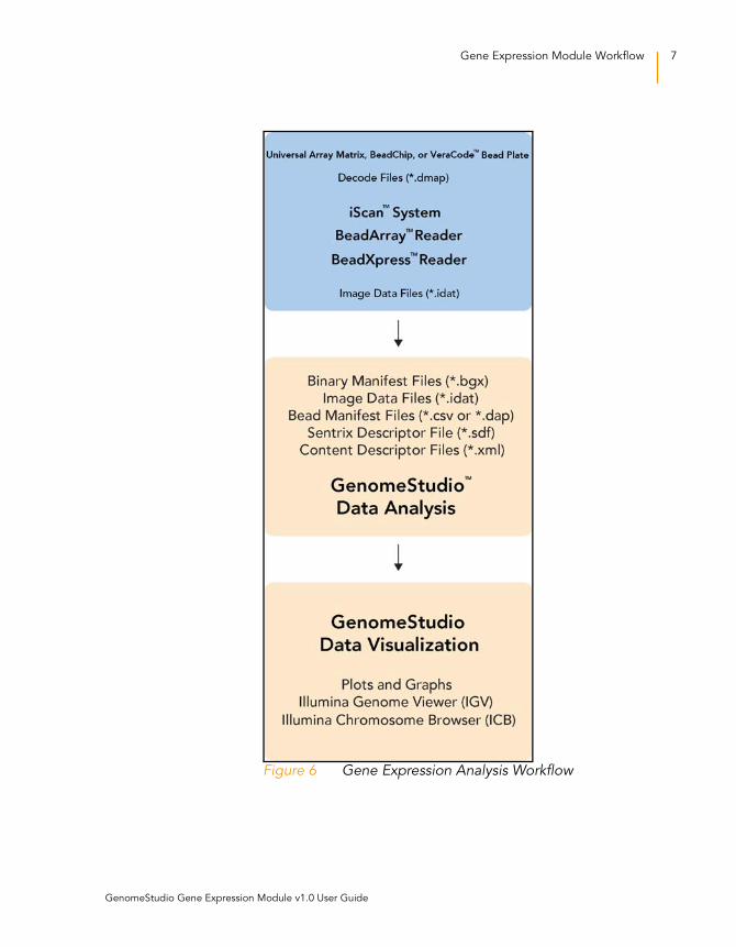
Gene Expression Module Workflow
The basic workflow for gene expression analysis using Illumina’s
GenomeStudio Gene Expression Module is summarized in
Figure 6.
Part # 11319121 Rev. A
Gene Expression Module Workflow 7
Figure 6 Gene Expression Analysis Workflow
GenomeStudio Gene Expression Module v1.0 User Guide

8 CHAPTER 1
Overview
Part # 11319121 Rev. A

Chapter 2
Creating a New Project
Topics10 Introduction
11 Creating a Project
11 Starting the Gene Expression Module
12 Selecting an Assay Type
13 Choosing a Project Location
15 Selecting Project Data
20 Defining Groupsets and Groups
26 Defining the Analysis Type and Parameters
35 Creating a Mask File
GenomeStudio Gene Expression Module v1.0 User Guide
10 CHAPTER 2
Creating a New Project
Introduction
Using intensity (*.idat) files produced by the BeadArray Reader
or BeadXpress Reader, the Gene Expression Module’s gene
analysis tools produce data tables containing:
Probe and gene lists
Associated signal intensities (normalized or raw)
Information about system controls
In addition, the Gene Expression Module’s differential analysis
tools can produce data tables displaying the probability that a
gene's signal has changed between two samples or groups of
samples.
Using GenomeStudio's data visualization tools, you can create
sophisticated plotting analyses, including:
Line plots
Scatter plots
Bar plots
Box plots
Heat maps
Histograms
Cluster analysis dendrograms
To run a gene expression analysis, you must first create a
GenomeStudio project. In a project, you define one or more
groupsets, one or more groups (sample sets that can be
compared against each other for the purpose of identifying
differences in gene expression), and one or more analyses. For
more information about groupsets and groups, see Defining Groupsets and Groups later in this chapter.
In the simplest experiment, each group may have only one
sample. However, if your experiment includes replicate samples,
you can assign these to the same group.
In a project and within a group, GenomeStudio averages the
values for each gene across the samples, and algorithms
automatically take advantage of beadtype replicates to provide
accurate estimates of relative mRNA abundance. This translates
into a highly sensitive determination of detection and differential
expression.
Part # 11319121 Rev. A

Creating a Project 11
The following section, Creating a Project, provides step-by-step
instructions for the following tasks:
Defining a project
Creating groupsets and groups
Defining analysis type and parameters
Applying normalization and differential
expression algorithms
Viewing and analyzing your data
The GenomeStudio Project Wizard guides you through creating
a project, while the GenomeStudio main page provides a
starting-point from which you can carry out the same functions
independently.
Creating a Project
Follow the instructions in this section to create a GenomeStudio
project using data from Illumina’s Direct Hyb, DASL, VeraCode
DASL, Whole Genome DASL, or miRNA assays with the
GenomeStudio Project Wizard.
Starting theGene
ExpressionModule
1. In GenomeStudio, open the Gene Expression Module by
selecting File | New Project | Gene Expression.
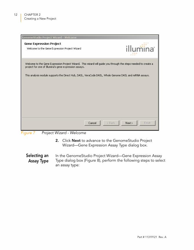
The GenomeStudio Project Wizard—Welcome dialog box
appears (Figure 7).
GenomeStudio Gene Expression Module v1.0 User Guide
12 CHAPTER 2
Creating a New Project
Figure 7 Project Wizard - Welcome
2. Click Next to advance to the GenomeStudio Project
Wizard—Gene Expression Assay Type dialog box.
Selecting anAssay Type
In the GenomeStudio Project Wizard—Gene Expression Assay
Type dialog box (Figure 8), perform the following steps to select
an assay type:
Part # 11319121 Rev. A
Creating a Project 13
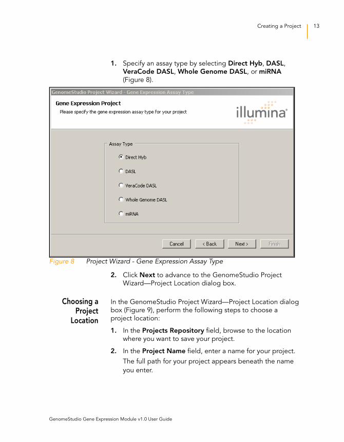
1. Specify an assay type by selecting Direct Hyb, DASL,
VeraCode DASL, Whole Genome DASL, or miRNA
(Figure 8).
Figure 8 Project Wizard - Gene Expression Assay Type
2. Click Next to advance to the GenomeStudio Project
Wizard—Project Location dialog box.
Choosing aProject
Location
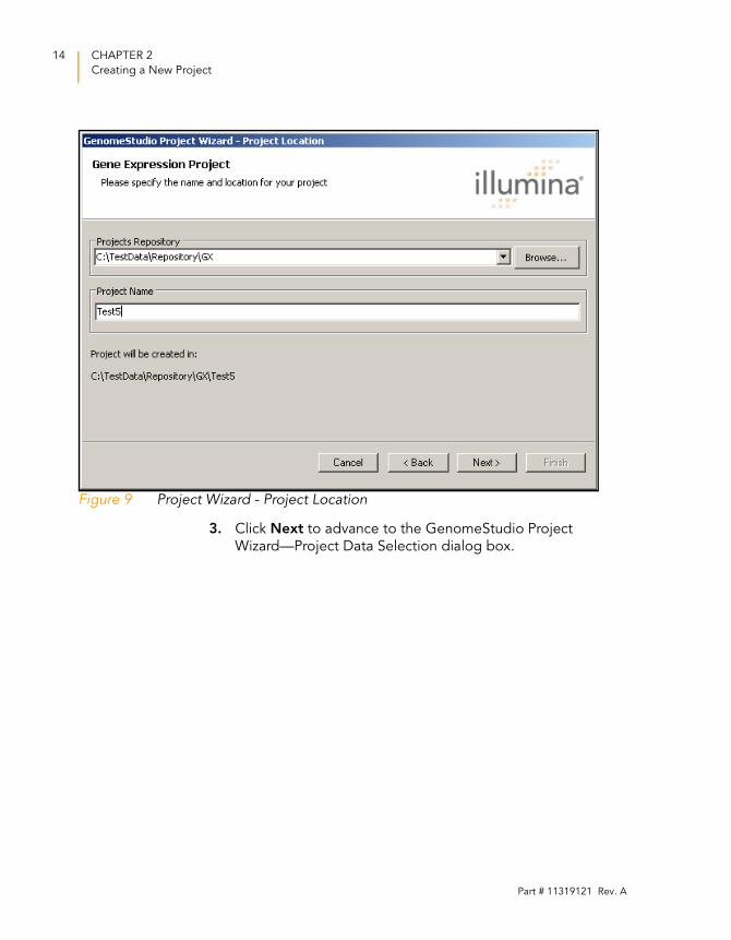
In the GenomeStudio Project Wizard—Project Location dialog
box (Figure 9), perform the following steps to choose a
project location:
1. In the Projects Repository field, browse to the location
where you want to save your project.
2. In the Project Name field, enter a name for your project.
The full path for your project appears beneath the name
you enter.
GenomeStudio Gene Expression Module v1.0 User Guide
14 CHAPTER 2
Creating a New Project
Figure 9 Project Wizard - Project Location
3. Click Next to advance to the GenomeStudio Project
Wizard—Project Data Selection dialog box.
Part # 11319121 Rev. A
Creating a Project 15
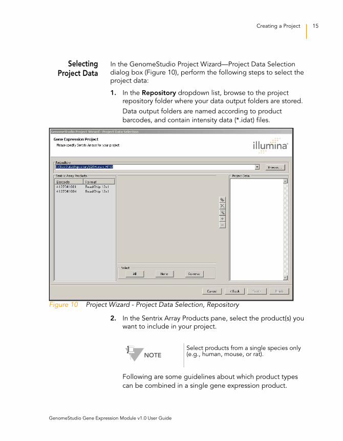
SelectingProject Data
In the GenomeStudio Project Wizard—Project Data Selection
dialog box (Figure 10), perform the following steps to select the
project data:
1. In the Repository dropdown list, browse to the project
repository folder where your data output folders are stored.
Data output folders are named according to product
barcodes, and contain intensity data (*.idat) files.
Figure 10 Project Wizard - Project Data Selection, Repository
2. In the Sentrix Array Products pane, select the product(s) you
want to include in your project.
Following are some guidelines about which product types
can be combined in a single gene expression product.
NOTE
Select products from a single species only (e.g., human, mouse, or rat).
GenomeStudio Gene Expression Module v1.0 User Guide
16 CHAPTER 2
Creating a New Project
• Human v2 products can be combined with Human v3
and future human products in a single gene expression
project, but Human v1 products cannot be combined
with Human v2 and future human products.
• Mouse v1.1 products can be combined with future
mouse products in a single gene expression project, but
Mouse v1.0 products cannot be combined with Mouse
v1.1 and future mouse products.
• HumanWG-6 products can be combined with
HumanRef-8 products.
Example 1
HumanWG-6 v2 products
can be combined with
HumanWG-6 v3 products
Example 2
HumanWG-6 v2 products
can be combined with
HumanRef-8 v2 products
Example 3
HumanWG-6 v1 products
cannot be combined with
HumanWG-6 v2 products
Example 4
HumanWG-6 v2 products
cannot be combined with
RatRef-12 v2 products
Example 5
MouseRef-8 v1.0 products
cannot be combined with
Mouse Ref-8 v1.1 products
Part # 11319121 Rev. A
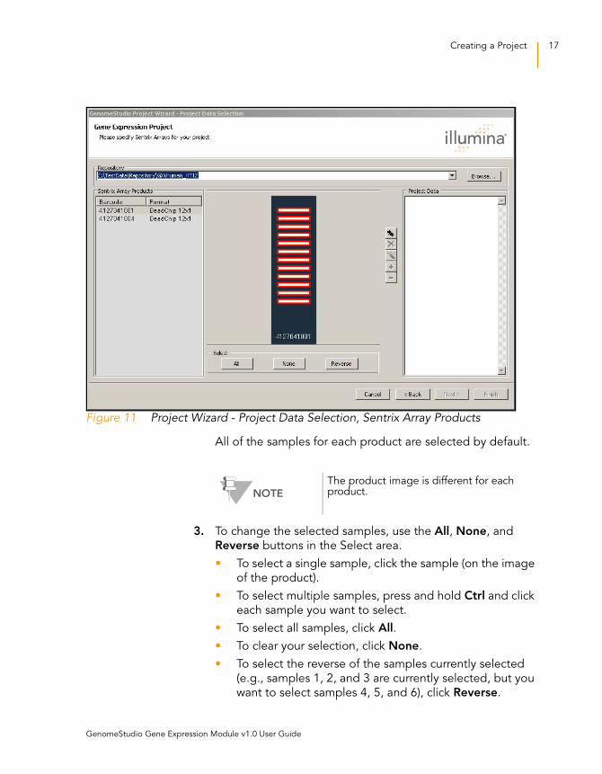
Creating a Project 17
Figure 11 Project Wizard - Project Data Selection, Sentrix Array Products
All of the samples for each product are selected by default.
3. To change the selected samples, use the All, None, and
Reverse buttons in the Select area.
• To select a single sample, click the sample (on the image
of the product).
• To select multiple samples, press and hold Ctrl and click
each sample you want to select.
• To select all samples, click All.
• To clear your selection, click None.
• To select the reverse of the samples currently selected
(e.g., samples 1, 2, and 3 are currently selected, but you
want to select samples 4, 5, and 6), click Reverse.
NOTE
The product image is different for each product.
GenomeStudio Gene Expression Module v1.0 User Guide
18 CHAPTER 2
Creating a New Project
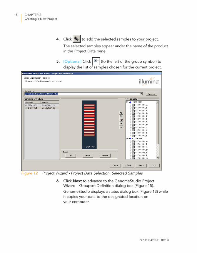
4. Click to add the selected samples to your project.
The selected samples appear under the name of the product
in the Project Data pane.
5. [Optional] Click (to the left of the group symbol) to
display the list of samples chosen for the current project.
Figure 12 Project Wizard - Project Data Selection, Selected Samples
6. Click Next to advance to the GenomeStudio Project
Wizard—Groupset Definition dialog box (Figure 15).
GenomeStudio displays a status dialog box (Figure 13) while
it copies your data to the designated location on
your computer.
Part # 11319121 Rev. A
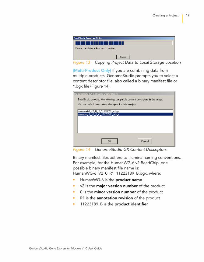
Creating a Project 19
Figure 13 Copying Project Data to Local Storage Location
[Multi-Product Only] If you are combining data from
multiple products, GenomeStudio prompts you to select a
content descriptor file, also called a binary manifest file or
*.bgx file (Figure 14).
Figure 14 GenomeStudio GX Content Descriptors
Binary manifest files adhere to Illumina naming conventions.
For example, for the HumanWG-6 v2 BeadChip, one
possible binary manifest file name is:
HumanWG-6_V2_0_R1_11223189_B.bgx, where:
• HumanWG-6 is the product name
• v2 is the major version number of the product
• 0 is the minor version number of the product
• R1 is the annotation revision of the product
• 11223189_B is the product identifier
GenomeStudio Gene Expression Module v1.0 User Guide
20 CHAPTER 2
Creating a New Project
7. Select a content descriptor file (*.bgx file).
8. Click OK.
The GenomeStudio Project Wizard—Groupset Definition
dialog box appears (Figure 15). Continue to the next section
to define groupsets and groups
DefiningGroupsets and
Groups
GenomeStudio projects are structured in a hierarchical manner:
A project includes one or more groupsets.
A groupset is a collection of one or more groups that you
choose to analyze simultaneously.
A group is a set of arrays that share a functional relationship
(e.g., replicates, zero time points, reference group). Within a
groupset, an array can be included in more than one group,
or it can be analyzed individually.
There are two types of analysis: gene analysis and differential
expression analysis. You perform an analysis on a single
groupset at a time.
Perform the following steps to define a groupset for your project.
1. Assign a name to your groupset by doing one of
the following:
• Click New and enter a name for your new groupset.
• Click Existing and choose the groupset you want from
the dropdown list.
NOTE
Early versions of Illumina Gene Expression products, including Human v1, Human v2, Mouse v1, Mouse v1.1, and RatRef-12 v1, require that you use a text-based content descriptor file (*.xml file) or manifest file (*.csv file) instead of a *.bgx file.
Newer products use binary manifest files, which are more compact. *.bgx files contain additional annotation information, such as chromosomal position, which allows you to view gene expression data in the Illumina Genome Viewer (IGV) and the Illumina Chromosome Browser (ICB).
Part # 11319121 Rev. A
Creating a Project 21
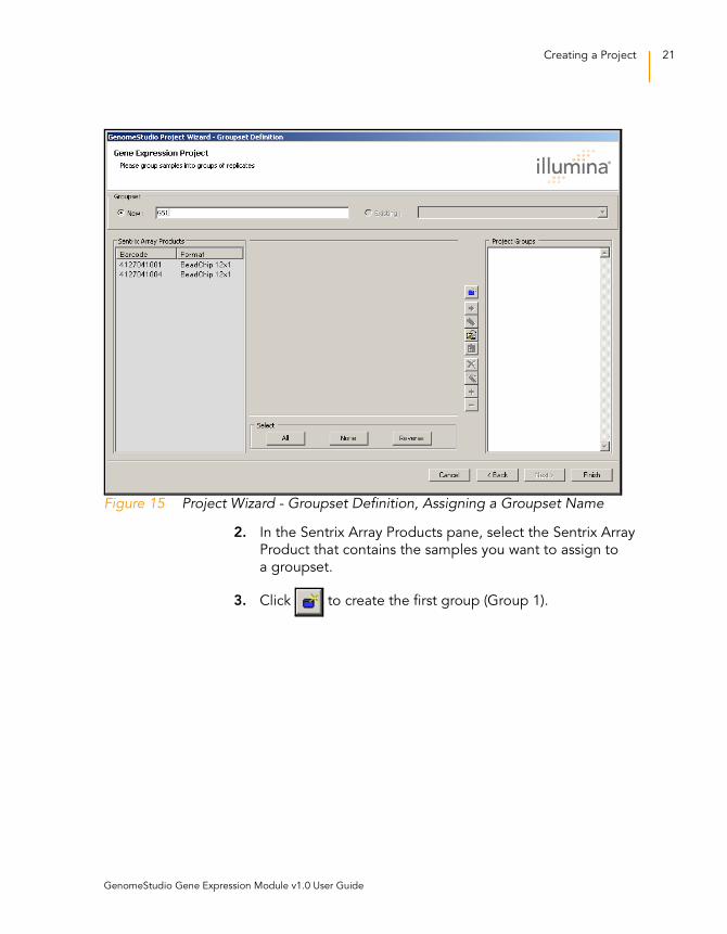
Figure 15 Project Wizard - Groupset Definition, Assigning a Groupset Name
2. In the Sentrix Array Products pane, select the Sentrix Array
Product that contains the samples you want to assign to
a groupset.
3. Click to create the first group (Group 1).
GenomeStudio Gene Expression Module v1.0 User Guide
22 CHAPTER 2
Creating a New Project
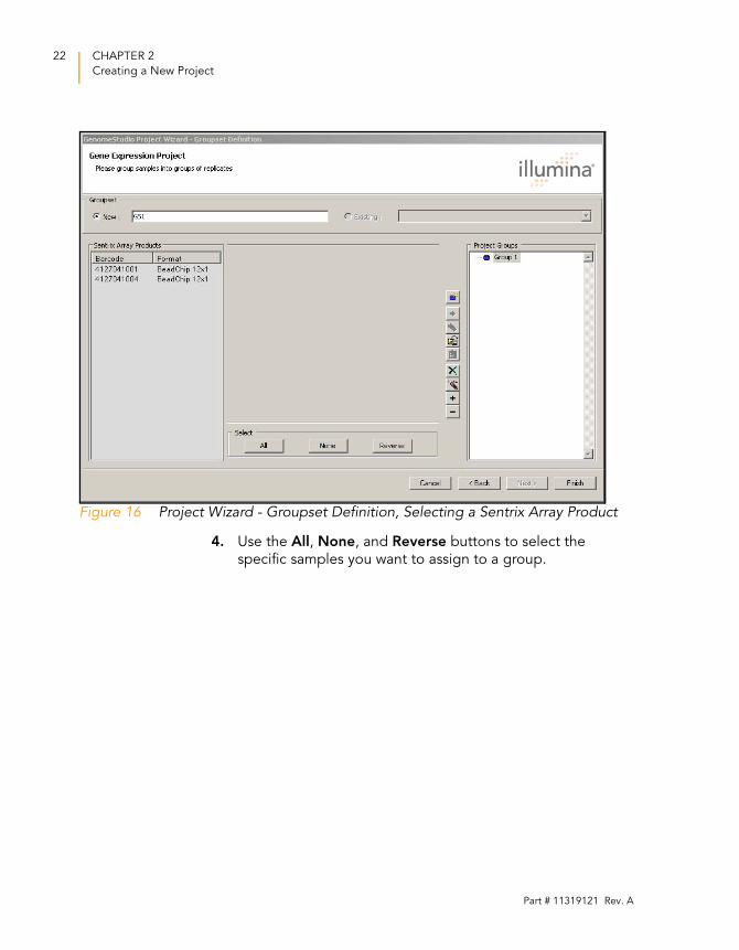
Figure 16 Project Wizard - Groupset Definition, Selecting a Sentrix Array Product
4. Use the All, None, and Reverse buttons to select the
specific samples you want to assign to a group.
Part # 11319121 Rev. A
Creating a Project 23
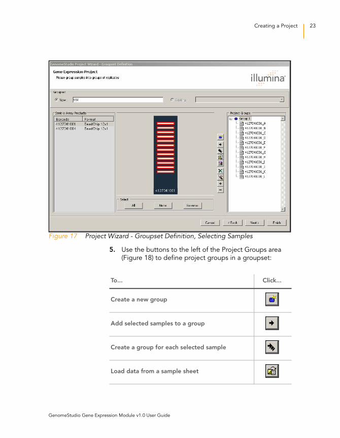
Figure 17 Project Wizard - Groupset Definition, Selecting Samples
5. Use the buttons to the left of the Project Groups area
(Figure 18) to define project groups in a groupset:
To... Click...
Create a new group
Add selected samples to a group
Create a group for each selected sample
Load data from a sample sheet
GenomeStudio Gene Expression Module v1.0 User Guide
24 CHAPTER 2
Creating a New Project
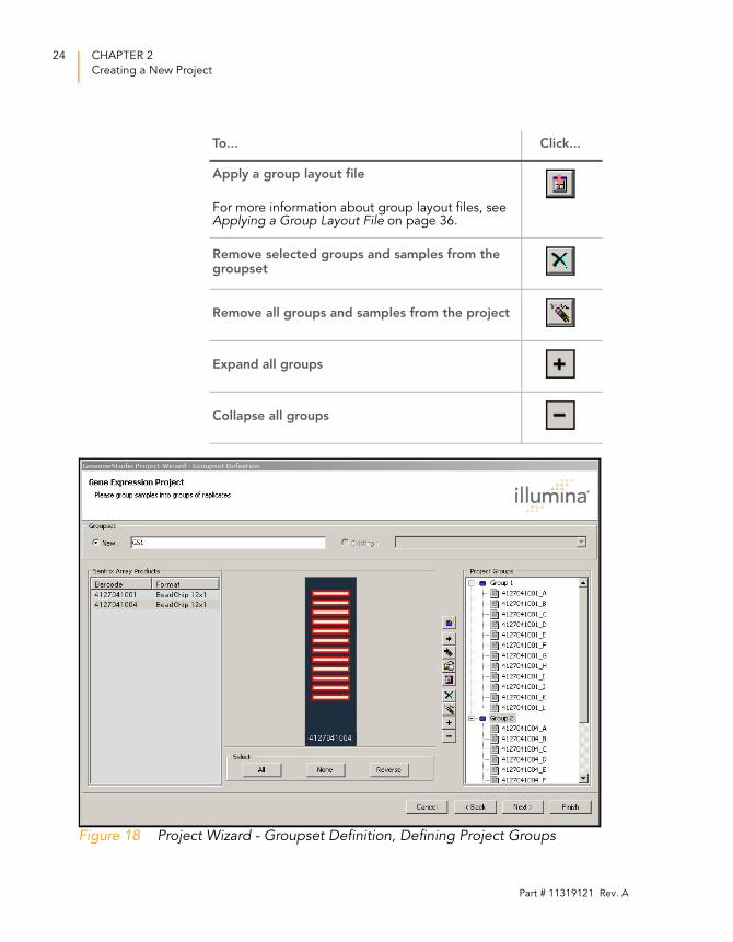
Figure 18 Project Wizard - Groupset Definition, Defining Project Groups
Apply a group layout file
For more information about group layout files, see Applying a Group Layout File on page 36.
Remove selected groups and samples from the groupset
Remove all groups and samples from the project
Expand all groups
Collapse all groups
To... Click...
Part # 11319121 Rev. A
Creating a Project 25
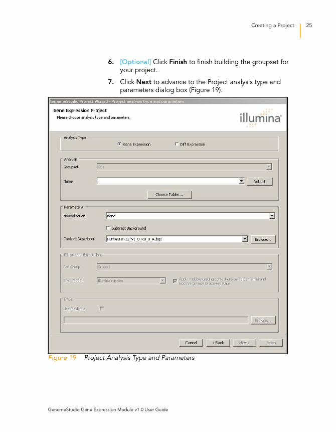
6. [Optional] Click Finish to finish building the groupset for
your project.
7. Click Next to advance to the Project analysis type and
parameters dialog box (Figure 19).
Figure 19 Project Analysis Type and Parameters
GenomeStudio Gene Expression Module v1.0 User Guide
26 CHAPTER 2
Creating a New Project
Defining theAnalysis Type
andParameters
Perform the following steps to define the analysis type
and parameters for your project:
1. In the Analysis Type area, select Gene Expression or
Diff Expression.
2. In the Name area, enter a name for this analysis.
3. Do one of the following:
a. If you want to display the default data tables in this
project, continue to step 6.
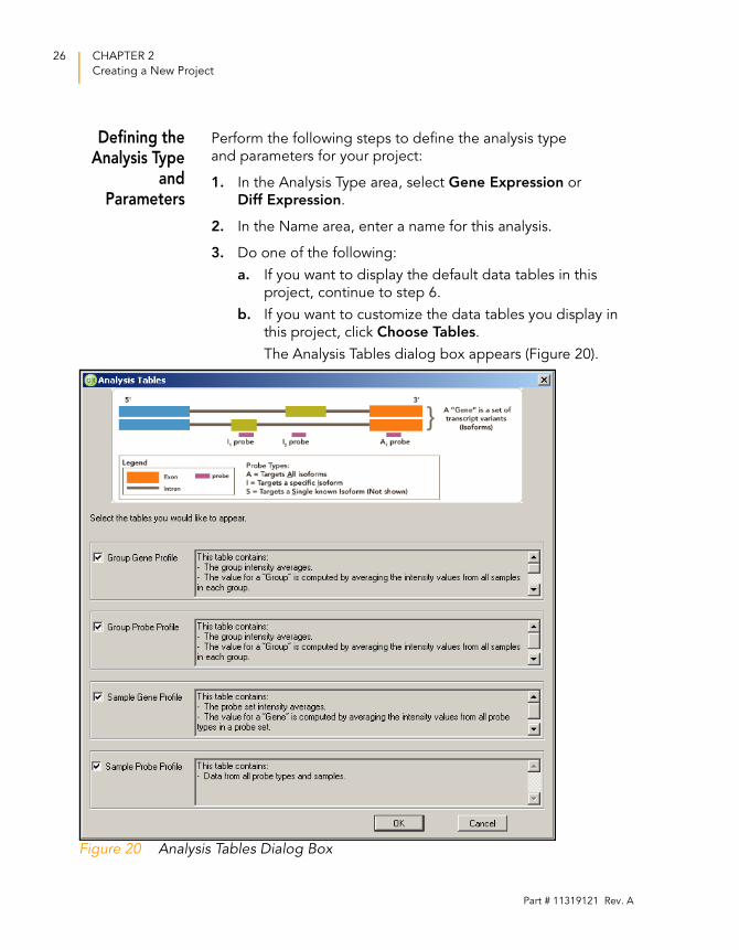
b. If you want to customize the data tables you display in
this project, click Choose Tables.
The Analysis Tables dialog box appears (Figure 20).
Figure 20 Analysis Tables Dialog Box
Part # 11319121 Rev. A
Creating a Project 27
4. Select the tables you want to display in this project.
5. Click OK.
The Analysis Tables dialog box closes. The tables you
selected will appear in your project.
6. On the Project Analysis Type and Parameters dialog box
(Figure 19), in the Parameters area, select the normalization
method you want to use:
• None
• Average
• Quantile
• Rank invariant
• Cubic spline
For information about normalization methods, see
Normalization Methods & Algorithms on page 98.
If you have run a DASL or miRNA assay, you must decide
whether to enable sample plate scaling for this analysis. Sample
plate scaling allows you to address lot-to-lot variation. This
feature works with common samples across multiple BeadChips,
SAMs, or VeraCode Bead Plates.
Sample plate scaling scales the intensities of all probes to create
equal average intensities of all common samples for all plates for
each probe. This is done on a per-probe basis.
7. [DASL or miRNA only] If you would like to enable sample
plate scaling for this analysis, select the With Sample Plate
Scaling checkbox.
8. If you are performing a differential expression analysis, select
a Ref Group and an Error Model in the Differential
Expression area.
9. [Optional] If you want to compute the false discovery rate,
select Apply multiple testing corrections using Benjamini
and Hochberg False Discovery Rate.
NOTE
Sample plate scaling does not take detection level into account. There is no noise correction.
GenomeStudio Gene Expression Module v1.0 User Guide
28 CHAPTER 2
Creating a New Project
The Benjamini and Hochberg correction tolerates more false
positive genes than the Bonferroni correction, the Bonferroni
Step-down (Holm) correction, and the Westfall and Young
Permutation. Applying the Benjamini and Hochberg correction
also results in fewer false negative genes.1
1. Benjamini Y, Hochberg Y (1995) Controlling the False Discovery Rate: a Practical and Powerful Approach to Multiple Testing. J R Statist Soc B(57): 289-300.
The Benjamini and Hochberg correction works as follows:
• The p-values of each gene are ranked from the smallest
to the largest.
The largest p-value is left as it is.
• The second largest p-value is multiplied by the total
number of genes in the gene list divided by its rank.
If the result is less than 0.05, it is significant. If the
corrected p-value = p-value*(n/n-1) < 0.05, the gene
is significant.
• The third p-value is multiplied as in the previous step.
If the corrected p-value = p-value*(n/n-2) < 0.05, the
gene is significant.
• These steps are repeated for all p-values.
10. Select a binary manifest (*.bgx) file or a content descriptor
(*.xml or *.csv) file.
11. Click Finish.
NOTE
The name of this option has changed from Compute False Discovery Rate to Apply multiple testing corrections using Benjamini and Hochberg False Discovery Rate, but the functionality is the same as in previous versions of GenomeStudio
If you select Apply multiple testing corrections..., the p-values (in the p-value column) are adjusted accordingly. If you do not select Apply multiple testing corrections..., p-values are not adjusted.
Part # 11319121 Rev. A
Creating a Project 29
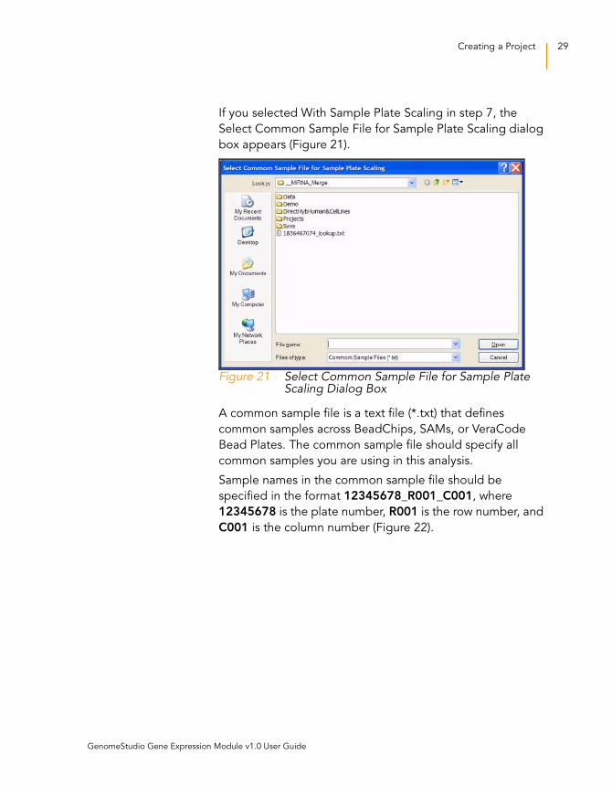
If you selected With Sample Plate Scaling in step 7, the
Select Common Sample File for Sample Plate Scaling dialog
box appears (Figure 21).
Figure 21 Select Common Sample File for Sample Plate Scaling Dialog Box
A common sample file is a text file (*.txt) that defines
common samples across BeadChips, SAMs, or VeraCode
Bead Plates. The common sample file should specify all
common samples you are using in this analysis.
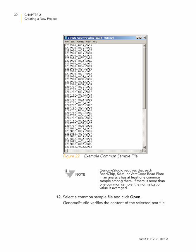
Sample names in the common sample file should be
specified in the format 12345678_R001_C001, where
12345678 is the plate number, R001 is the row number, and
C001 is the column number (Figure 22).
GenomeStudio Gene Expression Module v1.0 User Guide
30 CHAPTER 2
Creating a New Project
Figure 22 Example Common Sample File
12. Select a common sample file and click Open.
GenomeStudio verifies the content of the selected text file.
NOTE
GenomeStudio requires that each BeadChip, SAM, or VeraCode Bead Plate in an analysis has at least one common sample among them. If there is more than one common sample, the normalization value is averaged.
Part # 11319121 Rev. A
Creating a Project 31
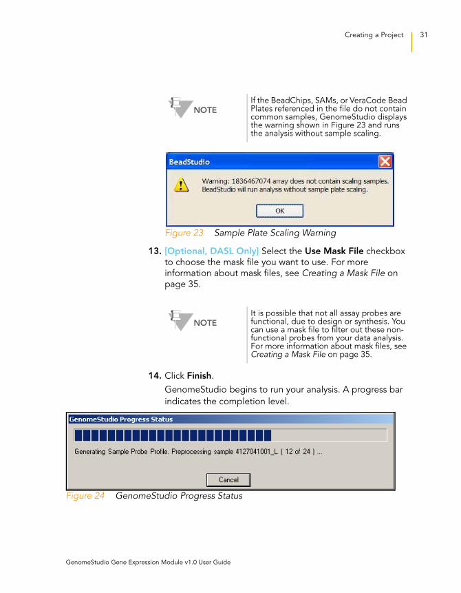
Figure 23 Sample Plate Scaling Warning
13. [Optional, DASL Only] Select the Use Mask File checkbox
to choose the mask file you want to use. For more
information about mask files, see Creating a Mask File on
page 35.
14. Click Finish.
GenomeStudio begins to run your analysis. A progress bar
indicates the completion level.
Figure 24 GenomeStudio Progress Status
NOTE
If the BeadChips, SAMs, or VeraCode Bead Plates referenced in the file do not contain common samples, GenomeStudio displays the warning shown in Figure 23 and runs the analysis without sample scaling.
NOTE
It is possible that not all assay probes are functional, due to design or synthesis. You can use a mask file to filter out these non-functional probes from your data analysis. For more information about mask files, see Creating a Mask File on page 35.
GenomeStudio Gene Expression Module v1.0 User Guide
32 CHAPTER 2
Creating a New Project
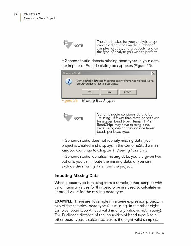
If GenomeStudio detects missing bead types in your data,
the Impute or Exclude dialog box appears (Figure 25).
Figure 25 Missing Bead Types
If GenomeStudio does not identify missing data, your
project is created and displays in the GenomeStudio main
window. Continue to Chapter 3, Viewing Your Data.
If GenomeStudio identifies missing data, you are given two
options: you can impute the missing data, or you can
exclude the missing data from the project.
Imputing Missing Data
When a bead type is missing from a sample, other samples with
valid intensity values for this bead type are used to calculate an
imputed value for the missing bead type.
EXAMPLE: There are 10 samples in a gene expression project. In
two of the samples, bead type A is missing. In the other eight
samples, bead type A has a valid intensity value (is not missing).
The Euclidean distance of the intensities of bead type A to all
other bead types is calculated across the eight valid samples.
NOTE
The time it takes for your analysis to be processed depends on the number of samples, groups, and groupsets, and on the type of analysis you wish to perform.
NOTE
GenomeStudio considers data to be “missing” if fewer than three beads exist for a given bead type. HumanHT-12 BeadChips may have missing data, because by design they include fewer beads per bead type.
Part # 11319121 Rev. A
Creating a Project 33
The goal is to find the bead types closest to bead type A from
the intensities of all valid samples. From these, the values of the
15 closest bead types are used to calculate the imputed value of
bead type A for the missing sample. The imputed value is
calculated as the weighted average of the 15 closest
probe intensities.
Bead standard error (BEAD_STDERR) is also imputed for the
missing bead type. This is calculated as the average of the bead
standard error values of this bead type for all valid samples.
The average number of beads (Avg_NBEADS) value is modified
in the data tables (e.g., Sample Probe Profile Table) to account
for the missing bead type. The number of beads is set to 1 for
the missing bead type in the data tables, but the actual number
of beads is shown in the Excluded and Imputed Probes Table.
Excluding Missing Data
You might decide to exclude missing data if you want to use only
raw data in your project. However, most of the time you will
probably want to impute missing data. Excluded data is removed
from GenomeStudio’s main tables, and moved to the Excluded
and Imputed Probes table.
15. [Missing Data Only] Do one of the following:
• If you would like to impute missing data,
click Yes.
• If you prefer to exclude missing data, click No.
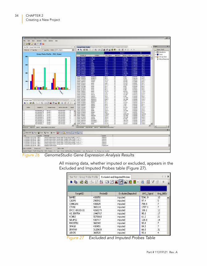
Your GenomeStudio Gene Expression project appears
(Figure 26).
NOTE
The Excluded and Imputed Probes table appears in a gene expression project only if the project contains imputed or excluded data. If there is no imputed or excluded data in a project, this table is not generated and does not appear.
GenomeStudio Gene Expression Module v1.0 User Guide
34 CHAPTER 2
Creating a New Project
Figure 26 GenomeStudio Gene Expression Analysis Results
All missing data, whether imputed or excluded, appears in the
Excluded and Imputed Probes table (Figure 27).
Figure 27 Excluded and Imputed Probes Table
Part # 11319121 Rev. A
Creating a Project 35
For more information about the Excluded and Imputed Probes
table and other elements of the Gene Expression Module
graphical user interface, see Chapter 7, User Interface Reference.
Creating aMask File
If genomic DNA was used in a DASL Assay to verify probe
performance, you can select probes that should be excluded
from further analysis. Because all probes are designed to be
intraexonic, all probes should be detectable when genomic DNA
is used as a sample. Therefore, the Detection p-value reported in
the Group Probe Profile Table or the Sample Probe Profile Table
can be used as an objective measure of probe performance on
genomic DNA.
Illumina recommends excluding probes that have a detection
p-value of greater than 0.01 on genomic DNA. However, you
may define your own exclusion criteria.
To exclude a probe:
1. Export the ProbeID, Detection Pval, and TargetID columns
from one of the Probe Profile Tables for the genomic DNA
samples to a text file.
2. Edit the text file so that all p-values above your detection
cutoff are set to 0, and all p-values below your detection
cutoff are set to 1.
For example, if you want to use a p-value cutoff of 0.01 for
detection, set all values above 0.01 to 0 and all values below
0.01 to 1.
3. Change the Detection Pval column header to “0/1” and save
the file as a *.csv file in the same repository where the
content descriptor file is stored. The file need not conform to
a naming convention.
NOTE
Any *.csv file present in the same repository as content descriptor files appears in the Experiment Parameters pulldown menu. To avoid confusion, Illumina recommends using separate repositories for content descriptor *.csv files and SAM/BeadChip/VeraCode Bead Plate data.
GenomeStudio Gene Expression Module v1.0 User Guide
36 CHAPTER 2
Creating a New Project
Applying aGroup Layout
File
GenomeStudio provides an optional alternative method for
creating large numbers of groups in complex experiments that
reduces project set-up time. The Apply Group Layout File
option allows you to apply a group layout file you previously
created in Excel (or a similar application) to a single SAM,
BeadChip, or VeraCode Bead Plate.
GenomeStudio creates groups according to the specifications in
the group layout file, and adds selected samples to those
groups.
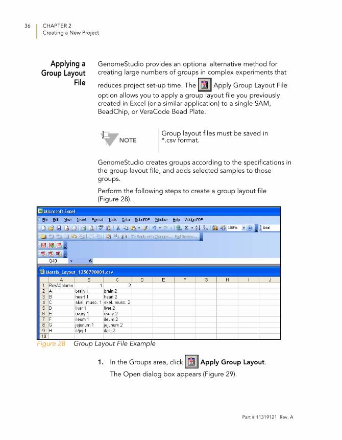
Perform the following steps to create a group layout file
(Figure 28).
Figure 28 Group Layout File Example
1. In the Groups area, click Apply Group Layout.
The Open dialog box appears (Figure 29).
NOTEGroup layout files must be saved in *.csv format.
Part # 11319121 Rev. A
Creating a Project 37
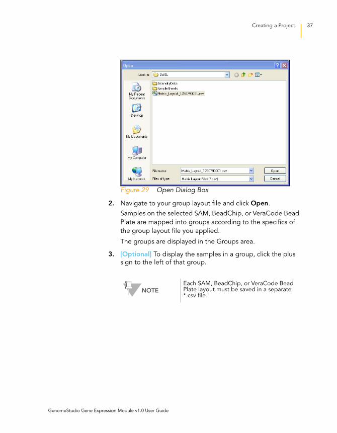
Figure 29 Open Dialog Box
2. Navigate to your group layout file and click Open.
Samples on the selected SAM, BeadChip, or VeraCode Bead
Plate are mapped into groups according to the specifics of
the group layout file you applied.
The groups are displayed in the Groups area.
3. [Optional] To display the samples in a group, click the plus
sign to the left of that group.
NOTE
Each SAM, BeadChip, or VeraCode Bead Plate layout must be saved in a separate *.csv file.
GenomeStudio Gene Expression Module v1.0 User Guide

38 CHAPTER 2
Creating a New Project
Part # 11319121 Rev. A

Chapter 3
Viewing Your Data
Topics40 Introduction
40 Scatter Plots
66 Bar Plots
69 Heat Maps
73 Cluster Analysis Dendrograms
81 Copy/Paste Clusters
85 Control Summary Reports
91 Image Viewer
GenomeStudio Gene Expression Module v1.0 User Guide
40 CHAPTER 3
Viewing Your Data
Introduction
This chapter describes the data visualization functions of the
GenomeStudio Gene Expression Module, which are used to
create and display:
Scatter plots
Bar plots
Line plots
Box plots
Heat maps
Cluster analysis dendrograms
Control summary reports
Histograms
Images
Use these tools to explore the data you create using the Gene
Analysis or Differential Expression Analysis tools (described in
Chapter 4, Normalization and Differential Analysis).
The Gene Expression Module also includes the Illumina Genome
Viewer (IGV), the Illumina Chromosome Browser (ICB), and the
Illumina Sequence Viewer (ISV). For more information about
these tools, see the GenomeStudio Framework User Guide,
Part # 11204578.
Scatter Plots
Once gene analysis and/or differential analysis have been
completed, you can create scatter plots.
To create a scatter plot:
1. Click Scatter Plot.
The Plot Columns dialog box appears (Figure 30).
Part # 11319121 Rev. A
Scatter Plots 41
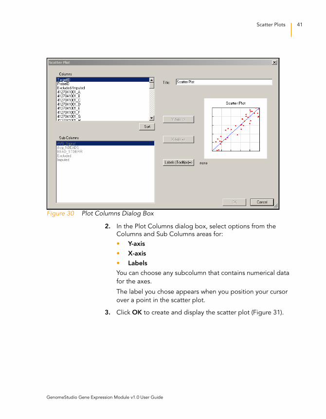
Figure 30 Plot Columns Dialog Box
2. In the Plot Columns dialog box, select options from the
Columns and Sub Columns areas for:
• Y-axis
• X-axis
• Labels
You can choose any subcolumn that contains numerical data
for the axes.
The label you chose appears when you position your cursor
over a point in the scatter plot.
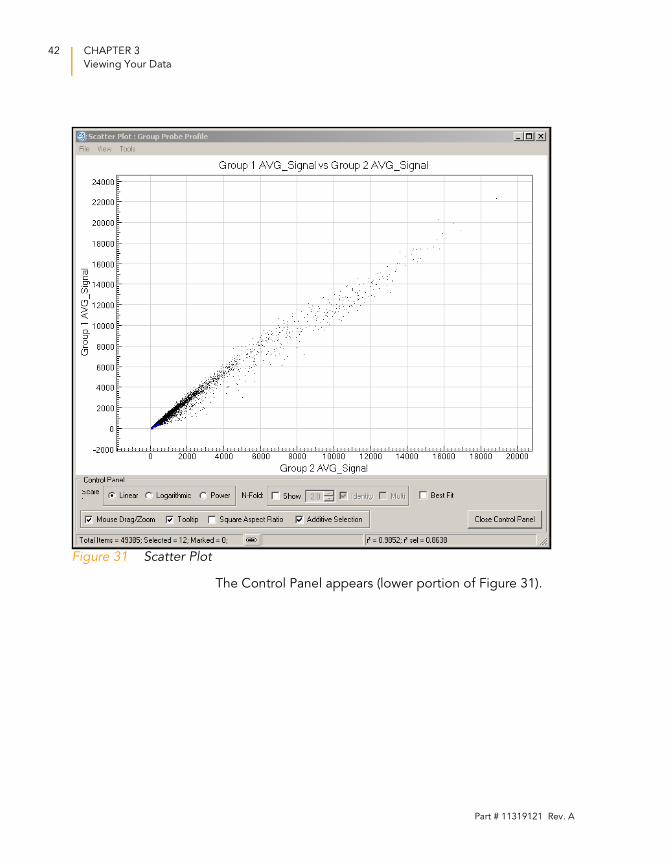
3. Click OK to create and display the scatter plot (Figure 31).
GenomeStudio Gene Expression Module v1.0 User Guide
42 CHAPTER 3
Viewing Your Data
Figure 31 Scatter Plot
The Control Panel appears (lower portion of Figure 31).
Part # 11319121 Rev. A
Scatter Plots 43
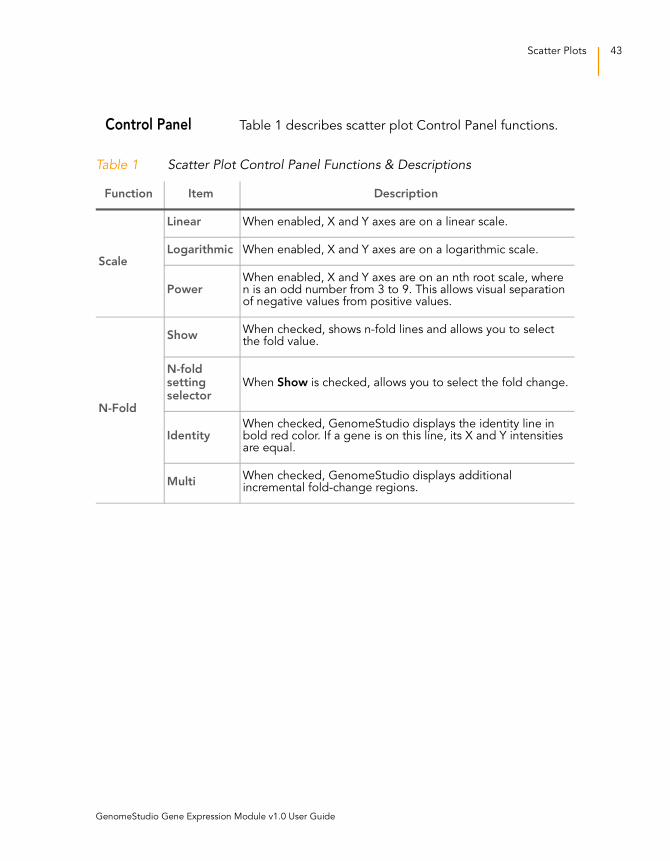
Control Panel Table 1 describes scatter plot Control Panel functions.
Table 1 Scatter Plot Control Panel Functions & Descriptions
Function Item Description
Scale
Linear When enabled, X and Y axes are on a linear scale.
Logarithmic When enabled, X and Y axes are on a logarithmic scale.
PowerWhen enabled, X and Y axes are on an nth root scale, where n is an odd number from 3 to 9. This allows visual separation of negative values from positive values.
N-Fold
ShowWhen checked, shows n-fold lines and allows you to select the fold value.
N-fold setting selector
When Show is checked, allows you to select the fold change.
IdentityWhen checked, GenomeStudio displays the identity line in bold red color. If a gene is on this line, its X and Y intensities are equal.
MultiWhen checked, GenomeStudio displays additional incremental fold-change regions.
GenomeStudio Gene Expression Module v1.0 User Guide
44 CHAPTER 3
Viewing Your Data
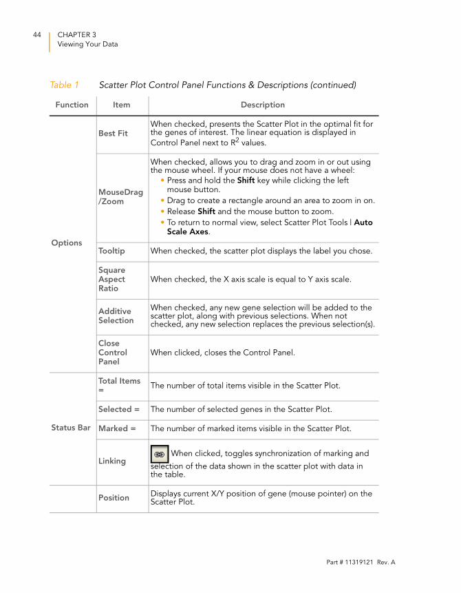
Options
Best FitWhen checked, presents the Scatter Plot in the optimal fit for the genes of interest. The linear equation is displayed in
Control Panel next to R2 values.
MouseDrag/Zoom
When checked, allows you to drag and zoom in or out using the mouse wheel. If your mouse does not have a wheel:
• Press and hold the Shift key while clicking the left mouse button.
• Drag to create a rectangle around an area to zoom in on.
• Release Shift and the mouse button to zoom.
• To return to normal view, select Scatter Plot Tools | Auto Scale Axes.
Tooltip When checked, the scatter plot displays the label you chose.
Square Aspect Ratio
When checked, the X axis scale is equal to Y axis scale.
Additive Selection
When checked, any new gene selection will be added to the scatter plot, along with previous selections. When not checked, any new selection replaces the previous selection(s).
Close Control Panel
When clicked, closes the Control Panel.
Status Bar
Total Items =
The number of total items visible in the Scatter Plot.
Selected = The number of selected genes in the Scatter Plot.
Marked = The number of marked items visible in the Scatter Plot.
Linking When clicked, toggles synchronization of marking and
selection of the data shown in the scatter plot with data in the table.
PositionDisplays current X/Y position of gene (mouse pointer) on the Scatter Plot.
Table 1 Scatter Plot Control Panel Functions & Descriptions (continued)
Function Item Description
Part # 11319121 Rev. A
Scatter Plots 45
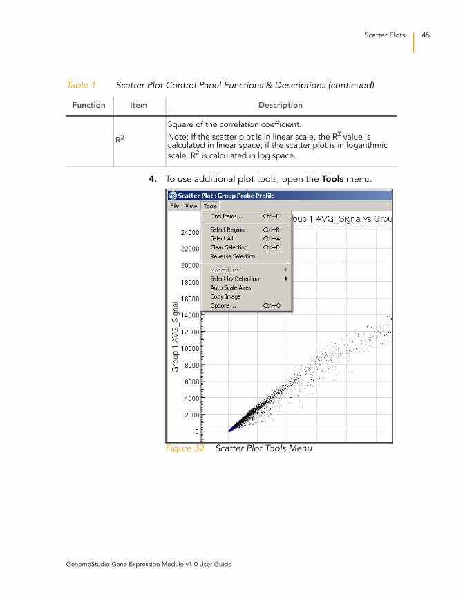
4. To use additional plot tools, open the Tools menu.
Figure 32 Scatter Plot Tools Menu
R2
Square of the correlation coefficient.
Note: If the scatter plot is in linear scale, the R2 value is calculated in linear space; if the scatter plot is in logarithmic
scale, R2 is calculated in log space.
Table 1 Scatter Plot Control Panel Functions & Descriptions (continued)
Function Item Description
GenomeStudio Gene Expression Module v1.0 User Guide
46 CHAPTER 3
Viewing Your Data
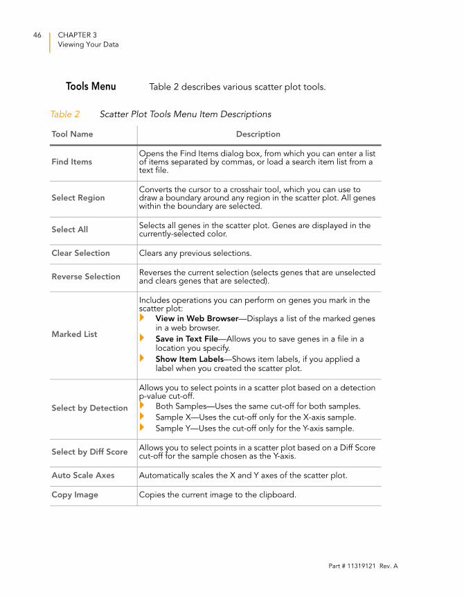
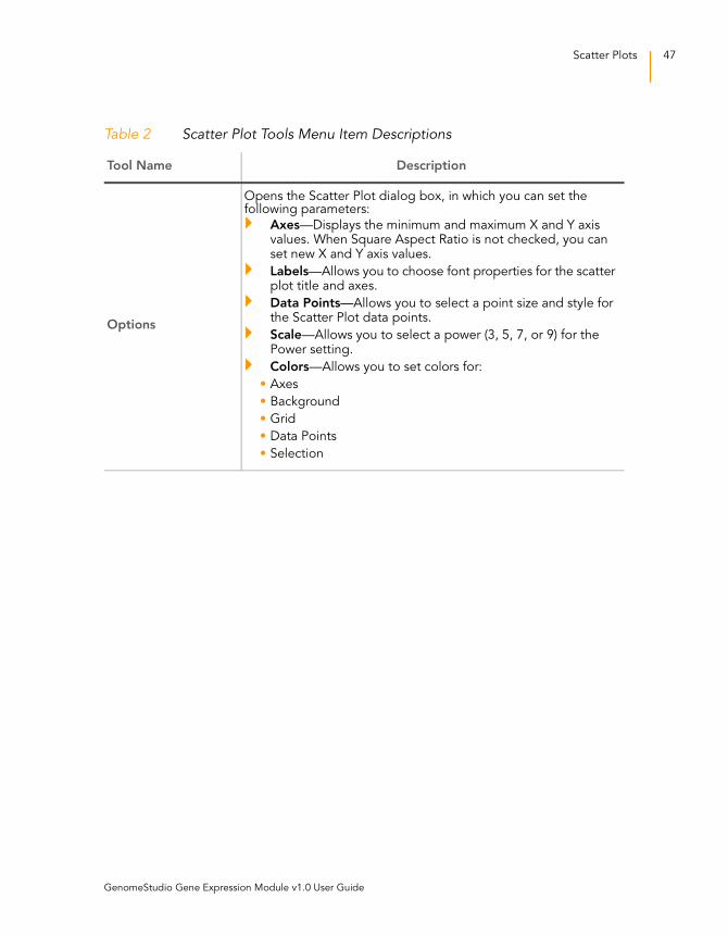
Tools Menu Table 2 describes various scatter plot tools.
Table 2 Scatter Plot Tools Menu Item Descriptions
Tool Name Description
Find ItemsOpens the Find Items dialog box, from which you can enter a list of items separated by commas, or load a search item list from a text file.
Select RegionConverts the cursor to a crosshair tool, which you can use to draw a boundary around any region in the scatter plot. All genes within the boundary are selected.
Select AllSelects all genes in the scatter plot. Genes are displayed in the currently-selected color.
Clear Selection Clears any previous selections.
Reverse SelectionReverses the current selection (selects genes that are unselected and clears genes that are selected).
Marked List
Includes operations you can perform on genes you mark in the scatter plot:
View in Web Browser—Displays a list of the marked genes in a web browser.
Save in Text File—Allows you to save genes in a file in a location you specify.
Show Item Labels—Shows item labels, if you applied a label when you created the scatter plot.
Select by Detection
Allows you to select points in a scatter plot based on a detection p-value cut-off.
Both Samples—Uses the same cut-off for both samples.
Sample X—Uses the cut-off only for the X-axis sample.
Sample Y—Uses the cut-off only for the Y-axis sample.
Select by Diff ScoreAllows you to select points in a scatter plot based on a Diff Score cut-off for the sample chosen as the Y-axis.
Auto Scale Axes Automatically scales the X and Y axes of the scatter plot.
Copy Image Copies the current image to the clipboard.
Part # 11319121 Rev. A
Scatter Plots 47
Options
Opens the Scatter Plot dialog box, in which you can set the following parameters:
Axes—Displays the minimum and maximum X and Y axis values. When Square Aspect Ratio is not checked, you can set new X and Y axis values.
Labels—Allows you to choose font properties for the scatter plot title and axes.
Data Points—Allows you to select a point size and style for the Scatter Plot data points.
Scale—Allows you to select a power (3, 5, 7, or 9) for the Power setting.
Colors—Allows you to set colors for:
• Axes
• Background
• Grid
• Data Points
• Selection
Table 2 Scatter Plot Tools Menu Item Descriptions
Tool Name Description
GenomeStudio Gene Expression Module v1.0 User Guide
48 CHAPTER 3
Viewing Your Data
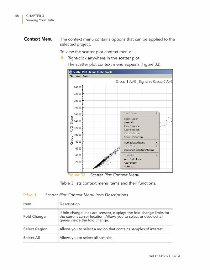
Context Menu The context menu contains options that can be applied to the
selected project.
To view the scatter plot context menu:
Right-click anywhere in the scatter plot.
The scatter plot context menu appears (Figure 33).
Figure 33 Scatter Plot Context Menu
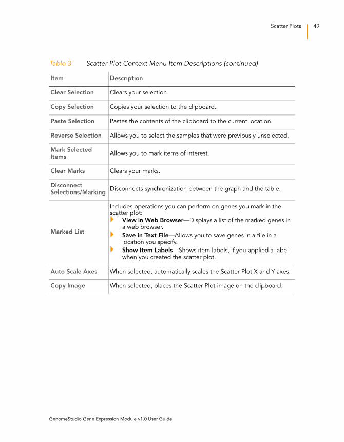
Table 3 lists context menu items and their functions.
Table 3 Scatter Plot Context Menu Item Descriptions
Item Description
Fold ChangeIf fold change lines are present, displays the fold change limits for the current cursor location. Allows you to select or deselect all genes inside the fold change.
Select Region Allows you to select a region that contains samples of interest.
Select All Allows you to select all samples.
Part # 11319121 Rev. A
Scatter Plots 49
Clear Selection Clears your selection.
Copy Selection Copies your selection to the clipboard.
Paste Selection Pastes the contents of the clipboard to the current location.
Reverse Selection Allows you to select the samples that were previously unselected.
Mark Selected Items
Allows you to mark items of interest.
Clear Marks Clears your marks.
Disconnect Selections/Marking
Disconnects synchronization between the graph and the table.
Marked List
Includes operations you can perform on genes you mark in the scatter plot:
View in Web Browser—Displays a list of the marked genes in a web browser.
Save in Text File—Allows you to save genes in a file in a location you specify.
Show Item Labels—Shows item labels, if you applied a label when you created the scatter plot.
Auto Scale Axes When selected, automatically scales the Scatter Plot X and Y axes.
Copy Image When selected, places the Scatter Plot image on the clipboard.
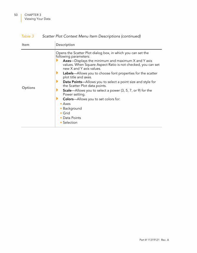
Table 3 Scatter Plot Context Menu Item Descriptions (continued)
Item Description
GenomeStudio Gene Expression Module v1.0 User Guide
50 CHAPTER 3
Viewing Your Data
Options
Opens the Scatter Plot dialog box, in which you can set the following parameters:
Axes—Displays the minimum and maximum X and Y axis values. When Square Aspect Ratio is not checked, you can set new X and Y axis values.
Labels—Allows you to choose font properties for the scatter plot title and axes.
Data Points—Allows you to select a point size and style for the Scatter Plot data points.
Scale—Allows you to select a power (3, 5, 7, or 9) for the Power setting.
Colors—Allows you to set colors for:
• Axes
• Background
• Grid
• Data Points
• Selection
Table 3 Scatter Plot Context Menu Item Descriptions (continued)
Item Description
Part # 11319121 Rev. A
Scatter Plots 51
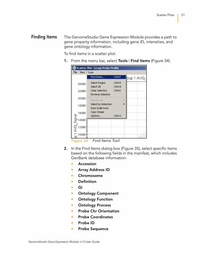
Finding Items The GenomeStudio Gene Expression Module provides a path to
gene property information, including gene ID, intensities, and
gene ontology information.
To find items in a scatter plot:
1. From the menu bar, select Tools | Find Items (Figure 34).
Figure 34 Find Items Tool
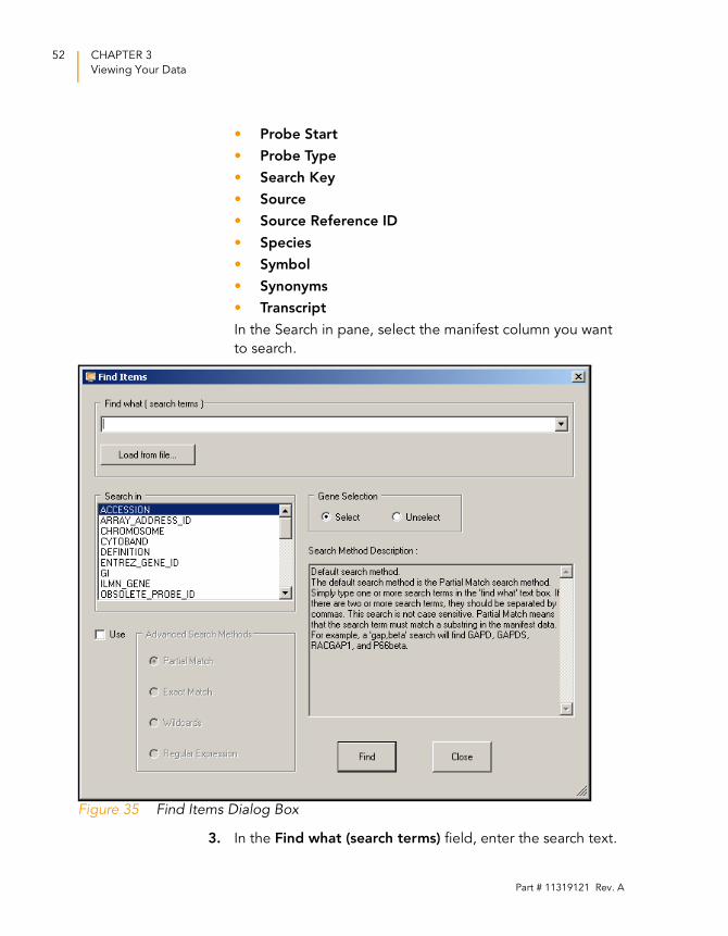
2. In the Find Items dialog box (Figure 35), select specific items
based on the following fields in the manifest, which includes
GenBank database information:
• Accession
• Array Address ID
• Chromosome
• Definition
• GI
• Ontology Component
• Ontology Function
• Ontology Process
• Probe Chr Orientation
• Probe Coordinates
• Probe ID
• Probe Sequence
GenomeStudio Gene Expression Module v1.0 User Guide
52 CHAPTER 3
Viewing Your Data
• Probe Start
• Probe Type
• Search Key
• Source
• Source Reference ID
• Species
• Symbol
• Synonyms
• Transcript
In the Search in pane, select the manifest column you want
to search.
Figure 35 Find Items Dialog Box
3. In the Find what (search terms) field, enter the search text.
Part # 11319121 Rev. A

Scatter Plots 53
4. Do one of the following:
• Click Select to select found genes.
• Click Unselect to clear found genes that were previously
selected.
5. Click Find to return to the scatter plot with the identified
genes highlighted.
For more advanced search options, click Use, to the left of
the Advanced Search Methods pane.
Advanced search methods are described in the Search
Method Description area (Figure 35).
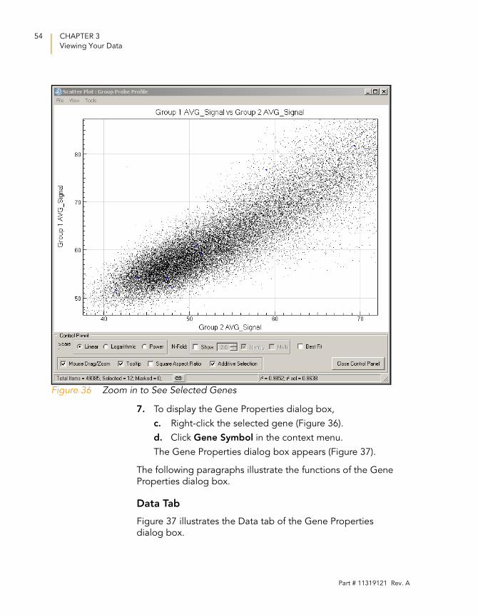
The scatter plot displays the selected gene (Figure 36).
6. [Optional] Use the mouse wheel to zoom in for a
magnified view.
NOTE
By default, searches are partial. For example, if you search the word 'VEGF' in the Symbol field, the search will return not only VEGF, but also VEGFB and VEGFC.
Multiple search terms can be used, separated by commas.
Search terms can also be loaded from a text file. The file should have each term on a separate line.
GenomeStudio Gene Expression Module v1.0 User Guide
54 CHAPTER 3
Viewing Your Data
Figure 36 Zoom in to See Selected Genes
7. To display the Gene Properties dialog box,
c. Right-click the selected gene (Figure 36).
d. Click Gene Symbol in the context menu.
The Gene Properties dialog box appears (Figure 37).
The following paragraphs illustrate the functions of the Gene
Properties dialog box.
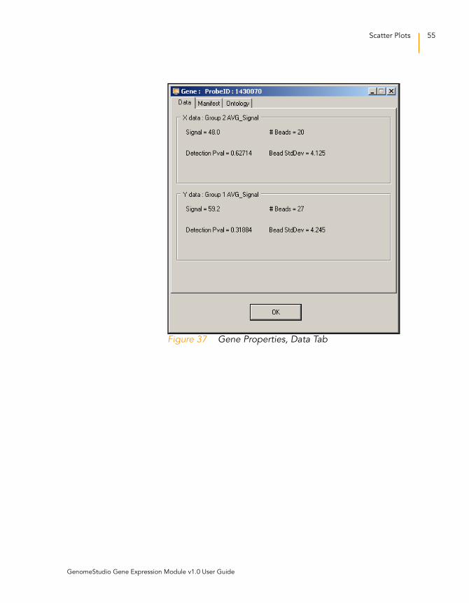
Data Tab
Figure 37 illustrates the Data tab of the Gene Properties
dialog box.
Part # 11319121 Rev. A
Scatter Plots 55
Figure 37 Gene Properties, Data Tab
GenomeStudio Gene Expression Module v1.0 User Guide
56 CHAPTER 3
Viewing Your Data
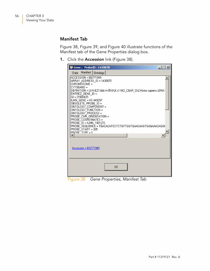
Manifest Tab
Figure 38, Figure 39, and Figure 40 illustrate functions of the
Manifest tab of the Gene Properties dialog box.
1. Click the Accession link (Figure 38).
Figure 38 Gene Properties, Manifest Tab
Part # 11319121 Rev. A
Scatter Plots 57
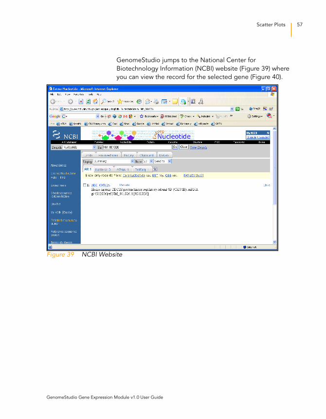
GenomeStudio jumps to the National Center for
Biotechnology Information (NCBI) website (Figure 39) where
you can view the record for the selected gene (Figure 40).
Figure 39 NCBI Website
GenomeStudio Gene Expression Module v1.0 User Guide
58 CHAPTER 3
Viewing Your Data
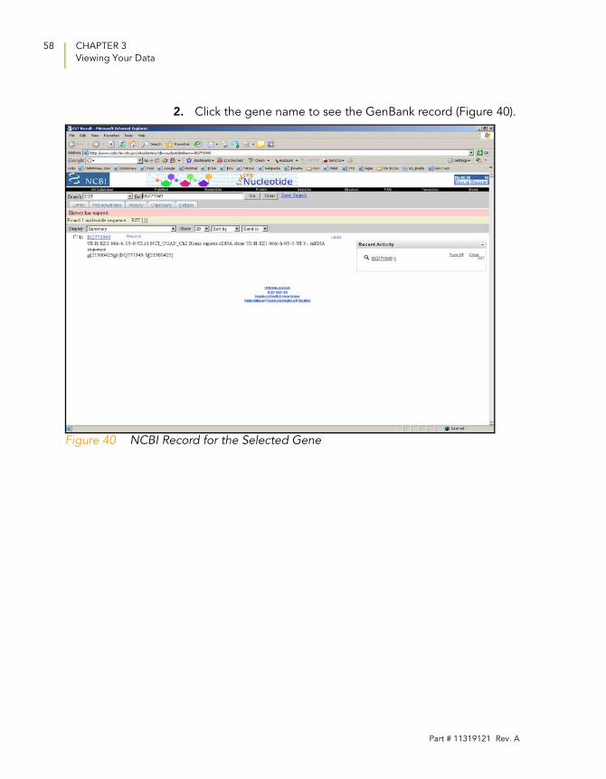
2. Click the gene name to see the GenBank record (Figure 40).
Figure 40 NCBI Record for the Selected Gene
Part # 11319121 Rev. A
Scatter Plots 59
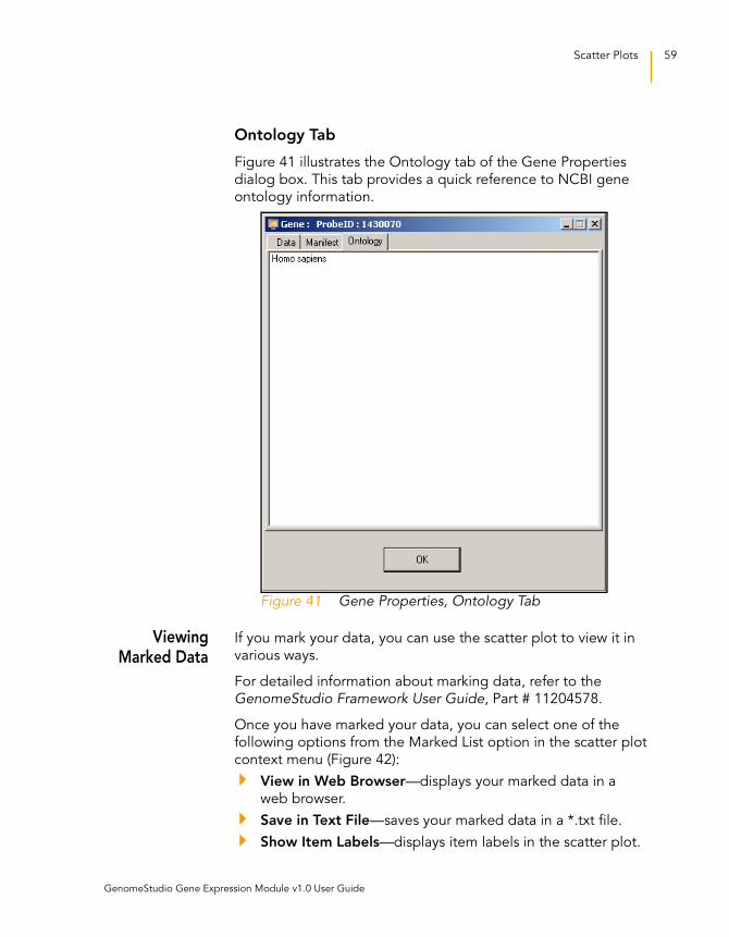
Ontology Tab
Figure 41 illustrates the Ontology tab of the Gene Properties
dialog box. This tab provides a quick reference to NCBI gene
ontology information.
Figure 41 Gene Properties, Ontology Tab
ViewingMarked Data
If you mark your data, you can use the scatter plot to view it in
various ways.
For detailed information about marking data, refer to the
GenomeStudio Framework User Guide, Part # 11204578.
Once you have marked your data, you can select one of the
following options from the Marked List option in the scatter plot
context menu (Figure 42):
View in Web Browser—displays your marked data in a
web browser.
Save in Text File—saves your marked data in a *.txt file.
Show Item Labels—displays item labels in the scatter plot.
GenomeStudio Gene Expression Module v1.0 User Guide
60 CHAPTER 3
Viewing Your Data
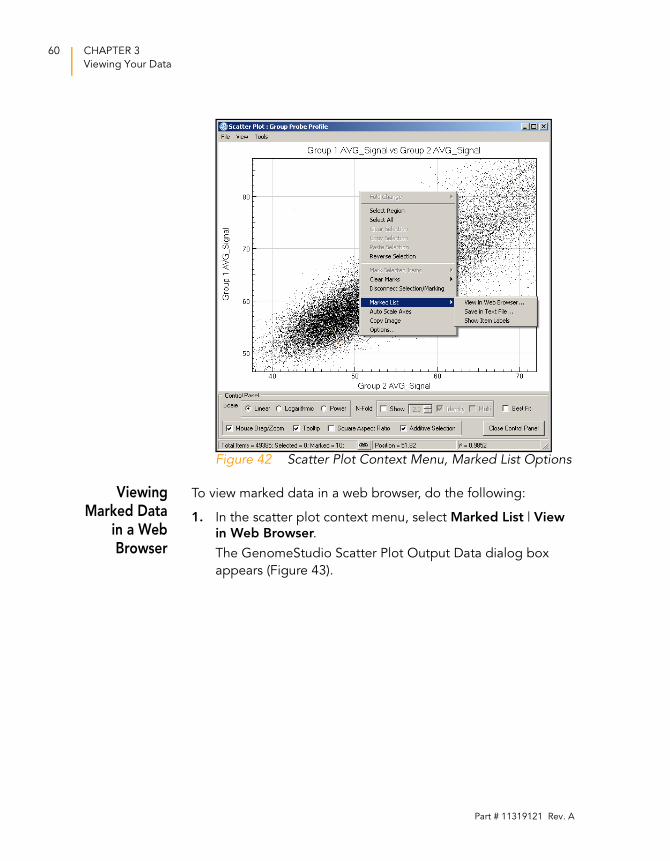
Figure 42 Scatter Plot Context Menu, Marked List Options
ViewingMarked Data
in a WebBrowser
To view marked data in a web browser, do the following:
1. In the scatter plot context menu, select Marked List | View
in Web Browser.
The GenomeStudio Scatter Plot Output Data dialog box
appears (Figure 43).
Part # 11319121 Rev. A
Scatter Plots 61
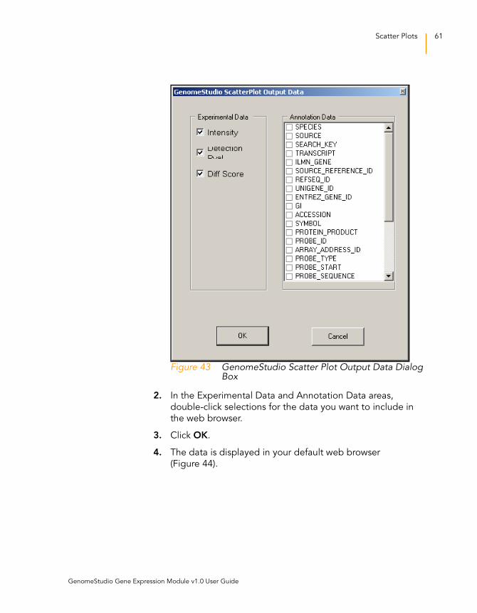
Figure 43 GenomeStudio Scatter Plot Output Data Dialog Box
2. In the Experimental Data and Annotation Data areas,
double-click selections for the data you want to include in
the web browser.
3. Click OK.
4. The data is displayed in your default web browser
(Figure 44).
GenomeStudio Gene Expression Module v1.0 User Guide
62 CHAPTER 3
Viewing Your Data
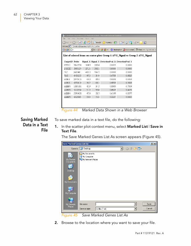
Figure 44 Marked Data Shown in a Web Browser
Saving MarkedData in a Text
File
To save marked data in a text file, do the following:
1. In the scatter plot context menu, select Marked List | Save in
Text File.
The Save Marked Genes List As screen appears (Figure 45).
Figure 45 Save Marked Genes List As
2. Browse to the location where you want to save your file.
Part # 11319121 Rev. A
Scatter Plots 63
3. Enter a name for your marked genes list in the File name
field.
4. Click Save.
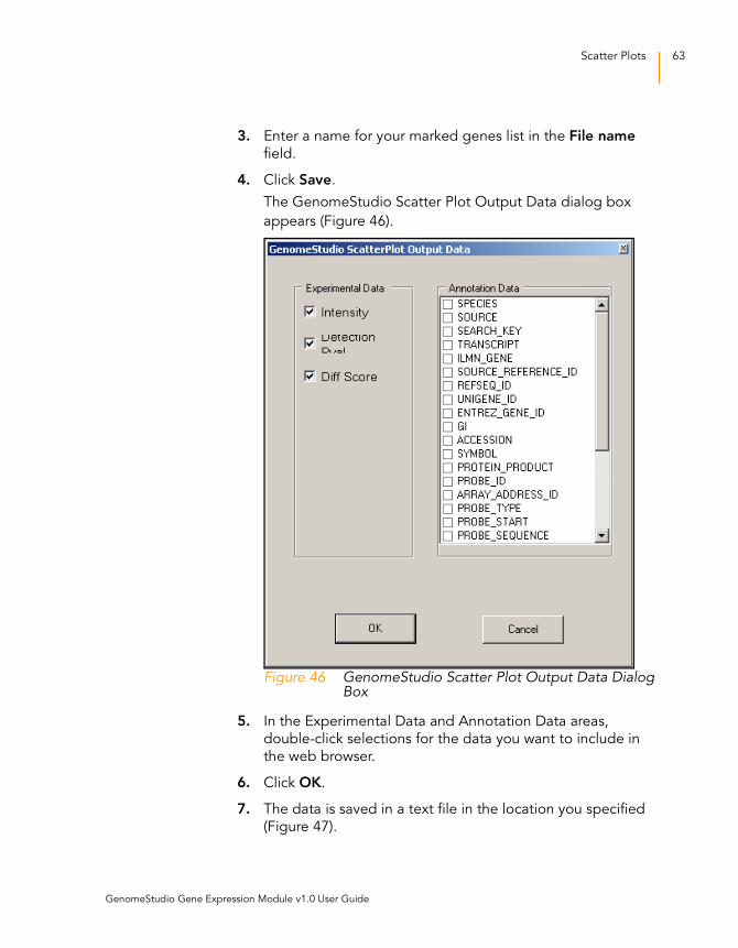
The GenomeStudio Scatter Plot Output Data dialog box
appears (Figure 46).
Figure 46 GenomeStudio Scatter Plot Output Data Dialog Box
5. In the Experimental Data and Annotation Data areas,
double-click selections for the data you want to include in
the web browser.
6. Click OK.
7. The data is saved in a text file in the location you specified
(Figure 47).
GenomeStudio Gene Expression Module v1.0 User Guide
64 CHAPTER 3
Viewing Your Data
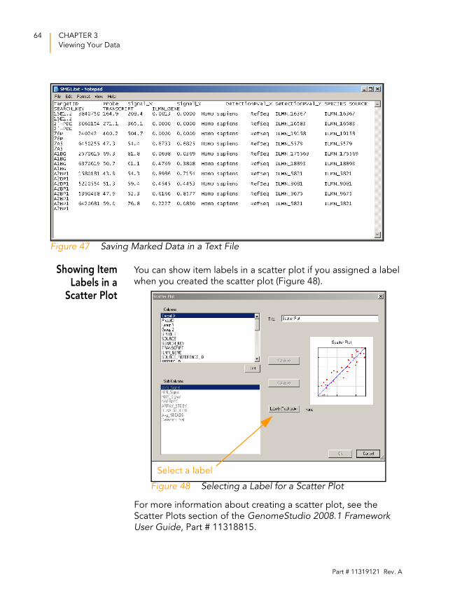
Figure 47 Saving Marked Data in a Text File
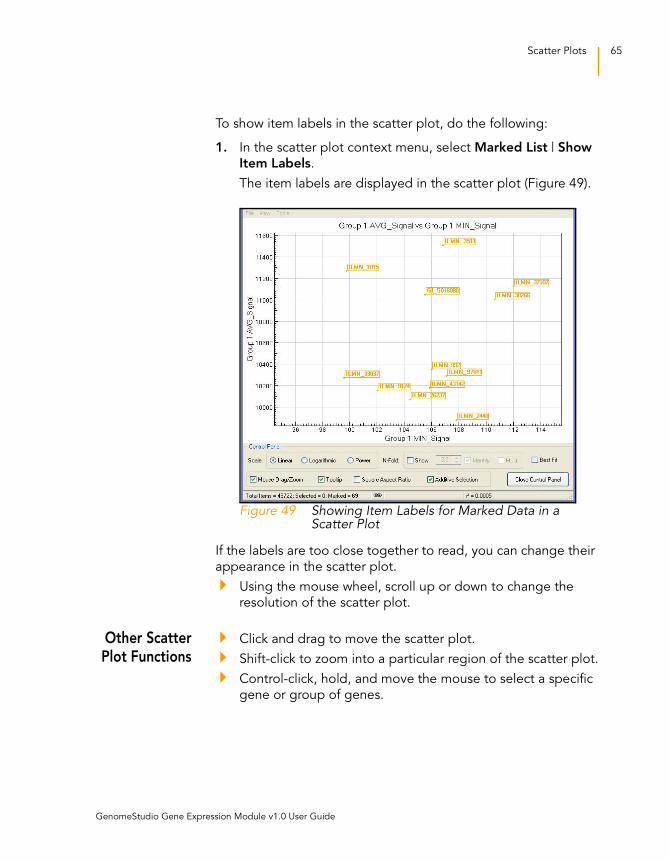
Showing ItemLabels in a
Scatter Plot
You can show item labels in a scatter plot if you assigned a label
when you created the scatter plot (Figure 48).
Figure 48 Selecting a Label for a Scatter Plot
For more information about creating a scatter plot, see the
Scatter Plots section of the GenomeStudio 2008.1 Framework User Guide, Part # 11318815.
Select a label
Part # 11319121 Rev. A
Scatter Plots 65
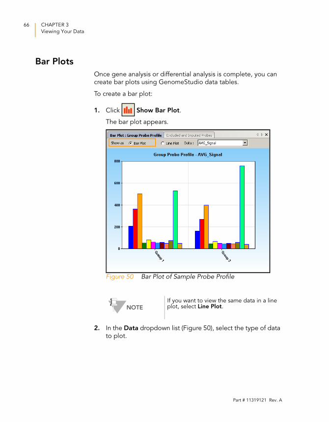
To show item labels in the scatter plot, do the following:
1. In the scatter plot context menu, select Marked List | Show
Item Labels.
The item labels are displayed in the scatter plot (Figure 49).
Figure 49 Showing Item Labels for Marked Data in a Scatter Plot
If the labels are too close together to read, you can change their
appearance in the scatter plot.
Using the mouse wheel, scroll up or down to change the
resolution of the scatter plot.
Other ScatterPlot Functions
Click and drag to move the scatter plot.
Shift-click to zoom into a particular region of the scatter plot.
Control-click, hold, and move the mouse to select a specific
gene or group of genes.
GenomeStudio Gene Expression Module v1.0 User Guide
66 CHAPTER 3
Viewing Your Data
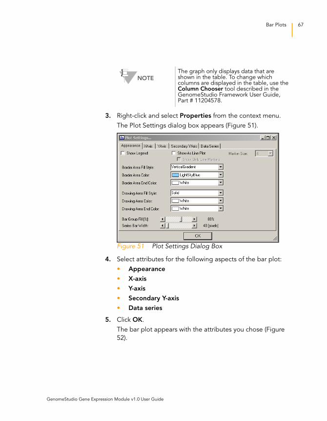
Bar Plots
Once gene analysis or differential analysis is complete, you can
create bar plots using GenomeStudio data tables.
To create a bar plot:
1. Click Show Bar Plot.
The bar plot appears.
Figure 50 Bar Plot of Sample Probe Profile
2. In the Data dropdown list (Figure 50), select the type of data
to plot.
NOTE
If you want to view the same data in a line plot, select Line Plot.
Part # 11319121 Rev. A
Bar Plots 67
3. Right-click and select Properties from the context menu.
The Plot Settings dialog box appears (Figure 51).
Figure 51 Plot Settings Dialog Box
4. Select attributes for the following aspects of the bar plot:
• Appearance
• X-axis
• Y-axis
• Secondary Y-axis
• Data series
5. Click OK.
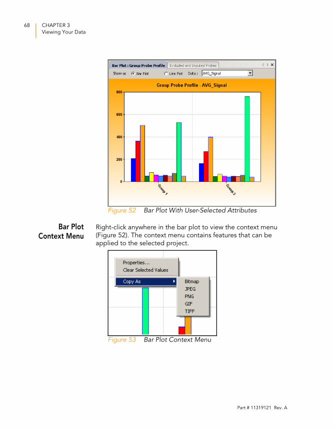
The bar plot appears with the attributes you chose (Figure
52).
NOTE
The graph only displays data that are shown in the table. To change which columns are displayed in the table, use the Column Chooser tool described in the GenomeStudio Framework User Guide, Part # 11204578.
GenomeStudio Gene Expression Module v1.0 User Guide
68 CHAPTER 3
Viewing Your Data
Figure 52 Bar Plot With User-Selected Attributes
Bar PlotContext Menu
Right-click anywhere in the bar plot to view the context menu
(Figure 52). The context menu contains features that can be
applied to the selected project.
Figure 53 Bar Plot Context Menu
Part # 11319121 Rev. A
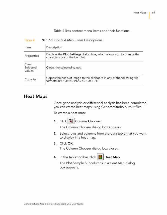
Heat Maps 69
Table 4 lists context menu items and their functions.
Heat Maps
Once gene analysis or differential analysis has been completed,
you can create heat maps using GenomeStudio output files.
To create a heat map:
1. Click Column Chooser.
The Column Chooser dialog box appears.
2. Select rows and columns from the data table that you want
to display in a heat map.
3. Click OK.
The Column Chooser dialog box closes.
4. In the table toolbar, click Heat Map.
The Plot Sample Subcolumns in a Heat Map dialog
box appears.
Table 4 Bar Plot Context Menu Item Descriptions
Item Description
PropertiesDisplays the Plot Settings dialog box, which allows you to change the characteristics of the bar plot.
Clear Selected Values
Clears the selected values.
Copy AsCopies the bar plot image to the clipboard in any of the following file formats: BMP, JPEG, PNG, GIF, or TIFF.
GenomeStudio Gene Expression Module v1.0 User Guide
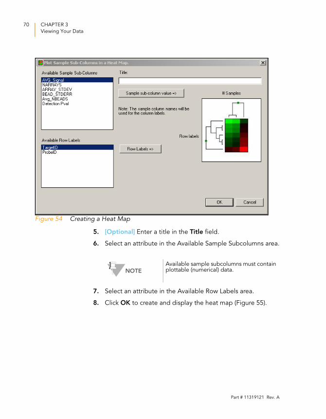
70 CHAPTER 3
Viewing Your Data
Figure 54 Creating a Heat Map
5. [Optional] Enter a title in the Title field.
6. Select an attribute in the Available Sample Subcolumns area.
7. Select an attribute in the Available Row Labels area.
8. Click OK to create and display the heat map (Figure 55).
NOTE
Available sample subcolumns must contain plottable (numerical) data.
Part # 11319121 Rev. A
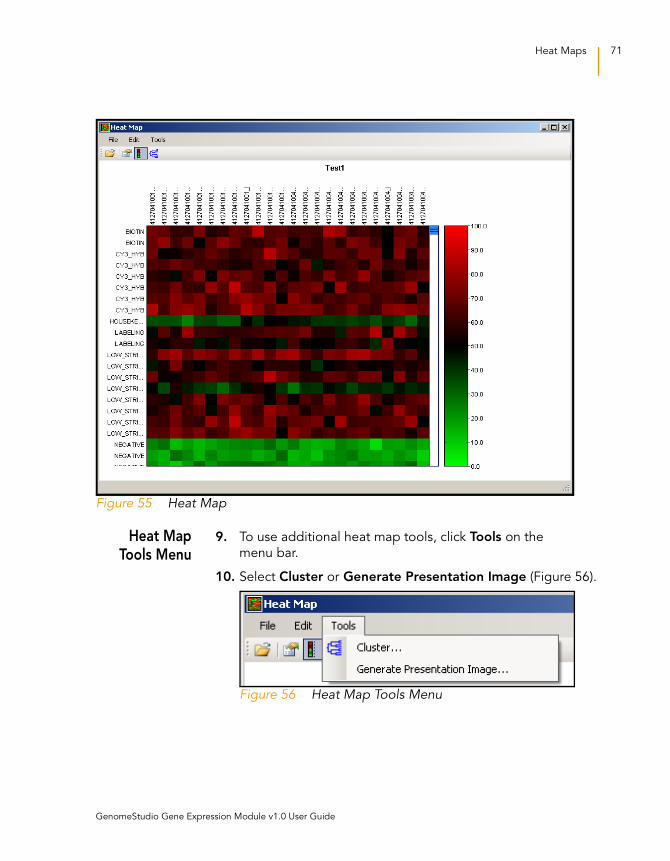
Heat Maps 71
Figure 55 Heat Map
Heat MapTools Menu
9. To use additional heat map tools, click Tools on the
menu bar.
10. Select Cluster or Generate Presentation Image (Figure 56).
Figure 56 Heat Map Tools Menu
GenomeStudio Gene Expression Module v1.0 User Guide
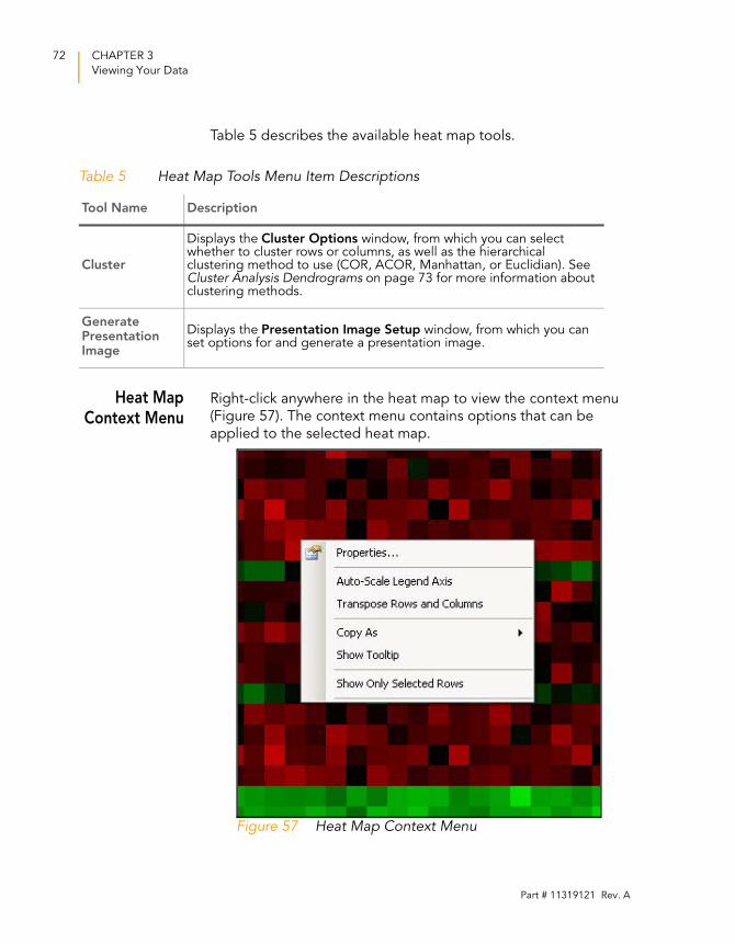
72 CHAPTER 3
Viewing Your Data
Table 5 describes the available heat map tools.
Heat MapContext Menu
Right-click anywhere in the heat map to view the context menu
(Figure 57). The context menu contains options that can be
applied to the selected heat map.
Figure 57 Heat Map Context Menu
Table 5 Heat Map Tools Menu Item Descriptions
Tool Name Description
Cluster
Displays the Cluster Options window, from which you can select whether to cluster rows or columns, as well as the hierarchical clustering method to use (COR, ACOR, Manhattan, or Euclidian). See Cluster Analysis Dendrograms on page 73 for more information about clustering methods.
Generate Presentation Image
Displays the Presentation Image Setup window, from which you can set options for and generate a presentation image.
Part # 11319121 Rev. A
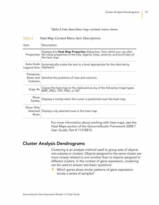
Cluster Analysis Dendrograms 73
Table 6 lists describes map context menu items.
For more information about working with heat maps, see the
Heat Maps section of the GenomeStudio Framework 2008.1 User Guide, Part # 11318815.
Cluster Analysis Dendrograms
Clustering is an analysis method used to group sets of objects
into subsets or clusters. Objects assigned to the same cluster are
more closely related to one another than to objects assigned to
different clusters. In the context of gene expression, clustering
can be used to answer two basic questions:
Which genes show similar patterns of gene expression
across a series of samples?
Table 6 Heat Map Context Menu Item Descriptions
Item Description
PropertiesDisplays the Heat Map Properties dialog box, from which you can alter the visual properties of the title, legend, rows, columns, and scroll bars of the heat map.
Auto-Scale
Legend AxisAutomatically scales the axis to a level appropriate for the data being displayed.
Transpose
Rows and
Columns
Switches the positions of rows and columns.
Copy AsCopies the heat map to the clipboard as any of the following image types: BMP, JPEG, TIFF, PNG, or GIF.
Show
TooltipDisplays a tooltip when the cursor is positioned over the heat map.
Show Only
Selected
Rows
Displays only selected rows in the heat map.
GenomeStudio Gene Expression Module v1.0 User Guide
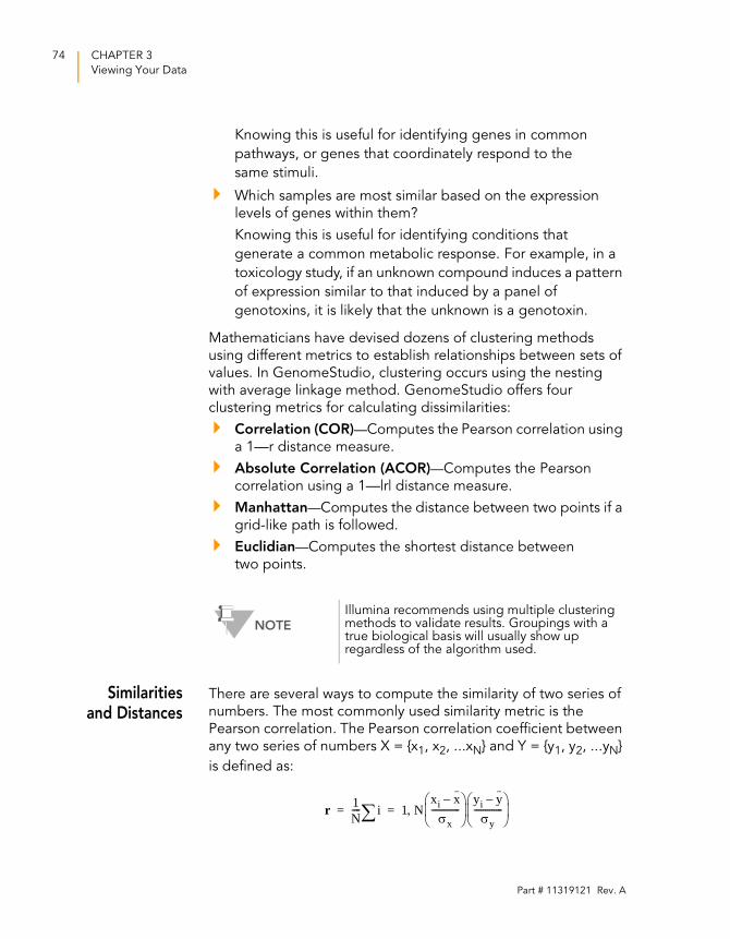
74 CHAPTER 3
Viewing Your Data
Knowing this is useful for identifying genes in common
pathways, or genes that coordinately respond to the
same stimuli.
Which samples are most similar based on the expression
levels of genes within them?
Knowing this is useful for identifying conditions that
generate a common metabolic response. For example, in a
toxicology study, if an unknown compound induces a pattern
of expression similar to that induced by a panel of
genotoxins, it is likely that the unknown is a genotoxin.
Mathematicians have devised dozens of clustering methods
using different metrics to establish relationships between sets of
values. In GenomeStudio, clustering occurs using the nesting
with average linkage method. GenomeStudio offers four
clustering metrics for calculating dissimilarities:
Correlation (COR)—Computes the Pearson correlation using
a 1—r distance measure.
Absolute Correlation (ACOR)—Computes the Pearson
correlation using a 1—|r| distance measure.
Manhattan—Computes the distance between two points if a
grid-like path is followed.
Euclidian—Computes the shortest distance between
two points.
Similaritiesand Distances
There are several ways to compute the similarity of two series of
numbers. The most commonly used similarity metric is the
Pearson correlation. The Pearson correlation coefficient between
any two series of numbers X = {x1, x2, ...xN} and Y = {y1, y2, ...yN}
is defined as:
NOTE
Illumina recommends using multiple clustering methods to validate results. Groupings with a true biological basis will usually show up regardless of the algorithm used.
r 1N---- i∑ 1 N
xi x–σx
-------------⎝ ⎠⎜ ⎟⎛ ⎞ yi y–
σy-------------⎝ ⎠⎜ ⎟⎛ ⎞
,= =
Part # 11319121 Rev. A
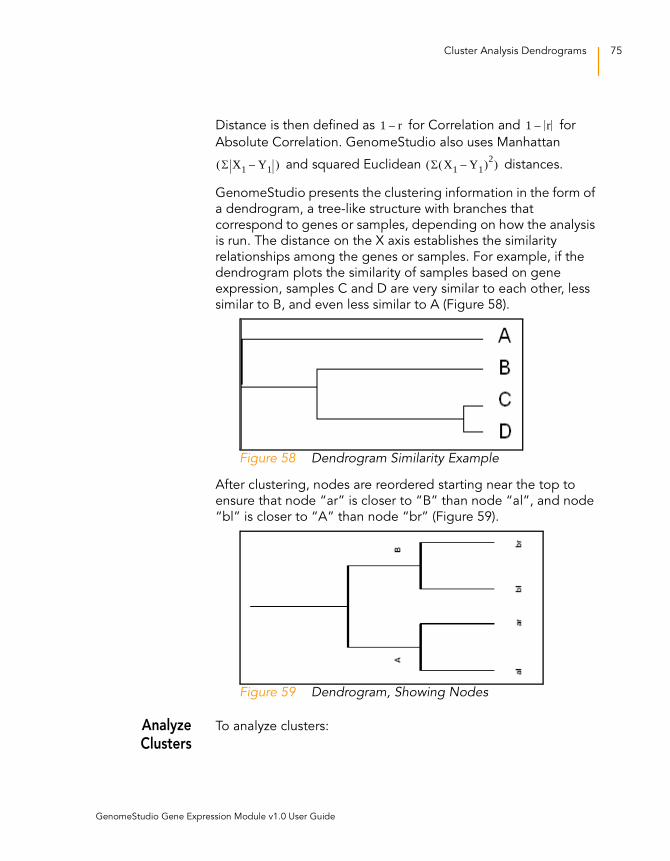
Cluster Analysis Dendrograms 75
Distance is then defined as for Correlation and for
Absolute Correlation. GenomeStudio also uses Manhattan
and squared Euclidean distances.
GenomeStudio presents the clustering information in the form of
a dendrogram, a tree-like structure with branches that
correspond to genes or samples, depending on how the analysis
is run. The distance on the X axis establishes the similarity
relationships among the genes or samples. For example, if the
dendrogram plots the similarity of samples based on gene
expression, samples C and D are very similar to each other, less
similar to B, and even less similar to A (Figure 58).
Figure 58 Dendrogram Similarity Example
After clustering, nodes are reordered starting near the top to
ensure that node “ar” is closer to “B” than node “al”, and node
“bl” is closer to “A” than node “br” (Figure 59).
Figure 59 Dendrogram, Showing Nodes
AnalyzeClusters
To analyze clusters:
1 r– 1 r–
Σ X1 Y1–( ) Σ X1 Y1–( )2( )
GenomeStudio Gene Expression Module v1.0 User Guide
76 CHAPTER 3
Viewing Your Data
1. Click Run Cluster Analysis to open the cluster
analysis tool.
2. In the Cluster Analysis dialog box (Figure 60), perform the
following steps:
a. Groups pane—Highlight the group(s) whose clusters you
wish to analyze. Select the Sort checkbox to sort the
items in the Groups listbox alphabetically in
ascending order.
b. Cluster pane—Click Genes or Samples.
If you select Genes, the dendrogram displays a cluster
of genes.
If you select Samples, the dendrogram displays a cluster
of samples.
c. Metric pane—Select the metric you would like
GenomeStudio to use to calculate clusters.
NOTE
Clustering samples is much faster than clustering genes. Clustering thousands of genes can take hours.
Part # 11319121 Rev. A
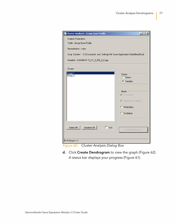
Cluster Analysis Dendrograms 77
Figure 60 Cluster Analysis Dialog Box
d. Click Create Dendrogram to view the graph (Figure 62).
A status bar displays your progress (Figure 61).
GenomeStudio Gene Expression Module v1.0 User Guide
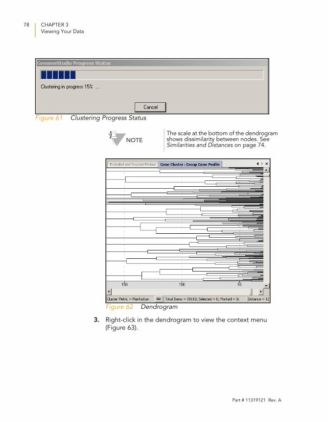
78 CHAPTER 3
Viewing Your Data
Figure 61 Clustering Progress Status
Figure 62 Dendrogram
3. Right-click in the dendrogram to view the context menu
(Figure 63).
NOTE
The scale at the bottom of the dendrogram shows dissimilarity between nodes. See Similarities and Distances on page 74.
Part # 11319121 Rev. A
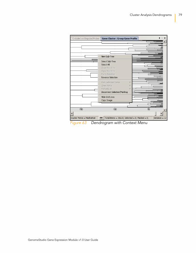
Cluster Analysis Dendrograms 79
Figure 63 Dendrogram with Context Menu
GenomeStudio Gene Expression Module v1.0 User Guide
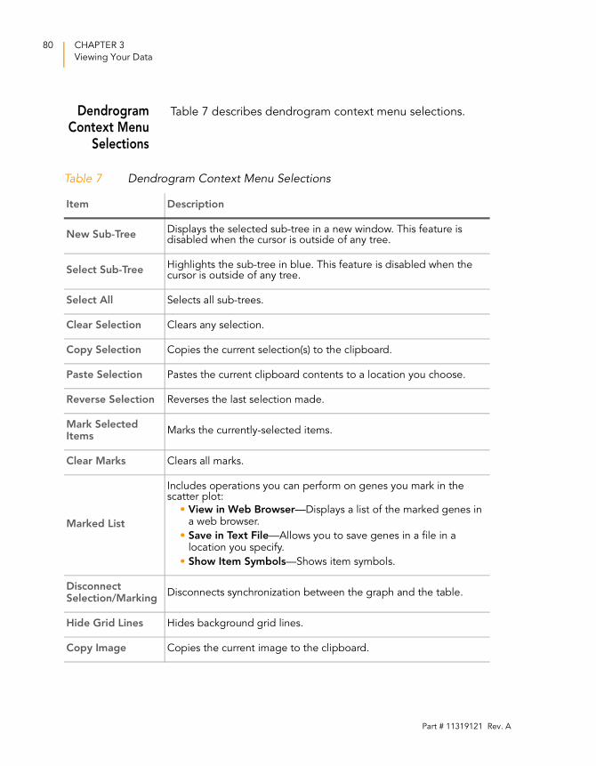
80 CHAPTER 3
Viewing Your Data
DendrogramContext Menu
Selections
Table 7 describes dendrogram context menu selections.
Table 7 Dendrogram Context Menu Selections
Item Description
New Sub-TreeDisplays the selected sub-tree in a new window. This feature is disabled when the cursor is outside of any tree.
Select Sub-TreeHighlights the sub-tree in blue. This feature is disabled when the cursor is outside of any tree.
Select All Selects all sub-trees.
Clear Selection Clears any selection.
Copy Selection Copies the current selection(s) to the clipboard.
Paste Selection Pastes the current clipboard contents to a location you choose.
Reverse Selection Reverses the last selection made.
Mark Selected Items
Marks the currently-selected items.
Clear Marks Clears all marks.
Marked List
Includes operations you can perform on genes you mark in the scatter plot:
• View in Web Browser—Displays a list of the marked genes in a web browser.
• Save in Text File—Allows you to save genes in a file in a location you specify.
• Show Item Symbols—Shows item symbols.
Disconnect Selection/Marking
Disconnects synchronization between the graph and the table.
Hide Grid Lines Hides background grid lines.
Copy Image Copies the current image to the clipboard.
Part # 11319121 Rev. A
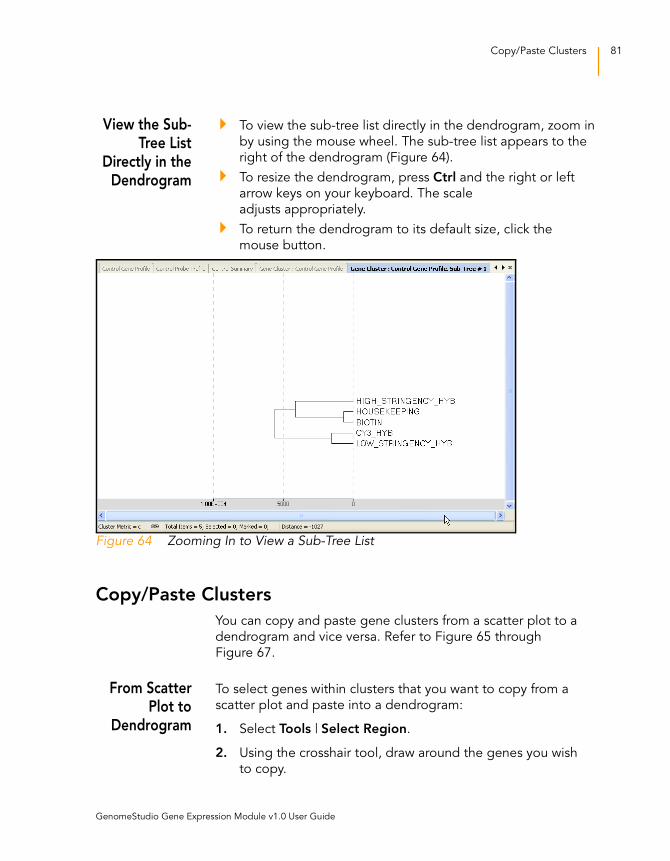
Copy/Paste Clusters 81
View the Sub-Tree List
Directly in theDendrogram
To view the sub-tree list directly in the dendrogram, zoom in
by using the mouse wheel. The sub-tree list appears to the
right of the dendrogram (Figure 64).
To resize the dendrogram, press Ctrl and the right or left
arrow keys on your keyboard. The scale
adjusts appropriately.
To return the dendrogram to its default size, click the
mouse button.
Figure 64 Zooming In to View a Sub-Tree List
Copy/Paste Clusters
You can copy and paste gene clusters from a scatter plot to a
dendrogram and vice versa. Refer to Figure 65 through
Figure 67.
From ScatterPlot to
Dendrogram
To select genes within clusters that you want to copy from a
scatter plot and paste into a dendrogram:
1. Select Tools | Select Region.
2. Using the crosshair tool, draw around the genes you wish
to copy.
GenomeStudio Gene Expression Module v1.0 User Guide
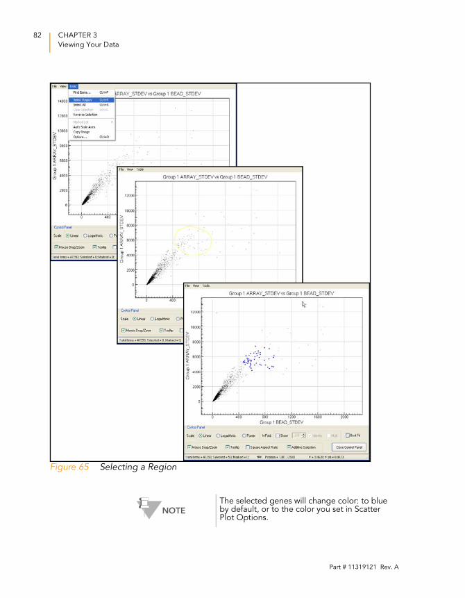
82 CHAPTER 3
Viewing Your Data
Figure 65 Selecting a Region
NOTE
The selected genes will change color: to blue by default, or to the color you set in Scatter Plot Options.
Part # 11319121 Rev. A

Copy/Paste Clusters 83
3. To copy the selection to the clipboard, select Tools |
Copy Selection.
4. To paste the selection into the dendrogram, select Tools |
Paste Selection.
FromDendrogram
to Scatter Plot
To select clusters for copying from the dendrogram:
1. Position the cursor over the sub-tree you want to copy.
2. Right-click and click Select Sub-Tree from the context menu.
NOTE
Click inside the sub-tree you want to select. The sub-tree you select appears in blue.
GenomeStudio Gene Expression Module v1.0 User Guide
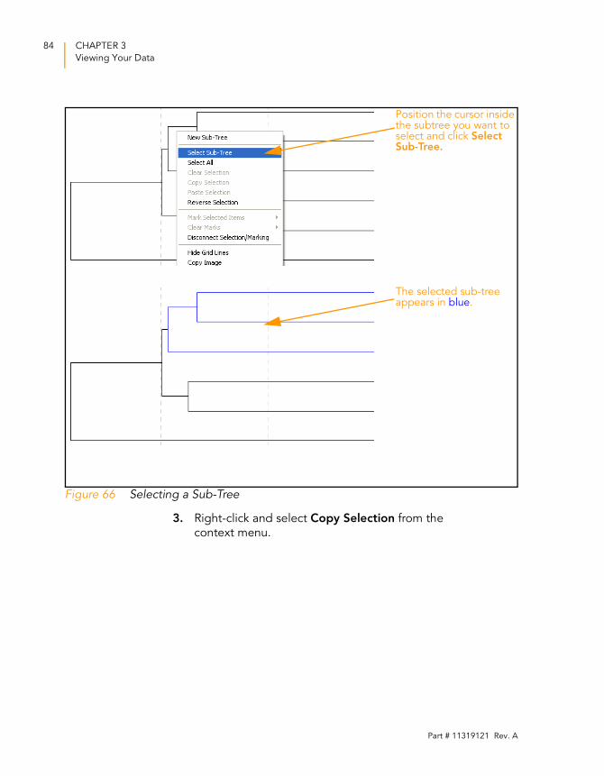
84 CHAPTER 3
Viewing Your Data
Figure 66 Selecting a Sub-Tree
3. Right-click and select Copy Selection from the
context menu.
Position the cursor inside the subtree you want to select and click Select Sub-Tree.
The selected sub-tree appears in blue.
Part # 11319121 Rev. A
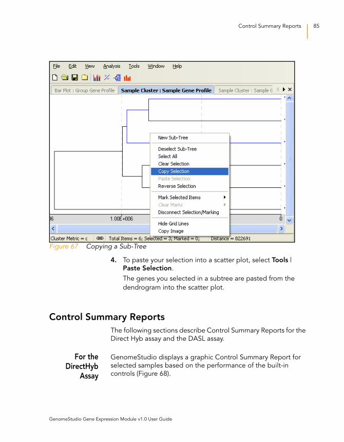
Control Summary Reports 85
Figure 67 Copying a Sub-Tree
4. To paste your selection into a scatter plot, select Tools |
Paste Selection.
The genes you selected in a subtree are pasted from the
dendrogram into the scatter plot.
Control Summary Reports
The following sections describe Control Summary Reports for the
Direct Hyb assay and the DASL assay.
For theDirectHyb
Assay
GenomeStudio displays a graphic Control Summary Report for
selected samples based on the performance of the built-in
controls (Figure 68).
GenomeStudio Gene Expression Module v1.0 User Guide
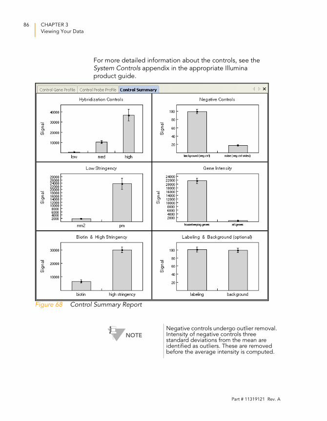
86 CHAPTER 3
Viewing Your Data
For more detailed information about the controls, see the
System Controls appendix in the appropriate Illumina
product guide.
Figure 68 Control Summary Report
NOTE
Negative controls undergo outlier removal. Intensity of negative controls three standard deviations from the mean are identified as outliers. These are removed before the average intensity is computed.
Part # 11319121 Rev. A

Control Summary Reports 87
5. To view secondary graph(s), click on a data point at the top
of a bar in any of the graphs shown in Figure 68. Each point
in the secondary graph represents a sample.
Figure 69 Housekeeping Controls Secondary Graph
6. To copy, change the page setup, or see a print preview,
right click in any graph to use the context menu.
7. To print the graph, click Print in the menu bar (Figure 70).
GenomeStudio Gene Expression Module v1.0 User Guide
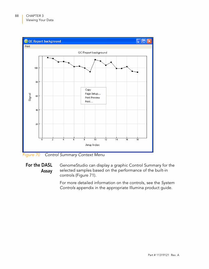
88 CHAPTER 3
Viewing Your Data
Figure 70 Control Summary Context Menu
For the DASLAssay
GenomeStudio can display a graphic Control Summary for the
selected samples based on the performance of the built-in
controls (Figure 71).
For more detailed information on the controls, see the System Controls appendix in the appropriate Illumina product guide.
Part # 11319121 Rev. A
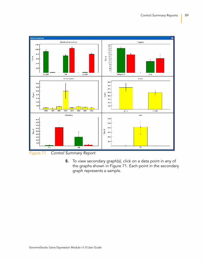
Control Summary Reports 89
Figure 71 Control Summary Report
8. To view secondary graph(s), click on a data point in any of
the graphs shown in Figure 71. Each point in the secondary
graph represents a sample.
GenomeStudio Gene Expression Module v1.0 User Guide
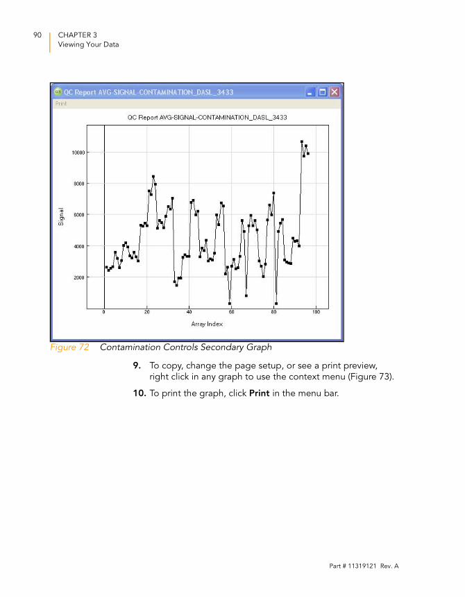
90 CHAPTER 3
Viewing Your Data
Figure 72 Contamination Controls Secondary Graph
9. To copy, change the page setup, or see a print preview,
right click in any graph to use the context menu (Figure 73).
10. To print the graph, click Print in the menu bar.
Part # 11319121 Rev. A
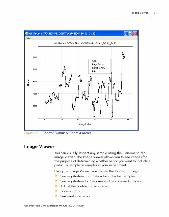
Image Viewer 91
Figure 73 Control Summary Context Menu
Image Viewer
You can visually inspect any sample using the GenomeStudio
Image Viewer. The Image Viewer allows you to see images for
the purpose of determining whether or not you want to include a
particular sample or samples in your experiment.
Using the Image Viewer, you can do the following things:
See registration information for individual samples
See registration for GenomeStudio-processed images
Adjust the contrast of an image
Zoom in or out
See pixel intensities
GenomeStudio Gene Expression Module v1.0 User Guide
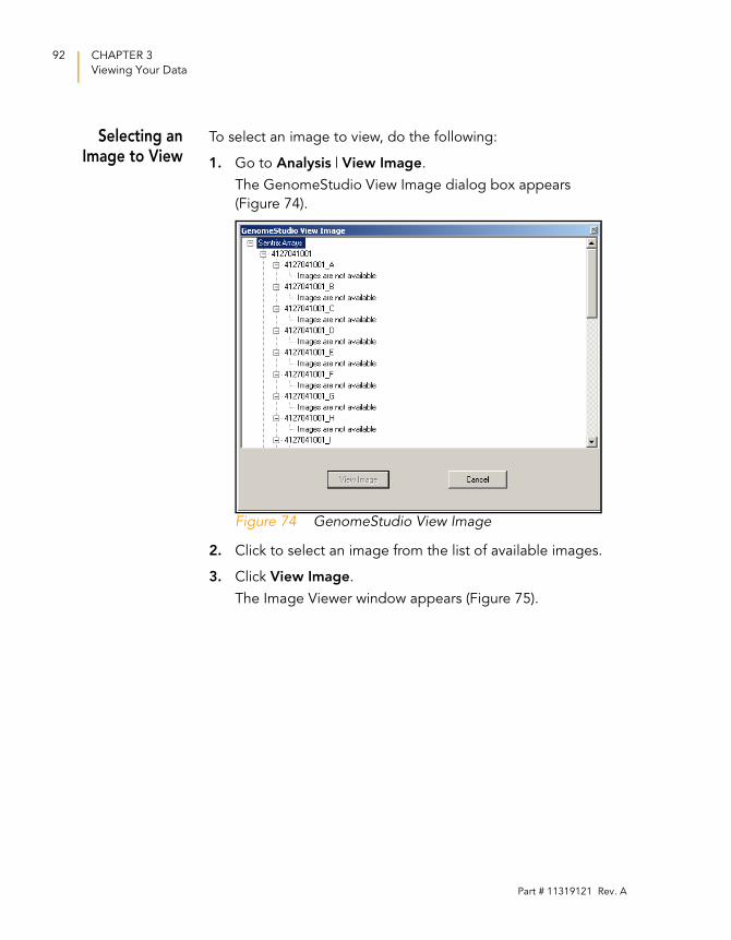
92 CHAPTER 3
Viewing Your Data
Selecting anImage to View
To select an image to view, do the following:
1. Go to Analysis | View Image.
The GenomeStudio View Image dialog box appears
(Figure 74).
Figure 74 GenomeStudio View Image
2. Click to select an image from the list of available images.
3. Click View Image.
The Image Viewer window appears (Figure 75).
Part # 11319121 Rev. A
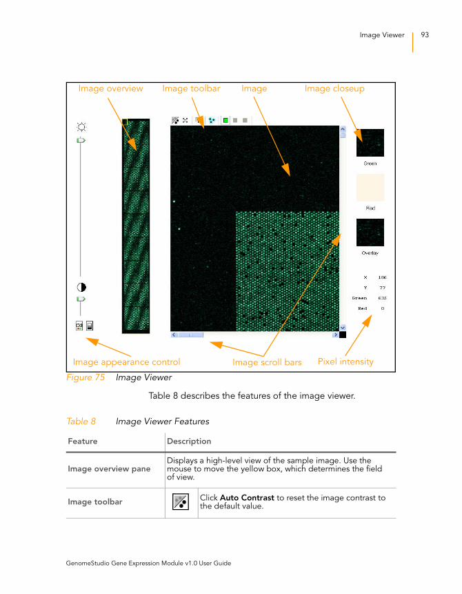
Image Viewer 93
Figure 75 Image Viewer
Table 8 describes the features of the image viewer.
Image scroll bars
Image closeupImage overview Image Image toolbar
Pixel intensityImage appearance control
Table 8 Image Viewer Features
Feature Description
Image overview paneDisplays a high-level view of the sample image. Use the mouse to move the yellow box, which determines the field of view.
Image toolbarClick Auto Contrast to reset the image contrast to the default value.
GenomeStudio Gene Expression Module v1.0 User Guide
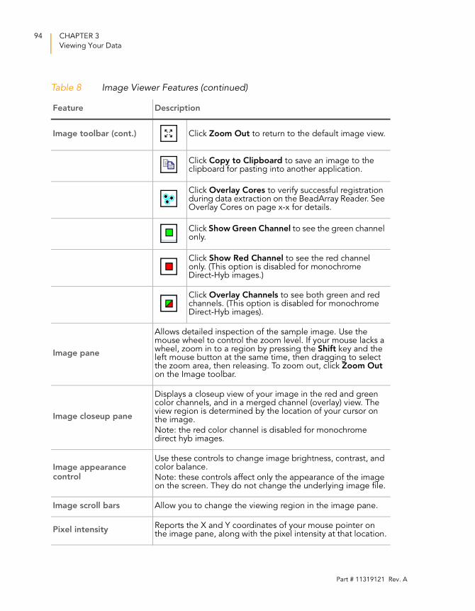
94 CHAPTER 3
Viewing Your Data
Image toolbar (cont.) Click Zoom Out to return to the default image view.
Click Copy to Clipboard to save an image to the clipboard for pasting into another application.
Click Overlay Cores to verify successful registration during data extraction on the BeadArray Reader. See Overlay Cores on page x-x for details.
Click Show Green Channel to see the green channel only.
Click Show Red Channel to see the red channel only. (This option is disabled for monochrome Direct-Hyb images.)
Click Overlay Channels to see both green and red channels. (This option is disabled for monochrome Direct-Hyb images).
Image pane
Allows detailed inspection of the sample image. Use the mouse wheel to control the zoom level. If your mouse lacks a wheel, zoom in to a region by pressing the Shift key and the left mouse button at the same time, then dragging to select the zoom area, then releasing. To zoom out, click Zoom Out on the Image toolbar.
Image closeup pane
Displays a closeup view of your image in the red and green color channels, and in a merged channel (overlay) view. The view region is determined by the location of your cursor on the image.
Note: the red color channel is disabled for monochrome direct hyb images.
Image appearance control
Use these controls to change image brightness, contrast, and color balance.
Note: these controls affect only the appearance of the image on the screen. They do not change the underlying image file.
Image scroll bars Allow you to change the viewing region in the image pane.
Pixel intensityReports the X and Y coordinates of your mouse pointer on the image pane, along with the pixel intensity at that location.
Table 8 Image Viewer Features (continued)
Feature Description
Part # 11319121 Rev. A
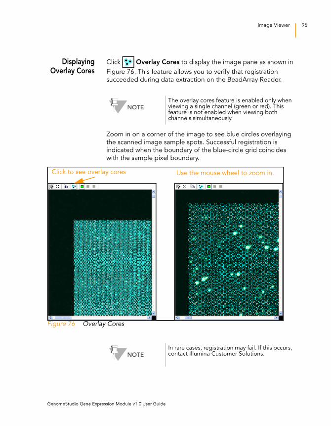
Image Viewer 95
DisplayingOverlay Cores
Click Overlay Cores to display the image pane as shown in
Figure 76. This feature allows you to verify that registration
succeeded during data extraction on the BeadArray Reader.
Zoom in on a corner of the image to see blue circles overlaying
the scanned image sample spots. Successful registration is
indicated when the boundary of the blue-circle grid coincides
with the sample pixel boundary.
Figure 76 Overlay Cores
NOTE
The overlay cores feature is enabled only when viewing a single channel (green or red). This feature is not enabled when viewing both channels simultaneously.
Click to see overlay cores Use the mouse wheel to zoom in.
NOTE
In rare cases, registration may fail. If this occurs, contact Illumina Customer Solutions.
GenomeStudio Gene Expression Module v1.0 User Guide
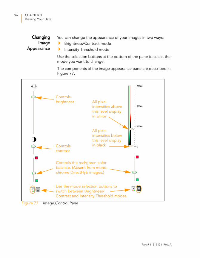
96 CHAPTER 3
Viewing Your Data
ChangingImage
Appearance
You can change the appearance of your images in two ways:
Brightness/Contract mode
Intensity Threshold mode
Use the selection buttons at the bottom of the pane to select the
mode you want to change.
The components of the image appearance pane are described in
Figure 77.
Figure 77 Image Control Pane
Controls
Controls
All pixel
intensities above
this level display
in white
All pixel
intensities below
this level display
in black
Use the mode selection buttons to
switch between Brightness/
Contrast and Intensity Threshold modes.
brightness
contrast
Controls the red/green color
balance. (Absent from mono-
chrome DirectHyb images.)
Part # 11319121 Rev. A

Chapter 4
Normalization and
Differential Analysis
Topics98 Introduction
98 Normalization Methods & Algorithms
99 Sample Scaling
99 Average
100 Quantile
101 Cubic Spline
102 Rank Invariant
103 Differential Expression Algorithms
103 Illumina Custom
105 Mann-Whitney
105 T-Test
106 Detection P-Value
106 Whole Genome BeadChips
107 DASL, miRNA, VeraCode DASL, and Focused Arrays
GenomeStudio Gene Expression Module v1.0 User Guide
98 CHAPTER 4
Normalization and Differential Analysis
Introduction
This chapter describes the statistical algorithms used in
GenomeStudio gene expression analysis.
Normalization Methods & Algorithms
Normalization algorithms adjust sample signals in order to
minimize the effects of variation arising from non-biological
factors. The GenomeStudio Gene Expression Module offers
several routines that are described in the following sections.
For all algorithms, normalization is computed with respect to a
mathematically calculated “virtual” sample that represents
averaged probe intensities across a group of samples.
In the case of cubic spline or rank invariant normalization, the
virtual sample is computed differently for SAMs than it is
for BeadChips:
For SAMs, the virtual sample is computed based on the
content of the reference group. If there is no reference
group, the first group displayed in the Project Group pane is
used for group analysis.
For BeadChips, the virtual sample is computed based on the
average of all samples in the experiment.
For quantile normalization, all samples are used to calculate the
virtual array. Group information is not used.
The following sections contain detailed description of these
normalization algorithms:
Average
Sample scaling
Quantile
Cubic spline
Rank invariant
Part # 11319121 Rev. A
Normalization Methods & Algorithms 99
Sample Scaling Sample scaling normalization is applied when technical
replicates are present in the sample set. This is a scaling
normalization that is performed on a per-probe basis.
Let i range from 1 to the number of probes, let j range from 1 to
the number of replicates, let m range from 1 to the number of
samples, and let equal the intensity for any given probe.
For the case where only one replicate is present between two
SAMs or BeadChips, a scaling factor ( ) is computed as follows:
where j = 1, 2.
For multiple replicates, the per-probe intensities are averaged
before computing the scaling factor.
Next, each probe for each sample is normalized as follows:
See Figure 22 in Chapter 2.
Average Sample intensities are scaled by a factor equal to the ratio of
average intensity of virtual sample to the average intensity of the
given sample. Background is subtracted prior to the scaling.
Average normalization adjusts for differences in overall intensity
between arrays and chips. Sample intensities are scaled by a
factor so that the average signal of all samples becomes equal to
the global average of all sample signals. Background subtraction
is done prior to scaling, so half of the unexpressed targets are
expected to have negative signals.
I
sfi
sfiIi1Ii2------=
Iimnorm sfi Iim( )=
NOTE
When you use a sample sheet, the Sample_Name in the Common Samples File must match the Sample_Name in the sample sheet.
If no sample sheet is used, the common sample names must be in the form Sentrix Barcode Number_Array Position.e.g., 12345678_R000_C000.
GenomeStudio Gene Expression Module v1.0 User Guide

100 CHAPTER 4
Normalization and Differential Analysis
Quantile Quantile normalization is a method used to make the
distribution, median, and mean of probe intensities the same for
every sample. The normalization distribution is chosen by
averaging each quantile across samples. Like cubic spline, this
method assumes that all samples have similar distributions of
transcript abundance.
The quantile normalization algorithm works as follows:
1. Given n samples with p probes, form X from the dimensions
p x n where each sample is a column and each probe is
a row.
2. Sort each column of X to get Xs.
3. Take the means across rows of Xs.
4. Assign this mean to each element in a row to get Xsm.
5. Get Xnormalized by rearranging each column of Xsm to have
the same ordering as the original X.
6. Xnormalized now contains the normalized intensity for all
samples (columns) and all probes (rows).
NOTE
Negative control probes are normalized together with analytical probes.
NOTE
Quantile is not recommended if you have titration samples in your project. In this case, Illumina recommends average normalization.
Part # 11319121 Rev. A
Normalization Methods & Algorithms 101
Cubic Spline Cubic spline normalization is similar to the method proposed by
Workman et al.1 The normalization uses quantiles of sample
intensities to fit smoothing B-splines.
Let
be a vector of N quantiles
Here, is the number of probes represented on a sample.
For each sample, the vector of quantile intensities is computed.
Similarly, quantiles for the “virtual” averaged sample after
background subtraction are computed. Cubic B-spline is
computed and used for interpolation. For points with intensities
ranked outside the interval, linear extrapolation rather than cubic
spline is used to avoid nonlinear effects outside the region
of interpolation.
1. Workman C, Jensen LJ, Jarmer H, Berka R, Gautier L, Nielser HB, Saxild HH, Nielsen C, Brunak S, Knudsen S. A new non-linear normalization method for reducing variability in DNA microarray experiments. Genome Biol. 2002 Aug 30; 3(9):research0048. PMID: 12225587 [PubMed - indexed for MEDLINE]
Cubic spline normalization is capable of minimizing effects that
cause nonlinear transformation of data, such as saturation. This is
similar to the method proposed by Workman et. al. Just as in the
rank invariant method, cubic spline normalization is computed
with respect to the virtual reference sample. The assumption of
this method is that all samples have similar distributions of
transcript abundance. The transformation is computed using
smoothing B-splines. The number of quantiles equals 1% of the
number of probes, but cannot be lower than 15. For points
outside of the interpolation interval, linear extrapolation is used.
This method is applied after the background normalization
method described above.
NOTE
For the DASL assay, red and green channels are normalized independently.
qii 0.5–
N--------------- i, 1 2…N,= =
N max 15Nprobes
100------------------,⎝ ⎠
⎛ ⎞=⎝ ⎠⎛ ⎞
Nprobes
GenomeStudio Gene Expression Module v1.0 User Guide
102 CHAPTER 4
Normalization and Differential Analysis
Rank Invariant Rank invariant normalization uses a set of probes that is rank
invariant between a given sample and a virtual sample.
The rank invariant set is found as follows: we start by considering
probes with intensities ranked between LowRank = 50th
percentile and HighRank = 90th percentile. If the probe’s
relative rank changes the probe is considered to be
rank invariant. If less than 2% of all probes in the region are
identified as rank invariant, LowRank is gradually decreased until
it reaches the 25th percentile.
Rank invariant normalization operates under the assumption that
probes with similar ranking between samples have similar
expression levels. This method minimizes the effects of additive
and multiplicative factors. The subset of probes with low relative
rank change is defined as follows.
1. The virtual reference sample is created by averaging the
content of the reference group (in differential analysis) or the
first group of the group set (in gene analysis).
2. All probes ranked between LowRank = 50th and HighRank =
90th percentiles are considered. If the change of rank relative
to the virtual reference is less than 0.05, the probe is
considered to be “rank invariant.”
3. If less than 2% of all probes are picked as rank invariant,
LowRank is gradually decreased until it reaches the 25th
percentile.
4. Normalization coefficients are computed using iteratively re-
weighted least squares. This method is applied after the
background normalization method described above.
rx rv–rv
--------------- 0.05≤
Part # 11319121 Rev. A
Differential Expression Algorithms 103
Differential Expression Algorithms
All algorithms compare a group of samples (referred to as the
condition group) to a reference group. The comparison is done
using the following error models:
Illumina Custom
Mann-Whitney
T-Test
IlluminaCustom
This model assumes that target signal intensity (I) is normally
distributed among replicates corresponding to some biological
condition. The variation has three components: sequence
specific biological variation , nonspecific biological
variation , and technical error .
= a + b < I >
Variation of nonspecific signal is estimated from the signal
of negative control sequences (using median absolute deviation).
For , we estimate two sets of parameters and
for reference and condition groups respectively.
We estimate using iterative robust least squares fit, which
reduces the influence of highly variable genes. This implicitly
assumes that the majority of genes do not have high biological
variation among replicates. When this assumption does not hold
we overestimate technical error by some averaged biological
variation.
σbio( )
σneg( ) σtech( )
I N μ σ,( )=
σ σ2tech σ2
neg σ2bio+ +=
σtech
σneg
σtech aref bref,
acond bcond,
σtech
GenomeStudio Gene Expression Module v1.0 User Guide
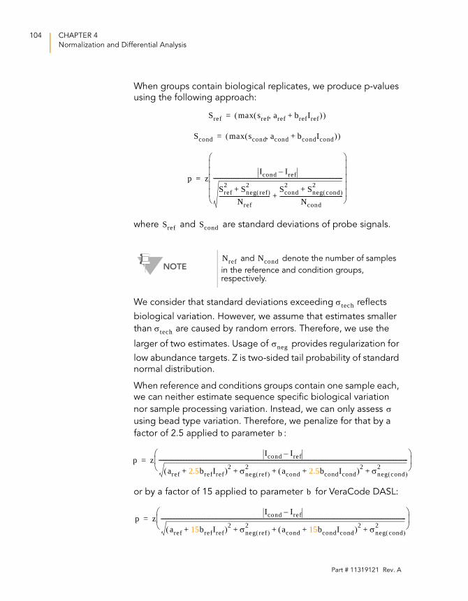
104 CHAPTER 4
Normalization and Differential Analysis
When groups contain biological replicates, we produce p-values
using the following approach:
where and are standard deviations of probe signals.
We consider that standard deviations exceeding reflects
biological variation. However, we assume that estimates smaller
than are caused by random errors. Therefore, we use the
larger of two estimates. Usage of provides regularization for
low abundance targets. Z is two-sided tail probability of standard
normal distribution.
When reference and conditions groups contain one sample each,
we can neither estimate sequence specific biological variation
nor sample processing variation. Instead, we can only assess
using bead type variation. Therefore, we penalize for that by a
factor of 2.5 applied to parameter :
or by a factor of 15 applied to parameter for VeraCode DASL:
NOTE and denote the number of samples
in the reference and condition groups, respectively.
Sref max sref aref brefIref+,( )( )=
Scond max scond acond bcondIcond+,( )( )=
p zIcond Iref–
Sref2 Sneg ref( )
2+Nref
------------------------------------Scond
2 Sneg cond( )2+
Ncond---------------------------------------------+
---------------------------------------------------------------------------------------------
⎝ ⎠⎜ ⎟⎜ ⎟⎜ ⎟⎜ ⎟⎜ ⎟⎛ ⎞
=
Sref Scond
Nref Ncond
σtech
σtech
σneg
σ
b
p zIcond Iref–
aref 2.5brefIref+( )2 σneg ref( )2 acond 2.5bcondIcond+( )2 σneg cond( )
2+ + +-----------------------------------------------------------------------------------------------------------------------------------------------------------------------------------⎝ ⎠⎜ ⎟⎛ ⎞
=
b
p zIcond Iref–
aref 15brefIref+( )2 σneg ref( )2 acond 15bcondIcond+( )2 σneg cond( )
2+ + +--------------------------------------------------------------------------------------------------------------------------------------------------------------------------------⎝ ⎠⎜ ⎟⎛ ⎞
=
Part # 11319121 Rev. A
Differential Expression Algorithms 105
These factors were determined empirically by examining real
sample data.
A Diff Score for a probe is computed as:
For the gene, Diff Scores of corresponding probes are averaged.
In addition, concordance between probes is reported.
Mann-Whitney This implementation produces exact p-value if:
or
Otherwise, normal approximation with continuity correction is
used. Differential scores are computed as described for the
Illumina Custom model (page 103).
T-Test When either the reference group or a condition group contains
at least two samples, variance is estimated across replicate
samples. Otherwise, variance is estimated from bead-to-bead
variation. We use t-test with the assumption of equal variance.
Differential scores are computed the same way as described for
the Illumina Custom model (page 103).
NOTE
For the DASL assay, the red and green channel signals are added together before computing diff scores.
DiffScore 10 Icond Iref–( )log10 p( )sgn( )=
min Nref Ncond,( ) 3<
max Nref Ncond,( ) 22<
GenomeStudio Gene Expression Module v1.0 User Guide

106 CHAPTER 4
Normalization and Differential Analysis
Detection P-Value
Detection p-value is a statistical calculation that provides the
probability that the signal from a given probe is greater than the
average signal from the negative controls.
WholeGenome
BeadChips
Detection p-value is calculated with the equation:
where R is the rank of the Z score of the analytical probes, and N
is the number of negative controls.
The Z score is calculated with the equation:
where and are the mean and the standard deviation of
signals of the negative controls on the ith sample and the
gth gene.
When samples are combined together to form a group, the Z
score is averaged:
The value for R is returned by a function that compares the Z
score for the probe intensity to the Z score of the
negative controls.
If the Z score for the probe intensity is smaller than the lowest
negative control Z score, the function returns a 0 and the
p-value is 1.
If the Z score for the probe intensity falls within the range of the Z
scores of the negative controls, R is the rank of the Z score of the
probe, and the p-value is in the range of 0 to 1.
If the Z score for the probe intensity is greater than the largest
negative control Z score, the function returns a 1 and the
p-value is 0.
DPV 1 RN----–=
ZigI μi
neg–
σineg
-------------------=
μineg σi
neg
Zig1m---- Zig
i∑=
Part # 11319121 Rev. A

Detection P-Value 107
DASL, miRNA,VeraCodeDASL, and
FocusedArrays
Because DASL, miRNA, VeraCode DASL, and Focused arrays
contain relatively few negative controls, GenomeStudio uses a
normal distribution to model their signals. For DASL products,
the Cy3 and Cy5 channels are added for the computation of
selected p-values.
The detection p-value is given by:
where F is 1 - the normal cumulative probability
distribution function.
For gene-level p-values, the calculation is as follows:
where N is the number of probes for gene g.
For groups containing multiple samples, the average Z score is
computed as described in Whole Genome BeadChips on
page 106. The detection p-value is then computed using the
following formula:
Where is the standard deviation of the average Z scores of
the negative controls.
p FIprobe μneg–
σneg-------------------------------⎝ ⎠⎛ ⎞=
p F NIgene μneg–
σneg--------------------------------⎝ ⎠
⎛ ⎞=
p FZgσzneg
-----------⎝ ⎠⎜ ⎟⎛ ⎞
=
σzneg
GenomeStudio Gene Expression Module v1.0 User Guide

108 CHAPTER 4
Normalization and Differential Analysis
Part # 11319121 Rev. A

Chapter 5
Analyzing miRNA Data
Topics110 Introduction
110 Importing an Analysis for Comparison
112 Loading a Lookup Table
113 Generating a Dendrogram
114 Identifying Correlated miRNA and mRNA Expression Values
117 Viewing miRNA Controls
GenomeStudio Gene Expression Module v1.0 User Guide
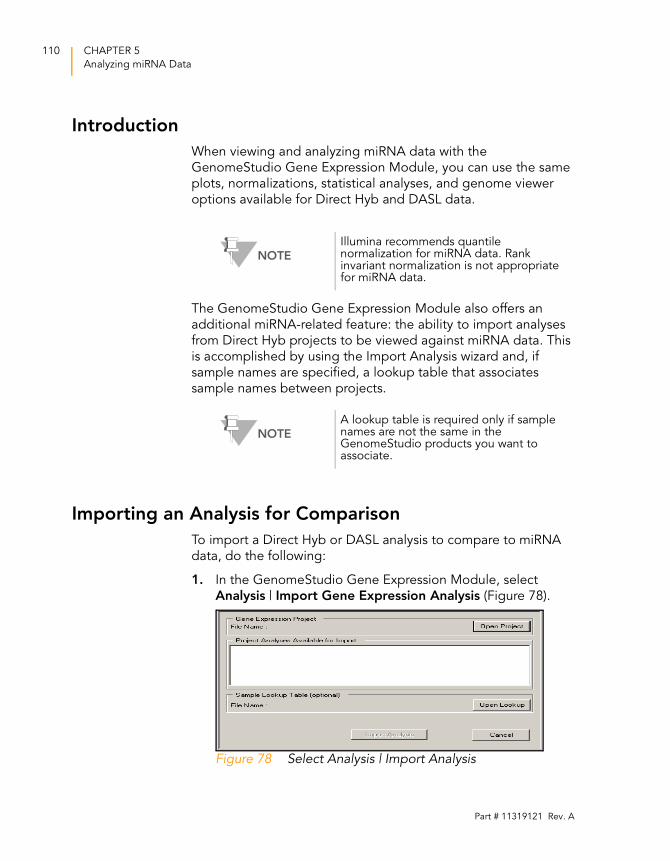
110 CHAPTER 5
Analyzing miRNA Data
Introduction
When viewing and analyzing miRNA data with the
GenomeStudio Gene Expression Module, you can use the same
plots, normalizations, statistical analyses, and genome viewer
options available for Direct Hyb and DASL data.
The GenomeStudio Gene Expression Module also offers an
additional miRNA-related feature: the ability to import analyses
from Direct Hyb projects to be viewed against miRNA data. This
is accomplished by using the Import Analysis wizard and, if
sample names are specified, a lookup table that associates
sample names between projects.
Importing an Analysis for Comparison
To import a Direct Hyb or DASL analysis to compare to miRNA
data, do the following:
1. In the GenomeStudio Gene Expression Module, select
Analysis | Import Gene Expression Analysis (Figure 78).
Figure 78 Select Analysis | Import Analysis
NOTE
Illumina recommends quantile normalization for miRNA data. Rank invariant normalization is not appropriate for miRNA data.
NOTE
A lookup table is required only if sample names are not the same in the GenomeStudio products you want to associate.
Part # 11319121 Rev. A
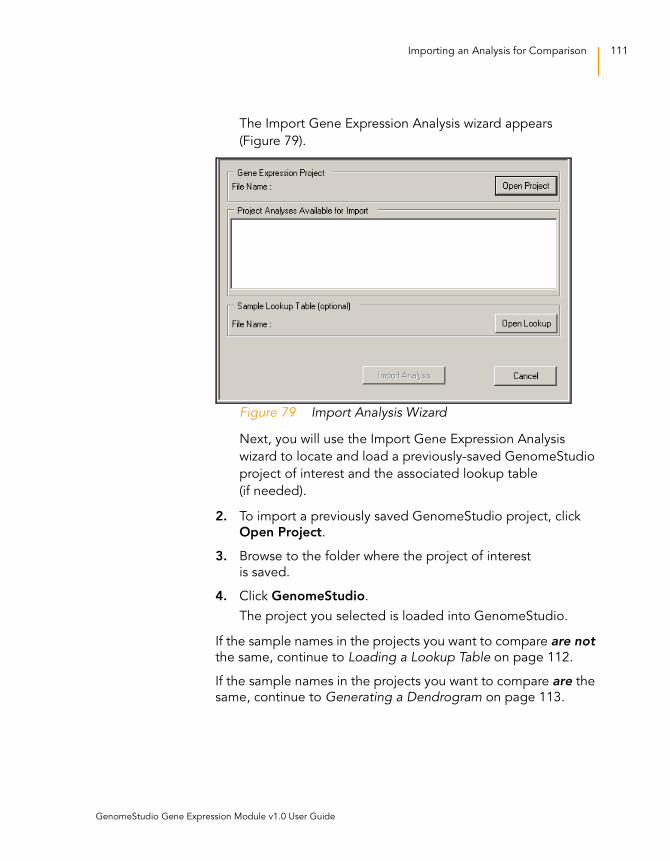
Importing an Analysis for Comparison 111
The Import Gene Expression Analysis wizard appears
(Figure 79).
Figure 79 Import Analysis Wizard
Next, you will use the Import Gene Expression Analysis
wizard to locate and load a previously-saved GenomeStudio
project of interest and the associated lookup table
(if needed).
2. To import a previously saved GenomeStudio project, click
Open Project.
3. Browse to the folder where the project of interest
is saved.
4. Click GenomeStudio.
The project you selected is loaded into GenomeStudio.
If the sample names in the projects you want to compare are not the same, continue to Loading a Lookup Table on page 112.
If the sample names in the projects you want to compare are the
same, continue to Generating a Dendrogram on page 113.
GenomeStudio Gene Expression Module v1.0 User Guide
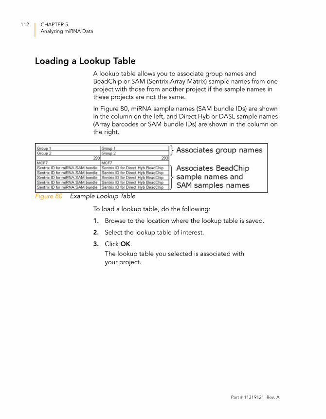
112 CHAPTER 5
Analyzing miRNA Data
Loading a Lookup Table
A lookup table allows you to associate group names and
BeadChip or SAM (Sentrix Array Matrix) sample names from one
project with those from another project if the sample names in
these projects are not the same.
In Figure 80, miRNA sample names (SAM bundle IDs) are shown
in the column on the left, and Direct Hyb or DASL sample names
(Array barcodes or SAM bundle IDs) are shown in the column on
the right.
Figure 80 Example Lookup Table
To load a lookup table, do the following:
1. Browse to the location where the lookup table is saved.
2. Select the lookup table of interest.
3. Click OK.
The lookup table you selected is associated with
your project.
Part # 11319121 Rev. A
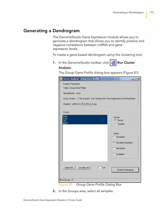
Generating a Dendrogram 113
Generating a Dendrogram
The GenomeStudio Gene Expression module allows you to
generate a dendrogram that allows you to identify positive and
negative correlations between miRNA and gene
expression levels.
To create a gene-based dendrogram using the clustering tool:
1. In the GenomeStudio toolbar, click Run Cluster
Analysis.
The Group Gene Profile dialog box appears (Figure 81).
Figure 81 Group Gene Profile Dialog Box
2. In the Groups area, select all samples.
GenomeStudio Gene Expression Module v1.0 User Guide
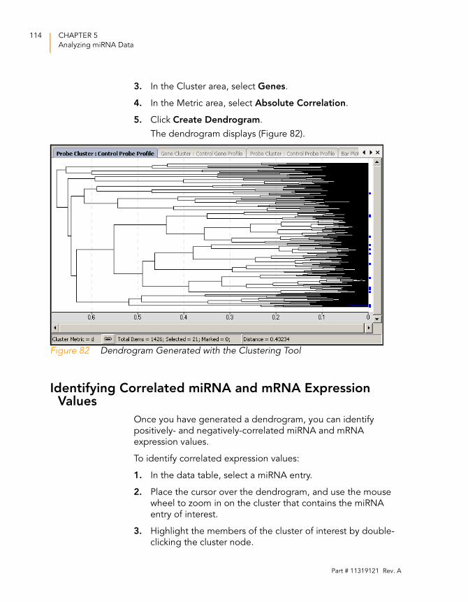
114 CHAPTER 5
Analyzing miRNA Data
3. In the Cluster area, select Genes.
4. In the Metric area, select Absolute Correlation.
5. Click Create Dendrogram.
The dendrogram displays (Figure 82).
Figure 82 Dendrogram Generated with the Clustering Tool
Identifying Correlated miRNA and mRNA Expression Values
Once you have generated a dendrogram, you can identify
positively- and negatively-correlated miRNA and mRNA
expression values.
To identify correlated expression values:
1. In the data table, select a miRNA entry.
2. Place the cursor over the dendrogram, and use the mouse
wheel to zoom in on the cluster that contains the miRNA
entry of interest.
3. Highlight the members of the cluster of interest by double-
clicking the cluster node.
Part # 11319121 Rev. A
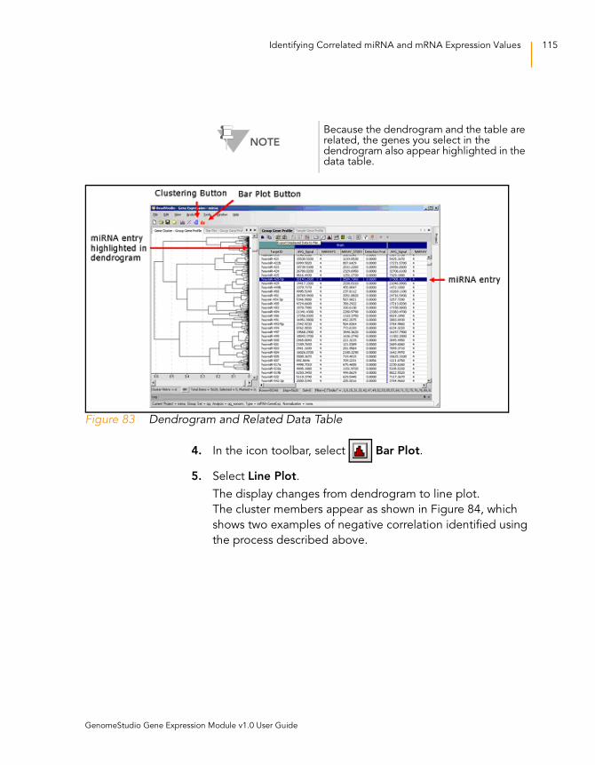
Identifying Correlated miRNA and mRNA Expression Values 115
Figure 83 Dendrogram and Related Data Table
4. In the icon toolbar, select Bar Plot.
5. Select Line Plot.
The display changes from dendrogram to line plot.
The cluster members appear as shown in Figure 84, which
shows two examples of negative correlation identified using
the process described above.
NOTE
Because the dendrogram and the table are related, the genes you select in the dendrogram also appear highlighted in the data table.
GenomeStudio Gene Expression Module v1.0 User Guide
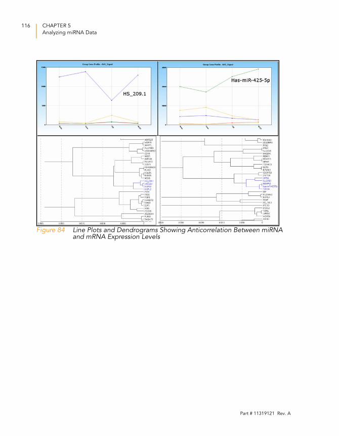
116 CHAPTER 5
Analyzing miRNA Data
Figure 84 Line Plots and Dendrograms Showing Anticorrelation Between miRNA and mRNA Expression Levels
Part # 11319121 Rev. A
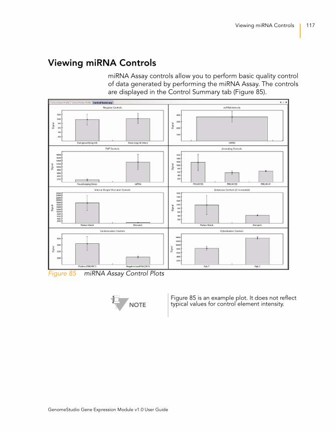
Viewing miRNA Controls 117
Viewing miRNA Controls
miRNA Assay controls allow you to perform basic quality control
of data generated by performing the miRNA Assay. The controls
are displayed in the Control Summary tab (Figure 85).
Figure 85 miRNA Assay Control Plots
NOTE
Figure 85 is an example plot. It does not reflect typical values for control element intensity.
GenomeStudio Gene Expression Module v1.0 User Guide
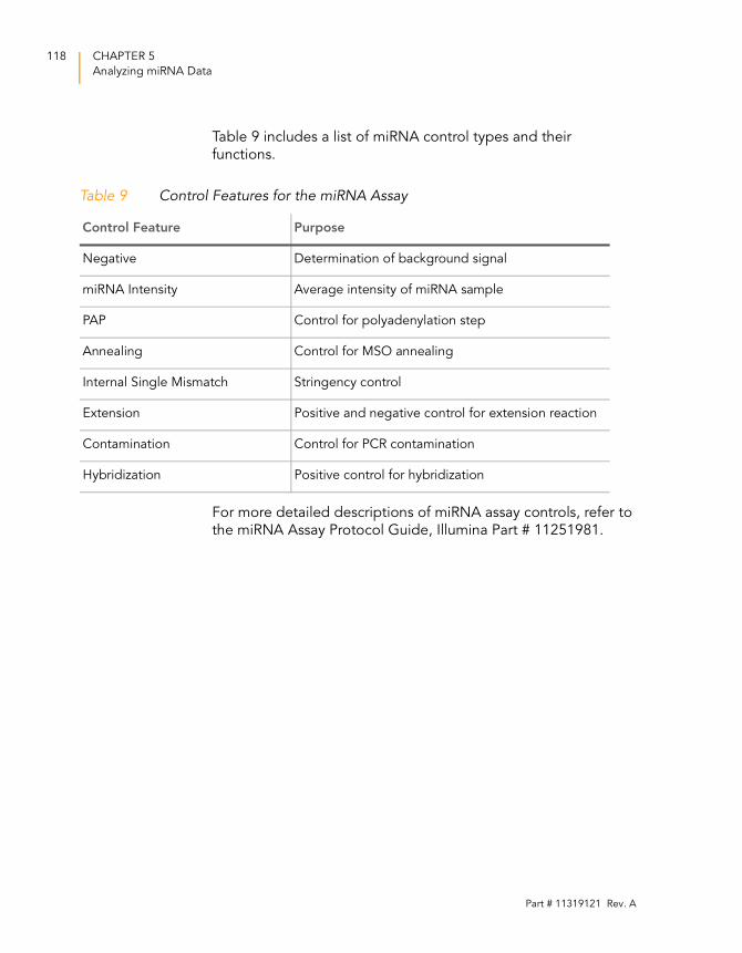
118 CHAPTER 5
Analyzing miRNA Data
Table 9 includes a list of miRNA control types and their
functions.
For more detailed descriptions of miRNA assay controls, refer to
the miRNA Assay Protocol Guide, Illumina Part # 11251981.
Table 9 Control Features for the miRNA Assay
Control Feature Purpose
Negative Determination of background signal
miRNA Intensity Average intensity of miRNA sample
PAP Control for polyadenylation step
Annealing Control for MSO annealing
Internal Single Mismatch Stringency control
Extension Positive and negative control for extension reaction
Contamination Control for PCR contamination
Hybridization Positive control for hybridization
Part # 11319121 Rev. A

Chapter 6
Generating a Final
Report
Topics120 Introduction
120 Generating a Final Report
124 Viewing a Final Report
GenomeStudio Gene Expression Module v1.0 User Guide
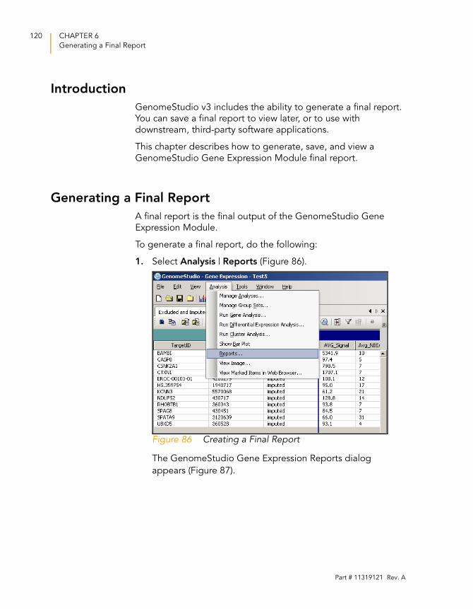
120 CHAPTER 6
Generating a Final Report
Introduction
GenomeStudio v3 includes the ability to generate a final report.
You can save a final report to view later, or to use with
downstream, third-party software applications.
This chapter describes how to generate, save, and view a
GenomeStudio Gene Expression Module final report.
Generating a Final Report
A final report is the final output of the GenomeStudio Gene
Expression Module.
To generate a final report, do the following:
1. Select Analysis | Reports (Figure 86).
Figure 86 Creating a Final Report
The GenomeStudio Gene Expression Reports dialog
appears (Figure 87).
Part # 11319121 Rev. A
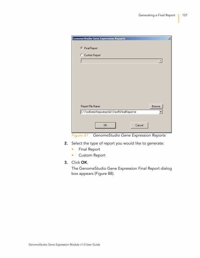
Generating a Final Report 121
Figure 87 GenomeStudio Gene Expression Reports
2. Select the type of report you would like to generate:
• Final Report
• Custom Report
3. Click OK.
The GenomeStudio Gene Expression Final Report dialog
box appears (Figure 88).
GenomeStudio Gene Expression Module v1.0 User Guide
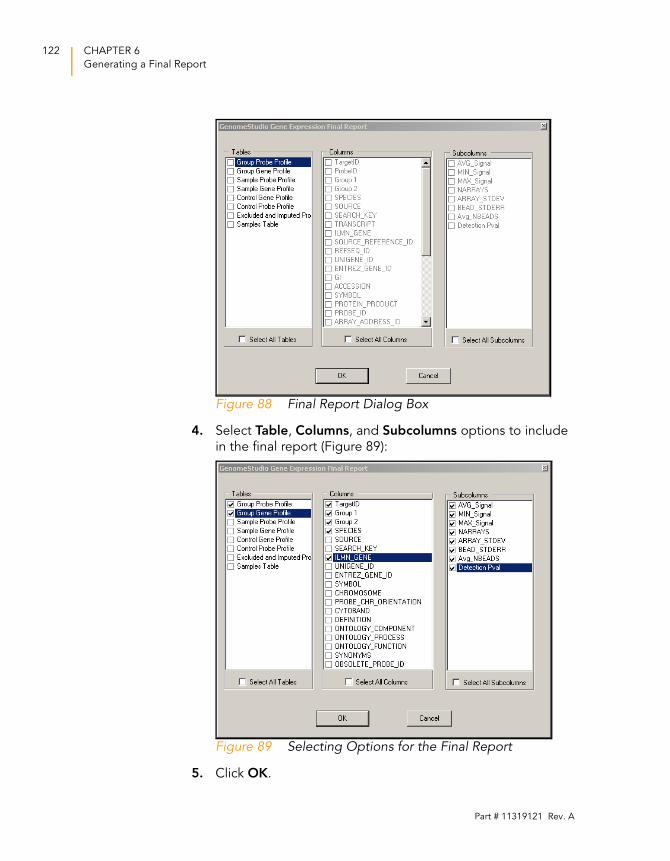
122 CHAPTER 6
Generating a Final Report
Figure 88 Final Report Dialog Box
4. Select Table, Columns, and Subcolumns options to include
in the final report (Figure 89):
Figure 89 Selecting Options for the Final Report
5. Click OK.
Part # 11319121 Rev. A
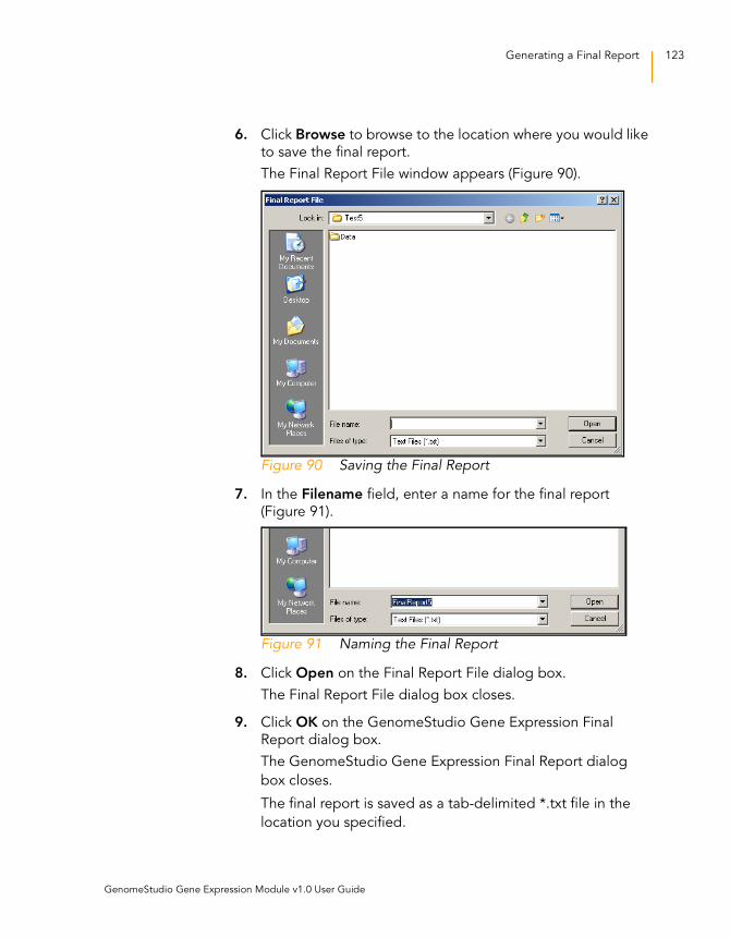
Generating a Final Report 123
6. Click Browse to browse to the location where you would like
to save the final report.
The Final Report File window appears (Figure 90).
Figure 90 Saving the Final Report
7. In the Filename field, enter a name for the final report
(Figure 91).
Figure 91 Naming the Final Report
8. Click Open on the Final Report File dialog box.
The Final Report File dialog box closes.
9. Click OK on the GenomeStudio Gene Expression Final
Report dialog box.
The GenomeStudio Gene Expression Final Report dialog
box closes.
The final report is saved as a tab-delimited *.txt file in the
location you specified.
GenomeStudio Gene Expression Module v1.0 User Guide
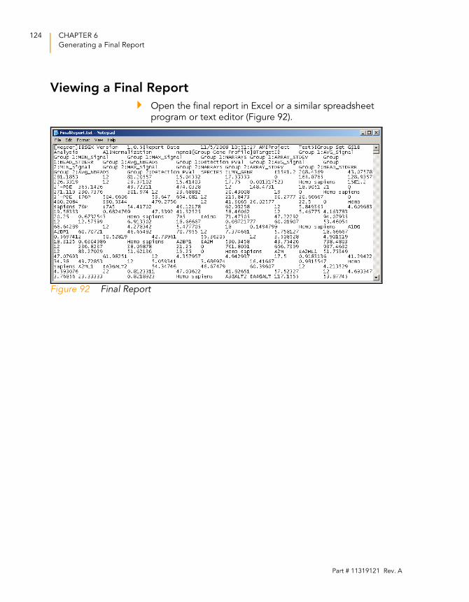
124 CHAPTER 6
Generating a Final Report
Viewing a Final Report
Open the final report in Excel or a similar spreadsheet
program or text editor (Figure 92).
Figure 92 Final Report
Part # 11319121 Rev. A
Chapter 7
User Interface Reference
Topics126 Introduction
126 Detachable Docking Windows
127 Line Plot, Group Gene Profile
128 Samples Table
130 Group Gene Profile
135 Group Probe Profile
139 Sample Gene Profile
143 Sample Probe Profile
146 Control Gene Profile
149 Control Probe Profile
151 Excluded and Imputed Probes Table
153 Control Summary
157 Project Window
157 Log Window
159 Main Window Menus
163 Context Menus
GenomeStudio Gene Expression Module v1.0 User Guide
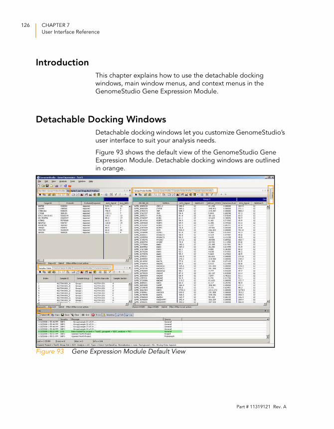
126 CHAPTER 7
User Interface Reference
Introduction
This chapter explains how to use the detachable docking
windows, main window menus, and context menus in the
GenomeStudio Gene Expression Module.
Detachable Docking Windows
Detachable docking windows let you customize GenomeStudio’s
user interface to suit your analysis needs.
Figure 93 shows the default view of the GenomeStudio Gene
Expression Module. Detachable docking windows are outlined
in orange.
Figure 93 Gene Expression Module Default View
Part # 11319121 Rev. A
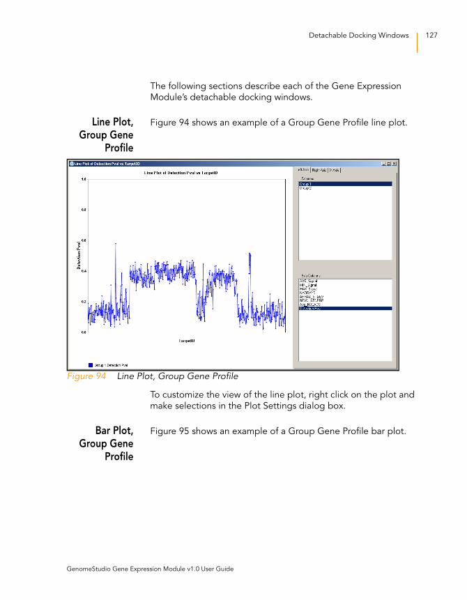
Detachable Docking Windows 127
The following sections describe each of the Gene Expression
Module’s detachable docking windows.
Line Plot,Group Gene
Profile
Figure 94 shows an example of a Group Gene Profile line plot.
Figure 94 Line Plot, Group Gene Profile
To customize the view of the line plot, right click on the plot and
make selections in the Plot Settings dialog box.
Bar Plot,Group Gene
Profile
Figure 95 shows an example of a Group Gene Profile bar plot.
GenomeStudio Gene Expression Module v1.0 User Guide
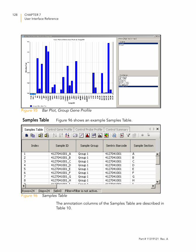
128 CHAPTER 7
User Interface Reference
Figure 95 Bar Plot, Group Gene Profile
Samples Table Figure 96 shows an example Samples Table.
Figure 96 Samples Table
The annotation columns of the Samples Table are described in
Table 10.
Part # 11319121 Rev. A
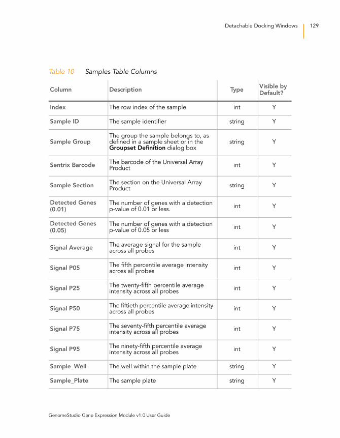
Detachable Docking Windows 129
Table 10 Samples Table Columns
Column Description TypeVisible by Default?
Index The row index of the sample int Y
Sample ID The sample identifier string Y
Sample GroupThe group the sample belongs to, as defined in a sample sheet or in the Groupset Definition dialog box
string Y
Sentrix BarcodeThe barcode of the Universal Array Product
int Y
Sample SectionThe section on the Universal Array Product
string Y
Detected Genes (0.01)
The number of genes with a detection p-value of 0.01 or less.
int Y
Detected Genes (0.05)
The number of genes with a detection p-value of 0.05 or less
int Y
Signal AverageThe average signal for the sample across all probes
int Y
Signal P05The fifth percentile average intensity across all probes
int Y
Signal P25The twenty-fifth percentile average intensity across all probes
int Y
Signal P50The fiftieth percentile average intensity across all probes
int Y
Signal P75The seventy-fifth percentile average intensity across all probes
int Y
Signal P95The ninety-fifth percentile average intensity across all probes
int Y
Sample_Well The well within the sample plate string Y
Sample_Plate The sample plate string Y
GenomeStudio Gene Expression Module v1.0 User Guide
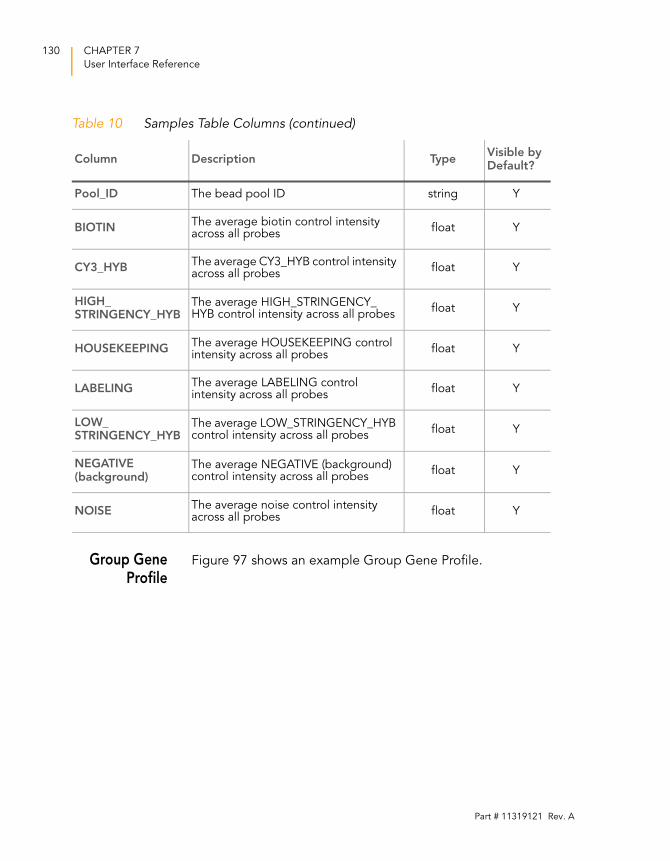
130 CHAPTER 7
User Interface Reference
Group GeneProfile
Figure 97 shows an example Group Gene Profile.
Pool_ID The bead pool ID string Y
BIOTINThe average biotin control intensity across all probes
float Y
CY3_HYBThe average CY3_HYB control intensity across all probes
float Y
HIGH_STRINGENCY_HYB
The average HIGH_STRINGENCY_HYB control intensity across all probes
float Y
HOUSEKEEPINGThe average HOUSEKEEPING control intensity across all probes
float Y
LABELINGThe average LABELING control intensity across all probes
float Y
LOW_STRINGENCY_HYB
The average LOW_STRINGENCY_HYB control intensity across all probes
float Y
NEGATIVE (background)
The average NEGATIVE (background) control intensity across all probes
float Y
NOISEThe average noise control intensity across all probes
float Y
Table 10 Samples Table Columns (continued)
Column Description TypeVisible by Default?
Part # 11319121 Rev. A
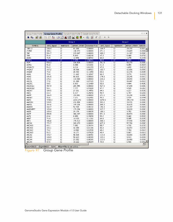
Detachable Docking Windows 131
Figure 97 Group Gene Profile
GenomeStudio Gene Expression Module v1.0 User Guide
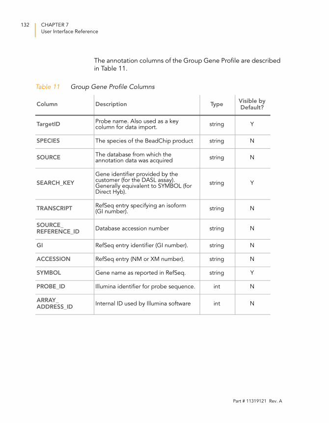
132 CHAPTER 7
User Interface Reference
The annotation columns of the Group Gene Profile are described
in Table 11.
Table 11 Group Gene Profile Columns
Column Description TypeVisible by Default?
TargetIDProbe name. Also used as a key column for data import.
string Y
SPECIES The species of the BeadChip product string N
SOURCEThe database from which the annotation data was acquired
string N
SEARCH_KEY
Gene identifier provided by the customer (for the DASL assay). Generally equivalent to SYMBOL (for Direct Hyb).
string Y
TRANSCRIPTRefSeq entry specifying an isoform (GI number).
string N
SOURCE_REFERENCE_ID
Database accession number string N
GI RefSeq entry identifier (GI number). string N
ACCESSION RefSeq entry (NM or XM number). string N
SYMBOL Gene name as reported in RefSeq. string Y
PROBE_ID Illumina identifier for probe sequence. int N
ARRAY_ADDRESS_ID
Internal ID used by Illumina software int N
Part # 11319121 Rev. A
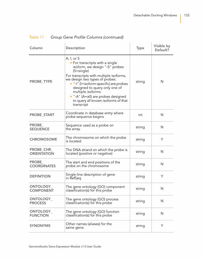
Detachable Docking Windows 133
PROBE_TYPE
A, I, or S
• For transcripts with a single isoform, we design "-S" probes (S=single)
For transcripts with multiple isoforms, we design two types of probes:
• "-I" (I=isoform-specific) are probes designed to query only one of multiple isoforms
• "-A" (A=all) are probes designed to query all known isoforms of that transcript
string N
PROBE_STARTCoordinate in database entry where probe sequence begins
int N
PROBE_SEQUENCE
Sequence used as a probe on the array.
string N
CHROMOSOMEThe chromosome on which the probe is located
string Y
PROBE_CHR_ORIENTATION
The DNA strand on which the probe is located (positive or negative)
string N
PROBE_COORDINATES
The start and end positions of the probe on the chromosome
string N
DEFINITIONSingle-line description of gene in RefSeq
string Y
ONTOLOGY_COMPONENT
The gene ontology (GO) component classification(s) for this probe
string N
ONTOLOGY_PROCESS
The gene ontology (GO) process classification(s) for this probe
string N
ONTOLOGY_FUNCTION
The gene ontology (GO) function classification(s) for this probe
string N
SYNONYMSOther names (aliases) for the same gene.
string Y
Table 11 Group Gene Profile Columns (continued)
Column Description TypeVisible by Default?
GenomeStudio Gene Expression Module v1.0 User Guide
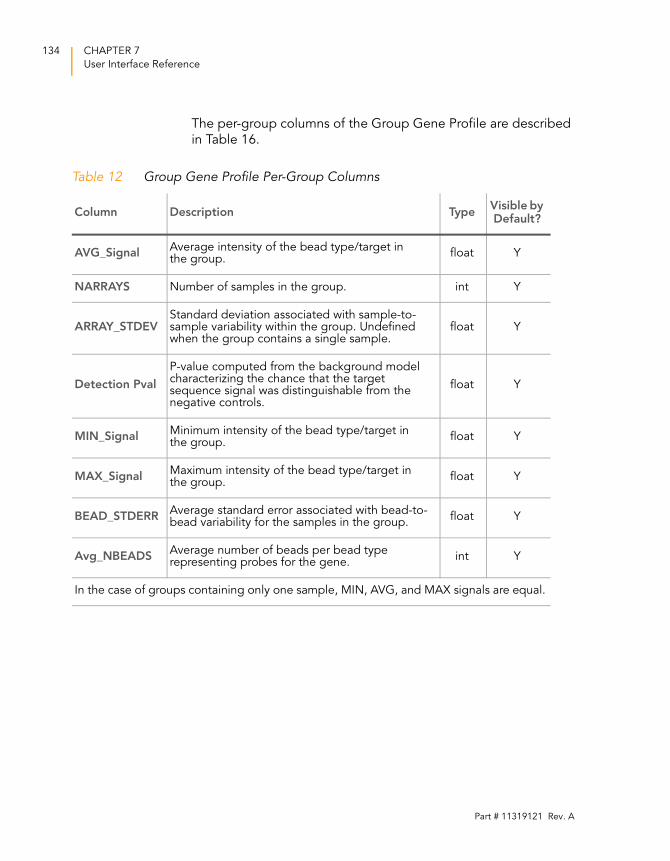
134 CHAPTER 7
User Interface Reference
The per-group columns of the Group Gene Profile are described
in Table 16.
Table 12 Group Gene Profile Per-Group Columns
Column Description TypeVisible by Default?
AVG_SignalAverage intensity of the bead type/target in the group.
float Y
NARRAYS Number of samples in the group. int Y
ARRAY_STDEVStandard deviation associated with sample-to-sample variability within the group. Undefined when the group contains a single sample.
float Y
Detection Pval
P-value computed from the background model characterizing the chance that the target sequence signal was distinguishable from the negative controls.
float Y
MIN_SignalMinimum intensity of the bead type/target in the group.
float Y
MAX_SignalMaximum intensity of the bead type/target in the group.
float Y
BEAD_STDERRAverage standard error associated with bead-to-bead variability for the samples in the group.
float Y
Avg_NBEADSAverage number of beads per bead type representing probes for the gene.
int Y
In the case of groups containing only one sample, MIN, AVG, and MAX signals are equal.
Part # 11319121 Rev. A
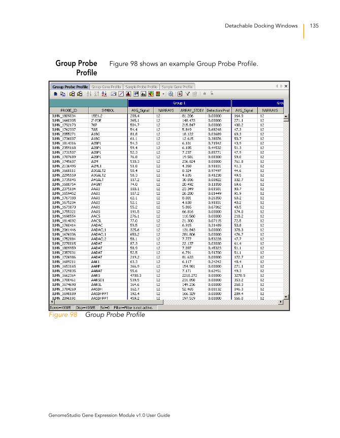
Detachable Docking Windows 135
Group ProbeProfile
Figure 98 shows an example Group Probe Profile.
Figure 98 Group Probe Profile
GenomeStudio Gene Expression Module v1.0 User Guide
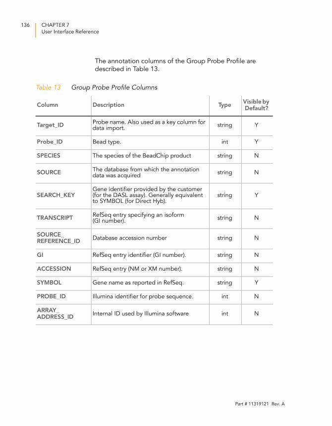
136 CHAPTER 7
User Interface Reference
The annotation columns of the Group Probe Profile are
described in Table 13.
Table 13 Group Probe Profile Columns
Column Description TypeVisible by Default?
Target_IDProbe name. Also used as a key column for data import.
string Y
Probe_ID Bead type. int Y
SPECIES The species of the BeadChip product string N
SOURCEThe database from which the annotation data was acquired
string N
SEARCH_KEYGene identifier provided by the customer (for the DASL assay). Generally equivalent to SYMBOL (for Direct Hyb).
string Y
TRANSCRIPTRefSeq entry specifying an isoform (GI number).
string N
SOURCE_REFERENCE_ID
Database accession number string N
GI RefSeq entry identifier (GI number). string N
ACCESSION RefSeq entry (NM or XM number). string N
SYMBOL Gene name as reported in RefSeq. string Y
PROBE_ID Illumina identifier for probe sequence. int N
ARRAY_ADDRESS_ID
Internal ID used by Illumina software int N
Part # 11319121 Rev. A
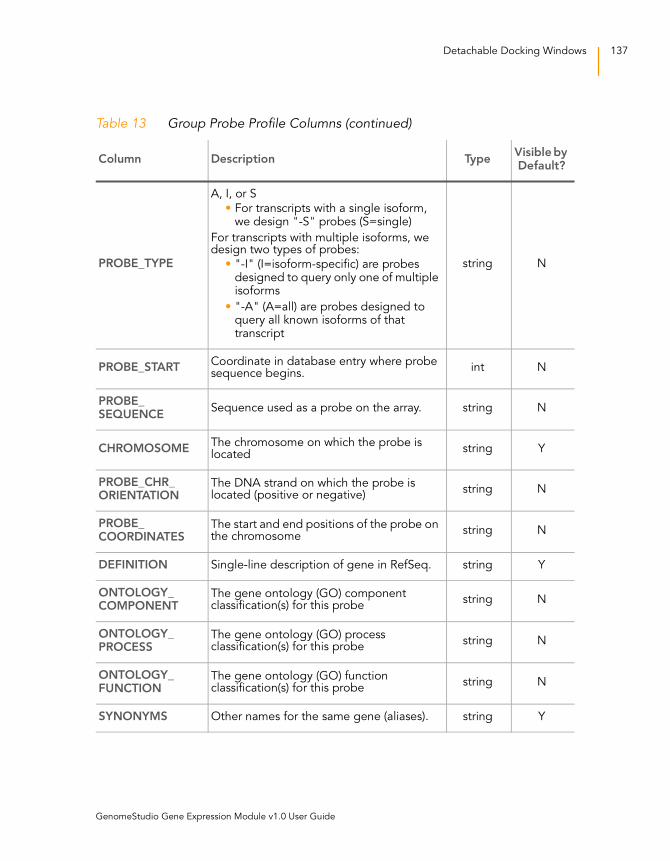
Detachable Docking Windows 137
PROBE_TYPE
A, I, or S
• For transcripts with a single isoform, we design "-S" probes (S=single)
For transcripts with multiple isoforms, we design two types of probes:
• "-I" (I=isoform-specific) are probes designed to query only one of multiple isoforms
• "-A" (A=all) are probes designed to query all known isoforms of that transcript
string N
PROBE_STARTCoordinate in database entry where probe sequence begins.
int N
PROBE_SEQUENCE
Sequence used as a probe on the array. string N
CHROMOSOMEThe chromosome on which the probe is located
string Y
PROBE_CHR_ORIENTATION
The DNA strand on which the probe is located (positive or negative)
string N
PROBE_COORDINATES
The start and end positions of the probe on the chromosome
string N
DEFINITION Single-line description of gene in RefSeq. string Y
ONTOLOGY_COMPONENT
The gene ontology (GO) component classification(s) for this probe
string N
ONTOLOGY_PROCESS
The gene ontology (GO) process classification(s) for this probe
string N
ONTOLOGY_FUNCTION
The gene ontology (GO) function classification(s) for this probe
string N
SYNONYMS Other names for the same gene (aliases). string Y
Table 13 Group Probe Profile Columns (continued)
Column Description TypeVisible by Default?
GenomeStudio Gene Expression Module v1.0 User Guide
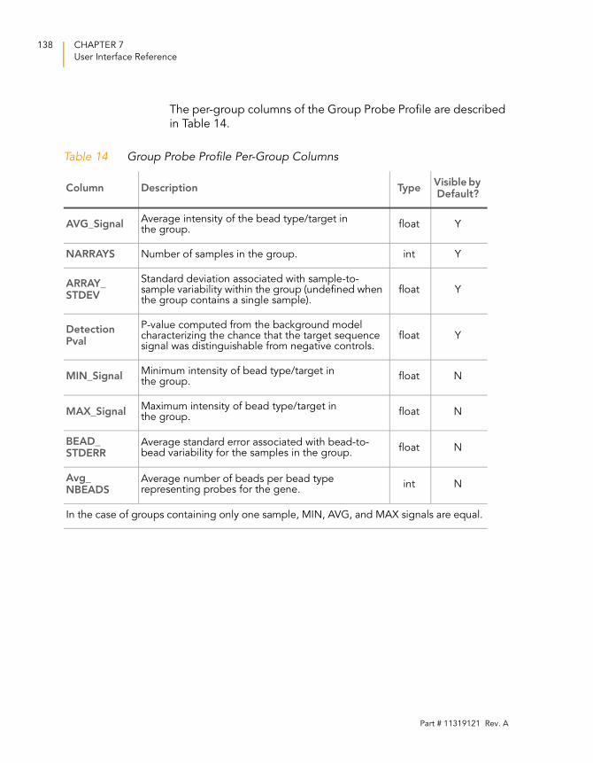
138 CHAPTER 7
User Interface Reference
The per-group columns of the Group Probe Profile are described
in Table 14.
Table 14 Group Probe Profile Per-Group Columns
Column Description TypeVisible by Default?
AVG_SignalAverage intensity of the bead type/target in the group.
float Y
NARRAYS Number of samples in the group. int Y
ARRAY_STDEV
Standard deviation associated with sample-to-sample variability within the group (undefined when the group contains a single sample).
float Y
Detection Pval
P-value computed from the background model characterizing the chance that the target sequence signal was distinguishable from negative controls.
float Y
MIN_SignalMinimum intensity of bead type/target in the group.
float N
MAX_SignalMaximum intensity of bead type/target in the group.
float N
BEAD_STDERR
Average standard error associated with bead-to-bead variability for the samples in the group.
float N
Avg_NBEADS
Average number of beads per bead type representing probes for the gene.
int N
In the case of groups containing only one sample, MIN, AVG, and MAX signals are equal.
Part # 11319121 Rev. A
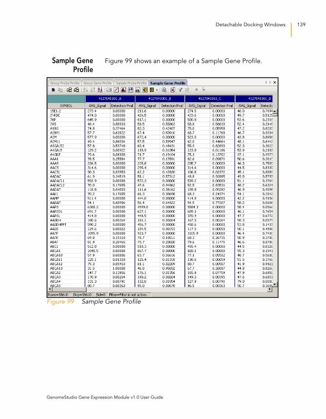
Detachable Docking Windows 139
Sample GeneProfile
Figure 99 shows an example of a Sample Gene Profile.
Figure 99 Sample Gene Profile
GenomeStudio Gene Expression Module v1.0 User Guide
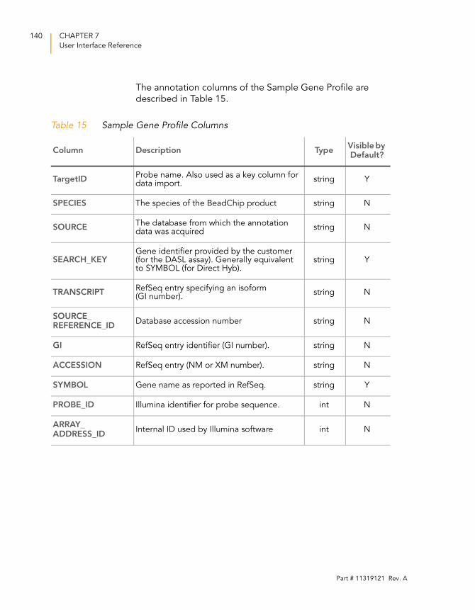
140 CHAPTER 7
User Interface Reference
The annotation columns of the Sample Gene Profile are
described in Table 15.
Table 15 Sample Gene Profile Columns
Column Description TypeVisible by Default?
TargetIDProbe name. Also used as a key column for data import.
string Y
SPECIES The species of the BeadChip product string N
SOURCEThe database from which the annotation data was acquired
string N
SEARCH_KEYGene identifier provided by the customer (for the DASL assay). Generally equivalent to SYMBOL (for Direct Hyb).
string Y
TRANSCRIPTRefSeq entry specifying an isoform (GI number).
string N
SOURCE_REFERENCE_ID
Database accession number string N
GI RefSeq entry identifier (GI number). string N
ACCESSION RefSeq entry (NM or XM number). string N
SYMBOL Gene name as reported in RefSeq. string Y
PROBE_ID Illumina identifier for probe sequence. int N
ARRAY_ADDRESS_ID
Internal ID used by Illumina software int N
Part # 11319121 Rev. A
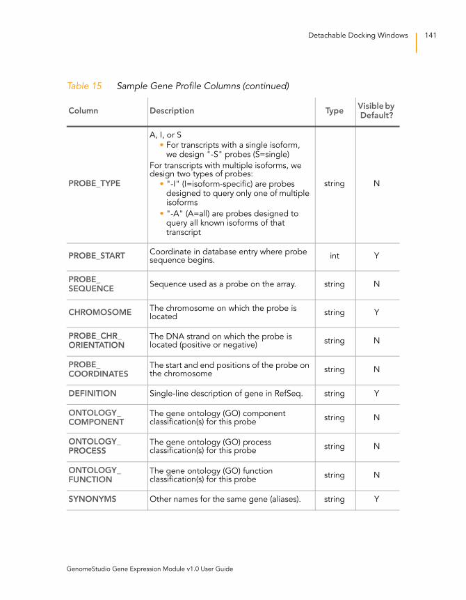
Detachable Docking Windows 141
PROBE_TYPE
A, I, or S
• For transcripts with a single isoform, we design "-S" probes (S=single)
For transcripts with multiple isoforms, we design two types of probes:
• "-I" (I=isoform-specific) are probes designed to query only one of multiple isoforms
• "-A" (A=all) are probes designed to query all known isoforms of that transcript
string N
PROBE_STARTCoordinate in database entry where probe sequence begins.
int Y
PROBE_SEQUENCE
Sequence used as a probe on the array. string N
CHROMOSOMEThe chromosome on which the probe is located
string Y
PROBE_CHR_ORIENTATION
The DNA strand on which the probe is located (positive or negative)
string N
PROBE_COORDINATES
The start and end positions of the probe on the chromosome
string N
DEFINITION Single-line description of gene in RefSeq. string Y
ONTOLOGY_COMPONENT
The gene ontology (GO) component classification(s) for this probe
string N
ONTOLOGY_PROCESS
The gene ontology (GO) process classification(s) for this probe
string N
ONTOLOGY_FUNCTION
The gene ontology (GO) function classification(s) for this probe
string N
SYNONYMS Other names for the same gene (aliases). string Y
Table 15 Sample Gene Profile Columns (continued)
Column Description TypeVisible by Default?
GenomeStudio Gene Expression Module v1.0 User Guide
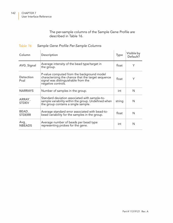
142 CHAPTER 7
User Interface Reference
The per-sample columns of the Sample Gene Profile are
described in Table 16.
Table 16 Sample Gene Profile Per-Sample Columns
Column Description TypeVisible by Default?
AVG_SignalAverage intensity of the bead type/target in the group.
float Y
Detection Pval
P-value computed from the background model characterizing the chance that the target sequence signal was distinguishable from the negative controls.
float Y
NARRAYS Number of samples in the group. int N
ARRAY_STDEV
Standard deviation associated with sample-to-sample variability within the group. Undefined when the group contains a single sample.
string N
BEAD_STDERR
Average standard error associated with bead-to-bead variability for the samples in the group.
float N
Avg_NBEADS
Average number of beads per bead type representing probes for the gene.
int N
Part # 11319121 Rev. A
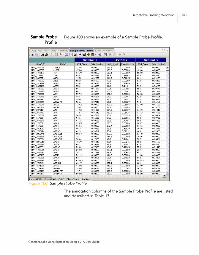
Detachable Docking Windows 143
Sample ProbeProfile
Figure 100 shows an example of a Sample Probe Profile.
Figure 100 Sample Probe Profile
The annotation columns of the Sample Probe Profile are listed
and described in Table 17.
GenomeStudio Gene Expression Module v1.0 User Guide
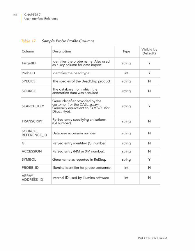
144 CHAPTER 7
User Interface Reference
Table 17 Sample Probe Profile Columns
Column Description TypeVisible by Default?
TargetIDIdentifies the probe name. Also used as a key column for data import.
string Y
ProbeID Identifies the bead type. int Y
SPECIES The species of the BeadChip product string N
SOURCEThe database from which the annotation data was acquired
string N
SEARCH_KEY
Gene identifier provided by the customer (for the DASL assay). Generally equivalent to SYMBOL (for Direct Hyb).
string Y
TRANSCRIPTRefSeq entry specifying an isoform (GI number).
string N
SOURCE_REFERENCE_ID
Database accession number string N
GI RefSeq entry identifier (GI number). string N
ACCESSION RefSeq entry (NM or XM number). string N
SYMBOL Gene name as reported in RefSeq. string Y
PROBE_ID Illumina identifier for probe sequence. int N
ARRAY_ADDRESS_ID
Internal ID used by Illumina software int N
Part # 11319121 Rev. A
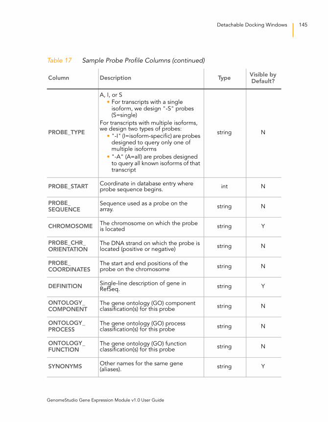
Detachable Docking Windows 145
PROBE_TYPE
A, I, or S
• For transcripts with a single isoform, we design "-S" probes (S=single)
For transcripts with multiple isoforms, we design two types of probes:
• "-I" (I=isoform-specific) are probes designed to query only one of multiple isoforms
• "-A" (A=all) are probes designed to query all known isoforms of that transcript
string N
PROBE_STARTCoordinate in database entry where probe sequence begins.
int N
PROBE_SEQUENCE
Sequence used as a probe on the array.
string N
CHROMOSOMEThe chromosome on which the probe is located
string Y
PROBE_CHR_ORIENTATION
The DNA strand on which the probe is located (positive or negative)
string N
PROBE_COORDINATES
The start and end positions of the probe on the chromosome
string N
DEFINITIONSingle-line description of gene in RefSeq.
string Y
ONTOLOGY_COMPONENT
The gene ontology (GO) component classification(s) for this probe
string N
ONTOLOGY_PROCESS
The gene ontology (GO) process classification(s) for this probe
string N
ONTOLOGY_FUNCTION
The gene ontology (GO) function classification(s) for this probe
string N
SYNONYMSOther names for the same gene (aliases).
string Y
Table 17 Sample Probe Profile Columns (continued)
Column Description TypeVisible by Default?
GenomeStudio Gene Expression Module v1.0 User Guide
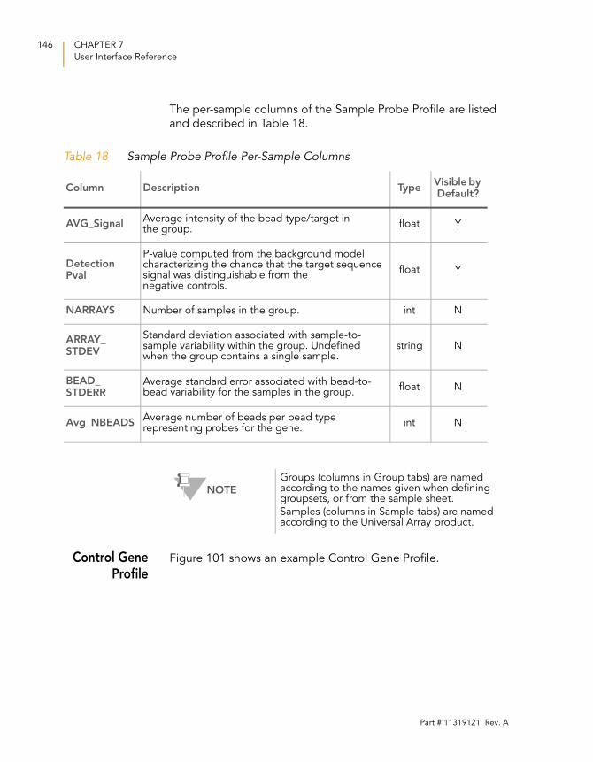
146 CHAPTER 7
User Interface Reference
The per-sample columns of the Sample Probe Profile are listed
and described in Table 18.
Control GeneProfile
Figure 101 shows an example Control Gene Profile.
Table 18 Sample Probe Profile Per-Sample Columns
Column Description TypeVisible by Default?
AVG_SignalAverage intensity of the bead type/target in the group.
float Y
Detection Pval
P-value computed from the background model characterizing the chance that the target sequence signal was distinguishable from the negative controls.
float Y
NARRAYS Number of samples in the group. int N
ARRAY_STDEV
Standard deviation associated with sample-to-sample variability within the group. Undefined when the group contains a single sample.
string N
BEAD_STDERR
Average standard error associated with bead-to-bead variability for the samples in the group.
float N
Avg_NBEADSAverage number of beads per bead type representing probes for the gene.
int N
NOTE
Groups (columns in Group tabs) are named according to the names given when defining groupsets, or from the sample sheet.
Samples (columns in Sample tabs) are named according to the Universal Array product.
Part # 11319121 Rev. A
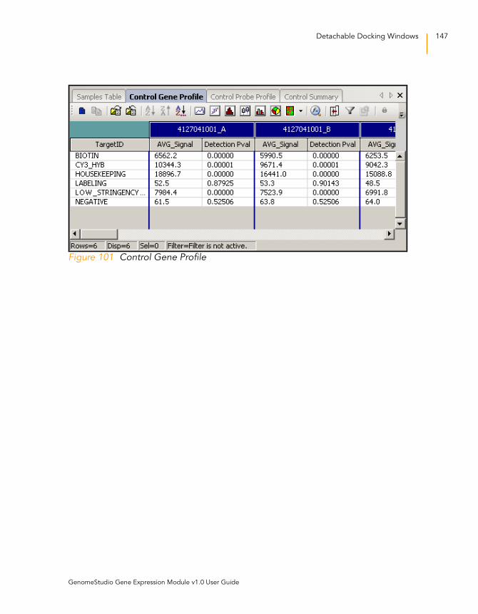
Detachable Docking Windows 147
Figure 101 Control Gene Profile
GenomeStudio Gene Expression Module v1.0 User Guide
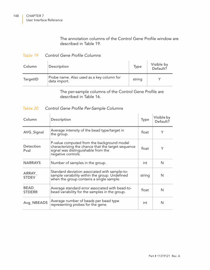
148 CHAPTER 7
User Interface Reference
The annotation columns of the Control Gene Profile window are
described in Table 19.
The per-sample columns of the Control Gene Profile are
described in Table 16.
Table 19 Control Gene Profile Columns
Column Description TypeVisible by Default?
TargetIDProbe name. Also used as a key column for data import.
string Y
Table 20 Control Gene Profile Per-Sample Columns
Column Description TypeVisible by Default?
AVG_SignalAverage intensity of the bead type/target in the group.
float Y
Detection Pval
P-value computed from the background model characterizing the chance that the target sequence signal was distinguishable from the negative controls.
float Y
NARRAYS Number of samples in the group. int N
ARRAY_STDEV
Standard deviation associated with sample-to-sample variability within the group. Undefined when the group contains a single sample.
string N
BEAD_STDERR
Average standard error associated with bead-to-bead variability for the samples in the group.
float N
Avg_NBEADSAverage number of beads per bead type representing probes for the gene.
int N
Part # 11319121 Rev. A
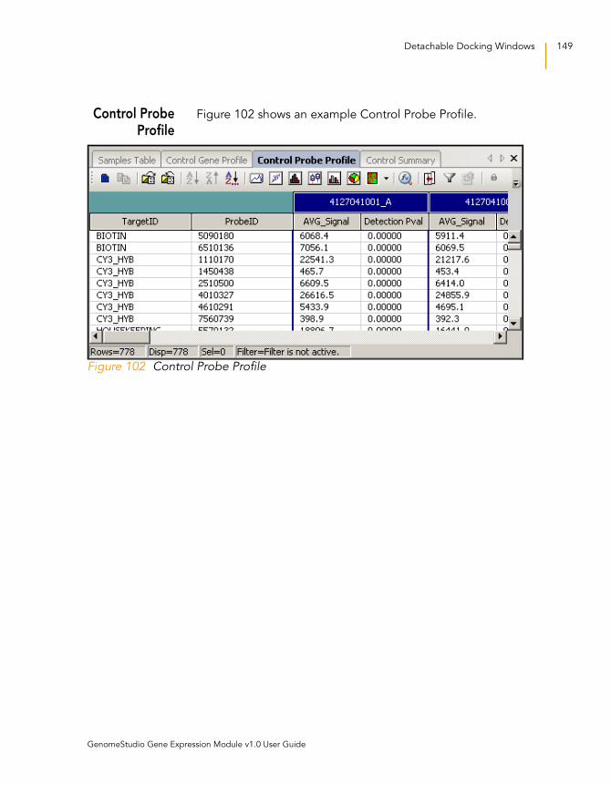
Detachable Docking Windows 149
Control ProbeProfile
Figure 102 shows an example Control Probe Profile.
Figure 102 Control Probe Profile
GenomeStudio Gene Expression Module v1.0 User Guide
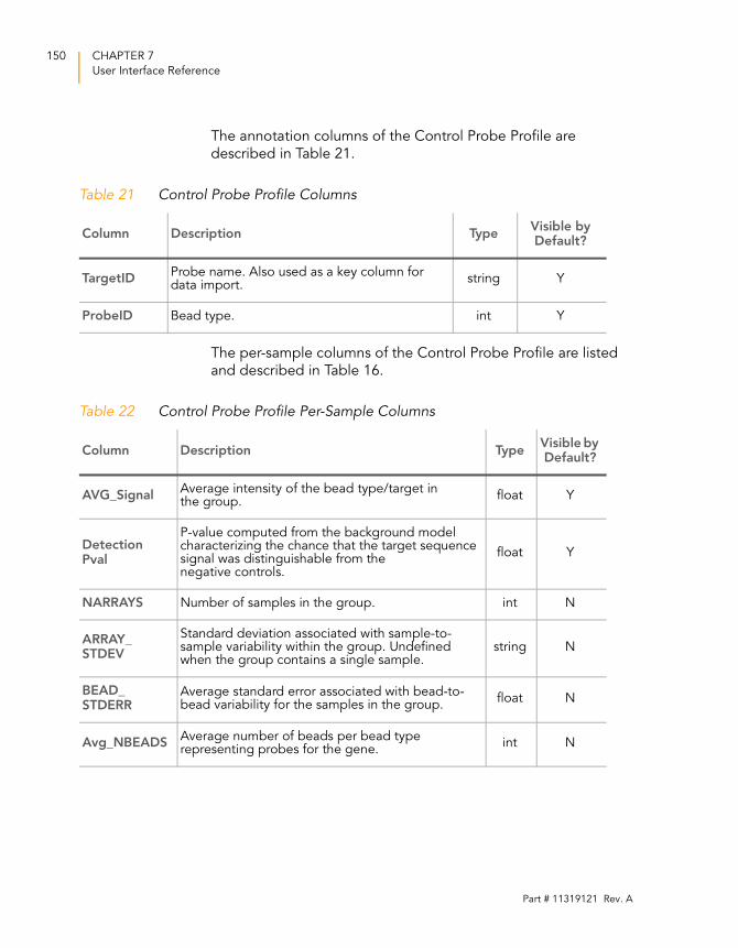
150 CHAPTER 7
User Interface Reference
The annotation columns of the Control Probe Profile are
described in Table 21.
The per-sample columns of the Control Probe Profile are listed
and described in Table 16.
Table 21 Control Probe Profile Columns
Column Description TypeVisible by Default?
TargetIDProbe name. Also used as a key column for data import.
string Y
ProbeID Bead type. int Y
Table 22 Control Probe Profile Per-Sample Columns
Column Description TypeVisible by Default?
AVG_SignalAverage intensity of the bead type/target in the group.
float Y
Detection Pval
P-value computed from the background model characterizing the chance that the target sequence signal was distinguishable from the negative controls.
float Y
NARRAYS Number of samples in the group. int N
ARRAY_STDEV
Standard deviation associated with sample-to-sample variability within the group. Undefined when the group contains a single sample.
string N
BEAD_STDERR
Average standard error associated with bead-to-bead variability for the samples in the group.
float N
Avg_NBEADSAverage number of beads per bead type representing probes for the gene.
int N
Part # 11319121 Rev. A
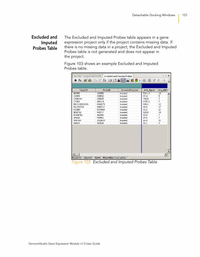
Detachable Docking Windows 151
Excluded andImputed
Probes Table
The Excluded and Imputed Probes table appears in a gene
expression project only if the project contains missing data. If
there is no missing data in a project, the Excluded and Imputed
Probes table is not generated and does not appear in
the project.
Figure 103 shows an example Excluded and Imputed
Probes table.
Figure 103 Excluded and Imputed Probes Table
GenomeStudio Gene Expression Module v1.0 User Guide
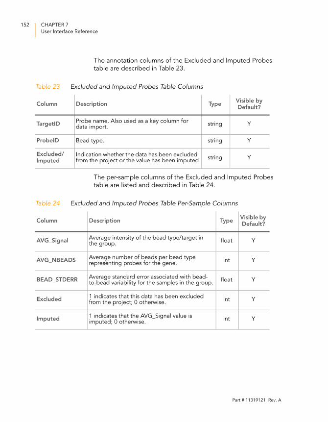
152 CHAPTER 7
User Interface Reference
The annotation columns of the Excluded and Imputed Probes
table are described in Table 23.
The per-sample columns of the Excluded and Imputed Probes
table are listed and described in Table 24.
Table 23 Excluded and Imputed Probes Table Columns
Column Description TypeVisible by Default?
TargetIDProbe name. Also used as a key column for data import.
string Y
ProbeID Bead type. string Y
Excluded/Imputed
Indication whether the data has been excluded from the project or the value has been imputed
string Y
Table 24 Excluded and Imputed Probes Table Per-Sample Columns
Column Description TypeVisible by Default?
AVG_SignalAverage intensity of the bead type/target in the group.
float Y
AVG_NBEADSAverage number of beads per bead type representing probes for the gene.
int Y
BEAD_STDERRAverage standard error associated with bead-to-bead variability for the samples in the group.
float Y
Excluded1 indicates that this data has been excluded from the project; 0 otherwise.
int Y
Imputed1 indicates that the AVG_Signal value is imputed; 0 otherwise.
int Y
Part # 11319121 Rev. A
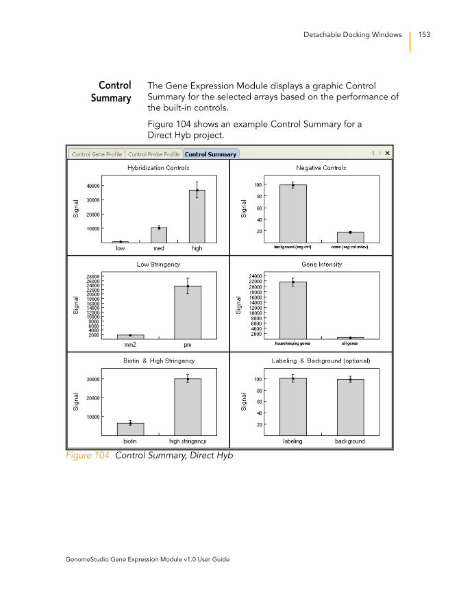
Detachable Docking Windows 153
ControlSummary
The Gene Expression Module displays a graphic Control
Summary for the selected arrays based on the performance of
the built-in controls.
Figure 104 shows an example Control Summary for a
Direct Hyb project.
Figure 104 Control Summary, Direct Hyb
GenomeStudio Gene Expression Module v1.0 User Guide
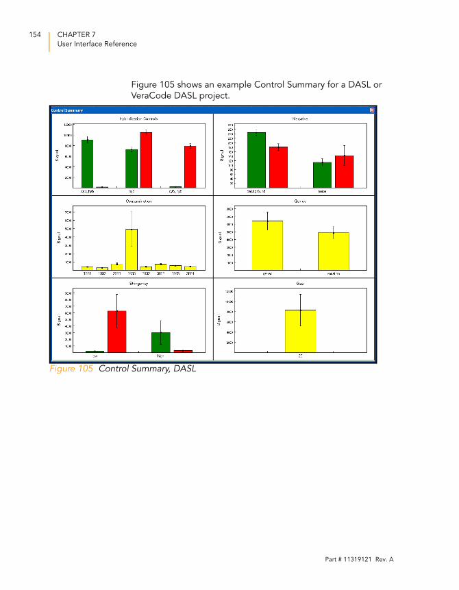
154 CHAPTER 7
User Interface Reference
Figure 105 shows an example Control Summary for a DASL or
VeraCode DASL project.
Figure 105 Control Summary, DASL
Part # 11319121 Rev. A
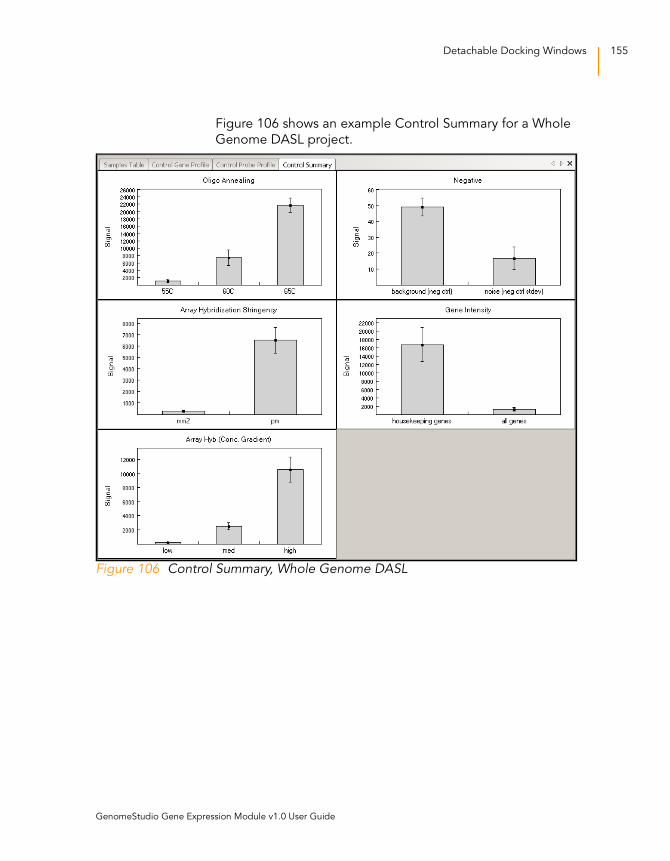
Detachable Docking Windows 155
Figure 106 shows an example Control Summary for a Whole
Genome DASL project.
Figure 106 Control Summary, Whole Genome DASL
GenomeStudio Gene Expression Module v1.0 User Guide
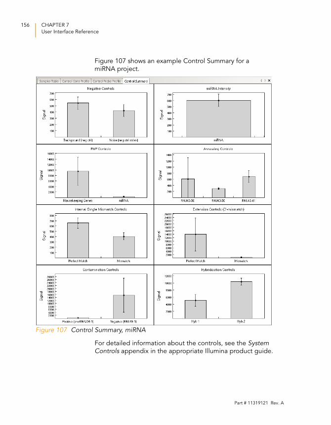
156 CHAPTER 7
User Interface Reference
Figure 107 shows an example Control Summary for a
miRNA project.
Figure 107 Control Summary, miRNA
For detailed information about the controls, see the System Controls appendix in the appropriate Illumina product guide.
Part # 11319121 Rev. A
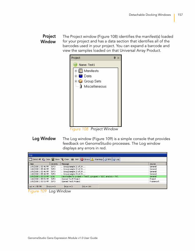
Detachable Docking Windows 157
ProjectWindow
The Project window (Figure 108) identifies the manifest(s) loaded
for your project and has a data section that identifies all of the
barcodes used in your project. You can expand a barcode and
view the samples loaded on that Universal Array Product.
Figure 108 Project Window
Log Window The Log window (Figure 109) is a simple console that provides
feedback on GenomeStudio processes. The Log window
displays any errors in red.
Figure 109 Log Window
GenomeStudio Gene Expression Module v1.0 User Guide
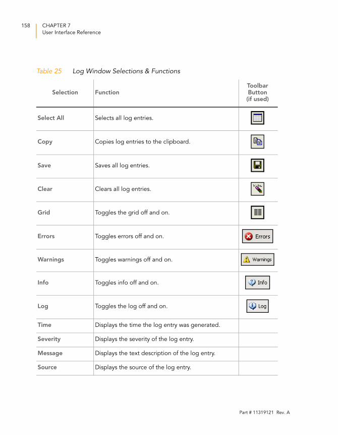
158 CHAPTER 7
User Interface Reference
Table 25 Log Window Selections & Functions
Selection FunctionToolbar Button (if used)
Select All Selects all log entries.
Copy Copies log entries to the clipboard.
Save Saves all log entries.
Clear Clears all log entries.
Grid Toggles the grid off and on.
Errors Toggles errors off and on.
Warnings Toggles warnings off and on.
Info Toggles info off and on.
Log Toggles the log off and on.
Time Displays the time the log entry was generated.
Severity Displays the severity of the log entry.
Message Displays the text description of the log entry.
Source Displays the source of the log entry.
Part # 11319121 Rev. A
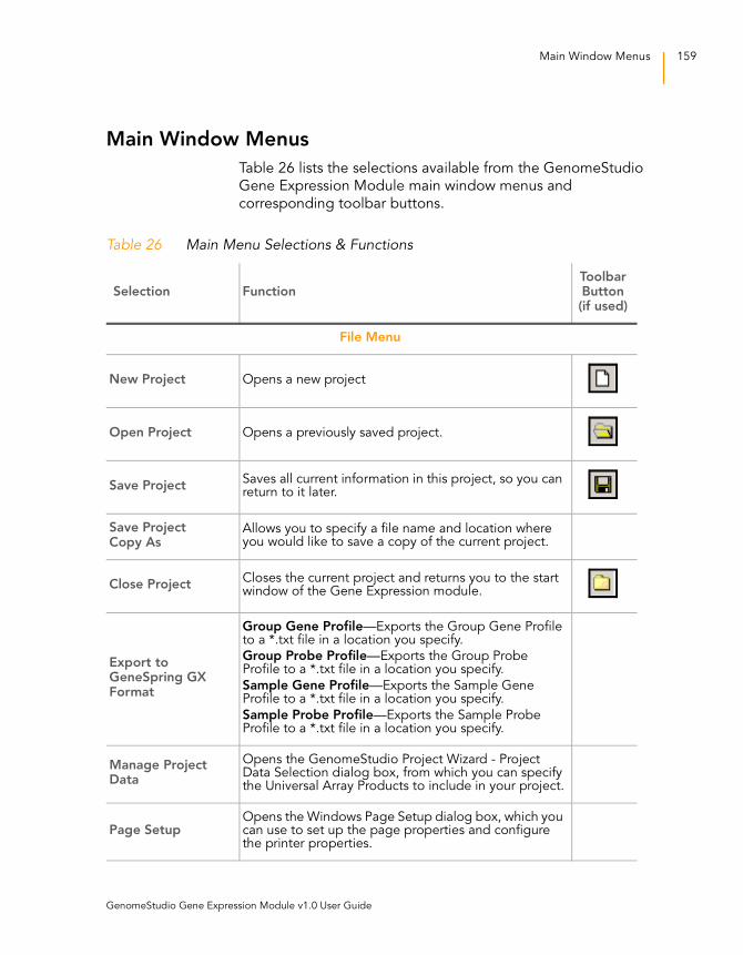
Main Window Menus 159
Main Window Menus
Table 26 lists the selections available from the GenomeStudio
Gene Expression Module main window menus and
corresponding toolbar buttons.
Table 26 Main Menu Selections & Functions
Selection FunctionToolbar Button (if used)
File Menu
New Project Opens a new project
Open Project Opens a previously saved project.
Save ProjectSaves all current information in this project, so you can return to it later.
Save Project Copy As
Allows you to specify a file name and location where you would like to save a copy of the current project.
Close ProjectCloses the current project and returns you to the start window of the Gene Expression module.
Export to GeneSpring GX Format
Group Gene Profile—Exports the Group Gene Profile to a *.txt file in a location you specify.
Group Probe Profile—Exports the Group Probe Profile to a *.txt file in a location you specify.
Sample Gene Profile—Exports the Sample Gene Profile to a *.txt file in a location you specify.
Sample Probe Profile—Exports the Sample Probe Profile to a *.txt file in a location you specify.
Manage Project Data
Opens the GenomeStudio Project Wizard - Project Data Selection dialog box, from which you can specify the Universal Array Products to include in your project.
Page SetupOpens the Windows Page Setup dialog box, which you can use to set up the page properties and configure the printer properties.
GenomeStudio Gene Expression Module v1.0 User Guide
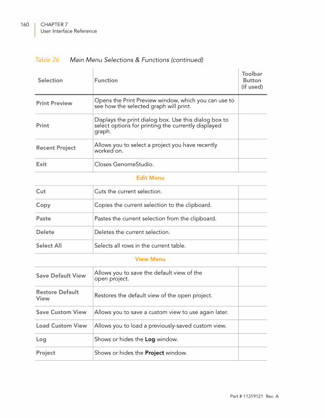
160 CHAPTER 7
User Interface Reference
Print PreviewOpens the Print Preview window, which you can use to see how the selected graph will print.
PrintDisplays the print dialog box. Use this dialog box to select options for printing the currently displayed graph.
Recent ProjectAllows you to select a project you have recently worked on.
Exit Closes GenomeStudio.
Edit Menu
Cut Cuts the current selection.
Copy Copies the current selection to the clipboard.
Paste Pastes the current selection from the clipboard.
Delete Deletes the current selection.
Select All Selects all rows in the current table.
View Menu
Save Default ViewAllows you to save the default view of the open project.
Restore Default View
Restores the default view of the open project.
Save Custom View Allows you to save a custom view to use again later.
Load Custom View Allows you to load a previously-saved custom view.
Log Shows or hides the Log window.
Project Shows or hides the Project window.
Table 26 Main Menu Selections & Functions (continued)
Selection FunctionToolbar Button (if used)
Part # 11319121 Rev. A
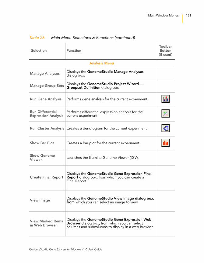
Main Window Menus 161
Analysis Menu
Manage AnalysesDisplays the GenomeStudio Manage Analyses dialog box.
Manage Group SetsDisplays the GenomeStudio Project Wizard—Groupset Definition dialog box.
Run Gene Analysis Performs gene analysis for the current experiment.
Run Differential Expression Analysis
Performs differential expression analysis for the current experiment.
Run Cluster Analysis Creates a dendrogram for the current experiment.
Show Bar Plot Creates a bar plot for the current experiment.
Show Genome Viewer
Launches the Illumina Genome Viewer (IGV).
Create Final ReportDisplays the GenomeStudio Gene Expression Final Report dialog box, from which you can create a Final Report.
View ImageDisplays the GenomeStudio View Image dialog box, from which you can select an image to view.
View Marked Items in Web Browser
Displays the GenomeStudio Gene Expression Web Browser dialog box, from which you can select columns and subcolumns to display in a web browser.
Table 26 Main Menu Selections & Functions (continued)
Selection FunctionToolbar Button (if used)
GenomeStudio Gene Expression Module v1.0 User Guide
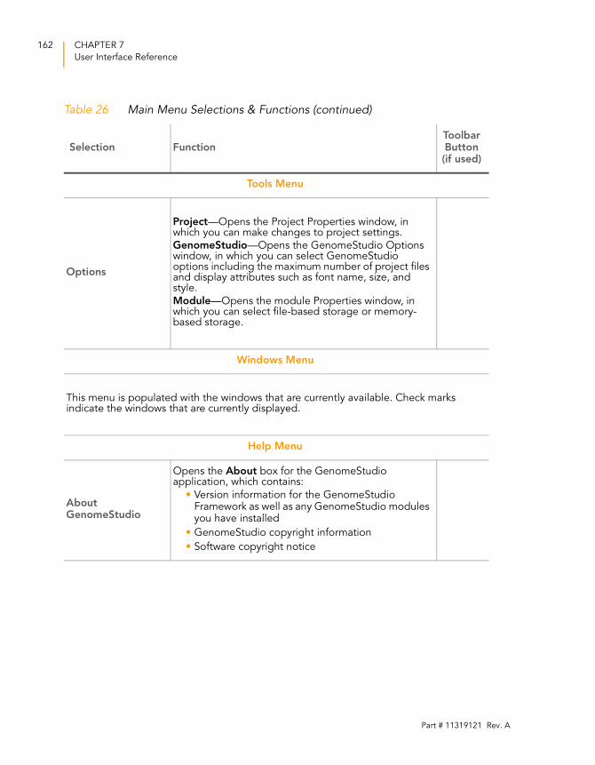
162 CHAPTER 7
User Interface Reference
Tools Menu
Options
Project—Opens the Project Properties window, in which you can make changes to project settings.
GenomeStudio—Opens the GenomeStudio Options window, in which you can select GenomeStudio options including the maximum number of project files and display attributes such as font name, size, and style.
Module—Opens the module Properties window, in which you can select file-based storage or memory-based storage.
Windows Menu
This menu is populated with the windows that are currently available. Check marks indicate the windows that are currently displayed.
Help Menu
About GenomeStudio
Opens the About box for the GenomeStudio application, which contains:
• Version information for the GenomeStudio Framework as well as any GenomeStudio modules you have installed
• GenomeStudio copyright information
• Software copyright notice
Table 26 Main Menu Selections & Functions (continued)
Selection FunctionToolbar Button (if used)
Part # 11319121 Rev. A
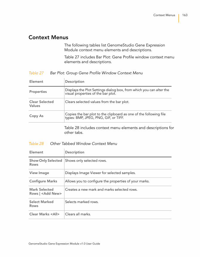
Context Menus 163
Context Menus
The following tables list GenomeStudio Gene Expression
Module context menu elements and descriptions.
Table 27 includes Bar Plot: Gene Profile window context menu
elements and descriptions.
Table 28 includes context menu elements and descriptions for
other tabs.
Table 27 Bar Plot: Group Gene Profile Window Context Menu
Element Description
PropertiesDisplays the Plot Settings dialog box, from which you can alter the visual properties of the bar plot.
Clear Selected Values
Clears selected values from the bar plot.
Copy AsCopies the bar plot to the clipboard as one of the following file types: BMP, JPEG, PNG, GIF, or TIFF.
Table 28 Other Tabbed Window Context Menu
Element Description
Show Only Selected Rows
Shows only selected rows.
View Image Displays Image Viewer for selected samples.
Configure Marks Allows you to configure the properties of your marks.
Mark Selected Rows | <Add New>
Creates a new mark and marks selected rows.
Select Marked Rows
Selects marked rows.
Clear Marks <All> Clears all marks.
GenomeStudio Gene Expression Module v1.0 User Guide
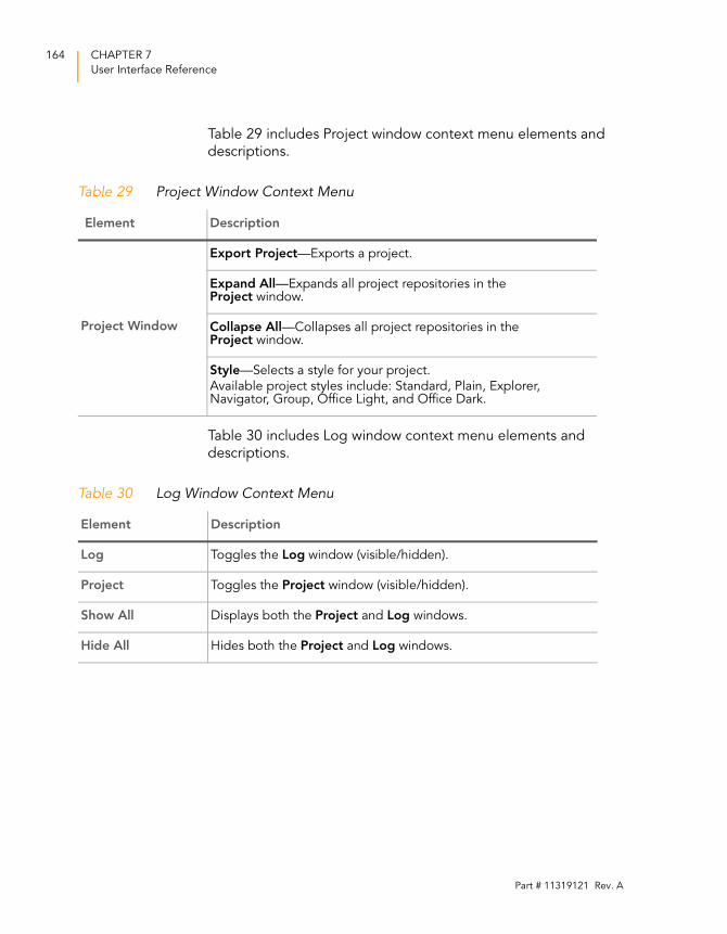
164 CHAPTER 7
User Interface Reference
Table 29 includes Project window context menu elements and
descriptions.
Table 30 includes Log window context menu elements and
descriptions.
Table 29 Project Window Context Menu
Element Description
Project Window
Export Project—Exports a project.
Expand All—Expands all project repositories in the Project window.
Collapse All—Collapses all project repositories in the Project window.
Style—Selects a style for your project.
Available project styles include: Standard, Plain, Explorer, Navigator, Group, Office Light, and Office Dark.
Table 30 Log Window Context Menu
Element Description
Log Toggles the Log window (visible/hidden).
Project Toggles the Project window (visible/hidden).
Show All Displays both the Project and Log windows.
Hide All Hides both the Project and Log windows.
Part # 11319121 Rev. A

Appendix A
Sample Sheet Format
Topics166 Introduction
166 Data Section
168 Sample Sheet Template
168 Sample Sheet Example
GenomeStudio Gene Expression Module v1.0 User Guide
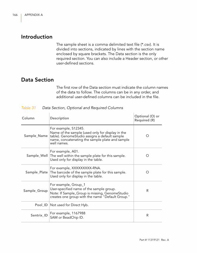
166 APPENDIX A
Introduction
The sample sheet is a comma delimited text file (*.csv). It is
divided into sections, indicated by lines with the section name
enclosed by square brackets. The Data section is the only
required section. You can also include a Header section, or other
user-defined sections.
Data Section
The first row of the Data section must indicate the column names
of the data to follow. The columns can be in any order, and
additional user-defined columns can be included in the file.
Table 31 Data Section, Optional and Required Columns
Column DescriptionOptional (O) or Required (R)
Sample_Name
For example, S12345.
Name of the sample (used only for display in the table). GenomeStudio assigns a default sample name, concatenating the sample plate and sample well names.
O
Sample_Well
For example, A01.
The well within the sample plate for this sample. Used only for display in the table.
O
Sample_PlateFor example, XXXXXXXXX-RNA.
The barcode of the sample plate for this sample. Used only for display in the table.
O
Sample_Group
For example, Group_1
User-specified name of the sample group.
Note: If Sample_Group is missing, GenomeStudio creates one group with the name "Default Group."
R
Pool_ID Not used for Direct Hyb.
Sentrix_IDFor example, 1167988
SAM or BeadChip ID.R
Part # 11319121 Rev. A
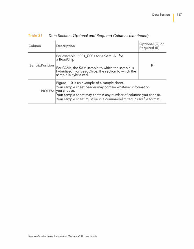
Data Section 167
SentrixPosition
For example, R001_C001 for a SAM, A1 for a BeadChip.
For SAMs, the SAM sample to which the sample is hybridized. For BeadChips, the section to which the sample is hybridized.
R
NOTES:
Figure 110 is an example of a sample sheet.
Your sample sheet header may contain whatever information you choose.
Your sample sheet may contain any number of columns you choose.
Your sample sheet must be in a comma-delimited (*.csv) file format.
Table 31 Data Section, Optional and Required Columns (continued)
Column DescriptionOptional (O) or Required (R)
GenomeStudio Gene Expression Module v1.0 User Guide
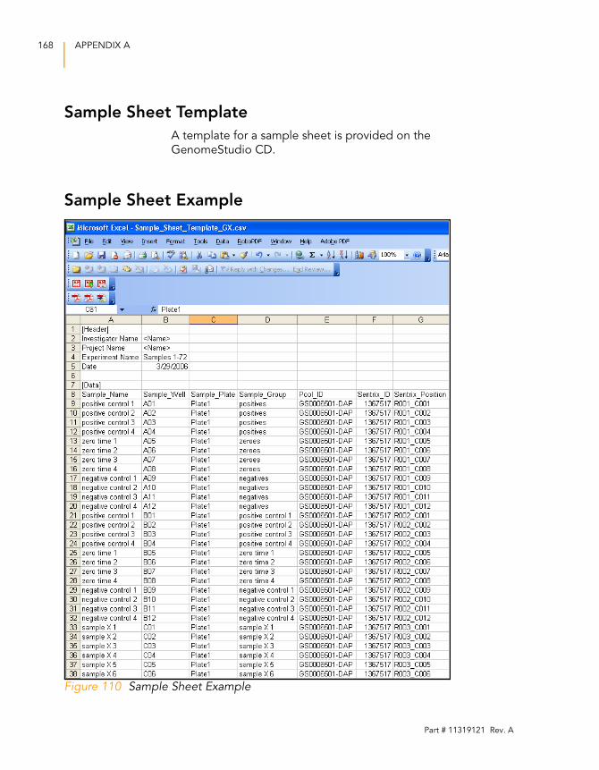
168 APPENDIX A
Sample Sheet Template
A template for a sample sheet is provided on the
GenomeStudio CD.
Sample Sheet Example
Figure 110 Sample Sheet Example
Part # 11319121 Rev. A

Appendix B
Troubleshooting
Introduction
Use this troubleshooting guide to assist you with any questions
you may have about the GenomeStudio Gene Expression
Module.
Frequently Asked Questions
Table 32 lists frequently asked questions and associated
responses.
Table 32 Frequently Asked Questions
# Question Response
1.What is the difference between a group and a groupset?
A group is a collection of arrays combined according to experimental criteria (e.g., arrays hybridized to similar or replicated samples).
A groupset is a collection of groups.
2.What is the minimum statistically-significant detectable fold change of Gene Expression BeadChips?
1.35 fold for single replicates
Much lower for multiple replicates
3.Over what range of intensities can I detect the minimum significant detectable fold change?
The intensity range over which a fold change of ~1.35 are significantly distinguishable is >3 logs.
4.How can I calculate a p-value from the diff score?
p =
1/(10^(diff score/10*(sgn(μcond - μref)))
GenomeStudio Gene Expression Module v1.0 User Guide
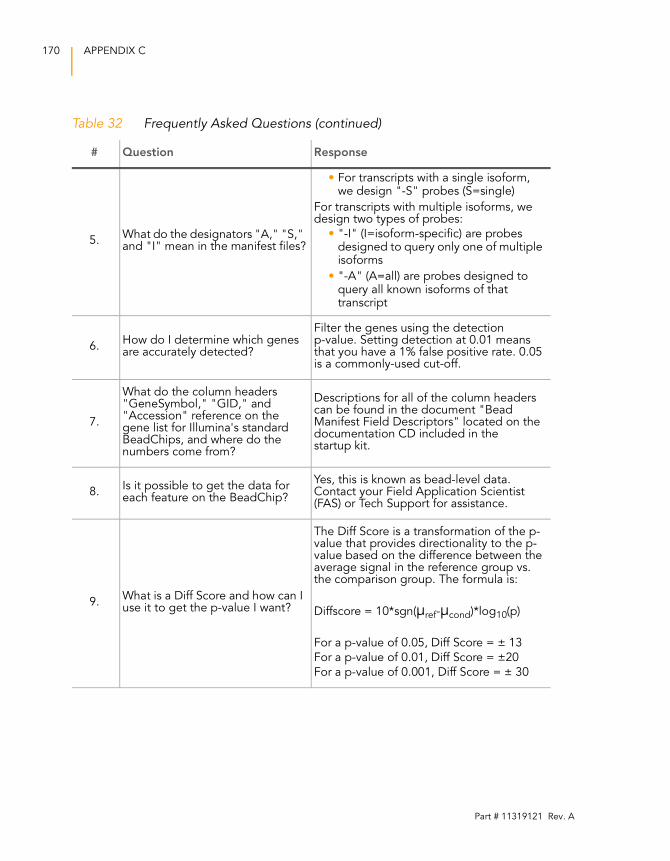
170 APPENDIX C
5.What do the designators "A," "S," and "I" mean in the manifest files?
• For transcripts with a single isoform, we design "-S" probes (S=single)
For transcripts with multiple isoforms, we design two types of probes:
• "-I" (I=isoform-specific) are probes designed to query only one of multiple isoforms
• "-A" (A=all) are probes designed to query all known isoforms of that transcript
6.How do I determine which genes are accurately detected?
Filter the genes using the detection p-value. Setting detection at 0.01 means that you have a 1% false positive rate. 0.05 is a commonly-used cut-off.
7.
What do the column headers "GeneSymbol," "GID," and "Accession" reference on the gene list for Illumina's standard BeadChips, and where do the numbers come from?
Descriptions for all of the column headers can be found in the document "Bead Manifest Field Descriptors" located on the documentation CD included in the startup kit.
8.Is it possible to get the data for each feature on the BeadChip?
Yes, this is known as bead-level data. Contact your Field Application Scientist (FAS) or Tech Support for assistance.
9.What is a Diff Score and how can I use it to get the p-value I want?
The Diff Score is a transformation of the p-value that provides directionality to the p-value based on the difference between the average signal in the reference group vs. the comparison group. The formula is:
Diffscore = 10*sgn(μref-μcond)*log10(p)
For a p-value of 0.05, Diff Score = ± 13
For a p-value of 0.01, Diff Score = ±20
For a p-value of 0.001, Diff Score = ± 30
Table 32 Frequently Asked Questions (continued)
# Question Response
Part # 11319121 Rev. A
Related Documents