Genome Scan Meta-Analysis of Schizophrenia and Bipolar Disorder, Part II: Schizophrenia

Am. J. Hum. Genet. 73:17–33, 2003

17

Genome Scan Meta-Analysis of Schizophrenia and Bipolar Disorder,Part I: Methods and Power AnalysisDouglas F. Levinson,1 Matthew D. Levinson,1 Ricardo Segurado,2 and Cathryn M. Lewis3

1Center for Neurobiology and Behavior, Department of Psychiatry, University of Pennsylvania School of Medicine, Philadelphia; 2Departmentof Genetics, Trinity College, Dublin; and 3Division of Genetics and Development, Guy’s, King’s & St Thomas’ School of Medicine, London

This is the first of three articles on a meta-analysis of genome scans of schizophrenia (SCZ) and bipolar disorder(BPD) that uses the rank-based genome scan meta-analysis (GSMA) method. Here we used simulation to determinethe power of GSMA to detect linkage and to identify thresholds of significance. We simulated replicates resemblingthe SCZ data set (20 scans; 1,208 pedigrees) and two BPD data sets using very narrow (9 scans; 347 pedigrees)and narrow (14 scans; 512 pedigrees) diagnoses. Samples were approximated by sets of affected sibling pairs withincomplete parental data. Genotypes were simulated and nonparametric linkage (NPL) scores computed for 20180-cM chromosomes, each containing six 30-cM bins, with three markers/bin (or two, for some scans). Genomescontained 0, 1, 5, or 10 linked loci, and we assumed relative risk to siblings (lsibs) values of 1.15, 1.2, 1.3, or 1.4.For each replicate, bins were ranked within-study by maximum NPL scores, and the ranks were averaged (Ravg)across scans. Analyses were repeated with weighted ranks ( for each scan). Two P values were�N [genotyped cases]determined for each Ravg: PAvgRnk (the pointwise probability) and Pord (the probability, given the bin’s place in theorder of average ranks). GSMA detected linkage with power comparable to or greater than the underlying NPLscores. Weighting for sample size increased power. When no genomewide significant P values were observed, thepresence of linkage could be inferred from the number of bins with nominally significant PAvgRnk, Pord, or (mostpowerfully) both. The results suggest that GSMA can detect linkage across multiple genome scans.

Introduction

Schizophrenia (SCZ; locus SCZD [MIM #181500]) andbipolar disorder (BPD; loci MAFD1 [MIM 125480] andMAFD2 [MIM 309200]) are severe, common, geneti-cally complex psychiatric phenotypes. As discussed inparts II and III of this series, there have been at least 20SCZ and 22 BPD genome scans to date, with others inprogress. Most twin and family studies suggest that thereare independent genetic factors underlying these disor-ders (Levinson and Mowry 2000), but overlapping fac-tors remain a possibility (Berrettini 2000): severe BPDcases have symptoms resembling SCZ, “schizoaffective”cases with mixed symptoms have increased familial risksof both disorders, and there are chromosomal regionsin which linkage evidence has been reported for bothSCZ and BPD. Most of the available genome scan studieswere initiated early in the 1990s and have been relativelysmall; for SCZ, the average study included ∼60 pedi-grees, and for BPD the average study included 28. Therehave been only one BPD and three SCZ studies reported

Received December 23, 2002; accepted for publication April 9,2003; electronically published June 11, 2003.

Address for correspondence and reprints: Dr. Douglas F. Levinson,Department of Psychiatry, 3535 Market Street, Room 4006, Phila-delphia, PA 19104-3309. E-mail: [email protected]

� 2003 by The American Society of Human Genetics. All rights reserved.0002-9297/2003/7301-0004$15.00

with 1100 pedigrees in the complete scan, although anumber of larger studies are currently in progress.

Although statistically significant findings have beenreported, and some of these have been supported byother studies, there is no locus, for either disorder, thathas consistently produced evidence for linkage in moststudies. It is, therefore, likely that susceptibility is con-ferred by DNA sequence variations at combinations ofloci, each with a small effect on risk (common poly-genes), that the loci of greatest effect vary considerablyacross families and samples (locus heterogeneity), orboth. It may be necessary to combine the results ofmultiple studies to have adequate power to detect theseloci, until much larger samples are available.

The present series of articles uses a rank-based method,genome scan meta-analysis (GSMA) (Wise et al. 1999),to evaluate the evidence for linkage across available SCZand BPD genome scans. This first article briefly reviewsthe theoretical basis for the method and then describesa set of simulation studies that estimate the power ofGSMA to detect linked loci in data sets comparable tothe SCZ and BPD data sets, across a range of geneticmodels, providing empirical standards for assessing sta-tistical significance. The second and third articles thendescribe the GSMAs of SCZ and BPD, respectively (Lewiset al. 2003 [in this issue]; Segurado et al. 2003 [in thisissue]).

18 Am. J. Hum. Genet. 73:17–33, 2003

Several other strategies are available for meta-analysisof linkage data. The most robust approach would be toobtain the original genotypes for each study, construct acombined map of the markers, and perform new linkageanalyses. However, the genotypes are not available forall SCZ and BPD studies and in some cases are restrictedby industry relationships. Construction of a combinedmap has also been problematic, although the new deCodemap (Kong et al. 2002) should make this easier in thefuture. An alternative approach, multiple scan probabil-ity (MSP) (Badner and Gershon 2002b), has been appliedto published SCZ and BPD data (Badner and Gershon2002a). This approach combines P values after correctingfor the size of the linkage area. GSMA and MSP arecompared further below.

GSMA has a number of advantages over other avail-able methods. It requires only placing markers within30-cM bins, rather than determining precise positionalrelationships (although precision in localizing the link-age signal is thereby reduced). Because raw data are notrequired, it is straightforward for investigators to pro-vide the necessary results (linkage scores, P values, orranked data) for each location. When several geneticanalyses have been performed in a particular study, re-sults can be maximized to produce a single set of ranksfor that study. No assumptions are made about modelsof inheritance or of genetic heterogeneity. However,GSMA provides no formal test of genetic hetereoge-neity, and interpretation of genomewide statistical sig-nificance currently relies on empirical grounds.

In contrast to the GSMA, meta-analysis in epidemi-ological studies provides a combined effect size (e.g.,relative risk) with its confidence interval. These methodshave directly interpretable parameter values and allowtesting of heterogeneity between studies, but they re-quire each included study to use the same statisticalanalysis and to test the same hypothesis. Such methodsare difficult to apply to linkage studies, which com-monly report a LOD score (i.e., a measure of signifi-cance) and not an effect size. Their extension to assessevidence of linkage across a region is also not straight-forward. Novel methods for meta-analysis of linkagestudies are therefore needed.

In summary, on the basis of the empirical standardsfor assessing significance reported in this article, theGSMA of SCZ genome scans produced significant ev-idence for linkage for 12–19 of 120 bins, depending onthe approach to assessing significance. By contrast, theGSMA of BPD scans produced no clear statistically sig-nificant evidence for linkage, and the analysis was com-plicated by the many combinations of diagnoses in-cluded in linkage analyses by different studies. The binswith nominally significant P values for BPD showed noclear overlap with the most significant bins for SCZ.Results for each disorder and their implications are dis-

cussed in the second and third articles in this series(Lewis et al. 2003 [in this issue]; Segurado et al. 2003[in this issue]).

Rationale for the Simulation Studies

The simulation studies were intended to clarify thekinds of genetic effects that might be detected by GSMAin the SCZ and BPD data sets. Simplifying assumptionswere necessary, given the unlimited range of possiblegenetic models. GSMA should have the greatest powerto detect effects that are present in a substantial numberof the individual studies (common polygenes) and lesspower to detect effects that are present in very few fam-ilies or samples (extreme locus heterogeneity). We there-fore designed a set of simulation studies based on thecommon polygene model. We recognize that there couldbe susceptibility loci for SCZ and/or BPD that can bedetected only in particular ethnic groups or pedigreestructures. As in all studies of complex disorders, GSMAcan only produce positive evidence for certain effects; itcannot exclude other hypotheses.

There are advantages to using simulated samples ofaffected sibling pairs (ASPs) to model common poly-genes. For families containing a single ASP, if one ignoresdiagnoses in parents or other relatives and if transmis-sion is not recessive (i.e., if risks are similar in sibs, par-ents, and offspring), then there is a straightforward re-lationship between the locus-specific relative risk tosiblings of affected probands (lsibs) and the power todetect linkage for either a single major locus or a mul-tiplicative interaction among loci (James 1971; Risch1987, 1990). Studying samples of ASPs therefore sim-plifies the simulations, because the exact choice of pa-rameter values becomes unimportant as long as theypredict the desired locus-specific lsibs (although, in thereal case, lsibs values can be distorted by imprecise es-timates of population prevalence, particularly for rarerdisorders). A disadvantage of this approach is that ex-tended pedigrees could have greater power under certaingenetic models, but it would have been difficult here toselect a limited yet plausible range of models. Much ofthe linkage information in available SCZ and BPD sam-ples is contained in small nuclear families and, thus, inthe sharing of alleles by ASPs. Therefore, we decided toassess the power of GSMA in samples of families withtwo affected sibs each (independent ASPs). Only dom-inant transmission models were studied, because reces-sive inheritance is unlikely, given the absence of differ-ences between risks to sibs versus risks to parents/offspring for either disorder (Risch 1990) and becauseASPs have less power to detect linkage under dominanttransmission and, thus, results should be conservative.For comparison, recessive inheritance has been studiedfor one of the models at the lowest value of lsibs (1.15),

Levinson et al.: Genome Scan Meta-Analysis: Methods 19

and power was indeed substantially greater than fordominant transmission.

There is a common misconception that ASP analysescannot detect linkage in the presence of genetic heter-ogeneity. For a known risk allele, locus-specific lsibs couldbe computed by genotyping a population-based sampleto establish the risk allele frequency and penetrances andthen determining the relative risk to a carrier probands’sibs, parents, and offspring versus the population risk.In the absence of recessive effects, risks to siblings, par-ents, and offspring will be similar, and, in families trans-mitting the risk allele, ASP identical-by-descent (IBD)allele sharing would be predicted by the locus-specificlsibs: the proportion of ASPs sharing 0 alleles IBD, z0, is

(Risch 1990). However, in linkage studies, the0.25/l sibs

risk locus is unknown, and sharing is measured at nearbymarker loci. If 20% of probands carry an allele thatincreases risk to sibs by threefold, the observed markerz0 will be the weighted average of z0 in the 80% familieswith no linkage (0.25) and in the 20% families withlinkage ( ); thus, populationwide0.25/3 p 0.0833 z p0

, and power will be similar to that for a locus-0.21667specific . Power will bel p 0.25/0.21667 p 1.1538sibs

similarly reduced for nonparametric analyses and forparametric heterogeneity LOD score analyses. Thus, inthe studies presented here, genetic effects are expressedas populationwide lsibs. Results would be similar re-gardless of whether each locus produced a smaller in-crease in risk in many families or a larger increase in asmall proportion of families.

We therefore estimated, for each actual SCZ or BPDgenome scan, the number of ASPs with roughly equivalentlinkage information, as described below. Genotypes weresimulated for large pools of ASP families (two parents ofunknown diagnosis and two affected siblings) on the basisof genetic models predicting specific values of lsibs or nolinkage, and appropriate types and numbers of ASPs wererandomly drawn from the pools of families. Given thelsibs values used here (1.15–1.4), individual samples ineach replicate varied greatly in IBD sharing proportions,as would be observed with either a common polygenemodel or a moderate locus heterogeneity model. Linkageanalyses were performed using nonparametric linkage(NPL) Zall scores (GENEHUNTER 2.0), which correlatehighly with ASP analyses. NPL scores simplified the sim-ulation procedure because, even when multipoint analysesare used (as was the case here), NPL scores maximize atmarker loci rather than between loci, so that only onedata point per marker had to be considered.

Material and Methods

GSMA

GSMA was developed to deal with the diverse studydesigns, analysis methods, and marker densities used in

genome scan studies. GSMA divides the autosomes into120 bins of ∼30 cM in length (X and Y chromosomesare not considered here). The 30-cM bin width is thelargest that divides the smallest chromosomes into twobins each, and it ensures that scores within bins arecorrelated strongly and those between bins more weakly;for the real data sets in the following two articles (Lewiset al. 2003 [in this issue]; Segurado et al. 2003 [in thisissue]), we have assessed the effects of bin placement bycombining adjacent bins, but we have not comprehen-sively studied alternative bin widths. For consistencyacross GSMAs, the boundaries of these bins are definedby Genethon markers, as shown in the following twoarticles (Lewis et al. 2003 [in this issue]; Segurado et al.2003 [in this issue]). Thus, markers located between ∼0cM and 30 cM on chromosome 1 are assigned to bin1.1, those between 30 cM and 60 cM to bin 1.2, etc.To simplify the simulation studies reported here, a 3,600-cM genome was assumed, comprised of 20 180-cM au-tosomes, each containing six bins.

The ranking procedure is illustrated in appendix A.In brief, for each of N studies, the bins are ranked (1 pbest) on the basis of the maximum linkage score or low-est P value observed within each bin. These are within-study ranks (Rstudy). All negative linkage scores are con-sidered equivalent to 0, for consistency with methodsthat produce no negative values—we did not study theinfluence of this “floor” effect on results (i.e., ignoringthe degree of negativity of a score, which could coun-terbalance a very positive score in another study). Forbins with the same maximum scores (such as those with0 scores), each bin is assigned the mean value of theranks in their range. For weighted analyses, each rankis multiplied by the weight for that study—here, thestandardized (see below). Then, the�N (affected cases)average rank (Ravg) is computed for each bin, across allN studies. The mean is 60.5 under the null hypothesis,and values closer to 1 indicate a clustering of evidencefor linkage in that bin. Theoretical thresholds of signif-icance for unweighted analyses are shown in order toprovide the reader with a sense of the relevant rangesof values for different sample sizes. (Note: previousGSMAs reported Rstudy values ranked in descending or-der and summed rather than averaged them. The twoprocedures are statistically identical, but it is more in-tuitive for 1 to be “best.”)

The assessment of statistical significance is summa-rized in the third table of appendix A, in table 1, andin figure 1.

PAvgRnk is the pointwise probability of observing a givenRavg for a bin by chance, in a GSMA of N studies (thirdtable in appendix A). This can be determined theoreti-cally (see appendix B) or by permutation: for a GSMAof N studies, for each permuted replicate, the observed120 Rstudy values for each study are randomly reassigned

20 Am. J. Hum. Genet. 73:17–33, 2003

to bins and then averaged across studies for each bin.At least 5,000 replicates are produced, or a larger num-ber to produce stable estimates of small or marginalP values. If the observed Ravg is �38.9, then PAvgRnk isthe proportion of bins in the random replicates with

(e.g., among 120 bins # 5,000 replicates).R p 38.9avg

Pord (short for “PAvgRnkForder”) is the probability of ob-serving a given Ravg for a bin by chance in bins with thesame “place” in the ascending order of Ravg values inrandomly permuted replicates (table 1; fig. 1). Thus, inthe permutation test described above, the Ravg values foreach replicate are now sorted by size. If the observedfourth-best , Pord is the probability of ob-R p 31.0avg

serving a value �31.0 in the 5,000 fourth-place bins inthe replicates. Consider the analogy of a race: PAvgRnk

determines which bins are the “fastest runners,” whereasPord determines whether it is a “fast race” (i.e., whetherthe top finishers all ran faster than the top finishers inmost races). As shown by the simulation studies reportedbelow, it is this aggregate information about the set ofmost significant bins that provides additional informa-tion about linkage when genomewide significance is notobserved for PAvgRnk.

PAvgRnk and Pord have been computed as (r � 1)/(n �, where r is the number of replicates exceeding a par-1)

ticular score and n is the total number of replicates. Asexplained by North et al. (2002, p. 439), “if the nullhypothesis is true, then the test statistics of the n rep-licates and the test statistic of the actual data are allrealizations of the same random variable,” and thus theP value is more accurate when the data set being testedis included in the ranking of all known outcomes. LikePAvgRnk, Pord is a pointwise value—∼5% of bins will have

in unlinked replicates, although these valuesP � .05ord

will be scattered throughout both large and small ranks.The 5% threshold for genomewide significance of eachtype of P value must therefore be corrected for 120 bins:

. This is larger than the threshold of.05/120 p .000417pointwise for linkage results (Lander andP p .00002Kruglyak 1995), because, for GSMA, inference is re-stricted to discrete bins of 30 cM. Statistical propertiesof Pord, including nonindependence of the values, arediscussed further below.

The terminology described above is summarized inappendix C.

Description of the Samples

The simulated GSMA data sets were based on threeof the SCZ and BPD data sets described in the secondand third papers in this series, respectively.

1. The simulated SCZ data sets (table 2) approximatedthe linkage information of the 20 genome scan anal-yses from 17 independent projects included in theSCZ GSMA, using narrow diagnoses (usually SCZ

plus schizoaffective disorders). Simulated samplesizes were the reported number of ASPs in a cor-responding study or an estimate based on a mul-ticenter SCZ sample (Levinson et al. 2000), where(N[genotyped cases] � N[informative pedigrees]) ≈

. The proportion of1.39 # (N[independent ASPs])genotyped parents was as reported or was estimatedfrom study descriptions and was increased whenmany unaffected relatives were genotyped. Averagemarker spacing was 10 or 15 cM, similar to thecorresponding study.

2. The simulated BPD data sets resembled sets of ge-nome scans in the BPD GSMA. These studies con-sidered various diagnostic combinations of bipolar-I, bipolar-II, schizoaffective disorder–bipolar type,recurrent major depression, and sometimes otherdiagnoses. Thus, the number of affected cases andinformative families varied according to the model.The simulated data sets resembled those for the twonarrowest models considered in the BPD GSMA:the BP-VN (very narrow) data set (table 3) includesnine simulated samples whose sizes resemble thoseof the nine BPD scans analyzed under a very narrowdiagnostic model, considering only BPI and SAB asaffected; the BP-N (narrow) data set (table 4) in-cludes 14 simulated samples whose sizes resemblethose of the 14 BPD scans analyzed under a narrowmodel, considering BPI, SAB, and BPII cases as af-fected. Numbers of ASPs were determined as forSCZ, with zero, one, or two genotyped parents eachin ∼33% of families, on the basis of the SCZ data(because pedigree structure details were sometimesunavailable). Average marker spacing was 10 cM.

Simulation Procedure

Genotypes were created by simulation for chromo-somes with either no linked locus, or with one linkeddisease locus under one of four dominant genetic mod-els:

1. [ , ,l p 1.15 q(D) p 0.434 f(dd) p 0.01sibs

];f(Dd,DD) p 0.12. [ , ,l p 1.2 q(D) p 0.0169 f(dd) p 0.006sibs

];f(Dd,DD) p 0.033. [ , ,l p 1.3 q(D) p 0.0173 f(dd) p 0.005sibs

];f(Dd,DD) p 0.034. [ , ,l p 1.4 q(D) p 0.0244 f(dd) p 0.004sibs

];f(Dd,DD) p 0.025where D indicates the disease allele, d the wild-type al-lele, q the allele frequency, and f the penetrance. Thisrange of values was selected because samples of 500–1,000 ASPs have been shown to have reasonable powerto detect linkage at values ∼1.3–1.4, with power in-creasing rapidly above this range and decreasing rapidlybelow it (Hauser et al. 1996).

Levinson et al.: Genome Scan Meta-Analysis: Methods 21

Table 1

P Values Based on Ordered Average Ranks (Pord)

BIN

OBSERVED

Ravga PAvgRnk

RANDOMLY PERMUTED REPLICATESb

Pordc

Ravg

Replicate1

Ravg

Replicate2 …

Ravg

Replicate5,000 Mean Ravg � SD

1st Place 30.3 .00006 35.8 41.1 … 36.6 39.2 � 3.1 .01042nd Place 31.5 .00015 38.5 43.0 … 42.4 42.0 � 2.3 .00023rd Place 34.2 .00044 40.8 43.4 … 45.0 43.6 � 1.9 .00024th Place 34.3 .00045 40.9 44.0 … 45.5 44.7 � 1.7 .0002

… … … … … … … … …120th Place 82.2 .99 83.1 77.2 79.1 81.5 � 3.0 1.0

a Weighted Ravg values for one GSMA replicate (20 studies, 10 disease loci, ; ed2md8 in table 5),l p 1.15sibs

sorted with the first-place (“best”) bin at the bottom of the column.b Rstudy values were randomly reassigned into columns, and Ravg was computed for each bin of each replicate

and then sorted. Means and SDs describe the Ravg distributions for 1st-place, 2nd-place, etc., bins with no linkage.c “By chance, how frequently would the average rank for a bin in the same place be as low as or lower than

the observed average rank?” , where r is the number of randomly permuted replicates forP p (r � 1)/(n � 1)ord

which the Ravg of the jth-place bin is less than or equal to the observed jth-place Ravg, and n is the number ofreplicates (North et al. 2002). See figure 1 for illustration.

Figure 1 Determining Pord: observed and expected ordered Ravg values. The black line shows the 120 observed Ravg values, sorted withthe first-place bin on the right. The light gray line and vertical error bars show the mean � 2 SD of the jth-place bin from 5,000 randompermutations. In the absence of linkage, Ravg values lower than the expected distribution are observed infrequently throughout the genome.With linkage, they are clustered among the highest values of Ravg, as shown here. As shown in table 1, Pord is the probability of observing agiven value of Ravg (black line) by chance, given its place in the order of observed Ravg values, which is determined from the distribution ofordered Ravg values (light gray line and error bars).

To confirm that power would be greater for reces-sive transmission, a single set of replicates was createdfor the SCZ data set as discussed below, using pa-rameter values predicting [ ,l p 1.15 q(D) p 0.276sibs

, ].f(dd,Dd) p 0.01 f(DD) p 0.04LINKAGE-format files were created with sets of fam-

ilies with two parents of unknown diagnosis and twoaffected offspring. Simulated genotypes were created us-ing GENSIM (Kruglyak et al. 1996; Kruglyak and Daly1998). The structure of the simulated chromosomes isshown in figure 2. Each chromosome was 180 cM long(six 30-cM bins). Bins contained three markers (10-cM

spacing), except for four SCZ scans with 15-cM spacing.Disease loci were conservatively placed halfway betweenadjacent markers, given that many other aspects of theprocedure were idealized (e.g., identical marker maps inall studies, no genotyping errors).

Four types of genomes were created (table 5), with 1,5, or 10 linked loci in “edge” or “mid” bins. Lowermultipoint NPL scores were anticipated near the edgesof chromosomes because of reduced information con-tent. The value of lsibs was constant for all disease lociin a simulated genome. Sets of “linked” chromosomesfor 10,000 families were created for each of 24 com-

22 Am. J. Hum. Genet. 73:17–33, 2003

Table 2

SCZ Simulated Data Set

SAMPLE

ACTUAL STUDY SIMULATION STUDYa

NO. OF ASP FAMILIES

WITH N GENOTYPED

PARENTS

No. ofPedigrees

No. ofCases Weight

MapDensity

(cM)No. ofASPs N p 2 N p 1 N p 0

1 294 669 2.3165 10 330 135 115 802 185 390 1.7687 10 240 85 80 753 71 171 1.1711 10 90 85 5 04 81 170 1.1677 15 90 0 0 905 77 179 1.1982 15 75 12 19 446 67 164 1.1469 15 75 12 19 447 74 169 1.1643 15 75 12 19 448 54 146 1.0822 10 55 32 19 49 60 132 1.0290 10 72 15 25 3010 43 126 1.0053 10 57 30 19 811 53 113 .9520 10 60 10 25 2512 43 96 .8775 10 56 15 23 1813 30 79 .7960 10 45 4 27 1414 22 79 .7960 10 65 20 30 1515 21 58 .6821 10 40 32 4 416 13 56 .6702 10 50 20 20 1017 1 43 .5873 10 50 5 25 2018 5 37 .5448 10 40 15 15 1019 9 35 .5298 10 30 15 9 620 5 33 .5145 10 30 16 8 6

Total 1,208 2,945 20.0000 1,625 570 506 547

a Numbers of pedigrees and genotyped affected cases are those in the actual study (see thesecond article in this series [Lewis et al. 2003 {in this issue}]). Number of ASPs (simulationstudy) was assigned as described in the text. Weight p , where� �( N[cases])/mean( N[cases])“cases” p number of genotyped affected cases in the actual study (see text).

binations of four values of lsibs, two marker densities,and zero, one, or two parents genotyped. “Unlinked”sets of chromosomes for 100,000 families were createdfor each of six combinations of two marker densitiesand zero, one, or two parents genotyped. NPL analysiswas performed for each family, and tables of NPL scoresat each marker locus were stored for each family tocreate pools from which samples were then drawn.

For each GSMA replicate, a row of NPL scores for asingle chromosome was selected randomly from the tablewith the appropriate lsibs, marker density, number of par-ents typed, and chromosome type (linked-edge, linked-mid, or unlinked), for each chromosome for each familyin each individual scan in each data set, for each full model(lsibs, and numbers of linked/edge, linked/mid, and un-linked chromosomes) (table 5). For example, for one ofthe 100 “ed1” model (see footnote “a” of table 5 for anexplanation of model abbreviations) SCZ GSMA repli-cates with , for sample 1, NPL scores for onel p 1.15sibs

linked/edge chromosome and 19 unlinked chromosomeswere drawn from the appropriate pools for each of 135ASP families with two typed parents, 115 with one typedparent, and 80 with no typed parents, and so on for theother 19 SCZ samples, totalling 1,625 pedigrees with 570,

506, and 547 families with two, one, and zero parentstyped, respectively (table 2). Within each data set, the NPLscores within each scan were combined across families( ), and the maximum NPL scores�� [NPL]/ N[pedigrees]within the 120 bins for each sample were saved in a table,substituting 0 for negative scores. These scores wereranked across the 120 bins, averaging the ranks of setsof tied bins. The original analyses considered Rstudy valuesin descending order and sums of ranks. Here we presentequivalent values in ascending order and average ranksas noted above. Simulations were performed with 100replicates for each linked model and 1,000 replicates ofunlinked data sets (no linkage present).

Weighting Procedure

Rstudy values were weighted for some analyses. Alter-native weights were tested on 100 SCZ replicates(ed1md4/1.15). The total NPL score was computed foreach marker, extrapolating the values for bins containingtwo markers ( , and , andM3 p M2 M2 p [M1 � M2]/2)the best score was selected for each bin. Pearson’s cor-relation coefficient (r and R2) was computed between eachbin’s NPL score and either the unweighted or weighted

Levinson et al.: Genome Scan Meta-Analysis: Methods 23

Table 3

BP-VN Simulated Data Set

SAMPLE

ACTUAL STUDY

SIMULATION

STUDYa

NO. OF ASP FAMILIES

WITH N GENOTYPED

PARENTS

No. ofPedigrees

No. ofCases Weight

No. ofASPs N p 2 N p 1 N p 0

1 2 24 .527 18 6 6 62 7 27 .559 17 6 6 53 15 41 .689 22 7 7 84 13 40 .681 23 8 8 75 5 42 .698 31 10 10 116 41 107 1.114 55 18 18 197 39 115 1.155 63 21 21 218 97 264 1.749 139 46 46 479 128 288 1.827 133 44 44 45

Total 347 948 9.000 501 166 166 169

a Numbers of pedigrees and genotyped affected cases are those in the actualstudy (see the third article in this series [Segurado et al. 2003 {in this issue}]). Seethe table 2 footnote and the text for details.

Ravg, comparing three weights: (a) , (b)N(pedigrees), or (c) . The average� �N(pedigrees) N(genotyped cases)

R2 values were 0.79 (unweighted), 0.778 (a), 0.856 (b),and 0.856 (c). Because (b) would excessively downweightstudies with large pedigrees, was�N(genotyped cases)adopted here. We used N from the actual correspondingstudy, because a GSMA will generally include sampleswith varying pedigree structures, so that the weight is arough approximation of relative linkage information.

Statistical Analyses

Values of PAvgRnk were computed as described above(and see appendix A, table 1 and fig. 1). For weightedanalyses, P values computed by permutation were com-pared with the actual probability of observing a givenvalue or one more extreme in the 1,000 unlinked rep-licates, and results agreed quite closely. For example, forSCZ, the 5% threshold was 46.815 by the permutationprocedure and 46.715 based on unlinked replicates.

For Pord, a new procedure was developed. Pord valuesare pointwise measures—that is, when numbers from 1to 120 were placed randomly in each of 20 rows (similarto the grids of values for 120 bins for the 20 SCZ sam-ples) and averaged, 4.69% of bins had . How-P ! .05ord

ever, 5.74% of bins met this criterion in 250 unlinkedSCZ data sets. We noted that edge bins 1 and 6 hadlarger (worse) average ranks (61.68 vs. 59.91 for bins1–4; for bin 1 vs. bin 4, 999 df, )t p 8.47 P ! .00001(shown in fig. 3) and slightly higher mean Pord values(.51065 vs. .50245; ; for bin 1 vs.t p 2.53 P p .011bin 4, chromosome 1), as predicted from the lower link-age information content at the ends of maps. Thus, thesmaller (better) Ravg of a middle bin would be evaluatedagainst the distribution of middle � edge bins, lowering

its PAvgRnk. When rows were permuted by chromosomerather than by bin, mean Pord values for edge versusmiddle bins were .506972 and .503461 ( [nott p 0.032significant] for bin 1 vs. bin 4). Therefore, the analysesreported below used permutation by chromosome tocompute Pord. However, this method (adapted for chro-mosomes of nonuniform lengths) was not more conser-vative in the SCZ and BPD GSMAs in the articles thatfollow and was not used. Presumably, this phenomenonis more apparent in idealized simulated data.

Distributions of PAvgRnk and Pord were compared in rep-licates containing linked loci versus the unlinked repli-cates, to determine how false and true positive resultscould best be differentiated.

Results

Detection of Significant Linkage with NPL Scoresversus GSMA

Table 6 shows the proportion of linked bins achievinggenomewide suggestive or nominal significance levels forweighted PAvgRnk or NPL scores, for SCZ data sets( or 1.3). GSMA was as powerful as NPLl p 1.15sibs

and more powerful for weaker linkage, owing in partto the fact that GSMA considers 30-cM bins so thatthere is a more modest correction for multiple testing.Figure 4 shows mean numbers of bins achieving ge-nomewide significance ( ), us-P p .05/120 p .0004167ing empirical thresholds from 1,000 unlinked replicates(120,000 bins) per data set, for weighted ranks. In con-trast to table 6, where only the disease locus bins areconsidered and mid and edge bins are considered sep-arately, in figure 4 the total number of genomewide sig-nificant values is shown, ∼20% of which are in bins

24 Am. J. Hum. Genet. 73:17–33, 2003

Table 4

BP-N Simulated Data Set

SAMPLE

ACTUAL STUDY

SIMULATION

STUDYa

NO. OF ASP FAMILIES

WITH N GENOTYPED

PARENTS

No. ofPedigrees

No. ofCases Weight

No. ofASPs N p 2 N p 1 N p 0

1 2 24 .481 18 6 6 62 7 39 .614 27 9 9 93 7 36 .589 24 8 8 84 15 46 .666 26 9 9 85 13 44 .652 26 9 9 86 20 48 .681 23 8 8 77 5 42 .637 31 10 10 118 22 118 1.067 80 27 27 269 41 107 1.016 55 18 18 1910 39 208 1.417 141 47 47 4711 51 128 1.112 64 21 21 2212 65 232 1.496 139 46 46 4713 97 336 1.801 199 66 66 6714 128 325 1.771 164 55 55 54

Total 512 1,733 14.000 1,017 339 339 339

a See the table 2 footnote and the text for details.

adjacent to disease bins. Power was excellent to detectat least one such value for SCZ and BP-N data sets ifthe populationwide locus-specific lsibs was at least 1.3.When , SCZ data sets had good power whenl p 1.15sibs

�5 loci were linked, as did BP-N when 10 loci werelinked. Power was poor for BP-VN.

Power to Detect Nominally Significant PAvgRnk

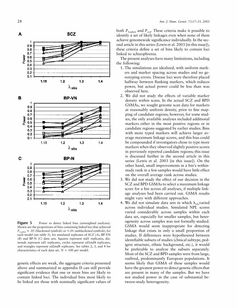
Power to detect PAvgRnk at the 95% and 99% thresh-olds is shown in figure 5A–C. Unweighted results areshown to demonstrate power in the absence of otherassumptions, such as weighting schemes. For compari-son, table 7 summarizes power for weighted analyses forselected models, typically ∼3%–7% greater. The dataare illustrated in figure 6. Power at the 95% thresholdwas high for SCZ data sets (20 samples; 1,625 ASPs);low for BP-VN data sets (nine studies; 501 ASPs), exceptat the high lsibs; and intermediate for BP-N (14 studies,1,017 ASPs). A limitation of GSMA is also illustrated:for weaker genetic effects, as the number of linked lociincreases, the power to detect each individual locus de-clines, but there can be considerable power to detect atleast some of the linked loci. Note that analyses pre-sented below consider only lsibs values of 1.15 and 1.3,which are sufficiently representative.

Aggregate Significance Thresholds

One can also consider aggregate thresholds of signif-icance: does the number or pattern of bins achieving acriterion exceed chance expectation? For PAvgRnk, in thethree sets of 1,000 unlinked GSMA replicates, only 5%

of data sets had �11 bins with . This canP ! .05AvgRnk

be considered as a criterion for concluding that linkageis present somewhere in the genome, although this doesnot determine which bins are the true positives.

Pord is a type of order statistic analysis. The P valuesof sequential order statistics are not independent. LetX[r] be the rth order statistic for the set of average ranks(Ravg)—that is, X[r] has the value of the rth-lowest av-erage rank, and, specifically, the value X[1] is the lowestaverage rank. If X[r] has a very low Pord, there is anincreased probability that the next-most-extreme orderstatistic, X[ ], will also be significant, sincer � 1 X[r �

, by definition, and X[ ] therefore has a1] ! X[r] r � 1truncated distribution. The dependency can be deter-mined theoretically by using the distribution functionfor summed ranks (Wise et al. 1999; appendix B), butit is difficult to compute theoretically the more generalprobability of observing a cluster of N significant Pord

values. Empirically, we found that only 5% of unlinkedreplicates had four or more Pord values !.05 out of the10 lowest Ravg values. This is a second empirical thresh-old for determining, in aggregate, whether there is evi-dence of linkage in a GSMA.

The Relationship between Pord and PAvgRnk Values

The most striking difference between replicates withand without linked chromosomes was the pattern ofPord and PAvgRnk values. Table 7 shows the number ofbins with , , or both, for selectedP ! .05 P ! .05AvgRnk ord

data sets. These data are shown graphically in figure6, for data sets, to illustrate the followingl p 1.15sibs

findings:

Levinson et al.: Genome Scan Meta-Analysis: Methods 25

Figure 2 Marker maps for simulation studies. Genotypes were simulated for 180-cM chromosomes, on each of which six 30-cM bins(segments) were structured as shown. Marker locations are M1, M2, M3. For the SCZ data sets, some studies had 10-cM marker spacing (A)and others had 15-cM spacing (B); all BP data sets were simulated with 10 cM spacing. Linked (disease) and unlinked (nondisease) chromosomeswere created (C). Disease loci (indicated by “D”) were located midway between two markers, either in the first (edge) or third (middle) bin.Genomes consisted of 20 chromosomes (120 bins); see table 5 for structures of genomes.

1. As the number of linked bins and the genetic effectand power increase, more bins have both PAvgRnk

and Pord values !.05, versus a mean of ∼0.55 binswith these values in unlinked data sets. This is trueeven when , where linkage is difficultl p 1.15sibs

to detect (Hauser et al. 1996); for example, for SCZdata sets, with 5–10 disease loci, PAvgRnk and Pord

are !.05 for many disease and adjacent bins.2. As power and number of linked loci increase, fewer

bins have only but not . TheP ! .05 P ! .05AvgRnk ord

number of bins with only is relatively con-P ! .05ord

stant, except that the number increases for adjacentbins when there are more linked chromosomes—anobservation that may be relevant to interpreting thedata for the SCZ GSMA in the next article in thisseries (Lewis et al. 2003 [in this issue]).

3. When multiple bins have both PAvgRnk and P !ord

, many or most of them contain linked loci, even.05when genetic effects are too weak to produce asignificant PAvgRnk for each bin. For example, forthe SCZ replicates with 10 linked loci (l psibs

; ed2md8), an average of almost 11 linked and1.15adjacent bins had PAvgRnk and , comparedP ! .05ord

with slightly more than 1 unlinked bin (table7)—that is, 190% were linked or adjacent. Forunlinked data sets, !5% of GSMA replicates con-tain four or more such bins for SCZ or BP-N, or

five or more bins for the smaller BP-VN data sets.Therefore, conservatively, observing five or morebins with PAvgRnk and is a genomewideP ! .05ord

criterion that suggests linkage in some or all ofthese bins.

4. By contrast, when there is only a single linked locusin the genome, only the magnitude and not the pat-tern of PAvgRnk and Pord values can identify linkage.

Combined P Values

Finally, we considered the possibility of a test for thesignificance of a pair of PAvgRnk and Pord values (Pcomb).These values are not independent and cannot be com-bined theoretically. One can determine, from unlinkedreplicates, the frequency of values more extreme than agiven pair; however, if this is done for several pairs, thetype I error rate becomes inflated rapidly. For example,if one restricts values to [ and ],P ! .05 P ! .05AvgRnk ord

then, for each PAvgRnk, there is a maximum Pord such that. If one plots all such pairs on a log scale,P ! .000417comb

however, one defines a triangle within which lies 0.001of all observed pairs of values in unlinked SCZ data sets.There is an infinite number of ways to further restrictthis space to reduce type I error, so any one choice wouldbe arbitrary. In practice, a criterion of [ andP ! .05AvgRnk

] selects 0.005 of bins in unlinked replicates,P ! .05ord

26 Am. J. Hum. Genet. 73:17–33, 2003

Table 5

Types of Genomes Created in the Simulation Studies

MODELa

NO. OF CHROMOSOMES WITH

NO. OF

GSMAREPLICATES

Disease Locusin Bin 1(“Edge”)

Disease Locusin Bin 3(“Mid”)

No DiseaseLocus

(“Unlinked”)

For each lsibs value:ed1 1 0 19 100md1 0 1 19 100ed1md4 1 4 15 100ed2md8 2 8 10 100

Unlinked 0 0 20 1,000

a ed1 p 1 linked/edge chromosome; md1 p 1 linked/mid chromosome; ed1md4 p1 linked/edge and 4 linked/chromosomes; ed2md8 p 1 linked/edge and 8 linked/midchromosomes. For each data set (SCZ, BP-VN, BP-N), 100 complete GSMA replicateswere created from the appropriate pools of simulated linked and unlinked chromosomes(20 chromosomes per individual study for each replicate) for each value of lsibs (1.15,1.2, 1.3, and 1.4) for each model; and 1,000 replicates for each data set with no linkage.Weighted analyses were carried out for each data set for and 1.3 and forl p 1.15sibs

the unlinked replicates.

Figure 3 Mean average rank by bin for unlinked replicates. Shown are the means � SD of the average ranks of each bin (over allchromosomes) in the 1,000 unlinked replicates of the SCZ data set. “Edge” bins (1 and 6) have lower summed ranks than “mid” bins (2–5).This contributed to an inflated type I error rate when Pord values were computed by permuting the order of ranks in each study by bin, andwas corrected by permuting by chromosome so that summed ranks of edge and middle bins were compared with their own distributions.

and this criterion performs adequately in detecting link-age. For example, in 100 replicates of SCZ ed2md8 datasets ( ), 65% of disease bins, 23.4% of ad-l p 1.15sibs

jacent bins, 2.2% of other bins on linked chromosomes,and 1% of bins on unlinked chromosomes had PAvgRnk

and ; the proportions of each of these types ofP ! .05ord

bins within the Pcomb triangle described above were58.9%, 38.3%, 2%, and 0.9%. Thus, pending furtherstudy, Pcomb does not define significance for individualbins. When multiple bins are associated with PAvgRnk and

, these bins are the most likely to contain linkedP ! .05ord

loci.

Recessive Transmission

To confirm that, for simple ASP families, power wouldbe greater than reported here for recessive transmissionmodels, 100 SCZ replicates were simulated under therecessive model described above, predicting l psibs

. Each genome contained 5 linked chromosomes (to1.15

Levinson et al.: Genome Scan Meta-Analysis: Methods 27

Table 6

Power of NPL Analysis versus GSMA (SCZ Data Set)

POWER

Genomewide Significance Suggestive Linkage (once/scan) Nominal (Pointwise Significance)

P ! .000417AvgRnk

NPL� 4.2

P ! .0083AvgRnk

NPL� 3.09

P ! .05AvgRnk

BIN AND

l VALUE

1 LinkedBin

5 LinkedBins

10 LinkedBins

1 LinkedBin

5 LinkedBins

10 LinkedBins

1 LinkedBin

5 LinkedBins

10 LinkedBins

Mid bins:lsibs p 1.15 .22 .22 .16 .03 .62 .58 .50 .34 .82 .85 .79lsibs p 1.3 .84 .73 .58 .47 .98 .96 .90 .92 1.00 .99 .98

Edge bins:lsibs p 1.15 .16 .17 .14 .02 .64 .55 .39 .23 .84 .81 .69lsibs p 1.3 .63 .55 .34 .24 .89 .97 .72 .76 1.00 .89 .93

NOTE.—Shown for the SCZ data set are the proportion of linked bins whose weighted PAvgRnk values or maximum NPL scores met criteriafor genomewide significance ( [.05/120]; NPL 4.2), suggestive linkage ( [1/120]; NPL 3.09), or pointwiseP ! .000417 P ! .00833AvgRnk AvgRnk

significance ( ). For NPL, power is the average across all linked/edge or linked/mid bins for all models with that lsibs.P ! .05AvgRnk

Figure 4 Mean number of bins per replicate achieving genomewide significance. Shown is the mean number of bins (in 100 replicatesper model) with (the threshold for genomewide significance p .05/120), for weighted analyses. Diamonds represent SCZ dataP � .0004167sets, squares represent BP-N data sets, and circles represent BP-VN data sets. Blackened symbols represent data for , unblackenedl p 1.3sibs

symbols represent data for .l p 1.15sibs

simplify the simulation, all were linked/edge) and 15unlinked chromosomes. The power to detect a givenlinked bin was 0.94 for , 0.79 for , andP ! .05 P ! .00830.39 for , considerably greater than that ob-P ! .000417served for dominant transmission and (tablel p 1.15sibs

6). The mean number of bins with PAvgRnk and P !ord

was 9.48, compared with !6 for dominant trans-.05mission (fig. 6).

Discussion

A rank-based method, GSMA, can have considerablepower to detect genetic linkage for the models studied

here. Power has been studied for PAvgRnk, the probabilityof observing a bin’s average rank by chance; Pord, theprobability of observing the jth-place bin’s average rankin jth-place bins in randomly permuted data; and theco-occurrence of nominally significant values for bothmeasures. For , even the smallest data set (BP-l � 1.3sibs

N) had good/excellent power to detect at least nominallysignificant PAvgRnk. Genomewide significance can be iden-tified in larger data sets by a PAvgRnk corrected for multipletesting ( ). GSMA had power comparable toP ! .000417or greater than that of the NPL scores from which theranked data were derived, although with greatly reducedlocalization of the linkage signal. Where populationwide

28 Am. J. Hum. Genet. 73:17–33, 2003

Figure 5 Power to detect linked bins (unweighted analyses).Shown are the proportions of bins containing linked loci that achieved

(blackened symbols) or �.01 (unblackened symbols), forP � .05AvgRnk

each model (see table 5), for simulated replicates of SCZ (A), BP-VN(B) and BP-N (C) data sets. Squares represent md1 replicates, dia-monds represent ed1 replicates, circles represent ed1md4 replicates,and triangles represent ed2md8 replicates. See tables 2, 3, and 4 forcharacteristics of each data set. per model.N p 100

genetic effects are weak, the aggregate criteria presentedabove and summarized in appendix D can still providesignificant evidence that one or more bins are likely tocontain linked loci. The individual bins most likely tobe linked are those with nominally significant values of

both PAvgRnk and Pord. These criteria make it possible toidentify a set of likely linkages even when none of themachieve genomewide significance individually. In the sec-ond article in this series (Lewis et al. 2003 [in this issue]),these criteria define a set of bins likely to contain locilinked to schizophrenia.

The present analyses have many limitations, includingthe following:

1. The simulations are idealized, with uniform mark-ers and marker spacing across studies and no ge-notyping errors. Disease loci were therefore placedhalfway between flanking markers, which reducespower, but actual power could be less than wasobserved here.

2. We did not study the effects of variable markerdensity within scans. In the actual SCZ and BPDGSMAs, we sought genome scan data for markersat reasonably uniform density, prior to fine map-ping of candidate regions; however, for some stud-ies, the only available analyses included additionalmarkers either in the most positive regions or incandidate regions suggested by earlier studies. Binswith more typed markers will achieve larger av-erage maximum linkage scores, and this bias couldbe compounded if investigators chose to type moremarkers when they observed slightly positive scoresin previously reported candidate regions; this issueis discussed further in the second article in thisseries (Lewis et al. 2003 [in this issue]). On theother hand, small improvements in a bin’s within-study rank in a few samples would have little effecton the overall average rank across studies.

3. We did not study the effect of our decision in theSCZ and BPD GSMAs to select a maximum linkagescore for a bin across all analyses, if multiple link-age analyses had been carried out. GSMA resultsmight vary with different approaches.

4. We did not simulate data sets in which lsibsvariedacross individual studies. Simulated NPL scoresvaried considerably across samples within eachdata set, especially for smaller samples, but heter-ogeneity across samples was not formally studied.GSMA would seem inappropriate for detectinglinkage that exists in only a small proportion ofstudies. If differences were hypothesized betweenidentifiable subsets of studies (clinical subtype, ped-igree structure, ethnic background, etc.), it wouldbe preferable to analyze the subsets separately.Most of the SCZ and BPD samples were from large,outbred, predominantly European populations. Itseems likely that GSMA of these samples wouldhave the greatest power to detect genetic effects thatare present in many of the samples. But we havenot studied power in the case of substantial be-tween-study heterogeneity.

Levinson et al.: Genome Scan Meta-Analysis: Methods 29

Table 7

Relationship between PAvgRnk and Pord: Mean Numbers of Disease, Adjacent and Unlinked Bins with PAvgRnk! .05, Pord ! .05, or Both

DATA SET

AND NO.OF LINKED

LOCI

MEAN

POWER

( )P ! .05AvgRnk

MEAN NO.OF BINS

WITH

P ! .05AvgRnk

MEAN NO. OF BINS

WITH PAvgRnk AND P ! .05ord

MEAN NO. OF BINS

WITH ONLY P ! .05AvgRnk

MEAN NO. OF BINS

WITH ONLY P ! .05ord

Disease Adjacent Unlinked Disease Adjacent Unlinked Disease Adjacent Unlinked

lsibsp 1.15:BP-VN:

1 .59 6.84 .10 .12 1.01 .49 .53 4.59 .03 .10 4.515 .47 8.01 .62 .52 1.13 1.71 1.22 2.81 .31 .63 4.4910 .40 8.99 1.53 1.13 .72 2.50 1.76 1.35 .78 1.35 3.07

BP-N:1 .85 7.00 .28 .24 1.23 .57 .53 4.15 .01 .09 5.385 .71 9.29 2.08 1.79 1.80 1.48 1.05 1.08 .28 .63 3.6910 .62 12.51 4.68 3.53 1.41 1.56 .91 .42 1.10 2.41 3.86

SCZ:1 .82 6.67 .31 .37 1.25 .51 .46 3.77 .01 .05 4.785 .84 10.50 3.21 2.70 1.98 1.00 .70 .91 .18 .90 3.9110 .76 13.91 6.50 4.21 1.29 1.14 .59 .18 .81 2.91 3.85

lsibs p 1.3:BP-VN:

1 .80 6.44 .29 .26 .68 .51 .49 4.21 .02 .08 4.165 .70 9.53 2.04 1.76 1.82 1.48 1.01 1.42 .25 .49 3.4010 .63 12.54 4.54 3.38 1.66 1.71 .78 .47 1.21 3.05 5.18

BP-N:1 .96 7.20 .55 .54 1.47 .41 .65 3.58 .00 .02 4.265 .92 11.53 4.25 3.84 2.23 .36 .48 .37 .09 .82 3.8010 .86 16.36 8.43 6.19 1.49 .20 .02 .03 .85 4.35 5.29

SCZ:1 1.00 7.02 .87 .97 1.77 .13 .49 2.79 .00 .03 3.225 .99 13.25 4.91 5.52 2.60 .03 .11 .08 .02 .93 4.2710 .97 18.65 9.65 7.99 .98 .01 .01 .01 .25 4.21 3.88

Unlinked:BP-VN:

0 6.00 .58 5.42 5.49SCZ:

0 6.00 .51 5.48 5.46

NOTE.—Power is the mean probability of observing weighted for each linked bin. Disease bins are those containing a linked locus, adjacentP ! .05AvgRnk

bins are those adjacent to a linked bin, and all other bins are considered unlinked.

5. Other issues not considered here include the powerto detect linkage when lsibs varies across loci in thesame genome, the effect of two or more disease lociin the same bin or on the same chromosome, re-cessive transmission models, and X- or Y-chro-mosome linkage.

There may be advantages to other approaches tometa-analysis. The best approach would presumably beto perform new analyses using genotypes from eachstudy. For example, several schizophrenia candidateregions have been studied by large multicenter collab-orations that genotyped a common set of markers andcombined the samples for analysis (Gill et al. 1996;SLCG 1996; Levinson et al. 2000). However, these stud-ies included only a subset of collaborating SCZ linkagesamples and did not scan the genome. Dorr et al. (1997)has suggested a logistic regression approach for ana-lyzing allele sharing in multiple samples while takingpossible heterogeneity across samples into account. Thismethod was applied by Levinson et al. (2000), but ap-plying it to all samples would require access to rawgenotypes from all studies, which was not possible here.

Badner and Gershon (2002b) developed the MSPmethod for meta-analysis of candidate regions and ap-plied it to SCZ and BPD (Badner and Gershon 2002a).MSP identifies clusters of positive values from the actualdata and assesses significance using P values correctedfor the size of the region. Similarities and differences inthe GSMA and MSP analyses of SCZ and BPD are dis-cussed in the following two articles (Lewis et al. 2003[in this issue]; Segurado et al. 2003 [in this issue]). Wewould note here that it could be problematic to combinethe lowest P values from genome scans, which, partic-ularly for smaller scans, can be severely upwardly biased(Goring et al. 2001). However, the relative power ofthese methods is not yet clear. For example, perhaps bygiving full weight to very low P values, MSP could betterdetect linkage in the presence of substantial heteroge-neity across samples. GSMA might be more powerfulwhen small genetic effects were present in all samples.

In conclusion, simulation studies suggest that GSMAcan identify regions of the genome that are likely tocontain linked loci, if the size of the data set is appro-priate to the magnitude of the genetic effect. While the

30 Am. J. Hum. Genet. 73:17–33, 2003

Figure 6 Number of loci with nominally significant PAvgRnk, Pord, or both. Data from table 7 are shown for the BP-VN (9 studies) andSCZ (20 studies) data sets weighted analysis, with Pord computed by permuting by chromosome, for . Blackened bars represent meanl p 1.15sibs

number of bins with both values !.05, diagonally striped bars represent bins with only , and white bars represent bins with onlyP ! .05AvgRnk

. Sets of bars are labeled by data set (BP or SCZ) and the number of linked loci in the data set (1 p md1, 5 p ed1md4, and 10 pP ! .05ord

ed2md8). Shown are the number of bins with these values for disease � adjacent bins (left-most six sets of bars), bins on chromosomes containingno disease locus (next six sets), and bins in completely unlinked data sets (the average of BP-VN-unlinked and SCZ-unlinked, which werevirtually identical). See text for details.

method has excellent power under some circumstancesto detect genomewide significant linkage, GSMA couldprove most useful when there are many weakly linkedloci. In these cases, there may be more nominally sig-nificant bins than expected by chance, including an ex-cess of bins with nominally significant P values both forthe average rank and for the average rank given theorder of ranks. No method can exclude linkage in anychromosomal region for a complex disorder, and GSMAdata should not be interpreted in this way; however,where direct computation of linkage scores from rawgenotypes is not feasible, GSMA provides a useful firststep toward evaluating whether data from multiple ge-

nome scans provide evidence for linkage in specific chro-mosomal regions.

Acknowledgments

The late Dr. Lodewijk Sandkuijl originally suggested de-signing a power analysis of GSMA. His thoughtful advice onthis and many other issues will be greatly missed. Dr. KennethKendler and Mr. Michael Levinson provided helpful sugges-tions about communicating these ideas more clearly. Dr. SevillaDetera-Wadleigh’s role in organizing the bipolar meta-analysisprovided the impetus to include those samples in the simulationstudy. This work was supported by National Institute of Men-tal Health grants MH61602 and K24-MH64197 (to D.F.L).

Levinson et al.: Genome Scan Meta-Analysis: Methods 31

Appendix A

Summary of GSMA Ranking Procedure: Rstudy, Ravg, and PAvgRnk

First, select the most significant linkage score in each bin for each study (0 if negative):

STUDY

MAXIMUM LINKAGE SCORE IN BIN

1.1 1.2 1.3 1.4 … 22.2

1 .83 .41 1.90 3.19 … .322 0 0 0 .22 … .89

… … … … … … …9 .37 .44 .78 1.44 … .66

Within each study, rank each score (Rstudy) from 1 (“best”) to 120 (“worst”), with ties (e.g., for study 2, 38 binsincluding bins 1, 2, and 3 had 0 scores, leading to a rank of 101.5 for each).

STUDY

WITHIN-STUDY RANK (Rstudy) FOR BIN

1.1 1.2 1.3 1.4 … 22.2

1 45 69 9 1 … 922 101.5 101.5 101.5 87 … 33

… … … … … … …9 93 87.5 59 9 … 58

Then compute the average rank (Ravg) for each bin across studies. Each Rstudy can be multiplied by a weightingfactor before averaging (e.g., the standardized ). Compute pointwise PAvgRnk (probability of the�N[affected cases]average rank) for each bin (theoretically, or empirically if weighted) to answer the question “By chance, howfrequently would any bin have Ravg this low or lower?”

STUDY WEIGHT

WEIGHTED WITHIN-STUDY RANK FOR BIN

1.1 1.2 1.3 1.4 … 22.2

1 2.1 94.5 144.9 18.9 2.1 … 193.23 .9 91.35 91.35 91.35 78.3 … 29.7

… … … … … … …9 .5 46.5 43.75 29.5 4.5 … 29

Ravg 82.6 88.9 46.3 26.1 … 50.1Empirical PAvgRnk .9630 .9916 .1350 .0025 .2102

Thresholds of significance for Ravg are shown below for GSMAs with different numbers of studies (computedtheoretically for unweighted analyses; empirical weighted thresholds will vary slightly).

NO. OF

STUDIES

Ravg THRESHOLD FOR

PAvgRnk p

.05 .01 .001

9 41.44 34.0 26.2214 45.29 39.14 32.5720 47.75 42.6 36.95

32 Am. J. Hum. Genet. 73:17–33, 2003

Appendix B

Summed Rank Distribution Function

The GSMA procedure is based on an understanding of the distribution of summed ranks across multiple sets ofranked data, with within-study bins ranked in descending order (Wise et al. 1999). Under the null hypothesis ofno linkage in a bin, the ranks will be randomly assigned from each study. The distribution function is

m

P X p R p 0 , for R ! m ;�( )iip1

d1 R � kn � 1 mk( )p �1 , for m � R � nm ;� ( ) ( )m m � 1 kn kp0

p 0 , for R 1 nm ,

where R is summed rank, Xi is the rank of study i, m is the number of studies, n is the number of bins (120), andd is the integer part of . For unweighted analyses, pointwise P values for R can be determined directly(R � m)/nfrom this distribution, although, for weighted analyses, a permutation procedure is required, as described above.

It is mathematically equivalent to rank bins in descending order and to average rather than sum the ranks acrossbins. For any R, the equivalent average ascending rank Ravg is: . Results have been expressed this(n � 1) � (R/m)way in the current article to provide a more intuitive terminology.

Appendix C

Summary of Terminology

Bin: One of 120 30-cM autosomal segments used asunits of analysis in GSMA; bin 2.1 is the first 30 cM ofchromosome 2.

Rstudy (within-study rank): The rank of each bin withina single study, based on the maximum linkage score (orlowest P value) within it. The bin containing the bestscore has a rank of 1. All negative and 0 scores areconsidered to be tied. For weighted analyses, each rawrank is multiplied by the study’s weighting factor.

Ravg (average rank): The average of a bin’s within-study ranks or weighted ranks across all studies.

PAvgRnk (probability of Ravg): The pointwise probabilityof observing a given Ravg for a bin in a GSMA of Nstudies, determined by theoretical distribution (un-weighted analysis only) or by permutation test (fig. 2).

Pord (probability of Ravg given the order): The pointwiseprobability that, for example, a 1st-place, 2nd-place,3rd-place, etc., bin would achieve Ravg at least this ex-treme in a GSMA of N studies.

Genomewide significance: For , correctiona p 0.05for 120 bins yields a threshold for genome-wide signif-icance of .000417 for PAvgRnk or Pord. For suggestive link-age (a result observed once per scan by chance), a p

.1/120 p 0.0083

Appendix D

Criteria for Genomewide Significance

For individual bins, the criterion for genomewide sig-nificance is . When linkage is likely toP ! .000417AvgRnk

be present in one or more bins, the aggregate criteriaare as follows: �11 bins with , �4 binsP ! .000417AvgRnk

with among the 10 best values of Ravg, or �5P ! .05ord

bins with and . Bins withP ! .05 P ! .05AvgRnk ord

and are most likely to containP ! .05 P ! .05AvgRnk ord

linked loci. No valid combined significance criterion wasidentified.

Electronic-Database Information

The URL for data presented herein is as follows:

Online Mendelian Inheritance in Man (OMIM), http://www.ncbi.nlm.nih.gov/Omim/ (for SCZD, MAFD1, and MAFD2)

References

——— (2002a) Meta-analysis of whole-genome linkage scansof bipolar disorder and schizophrenia. Mol Psychiatry 7:405–411

Badner JA, Gershon ES (2002b) Regional meta-analysis ofpublished data supports linkage of autism with markers onchromosome 7. Mol Psychiatry 7:56–66

Berrettini WH (2000) Are schizophrenic and bipolar disordersrelated? A review of family and molecular studies. Biol Psy-chiatry 48:531–538

Levinson et al.: Genome Scan Meta-Analysis: Methods 33

Dorr D, Rice J, Armstrong C, Reich T, Blehar M (1997) Ameta-analysis of chromosome 18 linkage data for bipolarillness. Genet Epidemiol 14:617–622

Gill M, Vallada H, Collier D, Sham P, Holmans P, Murray R,McGuffin P, et al (1996) A combined analysis of D22S278marker alleles in affected sib-pairs: support for a suscepti-bility locus for schizophrenia at chromosome 22q12. Schizo-phrenia Collaborative Linkage Group (Chromosome 22).Am J Med Genet 67:40–45

Goring HHH, Terwilliger JD, Blangero J (2001) Large upwardbias in estimation of locus-specific effects from genome-widescans. Am J Hum Genet 69:1357–1369

Hauser ER, Boehnke M, Guo SW, Risch N (1996) Affectedsib-pair interval mapping and exclusion for complex genetictraits: sampling considerations. Genet Epidemiol 13:117–138

James JW (1971) Frequency in relatives for an all-or-none trait.Ann Hum Genet 35:47–49

Kong A, Gudbjartsson DF, Sainz J, Jonsdottir GM, Gudjons-son SA, Richardsson B, Sigurdardottir S, Barnard J, Hall-beck B, Masson G, Shlien A, Palsson ST, Frigge ML, Thor-geirsson TE, Gulcher JR, Stefansson K (2002) Ahigh-resolution recombination map of the human genome.Nat Genet 31:241–247

Kruglyak L, Daly M (1998) Linkage thresholds for two-stagegenome scans. Am J Hum Genet 62:994–996

Kruglyak L, Daly MJ, Reeve-Daly MP, Lander ES (1996) Par-ametric and nonparametric linkage analysis: a unified mul-tipoint approach. Am J Hum Genet 58:1347–1363

Lander E, Kruglyak L (1995) Genetic dissection of complextraits: guidelines for interpreting and reporting linkage re-sults. Nat Genet 11:241–247

Levinson DF, Holmans P, Straub RE, Owen MJ, Wildenauer

DB, Gejman PV, Pulver AE, Laurent C, Kendler KS, WalshD, Norton N, Williams NM, Schwab SG, Lerer B, MowryBJ, Sanders AR, Antonarakis SE, Blouin JL, DeLeuze JF,Mallet J (2000) Multicenter linkage study of schizophreniacandidate regions on chromosomes 5q, 6q, 10p, and 13q:schizophrenia linkage collaborative group III. Am J HumGenet 67:652–663

Levinson DF, Mowry BJ (2000) Genetics of schizophrenia. In:Pfaff DW, Berrettini WH, Maxson SC, Joh TH (eds) Geneticinfluences on neural and behavioral functions. CRC Press,New York, pp 47–82

Lewis CM, Levinson DF, Wise LH, DeLisi LE, Straub RE,Hovatta I, Williams NM, et al (2003) Genome scan meta-analysis of schizophrenia and bipolor disorder, part II:schizophrenia. Am J Hum Genet 73:34–48 (in this issue)

North BV, Curtis D, Sham PC (2002) A note on the calculationof empirical P values from Monte Carlo procedures. Am JHum Genet 71:439–441

Risch N (1987) Assessing the role of HLA-linked and unlinkeddeterminants of disease. Am J Hum Genet 40:1–14

——— (1990) Linkage strategies for genetically complextraits. I. Multilocus models. Am J Hum Genet 46:222–228

Schizophrenia Linkage Collaborative Group for Chromosomes3, 6 and 8 (1996) Additional support for schizophrenia link-age on chromosomes 6 and 8: a multicenter study. Am JMed Genet 67:580–594

Segurado R, Detera-Wadleigh SD, Levinson DF, Lewis CM,Gill M, Nurnberger JI Jr, Craddock N (2003) Genome scanmeta-analysis of schizophrenia and bipolar disorder, part III:bipolar disorder. Am J Hum Genet 73:49–62 (in this issue)

Wise LH, Lanchbury JS, Lewis CM (1999) Meta-analysis ofgenome searches. Ann Hum Genet 63:263–272