Genetic Structure of Britons

ARTICLEdoi:10.1038/nature14230

The fine-scale genetic structure of theBritish populationStephen Leslie1,2,3*, Bruce Winney3*, Garrett Hellenthal4*, Dan Davison5, Abdelhamid Boumertit3, Tammy Day3,Katarzyna Hutnik3, Ellen C. Royrvik3, Barry Cunliffe6, Wellcome Trust Case Control Consortium 2{,International Multiple Sclerosis Genetics Consortium{, Daniel J. Lawson7, Daniel Falush8, Colin Freeman9, Matti Pirinen10,Simon Myers11, Mark Robinson12, Peter Donnelly9,111 & Walter Bodmer31

Fine-scale genetic variation between human populations is interesting as a signature of historical demographic eventsand because of its potential for confounding disease studies. We use haplotype-based statistical methods to analysegenome-wide single nucleotide polymorphism (SNP) data from a carefully chosen geographically diverse sample of2,039 individuals from the United Kingdom. This reveals a rich and detailed pattern of genetic differentiation withremarkable concordance between genetic clusters and geography. The regional genetic differentiation and differingpatterns of shared ancestry with 6,209 individuals from across Europe carry clear signals of historical demographicevents. We estimate the genetic contribution to southeastern England from Anglo-Saxon migrations to be under half,and identify the regions not carrying genetic material from these migrations. We suggest significant pre-Roman butpost-Mesolithic movement into southeastern England from continental Europe, and show that in non-Saxon parts ofthe United Kingdom, there exist genetically differentiated subgroups rather than a general ‘Celtic’ population.

The genetic composition of human populations varies throughout theworld, as a result of the interplay between population movement, admix-ture, natural selection and genetic drift. Characterizing such geograph-ical population structure provides insights into demographic historyand is critical to genetic studies of disease1–3.

Human population structure is reasonably well understood at broadscales, for example between and within continents4–10. Here we invest-igate structure over much finer scales, in Caucasians within the UnitedKingdom (UK) consisting of England, Scotland, Wales and NorthernIreland. We use ‘Britain’ (technically Great Britain) to refer to the singleisland consisting of modern-day England, Scotland and Wales. UK popu-lation structure has been studied before, typically on relatively small sam-ples using various single-locus systems and recently genome-wide SNPdata11,12. These earlier studies show some regional variation at particularloci, with a weak, roughly north–south cline in allele frequencies genome-wide, suggesting that population structure in the UK is rather limited.

Samples and analysisTo investigate fine-scale population structure in the UK, and to pro-vide well-characterized controls for disease studies, we assembled asample, the People of the British Isles (PoBI) collection, as previouslydescribed13. Our analyses used 2,039 PoBI samples from rural areaswithin the UK, genotyped as part of the Wellcome Trust Case Consor-tium 2 (WTCCC2), who had all four grandparents born within 80 kmof each other. We thus effectively sample DNA from the grandparents.The grandparents’ average year of birth was 1885 (s.d. 18 years). Asthe DNA from each PoBI participant is a random sample of theirgrandparents’ DNA, our approach allows investigation of fine-scale

population structure in rural areas of the UK before the major popu-lation movements of the twentieth century.

To provide context for the UK samples, we analysed 6,209 samplesfrom 10 countries in continental Europe genotyped in the WTCCC2study of multiple sclerosis14. To ensure compatibility between the PoBIand continental European samples we restricted attention to autoso-mal SNPs genotyped in both samples (approximately 500,000 SNPs,see Methods).

Fine-scale UK population differentiationConsistent with earlier studies of the UK, population structure withinthe PoBI collection is very limited. The average of the pairwise FST esti-mates between each of the 30 sample collection districts is 0.0007, witha maximum of 0.003 (Supplementary Table 1).

Against this background of very limited structure within the UK,we applied a recently developed method for detecting fine-scale popu-lation structure, fineSTRUCTURE15, to the PoBI samples, to look formore subtle effects. See Methods (also Extended Data Figs 1 and 2) foran informal description, details, interpretation under both discrete andisolation-by-distance models, assessment of convergence, and enhance-ments to the algorithm as applied in this study. In contrast to commonlyused approaches such as principal components or ADMIXTURE16,fineSTRUCTURE explicitly models the correlation between nearby SNPsand uses extended multi-marker haplotypes throughout the genome.This substantially increases its power to detect subtle levels of geneticdifferentiation.

The fineSTRUCTURE algorithm can divide samples into geneticclusters hierarchically, from coarser to finer levels of structuring. We

*These authors contributed equally to this work.

{Information about participants appears in the Supplementary Information.1These authors jointly supervised this work.

1Murdoch Childrens Research Institute, Royal Children’s Hospital, Flemington Road, Parkville, Victoria 3052, Australia. 2University of Melbourne, Department of Mathematics and Statistics, Parkville,Victoria 3010, Australia. 3University of Oxford, Department of Oncology, Old Road Campus Research Building, Roosevelt Drive, Oxford OX3 7DQ, UK. 4University College London Genetics Institute, DarwinBuilding, Gower Street, London WC1E 6BT, UK. 5Counsyl, 180 Kimball Way, South San Francisco, California 94080, USA. 6University of Oxford, Institute of Archaeology, 36 Beaumont Street, Oxford OX12PG, UK. 7University of Bristol, Department of Mathematics, University Walk, Bristol BS8 1TW, UK. 8College of Medicine, Swansea University, Singleton Park, Swansea SA2 8PP, UK. 9The Wellcome TrustCentre for Human Genetics, Roosevelt Drive, Oxford OX3 7BN, UK. 10University of Helsinki, P.O. Box 20, Helsinki, FI-00014, Finland. 11University of Oxford, Department of Statistics, 1 South Parks Road,Oxford OX1 3TG, UK. 12University of Oxford, University Museum of Natural History, Parks Road, Oxford OX1 3PW, UK.

1 9 M A R C H 2 0 1 5 | V O L 5 1 9 | N A T U R E | 3 0 9

Macmillan Publishers Limited. All rights reserved©2015

applied fineSTRUCTURE to the PoBI samples’ genetic data withoutreference to the known geographical locations. The genetic clusteringcan be assessed with respect to geography by plotting individuals on amap of the UK (at the centroid of their grandparents’ places of birth)and examining the inferred genetic clusters, for different levels of thehierarchical clustering.

Figure 1 shows this map for 17 clusters, together with the tree show-ing how these clusters are related at coarser levels of the hierarchy. (Thereis nothing special about this level of clustering, but it is convenient fordescribing some of the main features of our analysis; SupplementaryFig. 1 depicts maps showing other levels of the hierarchical clustering.)The correspondence between the genetic clusters and geography is strik-ing: most of the genetic clusters are highly localized, with many occu-pying non-overlapping regions. Because the genetic clustering madeno reference to the geographical location of the samples, the resultingcorrespondence between genetic clusters and geography reassures usthat our approach is detecting real population differentiation at finescales. Our approach can separate groups in close proximity, such as inCornwall and Devon in southwest England, where the genetic clustersclosely match the modern county boundaries, or in Orkney, off thenorth coast of Scotland.

It is instructive to consider the tree that describes the hierarchicalsplitting of the 2,039 genotyped individuals into successively finer clus-ters (Fig. 1). The coarsest level of genetic differentiation (that is, theassignment into two clusters) separates the samples in Orkney from allothers. Next the Welsh samples separate from the other non-Orkneysamples. Subsequent splits reveal more subtle differentiation (reflectedin the shorter distances between branches), including separation of northand south Wales, then separation of the north of England, Scotland andNorthern Ireland from the rest of England, and separation of samplesin Cornwall from the large English cluster. There is a single large cluster(red squares) that covers most of central and southern England andextends up the east coast. Notably, even at the finest level of differen-tiation returned by fineSTRUCTURE (53 clusters), this cluster remainslargely intact and contains almost half the individuals (1,006) in ourstudy.

Although larger than between the sampling locations, estimated FST

values between the clusters represented in Fig. 1 are small (average 0.002,maximum 0.007, Supplementary Table 2), confirming that differenti-ation is subtle. On the other hand, all comparisons between pairs ofclusters of their patterns of ancestry as estimated by fineSTRUCTUREshow highly significant differences (Supplementary Table 3).

Cornw

allDev

on

S Pem

broke

shireN P

embro

kesh

ireW

elsh

border

sN Wale

s

N Ire./

S Sco

tlandN Ir

e./W

Sco

tland

NE Sco

tland

2NE Sco

tland

1Orkne

y 2

Orkne

y 1

Wes

tray

Cent./

S Eng

land

W Yo

rksh

ire

Cumbria

North

umbria

Orkney

WalesOrkneyCentral/south

EnglandScotland/

north EnglandFigure 1 | Clustering of the 2,039UK individuals into 17 clustersbased only on genetic data. For eachindividual, the coloured symbolrepresenting the genetic cluster towhich the individual is assigned isplotted at the centroid of theirgrandparents’ birthplaces. Clusternames are in side-bars and ellipsesgive an informal sense of the range ofeach cluster (see Methods). Norelationship between clusters isimplied by the colours/symbols.The tree (top right) depicts the orderof the hierarchical merging ofclusters (see Methods for theinterpretation of branch lengths).Contains OS data E Crowncopyright and database right 2012.

E EuroGeographics for someadministrative boundaries.

RESEARCH ARTICLE

3 1 0 | N A T U R E | V O L 5 1 9 | 1 9 M A R C H 2 0 1 5

Macmillan Publishers Limited. All rights reserved©2015

We compared our approach to two widely used analysis tools, namelyprincipal components4,12,17 and ADMIXTURE16 (Extended Data Fig. 3).Both approaches broadly separate samples from Wales and from Orkney,but are not able to distinguish many of the other clusters found byfineSTRUCTURE. We also performed analyses to show that the clus-tering is not an artefact of our sampling scheme preferentially selectingrelated individuals (see Methods, Extended Data Fig. 4 and Supplemen-tary Note).

UK clusters in relation to EuropeGenetic differences between UK clusters might in part reflect their rela-tive isolation from each other, and in part differing patterns of migra-tion and admixture from populations outside the UK. To gain furtherinsight into this second aspect, we first applied similar fineSTRUCTUREanalyses to 6,209 samples from continental Europe (henceforth referredto as ‘Europe’, see Extended Data Fig. 5a for the distribution of thesamples by region), and then characterized the genetic composition ofthe UK clusters with respect to the genetic groups we found in Europe.A fuller analysis of the clustering within Europe and its interpretationwill be described elsewhere.

To avoid confusion below, we will refer to each of the 17 sets of indi-viduals defined by our fineSTRUCTURE analyses in the UK as a ‘cluster’,and to each of the sets of individuals defined in our analyses of Europeas a ‘group’. We focus in these analyses on the division of the Europeansamples into 51 such groups (Extended Data Fig. 5b). We italicise namesof UK clusters, to distinguish them from the geographic region (forexample, the pink cross cluster Cornwall, and the county Cornwall).European groups are each given a unique identifying number (theseare consecutive at the finest level of clustering, but not at the level weconsider). In the text, groups are identified by this number and, forclarity, a three-letter label identifying the country (or countries) wherethe group is mainly represented (for example, GER6 for the group labelled‘6’, which is mostly found in Germany).

For each UK cluster we estimated an ‘ancestry profile’ which char-acterizes the ancestry of the cluster as a mixture of the ancestry ofthe 51 European groups. (see Methods for details, also SupplementaryTable 4). As for the fineSTRUCTURE clustering, these analyses use nogeographical information. The estimated ancestry profiles are illustratedin Fig. 2 which also depicts the sampling locations in Europe of thegroups contributing to the ancestry profiles (see also Extended DataFig. 6a). Note that it is possible for distinct clusters within the UK tohave very similar ancestry profiles: for example, two UK regions couldreceive similar contributions from a set of European groups (thus similarancestry profiles) but then evolve separately (leading to different pat-terns of shared ancestry within and between the regions, and thus todistinct clusters in fineSTRUCTURE).

The bar charts in Fig. 2 show that some European groups featuresubstantially in the ancestry profiles of all UK clusters. These are: GER6(yellow green) found predominantly in western Germany; BEL11 (green),in the northern, Flemish, part of Belgium; FRA14 (light blue), in north-west France; DEN18 (dark blue), in Denmark; SFS31 (blue/purple) insouthern France and Spain. In contrast, some European groups featuresubstantially in the ancestry profiles of some UK clusters but are absentfrom those of other UK clusters: GER3 (orange), in northern Germany;FRA12 (dark green), in France; and FRA17 (blue), also in France. TwoSwedish groups (SWE117 and SWE121) feature in the ancestry profilesof the UK clusters, with Norwegian groups (shades of purple) featuringsubstantially in the ancestry profiles of the Orkney clusters, and to alesser extent the clusters involving Scotland and Northern Ireland.

DiscussionThe application of powerful haplotype based analysis methods to genome-wide SNP data from a large, carefully-collected, UK sample reveals arich pattern of subtle fine-scale genetic differentiation within the UK,which shows a marked concordance with geography. Few of these detailshave been captured previously.

121117

64

53

SFS 31

FRA 12

FRA 14

FRA 17

BEL 11

GER 6

GER 3

DEN 18

SWE 117SWE 121NOR 64

NOR 90NOR 85NOR 53

Cor

nwal

l

Dev

on

S P

emb

roke

shire

N P

emb

roke

shire

Wel

sh B

ord

ers

Cen

t./S

Eng

land

N W

ales

W Y

orks

hire

Cum

bria

Nor

thum

bria

N Ir

e./S

Sco

tland

N Ir

e./W

Sco

tland

NE

Sco

tland

1

NE

Sco

tland

2

Ork

ney

2

Ork

ney

1

Wes

tray

9085

Figure 2 | European ancestryprofiles for the 17 UK clusters. Eachrow represents one of the 51European groups (labels at right) thatwere inferred by clustering the6,029 European samples usingfineSTRUCTURE. Only Europeangroups that make at least 2.5%contribution to the ancestry profile ofat least one UK cluster are shown.Each column represents a UKcluster. Coloured bars have heightsrepresenting the proportionof the UK cluster’s ancestry bestrepresented by that of the Europeangroup labelled with that colour.The map shows the location(when known at regional level)of the samples assigned to eachEuropean group (some samplelocations are jittered and/or movedfor clarity, see Methods). Lines joingroup labels to the centroid of thegroup, or collection of groups(Norway, Sweden, with individualgroup centroids marked by groupnumber). E EuroGeographics forthe administrative boundaries.

ARTICLE RESEARCH

1 9 M A R C H 2 0 1 5 | V O L 5 1 9 | N A T U R E | 3 1 1

Macmillan Publishers Limited. All rights reserved©2015

The clustering (Fig. 1 and Supplementary Fig. 1) is notable both forits exquisite differentiation over small distances and the stability ofsome clusters over very large distances. Genetic differentiation withinthe UK is not related in a simple way to geographical distance. Examplesof fine-scale differentiation include the separation of: islands withinOrkney; Devon from Cornwall; and the Welsh/English borders fromsurrounding areas. The edges between clusters follow natural geograph-ical boundaries in some instances, for example, between Devon andCornwall (boundaries the Tamar Estuary and Bodmin Moor), andOrkney is separated by sea from Scotland. However, in many instancesclusters span geographic boundaries; for example, the clusters in Nor-thern Ireland span the sea to Scotland.

Although the branch lengths of the hierarchical clustering tree inFig. 1 are not easy to interpret directly, they are indicative of the relativedifferentiation between UK clusters, so that for example, the differencesbetween Orkney, Wales and the remainder of the UK are substantialcompared to some of the finer differences (splits closer to the tips ofthe tree). North and south Wales are about as distinct genetically from

each other as are central and southern England from northern Englandand Scotland, and the genetic differences between Cornwall and Devonare comparable to or greater than those between northern English andScottish samples, and to those between islands in Orkney.

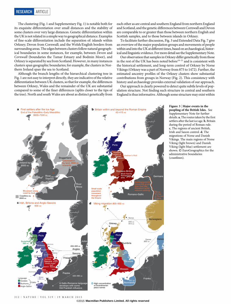
To facilitate further discussion, Fig. 3 and Extended Data Fig. 7 givean overview of the major population groups and movements of peoplewithin and into the UK at different times, based on archaeological, histor-ical and linguistic evidence. For more detail see the Supplementary Note.

Our observation that samples in Orkney differ genetically from thosein the rest of the UK has been noted before18–21 and is consistent withthe historical settlement, and long-term control of Orkney by NorseVikings (Orkney was a part of Norway from 875 to 1472). Further, theestimated ancestry profiles of the Orkney clusters show substantialcontributions from groups in Norway (Fig. 2). This consistency withhistory and archaeology provides external validation of our approach.

Our approach is clearly powered to detect quite subtle levels of pop-ulation structure. Not finding such structure in central and southernEngland is thus informative. Although some structure may exist within

Irish, Britons and Anglo-Saxons 600 AD

Irish

Angles450–500 AD

Saxons

Saxons

Britons

Brit

ons

Bretons

Bernicia

Deira

Lindsey

Elmet

Mercians

Middle Angles

Hwicce

West Saxons

East Angles

EastSaxons

Kent

Dumnonia

Dyfed

Gwynedd

Scots/Irish550 AD

British450 AD

Language Goidelic Brythonic Anglo-Saxon

Celtic

DalriadaPicts

Rheged

Frisians

Franks 420–490 AD

A Gallo-Romance languagedevelops with some Old Frankish influence

Irish

Franks

Normandy911 AD

Norse

840 AD914 AD

Danes865 AD

Norwegians

Danes

Northumbria

Orkney

Danelaw

d Viking migration 800–950 AD

Picts

Scots

Britons

High concentration of Scandinavian place names

Wel

sh

Wessex

Doggerland

Coastline ca. 8000 BC

First settlers after the Ice AgeEnd of the Paleolithic–Early Mesolithic

9600–7500 BC

Ireland by 8000 BC

River Thames

River Rhine

Colonization by land, 9600 BC

onwards

Movement along coast by boat

b Britain within and beyond the Roman Empire 43–410 AD

Irish

Picts

Romano-British

Romano-Gallic

Germans

Hadrian’s Wall

Most heavily Romanized area

Some population movement mostly from Gaul and Rhineland (army veterans settling)

Rhine: frontier of Roman Empire

Greatest extent of Roman control

Jutes

Small-scale population movement throughout the Empire

c

aFigure 3 | Major events in thepeopling of the British Isles. SeeSupplementary Note for furtherdetails. a, The routes taken by the firstsettlers after the last ice age. b, Britainduring the period of Roman rule.c, The regions of ancient British,Irish and Saxon control. d, Themigrations of Norse and DanishVikings. The main regions of NorseViking (light brown) and DanishViking (light blue) settlement areshown. E EuroGeographics for theadministrative boundaries(coastlines).

RESEARCH ARTICLE

3 1 2 | N A T U R E | V O L 5 1 9 | 1 9 M A R C H 2 0 1 5

Macmillan Publishers Limited. All rights reserved©2015

this region, there must have been sufficient movement of people, andhence of their DNA, since the last major invasions of the UK to make itrelatively homogeneous genetically. This does not require large-scalepopulation movements; it could be achieved by relatively local migra-tion over many generations. This region of Britain lacks major geograph-ical and (for the most part since the Roman occupation) geo-politicalbarriers to human movement.

Other UK clusters may well reflect historical events. For example,several genetic clusters in Fig. 1 match the geo-political boundaries inFig. 3c, and may represent remnants of communities/kingdoms pre-sent after the Saxon migrations, while the cluster spanning NorthernIreland and southern Scotland may reflect the ‘Ulster plantations’. TheSupplementary Note contains further observations relating to the gen-etic clustering.

Relative isolation has clearly been a major determinant of fine-scalepopulation structure within the UK. To assess the role of a differentpossible cause, namely differential migration into different parts of theUK, we estimated European ancestry profiles for each of the UK geneticclusters (Fig. 2). Here we must use modern-day groupings, in Europeand the UK, as surrogates for the sources and results of major migra-tion events. Population movements between these events and the pre-sent, involving either the source populations or recipient groups, willattenuate signals of the original migration. For this and other reasons, itis hard to provide definitive explanations for our observations. None-theless, genetic differences persist through many generations and wherewe can check our conclusions against historical evidence, there is goodconcordance. In what follows we focus on the most likely explanationsfor various observations. See Supplementary Note for a fuller discus-sion. For definiteness, we focus on the clustering in Fig. 1 and ExtendedData Fig. 5b, although other levels are informative. Analysis of addi-tional UK and European samples, particularly in regions where ourdata are sparse (for example, central Wales and Scotland, Spain, theNetherlands) would improve our ability to infer historical events.

The observation (Fig. 2 and Supplementary Table 4) that particularEuropean groups (for example, GER3, FRA12, FRA17) contribute sub-stantially to the ancestry profiles of some, but not all, UK clusters stronglysuggests that at least some of the structure we observe in the UK resultsfrom differential input of DNA to different parts of the UK: the absencein particular UK clusters of ancestry from specific European groups isbest explained by the DNA from those European groups never reachingthose UK clusters. A critical observation which follows is that groupswhich contribute significantly to the ancestry profiles of all UK clustersmost probably represent, at least in part, migration events into the UKthat are relatively old, since their DNA had time to spread throughoutthe UK. Conversely, groups that contribute to the ancestry profiles ofonly some UK clusters most probably represent more recent migrationevents, with the resulting DNA not yet spread throughout the UK byinternal migration. ‘Old’ and ‘recent’ here are relative terms—we caninfer the order of some events in this way but not their absolute times.Although we refer to migration events, we cannot distinguish betweenmovements of reasonable numbers of people over a short time or on-going movements of smaller numbers over longer periods.

Applying this approach suggests a relative ordering of the peoplingof the British Isles. For a full discussion, and caveats, see Supplemen-tary Note. Briefly, the earliest migrations whose descendants surviveto make a substantial contribution to the present population are bestcaptured by three groups in our European analyses, GER6 (westernGermany), BEL11 (Belgium), and FRA14 (north-western France). Thesegroups still contribute to current patterns of population differentiation(Fig. 2, see also Extended Data Fig. 6). Other European groups may reflectearly migrations into the UK, but with smaller contribution, includingSFS31 (southern France/Spain), at least part of DEN18 (Denmark), andpossibly parts of Norway and Sweden. A subsequent migration, bestcaptured by FRA17 (France), contributed a substantial amount of ances-try to the UK outside Wales. Although we cannot formally exclude thisbeing part of the Saxon migration, this seems unlikely (see Methods)

and instead it might represent movement of people taking place betweenthe early migrations and those known from historical records. Migra-tions represented by FRA12 essentially only affect Wales and NorthernIreland and/or Scotland. We also see clear signals of some of the knownhistorical migrations and settlements, including the Saxons (GER3,northern Germany, and probably much of DEN18, Denmark) and theNorse Vikings (NOR53–NOR90).

To further shed light on two major migration events, in Orkney andin central and southern England respectively, we applied a distinct ana-lytical tool, GLOBETROTTER22 (Extended Data Figs 8 and 9). Infor-mally, GLOBETROTTER exploits information in the rate of decay ofshared haplotype segments to test for the presence of recent admixture,to identify groups contributing, and then date the admixture.

GLOBETROTTER detected strong evidence (P , 0.01) that thelargest Orkney cluster (Orkney 1) was influenced by a recent admixtureevent with an overall contribution of ,25% of the DNA from groups inNorway, confirming that the Norwegian contribution in the ancestryprofile for this cluster reflects recent admixture (Extended Data Fig. 9).The approach assumed the simplest model (a single pulse of admix-ture), and estimated this to have occurred 29 generations ago (95% con-fidence interval (CI): 18–39 generations), corresponding to year 1100(95% CI: 830–1418), assuming a 28 year generation time22; no clearevidence was found of multiple admixture dates. We expect less preciseestimates for the other two Orkney clusters (due to their smaller samplesize), but these were consistent with those for Orkney 1. For Cent./SEngland the method also detected an admixture event, with a contribu-tion of ,35% of DNA from GER3, the group in north-western Germany,and an estimated date of 38 generations (95% CI: 36–40 generations),corresponding to year 858 (95% CI: 802–914) (Extended Data Fig. 9).The GLOBETROTTER analyses detect likely source populations forthe known historical migrations (Norse Vikings and Saxons, respec-tively) with the estimated proportion contributed by these sources closeto that estimated in the ancestry profiles. Note that a migration event islikely to precede any subsequent population admixture, possibly sub-stantially so, if the migrants mate largely within the migrant group forsome time after their migration. Further, admixture is likely to be agradual process, so that using a model of a single pulse of admixture inGLOBETROTTER is likely to estimate a time after the commence-ment of admixture. For these reasons, the admixture dates estimated byGLOBETROTTER should provide upper bounds on the dates of themigrations22, as for both examples here, where the estimated dates are200 or more years after the known dates of the migrations, suggestingthat the mixing was indeed a gradual process.

After the Saxon migrations, the language, place names, cereal cropsand pottery styles all changed from that of the existing (Romano-British)population to those of the Saxon migrants. There has been ongoinghistorical and archaeological controversy about the extent to which theSaxons replaced the existing Romano-British populations. Earlier geneticanalyses, based on limited samples and specific loci, gave conflictingresults. With genome-wide data we can resolve this debate. Two sepa-rate analyses (ancestry profiles and GLOBETROTTER) show clear evi-dence in modern England of the Saxon migration, but each limits theproportion of Saxon ancestry, clearly excluding the possibility of long-term Saxon replacement. We estimate the proportion of Saxon ances-try in Cent./S England as very likely to be under 50%, and most likely inthe range of 10–40%.

A more general conclusion of our analyses is that while many of thehistorical migration events leave signals in our data, they have had asmaller effect on the genetic composition of UK populations than hassometimes been argued. In particular, we see no clear genetic evidenceof the Danish Viking occupation and control of a large part of England,either in separate UK clusters in that region, or in estimated ancestryprofiles, suggesting a relatively limited input of DNA from the DanishVikings and subsequent mixing with nearby regions, and clear evidencefor only a minority Norse contribution (about 25%) to the currentOrkney population.

ARTICLE RESEARCH

1 9 M A R C H 2 0 1 5 | V O L 5 1 9 | N A T U R E | 3 1 3

Macmillan Publishers Limited. All rights reserved©2015

We saw no evidence of a general ‘Celtic’ population in non-Saxonparts of the UK. Instead there were many distinct genetic clusters inthese regions, some amongst the most different in our study, in thesense of being most separated in the hierarchical clustering tree in Fig. 1.Further, the ancestry profile of Cornwall (perhaps expected to resembleother Celtic clusters) is quite different from that of the Welsh clusters,and much closer to that of Devon, and Cent./S England. However, thedata do suggest that the Welsh clusters represent populations that aremore similar to the early post-Ice-Age settlers of Britain than thosefrom elsewhere in the UK.

In summary, we have presented the first (to our knowledge) fine-scale dissection of subtle levels of genetic differentiation within a coun-try, by using careful sampling, genomic data and powerful statisticalmethods. The resulting genetic clusters, and the characterization of theirancestry in terms of European groups, provide important and novelinsights into the peopling of the British Isles.

Genetic information can augment archaeological, linguistic and his-torical approaches to understanding population history. It also com-plements them, in providing evidence relating to the bulk of ordinarypeople rather than the successful elite. We hope that our study will actas a proof-of-principle for the power of such detailed genetic analyses.

Online Content Methods, along with any additional Extended Data display itemsandSourceData, are available in the online version of the paper; references uniqueto these sections appear only in the online paper.

Received 23 November 2013; accepted 13 January 2015.

1. Cardon, L. R. & Bell, J. I. Association study designs for complex diseases. NatureRev. Genet. 2, 91–99 (2001).

2. Marchini, J., Cardon, L. R., Phillips, M. S. & Donnelly, P. The effects of humanpopulation structure on large genetic association studies. Nature Genet. 36,512–517 (2004).

3. Bodmer, W. & Bonilla, C. Common and rare variants in multifactorial susceptibilityto common diseases. Nature Genet. 40, 695–701 (2008).

4. Cavalli-Sforza, L. L., Menozzi, P. & Piazza, A. The History and Geography of HumanGenes (Princeton Univ. Press, 1994).

5. Quintana-Murci, L. et al. Genetic evidence of an early exit of Homo sapiens sapiensfrom Africa through eastern Africa. Nature Genet. 23, 437–441 (1999).

6. Conrad, D. F. et al. A worldwide survey of haplotype variation and linkagedisequilibrium in the human genome. Nature Genet. 38, 1251–1260 (2006).

7. The 1000 Genomes Project Consortium. An integrated map of genetic variationfrom 1,092 human genomes. Nature 491, 56–65 (2012).

8. Botigue, L. R. et al. Gene flow from North Africa contributes to differential humangenetic diversity in southern Europe. Proc. Natl Acad. Sci. USA 110, 11791–11796(2013).

9. Ralph, P.& Coop, G. The geography of recent genetic ancestry across Europe.PLoSBiol. 11, e1001555 (2013).

10. Hellenthal, G., Auton, A. & Falush, D. Inferring human colonization history using acopying model. PLoS Genet. 4, e1000078 (2008).

11. The Wellcome Trust Case Control Consortium. Genome-wide association study of14,000 cases of seven common diseases and 3,000 shared controls. Nature 447,661–678 (2007).

12. O’Dushlaine, C. T. et al. Population structure and genome-wide patterns ofvariation in Ireland and Britain. Eur. J. Hum. Genet. 18, 1248–1254 (2010).

13. Winney, B. et al. People of the British Isles: preliminary analysis of genotypes andsurnames in a UK-control population. Eur. J. Hum. Genet. 20, 203–210 (2012).

14. The International Multiple Sclerosis Genetics Consortium & The Wellcome TrustCase Control Consortium 2. Genetic risk and a primary role for cell-mediatedimmune mechanisms in multiple sclerosis. Nature 476, 214–219 (2011).

15. Lawson, D. J., Hellenthal,G., Myers, S.&Falush,D. Inference ofpopulation structureusing dense haplotype data. PLoS Genet. 8, e1002453 (2012).

16. Alexander,D.H.,Novembre, J.&Lange,K. Fastmodel-basedestimationofancestryin unrelated individuals. Genome Res. 19, 1655–1664 (2009).

17. Pirinen, M., Donnelly, P. & Spencer, C. C. A. Efficient computation with a linearmixed model on large-scale data sets with applications to genetic studies. Ann.Appl. Stat. 7, 369–390 (2013).

18. Wilson, J. F. et al. Genetic evidence for different male and female roles duringcultural transitions in the British Isles. Proc. Natl Acad. Sci. USA 98, 5078–5083(2001).

19. Capelli, C. et al. A Y chromosome census of the British Isles. Curr. Biol. 13, 979–984(2003).

20. Goodacre, S. et al. Genetic evidence for a family-based Scandinavian settlement ofShetland and Orkney during the Viking periods. Heredity 95, 129–135 (2005).

21. Wells, R. S. et al. The Eurasian heartland: a continental perspective onY-chromosome diversity. Proc. Natl Acad. Sci. USA 98, 10244–10249 (2001).

22. Hellenthal, G. et al. A genetic atlas of human admixture history. Science 343,747–751 (2014).

Supplementary Information is available in the online version of the paper.

Acknowledgements We thank J. Cheshire for his advice. We thank the UK Office forNational Statistics, the National Records of Scotland, and the Northern IrelandStatistics and Research Agency for providing the boundaries used for the UK maps. Wenote that census output is Crown copyright and is reproduced with the permission ofthe Controller of HMSO and the Queen’s Printer for Scotland. We further acknowledgethe provision of maps from Eurostat, which are copyright EuroGeographics for theadministrative boundaries. We acknowledge support from the Wellcome Trust(072974/Z/03/Z, 088262/Z/09/Z, 075491/Z/04/Z, 075491/Z/04/A, 075491/Z/04/B, 090532/Z/09/Z, 084818/Z/08/Z, 095552/Z/11/Z, 085475/Z/08/Z, 098387/Z/12/Z, 098386/Z/12/Z), the Academy of Finland (257654) and the AustralianNational Health and Medical Research Council (APP1053756). P.D. was supported inpart by a Wolfson-Royal Society Merit Award.

Author Contributions W.B. conceived and directed the PoBI project. P.D. directed theanalysis and sample genotyping. B.W., A.B., T.D., K.H., E.C.R. and W.B. collected the UK(PoBI) samples and extractedDNA. IMSGCprovided the European samples’ genotypesand geographical information. Sample genotyping and quality control was performedby WTCCC2 for both the UK and European genotype data. S.L., G.H., S.M. and P.D.performed the major analyses with contributions from B.W., D.D., D.J.L., D.F., C.F., M.R.,M.P. and W.B. M.R. and B.C. provided historical and archaeological information andcontext. G.H. made Extended Data Fig. 2. S.L. produced all the other figures. P.D., S.L.,B.W., G.H., S.M., M.R. and W.B. wrote the manuscript. All authors reviewed themanuscript.

Author Information Genotype data, as well as location information at county level (oraggregated across counties where there are small numbers of samples associated witha particular county), will be made available by the WTCCC access process, via theEuropean Genotype Archive (https://www.ebi.ac.uk/ega/) under accession numbersEGAS00001000672 and EGAD00010000632. Reprints and permissions informationis available at www.nature.com/reprints. The authors declare no competing financialinterests. Readers are welcome to comment on the online version of the paper.Correspondence and requests for materials should be addressed toP.D. ([email protected]).

RESEARCH ARTICLE

3 1 4 | N A T U R E | V O L 5 1 9 | 1 9 M A R C H 2 0 1 5

Macmillan Publishers Limited. All rights reserved©2015

METHODSSamples, genotyping and QC. The sampling scheme and general informationabout the UK sample is described elsewhere13. Briefly, the aim was to collect sam-ples from rural regions of the UK, for whom all four grandparents were born closeto each other. In total 4,371 samples were collected as part of the PoBI project. Ofthese 2,886 were genotyped on the Illumina Human 1.2M-Duo genotyping chipas part of the Wellcome Trust Case Control Consortium 2 (WTCCC2) studies, with2,510 passing the WTCCC2 genotype quality control (QC) procedures23. We thenapplied a geographic filter, which imposed a maximum pairwise distance betweeneach sample’s grandparents’ places of birth of 80 km, leaving 2,039 samples avail-able for analysis. In what follows we refer to these samples as the ‘UK sample(s)’. Wegive a detailed description of the choice of SNPs used for our analyses below.

For the European ancestry profile analysis we used 6,209 samples from theWTCCC2 multiple sclerosis study14, of which 5,682 were cases and 527 were con-trols. We excluded all samples from the UK and Ireland (see ‘treatment of Eire’below). Extended Data Fig. 5a shows a breakdown of sample numbers by region.In the following text we refer to these continental European samples as the ‘Europeansample(s)’. The European samples were genotyped on the Illumina Human 660-Quad chip as previously described14. These samples had already passed throughthe WTCCC2 SNP and sample quality control procedures14.

For all analyses we used intersections of the autosomal SNPs available for theUK and European data sets, constructed in the following manner: we excludedSNPs in the HLA region, and, for analyses involving the European samples, SNPsin major multiple sclerosis associated regions (although any effect of the use ofdisease samples should be small in analyses of genome-wide data). More specif-ically, we first took the full intersection of the UK and European data SNP sets. Weremoved a 15 Mb region surrounding the HLA region on chromosome 6 becausethe European samples were comprised of multiple sclerosis case samples, a diseasewith strong HLA associations. This left 575,236 SNPs that were transferred to thehaplotype inference (phasing) step (see next section). Within the phasing software(IMPUTE2) further SNPs were excluded based on WTCCC2 quality control pro-cedures, which—in addition to IMPUTE2’s internal removal of SNPs due to strandissues or lack of overlap between the SNP array and the reference panel haplotypes—removed 15,211 of these SNPs before phasing. After phasing, SNPs with IMPUTE2info-threshold # 0.975 and SNPs that were singletons among all phased data wereremoved (these data include all POBI and European samples). This left 524,699SNPs. For the analyses using only the UK data (the clustering analysis labelled‘analysis A’ in the next section) 522,862 SNPS were used in the CHROMOPAINTER/fineSTRUCTURE analyses (see next section), as the rest were monomorphic in theUK set of 2,039 individuals. For further analyses, using the European data (labelled‘analysis B’ and ‘analysis C’ in the next section), multiple sclerosis associated SNPs(regions defined by linkage disequilibrium around major loci of suggestive asso-ciation with multiple sclerosis) were removed, as well as some other SNPs for tech-nical reasons. In total this removed SNPs from 56.8 Mb of the genome. This resultedin 515,981 SNPs remaining for the analyses involving European samples. In sum-mary, there were 522,862 SNPs available for the UK clustering analyses, and515,981 SNPs available for the analyses involving European samples. A completelist of rsIDs is available at (http://www.well.ox.ac.uk/POBI).Inference of population structure. To aid in understanding we give an informaldescription of the approach we applied for inferring fine-scale population struc-ture. This is followed by a more detailed elaboration of our analysis. A criticalfeature of the algorithm, unlike other common approaches to detecting popula-tion structure such as principal components, ADMIXTURE16 or STRUCTURE24,is that it explicitly models the correlation structure amongst nearby SNPs due tolinkage disequilibrium, making use of the information in extended multi-markerhaplotypes throughout the genome. This adds substantially to fineSTRUCTURE’spower to detect subtle levels of genetic differentiation. It has been known since theearly HLA studies that methods that account for linkage disequilibrium are moreinformative for studies of human population structure than approaches which treateach locus marginally25.

Very informally, in the fineSTRUCTURE approach, haplotype phase was firstinferred in each sample, after which each resulting haploid genome is broken intopieces, in such a way that for each piece the method identifies the homologouspiece in another individual to which it is most similar. This can be thought of asidentifying the other individual in the collection with the most similar ancestryfor that part of the genome (the average size of these pieces varies across indivi-duals, but has median 0.51 cM with IQR 0.44–0.63 cM). For each individual, onecan tally up the number of pieces over which its genome is closest to each othersampled individual. These individual vectors of similarity counts are then used tocluster together individuals with similar ancestries, using a model-based statisticalalgorithm (fineSTRUCTURE) fitted by Markov chain Monte Carlo. The choice asto the number of clusters, and the assignment of individuals to clusters, is made soas to maximise the posterior probability under the probability model used for

clustering in fineSTRUCTURE. In the PoBI analysis, this yields 53 clusters of indi-viduals. Similar clusters are then merged hierarchically to give a tree which can beused to describe population structure at different levels of granularity, as we describebelow.

More formally, haplotypes were inferred (phased) jointly for all individualsused in the study (that is, the UK and European samples) with IMPUTE226, usingthe default values (see http://mathgen.stats.ox.ac.uk/impute/impute_v2.html#mcmc_options). The reference data used are available from the IMPUTE2 website (http://mathgen.stats.ox.ac.uk/impute/impute_v2.html#reference).

Next, we used the algorithm implemented in the CHROMOPAINTER program15

to represent the DNA of individuals as mosaics of the DNA from other individuals.We performed three separate CHROMOPAINTER analyses:

A. Form each haplotype of a UK individual as a mosaic of all UK haplotypes exclud-ing those of that individual.B. Form each UK haplotype as a mosaic of all European haplotypes.C. Form each haplotype of a European individual as a mosaic of all European hap-lotypes excluding those of that individual.

For each analysis, A–C, we ran the algorithm implemented in CHROMOPAINTERas recommended by the authors, except for a minor change to the value of a singleparameter for analysis A, implemented for technical reasons. Specifically, weinitially applied CHROMOPAINTER to a subset of individuals and chromosomes(chosen as described below) using 10 iterations of its expectation-maximization(EM) algorithm to infer the genome-wide average switch and global emissionrates in CHROMOPAINTER’s Hidden Markov model. We averaged the inferredvalues of each across the chromosomes and individuals used, weighting chromo-somes by their relative size, and fixed these final switch and global emission ratesin a final run of CHROMOPAINTER on all individuals and chromosomes. Thisfinal CHROMOPAINTER run gave the final ‘counts’ and ‘lengths’ values used inall subsequent analyses. For analysis A, we inferred switch and global emissionrates averaging across chromosomes 4, 10, 15, 22 (using weights of 187, 131, 81 and34, respectively) and 20 individuals from each of 30 UK sample regions (countiesor districts from which the PoBI samples were collected, from across the whole UK),starting with an initial switch rate of 400,000/(2NUK), where NUK is the number ofsamples used for the UK analyses, and a default emission rate. For analyses B and C,we inferred switch and global emission rates averaging across chromosomes 1, 8,15, 22 (using weights of 219, 142, 81 and 34, respectively) for 20 individuals from eachof 30 United Kingdom regions, and 20 individuals out of every 200 in a combinedfile of all European subjects, starting with an initial switch rate of 400,000/(2NE),where NE is the number of samples used for the European analyses, and a defaultemission rate. Previous work with CHROMOPAINTER has shown that deviations ofthe switch rate (even up to a factor of 10) have little effect on CHROMOPAINTER’sinference (data not shown). Finally, for analysis C, we set the expected number ofhaplotypic segments to define a region (that is, the ‘-k’ switch) to CHROMOPAINTER’s default value of 100 in order to estimate a normalization parameter (denotedby ‘c’) subsequently used by the clustering program fineSTRUCTURE15. In con-trast, we set this value to 50 (that is, using ‘-k 50’) for analysis A. This slightdeviation from CHROMOPAINTER’s default value was implemented for analysisA because some UK individuals shared relatively long haplotype segments withother UK haplotypes, such that they did not always have 100 total such segmentsacross the entirety of some of the smaller chromosomes. We used the June 2008build 36 genetic map from the HapMap webpage (http://hapmap.ncbi.nlm.nih.gov/downloads/recombination/2008-03_rel22_B36/rates/).

CHROMOPAINTER provides estimates of the counts of haplotype segments andtotal length of DNA (in cM) for which an individual shares most recent commonancestry with a set of other individuals. When summed across all 22 autosomes werefer to the vector of these counts as the ‘copying profile’ for that individual. Forexample, in analysis B, CHROMOPAINTER gives the counts of haplotype seg-ments and total length of DNA for which each UK individual shares most recentcommon ancestry with each European individual. These values are given for chro-mosome 1–22 of each UK individual, and are also summed to give a genome-widetotal across the autosomes (in the case of the counts data, the copying profile).Furthermore, within a UK individual, these values can be summed across any group-ing of European individuals (for example those sampled from the same geographicregion or assigned to the same European group, see below) providing an estimateof the counts of haplotype segments and/or total length of DNA for which each UKindividual shares most recent common ancestry with any European group (a groupcopying profile). It is natural to average these values across UK individuals assignedto the same cluster (see below) to get average values for all UK individuals from aparticular cluster; a ‘copying vector’ for the cluster as a whole.

For analyses A and C, described above, we used the algorithm implementedin the program fineSTRUCTURE15 to group the UK and European individualsrespectively into genetically relatively homogeneous clusters. The fineSTRUCTUREprogram takes as its input the counts of haplotype segments for which each individual

ARTICLE RESEARCH

Macmillan Publishers Limited. All rights reserved©2015

shares recent common ancestry with every other as inferred by CHROMOPAINTER(summed across all chromosomes, the copying profile). The choice to use countsin this analysis is motivated by the underlying ‘painting’ model used by CHROMOPAINTER, in which segments are shared with individuals chosen independentlyfrom one another, and there is a constant switch rate between segments. Underthis model, each segment provides an equal amount of independent information,while segment lengths are uninformative, so the segment counts provide a naturalbasis for inference, and this is why they are used. However, we note that in practicefineSTRUCTURE attempts to allow for departures from this modelling assump-tion (which is expected to only be an approximation) through a scaling parameteron the (log-) likelihood. Moreover we believe there is often useful informationprovided in, for example, the fact that segments shared between genuinely closelyrelated groups tend to be longer on average, akin to the idea of long segments shared‘identical by descent’ with respect to some founder population. Exploring and usingthis length information may provide an interesting topic for future work.

We initially put all of our individuals into a single cluster at iteration 0, but other-wise used default values when running fineSTRUCTURE (see ref. 15 for details).Each Markov Chain Monte Carlo (MCMC) iteration of fineSTRUCTURE providesthe number of clusters and the cluster membership of each individual, sampledaccording to their posterior probabilities under the fineSTRUCTURE model. Wesampled values every 10,000 iterations for 1 million MCMC iterations followingeither 1 million (analysis A) or 3 million (analysis C) ‘burn-in’ iterations. Startingfrom the MCMC sample with the highest posterior probability among all samples,fineSTRUCTURE performed 100,000 additional hill-climbing moves to reach itsfinal inferred state.

Next we undertook an additional step to improve fineSTRUCTURE’s inferencefor cluster membership. This is an addition to the fineSTRUCTURE algorithm15.While fineSTRUCTURE’s final inferred state has been shown to give reasonableresults in practice15, it relies heavily on a single MCMC sample observation. Althoughthis single sample is the one with maximum posterior probability among all MCMCsamples, the probability has been calculated assuming fixed (sampled) values for alarge number of parameters that include the total number of clusters, each individual’sfinal inferred cluster assignment, and other modelling parameters. Therefore, a con-cern is that the posterior distribution will be relatively flat across such an extensivestate space, such that fairly divergent parameter values may result in similar pos-terior probabilities. In contrast, the marginal posterior distribution of each indi-vidual’s cluster assignment across all MCMC runs should be substantially moreinformative, improving the assignment of individuals to clusters. Informally, bychance alone any given individual may not be in its own optimal (highest proba-bility) cluster in the final inferred state, despite the overall posterior probabilitybeing at its maximum. We thus seek to reassign any such individuals to their mostprobable cluster. We therefore leverage the marginal information of each indivi-dual’s cluster assignment from the values of the MCMC samples recorded every10,000 iterations (see above) in order to re-assign individuals to clusters. Specifi-cally, assuming we have N total individuals and M MCMC samples, and startingfrom the K clusters in fineSTRUCTURE’s ‘final inferred state’, we performed thefollowing procedure:1. We find the number xi

(m) of individuals that cluster with individual i (includingindividual i itself) in MCMC sample m, for i 5 1,...,N and m 5 1,...,M.2. We furthermore find the number yik

(m) # xi(m) of individuals that both cluster

with individual i in MCMC sample m and that are in cluster k of the final inferredstate, for k 5 1,...,K.3. We re-assign each individual i to the cluster k with the maximum value ofP

m 5 1,...M [yik(m) / xi

(m)] across all k in 1,...,K. These re-assignments give a new finalinferred state; note these re-assignments can reduce the total number of clusters K.4. We repeat steps 1–3 for 50 iterations.This procedure gives the final cluster assignments for each individual.

One feature of this additional procedure used for reassigning individuals toclusters is that we obtain measurements of the confidence in the assignment ofeach individual i to each cluster k. For each individual i, the values of

Pm 5 1,...M

[yik(m) / xi

(m)] from the final iteration can be normalized across k to sum to one,and stored in the K-vector PK,i. These quantities have a natural interpretation as ameasure of the confidence associated with the assignment of individual i to eachcluster k. Note that we assign individual i to the cluster k for which the value of themeasurement is maximal. Call this maximal value Pk_max,i. It is possible to apply athreshold t, 0 ,t , 1, to the assignment of individuals to clusters so that an indi-vidual is only assigned to a cluster if Pk_max,I . t. If not, then the individual may beremoved from subsequent analyses. We investigated the effect of setting such athreshold t. The main observation is that applying a threshold has very little effecton the make-up and distribution of clusters across the UK, nor on downstreamanalyses (data not shown). For further discussion see Supplementary Note.

One possible consequence of this extra procedure is to reduce the final numberof clusters inferred from that of the so-called final inferred state. For analysis A,

the final number of UK clusters inferred, after the extra procedure, is 53 (the initialfinal inferred state had 55). For analysis C the final number of European groupsinferred is 145 (no change to the initial final inferred state).

We assessed convergence of the fineSTRUCTURE MCMC runs in variousways. This included running independent chains, and comparing aspects of theassignments of individuals to clusters, and the results of downstream analyses,between the two chains. Reassuringly, given the size of the state space being ex-plored, these diagnostics confirmed mixing of the MCMC chains (Extended DataFig. 2).

Using the final assignments, we used fineSTRUCTURE to construct a ‘tree’ inthe default manner described in ref. 15 by successively merging pairs of clusters.Starting at the final cluster assignments, fineSTRUCTURE merged the pair of clus-ters whose merging gave the smallest decrease to the posterior probability amongall possible pairwise merges. This gives the next level up in the tree (with one fewercluster). We repeat this merging process at the new level and continue until just twoclusters remain. Figure 1 shows the assignment of individuals to clusters for thelevel of the tree when 17 clusters remain. The final cluster assignments and theassignments of individuals to clusters at all levels of the tree are provided in Sup-plementary Figs 1.1–1.24 for the UK clustering analyses (A). The tree so obtained isa hierarchical clustering tree and should not be interpreted as a phylogeny. None-theless there is information about the strength of the differentiation between clus-ters in these trees.

It is possible to use the vectors of measures PK,i defined above, of the confidenceassociated with the assignment of individual i to each cluster k in the final inferredstate, to reassign individuals to clusters at any level of the tree. Consider the fol-lowing. Define the lowest or finest level of the tree, the level relating to the finalcluster assignments, to be LK, where K is the number of clusters in the final inferredstate. Then define each level of the tree to be LJ, where J in (2, 3, …, K) is the numberof clusters at the level of interest. For a given level of the tree LJ, each cluster CJ,j, j in(1, …, J), is made up of one or more clusters at the lowest level of the tree, mergedinto a single cluster. For example, the large UK cluster in central and southernEngland at the level containing 17 clusters (depicted in Fig. 1, red squares) is theunion of eleven smaller clusters from the final inferred state. For each individual iit is possible to define a new J-vector of measures PJ,i, for level LJ, where for eachcluster CJ,j we sum the values in PK,i for all clusters that are merged to form CJ,j, andstore the result in component j of PJ,i. Thus, for our previous example of the largecluster in central and southern England at the level containing 17 clusters, for eachindividual i we sum the values relating to the eleven constituent clusters at the finalinferred state that make up this larger cluster, and use this as the measure of con-fidence that the individual i is assigned to the larger cluster. We can use the vectorof measures PJ,i so-defined to reassign individuals to the cluster for which PJ,i ismaximal. This will potentially result in some individuals being reassigned to a dif-ferent cluster from the one to which they were assigned by the standard tree build-ing method. For example, we see this has occurred for exactly one individual inExtended Data Fig. 1, resulting in the different total numbers assigned to the redsquare and purple cross clusters in Extended Data Fig. 1 when compared to Sup-plementary Information Fig. 1.16 (both depicting 17 clusters). One advantage of thisprocess is that we can interpret PJ,i as a measure of the confidence of the assignmentof an individual i to each cluster at the given level LJ. We can also set a threshold tand examine which individuals have lower confidence assignments to their cluster,where by ‘lower confidence’ we mean that the maximum value in the vector PJ,i isless than t. We depict this for the UK clustering at the level of 17 clusters in Ex-tended Data Fig. 1, when we set t 5 0.7.Other methods for detecting population structure. We implemented principalcomponents analysis (PCA) using the package MMM17. We applied PCA to theintersection of the SNPs used for PCA in the WTCCC2 project23 and the SNPspassing quality control filters in UK sample in this paper. This resulted in 188,329SNPs with minor allele frequency .0.05 in the UK population. These SNPs aredistributed approximately evenly with respect to the genetic distance across the 22autosomes. We excluded all SNPs in regions with unusually high loadings basedon visual inspection of the first 20 axes of PCA applied to the UK control samplesof WTCCC2. The results are shown in Extended Data Fig. 3a.

We also applied the program ADMIXTURE16 to these same data, using defaultsettings as recommended by the authors. The ADMIXTURE model effectively as-sumes independence of the markers used across the genome. We ran ADMIXTUREthree times, corresponding to three different choices for the number of clusters tobe used for classification (K). To understand the method in the simplest cases weset K 5 2 and K 5 3, and for comparison to the results presented in our main ana-lyses we set K 5 17. The results are shown in Extended Data Fig. 3b.Continuous or discrete frameworks for modelling and inferring populationstructure. There is a general issue when modelling genetic variation from spa-tially structured populations as to whether to use models which characterize thepopulation as comprised of distinct subpopulations, or at the other extreme to model

RESEARCH ARTICLE

Macmillan Publishers Limited. All rights reserved©2015

the population in continuous space, without distinct subgroups, where isolation bydistance is the primary factor in giving rise to geographical substructure16,24,27,28.Both are obviously oversimplifications for natural populations, and in particularfor humans, and are more naturally thought of as caricatures and as endpoints of aspectrum, with debate as to which might be closer to capturing the important fea-tures of historical human demography.

One potential criticism of the fineSTRUCTURE approach is that it is embed-ded in a framework of discrete subgroups. There is an obvious sense in whichfineSTRUCTURE is closer to this framework: it explicitly estimates a set of sub-groups in the population, on the basis of patterns of shared ancestry. Althoughthis is a description of the population, rather than a model of it, it might well bemore natural or useful if there is, in reality, some underlying discreteness. On theother hand, the hierarchical tree estimated by fineSTRUCTURE allows viewing ofthe population at multiple levels of clustering. This does not stipulate a fixed num-ber of subgroups, and instead provides a complex description of the underlyingstructure—in effect zooming in from the coarsest partition of the population astwo subgroups to examine finer and finer partitions. Taken together, we arguethat this approach is better suited to capturing the complexities of real popula-tions than had it only described a single set of discrete subgroups. Our approach,of probabilistically classifying individuals into groups at a particular level, ratherthan forcing them to belong to exactly one cluster, also allows some flexibility in aworld where there is smoother variation with geography.

Clearly some, but not all, aspects of human demography will be influenced bythe dynamics of isolation by distance. Conversely, cultural, linguistic, and geograph-ical barriers will all tend to encourage boundaries, and hence discreteness of sub-groups. We are encouraged by the fact that the multi-level descriptive frameworkof fineSTRUCTURE, as applied to the subtle levels of population structure withinthe UK, is clearly capturing real effects, as evidenced for example by the concordancewith geography, largely non-overlapping clusters (compared with ADMIXTURE),confident assignment of individuals to clusters in most cases (typically except whereclusters overlap geographically), and its ability to detect groups which reflect knownhistorical events.Estimating ancestry profiles. To understand the genetic make-up of different ge-netic clusters in the UK with respect to potential ancestral populations we performedthe following analyses. For analysis B (above) the CHROMOPAINTER algorithmprovides estimates of the proportion of each UK individual’s DNA that is most closelyrelated ancestrally to each European individual, among all the sample members.These proportions can then be summed across groups. These proportions approx-imate the fraction of an individual’s DNA that coalesces, back in time, most re-cently with each particular sampled individual15. Because in humans these coales-cence events can be far back in time relative to population separation times, weexpect them to often predate population splits (that is, we expect incomplete lin-eage sorting). This leads to differences in the amount of DNA copied from differ-ent European groups being subtle, in a sense adding noise. The amount of noisedepends on the number of individuals sampled—and thus potentially sharing DNA—in the different groups, with larger sample sizes likely to reduce noise. In addition,we rely on informative variation patterns to identify individuals from whom DNA iscopied, adding additional noise, which may systematically vary across the genome.To account for this noise we follow ref. 22, so that at each level of the hierarchicalclustering tree of the UK samples, and for a fixed level (see main text) of the Euro-pean samples’ hierarchical clustering tree, we perform multiple linear regressionas follows. For each level of the hierarchical clustering tree of the UK samples, andfor the set of G (5 51) groups inferred for Europe we perform the following linearregression. Let YP be a G-vector describing the average proportion of DNA genome-wide that a cluster P of UK individuals copies from each of G groups of Europeanindividuals, as inferred by CHROMOPAINTER. That is, element g of YP consistsof CHROMOPAINTER’s total genome-wide length (in cM) of all haplotype seg-ments inferred to be most closely related ancestrally to any individual of Europeangroup g, normalized to sum to unity across all g in 1,...,G within a UK individualand then averaged across all individuals in the UK cluster P. We use copying lengths,rather than counts (used in the clustering itself), for this analysis because all indivi-duals have the same total genetic length, but this length may be broken into differingnumbers of copying segments in different individuals. Thus it is straightforward tointerpret coefficients in the below linear regression, in terms of the fraction of the ge-nome contributed by different components in the mixture, using copying lengths,but interpretation would be more difficult using counts of shared DNA segments.Analogously, let Xg be a G-vector describing the average proportion of DNA that theEuropean individuals of group g copy from each of the G European groups as inferredby CHROMOPAINTER, including their own group (though note individuals are notallowed to copy from their own haplotypes in CHROMOPAINTER). We assume

YP~b1X1zb2X2z . . . zbGXG, ð1Þ

and solve simultaneously for the bg under the restriction that each bg $ 0 andPG

g~1bg~1, using a slight adaptation of the non-negative-least-squares (nnls) func-

tion in the statistical software package R (see ref. 29).We interpret the inferred value for bg as the average proportion of genome-

wide DNA of a UK individual from cluster P that is most closely related ancestrallyto European group g. We refer to these vectors as ‘ancestry profiles’.

To assess statistical uncertainty in our estimates of the bg for each UK cluster P,we perform a bootstrap procedure where we re-sample the chromosomes of theNP UK individuals in this group (constructing pseudo-individuals by samplingpairs of chromosomes for each of the autosomes). In particular, for each boot-strap iteration, we randomly sample the G-vector of CHROMOPAINTER outputacross these UK individuals NP times with replacement for each chromosome1–22. We then generate each of NP ‘pseudo-individuals’ by randomly summing22 pairs of these samples (without replacement), one pair per chromosome, andthen summing across the first, respectively the second, member of each pair beforerescaling the resulting G-vectors to sum to unity. Averaging each element of theG-vectors across these NP pseudo-individuals gives us a new re-sampled value ofYP, which we then substitute into (1) above to generate new inferred values of thebg. We repeat this procedure 1,000 times, reporting the inner 95% quantiles of thesampling distribution for a given European group g across these 1,000 bootstrapre-samples (see Supplementary Table 4 and Extended Data Fig. 6a).Assessing the strength and robustness of the inferred population structure—FST, identity by descent (IBD) and total variation distance (TVD). Using the sameset of SNPs that were used for the PCA analyses (see above) we analysed pairwiseFST both between the sample collection districts, and between the 17 inferred clustersfrom our main analysis using the method implemented in the program Eigensoft30.The complete matrices of pairwise FST values are given in Supplementary Tables 1and 2.

To investigate the effect that recent shared ancestry may have on our analyseswe calculated a measure of pairwise IBD and compared its distribution withinclusters to its distribution across the whole sample. This measure uses a hiddenMarkov model (HMM) to estimate IBD across the genome14. The measure is likelyto be useful when the shared relatedness is just a few generations in the past, allow-ing the identification of pairs of individuals in our UK sample that are reasonablyclosely related. The results are plotted in Extended Data Fig. 4. Reassuringly, theseconfirm that levels of relatedness within clusters are typically similar to those betweenclusters, and hence that our observed clusters are not an artefact of a sampling schemewhich preferentially selected closely related individuals from regional localities.

To quantify the strength of differences between the inferred clusters we performthe following analyses. As noted above we can summarize the copying profiles of allthe samples in a given cluster X to produce a characteristic ‘copying vector’ x 5 (x1,x2,…,xn); the average (across individuals in cluster X) proportion of each indi-vidual in cluster X’s closest ancestry that is attributed to individuals from each ofthe clusters, Y 5 (Y1, Y2,…,Yn), where n is the number of inferred clusters. In fact,this copying vector can be calculated for any group of samples (that is, not onlythe inferred clusters). One can use these vectors to test if the clusters inferred byfineSTRUCTURE are capturing significant differences in ancestry, and to give asense of the strength of the differences observed. Given a pair of inferred clusters (Aand B) and their copying vectors (a and b respectively) one can calculate the totalvariation distance (TVDCV) between the pair:

TVDCV A,Bð Þ~0:5|Pn

i~1ai{bij jð Þ:

TVDCV can be interpreted as a measure of the difference between the two clusters.(As the copying vectors are discrete probability distributions over the set of clus-ters, total variation distance is a natural metric for quantifying the differencebetween them.)

Furthermore, given a pair of clusters (A and B) one can randomly reassign theindividuals in the clusters, maintaining the cluster sizes, to obtain a new pair ofclusters (A’ and B’, of the same size as A and B, respectively). One can then cal-culate the copying vectors (a’ and b’) for the new clusters A’ and B’, and the totalvariation distance between them. Repeating this process m times one can obtain aP value from a permutation test of the null hypothesis that, given the cluster sizes,the individuals in the two clusters are assigned randomly to each cluster. Here theP value is the proportion of the m permutations where TVDCV A0,B0ð Þ§TVDCV A,Bð Þ.Supplementary Table 3 shows the value of the TVDCV statistic for all pairs of the17 clusters used in our main analyses.

Similarly, rather than using the copying vectors for a pair of clusters (A and B),one can use the ancestry profiles of the clusters (a and b) to calculate the total var-iation distance between the ancestry profiles of a pair of clusters (TVDAP):

ARTICLE RESEARCH

Macmillan Publishers Limited. All rights reserved©2015

TVDAP A,Bð Þ~0:5|Pn

i~1ai{bij jð Þ

TVDAP can be interpreted as a measure of the difference between the ancestryprofiles of the two clusters. (Again, as ancestry profiles are discrete probabilitydistributions, total variation distance is a natural metric for quantifying the dif-ference between them.)

As above, one can permute the individuals that are assigned to each cluster,maintaining the cluster sizes, and calculate the ancestry profiles of the resultingclusters (A9 and B9) and the total variation distance between them. As before, repeat-ing this process m-times one can obtain a P value from a permutation test of thenull hypothesis that, given the cluster sizes, the individuals in the two clusters areassigned randomly to each cluster with respect to their ancestry profile. Here theP value is the proportion of the m permutations where TVDAP A0,B0ð Þ§TVDAP A,Bð Þ.Supplementary Table 5 gives TVDAP for all pairs of ancestry profiles for the 17 UKclusters used in our main analyses, and gives the associated P values based on 1,000permutations.Assessing the accuracy and robustness of the ancestry profiles. We undertook anumber of simulation studies, generating data with similar properties to the actualdata, to assess the accuracy of the estimated ancestry profiles. These suggested goodaccuracy of the major components of our estimated ancestry profiles.

A major challenge for this kind of simulation study is in simulating data whichhas similar properties to the real data. The subtle similarities and differences withinand between our various UK clusters and European groups are generated by theircomplicated shared and distinct demographic histories. This true demographichistory is unknown and might not be well approximated by simple models that canbe simulated from, and so it is not possible to simulate realistic data from the appro-priate model31. Instead, we used subsamples of the real data for our simulationstudies. This has the advantage that it replicates patterns in the real data, but thedisadvantage that simulation studies must be based on smaller sample sizes thanthe actual study. (Since some of the data are needed to simulate the scenario ofinterest, and the rest of the data to analyse that scenario, so neither the simulateddata set, nor the data used for analysis, can be as large as the actual data set.)

For each simulation scenario described below, we generated N simulated indi-viduals as mixtures of two populations A and B intermixing l generations ago inproportions a, b (5 1 2 a) respectively, closely following established approaches22,32,33.Informally, to simulate an admixed haploid chromosome we did the following: agenetic distance x (in centimorgans) was sampled from an exponential distributionwith rate l/100. The first x cM of the simulated chromosome was composed of thefirst x cM of a real data chromosome selected randomly from either population Aor B according to the proportions of admixture a and b (the specific values used aregiven below). Then a new genetic distance was sampled from the same exponentialdistribution (rate 5 l/100), and the process repeated until an entire simulatedchromosome was generated. This was repeated for all 22 autosomes, resultingin a single (haploid) set of chromosomes for one individual. We did this 2N times,generating 2N full sets of haploid autosomes. (To limit the chance of multiple sim-ulated individuals copying from the same real data individual at any location in thegenome, wherever possible the new piece of chromosome sampled was selectedfrom the pool of chromosomes in the selected population (A or B) for which noother previously simulated chromosome had copied at the same location. Whenthis was not possible, a chromosome was selected at random from the selected pop-ulation (A or B), see ref. 22. Diploid individuals were constructed by aggregatingtwo full sets of haploid chromosomes, making N simulated individuals in total.

We considered three scenarios of two populations admixing, and for each ofthese scenarios we considered three proportions of admixture for the second group(b 5 0.1, 0.25 and 0.5). This yielded the following nine sets of simulations:(1) ‘Italy and northern Germany’: N 5 25, l 5 40, b 5 0.1, 0.25 and 0.5, derivedby mixing 30 randomly sampled individuals from the Italian Group ITA36 (whichcontains 284 individuals) with 10 randomly sampled individuals from GER3 (58individuals).(2) ‘North Wales and Norway’: N 5 40, l 5 29, b 5 0.1, 0.25 and 0.5, derived bymixing 75 individuals from the N Wales cluster with 10 randomly sampled indi-viduals from NOR72 (116 individuals) and 10 from NOR71 (148 individuals).(3) ‘North Wales and Denmark’: N 5 25, l 5 40, b 5 0.1, 0.25 and 0.5, derived bymixing 75 individuals from the N Wales cluster with 20 randomly sampled indi-viduals from DEN18 (319 individuals).

These simulations were chosen both to test our model’s ability to infer sourcesof admixture and their proportions from distinct European groups (simulation 1);as well as to mimic admixture events we infer in our main analyses, that is, relatingto the Norwegian Viking (simulation 2) and Anglo-Saxon (simulation 3) migra-tions into the UK. Simulations (2) and (3) use samples from the N Wales cluster,which we infer has little evidence of DNA influx from the Norwegian Vikings andAnglo-Saxons, and mixes them with groups containing primarily individuals sampled

from Norway (2) or from Denmark (3). These simulations are used to modeladmixture between the ‘ancient’ British population (that is, genetically constitutedas it was before the Saxon invasion) and Norwegian Viking or Anglo-Saxon settlers,respectively. Simulation (2) further assesses our model’s ability to distinguish twodistinct Norwegian sources of admixture from among 12 different groups prim-arily containing samples from Norway.

For each simulated data set we estimated ancestry profiles as follows. We usedCHROMOPAINTER (see above) to represent each of the 2N simulated haplotypesas a mosaic of all the European haplotypes except those used for the relevantsimulations. Specifically, the 40 samples from ITA36 and GER3 used for the sim-ulations in the ‘Italy and Northern Germany’ scenario (1) were removed from theCHROMOPAINTER analysis for scenario (1). Similarly the European samplesused for the simulations in (2) and (3) were removed in their respective CHROMOPAINTER analyses. This ensures that the actual admixing individuals are notsampled when forming the mosaics. We used the estimated switch and emission ratesfrom the main analysis, described in ‘Inference of population structure’ above.

Recall the ancestry profiles are determined by fitting a linear mixture modelthat utilizes both the CHROMOPAINTER copying profiles derived from makingup the ‘target group’ (here the simulated samples, in our main analysis the UKsamples within a cluster) haplotypes from the ‘source groups’ (here the Europeansamples except those used in the simulations, in our main analysis all the Euro-pean samples) haplotypes, as well as the CHROMOPAINTER copying profilesused for the clustering of the ‘source groups’. To obtain the latter we adapted theresults from the existing CHROMOPAINTER analysis C (see ‘Inference of popu-lation structure’ above) as follows. (It would be computationally prohibitive torerun the full CHROMOPAINTER analysis for each of the nine simulated datasets.) For each European individual’s copying profile the elements associated withthe European samples used in the simulations were removed. Then, for each ofthe 51 European groups, we averaged these adjusted copying profiles across allindividuals assigned to the given group (excluding any individuals used in the rele-vant simulations) as described in ‘Inference of population structure’, and used theadjusted copying profiles for the 51 EU groups as covariates in our linear mixturemodel as described in estimating ancestry profiles.

This post-hoc adjustment of the copying profiles for each of the 51 Europeangroups assumes that if we had repeated the CHROMOPAINTER analysis for therelevant reduced set of European samples, the copying profile of the parts of thechromosomes previously associated with the removed samples is redistributedevenly across all the other European individuals. This is inherently conservativeas it is more likely that by excluding, for example, 10 of the 58 GER3 samples fromthe ‘new’ GER3 group would have resulted in an increase of copying from theother 48 GER3 samples, relative to the increase in copying from individuals fromother European groups. Thus the performance of our approach for determiningancestry profiles in our simulation study is likely to be an under-representation ofthe performance of our approach in the main data analyses.

Furthermore, we only used a relatively small number of individuals from eachof ITA36, GER3, NOR71, NOR72 and DEN18 in the simulations, to ensure a suf-ficient number of remaining individuals from each to use for inferring the ances-try profiles. As a consequence, the number of simulated individuals we generatedis rather small, consisting of only 25 or 40 individuals per simulation, comparedto our main analysis (using the real data) where many of the clusters were signifi-cantly larger. We expect the increased sample size for the majority of clusters usedin our main analyses to improve our inference of ancestry profiles relative to thesimulations, substantially so in some cases such as Cent./S England which contains1,044 individuals.

We also adopted an alternative simulation approach for the scenarios repre-sented by (1)–(3) above using a forwards-in-time simulation method, initialisedfrom real data, as previously described22. In each case, we combined a subset of thesame randomly sampled individuals from populations A and B above (for example,for (1), the 30 individuals from ITA36 and the 10 individuals from GER3) into asingle pool population, which we then simulated forwards in time for the same lgenerations as used above. To imitate the three simulations for scenario (1) abovethis pool population contained respectively (20, 60, 60) haplotypes from ITA36and (20, 20, 7) haplotypes from GER3 to approximate admixture contributions of(0.5, 0.25, 0.1) from GER3. Similarly for scenario (2) the pool population contained(40, 120, 150) haplotypes from N Wales and (40, 40, 18) haplotypes from NOR72/NOR71 (half from each); and for scenario (3) (50, 150, 150) haplotypes from NWales and (50, 50, 18) haplotypes from DEN18.

To create the next generation of haplotypes following this admixture event, werandomly sampled two distinct parental haplotypes (each comprising a full set of22 single chromosomes from one individual) from the pool. We composed a newset of haplotypes for an individual in the next generation as a mosaic of chunks fromthese two parent sets, with switches in the mosaic based on the HapMap Phase 2genetic map (June 2008, build 36 genetic map, as above). More specifically, we

RESEARCH ARTICLE

Macmillan Publishers Limited. All rights reserved©2015

determined the number of recombination breakpoints on each chromosome bysumming a random sample from a Bernoulli distribution with probability 0.5 (whichmodels the expected obligate crossover per generation per chromosome) and arandom sample from a Poisson distribution with rate equal to the total genetic lengthof the chromosome in Morgans minus 0.5 (which models the remaining crossovers).We then sampled the physical location of each of the breakpoints independentlyaccording to their relative genetic map value, copying segments on either side of abreakpoint without mutation from the chromosome’s two different parents. In thefirst generation after the admixture, we repeated this process to generate 500 full(that is, chromosomes 1–22) sets of haplotypes. For the remaining l{1 genera-tions, 500 new full sets of haplotypes were each simulated in the same manner as amosaic of chunks from two distinct full sets of haplotypes randomly sampled withreplacement from the previous generation. After l generations, we randomly sam-pled distinct haplotypes (that is, without replacement) to form N individuals forsubsequent analysis, where N is the same as in the relevant scenario of (1)–(3) above.We then inferred ancestry proportions in these N simulated individuals in thesame manner described above.

The resulting ancestry profiles from all 18 simulation studies (2 simulation methodstimes 3 scenarios times 3 admixture proportions (b)) are given in SupplementaryTable 6.Dating admixture events in Orkney and southeast England. We ran GLOBE-TROTTER22 to estimate the time of the major admixture events contributing to themake up of the Cent./S England cluster and the three clusters in Orkney (Westray,Orkney 1 and Orkney 2) using the 51 European groups as surrogates for the puta-tive admixing ‘source groups’ (that is, using analysis B from ‘Inference of popula-tion structure’ above) and assuming a single ‘pulse’ of admixture when analysingeach UK cluster. We closely follow the application of GLOBETROTTER as describedby the authors. In short, CHROMOPAINTER identifies the segments of DNA withineach UK individual’s genome that are most closely related ancestrally to each Euro-pean group, as described in ‘Inference of population structure’. GLOBETROTTERmeasures the decay of association versus genetic distance between the segmentscopied from a given pair of European groups. Assuming a single pulse of admixturebetween two or more distinct admixing source groups, theoretical considerationspredict that this decay will be exponentially distributed with rate equal to the time(in generations ago) that this admixture occurred34. GLOBETROTTER jointly fitsan exponential distribution to the decay curves for all pairwise combinations ofEuropean groups and determines the single best fitting rate, hence determiningthe most likely single admixture event and estimating the date it occurred. Insteadof requiring specific genetic surrogates to represent each admixing source groupinvolved in the admixture, as in other dating approaches such as ROLLOFF35,GLOBETROTTER aims to infer the haplotype composition of each source groupfor the admixture as a linear combination of those carried by sampled groups (thatis, a linear combination of the 51 European groups). This results in the admixedgroup themselves automatically being represented in the same form—as a mixtureof mixtures—consistent with the linear estimation procedure we applied for eachUK group, before estimating admixture dates for each group.

The following provides more details on our approach for dating and estimatingadmixture proportions within a single UK cluster; full details of the GLOBETROTTERmethod are provided in ref. 22. For each haploid set of chromosomes of each indi-vidual from a given UK cluster, we consider the genome-wide mosaic inferred byCHROMOPAINTER in the UK on Europe analysis (analysis B from ‘Inference ofpopulation structure’ above). In this manner each UK sample’s haploid genome ispieced together as a series of ‘chunks’, with each chunk a contiguous segment ofDNA best matching a European sample inferred to be most closely related ances-trally to that segment. We note that CHROMOPAINTER infers these mosaics foreach individual many times in a probabilistic manner, so we can sample from theset of mosaics for a given individual. We sampled 10 such mosaics for each haploidgenome of each UK individual in the cluster we are focusing on, giving 20 totalmosaics for each UK individual.

Consider two of these 20 mosaics (these two could be the same sampled mosaic).We compare each chunk on mosaic 1 to each chunk on mosaic 2. For each pair ofchunks, we record the two European groups (perhaps the same) copied at each chunk(or more precisely, the group of the European individual inferred to be closest tothe UK individual’s chunk) in the pair and the genetic distance between the twochunks’ midpoints. We remove any chunk pairs where this genetic distance is lessthan 1 cM (to avoid the effects of within population linkage disequilibrium con-founding signals of admixture) or greater than 50 cM (as linkage disequilibriumattributable to admixture will have decayed to zero by this distance). Otherwise weround this genetic distance to the nearest 0.1 cM and assign the chunk pair a scoreSCP equal to the product of the two chunks’ sizes in centimorgans, with chunk sizeslarger than 1 cM fixed to 1 cM. This scoring protocol weights chunks’ contribu-tions by their relative size, so that larger chunks contribute more to the score, butcaps the contribution of any chunk to prevent inference from being dominated by

a small number of chunks. We repeat this for all chunk pairs across all 20C2 5 190combinations of mosaics. After doing so, for each pair of European groups, say Aand B, and for each 0.1 cM bin d in [1, 1.1, ..., 50 cM] we sum the SCP values acrossall chunk pairs where (i) the genetic distance between the two chunks’ midpoints isin d and (ii) one chunk in the pair copies A and the other copies B. We refer to thisas the ‘coancestry vector’ for pair (A, B), which contains one element for each d.

We repeat this tabulation for all pairs (A, B) of the 51 European groups, giving51 3 51 such coancestry vectors. After a re-scaling and then a re-weighting of thesecoancestry vectors using the inferred ancestry profiles from ‘Estimating ancestryprofiles’ above (that is, the bg), this gives a set of reweighted coancestry vectors(referred to as ‘observed coancestry curves’ in ref. 22), that efficiently capture thedecay of linkage disequilibrium attributable to admixture (see ref. 22 for details). Inthe course of this re-weighting, we remove European groups whose inferred ances-try contribution (bg) to the given UK cluster is less than 0.1%, thus reducing thenumber of European groups remaining for consideration in our analysis. For eachpair of European groups (M, N), now a subset of the 51 3 51 total pairwise com-binations, we label the reweighted coancestry vector vMN. We fit a coancestry curve,YMN dð Þ, to the values in vMN as follows: for each fixed pair (M, N) of Euro-pean groups we fit the parametric model

vMN dð Þ~YMN dð ÞzE,

where E§0 is an error term and

YMN dð Þ~tMNzdMN|e{ld :

Here l is interpreted as the date of admixture in generations from present.GLOBETROTTER jointly estimates the values of tMN , dMN and l that minimizethe sum of the mean squared error across the curves, that is, that minimize

P

M,Nð Þ

P

dvMN dð Þ{YMN dð Þð Þ2:

The values of dMN carry information about which European group best repre-sents each admixing source group (if any)—for example, positive values of dMN

suggest that groups M and N often carry haplotypes representing the same true,unsampled admixing source, while negative values of dMN suggest that M and Nrepresent different admixing sources. We use principal components and linearmodelling to jointly analyse all dMN , both describing the haplotypes carried by eachadmixing source group as a linear combination of those carried by each of the 51European groups, and inferring the proportion of admixture contributed from eachsource (see ref. 22 for details). The inferred mixing coefficients from this linearmodelling, along with the inferred admixture proportions for each source, allows anew estimate of the ancestry proportions describing the given UK cluster (that is,analogous to those described in estimating ancestry profiles). We can thereforere-scale our coancestry vectors using these new ancestry proportions, giving newvalues of YMN dð Þ, from which we can re-infer the date(s) of admixture, offeringimproved accuracy of estimation provided the fitting procedure results in improve-ments in characterizing the true source groups. When analysing each UK cluster,we repeated this iterative process of ancestry proportion and date inference fivetimes. Once these five iterations were completed, we then fixed the inferred ances-try proportions, and within each UK cluster performed 100 bootstrap re-samplesof individuals’ chromosomes to infer 95% confidence intervals for the actual admix-ture date.Estimating the proportion of Saxon ancestry in central and southern England.It is of interest to estimate the proportion of Saxon ancestry in our Cent./S Englandcluster. We have undertaken two separate analyses which bear on this, namely ourestimated ancestry profiles and the GLOBETROTTER analysis. One challenge isthat various distinct modern European groups may carry DNA which descendsfrom the Saxons (or their ancestors), and hence be informative about the contribu-tion of Saxon DNA to the UK.

The pattern of contributions to UK clusters from GER3, and its location inEurope in northern Germany, make it very likely to capture ancestry brought tothe UK by Saxon migrants (see main text Discussion). As noted in the discussionin the Supplementary Note, some of the ancestry shared with the group DEN18from modern Denmark could also reflect ancestry brought to the UK by the Saxonmigrants. Ancestry shared with DEN18 could also have reached the UK in earlymigrations by land or sea, or in later migrations of the Danish Vikings. The fact thatthis group contributes some ancestry to all UK clusters is evidence that some of thisancestry sharing may indeed result from early migrations. The increased contri-bution of this group to the ancestry profiles of all the English clusters further sug-gests that some part also came to the UK with the Saxons.

The contribution to the ancestry of the UK clusters from FRA17, now spreadthroughout France, is also correlated with the contribution of GER3 and DEN18.One possible explanation for this pattern is that FRA17 also captures Saxon ances-try. Another explanation is that it represents ancestry that spread into the UK at a

ARTICLE RESEARCH

Macmillan Publishers Limited. All rights reserved©2015

different time, but into many of the same parts of the UK as the DNA from the laterSaxon migrations. The Saxon migrations did not directly involve people from whatis now France. There were movements of Germanic peoples, notably the Franks,into France around the time of the Saxon migration into England. The Germanicancestry these migrations brought to what is now France would have been Frankishrather than Saxon, and it would have been diluted through mixing with the alreadysubstantial local populations. It thus seems unlikely that ancestry in the UK arisingfrom the Saxon migrations would be better captured by FRA17 than by people nowliving near the homeland of the Saxons (represented by GER3)—the contributionof FRA17 is about threefold that of GER3. Further, the geographic pattern ofFRA17 contributions differs from that of GER3 (which we see as very likely Saxon),in being relatively much higher in the Scottish and Orkney clusters. This is difficultto reconcile with ancestry from both groups arriving as part of the same migrationevent, and the substantial contribution of FRA17 in Scotland and Orkney, relativeto GER3, is more likely to reflect an earlier influx into the UK, and increased time tospread geographically. Also, FRA17 did not figure as one of the source populationsfor the admixture event in Cent./S England estimated by the GLOBETROTTERanalysis. We thus conclude that the contribution to the UK clusters from FRA17 isunlikely to reflect the Saxon migrations.

In the ancestry profile approach, we thus argue that the proportion of DNA inmodern Cent./S England inherited from the Saxons is best captured by GER3 andsome of DEN18, which would suggest a range of ,10% (assuming only GER3reflected the Saxon migrations) to ,20% (assuming GER3 and all of DEN18 reflectedthe Saxon migrations). If we were wrong in concluding that the FRA17 contribu-tion does not result from DNA which arrived with the Saxon migrations, so thatsome or all of it did reflect Saxon DNA, then the proportion of Saxon ancestrycould be substantially higher (up to ,50%).

The GLOBETROTTER analysis of Cent./S England detected an admixture event,with a contribution of ,35% of DNA from GER3, with estimated dates for admix-ture somewhat after, but consistent with (see Discussion above), the known his-torical dates of the Saxon migrations (Extended Data Fig. 9).

There are inevitable uncertainties in both analyses due to the nature of the data– we are trying to estimate admixture proportions for events ,1,200–1,500 yearsago on the basis of DNA from modern populations. Nonetheless we feel it is safeto conclude from our analyses that the proportion of Saxon ancestry in Cent./SEngland is very likely to be under 50%, and most likely in the range 10–40%.Treatment of Eire. We explicitly excluded samples from Eire (the Republic ofIreland) from our European analyses, and as possible contributors to the ancestryprofiles of the UK clusters, principally to allow assessment of the major migrationsfrom continental Europe into the UK. Detailed early analyses, which included sam-ples from Eire with the other European samples, provided evidence of shared Irishancestry with our UK samples, presumably reflecting in part migrations fromGreat Britain into Eire and vice versa. Eire thus acts as a source and a sink for ancestryfrom the UK, which severely complicates interpretation of estimated ancestry pro-files, since sharing of ancestry with Eire could reflect British migration into Eirerather than the converse. Also, the UK and Eire could share ancestry because bothdescend from some similar ancestral populations.

While there is historical evidence of migration after the collapse of Roman rulefrom Devon and Cornwall into what is now Brittany in north-west France, thisdoes not leave a signal in, and hence does not confound, our ancestry analyses,either because we do not have appropriate samples from Brittany or because theamount of DNA transferred from Britain to France via this route is relatively small.(Had this been an effect we would have expected to see either or both of our Devonand Cornwall clusters sharing substantially more ancestry from one of the groupsin France, but this was not the case.)Maps and visualization. For the UK map boundaries we used a map of the UKsourced from the Office for National Statistics (England and Wales); NationalRecords of Scotland; and the Northern Ireland Statistics and Research Agency. TheEuropean maps were sourced from Eurostat. For context we added the boundariesof the Republic of Ireland and the Isle of Man to the UK maps, taken from theEuropean maps. Map boundaries were obtained in digitised form36–39 and weredrawn using various packages in the statistical software language R.

The latitude and longitude for each UK sample’s grandparents’ birthplaces wasassigned (geocoded) automatically13 using a place name gazetteer from Edina (http://www.edina.ac.uk). All locations were checked for consistency between projectrecords and the automatic geocoding, and any discrepancy resolved in favour ofthe project records. For the UK cluster analyses shown in Fig. 1, each sample wasassigned, and plotted at, the average of the latitudes and longitudes of its grand-parents’ birthplaces. For clarity of display a small, random, amount of noise wasadded to point’s latitude and longitude to avoid over-plotting. Independently acrosspoints, a random value was drawn from a uniform distribution on (220a, 20a),where a is the smallest non-zero difference in latitude observed between the loca-tions of any pair of points, and the resulting value was then added to the latitude of

the point. An analogous procedure was then performed, independently, for thelongitude of each point.

For the tree depicting the order of the hierarchical merging of clusters in Fig. 1,the lengths of the branches relate to changes in the posterior of the fineSTRUCTUREmodel. They do not relate directly to time or other measures of genetic distance socaution is needed in their interpretation. Some additional length was added to thetips of the tree for clarity.

The ellipses displayed in Fig. 1, Extended Data Figs 1, 3 and 4 and Supplemen-tary Fig. 1 were obtained by fitting a two dimensional t-distribution with five de-grees of freedom to the plotted spatial locations associated with each cluster. Eachellipse depicts the 90% probability region of the fitted distribution.

Only limited geographic information was known about the European samples:often this was just the city or region from which the samples were taken, but some-times only a country was known. To visualize the spatial patterns of the Europeangenetic groups obtained from the fineSTRUCTURE analyses we plotted the Euro-pean samples on a map of Europe, with colours reflecting the groups assigned byfineSTRUCTURE. We did this in two ways, plotting individual points for Fig. 2(depicting the ancestry profiles) and using pie charts in Extended Data Fig. 5b.

For Fig. 2 we restricted ourselves to plotting only those European samples thathave some fine-scale location information (that is, more precise than just countryof sampling), as these samples will be informative for assessing regional fine struc-ture (although all samples in the group are used for generating the ancestry profile).As all the samples from a given region/city have exactly the same location assignedto them, we added some random noise to each sample’s assigned latitude and lon-gitude to enable visualization on a map. To do this for each sample we drew twosamples from a uniform distribution on (20.5, 0.5), in units degrees of latitude andlongitude, and added the results to the sample’s latitude and longitude respectively.We plot each sample as a point on the map, coloured to indicate the European groupto which they are assigned. Figure 2 shows the locations of the samples assigned toeach European group that contribute at least 2.5% to at least one of the UK clus-ters. As several inferred European groups are represented in the French samplinglocations, and would thus be difficult to discern, the points for groups FRA12,FRA14 and FRA17 have been shifted by one degree of both latitude and longitude(for FRA12, 21 degree of longitude and 21 degree of latitude; FRA14, 11 and11; FRA17, 21 and 11). In Fig. 2 the lines to each group (or set of groups) end atthe centre of mass of the groups. This was calculated before any samples had theirlocations shifted (as for the French groups, and/or by adding random noise). Forthe Norwegian groups and the Swedish groups the line ends at the average positionof the centres of mass of the constituent groups. For the groups GER3 and GER6the centre of mass is calculated using only those samples from Germany. This isbecause several samples from these groups are assigned to Stockholm, Copenhagenand Oslo, all of which are major cities. We assume these samples are migrants fromGermany, and thus including them would skew the centre of mass position that weinterpret as the approximate historical locus for the group. This potential problemcaused less of an issue for the other groups depicted in Fig. 2.

For Extended Data Fig. 5b, the spatial patterns of the European genetic groupsobtained from the fineSTRUCTURE analyses are displayed in pie charts. All of thesamples from the same location are displayed together in a single pie chart, with thesectors of the pie chart coloured to reflect the proportion of samples from that loca-tion that are assigned by fineSTRUCTURE to a given group. The pie charts arecentred at suitable locations on the map of Europe, depending on the geographicinformation known (see relevant figure captions). The size of the pie chart indicatesthe number of samples represented by the chart. The number of samples repre-sented by a chart is proportional to the area of the chart. For the larger samplinglocations, if a European group accounts for at least 20% of a location’s samples thenthe European group number is also displayed on the edge of the appropriate sectorof the associated pie chart.

For the ancestry profile analyses we also display pie charts, this time on a map ofthe UK (Extended Data Fig. 6). Here each pie chart relates to one of the inferred UKclusters and is displayed at the centre of the cluster’s associated ellipse (as describedabove). Each sector of the pie chart is coloured (and sometimes numbered) by therelevant colour (and number) of the European group it relates to. The subtendedangle of each sector represents the proportion of the UK cluster’s ancestry that ismost similar to that of samples from the relevant European group as described inthe estimating ancestry profiles section above.Consent and study protocol. Informed consent was obtained from all subjects. Forthe UK subjects, ethics approval was granted by the NRES Committee, Yorkshireand the Humber – Leeds West, UK (Reference 05/Q1205/35) in March 2005. Forthe European subjects, informed consent and ethics approval was obtained as partof the WTCCC2 multiple sclerosis study14.Code availability. The software CHROMOPAINTER, fineSTRUCTURE andGLOBETROTTER are available for download at (http://www.paintmychromosomes.com/).

RESEARCH ARTICLE

Macmillan Publishers Limited. All rights reserved©2015

23. Genetic Analysis of Psoriasis Consortium & the Wellcome Trust Case ControlConsortium 2. A genome-wide association study identifies new psoriasissusceptibility loci andan interaction between HLA-C and ERAP1.NatureGenet. 42,985–990 (2010).

24. Pritchard, J. K., Stephens, M. & Donnelly, P. Inference of population structure usingmultilocus genotype data. Genetics 155, 945–959 (2000).

25. Bodmer, J. G. in Population Structure and Genetic Disorders (eds Eriksson, A. W.,Forsius, H., Nevanlinna, H. R., Workman, P. L. & Norio, R. K.) 211–238 (AcademicPress, 1980).

26. Howie, B. N., Donnelly, P. & Marchini, J. A flexible and accurate genotypeimputation method for the next generation of genome-wide association studies.PLoS Genet. 5, e1000529 (2009).

27. Wright, S. Isolation by distance. Genetics 28, 114–138 (1943).28. Rousset, F. Genetic Structure and Selection in Subdivided Populations (Princeton

University Press, 2004).29. Lawson, C. L. & Hanson, R. J. Solving Least Squares Problems (Reprinted by the

Society for Industrial and Applied Mathematics, 1995).30. Bhatia, G., Patterson, N., Sankararaman, S. & Price, A. L. Estimating and

interpreting FST: the impactof rare variants. GenomeRes. 23, 1514–1521 (2013).31. Pritchard, J. K. & Przeworski, M. Linkage disequilibrium in humans: models and

data. Am. J. Hum. Genet. 69, 1–14 (2001).

32. Price, A. L. et al. Discerning the ancestry of European Americans in geneticassociation studies. PLoS Genet. 4, e236 (2008).

33. Moorjani, P. et al. The history of African gene flow into Southern Europeans,Levantines, and Jews. PLoS Genet. 7, e1001373 (2011).

34. Falush, D., Stephens, M. & Pritchard, J. K. Inference of population structure usingmultilocus genotype data: linked loci and correlated allele frequencies. Genetics164, 1567–1587 (2003).

35. Patterson, N. et al. Ancient admixture in human history. Genetics 192, 1065–1093(2012).

36. National Records of Scotland. 2011 Census: Digitised Boundary Data(Scotland) [computer file]. UK Data Service Census Support. Downloaded from:http://edina.ac.uk/census.

37. Northern Ireland Statistics and Research Agency. 2011 Census: DigitisedBoundary Data (Northern Ireland) [computer file]. UK Data Service CensusSupport. Downloaded from: http://edina.ac.uk/census.

38. Office for National Statistics. 2011 Census: Digitised Boundary Data (England andWales) [computer file]. UK Data Service Census Support. Downloaded from:http://edina.ac.uk/census.

39. European maps. Sourced from Eurostat, copyright EuroGeographics for theadministrative boundaries http://ec.europa.eu/eurostat/web/gisco/geodata/reference-data/administrative-units-statistical-units.

ARTICLE RESEARCH

Macmillan Publishers Limited. All rights reserved©2015

Extended Data Figure 1 | The effect of setting a threshold on the confidenceof cluster assignment for the genetic clusters in the UK inferred by thefineSTRUCTURE analysis. The UK map depicts the clustering of the 2,039UK individuals into 17 clusters on the basis of genetics alone. See Fig. 1 forfurther details. Here a threshold is set on the measurement of confidence usedfor assigning individuals to clusters (see Methods). This measure is definedon the interval [0, 1], where the value 1 is interpreted as meaning completecertainty of cluster assignment and 0 as being complete lack of certainty. Theplot illustrates the effect of setting a threshold of 0.7 so that a UK individual isonly assigned to a cluster if the measure of assignment for that individual isgreater than 0.7. All of the samples that have small, faded symbols are assigned

to their clusters with confidence greater than 0.7. Those samples for whichthe assignment is less confident (that is, the measure is less than or equal to 0.7)are plotted with large, bold symbols. The table shows the number of individualswith confidence measure above and below the 0.7 threshold together withthe total for each UK cluster. The slight discrepancy between the totals in thisfigure and Supplementary Information Fig. 1.16 is due to differences in themethod for assigning individuals to clusters (see Methods). The threshold of 0.7was chosen for illustrative purposes only. Similar patterns relate to otherthresholds. Contains OS data E Crown copyright and database right 2012.

E EuroGeographics for some administrative boundaries.

RESEARCH ARTICLE

Macmillan Publishers Limited. All rights reserved©2015

Extended Data Figure 2 | Convergence of the algorithm implemented infineSTRUCTURE. The fineSTRUCTURE clustering algorithm was run twiceon the UK samples (a) and twice on the European samples (b) to assessconvergence. The displayed heatmap depicts the proportion of sampledMCMC iterations for which each pair of UK individuals is assigned to the samecluster. The values above and below the diagonal represent two different runs offineSTRUCTURE. Individuals are ordered along each axis according to the

inferred tree from the fineSTRUCTURE run above the diagonal, with tickmarks on the axes at the middle of each cluster. Comparison between runs ismade by comparing the plot above the diagonal (run two) with that below thediagonal (run one). The high degree of symmetry in the plot confirms thesimilarity between the runs and hence that each MCMC run has converged tovery similar clusters.

ARTICLE RESEARCH

Macmillan Publishers Limited. All rights reserved©2015

Extended Data Figure 3 | Application of standard methods for detectingpopulation structure to the UK data. a, Genome-wide principal componentanalysis of the UK samples. The UK samples plotted against all pairs ofprincipal component axes, for the first five axes, as determined in thegenome-wide principal components analysis. Each individual is depicted by asymbol representing the district from which it was collected. The labels of thesample collection districts are interpreted as follows: CUM, Cumbria; LIN,Lincolnshire; NEA, north east England; OXF, Oxfordshire; YOR, Yorkshire;CHE, Cheshire; NTH, Northamptonshire; NOT, Nottinghamshire; DOR,Dorset; SUS, Sussex; NOR, Norfolk; WOR, Worcestershire; DEV, Devon; SPE,south Pembrokeshire; COR, Cornwall; NWA, north Wales; ARG, Argyle andBute; NPE, North Pembrokeshire; BAN, Banff and Buchan; NIR, NorthernIreland; ORK, Orkney; SUF, Suffolk; LEI, Leicestershire; FOD, Forest of Dean;HER, Herefordshire; HAM, Hampshire; DER, Derbyshire; LAN, Lancashire;

KEN, Kent; GLO, Gloucestershire. b, Clustering the UK samples using theprogram ADMIXTURE. ADMIXTURE was applied in three scenarios,corresponding to different preset values for K, the number of clusters intowhich the UK samples are divided. Here K 5 2, 3 and 17 (see Methods). A mapis shown for each value of K. Each symbol on the map corresponds to one of thesampled individuals and is plotted at the centroid of their grandparents’birthplace. Each cluster is represented by a unique combination of colour andplotting symbol, with individuals depicted with the symbol of the cluster towhich they are assigned. The ellipses centred on each cluster give a sense ofthe extent of the cluster by showing the 90% probability region of thetwo-dimensional t-distribution (5 degrees of freedom) which best fits thelocations of the individuals in the cluster. Contains OS data E Crowncopyright and database right 2012. E EuroGeographics for someadministrative boundaries.

RESEARCH ARTICLE

Macmillan Publishers Limited. All rights reserved©2015

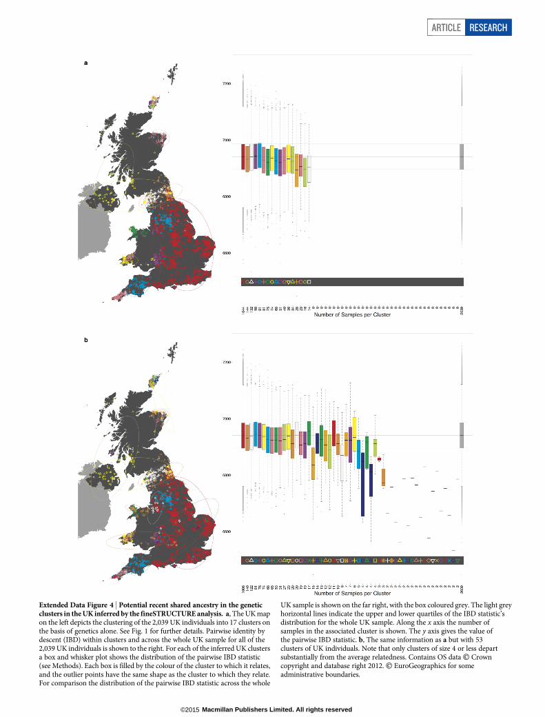
Extended Data Figure 4 | Potential recent shared ancestry in the geneticclusters in the UK inferred by the fineSTRUCTURE analysis. a, The UK mapon the left depicts the clustering of the 2,039 UK individuals into 17 clusters onthe basis of genetics alone. See Fig. 1 for further details. Pairwise identity bydescent (IBD) within clusters and across the whole UK sample for all of the2,039 UK individuals is shown to the right. For each of the inferred UK clustersa box and whisker plot shows the distribution of the pairwise IBD statistic(see Methods). Each box is filled by the colour of the cluster to which it relates,and the outlier points have the same shape as the cluster to which they relate.For comparison the distribution of the pairwise IBD statistic across the whole

UK sample is shown on the far right, with the box coloured grey. The light greyhorizontal lines indicate the upper and lower quartiles of the IBD statistic’sdistribution for the whole UK sample. Along the x axis the number ofsamples in the associated cluster is shown. The y axis gives the value ofthe pairwise IBD statistic. b, The same information as a but with 53clusters of UK individuals. Note that only clusters of size 4 or less departsubstantially from the average relatedness. Contains OS data E Crowncopyright and database right 2012. E EuroGeographics for someadministrative boundaries.

ARTICLE RESEARCH

Macmillan Publishers Limited. All rights reserved©2015

RESEARCH ARTICLE

Macmillan Publishers Limited. All rights reserved©2015

Extended Data Figure 5 | Population structure in the European samples.a, Number of samples derived from each European sampling region. The 6,209European samples used for the analyses were sampled from ten countries andvarious locations within each country. Each sample has a specific samplinglocation (often a city, but in some cases only a whole country). The numbersshown give the number of samples derived from a particular location.Some numbers are depicted out of position for clarity. In these cases a line leadsfrom the number to the actual location. Where the sample locationsare well-localized (for example, the city of sampling is known) the boxsurrounding the number is white. When only information about the country ofsampling is known the box is coloured yellow. The numbers are overlain on afaded version of the pie charts from panel b for easy reference. b, Europeanpopulation structure inferred by fineSTRUCTURE. The 6,209 Europeansamples divided into 51 genetic groups (represented by colours and labelledwith a subset of the numbers between 1 and 145) using fineSTRUCTURE. For

clarity the colour space has been skewed to emphasize the differencesbetween groups 1 to 18 as these groups are the major contributors to theancestry profiles of the UK clusters. Each sample has a specific samplinglocation (often a city, but in some cases only a country, see panel a). The piecharts are located at these sampling locations, and depict the proportion of thesamples from that location assigned to each of the 51 genetic groups.Each genetic group also has a label number, which is displayed for the largersectors of each of the pie charts. The area of the pie chart is proportional tothe number of samples from that location. Pie charts with black borderscorrespond to well-localized samples. In contrast, for samples where onlythe country of sampling is known, they are combined in a single pie chart forthe country, which is shown with white borders. Some pie charts aredepicted out of position for clarity; in these cases a line leads fromthe chart to the actual location. E EuroGeographics for theadministrative boundaries.

ARTICLE RESEARCH

Macmillan Publishers Limited. All rights reserved©2015

Extended Data Figure 6 | European ancestry profiles of the UK clusters.a, The map of the UK shown relates to the map with 17 UK clusters shownin Fig. 1. Ellipses indicate the extent of the UK clusters as in Fig. 1. The pie chartsrepresent the ancestry profile of the UK clusters from Fig. 1. Each pie chartis plotted at the centroid of the corresponding cluster, although some pie chartshave been moved for clarity; in the cases where the relocation is substantial a redline leads from the pie chart to the centroid. The sectors of the pie charts arecoloured with the colours of the European genetic groups (for the larger sectorsthe number of the European group is also given). They indicate the ancestryprofiles of each UK cluster, namely the proportion of the cluster ancestry that isbest represented by each of the European groups. The magnitude of the angle ofa sector is proportional to the contribution of that European group to theancestry profile of the associated UK cluster. The symbols in the grey bar to theleft of the map represent the UK clusters as in Fig. 1. The bar chart in the leftpart of the plot depicts the same ancestry profiles of the UK clusters in adifferent way. Each row represents a UK cluster (arranged roughly north tosouth) with the symbols for the clusters from Fig. 1 indicated at each end of the

row. Each column represents a European group, with group numbers listedwith a three letter prefix that, for clarity, relates to the country or countrieswhere the cluster is most represented. The colour of each bar also indicates theEuropean group to which the bar relates. Confidence intervals (95%) obtainedfrom 1,000 bootstraps of the ancestry profile analysis (see Methods) areindicated on each bar. b, Renormalized ancestry profiles of the UK clustersillustrating possible early European contributions to the UK population. Arepresentation of the relative contributions to the UK clusters from the threeEuropean groups (GER6-W. Germany, BEL11- Belgium, and FRA14-NWFrance) hypothesized to be the major contributors to the earliest migrationsinto the UK after the last ice age from which DNA survives to the present insubstantial proportions (see Supplementary Note). Interpretation of themap, pie charts and bar chart is as for a. In this case, however, the proportionswere renormalized to sum to 1 for the contributions from GER6, BEL11and FRA14. Contains OS data E Crown copyright and database right 2012.

E EuroGeographics for some administrative boundaries.

RESEARCH ARTICLE

Macmillan Publishers Limited. All rights reserved©2015

a

b

Extended Data Figure 7 | More major events in the peopling of the British Isles. See Supplementary Note for further details. a, The arrival of agriculture andsubsequent migrations from 4000–2500 BC. b, The major iron age tribes of Britain around the year 40. E EuroGeographics for the administrative boundaries(coastlines).

ARTICLE RESEARCH

Macmillan Publishers Limited. All rights reserved©2015

Extended Data Figure 8 | Application of GLOBETROTTER to infersimulation of ancestry 40 generations ago between groups from NorthernGermany (GER3, 25%) and Italy (ITA36, 75%). Twenty-five admixedindividuals were simulated, and the individuals used to construct thesesimulated individuals were then removed from the list of potential donors(see Methods). Left barplot, and map: the barplot shows the true populationand proportion contributed for each of the two admixing groups. The mapshows, for each of the European sampling locations, the true proportion ofindividuals sampled from that location assigned to each of the admixinggroups, coloured according to the barplot. Central three plots: example curvesconstructed by GLOBETROTTER to infer admixture times, and infer details ofadmixing groups (see Methods and Supplementary Note). For each pair ofpopulations A and B (A can be the same as or different from B) the points showthe empirical probability, relative to under independence, as a function ofgenetic distance x, that two positions separated by distance x correspond toancestry donated by population A, and by population B, respectively. The greenline shows GLOBETROTTER fitted exponential decay curves for theunderlying (that is, expected) value of this relative probability estimate. Undera model of a single admixture event occurring g generations ago, thisprobability decays at a rate g according to theory, providing an estimate ofthe admixture time (and 95% CI) shown overlaying the curve ITA36 versusGER3. If ancestries A and B associate with the same admixing group, forexample, whenever A 5 B the fitted curve will have a negative slope, as seen for

the GER3 versus GER3 plot. If a positive slope is seen, as for the ITA36 versusGER3 plot, this implies these populations contribute to the two differentrespective admixing groups. Right bar-plot, and map: GLOBETROTTERproduces an inference of the genetic composition of (haplotypes carried by) thetwo admixing groups, as a mixture of (haplotypes carried by) populationsactually sampled. This mixture inference jointly uses curves for pairs ofsampled populations, and the overall haplotypic makeup of different sampledpopulations, including the admixed group. The bar-plot shows the inferredmixture representation (dominated in each case by the true admixing groups)and estimated admixture proportion (24%, close to the truth of 25%), withmore red/blue populations respectively giving a larger contribution. The mapshows populations inferred as contributing to the first (pink/red shades) orsecond (blue shades) admixing group, respectively, as for the left map, withpopulations coloured according to the bar-plot. This shows populations falselyinferred as contributing material to the admixing groups were still sampled,mainly, from locations close to those of the true admixing groups. Wecaution that in this setting of admixture between genetically similarEuropean groups, estimation of admixture fraction is very uncertain (seeMethods) (for example, contributing populations are often impossible todefinitively assign to a ‘side’ of the event). For further details of the analysis,for example, tests for admixture presence in this simulation, seeMethods and Supplementary Note. E EuroGeographics for theadministrative boundaries.

RESEARCH ARTICLE

Macmillan Publishers Limited. All rights reserved©2015

ARTICLE RESEARCH

Macmillan Publishers Limited. All rights reserved©2015

Extended Data Figure 9 | Application of GLOBETROTTER to infer detailsof admixture in the UK clusters. a, Inferring admixture in a population of1,044 UK individuals from central and southern England. Left hand plot: thebold red squares show mean grandparental birthplace for each individualin this cluster. Central three plots: example curves constructed byGLOBETROTTER to infer admixture times, and infer details of admixinggroups (see Methods and Supplementary Note). For each pair of populationsA and B (A can be the same as or different from B) the points show theempirical probability, relative to under independence, as a function of geneticdistance x, that two positions separated by distance x correspond to ancestrydonated by population A, and by population B, respectively. The green lineshows GLOBETROTTER fitted exponential decay curves for the underlying(that is, expected) value of this relative probability estimate. Under a modelof a single admixture event occurring g generations ago, this probability decaysat a rate g according to theory, providing an estimate of the admixture time(and 95% CI) shown overlaying curves SFS31 versus GER3 and SFS31 versusSFS31. If ancestries A and B associate with the same admixing group, forexample, whenever A 5 B the fitted curve will have negative slope, as seen forthe GER3 versus GER3 plot. If a positive slope is seen, as for the SFS31 versusGER3 plot, this implies these populations contribute to the two differentrespective admixing groups. Right bar-plot, and map: GLOBETROTTERinference shows one possibility for the genetic composition of (haplotypescarried by) the two unsampled historical admixing groups, as a mixture of(haplotypes carried by) populations actually sampled. This mixture inferencejointly uses curves for pairs of sampled populations, and the overall haplotypicmakeup of different sampled populations, including the admixed group. Thebar-plot shows the inferred mixture representation (with largest contributionsin each case by GER3/DEN18, sampled most frequently from northernGermany and Denmark, and SFS31/ITA52, sampled mainly from southernFrance and Spain and northern Italy) and estimated admixture proportion(34%), with more intense red/blue populations respectively implying a largercontribution. The map shows populations inferred as contributing to the first(pink/red shades) or second (blue shades) admixing group respectively, withpopulations coloured according to the bar-plot. We caution that in this settingof admixture between genetically similar European groups, estimation ofadmixture fraction is very uncertain (see Methods and Supplementary Note)(for example, contributing populations are often impossible to definitivelyassign to a side of the event), so that other closely related scenarios, for example,a somewhat lower admixture fraction from a more completely ‘GER3’-likegroup than that inferred, are likely consistent with the GLOBETROTTERresults seen. b, Inferring admixture in a population of 51 UK individuals fromOrkney. Left hand plot: the bold purple squares show mean grandparental

birthplace for each individual in this cluster. Central three plots: example curvesconstructed by GLOBETROTTER to infer admixture times, and infer details ofadmixing groups (see Methods and Supplementary Note). For each pair ofpopulations A and B (A can be the same as or different from B) the points showthe empirical probability, relative to under independence, as a function ofgenetic distance x, that two positions separated by distance x correspond toancestry donated by population A, and by population B, respectively. The greenline shows GLOBETROTTER fitted exponential decay curves for theunderlying (that is, expected) value of this relative probability estimate.Under a model of a single admixture event occurring g generations ago, thisprobability decays at a rate g according to theory, providing an estimate of theadmixture time (and 95% CI) shown overlaying curves NOR90 versus FRA12and NOR90 versus NOR90. If ancestries A and B associate with the sameadmixing group, for example, whenever A 5 B the fitted curve will havenegative slope, as seen for the NOR90 versus NOR90 plot. If a positive slope isseen, as for the NOR90 versus FRA12 plot, this implies these populationscontribute to the two different respective admixing groups. Right bar-plot, andmap: GLOBETROTTER inference shows one possibility for the geneticcomposition of (haplotypes carried by) the two unsampled historical admixinggroups, as a mixture of (haplotypes carried by) populations actually sampled.This mixture inference jointly uses curves for pairs of sampled populations,and the overall haplotypic makeup of different sampled populations, includingthe admixed group. The bar-plot shows the inferred mixture representation(with largest contribution in each case by GER3/NOR90, sampled mostfrequently from northern Germany and Norway, and FRA12/FRA14, bothsampled mainly from France) and estimated admixture proportion (42%), withmore intense red/blue populations respectively implying a larger contribution.The map shows populations inferred as contributing to the first (pink/redshades) or second (blue shades) admixing group respectively, with populationscoloured according to the bar-plot. We caution that in this setting of admixturebetween genetically similar European groups, estimation of admixturefraction is very uncertain (see Methods and Supplementary Note) (for example,contributing populations are often impossible to definitively assign to a ‘side’of the event). In particular, inspection of curves involving GER3 does notyield a clear ‘side’ of the event for this population, unlike the NOR90 versusFRA12 case that implies French-like and Norwegian-like haplotype presencemust occur mainly in distinct admixing groups. Therefore the GER3component might in fact capture haplotypes for either (or both) the French-likeor Norwegian-like admixing groups, and the inferred scenario shows onlyone possibility. Contains OS data E Crown copyright and database right 2012.

E EuroGeographics for some administrative boundaries.

RESEARCH ARTICLE

Macmillan Publishers Limited. All rights reserved©2015