Genetic Regulatory Network Models of Biological Clocks: Evolutionary History Matters

Genetic Regulatory Network models of Biological Clocks:

Evolutionary history matters

Johannes F. Knabe1 Chrystopher L. Nehaniv1,2

Maria J. Schilstra2

Adaptive Systems1 and BioComputation2 Research Groups,

University of Hertfordshire, Hatfield AL10 9AB, UK

{j.f.knabe, c.l.nehaniv, m.j.1.schilstra}@herts.ac.uk

“For three billion years, [...] life here has grown and adapted, passing form cell to cell innumer-

able times in unbroken descent, generation after generation[, ...] we’ve felt the sky brighten and

darken again and again while the planet relentlessly rotated: a trillion cycles of brightness and

dark, of warmth and chill, never missing a beat, always felt deep in the chemical essence of what

we are. What would a trillion cycles sound like? Like high C for 400 years. [... If we] venture out

among the stars, we still hum with the pitch of our homeland. Anyone we meet out there will know

where we came from, not just by our carbon and our water and thecolors we see best, but also by

the approximate 24-hour pitch of all that we do.” – Arthur T. Winfree [31, p. 5]

Abstract

We study the evolvability and dynamics of artificial geneticregulatory networks (GRNs), as active control

systems, realizing simple models of biological clocks thathave evolved to respond to periodic environmental

stimuli of various kinds with appropriate periodic behaviors.

GRN models may differ in the evolvability of expressive regulatory dynamics. A new class of artificial

GRNs with an evolvable number of complex cis-regulatory control sites – each involving a finite number of

inhibitory and activatory binding factors – is introduced,allowing realization of complex regulatory logic.

1

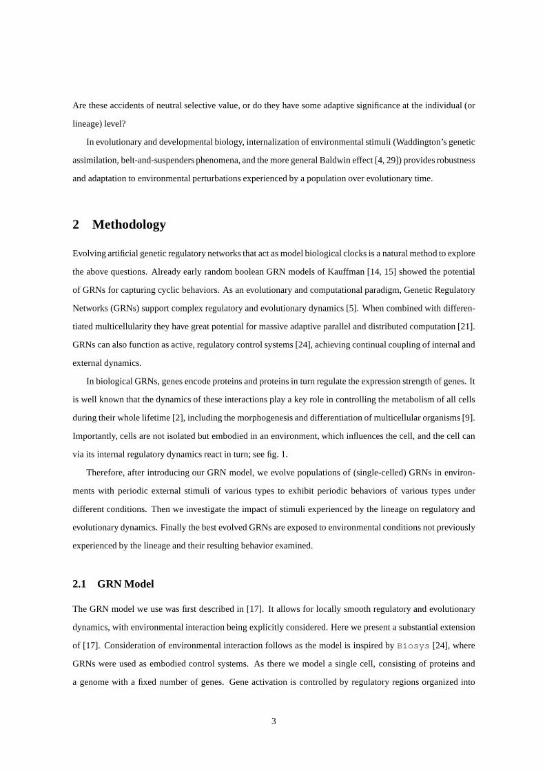
Previous work on biological clocks in nature has noted the capacity of clocks to oscillate in the absence

of environmental stimuli, putting forth several candidateexplanations for their observed behavior, related to

anticipation of environmental conditions, compartmentation of activities in time, and robustness to perturba-

tions of various kinds, or unselected accidents of neutral selection. Several of these hypotheses are explored

by evolving GRNs with and without (gaussian) noise and “black out periods” for environmental stimulation.

Robustness to certain types of perturbation appears to account for some, but not all, dynamical properties of

the evolved networks. Unselected abilities, also observedfor biological clocks, include the capacity to adapt

to change in wavelength of environmental stimulus, and to clock resetting.

Keywords: Biological Clocks, Genetic Regulatory Networks (GRNs), Baldwin Effect, Environmental Cou-

pling, Phase Resetting, Evolutionary Algorithms

1 Biological Clocks

A characteristic of life on earth is itsincessant responsiveness[29]. Not all organismal responses to external

stimuli are simple reactive responses, but behavior generally depends also on the organism’s internal state –

and this state can reflect environmental processes. Biological clocks provide one of the simplest yet most

characteristic examples of such internalized incessant responsiveness for life as it has evolved on the earth in

that an organism’s regulatory dynamics respond with periodic activity in close coupling with periodic cycles

of environmental stimuli as experienced in the rhythm of light and dark, or in the effects of lunar gravitation in

the ebb and flow of tides.

Biological systems exhibit periodic behavior on differenttime scales, but circadian rhythms are believed

to have originated already in the earliest cells. The atmosphere on early earth allowed much higher ultraviolet

radiation to penetrate during day-time, and nightly cell division provided protection for replicating DNA. This

replication behavior can, for example, today still be foundin the single-celled organismGonyaulax polyedra

[31].

Without the capacity to adjust to external signals, minute differences in timing period soon accumulate,

leading to internal clocks being hopelessly out of step withthe environment.

Following Winfree [30, 31], one may ask, How is it that biological clocks still work when external stimuli

are hidden (like the sun or other temporal cues) in isolationexperiments on living organisms? How is it that

they can adapt, within limits, to perturbations in cycle length, phase shift, and resetting? Why in isolation do

they run at rates somewhat different from that of the external cycles (with rates being species specific; while the

aforementionedGonyaulaxhas an internalized rhythm of roughly 23 hours, humans are closer to 25 hours)?

2

Are these accidents of neutral selective value, or do they have some adaptive significance at the individual (or

lineage) level?

In evolutionary and developmental biology, internalization of environmental stimuli (Waddington’s genetic

assimilation, belt-and-suspenders phenomena, and the more general Baldwin effect [4, 29]) provides robustness

and adaptation to environmental perturbations experienced by a population over evolutionary time.

2 Methodology

Evolving artificial genetic regulatory networks that act asmodel biological clocks is a natural method to explore

the above questions. Already early random boolean GRN models of Kauffman [14, 15] showed the potential

of GRNs for capturing cyclic behaviors. As an evolutionary and computational paradigm, Genetic Regulatory

Networks (GRNs) support complex regulatory and evolutionary dynamics [5]. When combined with differen-

tiated multicellularity they have great potential for massive adaptive parallel and distributed computation [21].

GRNs can also function as active, regulatory control systems [24], achieving continual coupling of internal and

external dynamics.

In biological GRNs, genes encode proteins and proteins in turn regulate the expression strength of genes. It

is well known that the dynamics of these interactions play a key role in controlling the metabolism of all cells

during their whole lifetime [2], including the morphogenesis and differentiation of multicellular organisms [9].

Importantly, cells are not isolated but embodied in an environment, which influences the cell, and the cell can

via its internal regulatory dynamics react in turn; see fig. 1.

Therefore, after introducing our GRN model, we evolve populations of (single-celled) GRNs in environ-

ments with periodic external stimuli of various types to exhibit periodic behaviors of various types under

different conditions. Then we investigate the impact of stimuli experienced by the lineage on regulatory and

evolutionary dynamics. Finally the best evolved GRNs are exposed to environmental conditions not previously

experienced by the lineage and their resulting behavior examined.

2.1 GRN Model

The GRN model we use was first described in [17]. It allows for locally smooth regulatory and evolutionary

dynamics, with environmental interaction being explicitly considered. Here we present a substantial extension

of [17]. Consideration of environmental interaction follows as the model is inspired byBiosys [24], where

GRNs were used as embodied control systems. As there we modela single cell, consisting of proteins and

a genome with a fixed number of genes. Gene activation is controlled by regulatory regions organized into

3

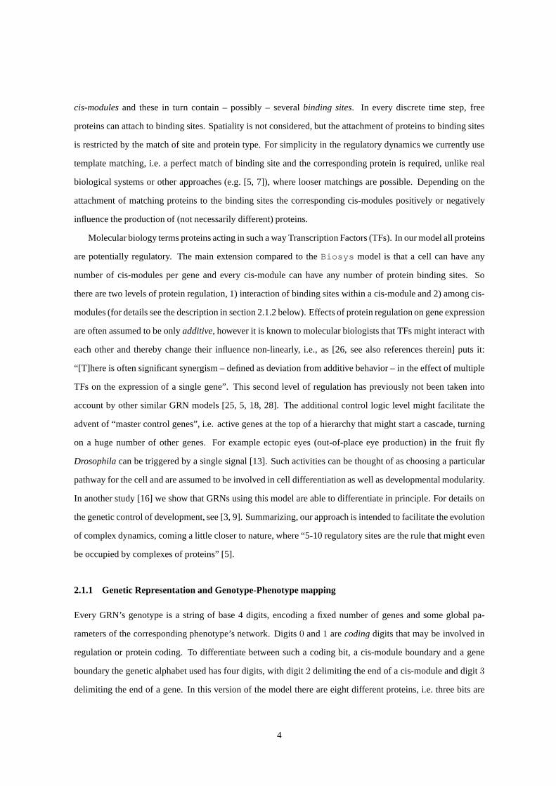
cis-modulesand these in turn contain – possibly – severalbinding sites. In every discrete time step, free

proteins can attach to binding sites. Spatiality is not considered, but the attachment of proteins to binding sites

is restricted by the match of site and protein type. For simplicity in the regulatory dynamics we currently use

template matching, i.e. a perfect match of binding site and the corresponding protein is required, unlike real

biological systems or other approaches (e.g. [5, 7]), wherelooser matchings are possible. Depending on the

attachment of matching proteins to the binding sites the corresponding cis-modules positively or negatively

influence the production of (not necessarily different) proteins.

Molecular biology terms proteins acting in such a way Transcription Factors (TFs). In our model all proteins

are potentially regulatory. The main extension compared totheBiosys model is that a cell can have any

number of cis-modules per gene and every cis-module can haveany number of protein binding sites. So

there are two levels of protein regulation, 1) interaction of binding sites within a cis-module and 2) among cis-

modules (for details see the description in section 2.1.2 below). Effects of protein regulation on gene expression

are often assumed to be onlyadditive, however it is known to molecular biologists that TFs might interact with

each other and thereby change their influence non-linearly,i.e., as [26, see also references therein] puts it:

“[T]here is often significant synergism – defined as deviation from additive behavior – in the effect of multiple

TFs on the expression of a single gene”. This second level of regulation has previously not been taken into

account by other similar GRN models [25, 5, 18, 28]. The additional control logic level might facilitate the

advent of “master control genes”, i.e. active genes at the top of a hierarchy that might start a cascade, turning

on a huge number of other genes. For example ectopic eyes (out-of-place eye production) in the fruit fly

Drosophilacan be triggered by a single signal [13]. Such activities canbe thought of as choosing a particular

pathway for the cell and are assumed to be involved in cell differentiation as well as developmental modularity.

In another study [16] we show that GRNs using this model are able to differentiate in principle. For details on

the genetic control of development, see [3, 9]. Summarizing, our approach is intended to facilitate the evolution

of complex dynamics, coming a little closer to nature, where“5-10 regulatory sites are the rule that might even

be occupied by complexes of proteins” [5].

2.1.1 Genetic Representation and Genotype-Phenotype mapping

Every GRN’s genotype is a string of base 4 digits, encoding a fixed number of genes and some global pa-

rameters of the corresponding phenotype’s network. Digits0 and1 arecodingdigits that may be involved in

regulation or protein coding. To differentiate between such a coding bit, a cis-module boundary and a gene

boundary the genetic alphabet used has four digits, with digit 2 delimiting the end of a cis-module and digit3

delimiting the end of a gene. In this version of the model there are eight different proteins, i.e. three bits are

4

sufficient to code for the protein type.

After parsing the genome into genes, the last four coding digits of every gene determine its output behavior.

Three bits for the protein produced and the last bit for the gene’s activation type, which can beconstituitive

(“default on”) or induced(“default off”).

The first coding bit of a cis-module determines its influence on the gene’s activation level (inhibitory/activatory)

and every following three coding digits are considered a TF binding site.

Note that, due to evolutionary operators explained below, there might be additional digits that are not

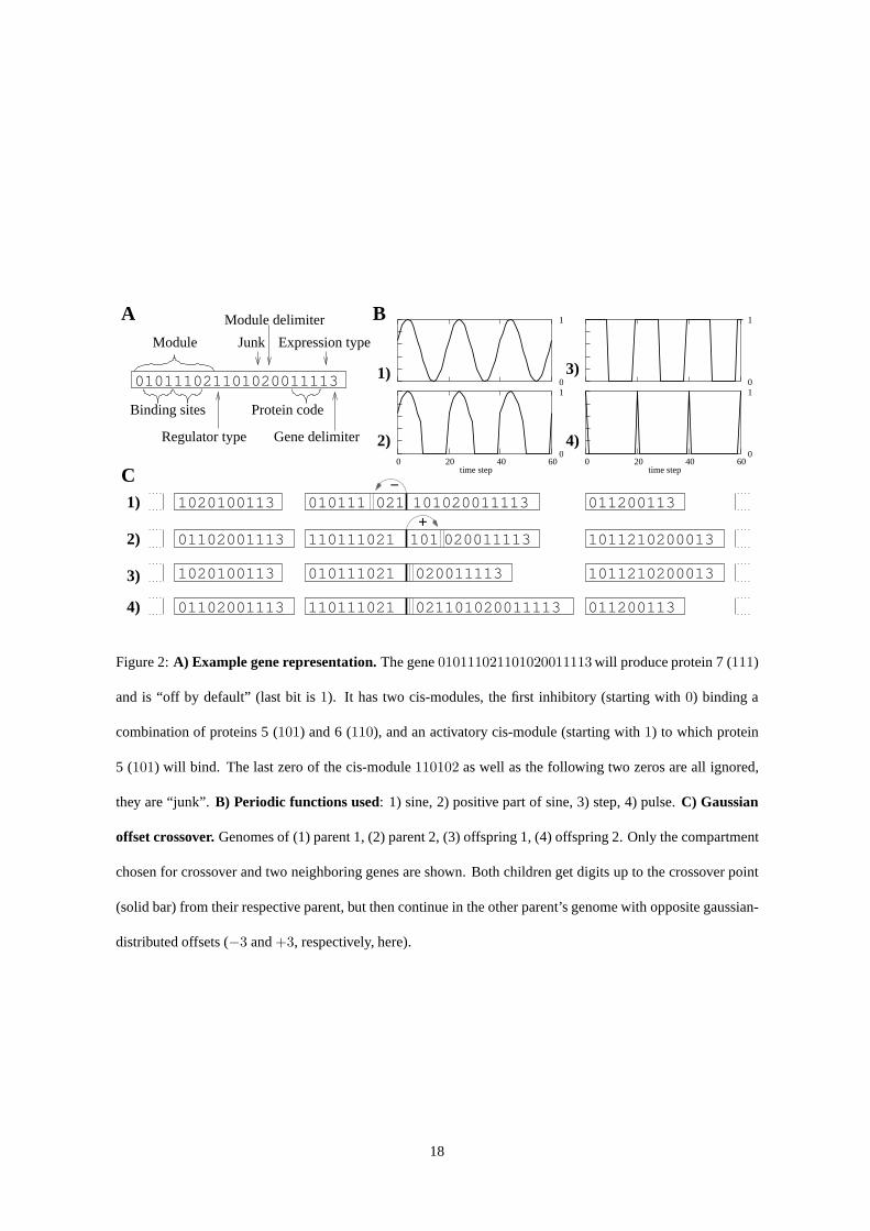
meaningful.We refer to such digits which are neither translated nor regulatory asjunk. See fig. 2 A) for an

example gene representation.

The genome also encodes several evolvable variables globalto the cell. These are 1) theprotein-specific decay

rates, four bits for each of the eight protein types, indexing intoa fixed lookup table of values, 2) the global

binding proportion, also four bits indexing into a lookup table, but identical for all proteins, and finally 3) the

globalsaturation value, three bits indexing to look up table the same for all proteins.

2.1.2 Regulatory Logic

A GRN is run over a series of discrete time steps, its lifetime. In every time step initially a fraction of the

free proteins, determined by the global binding proportionparameter, are bound to matching sites. In this

process all protein binding sites are treated equally, regardless of the cis-module to which they belong. To

determine the output of every gene, within each cis-module the minimum of bound protein over all binding

sites is first calculated. Note that this use ofmin is an extension of logicalAND and results in non-additive

effects (“synergy”) in gene regulation. Furthermore this is a canalizing function in the sense of Kauffman [15],

who underlines their importance for dynamical properties of boolean networks. For a function to be canalizing

(at least) one input variable must be able to assume a value that forces a certain output value, regardless of

the other inputs – which is clearly the case here as one low input to themin function suffices to ensure a low

output. In a second step the sum of the minima of these cis-module values is taken, with inhibitory modules

having a negative sign. Finally this activation level is passed to an either constituitive or induced sigmoid

threshold activation function for the gene. For reasons of space full details can not be given here but can

be found in [1, 17]. The output of the gene’s activation function is added to the unbound concentration of

that gene’s output protein type. Afterwards the concentrations of all unbound proteins are checked for being

above the global saturation value and all proteins, free or bound, decayed by the protein specific rate. Finally,

environmental input to the GRN-controlled cell can occur byincreasing the unbound concentration of certain

5

proteins by some value and output by reading some protein concentration values.1

2.2 Evolution

We use a standard Genetic Algorithm with elitism, tournament selection and replacement. Every evolutionary

condition was studied with ten runs of 500 generations with apopulation size of 250 individuals, where one

individual consisted of a single cell with GRN-controlled interaction with its environment as determined by

its genome and regulatory dynamics. The initial populationstarted with one cis-module per gene and one

protein binding site per cis-module, all coding bit values being randomly assigned – with a fixed number of

genes during evolution. In network terms, depicting genes as nodes and protein products of a gene that match

a binding site of another gene as arcs between those nodes2, the nodes are randomly connected, with at most

one incoming arc.

2.2.1 Selection

Later generations are formed by carrying over the best-performing individual of the last generation automati-

cally and, keeping population size constant, the other individuals are replaced by offspring. For every pair of

offspring, 15 (not necessarily different) individuals of the prior generation are chosen randomly and of these

the best two selected to be “parents”.

2.2.2 Variability

Going from parent genomes to offspring, recombination by a (single-point) crossover is applied with a prob-

abilty of 0.9. Additionally mutation is used on offspring genomes, everycoding bit (not delimiters) is flipped

with a probability of one percent. To generate a variable number of cis- and of protein binding sites per gene it

is necessary to have variable length genomes. Note that despite this, the number of genes stays the same all the

time. These properties are achieved by dividing the parent genomes into compartments: one compartment for

every gene and one compartment for the global variables. Then (with a probability of 0.9) a single compart-

ment is chosen for crossover and in this compartment a point allocated for crossover. However when crossing

over from parent 1’s genome to the second parent’s genome copying does not necessarily continue at the same

position of parent 2’s genome but is shifted by an offset (gaussian offset crossover – see fig. 2 C), mimicking

1Simple scaling is used to map stimulus input levels from the signal range to a protein concentration, andvice versafor output protein

levels.2Another possibility would be to visualize such a network using protein types as nodes with arcs going from every binding site protein

type that a gene has to the gene’s output protein.

6

the unequal crossing-over observed in biology [12].

This offset is randomly drawn from a gaussian distributed random variable with mean zero and standard

deviation four. The relatively large number four was chosento allow for some shifts by three to occur. An

offset of three is likely to add/remove exactly one binding site and at most disturb immediately adjoining sites.

Other values are more likely to cause a change in the reading frame, i.e. all following binding sites change

the protein type they are receptive for – very much like what biologists call a frameshift mutation. In network

terms the latter can have a huge impact on the GRN’s dynamics while the former might yield a relatively smooth

transition. The importance of duplicating genetic information was already pointed out by [23] for the evolution

of biological complexity – see also [22, 20]. Ohno put emphasis on whole-genome duplications while it is now,

with better techniques, becoming ever clearer that “both small- and large-scale duplication events have played

major roles” [27, p. 320]. Experiments where the duplication of whole genes is possible, in network terms the

addition of nodes with the same connection structure as an existing node, are underway.

Note that the offset point is limited to stay within the boundaries of the compartment, hence if crossover point +

offset is smaller/larger than the left/right boundary it isset to the corresponding boundary value. So the number

of 2s (cis-modules) might increase by crossover – mutation was only applied to coding digits – but not the

number of 3s as these are the compartment boundaries. When crossover occurs in the part encoding for global

parameters the offset is always set to 0 as offsets would be meaningless here.

These processes allow both neutral crossover and mutational changes, as degenrate cis-modules (i.e. less than

three bits – one protein encoding – long) are ignored. Additionally this means that, although the number of

genes was constant over one evolutionary run, genes could become inactive, in a manner similar to the so-called

pseudo-genes found in nature, i.e. if they have no non-degenrate cis-module and the gene has activation type

“off by default”.

To check how useful exchange of genetic material in the creation of new individuals is for our problem, we

also ran one condition where only the single best individualof the group of 15 was chosen as parent. Its

genome would then be crossed over with itself as described above – so none of the properties of offspring

generation mentioned is lost. However chances are then muchhigher that offspring regulatory dynamics (and

thereby performance) are not too different from the parent’s as most genes could be crossed only with identical

copies of themselves. So we have, in effect, reduced the variability likely yielding smoother transitions for this

self-crossovercondition.

7

2.3 Environmental Coupling

As stated in the introduction, environmental cycles have a huge impact on the life of organisms on earth. But

in what way these stimuli affect an active organism via its signal transduction pathways and what behavior is

appropriate depends on the type of organism. Here we systematically vary evolutionary conditions by varying

the periodic pattern of external signal received at the cellular level — in some scenarios distorted or interrupted

or both — as well as the periodic output behavior expected. Asa control condition we also tested what

performance could be achieved without any external signalsever. Experimental variations included whether

input and target output were in the same or fixed shifted phase, and whether GRNs were started in a random

phase.

2.3.1 Input stimuli

The basic idea was to have periodic environmental stimuli based on a sine curve (shifted to the interval[0, 1]).

The wavelength was set to 20 time steps, while the lifetime for every GRN was 400 steps. Variations included

having only the positive part of sine, a periodic step function, and a brief pulse. The four functions used are de-

picted in fig. 2 B). In addition, we varied whether gaussian noise or “black-outs”, periods of no external signal,

were applied, yielding four further conditions:[±noise,±blackout]. In [−noise,−blackout] scenarios, the

input signal was transduced to yield a corresponding input of a particular protein as described above, without

any distortion. In a[+noise] condition, gaussian white noise with a standard deviation of 0.1 was added to

model imperfect signal transduction.3 For [+blackout] conditions, at random points in time the input stopped

completely for an interval of time: every GRN experienced two periods at random times without input, each

lasting for 5 percent of its lifetime. In the[+noise,+blackout] scenarios, these perturbations were combined

(with the black-out being stronger than the noise, so there was no input – not even noise – during black-out

periods).

2.3.2 Output behavior

Two periodic target functions were used to measure the performance of an individual and assign fitness: sine

(fig. 2 B.1) and step (fig. 2 B.3). As stated above, the target output’s shape and phase might differ from the

input, however the wavelength was always the same. Fitness was measured based on the deviation from this

target output, i.e. the smaller the value, the better adapted the GRN.

Letting ct

i0denote the (unbound) concentration of the GRN’s output protein i0 anddt the target output at time

t the overall deviation is simply calculated as:D =∑L

t=1|ct

i0−dt|. The lifetimeL of every individual was set

3Note however that values below zero are set to zero as negative protein input is not possible.

8

to 400 time steps. A randomly-generated initial GRN could typically achieve a deviation of approximately 200.

Finally, we use this value to transform the deviation to a standard 0 to 100 performance scale:(200−D)/2, so

zero deviation would result in a perfect performance value of 100.

2.4 Experimental Scenarios

Overall 32 evolutionary conditions were tested (two targetoutput types times four environmental stimulus input

functions in four environmental coupling variations each,as described above) and every condition was run ten

times. Additionally the number of genes was varied (see below). To test the results for robustness, the complete

set of experiments was run in four variations denoted as follows:

[0]: Always starting in a fixed phase, with no shift between inputand target output phase.

[ 12]: Starting in a fixed phase, but with a phase shift of1

2period between input and target output.4

[r]: Starting in a random phase for each individual, with no shift between input and target output phase.

[ 12

+ r]: Combining[ 12] and[r], i.e. shifting the input’s phase by half the wavelength plusa random number

while shifting the output’s phase by that random number only.

Also, [∅] denotes no environmental input ever and[s] the self-crossover condition.

To test how the evolved GRNs were affected by their evolutionary history we also put the best ones into envi-

ronments not experienced by them or their ancestors before.At first, they got perturbed stimuli, i.e. variations

of their usual input functions with noise and/or black-outsunlike the evolutionary history of their lineage. Af-

terwards special new stimuli were used: constant input, phase shifted input, different wavelength input, or very

long blackout periods.

3 Results

In almost every single run well adapted GRNs evolved, see table 1 (and [1]). Several individuals even achieved

deviation below 1 in some of the[−noise,−blackout] conditions.

We present a selection and summary of the most important results here, detailed tables for all conditions,

with lifetime graphs of GRN behaviors can be found at http://panmental.de/GRNclocks. The first subsection

examines how populations evolved and the average performances achieved; here we make a general compar-

ison between different scenarios. In the second subsectionthe focus of investigation shifts to the individual

regulatory dynamics, especially as observed in well adapted GRNs.

4Experiments with phase shifts of14

and 3

4have also been run, but as they are not qualitatively different and for reasons of space we

only give the results online, at http://panmental.de/GRNclocks.

9

3.1 Evolutionary Dynamics

Due to junk as well as inactive genes and binding sites, we could observe neutral changes, i.e. despite the

fact that performance often stayed the same for some evolutionary period, genome length might change during

crossover, or bits without function might be flipped. Although when crossing over with an offset different

from zero usually both a shorter and a longer descendants areproduced, the average population genome length

increases over evolutionary time. The amount of junk also increases, though at a slower rate, see [1] for data.

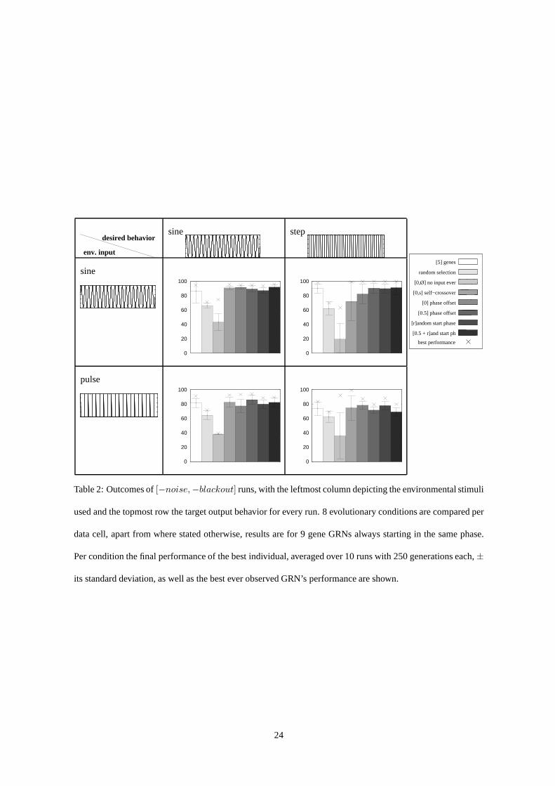
Running the same set of experiments with a fixed number of 5 genes and with 9 genes it turned out that the

ones with 9 genes in most cases ended up with a performance superior to their 5-gene equivalents (cf. table

2). In the tables and in the following text we always refer to 9gene GRNs if not mentioned explicitly, 5 gene

results are available online on the page mentioned above.

Examining the [0, ∅] results shown in table 2 it is not hard to see that GRNs are at abig disadvantage when they

never get any input stimuli from the environment – so one might conclude that it is hard or even impossible to

find regulatory dynamics that do not rely on external information to a certain degree. However in one condition

a GRN was identified that had access to external stimuli but ignored it while still performing well (see below

for details). Knowing this we found that, when well evolved GRNs from conditions with input were evolved a

little further in an environment without input, some of themwere able to return to a performance level similar

to the one they had when input was present within 10 generations. Apparently evolution was progressing faster

with some “perception” of the environment by the lineage.

Comparing the [0] with the [0, s] condition results, self-crossover performs worse in 7 outof 8 conditions. At

least for the problem at hand we can conclude that higher variability due to the mixing of genomes outperforms

presumably smoother self–crossover. Of course this will always depend on the structure of the search space

and how exploitative exploration shall proceed.

As mentioned before, in the reference case [0]with no phase shift and 9 genes, final GRNs performed reasonably

well, and at least one GRN did not use environmental input at all. With shifted input stimuli, condition[ 12],

the outcomes were generally comparable to the reference condition. So inverted patterns can be easily created

as output and performance is almost as good as without the phase shift. When starting in a random phase

(condition[r]) well adapted GRNs were of course forced to use external stimuli at least once to synchronize

with the environment – but still the rhythm (usually with a shorter period, though) was internalized in most

cases. The resulting performance was only slightly worse and in some conditions even better than in the

reference condition [0]. The same holds for a combination of the above variants (condition [ 12

+ r]).

10

3.2 Evolved Regulatory Dynamics

In all scenarios evolved GRNs exhibited a close match to the target output profile and almost always relied on

external signals to produce this behavior. As an exception,the best performing 9-gene GRN evolved with pulse

input (fig. 2.B.4) distorted by noise and black-outs to produce a step output had no binding sites for the input

protein, i.e. it did not rely on environmental stimuli at all. Apparently the regulatory logic was in principle able

to generate a close match to that target output without any external stimuli when every individuals’ lifetime al-

ways began at exactly the same phase. However the evolution of such dynamics was rare and it is probably not

a coincidence that this happened under the evolutionary conditions where only the starting phase was reliable.

Complex interaction networks evolved and all the best evolved GRNs made use ofAND-like regulatory

logic with several binding sites bundled to a cis-module as described above (an example of a 5-gene GRN is

shown in figure 3), although the initial random nets started with only one site per module. Examining the best

performing GRNs we found that their network structure, on average, with the genes as nodes and the binding

sites as incoming connections, was similar to scale-free networks. That is, there were few hubs with a high

in-degree while most nodes got little input (see fig. 4). Manyreal-world networks have the property of being

scale free, see [6]. For instance “the observed distributions in most genetic regulatory networks (for example

theE. coli network) are scale free for incoming links” [19].

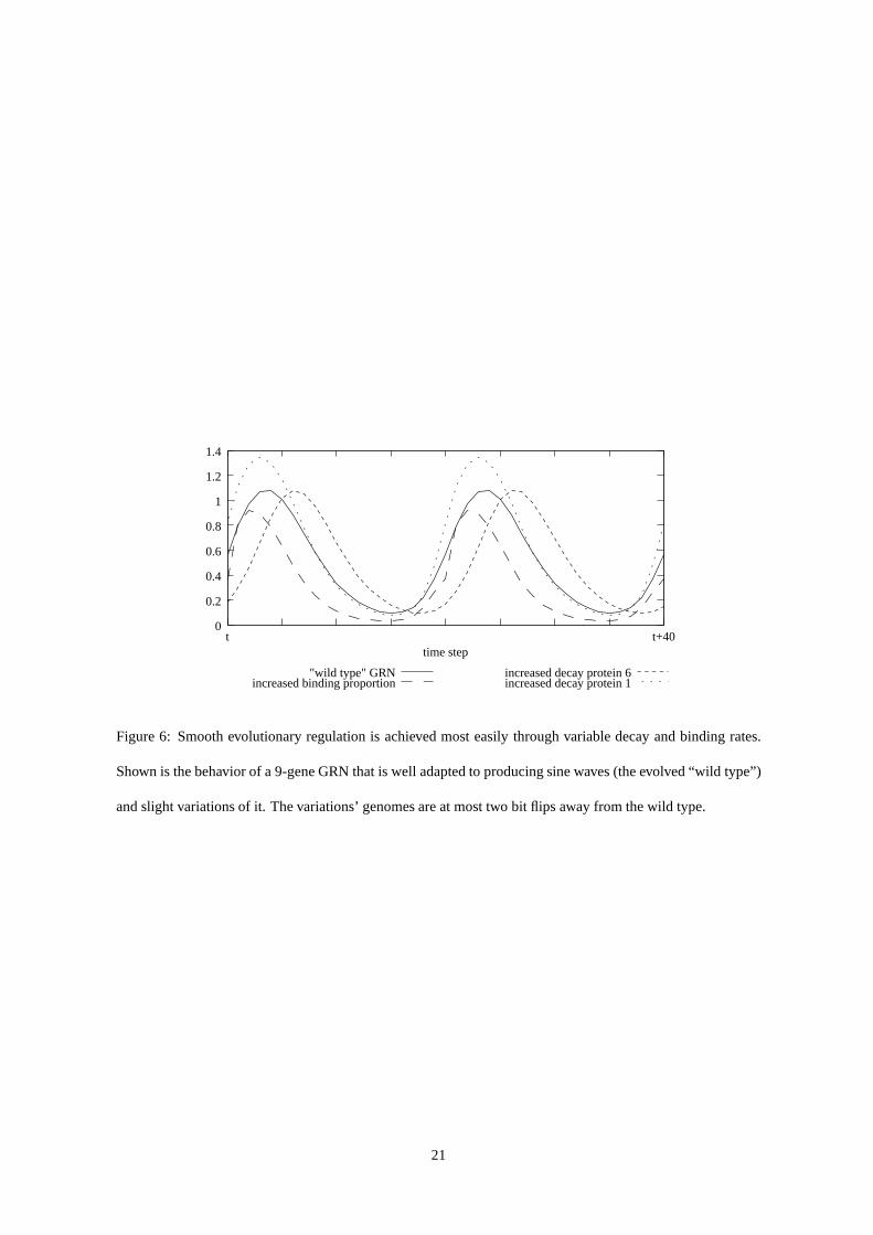
3.2.1 Smooth evolutionary regulation and Heterochrony

Smooth evolutionary regulation, i.e. changes in the timingof gene expression without affecting the general

dynamics, is achieved by varying protein decay rates and thebinding proportion (cf. fig. 6). The achievability

of similar phenomena in GRN models has also been demonstrated in [5]. Its importance for evolution in

the timing of developmental control, usually more specifically referred to as heterochronic control, has been

appraised by biologists, see e.g. [11], [8, p. 105].

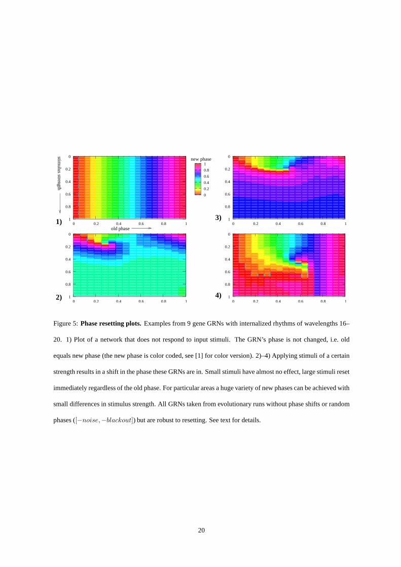
3.2.2 Phase Resetting

Again inspired by Winfree’s work [31] we also analyzed the phase resetting behavior of the evolved GRNs.

Organisms, deprived of their usual environmental clues to phase (e.g. dark room), usually follow some inter-

nalized rhythm instead. This however can be disturbed by giving stimuli (e.g. flash of light) – the rhythm

continues afterwards, but may be at another point in its cycle. Systematically done, we can for an interval of

old phases the organism is in, apply stimuli of different strength and record the resulting new phase. To map

11

this data on a 2D plot, the axes are for old phase and stimulus strength, while the important representational

trick is to code the new phase in color. As the color circle is cyclic (without sharp boundaries or discontinuity)

it can be repeated smoothly like a wave. For our GRNs with internalized rhythm (see next subsection), instead

of exposing them to some periodic stimulus, an input with a length of five time steps was applied at a particular

phase of their cycle (old phase) and then the new phase recorded. While resulting phase resetting plots showed

diverse structure, we discuss some of the typically exhibited features. These are illustrated by example plots,

see fig. 5. Easy to understand is the behavior with a very weak stimulus: the phase stays the same, we observe

no change. For very strong stimuli, the internal oscillatoris harshly reset – we also find a shift to the same

phase, regardless of the phase before the input stimuli was given. Most interestingly what we find in between

for medium strength stimuli is not always a smooth gradient between these extremes. We often observed that in

a small stimulus strength interval from a particular old phase almost every new phase could be reached. Given

continuous regulatory dynamics and environmental input, such a singularity necessarily must occur for purely

mathematical, topological reasons [31, ch. 4].

3.2.3 Behavior in Evolutionarily New Conditions

In what way and how strongly the evolved GRNs relied on input from the environment turned out to depend

strongly on the conditions under which they evolved (the evolutionary history of their lineage).

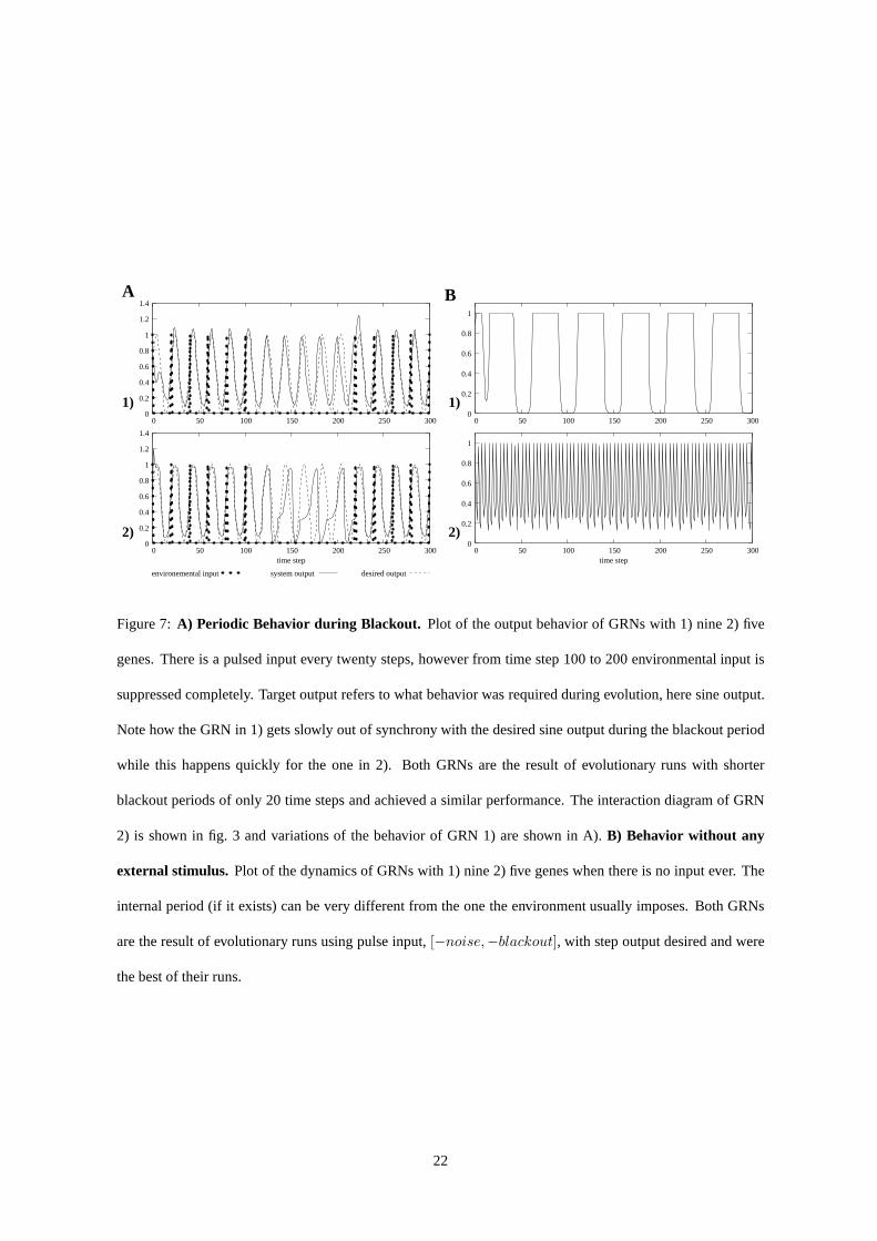
Internalized Rhythms When input stimuli were hidden, GRNs often exhibited an internalized output wave-

length different from the one which was the target during evolution, with some behaviors being quasiperiodic,

i.e. almost but not exactly retracing their paths through phase space. Such behavior occurred mainly in GRNs

evolved under pulse input, where the systems used the occasional input to stay synchronized, see fig. 7.A).

Apart from fast oscillations we observed systems with internal periods of varying length from 16 to almost 50

time steps (fig. 7.B.1).

Unselected Dynamical Properties Like most biological clocks studied in man and nature [31], nearly all the

best evolved GRNs – except those that completely ignored their input (which arose seldom and in only one

scenario) – in the various scenarios were robust to the shifts in phase and limited changes in wavelength of

periodic environmental stimuli. Wavelengths of 19 or 21 mostly did not pose problems, only higher deviations

from the normal cycle length of25% or more led to distorted outputs. Shifts in phase, i.e. when the input

stimulus immediately jumped to another point of the cycle, were tolerated by the evolved GRNs without trouble

at all. This occurs despite their lineage never having experienced such perturbations, i.e. without any selection

for these capabilities.

12

When GRNs evolved without noise (and/or black-outs) were placed in an environment with noise (and/or

black-outs), performance was still good, however – unsurprisingly – always worse than that of GRNs evolved

for such environments.

4 Discussion

The presented GRN model can easily evolve networks exhibiting cyclic behavior, generally in response to

periodic stimuli, like that of biological clocks in nature.Moreover, like natural biological clocks the evolved

regulatory dynamics of artificial GRN clocks tend to be robust to non-selected perturbations such as phase

shift, small period changes, and so on, as well as to perturbations that have occurred in the lineage’s evolu-

tionary history (such as noise and black-outs). Especiallywhen there is a sparse signal and lower reliability in

environmental stimuli, it pays the GRNs to internalize the rhythm. How strongly the evolved GRN relies on

environmental input depends on the character of coupling tothe environment during evolution of its lineage.

Without any sensory stimuli from the environment it was veryhard to find reasonably well performing GRNs,

although periodic dynamics that did not need input could be found when stimuli were present at an earlier

evolutionary stage. The importance of crossover in evolutionary algorithms has been debated, as resulting off-

spring phenotypes might be not very similar to either of their parents. However for this problem the higher

variability and thereby sampling of the search space outcompeted self-crossover (“both parents identical”). In

the future it would be interesting to further investigate structural properties of individual GRNs. Hierarchical

algebraic decomposition [10] might shed light on meaningful genetic units (“building block hypothesis”) and

how the organization of GRN clocks is affected by their evolutionary history. Another line of research will be

to use the model in multicellular conditions, investigating its ability to show self-organized complexity while

achieving differentiation and morphogenesis. We concludethat evolved artificial GRNs capture many charac-

teristic properties – both evolutionary and dynamical – of biological clocks and could serve as a useful model

for further investigations.

References

[1] Supplementary material is available online.

[2] Alberts, B., Johnson, A., Lewis, J., Raff, M., Roberts, K., & Walter, P. (2002)Molecular Biology of the

Cell. Garland Science, New York and London, 4th edn.

13

[3] Arthur, W. (2000)The Origin of Animal Body Plans. Cambridge University Press, Cambridge, paperback

edn.

[4] Baldwin, J. M. (1896) A new factor in evolution.American Naturalist, 30, 441–451, 536–553.

[5] Banzhaf, W. (2003) On the Dynamics of an Artificial Regulatory Network.Advances in Artificial Life,

ECAL’03, vol. 2801 ofLecture Notes in Artificial Intelligence, pp. 217–227, Springer.

[6] Barabasi, A.-L. & Albert, R. (1999) Emergence of scaling in random networks.Science, 286, 509–512.

[7] Bentley, P. J. (2004) Adaptive fractal gene reguatory networks for robot control. Miller, J. (ed.),Work-

shop on Regeneration and Learning in Developmental Systems, Genetic and Evolutionary Computation

Conference (GECCO 2004).

[8] Buss, L. W. (1987)The Evolution of Individuality. Columbia University Press, New York.

[9] Davidson, E. H. (2001)Genomic Regulatory Systems: Development and Evolution. Academic Press,

Burlington.

[10] Egri-Nagy, A. & Nehaniv, C. L. (2006) Hierarchical decomposition – coordinate systems for understand-

ing complexity.Proc. Workshop on the Evolution of Complexity at Artificial Life X, Bloomington, Indiana,

USA.

[11] Gould, S. J. (1977)Ontogeny and Phylogeny. Belknap Press / Harvard University Press, Cambridge.

[12] Gregory, R. T. (2004)The Evolution of the Genome. Academic Press, Burlington.

[13] Halder, G., Callaerts, P., & Gehring, W. J. (1995) Induction of ectopic eyes by targeted expression of the

eyeless gene inDrosophila. Science, 267, 1788–92.

[14] Kauffman, S. A. (1969) Metabolic stability and epigenesis in randomly constructed genetic nets.Journal

of Theoretical Biology, 22, 437–467.

[15] Kauffman, S. A. (1993)The Origins of Order: Self-Organization and Selection in Evolution. Oxford

University Press, New York.

[16] Knabe, J. F., Nehaniv, C. L., & Schilstra, M. J. (2006) Evolutionary robustness of differentiation in

genetic regulatory networks. Artman, S. & Dittrich, P. (eds.), Proceedings of the 7th German Workshop

on Artificial Life 2006 (GWAL-7), Jena, pp. 75–84, Akademische Verlagsgesellschaft Aka, Berlin.

14

[17] Knabe, J. F., Nehaniv, C. L., Schilstra, M. J., & Quick, T. (2006) Evolving biological clocks using genetic

regulatory networks. Rocha, L. M., Yaeger, L. S., Bedau, M. A., Floreano, D., Goldstone, R. L., &

Vespignani, A. (eds.),Proceedings of the Artificial Life X Conference, pp. 15–21, MIT Press.

[18] Kumar, S. & Bentley, P. J. (2003) Biologically inspiredevolutionary development. Tyrrell, A. M., Had-

dow, P. C., & Torresen, J. (eds.),Evolvable Systems: From Biology to Hardware, 5th International Con-

ference, ICES 2003, vol. 2606 ofLecture Notes in Computer Science, pp. 57–68, Springer.

[19] Louzoun, Y., Muchnik, L., & Solomon, S. (2006) Copying nodes vs. editing links: the source of the

difference between genetic regulatory networks and the WWW. Bioinformatics.

[20] Maynard Smith, J. & Szathmary, E. (1995)The Major Transitions in Evolution. W.H. Freeman, New

York.

[21] Nehaniv, C. L. (2005) Self-replication, evolvabilityand asynchronicity in stochastic worlds.Stochastic

Algorithms: Foundations and Applications, vol. 3777 ofLecture Notes in Computer Science, pp. 126–

169, Springer.

[22] Nehaniv, C. L. & Rhodes, J. L. (2000) The evolution and understanding of hierarchical complexity in

biology from an algebraic perspective.Artificial Life, 6, 45–67.

[23] Ohno, S. (1970)Evolution by Gene Duplication. Springer-Verlag, Berlin.

[24] Quick, T., Nehaniv, C. L., Dautenhahn, K., & Roberts, G.(2003) Evolving embodied genetic regulatory

network-driven control systems.Advances in Artificial Life, ECAL’03, vol. 2801 ofLecture Notes in

Artificial Intelligence, pp. 266–277, Springer.

[25] Reil, T. (1999) Dynamics of Gene Expression in an Artificial Genome – Implications for Biological and

Artificial Ontogeny.Advances in Artificial Life, 5th European Conference, ECAL’99, vol. 1674 ofLecture

Notes in Artificial Intelligence, pp. 457–466, Springer.

[26] Schilstra, M. J. & Bolouri, H. (2002) Modelling the Regulation of Gene Expression in Ge-

netic Regulatory Networks. Tech. rep., BioComputation group, University of Hertfordshire.

http://strc.herts.ac.uk/bio/maria/NetBuilder/Theory/NetBuilderModelling.htm.

[27] Taylor, J. S. & Raes, J. (2005)The Evolution of the Genome, chap. Small-Scale Gene Duplications.

Elsevier Academic Press.

[28] Taylor, T. (2004) A Genetic Regulatory Network-Inspired Real-Time Controller for a Group of Underwa-

ter Robots.Intelligent Autonomous Systems 8, pp. 403–412, IOS Press.

15

[29] West-Eberhard, M. J. (2003)Developmental Plasticity and Evolution. Oxford University Press, Oxford.

[30] Winfree, A. T. (1980)The Geometry of Biological Time. Springer-Verlag, Berlin.

[31] Winfree, A. T. (1986)The Timing of Biological Clocks. Scientific American Books, New York.

16

������

������

���

���

������

������

������

������

������

������

������

������

��������

��������

Environment

Cell

External input

Genome

Proteins

Output to Environment

Figure 1: Schematic drawing of protein-genome-environment interaction; see text for details.

17

1020100113

1020100113

01102001113

01102001113

010111021 020011113

011200113

1011210200013

1011210200013

011200113101020011113021010111

110111021+101 020011113

110111021 021101020011113

2)

1)

3)

4)

−

2)

1) 3)

4)

C

A B

010111021101020011113

Junk

Protein codeBinding sites

Expression type

Module delimiter

Module

Regulator type Gene delimiter 0

1 0

1

0

1 0

1

0 40 60 20time step

0 40 60 20time step

Figure 2:A) Example gene representation. The gene010111021101020011113 will produce protein 7 (111)

and is “off by default” (last bit is1). It has two cis-modules, the first inhibitory (starting with 0) binding a

combination of proteins 5 (101) and 6 (110), and an activatory cis-module (starting with1) to which protein

5 (101) will bind. The last zero of the cis-module110102 as well as the following two zeros are all ignored,

they are “junk”. B) Periodic functions used: 1) sine, 2) positive part of sine, 3) step, 4) pulse.C) Gaussian

offset crossover. Genomes of (1) parent 1, (2) parent 2, (3) offspring 1, (4) offspring 2. Only the compartment

chosen for crossover and two neighboring genes are shown. Both children get digits up to the crossover point

(solid bar) from their respective parent, but then continuein the other parent’s genome with opposite gaussian-

distributed offsets (−3 and+3, respectively, here).

18

Gene 5

Gene 4

Gene 3

Gene 2

Gene 1

Environment

Figure 3:Regulatory interaction diagram of a evolved 5-gene GRN. Boxes denote genes (rounded corners

indicating “default on” ones with the others being “defaultoff”), connections ending in an arrow are for acti-

vatory influences and the T-like endings depict inhibitory ones. Bold connections mean that the target gene has

two binding sites for this protein type and will thus bind a bigger share thereof.

Figure 4: Cumulative in-degree distribution over all best evolved 9 gene GRNs, with the y-axis in logarithmic

scale (Pcum(k) is the probability that a gene has at least in-degreek). Due to inactive genes with no binding

sites there are genes with an in-degree of zero.

19

stimulus strength

new phase

old phase1)

2) 4)

3)

0

0.2

0.4

0.6

0.8

1

0 0.2 0.4 0.6 0.8 1

0

0.2

0.4

0.6

0.8

1

0 0.2 0.4 0.6 0.8 1

0

0.2

0.4

0.6

0.8

1

0 0.2 0.4 0.6 0.8 1

0

0.2

0.4

0.6

0.8

1

0.2

0.4

0.6

0.8

0

1 0 0.2 0.4 0.6 0.8 1

Figure 5:Phase resetting plots. Examples from 9 gene GRNs with internalized rhythms of wavelengths 16–

20. 1) Plot of a network that does not respond to input stimuli. The GRN’s phase is not changed, i.e. old

equals new phase (the new phase is color coded, see [1] for color version). 2)–4) Applying stimuli of a certain

strength results in a shift in the phase these GRNs are in. Small stimuli have almost no effect, large stimuli reset

immediately regardless of the old phase. For particular areas a huge variety of new phases can be achieved with

small differences in stimulus strength. All GRNs taken fromevolutionary runs without phase shifts or random

phases ([−noise,−blackout]) but are robust to resetting. See text for details.

20

0

0.2

0.4

0.6

0.8

1

1.2

1.4

time step

"wild type" GRNincreased binding proportion

increased decay protein 6increased decay protein 1

t+40t

Figure 6: Smooth evolutionary regulation is achieved most easily through variable decay and binding rates.

Shown is the behavior of a 9-gene GRN that is well adapted to producing sine waves (the evolved “wild type”)

and slight variations of it. The variations’ genomes are at most two bit flips away from the wild type.

21

2)

1)

B

1)

2)

A

system output

0

0.2

0.4

0.6

0.8

1

0 50 100 150 200 250 300

0

0.2

0.4

0.6

0.8

1

0 50 100 150 200 250 300time step

0

0.2

0.4

0.6

0.8

1

1.2

1.4

0 50 100 150 200 250 300time step

desired outputenvironemental input

0

0.2

0.4

0.6

0.8

1

1.2

1.4

0 50 100 150 200 250 300

Figure 7:A) Periodic Behavior during Blackout. Plot of the output behavior of GRNs with 1) nine 2) five

genes. There is a pulsed input every twenty steps, however from time step 100 to 200 environmental input is

suppressed completely. Target output refers to what behavior was required during evolution, here sine output.

Note how the GRN in 1) gets slowly out of synchrony with the desired sine output during the blackout period

while this happens quickly for the one in 2). Both GRNs are theresult of evolutionary runs with shorter

blackout periods of only 20 time steps and achieved a similarperformance. The interaction diagram of GRN

2) is shown in fig. 3 and variations of the behavior of GRN 1) areshown in A).B) Behavior without any

external stimulus. Plot of the dynamics of GRNs with 1) nine 2) five genes when there is no input ever. The

internal period (if it exists) can be very different from theone the environment usually imposes. Both GRNs

are the result of evolutionary runs using pulse input,[−noise,−blackout], with step output desired and were

the best of their runs.

22

desired behavior

env. input

sine step

sine

0

20

40

60

80

100

0

20

40

60

80

100

pulse

0

20

40

60

80

100

0

20

40

60

80

100

[−noise, −blackout]

[−noise, +blackout]

[+noise, −blackout]

[+noise, +blackout]

best performance

Table 1: Overview of performances, with the topmost row showing the target output behavior for every run and

the leftmost column indicating sample environmental stimuli. 4 evolutionary conditions with varying stimuli

reliability are compared per data cell. Per condition the final performance of the best individual, averaged

over 10 runs with 250 generations each,± its standard deviation, as well as the best ever observed GRN’s

performance are shown. Results are for 9 gene GRNs with inputand output being in sync, but with a random

start phase for every GRN.

23

desired behavior

env. input

sine step

sine

0

20

40

60

80

100

0

20

40

60

80

100

pulse

0

20

40

60

80

100

0

20

40

60

80

100

[5] genes

[0,s] self−crossover

[0] phase offset

[0.5] phase offset

[r]andom start phase

best performance

random selection

[0,Ø] no input ever

[0.5 + r]and start ph

Table 2: Outcomes of[−noise,−blackout] runs, with the leftmost column depicting the environmentalstimuli

used and the topmost row the target output behavior for everyrun. 8 evolutionary conditions are compared per

data cell, apart from where stated otherwise, results are for 9 gene GRNs always starting in the same phase.

Per condition the final performance of the best individual, averaged over 10 runs with 250 generations each,±

its standard deviation, as well as the best ever observed GRN’s performance are shown.

24