Genetic Randomized Treesfor Object Classification · 2017-11-30 · Genetic Randomized Trees for Object Classification Dorothee Spitta Mat.-Nr.: 32 55 00 Computer Vision and Remote

Genetic Randomized Treesfor Object Classification

Dorothee Spitta

Mat.-Nr.: 32 55 00

Computer Vision and Remote Sensing

Berlin Institute of Technology

Supervisor: Dr.-Ing. Ronny Hänsch

Referee: Prof. Dr. Olaf Hellwich

This thesis is submitted for the degree of

Master of Science

Faculty IV:Electrical Engineeringand Computer Science

September 2015

To my parents and my sister.

Declaration of Authorship

I hereby confirm that I personally prepared the present master’s thesis and carriedout myself the activities directly involved with it. I confirm that I have used noresources other than those declared.

The academic work has not been submitted to any other examination author-ity.

Berlin, September 28th, 2015

(Dorothee Spitta)

Eidesstattliche Erklärung

Ich versichere, die vorliegende Masterarbeit selbständig und lediglich unter Be-nutzung der angegebenen Quellen und Hilfsmittel verfasst zu haben.

Ich erkläre weiterhin, dass die vorliegende Arbeit noch nicht im Rahmen einesanderen Prüfungsverfahrens eingereicht wurde.

Berlin, 28. September 2015

(Dorothee Spitta)

Abstract

Random forests have been successfully applied to a variety of machine learningproblems. In computer vision, this efficient ensemble learning method has beenused as a powerful tool for image classification tasks. The classification perfor-mance of a random forest depends on the individual tree strengths. At the sametime, a low correlation between the trees is desired. Only few methods have beenproposed for generating uncorrelated and strong individuals within an ensemble.This thesis investigates a genetic algorithm for finding suitable parameters forstrong decision trees while keeping tree correlations low. After related workand the preliminaries for the respective research areas are introduced, possibledesign choices for genetic algorithms based on evolutionary operators, differentselection functions, mutation rates, and stochastic deviations for different trainingcycles are discussed and applied to a genetic representation of a random forests.Experiments are conducted using earth observation data in order to demonstratethe opportunities and challenges in finding optimal tree parameters by a geneticprocess. Finally, a summary and future work are presented.

Zusammenfassung

Random Forests wurden für eine Vielzahl an Problemen aus dem Bereich desMaschinellen Lernens eingesetzt. Sie gehören zur Gruppe der Ensemblelern-verfahren und wurden im Forschungsfeld der Computer Vision als effizientesWerkzeug für Aufgaben in der Bildklassifikation angewendet. Die Klassifika-tionsgüte eines Random Forests hängt zum einen von der Stärke der einzelnenBäume ab, zum anderen wird eine geringe Korrelation zwischen den Bäumenangestrebt. Es wurden einige Methoden vorgeschlagen, um unkorrelierte undstarke Individuen in einem Ensemble zu erstellen. Der Inhalt dieser Arbeit be-fasst sich mit der Anwendung von genetischen Algorithmen, welche Parametervon starken Bäumen eines Random Forests finden und gleichzeitig versuchen,die Korrelation möglichst niedrig zu halten. Es werden zunächst vergleichbareArbeiten vorgestellt und die Grundlagen für die betreffenden Forschungsfeldereingeführt. Im nächsten Schritt werden die für die Modellierung notwendigenExperimente vorgestellt und auf die Architektur eines solchen Systems, insbeson-dere auf die Representation eines Random Forests eingegangen. Anhand vonEntwurfsentscheidungen basierend auf genetischen Operatoren, verschiedenenSelektionsfunktionen, Mutationsraten, und stochastischen Schwankungen für ver-schiedene Trainingszyklen wird ein genetischer Ansatz diskutiert und mithilfeeines Datensatzes aus dem Bereich der Erdobservation evaluiert. Im Anschlusswird eine Erweiterung der vorhandenen Modelle konzeptioniert und vorgeschlagen.Am Ende stehen eine Zusammenfassung und ein Ausblick.

Table of contents

1 Introduction 11.1 Related work . . . . . . . . . . . . . . . . . . . . . . . . . . . . 11.2 Motivation . . . . . . . . . . . . . . . . . . . . . . . . . . . . . 31.3 Goal of this work . . . . . . . . . . . . . . . . . . . . . . . . . 41.4 Thesis outline . . . . . . . . . . . . . . . . . . . . . . . . . . . 4

2 Preliminaries 52.1 Object classification . . . . . . . . . . . . . . . . . . . . . . . . 5

2.1.1 Supervised learning . . . . . . . . . . . . . . . . . . . . 62.1.2 Overfitting . . . . . . . . . . . . . . . . . . . . . . . . 72.1.3 Ensemble learning . . . . . . . . . . . . . . . . . . . . 7

2.2 Random decision tree learning . . . . . . . . . . . . . . . . . . 82.2.1 Decision tree learning . . . . . . . . . . . . . . . . . . 82.2.2 Random decision forests . . . . . . . . . . . . . . . . . . 11

2.3 Genetic algorithms . . . . . . . . . . . . . . . . . . . . . . . . 132.3.1 Genetic operations . . . . . . . . . . . . . . . . . . . . 14

2.3.1.1 Initial population . . . . . . . . . . . . . . . 142.3.1.2 Fitness evaluation . . . . . . . . . . . . . . . 152.3.1.3 Selection . . . . . . . . . . . . . . . . . . . . 162.3.1.4 Crossover . . . . . . . . . . . . . . . . . . . 172.3.1.5 Mutation . . . . . . . . . . . . . . . . . . . . 17

2.3.2 Known problems . . . . . . . . . . . . . . . . . . . . . 172.3.3 Design choices . . . . . . . . . . . . . . . . . . . . . . 18

3 Implementation 213.1 Parameter representation . . . . . . . . . . . . . . . . . . . . . . 213.2 Genetic operations . . . . . . . . . . . . . . . . . . . . . . . . 22

3.2.1 Fitness evaluation . . . . . . . . . . . . . . . . . . . . . 233.2.2 Selection . . . . . . . . . . . . . . . . . . . . . . . . . 24

xiv Table of contents

3.2.3 Anti-correlation-based selection . . . . . . . . . . . . . 253.2.4 Crossover . . . . . . . . . . . . . . . . . . . . . . . . . 263.2.5 Mutation . . . . . . . . . . . . . . . . . . . . . . . . . 27

3.3 Classifier evaluation . . . . . . . . . . . . . . . . . . . . . . . . 273.4 Summary . . . . . . . . . . . . . . . . . . . . . . . . . . . . . 29

4 Experiments 314.1 Description of the experiments . . . . . . . . . . . . . . . . . . . 31

4.1.1 Dataset . . . . . . . . . . . . . . . . . . . . . . . . . . 334.1.2 Framework . . . . . . . . . . . . . . . . . . . . . . . . 344.1.3 System setup . . . . . . . . . . . . . . . . . . . . . . . 344.1.4 Parameter setup . . . . . . . . . . . . . . . . . . . . . . 34

4.2 Results and discussion . . . . . . . . . . . . . . . . . . . . . . 344.3 Summary . . . . . . . . . . . . . . . . . . . . . . . . . . . . . 40

5 Conclusion 415.1 Summary . . . . . . . . . . . . . . . . . . . . . . . . . . . . . . 415.2 Future work . . . . . . . . . . . . . . . . . . . . . . . . . . . . . 41

References 43

Chapter 1

Introduction

The idea of automatic image analysis is to assist humans in the perception andinterpretation of situations using images captured from visual sensors. Exampleapplications include the analysis of traffic scenes for autonomous vehicles, personsurveillance at airports, recognizing objects for household robots, or interpretinghuman gestures for entertainment systems. With increasing complexity of com-puter vision approaches and the myriad of parameters included, finding an optimalparameter set is hard or impossible to do manually. Nowadays, machine learn-ing is applied to design automated algorithms that allow machines to learn fromtraining data instead of relying on manual work by computer vision experts andprogrammers. This work will focus on a possible combination of two well-knownmachine learning methods - random forests and genetic algorithms.

1.1 Related work

The field of computer vision and related machine learning techniques is large,therefore only some important contributions and state-of-the-art approaches willbe mentioned. In the late 90s, for the first time, convolutional neural networks(CNNs) were successfully applied for digit recognition on handwritten chequesby LeCun [22]. As a continuation of this work, deep neural networks and deeplearning methods have become very popular today. CNNs have been successfullyapplied to image classification by Krizhevsky [19], or most recently by Szegedy’sGoogLeNet [40]. In contrast to their work in which the task is to find out whichobjects are present in an image, this thesis deals with pixel-wise classification ofterrain categories. Earlier, Viola and Jones proposed a famous method for facerecognition using Haar features and Adaboost [41]. Support vector machines havebeen widely used for object recognition, e.g., on HOG features and while assuming

2 Introduction

Fig. 1.1 Example image set from the CIFAR 10 image database [18].

object parts, as in [12]. They also trained object classifiers which are able to findand classify objects in an image. Lowe introduced the famous SIFT features in2004 to allow scale and rotation invariant object detection on images [26]. Anextended review about features in computer vision can be found in [31].

There is also a variety of training image datasets, some of the most widely useddatasets for classifier training are ImageNet [8], Cal101 [11] and its successors,Pascal VOC [10], and the CIFAR datasets [18], which are depicted in Fig. 1.1.Within the robotics community, also depth information is desired, therefore theRGB-D dataset was introduced [20].

Random forests are a classifier proposed by Breiman [5] and is based on decisiontrees by Quinlan [32]. Together with random ferns, random forests have recentlyfound many applications in computer vision. One example is keypoint recognitionbased on simple patch-based binary features which has been successfully appliedfor 3-dimensional object-detection and pose-estimation by Lepetit [23] [29], whoalso applied some of the visual cues to use for random forests including color,shape, texture and depth, of which some are similarly applied in this work of pixel-wise land-use classification. Gall [13] used a Hough random forest for pedestriandetection, while Shotton [39] applied random forests for body part and poserecognition with depth information. Schulz [35] succeeded in parallelizing imagelabeling on a graphical processing unit. In [36], a method is presented to trade-offbetween accuracy and calculation time without retraining the forest. Basic but

1.2 Motivation 3

important methods to prune decision trees are described in [34]. Criminisi andShotton summarize in [7] a theoretical and experimental background about randomforests, random ferns and extremely randomized trees. Latinne [21] analyzes thelimiting number of trees in a random forest for achieving a certain accuracy. Inthe work of Rangaswamy [37], presented the idea of combining random decisiontrees with a genetic algorithm to select the best features during training, however,without providing many implementation details.

Genetic algorithms (GAs) refer to a family of algorithms from evolutionarycomputation dealing with search, optimization and parameter adjustment. Derivedfrom the understanding about biological populations is the concept that individualsor species reproduce according to their chance of survival, or their strength.Some introductions can be found in [38]. Apart from early artificial intelligenceproblems, GAs have been applied to problems handling large data sets. SinceGAs may be parallelized and take advantage of the decreasing cost of computerhardware, they have recently been applied to real-world scenarios, e.g. learningmanipulation rules from visual input for robotic control tasks [27], part-of-speechtagging for natural language processing [25], or optimizing the learning parametersfor artificial neural networks [43]. Another work takes advantage of geneticalgorithms to register and align 2D images to a 3D model [16]. The book [1]provides insights into the mechanisms of multi-objective genetic algorithm basedclassifiers.

1.2 Motivation

As a classification method in machine learning, random forests have shown theirpotential for a number of reasons: They can apply classification fast, can easilybe parallelized during both training and classification, and in many works, theirclassification results have been comparable or better than other - oftentimes lessintuitive - state-of-the art machine learning approaches and have been a methodused in a variety of applications as described in the previous section.

Despite their extensive use in computer vision, few research effort has beenput into the automatic learning of the parameters of a random forests, or for objectclassification in computer vision. This work therefore proposes a genetic algorithmas an approach to finding optimal parameter sets for a random forest for objectclassification.

The idea behind this work is that the trees belonging to a random forest canbe optimized when looking at specific features that have an effect on their indi-

4 Introduction

vidual strengths. Moreover, their contribution to the forest’s overall performancetogether with their correlation and mutual dependence are analyzed and evaluatedin experiments.

1.3 Goal of this work

The goal of this work is to

• combine the two concepts of random forests and genetic algorithms,

• design and implement a genetic framework which works together with anexisting random forest framework,

• derive a DNA representation for each tree classifier in a random decisionforest,

• propose and discuss genetic algorithm operations to create different treeensembles that contain strong and uncorrelated individuals,

• investigate different parameter initializations and algorithmic configurationsfor the GA,

• and to test and evaluate the developed algorithm on a dataset from remotesensing.

1.4 Thesis outline

The rest of the thesis is organized as follows: Chapter 2 provides at first anintroduction to machine learning terms, then continues to give an overview aboutrandom forests and their attributes, and finally describes basic principles andextensions of genetic algorithms. Chapter 3 combines genetic algorithms andrandom forests, and derives a characterization of an algorithm which has beenimplemented in order to create genetic random trees. Chapter 4 describes theconducted experiments, and presents and analyses the results. Finally, Chapter 5concludes with an outlook of possible future work.

Chapter 2

Preliminaries

This chapter introduces important machine learning concepts applied in this workand is divided into three parts. The first part briefly describes basic conceptsand criteria for object classification. The problem of overfitting which occurs inall kinds of classification tasks is presented. The second part describes randomdecision trees and random forests, the latter belonging to a subclass of ensembleclassifiers. The third part finally introduces genetic algorithms, which are anevolutionary method inspired from biological populations to evolve over multiplegenerations.

2.1 Object classification

Object classification describes a subfield in machine learning, which shall brieflybe explained. Machine learning is “the study of algorithms that improve theirperformance at some task with experience” [28]. In other words, it deals withconcepts to automatically learn from previously seen input data, to generalize fromthese data to concepts and to apply the learned concepts to new and usually unseeninput data. The way this is done usually involves solutions from a variety offields such as information theory, control theory, biological systems, or cognitivescience.

Most research distinguishes whether information about the desired outputclasses of the input data are is known in advance, i.e., whether the input datais labeled or unlabeled, which has lead to the distinction between supervisedand unsupervised learning. Unsupervised algorithms might usually deal withclustering data, dimensionality reduction, and association analysis. This work,however, focuses on supervised learning where some training data is alreadylabeled.

6 Preliminaries

2.1.1 Supervised learning

Most objects in the environment can be classified by some of their properties orfeatures, for instance by appearance or functionality. The idea of learning is tofind a model that is able to find a good classification, for instance by mapping sim-ilar objects to the same class, or by finding good distinctions between dissimilarobjects. A problem thereby is the measure of similarity between objects. Othercrucial decisions of designing such a system include choosing the training expe-rience, the target function and its representation, and choosing a proper learningalgorithm [28].

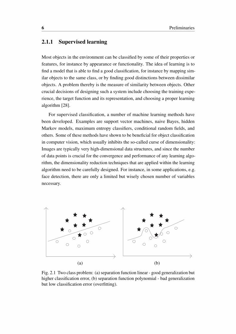
For supervised classification, a number of machine learning methods havebeen developed. Examples are support vector machines, naive Bayes, hiddenMarkov models, maximum entropy classifiers, conditional random fields, andothers. Some of these methods have shown to be beneficial for object classificationin computer vision, which usually inhibits the so-called curse of dimensionality:Images are typically very high-dimensional data structures, and since the numberof data points is crucial for the convergence and performance of any learning algo-rithm, the dimensionality reduction techniques that are applied within the learningalgorithm need to be carefully designed. For instance, in some applications, e.g.face detection, there are only a limited but wisely chosen number of variablesnecessary.

(a) (b)

Fig. 2.1 Two class problem: (a) separation function linear - good generalization buthigher classification error, (b) separation function polynomial - bad generalizationbut low classification error (overfitting).

2.1 Object classification 7

2.1.2 Overfitting

Overfitting [9] is an inherent aspect within every machine learning method. Itoccurs whenever the method learns the errors, e.g., measurement artefacts, in thetraining data rather than the actual underlying concept. It usually occurs whenthe model is too complex, i.e., having too many parameters relative to the giventraining data. An example is shown in Figure 2.1

In order to overcome overfitting, one of the approaches is to separate thetraining data set into data which is used for generating, or training, a model and intoa validation data set which is used to evaluate the trained model, containing mostlydata which has not been used for training the model. To provide enough evidenceagainst overfitting, the validation set should, if possible, be large enough to providea statistically significant sample of the instances to be learned. For example, atraining size of two thirds of all data and a validation size one third might beuseful [9]. For the interested reader, there exist other and more sophisticatedtraining and validation methods, e.g., cross-validation methods for situationswhere only few training data is available.

2.1.3 Ensemble learning

Ensemble classification methods provide a solution to overfitting. The termdefines learning methods that combine the output of multiple models, called baselearners, which might consist of different or the same types of learners. Theidea is that a diverse ensemble performs better than a single learner since everybase learner makes different errors and the errors average out when combined.The goal is therefore to create heterogeneous ensembles and strong ensembleswhich perform superior in comparison to homogeneous strong ensembles [14].Common ensemble classifiers are bagging, boosting and random forests [5] whichusually vary in the training of the individual base learners: In bagging, manybootstrap samples are drawn from a training data set with replacement in order toconstruct each tree independently from the others. Boosting, on the other hand,applies reiterative re-training by increasing the weight of previously incorrectlyclassified samples. Random forests, which will be analysed in the following, applybagging for random decision trees as base learners. They combine a randomizedselection of features with a locally optimized selection of discimiment featuresduring training.

8 Preliminaries

2.2 Random decision tree learning

This section describes random decision forests. After basic concepts to createdecision trees are introduced, the combination of multiple random decision treesinto a random forest is presented.

2.2.1 Decision tree learning

Historically, decision tree learning is a deterministic method for approximatingdiscrete-valued functions of attribute-value pairs that are to some degree robustto noisy data and capable of learning disjunctive expressions [28]. As a datastructure in computer science, the term tree describes an undirected or directed,fully connected, acyclic graph with only one root node. The here proclaimedtrees are directed graphs, or, more precisely, directed rooted trees. Nodes withoutoutgoing edges are called leaves, or terminal nodes, while nodes which includetests and are linked to more nodes, or to subtrees, are called non-terminal nodes.The root is the only node without an incoming link. In binary trees, each internalnode has two child nodes, which in practice often represent binary decisions. Eachleaf is usually assigned to one class representing the most frequent target value, orto a probability vector containing the probabilities of the target attribute havingcertain values. Instances are then classified by navigating from the root througha path, according to the test outcomes, until a leaf is reached. Learned trees canthen also be re-represented by a disjunction of conjunctions of constraints onthe attribute values of learned instances. Each path from the tree root to a leafcorresponds to a conjunction of attribute tests, and the tree itself is a disjunctionof these conjunctions [28]. In the case of numeric attributes, decision trees can beinterpreted as a set of hyperplanes, where each hyperplane is orthogonal to one ofthe axes.

An illustration of a decision tree for continuous feature values is presented inFigure 2.2. Internal nodes perform tests on features xi where i ∈ {1, ...,n}. Thenodes are described by the name of the feature and a threshold value θi on whichthe decision is based.

Since decision trees allow for the training data to contain missing attribute values,and since they may be interpreted quite intuitively as long as the tree depth is keptsmall enough, they have been applied to a variety of disciplines besides computervision, such as medical diagnosis, or credit risk analysis [28].

Many variants on how to train a decision tree exist, however, most of them arebased on a core algorithm that employs a top-down, greedy search through the

2.2 Random decision tree learning 9

Feature x 1

Feature x 2

Feature x 3

Class 3 Class 1 Class 2 Class 1

x < x >= θ

x < θ x >= x >= θx <

1

2 3θ

θ

θ

θ

θ

θ

1 1 1 1

2 2 2 2 3 3 3 3

Fig. 2.2 A decision tree representing a 3-class problem with 3 features (x1, x2,x3).

space of possible decision trees. A popular algorithm is ID3 [32] and C4.5 [33] asone of its extensions. The idea of ID3 is to select from all n features the one whichbest separates the training examples according to their target classification [28]. Adecision that makes further descending nodes as pure as possible [17], leadingto leaf nodes that distinguish the classes well, is preferred. Purity means thatindividuals which can be assigned to a certain node belong to the same class.

The entropy impurity of a node is an important measure and defined in Equation(2.1) for a two-class problem, where S is a collection of positive (⃝) and negative(⋆) training examples of some target concept. p⃝ is the ratio between individualsclassified as ⃝ and the number of all individuals, similarly for p⋆.

Entropy(S) =−p⋆ log2 p⋆− p⃝ log2 p⃝ (2.1)

This definition can be extended to a multi-class problem [9], see Equation (2.2):

Entropy(S) =−∑j

p(ω j) log2 p(ω j) (2.2)

where j ∈ {1..N}, N is the number of classes, and p(ω j) is the fraction oftraining data at node S that are in the category ω j. The entropy reaches zero whenall training examples are in the same category and reaches its maximum, e.g.,when all training data is equally distributed over the available classes.

The Gini impurity, given in Equation (2.3) is a similar measure. In contrastto entropy, all values of the Gini impurity lie in the interval of [0,1). It reaches

10 Preliminaries

its minimum of zero when all examples in a node fall into a single class and itsmaximum when the examples are equally distributed over the classes.

Gini(S) = 1−∑j

p(ω j)2 (2.3)

In the algorithm realization, the entropy-related measures are often used to calcu-late an information gain to be maximized at each node [28], see Equation (2.4).Basically, ID3 chooses the next feature to conduct a test in a node based on theinformation gain associated with the attributes.

Gain(S,A) = Entropy(S)− ∑v∈Values(A)

|Sv||S|

Entropy(Sv) (2.4)

Since the test that maximizes this information gain is selected at each node duringdecision tree learning, the algorithms belong to the family of greedy algorithmswhich perform locally optimal decisions.

According to Breiman [4], tree complexity affects a tree’s accuracy. The treecomplexity is controlled by the stopping criteria and the pruning decisions thatare applied during and after tree induction. The task of automatically constructingoptimal trees is considered an NP-hard problem. Practical issues within treelearning algorithms include determining the maximum depth to grow the decisiontree, as well as choosing an appropriate attribute selection measure to account forwhether a data split is statistically significant. Some of the most common stoppingcriteria include:

• All instances in the training set belong to the same class.

• The maximum tree depth has been reached.

• The number of datapoints in the terminal node would be smaller than theminimum number of datapoints for parent nodes.

• If the nodes were split, the number of datapoints in one or more child nodeswould be less than the minimal number of datapoints allowed within childnodes.

All these parameters have an influence on precision and on computational effi-ciency. The ID3 algorithm, for instance, grows each branch of the tree as deeplyas necessary to perfectly classify the training data. Although this strategy may

2.2 Random decision tree learning 11

be reasonable, it might lead to difficulties if the training data contains noise, asdiscussed in Section 2.1.2. In many real-world scenarios, the training data maynot be suitable to create representative decision rules.

Related to that is the idea to grow the full tree, and post-prune it later, as in theC4.5 algorithm [33]. Pruning a decision tree at a certain internal node involvesremoving the subtree at that node, turning it into a leaf node, and assigning it to themost common classification of the training examples in the subtree [34]. Anotherapproach are random decision trees that are usually the base classifiers in randomdecision forests, which will be presented in the next section.

Sample datausing bootstrap draws

Train datadata set to growthe single trees

Out-of-bag (OOB)data to estimate the

error of the gown tree

Feature selectionrandom selectionof feature subset

Grow treesplit data using

the best predictor

Estimate OOB errorby appling the treeto the OOB data

Random Forestas a collection of all trees

repeatuntilcriteriafor stopgrowing treeis fulfilled

repeatuntilspecifiednumberof trees isobtained

Fig. 2.3 Random forest training - algorithmic overview [2]

2.2.2 Random decision forests

In contrast to the algorithms of the ID3 family which optimize the tree structure byconsidering all possible features, random decision trees use a randomly selectedsubset of features. In addition, to reduce the variance of the classification estimate,several trees are trained on randomly sampled subsets of the data [5]. Therefore,

12 Preliminaries

in order to obtain less correlated classifiers, it is useful to chose both the datasubset and the feature subset randomly. An overview of the training procedure isillustrated in Figure 2.3. Single trees in a random forest when grown very deeptend to overfit the data since they learn more complex models, and therefore havea low bias, but a very high variance. By bootstrapping, the variance between treesis decreased.

Training more than a single random tree eventually leads to a random forest, anexample is shown in Figure 2.4. The overall system classification answer is thendone by the voting of the different decision trees on the test data, e.g. by averageor majority voting. Combining many diverse trees produces smooth decisionboundaries [6] [31].

...

x

+

y

Fig. 2.4 Schematic view of a decision forest, active nodes involved during classifi-cation depicted in red. Feature vector x, class label y, the combined average voteis denoted by the plus symbol.

In order to grow a random forest, the user is required to specify many inputparameters, such as the number of trees to grow, the number of features usedto split each node, the test selection criterion, as well as some stopping criteriasuch as the maximum depth of a tree and the maximum number of samples ina node. Decisions that lead to simple, compact trees with few nodes might bepreferred and are linked to Occam’s razor, which states that the simplest modelshould explain the data [9].

As described in this section, random forests posess many advantageous proper-ties. They are insensitive to noise in the training data, do not require pruning, andtheir error is measured automatically with out-of-bag data. Besides, there existseveral open-source frameworks for random forests [30]. A limitation is that their

2.3 Genetic algorithms 13

parameters must be set manually, and that their overall strength is dependent onthe strength of the individual trees and their correlation.

2.3 Genetic algorithms

Genetic algorithms refer to a family of algorithms from evolutionary computationand are used to search optimal parameters to a problem set. They are inspired bythe evolution of biologic populations, assuming that individuals or whole speciesreproduce according to their chance of survival or strength. Some introductionscan be found in [38] or [1]. As excellently discussed in [28], those individuals thatare able to adapt to their changing environment, i.e., that inherit an ability to learnby themselves, might be more competitive in contrast to those who cannot learn.

Apart from early artificial intelligence problems such as logic, genetic al-gorithms can be applied to problems handling large data such as web mining,computer vision and natural language processing. Since genetic algorithms maybe trained and executed in parallel, and take advantage of the decreasing cost ofcomputer hardware, they recently find applications in real-world scenarios, e.g.learning manipulation rules for robot control from visual input [27], in naturallanguage processing for part-of-speech tagging [25], or optimizing the learning pa-rameters for artificial neural networks [43]. Genetic algorithms are often describedas a global search method using no gradient information. Similar methods aregradient descent, stochastic hill-climbing and simulated annealing which mightwork within similar problem domains.

Unlike many algorithms in computer science which describe and solve a tasktop-down or bottom-up, i.e., from general to specific or from specific to general,genetic algorithms generate solution sets by repeatedly selecting and modifyingparts of the best known solutions found so far [28] [9] and thereby make relativelyfew problem assumptions. In contrast, several individual solutions are created toform a population. Each individual solution may vary from the other, which makesit possible to rank or score their performance or fitness. If the task is classification,the fitness function usually includes the classification accuracy over some providedtraining examples. Of course, there are no restrictions and other criteria can beused and combined in the fitness function.

This chapter introduces a basic version of a genetic algorithm, states importantproperties and design decisions, and finally presents some algorithmic extensionsthat might be interesting research opportunities for the experiments in this work.

14 Preliminaries

2.3.1 Genetic operations

Initialpopulation

Evaluation

Selection

Crossover

Mutation

New pop-ulation

Fig. 2.5 Basic steps of a genetic algorithm

A genetic algorithm employs stochastic variations which depend on the funda-mental representation of each individual solution. As found in the literature, therepresentations commonly utilized are binary strings, but since these so-calledchromosomes can be mapped arbitrarily to the feature domain, the possible rep-resentations are unlimited and may range from symbols of an alphabet overreal-valued numbers to any particular data types.

The usual genetic operations are presented in Figure 2.5. The single steps willbe described in the following.

2.3.1.1 Initial population

Before applying any of the genetic operands, an initial population needs to begenerated. Usually, the number of individuals to form a population is set to aconstant number and stays constant for each generation. The first population mightbe initialized randomly. However, alternative initilizations are possible such asextended random initialization in which each member of the initial population ischosen as the best of a number of randomly chosen individuals, also known asknowledge-based initialization.

2.3 Genetic algorithms 15

2.3.1.2 Fitness evaluation

Fitness evaluation of an individual describes an individuals’ strength or rankin comparison to the other individuals in the population. For example, if thelearning task is the problem of approximating an unknown model giving trainingexamples of its input and output, then fitness may be defined as the accuracy ofthe hypothesis over its training data. One example is a monotonic function ofthe accuracy on the data set, and possibly an additional penalty term to avoidoverfitting [9]. However, fitness may as well depend on multiple goals. Formulti-objective optimization problems for instance, there exist other techniquesexplained in [1] such as aggregating them by weights, measure their differencesfrom predefined goals for each objective, or finding pareto strategies. In addition,there exist attempts to incorporate the ancestors’ or siblings’ influence into thefitness of an individual, i.e., an individual is not considered as an independententity but is influenced by its surroundings. Consequently, the offspring maye.g. incorporate knowledge from siblings or parents. After fitness is evaluated, anew generation will be created by the following genetic operations.

(a)

(b)

Fig. 2.6 Different sampling strategies, 10 samples are generated based on thefitness of 10 individuals: (a) Low-variance sampling; (b) 2 possible outcomes(upper or lower arrows) for roulette-wheel sampling.

The fitness function might depend on multiple goals to be optimized apart fromclassification accuracy, such as the model complexity or contribution to the wholepopulation. If the tree provides a contribution to the strength of the whole ensemble,and adds to its diversity, it should be selected to bring offspring into the nextgeneration.

16 Preliminaries

parents (generation k)

offspring (generation k+1)

replication crossover mutation

Fig. 2.7 Basic operations of a genetic algorithm, above the line are one or twomembers of the old generation, below the new ones. The example representationis a binary string. Simplified version of the graphics presented in [9].

2.3.1.3 Selection

To select the candidates from the current population to create offspring, selectionis usually done proportionally to the fitness. This can be done by low-variance orby stochastic sampling, e.g., by roulette wheel selection. As depicted in Fig. 2.6,the outcome of roulette-wheel sampling is much more random (Fig. 2.6 (b) )than for low-variance sampling (Fig. 2.6 (a) ). Especially for a low number ofindividuals, to keep the sampling process less random and the population morestable, low-variance sampling may be the preferred selection method. Therealso exist forms of selection to parallelize the selection process. In tournamentselection, two hypotheses are first chosen at random from the population, and witha certain probability the more fit or the less fit of these two is finally selected. Incontrast to roulette wheel selection, this strategy often leads to a more diversepopulation.

After selection, the subsequent genetic operations are illustrated in Figure 2.7.Crossover and mutation yield the next generation, and both operations can lead tolarge changes among members of the population. These changes can be useful toget out of local optima, making local optima sometimes easier to deal with than inother methods such as gradient descend.

2.3 Genetic algorithms 17

2.3.1.4 Crossover

Crossover recombines two parent chromosomes to produce a new chromosomethat shares features from both parents [1]. There are variants including point-crossovers or uniform crossover. The conditions under which crossover occursmay be random or depend on special critera such as if a certain distance, hammingdistance in case of string comparisons between two parent individuals, is above acertain threshold. In biologic populations, this strategy might be linked to incestprotection.

2.3.1.5 Mutation

Mutation indicates that some elements of the DNA are slightly changed which maybe caused by errors in copying genes from parents. For instance, the characters ofa DNA, i.e., the alleles from a current chromosome, might change at random witha small probability, as described in [1]. A possible technique is called adaptivemutation, whereby the probability to perform a mutation increases with an increaseof the genetic homogeneity in the total population [42]. Other methods tend tokeep the population stable once a certain fitness has been reached. Therefore, anoption is to start the genetic training process with a high mutation rate, and then tolet the mutation rate decrease, e.g., exponentially with every mutation step. Thechoice of certain mutation methods depends on the problem.

2.3.2 Known problems

In general, genetic algorithms cannot guarantee the improvement of a population,neither can they guarantee the convergence to a global fitness optimum. However,copying the best individuals to the next generation assures that the population willnot worsen (without mutation and recombination), which is a phenomenon referredto as elitism. In addition, genetic algorithms are non-deterministic, meaning thatdifferent runs lead to different results depending on the seed of the random numbergenerator. However, in case the problem does not have one single best solution,i.e., various solutions close to a desired optimum can be accepted, they are usefuland often work better than traditional methods [16]. Since each individual in agenetic algorithm represents a hypothesis to a given problem, genetic algorithmsare sometimes also interpreted as multi-hypotheses approaches. In comparison tosingle-hypothesis approaches, the probability of getting stuck in a local optimumcan be reduced. On the other hand, genetic algorithms can get stuck in local optimaas well. The term crowding describes the phenomena during multiple episodes

18 Preliminaries

that if a certain individual has a very high fitness compared to the other individualsin the population, under circumstances, an undesired rather large amount of directand similar copies of this individual may survive into next generations. As adisadvantage, having too many alike individuals may then impact the result of thepopulation as well.

2.3.3 Design choices

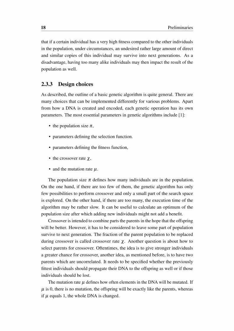
As described, the outline of a basic genetic algorithm is quite general. There aremany choices that can be implemented differently for various problems. Apartfrom how a DNA is created and encoded, each genetic operation has its ownparameters. The most essential parameters in genetic algorithms include [1]:

• the population size π ,

• parameters defining the selection function.

• parameters defining the fitness function,

• the crossover rate χ ,

• and the mutation rate µ .

The population size π defines how many individuals are in the population.On the one hand, if there are too few of them, the genetic algorithm has onlyfew possibilities to perform crossover and only a small part of the search spaceis explored. On the other hand, if there are too many, the execution time of thealgorithm may be rather slow. It can be useful to calculate an optimum of thepopulation size after which adding new individuals might not add a benefit.

Crossover is intended to combine parts the parents in the hope that the offspringwill be better. However, it has to be considered to leave some part of populationsurvive to next generation. The fraction of the parent population to be replacedduring crossover is called crossover rate χ . Another question is about how toselect parents for crossover. Oftentimes, the idea is to give stronger individualsa greater chance for crossover, another idea, as mentioned before, is to have twoparents which are uncorrelated. It needs to be specified whether the previouslyfittest individuals should propagate their DNA to the offspring as well or if thoseindividuals should be lost.

The mutation rate µ defines how often elements in the DNA will be mutated. Ifµ is 0, there is no mutation, the offspring will be exactly like the parents, whereasif µ equals 1, the whole DNA is changed.

2.3 Genetic algorithms 19

After discussing the most essential components of a genetic algorithm, thenext chapters will focus on the application of a genetic algorithm to generatingrandom forests for a computer vision problem.

Chapter 3

Implementation

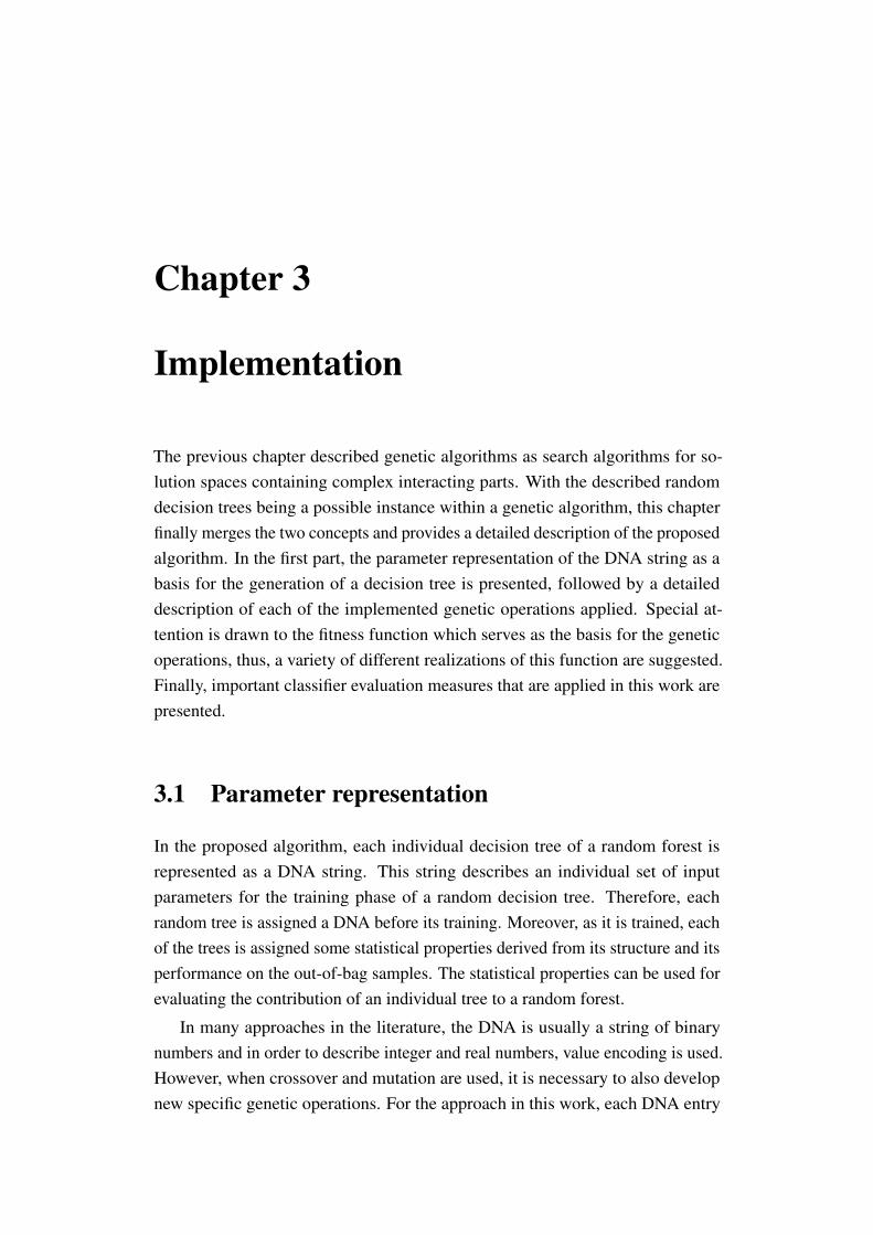
The previous chapter described genetic algorithms as search algorithms for so-lution spaces containing complex interacting parts. With the described randomdecision trees being a possible instance within a genetic algorithm, this chapterfinally merges the two concepts and provides a detailed description of the proposedalgorithm. In the first part, the parameter representation of the DNA string as abasis for the generation of a decision tree is presented, followed by a detaileddescription of each of the implemented genetic operations applied. Special at-tention is drawn to the fitness function which serves as the basis for the geneticoperations, thus, a variety of different realizations of this function are suggested.Finally, important classifier evaluation measures that are applied in this work arepresented.

3.1 Parameter representation

In the proposed algorithm, each individual decision tree of a random forest isrepresented as a DNA string. This string describes an individual set of inputparameters for the training phase of a random decision tree. Therefore, eachrandom tree is assigned a DNA before its training. Moreover, as it is trained, eachof the trees is assigned some statistical properties derived from its structure and itsperformance on the out-of-bag samples. The statistical properties can be used forevaluating the contribution of an individual tree to a random forest.

In many approaches in the literature, the DNA is usually a string of binarynumbers and in order to describe integer and real numbers, value encoding is used.However, when crossover and mutation are used, it is necessary to also developnew specific genetic operations. For the approach in this work, each DNA entry

22 Implementation

contains an integer value or a vector of continuous values. The DNA has beenconstructed to include the parameters given in Table 3.1.

Table 3.1 The parameters of the DNA of a random decision tree

Parameter name DescriptionMaximum height The maximum height of a tree; at maximum tree

height, no internal nodes are produced anymore.Minimum datapoints The minimum number of datapoints needed to perform

a split in a node, i.e., to create an internal node.Maximum datapoints The maximum number of datapoints needed to per-

form a split in a node, i.e., to create an internal node.Number of tests The number of tests to generate randomly within each

internal node from which the best one is chosen ac-cording to the specified score and split criteria.

Scoring function The scoring function used, may be either label-dependent or label-indepedent.

Split Point Selection The split point selection method, may be either label-independent or label-dependent.

Feature probability A probability vector for every feature category.Test probability A probability vector for every test category.

The parameter’s influence of the performance in a random forest has been investi-gated by Hänsch [15], whose framework has been applied and extended in thiswork. For an analysis on the scoring and split functions that were utilized, thereader is referred to [15].

3.2 Genetic operations

When optimizing a function, the space of all possible solutions is called a searchspace, or state space [34]. Each point in the search space represents one possiblesolution, and each possible solution can be assigned a value, or fitness, for theproblem. The optimization of a solution is equal to finding an extreme (minimumor maximum) in the search space. The search space might be well-known. Usually,however, only few points in it are know and more points need to be continuouslygenerated in the process of finding an optimum. A further problem is that the

3.2 Genetic operations 23

search space may be quite complicated in terms of multiple local optima, makingit difficult to estimate a good initial parameters set. This is a common problemwith other search methods such as hill climbing and simulated annealing.

3.2.1 Fitness evaluation

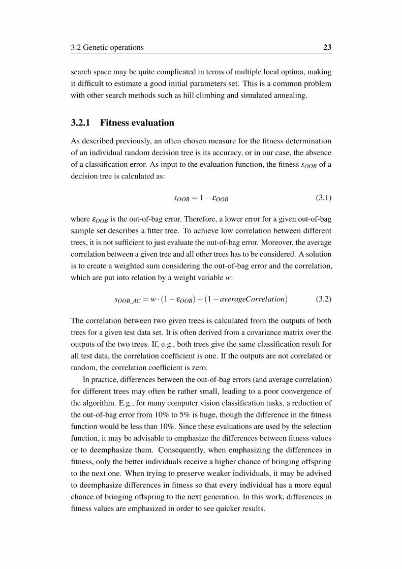
As described previously, an often chosen measure for the fitness determinationof an individual random decision tree is its accuracy, or in our case, the absenceof a classification error. As input to the evaluation function, the fitness sOOB of adecision tree is calculated as:

sOOB = 1− εOOB (3.1)

where εOOB is the out-of-bag error. Therefore, a lower error for a given out-of-bagsample set describes a fitter tree. To achieve low correlation between differenttrees, it is not sufficient to just evaluate the out-of-bag error. Moreover, the averagecorrelation between a given tree and all other trees has to be considered. A solutionis to create a weighted sum considering the out-of-bag error and the correlation,which are put into relation by a weight variable w:

sOOB_AC = w · (1− εOOB)+(1−averageCorrelation) (3.2)

The correlation between two given trees is calculated from the outputs of bothtrees for a given test data set. It is often derived from a covariance matrix over theoutputs of the two trees. If, e.g., both trees give the same classification result forall test data, the correlation coefficient is one. If the outputs are not correlated orrandom, the correlation coefficient is zero.

In practice, differences between the out-of-bag errors (and average correlation)for different trees may often be rather small, leading to a poor convergence ofthe algorithm. E.g., for many computer vision classification tasks, a reduction ofthe out-of-bag error from 10% to 5% is huge, though the difference in the fitnessfunction would be less than 10%. Since these evaluations are used by the selectionfunction, it may be advisable to emphasize the differences between fitness valuesor to deemphasize them. Consequently, when emphasizing the differences infitness, only the better individuals receive a higher chance of bringing offspringto the next one. When trying to preserve weaker individuals, it may be advisedto deemphasize differences in fitness so that every individual has a more equalchance of bringing offspring to the next generation. In this work, differences infitness values are emphasized in order to see quicker results.

24 Implementation

The fitness value s has been scaled by the help of a transfer function h. Thenew fitness value s is used to emphasize the differences, that, given an input fitness,creates a scaled version of the fitness, as calculated in Equation (3.3). For every 5percent that s increases, h(s) = s doubles:

s = h(s) = 21

0.05 ·s = 220.0·s (3.3)

sOOB = 220.0·sOOB (3.4)

sOOB_AC = 220.0·sOOB_AC (3.5)

where sOOB is the scaled fitness value for a tree considering both its out-of-bagerror and sOOB_AC is the scaled fitness value for a tree considering its out-of-bagerror and its average correlation with the other trees.

3.2.2 Selection

Selection has been realized as low-variance sampling as described in 2.6, wherebythe fitness values for all trees are stored in a vector and then low-variance samplingchooses as many individuals as desired. For example, if there are 20 trees, onemight want to select 15 trees by low-variance sampling, and the remaining fivetrees by another selection procedure.

Another common strategy is to select the best individual according to their rankand to guarantee for them to create offspring for the next generation. However, thiswork tries to be as probabilistic as possible. In ranking, the differences betweenthe first and the second best individual, for instance, is not really well represented.Doing a probabilistic sampling seems the better choice.

Instead of using this procedure to select all the individuals in a population,another variant is to replace the worst individuals by randomly creating newindividuals, which are constructed similarly to the procedure to create the initialpopulation. One criteria to do so may occur if the entropy over all individuals’fitnesses is very low (all trees have similar fitness values, i.e., score similarly),or if the overall correlation value is above a certain threshold. Then it might bebeneficial to replace some of the individuals by newly created ones to avoid gettingstuck in a local maximum. On the other hand, if the individual trees convergeinto a region where all individuals receive a high fitness, one may not desire tocreate many new randomly initialized individuals as a form of adding noise to theprevious distribution of trees because it can degrade the fitness of the population.

3.2 Genetic operations 25

Table 3.2 Select a tree with a high fitness

Tree Nr. 1 2 3 4 5 6 7 8 9 10Error 0.28 0.32 0.34 0.29 0.37 0.31 0.28 0.21 0.26 0.37Strength 0.71 0.67 0.65 0.70 0.62 0.68 0.71 0.78 0.73 0.62Norm.strength 0.10 0.09 0.09 0.10 0.09 0.09 0.10 0.11 0.10 0.09Exp.in 10−2 207 110 87 173 55 126 202 504 266 56Norm.Exp. 0.11 0.06 0.04 0.09 0.03 0.07 0.11 0.28 0.14 0.03

3.2.3 Anti-correlation-based selection

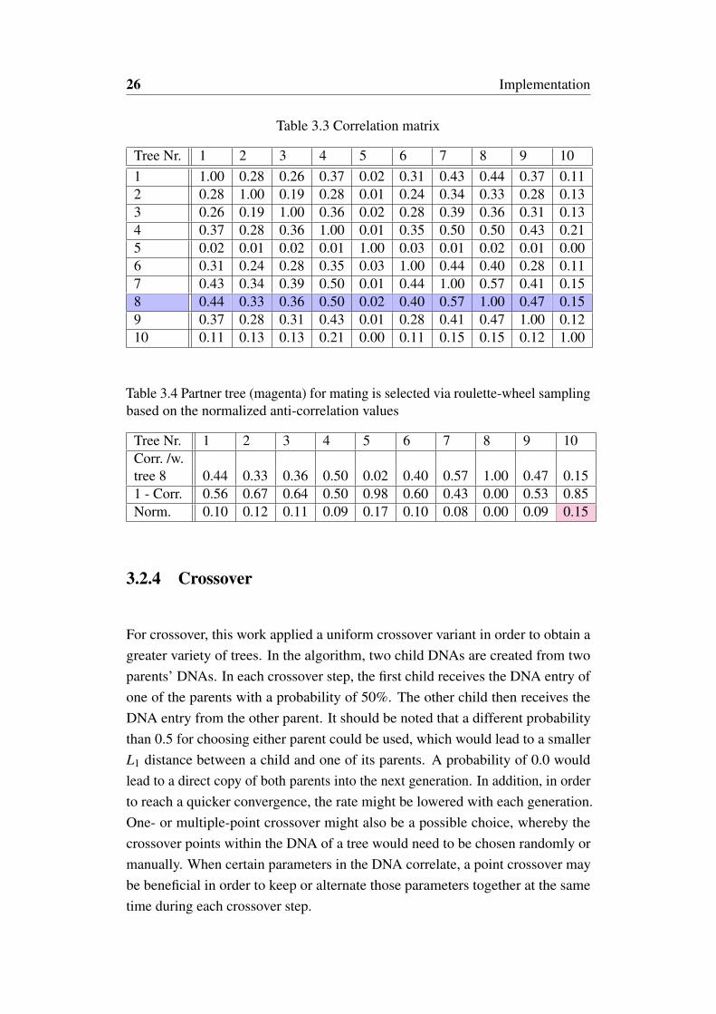
One method to create less correlated trees that has been implemented in this workis to select two partners who are allowed to copy their DNAs into the offspring.The idea is that one of the partners should be strong, and its partner candidateshould be uncorrelated to the first one. The first candidate is chosen by a samplingprocedure based on the scaled and normalized out-of-bag error of all individuals,as illustrated in Table 3.2. The term Error defines for each of the 10 trees theroot-mean-squared (RMS) error, explained in Section 3.6, which is calculatedfrom the ration between misclassified examples and all examples within the out-of-bag data during the training of a tree, illustrated in Figure 2.3. After evaluatingthe performance of a tree by 1−Error, the strengths of all trees are normalized.Applying the discussed exponential function from Equation 3.3 leads to a scaledstrength for each tree, in which the differences between the fitness values areemphasized. This scaled strength is furthermore normalized, and serves as afitness value for the sampling of the first individual. In the example in Table 3.2,tree 8 has been selected.

The second individual is chosen by a different method which is illustratedin Table 3.4. Based on the correlation matrix between all trees, cf. Table 3.3,for the tree that has been sampled in the first method (in the example tree 8), apartner tree with a low correlation is desired. Therefore, the corresponding rowof the correlation matrix is extracted and the amount of each correlation value issubtracted from a vector of ones. After a normalization of the resulting vector,a roulette-wheel sampling takes place in order to obtain a partner tree. In theexample, tree 10 has been selected.

26 Implementation

Table 3.3 Correlation matrix

Tree Nr. 1 2 3 4 5 6 7 8 9 101 1.00 0.28 0.26 0.37 0.02 0.31 0.43 0.44 0.37 0.112 0.28 1.00 0.19 0.28 0.01 0.24 0.34 0.33 0.28 0.133 0.26 0.19 1.00 0.36 0.02 0.28 0.39 0.36 0.31 0.134 0.37 0.28 0.36 1.00 0.01 0.35 0.50 0.50 0.43 0.215 0.02 0.01 0.02 0.01 1.00 0.03 0.01 0.02 0.01 0.006 0.31 0.24 0.28 0.35 0.03 1.00 0.44 0.40 0.28 0.117 0.43 0.34 0.39 0.50 0.01 0.44 1.00 0.57 0.41 0.158 0.44 0.33 0.36 0.50 0.02 0.40 0.57 1.00 0.47 0.159 0.37 0.28 0.31 0.43 0.01 0.28 0.41 0.47 1.00 0.1210 0.11 0.13 0.13 0.21 0.00 0.11 0.15 0.15 0.12 1.00

Table 3.4 Partner tree (magenta) for mating is selected via roulette-wheel samplingbased on the normalized anti-correlation values

Tree Nr. 1 2 3 4 5 6 7 8 9 10Corr. /w.tree 8 0.44 0.33 0.36 0.50 0.02 0.40 0.57 1.00 0.47 0.151 - Corr. 0.56 0.67 0.64 0.50 0.98 0.60 0.43 0.00 0.53 0.85Norm. 0.10 0.12 0.11 0.09 0.17 0.10 0.08 0.00 0.09 0.15

3.2.4 Crossover

For crossover, this work applied a uniform crossover variant in order to obtain agreater variety of trees. In the algorithm, two child DNAs are created from twoparents’ DNAs. In each crossover step, the first child receives the DNA entry ofone of the parents with a probability of 50%. The other child then receives theDNA entry from the other parent. It should be noted that a different probabilitythan 0.5 for choosing either parent could be used, which would lead to a smallerL1 distance between a child and one of its parents. A probability of 0.0 wouldlead to a direct copy of both parents into the next generation. In addition, in orderto reach a quicker convergence, the rate might be lowered with each generation.One- or multiple-point crossover might also be a possible choice, whereby thecrossover points within the DNA of a tree would need to be chosen randomly ormanually. When certain parameters in the DNA correlate, a point crossover maybe beneficial in order to keep or alternate those parameters together at the sametime during each crossover step.

3.3 Classifier evaluation 27

3.2.5 Mutation

Similarly to selection and to fitness evaluation, there exist multiple variants formutation. Compared to a gradient descent algorithm, where a parameter vector isoptimized during subsequent training iterations by a certain distance towards thedirection of the steepest gradient, the parameter vectors in GAs are altered andevaluated for different directions in the parameter space. Unlike in gradient descentin which the step distance usually decreases over time, in this work, the mutationrate stays constant. In this implementation, the tree height is altered within aninteger interval [−5,5] (without zero), the number chosen is uniform randomlydetermined for each mutation step for each individual tree. The minimum andmaximum split points have also been chosen to be mutated within an interval[−5,5] (without zero). The probability for a feature and test selection have beenchosen be be mutated by randomly recreating them by a Dirichlet distribution.

3.3 Classifier evaluation

To describe the performance of any learning system, the generalization error hasto be measured. In this work, multiple error measures are utilized to evaluate boththe whole forest and the individual trees by investigating their performance ontraining and on test data. There are several ways to measure the overall system’serror. One of them, which has been applied in the random forest framework of[15], is the Root-Mean-Squared (RMS) error which can be used on soft outputand provides a scalar to judge the system, and is presented in Equation (3.6)

ERMS =1Z·∑

i∑x,y

||yest − yre f ||2 (3.6)

where yest is a category-probability-vector that has been estimated and yre f

is the desired reference category distribution vector, (x,y) are pixels within allimages i of the current dataset for which reference data exists, and Z is the sum ofall pixels [15].

Another measure to calculate the performance of the ensemble of tree classi-fiers is the confusion matrix, which counts how many samples of one class areconsidered by the system to belong to another class within the predicted data.The confusion matrix of a strong classifier should contain probabilities close to1 only at its main diagonal and probabilities close to 0 at all other matrix entries.The basic layout of a confusion matrix is given in Table 3.5, from which the

28 Implementation

true positive rate (T PR), or hit rate, and the true negative rate (T NR), or correctrejection rate, in contrast to the false positive (FPR), or false alarm rate, and thefalse negative rate (FNR), or miss rate, are derived.

actu

alva

lue

Prediction outcome

p n total

p’TruePositive(TP)

FalseNegative(FN)

P’

n’FalsePositive(FP)

TrueNegative(TN)

N’

total P NTable 3.5 Confusion matrix for a two-class problem

T PR =T P

T P+FN=

T PP

(3.7)

FPR =FP

FP+T N=

FPN

(3.8)

T NR = 1−FPR =T NN

(3.9)

FNR = 1−T PR =FNP

(3.10)

Cross-validation is usually a key to finding optimal parameters. This is alreadydone during an OOB estimation of the generalization error. Since random forestsemploy an internal accuracy measure, it is not necessary to divide the referencedata into separate sets for training and validation. Instead, the test set accuracy isestimated by running out-of-bag (OOB) samples, which refer to a subset of thetraining data that was not included in the bootstrap for a particular tree by usingthat subset of samples at a tree [3] [5].

3.4 Summary 29

3.4 Summary

There exist many possible solutions for different operations of the genetic algo-rithm. Important implementation choices and issues have been described in thischapter. To evaluate their impact on the classification strength of the geneticrandomized trees system, a number of experiments have been performed. Theexperiments and the results will be presented in the next chapter.

Chapter 4

Experiments

This chapter provides a description and an evaluation of the experiments performed.It first describes the training and test data that was used in the experiments, aswell as the random forest framework which has been extended by a geneticalgorithm. This chapter concentrates on how different fitness functions, mutationrates, considerations of correlations and crossover functions contribute to theclassification accuracy and correlation of the generated forests. After an overviewof the conducted experiments, their results and a discussion are presented.

4.1 Description of the experiments

The goal of the experiments is to evaluate the different parts of the genetic opera-tions presented in Chapter 3. Therefore, the experiments will focus on the mutation,selection, scaled selection as a variant of selection, anti-correlation-based selectionas another variant, and on crossover. In order to evaluate the experiments, in eachgeneration within the genetic framework, this work is concerned with the forests’out-of-bag error, the the forest’s test error, and with the forest’s overall correlationvalue.

As described in the previous chapter, different versions of the genetic opera-tions exist and can be differently combined. Since it is impossible to consider allcombinations of design choices with separate experiments, the experiments wereconducted step by step focusing on each aspect of the genetic algorithm separately.

Table 4.1 gives an overview of the experiments that were conducted:

• Experiment 1: Preliminary experiment investiging the convergence of thetree length, starting at tree length 1, using different fitness functions sOOB

and sOOB as described in Section 3.2.1

32 Experiments

• Experiment 2: Initializing all parameters randomly, different mutation ratesµ , using different fitness functions sOOB and sOOB as described in Section3.2.1

• Experiment 3: Investigating the standard deviation of the out-of-bag errorfor different runs based on sOOB

• Experiment 4: Same is Experiment 3, but using an anti-correlation-basedselection for a partner individual for an individual based on sOOB and sOOB

as described in Section 3.2.3

• Experiment 5: Same as Experiment 2, but using a selection based on a linearcombination of the out-of-bag error and the average correlation, sOOB_AC asdescribed in Section 3.2.1

• Experiment 6: Same as Experiment 5, but including an anti-correlationbased crossover as described in Section 3.2.4

Table 4.1 Overview of the conducted experiments

Exp. nr. MutationsOOB

basedselection

sOOB

basedselection

Anti-correlation-

basedselection

sOOB_AC

basedselection

Anti-correlation-

basedcrossover

1 X X

2 X X X

3 X X

4 X X X X

5 X X

6 X X X

4.1 Description of the experiments 33

(a) (b) (c)

(d) (e) (f)

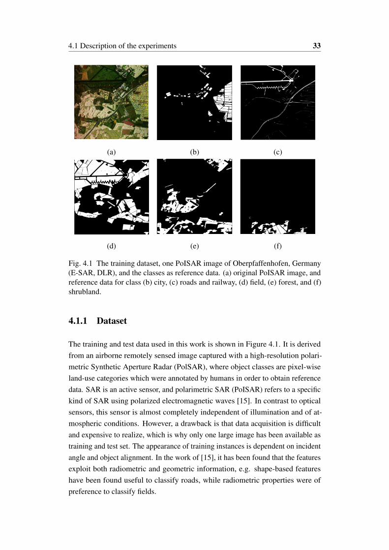
Fig. 4.1 The training dataset, one PoISAR image of Oberpfaffenhofen, Germany(E-SAR, DLR), and the classes as reference data. (a) original PoISAR image, andreference data for class (b) city, (c) roads and railway, (d) field, (e) forest, and (f)shrubland.

4.1.1 Dataset

The training and test data used in this work is shown in Figure 4.1. It is derivedfrom an airborne remotely sensed image captured with a high-resolution polari-metric Synthetic Aperture Radar (PolSAR), where object classes are pixel-wiseland-use categories which were annotated by humans in order to obtain referencedata. SAR is an active sensor, and polarimetric SAR (PoISAR) refers to a specifickind of SAR using polarized electromagnetic waves [15]. In contrast to opticalsensors, this sensor is almost completely independent of illumination and of at-mospheric conditions. However, a drawback is that data acquisition is difficultand expensive to realize, which is why only one large image has been available astraining and test set. The appearance of training instances is dependent on incidentangle and object alignment. In the work of [15], it has been found that the featuresexploit both radiometric and geometric information, e.g. shape-based featureshave been found useful to classify roads, while radiometric properties were ofpreference to classify fields.

34 Experiments

4.1.2 Framework

This work has been an extension of the projection-based random forest frameworkProB-RF by Hänsch [15] which works for image data using random spacialprojections, similar to Lepetit [23]. The random forest makes use of a large set ofgeneral low-feature operators capturing radiometric and textual properties usingsimple patch-based binary features inspired from the work by Lepetit [24] [23]who applied keypoint recognition using simple local patches centered at keypoints.The features are extracted from image patches, from which data points are selectedand projected in one dimension using multiple points or single points extractedfrom polarimetric, color, greyscale, or binary data. For the test function within thenodes of the trees in the random forest, a simple threshold operator is used.

4.1.3 System setup

The experiments have been performed on an Intel i7-4790 quadcore CPU with 16gigabytes of RAM, as an operation system served a 64-bit version of Ubuntu 14.4.The code of the genetic algorithm and the random forest has been written in C++.

4.1.4 Parameter setup

The parameters of the DNA within the first generation were initialized randomlywithin interval borders which are specified separately for each experiment. Unlessotherwise stated, the initial tree height was allowed to range from 1 to 10, andthe number of tests from 1 to 18. This work by default used a population sizeof 20 individuals, and runs experiments between 25 and 30 generations withthe different mutation rates, crossover rates, and fitness measures specified ineach experiment. Since both the random forest and the genetic algorithm exhibitrandomness, this work performed each experiment, whenever possible, multipletimes. In each run, the classification error and the correlation of each forestbased on the outcomes calculated from the out-of-bag estimates, as well as theclassification error calculated on a separate test set were recorded and plotted pergeneration.

4.2 Results and discussion

Experiment 1 The first and preliminary experiment was conducted to showwhether the strength of an ensemble of random decision trees improves if onlyselection with a subsequent mutation is applied over the course of multiple genetic

4.2 Results and discussion 35

selection based on sOOB selection based on sOOB

tree id

05

1015

2025 generation number

05

1015

2025

tree

heig

ht

0

5

10

15

20

25

30

tree id

05

1015

2025 generation number

05

1015

2025

tree

heig

ht

0

5

10

15

20

25

30

(a) (b)

tree id

05

1015

2025

generation number

05

1015

2025

out-of-bag error

0.00

0.05

0.10

0.15

0.20

0.25

0.30

0.35

0.40

tree id

05

1015

2025

generation number

05

1015

2025

out-of-bag error

0.00

0.05

0.10

0.15

0.20

0.25

0.30

0.35

0.40

(c) (d)

0 5 10 15 20 25

generation number0.10

0.15

0.20

0.25

0.30

0.35

erro

r

out-of-bag error test error

0 5 10 15 20 25

generation number0.10

0.15

0.20

0.25

0.30

0.35

erro

r

out-of-bag error test error

(e) (f)

Fig. 4.2 Experiment 1: Comparison of different fitness functions over 25 gen-erations. Left column: fitness wrt. out-of-bag error, cf. Eq. (3.1); right column:fitness wrt. exponentially transformed out-of-bag error, cf. Eq.(3.4). (a) and (b):Tree heights, (c) and (d): Out-of-bag error for each tree, (e) and (f): Out-of-bagand test error of the whole forest.

36 Experiments

generations. Therefore, in this first experiment, all 20 trees have been initializedwith a tree height of 1. The selection operation described in Section 3.2.2 was atfirst applied proportional to a single decision tree’s out-of-bag error, cf. Equation(3.1), and in a second run proportional to the exponential transformed fitness,cf. Equation (3.2). Sampling took place in a low-variance manner, cf. Figure 2.6,and mutation was applied to all DNA parameters as described in Chapter 3 witha mutation rate of µ = 1.0. The results of Experiment 1 are shown in Fig. 4.2.As expected, the application of selection and mutation lead to an increase in theaverage tree heights, resulting in an increase of the forest’s overall accuracy on theout-of-bag and the test data. In addition, applying the exponentially scaled fitnessfunction in comparison to the normal fitness produced higher and more accuratetrees in earlier generations.

Experiment 2 The next experiment was performed to investigate the influenceof the exponential scaling function to the convergence of the out-of-bag error,training error and the correlation of each forest in each generation. It was carriedout over 30 generations, with a population size of 20 trees. The initial population ofrandom decision trees was initialized in random intervals, whereby the maximumtree height has been randomly chosen to be between 1 and 10, the number of testswas randomly chosen between 1 and 10, the minimum and maximum number ofelements for a split have been chosen to range from 1 to 30, and the scoring andtest function have been randomly chosen, while the test and feature probabilityvectors were generated by Dirichlet sampling. Different mutation rates µ ∈{0.0,0.25,0.5} were investigated. The fitness was either based on the out-of-bagerror proportional function sOOB, or to a the exponential fitness function sOOB.

The results are shown in Figure 4.3. As can be seen in (a), applying selectionbased on only fitness values lead to almost no improvement in all of the threeconducted runs. As can be seen, the graphs for the out-of-bag error, training error,and correlation fluctuate to a greater extend when larger mutation rates are chosen.In contrast to this finding, in the results depicted in (b), in which an exponentialevaluation is applied to all trees before selection take place, leads to a visibleoptimization in the form of a decrease in both out-of-bag and test error. However,as can be seen when comparing the errors with the correlation value of the forests,per generation, both behave contrarily – each increase of the correlation lead to adecrease in the error and vice versa.

Experiment 3 In order to investigate the fluctuations between experiments,three runs have been started with a mutation rate of 0.1 and the other parameters

4.2 Results and discussion 37

5 10 15 20 25 300.170.180.190.200.210.220.230.240.25

out-o

f-bag

erro

r

5 10 15 20 25 300.200.210.220.230.240.250.260.270.28

test

erro

r

5 10 15 20 25 30generation number

0.30

0.35

0.40

0.45

0.50

0.55

corre

latio

n

µ=0.0 µ=0.25 µ=0.5

(a)

5 10 15 20 25 300.120.140.160.180.200.220.24

out-o

f-bag

erro

r

5 10 15 20 25 300.120.140.160.180.200.220.240.260.28

test

erro

r

5 10 15 20 25 30generation number

0.40

0.45

0.50

0.55

0.60

0.65

corre

latio

n

µ=0.0 µ=0.25 µ=0.5

(b)

Fig. 4.3 Experiment 2: Different mutation rates and uses of the scale function. (a)sOOB based selection, (b) sOOB based selection.

as described in Experiment 2. The resulting out-of-bag errors are depicted inFigure 4.4. As can be seen, the fluctuations are only small with an approximatestandard deviation of 0.02.

38 Experiments

0 5 10 15 20 25 30generation number

0.12

0.14

0.16

0.18

0.20

0.22

0.24

0.26

out-o

f-bag

erro

r

Fig. 4.4 Experiment 3: Mean and standard deviation of the forests’ out-of-bag erros during 30 generations, with a mutation rate of 0.1 and an otherwiseinitialization exactly as in Experiment 2.

5 10 15 20 25 300.100.120.140.160.180.200.220.240.26

out-o

f-bag

erro

r

5 10 15 20 25 300.10

0.15

0.20

0.25

test

erro

r

5 10 15 20 25 30generation number

0.350.400.450.500.550.600.65

corre

latio

n

µ=0.0 µ=0.25 µ=0.5

Fig. 4.5 Experiment 4: Different mutation rates when using selection of a fit anda low correlated individual as described in Section 3.2.3.

Experiment 4 The next experiment tried to evaluate a possible improvement byapplying a selection that is based on two pairs of individuals where one is chosenfrom the fittest individuals and its partner as an individual with a low correlation to

4.2 Results and discussion 39

it, as described in detail in Section 3.2.3. The results are shown in Figure 4.5. Ascan be seen, the fluctuations have been larger, and only a small improvement wasfound since the correlation increased slightly slower. The problem of crowding,described in Section 2.3.2, occured when the mutation rate µ was set to zero:After the tenth generation, almost all of the trees are so similar that the followinggenetic operations have no effect, leading to nearly constant errors and correlationvalues.

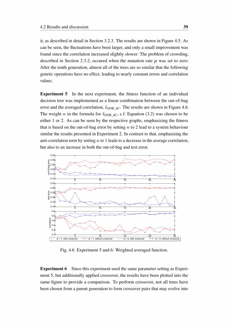
Experiment 5 In the next experiment, the fitness function of an individualdecision tree was implemented as a linear combination between the out-of-bagerror and the averaged correlation, sOOB_AC. The results are shown in Figure 4.6.The weight w in the formula for sOOB_AC, c.f. Equation (3.2) was chosen to beeither 1 or 2. As can be seen by the respective graphs, emphasizing the fitnessthat is based on the out-of-bag error by setting w to 2 lead to a system behavioursimilar the results presented in Experiment 2. In contrast to that, emphasizing theanti-correlation term by setting w to 1 leads to a decrease in the average correlation,but also to an increase in both the out-of-bag and test error.

5 10 15 20 250.10

0.15

0.20

0.25

0.30

0.35

out-o

f-bag

erro

r

5 10 15 20 250.10

0.15

0.20

0.25

0.30

0.35

test

erro

r

5 10 15 20 25generation number

0.1

0.2

0.3

0.4

0.5

0.6

corre

latio

n

w = 1, with crossover w = 1, without crossover w = 2, with crossover w = 2, without crossover

Fig. 4.6 Experiment 5 and 6: Weighted averaged function.

Experiment 6 Since this experiment used the same parameter setting as Experi-ment 5, but additionally applied crossover, the results have been plotted into thesame figure to provide a comparison. To perform crossover, not all trees havebeen chosen from a parent generation to form crossover pairs that may evolve into

40 Experiments

the next generation, but a subset of 10 trees. As can be seen in Figure 4.6, theresults are similar to the ones obtained when not using crossover, and the overalldevelopment of the graphs appear to be within the limits of random fluctuation.

4.3 Summary

The experiments showed that the genetic algorithm is able to improve the classifica-tion accuracy of the random forest. However, the contribution to this convergencewas strong for some operations, but weaker for others. Choosing the exponentialfitness function over the normal fitness function lead to a much faster conver-gence. The mutation rate had a strong impact on both convergence and stability ofthe genetic algorithm. Both methods to decrease correlation between trees, i.e.,anti-correlation based selection, and selection based on a linear combination ofout-of-bag error and average correlation, had unfortunately either no effect on theoverall correlation, or the lower correlation was linked to a higher out-of-bag error.The effect of crossover was non-significant. Future work needs to investigate otherfitness functions and methods to create less correlated ensembles.

Chapter 5

Conclusion

5.1 Summary

Finding the right parameter set for random forests, as for other machine learningapproaches is a non-trivial task and usually requires a certain amount of experiencefrom the human expert. This work showed that the application of a geneticalgorithm leads to an improvement of the classification results for a randomforest. Therefore, a variety of the most common genetic operations have beenimplemented and evaluated on a random forest learning framework using a remotesensing dataset. The experiments showed that the performance of the resultingrandom forests significantly depends on the design of the genetic algorithm, inparticular on its fitness and selection function as well as on the initialization of theDNAs for the random decision trees.

An important assumption of this work was that not only a strong DNA isnecessary for a good performance of the random forest, but that it is advantageousto consider the correlation between different trees. Unfortunately, it was notpossible by the conducted experiments to increase classification accuracy of therandom forest without increasing the correlation between its decision trees. Still,the goals of this work have been achieved, since the proposed genetic frameworkwas able to simulate a variety of important methods for genetic algorithms appliedon random decision forests. Therefore, the presented framework can serve as abasis for continuing research.

5.2 Future work

The topic of genetic algorithms and their application to random forests is large,given that many versions and extensions to genetic algorithms exist. In the

42 Conclusion

experiments conducted in this work, the initialization has been done randomly inarbitrarily chosen intervals. Future work should analyze if there are better waysfor initialization, e.g., taking into account knowledge about which probabilitydistributions to use.

Similarly, the mutation and crossover functions have been chosen arbitrarily,but their parameters might be learned as well or adjusted during execution ofthe GA. For example, the mutation of the test and feature probability as well asthe scoring and split point selection function have been implemented by randomroulette-wheel resampling. Additionally, the mutation operators were constrainedto be in certain intervals which remained the same and were independent of thecurrent generation number and of the fitness values of individual trees. In futurework, the mutation rate should be adjusted according to the generation numberand to the distribution of fitness values within the population.

In addition, convergence detection could easily be implemented in this work:While every experiment has been carried out for exactly 25 or 30 generations and insome of the experiments presented, the changes in the investigated measurementswere rather insignificant, it would have been practical to stop the genetic algorithmonce the change rate of the error decreases below a threshold.

As discussed earlier, it is critical to choose a proper population size anddiversity within the first generation. Some of the future work could includeinvestigating the influence of the initial population, e.g., adapting the parametersin case the initial population is a diverse or rather homogeneous ensemble: Therandom uniform sampling of individual random decision trees created in thefirst generation of this work may be improved by enforcing the construction ofensembles of diverse classifiers. For instance, an ensemble may start with a fewindividuals and add new randomly chosen individuals only under the conditionthat their mutual correlation lies below a certain threshold. Other, more intelligentsolutions that adapt the population size are possible, not only for the population inthe first generation, but for further generations.

Furthermore, the experiments presented are based on a CPU implementation.Training and subsequently classifying a random forest for one generation in thealgorithm took about 5 minutes, adding up to 125 minutes for 25 generations.Implementing a version for training and classification of random trees for a parallelcomputation, e.g. on a graphic processing unit (GPU), could possibly providethe opportunity to conduct a larger number of experiments, including a higherpopulation size as well as a larger number of generations.

References

[1] S. Bandyopadhyay and S. K. Pal. Classification and learning using geneticalgorithms : applications in bioinformatics and web intelligence. Naturalcomputing series. Springer, Berlin, New York, 2007.

[2] A.-L. Boulesteix, S. Janitza, J. Kruppa, and I. R. König. Overview ofRandom Forest Methodology and Practical Guidance with Emphasis onComputational Biology and Bioinformatics. Wiley Int. Rev. Data Min. andKnowl. Disc., 2(6):493–507, Nov. 2012.

[3] L. Breiman. Out-Of-Bag Estimation. 1996.

[4] L. Breiman, J. Friedman, R. Olshen, and C. Stone. Classification andRegression Trees. Wadsworth and Brooks, Monterey, CA, 1984.

[5] L. Breiman and E. Schapire. Random forests. In Machine Learning, pages5–32, 2001.

[6] A. Criminisi and J. Shotton. Decision Forests for Computer Vision andMedical Image Analysis. Springer Publishing Company, Incorporated, 2013.

[7] A. Criminisi, J. Shotton, and E. Konukoglu. Decision forests for classifica-tion, regression, density estimation, manifold learning and semi-supervisedlearning. Technical Report MSR-TR-2011-114, Microsoft Research, Oct2011.

[8] J. Deng, W. Dong, R. Socher, L.-J. Li, K. Li, and L. Fei-Fei. ImageNet: ALarge-Scale Hierarchical Image Database. In CVPR09, 2009.

[9] R. O. Duda, P. E. Hart, and D. G. Stork. Pattern Classification (2nd Edition).Wiley-Interscience, 2000.

[10] M. Everingham, L. Van Gool, C. K. I. Williams, J. Winn, and A. Zisserman.The Pascal Visual Object Classes (VOC) Challenge. International Journalof Computer Vision, 88(2):303–338, June 2010.

[11] L. Fei-Fei, R. Fergus, and P. Perona. Learning generative visual modelsfrom few training examples: an incremental Bayesian approach tested on101 object categories. In In IEEE CVPR Workshop on Generative-ModelBased Vision, 2004.

[12] P. F. Felzenszwalb, R. B. Girshick, D. McAllester, and D. Ramanan. Objectdetection with discriminatively trained part based models. IEEE Transactionson Pattern Analysis and Machine Intelligence, 32(9):1627–1645, 2010.

44 References

[13] J. Gall, A. Yao, N. Razavi, L. Van Gool, and V. Lempitsky. Hough forestsfor object detection, tracking, and action recognition. IEEE Trans. PatternAnal. Mach. Intell., 33(11):2188–2202, Nov. 2011.

[14] M. Gashler, C. G. Giraud-Carrier, and T. R. Martinez. Decision tree ensemble:Small heterogeneous is better than large homogeneous. In M. A. Wani,X. wen Chen, D. Casasent, L. A. Kurgan, T. Hu, and K. Hafeez, editors,ICMLA, pages 900–905. IEEE Computer Society, 2008.

[15] R. Hänsch. Generic object categorization in PolSAR images - and beyond.PhD thesis, 2014.

[16] Z. Janko, D. Chetverikov, and A. Ekart. Using Genetic Algorithms inComputer Vision: Registering Images to 3D Surface Model, 2007.

[17] R. Klette. Concise Computer Vision: An Introduction into Theory andAlgorithms. Springer Publishing Company, Incorporated, 2014.

[18] A. Krizhevsky. Learning multiple layers of features from tiny images. Tech-nical report.

[19] A. Krizhevsky, I. Sutskever, and G. E. Hinton. Imagenet classification withdeep convolutional neural networks. In F. Pereira, C. Burges, L. Bottou, andK. Weinberger, editors, Advances in Neural Information Processing Systems25, pages 1097–1105. Curran Associates, Inc., 2012.

[20] K. Lai, L. Bo, X. Ren, and D. Fox. A Large-Scale Hierarchical Multi-ViewRGB-D Object Dataset. In In ICRA, 2011.

[21] P. Latinne, O. Debeir, and C. Decaestecker. Limiting the number of treesin random forests. In J. Kittler and F. Roli, editors, Multiple ClassifierSystems, volume 2096 of Lecture Notes in Computer Science, pages 178–187.Springer Berlin Heidelberg, 2001.

[22] Y. LeCun, L. Bottou, Y. Bengio, and P. Haffner. Gradient-based learningapplied to document recognition. Proceedings of the IEEE, 86(11):2278–2324, November 1998.

[23] V. Lepetit. Keypoint recognition using randomized trees. IEEE Trans. PatternAnal. Mach. Intell, page 2006.

[24] V. Lepetit, P. Lagger, and P. Fua. Randomized trees for real-time keypointrecognition. In In CVPR, pages 775–781, 2005.

[25] R. M. Losee. Learning syntactic rules and tags with genetic algorithms forinformation retrieval and filtering: An empirical basis for grammatical rules.Information Processing & Management, 32(2):185 – 197, 1996.

[26] D. G. Lowe. Distinctive Image Features from Scale-Invariant Keypoints. Int.J. Comput. Vision, 60(2):91–110, Nov. 2004.

[27] S. V.-M. J. A.-L. E. C. Marco Perez-Cisneros, Gerardo Garcia-Gil andD. Zaldivar. Applying BAT Evolutionary Optimization to Image-BasedVisual Servoing. Mathematical Problems in Engineering, 2015, 2015.

References 45

[28] T. M. Mitchell. Machine Learning. McGraw-Hill, Inc., New York, NY, USA,1 edition, 1997.

[29] M. Ozuysal, M. Calonder, V. Lepetit, and P. Fua. Fast Keypoint Recognitionusing Random Ferns. IEEE Transactions on Pattern Analysis and MachineIntelligence (PAMI), 2010.

[30] F. Pedregosa, G. Varoquaux, A. Gramfort, V. Michel, B. Thirion, O. Grisel,M. Blondel, P. Prettenhofer, R. Weiss, V. Dubourg, J. Vanderplas, A. Pas-sos, D. Cournapeau, M. Brucher, M. Perrot, and E. Duchesnay. Scikit-learn: Machine learning in Python. Journal of Machine Learning Research,12:2825–2830, 2011.

[31] S. J. D. Prince. Computer Vision: Models, Learning, and Inference. Cam-bridge University Press, New York, NY, USA, 1st edition, 2012.

[32] J. R. Quinlan. Induction of decision trees. MACH. LEARN, 1:81–106, 1986.

[33] J. R. Quinlan. C4.5: Programs for Machine Learning. Morgan KaufmannPublishers Inc., San Francisco, CA, USA, 1993.

[34] S. J. Russell and P. Norvig. Artificial Intelligence: A Modern Approach.Pearson Education, 2 edition, 2003.

[35] H. Schulz, B. Waldvogel, R. Sheikh, and S. Behnke. CURFIL: Randomforests for image labeling on GPU. In Proceedings of the InternationalConference on Computer Vision Theory and Applications (VISAPP), Berlin,Germany, 2015.

[36] A. G. Schwing, C. Zach, Y. Zheng, and M. Pollefeys. Adaptive RandomForest - How many “experts” to ask before making a decision?, 2011.

[37] S. R. R. Shanta Rangaswamy, Shobha G. Comparative Study of DecisionTree Classifier with and without GA based feature selection. InternationalJournal of Advanced research in Computer and Communication Engineering,IJARCCE, 3(1):4948–4050, 2014.

[38] J. L. Shapiro. Genetic algorithms in machine learning. In Machine Learningand Its Applications, Advanced Lectures, pages 146–168, London, UK, UK,2001. Springer-Verlag.

[39] J. Shotton, A. Fitzgibbon, M. Cook, T. Sharp, M. Finocchio, R. Moore,A. Kipman, and A. Blake. Real-Time Human Pose Recognition in Parts froma Single Depth Image. In CVPR. IEEE, June 2011.

[40] C. Szegedy, W. Liu, Y. Jia, P. Sermanet, S. Reed, D. Anguelov, D. Erhan,V. Vanhoucke, and A. Rabinovich. Going deeper with convolutions. CoRR,abs/1409.4842, 2014.

[41] P. Viola and M. Jones. Rapid object detection using a boosted cascade ofsimple features. pages 511–518, 2001.

[42] D. Whitley. A Genetic Algorithm Tutorial. Statistics and Computing, 4:65–85, 1994.

46 References

[43] D. Whitley. Genetic algorithms and neural networks. In Genetic Algorithmsin Engineering and Computer Science, pages 191–201. John Wiley, 1995.