Genetic Optimization of Fuzzy Logic Control for Coupled Dynamic Systems

Genetic Optimization of Fuzzy Logic Control

for Coupled Dynamic Systems

Andrew Janson,∗ Nicklas Stockton,† and Kelly Cohen,‡

College of Enginering and Applied Science, University of Cincinnati, Cincinnati, Ohio

This research project, in the field of control systems, was funded by the

National Science Foundation through the Research Experience for Under-

graduate (REU) students. The objective of this project was to combine the

robustness of fuzzy logic control with the adaptability of genetic algorithms

to produce a self-optimizing oscillation damping control mechanism. Once

an initial fuzzy inference system (FIS) is developed by an expert for a given

dynamic system, the genetic algorithm will be able to optimize the FIS for a

range of similar systems with varying parameters. In order to evaluate the

control mechanisms developed during this project, a simulation of a two-

cart spring-mass system was developed in MATLAB. The performance of

the controllers was determined by how quickly it could approach a wall and

how close it was able to settle the car system to the wall without crashing.

The membership functions of the FIS were reduced to an array of real-

valued parameters in order to be used in a genetic algorithm. Once the

genetic representation of the FIS was defined, the selection, reproduction,

and mutation methods were developed to complete the genetic algorithm.

The best solution developed by the genetic algorithm was evaluated against

the hand-tuned solution developed in a previous phase of the project. In

order to simulate varying parameters between similar dynamic systems, the

mass of the car system in the simulation was varied from 3 kg to 20 kg. For

each weight change the genetic algorithm was allowed to re-optimize the

parameters of the FIS. The performance of the genetic algorithm, with re-

spect to the theoretical best, varied up to 3 %, while the unmodified FIS

∗Senior, Department of Electrical Engineering and Computing Systems†Sophomore, Department of Aerospace and Engineering Mechanics‡Associate Professor, Department of Aerospace and Engineering Mechanics

1 of 18

Dow

nloa

ded

by K

elly

Coh

en o

n Ja

nuar

y 9,

201

5 | h

ttp://

arc.

aiaa

.org

| D

OI:

10.

2514

/6.2

015-

0890

AIAA Infotech @ Aerospace

5-9 January 2015, Kissimmee, Florida

AIAA 2015-0890

Copyright © 2015 by the American Institute of Aeronautics and Astronautics, Inc. All rights reserved.

AIAA SciTech

varied up to 300 %. These results show that genetic algorithms are neces-

sary to allow fuzzy control mechanisms to adapt to different systems with

little external input from a general user.

Nomenclature

Ci Genetic parent

F Control force, N

I Genetic selection interval

K Spring Constant, N/m

L Simulation length, m

M Total system mass, kg

d Genetic interval buffer distance

m Cart mass, kg

t Time, s

xji Parameter of genetic individual

x(t) Cart position, m

x(t) Cart velocity, m/s

x(t) Cart acceleration, m/s2

y System state vector

Subscripts

0 Denotes initial condition

1 Denotes property of trailing cart

2 Denotes property of leading cart

f Denotes condition at settling time

Symbols

α Genetic parameter modifier

∆(t, x) Genetic mutation function

λ Random constant

τ Coin flip value

I. Introduction

Fuzzy logic systems are used as control systems which are capable of handling the vague-

ness of the real world. Fuzzy logic can model and control nuances overlooked by the

binary logic of conventional computers.1 In fuzzy logic, the truth of any statement becomes

2 of 18

Dow

nloa

ded

by K

elly

Coh

en o

n Ja

nuar

y 9,

201

5 | h

ttp://

arc.

aiaa

.org

| D

OI:

10.

2514

/6.2

015-

0890

a matter of degree. Take for example, determining the timespan of the weekend.2 Binary

logic allows only a yes/no answer to the question: “Is this day part of the weekend?” How-

ever, human reasoning does not consider the “weekendness” of a day to immediately rise to

a value of one from zero at exactly 12am Saturday. We usually view most of Friday as a

part of the weekend, determined by when we decide to quit working. Fuzzy logic allows us

to specify that most of Friday is considered the weekend as well by assigning it a value of

less than one but greater than zero. This distinction gives the fuzzy logic system much more

robustness compared to binary logic as it can map a larger range of inputs.

Many structural dynamics problems may be represented by a coupled set of second-

order dynamic systems.3 Coupled rigid-body and flexible body dynamics are sensitive to

movement vibrations, which add instability to the structures. The best solution is to use

active control to augment structural dynamics. The objective for this research project is

to develop an effective non-linear active structural control methodology to provide stability

in large flexible structures. Such structures include robotic manufacturing arms that must

perform tasks in a quick and accurate manner. This project also takes into consideration

managing stability with minimum cost. Stability in these structures is obtained by damping

oscillations that occur during rapid movement of the structure.

Optimization of the non-linear fuzzy logic controller is best accomplished using genetic

algorithms. Fuzzy logic controllers are defined by a large set of parameters which greatly

increase the search space to find optimum values for the controller. Genetic algorithms

mimic natural evolution through Darwinian selection.4 Individuals who are best suited to

the environment survive and produce the next generation. Over a large number of generations

individuals become stronger as the weaker individuals are filtered out. Starting with a large

number of diverse solutions allows for larger portions of the search space to be investigated

and to then converge on areas that provide the best solutions. The automation of the

optimization process generalizes the fuzzy logic controller so that it may be easily applied

to different systems with varying requirements and parameters.

A. Goals and Objectives

The primary goal of this research is to develop an optimized, non-linear active structure

control methodology for coupled flexible-rigid body structures. The following objectives

have been identified to achieve this goal:

• Understand how fuzzy systems exert active control on coupled dynamic systems.

• Study several different proposed control solutions.5,6, 7, 8

• Develop a fuzzy control system from identified characteristics.

3 of 18

Dow

nloa

ded

by K

elly

Coh

en o

n Ja

nuar

y 9,

201

5 | h

ttp://

arc.

aiaa

.org

| D

OI:

10.

2514

/6.2

015-

0890

• Learn and apply optimization techniques to the newly developed control system.

B. Approach

We undertook the following research tasks to achieve the previously stated objectives:

1. Developed a simulation of a spring to provide a testing environment for the damping

controllers.

2. Analyzed several proposed solutions to determine the best characteristics and rule base

for the fuzzy controller.

3. Developed and hand-tuned a fuzzy logic damping controller to outperform all other

controllers in the simulation

4. Implemented a genetic algorithm to further optimize the fuzzy logic damping controller.

II. Coupled Spring-Mass Simulation Model

A simulated environment is necessary to test the efficacy of the proposed fuzzy inference

systems (FIS). The simulation consists of two cars connected by a spring; this system

is expected to traverse a given distance as quickly as possible without exceeding a certain

bound represented by a wall. The system is propelled by a force on the leading car which

represents the actuating output of the controller. At each time instant, the controller must

determine how much force to exert on the carts, and in which direction, to get as close as

possible to the wall in minimum time. The constants for the model are the weight of each

car, the spring constant, and the distance which must be traversed to the wall. A diagram

of the simulation is shown in figure 1 on the following page.

m1 = 1 kg, m2 = 2 kg, K = 250N

m, L = 100 m

The modeled system contains displacement and velocity sensors on each cart; therefore,

the four inputs to the FIS are the distances traveled and the velocities of both carts. These

inputs represent the state vector of the system. The output of the controller is the force,

F (t), applied to cart 2, limited to ±1 N. At each time step of the simulation, the FIS uses

the four inputs to determine the force which must be exerted according to a fuzzy rule base.

4 of 18

Dow

nloa

ded

by K

elly

Coh

en o

n Ja

nuar

y 9,

201

5 | h

ttp://

arc.

aiaa

.org

| D

OI:

10.

2514

/6.2

015-

0890

Figure 1. Diagram of two rigid bodies connected by a spring traversing distance L in minimumtime.

Input : ~y(t) =

x1(t)

x2(t)

x1(t)

x2(t)

Output : |F (t)| ≤ 1 N

At time t = 0, both carts are at rest at position x = 0. The maximum allowed runtime of

the simulation is 500 s. The system requirement for the final condition is that neither cart

exceeds 100 m and should be at rest with negligible oscillation.

~y0 =

0 m

0 m

0 m/s

0 m/s

, ~y(500) =

< 100 m

< 100 m

0 m/s

0 m/s

The acceleration of cart 1 is determined by the displacement between the two carts, the

spring constant, and the mass of the cart. The acceleration of cart 2 is also a function of

these parameters as well as the control force. The equations of motion for the system are

represented by simple second-order differential equations.

Cart1 : x1 =K

m1

(x2 − x1) (1)

Cart2 : x2 =K

m2

(x1 − x2) +F

m2

(2)

5 of 18

Dow

nloa

ded

by K

elly

Coh

en o

n Ja

nuar

y 9,

201

5 | h

ttp://

arc.

aiaa

.org

| D

OI:

10.

2514

/6.2

015-

0890

A. Data Evaluation

The efficiency of a FIS’s control of the system is based upon the amount of time it expends

traversing the distance to the wall and how close the carts are to the wall when they settle.

Any breach of the wall results in immediate system failure. A cost function, J , is defined

by the settling time tf , the time taken to settle within 1 m of the wall and the steady state

error, the distance between the leading carts and the wall. The control system that produces

the lowest J value will be proven to be the most fit solution for the simulation.

tf = |L− x(tf )| ≤ 1 m (3)

J =tf

100+ 2[L− x2(500)] (4)

where the constants 100 and 2 are scaling factors. In order to provide a frame of reference

for the performance of any control system, the theoretical limits of the simulation were

calculated to provide a lower bound for the value of Eq. (4). Assuming a single rigid body

assembly with no dynamic coupling, the model is greatly simplified to a single equation

where the acceleration of the body is a function of only the control force.

x =F

M(5)

where M is the total mass of the system. The total mass of the system is 3 kg, whereas the

maximum input force is limited to 1 N, rendering Eq. (5)

x =1 N

3 m=

1

3

m

s2

as the maximum acceleration. Given this acceleration and the distance to be traversed to

the wall, the minimum time to complete the trip can be calculated. There are, however, two

scenarios to consider.

1. Applying maximum force over the entire distance and instantaneously stopping the

carts at (but not touching) the wall provides an absolute, if unfeasible, optimum sim-

ulation completed in minimum time. Given an initial velocity of zero and a constant

accelerating force of 1 N, the traversal time is calculated. Note that once the carts have

breached 99 m, the system may come to rest and be considered settled.

x(t) = x0t+1

2xt2, x0 = 0

6 of 18

Dow

nloa

ded

by K

elly

Coh

en o

n Ja

nuar

y 9,

201

5 | h

ttp://

arc.

aiaa

.org

| D

OI:

10.

2514

/6.2

015-

0890

x(t) =1

2xt2

Letting x(t) = 99 m

t =

√2x(t)

x=

√2 · 99 m13

m/s2= 24.37 s

2. Applying maximum force over half of the distance and then applying maximum neg-

ative force in the second half to slow the velocities of the carts to zero at the wall

position.

First half:

t =

√2x(t)

x=

√2 · 50 m13

m/s2= 17.23 s

Traversing the second half and stopping at the wall takes the same amount of time,

therefore the total time expended in reaching 100 m is 34.46 s; however, we are inter-

ested in the time taken to breach the 99 m mark. The time taken to travel the last

meter is 2.45 s, so the best possible time to reach the 99 m position is :

t = 32.19 s

As this is a much more realistic scenario, this is the limit used as the benchmark in

this research. Using this time to evaluate Eq. (4)

J =32.19

100+ 2[100− 100] = 0.3219

results in the minimum possible cost. The addition of harmonic oscillation and non-

linear dynamics ensures that this limit will not be reached, but merely provides a

standard against which a controller may be measured.

III. Fuzzy Inference System

A fuzzy inference system (FIS) is a control system built on the basic principles of fuzzy

logic1.9 It can take an arbitrary number analog inputs and map them to a set of logical

variables ranging from 0 to 1. This mapping is performed by membership functions, which

determine the degree of membership each input has to a function. Each input typically has

multiple membership functions. Based on the value of the input, it will have a different value

for each membership function. Each of these membership functions are evaluated according

to a linguistic rule base of IF-THEN statements which determines the analog output variable.

By using the set of rules and the memberships functions, the FIS is able to determine an

7 of 18

Dow

nloa

ded

by K

elly

Coh

en o

n Ja

nuar

y 9,

201

5 | h

ttp://

arc.

aiaa

.org

| D

OI:

10.

2514

/6.2

015-

0890

appropriate analog output given a set of analog inputs.

The FIS built during this project uses two measured inputs: the position and velocity of

cart 2. The output of the FIS is the force exerted on cart 2 at a given point in the simulation.

A. Membership Functions and Rule Base

1. Position

The first input variable, position, is composed of three membership functions to which it

can map. The position of the car, from 0 m to 100 m, is described in human-understandable

language as far away, close to, or very close to the wall. If the simulation has just begun

and the cart is as far away from the wall as it can be, the “Far” membership function will

map to 1 and the “Close” and “VeryClose” functions will evaluate to 0. Conversely, at the

end of the traverse, as the car approaches the wall, “VeryClose” will map to 1 and “Far” to

0. “Close” may evaluate to some value in between. The membership functions are shown

in figure 2(a) on the next page. As the system predominately behaves as a rigid body on

a large scale, the membership functions mirror the ideal simulation of a rigid body for the

majority of the carts’ travel. Each function is represented by a vector of values expressing

the points at which the function switches from 0 to 1 or 1 to 0. For the FIS used in this

research, trapezoidal- and triangular-shaped membership functions are utilized. Trapezoids

are represented by a four-element vector as they start at 0, rise to 1, remain at 1, and

finally fall to 0. Likewise, triangular functions are expressed as three-element vectors. The

parameters of the position membership functions shown in figure 2(a) on the following page

are:

Far : Trapezoid

0 m

0 m

49.8 m

50.1 m

, Close : Trapezoid

49.8 m

50.1 m

9909 m

100 m

,

VeryClose : Triangle

99.9 m

100 m

100.1 m

2. Velocity

The second input variable, velocity, is composed of three membership functions. The velocity

of the cart, within a range from −6 m/s to 6 m/s, can either be classified as “Negative”,

“Zero”, or “Positive”. When the simulation starts, the carts are at rest and the degree of

membership to “Zero” velocity will be 1 whereas “Negative” and “Positive” will be 0. For

8 of 18

Dow

nloa

ded

by K

elly

Coh

en o

n Ja

nuar

y 9,

201

5 | h

ttp://

arc.

aiaa

.org

| D

OI:

10.

2514

/6.2

015-

0890

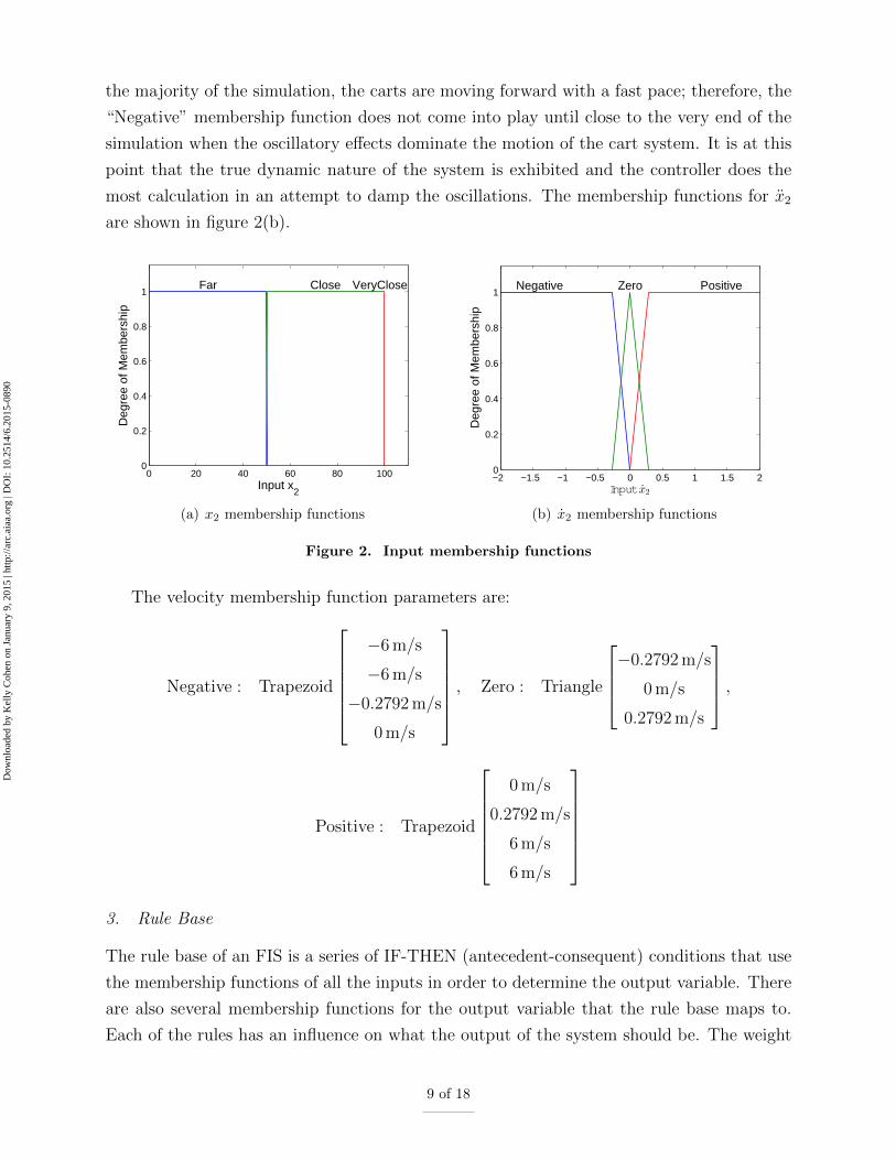
the majority of the simulation, the carts are moving forward with a fast pace; therefore, the

“Negative” membership function does not come into play until close to the very end of the

simulation when the oscillatory effects dominate the motion of the cart system. It is at this

point that the true dynamic nature of the system is exhibited and the controller does the

most calculation in an attempt to damp the oscillations. The membership functions for x2

are shown in figure 2(b).

0 20 40 60 80 1000

0.2

0.4

0.6

0.8

1

Deg

ree

of M

embe

rshi

p

Input x2

Far Close VeryClose

(a) x2 membership functions

−2 −1.5 −1 −0.5 0 0.5 1 1.5 20

0.2

0.4

0.6

0.8

1

Deg

ree

of M

embe

rshi

pInputx2

Negative Zero Positive

(b) x2 membership functions

Figure 2. Input membership functions

The velocity membership function parameters are:

Negative : Trapezoid

−6 m/s

−6 m/s

−0.2792 m/s

0 m/s

, Zero : Triangle

−0.2792 m/s

0 m/s

0.2792 m/s

,

Positive : Trapezoid

0 m/s

0.2792 m/s

6 m/s

6 m/s

3. Rule Base

The rule base of an FIS is a series of IF-THEN (antecedent-consequent) conditions that use

the membership functions of all the inputs in order to determine the output variable. There

are also several membership functions for the output variable that the rule base maps to.

Each of the rules has an influence on what the output of the system should be. The weight

9 of 18

Dow

nloa

ded

by K

elly

Coh

en o

n Ja

nuar

y 9,

201

5 | h

ttp://

arc.

aiaa

.org

| D

OI:

10.

2514

/6.2

015-

0890

of these influences again varies from 0 to 1 and the final output value is determined by

calculating the centroid of all of the rules. For instance, one rule dictates that if the car is

far away then the output force should be positive and large so that the car will move towards

the wall. Another rule will say that when the car is close to the wall the output force should

be negative in order to slow the car down. All of these rules have influence over all input

ranges determined by how the input variables map to the given membership functions in

that specific rule.

The antecedent of each statement contains memberships of both input variables and the

consequent maps to the output membership functions. The rules for this FIS were developed

based upon intuitive decision making. The rules developed for our FIS are shown in Table 1.

Table 1. Rule Base of the Fuzzy Inference System

Velocity Measurement

Negative Zero Positive

PositionMeasurement

Far Positive

Close Positive Zero Negative

VeryClose Positive Zero Negative

Control Force

4. Control Force

−2 −1.5 −1 −0.5 0 0.5 1 1.5 20

0.2

0.4

0.6

0.8

1

Deg

ree

of M

embe

rshi

p

Output Force

Negative Zero Positive

Figure 3. Control force

membership functions.

The output variable, force, is also composed of three mem-

bership functions. The output force is bounded from −1 N to

1 N thus the membership functions allow for the output to be

“Negative”, “Zero”, or “Positive”. As the centroid of the area

beneath each function is used to evaluate the control force,

the upper and lower bounds are centered over 1 and -1 respec-

tively. These functions represent the “defuzzification” stage of

the FIS and these outputs are determined by evaluating each

rule in the rule base (see § 3 on the previous page) in parallel.2

The controller emulates bang-bang control for the majority of

the simulation lifetime, sharply transitioning from full acceleration to full deceleration. As

the cart system nears the wall, the oscillation damping rules will dictate the force to apply

10 of 18

Dow

nloa

ded

by K

elly

Coh

en o

n Ja

nuar

y 9,

201

5 | h

ttp://

arc.

aiaa

.org

| D

OI:

10.

2514

/6.2

015-

0890

on the system. Typically, the output force will be directed opposite to the velocity of cart 2.

The membership functions for the control force are shown in figure 3 on the preceding page.

Negative : Triangle

−2 N

−1 N

0 N

, Zero : Triangle

−1 N

0 N

1 N

, Positive : Triangle

0 N

1 N

2 N

B. Simulation Performance

0 10 20 30 40 50

−1

−0.8

−0.6

−0.4

−0.2

0

0.2

0.4

0.6

0.8

1

Time (s)

Con

trol

ler

For

ce (

N)

Figure 4. System control

force over time.

The efficiency of this FIS was determined by using it as the

control mechanism in the simulation. The goal was to approach

the realistic theoretical limits calculated above and reach this

goal with minimum force. Table 2 shows the settling time, final

position of cart 2 and the calculated J value for the controller’s

performance. Figure 4 shows the controller’s output force over

time for each step of the simulation. The controller’s output

force is much lower than previously tested fuzzy solutions as

well as an optimal linear controller.

It is clear that the controller expends less energy than a

traditional bang-bang type controller would in the oscillation damping process. It can be

seen that the FIS responds quickly to control needs and applies the needed force with low-

latency.

Much work was done to hand-tune this controller to perform optimally, thus the work

was undertaken to develop a genetic algorithm to produce similar results autonomously.

Automating the tuning process ultimately produces a controller which is nearly as good as

the hand-tuned controller, but requires little to no effort from the programmer.

Table 2. Results from implemented FIS.

tf x2(500) J

32.303 s 99.999 821 m 0.32328

IV. Genetic Algorithm

The performance of the FIS depends directly on the value of each parameter of the

membership functions. These values were hand-tuned by a time-consuming process of

trial and error. To quicken this process, a genetic algorithm was utilized to autonomously

tune the membership functions and approach an optimal solution.

11 of 18

Dow

nloa

ded

by K

elly

Coh

en o

n Ja

nuar

y 9,

201

5 | h

ttp://

arc.

aiaa

.org

| D

OI:

10.

2514

/6.2

015-

0890

A genetic algorithm is a computational mechanism which imitates evolutionary behavior

to achieve optimality. It consists of a population of individuals which undergoes a process

similar to natural selection, reproduction, and mutation over the course of a number of

generations.4 Selection is attained by evaluating the fitness of each individual according

to a fitness function. For the purposes of this research, each individual represents a FIS

and the fitness function is simply the cost function used earlier. The individual which most

effectively minimizes the cost function is considered most fit for the control environment.

In order to manipulate the FIS structure in an algorithmic manner, it is necessary to

represent it as a genetic individual. Since the values of the parameters of the membership

functions of the FIS have significant impact on the control performance, it was decided to

manipulate only these parameters with the algorithm; however, of the thirty-one parameters

which comprise this FIS model, many are trivial to the overall performance. It is desirable

to reduce the number of parameters to facilitate the optimization process.

A. Parameter Reduction

To simplify the genetic tuning of the parameters, the symmetry of the system was exploited.

The parameters were reduced from thirty-one to seven. The position membership functions

were simplified to only three parameters by defining a center point (center) between far and

close functions, a distance from the center point at which the far and close functions will be

valued at 0 and 1 respectively (iTrap1), and half of the base of the triangular membership

function which decides when the car is very close to the wall (iTriBase1). The velocity mem-

bership function parameters were reduced to two parameters by defining the one parameter

for the distance from 0 that each of the membership functions reaches 1 for the negative and

positive functions (iTrap2) and another to define half of the base of the zero velocity triangu-

lar membership function (iTriBase2). The output force membership functions were reduced

similarly by allowing the negative and positive membership functions become trapezoidal

(oTrap and oTriBase).

• Position Membership Function Parameter

Far : Trapezoid

0

0

(center − iT rap1)

(center + iT rap1)

, Close : Trapezoid

(center − iT rap1(center + iT rap1)

99.9

100

,

12 of 18

Dow

nloa

ded

by K

elly

Coh

en o

n Ja

nuar

y 9,

201

5 | h

ttp://

arc.

aiaa

.org

| D

OI:

10.

2514

/6.2

015-

0890

VeryClose : Triangle

(100− iT riBase1)

100

(100 + iT riBase1)

• Velocity Membership Function Parameters

Negative : Trapezoid

−6

−6

(0)− iT rap2)

0

, Zero : Triangle

(0− iT riBase2)

0

(0 + iT riBase2)

,

Positive : Trapezoid

0

(0 + iT rap2)

6

6

• Control Force Membership Function Parameters

Negative : Trapezoid

−2

(−1− oTrap)(−1 + oTrap)

0

, Zero : Triangle

(0− oTriBase)

0

(1 + oTriBase)

,

Positive : Trapezoid

0

(1− oTrap)(1 + oTrap)

2

These Parameter reductions allow an individual to be defined by a single vector of seven

variables.

13 of 18

Dow

nloa

ded

by K

elly

Coh

en o

n Ja

nuar

y 9,

201

5 | h

ttp://

arc.

aiaa

.org

| D

OI:

10.

2514

/6.2

015-

0890

• Individual Definition

iT rap1

center

iTriBase1

iT rap2

iT riBase2

oTrap

oTriBase

B. Population Initialization

An initial population is generated by assigning random values to each of the individual

parameters within given ranges. iTrap1, iTriBase1, and oTriBase are allowed to vary between

0.05 and 1. iTrap2 and iTriBase2 are allowed to vary between 0.05 and 2. Center values

fall between 45 and 55, and oTrap between 0.05 and 0.95. Twenty individuals comprise a

population. Each individual is evaluated for fitness and brought up for selection to produce

a new generation.

C. Parent Selection and Reproduction

A new generation consists of three individuals which remain unchanged from the previous

generation, called elite children, ten individuals which are created from recombination of

two parents, five individuals which are created from mutating recombined children, and two

individuals randomly defined from the previously defined ranges.

Parents are selected by selecting the three best fit individuals to both become parents

and elite children. Seven more parents are selected by randomly choosing three individuals

from the remaining population, selecting the most fit, and returning the other two. This

tournament style of selection is repeated until all parents are selected.

Reproduction occurs by blended crossover process with an α modification (BLX-α), by

selecting a new parameter x′i from the range [xmin − Iα, xmax + Iα], where

xmin = min(x1i , x2i ) and xmax = max(x1i , x

1i )

Parents are defined as

C1 = (x11, x12, · · · , x17) and C2 = (x21, x

22, · · · , x27)

14 of 18

Dow

nloa

ded

by K

elly

Coh

en o

n Ja

nuar

y 9,

201

5 | h

ttp://

arc.

aiaa

.org

| D

OI:

10.

2514

/6.2

015-

0890

I =xmax − xmin

bi − aiα = min(d1, d2)

d1 = xmin − ai and d2 = bi − xmax

The interval [ai, bi] is the parameter-specific range. This mechanism allows the algorithm

to create a child from two parents which is a blend of both parents, while still expanding

the search space. As a population generally converges on a solution, so too do the children

of the population.

D. Mutation

Five of the recombined children are selected by random sampling and then two randomly

sampled parameters are selected from each of these child for mutation. Mutation is defined

to be nonuniform such that the mutation has a smaller effect in later generations as follows:

x′i =

ai + ∆(t, xi − ai), if τ = 0

bi −∆(t, bi − xi), if τ = 1

where τ represents a coin flip such that P (τ = 1) = P (τ = 0) = 0.5

∆(t, x) = x(1− λ(1− t

tmax

)b)

where t is the current generation, and tmax is the maximum number of generations. The

variable λ is a random value from the interval [0, 1]. The function ∆ computes a value in the

range [0, x] such that the probability of returning a zero increases as the algorithm advances.

The value of b determines the impact of the time on the probability distribution of ∆. The

value of b is set to 1.5 for algorithm for this research.

Two additional children are added to the population by random selection from the ranges

in order to ensure that the search space is sufficiently large.

V. Results

Running the algorithm for 50 generations yields a FIS which performs as well as the

hand-tuned FIS from B on page 11. This result converges out of the evolution process

quickly as can be seen in figure 5(a) on the following page. Though the algorithm finds

a near optimal solution quickly, it continues to search similar solutions, selecting the best

15 of 18

Dow

nloa

ded

by K

elly

Coh

en o

n Ja

nuar

y 9,

201

5 | h

ttp://

arc.

aiaa

.org

| D

OI:

10.

2514

/6.2

015-

0890

individuals each time to produce progressively better fit children each generation. Figure 5(b)

shows the average fitness of generation. It is clear from this plot that the algorithm produces

many unfit children in its search for optimality. This satisfies the need of a good algorithm

to expand the search area to eliminate premature convergence.

The results of the performance of the most fit individual produced by the genetic algo-

rithm are shown in Table 3.

Table 3. Final Results from algorithm-generated FIS

tf x2(500) J

32.308 s 99.999 999 m 0.32311

0 10 20 30 40 50

0.35

0.4

0.45

0.5

0.55

0.6

0.65

0.7

Generation

Mos

t Fit

Indi

vidu

al

(a) Best fit individual by generation.

0 10 20 30 40 500

50

100

150

200

250

300

350

Generation

Ave

rage

Fitn

ess

of P

opul

atio

n

(b) Individual fitness average by generation.

A. Genetic Adaptability

These results demonstrate the ability of the genetic algorithm to tune a FIS to near-optimal

performance. All tuning and development heretofore was done with an unchanging system

setup of known masses connected by a known spring. Although a robust controller,3 intro-

ducing changes to the masses of each car significantly alters the performance of the FIS as

it was carefully tuned to only a certain envelope; however, utilizing the genetic algorithm

to generate an optimum FIS for each new system setup is an efficient method of developing

good active controllers. This is demonstrated by changing the masses m1 and m2 to 2 kg

and 4 kg respectively. They are again changed to 4 kg and 8 kg, and finally 4 kg and 16 kg.

The algorithm was deployed for each case to optimize a controller for that envelope. After

fifty generations of evolution, the genetically optimized FIS performed within 3% of the the-

oretical rigid body limit in all four cases. These results are displayed in Table 4 on the next

page.

16 of 18

Dow

nloa

ded

by K

elly

Coh

en o

n Ja

nuar

y 9,

201

5 | h

ttp://

arc.

aiaa

.org

| D

OI:

10.

2514

/6.2

015-

0890

Table 4. Genetic algorithm FIS performance compared the hand-tuned FIS and rigid bodylimit.

Mass 1 (kg), Mass 2 (kg)

1 kg, 2 kg 2 kg, 4 kg 4 kg, 8 kg 4 kg, 16 kg

Theoretical Limit 0.3191 0.4553 0.6438 0.8312

GA FIS 0.3231 0.4562 0.6579 0.8434

Hand-tuned FIS 0.3230 0.6125 5.3072 3.3240

GA Error 1.3% 0.2% 2.2% 1.5%

Hand-tuned Error 1.2% 34.5% 724.4% 299.9%

It is easily seen in these results that the use of the genetic algorithm is advantageous

in the autonomous development of near optimal FIS controllers. Given a generic control

architecture, the genetic algorithm is able to tune a FIS rapidly and accurately for a varied

set of circumstances.

VI. Conclusions

Fuzzy logic provides a robust framework for control. It has been demonstrated that

proper fuzzy control is efficient and computationally inexpensive. The inherent vague-

ness of set membership and linguistic operation of fuzzy logic allows the controller to mimic

expert human control. This superior control, however, comes with a steep cost in FIS devel-

opment. Hand-tuning a FIS is time-consuming and tedious.

The use of the genetic algorithm facilitates FIS development. Once a FIS has been

developed for a general type of control situation, it is relatively simple to define the FIS as

a genetic element and automate the tuning through the evolutionary process. These results

imply that if a general fuzzy controller is developed for a family of control situations, then

a genetic algorithm can be implemented to tune each FIS to its specific task. The tuning,

therefore, can be accomplished by someone with no expertise in the control of the situation.

As the computation is quick, efficient control could be widely distributed due also to the

low-cost of development.

References

1Kosko, B., Fuzzy Thinking, The New Sciencs of Fuzzy Logic, Hyperion, NY, 1994.

2The MathWorks Inc, Natick, Massachusetts, United States, MATLAB and Fuzzy Logic Toolbox Release

2012b, 2012.

3Cohen, K., Weller, T., and Ben-Asher, J., “Control of Linear Second-Order Systems by Fuzzy Logic-

Based Algorithm,” Journal of Guidance, Control, and Dynamics, Vol. 24, No. 3, 2001, pp. 494–501.

17 of 18

Dow

nloa

ded

by K

elly

Coh

en o

n Ja

nuar

y 9,

201

5 | h

ttp://

arc.

aiaa

.org

| D

OI:

10.

2514

/6.2

015-

0890

4Cordon, O., Herrera, F., Hoffmann, F., and Magdalena, L., Genetic Fuzzy Systems, Evolutionary Tuning

and Learning of Fuzzy Knowledge Bases, World Scientific Publishing Co., MA, 2001.

5Walker, A., “untitled,” Class project.

6Stimetz, A., “untitled,” Class project.

7Mitchell, S., “untitled,” Class project.

8Vick, T., “untitled,” Class project.

9Kosko, B. and Isaka, S., “Fuzzy Logic,” Scientific American, , No. 269, 1993, pp. 76–81.

18 of 18

Dow

nloa

ded

by K

elly

Coh

en o

n Ja

nuar

y 9,

201

5 | h

ttp://

arc.

aiaa

.org

| D

OI:

10.

2514

/6.2

015-

0890