Genetic aspects of a small scale honeybee breeding program A thesis submitted to Bangor University for the degree of Doctor of Philosophy By Ian Williams May 2013 Molecular Ecology Laboratory Bangor University School of Biological Sciences Environment Centre Wales Bangor Gwynedd, LL57 2NU

Welcome message from author
This document is posted to help you gain knowledge. Please leave a comment to let me know what you think about it! Share it to your friends and learn new things together.
Transcript
Genetic aspects of a small scale honeybee
breeding program
A thesis submitted to Bangor University for the degree of
Doctor of Philosophy
By Ian Williams
May 2013
Molecular Ecology Laboratory
Bangor University
School of Biological Sciences
Environment Centre Wales
Bangor
Gwynedd, LL57 2NU

Part of the funding for this project was provided by the Knowledge Economy Skills
Scholarships (KESS) is a major European Convergence programme led by Bangor
University on behalf of the HE sector in Wales. Benefiting from European Social
Funds (ESF), KESS support collaborative research projects (Research Masters and
PhD) with external partners based in the Convergence area of Wales (West Wales and
the Valleys).
Extensive contributions were also made by Bangor University and Tropical Forest
Products Ltd. The West Wales Bee Breeding program was set up as a partnership
between the University and Tropical Forest, one of Wales’ largest bee farmers and
importers of organic African honey and beeswax, based in Ceredigion. The ultimate
goal of the project is be to produce a hardy, productive, strain of bees resistant to
varroa and other diseases without the use of medications.

I’r Hogiau
Cofiwch
‘Dyfal donc a dyrr y garreg’

i
Summary
Beekeepers in Wales, like others across the northern hemisphere, continue to experience
high overwintering colony losses. Breeding for local adaptation has been recommended as
part of the solution. The West Wales Bee Breeding Program (WWBBP) was therefore
established in an effort to improve, through selection, the resilience and production
potential of a local bee stock. Breeding for desired character traits began in 2011 and
focused mainly on colony strength, varroa mite infestation, and temperament. Foraging
efficiency was also monitored when conditions allowed. This thesis presents data from the
first two rounds of selection. Scant evidence indicating adaptive change due to selection
was detected across this time frame, but a demonstrable reduction in the variance of colony
strength was observed.
The influence of selection across generations on population level genetic variation was also
monitored. Microsatellite loci were highly polymorphic in the source population, and great
diversity was also observed at a custom csd marker. Low frequency alleles at both marker
types were lost across generations, and a significant difference in allelic richness was
observed between the source population and each of the following two daughter
generations. The effects of various selection/breeding parameters on the rate of genetic
depletion due to selection within a contemporary timeframe (5 generations) were
simulated, and the possible consequence of long term genetic depletion on adaptive
response was considered. Simulations indicated that the number of breeder queens selected
had the greatest influence on the rate of genetic depletion at both neutral loci and at the csd
locus, across years.
The WWBBP aims to enhance local suitability through selective breeding while
concurrently preserving genetic diversity and adaptive potential in the simplest most
practical way. Hopefully, this thesis will help guide the future development of the
program, and in addition, provide a basic transferable template for successful small-scale
breeding.

ii
Acknowledgments
I have been fortunate over the last few years to have experienced a world that many
know little about, and to have done so in region of the world so familiar to me. Many
deserve my appreciation and gratitude. First, I would like thank Anita Malhotra for her
work establishing this project, and for her support and guidance along the way.
Academic support was also provided by my guiding committee; Simon Creer and Henk
Braig. I thank Wendy Grail for her unwavering support and utmost professionalism in
the lab, and also Delphine Lallias who was always so approachable when I needed
assistance analysing my data.
I would like to thank David Wainwright, of Tropical Forest Products, for freely sharing
his beekeeping knowledge and expertise, and for allowing me to learn the skills of the
trade while working his bees. Thanks also to beekeeper Steve Benbow for providing
assistance setting up experimental colonies. Paul Davidson deserves recognition for
assisting me to set up my field weather stations, and for providing drone samples for this
thesis.
None of this work would have been possible without the support of my family, and
especially that provided by my wife, Anne H. Paley. She endured a personal battle, but
continued to encourage and believe. Thank you to my parents for all their help, and finally,
I would like to thanks my sons Dylan and Ryan for their support and resilience during this
time. I sincerely hope this project has made a positive contribution to the region.

iii
Table of Contents
Page
Summary i
Acknowledgments ii
Table of Contents iii-v
Glossary vi-vii
CHAPTER 1 General Introduction
1
1 Introduction 2
1.1 Ecological and Economic Role 2
1.2 Honeybee Health and Disease 3
1.2.1 Varroa 5
1.2.2 Mite resistance in honeybees 7
1.2.3 Nosema 8
1.2.4 Viruses 9
1.2.5 Pesticide Threats 11
1.3 Bee Translocations 13
1.3.1 Translocation within the endemic A. mellifera range 13
1.3.2 Translocations of A. mellifera into the native range of other Apis genera 14
1.3.3 Translocation of A. mellifera into regions with no indigenous Apis 15
1.4 Colony Life 15
1.5 Complementary sex determination gene csd 16
1.6 Bee Breeding 18
1.6.1 Hybrid Breeding 18
1.6.2 Line Breeding 10
1.6.3 Closed population breeding and selection 20
1.6.4 The West Wales Bee Breeding Program 20
1.7 Aims of the Thesis 24
CHAPTER 2 The mating frequency and flight behaviour of honeybee
queens on the edge of their natural distribution
25
Introduction
26-30
Results 30-34
Discussion 34-37
Materials and Methods 37-41
CHAPTER 3- Selection on Phenotype 45
3.1 Introduction 46
3.1.1 Breeding for Productivity 47
3.1.2 Selecting for varroa mite resistance 48
3.1.3. Other considerations relevant to honeybees 48
3.2 Methods 50
3.2.1 Grafting and raising queen cells 51
3.2.2 Making nuclei colonies 51
3.2.3 Measuring colony strength and foraging efficiency 53
3.2.4 Varroa mite counts 55
3.2.5 Measuring colony temperament 55
3.2.6 Data analysis and colony comparisons 55
iv
3.2.7 A comment on monitoring adaptive change 57
3.3 Results
3.3.1 Season 2011 57
3.3.2 2012 Season 57
3.3.3 Testing for difference in variance between years 59
3.3.4 Temperament 62
3.4 Discussion 64-70
CHAPTER 4 Selection on Genetics
71
4.1 Introduction 72
4.1.1 Avoiding inbreeding 72
4.1.2. Genetic variation in honeybee populations 73
4.1.3 Effective population size 74
4.1.4 Microsatellite loci and the complementary sex determination (csd) locus 74
4.2 Methods 75
4.2.1. Population genetic data sampling 75
4.2.2 DNA extraction 76
4.2.3 PCR multiplex systems 76
4.2.4 CSD-marker 77
4.3 Statistical Analysis 78
4.3.1.Overlapping Generations 78
4.3.2 Genetic diversity 78
4.3.3 Detecting bottlenecks 79
4.3.4 Estimating the effective population size (Ne) 80
4.3.4a Estimating Ne using single sample approaches 82
4.3.4b Estimating Ne using temporally based methods 82
4.3.5 Moment-based temporal methods 83
4.3.5a Coalescent based temporal method (TM3) 83
4.4 Results 83
4.4.1 Microsatellites (neutral markers) 84
4.4.2 Complementary sex determination (csd) 85
4.4.3. Bottleneck 86
4.4.4 Assessing Effective Population Size (Ne) 89
4.4.4a Single sample methods 89
4.4.4b Two sample temporal methods 89
4.5 Discussion 89-93
CHAPTER 5 Monte Carlo Simulations
5.1 Introduction 94
5.1.1 My model designs 95
5.2 Methods 97
5.2.1 Microsatellite methodology 98
5.2.2 csd methodology 99
5.3 Simulation Results 100
5.3.1 Microsatellites 100
5.3.2 Simulating csd (under WWBBP protocols) 105
5.3.3 Additional modeling of csd 107
5.4 Discussion 109
5.4.1 Selectively neutral markers 110
5.3.2 csd modeling 110
5.5 Summary/Recommendations 113
v
CHAPTER 6- CSD Variation
6.1 Introduction 116
6.1.1 Implication for breeders 118
6.1.2 Population screening 119
6.2 Methods 119
6.2.1 Sequencing haploids 120
6.2.2 Definition of csd alleles 120
6.2.3 Genotyping 121
6.2.4 Sequencing diploids 121
6.3 Results 122
6.4 Discussion 126-128
CHAPTER 7 Final Discussion
7.1 Mating success
7.2 Monitoring
7.2.1 Varroa
7.2.2 locating the queen
7.2.3 Production and colony strength
7.3 Genetic monitoring and modelling
7.4 Breeding
7.5 Considerations for breeders
7.6 A final thought
7.7 Further work
129-141
130
130
131
132
132
133
134
136
138
138
References 142-157
Appendix i Table A1-2011 colony monitoring tables 158
Appendix ii Table A2-2012 colony monitoring tables 160
Appendix iii Microsatellite Matlab Monte Carlo simulation code 162-182
Appendix iv csd Matlab Monte Carlo simulation code 183-246
Appendix v DGGE methods 247
vi
Glossary
Chalkbrood- A fairly common fungal brood disease caused by the Ascosphaera apis. Its
effect on the majority of hives is only slight but it can adversely affect small
colonies in the early spring.
Grafting- First performed by G.M. Doolittle, and described in his book Scientific
Queen Rearing, published in 1888. It is the process of artificially raising
queens by removing larvae of appropriate age (from a colony of choice) and
placing them in artificially made (beeswax or plastic) cell cups. Many larvae
can in this way be presented to a prepped queenless cell raising colony.
Strong cell raising colonies can raise up to 100 or more cells under optimal
conditions.
Nucleus- Nucleus colonies are small colonies that are created from larger colonies. The
name is derived from the fact that a nuc hive is centered around a queen - the
nucleus of the honey bee colony.
Split- A term used to describe the process of ‘splitting’ a large colony into two or
three separate colonies, each with equal amounts of brood and stores. The
original will retain the queen, while the others may be left with brood and
bees of appropriate age to raise a new queen. A ‘walk-away’ split is one way
beekeepers use to expand their operation.
Spotty-brood- This is a characteristic brood pattern that results from the removal of diploid
drones by workers in a colony headed by a poorly mated queen.
Supersedure- This is the process of naturally replacing an existing queen. Bees can sense
when an old queen is failing and will raise a replacement.
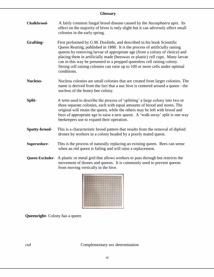
Queen Excluder- A plastic or metal grid that allows workers to pass through but restricts the
movement of drones and queens. It is commonly used to prevent queens
from moving vertically in the hive.
Queenright- Colony has a queen
csd Complementary sex determination
vii
He Expected heterozygosity
Ho Observed heterozygosity
Me Effective mating success
Nb Parental contribution from previous year
Ne (chapter 2) Estimated mating success
Ne (chapter 4) Effective population size
No Observed mating frequency
h2 heritability
V Brood viability
VP Phenotypic variance
VG Variance due to genetic effects
VE Variance due to environmental effects
VA Variance due to additive genetic effects

1
Chapter 1
General Introduction
2
1 Introduction
The Western honeybee, Apis mellifera (Hymenoptera, Apidae) is an old and highly
successful species. The development of colony life relaxed environmental constraints
allowing honeybees to expand across a broad range of climatic and ecological conditions
(Moritz et al., 2005). It adapted to arid sub-tropical conditions in the south, to cold
temperate conditions in the north, and its range extends across Western Europe from the
Atlantic coast of the Iberian Peninsula, to the Ural Mountains in the East. Correspondingly
diverse ecotypes evolved against this broad ecological background and there are currently
24-26 recognized ecotypes or subspecies (De la Rua et al., 2001; Moritz et al., 2005).
Morphological comparisons by F. Rutter, later supported by genetic analyses (Garnery et
al., 1992; Franck et al., 1998), collapse these sub-species into four distinct lineages (M, O,
A and C). Recent analyses of whole genome data propose an alternative to the previously
accepted hypothesis that the honey bee radiation initiated in Asia, suggesting instead, two
possibly separate out of Africa expansions and subsequent radiations (Whitfield et al.,
2006).
1.1 Ecological and Economic role
Honeybees play a critical role as angiosperm pollinators, and are of vital economic and
ecological importance (Genersch et al., 2010). Certain aspects of their biology make them
well suited for this purpose. They are generalists, able to forage and thrive on a wide range
of nectar and pollen sources, and to travel long distances to do so. Bees employ complex
communication behavior to pass information relating to location of nectar sources. They
are well suited to pollinate commercial crops. Thirty five percent of the food consumed by
people is pollinated by animals (Genersch et al., 2010), and the large-scale homogenized
agriculture practiced in Europe and the US requires pollination services from managed
honeybee apiaries. California exported $2.3 billion worth of almonds in 2010 alone, a crop
that is dependent upon the pollination services of honeybees. It is also claimed that
honeybees contribute between £200 million (British Beekeepers Association), and bees in
general up to £430 million pounds per annum (UK National Ecosystem Assessment) to the
British economy. Honeybees are responsible for pollinating a range of crops and are
responsible for pollinating 90% of the UK’s apple crops.
3
1.2 Honeybee Health and Disease
Honeybees live close social lives. They not only associate intimately with other members
of the colony, but are part of a community of organisms that may interact in beneficial,
neutral or antagonistic ways. They are susceptible to damage from a wide range of
metazoan, microbial and viral pathogens. Antagonists include: mites and beetles (Varroa
and Acarapis mites, and small hive-beetle); Microsporidia (Nosema apis and N. ceranae)
and other fungi; bacteria (American and European foulbrood); and viruses.
The bee population dramatically crashed in America over the winter of 2006-2007. These
collapse events were characterized by the sudden disappearance of adult bees, and with
apparent abandonment of hives, brood and food resources (vanEngelsdorp and Meixner,
2009). These symptoms collectively define colony collapse disorder (CCD), a newly
described specific collapse syndrome. Seasonal losses among managed colonies have
remained high since 2008. Preliminary survey results indicate that 31.1% of managed
honey bee colonies in the United States were lost this winter (2012/2013) (vanEngelsdorp
et al., 2013) and there was a critical shortage of bees for pollination on the almonds.
Although bumper crops are still expected (estimated to be over 2 billion pounds) due to
very good growing conditions, there is growing concern that ever diminishing bee numbers
may provide a problem for growers in the future.
Although CCD is recognized as a syndrome specific to North America, similar declines in
bee colonies were experienced in Europe. In France, the death rate was more than 60%
and England lost 30% of its colonies over the winter of 2007-2008 (Aston, 2010). No
single causative agent has yet been found. Worldwide incidents of unusually high levels of
colony deaths or “disappearance diseases” have been periodically reported (Table 1.1).
There have been 18 major episodes since 1869 (Underwood and vanEngelsdorp, 2007).
An infamous epidemic occurred in Britain during the early years of the 20th century. No
causative agent for the ‘Isle of Wight disease’ was isolated during the outbreak, and by
1919, Britain had lost 90% of its colonies. The microsporidian, Nosema apis, was
subsequently highlighted as a possible cause, as was the tracheal mite Acarapis woodi
(Neumann and Carreck, 2010). Chronic paralysis virus (CPV), identified in diseased Isle
of Wight bee samples by Lesley Bailey in the 1950’s, is now considered to be the most
likely cause of the outbreak (Allen and Ball, 1996; Bailey, 1964).
Other ‘disappearance’ outbreaks occurred in United States and Canada around 1920, and
again in the south and south western USA in the 1960’s (Underwood and vanEngelsdorp,
4
2007). Outbreaks of so-called ‘disappearing syndrome’ occurred in Australia and
‘disappearing disease’ in Mexico in 1975, with environmental factors determined to be
likely causes. Greater than average losses were reported in the United States during the
end of the 1970’s and again in the mid 1990’s (Underwood and vanEngelsdrop, 2007).
France experienced devastating losses between 1998 and 2000 with disease, stress due to
poor nutrition and chemicals in the environment being presented as possible contributors.
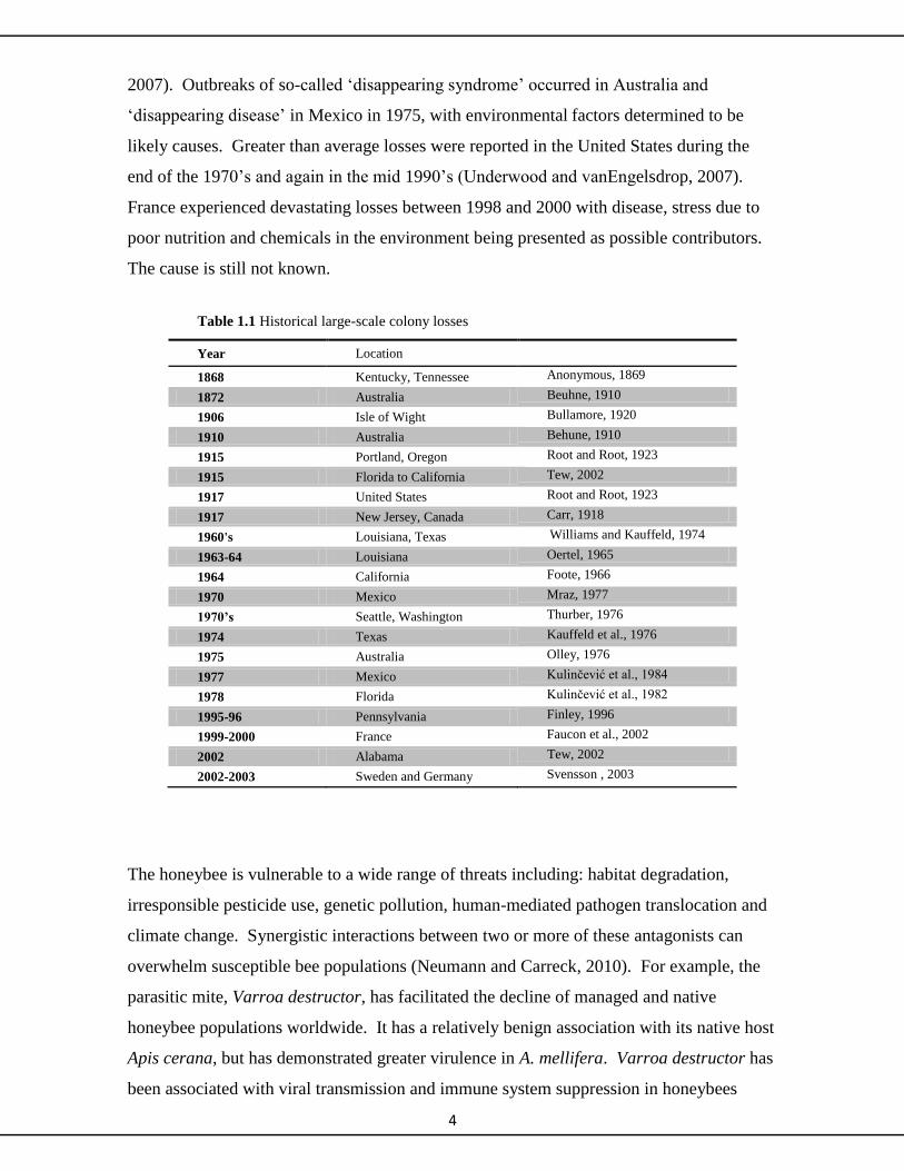
The cause is still not known.
Table 1.1 Historical large-scale colony losses
Year Location
1868 Kentucky, Tennessee Anonymous, 1869
1872 Australia Beuhne, 1910
1906 Isle of Wight Bullamore, 1920
1910 Australia Behune, 1910
1915 Portland, Oregon Root and Root, 1923
1915 Florida to California Tew, 2002
1917 United States Root and Root, 1923
1917 New Jersey, Canada Carr, 1918
1960's Louisiana, Texas Williams and Kauffeld, 1974
1963-64 Louisiana Oertel, 1965
1964 California Foote, 1966
1970 Mexico Mraz, 1977
1970’s Seattle, Washington Thurber, 1976
1974 Texas Kauffeld et al., 1976
1975 Australia Olley, 1976
1977 Mexico Kulinčević et al., 1984
1978 Florida Kulinčević et al., 1982
1995-96 Pennsylvania Finley, 1996
1999-2000 France Faucon et al., 2002
2002 Alabama Tew, 2002
2002-2003 Sweden and Germany Svensson , 2003
The honeybee is vulnerable to a wide range of threats including: habitat degradation,
irresponsible pesticide use, genetic pollution, human-mediated pathogen translocation and
climate change. Synergistic interactions between two or more of these antagonists can
overwhelm susceptible bee populations (Neumann and Carreck, 2010). For example, the
parasitic mite, Varroa destructor, has facilitated the decline of managed and native
honeybee populations worldwide. It has a relatively benign association with its native host
Apis cerana, but has demonstrated greater virulence in A. mellifera. Varroa destructor has
been associated with viral transmission and immune system suppression in honeybees
5
(Cox-Foster, 2007). The significance of the association between varroa and deformed
wing virus (DWV), and its influence on virus prevalence, load, and diversity, was recently
highlighted by Martin et al. (2012). They investigated how varroa affected the spread of
DWV in a newly colonized region (Hawaii in this case). They showed how the arrival of a
DWV strain that can replicate in varroa, led to the rapid spread and dramatic increase in
viral loads across the island. While the distribution and prevalence of other common
viruses remained unaffected, varroa radically and rapidly shifted the DWV viral
landscape.
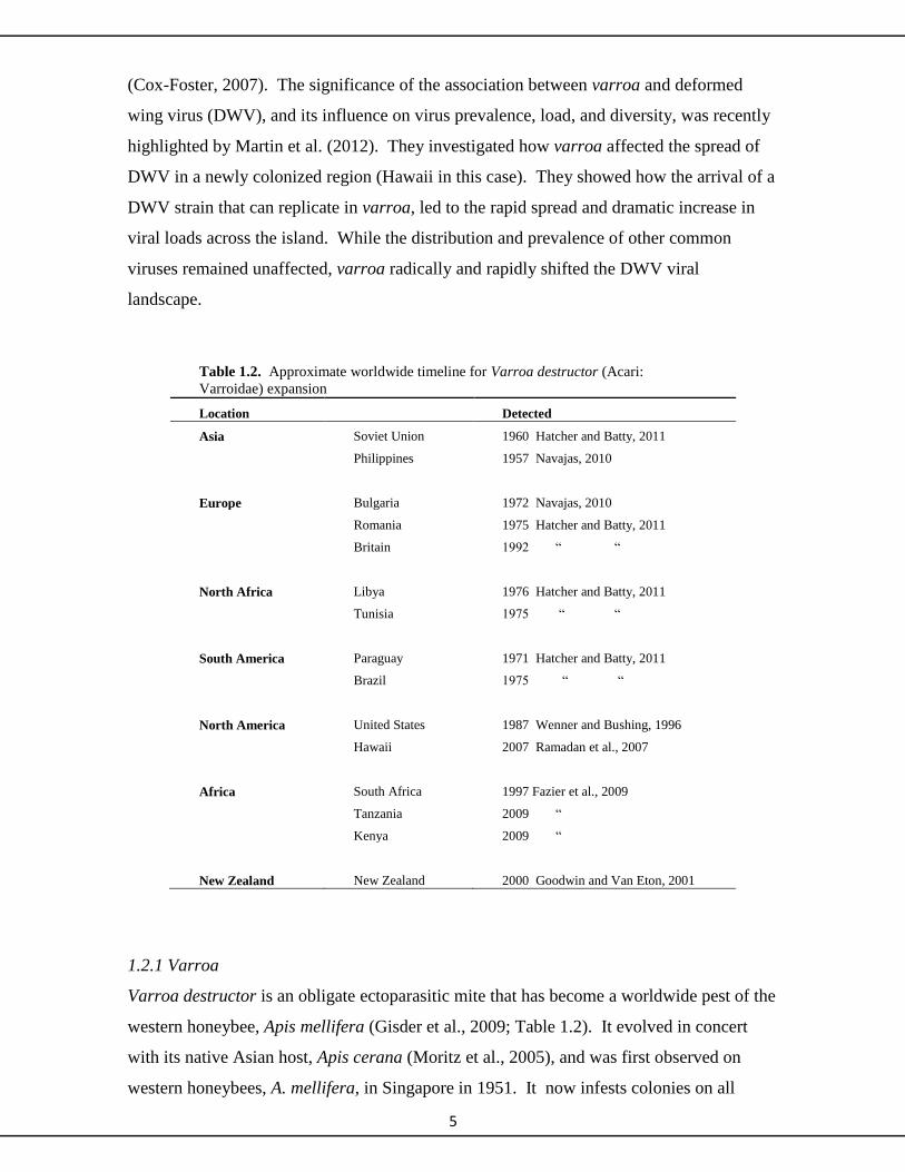
Table 1.2. Approximate worldwide timeline for Varroa destructor (Acari:
Varroidae) expansion
Location Detected
Asia Soviet Union 1960 Hatcher and Batty, 2011
Philippines 1957 Navajas, 2010
Europe Bulgaria 1972 Navajas, 2010
Romania 1975 Hatcher and Batty, 2011
Britain 1992 “ “
North Africa Libya 1976 Hatcher and Batty, 2011
Tunisia 1975 “ “
South America Paraguay 1971 Hatcher and Batty, 2011
Brazil 1975 “ “
North America United States 1987 Wenner and Bushing, 1996
Hawaii 2007 Ramadan et al., 2007
Africa South Africa 1997 Fazier et al., 2009
Tanzania 2009 “
Kenya 2009 “
New Zealand New Zealand 2000 Goodwin and Van Eton, 2001
1.2.1 Varroa
Varroa destructor is an obligate ectoparasitic mite that has become a worldwide pest of the
western honeybee, Apis mellifera (Gisder et al., 2009; Table 1.2). It evolved in concert
with its native Asian host, Apis cerana (Moritz et al., 2005), and was first observed on
western honeybees, A. mellifera, in Singapore in 1951. It now infests colonies on all
6
continents other than Australia. It was recently reported to be in East Africa, and is likely
more widespread across the continent (Fazier et al., 2009). By examining sequence
variation within the cytochrome c oxidase subunit 1 mitochondrial region (CO-I sequence
variation) and by using morphological comparisons of mites from around the world,
Anderson and Trueman (2000) demonstrated that V. destructor is part of a two-species
‘complex’ comprising of V. destructor and V. jabobsoni. Varroa jacobsoni occurs on its
native host A. cerana in Malaysia and Java, while V. destructor is found on A. cerana on
the Asian mainland and on other A. mellifera subspecies worldwide (Zhang, 2000). The
Asian honeybee, Apis cerana, co-evolved with varroa and employs innate behavioral
mechanisms (e.g., chewing out infested brood) to arrest colony infestations at manageable
levels. Additionally, mites cannot develop in A. cerana worker brood cells, and are limited
to the longer developing drone cells (Spivak, 1996) while drones weakened by parasitism
cannot emerge, hence both drone and mite die. In contrast, naïve populations of Apis
mellifera possessed no innate resistance to varroa and suffer alarming population declines
on initial exposure.
Varroa mites feed on the haemolymph of larvae, pupae and adult honeybees, during
different times of development, and numbers can proliferate to colony-lethal levels if
unchecked. Chemical suppression has been commonly employed in America and parts of
Europe. While successful in the short term, beekeepers have had to constantly revise their
chemical armory in response to chemical resistance developed by mites. After 20 years of
often haphazard chemical applications, mites in many countries have developed resistance
to much of what was used against them (e.g. pyrethroids such fluvalinate). Italian bees
became resistant to this class of chemicals in only 4 years and resistance rapidly spread
across Europe. More dangerous chemicals such as the organophosphate coumaphos
(PerizinTM
or AmitrazTM
) are no longer effective in some places (USA, France). Denmark,
in contrast to most nations, employed a nationally concerted response when varroa was
detected. Their approach limited chemical use. Apiaries were encouraged to remove
drone cells in the spring (varroa prefer drone cells since the longer drone development
time allows for better mite survival rates) and apply organic acids (formic and oxalic acid)
a couple of times a year. Sixty percent of Danish apiaries detected no varroa problems in
2005 with an additional 25% reporting mild infestation of a colony or two (Vejsnæs,
2005). However, with this all said, varroa is still a threat to Danish bees. Vejsnæs et al.
(Vejsnæs et al., 2010) describe losses of 30% in approximately 12,000 hives over the
7
winter of 2007-8. Favorable weather allowed varroa numbers to increase to lethal levels
in many colonies that winter.
1.2.2 Mite resistance in honeybees
Experience has demonstrated that resistant mite populations proliferate under the selection
advantage conferred on them by inappropriate chemical applications. An alternative
approach to the varroa problem has been the establishment of breeding programs selecting
for various varroa-resistant behaviours (Spivak, 1996; Rinderer et al., 2000). Marla
Spivak breeds bees that exhibit hygienic behavior (HYG), a two-step disease resistance
process performed by different bees within the colony. Some bees uncap infected calls,
while others remove the exposed (dead) brood from the hive (Gramachko and Spavik,
2003). Originally discovered as a response to American foulbrood, the behavior has
demonstrated effectiveness against the varroa mite (Spivak, 1996). Once considered to be
a simple two locus (one controlling capping and the other removal) “on or off’ trait, the
behavior is now recognized to be influenced by at least seven genes (Lapidge et al., 2002;
Wilkes and Oldroyd, 2002). Varroa sensitive hygiene (VSH) is a closely related behavior.
Bees exhibiting VSH can detect mite infested brood and uncap the cell to remove the live
brood, disturbing mite reproduction in the process (Boecking and Drescher, 1991; Rinderer
et al., 2000; Harris, 2007). The United States Department of Agriculture (USDA) has been
working with varroa-resistant strains of A. mellifera that adapted in sympatry with varroa.
European honeybees from the Ukraine were moved to the Primorsky region of Eastern
Russia, approximately 100 years ago. These bees adapted to varroa in a chemical free
environment and were the precursors of the varroa-resistant strains released for
commercial use in 2000 (Rinderer et al., 2000). Differential gene transcription analyses of
varroa-sensitive and non-sensitive bees indicated differences in olfactory and neural
sensitivity-associated genes (Navajas et al., 2008). Based on these observations, the
authors suggest that resistance to varroa is mostly behavioral. Identifying the location of
relevant loci has proven to be a challenging task since behavior traits are often under the
influence of multiple genes, and as previously noted, involves two separate behaviors
carried out by two different bees. Recent work from the Behaviour and Genetics of Social
Insects Lab, University of Sydney (Oxley et al., 2010) identified six quantitative trace loci
(QTL’s).
8
The South African experience is noteworthy since it has been postulated that the lack of
chemical intervention and increased hygienic behavior resulted in the observed population
rebound. The varroa mite (Varroa destructor) was detected into South Africa in 1997.
Although associated declines in native A. mellifera capensis and A. m. scutellata
populations occurred, no chemical intervention was adopted. After seven years of decline,
population numbers began to rebound, and varroa resistant proliferated (Fazier et al.,
2009). Losses due to varroa were recently described as incidental. African bees have
demonstrated naturally higher levels of hygienic behavior that other species of western
honeybee, demonstrating shorter brood time and greater tendency to swarm. Fries et al.
(2006) attempted a controlled version of the above natural ‘live and let die’ experiment.
They demonstrated co-adaption between host bees and mite over a six year period in an
isolated bee population of 150 hives. These hives were infested with varroa and left
untreated. Mite induced winter mortality dropped from 76% in the first year to 13 and
19% in the fifth and sixth years.
Some breeders also recognize the benefits of a more holistic approach to dealing with
parasites and disease. Continually medicating against varroa for example, can bolster and
help propagate disease susceptible strains. Population level tolerance can be enhanced by
breeding from the more mite-tolerant colonies, but treatments must be controlled so that
colonies with greater and lesser mite resistance can be distinguished. Some regions in the
northern hemisphere (e.g. Lleyn peninsula, Wales) are reporting limited mite mediated
losses and a concurrent reduction in varroacide use. Commercial beekeeping operations
are therefore reducing the use of medication in the production part of their operation, and
trying to eliminate treatment altogether in colonies selected for breeding. Research
indicates that a balance can develop in closed populations between mite virulence and bee
tolerance (possibly due to the viruses they vector) in un-medicated populations (Fries,
2009; Seeley, 2007). Locally adapted bees have demonstrated superior survivorship under
no-treatment regimes
1.2.3 Nosema
Microsporidia of the genus Nosema are specialized fungi that parasitize many kinds of
animals. Three species infect honeybees (Apis mellifera) and bumblebees (Bombus
terrestris) in the U.K.: Nosema apis, N. ceranae, and N. bombis. These parasites infect gut
epithelial cells, weakening individuals and colonies. Nosema apis causes dysentery.
Several viruses can transfer between individuals via contact and fecal contamination, and

9
are likely to associate with Nosema infection. These include: black queen-cell virus, bee
virus Y, and filamentous DNA virus (Ribiére, 2007). Nosema apis also causes disjointed
wings, increased winter die off rates and slow down of spring build-up of colonies.
Nosema ceranae was first observed in A. mellifera apiaries in Spain in 2006 (Higes et al.,
2006). It appears to be the most damaging of the two species (Paxton et al., 2007), having
the capacity to cause complete colony failure independent of any other infection (Higes et
al., 2009). Dysentery has not been reported as a symptom of N. ceranae infections (Fries,
2009). N. apis and N. ceranae are currently susceptible to treatment by fumagillin (Higes
et al., 2009). Although N. ceranae was statistically dismissed as a potential cause of
colony collapse disorder (CCD) in the United States (Cox-Foster et al., 2007), it was later
reiterated (Paxton, 2010) that the authors recognized that their study was not the best
approach to determining the causes of CCD since it was a snap-shot view only, and could
not track changes over time. Studies tracking colonies through time (Higes et al., 2009;
Martín-Hernanández et al., 2009) have reported mortalities resulting from N. ceranae
infection. Paxton (2010) also suggests that regional differences to sensitivity to nosema
may be due to differences in virulence among different strains of the micosporidian. It
seems that the role of Nosema in CCD has not yet been clearly elucidated.
1.2.4 Viruses
Viruses are important bee pathogens of great concern and interest to beekeepers and
researchers. Over 18 viruses are known to infect bees (Baker and Schroeder, 2008). Most
of the common viruses have single strands of positive sense RNA (Table 1.3). Colony life
provides a good environment for viral transmission. Viral transmission can occur
horizontally and vertically, either passing directly between individuals or from parent to
offspring in eggs and sperm (de Miranda and Genersch, 2010). Viruses can maintain
intergenerational host/parasite equilibriums through vertical transmission when hives are
healthy. Clinical signs of infection may be unobserved under such circumstances.
Alternatively, viruses pass horizontally among hive members during periods of stress,
passing into haemolymph after mite induced puncture, for example, or being ingested by
feeding and grooming in unhealthy hives. Nosema-induced dysentery may also aid the
viral transmission of BQCV and other viruses. Poor weather conditions can also aid viral
replication since hygiene condition may deteriorate within the hive as bees may not be able
to leave to defecate.
10
Viruses have been implicated in the several bee die-off and colony collapse incidences
(Bailey, 1964; Cox-Foster, 2007), and are known to associate with other bee parasites.
Black queen cell virus (BQCV) has been linked to Nosema, and deformed wing virus
(DWV) to Varroa. Paradoxically, DWV exhibits low virulence in Apis mellifera (de
Miranda and Genersch, 2010). More virulent bee viruses like chronic bee paralysis virus
(CBPV), acute bee paralysis virus (ABPV), Kashmir bee virus (KBV), BQCV, sacbrood
bee virus (SBV) may not be suitably vectored by varroa since they cause too rapid a
demise of its host colony (de Miranda and Genersch, 2010), and don’t allow enough time
for the mite to reproduce. The ‘classic’ varroa-DWV model recognizes that the negative
effects of DWV on bee health are a consequence of complex interactions between the mite,
bees, and the transmission pattern and virulence of the virus. Nevertheless, consistent
overwinter colony mortality resulting from DWV infection in the absence of mites was
recently reported (Highfield et al., 2009).
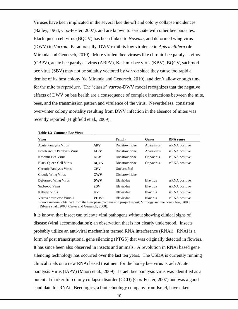
Table 1.3 Common Bee Virus
Virus Family Genus RNA sense
Acute Paralysis Virus APV Dicistroviridae Aparavirus ssRNA positive
Israeli Acute Paralysis Virus IAPV Dicistroviridae Aparavirus ssRNA positive
Kashmir Bee Virus KBV Dicistroviridae Cripavirus ssRNA positive
Black Queen Cell Virus BQCV Dicistroviridae Cripavirus ssRNA positive
Chronic Paralysis Virus CPV Unclassified
Cloudy Wing Virus CWV Dicistroviridae
Deformed Wing Virus DWV Iflaviridae Iflavirus ssRNA positive
Sacbrood Virus SBV Iflaviridae Iflavirus ssRNA positive
Kakugo Virus KV Iflaviridae Iflavirus ssRNA positive
Varroa destructor Virus 1 VDV-1 Iflaviridae Iflavirus ssRNA positive
Source material obtained from the European Commission project report; Virology and the honey bee, 2008
(Ribière et al., 2008; Carter and Genersch, 2008).
It is known that insect can tolerate viral pathogens without showing clinical signs of
disease (viral accommodation); an observation that is not clearly understood. Insects
probably utilize an anti-viral mechanism termed RNA interference (RNAi). RNAi is a
form of post transcriptional gene silencing (PTGS) that was originally detected in flowers.
It has since been also observed in insects and animals. A revolution in RNAi based gene
silencing technology has occurred over the last ten years. The USDA is currently running
clinical trials on a new RNAi based treatment for the honey bee virus Israeli Acute
paralysis Virus (IAPV) (Maori et al., 2009). Israeli bee paralysis virus was identified as a
potential marker for colony collapse disorder (CCD) (Cox-Foster, 2007) and was a good
candidate for RNAi. Beeologics, a biotechnology company from Israel, have taken

11
advantage of the RNAi mechanism to develop anti-viral treatments for bees. They claim to
have developed a treatment that offers potent protection from the following bee viruses:
Israeli acute paralysis virus (IAPV), Kashmir bee virus (KBV), black queen cell virus
(BQCV) and deformed wing virus (DWV).
The most common bee viruses are RNA-based (Table 1.3). Polymerase Chain Reaction
(PCR) technology allows for detection and quantification of viral activity in bees. Bees
can be screened for specific viral infection by applying reverse transcription of viral-
specific mRNA, followed by amplification and visualization of the resulting cDNA. Baker
and Schroeder (2008) demonstrated that the RNA dependent RNA polymerase (RdRp)
gene can reliably distinguish between viruses within the Picornavirales, an order that
includes many of the common bee viruses. They also suggest that DWV, VDV-1 and KV
from the genus Iflavirus, are variants of the same virus and that care should be given in
using species-specific’ primer sets within that genus. Real-time quantitative PCR
technology allows viral loads to be quantified. This procedure detects material that is only
produced when the virus is actively replicating, indicating that an active infection is
occurring. The detection and quantification of replicated negative strand RNA would
suggest a true infection is occurring as opposed to passive viral transmission (de Miranda
and Generch, 2010; Gisder et al., 2009)
1.2.5 Pesticide Threats
Due to the nature of farming in Wales, local honeybees are not likely to be greatly affected
by pesticides. Nevertheless, bees are susceptible to pesticides and recent work on the
honeybee genome has shown that relative to other insects, they have fewer genes coding
for detoxifying enzymes (Claudianos et al., 2006). Recent worldwide developments have
also highlighted concern regarding the increasing use of neonicotinoids, a specific class of
pesticides. Neonicotinoid treated seeds offer systemic protection to the developing plant,
and are now commonly applied to many commercially important crops (e.g. corn, oil seed
rape, sunflowers) on an industrial scale. All parts of the plant (including pollen and nectar)
are pesticide laden. A coalition of beekeepers and environmental groups recently sued the
United States Environmental Protection Agency (EPA) for approving the registration of
Clothianidin and Thiamethoxam, claiming that these neonicotinoids cause severe damage
to bees and are the primary cause of colony collapse disorder (CCD). Recent scientific
publications have provided evidence supporting such claims. A high profile paper by
12
Schneider et al. (2012) described how neonicotinoids induced CCD like symptoms
(including a vacated and empty hive) in experimentally exposed colonies. Neonicotinoids
are acetylcholine receptor agonists that bind irreversibly causing hyper-stimulation of the
nervous system. These effects adversely affect the brain function and thought that foraging
field bees become disoriented and fail to return to the hive.
Another recent high impact paper claimed that field concentrations of neonicotinoid
pesticides can detrimentally affect queen health and the development of bumble bee
colonies under laboratory conditions (Whitehorn et al., 2012). There is a growing body of
evidence implicating pesticide use with pollinator loss, and on the April 29th 2013, the
European Union responded by voting to enforce a 2 year ban on the use of three type of
neonicotinoids on flowering plants, though eight (including the UK) of 27 member states
voted against the ban, and four abstained. Those doubting the ban claimed that scientific
evidence is currently inconclusive and that a complete embargo is unwarranted.
Opinions are similarly divided among the beekeeping community. Some commercial
operators have observed no adverse effect on their bees while foraging on neonicotinoid
treated crops, and claim that lack of varroa mite control and poor forage quality due to
shifts in climate patterns and agricultural practices are more impactful causes of colony
loss. Randy Oliver, a scientifically trained commercial beekeeper from California
(scientificbeekeeping.com), recently wrote a critique of the Schneider et al. paper (Oliver,
2012). He questioned both the methodology used (which involved very high neonicotinoid
loads presented to the experiment colonies) and their interpretation of results. He suggests
that the observed colony losses could have resulted from ineffective mite control, rather
than from pesticide poisoning. He presented these concerns in writing to the authors but
has yet to receive a response. A contrasting opinion is presented by another group of
American commercial operators, some of whom lost up to 70% of their colonies this
winter. The journalist Dan Rather (2013) reported on the resulting shortage of bees for
almond pollination in California this spring. Neonicotinoid pesticides were considered by
many to be a major contributing factor affecting declining bee health.
Chemical treatment has also been the prescribed response by many to varroa mite
infestation. Varroa frequently developed resistance, necessitating the use of novel
chemical treatments. Some of these chemicals could accumulate in the hive with time and

13
have unwanted effects at the higher concentrations. New treatments are developed in
response. The arms race continues in large scale bee operations.
1.3 Bee Translocations
The western honeybee evolved across a wide range of ecological and climatic conditions
(Moritz et al., 2005). Separate races or sub-species became regionally adapted, developing
regionally specific phenotypic and behavioral characteristics suited to particular
environments and conditions. Technological developments allowed bees to be distributed
away from their endemic ranges. Moritz et al. (2005) describe three kinds of human
mediated distributions: spread of A. mellifera within the ranges of other A. mellifera sub-
species (Europe, Western Asia and Africa); distribution of A. mellifera sub-species in
regions where other species of the genera Apis were found (Asia); and translocations into
areas not endemic to honeybees (Americas and Australia).
Foreign ecotypes (sub-species) exhibiting ‘superior’ traits have been introduced into the
UK over the years in an effort to enhance beekeeping productivity. Queens under natural
conditions mate on the wing some distance from the nest. They can therefore come into
contact with drones distant colonies. Consequently, both the managed and wild British
honeybees are probably of mixed genetic backgrounds. The plight and condition of native
bee populations is presently unclear. The introduction of Varroa destructor was
undoubtedly detrimental. At worst, the combined effects of disease and the introgression
of genes from introduced bees may have resulted in the extirpation of the native bee.
Nevertheless, bee colonies are cryptic and hard to locate, and locally adapted wild bees that
are in ‘balance’ with the parasite, may exist in some remoter parts (Jensen et al., 2005;
Villa et al., 2008). A number of regional bee breeding cooperatives are attempting to
identify and conserve these bees.
1.3.1 Translocation within the endemic A. mellifera range
Beekeepers have moved bees around the world in an effort to enhance desired beekeeping
traits. Since bee reproduction is difficult to control, introgression of genes from introduced
into native bee population can easily occur, resulting in the breakdown of locally adapted
gene complexes. In addition, areas can be flooded with managed queens of limited genetic
variation. Lack of genetic variation would weaken population level response to
environmental threats, and result in poorly mated queens (mated with few individuals or

14
closely related individuals). Hives with poorly mated queens have less resistance to
pathogenic infection (Baer and Schmid-Hemple, 1999; Hughes and Boomsma, 2004;
Seeley and Tarpy, 2007). Although the integrity of regionally co-adapted gene complexes
have been challenged by bee translocation, research suggests that autochthonous sub-
species can still be found in parts of Europe (De la Rua et al., 2001, 2002, 2003; Jensen et
al., 2005; Strange et al., 2007). In addition, notable efforts have been made to preserve
native strains. The Danish government implemented conservation measures to protect the
endemic “black” honeybee on the island of Læsö. Introgression of non-native genetic
material has occurred as a result of illegal importation of other A. mellifera sub-species
(Jenson et al., 2005).
Two sub-species of A. mellifera are endemic to South Africa, A. m. capensis, and A. m.
scutellata. Translocation of A. m. capensis into the native range of A. m. scutellata for
commercial beekeeping purposes resulted in rapid disappearance of the A. m. scutellata
colonies (Neumann and Hepburn, 2002). Apis mellifera capensis workers parasitized A.m.
scutellata hives, superseding native queens, and took over colonies by becoming layers
(Neumann and Hepburn, 2002; Moritz et al., 2005). Commercial beekeepers suffered great
losses, but native wild A.m.scutellata have to date been relatively unaffected
1.3.2 Translocations of A. mellifera into the native range of other Apis
Apis mellifera has become popular with Asian beekeepers, causing considerable decline in
use of the native A. cerana (Moritz et al., 2005). Hybridization can occur in both
directions between the species (Moritz et al., 2005). The negative consequences of
hybridization have been well documented (Allendorf et al., 2001). Hybridization between
these two species results in reduced fitness since queens of either species will be poorly
mated resulting in the waste of reproductive resources (Moritz et al., 2005). The hybrid
juveniles are inviable; hence locally adapted A. cerana gene complexes stay intact. The
transfer of the parasitic mite Varroa desctructor from its native host A. cerana, into naïve
A. mellifera populations, initiated the most devastating plague of the western honeybee
(Moritz et al., 2005). Its spread has highlighted in a dramatic way the unintended
consequence and dangers of ill-informed translocations. Nosema ceranae is also thought
to have recently transferred from A. cerana to A. mellifera and is expressing increased
virulence in its new host (Fries, 2009). Significant colony losses recently reported in Spain
were attributed to N. ceranae parasitism.

15
1.3.3 Translocation of A. mellifera into regions with no indigenous Apis
There are no honeybees endemic to the Americas and Australia. The first American
honeybees were probably British black bees (Apis mellifera mellifera) which landed in
Jamestown in 1622 (Delaney et al., 2009). Feral bees moved west across the continent to
the eastern slopes of the Rockies. No bees made it across the mountains. The first
honeybees to make west of the Rockies arrived in California by boat in the 1850’s. Most
honeybees (A. m. carnica and A.m. ligustica) were imported between 1859 and 1922.
Importation of bees into the US was outlawed in 1922 in response to the ‘Isle of Wight’
disease that had decimated British bee stocks. The ruling limited genetic variation in
available breeding stocks. It is thought that the progeny of all the commercial hives in the
US were bred from only 500 breeder queens (Delaney et al., 2009). Low levels of genetic
diversity correlate with reduced disease resistance, colony strength and overall colony
fitness in bees and other social insects (Tarpy, 2003). In addition, genetically similar
colonies are less buffered against disease transmission between colonies, and are at greater
risk of high colony losses.
1.4 Colony Life
The type of advanced colonial structuring that is observed in honeybees is termed eusocial.
It is characterized by cooperation between individuals in brood care and nest construction,
overlapping generations, and reproductive division of labor (Wilson and Holldobler, 2005).
A normally functioning honeybee colony may have 60,000 or more individuals, consisting
mostly of female workers that perform within and outside hive tasks such as brood care
(nursing), nest defense and foraging. Workers also tend to the queen, the prolific egg-layer
and mother of the colony, whose task it is to encourage colony growth and ultimately
reproduction through swarming. Each colony will also contain males (drones) at certain
periods of the year. Far fewer in number than workers, they are specifically adapted to
detect, catch, and mate with queens during their nuptial flight(s). Drones mate only once.
Virgin queens undertake one to three mating flights within the first few weeks of life,
mating with multiple males (drones), and storing the sperm for lifetime use and storage.
The mean paternity frequency (i.e. actual number of matings) for A. mellifera is around 13
(Cournet et al., 1986; Estoup et al., 1994). Seeley and Tarpy (2007) demonstrated that
colonies with higher levels of genetic variation (i.e. greater number of patrilines) were less
affected by American Foulbrood inoculation than colonies formed by single mated queens.
Baer and Schmid-Hempel (1999) reported similar results with bumblebees (Bombus
16
terrestris L.) with greater genetic variation correlating with reduced pathogen loads and
better reproductive success (see also Hughes and Boomsma 2004; Palmer and Oldroyd,
2003).
Extreme polyandry (>2 matings per queen) is relatively rare among the highly eusocial
insects (Tarpy and Page, 2000). It occurs in a few wasps, ants and bee genera, and has
been the topic of much debate, since it is not intuitively obvious what selective
advantage(s) is confers. Polyandry reduces the degree of relatedness among colony
individuals and exposes the queen to environmental (predatory and pathogenic) threats
(Tarpy and Page, 2001). In addition, within hive genetic heterogeneity has been correlated
with greater thermoregulation efficiency. Controlled experiments demonstrated that
genetically diverse colonies (greater number of patrilines) displayed greater thermal
stability in response to environmental change that genetically poor ones (Jones et al.,
2004).
1.5 Complementary sex determination gene csd
Sexual development in Hymenoptera is directed by a specific genomic region (Sex
Determination Locus; SDL) found on chromosome 3. Within this locus resides the
complementary sex determination gene (csd), whose protein product initiates the
development of males (usually haploid) in the default state. However, when the protein
product of two functionally distinct alleles combine (i.e. in diploids), another gene within
the SDL (fem) is switched and the process of feminization is triggered. Feminization
occurs only when csd alleles differ in diploids; homozygotes develop into sexually in-
viable diploid drones and are ‘cannibalized’ at an early developmental stage by workers.
Strong frequency dependent selection and heterozygote advantage promote high gene
variance at the locus. High levels of polymorphism are observed due to these forces
(balancing selection) since alleles tend to persist in evolutionary terms.
The population dynamics of the csd is of relevance to the bee breeder since colonies with
low brood viabilities due to unacceptably high levels of diploid drone production will be
less productive. Queens mate multiple times, and the probability that she will mate with a
drone carrying an identical allele to one of the two she carries is , where k = the
number of alleles in the population (assuming each is present in equal proportions). From
this relationship Page and Marks (1982) deduced that the brood viability (V) of a queen
that mates n times, with y of those drones carrying alleles that matched one of her own, is,
17
This relation assumes that each drone has an equal probability of mating and provides an
equal amount of sperm. In addition, the expected brood viability in a population closed to
the influence of migration will be
The expected mean brood viability is therefore higher in population carrying higher
numbers of distinct alleles since the probability of identical alleles matching in zygotes is
reduced. In addition, the mean population mating success (mean number of drones each
queen mates with) affects the variance in population level brood viability, but not the mean
itself (Cook and Crozier, 1995), with lower mating success resulting in greater variance in
brood viability. Number and frequency of distinct alleles (k) are important population
level criteria affecting diploid drone production. In general the industry considers brood
viabilities of less than 85% as unacceptable (Page and Marks, 1982). Beekeepers trying to
direct adaptive change by selecting a limited number of breeders each year will limit the
transfer of gene variation across generations, by they must concurrently maintain the
number and frequency of sex alleles to maintain an acceptable levels of brood viability in
the long term.
The molecular mechanisms of single locus sex determination are not completely
understood. It is not yet known for example, how one csd allele differs from another. A
hypervariable region (HVR) located in region 3 of the gene most likely holds the key to
unravelling this riddle (Cho et al., 2006). The HVR can be described as a pseudo-
microsatellite since it is comprised of short repetitive sequences, bounded by an arginine
and serine rich region on one side, and a proline rich region on the other. These more
conserved bordering regions were targeted by PCR in this study to investigate fragment
length variation within the HVR. One hypothesis suggests that the number of HVR
sequence repeats characterize csd allele function, and that differing numbers of repeats at
this coding region result in protein products of correspondingly differing lengths and
possibly function (Cho et al., 2006).
1.6 Bee Breeding
1.6.1 Hybrid Breeding

18
Selective breeding methods have been adopted for centuries to improve agricultural strains
of plants and animals. More recently, the genetic influences underlying the beneficial
effects of heterosis (hybrid vigour) have become better understood and recognized by plant
and animal breeders (Shull, 1948). Beekeepers have also realized the potential benefits of
out-crossing and the method has been successfully applied to improve stock vigor (Cale
and Gowen, 1956). However, since hybrid breeding requires the long term and costly
maintenance of pure inbreed lines, such efforts usually required the resources of large
commercial operations or research facilities. The Starline and Midnite bees were once
popular commercial four line hybrids produced by Dadant and Sons, Inc. (United States);
each was continually improved by the addition of new hybrid lines. Advancements in
Instrumental Insemination (II) methodologies (Laidlaw, 1944; Mackensen, 1947) allowed
breeders to maintain and cross genetically isolated lines through artificial mating. The
technique continues to be used to control mating. It does require some specialized
equipment and training; hence it is mostly used by professional breeders and research
establishments.
1.6.2 Line Breeding
A more commonly used approach is line breeding. Line breeding has been used since the
middle of the nineteenth century by European and American breeders. Most famously in
the UK, brother Adam of Buckfast Abbey developed the Buckfast line through many years
of cross-breeding different lines of geographical sub-species. He did this using open
mating partly in response to colony losses from the Isle of Wight disease during the early
part of the 20th century. Contemporary breeders mostly use line breeding to strengthen
honeybee stocks by encouraging the propagation of beneficial traits within the gene-pool.
A model line breeding program (The Russian Bee Breeding Program) was established by
the United States Department of Agriculture (USDA) in the 1990’s. The program was
transferred, with federal support, to the commercial sector and is currently maintained by
the Russian Honeybee Breeders Association, Inc. Seventeen lines, divided into three
separate blocks A, B, and C, are currently maintained. Blocks are comprised of a number
of independent beekeepers, each maintaining no more than two lines. An intricate
breeding design (Fig1.1) has ensured that inbreeding effects are minimal, both within the
program, and within the stock provided for commercial sale.

19
Figure 1.1. Each year, members will select the best looking colonies from each of their
lines as breeders. Their daughter colonies will be mated by drones sourced by queens
donated from the other two blocks. For example, a beekeeper maintaining lines in block A
will mate his virgin queens with drones produced by queens provided by all the members
of block B and C. A large number of daughter colonies are raised, and these are also
distributed among the other blocks for monitoring different environmental conditions. In
order to limit detrimental inbreeding effects, queens are made available for commercial
sale from each block only every third year.
Table 1.4 Bee breeding programs
Breeding Programs
Conservation
Conserving the Dark Bee in Europe http://www.gbbg.net/
Conserving the European Dark Bee,
Germany http://www.apis-mellifera-mellifera.de/
Saving the Dark Bee in Switzerland http://www.mellifera.ch/
Bee improvement in Cornwall http://www.westcornwallbka.org.uk/member/
Bee improvement and Breeders
Association http://www.bibba.com/
Disease Resistance Programs Russian honey bee (Ontario, Canada) https://www.uoguelph.ca/ses/users/eguzman
Minnesota Hygienics Program http://www.glenn-apiaries.com/hygienic_italian_
Russian Honeybee Project (US Dep.
Agri.) http://www.ars.usda.gov/Services/docs.
Varroa-tolerance New Zealand http://www.biosecurity.govt.nz/publications/biosecurity-
magazine
There are numerous programs adopting similar approaches worldwide (Table 1.4). Some
programs prioritize the enhancement of autochthonous phenotypes, believing that locally
adapted bees are better suited to regionally specific environments. For example, the
20
widely introduced Italian bee (A. m. ligustica) may not be well suited to forage and
overwinter in temperate northern European climates
1.6.3 Closed population breeding and selection
Closed population breeding is the process of selecting for specific required traits from a
closed population of bees. Closed populations are genetically isolated, and can be thought
of as a single line. Populations can be large or small, and more or less closed (Kulinčević,
1986), and various selection strategies (e.g. mass, random, within-family) can be employed
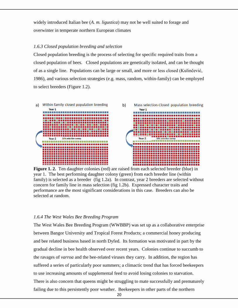
to select breeders (Figure 1.2).
Figure 1. 2. Ten daughter colonies (red) are raised from each selected breeder (blue) in
year 1. The best performing daughter colony (green) from each breeder line (within
family) is selected as a breeder (fig 1.2a). In contrast, year 2 breeders are selected without
concern for family line in mass selection (fig 1.2b). Expressed character traits and
performance are the most significant considerations in this case. Breeders can also be
selected at random.
1.6.4 The West Wales Bee Breeding Program
The West Wales Bee Breeding Program (WWBBP) was set up as a collaborative enterprise
between Bangor University and Tropical Forest Products; a commercial honey producing
and bee related business based in north Dyfed. Its formation was motivated in part by the
gradual decline in bee health observed over recent years. Colonies continue to succumb to
the ravages of varroa and the bee-related viruses they carry. In addition, the region has
suffered a series of particularly poor summers; a climactic trend that has forced beekeepers
to use increasing amounts of supplemental feed to avoid losing colonies to starvation.
There is also concern that queens might be struggling to mate successfully and prematurely
failing due to this persistently poor weather. Beekeepers in other parts of the northern
a) b) a)

21
hemisphere have consistently stated prematurely failing queens as a main reason for
overwintering losses (vanEngelsdrop et al., 2008, 2011, 2012). Honeybee queens mate
multiply on the wing, usually some distance from the nest, and will do so more
successfully during good weather. Young sufficiently mated queens tend to develop into
healthier, more vigorous and longer lived individuals than less successfully mated queens.
Queen mating success has been shown to influences the long term development and
performance of colonies (Richard et al., 2007; Tarpy et al., 2012).
Commercial beekeeping has become an increasingly risky proposition due to declining
bee-health. In response, some beekeepers have strived for sustainability by breeding from
locally proven productive stocks, rather than relying on imports to replace losses. Strange
et al., (2007) showed how bees adapted to regionally specific nectar flows, are ill-prepared
when moved to areas where peak nectar flows occurred at different times. Much of the
managed bee stock is now of mixed genetic heritage, and may therefore not be well suited
to all regions. Bees that evolved in northern climates for example, delay brood expansion
until late spring. Hybrids tend to expand earlier in the year and are more susceptible to
starvation if weather conditions turn unexpectedly cold. Hybrid queens cannot adjust their
egg-laying in response to weather and their colonies may not be able to survive without
supplemental feeding (Le Conte and Navajas, 2008). Honeybees have evolved in a broad
range of environments, and breeders hope to take advantage of this innate diversity
(plasticity and genetic) to breed for local adaptation (Le Conte and Navajas, 2008).
The challenge for the WWBBP was to design a purposeful breeding program that could be
integrated into the management framework of an existing small commercial operation.
Within this context, the aim was to start developing a breeding protocol that could
maintain a self-sustaining and productive population over the long term. There are no
fixed or defined end points or goals; only a process that enhances the resilience of bees to
be responsive to ever-shifting climate and disease challenges. It is an applied long term
project hoping to improve the commercial quality and regional specificity of a managed
honeybee stock.
The breeding program started in the spring of 2011. Tropical Forest bees suffered high
mortality over the 2010/11 winter and priority was given that summer to re-building
colony numbers. An estimated 43% of the Welsh colonies succumbed, with varroa mite

22
infestation deemed to be the major contributing factor. Potential breeders were selected
from overwintered survivors dispersed in apiaries up and down the Dyfi valley (mid-
Wales). The situation offered a breeding opportunity since a large number of new colonies
(n = 118) were needed to recoup losses. This was a rather unusual situation, since this
many replacement colonies are not normally required. The business accommodates at
most two hundred colonies in mid-Wales and experiences roughly 30% loss (60 colonies)
each year.
Beekeepers use various techniques to replace losses. Unfortunately, each method requires
dividing (splitting-glossary) the resources of strong colonies, regressing their progress and
future production potential in the process. The ‘old’ reduced colony usually retains the
original queen. All ’new’ colonies require new queens which can be acquired through a
number of different ways. Queenless splits can be left unattended near the original hive
with eggs and/or brood of appropriate age so that the bees can raise new queens (walk-
away split). Alternatively, the splits can be relocated and provided with an already mated
laying queen, or a ripe queen cell from which a virgin will imminently emerge. None of
these approaches provide immediate fixes since each new colony can take a season, if it
survives, to mature into production size in the UK. These are familiar beekeeping
practices that have been used by beekeepers managing sustainable programs to replace
expected seasonal losses. But increasingly severe losses result in more strong production
hives having to be sacrificed to make up colony numbers. Managing bees for honey
production has become increasingly difficult in the UK and is in danger of becoming
commercially unsustainable.
Having timely access to well-developed and genetically appropriate queens can provide
commercial operators with greater management flexibly. Replacement queens of reliable
stock are not readily or cheaply available in the UK. A limited number of sources do exist,
but relying on availability, sometimes weather dependent, from second party producers
complicates program planning. Ripe queens are too sensitive to temperature shifts and
movement to be easily shipped via mail and must usually be picked up in person at a pre-
arranged time for example. Due to ease and convenience therefore, beekeepers frequently
use walk-away splits to replace losses. Reproductive swarm cells are thought to produce
the best queens and can be removed from choice colonies as they prepare to swarm, but
this approach is not normally practiced as beekeepers are keen to suppress the swarming
23
impulse. Otherwise beekeepers have little control over the replacement process as queens
raised in emergency situations (as in walk-away split), particularly in dearth conditions
will be of inferior quality due to lack of nutrition during development. Nevertheless, this
form of hive management is commonly practiced in the UK (Carreck and Neumann, 2010).
As an alternative approach, the establishment of an independent in-house queen rearing
programs can offer small scale commercial operations economic benefits through reducing
costs and increased flexibility. Periodical rounds of grafting and rearing could provide,
with fairly minimal effort, a steady supply of replacement queens. These benefits could
help beekeepers better manage recovery from loss, and maintain a higher mean number of
production size colonies. In addition, failing queens could be replaced with queens raised
from locally proven productive stock. Successful programs have demonstrated that
incremental progress towards a healthier more productive bee population is possible by
continually breeding from only the best performing colonies. But the process is continual
and will take several generations since there are no defining end points on goals.
Historically, the focus in apiculture has been directed toward selecting appropriate queens.
Drones are often neglected as targets of selection. This is due in part to the limited control
of drone mating activity, and to the fact that most traditional selection characteristics are
expressed by the queen. Queens clearly have great influence over overall colony
characteristics, but more attention could be directed toward drone selection. Increased
rates of queen failure (possibly due to poor mating success) have been reported in Wales
over recent years.
There could be differential rates of mating success among drones of different genetic
backgrounds, and the potential influences of parasitism and disease need to be elucidated.
In addition, climate cycles over recent years dictate that bees in Wales need to successfully
mate during short periods of good weather. Monitoring the cool weather flying behavior
of queens and drones during these times might help us understand the influence of weather
on the mating success of current bee stocks.
1.7 Aims of this thesis
Wales commonly experiences periods of low temperatures and high precipitation, but has
recently suffered a series of particularly wet and cold summers. Beekeepers in the region
have coincidentally noted increased rates of premature queen failure and it is possible that
24
these suboptimal breeding conditions may have restricted mating. I assess how well
queens from this managed population mated under local conditions during the summer of
2010, and recorded queen flight response to environmental challenge during this critical
developmental period (Chapter 2). Chapters 3 and 4 examine the phenotypic and genetic
consequences of selection performed in 2011 and 2012. In Chapter 5 I describe the
development and use of Monte Carlo simulation models to investigate how various
selection parameters (e.g., number of breeder queens, mating success, and population size)
can influence genetic change (changes in allele frequencies) in a small honeybee
population within a contemporary time frame. Model predictions were compared to real
population data when available (two generations of selection), and simulated genetic
change for 5 generations of selection in total. Comparisons were made using two different
models; one designed to accommodate neutral markers, and the other with a locus under
selection (csd). The final experimental Chapter (Chapter 6) investigates sex allele (csd)
variation in the source population. Although this locus is of special concern to bee
breeders, its mechanism of function is not yet fully understood. I briefly discuss this topic
in relation to relevant data acquired from the test population.
.
25
Chapter 2
The mating frequency and flight behaviour of honeybee queens on the edge of
their natural distribution
This chapter is formatted for journal publication

26
The mating frequency and flight behaviour of honeybee queens on the
edge of their natural distribution
Ian Williams, Anita Malhotra
Molecular Ecology Laboratory, Environment Center Wales, School of Biological Sciences,
University of Bangor, UK, LL57 2NU
Wales lies on the north-western margin of the natural range of the western honeybee (Apis
mellifera). The region commonly experiences periods of low temperatures and high
precipitation due to profound northern maritime influences, but has recently suffered a
series of particularly wet and cold summers. Beekeepers in the region have coincidentally
noted increased rates of premature queen failure and it is possible that these suboptimal
breeding conditions may have restricted mating. We assessed how well queens from a
managed population mated under local conditions, and recorded queen flight response to
environmental challenge during this critical developmental period. The flight activity of
thirty experimental queens, as well as relative environmental variables, was monitored
during the 2010 breeding season. Mating success was determined by sampling
experimental queen brood and using seven microsatellite markers to reconstruct the
number of sib-ships per colony sample. Weather conditions were again
uncharacteristically bad during the summer of 2010. Only twenty of the thirty queens
managed to establish mature colonies. Mating frequencies ranged from 4 to 10 drones per
queen and were below the accepted species mean of 13. We discuss whether queens adjust
their flight behavior in accordance with environmental cues and consider the effects on
poor mating on ultimate colony health. This work highlights a possible detrimental effect
of long term shifts in climate patterns on the activity of managed pollinators.
Introduction
The new century heralded increased stress for honeybees (Apis mellifera) in the northern
hemisphere. Drastic declines in colony numbers have since been observed across Europe
and North America [1]. Beekeepers and researchers have struggled to find sustainable
solutions due to the multifactorial nature of the problem. Synergy between contributing
factors has further complicated diagnosis and treatment [2, 3]. Parasites (particularly
varroa mites), viral, fungal and bacterial pathogens, lack of genetic diversity, pesticides,

27
and starvation, all detrimentally affect the health of honeybee colonies. There is also
increased concern about the longevity of commercially reared queens. In a survey of 305
beekeeping operations in the US [4], inferior queen quality was given as the main reason
for colony loss during the 2007-2008 winter. Similar reports were published in 2010 and
2011 [5, 6]. Increased rates of premature queen failures have also been observed in
managed colonies in parts of Wales (D. Wainwright, pers. comm.; Meirionnydd
Beekeepers Association, pers. comm., 2012). The UK’s Food and Environment Research
Agency suspect disease as a possible cause, but poor mating due to prolonged periods of
inclement weather could also be responsible. Wales is located on the north-western fringe
of the natural distribution of the honeybee and its climate is influenced by both North
Atlantic weather fronts and the elevated topography of much of the country. The region
has also recently suffered a series of exceptionally wet and cool summers, a trend that in
part reflects its location and elevation, but may also be due to permanent shifts in global
climate patterns.
Unacceptably high rates of queen failure are costly for small scale commercial operations.
Colony failure results in loss of production potential and may require an additional
expenditure of time and money to remedy. Queen vitality is of critical importance to
commercial beekeepers since colony health and productivity are closely related to the
condition of the queen. European bee-breeders have been selecting for commercially
desirable traits (productivity, colony size, temperament,) as indicators of queen vitality
since the end of the 19th century [7]. Popular subspecies (such as A. m. carnica and A. m.
liguistica) have been moved extensively outside their native ranges in the process, and
have hybridized with bees native to other regions, thus potentially introducing traits not
adapted for the unpredictable weather conditions in more northern areas. The genetic
background of our experimental bees is unknown but is derived from a commercial stock
that has been used for commercial bee-keeping in Wales for many years. Jensen et al. [8]
found evidence of genetic introgression of A. m. liguistica and A. m. carnica microsatellite
alleles into putatively pure A. m. mellifera populations in Britain, indicating that British
bees are commonly of mixed backgrounds. Anecdotal morphological and behavioural
evidence also suggest that these bees are of mixed genetic heritage.
Independent of genetics, queen health and performance is also influenced by
environmental variables experienced during development [9]. Queens must pass through

28
three early developmental phases: (pre-emergence, pre-mating, and post-mating) [10] on
the path to egg laying and maturity. Each is responsive to specific combinations of
environmental variables. For example, larvae develop into healthier bees if they are
nourished by pollen from diverse sources [11]. Abundant nectar flows are particularly
important for all aspect of queen health [12] and high nurse bee densities are needed for
optimal rearing. Breeders can supplement larval needs, and have influence over rearing
during this period.
Western honeybees (A. mellifera sp.) are cavity nesters that can precisely buffer their nest
environment against external influences such as climate [13]. While colony life offers
shelter from environmental perturbations, individual bees are susceptible to inclement
conditions outside the nest, and none more so than virgin queens during mating flights.
Virgin queens emerge into a stable, protective environment, but must subsequently enter a
treacherous 14-day developmental phase during which they are most receptive to mate [14,
15]. Queens mate on the wing at drone congregation areas (DCA’s) commonly one km or
so away from the colony. Here they meet and mate with drones that fly in from
surrounding colonies. The behaviour of bees during the period surrounding this critical
event has been extensively studied. It is known that queens will leave for their first mating
flight when 5-6 days old, and fly an average of 2-5 times [16]. There are two accepted
types of queen flights; short flights lasting 1-10 minutes for local orientation, and longer
mating flights, lasting up to 30 minutes. Queen honeybees can mate within the first post-
emergent week [17] and will start laying on average six days after initiating mating flights
[18]. These studies show that queens can start laying eggs within two weeks of
emergence. Similarly, an extensive review of 19 years of data from the Breeding
Evaluation Center in Germany [10] determined a mean pre-oviposition (from emergence to
egg-laying) period of approximately 16 days (range 6-34) from over 3500 A. m. carnica
colonies. Virgins need extended periods of dry sunny weather in order to mate well, and
are vulnerable during this time since they need to leave the nest for prolonged periods.
Beekeepers have limited control over their behaviour and fate during this time. Queens
mated within 14 days of emergence exhibit superior physiological development and
ultimately enhance colony fitness [10], while older virgins tend to mate with fewer drones
and have fewer sperm stored in their spermathacae [14, 15]. Increased rates of cell death
were reported in the ovaries of queens that had delayed mating [19, 20]. This is a critical
29
developmental period since queens need high insemination success and mating numbers to
acquire optimal mated ‘health’ [21].
Polyandry in Apis
There is a wide range in the degree of polyandry reported in honeybees (Apis) extending
from a mean of 8 in A. florea, to 27 in A. dorsata [22]. A mating frequency of 12-13 is
commonly reported for the western honeybee (Apis mellifera) [23], but there is evidence of
variation among sub-species [24]. A review of studies that used molecular techniques for
assessing paternity [25] reported mean values of 15.2 and 13.8 for A. m. mellifera and A.
m. carnica, respectively (two sub-species considered well adapted to, and commonly
managed in, northern European apiaries).
Genetic variance and the benefits of multiple mating
Mated queens fertilize their eggs with sperm acquired during nuptial flights. Insemination
quantity (and possibly mating number), also has a profound effect on the physiological
development of post-mated queens [26]. Virgin, single-mated, and multi-mated queens
have different queen pheromone and brain gene expression profiles that strongly influence
colony behavior and fitness [26]. As the number of paternal contributors (i.e. number of
matings) increases, the number of full-sister sub-families within the colony similarly
increases. Colonies with multiply mated queens have been shown to have greater adaptive
fitness than colonies with lower levels of genetic diversity through increased foraging
efficiency in different environments, greater resistance to parasitic challenge [27-29],
enhanced ability to buffer against environmental fluctuations [13], and higher brood
viability due to reduced incidence of diploid male production [30-32]. Diploid drones
result when identical complementary sex determination (csd) alleles match in diploids at
the sex determination locus [33]. This occurs less frequently in population with lots of sex
allele variation due to chance alone, but mating frequency is important since the variance
in brood viability around the population mean is inversely related. The variance in brood
viability is therefore a function of both the number of alleles in the population and the
mean number of mates each queen pairs with [30]. Most queens will have brood viabilities
close to the population mean at higher mating frequencies.
Weather and drone density/abundance
30
It is known that climate can influence mating frequency [34] and queens that as a result
receive insufficient semen will eventually lay only drones and the colony dies. Queens
respond to environmental cues and remain confined to the hive during extended periods of
cold, wet, and windy days. Lensky and Demter [17] report reduced mating activity
occurring below 20 ºC and when the wind speed is above 4-5 ms-1
. It is also commonly
stated that drone abundance is an important criteria affecting mating frequency, although
Neumann et al. [34] found no correlation between mating success and number of drone
producing colonies at the mating yard.
We studied the influence of climate on the flight behaviour of locally raised and managed
queens, and assessed whether average mating success was constrained by environmental
effects. Specifically, we recorded flights times and compared the duration of putative non-
mating and confirmed mating flights; testing in so doing the hypothesis that mating flights
would be of significantly longer duration. We also assessed the influence of climate on
flight duration, and tested the hypothesis that flight duration (hence mating opportunity)
would be reduced when conditions were inclement. We used genetic methodologies to
determine the mating success of test queens, and tested for correlations between the
numbers of paired matings observed, and the weather conditions recorded when mating
flights occurred. Multiple mating flight were expected in some cases, and we tested the
hypothesis these queens will have greater mating success than queens who flew less
frequently.
Our results suggest that the cool and wet conditions experienced during the experimental
breeding period (in summer 2010) adversely affected mating success, which was on
average well below the accepted species mean. These results possibly arise from both the
region’s marginal location as well as recent climate shifts. The longer-term consequences
of this remain to be seen.
Result
Two batches of fifteen virgin queens were raised using a standard Cloake board queen
rearing method [35] during July and August 2010. The first batch of day 10 queen cells
was introduced to 6 frame nuclei on the 6th
of July, and the first queen was observed in an
entrance cage six days later. The first confirmed mating (visual observation of mating

31
sign) occurred on the 21st of July, approximately two weeks post emergence from cell. An
additional five queens were mated two days later (Fig. 1).
The second batch of cells was introduced to nuclei on the 21st of July, and the first queen
was observed in a caged entrance nine days later (July 30th
). The first confirmed mating
flight by a queen from this batch occurred on the 7th
of August, approximately 16 days post
emergence. Additional mating flights were confirmed on the, 8th
, 10th
and 14th
of August
(n = 8, 5, and 3 respectively; Fig. 1).
A total of 251 queen flights were observed (Fig. 2). Most flights were of short duration
(<5min), and not related to mating events (Fig. 2). Due to a highly skewed distribution, the
flight duration data were log transformed to conform with the assumption of normality (P
< 0.001, Kolmogrov-Smirnov test statistics = 0.13 post transformation). There was a
significant correlation between flight duration and apiary (MYC) temperature (P = 0.002,
Figure 1. Climate and mating flight behavior at the mating apiary during summer 2010.
Two batches (1 and 2) of ripe queen cells were introduced about two weeks apart into pre-
prepared nucleus hives. Solid bars and line indicate the total daily rainfall (mm) and the
mean peak flying period (afternoon) temperatures. Striped bars and accompanying
numbers indicate confirmed mating flights (visual confirmation of mating sign).

32
Pearson’s Correlation = 0.199, N = 243) and relative humidity (P < 0.001 Pearson’s
Correlation = -0.432, N = 243). No correlation was observed between flight duration and
windspeed at either MYC (Pearson’s Correlation = 0.102, P = 0.114) or the drone
congregation area DCA (Pearson’s Correlation 0.068, P = 0.458, N = 119).
Confirmed mating flights (N = 23) had a mean duration of 22.11 ± 5.48 min and were of
significantly longer duration (Z= -3.41, P = 0.001, Wilcoxon signed rank test) than same
day non-mating fights. All flights above 18 minutes were therefore assumed to be putative
mating flights. Twenty three of the thirty putative mating flights could be confirmed by
the presence of a mating sign. There was a positive correlation between the number of
putative mating flights and mating success (P = 0.012, Spearman’s rho = 0.51). Ten
queens started laying after only one mating flight, eight after two flights, and two after
three flights. Confirmed mating flights occurred at temperatures ranging from 17.1 to 21.2
ºC.
Figure 2. There was a skewed distribution in flight duration. A total of 251 flights were observed
of which around 150 were of short duration (<5 minutes). Mating was confirmed by the presence
of a mating sign in the returning queen on 23 occasions. The mean duration of mating flights was
22.11± 5.48 minutes
Twenty of the thirty (66%) experimental queens mated and developed self-sufficient
colonies (A= 8/15; B = 12/15). One colony failed in each batch (1 and 2) as the virgin did
not emerge successfully. Twenty eight virgins were therefore observed to undertake
orientation flights. Three queens from batch (1) were lost, and an additional three failed to
mate (thus becoming drone layers). Two queens from the second batch (2) failed to mate.
0
20
40
60
80
100
120
140
160
0 5 10 15 20 25 30 35 40
Fre
quency
Flight Duration (min)
Mean mating flight frequency
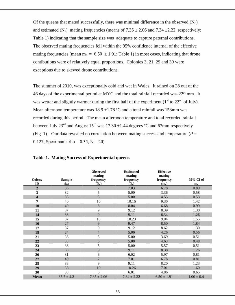
33
Of the queens that mated successfully, there was minimal difference in the observed (No)
and estimated (Ne) mating frequencies (means of 7.35 ± 2.06 and 7.34 ±2.22 respectively;
Table 1) indicating that the sample size was adequate to capture paternal contributions.
The observed mating frequencies fell within the 95% confidence internal of the effective
mating frequencies (mean me = 6.50 ± 1.91; Table 1) in most cases, indicating that drone
contibutions were of relatively equal proportions. Colonies 3, 21, 29 and 30 were
exceptions due to skewed drone contributions.
The summer of 2010, was exceptionally cold and wet in Wales. It rained on 28 out of the
46 days of the experimental period at MYC and the total rainfall recorded was 229 mm. It
was wetter and slightly warmer during the first half of the experiment (1st to 22
nd of July).
Mean afternoon temperature was 18.9 ±1.78 ºC and a total rainfall was 153mm was
recorded during this period. The mean afternoon temperature and total recorded rainfall
between July 23rd
and August 15th
was 17.30 ±1.44 degrees ºC and 67mm respectively
(Fig. 1). Our data revealed no correlation between mating success and temperature (P =
0.127, Spearman’s rho = 0.35, N = 20)
Table 1. Mating Success of Experimental queens
Colony
ID
Sample
size
Observed
mating
frequency
(N0)
Estimated
mating
frequency
(Ne)
Effective
mating
frequency
(me)
95% CI of
me
2 36 7 7.03 6.78 0.89
3 32 5 5.00 3.36 0.58
4 35 5 5.00 4.55 0.53
7 40 10 10.16 9.30 1.42
10 40 8 8.04 6.68 0.99
11 37 9 9.12 8.39 1.30
14 38 9 9.11 6.34 1.26
15 37 10 10.23 9.04 1.55
16 27 9 9.47 8.50 1.84
17 37 9 9.12 8.62 1.30
18 24 4 5.00 4.26 0.56
21 36 5 5.00 3.69 0.51
22 38 5 5.00 4.63 0.48
23 36 5 5.00 5.57 0.51
24 38 9 9.11 8.38 1.26
26 31 6 6.02 5.97 0.81
27 40 7 7.01 6.78 0.81
28 38 9 9.11 8.20 1.23
29 36 10 10.26 7.01 1.60
30 38 6 6.01 4.86 0.65
Mean 35.7 ± 4.2 7.35 ± 2.06 7.34 ± 2.22 6.50 ± 1.91 1.00 ± 0.4

34
The mating apiary (MYC) was located in a sheltered narrow valley. The mean wind speed
recorded at 15 m above the ground between the 24th
of July and the 12th
of August was
0.31 ± 0.39 ms-1
. The mean wind speed recorded at the DCA (approx. 7 m above ground)
during this same period was 1.85 ± 1.39 ms-1
. The DCA was in an open field and exposed
to the prevailing south easterly winds. Wind speeds were also generally higher during
periods of dry sunny weather. Queens mated when constant winds of 3.13 ms-1
were being
recorded at the DCA. Indeed, queens returned from mating flights when the DCA station
was consistently recording winds of between 3.39 and 3.80 ms-1
, and with gusts up to 5.28
ms-1
. No correlation was detected between mating success and wind-speed at either the
mating apiary (MYC) or the DCA (P = 0.369, and 0.366; Spearman’s rho = 0.22 and 0.31;
N = 19 and 11 respectively). The mean afternoon (1pm to 6pm) temperature at the mating
yard was 18.09 ± 1.84 ºC.
Figure 3. A figurative representation of queen mating flight times and duration in relation to wind
speeds (logged at 5 minutes intervals) recorded at the mating apiary (MYC) and at local drone
congregation area (DCA) between 12:00 and 17:00 hrs. on August 8th, 2010. Queen flight events
are represented by the horizontal lines. No correlation was detected between mating success and
wind speed at either the DCA or mating apiary.
Discussion
Our data suggest that both mating behaviour and success were affected by the weather.
Queens undertook many flights of short duration. Confirmed mating flights were far less
frequent and of significantly longer duration. Favourable mating opportunities were brief
and compressed by extended periods of rain and low temperatures. Of the twenty-eight
0.00
0.50
1.00
1.50
2.00
2.50
3.00
3.50
0:00:00 0:00:00 0:00:00 0:00:00 0:00:00
Win
d S
peed
(m
/s)
DCA WindSpeed
MYC WindSpeed
12:00 13:00 14:00 15:00 16:00 17:00
35
queens that were observed flying, three did not return, and five failed to successfully mate.
Our data detected no correlation between observed number of pairings (mating success)
and the average temperature and wind speeds recorded during the mating flight period. Of
the queens that successfully mated, 90% initiated oviposition after only one or two flights,
suggesting that they might have modulated their nuptial flight activity in response to
climatic conditions. A significant correlation was observed between mating success and
number of confirmed mating flights undertaken. Mating was also delayed in all cases, with
queens mating on average with seven drones (range 4-10). Similar mating frequencies
were obtained by Krause et al. [36] who suggested that environmental conditions had
limited the mating success (range 3-13) of A. m. carnica experimental queens. Similarly, it
was demonstrated that queens mated under island conditions have lower mating
frequencies than those mated on the European mainland [35, 37]. Bees considered well
adapted to northern climates (A.m. mellifera and A.m. carnica) will commonly mate with
15 or more drones when conditions allow [22].
Queens that undertook multiple mating flights were likely to have greater mating success.
It is not clear if queens ‘decide’ to undertake additional flights based on the copulation
success of previous flights. Tarpy and Page [32] observed no difference in the mating
success of queens that naturally started oviposition after one nuptial flight, and those that
attempted but were prevented from taking a second flight, and in which oviposition was
stimulated by CO2 anaesthesia. They concluded that queens have little behavioural control
over nuptial flight frequency. In contrast, Schlüns et al. [38] found a significant difference
in the mating success of similarly categorized experimental queens. They concluded that
queens can adjust their flight frequency based on the mating success of the previous flight,
and that number of copulations stimulates oviposition. They note that queens might have a
variable ‘threshold’ that is responsive to environmental queues. A lower threshold might
be expected during periods of poor weather due to the additional risk involved. Franck et
al. [39] also suggest that queens might adjust their mating flight frequency in accordance to
prevailing climatic conditions. Our observations support this postulate as queens took
numerous flights of short duration that were correlated with high humidity and low
temperature. Similar behaviour was described by Lensky and Demter [17] who noted that
queens took more flights of short duration during colder temperatures (15-20 ºC) and wind
speeds between 2.6 and 2.88 m/sec. We found no correlation between flight duration and
wind-speed, but queens mated successfully in constant winds up to 3.8 ms-1
. These
36
observations are also consistent with earlier research that suggests mating occurs only
when wind speeds are less than 4-5 m/s [17].
The mechanisms driving extreme polyandry in honeybees are not fully understood [36].
At the colony level, genetic variance hypotheses are favoured , although little increase in
intra-colony diversity occurs after six matings [22] suggesting minimal adaptive advantage
at higher mating numbers. Alternatively, the sperm limitation hypothesis proposes that
queens must mate multiply to offset premature sperm deficiency [14]. Woyke
demonstrated that the number of sperm stored in the spermatheca reaches capacity after
8µl of semen is inseminated. Work by Schlüns et al. [38] on sperm number and mating
frequency in naturally mated queens corroborated Woyke’s earlier instrumental
insemination work. It appears that naturally mated queens need only mate with 10 or so
drones to acquire a lifetime volume of sperm.
Based on research by Woyke [14], and Zmarlicki and Morse [15], delayed mating is
considered detrimental to queen vitality by beekeeping experts [9,10]. None of the
experimental queens in this study managed to mate within this optimal 14 day window.
The experimental period was characterized by long periods of cool overcast conditions,
including periods of extended daily rainfall (hence high humidity) (Fig. 1). The weather
clearly delayed mating, with queens not mating until they were 17 days old on average
(min 14 - max 23; note that this is an approximate age since actual date of emergence in
the mating nuclei was not known). Assuming time to oviposition was not delayed, our
queens would have started laying approximately six days later [10] at an average age of 23
days (range 17 -26 days), one week later than a recently reported species mean [10].
Previous research by Szabo et al. [40] and Skowronek et al. [41] had reported mean age of
oviposition as 10.6 and 10 days respectively, and the former suggest a relationship between
max daily temperature and time of oviposition. Guler and Alpay [12] reported a
significantly longer pre-ovipositon period for A. m. carnica (15.04 ± 0.23 days) compared
to five genotypes of A. m. liguistica and four regionally distinct groups of A. m. caucasica.
They found no significant loss in production due to delayed mating. Our data revealed no
correlation between approximate age of first mating, and ultimate mating success and we
cannot say whether delay in mating affected the ultimate mating success of our queens. It
is well known that instrumentally inseminated queens that are anesthetized by carbon

37
dioxide to stimulated egg-laying, take longer to start laying when compared to naturally
mated queens. No real difference in performance between these two groups is claimed [9].
Assessing the mated health of MYC queens
As previously noted, colony relatedness decays only minimally above a queen mating
frequency of six. Accordingly, fourteen of our twenty experimental colonies should
benefit from ‘adequate’ levels of intra-colony genetic variance. However, since the semen
from ten or so drones is required to fill a queen’s spermatheca to capacity with sperm, it
appears that approximately half of our mated queens may be inadequately mated and have
a shorter effective laying lifetime as a consequence. No diploid drone production by
experimental queens was noted. We observed solid brood patterns which suggested that
sufficient numbers of sex alleles were available in the population.
Summary
Our data suggest that queen flight behavior was influenced by environmental conditions
and that queens might modulate mating flights according to environmental cues.
Approximately twenty percent of our flying queens failed to mate, and most ‘successful’
queens undertook only one or two mating flights. Mean mating success was accordingly
low. It is possible that these results are normal for the area and reflect the fact that Wales
is on the fringe of the natural range of the western honeybee, and commonly experiences
high rainfall and cool temperatures due to its geographic location and elevated topography.
However, conditions during recent breeding seasons have been especially poor and the
observed results might be due to combined effects of location and medium to long-term
shifts in climate trends. We cannot rule out the possibility that one of the main causes of
premature failure of Welsh honeybee queens is suboptimal environmental conditions
during the breeding period and consequently inadequate mating.
Materials and Methods
Queen rearing and experimental set-up
The Cloake board queen rearing method was used during July and August 2010. Briefly,
this involved grafting one day old larvae into artificial queen cells and introducing them to
the top box of a two story colony. The queen and unsealed brood are isolated in the
bottom box and separated from the rest of the colony by a solid board (Cloake board). The
top box is supplied with pollen, nectar, and emerging brood and crowded with young nurse

38
bees. These manipulations are designed to mimic natural queen rearing conditions. Bees
in the top cell raising box experience overcrowding (which induces swarming tendencies)
and are missing a queen (which induces the colony to build emergency queen cells). Two
batches were raised in an effort to broaden the environmental variance, and to distribute
the observation/recording load. All experimental queens were grafted from the same
mother hive to limit genetic variance influencing mating success.
Each queen was allowed to emerge into a modified six-frame polystyrene nucleus hive
located at the experiment apiary in Maes-y-Coed (MYC), Ceredigion, Wales. These nuclei
incorporated a plexi-glass entrance tunnel gated at front and rear with a removable section
of queen excluder. The tunnels were designed to cover the hive entrances (approximate
dimension 5 cm x 3 cm) and were approximately 15 cm long, 12 cm wide, and 10 cm deep.
A queen exiting a hive was allowed access to the observation tunnel, but was prevented
from undergoing flight by a gate at the front end of the tunnel. When a queen was
observed in the tunnel, a rear gate was inserted to essentially cage the her. The front gate
was then removed to allow access to the open environment and possible flight. Departure
and return times were recorded. Returning queens would enter the entrance tunnel, and the
front gate would be closed. Access into the main hive body would still be restricted at this
point by the in-place rear gate. Return flights could then be confirmed, and queens could
be visually checked for signs of mating before being allowed access into the hive. The
first batch of queens were monitored between the 12th
and 26th
of July, and the second
batch between the 30th
of July and the 16th
of August. Daily monitoring occurred between
10:00 am 6:00 pm.
Queens utilize visual cues to orient onto their home nest entrance. To aid queen
orientation and to reduce the likelihood of drifting, colonies of differing colours were
paired and set side-by-side with entrances facing in opposite directions. Colony pairs (N =
7 per batch) were also spaced four to five feet apart and arranged into a square formation.
Queens were introduced as ripe (10 day old) cells, and emerged within a day or two into
the colony environment. The post-emergence period is the most critical time affecting
ultimate queen (and hence colony) success, and colonies are particularly sensitive to
disturbance during this time. Consequently, the experimental colonies were not disturbed
during this time, and queen were not individually marked.

39
Queens were allowed to take multiple flights. Flight time and duration were noted and
climatic conditions recorded using iROX PRO-X 2 weather stations. Weather data,
including temperature, rainfall, wind-speed and direction, were recorded every five
minutes during the experimental period.
A drone congregation area (DCA) just under 1km away from the mating yard was located
during this period. In contrast to the mating apiary, which was situated in a sheltered,
shaded valley, the DCA was located in a field up off the valley floor and was exposed to
all aspects of the prevailing weather. A second similar recording unit was therefore
installed at the local drone congregation area (DCA) before the August batch of queens
emerged.
Statistical Analyses of climate and mating success data
We investigated the influence of apiary temperature and wind speed on flight duration, and
tested the hypothesis that mating flights are significantly longer in duration than non-
mating localized flights. The temperature data were normally distributed but the
distribution of the flight duration data were visually skewed. They were therefore log
transformed and tested for normality using the Kolmogorov-Smirnov test.
We also tested for a correlation between mating success and number of putative mating
flights, apiary temperature, and wind speeds at both the mating apiary and DCA. The
mean temperatures and wind-speeds recorded during the flight periods (data logged every
5 mins.) were used in these instances. In addition, averages across number of flight were
used when queens had undertaken multiple mating flights. Non-parametric methods
(Spearman’s) was preferentially used to investigate possible effects on mating success due
to relatively low sample sizes. Sampling and genotyping experimental brood
Forty pupae per colony were sampled approximately six weeks after the queen cells were
introduced to eliminate the possibility of “phantom” genotypes drifting in with worker bees
from other colonies. Sealed brood was sampled at the purple- or post purple-eye stage and
individually stored in 100% ethanol. DNA was extracted from equal volumes of pupal leg
and thorax tissue using a modified version of the 96 well plate protocol described by
Lagisz et al. [42]. The extraction protocol was performed in 1.5ml tubes and the reagent
volumes adjusted accordingly. The extracted DNA was quantified using a NanoDrop
nd100 spectrophotometer and each sample was diluted to 50ng/µl for genotyping.
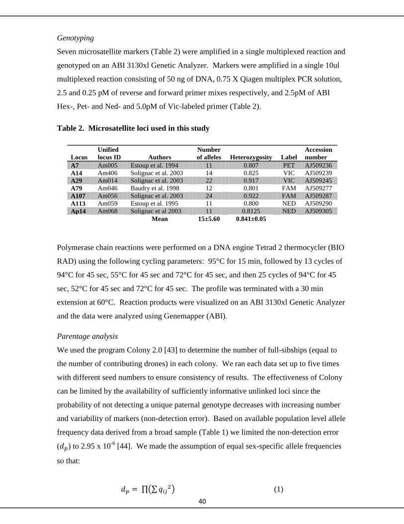
40
Genotyping
Seven microsatellite markers (Table 2) were amplified in a single multiplexed reaction and
genotyped on an ABI 3130xl Genetic Analyzer. Markers were amplified in a single 10ul
multiplexed reaction consisting of 50 ng of DNA, 0.75 X Qiagen multiplex PCR solution,
2.5 and 0.25 pM of reverse and forward primer mixes respectively, and 2.5pM of ABI
Hex-, Pet- and Ned- and 5.0pM of Vic-labeled primer (Table 2).
Table 2. Microsatellite loci used in this study
Locus
Unified
locus ID
Authors
Number
of alleles
Heterozygosity
Label
Accession
number
A7 Am005 Estoup et al. 1994 11 0.807 PET AJ509236
A14 Am406 Solignac et al. 2003 14 0.825 VIC AJ509239
A29 Am014 Solignac et al. 2003 22 0.917 VIC AJ509245
A79 Am046 Baudry et al. 1998 12 0.801 FAM AJ509277
A107 Am056 Solignac et al. 2003 24 0.922 FAM AJ509287
A113 Am059 Estoup et al. 1995 11 0.800 NED AJ509290
Ap14 Am068 Solignac et al 2003 11 0.8125 NED AJ509305 Mean 15±5.60 0.841±0.05
Polymerase chain reactions were performed on a DNA engine Tetrad 2 thermocycler (BIO
RAD) using the following cycling parameters: 95°C for 15 min, followed by 13 cycles of
94°C for 45 sec, 55°C for 45 sec and 72°C for 45 sec, and then 25 cycles of 94°C for 45
sec, 52°C for 45 sec and 72°C for 45 sec. The profile was terminated with a 30 min
extension at 60°C. Reaction products were visualized on an ABI 3130xl Genetic Analyzer
and the data were analyzed using Genemapper (ABI).
Parentage analysis
We used the program Colony 2.0 [43] to determine the number of full-sibships (equal to
the number of contributing drones) in each colony. We ran each data set up to five times
with different seed numbers to ensure consistency of results. The effectiveness of Colony
can be limited by the availability of sufficiently informative unlinked loci since the
probability of not detecting a unique paternal genotype decreases with increasing number
and variability of markers (non-detection error). Based on available population level allele
frequency data derived from a broad sample (Table 1) we limited the non-detection error
( ) to 2.95 x 10⁻⁶
[44]. We made the assumption of equal sex-specific allele frequencies
so that:
∏(∑ ) (1)

41
where is the frequency of allele i at locus j. Our markers provided sufficient power to
detect patrilines hence it is unlikely that discrepancies due to sex-specific allele frequency
differences would affect our results.
The observed number of patrilines (No) in a finite sample can underestimate the actual
number (Ne) due to non-sampling error. We calculated the estimated number of patrilines
(Ne) following procedure outlined by Schlüns et al. [38]:
[ ( ) ] (2)
where No = number of observed matings as determined by Colony, and n = the number of
colony progeny sampled. Ne = estimated number of matings and was determined by
iterating for (No). The degree of discrepancy between the observed and estimated
values provides an indication as to the adequacy of sampling. This calculation assumes
equal number of individuals per sub-family; an assumption that is unlikely to be true. We
therefore also present the 95% confidence interval around the effective paternity (me) as a
method to account for sampling error [25]. Effective paternity was calculated using an
unbiased estimator from Nielsen et al. [45] and provides a weighted value accounting for
disproportional paternal contributions
Acknowledgements
We thank David Wainwright of Tropical Forest Products for assistance during queen
rearing and setting up experimental hives. Paul Davison determined the location of the
drone congregation area and assisted setting up the weather monitoring station. Funding
was provided by the European Social Fund Convergence Program through a Knowledge
Economy Skills Scholarship (KESS), and by Tropical Forest Products.
Author Contributions
Conceived the experiment and wrote the paper: IW and AM. Performed the
experiment, collected the data and designed the microsatellite multiplex system IW.
Analyzed the data: IW
References
42
1. van Engelsdorp D, Meixner MD (2010) A historical review of managed honey bee
populations in Europe and the United States and the factors that may affect them. Journal
of Invertebrate Pathology 103 Suppl : S80–95.
2. Moritz RF , de Miranda J, Fries I, Le Conte Y, Neumann P, et al. (2010) Research
strategies to improve honeybee health in Europe. Apidologie 41: 227–242.
3. Le Conte Y, Brunet JL, McDonnell C, Dussaubat C, Alaux C (2011) Interactions
between risk factors in honey bees. In: Yoder JA , ed. Honey bee colony health
challenges and sustainable solutions. CRC Press. pp 215–222. Print ISBN: 978-1-4398-
7940-5 eBook ISBN: 978-1-4398-7941-2.
4. van Engelsdorp D, Hayes J, Underwood RM, Pettis J (2008) A survey of honey bee
colony losses in the U.S., fall 2007 to spring 2008. PloS ONE 3: e4071.
5. vanEngelsdorp D, Hayes Jr. J, Underwood RM, Caron D, Pettis J (2011) A survey of
managed honey bee colony losses in the USA, fall 2009 to winter 2010. Journal of
Apicultural Reseach 50: 1–10.
6. vanEngelsdorp D, Caron D, Hayes J, Underwood R, Henson M, et al. (2012) A
national survey of managed honey bee 2010-11 winter colony losses in the USA: results
from the bee informed partnership. Journal of Apicultural Reseach 51: 115–124.
7. Büchler R, Berg S, Le Conte Y (2010) Breeding for resistance to Varroa destructor in
Europe. Apidologie 41: 393–408.
8. Jensen AB, Palmer KA, Chaline N, Raine NE, Tofilski A, et al. (2005) Quantifying
honey bee mating range and isolation in semi-isolated valleys by DNA microsatellite
paternity analysis. Conservation Genetics 6: 527–537. doi:10.1007/s10592-005-9007-7.
9. Cobey SW (2007) Comparison studies of instrumentally inseminated and naturally
mated honey bee queens and factors affecting their performance. Apidologie 38: 390–410.
doi:10.1051/apido.
10. Mazeed A, Bienefeld K (2009) Does the duration of the pre oviposition period of
honeybee queens affect the honey production of colonies. Journal of Apicultural Science
53: 31–38.
11. Alaux C, Ducloz F, Crauser D, Le Conte Y (2010) Diet effects on honeybee
immunocompetence. Biology Letters 6: 562–565.
12. Guler A, Alpay H (2005) Reproductive character of some apis mellifera genotypes.
Journal of Animal and Veterinary Advances 4(10): 864-870.
13. Jones JC, Myerscough MR, Graham S, Oldroyd BP (2004) Honey bee nest
thermoregulation: diversity promotes stability. Science 305: 402–404.
14. Woyke J (1960) Natural and artificial insemination of queen honeybees. Pszczel. Zesz.
Nauk. 2(1) 4(3/4): 183-275 In Polish; English summary in Bee World 43(1): 21-25 (1962)
15. Zmarlicki C, and Morse R.A, (1962) The mating of aged virgin queen honeybees.
Journal of Apicultural Research 1: 62-63.
16. Fletcher DJC, Tribe GD (1977) Natural and emergency queen rearing by the African
bee A. m. adansonii and its relevance for successful queen production by beekeepers. In:
Fletcher DJC ed. African bees: taxonomy, biology and economic use, pp. 25–34. Pretoria:
Apimondia.
17. Lensky Y, Demter M (1985) Mating flights of the queen honeybee (Apis mellifera) in
a subtropical climate. Comparative Biochemistry and Physiology Part A: Physiology 81:
229–241.
18. Woyke J, Mmajewska B, Samborski J, Bratkowski J, Jojczyk A (2008) Onset of
oviposition by honey bee queens, mated either naturally or by various instrumental
insemination methods, fits a lognormal distribution. Journal of Apicultural Research 47:
1–9.
43
19. Patricio K, Cruz-Landim C (2002) Mating influence in the ovary differentiation in
adult queens of Apis mellifera L. Brazilian Journal of Biology 62(4A): 641-649.
20. Cruz-landim C, Patrício K, Fernando W, Antonialli WF (2006) Cell death and
ovarian development in highly eusocial bees (Hymenoptera, Apidae): caste differentiation
and worker egg laying. Brazilian Journal of Morphological Sciences 23(1): 27-42.
21. Tarpy DR, Keller JJ, Caren JR, Delaney DA (2012) Assessing the mating “ health ” of
commercial honey bee queens. Journal of Economic Entomology 105(1): 20-25.
doi.org/10.1603/EC11276.
22. Palmer KA, Oldroyd BP (2001) Review article Evolution of multiple mating in the
genus Apis. Apidologie 31: 235–248.
23. Tarpy DR, Nielsen R, Nielsen DI (2004) A scientific note on the revised estimates of
effective paternity frequency in Apis. Insectes Sociaux 51: 203–204.
24. Kraus FB, Neumann P, Moritz RF. (2005) Genetic variance of mating frequency in the
honeybee (Apis mellifera L.). Insectes Sociaux 52: 1–5.
25. Tarpy DR, Nielsen D (2002) Sampling error, effective paternity, and estimating the
genetic structure of honey bee colonies (Hymenoptera: Apidae ). Annals of the
Entomological Society of America 95(4): 513-528.
26. Richard FJ, Tarpy DR, Grozinger CM (2007) Effects of insemination quantity on
honey bee queen physiology. PLoS ONE 2(10): e980. doi:10.1371/journal.pone.0000980 .
27. Tarpy DR (2003) Genetic diversity within honeybee colonies prevents severe
infections and promotes colony growth. Proceeding of the Royal Society of London Series
B-Biological Sciences 270: 99-103.
28. Seeley TD, Tarpy DR (2007) Queen promiscuity lowers disease within honeybee
colonies. Proceedings of the Royal Society B 274: 67–72.
29. Invernizzi C, Peñagaricano F, Tomasco IH (2009) Intracolonial genetic variability in
honeybee larval resistance to the chalkbrood and American foulbrood parasites. Insectes
Sociaux 56: 233–240.
30. Tarpy DR, Page RE (2001) The curious promiscuity of queen honey bees (Apis
mellifera): Evolutionary and Behavioral Mechanisms: Annales Zoologici Fennici 38: 255–
265.
31. Page RE, Marks RW (1982) The population genetics of sex determination in honey
bees: random mating in closed populations. Heredity 48: 263–270.
32. Tarpy D, Page RE (2000) No behavioral control over mating frequency in queen
honey bees (Apis mellifera L.): Implications for the evolution of extreme polyandry.
American Naturalist 155: 820–827.
33. Beye M, Hasselmann M, Fondrk MK, Page RE, Omholt SW (2003) The gene csd is
the primary signal for sexual development in the honeybee and encodes an SR-type
protein. Cell 114: 419–429.
34. Neumann P, vanPraagh JP, Moritzux RFA, Dustmann JH (1999) Testing reliability of
a potential island mating apiary using DNA microsatellites. Apidologie 30: 257-276.
35. Cobey S (2005) A versatile queen rearing and banking system Part 1: the Cloake
board method of queen rearing. American Bee Journal 4:308-311.
36. Kraus FB, Neumann P, van Praagh J, Moritz RF (2004) Sperm limitation and the
evolution of extreme polyandry in honeybees (Apis mellifera L.). Behavioral Ecology and
Sociobiology 55: 494–501.
37. Scharpenberg H, Neumann P, Praagh JP Van, Moritz RFA (2006) Reliability of an
island mating apiary under routine management. Journal of Apicultural Research 45: 153–
154.

44
38. Schlüns H, Moritz RF, Neumann P, Kryger P, Koeniger G (2005) Multiple nuptial
flights, sperm transfer, and the evolution of extreme polyandry in honeybee queens.
Animal Behaviour 70: 125–131.
39. Franck P, Koeniger N, Lahner G, Crewe RM, Solignac M (2006) Evolution of extreme
polyandry: an estimate of mating frequency in two African honeybee subspecies, Apis
mellifera monticola and A .m. scutellata. Insectes Sociaux 47(4): 364-370.
doi:10.1007/PL00001732.
40. Szabo TJ, Mills PF, Heikel DT (1987) Effects of honeybee queen weight and air
temperature on the initiation of oviposition. Journal of Apicultural Research 26: 73-78.
41. Skowronek W, Kruk C, Klopot J (2002) Factors affecting oviposition of artificially
inseminated honeybee queens. Journal of Apicultural Science 46(4): 85-89.
42. Lagisz M, Port G, Wolff K (2010) A cost-effective, simple and high-throughput
method for DNA extraction from insects. Insect Science: 465–470.
43. Jones OR, Wang J (2010) COLONY: a program for parentage and sibship inference
from multilocus genotype data. Molecular Ecology Resources 10: 551–555.
44. Boomsma JJ, Ratnieks (1996) Paternity in eusocial hymenoptera. Philosophical
Transactions of the Royal Society of London B. 351:947-975.
45. Nielsen R, Tarpy DR, Reeve HK (2003) Estimating effective paternity number in
social insects and the effective number of alleles in a population. Molecular Ecology 12:
3157–3164
45
Chapter 3
Selection on Phenotype
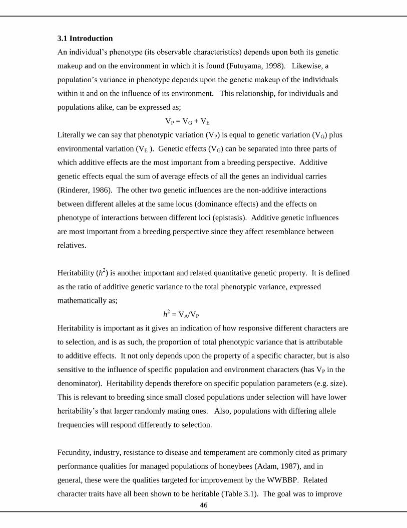
46
3.1 Introduction
An individual’s phenotype (its observable characteristics) depends upon both its genetic
makeup and on the environment in which it is found (Futuyama, 1998). Likewise, a
population’s variance in phenotype depends upon the genetic makeup of the individuals
within it and on the influence of its environment. This relationship, for individuals and
populations alike, can be expressed as;
VP = VG + VE
Literally we can say that phenotypic variation (VP) is equal to genetic variation (VG) plus
environmental variation (VE ). Genetic effects (VG) can be separated into three parts of
which additive effects are the most important from a breeding perspective. Additive
genetic effects equal the sum of average effects of all the genes an individual carries
(Rinderer, 1986). The other two genetic influences are the non-additive interactions
between different alleles at the same locus (dominance effects) and the effects on
phenotype of interactions between different loci (epistasis). Additive genetic influences
are most important from a breeding perspective since they affect resemblance between
relatives.
Heritability (h2) is another important and related quantitative genetic property. It is defined
as the ratio of additive genetic variance to the total phenotypic variance, expressed
mathematically as;
h2 = VA/VP
Heritability is important as it gives an indication of how responsive different characters are
to selection, and is as such, the proportion of total phenotypic variance that is attributable
to additive effects. It not only depends upon the property of a specific character, but is also
sensitive to the influence of specific population and environment characters (has VP in the
denominator). Heritability depends therefore on specific population parameters (e.g. size).
This is relevant to breeding since small closed populations under selection will have lower
heritability’s that larger randomly mating ones. Also, populations with differing allele
frequencies will respond differently to selection.
Fecundity, industry, resistance to disease and temperament are commonly cited as primary
performance qualities for managed populations of honeybees (Adam, 1987), and in
general, these were the qualities targeted for improvement by the WWBBP. Related
character traits have all been shown to be heritable (Table 3.1). The goal was to improve
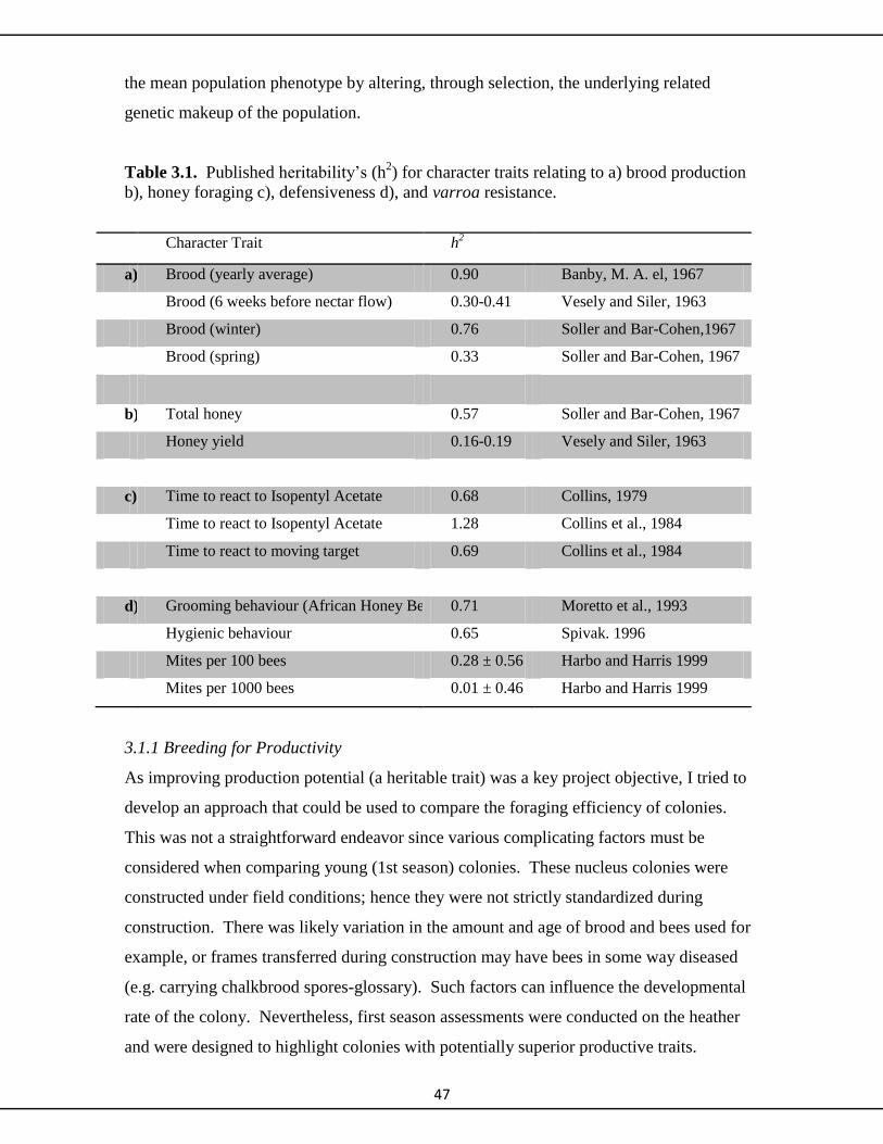
47
the mean population phenotype by altering, through selection, the underlying related
genetic makeup of the population.
Table 3.1. Published heritability’s (h2) for character traits relating to a) brood production
b), honey foraging c), defensiveness d), and varroa resistance.
Character Trait h2
a) Brood (yearly average) 0.90 Banby, M. A. el, 1967
Brood (6 weeks before nectar flow) 0.30-0.41 Vesely and Siler, 1963
Brood (winter) 0.76 Soller and Bar-Cohen,1967
Brood (spring) 0.33 Soller and Bar-Cohen, 1967
b) Total honey 0.57 Soller and Bar-Cohen, 1967
Honey yield 0.16-0.19 Vesely and Siler, 1963
c) Time to react to Isopentyl Acetate 0.68 Collins, 1979
Time to react to Isopentyl Acetate 1.28 Collins et al., 1984
Time to react to moving target 0.69 Collins et al., 1984
d) Grooming behaviour (African Honey Bee) 0.71 Moretto et al., 1993
Hygienic behaviour 0.65 Spivak. 1996
Mites per 100 bees 0.28 ± 0.56 Harbo and Harris 1999
Mites per 1000 bees 0.01 ± 0.46 Harbo and Harris 1999
3.1.1 Breeding for Productivity
As improving production potential (a heritable trait) was a key project objective, I tried to
develop an approach that could be used to compare the foraging efficiency of colonies.
This was not a straightforward endeavor since various complicating factors must be
considered when comparing young (1st season) colonies. These nucleus colonies were
constructed under field conditions; hence they were not strictly standardized during
construction. There was likely variation in the amount and age of brood and bees used for
example, or frames transferred during construction may have bees in some way diseased
(e.g. carrying chalkbrood spores-glossary). Such factors can influence the developmental
rate of the colony. Nevertheless, first season assessments were conducted on the heather
and were designed to highlight colonies with potentially superior productive traits.
48
I considered comparing colonies for production potential as follows. It seems
hypothetically possible (assuming all other contributing factors to be equal) that a colony
with fewer but more efficient foraging bees might weigh more than a colony with greater
numbers of less industrious bees (i.e., less efficient at gathering nectar and pollen). One
might therefore observe a lack of correlation between colony strength and weight change
during a nectar flow if a population has high variance in foraging efficiency. By recording
weight change, one can eliminate confounding factors such as unequal weight of colony
woodenware. Another possible way to identify better producing colonies might be to
regress the end of season colony weight on frames of bees. If a correlation is observed (as
might be expected) between these two variables, an expected curve can be generated.
Colonies with above average weight, in relation to number of bees (i.e. above the curve)
would be highlighted as better performing.
3.1.2 Selecting for varroa mite resistance
A conscious decision was made not to select for specific heritable mite resistant/tolerant
behaviors (e.g. hygienic behaviour, varroa sensitive hygiene VSH, grooming). Bee strains
with enhanced VSH qualities have been developed by federally funded establishments in
the USA, but such work is too demanding of time and effort (selecting for VSH
particularly so) for small scale operations. There is also a cost incurred by focusing only
on a single resistance specific trait. Overly vigorous VSH colonies can retard brood
development and have reduced production potential, and may make them more susceptible
to cold weather, for example. Since so much goes unnoticed in the honeybee colony, it is
likely that many subtle and currently unrecognized mechanisms confer varying degrees of
colony level tolerance. Independent bee operation can enhance these population traits by
each year breeding only with the strongest treatment free survivors.
3.1.3. Other considerations relevant to honeybees
The eusocial structure of the honeybee colony complicates the process of selection and
breeding. For example, for certain traits (e.g. honey production) we are assessing the
performance of an individual (queen) for breeding based on the performance and behavior
of a collective group from a different caste (the workers). Although queens and workers
that are raised in the same colony are genetically similar, they develop in different
environments. Similarly, we may select drone- producing colonies based on the hygienic
49
performance of the worker population. In addition, the relatedness of individuals within a
colony varies to a greater or lesser extend depending on the number of contributing
patrilines. Without artificially inseminating queens (Instrumental Insemination) one can
never therefore be certain of the paternal source when selecting queens.
Wales is on the north-western margin of the native distribution of the honeybee; hence
consideration was given during breeder selection to regionally-appropriate characteristics.
For example, the queen must be sensitive to environmental cues to control brood rearing
since the region can experience prolonged periods of inclement weather at any-time of the
year. Colonies must be able to rapidly expand and forage efficiently during periods of
good weather, and display frugality during periods of dearth. The strongest of surviving
overwintered colonies were compared in the spring 2011. Potential breeders were assessed
by comparing colony condition (strength and general health) and general organization of
the brood nest. Choice colonies had nests comprising of ample sealed and unsealed brood
surrounded by consecutive arches of pollen and nectar/honey respectively.
Apiary location can also greatly influence colony performance. Factors such as elevation,
aspect, shelter and availability of forage will all affect colony performance. Breeders were
therefore selected from different overwintering locations in an effort to accommodate for
differences due to environmental influences. The breeder daughter (test) colonies were
similarly distributed to compare the performance of sister queens in different environments.
Wales has recently experienced a series of poor summers, and accounting for confounding
environmental effects on monitored traits was expected to be challenging in an applied
setting. I nevertheless expected some observable change due to selection in the population
during the experimental period. In particular, I expected greater uniformity as the number
of breeders was effectively dropped from 8 to 4 between years. That is, as genetic input
was constrained across generations, I hypothesized a detectable and concurrent reduction in
colony level phenotypic variance. Of the characteristics I monitored, colony strength and
temperament were considered to be more likely to adaptively respond to selection. Mite
counts per colony is not a strongly heritable trait, and detectable reductions in population
level variance was considered less likely.
3.2 Methods

50
3.2.1 Grafting and raising queen cells
Frames with brood of appropriate age were removed from selected breeders, and marked
with coloured press-pins in the field. These were placed in nuc-boxes (with bees to help
maintain brooding environment) for transportation back to the grafting shed.
A variation on the Cloake board method was used for queen rearing. A single cell raising
unit consisted of two stacked Modified Dadant (MD) brood boxes. Strong colonies were
used as raisers since high bee density (particularly young nurse bees) is needed. The
colony queen was isolated in the bottom box along with unsealed brood, stores and empty
frames. The remaining brood, stores and empty drawn comb were placed in the top box
which was separated from the one below by a queen excluder (glossary). A single entrance
located at the front of the bottom box is provided at this stage. Each cell raiser was
copiously fed with syrup and pollen, particularly in the absence of strong natural nectar
flows, and left for up to eight days in preparation for receiving grafts. By then, many
young nurse bees would have emerged in the top box and any remaining brood in this part
of the hive would be sealed.
In preparing the colony to accept grafted larvae, all the top box frames were shaken of bees
and checked for natural queen cells. It is vital that no queens (virgin or mature) or queen
cells be present in the cell raising box (top box in our method). Any suspicious queen cell
structures were removed. I also ensured that the colony queen was still in the bottom box
and had not accidently passed into the top. The bottom box and entrance was then turned
through 180°, and a solid board (the Cloake board) was placed on top before the top box
was replaced. A solid board now separated the two colony halves, isolating the bees above
from the effects of the queen down below. The board also provides a new front entrance
into the top portion of the hive only. Conditioned front oriented bees leaving the hive via
the rear bottom box entrance would then return into the top. These manipulations
increased bee density in the top box in preparation for cell building.
Theoretical modelling by Moritz (1984) suggested that inbreeding could be limited to
acceptable levels for 10 generations if a minimum of 8 breeder queens per year were used.
Eleven breeders were therefore selected in the spring of 2011 from a source population
consisting of 2010 and older colonies (Table 3.1a). The breeding program logistics proved
challenging with this number of breeders. In addition, some breeders were not well
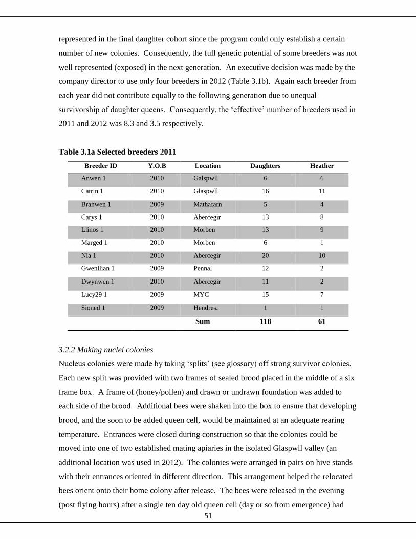
51
represented in the final daughter cohort since the program could only establish a certain
number of new colonies. Consequently, the full genetic potential of some breeders was not
well represented (exposed) in the next generation. An executive decision was made by the
company director to use only four breeders in 2012 (Table 3.1b). Again each breeder from
each year did not contribute equally to the following generation due to unequal
survivorship of daughter queens. Consequently, the ‘effective’ number of breeders used in
2011 and 2012 was 8.3 and 3.5 respectively.
Table 3.1a Selected breeders 2011
Breeder ID Y.O.B Location Daughters Heather
Anwen 1 2010 Galspwll 6 6
Catrin 1 2010 Glaspwll 16 11
Branwen 1 2009 Mathafarn 5 4
Carys 1 2010 Abercegir 13 8
Llinos 1 2010 Morben 13 9
Marged 1 2010 Morben 6 1
Nia 1 2010 Abercegir 20 10
Gwenllian 1 2009 Pennal 12 2
Dwynwen 1 2010 Abercegir 11 2
Lucy29 1 2009 MYC 15 7
Sioned 1 2009 Hendres. 1 1
Sum 118 61
3.2.2 Making nuclei colonies
Nucleus colonies were made by taking ‘splits’ (see glossary) off strong survivor colonies.
Each new split was provided with two frames of sealed brood placed in the middle of a six
frame box. A frame of (honey/pollen) and drawn or undrawn foundation was added to
each side of the brood. Additional bees were shaken into the box to ensure that developing
brood, and the soon to be added queen cell, would be maintained at an adequate rearing
temperature. Entrances were closed during construction so that the colonies could be
moved into one of two established mating apiaries in the isolated Glaspwll valley (an
additional location was used in 2012). The colonies were arranged in pairs on hive stands
with their entrances oriented in different direction. This arrangement helped the relocated
bees orient onto their home colony after release. The bees were released in the evening
(post flying hours) after a single ten day old queen cell (day or so from emergence) had
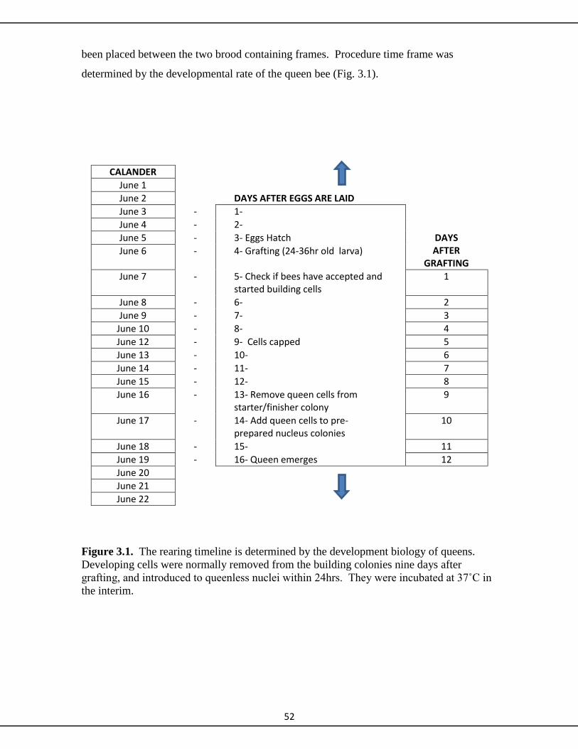
52
been placed between the two brood containing frames. Procedure time frame was
determined by the developmental rate of the queen bee (Fig. 3.1).
CALANDER
June 1
June 2 DAYS AFTER EGGS ARE LAID
June 3 - 1-
June 4 - 2-
June 5 - 3- Eggs Hatch DAYS AFTER
GRAFTING June 6 - 4- Grafting (24-36hr old larva)
June 7 - 5- Check if bees have accepted and started building cells
1
June 8 - 6- 2
June 9 - 7- 3
June 10 - 8- 4
June 12 - 9- Cells capped 5
June 13 - 10- 6
June 14 - 11- 7
June 15 - 12- 8
June 16 - 13- Remove queen cells from starter/finisher colony
9
June 17 - 14- Add queen cells to pre-prepared nucleus colonies
10
June 18 - 15- 11
June 19 - 16- Queen emerges 12
June 20
June 21
June 22
Figure 3.1. The rearing timeline is determined by the development biology of queens.
Developing cells were normally removed from the building colonies nine days after
grafting, and introduced to queenless nuclei within 24hrs. They were incubated at 37˚C in
the interim.

53
Table 3.1b Selected breeders 2012
Breeder Y.O.B Daughters
Anwen 2 2011 10
Carys 2 2011 21
Catrin 2 2011 9
Llinos 2 2011 18
Sum 58
The nucleus colonies were left undisturbed for a month to give successfully mated queens
time to mature and start egg-laying. Colonies are sensitive during this period since the
post-emergent queens have entered the most precarious developmental phase. They have
only a brief window to successfully mate, and they must leave the safety of the hive to do
so. Mating on the wing they must navigate through unfamiliar territory and possibly brave
poor weather and predation to do so.
3.2.3 Measuring colony strength and foraging efficiency
Various measurements gave an indication of colony strength. Individual frames were
visually inspected during colony development and scored for brood strength (Fig 3.2).
Each side of a brood bearing frame was scored for brood density (range 1-4) so that a
whole frame could receive a maximum score of 8. Individual frame scores were tallied for
an overall colony score. The ‘frames with bees’ index was a simple description of how
many frames the bees were actively occupying and utilizing. A homemade portable scale
was used to weigh single box hives in the field (Fig. 3.3).
Comparative weight gains during periods of nectar flow were used in an effort to identify
colonies with foraging with above average efficiency. Colonies were weighed before and
after periods of good weather while on the heather, and measurements were taken in the
evening when most of the flying bees were back in the hive. The goal was to assess
foraging efficiency by comparing colony strength to rate of weight gain during nectar
flows. Weather conditions on the heather moors were uncharacteristically poor during the
2012 season. Weight gain comparisons were not possible this season since the bees were
not able to forage for suitably prolonged periods. Heather quality was low and colonies
weight began dropping towards the end of the season.
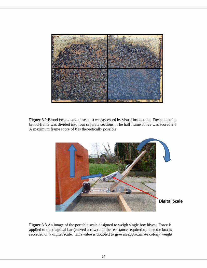
54
Digital Scale
Figure 3.2 Brood (sealed and unsealed) was assessed by visual inspection. Each side of a
brood-frame was divided into four separate sections. The half frame above was scored 2.5.
A maximum frame score of 8 is theoretically possible
Figure 3.3 An image of the portable scale designed to weigh single box hives. Force is
applied to the diagonal bar (curved arrow) and the resistance required to raise the box is
recorded on a digital scale. This value is doubled to give an approximate colony weight.

55
3.2.4 Varroa mite counts
The sugar shake method (Macedo and Ellis 2002) was used to monitor for varroa.
Approximately 300 bees (approx. 150ml marked on clear jar) were shaken off a frame of
brood (after ensuring that the colony queen was elsewhere) and placed into a jar covered
with a woven wire 8 mesh cover lid. Using a hive tool tip, approximately one table-spoon
of dry powdered sugar was added, and the jar left for one minute. The jar was then shaken
vigorously over a white enamel bowl containing water. The dark dislodged varroa would
be visible floating on the water against the light background.
3.2.5 Measuring colony temperament
Temperament was assessed subjectively in 2011, and quantitatively in 2012. Colonies
were subjectively given a score (range 1—5) based on behavior. Particularly defensive
(i.e., quick to begin stinging) and ‘runny’ colonies were scored the lowest, and docile calm
colonies the highest. A more quantitative method was adopted in 2012 because the bees
were defensive from the beginning of the season. Although environmental conditions were
particularly bad this season (possibly a significant contributing factor) there was concern
that genetic influences due to breeding were affecting population temperament. Colony
temperament was investigated using similar methods to those described by Guzman-Novoa
et al. (2004). Immediately after opening the hive, a piece of black leather (5cm square)
that was stapled to the end of a wooden wand was lowered to within approximately 10cm
of the frames. The leather antagonist was rhythmically lowered and raised once a second
for 45 seconds. The number of stingers in the leather was used as a quantitative
assessment of colony defensiveness. The temperament of all the experimental daughters
were qualitatively assessed as described above after the colonies had matured and migrated
to the heather. All colonies were tested on the same day and under similar weather
conditions. A control apiary comprising of 2011 and older colonies from an unknown mix
of breeders (N=26), representing the unselected background phenotype was also tested a
few days later under similar weather conditions.
3.2.6 Data analysis and colony comparisons
A z-score index was used to compare colonies of different age (n = 3) classes in 2011, and
a similar approach was used to compare the daughter colonies of different breeders (n = 2)
in 2012. Z-scores allow comparison among cohorts in units of standard deviations where:
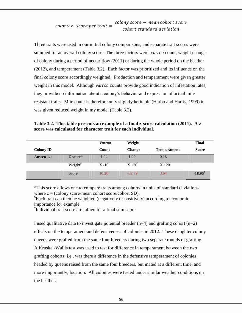
56
Three traits were used in our initial colony comparisons, and separate trait scores were
summed for an overall colony score. The three factors were: varroa count, weight change
of colony during a period of nectar flow (2011) or during the whole period on the heather
(2012), and temperament (Table 3.2). Each factor was prioritized and its influence on the
final colony score accordingly weighted. Production and temperament were given greater
weight in this model. Although varroa counts provide good indication of infestation rates,
they provide no information about a colony’s behavior and expression of actual mite
resistant traits. Mite count is therefore only slightly heritable (Harbo and Harris, 1999) it
was given reduced weight in my model (Table 3.2).
Table 3.2. This table presents an example of a final z-score calculation (2011). A z-
score was calculated for character trait for each individual.
Colony ID
Varroa
Count
Weight
Change
Temperament
Final
Score
Anwen 1.1 Z-score* -1.02 -1.09 0.18
Weight$
X -10 X +30 X +20
Score 10.20 -32.79 3.64 -18.96#
*This score allows one to compare traits among cohorts in units of standard deviations
where z = (colony score-mean cohort score/cohort SD). $Each trait can then be weighted (negatively or positively) according to economic
importance for example. *Individual trait score are tallied for a final sum score
I used qualitative data to investigate potential breeder (n=4) and grafting cohort (n=2)
effects on the temperament and defensiveness of colonies in 2012. These daughter colony
queens were grafted from the same four breeders during two separate rounds of grafting.
A Kruskal-Wallis test was used to test for difference in temperament between the two
grafting cohorts; i.e., was there a difference in the defensive temperament of colonies
headed by queens raised from the same four breeders, but mated at a different time, and
more importantly, location. All colonies were tested under similar weather conditions on
the heather.

57
Preliminary assessments, standardizing for colony age (2011) and breeder (2012) using z-
scores, identified the thirty top performing hives each year. These were moved into two
overwintering apiaries in mid-Wales for possible selection as breeders the following year.
Accumulated colony specific data were forwarded to the commercial partner.
3.2.7 A comment on monitoring adaptive change
The WWBBP is a long term project aiming to improve the resilience and production
potential of its bee stock. The program is in the early stages, having currently gone
through two rounds of breeding. It is a field operation exposed to the vagaries of the
weather. Environmental conditions have been uncharacteristically demanding during
recent years, and demonstrable evidence that selection is having a positive effect on
desired character traits is lacking. A limitation of this field approach is the lack of suitable
control populations, to which adaptive shifts in the test group could be compared. In order
to demonstrate an effect due to selection, I compare trait variances across generations,
under the assumption that it should shrink due to greater genetic uniformity resulting from
selection.
A total of 118 new colonies were established in the spring of 2011 (Table 3.1a) and
approximately seventy-five percent mating success was achieved. The most promising
looking colonies (N = 61; based on colony strength and condition at time of transfer from
nucleus boxes into full bodied hives) were selected for a 60 mile migration to the heather
moors during the first 2 weeks of August. Each of the three age classes was represented by
21, 28 and 12 colonies respectively.
3.3 Results
3.3.1 Season 2011
Good weather between 23rd
and the 29th
of August allowed bees to forage on the heather.
An average weight gain of 3.04 ± 1.96 kg was recorded and attributed to accumulation of
stores (Figure 3.4).

58
Figure. 3.4 shows changes in hive weights recorded between the 23rd and 29th of August,
2011. Colonies are grouped into breeder daughter cohorts. The error bars indicate one
standard deviation of scale precision. This was determined after conducting multiple trials
using the scale on a known weight.
The mean number of varroa counted, and frames of bees per colony on 1st of October, was
4.90 ± 7.22 and 6.29 ± 1.49 respectively. There was no correlation between weight change
during the nectar flow that occurred between the 23rd
and 29th
of August and colony size at
end of season (frames of bees on 1st of October; F= 0.47, = 0.11, P = 0.49), but there
was a highly significant correlation between colony weight and frames of bees on the 30th
of September (P<0.001; = 0.25; Fig 3.5). There was also a significant correlation
between weight change during the nectar flow and weight of colony approximately one
month later (P < 0.001, R^2= 0.36). The top 30 colonies were highlighted using a z-score
index that accounted for difference in development age (Table 3.3).

59
Figure 3.5 The regression of colony weight on frames of bees (colony size) using data collected on
the 30th of September and the 1
st of October 2011 respectively. Colonies above the linear curve (as
predicted by the displayed regression equation) are heavier in relation to the number of bees
present, suggesting that bees from these colonies displayed greater foraging efficiency . These
better performing colonies are highlighted in Table 3.3, which outlines the top 30 colonies
determined using a z-score index.
3.3.2 2012 Season
All successfully mated colonies (N=58) were taken to the heather in 2012. Heather
development was delayed due to poor weather and there were no prolonged periods of
nectar flow suitable for assessing foraging efficiency. Colonies gained a mean of 2.14 ±
1.81 kg between the 8th
and 26th
of August, and a mean of 0.87 ± 3.8 kg between 26th
of
August and the 6th
of September. A mean weight change of -0.77 ± 1.31 kg was recorded
between the 6th
and the 9th
of September.
Colonies were monitored for varroa, number of frames with bees, and brood coverage,
between 28th
August and 9th
of September. The mean number of varroa, and frames of
bees counted per colony was 12.18 ± 11.02 and 6.61 ± 0.94 respectively. There was a
significant negative correlation between the change in hive weight that occurred between
the 6th
and 9th
of September, and frames of bees and amount of brood recorded during the
monitoring period ( = -0.19 and -0.36, and P = 0.024 and 0.006 respectively). There was
no significant correlation between colony weight on the 8th
of September and colony size
(frames of bees and brood score; P = 0.09 and 0.09, and = 0.26 and 0.25 respectively).
y = 1.02x + 22.16 R² = 0.25
0
5
10
15
20
25
30
35
40
0 2 4 6 8 10 12
Hiv
e W
eig
ht
Frames of Bees
Hive Weight
Linear (Hive Weight)

60
Neither was there a significant correlation between weight change and weight of colony
one month later (P = 0.46, = 0.1). The top 30 colonies were highlighted using z-score
index to account for some difference in breeder group (Table 3.4).
Table 3.3. Table of 2011 daughters in order of performance on z-score analysis
*Indicates individuals that were above trend line predicted by the regression equation
(Figure 3.5)
**Rejected by z-score analysis due to bad temperament
*** Was above trend line but colony heavily infested with mites
Putative Breeders For Production
Queen ID Score Queen ID Score
Catrin 1.7 76.61 Anwen 1.6 -4.47
Carys 1.6 45.87 Anwen 1.5 -5.29
Carys 1.5 41.59 Llinos 1.11 -6.75
Catrin 1.3 38.41 Llinos 1.5 -8.90
Catrin 1.9* 31.82 Anwen 1.1 -9.17
Carys 1.3* 30.90 Branwen 1.1 -9.51
Catrin 1.4* 29.59 Anwen 1.4 -11.18
Anwen 1.2* 29.42 Catrin 1.15 -13.77
Lucy29 1.13* 29.18 Lucy29 1.8 -14.33
Marged 1.6 28.72 Nia 1.18** -15.34
Llinos 1.6 24.30 Nia 1.15 -17.88
Llinos 1.2 24.18 Carys 1.12 -19.54
Lucy29 1.3* 21.52 Branwen 1.3 -20.04
Carys 1.11 17.81 Dwynwen 1.9 -22.33
Lucy29 1.1 15.57 Nia 1.5 -23.12
Catrin 1.5* 15.01 Gwenllian 1.8 -23.31
Catrin 1.8 12.84 Nia 1.14 -25.41
Catrin 1.16 12.60 Lucy29 1.9 -25.92
Carys 1.13* 12.49 Llinos 1.3 -28.02
Anwen 1.3 8.88 Llinos 1.10 -28.44
Sioned 1.1* 5.83 Dwynwen 1.6 -30.44
Llinos 1.12* 5.63 Nia 1.1 -32.31
Catrin 1.6* 0.88 Llinos 1.1 -34.91
Catrin 1.11 -0.45 Nia 1.12 -35.13
Carys 1.10 -0.55 Nia 1.3 -39.73
Lucy29 1.6* -0.64 Nia 1.13 -46.54
Llinos 1.7 -0.82 Carys 1.4 -52.31
Catrin 1.10 -1.54 Lucy29 1.2*** -56.19
Branwen 1.4* -2.82 Nia 1.20 -56.43
Branwen 1.5 -3.64 Nia 1.17 -142.10
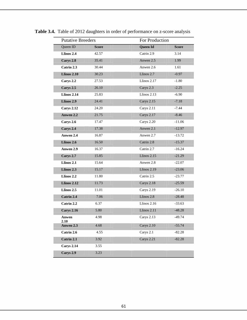
61
Table 3.4. Table of 2012 daughters in order of performance on z-score analysis
Putative Breeders For Production
Queen ID Score Queen Id Score
Llinos 2.4 42.57 Catrin 2.9 3.14
Carys 2.8 35.41 Anwen 2.5 1.99
Catrin 2.3 30.44 Anwen 2.6 1.61
Llinos 2.10 30.23 Llinos 2.7 -0.97
Carys 2.2 27.53 Llinos 2.17 -1.80
Carys 2.5 26.10 Carys 2.3 -2.25
Llinos 2.14 25.83 Llinos 2.13 -6.90
Llinos 2.9 24.41 Carys 2.15 -7.18
Carys 2.12 24.20 Carys 2.11 -7.44
Anwen 2.2 21.75 Carys 2.17 -8.46
Carys 2.6 17.47 Carys 2.20 -11.06
Carys 2.4 17.38 Anwen 2.1 -12.97
Anwen 2.4 16.87 Anwen 2.7 -13.72
Llinos 2.6 16.50 Catrin 2.8 -15.37
Anwen 2.9 16.37 Catrin 2.7 -16.24
Carys 2.7 15.85 Llinos 2.15 -21.29
Llinos 2.1 15.64 Anwen 2.8 -22.07
Llinos 2.3 15.17 Llinos 2.19 -23.06
Llinos 2.2 11.80 Catrin 2.5 -23.77
Llinos 2.12 11.73 Carys 2.18 -25.59
Llinos 2.5 11.01 Carys 2.19 -26.10
Catrin 2.4 7.06 Llinos 2.8 -28.48
Catrin 2.2 6.37 Llinos 2.16 -33.63
Carys 2.16 5.80 Llinos 2.11 -48.28
Anwen
2.10
4.98 Carys 2.13 -49.74
Anwen 2.3 4.68 Carys 2.10 -55.74
Catrin 2.6 4.55 Carys 2.1 -82.28
Catrin 2.1 3.92 Carys 2.21 -82.28
Carys 2.14 3.55
Carys 2.9 3.23
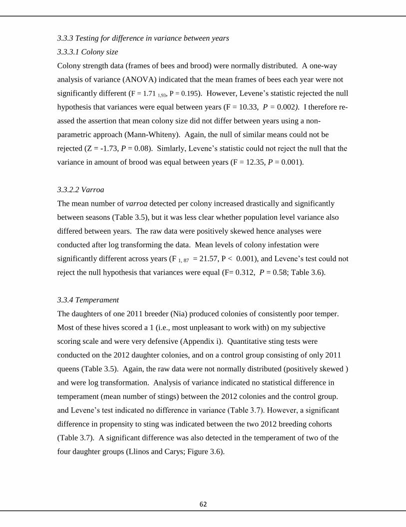
62
3.3.3 Testing for difference in variance between years
3.3.3.1 Colony size
Colony strength data (frames of bees and brood) were normally distributed. A one-way
analysis of variance (ANOVA) indicated that the mean frames of bees each year were not
significantly different (F = 1.71 1,93, P = 0.195). However, Levene’s statistic rejected the null
hypothesis that variances were equal between years (F = 10.33, P = 0.002). I therefore re-
assed the assertion that mean colony size did not differ between years using a non-
parametric approach (Mann-Whiteny). Again, the null of similar means could not be
rejected (Z = -1.73, P = 0.08). Simlarly, Levene’s statistic could not reject the null that the
variance in amount of brood was equal between years (F = 12.35, P = 0.001).
3.3.2.2 Varroa
The mean number of varroa detected per colony increased drastically and significantly
between seasons (Table 3.5), but it was less clear whether population level variance also
differed between years. The raw data were positively skewed hence analyses were
conducted after log transforming the data. Mean levels of colony infestation were
significantly different across years (F 1, 87 = 21.57, P < 0.001), and Levene’s test could not
reject the null hypothesis that variances were equal (F= 0.312, P = 0.58; Table 3.6).
3.3.4 Temperament
The daughters of one 2011 breeder (Nia) produced colonies of consistently poor temper.
Most of these hives scored a 1 (i.e., most unpleasant to work with) on my subjective
scoring scale and were very defensive (Appendix i). Quantitative sting tests were
conducted on the 2012 daughter colonies, and on a control group consisting of only 2011
queens (Table 3.5). Again, the raw data were not normally distributed (positively skewed )
and were log transformation. Analysis of variance indicated no statistical difference in
temperament (mean number of stings) between the 2012 colonies and the control group.
and Levene’s test indicated no difference in variance (Table 3.7). However, a significant
difference in propensity to sting was indicated between the two 2012 breeding cohorts
(Table 3.7). A significant difference was also detected in the temperament of two of the
four daughter groups (Llinos and Carys; Figure 3.6).
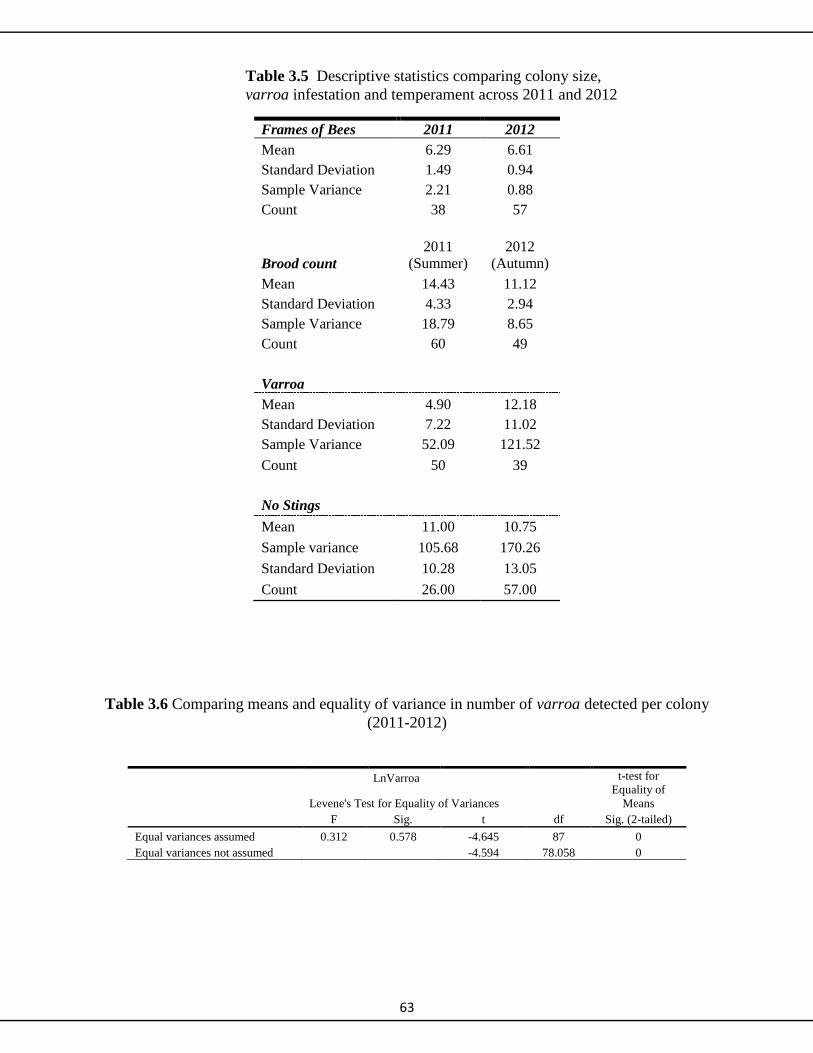
63
Table 3.5 Descriptive statistics comparing colony size,
varroa infestation and temperament across 2011 and 2012
Frames of Bees 2011 2012
Mean 6.29 6.61
Standard Deviation 1.49 0.94
Sample Variance 2.21 0.88
Count 38 57
Brood count
2011
(Summer)
2012
(Autumn)
Mean 14.43 11.12
Standard Deviation 4.33 2.94
Sample Variance 18.79 8.65
Count 60 49
Varroa Mean 4.90 12.18
Standard Deviation 7.22 11.02
Sample Variance 52.09 121.52
Count 50 39
No Stings
Mean 11.00 10.75
Sample variance 105.68 170.26
Standard Deviation 10.28 13.05
Count 26.00 57.00
Table 3.6 Comparing means and equality of variance in number of varroa detected per colony
(2011-2012)
LnVarroa t-test for
Equality of
Means
Levene's Test for Equality of Variances
F Sig. t df Sig. (2-tailed)
Equal variances assumed 0.312 0.578 -4.645 87 0
Equal variances not assumed
-4.594 78.058 0
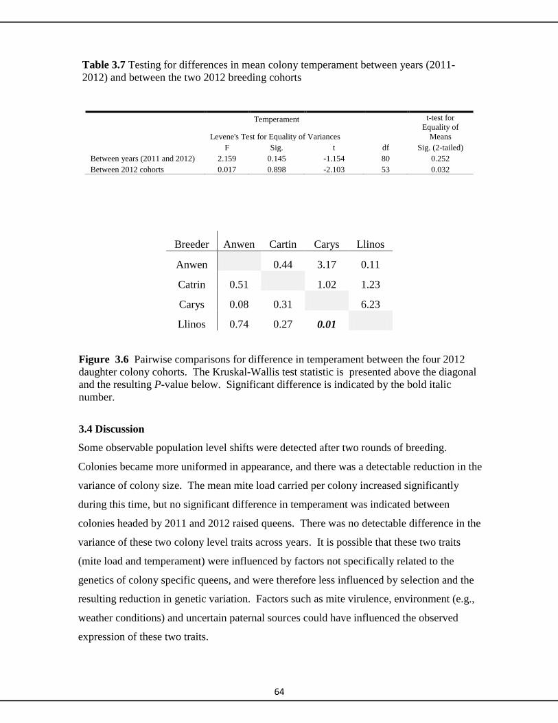
64
Table 3.7 Testing for differences in mean colony temperament between years (2011-
2012) and between the two 2012 breeding cohorts
Breeder Anwen Cartin Carys Llinos
Anwen 0.44 3.17 0.11
Catrin 0.51 1.02 1.23
Carys 0.08 0.31 6.23
Llinos 0.74 0.27 0.01
Figure 3.6 Pairwise comparisons for difference in temperament between the four 2012
daughter colony cohorts. The Kruskal-Wallis test statistic is presented above the diagonal
and the resulting P-value below. Significant difference is indicated by the bold italic
number.
3.4 Discussion
Some observable population level shifts were detected after two rounds of breeding.
Colonies became more uniformed in appearance, and there was a detectable reduction in the
variance of colony size. The mean mite load carried per colony increased significantly
during this time, but no significant difference in temperament was indicated between
colonies headed by 2011 and 2012 raised queens. There was no detectable difference in the
variance of these two colony level traits across years. It is possible that these two traits
(mite load and temperament) were influenced by factors not specifically related to the
genetics of colony specific queens, and were therefore less influenced by selection and the
resulting reduction in genetic variation. Factors such as mite virulence, environment (e.g.,
weather conditions) and uncertain paternal sources could have influenced the observed
expression of these two traits.
Temperament t-test for
Equality of
Means
Levene's Test for Equality of Variances
F Sig. t df Sig. (2-tailed)
Between years (2011 and 2012) 2.159 0.145 -1.154 80 0.252
Between 2012 cohorts 0.017 0.898 -2.103 53 0.032
65
Despite the frequently unfavorable weather conditions, each year approximately 75% of
the newly established nuclei acquired a laying queen. These results were at par with other
sites with more favorable weather conditions (e.g. Shropshire) where the queen cells had
been raised by a professional breeder. Selection of low quality larvae (e.g. poorly
nourished), or ones that are damaged during the grafting process, can affect the mating
success and ultimate quality of the queens, and evidence of possible supersedure was
observed in a small number of nuclei in 2012. It is thought that supersedure occasionally
occurs in colonies with immature queens since they can have a similar pheromone ‘signal’
to that of an aging or failing queen (limited brood pheromone in hive). No evidence of
inadequate mating as indicated by inferior brood patterns resulting from diploid drone
production was observed. Sixty one of 118 colonies were taken to the heather in 2011, and
relatively good weather produced nectar flows that allowed the experimental colonies to
expand.
There was no correlation between weight change during this flow period, and the estimated
strength of the colony. This observation can be explained if there was a large variance in
colony foraging efficiency; or in other words, that colonies of similar size tended to
accumulate stores at different rates. However, there was a correlation in 2011 between
frames of bees and colony weight at end of the heather season. Since increasing
production potential is a main project goal, colonies displaying above expected weight gain
(in relation to number of bees) were highlighted. Fifteen colonies met these criteria of
which thirteen were also highlighted by z-score analysis for further observation as potential
breeder stock. Weight gain during nectar flow (rather than weight at end of heather
season) was the productivity criteria used in the z-score analysis, so it was reassuring to
observe a general agreement between the two methods. The two colonies with above
average productivity, but rejected by z-score analysis either had bad temperament (Nia
1.18), or very high varroa count (Lucy29 1.2). (see Appendix i). The colony headed by
queen Marged 1.6 was also a notable standout. The colony recorded highest net weight-
gain during the nectar flow but failed to register above the mean expected weight at the end
of the season. Clearly, the production potential of this colony would be missed by relying
on colony weight only.
All matured nuclei were transferred to the heather for monitoring in 2012. The inferior
quality and short duration of the heather bloom, and the associated prolonged periods of
66
unsettled weather, provided little opportunity for strong nectar flows and foraging by bees
this year. Colonies did manage to expand and steadily gain weight during the first few
weeks on the moor, but colony weights started diminishing as the heather flows began to
shut down. The rate of weight decline was negatively correlated with the amount of bees
in the colony. This makes sense as more bees need more food, and honey stores will
deplete at a faster rate in larger colonies. There were no specific periods of strong nectar
flows on the heather in 2012; hence no attention was given to foraging efficiency when
comparing colonies. Overall weight gained during the whole period when some foraging
was possible was therefore used, in relation to colony size, when comparing colonies.
Generally though, conditions offered little opportunity to monitor productivity this season.
The propagation of varroa tolerance was always a desirable project goal. The need for
increasing resistance was highlighted by the heavy losses, attributed to overwhelming
varroa and associated virus pressures (DWV and parasitic mite syndrome) that were
incurred across the winter of 2010/11. Mite counts were taken each year while the hives
were on the heather, just as brood production was beginning to slow down and as mite
populations approached peak numbers. Although it is known that mite count is only
marginally heritable (Harbo and Harris, 1999) counts were taken in an effort to selectively
direct the population towards tolerance.
Counts were also conducted to monitor population level infestation rates. Relatively low
numbers were detected in the experimental colonies 2011, possibly as a result of the
selective sweep the population incurred the previous winter. Numbers increased the
following year, (2012) and colonies were treated with an organic acid (3.5% oxalic acid
dribble) after brood production had stopped. The situation provided an apparent dilemma;
how can one now select for tolerance to local mite parasitism after drastically interfering
with host/pest interactions? Commercial operations have limited time and resources to
expend on demanding monitoring schedules. Recommendations based on a German
approach (Büchler et al. 2010) for evaluating varroa mite tolerance in honeybees were
recently proposed by the BEE DOC (Bees in Europe and the Decline Of honeybee
Colonies) project. The method suggests taking two varroa counts (one in the spring and
the other later in the summer) to assess mite population growth rates. The process seems
well suited for use by well-resourced institutional breeding organizations, and less so by
67
small scale breeding programs trying to improve overall bee performance by merely
selecting from the constantly strongest performing colonies
Bee temperament was unusually bad during the spring of 2012, and although weather
conditions were poor and known to influence temper (Villa, 1988), there was concern that
the aberrant behaviour was due to breeding. A distinct difference in propensity to sting
was demonstrated among the 2012 experimental colonies. However, overall, there was no
significant difference between the 2012 experimental population and a control group
comprising of 2011 and earlier colonies only. Neither the mean number of stings per
colony, nor the variance of the data was statistically different between groups. These
assays were conducted after both groups had been migrated to the heather and under very
similar weather conditions days apart. These results seem to suggest that environmental
conditions may have been the major contributing factor affecting colony temperaments
earlier in the year.
However, stinging response is known to have a genetic component (heritability). For
example, there are three known stinging behaviour QTL’s: sting-1, sting-2 and sting-3
(Arechavaleta-Velasco, et al., 2003), with sting-1 being associated with actual stinging
response and guarding. Beekeepers commonly try to remedy unmanageable hives by
replacing the queen. The new queen mediates the transfer of both maternal (from her) and
paternal (from the drones she mated with) sting genes into the next generation of diploid
workers. It is possible that colony defensiveness can be directly influenced by the colony
queen genotype, or indirectly by the haplotypes of the drones she mated with.
Two groups of daughter queens were grafted in the spring of 2012. Each group comprised
of daughter colonies raised from the same four breeders, but they were located in different
mating apiaries. There was a significant difference in the defensiveness of the two groups
when possible maternal effects were ignored. Overall, daughter colonies from the first
grafting batch were statistically less defensive than the colonies from the second.
Comparing within breeder groups showed that this overall difference was driven mainly by
the highly significant difference observed between the two grafting sister-groups of one
specific breeder (Llinos). However, a general trend was obvious as there was an almost
significant difference between grafting cohort for two of the other three breeders.
Numerous environmental variables could have potentially differentially affected the

68
development and conditioning of the queen larva in these two grafted groups, but it is
unknown if such non-inherited influences can affect the temperament of a queens progeny.
Mating success is largely environment dependent and there may have differed between
groups, but again there is no evidence that a correlation exists between mating success and
progeny temperament. Mating success is known to influence queen development and
conditioning (Tarpy et al., 2012; Richard et al., 2007) which in turn affects her pheromone
induced influence over colony behaviour.
It is also possible (and probably most likely) that difference between grafting cohorts
reflects a paternal genetic influence since drone contribution and conditions may have
differed. This explanation is very plausible since these two groups mated at different
locations occupied by different drone contributing colonies. Different colonies contributed
drones to these two groups. Guzman-Novoa et al. (2004) describe the influence of paternal
gene transfer on colony level defensive response. They conducted reciprocal cross
experiments between honeybee colonies of European and African origin, and observed that
hybrid colonies of African paternity were significantly more defensive. They hypothesized
that epigenetic influences might be down-regulating (silencing through methylation) major
stinging alleles if inherited from the mother in order to reduce the cost associated with
having an overly defensive and ‘unbalanced’ colony. Many drones usually contribute to
colony phenotype; hence major defensive alleles will by chance be inherited by a fraction
of workers only. Colonies might therefore have a more ‘balanced’ defensive response if
the trait is inherited through the male line. The authors hypothesized a gender specific
silencing mechanism and suggest that major defense alleles may not be silenced when
inherited from the father.
Assuming the above hypothesis is true; bee-breeders may not be readily able to identify
colonies producing drones carrying major defense allele, as these alleles will be silenced in
workers when inherited from the queen. But a high percentage of the drones produced by
the queen will carry these alleles, and if they successfully mate, their effect will be
expressed in the daughters; i.e. the workers in colonies headed the queens they mate with.
Colonies headed by queens that mated with multiple drones carrying major defense alleles
may become defensive and difficult to manage when.

69
Although 11 and 4 breeders were selected in 2011 and 2012 respectively, the effective
number used each year approximated 8.3 and 3.5 due to unequal breeder representation in
the daughter generation. Greater selection pressure was therefore applied during the
second round of breeding (2012). There was consequently greater uniformity among the
2012 colonies in both size and organization of the brood nest. This noticeable trend was
statistically supported since there was significantly less variance in the numbers of frames
of bees occupied by bees at the end of the 2012 season, although there was no difference in
means across years. Reduced variance was also noted for brood amount in each nest.
Means were also different in this case since comparisons were made using data collected at
different times of the year (summer and autumn), and therefore during different colony
development periods. However, this trend towards uniformity was notable and suggests
that the population as a whole is responding to selection pressure.
One of the goals of the WWBBP is to develop a practical protocol that could help small
breeding programs improve the quality of their bees. Broadly, the ‘improved’ population
will trend towards greater productivity, greater disease resistance and gentleness with time.
The program has gone through two rounds of selection to date, and there is slim evidence
of “improvement”. Nevertheless, a trend towards uniformity is clearly indicated by
observation and by a statistically significant reduced variance in colony characteristics.
The program selected 11 breeders in 2011 and dropped this number to 4 in 2012. Four
breeders per generation is the current favored model, a number driven mostly by practical
and logistical co considerations, since the program can only accommodate a limited
number of new colonies a year (n ~ 80 to 100).
Queen ‘rearing’ might aid beekeepers to treat the symptoms of poor bee-health (i.e.
replacing losses), but it does not necessarily address the root cause of unacceptably high
mortality. At worst, an unconsidered approach to rearing could inadvertently exacerbate
future overwintering losses and general bee-health (e.g. genetically constrained selection
regime). A basic understanding of bee mating biology and the genetic dynamics of bee
populations might help avoid such pitfalls. Research has consistently demonstrated a
correlation between degree of genetic diversity and general health and fitness at both
colony and population level. Genetically depleted colonies or populations have been
shown to express reduced vigor and increased susceptibility to disease. Breeders must
guard against genetic depletion by rearing queens from unrelated breeders.

70
Monitoring phenotypic change revealed three key points. First, colony size responded to
selection, becoming more uniformed as the population became more genetically
constrained. This observation was interpreted as a consequence of effective breeder
number dropping to only four in 2012. Secondly, the mean number of varroa mites
detected per colony increased drastically between years. The program suffered serious
varroa attributed losses in 2011, hence these results demonstrate the value of monitoring as
a tool to manage colony treatment. Lastly, a difference in temperament between the two
2012 breeding cohorts (each comprising of daughters raised from the same four breeders,
but mated at different locations) suggest that paternal influences might be affecting overall
temperament.
71
Chapter 4
Selection on Genetics

72
4.1 Introduction
Line breeding is a common breeding design used by small scale breeders selecting and
breeding from within a small closed population (the line). Small operations, such as the
West Wales Bee Breeding Program (WWBBP), can generally only resource a single line,
within which a limited number of individual queen lines will be maintained. Within-
family selection has been recommended when working with relatively small populations
such as this (Moritz, 1986). It is considered as the best approach for small scale operators
wanting to improve stock quality while concurrently trying to maintain genetic diversity
across generations. The basic approach is to each year select and breed from the best
performing colony in each breeder family. In conjunction with queen selection, one can
also simultaneously manipulate male mediated contributions by using the drones produced
by sister queen cohorts that had been raised from strong and vigorous colonies the previous
summer. These drones would mediate the transfer of promising grandmother colony
characteristics through the male line. This approach has been loosely applied by the
WWBBP to date.
4.1.1 Avoiding inbreeding
Charles Darwin (1876) was the first to formally describe the detrimental effects of
inbreeding. He demonstrated this by comparing the fitness effects of cross and self-
fertilization in numerous plant species. Since then, innumerable studies on both wild and
captive populations have demonstrated similar effects in sexually producing organisms.
Crnokrak and Roff (1999) subsequently published a significant work suggesting that wild
inbred individuals will on average suffer seven times more from the effects of inbreeding
depression than similarly inbred captive individuals. Inbreeding depression appeared to be
expressed to a greater extent under stressful circumstances. The increased rates of colony
losses observed in the Northern hemisphere over recent years indicate that honeybees are
experiencing a period of increased stress. It is possible that the multifaceted nature of
these challenges could render bees more susceptible to the expression of detrimental
inbreeding effects.
Inbreeding is an inevitable consequence of line-breeding (Harbo and Rinderer, 1980) since
selection constricts the transfer of genetic material across generations. Inbreeding will
eventually be detrimental to breeding efforts since enhancing the expression of desired

73
characteristics becomes more difficult with each passing generation as selecting for
desirable traits will be far less effective in inbred populations. Colonies with inbred bees
might also express reduced vigor and may have spotty brood pattern (glossary) due to
homozygosity at the sex determination locus. It is commonly argued that the social
hymenoptera are particularly susceptible to inbreeding depression due to genetic load on
the sex determination locus (csd) and to their usually low effective population sizes (Zayed
and Packer, 2005) In reality, little is known about the effects of inbreeding in haplodiploid
insects (Liautard and Sundström, 2005) and there seems to be limited evidence that it is a
problem in large managed commercial beekeeping operations that use open mating
(Oldroyd, 2012).
Two hypotheses (dominance and over-dominance) are frequently evoked to explain the
expression of inbreeding depression (Zayed, 2009). Firstly, diploid individuals randomly
mating in a large population carrying lethal and non-lethal alleles at low frequency will be
protected from the deleterious effects of rare maladapted alleles by the masking effect of
dominant non-deleterious homologs (dominance). The expression of inbreeding
depression becomes more likely in small closed populations due to the increased likelihood
that maladaptive alleles become paired due to mating between relatives. In addition,
random genetic drift in small populations reduces genetic diversity (since alleles are more
likely to be lost in small populations) leading to increased homozygosity and increased
likelihood of inbreeding depression (Lande, 1988). The accumulated effect of numerous
homozygous loci carrying maladapted genes results in general loss of vigor. This in effect
is inbreeding depression. The second hypothesis relating to inbreeding is over-dominance,
which suggests that inbreeding is caused by the tendency of homozygotes to have lower
overall fitness than heterozygotes.
4.1.2. Genetic variation in honeybee populations
Honeybees have been managed by humans for thousands of years and extensively so in
Europe and North America since the middle of the nineteenth century. Domestication in
general usually results in loss of genetic diversity (Wright et al., 2005; Zeder et al., 2006)
and low levels of genetic diversity have been observed in several European and North
American populations (Delaney, et al., 2009; Jaffé et al., 2010; Meixner et al., 2010). In
light of the very poor health of many contemporary managed populations (Cobey et al.,
2012; vanEngelsdorp and Meixner, 2009) these observations have raised concern that
74
historical bee management and breeding practices may have resulted in a depleted
contemporary genetic pool. Many studies have correlated increased diversity with superior
colony robustness and vitality hence the maintenance of variation is important.
However, honeybees are not strictly ‘domesticated’ and recent work by Harpur, et al.
(2012) indicates that managed admixed populations of honeybees in Europe have more
genetic diversity than either of their two progenitor populations, i.e., the Western (M) and
the Eastern (C) lineages (Franck et al., 1998; Garnery et al., 1992; Whitfield et al., 2006).
Genetic and morphological methods indicate that honeybees spread out of Africa during
two separate expansion events and that they were historically geographically isolated into
North West and South East Europe. The translocation of bees between these regions was
begun by beekeepers and breeders during the middle of the nineteenth century and
continues to this day (Meixner et al., 2010). It appears that the constant input of imported
stock and the somewhat novel mating biology of honeybees may have allowed diversity to
be maintained despite the selection pressures that are applied due to management practices
(Harpur et al., 2012; Oldroyd, 2012). There is also evidence from large breeding
operations using open mating that neutral genetic diversity is maintained (Oldroyd, 2012).
4.1.3 Effective population size
Population size (N) is a central tenet of evolutionary theory since it has a profound bearing
on the response of populations to drift and selection, and on their susceptibility to
inbreeding (Waples, 1989). Simple counts or mark recapture methods can provide
accurate populations estimates, but the census size can also differ greatly from its effective
genetic size (Ne). Ne can be defined as the number of individuals contributing genes to the
next generation, but is more equivalent to the number of colonies within effective mating
range for honeybees. Consequently, numerous estimators utilizing molecular data from
population samples have been developed. These approaches have been used by wildlife
managers concerned about the destiny of small populations since they can provide insight
into potentially problematic demographic and genetic trends. I employed these methods to
investigate changes in population size in a managed honeybee population over a brief
contemporary time scale due to selection.
4.1.4 Microsatellite loci and the Complementary Sex Determination (csd) locus
75
I used a suite of selectively neutral markers and a single marker from a region under strong
selection to assess how much genetic variation was in the baseline population.
Microsatellite loci are generally assumed to reside in selectively neutral regions of no
known function. They are characterized as regions with high mutation rates comprising of
two, three, or four base pair repeat sequence motifs bounded by more conserved regions of
locus specific sequences. These bordering regions provide primer access for fragment
amplification using PCR. Conversely, csd is a gene with a described sex-determination
function that experiences balancing selection in response to diploid drone production.
Bees that are homozygous at the csd locus develop into sterile diploid drones that can
contribute nothing to the next generation. Low frequency csd alleles are therefore favored
as they are less likely to match in a homozygous diploid state with zero fitness.
In this chapter I investigate the rate of genetic change occurring in a breeding population
under selection across two breeding cycles. The population comprised mainly of bees that
had been sourced, over a number of years, from a knowledgeable local bee breeder who
had likely taken steps to avoid inbreeding. In light of this knowledge, and of the recent
work by Harpur et al. (2012) highlighting the increased genetic diversity found due to
translocation in managed bee populations, I considered it likely that high levels of
polymorphism would be found at both neutral microsatellite loci, and at the csd locus in
this population. I also hypothesized that there would be a detectable reduction as a result
of selection in both genetic diversity and effective population size (Ne) across the
monitoring period.
4.2 Methods
4.2.1. Population genetic data sampling
Sampling was designed to investigate the rate of genetic change occurring in a breeding
population under selection across two breeding cycles. Samples were taken from the
source population (G0) which was comprised of colonies that were established in 2010 or
earlier. Foraging workers were sampled from the entrance of sixty randomly selected
colonies. The 2011 (G1) and 2012 (G2) ‘cohort’ data were generated using worker
samples taken from colonies headed by queens raised during the respective year. The
WWBBP selected eight effective breeders from the baseline population to supply queens
for the 2011 cohort, and four breeders were selected from this cohort to supply queens for

76
2012. The daughter colonies of the 2011 (G1) and 2012 (G2) breeders were sampled in a
similar fashion to the baseline, with sixty foragers (colonies) sample each year. All
samples were stored in 98% ethanol at room temp for preservation and DNA extraction.
4.2.2 DNA extraction
DNA was extracted from equal volumes of leg or thorax tissue using a modified version of
the 96 well plate protocol described by Lagisz et al.(2010). The extraction protocol was
performed in 1.5ml tubes and the reagent volumes adjusted accordingly. The cell lysis was
conducted under moderate agitation at 37°C using a solution comprised of 50mM Tris (pH
8.0), 0.4M NaCl, 0.5% SDS and 20mM EDTA. Lysing was allowed to proceed for two or
three days for higher yields. Salt precipitation with 4M Ammonium Acetate was used to
precipitate unwanted cell proteins. The salt solution was added to the lysis mixture and
centrifuged. The DNA-containing supernatant was poured into anther tube, and
precipitated out of solution with ethanol. This tube was centrifuged for 30 minutes to
pellet the DNA and the ethanol carefully poured off. After a final wash step using 70%
ethanol and a 12-15 min spin, the DNA pellet was left overnight on the bench to dry and
rehydrates in 50µl of 1X TE. The extracted DNA was quantified using a NanoDrop
nd1000 spectrophotometer and each sample was diluted to 50ng/µl for genotyping.
4.2.3 PCR Multiplex Systems
I designed two multiplex reactions comprising of seven and three microsatellite primer
pairs each (Table 4.1). Each multiplex was amplified in a single 10µl multiplexed reaction
consisting of 50 ng of DNA, 0.75 X Qiagen multiplex PCR solution, 2.5 and 0.25 pM of
reverse and forward primer mixes respectively, and 2.5pM of ABI Fam-, Pet- and Ned-
and 5.0pM of Vic-labeled primer. Polymerase chain reactions were performed on a DNA
engine Tetrad 2 thermocycler (BIO RAD) using the following cycling parameters: 95°C
for 15 min, followed by 13 cycles of 94°C for 45 sec, 55°C for 45 sec and 72°C for 45 sec,
and then 25 cycles of 94°C for 45 sec, 52°C for 45 sec, and 72°C for 45 sec. The profile
was terminated with a 30 min extension at 60°C. Reaction products were visualized on an
ABI 3130xl Genetic Analyzer and the data were analyzed using Genemapper (ABI).
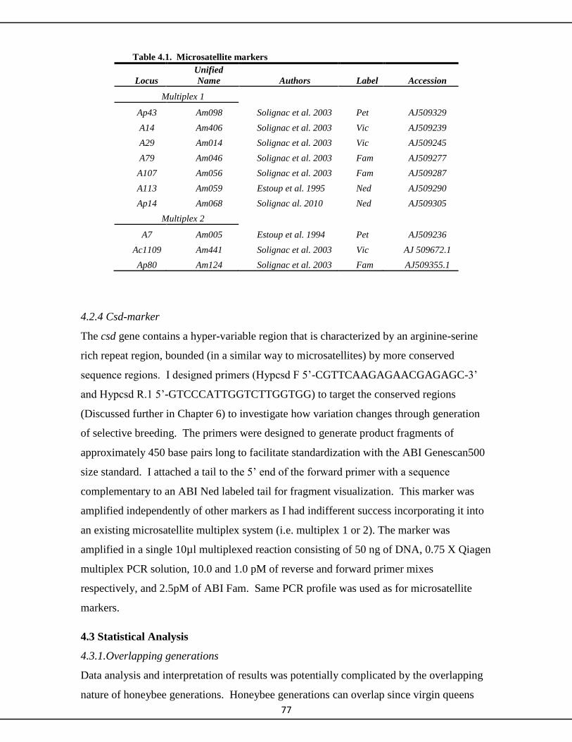
77
Table 4.1. Microsatellite markers
Locus
Unified
Name Authors Label Accession
Multiplex 1
Ap43 Am098 Solignac et al. 2003 Pet AJ509329
A14 Am406 Solignac et al. 2003 Vic AJ509239
A29 Am014 Solignac et al. 2003 Vic AJ509245
A79 Am046 Solignac et al. 2003 Fam AJ509277
A107 Am056 Solignac et al. 2003 Fam AJ509287
A113 Am059 Estoup et al. 1995 Ned AJ509290
Ap14 Am068 Solignac al. 2010 Ned AJ509305
Multiplex 2
A7 Am005 Estoup et al. 1994 Pet AJ509236
Ac1109 Am441 Solignac et al. 2003 Vic AJ 509672.1
Ap80 Am124 Solignac et al. 2003 Fam AJ509355.1
4.2.4 Csd-marker
The csd gene contains a hyper-variable region that is characterized by an arginine-serine
rich repeat region, bounded (in a similar way to microsatellites) by more conserved
sequence regions. I designed primers (Hypcsd F 5’-CGTTCAAGAGAACGAGAGC-3’
and Hypcsd R.1 5’-GTCCCATTGGTCTTGGTGG) to target the conserved regions
(Discussed further in Chapter 6) to investigate how variation changes through generation
of selective breeding. The primers were designed to generate product fragments of
approximately 450 base pairs long to facilitate standardization with the ABI Genescan500
size standard. I attached a tail to the 5’ end of the forward primer with a sequence
complementary to an ABI Ned labeled tail for fragment visualization. This marker was
amplified independently of other markers as I had indifferent success incorporating it into
an existing microsatellite multiplex system (i.e. multiplex 1 or 2). The marker was
amplified in a single 10µl multiplexed reaction consisting of 50 ng of DNA, 0.75 X Qiagen
multiplex PCR solution, 10.0 and 1.0 pM of reverse and forward primer mixes
respectively, and 2.5pM of ABI Fam. Same PCR profile was used as for microsatellite
markers.
4.3 Statistical Analysis
4.3.1.Overlapping generations
Data analysis and interpretation of results was potentially complicated by the overlapping
nature of honeybee generations. Honeybee generations can overlap since virgin queens

78
can mate with drones produced by much older queens and drone-producing queens can
persist for multiple years under natural circumstances. Samples taken from the source
population were assumed to be a random sample of a single generation consisting of 2010
and older queens. This sample set was inherently different to the samples subsequent taken
from annually produced cohorts groups (G1 and G2). I therefore compared the genetic
signature of the source population to each of the cohort years separately, and to the two
cohort years combined as a single ‘generation’.
4.3.2 Genetic diversity
Genetic diversity has been measured in a number of different ways. Heterozygosity is a
very commonly used index. It is the expected probability that an individual carries
different alleles (heterozygote) at a single locus, or at an assay of different loci,
∑∑
where, pi is the frequency of the ith
of k alleles, and m is the number of loci. The observed
heterozygosity (Ho) in a population sample is frequently compared to that which would be
expected (He) under conditions of random mating. Significant deviations will indicate that
the population is experiencing an external driver or evolutionary force such as selection or
inbreeding. Average heterozygosity is a measure of genetic diversity at the population
scale and indicates the average proportion of individuals that are heterozygous for any
given trait (locus).
The mean number of alleles per locus (Allelic Richness) is another commonly reported
diversity index. It is very sensitive to sample size, and has the disadvantage that
information is lost due to rarefaction. Rarefaction is used to determine this index. It
allows number of allele estimates from samples of different sizes to be compared, but it
does this by scaling from all samples data down to that of the lowest sample size.
Nevertheless, the method is useful since it is more sensitive than changes in observed

79
heterozygosity to recent bottleneck events since it is more sensitive to the loss of low
frequency alleles.
Exact tests for Hardy Weinberg Equilibrium (HWE) for each locus and ‘population’, and
genotypic linkage disequilibrium among loci pairs within each population, were computed
in GENEPOP (on the web version 4.0.14), and Arlequin (version 3.5.1). Arlequin was also
used to investigate genetic structure over all loci between sampling years. FSTAT was
used to determine expected and observed heterozygozity and to determine the number of
alleles per locus (Allelic Richness) per generation.
Friedman’s test (SPSS v.19) was used to test for significant differences in allelic richness
and expected heterozygozity across sampling years. Each ‘population’ is ranked according
to its diversity at a particular locus the average rank of each population across all loci is
then calculated and the null hypothesis that the ranks do not differ from the expected value
is tested using chi-square.
4.3.3 Detecting bottlenecks
The program Bottleneck version 1.2.02 (Cornuet and Luikart, 1996) was also used to try
and detect recent reductions in effective population size. Populations that undergo a
bottleneck event suffer reductions in allele numbers and a corresponding, but delayed
reduction, in observed heterozygozity. That is, the heterozygosity observed immediately
post bottleneck will be greater than that expected with the observed allele frequencies (for
loci in mutation-drift equilibrium).
Bottleneck runs a “sign test", a "standardized differences test" (Cornuet and Luikart, 1996),
and a "Wilcoxon sign-rank test" to test for excess heterozygosity. However, the
standardized difference test was not appropriate since a minimum of 20 loci is
recommended and it assumes normal distribution of heterozygosity across loci. The
Wilcoxon sign test does not assume a normal distribution and tests the hypothesis that the
values of HE (expected heterozygosity) from the baseline and post selection cohorts (both
separately and combined) were not different (Spencer et al., 2000). The program returns
heterozygosity values expected under mutation-drift equilibrium for the Infinite Allele
Model (I.A.M), the Stepwise Mutation Model (S.M.M), and the Two Phase Model
(T.M.P), and computes if these values are greater or less than would be expected for each
model. It provides a P -value for each observed heterozygosity. I report results for all
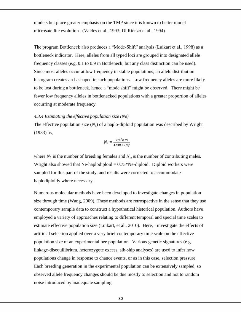
80
models but place greater emphasis on the TMP since it is known to better model
microsatellite evolution (Valdes et al., 1993; Di Rienzo et al., 1994).
The program Bottleneck also produces a “Mode-Shift” analysis (Luikart et al., 1998) as a
bottleneck indicator. Here, alleles from all typed loci are grouped into designated allele
frequency classes (e.g. 0.1 to 0.9 in Bottleneck, but any class distinction can be used).
Since most alleles occur at low frequency in stable populations, an allele distribution
histogram creates an L-shaped in such populations. Low frequency alleles are more likely
to be lost during a bottleneck, hence a “mode shift” might be observed. There might be
fewer low frequency alleles in bottlenecked populations with a greater proportion of alleles
occurring at moderate frequency.
4.3.4 Estimating the effective population size (Ne)
The effective population size (Ne) of a haplo-diploid population was described by Wright
(1933) as,
Ne =
where Nf is the number of breeding females and Nm is the number of contributing males.
Wright also showed that Ne-haplodiploid = 0.75*Ne-diploid. Diploid workers were
sampled for this part of the study, and results were corrected to accommodate
haplodiploidy where necessary.
Numerous molecular methods have been developed to investigate changes in population
size through time (Wang, 2009). These methods are retrospective in the sense that they use
contemporary sample data to construct a hypothetical historical population. Authors have
employed a variety of approaches relating to different temporal and special time scales to
estimate effective population size (Luikart, et al., 2010). Here, I investigate the effects of
artificial selection applied over a very brief contemporary time scale on the effective
population size of an experimental bee population. Various genetic signatures (e.g.
linkage-disequilibrium, heterozygote excess, sib-ship analyses) are used to infer how
populations change in response to chance events, or as in this case, selection pressure.
Each breeding generation in the experimental population can be extensively sampled, so
observed allele frequency changes should be due mostly to selection and not to random
noise introduced by inadequate sampling.
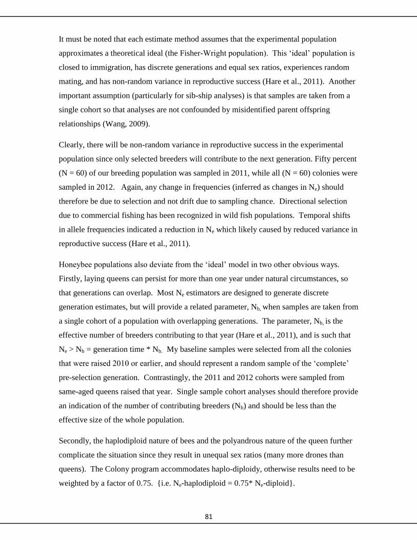
81
It must be noted that each estimate method assumes that the experimental population
approximates a theoretical ideal (the Fisher-Wright population). This ‘ideal’ population is
closed to immigration, has discrete generations and equal sex ratios, experiences random
mating, and has non-random variance in reproductive success (Hare et al., 2011). Another
important assumption (particularly for sib-ship analyses) is that samples are taken from a
single cohort so that analyses are not confounded by misidentified parent offspring
relationships (Wang, 2009).
Clearly, there will be non-random variance in reproductive success in the experimental
population since only selected breeders will contribute to the next generation. Fifty percent
(N = 60) of our breeding population was sampled in 2011, while all (N = 60) colonies were
sampled in 2012. Again, any change in frequencies (inferred as changes in Ne) should
therefore be due to selection and not drift due to sampling chance. Directional selection
due to commercial fishing has been recognized in wild fish populations. Temporal shifts
in allele frequencies indicated a reduction in Ne which likely caused by reduced variance in
reproductive success (Hare et al., 2011).
Honeybee populations also deviate from the ‘ideal’ model in two other obvious ways.
Firstly, laying queens can persist for more than one year under natural circumstances, so
that generations can overlap. Most Ne estimators are designed to generate discrete
generation estimates, but will provide a related parameter, Nb, when samples are taken from
a single cohort of a population with overlapping generations. The parameter, Nb, is the
effective number of breeders contributing to that year (Hare et al., 2011), and is such that
Ne > Nb = generation time * Nb. My baseline samples were selected from all the colonies
that were raised 2010 or earlier, and should represent a random sample of the ‘complete’
pre-selection generation. Contrastingly, the 2011 and 2012 cohorts were sampled from
same-aged queens raised that year. Single sample cohort analyses should therefore provide
an indication of the number of contributing breeders (Nb) and should be less than the
effective size of the whole population.
Secondly, the haplodiploid nature of bees and the polyandrous nature of the queen further
complicate the situation since they result in unequal sex ratios (many more drones than
queens). The Colony program accommodates haplo-diploidy, otherwise results need to be
weighted by a factor of 0.75. {i.e. Ne-haplodiploid = 0.75* Ne-diploid}.

82
Finally, the relatively short nature of this study limits the precision of the two samples for
estimating Ne methods described below. For precision, it is recommended that a sample-
span of two or more generations be used with these methods. I include a discussion and
report results on their use below of completeness, but will concentrate single sample results
which generally report Ne on the previous generation.
4.3.4a Estimating Ne using single sample approaches
These methods are appealing since only one sample from the monitored population is
required. One does not have to wait for generations and a second round of sampling. They
estimate Ne by using genetic signatures observed in the one sample data using patterns
related to various genetic parameters including linkage among alleles from different loci,
heterozygosity and patterns of relatedness among sampled individuals. Recent
developments have benefited from recent advances in computing capacity and have shown
promising results with these approaches (Hare et al., 2011). For example, Waples and Cho
(2008) recently published LDNE which has a bias correction for estimates of (Ne) based on
linkage disequilibrium data, and Wang (2009) developed the sib-ship assignment (SA)
method for estimating Ne from single generation samples. The method is implemented in
the program Colony (Jones and Wang, 2010) and relies on the fact that individuals from
the same cohort are more likely to be related (as-sibs) in small populations. Individuals are
more likely to share a common parent or parents when the parental cohort is small. All Ne
estimates make assumptions about the sampling protocols and populations. The SA
method is most sensitive to deviations from single cohort sampling since individuals from
different cohorts could be parent-offspring and mistakenly assigned as sibs. Such false
assignments would mistakenly lower Ne.
4.3.4b Estimating Ne using temporally based methods
Temporally based methods utilize changes in allele frequencies across generations and
hence require at least two different temporal samples from the population of interest. The
methods work best when the degree of change due to drift or (as in our case) selection is
large since the disruptive effects of changes due to random drift are drowned out of the
“signal”. These methods should therefore be applicable to a selective breeding situation
since we should be imposing enough selection to impose an adaptive response from out
population. We can also accommodate large and very accessible sample numbers (large
numbers of bees in a colony) in relation to relatively small population sizes. Returned

83
values should therefore indicate changes due to selection as opposed to random drift due to
sampling effect. Additionally, sampling more loci enhances precision (Waples, 1989).
4.3.5 Moment-based temporal methods
Moment-based methods utilize the relationship between Wright’s F statistic (1951) and
genetic drift. One formulation of F utilizes the expected variance in allele frequency (pt)
between time 0 and t, when adjusted for its starting frequency [p0 (1- p0)], and is given as,
( )
( ) = ( )
( )
when (
) is less than 0.15 (Nei and Tajima, 1981). The expectation of F can therefore
be estimated from the observed variance in allele frequencies across samples since this
result can be converted to give an estimate of Ne.
It is thought that these methods tend to upwardly bias the estimator when low frequency
alleles are encountered. Highly variable microsatellite markers are susceptible to this
source of bias since they might carry numerous alleles at low frequency. Bias is also
introduced if drift (or selection in our case) is strong enough to result in loss of alleles
between samples (Waples, 1989). Precision improves and bias due to overlapping
generations decreases with increasing number of breeding cycles between sampling
(Waples and Yokota, 2007).
4.3.5a Coalescent based temporal method (TM3)
I also used the program TM3 (Berthier et al., 2002). This approach applies the coalescent
model in a temporal method framework. The model is based on the higher expected rates
of coalescence when historical populations are small. The convers will also apply, and
lower rates of coalescence should occur between the recent and historic samples when
historic populations are large. Coalescence based estimators can more readily
accommodates continuously reproducing (overlapping generations) populations rather than
models based on discrete-generation Wright-Fisher populations (Anderson, 2005). I ran
this method multiple times to ensure consistent results.
4.4 Results
4.4.1 Microsatellites (neutral markers)
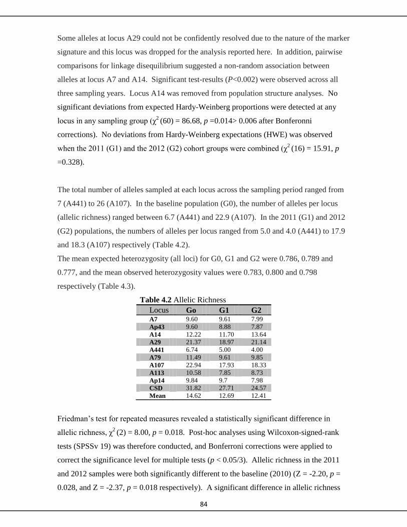
84
Some alleles at locus A29 could not be confidently resolved due to the nature of the marker
signature and this locus was dropped for the analysis reported here. In addition, pairwise
comparisons for linkage disequilibrium suggested a non-random association between
alleles at locus A7 and A14. Significant test-results (P<0.002) were observed across all
three sampling years. Locus A14 was removed from population structure analyses. No
significant deviations from expected Hardy-Weinberg proportions were detected at any
locus in any sampling group (χ2
(60) = 86.68, p =0.014> 0.006 after Bonferonni
corrections). No deviations from Hardy-Weinberg expectations (HWE) was observed
when the 2011 (G1) and the 2012 (G2) cohort groups were combined (χ2
(16) = 15.91, p
=0.328).
The total number of alleles sampled at each locus across the sampling period ranged from
7 (A441) to 26 (A107). In the baseline population (G0), the number of alleles per locus
(allelic richness) ranged between 6.7 (A441) and 22.9 (A107). In the 2011 (G1) and 2012
(G2) populations, the numbers of alleles per locus ranged from 5.0 and 4.0 (A441) to 17.9
and 18.3 (A107) respectively (Table 4.2).
The mean expected heterozygosity (all loci) for G0, G1 and G2 were 0.786, 0.789 and
0.777, and the mean observed heterozygosity values were 0.783, 0.800 and 0.798
respectively (Table 4.3).
Table 4.2 Allelic Richness
Locus Go G1 G2 A7 9.60 9.61 7.99
Ap43 9.60 8.88 7.87
A14 12.22 11.70 13.64
A29 21.37 18.97 21.14
A441 6.74 5.00 4.00
A79 11.49 9.61 9.85
A107 22.94 17.93 18.33
A113 10.58 7.85 8.73
Ap14 9.84 9.7 7.98
CSD 31.82 27.71 24.57
Mean 14.62 12.69 12.41
Friedman’s test for repeated measures revealed a statistically significant difference in
allelic richness, χ2
(2) = 8.00, p = 0.018. Post-hoc analyses using Wilcoxon-signed-rank
tests (SPSSv 19) was therefore conducted, and Bonferroni corrections were applied to
correct the significance level for multiple tests (p < 0.05/3). Allelic richness in the 2011
and 2012 samples were both significantly different to the baseline (2010) (Z = -2.20, p =
0.028, and Z = -2.37, p = 0.018 respectively). A significant difference in allelic richness

85
was also detected between the source population and the two cohort sample groups
combined (Z = -2.028, P = 0.022 1-tailed). There was no significant difference in allelic
richness between the 2011 and 2012 samples (Z= -1.352, p = 0.176) and no statistically
significant difference in expected heterozygosity (χ2
(2) = 1.143, p = 0.565) between any of
the sampling periods.
4.4.2 Complementary sex determination (csd)
A total of 44 different fragment lengths were detected in the hyper-variable region of the
csd gene. These fragments ranged in size from 407 to 493 base pairs long, with 33, 28 and
25 ‘alleles’ detected in G0, G1 and G2 respectively. There was a consistent decline in
number of alleles detected each year at this locus, and a corresponding drop in allelic
richness at this locus across the sampling period (Table 4.2). Since this locus experiences
strong selection, and will behave differently to microsatellites in evolutionary terms, it was
removed from further analysis.
Table 4.3. Expected and observed
heterozygosities at all markers Locus G0 G1 G2
Expected
A7 0.73 0.79 0.79
Ap43 0.79 0.84 0.82
A14 0.80 0.82 0.86
A29 0.90 0.91 0.90
A441 0.65 0.54 0.56
A79 0.80 0.79 0.79
A107 0.93 0.92 0.91
A113 0.77 0.81 0.75
Ap14 0.79 0.80 0.7
CSD 0.93 0.94 0.94
Mean 0.81 0.82 0.81
Observed
A7 0.72 0.72 0.84
Ap43 0.85 0.88 0.78
A14 0.78 0.84 0.85
A29 0.86 0.92 0.87
A441 0.60 0.62 0.62
A79 0.81 0.81 0.83
A107 0.87 0.92 0.89
A113 0.76 0.72 0.74
Ap14 0.84 0.89 0.85
CSD 0.86 0.92 0.90
Mean 0.79 0.83 0.82

86
4.4.3. Bottleneck
All sample groups had significant heterozygote excess under the IAM. Significant P-
values were also returned by the Wilcoxon-signed-rank test for the 2011 and 2012 samples
under the T.M.P model and by the sign rank tests in the 2012 samples under S.M.M (Table
4.4a). Similarly, Bottleneck detected significant heterozygote excess when both cohort
years were combined as one. Again, the Wilcoxon signed rank test indicated significant
heterozygote excess under the T.M.P model (Table 4.4b). Normal L-shaped distributions
were described for each sampling year’s allele frequency distribution (Fig. 4.1a) and when
cohort groups were combined (Fig 4.1b). Nevertheless, a progressive shift towards alleles
of moderate frequency was observed across years, with alleles of low frequency becoming
less prevalent in each successive sampling year.
Table 4.4. Testing for excess heterozygosity with Bottleneck
Test IAM TMP* SMM
a) G0 Sign 0.028 0.295 0.002
Wilcoxon one tail for HE 0.004 0.961 1.000
G1 Sign 0.028 0.415 0.312
Wilcoxon one tail for HE 0.004 0.039 0.961
G2 Sign 0.026 0.148 0.021
Wilcoxon one tail for HE 0.004 0.012 0.973
b) G0 Sign 0.031 0.103 0.002
Wilcoxon one tailed for HE 0.004 0.961 1.000
G1+G2 Sign 0.023 0.152 0.022
Wilcoxon one tailed for HE 0.004 0.019 0.992
IAM Infinite Allele Model
*The TMP (model is the most appropriate for use with microsatellites SMM
Stepwise Mutation Model
HE Heterozygote Excess
Bold and italicised p-values are significant
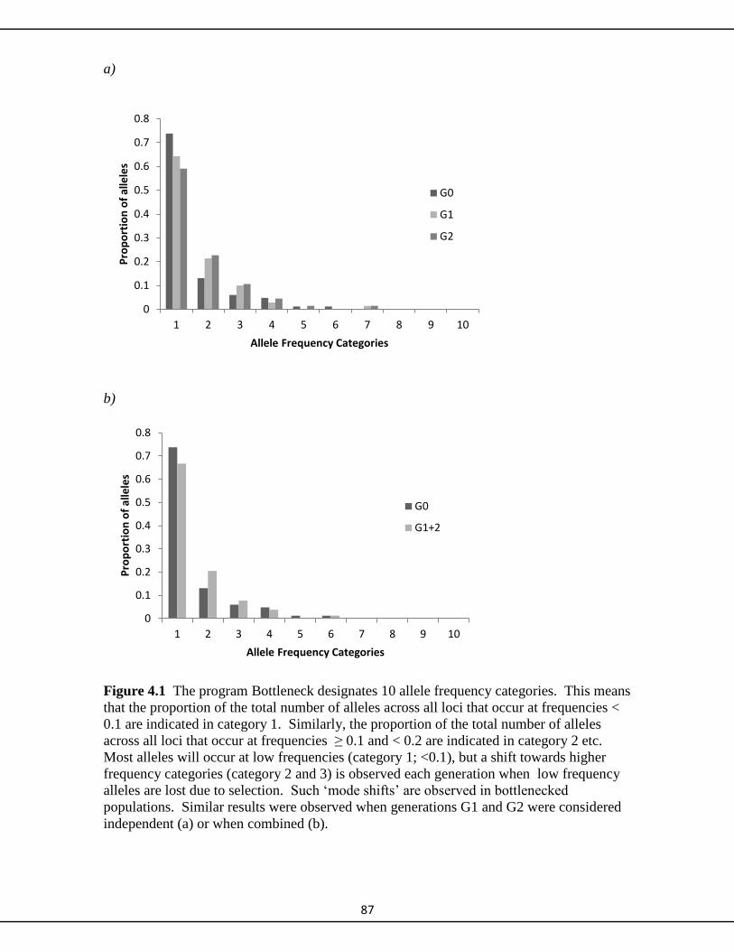
87
a)
b)
Figure 4.1 The program Bottleneck designates 10 allele frequency categories. This means
that the proportion of the total number of alleles across all loci that occur at frequencies <
0.1 are indicated in category 1. Similarly, the proportion of the total number of alleles
across all loci that occur at frequencies ≥ 0.1 and < 0.2 are indicated in category 2 etc.
Most alleles will occur at low frequencies (category 1; <0.1), but a shift towards higher
frequency categories (category 2 and 3) is observed each generation when low frequency
alleles are lost due to selection. Such ‘mode shifts’ are observed in bottlenecked
populations. Similar results were observed when generations G1 and G2 were considered
independent (a) or when combined (b).
0
0.1
0.2
0.3
0.4
0.5
0.6
0.7
0.8
1 2 3 4 5 6 7 8 9 10
Pro
po
rtio
n o
f al
lele
s
Allele Frequency Categories
G0
G1+2
0
0.1
0.2
0.3
0.4
0.5
0.6
0.7
0.8
1 2 3 4 5 6 7 8 9 10
Pro
po
rtio
n o
f al
lele
s
Allele Frequency Categories
G0
G1
G2
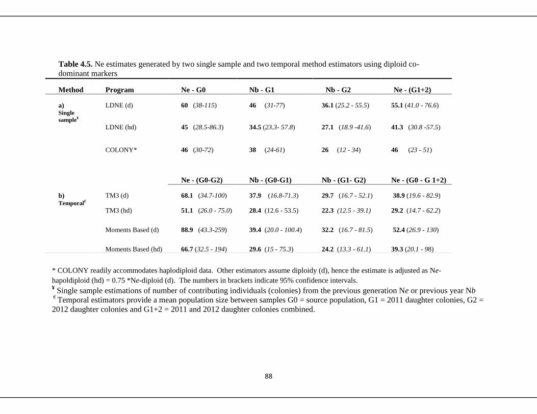
88
* COLONY readily accommodates haplodiploid data. Other estimators assume diploidy (d), hence the estimate is adjusted as Ne-
hapoldiploid (hd) = 0.75 *Ne-diploid (d). The numbers in brackets indicate 95% confidence intervals. ¥ Single sample estimations of number of contributing individuals (colonies) from the previous generation Ne or previous year Nb
€ Temporal estimators provide a mean population size between samples G0 = source population, G1 = 2011 daughter colonies, G2 =
2012 daughter colonies and G1+2 = 2011 and 2012 daughter colonies combined.
Table 4.5. Ne estimates generated by two single sample and two temporal method estimators using diploid co-
dominant markers
Method Program Ne - G0 Nb - G1 Nb - G2 Ne - (G1+2)
a) LDNE (d) 60 (38-115) 46 (31-77) 36.1 (25.2 - 55.5) 55.1 (41.0 - 76.6) Single
sample¥
LDNE (hd) 45 (28.5-86.3) 34.5 (23.3- 57.8) 27.1 (18.9 -41.6) 41.3 (30.8 -57.5)
COLONY* 46 (30-72) 38 (24-61) 26 (12 - 34) 46 (23 - 51)
Ne - (G0-G2) Nb - (G0-G1) Nb - (G1- G2) Ne - (G0 - G 1+2)
b) TM3 (d) 68.1 (34.7-100) 37.9 (16.8-71.3) 29.7 (16.7 - 52.1) 38.9 (19.6 - 82.9) Temporal€
TM3 (hd) 51.1 (26.0 - 75.0) 28.4 (12.6 - 53.5) 22.3 (12.5 - 39.1) 29.2 (14.7 - 62.2)
Moments Based (d) 88.9 (43.3-259) 39.4 (20.0 - 100.4) 32.2 (16.7 - 81.5) 52.4 (26.9 - 130)
Moments Based (hd) 66.7 (32.5 - 194) 29.6 (15 - 75.3) 24.2 (13.3 - 61.1) 39.3 (20.1 - 98)

89
4.4.4 Assessing Effective Population Size (Ne)
4.4.4a Single sample methods
The program Colony can accommodate single sample diploid (worker) data within a
haplo-diploid context and returned Ne = 46 (Table 4.5a) for my baseline (assumed to be a
random sample of a single generation) samples. LDNE accommodates single sample
diploid data and returned Ne.d (diploid) = 60 or Ne.hd (haplodiploid) = 45 [as Ne.hd= 0.75 Ne.d] for
this baseline sample data set. Colony returned Ne’s of 38 and 26 for the 2011 and 2012
cohort’s respectively, while LDNE returned Ne ’s of 34.5 and 27.1 for these data after
correcting for haplodiploidy (Table 4.5a). Finally, Ne of 46 and 41.3 were determined by
Colony and LDNE respectively after pooling the 2011 and 2012 data as one ‘generation’.
4.4.4b Two sample temporal methods
TM3 returned values of 28.4, 22.3 and 29.2 for sample sets (G0 - G1), (G1- G2), and [G0
– (G1+ G2)] respectively when corrected for haplo-diploidy. Similarly, the same data
combinations using the Moments Based approach gave Ne’s of 29.6, 24.2 and 39.3
respectively (Table 4.5b). Two sample analyses with the programs TM3 and Moments
Based of the baseline (G0) and 2011 (G1) cohort data retuned values of 37.9 and 39.4.
Values of 29.7 and 33.2 were returned when the using the 2011 and 2012 sample datasets.
4.5 Discussion
The test population was genetically diverse. Most of the microsatellite loci were highly
polymorphic, and the csd locus was extremely so. These results were not unexpected, and
I hypothesize that much of this observed diversity originates from the sourcing stock
which is a managed stock of likely mixed genetic heritage. In addition, monitoring
demonstrated how low frequency alleles were lost across generations, and allelic richness
decreased significantly due to the selection pressure applied. There was also relative
congruence among a suite of estimators indicating (as expected) that the effective
population size was decreasing as population level diversity dropped.
Although these data suggest that ample variation is present within this population, broader
genome-wide variation is not necessarily inferred since correlations between phenotypic
variation and variation observed at a small number microsatellite markers are generally
weak (Coltman and Slate, 2003). Indeed, these authors suggest that many markers of this
type (~600) are needed to powerfully detect inbreeding on life history traits.
Nevertheless, my observations were encouraging, as it appears that historical management
practices have not diminished variation and adaptive potential in this population. Indeed,
90
the opposite might apply as it is now assumed that managed bee populations might carry
higher levels of genetic diversity than previously thought This new paradigm is based on
research showing that admixture between the two post-expansion (out of Africa)
progenitor lineages in Europe has enhanced the overall diversity of this group (Harpur et
al., 2012). Although my investigation of genome level variation was not extensive, I see
no lack of diversity in this managed population. This conclusion is supported by
sequencing data of putative csd variation (chapter 6).
The WWBBP breeding model developed in part around available resources, and was
tailored to fit into an already established busy commercial beekeeping season. Since the
program suffered severe losses over the 2010/11 winter, approximately 110 replacement
colonies were raised. Approximately 8 effective breeders were selected from the
surviving colonies to contribute to this cohort. Only 60 replacement colonies were
successfully raised in 2012, and queens were raised from only four breeders (effective
number was 3.5) selected from the 2011 survivors. The drone producing colonies were
derived from the remainder of the previous year’s queens, and from older breeder
colonies. Drones from field apiaries might also contribute as no effort is made to remove
then when mating nucleus colonies (glossary) are being constructed in the field. Drones
from production colonies are brought back to the mating apiary where they could mate
with the test queens. What genetic effect could monitoring detect to date, and what clues
might these results provide concerning the long term sustainability of this population if the
breeding strategy was maintained?
There was an obvious and significant decline in allelic richness (loss of diversity) at both
marker types following the first round of selection. There was a significant difference
between the baseline source ‘generation’ and the first cohort (2011) group in the mean
number of alleles per locus detected. Similar comparisons between the baseline and the
2012 cohort demonstrated significant difference in allelic richness, but no significant
difference was indicated between 2011 and 2012.
Allelic richness was also significantly lower when the data from the two cohorts were
combined and compared to the source. These data seems to indicate that the initial round
of breeder selection reduced allelic richness in the 2nd
generation. Honeybees have
overlapping generations and combining the separate cohort data might better represent a
single generation frequency distribution. The resulting dataset should therefore provide a
more compatible sample for comparison with the source population which was assumed to
be a random sample of 2010 and older queens.

91
Analysis of heterozygote excess (HE) in the source population and two cohort groups with
Bottleneck support this interpretation since significant HE was indicated in both the post-
selection cohort groups, but not in the source (2010 and older queens) under the two phase
model (T.M.P), the most appropriate model for microsatellite evolutions used in the
program Bottleneck. This trend was also observed when the cohort groups were
combined. These results are consistent and indicate that a reduction in effective
population size has likely occurred due an imposed bottleneck (selection) event.
I explored the influence of selective breeding on the effective size (Ne) of this managed
honeybee population. Selective breeding potentially limits the transfer of genetic material
across generations, and might therefore result in a reduction in Ne with time. Small
populations also tend to lose genetic diversity more rapidly than population of larger
effective size so that rate of genetic depletion might also accelerate with time. The
combined effects of selection and ever increasing pressures due to reduction in population
size might be of concern in the long term.
There was general congruence between the estimates provided by the programs LDNE and
Colony with both methods indicating a gradual but consistent reduction in population size
with each round of breeding. Single sample estimates such as these generally report the
estimated population size of the previous generation (Hare, 2011), but interpretation of the
results in this case is complicated by the differing composition of the samples. The source
population (G0) was a random sample from a multi-age structured population, while the
G1 and G2 cohorts comprised of daughter queens raised selected set of breeders. I tried to
address this potential issue by combining the G1 (2011) and G2 (2012) daughter cohort
data into a single ‘generation’, which I considered to be two years in this case. A
reduction in Ne was observed using LDNE but not with the program Colony when the
source population was compared to the cohort years combined, although the 95% CI was
smaller in the latter group in both cases. It is also possible that I am overcomplicating
this issue, and that for simplicity’s sake, samples could readily be considered as separate
generations. Although drones from a small number of productive established colonies had
access to cohort queens each year, many of the drone producing colonies were produced
the same time as the breeder colonies now providing the next generation of queens.
Incoming drones picked up during nucleus colony making will likely introduce most
uncertainty into the equation
I therefore also considered G1 and G2 separately as single cohorts, and used LDNE and
Colony to estimate the effective number of parents contributing to each Nb. Four breeders

92
were used to parent G2, so that a minimum Nb of 32 might be expected if each mated with
7 drones (4 queens + 28 drones = 32). This number compares favorably with the single
sample estimates of 27 and 26 determined by LDNE and Colony respectively. Twice as
many breeders contributed to G1, hence the number of contributing parents should be
twice as much as G1 (N = 64). Both Nb estimate generated by LDNE and Colony (34.5
and 38 respectively) were lower than expected.
Temporal method estimates must be interpreted differently, and provide instead
information that is relevant across the temporal period. They also tend to work better for
populations with discrete generations (Wang, 2005). Probabilistic methods have been
shown to have higher accuracy and precision that moments based approaches (Berthier et
al., 2002; Tallmon et al., 2004) which tend to overestimate Ne when genetic drift is strong
(or selection in this case) and when markers with high allelic diversity are used (Wang,
2005). These limitations might explain the higher estimate values generated by the
moment based approach in this study. These methods display greater precision with
increasing temporal separation between samples, and might be handicapped here since
there is not much generational separation between samples. While the accuracy of the
estimates might therefore be questionable, a general decline in population size was again
observed.
No concrete inferences can be made based on these results, partly because the unusual
nature of honeybee genetics complicates the interpretation of Ne estimates for both simple
sample and temporal approaches. Nevertheless, a consistent trend across all methods is
evident. It seems plausible to suggest, particularly if one ignores the potential influence of
overlapping generations, that based on all the genetic evidence presented here, diversity
was eroded across generations and that the effective population size was trending down
with each round of selection.
Genetic monitoring revealed two main points. First, the source population displayed high
levels of genetic diversity at microsatellite loci, and at the hyper-variable region of the csd
locus. From a practical perspective, this diversity suggests that the population might hold
adaptive potential, that can be targeted by selection Secondly, the current selection regime
seems to be an eroding force on this diversity. Results indicate that low frequency alleles
are being lost, and the effective population size is diminishing, but it is not clear if the
current rate of genetic depletion significantly dampens the adaptive potential of this
population. In the next chapter, I investigated the potential short term consequences of this
selection regime by modelling changes across five generations.
93
Chapter 5
Monte Carlo simulation-modelling the influence of
various breeding parameters

94
5.1 Introduction
Predicting the genetic (and hence in part the phenotypic) consequences of selective
breeding in a population of honeybees is complicated by the nature of haplodiploid
genetics, and by the multiple mating behaviour of queens. In order to better understand
the processes involved, honeybee researchers have used computer simulations to model
different closed population breeding scenarios (Page and Laidlaw, 1982a, 1982b; Page
and Marks, 1982; Moritz, 1984, 1986; Omholt and Ådnöy, 1996; Gupta et al., 2012).
Page and Marks (1982) and Page and Laidlaw (1982a, 1982b) were the first to use
computer simulation models to investigate the effects of random mating in a closed
haplodiploid population. They specifically investigated the effects of inbreeding and drift
on the population genetics of sex alleles in genetically isolated artificial populations that
were maintained by instrumental insemination (II). By altering their selection criteria and
population sizes, they used their simulation model to estimate the rate of decay in brood
viability due loss of sex alleles over 40 generations.
Selection and inbreeding not only affects the sex locus, but will also reduce fitness due to
inbreeding depression. Moritz (1984) developed a mathematical model relating
inbreeding depression (quantified as an inbreeding coefficient) to population size, and
illustrated how inbreeding effects depend upon the number of queens selected each year,
and on the number of generations since selection started. This theoretical study also
estimated genetic progress by using published data from ‘real’ populations, and illustrates
how different maximum improvement limits exist for populations of different sizes.
Smaller populations will have lower maximum improvement limits (reduced adaptive
potential), and take fewer generations of selection to reach them.
Simulations have also been used to compare the effects of different selection methods.
Moritz (1986) and Omholt and Ådnöy (1996) compared within-family selection (selecting
the daughter queen with the highest phenotypic value for each breeder queen) and mass
selection (selecting the new breeder queens ignoring familial relationships designs), and
concluded that under most circumstances, mass selection provides the greatest
improvement, although it may be wise to select from within families when population size
is small, and when inbreeding is more of a concern (Moritz, 1986).
A universal assumption made by these closed population simulations, and one that may
not apply in practice (discussed below), is that each generation of test daughter queens
mate only with drones produced by the same group of breeder mothers, and that the
semen from all the selected breeder drones can be pooled and homogenized before being
95
used to inseminate the test queen population. In this way, the models simulate population
situations where Instrumental Insemination (II) is used to maintain isolation. They also
run simulations for up to forty generations with earlier studies using relatively low
numbers of iterations (20-100). Few breeding programs last this long, so that information
on contemporary scale is lacking. All these simulations generally assume relatively large
population sizes, with number of breeders selected each generation ranging from 10-50,
though Moritz (1986) did run simulations comparing a range of breeder numbers ranging
from a low of 1 to a high of 50, and mathematically modelled the effects of inbreeding on
genetic improvement over 40 generations selecting 2-19 breeders each generation.
Maximum character improvement was much lower and is reached more quickly when
lower breeders numbers are used.
5.1.1 My model designs
These models were designed to provide practical guidance for small scale breeding
programs wanting to improve stock quality through open mating and adaptive selection.
The basic model structure assumes a single closed population from which a determined
number of breeder queens are selected each generation. A specified number of daughter
colonies are then raised from these breeders each year and these in turn provide breeders
and drones for the next generation. The methodology here deviates from the closed
population modelling structure applied by earlier research (described above), and does so
to better simulate the approach adopted by the West Wales Bee Breeding Program
(WWBBP). Here, drones from all daughter colonies raised the previous year can
contribute to the next generation.
I developed simulation models in MATLAB, using a Monte Carlo sampling approach
(codes in Appendix iii and iv). The Monte Carlo method was originally conceived by
Stan Ulam in 1943, and became widely applied in later years with the advent of
computing technology (Eckhardt, 1987). Monte Carlo simulations can accommodate
multiple variables and repeatedly sample probability distributions to come up with many
possible answers. When repeated frequently enough, the results can provide a level of
confidence or uncertainty about the possible real outcome of the model. I use total allele
frequency variance per locus (sum of the variance of all alleles at a single locus) as a
model indicator to test for differences between parameter variables.
I developed two models to track genetic change due to selection in a closed haplo-diploid
population. The first model simulates population level changes in allele frequencies at

96
selectively neutral co-dominant loci (one locus at a time). It can accommodate up to 12
alleles of specified frequencies, assumes a closed population, and includes a suite of
variable parameters: number of breeders selected each year, number of daughter queens
raised, and mean number of drones that each of these daughter queens mates with. To
accommodate the overlapping nature of honeybee generations (in this managed situation),
the model also assumes that these daughter queens mate randomly with drones from the
previous year’s colonies. The model runs for 5 breeding cycles and simulates changes
due to breeding on a contemporary scale. Simulated results were compared with observed
allele frequency distributions as determined through genetic monitoring. One of the aims
of modelling was to investigate the relative influence of various breeding parameters
(both within the control of, and independent of breeder intervention) on the rate of allele
frequency shifts and genetic depletion, for this specific small scale breeding approach.
Logic dictates that population level diversity will be constricted if only a selected set of
individuals (males and females) taken from the population (of a certain size) is allowed to
reproduce each year. Parameters were adjusted in an effort to optimize the outcome.
From an applied beekeeping and breeding perspective, this means optimizing the input of
effort (the amount of time, effort and money required to select breeders and raise new
colonies) for maximum output gain (maintaining adaptive diversity).
The second simulation examined the influence of selection parameters on the maintenance
of csd diversity within a closed breeding population. Unlike selectively neutral
microsatellites loci, csd experiences balancing selection as alleles of low frequency are
preferred due to a lower probability of being matched (in a homozygote state) by chance
in diploids (Charlesworth, 2004). Homozygotes were therefore continually purged from
this simulation; otherwise it was similar in principal and construction to the neutral
marker model. It models a closed population, assumes random mating, and drone alleles
are generated by queens from the previous year. Input parameters included: number of
new daughter colonies (queens) started per year, and mean number of contributing drones
per queen. The final version accommodates up to 11 alleles of designated frequency, and
the number of breeders selected for each separate round of breeding can be individually
set. In addition, for each breeding cycle, I calculated the probability that alleles identical
by descent would match at random in a diploid individual. For a specific sex allele, this
probability was assumed to equal the product of its frequency in the randomly selected
breeder pool, and its frequency in the drone producer colonies from the previous

97
generation. The ‘probability of homozygosity’ was then simply converted into expected
mean population brood viability as follows:
% brood viability = 1 – (probability of homozygosity)
The reciprocal of the probability of homozygosity (or 1- brood viability at csd) is equal to
the effective number of alleles in the population (Yokoyama and Nei, 1979). The brood
viability output provided by simulation was easily converted to provide an indication of
change in effective number of sex alleles through time. These three population level
parameters are related as homozygosity becomes more likely, and mean brood viability
decreases, if the number of sex alleles carried becomes diminished due chance or
selection.
A number variables were modelled in these simulations (e.g. number of breeder queens,
population size, and number of drones each daughter queen mates with). Of these, I expect
the number of queens used/selected each year to have the greatest bearing on genetic
preservation across generations. In addition, genetic monitoring had indicated that the
WWBBP population was losing diversity under the current breeding protocol. I modelled the
WWBBP’s current protocol, and expected significant increase (indicating loss of genetic
diversity) in allele frequency variances across generations at both neutral markers and at the
csd. In the latter case, I also expected modelling to illustrate that mean brood viability per
colony could not be maintained above 85% in the long term using only four breeders per
year.
5.2 Methods
5.2.1 Microsatellite methodology
Observed source population data gathered at four microsatellite markers (A7, A79, A441,
and Ap43) were entered into the neutral model (Table 5.1). Initial runs simulated the
breeding program protocols that the WWBBP used during the first two selection cycles;
i.e., eight breeders were selected at random from a simulated source population (G0), and
four were selected from the resulting generation (G1). One hundred new queens were
raised each year, and each was assumed to have mated with seven drones. I initially ran
each simulation between 1000 and 5000 times. The higher number of model iterations
took very much longer to run and no significant advantage in precision (difference in
standard deviations) of the results was gained. Simulations were therefore run 1500 times
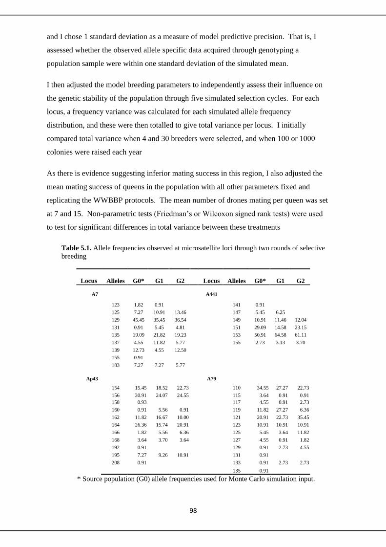
98
and I chose 1 standard deviation as a measure of model predictive precision. That is, I
assessed whether the observed allele specific data acquired through genotyping a
population sample were within one standard deviation of the simulated mean.
I then adjusted the model breeding parameters to independently assess their influence on
the genetic stability of the population through five simulated selection cycles. For each
locus, a frequency variance was calculated for each simulated allele frequency
distribution, and these were then totalled to give total variance per locus. I initially
compared total variance when 4 and 30 breeders were selected, and when 100 or 1000
colonies were raised each year
As there is evidence suggesting inferior mating success in this region, I also adjusted the
mean mating success of queens in the population with all other parameters fixed and
replicating the WWBBP protocols. The mean number of drones mating per queen was set
at 7 and 15. Non-parametric tests (Friedman’s or Wilcoxon signed rank tests) were used
to test for significant differences in total variance between these treatments
Table 5.1. Allele frequencies observed at microsatellite loci through two rounds of selective
breeding
Locus Alleles G0* G1 G2
Locus Alleles G0* G1 G2
A7
A441
123 1.82 0.91 141 0.91
125 7.27 10.91 13.46 147 5.45 6.25
129 45.45 35.45 36.54 149 10.91 11.46 12.04
131 0.91 5.45 4.81 151 29.09 14.58 23.15
135 19.09 21.82 19.23 153 50.91 64.58 61.11
137 4.55 11.82 5.77 155 2.73 3.13 3.70
139 12.73 4.55 12.50
155 0.91
183 7.27 7.27 5.77
Ap43 A79
154 15.45 18.52 22.73 110 34.55 27.27 22.73
156 30.91 24.07 24.55 115 3.64 0.91 0.91 158 0.93 117 4.55 0.91 2.73
160 0.91 5.56 0.91 119 11.82 27.27 6.36
162 11.82 16.67 10.00 121 20.91 22.73 35.45 164 26.36 15.74 20.91 123 10.91 10.91 10.91
166 1.82 5.56 6.36 125 5.45 3.64 11.82
168 3.64 3.70 3.64 127 4.55 0.91 1.82 192 0.91 129 0.91 2.73 4.55
195 7.27 9.26 10.91 131 0.91
208 0.91 133 0.91 2.73 2.73 135 0.91
* Source population (G0) allele frequencies used for Monte Carlo simulation input.
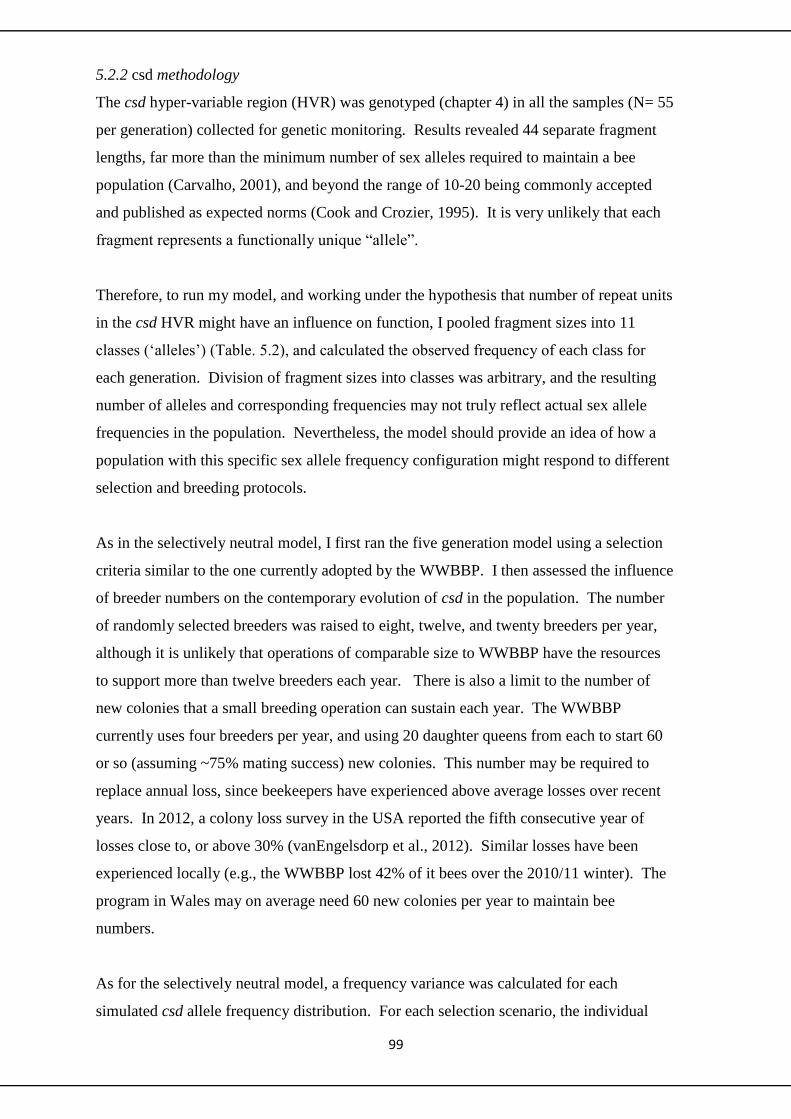
99
5.2.2 csd methodology
The csd hyper-variable region (HVR) was genotyped (chapter 4) in all the samples (N= 55
per generation) collected for genetic monitoring. Results revealed 44 separate fragment
lengths, far more than the minimum number of sex alleles required to maintain a bee
population (Carvalho, 2001), and beyond the range of 10-20 being commonly accepted
and published as expected norms (Cook and Crozier, 1995). It is very unlikely that each
fragment represents a functionally unique “allele”.
Therefore, to run my model, and working under the hypothesis that number of repeat units
in the csd HVR might have an influence on function, I pooled fragment sizes into 11
classes (‘alleles’) (Table. 5.2), and calculated the observed frequency of each class for
each generation. Division of fragment sizes into classes was arbitrary, and the resulting
number of alleles and corresponding frequencies may not truly reflect actual sex allele
frequencies in the population. Nevertheless, the model should provide an idea of how a
population with this specific sex allele frequency configuration might respond to different
selection and breeding protocols.
As in the selectively neutral model, I first ran the five generation model using a selection
criteria similar to the one currently adopted by the WWBBP. I then assessed the influence
of breeder numbers on the contemporary evolution of csd in the population. The number
of randomly selected breeders was raised to eight, twelve, and twenty breeders per year,
although it is unlikely that operations of comparable size to WWBBP have the resources
to support more than twelve breeders each year. There is also a limit to the number of
new colonies that a small breeding operation can sustain each year. The WWBBP
currently uses four breeders per year, and using 20 daughter queens from each to start 60
or so (assuming ~75% mating success) new colonies. This number may be required to
replace annual loss, since beekeepers have experienced above average losses over recent
years. In 2012, a colony loss survey in the USA reported the fifth consecutive year of
losses close to, or above 30% (vanEngelsdorp et al., 2012). Similar losses have been
experienced locally (e.g., the WWBBP lost 42% of it bees over the 2010/11 winter). The
program in Wales may on average need 60 new colonies per year to maintain bee
numbers.
As for the selectively neutral model, a frequency variance was calculated for each
simulated csd allele frequency distribution. For each selection scenario, the individual

100
allele frequency variances were totalled to give ‘total sample variance’ at the csd for each
selection (breeding model) scenario. Total variance was calculated and compared when 4,
8, 12 and 20 breeders were used, and when 100 colonies were raised each year.
5.3 Simulation Results
5.3.1 Microsatellites
The model parameters were initially set to reflect current WWBBP protocols. The
frequency shifts of 38 alleles from four selectively neutral loci (A7, A441, Ap43 and A79)
were simulated and compared to observed allele frequencies after two breeding cycles.
Observed frequencies were within one standard deviation of simulated means in twenty
nine of thirty eight cases (Table 5.3). The simulated median allele frequency value
dropped to below 0 when initial alleles frequency was low (~<0.1). By this measure,
eighteen of the original 38 alleles were potentially lost due to chance as allele frequency
variance increased across selection cycles (Fig 5.1).
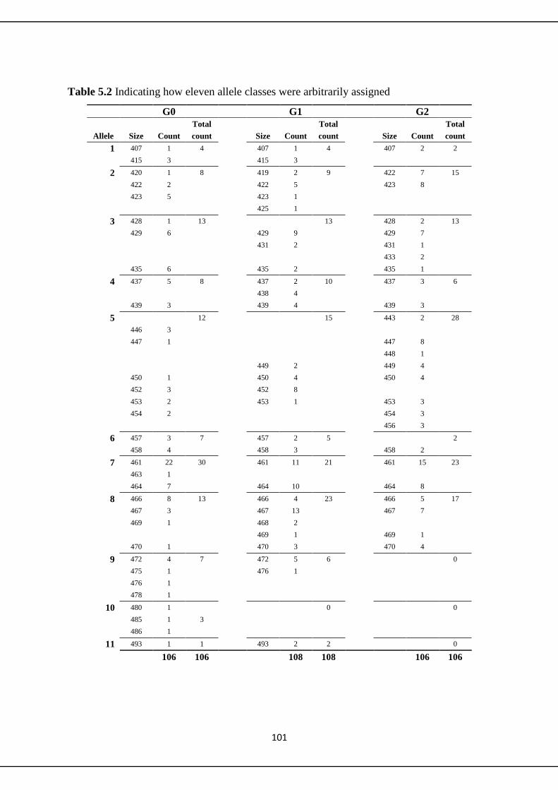
101
Table 5.2 Indicating how eleven allele classes were arbitrarily assigned
G0 G1 G2
Total
Total
Total
Allele Size Count count
Size Count count
Size Count count
1 407 1 4
407 1 4
407 2 2
415 3
415 3
2 420 1 8
419 2 9
422 7 15
422 2
422 5
423 8
423 5
423 1
425 1
3 428 1 13
13
428 2 13
429 6
429 9
429 7
431 2
431 1
433 2
435 6
435 2
435 1
4 437 5 8
437 2 10
437 3 6
438 4
439 3
439 4
439 3
5
12
15
443 2 28
446 3
447 1
447 8
448 1
449 2
449 4
450 1
450 4
450 4
452 3
452 8
453 2
453 1
453 3
454 2
454 3
456 3
6 457 3 7
457 2 5
2
458 4
458 3
458 2
7 461 22 30
461 11 21
461 15 23
463 1
464 7
464 10
464 8
8 466 8 13
466 4 23
466 5 17
467 3
467 13
467 7
469 1
468 2
469 1
469 1
470 1
470 3
470 4
9 472 4 7
472 5 6
0
475 1
476 1
476 1
478 1
10 480 1
0
0
485 1 3
486 1
11 493 1 1 493 2 2 0
106 106
108 108
106 106

102
Table 5.3. Observed vs Simulated allele frequency means at 4 Msat loci
* The simulated frequency was more than 1 standard deviation (based on 1500 iterations) from the
frequency observed in the real population
Locus Allele Observed
Simulated
Mean SD
A79 1 0.227 0.343 0.114*
2 0.009 0.037 0.045
3 0.027 0.047 0.051
4 0.064 0.116 0.073
5 0.355 0.209 0.098*
6 0.109 0.112 0.076
7 0.118 0.055 0.054
8 0.018 0.045 0.048
9 0.046 0.009 0.022
10 0.000 0.009 0.022
11 0.027 0.010 0.024
12 0.000 0.009 0.021
A441 1 0.000 0.009 0.006*
2 0.000 0.055 0.014*
3 0.120 0.109 0.020
4 0.232 0.289 0.028*
5 0.611 0.510 0.031*
6 0.037 0.028 0.010
A7 1 0.000 0.020 0.034
2 0.135 0.075 0.062
3 0.365 0.448 0.118
4 0.048 0.010 0.022*
5 0.192 0.189 0.095
6 0.058 0.047 0.050
7 0.125 0.128 0.080
8 0.000 0.010 0.023
9 0.058 0.074 0.061
Ap43 1 0.227 0.160 0.089
2 0.246 0.305 0.107
3 0.009 0.010 0.024
4 0.100 0.117 0.077
5 0.209 0.262 0.104
6 0.066 0.018 0.032*
7 0.039 0.036 0.043
8 0.000 0.010 0.024
9 0.109 0.071 0.059
10 0.000 0.010 0.024
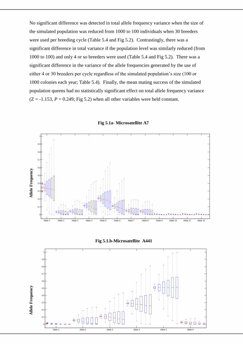
103
Allele 1 Allele 2 Allele 3 Allele 4 Allele 5 Allele 6
0
0.1
0.2
0.3
0.4
0.5
0.6
0.7
0.8
0.9
1
Allele 1 Allele 2 Allele 3 Allele 4 Allele 5 Allele 6 Allele 7 Allele 8 Allele 9 Allele 10 Allele 11 Allele 12
0
0.1
0.2
0.3
0.4
0.5
0.6
0.7
0.8
0.9
1
No significant difference was detected in total allele frequency variance when the size of
the simulated population was reduced from 1000 to 100 individuals when 30 breeders
were used per breeding cycle (Table 5.4 and Fig 5.2). Contrastingly, there was a
significant difference in total variance if the population level was similarly reduced (from
1000 to 100) and only 4 or so breeders were used (Table 5.4 and Fig 5.2). There was a
significant difference in the variance of the allele frequencies generated by the use of
either 4 or 30 breeders per cycle regardless of the simulated population’s size (100 or
1000 colonies each year; Table 5.4). Finally, the mean mating success of the simulated
population queens had no statistically significant effect on total allele frequency variance
(Z = -1.153, P = 0.249; Fig 5.2) when all other variables were held constant.
Fig 5.1a- Microsatellite A7
Fig 5.1.b-Microsatellite A441
A441
All
ele
Fre
qu
ency
A
llel
e F
req
uen
cy
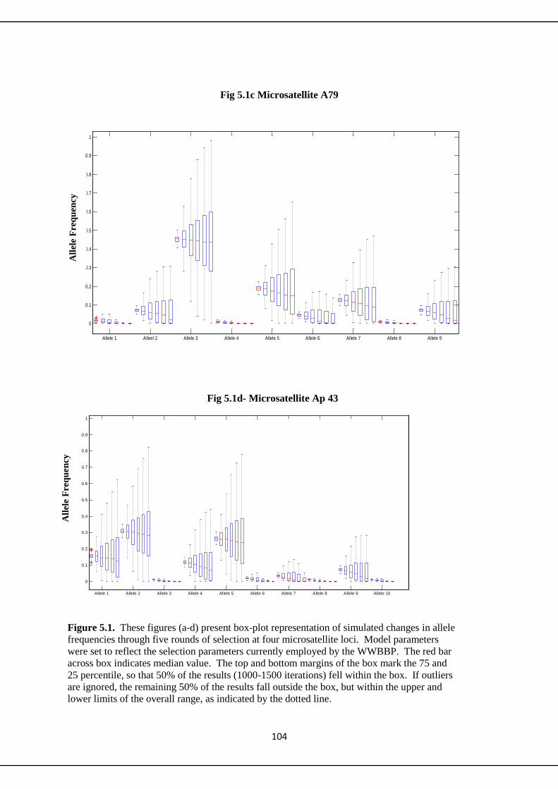
104
Allele 1 Allele 2 Allele 3 Allele 4 Allele 5 Allele 6 Allele 7 Allele 8 Allele 9 Allele 10
0
0.1
0.2
0.3
0.4
0.5
0.6
0.7
0.8
0.9
1
Figure 5.1. These figures (a-d) present box-plot representation of simulated changes in allele
frequencies through five rounds of selection at four microsatellite loci. Model parameters
were set to reflect the selection parameters currently employed by the WWBBP. The red bar
across box indicates median value. The top and bottom margins of the box mark the 75 and
25 percentile, so that 50% of the results (1000-1500 iterations) fell within the box. If outliers
are ignored, the remaining 50% of the results fall outside the box, but within the upper and
lower limits of the overall range, as indicated by the dotted line.
[Type a
quote from
the
document
or the
summary of
an
interesting
point. You
can position
the text box
anywhere
in the
document.
Use the
Allele 1 Alleel 2 Allele 3 Allele 4 Allele 5 Allele 6 Allele 7 Allele 8 Allele 9
0
0.1
0.2
0.3
0.4
0.5
0.6
0.7
0.8
0.9
1
Fig 5.1c Microsatellite A79
Fig 5.1d- Microsatellite Ap 43
All
ele
Fre
qu
ency
A
llel
e F
req
uen
cy

105
5.3.2 Simulating csd (under WWBBP protocols)
Observed allele frequency means for ten of the 11 source population allele classes were
within one standard deviation of simulated means (Fig 5.3a), and eight of the 11 observed
allele frequencies means were within one standard deviation of G1 and G2 simulated
means (Fig.’s 5.3b and 5.3c). Total sample variance increased with each round of
selection (Fig. 5.4) and comparisons using Wilcoxon sign-rank tests indicated statistically
significant differences in allele frequency variance between all paired generations
(breeding cycle) (Z = -2.934, p = 0.003 in all cases). The probability of homozygosity
increased to a maximum of 0.184 after five generations of selection (Fig 5.5) suggesting
that a mean brood viability of 82% could be expected after 5 years. The effective number
of sex alleles decreased from 7.68 to 5.44 over the same 5 cycle period. The simulation
also predicts that several low frequency alleles (~ < 0.05) will be lost from this population
(Fig 5.6). The median allele frequency value (bar across box) dropped below or close to 0
for three low frequency alleles (Alleles 1, 10, and 11). These alleles were lost due to
chance more often than not during simulation runs.
Table 5.4. Table indicating statistical differences in total allele frequency variance at neutral
loci between different simulation treatments
No Daughters Å
No Breeders€
Drones
Z
P-value
Fig 5.3
1000 vs 100 Å
30
7
-1.153
0.249
c and d
1000 vs 100 Å
4 7 -2.210 0.028* a and b
1000 (8)4 vs 30€ 7 -1.992 0.046* a and d
100 (8)4 vs 30€ 7 -2.210 0.028* b and c
100 (8) 4 7 vs 15˚ -1.153 0.249 b and e
Å Tests for statistical difference in total allele frequency variance with daughter population sizes of either 1000
or 100 colonies were conducted when 30 or 4 breeders were used each generation. € The statistical influences of different breeder numbers ((8) 4 and 30) on total frequency variance was tested in
populations of size 100 and 1000 colonies. (8)4 indicate that eight breeders were initially selected from a
source population, and four for each subsequent generation (as implemented by the WWBBP).
*Indicates a statistically significant difference.
˚The potential influence of mean mating success on the total frequency variance under WWBBP protocols was
considered.
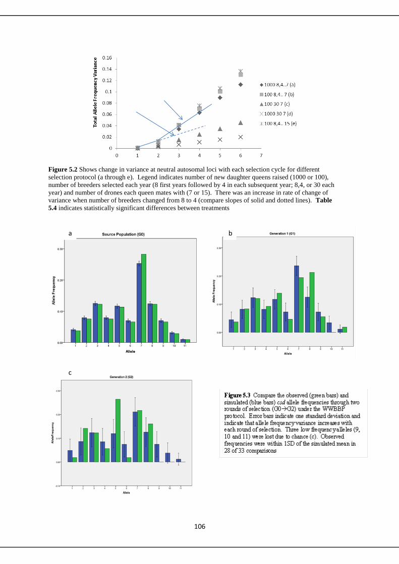
106
Figure 5.2 Shows change in variance at neutral autosomal loci with each selection cycle for different
selection protocol (a through e). Legend indicates number of new daughter queens raised (1000 or 100),
number of breeders selected each year (8 first years followed by 4 in each subsequent year; 8,4, or 30 each
year) and number of drones each queen mates with (7 or 15). There was an increase in rate of change of
variance when number of breeders changed from 8 to 4 (compare slopes of solid and dotted lines). Table
5.4 indicates statistically significant differences between treatments
a b
c
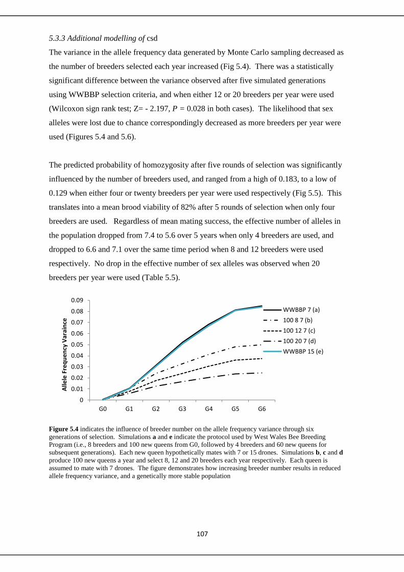
107
5.3.3 Additional modelling of csd
The variance in the allele frequency data generated by Monte Carlo sampling decreased as
the number of breeders selected each year increased (Fig 5.4). There was a statistically
significant difference between the variance observed after five simulated generations
using WWBBP selection criteria, and when either 12 or 20 breeders per year were used
(Wilcoxon sign rank test; Z= - 2.197, P = 0.028 in both cases). The likelihood that sex
alleles were lost due to chance correspondingly decreased as more breeders per year were
used (Figures 5.4 and 5.6).
The predicted probability of homozygosity after five rounds of selection was significantly
influenced by the number of breeders used, and ranged from a high of 0.183, to a low of
0.129 when either four or twenty breeders per year were used respectively (Fig 5.5). This
translates into a mean brood viability of 82% after 5 rounds of selection when only four
breeders are used. Regardless of mean mating success, the effective number of alleles in
the population dropped from 7.4 to 5.6 over 5 years when only 4 breeders are used, and
dropped to 6.6 and 7.1 over the same time period when 8 and 12 breeders were used
respectively. No drop in the effective number of sex alleles was observed when 20
breeders per year were used (Table 5.5).
Figure 5.4 indicates the influence of breeder number on the allele frequency variance through six
generations of selection. Simulations a and e indicate the protocol used by West Wales Bee Breeding
Program (i.e., 8 breeders and 100 new queens from G0, followed by 4 breeders and 60 new queens for
subsequent generations). Each new queen hypothetically mates with 7 or 15 drones. Simulations b, c and d
produce 100 new queens a year and select 8, 12 and 20 breeders each year respectively. Each queen is
assumed to mate with 7 drones. The figure demonstrates how increasing breeder number results in reduced
allele frequency variance, and a genetically more stable population
0
0.01
0.02
0.03
0.04
0.05
0.06
0.07
0.08
0.09
G0 G1 G2 G3 G4 G5 G6
Alle
le F
req
ue
ncy
Var
ain
ce
WWBBP 7 (a)
100 8 7 (b)
100 12 7 (c)
100 20 7 (d)
WWBBP 15 (e)
Figure 5.3a
Figure 5.3b Figure 5.3c
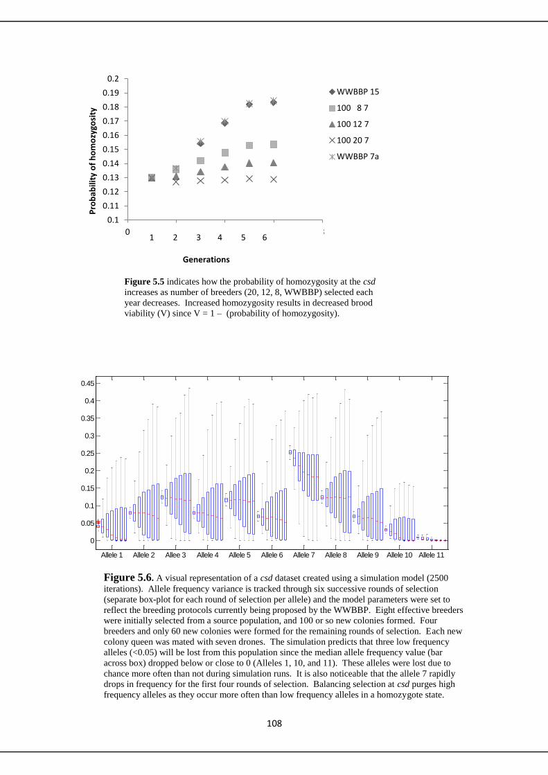
108
Allele 1 Allele 2 Allee 3 Allele 4 Allele 5 Allele 6 Allele 7 Allele 8 Allele 9 Allele 10 Allele 11
0
0.05
0.1
0.15
0.2
0.25
0.3
0.35
0.4
0.45
Figure 5.5 indicates how the probability of homozygosity at the csd
increases as number of breeders (20, 12, 8, WWBBP) selected each
year decreases. Increased homozygosity results in decreased brood
viability (V) since V = 1 – (probability of homozygosity).
Figure 5.6. A visual representation of a csd dataset created using a simulation model (2500
iterations). Allele frequency variance is tracked through six successive rounds of selection
(separate box-plot for each round of selection per allele) and the model parameters were set to
reflect the breeding protocols currently being proposed by the WWBBP. Eight effective breeders
were initially selected from a source population, and 100 or so new colonies formed. Four
breeders and only 60 new colonies were formed for the remaining rounds of selection. Each new
colony queen was mated with seven drones. The simulation predicts that three low frequency
alleles (<0.05) will be lost from this population since the median allele frequency value (bar
across box) dropped below or close to 0 (Alleles 1, 10, and 11). These alleles were lost due to
chance more often than not during simulation runs. It is also noticeable that the allele 7 rapidly
drops in frequency for the first four rounds of selection. Balancing selection at csd purges high
frequency alleles as they occur more often than low frequency alleles in a homozygote state.
0.1
0.11
0.12
0.13
0.14
0.15
0.16
0.17
0.18
0.19
0.2
0 2 4 6 8
Pro
bab
ility
of
ho
mo
zygo
sity
WWBBP 15
100 8 7
100 12 7
100 20 7
WWBBP 7a
1 2 3 4 5 6
Generations

109
Table 5.5 Change in effective number of csd alleles through successive rounds of
selection in relation to number of breeders used
No of Breeders
4 8 12 20
G0 7.69 7.68 7.70 7.70
G1 7.32 7.36 7.63 7.87
G2 6.42 7.05 7.45 7.82
G3 5.88 6.77 7.28 7.79
G4 5.48 6.55 7.13 7.75
G5 5.42 6.51 7.12 7.76
5.4 Discussion
As expected, the number of breeders used each year had the most significant influence
over the rate of loss of genetic diversity. Modelling also supported observed data showing
that low frequency alleles are being lost form the WWBBP population. A significant
increase in total allele frequency variance was observed when the WWBBP protocol was
modelled in simulation trials, suggesting that this population might lose genetic diversity
in the long term when only four breeders per year are used. These results concur with
observed data acquired through genetic monitoring. In addition, modelling of population
level dynamics at the csd (although only hypothetical in nature since actual csd allele
frequencies are unknown) suggested that brood viability could potentially drop to below
85% within five years if current breeding protocols are maintained.
Earlier simulation work on closed population breeding considered various selection
scenarios (e.g. within family, mass, and random), but in each case, only selected breeding
colonies (queens) contributed towards the next generation. They were theoretical in
nature, advocated the use of II, and focused mainly on simulating loss of sex alleles
through time (up to 40 generations). In this study, I model small scale breeding utilizing
open mating, and compare simulated results with real observed data at neutral autosomal
markers. The same breeding/selection model is then applied to the sex locus model,
though the input data used in this case was more theoretical in nature. These models
simulated a small operation utilizing open mating with a contemporary timescale.
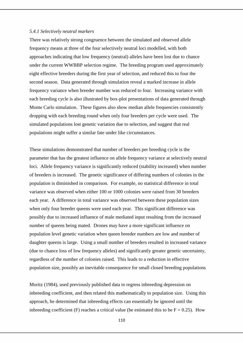
110
5.4.1 Selectively neutral markers
There was relatively strong congruence between the simulated and observed allele
frequency means at three of the four selectively neutral loci modelled, with both
approaches indicating that low frequency (neutral) alleles have been lost due to chance
under the current WWBBP selection regime. The breeding program used approximately
eight effective breeders during the first year of selection, and reduced this to four the
second season. Data generated through simulation reveal a marked increase in allele
frequency variance when breeder number was reduced to four. Increasing variance with
each breeding cycle is also illustrated by box-plot presentations of data generated through
Monte Carlo simulation. These figures also show median allele frequencies consistently
dropping with each breeding round when only four breeders per cycle were used. The
simulated populations lost genetic variation due to selection, and suggest that real
populations might suffer a similar fate under like circumstances.
These simulations demonstrated that number of breeders per breeding cycle is the
parameter that has the greatest influence on allele frequency variance at selectively neutral
loci. Allele frequency variance is significantly reduced (stability increased) when number
of breeders is increased. The genetic significance of differing numbers of colonies in the
population is diminished in comparison. For example, no statistical difference in total
variance was observed when either 100 or 1000 colonies were raised from 30 breeders
each year. A difference in total variance was observed between these population sizes
when only four breeder queens were used each year. This significant difference was
possibly due to increased influence of male mediated input resulting from the increased
number of queens being mated. Drones may have a more significant influence on
population level genetic variation when queen breeder numbers are low and number of
daughter queens is large. Using a small number of breeders resulted in increased variance
(due to chance loss of low frequency alleles) and significantly greater genetic uncertainty,
regardless of the number of colonies raised. This leads to a reduction in effective
population size, possibly an inevitable consequence for small closed breeding populations
Moritz (1984), used previously published data to regress inbreeding depression on
inbreeding coefficient, and then related this mathematically to population size. Using this
approach, he determined that inbreeding effects can essentially be ignored until the
inbreeding coefficient (F) reaches a critical value (he estimated this to be F = 0.25). How

111
rapidly a population reaches this value depends on its size, and is reached earlier in
smaller populations. Moritz estimated that this critical value will be reached in 10 years
when eight new queens each year are selected. However, his model assumed II with each
selected breeder only contributing drones and queens to the next generation. This
scenario differs from the open mating protocols being adopted by the WWBBP. Here,
surviving daughters from the previous generation’s breeder queens contribute most of the
drones, and the current set of selected mother colonies (the breeders) makes no drone
contribution. Nevertheless, both the observed and simulated results indicate that the
genetic diversity is being lost.
Mating success had little effect on population level total allele frequency variance, and
should therefore not significantly affect the genetic makeup of each generation. These
simulations model open mating scenarios in which all drones from the previous year’s
daughter colonies have an equal chance at mating. This aspect of the model reflects the
current approach being adopted by WWBBP, but may not truly reflect the situation in
many breeding operations. Large scale worldwide breeding operations can raise
thousands of queens per week from twenty or so breeders. Most raise daughter queens
from selected colonies for use as drone contributors the following year. This way, the
adaptive transfer of specific desired colony characteristics is mediated through the male
as well as the female line. Isolated mating areas (with apiaries holding mating nuclei with
virgin daughters of selected breeder queens) can then be flooded with these ‘selected’
drones so that breeding is directed from both male and female lines. Such an approach
increases adaptive influence, but might be logistically demanding from smaller scale
operations. Aiding adaptive change through drone influence will be less stringently
controlled in such cases (as with the WWBBP). Allowing virgins uncontrolled access to
drones from any number of successfully overwintered colonies might be a more practical
for small scale breeders. From a breeding perspective, this approach offers limited control
and lacks scientific rigor, but is advocated as a more holistic approach by some
commercial beekeepers since it allows the bees be naturally selected for local adaptation.
The assumption here is that drones from locally adapted queen lines with have a fitness
advantage over drones from less vigorous disease prone lines, so that locally beneficial
traits will be enhanced in the population.
5.4.2 CSD modelling

112
The csd simulation evolved as a progression from the selectively neutral model and was
designed to simulate population level shifts in brood viability resulting from diploid male
production (csd model). This model is complicated by the fact that no diploids can be
homozygous at that locus so that all simulated diploid individuals must to be continually
purged.
It is unclear how my model relates to the actual WWBBP experimental population with
regards to the frequency dynamics of functionally specific csd alleles. Great variation in
fragment length was detected in the HVR, a region thought to possibly confer
functionality at csd. It is unclear how one functional allele differs from another, but based
on these data, it seems unlikely that length is the determining factor. There are estimated
to be 19 or so distinct csd alleles (Adams, 1977), but twice as many HVR fragment
lengths were found in this small population alone. Replication errors might possible lead
to high mutation rates at the repetitive HVR sequences, and variants are maintained over
time by balancing selection acting on functional determining characteristics (e.g. non-
synonymous single nucleotide mutations).
The HVR range in fragment sizes were arbitrarily assigned into the eleven designated
‘allele classes’. Consequently, the frequency distribution entered into the model is purely
hypothetical in nature. Nevertheless, there was relative congruence between simulated
and observed means through two rounds of selection. Both approaches indicated that csd
‘alleles’ at frequencies below 0.05 are vulnerable to loss due to chance under current
WWBBP selection protocols. Observed data (genotyping) indicated that three low
frequency fragment size categories (arbitrary alleles) were lost due to chance after two
rounds of selection.
Simulating progression through an additional three breeding cycles using current
WWBBP protocols shows that the median values for alleles found at frequencies less than
0.1 in the source population, continued to fall with each successive round of selective
breeding. This result suggests that a population with this specific csd allele frequency
distribution would be genetically unstable at this locus for a few years under these
particular selection parameters. Probability of homozygosity at csd increases, and the
effective number of alleles in the population decreases as genetic diversity is lost to
chance. However, there is evidence that an equilibrium state might be achieved within a
few cycles. The rate of change in allele frequency variance decreases after five breeding
113
cycles, and there is a corresponding levelling off in probability of homzygosity and
number of effective alleles in the population
Page and Laidlaw (1985) present simulation data indicating a similar trend. Starting with
a large population, and raising large numbers of colonies each year, they graphed the
probability that brood viability would be greater than 85% against number of generations
for differing numbers of selected queens each year. Ten was the smallest number of
breeders they simulated. In this case, the probability that brood viability would be over
85% rapidly dropped from near 1.0 to 0.2 in five generations. Thereafter the rate of
change declined with each generation. Similar trends are observed for each scenario they
simulated, and in general, selecting more breeders reduced the inevitable decline in brood
viability. They also report that at least 50 breeders must be selected from each generation
to maintain a 95% probability of at least 85% brood viability after 20 generations.
A progression towards an apparent equilibrium state within five generations is similarly
observed in my simulations. As equilibrium is approached, allele frequency variance and
probability of homozygosity decrease as the numbers of breeders used increases. This
trend towards equilibrium is highlighted by the observable shifts in the median allele
frequency values across generations. High frequency allele medians (e.g. allele 7) drop as
homozygotes carrying these alleles are purged from successive generations. Lower
frequency alleles are then favoured and tend to increase in frequency. The model results
reflect balancing selection on the csd locus, and highlight the influence of breeder
numbers on the amount of variation that a population can maintain. Populations can
maintain higher effective numbers of alleles when more breeders are used. This makes
sense as effective population size is defined by number of breeders contributing to next
generation. More breeders result in larger effective population sizes which can maintain
more genetic variation.
5.4.3 Summary/Recommendations
Small bee breeding operations have more control over number of breeders used than any
other breeding parameter. Number of new colonies established each year is limited by
resource availability, and the mean mating success of daughter queens is largely weather
dependent. The WWBBP can generally start no more the 100 new colonies a year in
Wales; they used 4 breeder queens last year, and tried to raise 20 daughter queens from
each one. In addition, mating success may have been sub-optimal over recent years due to

114
persistent and prolonged periods of poor weather. I modelled the various parameters and
adjusted the number of contributing breeder queens to investigate its influence on
population level diversity at both selectively neutral loci and at the csd. The simulations
illustrate that number of breeder queens used is the parameter that has the greatest
influence over the genetic makeup of future generations. Both the observed and the
simulated results suggest that limiting breeder queen number to only four per year results
in genetic depletion over time. Loss of diversity within a contemporary framework was
observed at both selectively neutral loci, and at loci under the influence of selective
forces. This suggests that loss of adaptive potential due to chance loss of adaptively
significant quantitative trait loci could be expected within a contemporary time frame.
There are practical implications for bee-breeders since selecting for adaptive ‘progress’
becomes less effective as population level genetic diversity drops. Consistently and
stringently limiting genetic transfer across generations by using low numbers of breeder
queens will dampen the long term vigour and health of the population. Breeders must
keep this in mind when designing a breeding program.
Sex allele diversity has been a concern for breeders for many years, and particularly for
those working with small populations. My model parameters were hypothetical in terms
of numbers and frequencies of alleles. I modelled eleven alleles in total (an expected
population number) thought the effective number was closer to 8 when accounting for
differential frequencies. There were consistent drops in median allele frequencies at both
the csd and at microsatellite loci when only four breeders were used, and <85% brood
viability brood viability was attained after 5 generations. Median allele frequency
dropped less with eight, and less again with twelve breeders. Median values stabilized
when 20 breeders per year were used, suggesting that the genetic population size would be
sufficiently large to maintain that many alleles over time. From a practical perspective,
this whole debate boils down to one question; how many breeders should be (or can be)
selected? Twenty is more than most want to manage; the results presented in this chapter
suggest that a compromise of between 10-12 breeders may be feasible.
Bee breeders have ultimate control over the number of breeder queens selected each year,
and modelling illustrates that of all possible variables, the number selected has the most
significant influence over the long term genetic stability of a population. Simulations
suggest that the WWBBP could benefit from increasing breeder numbers in order to limit
the loss of low frequency alleles. Increasing the number of breeders (queen lines) would
115
help maintain adaptive potential, and limit the production of diploid drone production due
to homozygosity at the csd in the long term. Evidence suggests that small scale programs
should aim to maintain eight breeding queen lines in order to reduce the likelihood of
rapidly losing diversity due to chance.
116
Chapter 6
Investigating population level csd variation
117
6.1-Introduction
All Hymenoptera (bees, wasps, ants and sawflies) lack sex chromosomes (as seen in
Drosophila) and employ instead a haplo-diploid sex determination system. Sexual
development in this case is directed by a specific region of chromosome 3 (the Sex
Determination Locus - SDL), and specifically, by the complementary sex determination
gene (csd) found within it (Beye et al., 2003). The csd genes translate into atypical forms
of SR- proteins, an important class of gene expression regulators (Long and Caceres,
2009). SR proteins classically have a serine “S” and arginine “R” rich region (RS domain)
and can mediate the splicing of precursor messenger RNA (pre-mRNA) into mRNA (after
cutting out introns). They also typically have RNA binding sites, but these are lacking in
csd (Evans et al., 2004). These SR-type proteins are known to interact with RNA in other
ways (Long and Caceres, 2009). RS domains are frequently involved in protein-protein
interaction, hence it is thought that functionally different csd proteins combine to form an
active RNA splicing product that can activate a downstream response in another gene
within the SDL (fem) to produce female specific mRNA (Gempe et al., 2009). Otherwise,
default male specific fem mRNA is produced. Only individuals that are heterozygous at
csd develop into females.
The csd gene comprises of nine exons distributed across a 9 kb region within the SDL.
These combine to generate a 1.4kb transcript (Heimpel and de Boer, 2008) that contains a
number of regions with distinct amino acid sequence characteristics (Figure 4.1). The
region rich in arginine (R) and serine (S) spans exons 5–7, and a hyper-variable region
(HVR) comprising mostly of asparagine (N) and tyrosine (Y) is located across exons 7 and
8. It is characterized by an {(N)1-4Y}n repeat rich region, and is bordered by a proline-rich
(P) C-terminus (Gempe et al., 2009).
The basis of the difference between functional alleles is not yet understood, but the
repetitive repeat region within the HVR is the prime candidate location for conferring
(Beye et al., 2003; Hasselmann and Beye, 2004; Cho et al., 2006; Gempe et al., 2009) or at
least adding to (Hasselmann et al., 2008) the specificity of alleles. Specificity could be
due to single amino acid differences in the HVR. It is also known that repeat sequence
polymorphism within amino acid coding regions can bestow allele specificity (Fondon and
Garner, 2004), hence specificity might also be conferred by differing numbers of {(N1-
4)Y}x repeats within the HVR. Such amino acid repeat sequences are commonly found
within eukaryotic proteins (Mularoni et al., 2010) and are usually encoded by tri-repeats in

118
regions of high mutation rates that probably result from replication slippage (Mularoni et
al., 2010), or maybe unequal cross-over during recombination. There is also the
possibility that both single amino acid differences and repeat polymorphism work in
combination to confer specificity. A great deal of repeat sequence variation has been
observed at the putatively ‘functional’ HVR, and it is currently thought that different
alleles differ greatly in sequence. Hasselmann and Beye (2004) sampled four Apis
mellifera populations (one each in Germay, South Africa, United States and Brazil) and
detected 15 separate csd lineages, each one differing by 3% in sequence variation.
Around19 different forms of csd are thought to occur in Apis mellifera as a whole (Adams,
1977).
Figure 6.1 The csd gene has nine exons combine to produce a 1.4Kb transcript B. The
hyper-variable region is found in region 3, and area that incorporates exons 6-9. (From Cho et al., 2006)
6.1.1 Implication for breeders
Drones develop from unfertilized eggs and receive their full genetic complement
exclusively from their mother. They are haploid and carry only one copy of the csd gene.
Females in contrast develop from fertilized eggs, but will only do so successfully when the
paternal and maternal csd alleles are different. Individuals developing from eggs fertilized
by sperm carrying functionally identical csd alleles will develop as sexually inviable
diploid (hemizygous) males. Diploid drones constitute a resource drain, and are sacrificed
by colony workers. The population dynamics of csd can influence genetic health at the
individual, colony and population level, and is therefore of imperative importance to the
bee breeder. Genetically depleted populations can have reduced mean colony level brood
viability (less productive) due to increased diploid drone production. Line breeding (in the
strictest sense) is especially prone to genetic depletion as diversity is lost from closed
populations due to chance. It would be of benefit to breeders to monitor csd variation, and
to then use breeder queens of different csd lineages in their program. This cannot be
easily done, since we still don’t definitively know what differentiates one allele from
another.
119
6.1.2 Population screening
I explored three methods to possibly assay a population for csd variation, and assumed in
doing so that the HVR confers allelic specificity. In Chapter 4 I described a method for
screening for HVR size variation, and mention the methodology and results again briefly
below. In this chapter I present HVR population level haploid data. Drones carry only
one copy of the csd gene, and hence provide easy access to allele specific sequences, and a
possible way to monitor population level variation. Finally, I attempted to use denaturing
gradient gel electrophoresis (DGGE) to separate HVR csd fragments amplified in workers.
Diploid derived alleles are most commonly separated by cloning individual allele
fragments into plasmid DNA. The process is time consuming and expensive. DGGE
offers an alternative inexpensive approach to visualize allele specific differences amplified
in diploids, and offers an alternative approach to population screening. The process uses
electrophoresis to separate products based on sequence differences rather than on fragment
size. The goal was to separate fragments so that they could be excised from the gel and
sequenced, but I failed to get sufficient resolution to identify individual fragments
(methods in Appendix v). I therefore attempted improve fragment resolution by running
out the pre DGGE PCR product on low agarose melting gels, and excising the target
product. Unfortunately, too much DNA was lost in the recovery process to warrant
proceeding further. Although I failed to develop a working protocol, the approach does
show promise, and further development work is warranted.
Genotyping previously demonstrated extreme population level fragment length diversity
across the csd HVR. I explored the nature of this variation by sequencing the HVR in
haploid males, and hypothesized that deferring numbers and combinations of (N)1-4Y
repeats would be the most likely source of the observed diversity. I also compared my
sequence results with previously reported data (Hasselmann and Beye, 2004; Cho et al.,
2006; Liu et al., 2011) and used a Neighbour-Joining approach to investigate how local
sequences (i.e. from the WWBBP population) clustered in relation to putative functional
allele sequences derived from individuals that had been sampled from a broad geographic
distribution. I expected that most putative allele sequence lineages to be represented in the
local population.
6.2 Methods
6.2.1 Sequencing haploids
120
Drones were sampled during a single event at a local drone congregation area (situated
900 metres from the mating apiary at Glaspwll) for a related study. It is not clear how
representative such a sample is of actual population diversity, but results should at least
provide an indication of the minimum amount of local variation. Ninety three drones were
sequenced using primer pairs previously used by (Hasselmann et al., 2010) genoRfw 5’-
AGACRATATGAAAAATTACACAATGA-3’, and conscsdrev 5’-
TCATCTCATWTTTCATTATTCAAT-3’. These primers amplified a 750 bp (approx)
fragment of coding and non-coding DNA bridging the HVR (Fig 6.1). Bi-directional
sequencing was initially performed, but as extremely good sequence coverage was
possible sequencing in one direction only, most samples were only sequenced in one
direction.
6.2.2 Definition of csd alleles
Nucleotide sequence alignments were performed with ClustalX version1.8 in Mega5
(Tamura et al., 2007) and alignment results were also adjusted manually for obvious
alignment errors. I also used MEGA5 to compare the drone derived csd sequences using a
Neighbour-Joining (NJ) approach (Saitou and Nei, 1987). The NJ method seemed
appropriate since no phylogenetic inference was intended. In a similar way to Hasselman
and Beye (2004), and Liu et al., (2011) (who investigated possible founder effects by
examining csd region3 variation in an island population of a related species, A. dorsata), a
representative sample from each resulting sequence lineage (cluster) was considered as a
distinct allele and compared to the coding region sequences of previously published
putative alleles (Hasselmann and Beye, 2004). These authors sampled 200–300 embryos
from two to three A. mellifera colonies from four geographical locations: Davis (CA),
Berlin, Stellenbosch (South Africa), and Ribeirão Preto (Brazil). They had a
geographically diverse sample set, and although only a few colonies were sampled, the
samples were expected to be genetically diverse due to polyandry. That is, these samples
carried the genetic contribution of many different fathers (Palmer and Oldroyd, 2001).
The coding regions were determined by consulting the A. mellifera csd gene sequence
reported by Hasselmann and Beye (2004) and Cho et al. (2006), and cDNA sequences of
the A. mellifera csd gene reported by Beye et al. (2003). The coding frame (no stop
codons) was also confirmed using the alignment program CodonCode Aligner. I used
Arlequin (v3.5.1.3; Excoffier and Lischer, 2010) to assess haplotype variability and to
assess degree of gene diversity in the population. This measure is defined as the average

121
number of nucleotide differences per site between any two DNA sequences chosen
randomly from the sample population, and is denoted by π.
I also used NJ to compare haploid derived fragments of known length to see if they
clustered into separate sequence-based lineages. If so, then screening for population level
HVR fragment size variation as determined by genotyping (can use easily sampled
diploids for this) could indicate how much csd variation the population is carrying.
6.2.3 Genotyping
I used genotyping methodology (as described in Chapter 4) to investigated csd-HVR
fragment length polymorphism. A primer pair was developed to target conserved regions
on either side of the HVR, and designed so that fragment lengths would be approximately
450 base pairs (bp) long to facilitate standardizing with the ABI Genescan500 size
standard. The methodology could be applied to both diploid and haploid individuals (see
below), and was used to track genetic change due selective breeding in managed a bee
population.
6.2.4 Sequencing diploids
Worker samples were taken from each of three generations for monitoring purposes, and a
number of individuals were found to carry HVR fragments of equal lengths. These
individuals became the focus of additional attention since a difference in the number of
(N1-4)Y repeats at the HVR (resulting in difference in size) is a proposed mechanism of
conferring csd allele specificity. The detection of csd heterozygous individuals with HVR
fragments of equal lengths could be explained in one of two ways; either the two HVR
‘allele’ sequences were in some way different, or alternatively, if the separate allele
sequences are identical, the HVR performs no functionally specific task during sex
determination. Simply sequencing genomic DNA from ‘homozygous’ (in terms of
fragment size) individuals might shed light on this question
In order to expand sequence coverage either side of the HVR, I then amplified the HVR of
diploids previously determined to have identical fragment lengths using my genotyping
primers (approx.450 bp coverage), with the primer pair used by Hasselman et al., (2010).
These primers provided approximately 750bp of coverage across the region. Constructing
allele specific sequences from heterozygotes using genomic DNA can be problematic
since both alleles will be amplified, and resolving which base goes with which variant

122
problematic. This was not an issue here as I was only interested at this stage in whether
there were sequence differences at the HVR between allele variants, and not in
reconstructing specific allele sequences. I used CodonCode Aligner to align sequences
and preserve coding frame. MEGA5 was also used for aligning noncoding sequence and
for analysing the data.
6.3 Results
Thirty-four different sequence haplotypes were identified from 95 drones sampled at local
congregation areas. Thirty-three distinct haplotypes remained when the HVR was
removed from the analysis. Approximately 750 base pairs of useful sequence were
obtained using single direction sequencing. This amplified fragment comprised of coding
and non-coding regions spanning either side of the csd HVR. The gene diversity per locus
(π), across this whole sequence, was 0.05 ± 0.02, and Neighbour–Joining (NJ) clustering
of sequence data revealed around 20 distinct lineages (Fig 6.2). Very similar clustering
trends were observed when the HVR (region with multiple gaps) was removed from the
analysis. Representative samples from each lineage were aligned at the csd-HVR region
(Fig 6. 3). The HVR coding regions ranged in size from 69 to 90 amino acid residues and
demonstrated comparable variation to those published by Hasselman and Beye (2004) (Fig
6.4).
Genotyping revealed twelve diploid workers carrying HVR ‘alleles’ of equal lengths.
Sequences were found to be different between alleles in all cases and markedly so in
eleven of the twelve cases (sequence electropherograms were unintelligible in these cases).
Contrastingly, one individual (esg3312) carried two very similar coding region sequences
at the HVR. Only six single base pair differences were observed across the 454 bases
spanning the HVR coding region. Three of these differences were synonymous, and two
of the remaining three non-synonymous trasversions were located within the HVR (Figure
6.4). One of these single nucleotide substitutions (G<->T) was located in RS domain and
resulted in a Threonine (T) to Arginine (R) amino acid mutation at position 302 (Cho et
al., 2006). Of all the haploid individuals sequenced (~100), this R variant was uniquely
observed. The other two mutation were A<-> T trasversions, found within the HVR. The
resulting amino acid sequences had either an Asparagine (N) or Lysine (K) at position 340,
and an N or Tyrosine (Y) at position 347 (Cho et al., 2006).
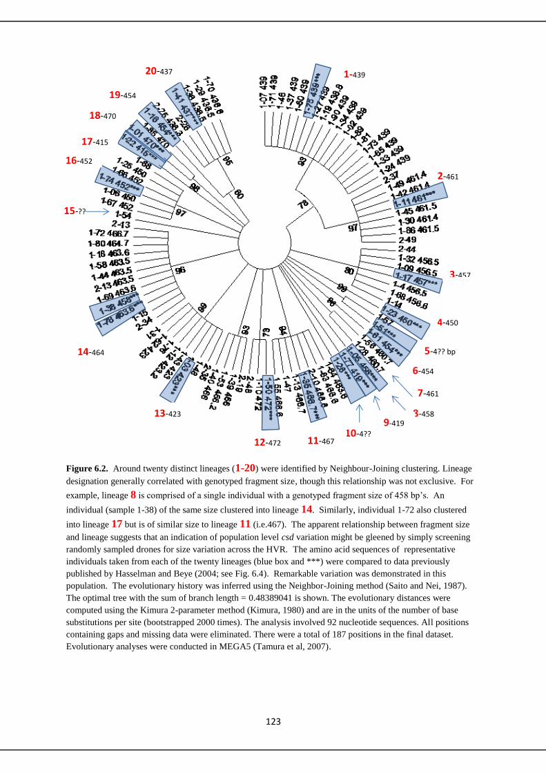
123
Figure 6.2. Around twenty distinct lineages (1-20) were identified by Neighbour-Joining clustering. Lineage
designation generally correlated with genotyped fragment size, though this relationship was not exclusive. For
example, lineage 8 is comprised of a single individual with a genotyped fragment size of 458 bp’s. An
individual (sample 1-38) of the same size clustered into lineage 14. Similarly, individual 1-72 also clustered
into lineage 17 but is of similar size to lineage 11 (i.e.467). The apparent relationship between fragment size
and lineage suggests that an indication of population level csd variation might be gleened by simply screening
randomly sampled drones for size variation across the HVR. The amino acid sequences of representative
individuals taken from each of the twenty lineages (blue box and ***) were compared to data previously
published by Hasselman and Beye (2004; see Fig. 6.4). Remarkable variation was demonstrated in this
population. The evolutionary history was inferred using the Neighbor-Joining method (Saito and Nei, 1987).
The optimal tree with the sum of branch length = 0.48389041 is shown. The evolutionary distances were
computed using the Kimura 2-parameter method (Kimura, 1980) and are in the units of the number of base
substitutions per site (bootstrapped 2000 times). The analysis involved 92 nucleotide sequences. All positions
containing gaps and missing data were eliminated. There were a total of 187 positions in the final dataset.
Evolutionary analyses were conducted in MEGA5 (Tamura et al, 2007).
1-439
2-461
3-457
4-450
5-4?? bp
6-454
bp 7-461
bp 8-458
bp 9-419 10-4??
12-472
13-423
14-464
15-??
16-452
17-415
18-470
1-0
7 4
39
1-7
1 4
39
1-4
6
1-3
7 4
39
1-6
0 4
39
1-7
5 4
39**
*
1-2
7 4
39
1-1
9 4
38.8
1-9
0 4
39
1-34
439
1-02
439
1-89
1-81
1-73 4
39
1-65 4
39
1-33 4
39
1-24 439
93
2-371-49 461.4
1-42 461.4
1-11 461***
1-45 461.5
1-30 461.4
1-86 461.5
2-49
97
78
2-441-32 456.51-09 456.51-17 457***1-4 456.51-68 456.61-14
80
1-23 450***1-571-51***
99
1-61 454***
1-56 460.7
1-28 460.7
96
1-05 458***
1-77 419***
1-2
6***
1-6
4 4
63.6
1-8
3 4
66.6
2-1
0 4
66.6
1-3
5 4
66.7
***
1-1
3 4
66.7
1-4
7
1 5
5 4
66.6
94
1-5
0 4
72***
1-1
0 4
72
2-4
8
73
2-1
9
1-3
9 4
66
1-5
3 4
66.2
1-4
0 4
66
93
2-3
51-4
8 1-03 42
3***1-43 423
1-12 423.21-76
1-62 423
1-31
99
2-341-151-78 463.6***
1-38 458***1-69 463.62-13 463.51-44 463.51-58 463.51-18 463.61-80 464.7
1-72 466.7
2-13
96
1-54
1-67 452
1-06 450
1-74 452***
1-66 452
1-25 4501-88
97
1-22 415***
1-01 470***
1-85 470
98
1-16 454***
2-25 436.3
2-261-4
1 4
37***
1-3
6 4
36.5
1-2
9 4
36.5
1-7
0 4
36.6
9560
19-454
20-437
11-467
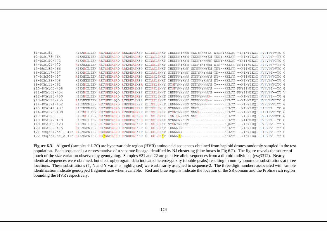
124
#1-DCA151 HIKMRILIEN RETSKERSRD RKEQERSKEP KIISSLSNKT IHNNNNYNNN YNNYNNNYKY NYNNYKKLQY -YNINYIEQI PVPIPVPVYC G
#2-DCA178-464 HIKMKENIEN RETSKERSRD RTERERSREP KIISSLSNKT IHNNNNYKYN YNNNNNNYKN YNNY-KKLYY --NINYIEQI PVPVPV--YY G
#3-DCA150-472 HIKMRILIEN RETSKERSRD RTERERSKEP KIISSLSNKT IHNNNNYKYN YNNNYNNNHY NNNY-KKLQY -YNIINIEQI PVPVPVPIYC G
#4-DCA101-470 RIKMKKNIEN RETSKERSRD RTERERSREP KIISSLSNKT IHNNNNYKYN YNNKYNYNNN NYN--KKLYY KNYIINIEQI PVPVPV--YY G
#5-DAC135-466 HIKMRILIEN RETSRERSRD RRERERSKEP KIISSLSNKT IHNNNNYKNY NNYNNNNYKN YNY--KKLYY --NIINIEQI PVPVPVPVYC G
#6-DCA117-457 HIKMRILIEN RETSKERSRD RTERERSKEP KIISSLSNNY NYNNNNYNNY NNNYNNYNNN YN---KKLYY --NINYIEQI PVPVPI--YC G
#7-DCA204-457 RIKMKILIEN RETSKERSRD RTERERSREP KIISSLSNKT IHNNNNYNNN NYNNYNNNYN NY---KKLYY --NIINIEQI PVPVPVPIYC G
#8-DCA138-458 HIKMKENIEN RETSKERSRD RTERERSREP KIISSLSNKT IHNNNNYKYN YNNNNYKNYN NY---KKLYY --NINYIEQI PVPVPV--YY G
#9-DCA111-461 HIKMRILIEN RETSRERSRD RTERERSKER KIISSLSNNY NYSNYNNYNN NNNYNNNNYN Y----KKLYY --NINYIEQI PVPVPVPIYC G
#10-DCA105-458 HIKMRILIEN RETSKERSRD RKERERSKEP KIISSLSNNY KYSNYNNYNN YNNNNYNNYN -----KKLYY KNYIINIEQI PVPVPI--YC G
#11-DCA161-454 HIKMRILIEN RETSKERSQD RTERERSKEP KIISSLSNNT IHNNNYKYNY NNNNYNNNYN -----KKLYY KNYIINIEQI PVPVPV--YY V
#12-DCA123-450 HIKMRILIEN RETSKERSRD RTERERSREP KIISSLSNKT IHNNNNYKYN YNNNYNNNS- -----KKLYY --NINYIEQI PVPVPI--YC G
#13-DCA116-455 RIKMKENIEN RETSKELSQD RTERETSKEP KIISSLSKNT IHNNNYKYNY NNNNYNNS-- -----KKLYY --NINYIEQI PVPVPVPIYC G
#14-DCA174-452 RIKMKENIEN RETSKERSRD RMERERSKEP KIISSLSNKT IHNNNNYNNN NYNNYNN--- -----KKLYY --NINYIEQI PVPVPVPIYY G
#15-DCA141-437 RIKMKENIEN RETSKERSRD RRERKRSREP KIISSLSNHY NYNNNKYNNY NNDY------ -----KKLYY --NINYIEQI PIPVPI--YC G
#16-DCA175-439 HIKMRILIEN RETSKERSRD RTERERSREP KIISSLSNNY KYSNYNNNNY NNNS------ -----KKLYY --NINYIEQI PIPIPVPIYC G
#17-DCA126- HIKMRILIEN RETSRERSRD RKER-RSKER KIISSLSNNY ISNISNYNNN NNS------- -----KKLYY --NINYIEQI PVPIPVPVYC G
#18-DCA177-419 HIKMKILIEN RETSKERSRD RRERERSKES KIISSLSNNY NYNNCNYKHN ---------- ------KLYY --NIINIEQI PVPVPI--YC G
#19-DCA103-423 RIKMKILIEN RKTSKERSRD RTERERSKEP KIISSLSNNY NYSNYNNNNY ---------- -----KQLCY --NINYIEQI PVPVPV--YY G
#20-DCA122-415 RIKMKENIEN RETSKERSRD RTERERSKEP KIISSLSNNT IHNNNYN--- ---------- -----KKLYY --NINYIEQI PIPVPV--YY G
#21-esg3312he_1-415 RIKMKENIEN RERSKERSRD RTERERSKEP KIISSLSNKT IHNNNNY--- ---------- -----KKLYY --NINYIEQI PIPVPV--YY G
#22-eSg3312he_2-415 RIKMKENIEN RETSKERSRD RTERERSKEP KIISSLSNNT IHNNNYN--- ---------- -----KKLYY --NINYIEQI PIPVPV--YY G
Figure 6.3. Aligned (samples # 1-20) are hypervariable region (HVR) amino acid sequences obtained from haploid drones randomly sampled in the test
population. Each sequence is a representative of a separate lineage identified by NJ clustering (blue boxes in Fig 6.2). The figure reveals the source of
much of the size variation observed by genotyping. Samples #21 and 22 are putative allele sequences from a diploid individual (esg3312). Nearly
identical sequences were obtained, but electropherogram data indicated heterozygozity (double peaks) resulting in non-synonomous substitutions at three
locations. These substitutions (T, N and Y variants highlighted) were arbitrarily assigned to sequence 2. The three digit numbers associated with sample
identification indicate genotyped fragment size when available. Red and blue regions indicate the location of the SR domain and the Proline rich region
bounding the HVR respectively.

125
#1 B1-4 EPKIIS---S LSNKTIHNNN NYKYNYNNNN YNNNNYNNNY NNNCKKL-YY N--IINIEQ- --P
#2 DCA151- EPKIIS---S LSNKTIHNNN NYNNNYNNYN NNYKYNYNNY ----KKLQYY N--INYIEQI PVP
#3 DCA178-463.6 EPKIIS---S LSNKTIHNNN NYKYNYNNNN NNYKNYNNY- ----KKL-YY N--INYIEQI PVP
#4 DCA101-470 EPKIIS---S LSNKTIHNNN NYKYNYNNKY NYNNNNYN-- ----KKL-YY KNYIINIEQI PVP
#5 DCA135-466.7 EPKIIS---S LSNKTIHNNN NYKNYNNYNN NNYKNYNY-- ----KKL-YY N--IINIEQI PVP
#6 DCA204-456.5 EPKIIS---S LSNKTIHNNN NYNNNNYNNY NNNYNNY--- ----KKL-YY N--IINIEQI PVP
#7 DCA138-458 EPKIIS---S LSNKTIHNNN NYKYNYNNNN YKNYNNY--- ----KKL-YY N--INYIEQI PVP
#8 DCA123-449.5 EPKIIS---S LSNKTIHNNN NYKYNYNNNY NNNS------ ----KKL-YY N--INYIEQI PVP
#9 DCA161-454 EPKIIS---S LSNNTIHNNN -YKYNYNNNN YNNNYN---- ----KKL-YY KNYIINIEQI PVP
#10 DCA116-454.6 EPKIIS---S LSKNTIHNNN -YKYNYNNNN YNNS------ ----KKL-YY N--INYIEQI PVP
#11 DCA174-452 EPKIIS---S LSNKTIHNNN NYNNNNYNNY NN-------- ----KKL-YY N--INYIEQI PVP
#12 DCA122-415 EPKIIS---S LSNNTIHNNN YN-------- ---------- ----KKL-YY N--INYIEQI PIP
#13 esg3312_seq1 415 EPKIIS---S LSNKTIHNNN NY-------- ---------- ----KKL-YY N--INYIEQI PIP
#14 esg3312_seq2 415 EPKIIS---S LSNNTIHNNN YN-------- ---------- ----KKL-YY N--INYIEQI PIP
#15 S7-58 EPKIIS---S LSNNTIHNNN YN-------- ---------- ----KKL-YY N--IINIEQ- --P
#16 B2-25 EPKIIS---S LLNNTIHNNN NY-------- ---------- ----KKL-QY YN-INYIEQ- --P
#17 A1-18 EPKIIS---S LSNKTIHNNN NYNNYNN--- ---------- ----KKL-YY N--INYIEQ- --P
#18 A-58 EPKIIS---S LSLKTIHNNN NYKNYN---- ---------- ----KKL-YY N--IINIEQ- --P
#19 DCA126- ERKIIS---S LSNNYISNIS NYNNNNNS-- ---------- ----KKL-YY N--INYIEQI PVP
#20 DCA111-461.3 ERKIIS---S LSNNYNYSNY NNYNNNNNYN NNNYNY---- ----KKL-YY N--INYIEQI PVP
#21 DCA117-457 EPKIIS---S LSNNYNYNNN NYNNYNNNYN NYNNNYN--- ----KKL-YY N--INYIEQI PVP
#22 A2-88 EPKIIS---S LSNNYNYNNN NYKYNYNNYN ---------- ----KKL-YY KNYIINIEQ- --P
#23 A1-28 EPKIISNNNS LSNNYNYNNN YNNYNKHNYN ---------- -----KL-YY N--INYIEQ- --P
#24 DCA141-436.7 EPKIIS---S LSNHYNYNNN KYNNYNNDY- ---------- ----KKL-YY N--INYIEQI PIP
#25 DCA177-419 ESKIIS---S LSNNYNYNNC NYKHN----- ---------- -----KL-YY N--IINIEQI PVP
#26 DCA103-423 EPKIIS---S LSNNYNYSNY NNNNY----- ---------- ----KQL-CY N--INYIEQI PVP
#27 D2-38 EPKIIS---S LSNNYNYNNY NNNY------ ---------- ----LPL-HY N--INYIEQ- --P
#28 S2-31 EPKIIS---S LSNNYNYNNY NNNY------ ---------- ----KPL-YY N--IIYIEQ- --P
#29 D1-22 EPKIIS---S LSNNYKYSNY NNYNNYNNNN YNHYN----- ----KKL-YY KNYIINIEQ- --P
#30 S2-33 EPKIIS---S --NNYNYKNY NNNYNS---- ---------- ----KKL-YY N--IINIEQ- --P
#31 D1-18 EPKIIS---S LSNNYKYSNY NNYNNNYNNY NNYNNNYNNN Y----KL-YY N--INYIEQ- --P
#32 DCA105-458 EPKIIS---S LSNNYKYSNY NNYNNYNNNN YNNYN----- ----KKL-YY KNYIINIEQI PVP
#33 DCA175-439 EPKIIS---S LSNNYKYSNY NNNNYNNNS- ---------- ----KKL-YY N--INYIEQI PIP
#34 S7-16 EPKIIS---S LSNSCNYSNN YYNNNNY--- ---------- ----KKL-YN N--INYIEQ- --P
Figure 6.4. Comparing the hypervariable region (HVR) amino acid sequences of representative drones sampled from the WWBBP population (black) with
representative alleles obtained from geographically broad sources previously published by Hasselman and Beye, (2004) (in red). Sequences were
manually aligned and an attempt was made to group similar sequences. No identical matches were found.
126
6.4 Discussion
Sequencing showed that the HVR fragment size variation (revealed by genotyping)
is mostly due to differing combinations and numbers of (N1-4) Y repeats. Substantial
single nucleotide variation was also revealed by sequencing, both within and around
the HVR. Comparisons between representative sequences taken from the WWBBP
population and previously published data sourced from a broad geographic
distribution, suggest that the local population is genetically diverse. Although a
degree of diversity was expected, the extent of these population level observations
are surprising.
This region (exons 6-9) of the csd gene is known to have elevated rates of both
synonymous and non-synonymous differences (Hasselman and Beye, 2004; Cho et
al., 2006). The gene as a whole has been demonstrated to have a level of
polymorphism five to 10 times that of neutral regions, and functionally distinct new
alleles experience positive selection. Heterozygotes have a selective advantage and
low frequency functional alleles are preferentially selected. These are recognized as
the two main forces driving balancing selection at the locus.
Approximately twenty different csd lineages were indicated by Neighbour-Joining
analysis in the WWBBP sample. Clustering trends demonstrate an apparent
correlation between lineage and fragment length, though due to the nature of the data
(nominal and ordinal/nominal?) the relationship was not statistically tested. The
relationship was not exclusive since some fragment lengths (e.g. 466 and 458) were
observed to have quite different sequences and clustered into different lineages.
Nevertheless, fragment size diversity does provide a general indication of lineage
diversity, and possibly of csd allele variation since the HVR is the prime candidate
area thought to convey allele function. Screening fragment size variation in a
representative sample of diploid worker might therefore provide an indication of sex
allele diversity at the population level.
A representative sample was selected from each the above lineages. The csd-HVR
amino acid sequences were compared to each other, and to sequence information
previously published by Hasselman and Beye (2004). The conserved regions on
either side of the HVR repeat region were easily aligned by hand, but phylogenetic
127
comparisons were not meaningful due to sequence gaps and large differences within
the HVR. Nevertheless, visual comparisons suggest that this population is currently
rich in csd diversity. The above mentioned authors had sampled colonies of A.
mellifera from geographically and genetically diverse backgrounds: Davis (CA),
Berlin, Stellenbosch (South Africa), and Ribeirão Preto (Brazil). Comparable
diversity was observed in our single population. These results seem surprising, but
might reflect the mixed nature of and genetic heritage of British managed bees
(Harpur et al., 2012). In addition, this population of bees was primarily sourced over
a number of years from a reputable and knowledgeable breeder who may have
intentionally designed his program to maintain a genetically diverse population of
commercially viable bees.
The diverse genetic background of these bees was revealed by a Neighbour-Joining
analysis of genetic diversity of coding and non-coding sequence around the HVR. I
conducted the analysis with the HVR region both included and excluded, and in both
cases 13 separate lineages (two or more sequences) clustered, and another seven
sequences were independent. These results are again comparable to previously
published work by Hasselman and Beye (2004). They identified 15 separate csd
lineages when comparing variation within the coding region variants of the gene.
Approximately 19 alleles are thought to exist worldwide (Adam 1977).
It is currently unclear how sequence difference translates into functional variation. I
explored the possibility that alleles might differ in number of (N1-4 )Y repeats found
within the HVR by sequencing diploid workers that were identified by genotyping to
have inherited csd fragments of equal lengths from either parent. Adopting a
rudimentary approach, I sequenced genomic DNA, and serendipitously found
evidence that variation within and around the HVR might be of functional
significance. The sequence data from heterozygote individuals were unreadable in
eleven of twelve cases, indicating that the allelic variants inherited from either parent
were significantly different. In contrast, very similar (six nucleotide differences)
sequences were found in one individual, with only three non-synonymous
differences detected. All were in, or around, the HVR. One of these single
nucleotide mutations resulted in an amino acid (T to R) variant in the SR domain.
Such regions are known to direct protein-protein interactions, and could possibly
128
influence the formation of allelic heterodimers. The R site variant occurs at low
frequency as it was detected only in this one individual. The other two non-
synonymous differences were within the HVR.
These data suggest that if the HVR is functionally relevant, then specific alleles do
not need to differ in number of amino acid residues within the HVR. Differences at
a small number of relevant nucleotide locations might be sufficient to release sexual
development out of the default male mode, but the high number of observed
fragment sizes suggests that other forces (number of repeats in conjunction with
specific nucleotide differences) might also drive the specificity of alleles.
From a practical perspective, investigating sequence diversity at the csd revealed
encouraging results. Broad potentially relevant (i.e., functionally discrete lineages)
diversity was indicated by the presence of differing numbers and combinations of
repeats across the HVR. In addition, an apparent relationship between genetic
lineage and size was revealed. This indicates that one could possible screen for
population level csd diversity by investigating the degree of fragment size variation
across the HVR in the population. Although the specific mechanism (and hence the
source DNA sequence) of csd function is undefined, the degree of variation indicated
in this population suggests that likelihood of diploid drone formation should be low.
129
Chapter 7
Final Discussion

130
Final Discussion
One of the aims of this thesis was to assist in the design of a small breeding program,
and although limited by available time, and by difficulties imposed by poor weather,
the results do have value for the purpose of small scale breeders. Results relating to
local queen mating success will be of interest to all beekeepers in the region. Genetic
monitoring of this specific breeding population provided an indication of the amount
of genetic diversity carried by the source population, and monitoring of post selection
generations revealed how these genetic signatures changed through time. Modelling
and simulation work predicted how this population might genetically change through
time if current breeding protocols are maintained. Hopefully, these results will be of
value to beekeepers hoping to establish a breeding program, and provide guidance for
integrating selection and breeding into an existing honey production operation.
7.1 Mating success
I investigated queen mating success at the West Wales Bee Breeding Program
(WWBBP) during the summer of 2010. Although some queens managed to mate
with sufficient numbers of drones (10 was the max), mating success was on average
(7) well below the accepted species mean of 13 pairings per queen. The semen from
ten or so drones is required to fill a queen’s spermatheca to capacity with sperm, so it
appears that approximately half of the WWBBP’s queens were inadequately mated
and may have had a shorter effective laying lifetime as a consequence.
Nevertheless, queens did manage to mate and establish mature colonies in 75% of
cases in 2010. Similar rates of success were observed in 2011 and 2012, even though
weather conditions were poor during both summers, and were particularly bad in
2012. There was variance in the 2010 mating success experiment, but overall the
results suggests that queens (and drones) can usually find sufficiently prolonged
periods of good mating weather. Since there is a heritable component to mating
success, it might be targeted by breeding from locally strong colonies headed by
second year or third year (long-lived) queens. Wales is located towards the northern
limit of the honeybee’s natural distribution and can experience periods of cold wet
weather at any time of the year, and the WWBBP would benefit from bees that
possess the qualities needed to adequately mate under marginal conditions.

131
7.2 Monitoring
7.2.1 Varroa
The WWBBP experienced substantial varroa attributed losses over the 2010/11
winter. Infestation levels were subsequently monitored in newly established colonies
during 2011 and 2012, and a significant increase in mean number of mites was
observed across years. Counts were taken to monitor population-wide seasonal
trends, but also as an indicator of possible tolerance in young colonies. But since
colony mite count is only marginally heritable, and these colonies were yet to fully
mature, the program could benefit from a more rigorous screen. Recently
recommended approaches that might lead to more rapid improvement in tolerance
include testing for above average expression of hygienic behaviour, as well as
identifying colonies with low mite reproduction rates (Fries, 2012). Screening for
hygienic behaviour is demanding of both time and effort (and must be repeated for
consistent results) for the small scale commercial operator to seriously consider. The
latter of these two tests (i.e., lower mite reproduction rates) would provide a better
benefit return, and is simpler and most practical.
Programs intent on directing population adaptation through purposeful selection
should consider screening colonies with second year queens for low rates of mite
population growth. The methodology accounts for differences in initial infestation
between colonies and are applied to mature colonies with actively laying queens only.
Early and late season counts are needed, so that the rate of mite reproduction can be
determined (Büchler et al., 2010; Lee 2010; Fries, 2012). Following
recommendations by Büchler et al. (2010), the first data point is acquired by counting
the natural mite drop (number of mites falling out of the hive) over the first 3-4 weeks
of brood production in the spring (standardized by being carried out during the Salix
bloom). The second data point demands a little more effort, and is acquired by
counting the number of mites infecting a sample of 300 bees taken from the honey
combs in the uppermost box. Since varroa reproduce in honeybee brood cells, counts
are usually determined by taking nurse bees off the brood nest Fries (2012), a
potentially time consuming operation since the queen must first be located and
secured. However, bees from a honey-box are thought to have a more uniform
infestation (Büchler et al., 2010) and can be sampled without having to access the

132
brood and locating the queen. Relatively inexperienced but competent personnel can
perform varroa counts this way. Nevertheless, if counts are taken at strategically
convenient times (e.g., before and after the early summer nectar flows) the approach
should be considered by suitably resourced programs.
7.2.2 Locating the Queen
Locating queens (the hardest part of sampling from the brood-nest) is much easier if
they are marked, but most commercial operation do not go to the trouble of marking
queens destined for production colonies. Young mated queens are easier to find in
small colonies, and can most conveniently be marked during the transition from the
smaller mating hives into full sized colony box. Mature colonies that have
experienced a supercedure or swarming events, both performance relevant data, are
easier to identify if the queen is marked and any new (unmarked) queens must be
marked for the system to practical in the long term. Clearly, such work is an added
management burden for beekeepers, and an efficient record keeping program must be
implemented (and maintained) for maximum benefit. Many European countries offer
small scale breeders federal assistance and support, but this level of organization is
not currently available in the UK. Small scale breeding programs need to be self-
sufficient and allocate their own resources accordingly.
7.2.3 Production and colony strength
Colony strength was estimated by visual assessment using a standardized approach.
Although this method provided only approximate estimates, it allowed colony
strength to be efficiently assessed during a single monitoring event. Digital methods
for assessing the amount of brood on a frame have been developed. These were
considered, but were rejected for the following reasons. It was recommended that all
bees should be shaken off brood-frames for digitalized programs to work. Such
treatment was considered too disruptive and not conducive to colony wellbeing.
Nevertheless, attempts were made to photograph frames in the field with bees still
attached. Attempts were made to standardize methodology, but this proved difficult
in the field setting where colonies were spread out across the moor on wooden pallets.
Studies utilizing digital assessments have used camera tripods and frame holders at
fixed distances (on level ground) to standardize image quality between frames. Each
monitoring sweep would also require approximately 720 images, or 12 images per

133
colony on the heather. The visual method was adopted after a frank cost benefit
analysis.
Colonies of known size gained weight at different rates as they foraged on heather
nectar and pollen in 2011. Conditions allowed for the foraging efficiency of bees
from different colonies to be compared. Analysis revealed no statistical correlation
between colony size (frames of bees) and weight-gained during a nectar flow that
year. These results suggested that there was variance in foraging efficiency, possibly
due to genetic (hence heritable) variation in the population. Conditions were poor on
the heather in 2012 and did not allow for such comparisons. Colonies gained weight
initially (partly due to increased number of hatching adults bees) but colony weights
declined after all available nectar flows ceased. Nevertheless, a number of choice
colonies stood out due to superior size and weight at the end of the season. There
was a statistically significant reduction in the variance of colony size (frames of bees
and amount of brood) between 2011 and 2012 daughter colonies. The 2012 colonies
were also visibly uniform on inspection, with consistent layout of brood nest and
stores. This increased uniformity is likely due to the selective pressures being applied
across generations.
7.3 Genetic monitoring and modelling
Genetic monitoring revealed ample variation at both neutral microsatellite loci, and
within the hyper-variable region of the csd in the source population. Broader
genome-wide variation is not necessarily inferred by these results since correlations
between phenotypic variation, and variation observed at a small number
microsatellite, markers are generally weak. Nevertheless, these observations do
suggest that the Tropical Forest source population might contain adaptive potential,
and should be responsive to selective breeding applied by the WWBBP.
Monitoring also revealed that low frequency alleles were being lost due to chance,
with significant differences in allelic richness being observed between the source
population and subsequent generations. There was also a general consensus among
various effective population size estimators indicating a slight declines in population
size was occurring with each round of breeding. Loss of genetic diversity is an
inevitable consequence of closed population line breeding, but it must be limited

134
since adaptive selection is less effective when diversity low. Maintaining population
level diversity will provide fitness benefits at the colony level since it has been
demonstrated that genetically diverse colonies are more resistant to environmental
and disease related perturbations. It is also known that a genetically diverse work-
force can maintain a more balanced nest environment than a genetically limited
workforce (Jones et al., 2004).
7.4 Breeding
Within family selection has been recommended for programs that can only maintain a
limited number of queen lines, and is the approach currently adopted by the WWBBP
(Moritz, 1986). Approximately 150 colonies are currently maintained and it is
proposed that new colony production will be limited to approximately 60 queens
from 4 breeders each year (12-20 daughter queens per line). My csd model suggested
that a population of this effective size can only maintain 5 to 6 sex (csd) alleles, and
diploid drone production could increase before stabilizing at 17-18% per colony, and
it is possible (depending on the current number and frequency of sex alleles in the
population) that the mean colony brood viability could drop to 85% within 5 years.
It is unlikely that the WWBBP’s bee population will suffer from the effects of genetic
depletion, at least in the short term, but indications are that diversity could become
limiting if current program protocols are maintained. This population might therefore
reach its maximum improvement potential within a relatively short time frame, and
program managers might consider increasing the number of queen lines it maintains
in order to maintain adaptive potential within the population. This might be achieved
by staggering queen lines, so that each line is only bred from every other year. By
staggering this way, it is probably feasible for programs the size of the WWBBP to
maintain eight queen lines in total. Four queen breeders (one each from a different
line) could be selected one year, and the best colony from each of the other four lines
the following year. Staggering breeding lines might allow genetic diversity could be
maintained, and daughter colonies can be monitored for two full seasons (and
winters) before becoming eligible for breeder selection. One disadvantage of this
approach might be that uncontrolled environmental effects could complicate colony
comparisons. All non-breeder colonies will be part of the production population, and
135
will be located in different apiaries and exposed to differing environmental
conditions.
There was a statistically significant difference in allelic richness between the source
population and both the 2011 and 2012 daughter populations, but not between the two
daughter (2011 and 2012) populations. It is possible that genetic differentiation may
have been is dampened by a potentially broader drone contribution in 2012. Two
daughter colony groups were raised in 2012 and each was mated at different locations
and exposed to drones of different sources. Such an approach could possibly be
adopted to limit potential genetic depletion due limiting number of breeders.
However, it would be worth considering the origin of the male contribution as there is
evidence that the difference in drone input could have influenced the temperament of
the 2012 bees.
Bee mating behaviour is inherently uncertain since queens must pair on the wing with
multiple drones (of potentially unknown origin) some distance from the nest. The
process is assumed to be random as little is known about queen mate choice, though
drones from disease resistant colonies might have a breeding advantage due to better
conditioning. Breeders can influence the transfer of desirable traits via male lines by
flooding mating areas with drones mothered by daughters of colonies displaying the
characteristics of choice. The process remains vulnerable to the vagaries of the
weather, and ultimately, breeders have little control over the number or the origin of
the drones their selected queens mate with.
Contrastingly, breeders have complete control over the number and origin of the
queen lines they select, and the number of daughter colonies they establish each year.
Modelling showed that the number of breeders has the most influence over the
change in allele frequency variance, and the change in population genetic diversity
across generations. For breeders employing open mating, breeder selection is the key
component affecting progressive adaptation.
The WWBBP used eight effective breeders, selected from a source population of
approximately 150 colonies in 2011. Approximately 100 daughter colonies were
raised that summer, and the top 30 performing colonies (based on foraging ability,
varroa infestation and temperament), including representatives from each queen line,
were highlighted as potential breeding stock. Four breeders, each from a different

136
queen line, were selected from this stock the following year and 60 or so new
colonies established. Not all breeders had equal representation in the daughter
population, which comprised of two groups grafted from the same four breeders.
These two daughter cohorts were openly mated at different locations and were
subjected to differing drone mediated influences. No significant genetic
differentiation was detected between the colonies mated at different locations in
2012; hence they were pooled for analysis. There was, however, an apparent
difference in the temper of the bees mated at the two locations. The behavioral
difference could possibly be attributed to the expression of different drone-mediated
defense alleles.
7.5 Considerations for breeders
Declining honeybee health has made commercial beekeeping an increasingly labour
intensive occupation. Selectively breeding for local adaptation can be part of the
solution since it can enhance, at the population level, those heritable characteristics
that allow colonies to be productive and disease tolerant under local conditions, thus
reducing the need for supplemental feeding and medication. However, breeding
protocols must be simple to be of practical use to small-scale breeders, and should
provide a timely return (improvement in the population within a few generations) for
invested effort. Breeders must concurrently guard against depleting genetic diversity,
and the resulting detrimental expression of inbreeding effects (such as diploid drone
production). Integrating the logistics of a breeding program into an already busy
honey-production schedule is part of the challenge, and these are further complicated
when production colonies are migrated (to the heather for example). The challenge of
this project was to enhance local suitability while concurrently preserving genetic
diversity and adaptive potential in the simplest most practical way. A major goal of
this project was to develop a transferable template for successful small-scale
breeding. Recognizing that individual businesses must be managed independently,
certain considerations should be universally addressed by all seriously considering
selective breeding. Amount of effort and focus directed to any one will depend on
the specific circumstances.
7.5.1 Consideration for small scale breeders

137
a) Tracking colony/queen performance. Traditionally done using a paper spreadsheet
or sometimes relevant information is written directly onto a hive label. Data is often
transferred onto a computer based system at a later date. Online applications are
becoming increasingly available (Beetight, Hivetrack), and some offer online access
to a personal database via a cellphone application. Whatever the adopted approach,
the process needs to be simple and practical in the field. Regardless, one needs an
organized and disciplined approach. Possibly allocate days for assessing colony
performances only as relevant data can easily go unrecorded during the hustle and
bustle of a regular beekeeping day (e.g. while splitting colonies, removing honey-
crops). This might not be possible as out-yards are frequently widely distributed, and
not frequently visited. The adopted method will depend in part upon the resources
available, and on management style.
b) Marking queens helps to identify colonies that have recently experienced a
supercedure or swarming event. Un-marked queens are easier to find in when
colonies are small. Young mated/laying queens could be most conveniently marked
sometime before her colony expands to full size.
c) Colonies/queen performance should preferably be monitored for a minimum of 2
years (survive 2 winters) before being considered for breeding stock. If selecting for
mite resistance, then monitoring should compare mite reproduction rates among
established colonies (probably during the second season). Mite numbers can still be
knocked down with a soft treatment ((e.g.3.5% oxalic acid) if loads threaten
overwintering survival (generally over 10% infestation), without affecting rate of mite
population growth during the summer season. If resources are limited (e.g. lack of
skilled personnel) and monitoring impractical (same applies in part to a), then select
for tolerance by selecting the healthiest best performing colonies.
d) Genetically depleted populations do not effectively adapt in response to selective
breeding. Protect against genetic depletion by breeding from multiple queen lines.
Models suggest that a closed population can be maintained with minimal loss if 12
breeders are used and a 100 or so new colonies raised each year. Smaller outfits
could probably maintain adequate long term diversity with 8 breeders, as long as
each was from a different queen-line (and possibly stagger so that each line is only
used every other year). Diploid drone production is also more likely to occur in
populations lacking genetic diversity and mean brood viability may drop to
unacceptable levels if too many sex alleles are lost due to chance. Effective
population size depends on the number of breeders (male and female) contributing to
the next generation, and it in turn affects the number of sex-alleles the population can
maintain.
e) Breeders have greater ‘control’ over drone contribution when mating yards are
isolated. One approach might be to use the daughter colonies of the previous year’s
breeders as drone mothers. This way the breeding characteristics of the selected
‘grandmother’ colonies will be propagated through the male (grandson) line.
f) Account for environmental effects by dispersing colonies from each queen specific
line into different locations.
138
7.6 A final thought
Small-scale breeding programs are handicapped by scale. Few can afford to sacrifice
the time and labour, or have the resources necessary to produce and monitor
(performing varroa counts for example) large numbers of colonies. Collaborative
efforts have proven successful, where the burden of maintaining sufficient numbers
of queen lines to offset potential inbreeding effects, and raising sufficient numbers of
new daughter colonies per line to expose desired (and undesired) adaptive
characteristics, is shared. Independent small-scale breeders must also maintain
multiple queen lines to offset inbreeding, but each line will contribute relatively few
daughters (to the next generation) in comparison to that of large scale programs, and
adaptive ‘progress’ will be slower. Key recommendations include:
Pick as many of your best colonies as you can for breeding, and raise as many queens
from each as possible to capture as much adaptive potential as possible.
Use all these daughter colonies as drone produces the following year and consider
screening for low rates of mite reproduction.
To increase number of queen lines maintained, consider breeding from best line
colony each every other year
Don’t let temperamental colonies breed (re-queen if you can), or be drone sources.
7.7 Further work
The honeybee genome sequence was published in 2006 (Whitfield et al., 2006).
Since then, genome level sequencing and screening technologies have continued to
advance. Geneticists now have available powerful tools to investigate genome level
variation among groups of individuals, and these advances offer beneficial
opportunities for breeding. For example, being able to associate specific genetic
signatures (markers) with particular behaviours (phenotypes) would aid marker
assisted selection; that is the selection of breeding individuals based on identifiable
genetic characteristics. Recent research has shown that the honeybee has a small
genome and a high recombination rate, properties that make the use of quantitative
trait loci (QTL’s) particularly suitable for detecting genomic regions with behavioral
significance and influence.
139
Some progress has been made. QTL’s that influence hygienic and defensive
behaviour are now available, though none of this knowledge has yet had much
practical implication. Finding QTL’s or genes influencing other colony level traits
such as honey production and swarming will require additional advanced molecular
and statistical work, as well as large sample sizes to confirm results. It would require
the combined expertise of a well-funded and equipped genetics facility along with a
proficient and sizable beekeeping program with demonstrable variance in the trait of
interest within its bee population. Assisted marker selection in honeybees is still an
emerging field, and our understanding of the process rudimentary. Finding genetic
locations correlating with trait-specific significance would be a start, but much work
would still remain to understand how to effectively proliferate the desired character
through crossbreeding.
Since drone ‘performance’ has little or no tangible influence on desired colony traits,
they have historically received little attention by breeders. Nevertheless, the haploid
state of drones (males) could aid selection in honeybees since it allows for the direct
testing of individual level traits. For example, selecting drones expressing notable
disease (e.g. virus) resistance could help improve tolerance at the colony level.
Testing traits at the colony level is more complicated since queen honeybees mate
with multiple males and the observed characteristics can result from interactions
between a complex mix of genetic backgrounds. This has been a major barrier to
breeding improvement in bees. Consequently, little progress utilizing available
genomic level information of practical significance has yet been made.
Agricultural practices have become increasingly mechanized across the developed
world over recent decades. These developments have challenged honeybees due to
loss of suitably diverse forage, and increased pesticide exposure. Worldwide research
and debate continue about the possible detrimental influences of pesticides on
honeybee health and productivity, and concern is frequently expressed about the
environment in general. From a regional perspective, the topographical nature of the
landscape in North and mid-Wales has limited industrialization. The region could
therefore be a viable control area (in relation to other areas where more mechanized
forms of farming are practiced) for experimental work designed to investigate how
pesticides affect (e.g. neonicotinoids) bees under field conditions.
140
The distribution of Apis mellifera expanded in concert with human expansion out of
Europe during the latter centuries of the last millennium. They thrived in many areas
and colonies can now be found globally within a belt that extends approximately 60°
north and south of the equator. Bees became crucial for the production of
economically important commercial agricultural crops in many regions. However, as
the recent declines due to varroa and associated viruses demonstrate, bees can be
susceptible to novel pest and disease threats. Because of this, regulations have
periodically been implemented to limit the movement of bees across international
borders. The United States has imposed a decade’s long ban restricting the
importation of bees from Europe in response to the catastrophic losses observed in
Britain during the early part of the century. Bees can currently be imported from
Canada and New Zealand only. Australia has restricted imports from all sources
since 2008, but ten choice queens were recently allowed entry from Canada under
strict quarantine (Thistelton, 2013). These queens were sought in efforts to boost
disease resistance and vitality in isolated populations of Australian bees. Similar
concerns have been expressed concerning the limited genetic resources (due to
historical import restrictions) available in North America. In response, fresh genetic
stocks (queens and sperm of A .m. caucasica) have recently been sourced under
quarantine from Turkey and Georgia (Sheppard, 2013).
My studies revealed high levels of genetic and phenotypic variation (possibly due in
part to a mixed genetic heritage) within a small managed population in Wales. By
characterizing and isolating lines with specific colony-level traits, (e.g. good
temperament, production, frugality etc.) this population could provide a genetic
reservoir for other regions in Britain. A broader geographic perspective could also be
considered. Although the importation of live bees from Britain into many countries is
restricted (and likely to remain so) the movement of germplasm (sperm and eggs)
across international borders is possible (Hopkins et al., 2012), and permitted with
certain precautions. The transportation of fertilized eggs is probably preferable since
they are far easier to collect and carry a complete (male and female) genetic package.
Queens can then be raised from eggs selected from chosen colonies at destination.
Small scale European bee-breeding operations (such the WWBBP) could be genetic
reservoirs for global regions suffering declining production and health due to genetic
depletion.
141
Bee breeding could also benefit if we understood how separate csd alleles differ. It is
known that region 3 csd sequences consistently cluster into separate lineages, and each
cluster is currently considered to be a functionally distinct allele class. Using this
approach, Hasselmann et al., (2008) and Yong Liu et al., (2012) report that putatively
neutral variants from the same class of csd sequences had the same repeat structure in
the HVR. Individuals carrying alleles from the same class should therefore develop
into diploid drones. Controlled mating experiments could provide insight into the
appropriateness of this classification measure. For example, by utilizing instrumental
insemination (II), virgin queen of known csd lineage could be singly mated with sperm
taken from a drone carrying a functionally similar csd allele. The matching of
functionally identical alleles would result in a 50% brood viability since half the brood
would develop as diploid drones and would be removed by the colony worker-force.
With time, a concrete picture illustrating of how separate alleles are functionally
related could be constructed.
142
References
Adam, B., (1987). In Breeding the honey-bee; a contribution to the science of bee
breeding; pg 56-65. Published by Northern bee books, Hebden Bridge, UK
Adams, J., Rothman, E.D., Kerr, W.E., and Paulino, Z.L., (1977). Estimating the
number of sex alleles and queen matings from diploid male frequencies in a
population of Apis Mellifera. Genetics, 86: 583-596
Allen, M., and Ball, B., (1996). The incidence and world distribution of the honey bee
viruses. Bee World, 77: 141–162
Allendorf, F., Leary, R.F., Spurell, P., and Wenburg, J.K., (2001). The trouble with
hybrids. Trends in Ecology and Evolution, 16 (11): 613-622
Anderson, E.C., (2005). An efficient Monte Carlo method for estimating Ne from
temporally spaced samples using a coalescent-based likelihood. Genetics, 17:
955-967
Anderson, D.L., and Trueman, J.W.H., (2000). Varroa jacobsoni (Acari;Varroidae) is
more than one species. Experimental and Appied Acarology, 24: 165-189
Anonymous, (1869). Report of the commissioner of agriculture for the year 1868. U.
S. Government Printing Office, Washington, D.C. pg 272-281
Arechavaleta-Velasco, M.E., Hunt, G.J., and Emore, C., (2003). Quantitative trait loci
that influence the expression of guarding and stinging behaviors of individual
honey bees. Behavior genetics, 33(3), 357–64.
Aston, D., (2010). Honey bee winter loss survey for England, 2007-8. Journal for
Apicultural Research and Bee World, 49(1): 111-112
Baer, B., and Schmid-Hempel, P., (1999). Experimental variation in polyandry affects
parasite loads and fitness in a bumblebee. Nature, 397 (6715): 151 –154
Bailey, L., (1964). The 'Isle of Wight disease': the origin and significance of the myth.
BeeWorld, 45:32-37
Baker, A.C., and Schroeder, D.C., (2008). The use of RNA-dependent RNA
polymerase for the taxonomic assignment of Picorna-like viruses (order
Picornavirales) infecting Apis mellifera L. populations. Virology Journal, 5:10
doi:10.1186/1743-422X-5-10
Banby, M.A. el., (1967). Heritability estimates and genetic correlation for brood-
rearing and honey productionin the honeybee. Procedings of the International
Apicutlural Congress (Apimondia), 21: 498.
Beuhne, R., (1910). Bee mortality. Journal of the Department of Agriculture of
Victoria, 7:149-151.

143
Berthier, P., Beaumont, M., Cornuet, J.-M., and Luikart, G., (2002). Likelihood-based
estimation of the effective population size using temporal changes in allele
frequencies: a genealogical approach. Genetics, 160(2): 741–51
Beye, M., Hasselmann, M., Fondrk, M.K., Page, R.E., and Omholt, S.W., (2003). The
gene csd is the primary signal for sexual development in the honeybee and
encodes an SR-type protein. Cell, 114(4), 419–29
Boecking, O., and Drescher, R.W., (1991). Response of Apis mellifera L. colonies
infested with Varroa jacobsoni Oud. Apidologie, 22: 237-241
Büchler, R., Berg, S., and Le Conte, Y., (2010). Breeding for resistance to Varroa
destructor in Europe. Apidologie, 41(3), 393–408. doi:10.1051/apido/2010011
Bullamore, G.W., (1922). Nosema apis and Acarapis (Tarsonemus) woodi in relation
to Isle of Wight disease. Parasitology, 14:53-62
Cale, G.H., and Gowen, J.W., (1956). Heterosis in the honeybee (Apis mellifera L.).
Genetics, 41: 292-303
Carr, E.G., (1918). An unusual disease of honey bees. Journal of Economic
Entomology, 11: 347-351
Carter, M., and Genersch, E., (2008). Molecular characterization of honeybee viruses,
In, Virology and the honeybee, pg 87-113. Aubert, M., Ball, B., Fries, I.,
Moritz, R., Milani, N., and Bernardinelli, I., (Eds.). Published by the European
Commission, Luxembourg: Office for Offi cial Publications of the European
Communities, ISBN 92-79-00586-3
Carvalho, G.A., (2001). The number of sex alleles (CSD) in a bee population and its
practical importance (Hymenoptera: Apidae). Journal of Hymenopteran
Research, 10: 10–15.
Charlesworth, D., (2004). Sex determination: balancing selection in the honey bee.
Current Biology, 14(14): R568–9. doi:10.1016/j.cub.2004.07.014
Cho, S., Huang, Z. Y., Green, D.R., Smith, D. R., and Zhang, J., (2006). Evolution of
the complementary sex-determination gene of honey bees: balancing selection
and trans-species polymorphisms. Genome Research, 16(11), 1366–75.
doi:10.1101/gr.4695306
Claudianos, C., Ranson, H.,. Johnson, R.M., Biswas, S., and Schuler, M.A., et al.,
(2006). Deficit of detoxification enzymes: pesticide sensitivity and
environmental response in the honeybee. Insect Molecular Biology, 15(5):
615–636
Cobey, W.C, Sheppard, W.S., and Tarpy, D.R., (2012). Status of breeding practices
and genetic diversity in domestic U.S honey bees, in Honeybee Colony Health-
Challenges and Sustainable Solutions, pg 25-36. Sammataro, D., and Yoder,

144
F., (Eds.), CRC press, Taylor Francis group, 6000 broken Sound Parkway,
suite 300, Boca Raton FL-33487
Cook, J.M., and Crozier, R.H., (1995). Sex determination and population biology in
the hymenoptera. Trends in Ecology and Evolution, 10(7): 281–286
Collins, A.M., (1979). Genetics of the response of the honeybee to alarm chemical,
isopentyl acetate. Journal of Apicultural Research, 18: 285-291
Collins, A.M., Rinderer, R.E., Harbo, J.R., and Brown, M.A., (1984). Heritabilitites
and correlations for several charactersin the honey bee. Journal of Heredity,
75: 135-140
Cook, J.M., and Crozier, R.H., (1995). Sex dtermination and population biology in the
hymenoptera. Trends in Ecology and Evolution, 10: 281-286
Coltman, D.W., and Slate, J., (2003). Microsatellite measures of inbreeding: a meta-
analysis. Evolution; International Journal of Organic Evolution, 57(5): 971–
983.
Cornuet, J. M., and Luikart, G., (1996). Description and power analysis of two tests
for detecting recent population bottlenecks from allele frequency data.
Genetics, 144(4): 2001–2014
Cox-Foster, D.L., Conlan,
S., and Holmes, E.C., (2007). A metagenomic survey of
microbes in honey bee colony collapse disorder. Science, 318 5848: 283 – 287
Crnokrak, P., and Roff, D., (1999). Inbreeding depression in the wild. Heredity, 83 (Pt
3) 260–270
Cho, S., Huang, Z.-Y., Green, D., Smith, D.R., and Zhang, J., (2006). Evolution of
the complementary sex-determination gene of honey bees: balancing selection
and transpecies polymorphisms. Genome Research, 16: 1366-1375
Darwin, C.R., (1876). The effects of cross and self fertilisation in the vegetable
kingdom. John Murray, Albemarle Street, London.
Delaney, D., Meixner, M.D., Schiff, N.M., and Sheppard, W.S., (2009). Genetic
characterization of commercial honey bee (Hymenoptera: Apidae) populations
in the United States by using mitochondrial and microsatellite markers. Annals
of the Entomological Society of America, 102(4): 666-673
doi:10.1603/008.102.0411
De la Rua, P., Galian, J., Serrano J., and Moritz, R.F.A., (2001). Genetic structure and
distinctness of Apis mellifera L. populations from the Canary Islands.
Molecular Ecology, 10:1733–1742
De la Rua, P., Galian, J., Serrano J., and Moritz, R.F.A., (2002). Microsatellite
analysis of non-migratory colonies of Apis mellifera iberica from south-eastern

145
Spain. Journal of Zoological Systematics and Evolutionary Research, 40: 164–
168
De la Rua, P., Galian, J., Serrano, J., and Moritz, R.F.A., (2003). Genetic structure of
Balearic honeybee populations based on microsatellite polymorphism.
Genetics Selection and Evolution, 35: 339 – 350
de Miranda, J.R., Cordoni, G., and Budge, G., (2010). The acute bee paralysis virus –
Kashmir bee virus – Israeli acute paralysis virus complex. Journal of
Invertebrate Pathology, 103: S30–S47.
de Miranda, J.R., and Genersch, E., (2010). Deformed wing virus. Journal of
Invertebrate Pathology, 103: S48–S61.
Di Rienzo, A., Peterson, A.C., Gmu, J.C., Valdes, A.M, Slatkin, M., et al., (1994).
Mutational processes of simple sequence repeat loci in human populations.
Proceedings of the National Academt of Science, 91: 3166-3170
Eckhardt, R., (1987). Stan Ulam; John van Neumann and the Monte Carlo method.
Los Alamos Science Special Issue, pg. 131-141
Estoup, A., Solignac, M., and Cornuet, J-M., (1994). Precise assessmentof the number
of matings and of relatedness in honey bee colonies. Proceedings of the Royal
Society of London B Biological Science, 258: 1-7
Estoup, A., Garnery, L., Solignac, M., and Cornuet, J.-M., (1995). Microsatellite
variation in honey bee (Apis Mellifera L.) populations: hierarchical genetic
structure and test of the infinite allele and stepwise mutation models.
Genetics, 140: 679-695
Excoffier, L., and Lischer, H.E.L., (2010). Arlequin suite version 3.5: A new series of
programs to perform population genetics analyses under Linux and Windows.
Molecular Ecology Resources, 10: 564-567
Evans, J.D., Shearman, D.C., and Oldroyd, B.P., (2004). Molecular basis of sex
determination in haplodiploids. Trends in Ecology and Evolution, 19(1): 1–3.
doi:10.1016/j.tree.2003.11.001
Fazier, M., Muli, E., Conklin, T., Schmehl, D., and Torto, B., (2009). A scientific note
on Varroa destructor found in east Africa; threat or opportunity. Apidologie,
41: 463-465. DOI: 10.1051/apido/2009073
Faucon, J.P., Mathieu, L., Ribiére, M.A., Martel, A-C., Drajnudel, P., et al., (2002).
Honey bee winter mortality in France in 1999 and 2000. Bee World, 83: 14-23
Felsenstein, J., (1985). Confidence limits on phylogenies: An approach using the
bootstrap. Evolution, 39: 783-791
146
Fondon, J.W., and Garner, H.R., (2004). Molecular origins of rapid and continuous
morphological evolution. Proceedings of the National Academy of Sciences of
the United States of America, 101(52): 18058–63.
doi:10.1073/pnas.0408118101
Finley, J., Camazine, S., and Frazier, M., (1996). The epidemic of honey bee colony
losses during the 1995-1996 season. American Bee Journal, 136: 805-808
Foote, H.L., (1966). The mystery of the disappearing bees. American Bee Journal,
106: 126-127
Franck, P., Garnery, L., Solignac, M., and Cornuet, J.M., (1998). The origin of west
European subspecies of honeybees (Apis mellifera): new insights from
microsatellite and mitochondrial data. Evolution, 52: 1119–1134
Fries, I., Imdorf, A., and Rosenkranz, P., (2006). Survival of mite (Varroa destructor)
infested honey bee (Apis mellifera) colonies in a Nordic climate. Apidologie,
37: 564-570
Fries, I., (2009). Nosema ceranae in European honey bees (Apis mellifera). Journal of
Invertebrate Pathology, 103(1): S73-S79
Fries, I., (2012). Evaluation of varroa mite tolerance in honeybees. In honeybee
colony health: challenges and sustainable solutions, pg 21-24. Sammataro, D.,
and Yoder, F., (Eds.), CRC press, Taylor Francis group, 6000 broken Sound
Parkway, suite 300, Boca Raton FL-33487
Futuyama, D.J., (1998). in Evolutionary Biology 3rd edition pg. 26. Sinauer
Associates, Inc., 23 Plumtree Road P.O., Box 407, Sunderland, MA 01375-
0407 USA
Garnery, L., Cornuet J.M., and Solignac, M., (1992). Evolutionary history of the
honey bee Apis mellifera inferred from mitochondrial DNA analysis.
Molecular Ecology 1: 145–154
Gempe, T., Hasselmann, M., Schiøtt, M., Hause, G., Otte, M., et al., (2009). Sex
determination in honeybees: two separate mechanisms induce and maintain the
female pathway. PLoS biology, 7(10), e1000222.
doi:10.1371/journal.pbio.1000222
Genersch, E., Evans, J., and Fries, I., (2010). Honey bee disease overview. Journal of
Invertebrate Pathology, 103: S2–S4
Gisder, S., Aumeier, P., and Genersch, E., (2009). Deformed wing virus: replication
and viral load in mites (Varroa destructor). Journal of General Virology, 90:
463–467

147
Gramachko, K.P., and Spivak, M., (2003). Differences in olfactory sensitivity and
behavioral responses among honey bees bred for hygienic behavior. Behaviour
and Ecological Sociobiology, 54: 472–479
Goodwin, M., and Von Eaton, C., (2001). Control of varroa; a guide for New Zealand
beekeepers. Published by the Ministry of Agriculture and Forestry ,PO Box
2526, Wellington, New Zealand
Gupta, P., Conrad, T., Spötter, A., Reinsch, N., and Bienefeld, K., (2012). Simulating
a base population in honey bee for molecular genetic studies. Genetics
Selection Evolution, 44: 14-20
Guzman-Novoa, E., Hunt, G. J., Page, R.E., Uribe-Rubio, J.L., Prieto-Merlos, et al.,
(2004). Paternal effects on the defensive behavior of honeybees. The Journal of
Heredity, 96(4): 376–80. doi:10.1093/jhered/esi038
Harbo, J.R., and Rinderer, T.E., (1980). Breeding and Genetics of Honey Bees.
Beekeeping in the United States Agriculure Handbook, 335: 49 – 57
Harbo, J. R., and Harris, J. W., (1999). Heritability in honey bees
(Hymenoptera:Apidae) of characteristics associated with resistance to Varroa
jacobsoni (Mesostigmata: Varroidae). Journal of Economic Entomology, 92:
261–265
Hare, M.P., Nunney, L., Schwartz, M.K., Ruzzante, D.E., Burford, M., et al. (2011).
Understanding and estimating effective population size for practical
application in marine species management. Conservation Biology : the Journal
of the Society for Conservation Biology, 25(3): 438–49. doi:10.1111/j.1523-
1739.2010.01637.x
Harpur, B., Minaei, S., Kent, C.F., and Zayed, A., (2012). Management increases
genetic diversity of honey bees via admixture. Molecular Ecology, 21(18):
4414–21. doi:10.1111/j.1365-294X.2012.05614.x
Hatcher, P., and Battey, N., (2011). In: Biological diversity: expoiters and exploited.
Published by John Wiley and sons, Chichester, West Sussex, PO19 8SQ
Harris, J.W., (2007). Bees with varroa sensitive hygiene preferentially remove mite
infested pupae aged ~ five days post capping. Journal of Apicultural Research
and Bee World, 46(3): 134-139
Hasselmann, M., and Beye, M., (2004). Signatures of selection among sex-
determining alleles of the honey bee. Proceedings of the National Academy of
Sciences of the United States of America, 101(14): 4888–93
doi:10.1073/pnas.0307147101
Hasselmann, M., Gempe, T., Schiøtt, M., Nunes-Silva, C.G., Otte, M., et al., (2008).
Evidence for the evolutionary nascence of a novel sex determination pathway
in honeybees. Nature, 454(7203), 519–522. doi:10.1038/nature07052

148
Hasselmann, M., Lechner, S., Schulte, C., and Beye, M., (2010). Origin of a function
by tandem gene duplication limits the evolutionary capability of its sister copy.
Proceedings of the National Academy of Sciences of the United States of
America, 107(30), 13378–83. doi:10.1073/pnas.1005617107
Heimpel, G.E., and de Boer, J.G., (2008). Sex determination in the hymenoptera.
Annual Review of Entomology, 53, 209–230
doi:10.1146/annurev.ento.53.103106.093441
Higes, M., Martín-Hernández, R., and Meana, A., (2006). Nosema ceranae, a new
microsporidian parasite in honeybees in Europe. Journal of Invertebrate.
Pathology, 92, 81–83
Higes, M., MartínHernández, R., Garrido-Bailón, E., González-Porto, A.V., García-
Palencia, P., et al., (2009). Honeybee colony collapse due to Nosema ceranae
in professional apiaries. Environmental Microbiology Reports, 1(2): 110–113
Highfield, A.C., El Nagar, A., Mackinder, L.C.M., Noel, L., Hall, M.J., et al., (2009).
Deformed wing virus implicated in overwintering honeybee colony losses.
Applied and Environmental Biology, 75(22):7212–7220
Hopkins, B.K., Herr, C., and Sheppard, W.S., (2012). Sequential generations of honey
bee (Apis mellifera) queens produced using cryopreserved semen.
Reproduction Fertility and Development, 24(8): 1079-83. doi:
10.1071/RD11088
Hughes, W.O.H., and Boomsma, J.J., (2004). Genetic diversity and disease resistance
in leaf-cutting ant societies. Evolution, 58(6): 1251-1260
Jaffé, R., Dietemann, V., and Allsopp, M.H., Costa, C., Crewe, R.M., et al., (2010).
Estimating the density of honeybee colonies across their natural range to fill
the gap in pollinator decline censuses. Conservation Biology : the journal of
the Society for Conservation Biology, 24(2): 583–93. doi:10.1111/j.1523-
1739.2009.01331.x
Jensen, A.B., Palmer, K.A., Boomsma, J.J., and Pederson. B.O., (2005). Varying
degrees of Apis mellifera ligustica introgression in protected populations of the
black honeybee, Apis mellifera mellifera, in northwest Europe. Molecular
Ecology, 14: 93-106.
Jones, O.R., and Wang, J., (2010). COLONY: a program for parentage and sibship
inference from multilocus genotype data. Molecular Ecology Resources,
10(3), 551–5. doi:10.1111/j.1755-0998.2009.02787.x
Jones, J.C., Myerscough M.R., Graham S., and Oldroyd, B.P., (2004). Honey bee nest
thermoregulation: diversity promotes stability. Science, 305. No 5682: 402-404
Kauffeld, N.M., Everitt, J.H., and Taylor E.A., (1976). Honey bee problems in the Rio
Grande Valley of Texas. American Bee Journal, 116: 220-222
149
Kimura, M., (1980). A simple method for estimating evolutionary rate of base
substitutions through comparative studies of nucleotide sequences. Journal of
Molecular Evolution, 16: 111-120
Kulinčević, J.M., (1986). Breeding accomplishments with honeybees. In Bee Genetics
and Breeding, Rinderer T.E., (Ed.). Published by Northern Bee Books,
Hebden Brook UK
Kulinčević, J.M., Rothenbuhler, W.C., and Rinderer, T.E., (1982). Disappearing
disease. Part I. Effects of certain protein sources given to honey-bee colonies in
Florida. American Bee Journal, 122: 189-191
Kulinčević, J.M.,. Rothenbuhler, W.C, and Rinderer, T.E., (1984). Disappearing
disease: III. A comparison of seven different stocks of the honey bee (Apis
mellifera). In The Ohio State University, Research Bulletin 1160. Ohio
Agricultural Research and Development Center, Wooster, Ohio, 21 pp
Laidlaw, H.H., (1944). Artificial insemination of the queen bee (Apis mellifera L.)
morphological basis and results. Journal of Morphology, 74: 429-465
Lapidge, K., Oldroyd, B., and Spivak, M., (2002). Seven suggestive quantitative trait
loci influence hygienic behavior of honey bees. Naturwissenschaften, 89: 565–
568
Lagisz, M., Port, G. and Wolff, K., (2010), A cost-effective, simple and high-
throughput method for DNA extraction from insects. Insect Science, 17: 465–
470. doi: 10.1111/j.1744-7917.2010.01318.x
Lande, R., (1988). Genetics and demography in Biological Conservation. Science,
241(4872): 1455-1460
Le Conte, Y., and Navajas, M., (2008). Climate change: impact on honey bee
populations and diseases. Revue Scientifique et Technique de l`Office
International des Epizooties, 27: 499-510
Liautard, C., and Sundström, L., (2005). Estimation of individual level of inbreeding
using relatedness measures in haplodiploids. Insectes Sociaux, 52(4): 323–326
doi:10.1007/s00040-005-0814-0
Long, J.C., and Caceres, J.F., (2009). The SR protein family of splicing factors: master
regulators of gene expression. The Biochemical Journal, 417(1) 15–27
doi:10.1042/BJ20081501
Luikart, G., Allendorf, F.W., Cornuet, J.M., and Sherwin, W.B., (1998). Distortion of
allele frequency distributions provides a test for recent population bottlenecks.
Journal of Heredity, 89(3): 238-48
Luikart, G.R., Tallmon, D.A., Schwartz, M.K., and Allendorf, F.W., (2010).
Estimation of census and effective population sizes: the increasing usefulness
150
of DNA-based approaches. Conservation Genetics, 11(2), 355–373.
doi:10.1007/s10592-010-0050-7
Liu, Z.-Y., Wang, Z.-L., Yan, W.-Y., Wu, X.-B., and Zeng, Z.J., (2012). The sex
determination gene shows no founder effect in the giant honey bee, Apis
dorsata. PLoS one 7(4): e34436. doi:10.1371/journal.pone.0034436
Liu, Z.-Y., Wang, Z.-L., Wu, X.-B., Yan, W.-Y. and Zeng, Z.-J. (2011), csd alleles in
the red dwarf honey bee (Apis florea, Hymenoptera: Apidae) show
exceptionally high nucleotide diversity. Insect Science, 18: 645–651. doi:
10.1111/j.1744-7917.2011.01437.x
Macedo, P.A., and. Ellis, M.D., (2002). Using inert dusts to detect and access Varroa
infestations in honey bee colonies. Journal of Apicultural Research, 40: 3-7
Mackensen, O., (1947). Effect of carbon dioxide on initial ovipostion of artificially
insemination virgin queen bees. Journal of Economic Entomology, 40: 344-
349
Maori, E., Paldi, N., Shafir, S., Kalev, H., Tsur, E. et al., (2009). IAPV, a bee-
affecting virus associated with collapse colony disorder can be silenced by
dsRNA ingestion. Insect Molecular Biology, 18(1): 55–60
Martín-Hernández, R., Meana, A., Prieto, L. Martínez-Salvador, A., Garrido-Bailón,
E., et al., (2009). Outcome of Colonization of Apis mellifera by Nosema
ceranae. Applied and Environmental Microbiology, 73 (20) 6331–6338
Martin, S. J., Highfield, A.C., Brettell, L., Villalobos, E.M., Budge, G.C. et al.,
(2012). Global Honey Bee Viral Landscape Altered by a Parasitic Mite.
Science 336, 1304-1306
Meixner, M. D., Costa, C., and Kryger, P. et al., (2010). Conserving diversity and
vitality for honey bee breeding. Journal of Apicultural Research, 49(1), 85–92
doi:10.3896/IBRA.1.49.1.12
Moretto, G., Gonçalves, L.S., and De Jong, D., (1993). Heritability of Africanized and
European honey bee defensive behaviour against the mite Varroa jacobsoni.
Rev. Bras. Genet. 16: 71-77.
Moritz, R.F.A., (1984). Selection in small populations of honeybees (Apis mellifera
L.) Tierzuchtung Zuchtungsbiologie. l0l: 394-40
Moritz, R.F.A., (1986). Comparison of within and mass selection in honeybee
populations. Journal of Apicultural Research, 25: 146-153

151
Moritz, R.F.A., Hartlte, S., and Neuman, P., (2005). Global invasion of the Western
Honeybee (Apis mellifera) and the consequences for biodiversity. Ecoscience
12 (3): 289-301
Mraz, C., (1977). Disappearing disease south of the border. Gleanings in Bee Culture
105: 198
Mularoni, L., Ledda, A., Toll-Riera, M., and Alba, M.M., (2010). Natural selection
drives the accumulation of amino acid tandem repeats in human proteins.
Genome Research, published online March 24, 2010
doi:10.1101/gr.101261.109
Nei, M., and Tajima, F., (1981). Genetic drift and estimation of effective population
size. Genetics, 98(3): 625–40
Navajas, M., Migeon A., Alaux, C., Martin-Magniette, M.L., Robinson, G.E.et al.,
(2008). Differential gene expression of the honey bee Apis mellifera associated
with Varroa destructor infection. BMC Genomics, 9: 301-11
Navajas, M., (2010). Tracking the colonization history of invasive species Varroa
destructor. In Trends in Acarology Proceedings of the 12th
International
Congress. Sabelis, M.A, and Bruin, J., (Eds). Springer Science Media B.V.
Neumann, P., and Hepburn, R., (2002). Behavioural basis for social parasitism of
Cape honeybees (Apis mellifera capensis). Apidologie, 33: 165–192
Neumann, P., and Carreck, N.L., (2010). Honey bee colony losses. Journal of
Apicultural Research, 49(1): 1-6
Oldroyd, B.P., (2012). Domestication of honey bees was associated with expansion of
genetic diversity. Molecular Ecology, 21(18): 4409 - 4411
Oliver, R., (2012) The Harvard study on neonicotinoids and CCD.
http://scientificbeekeeping.com/the-harvard-study-on-neonicotinoids-and-ccd/
Omholt, S.W., and Ådöny, T., (1996). Effects of various breeding strategies on
diploid drone frequency and quantitative traits in a honey bee population.
Theoretical and Applied Genetics, 89: 687-692
Oertel, E., (1965). Many bee colonies die of an unknown cause. American Bee
Journal, 105: 48-49
Olley, K., (1976). Those disappearing bees. American Bee Journal, 116: 520-521
Oxley, P.R., Spivak, M., and Oldroyd, B.P., (2010). QTLs for hygienic behaviour in
honeybees (Apis mellifera) influence likelihood of engaging in task and
propensity to engage in specific task components. Molecular Ecology, 19:
1452-1461
152
Page, R.E., and Ladlaw, H.E., (1982a). Closed population honbeeyb breeding. l.
population genetics of sex determinarion. Journal of Apicultural Research, 2l
30-37
Page, R.E, and Ladlaw, H.E., (1982b) Closed population honeybeeb breeding. 2.
Comparative methods of stock maintenance and selective breeding. Journal of
Apicultural Research, 2l: 38-44
Page, R.E., and Marks, R.W., (1982). The population genetics of sex determination in
honey bees: random mating in closed populations. Heredit, 48(2): 263-270
Page, R.E., Laidlaw, H.E., (1985). Closed population honeybee breeding program. Bee
World, 66(2): 63-72
Palmer, K., and Oldroyd, B.P., (2001). Mating frequency in Apis florea revisited
(Hymenoptera, Apidae). Insectes Sociaux, 48(1): 40–43
doi:10.1007/PL00001743
Palmer, K., and Oldroyd, B.P., (2003). Evidence for intra-colonial genetic variance in
resistance to American foulbrood of honey bees (Apis mellifera): further
supportfor the parasite/pathogen hypothesis for the evolution of polyandry.
Naturwissenschaften, 90: 265–268
Paxton, R.J., (2010). Does infection by Nosema ceranae cause colony collapse
disorder in honey bees (Apis mellifera)? Journal of Apicultural Research,
49(1): 80-84
Paxton, R.J., Klee, J., Korpela, S., et al., (2007). Nosema ceranae has infected Apis
mellifera in Europe since at least 1998 and may be more virulent than Nosema
Apis. Apidologie, 38: 558-565
Rather, D. Buzzkill on Dan Rather reports. Aired 2nd
April, 2013. http://www.danrather.com/videos/rather-reports.html
Ramadan, M.M., Reimer, N.J., Oishi, D.E., Young, C.L., and Heu, R.A., (2008).
State of Hawaii new pest advisory. Department of Agriculture, No. 07-01
Ribière, M., Lallemand, P., Iscache, A.-L., Schurr, F., Celle, O., et al., (2007). Spread
of infectious chronic bee paralysis virus by honeybee (Apis mellifera L.) feces.
Applied and Environmental Microbioloyg, 73(23): 7711–7716
Ribière, M., Ball, B., and Aubeent, M.F.A., (2008). Natural history and geographical
distribution of honeybee viruses. In, Virology and the honeybee, Pg 26-72.
Aubert, M., Ball, B., Fries, I., Moritz, R., Milani, N., and Bernardinelli, I.,
(Eds.). Published by the European Commission, Luxembourg: Office for
Official Publications of the European Communities, ISBN 92-79-00586-3
Richard, F.J., Tarpy, D.R., and Grozinger, C.M., (2007). Effects of insemination
quantity on honey bee queen physiology. PLoS One, 2(10): e980.
doi:10.1371/journal.pone.0000980.
153
Rinderer, T.E., (1989). In Bee Genetics and Breeding pg. 310. Published by
Northern Bee Books Scout Bottom Farm, Mytholmroyd, Hebden Bridge
HX7 5JS (U.K.)
Rinderer, T.E., Guzman, L.I., Harris, J.W., Kuznetsov, V., Delatte, G.T., et al., (2000).
The release of ARS Russian honeybees. American Bee Journal, 140: 305-307
Root, A.I., and Root, E.R., (1923). In The ABC and XYZ of bee culture, pg. 959. The
A.I. Root Company, Medina, Ohio
Saitou, N., and Nei, M., (1987). The neighbor-joining method: A new method for
reconstructing phylogenetic trees. Molecular Biology and Evolution, 4: 406-
425
Schneider, C.W., Tautz, J., and Fuchs, G.B., (2012). RFID tracking of sublethal effects
of two neonicotinoid insecticides on the foraging behavior of Apis mellifera.
PLoS One, 7 (1): e30023
Seeley, T.D., (2007). Honey bees of the Arnot Forest: a population of feral colonies
persisting with Varroa destructor in the northeastern United States. Apidologie, 38: 19–29
Seeley, T.D. and Tarpy, D.R., (2007). Queen promiscuity lowers disease within
honeybee colonies Proceedings of the Royal Society B, 274: 67–72
Sheppard, W.S., (2013). The Rocky mountain survivor queenbee cooperative.
American Bee Journal, Feb 2013: 169-175,
Shull, G.H. (1948). What Is Heterosis? Genetics, 33 (5): 439–446
Solignac, M., Vautrin, D., Loiseau, A., Mougel, F., Baudry, E., et al., (2003). Five
hundred and fifty microsatellite markers for the study of the honeybee (Apis
mellifera L.) genome. Molecular Ecology Notes, 3(2): 307-311
Soller, M., Bar-Cohen, R., (1967). Some observations on the heritability and genetic
correlation between honey production and brood area in the honeybee. Journal
of Apicultural Research, 6: 37-43
Spivak, M., (1996). Honey bee hygienic behavior and defence against Varroa
jacobsoni. Apidologie, 27: 245-260
Strange, J.P., Garnery, L., Sheppard, W.S., (2007). Persistence of the Landes ecotype
of Apis mellifera mellifera in southwest France: confirmation of a locally
adaptive annual brood cycle trait. Apidologie, 38: 259–267
Svensson, B., (2003). Silent spring in northern Europe?
http://www.beekeeping.com/intoxications/silent_spring.htm

154
Tallmon, D.A., Luikart, G., and Beaumont, M.A., (2004). Comparative evaluation of a
new effective population size estimator based on approximate baysian
computation. Genetics, 167:977-90
Tamura, K., Dudley, J., Nei, M., and Kumar, S., (2007). MEGA4: Molecular
Evolutionary Genetics Analysis (MEGA) software version 4.0. Molecular
Biology and Evolution, 24: 1596-1599
Tarpy, D.R., and Page, R.E., (2000). No behavioral control over mating frequency in
queen honey bees (Apismellifera L.): Implications for the Evolution of Extreme
Polyandry. American Naturalist, 155(6): 820-827
Tarpy, D.R., and Page, R.E., (2001). The curious promiscuity of queen honey bees
(Apis mellifera): evolutionary and behavioral mechanisms. Annales Zoologici
Fennici, 38: 255–265
Tarpy, D.R., (2003). Genetic diversity within honeybee colonies prevents severe
infections and promotes colony growth. Proceeding of the Royal Society of
London B, 270: 99–103
Tarpy, D.R., Keller J.J., Caren, J.R., and Delaney, D.A., (2012). Assessing the mating
“ health ” of commercial honey bee queens. Journal of Economic Entomology,
105(1): 20-25 doi.org/10.1603/EC11276
Tew, J.R., (2002). Bee Culture’s beeyard: Disappearing disease - An urban myth? Is
this a disease? How can you tell? Bee Culture, Nov: 35-36
Thistleton, J., (2013). Imported bees face quarantine test to quell biosecurity fears. In
the Sidney Morning Herald, Sept 26th
2013.
http://www.smh.com.au/environment/imported-bees-face-quarantine-test-to-
quell-biosecurity-fears-20130925-2ueuh.html#ixzz2h4XeVUkx
Thurber, F.F., (1976). Disappearing-yes; disease-no! Gleanings in Bee Culture 104:
260-261
Underwood, R., and vanEngelsdorp, D., (2007). Collony collapse disorder; have we
seen this before? Bee Culture, 135 (7): 13-19
vanEngelsdorp, D., Hayes, J., Underwood, R. M., and Pettis, J., (2008) A survey of
honey bee colony losses in the U.S., fall 2007 to spring 2008. PlosOne 3:
e4071.
vanEngelsdorp, D., Evans, J., Saegerman, C., Mullin, C., Haubruge, E. et al., (2009).
Colony Collapse Disorder: A Descriptive Study. Epidemiological Survey of
CCD, Volume 4 Issue 8
vanEngelsdorp, D., and Meixner, M.D., (2009). A historical review of managed
honey bee populations in Europeand the United States and the factors that may
affect them. Journal of Invertebrate Pathology, 103 (2010) S80–S95
155
vanEngelsdorp, D., Hayes, J., Underwood R., Caron, D., and Pettis, J., (2011) A
survey of managed honey bee colony losses in the USA, fall 2009 to winter
2010. Journal of Apicultural Research, 50: 1–10
vanEngelsdorp, D., Caron, D., Hayes, J., Underwood, R., Henson, M., et al., (2012).
A national survey of managed honey bee 2010-11 winter colony losses in the
USA: results from the Bee Informed Partnership. Journal of Apicultural
Research, 51(1): 115–124 doi:10.3896/IBRA.1.51.1.14
vanEngelsdorp, D., Steinhauer, N., Rennich, A., Pettis, J., Lengerich, E.J. et al.,
(2013). beeinformed.org/2013/05/winter-loss-survey-2012-2013/
Valdes, A.M., Slatkin, M., and Freimer, N.B., (1993). Allele frequencies at
microsatellite loci: the stepwise mutation model revisited. Genetics, 133: 737-
749
Vesely, V., and Siler, R., (1963). Possibilities of the application of quantitative and
popualtion genetics in bee breeding. Proceeding of the International
Apicultural Congress (Apimondia), 19: 120-121
Vejsnæs, F., (2005). Varroa treatments, Denmark questionnaire, Bekeepers Quaterly
Vejsnæs, F., Nielsen, S.L., and Kryger, P., (2010). Factors involved in the recent
increase in colony losses in Denmark. Journal of Apicultural Research, 49(1):
109-110
Villa, J.D., (1988). Defensive behaviour of Africanized and European honeybees at
two elevations in Colombia. Journal of Apicultuaral Research, 27(3): 141-145
Villa, J.D., Bustamante, D.M., Dunkley, J.P., and Escobar, L.A., (2008). Changes in
honey bee (Hymenoptera: Apidae) colony swarming and survival pre- and
postarrival of Varroa destructor (Mesostigmata: Varroidae) in Louisiana.
Annals of the Entomological Society of America, 101 (5): 867-871
Wang, J., (2005). Estimation of effective population sizes from data on genetic
markers. Philosophical Transactions of the Royal Society. Soc. B, 360: 1395-
1409
Wang, J., (2009). A new method for estimating effective population sizes from a
single sample of multilocus genotypes. Molecular Ecology, 18(10): 2148–64
doi:10.1111/j.1365-294X.2009.04175.x
Wang, Z., Liu, Z., Wu, X., Yan, W., and Zeng, Z., (2011). Polymorphism analysis of
csd gene in six Apis mellifera subspecies. Molecular Biology Reports,
doi:10.1007/s11033-011-1069-7
Waples, R.S., (1989). A generalized approach for estimating effective population size
from temporal changes in allele frequency. Genetics, 121(2), 379–91

156
Waples, R.S., and Yokota, M., (2007). Temporal estimates of effective population size
in species with overlapping generations. Genetics, 175(1), 219–233
doi:10.1534/genetics.106.065300
Waples, R.S., and Cho, D., (2008). LDNE: a program for estimating effective size
from data on linkage disequilibrium. Molecular Ecology Resources, 8(4): 753-
756
Wenner, A.M., and Bushing, W.W., (1996). Varroa mite spread in the United States.
Bee Culture, 124: 341-343
Whitfield, C.W., Behura, S.K., Berlocher, S.H., Clarke, A.G., Johnson, J.S., et al.,
(2006). Thrice out of Africa: ancient and recent expansions of the honey bee,
Apis mellifera. Science, 314(5799): 642–5 doi:10.1126/science.1132772
Whitehorn, P.R., O'Connor, S., Wackers, F.L., and Goulson, D., (2012). Neonicotinoid
pesticide reduces bumble bee colony growth and queen production. Science,
336 (6079): 351–352
Wilson, E.O., and Holldobler, B.O., (2005). Eusociality, origin and consequences.
Proceeding of the National Academy of Science, 102(38): 13363 -13371
Wilkes, K., and Oldroyd, B., (2002). Breeding hygienic disease resistant bees. A
report for the Rural Industries Research and Development Corporation.
RIRDC Publication No 02/048 RIRDC Project No. US-39A
Williams, J.L., and Kauffeld, N.M., (1974). Winter conditions in commercial colonies
in Louisiana. American Bee Journal, 114: 219-221
Wright, S.I., Bi, I.V., Schroeder, S.G., Yamasaki, M., Doebley, J.F., McMullen, M.D.,
et al., (2005). The effects of artificial selection on the maize genome. Science,
308(5726): 1310–4 doi:10.1126/science.1107891
Yokoyama, S., and Nei, M., (1979). Population dynamics of sex-determinating alleles
in honeybees and self-icompatibility alleles in plants. Genetics, 91: 609-626.
Zayed, A., (2009). Bee genetics and conservation. Apidologie, 40(3): 237–262
doi:10.1051/apido/2009026
Zayed, A., and Packer, L., (2005). Complementary sex determination substantially
increases extinction proneness of haplodiploid populations. Proceedings of the
National Academy of Sciences of the United States of America, 102(30):
10742–6 doi:10.1073/pnas.0502271102
Zeder, M., Emshwiller, E., Smith, B.D., and Bradley, D.G., (2006). Documenting
domestication: the intersection of genetics and archaeology. Trends in
Genetics, TIG, 22(3): 139–55 doi:10.1016/j.tig.2006.01.007
157
Zhang, Z-Q., (2000). Notes on Varroa destructor (Acari: Varroidae) parasite on
honeybees in New Zealand. Systematic and Applied Acarology Special
Publications, 5: 9-14
.
.

158
Appendix i: Table A1. 2011 colony data
Date Date Date Date Date
QueenID QueenID Score
312 Anwen 1.1 21.6.11 22.7.11 18/+ 16.8.11 13.24 26.48 21.8.11 15.10 30.20 23.8.11 18.18 36.36 29.8.11 19.65 39.30 30.9.11 12.76 25.52 01.10.11 1 9 H+ Ok 3
327 Anwen 1.2 21.6.11 22.7.11 18/0 16.8.11 15.84 31.68 21.8.11 18.72 37.44 23.8.11 22.94 45.88 29.8.11 24.20 48.40 30.9.11 15.75 31.5 01.10.11 6 9 H Calm 2
317 Anwen 1.3 21.6.11 22.7.11 18/+ 16.8.11 14.00 28.00 21.8.11 16.02 32.04 23.8.11 18.08 36.16 29.8.11 20.45 40.90 30.9.11 14.78 29.56 01.10.11 3 8 P and H Ok 3
320 Anwen 1.4 21.6.11 22.7.11 18/0 16.8.11 12.77 25.54 21.8.11 13.00 26.00 23.8.11 16.08 32.16 29.8.11 17.45 34.90 30.9.11 12.7 25.4 01.10.11 2 5 No stores Ok 3 MYC mutt
316 Anwen 1.5 21.6.11 22.7.11 13/0 16.8.11 14.64 29.28 21.8.11 15.67 31.34 23.8.11 19.90 39.80 29.8.11 21.78 43.56 30.9.11 13.54 27.08 01.10.11 4 8 No stores Ok 3 MYC mutt
324 Anwen 1.6 21.6.11 22.7.11 15/0 16.8.11 13.02 26.04 21.8.11 20.30 40.60 23.8.11 23.72 47.44 29.8.11 24.47 48.94 30.9.11 17.36 34.72 01.10.11
319 Catrin 1.3 21.6.11 22.7.11 18/0 16.8.11 16.24 32.48 21.8.11 18.30 36.60 23.8.11 22.02 44.04 29.8.11 24.04 48.08 30.9.11 17.24 34.48 01.10.11 0 P + H Ok 3
325 Catrin 1.4 21.6.11 22.7.11 21/+ 16.8.11 13.56 27.12 21.8.11 16.14 32.28 23.8.11 22.04 44.08 29.8.11 23.80 47.60 30.9.11 16.52 33.04 01.10.11 1 8 H + P Ok 3 Darker
332 Catrin 1.5 21.6.11 22.7.11 10/o 16.8.11 14.38 28.76 21.8.11 16.28 32.56 23.8.11 19.68 39.36 29.8.11 21.43 42.86 30.9.11 15.24 30.48 01.10.11 2 5 H and P Ok 3 Darker
331 Catrin 1.6 21.6.11 22.7.11 7/o 16.8.11 15.86 31.72 21.8.11 16.93 33.86 23.8.11 20.66 41.32 29.8.11 20.83 41.66 30.9.11 15.7 31.4 01.10.11 5 8 H P++ Irritated 2 Bigger queen
330 Catrin 1.7 21.6.11 22.7.11 17/0 16.8.11 15.22 30.44 21.8.11 18.20 36.40 23.8.11 19.30 38.60 29.8.11 21.78 43.56 30.9.11 21.08 42.16 01.10.11 1 ? H++ Ok 3 MYC mutt
328 Catrin 1.8 21.6.11 22.7.11 15/- 16.8.11 14.26 28.52 21.8.11 16.20 32.40 23.8.11 19.66 39.32 29.8.11 21.35 42.70 30.9.11 14.76 29.52 01.10.11 0 8 H and P Ok 3 MYC mutt
322 Catrin 1.9 21.6.11 22.7.11 19/+ 16.8.11 16.40 32.80 21.8.11 18.71 37.42 23.8.11 23.06 46.12 29.8.11 24.56 49.12 30.9.11 17.14 34.28 01.10.11 4 9 H and P Ok 3 ??
329 Catrin 1.10 21.6.11 22.7.11 17/0 16.8.11 13.02 26.04 21.8.11 15.20 30.40 23.8.11 18.28 36.56 29.8.11 19.50 39.00 30.9.11 13.5 27 01.10.11 1 Darker
326 Catrin 1.11 21.6.11 22.7.11 11/- 16.8.11 13.32 26.64 21.8.11 13.30 26.60 23.8.11 13.88 27.76 29.8.11 15.17 30.34 30.9.11 14.01 28.02 01.10.11 4 6 H and P Ok 3 MYC mutt
318 Catrin 1.15 25.6.11 22.7.11 11/o 16.8.11 15.20 30.40 21.8.11 16.22 32.44 23.8.11 19.94 39.88 29.8.11 21.56 43.12 30.9.11 15.84 31.68 01.10.11 6 ?? ?? V. defensive 1 ??
311 Catrin 1.16 25.6.11 22.7.11 14/+ 16.8.11 19.76 39.52 21.8.11 16.93 33.86 23.8.11 21.56 43.12 29.8.11 23.32 46.64 30.9.11 15.41 30.82 01.10.11 5 6 H and P Ok 3 Light with black tip
313 Branwen 1.1 25.6.11 10.8.11 12/o 16.8.11 12.70 25.40 21.8.11 13.22 26.44 23.8.11 18.12 36.24 29.8.11 19.65 39.30 30.9.11 13.4 26.8 01.10.11 6 6 H and P Ok 3 Beautifull
289 Branwen 1.3 25.6.11 10.8.11 ??? 16.8.11 12.38 24.76 21.8.11 12.42 24.84 23.8.11 11.28 22.56 29.8.11 12.76 25.52 30.9.11 11.84 23.68 01.10.11 2 5 H and P Ok 3 Nice darker
315 Branwen 1.4 25.6.11 10.8.11 12/o 16.8.11 12.34 24.68 21.8.11 13.96 27.92 23.8.11 16.72 33.44 29.8.11 18.18 36.36 30.9.11 13.78 27.56 01.10.11 4 5 H and P and Brood Ok 3 MYC mutt
309 Branwen 1.5 25.6.11 22.7.11 11/o 16.8.11 12.10 24.20 21.8.11 13.02 26.04 23.8.11 17.34 34.68 29.8.11 19.40 38.80 30.9.11 13.7 27.4 01.10.11 4 5 H and P Ok 3 MYC mutt
266 Carys 1.3 1.7.11 10.8.11 17/+ 16.8.11 15.56 31.12 21.8.11 16.88 33.76 23.18.11 20.06 40.12 23.18.11 22.80 45.60 30.9.11 17.32 34.64 01.10.11 6 ? H and P ok 3 Smallish Dark
261 Carys 1.4 1.7.11 10.8.11 13/+ 16.8.11 11.90 23.80 21.8.11 12.74 25.48 23.8.11 13.20 26.40 29.8.11 13.87 27.74 30.9.11 12.72 25.44 01.10.11
276 Carys 1.5 1.7.11 10.8.11 23/+ 16.8.11 12.88 25.76 21.8.11 14.32 28.64 23.8.11 18.00 36.00 29.8.11 19.55 39.10 30.9.11 15.1 30.2 01.10.11 3 8 H and P Very V. calm 5 Dark queen
271 Carys 1.6 1.7.11 10.8.11 20/+ 16.8.11 16.66 33.32 21.8.11 18.22 36.44 23.8.11 23.12 46.24 29.8.11 25.40 50.80 30.9.11 19.66 39.32 01.10.11 2 Irritated 2
279 Carys 1.10 1.7.11 10.8.11 11/+ 16.8.11 11.50 23.00 21.8.11 12.18 24.36 23.8.11 14.70 29.40 29.8.11 16.24 32.48 30.9.11 14 28 01.10.11 4 7 H and P Ok 3 Darker
264 Carys 1.11 1.7.11 10.8.11 13/++ 16.8.11 14.22 28.44 21.8.11 15.22 30.44 23.8.11 19.10 38.20 29.8.11 21.60 43.20 30.9.11 13.95 27.9 01.10.11 1 7 H and P very . Calm 4 Mutt
270 Carys 1.12 1.7.11 10.8.11 11/+ 16.8.11 12.86 25.72 21.8.11 13.48 26.96 23.8.11 16.86 33.72 29.8.11 18.70 37.40 30.9.11 13.18 26.36 01.10.11 1 Irritated 2
275 Carys 1.13 1.7.11 10.8.11 6+ lots bs 16.8.11 16.36 32.72 21.8.11 16.12 32.24 23.8.11 14.38 28.76 29.8.11 15.69 31.38 30.9.11 15.4 30.8 01.10.11 5 6 H+ Ok 3
Weight
Measured
Weight
Measured
Hive Weight
Kg
Nuc to hive
transfer dateDate of Birth
Colony
Strength
Weight
Measured
Hive
Weight
Kg Stores Temperament Queen/brood/disease
Hive
Weight Kg
Weight
Measured
Hive Weight
Kg
Weight
Measured
Hive
Weight Kg Date
Varroa
Count
Frames w
bees
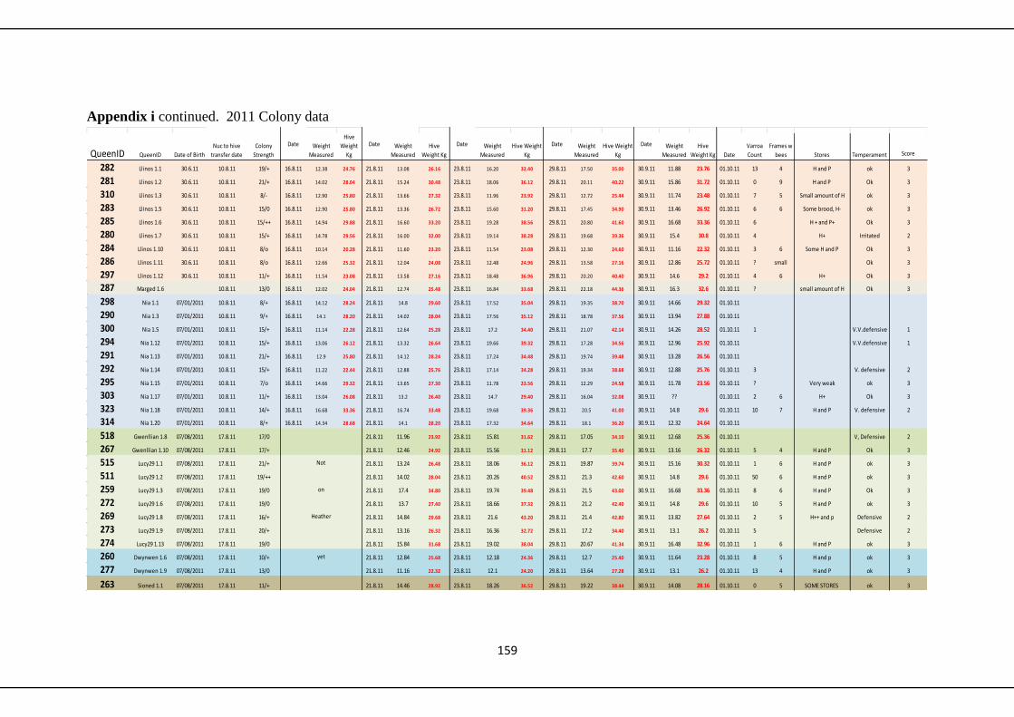
159
Appendix i continued. 2011 Colony data
Date Date Date Date Date
QueenID QueenID Score
282 Llinos 1.1 30.6.11 10.8.11 19/+ 16.8.11 12.38 24.76 21.8.11 13.08 26.16 23.8.11 16.20 32.40 29.8.11 17.50 35.00 30.9.11 11.88 23.76 01.10.11 13 4 H and P ok 3
281 Llinos 1.2 30.6.11 10.8.11 21/+ 16.8.11 14.02 28.04 21.8.11 15.24 30.48 23.8.11 18.06 36.12 29.8.11 20.11 40.22 30.9.11 15.86 31.72 01.10.11 0 9 H and P Ok 3
310 Llinos 1.3 30.6.11 10.8.11 8/- 16.8.11 12.90 25.80 21.8.11 13.66 27.32 23.8.11 11.96 23.92 29.8.11 12.72 25.44 30.9.11 11.74 23.48 01.10.11 7 5 Small amount of H ok 3
283 Llinos 1.5 30.6.11 10.8.11 15/0 16.8.11 12.90 25.80 21.8.11 13.36 26.72 23.8.11 15.60 31.20 29.8.11 17.45 34.90 30.9.11 13.46 26.92 01.10.11 6 6 Some brood, H- ok 3
285 Llinos 1.6 30.6.11 10.8.11 15/++ 16.8.11 14.94 29.88 21.8.11 16.60 33.20 23.8.11 19.28 38.56 29.8.11 20.80 41.60 30.9.11 16.68 33.36 01.10.11 6 H + and P+ Ok 3
280 Llinos 1.7 30.6.11 10.8.11 15/+ 16.8.11 14.78 29.56 21.8.11 16.00 32.00 23.8.11 19.14 38.28 29.8.11 19.68 39.36 30.9.11 15.4 30.8 01.10.11 4 H+ Irritated 2
284 Llinos 1.10 30.6.11 10.8.11 8/o 16.8.11 10.14 20.28 21.8.11 11.60 23.20 23.8.11 11.54 23.08 29.8.11 12.30 24.60 30.9.11 11.16 22.32 01.10.11 3 6 Some H and P Ok 3
286 Llinos 1.11 30.6.11 10.8.11 8/o 16.8.11 12.66 25.32 21.8.11 12.04 24.08 23.8.11 12.48 24.96 29.8.11 13.58 27.16 30.9.11 12.86 25.72 01.10.11 ? small Ok 3
297 Llinos 1.12 30.6.11 10.8.11 11/+ 16.8.11 11.54 23.08 21.8.11 13.58 27.16 23.8.11 18.48 36.96 29.8.11 20.20 40.40 30.9.11 14.6 29.2 01.10.11 4 6 H+ Ok 3
287 Marged 1.6 10.8.11 13/0 16.8.11 12.02 24.04 21.8.11 12.74 25.48 23.8.11 16.84 33.68 29.8.11 22.18 44.36 30.9.11 16.3 32.6 01.10.11 ? small amount of H Ok 3
298 Nia 1.1 07/01/2011 10.8.11 8/+ 16.8.11 14.12 28.24 21.8.11 14.8 29.60 23.8.11 17.52 35.04 29.8.11 19.35 38.70 30.9.11 14.66 29.32 01.10.11
290 Nia 1.3 07/01/2011 10.8.11 9/+ 16.8.11 14.1 28.20 21.8.11 14.02 28.04 23.8.11 17.56 35.12 29.8.11 18.78 37.56 30.9.11 13.94 27.88 01.10.11
300 Nia 1.5 07/01/2011 10.8.11 15/+ 16.8.11 11.14 22.28 21.8.11 12.64 25.28 23.8.11 17.2 34.40 29.8.11 21.07 42.14 30.9.11 14.26 28.52 01.10.11 1 V.V.defensive 1
294 Nia 1.12 07/01/2011 10.8.11 15/+ 16.8.11 13.06 26.12 21.8.11 13.32 26.64 23.8.11 19.66 39.32 29.8.11 17.28 34.56 30.9.11 12.96 25.92 01.10.11 V.V.defensive 1
291 Nia 1.13 07/01/2011 10.8.11 21/+ 16.8.11 12.9 25.80 21.8.11 14.12 28.24 23.8.11 17.24 34.48 29.8.11 19.74 39.48 30.9.11 13.28 26.56 01.10.11
292 Nia 1.14 07/01/2011 10.8.11 15/+ 16.8.11 11.22 22.44 21.8.11 12.88 25.76 23.8.11 17.14 34.28 29.8.11 19.34 38.68 30.9.11 12.88 25.76 01.10.11 3 V. defensive 2
295 Nia 1.15 07/01/2011 10.8.11 7/o 16.8.11 14.66 29.32 21.8.11 13.65 27.30 23.8.11 11.78 23.56 29.8.11 12.29 24.58 30.9.11 11.78 23.56 01.10.11 ? Very weak ok 3
303 Nia 1.17 07/01/2011 10.8.11 11/+ 16.8.11 13.04 26.08 21.8.11 13.2 26.40 23.8.11 14.7 29.40 29.8.11 16.04 32.08 30.9.11 ?? 01.10.11 2 6 H+ Ok 3
323 Nia 1.18 07/01/2011 10.8.11 14/+ 16.8.11 16.68 33.36 21.8.11 16.74 33.48 23.8.11 19.68 39.36 29.8.11 20.5 41.00 30.9.11 14.8 29.6 01.10.11 10 7 H and P V. defensive 2
314 Nia 1.20 07/01/2011 10.8.11 8/+ 16.8.11 14.34 28.68 21.8.11 14.1 28.20 23.8.11 17.32 34.64 29.8.11 18.1 36.20 30.9.11 12.32 24.64 01.10.11
518 Gwenllian 1.8 07/08/2011 17.8.11 17/0 21.8.11 11.96 23.92 23.8.11 15.81 31.62 29.8.11 17.05 34.10 30.9.11 12.68 25.36 01.10.11 V, Defensive 2
267 Gwenllian 1.10 07/08/2011 17.8.11 17/+ 21.8.11 12.46 24.92 23.8.11 15.56 31.12 29.8.11 17.7 35.40 30.9.11 13.16 26.32 01.10.11 5 4 H and P Ok 3
515 Lucy29 1.1 07/08/2011 17.8.11 21/+ Not 21.8.11 13.24 26.48 23.8.11 18.06 36.12 29.8.11 19.87 39.74 30.9.11 15.16 30.32 01.10.11 1 6 H and P ok 3
511 Lucy29 1.2 07/08/2011 17.8.11 19/++ 21.8.11 14.02 28.04 23.8.11 20.26 40.52 29.8.11 21.3 42.60 30.9.11 14.8 29.6 01.10.11 50 6 H and P ok 3
259 Lucy29 1.3 07/08/2011 17.8.11 19/0 on 21.8.11 17.4 34.80 23.8.11 19.74 39.48 29.8.11 21.5 43.00 30.9.11 16.68 33.36 01.10.11 8 6 H and P Ok 3
272 Lucy29 1.6 07/08/2011 17.8.11 19/0 21.8.11 13.7 27.40 23.8.11 18.66 37.32 29.8.11 21.2 42.40 30.9.11 14.8 29.6 01.10.11 10 5 H and P ok 3
269 Lucy29 1.8 07/08/2011 17.8.11 16/+ Heather 21.8.11 14.84 29.68 23.8.11 21.6 43.20 29.8.11 21.4 42.80 30.9.11 13.82 27.64 01.10.11 2 5 H++ and p Defensive 2
273 Lucy29 1.9 07/08/2011 17.8.11 20/+ 21.8.11 13.16 26.32 23.8.11 16.36 32.72 29.8.11 17.2 34.40 30.9.11 13.1 26.2 01.10.11 5 Defensive 2
274 Lucy29 1.13 07/08/2011 17.8.11 19/0 21.8.11 15.84 31.68 23.8.11 19.02 38.04 29.8.11 20.67 41.34 30.9.11 16.48 32.96 01.10.11 1 6 H and P ok 3
260 Dwynwen 1.6 07/08/2011 17.8.11 10/+ yet 21.8.11 12.84 25.68 23.8.11 12.18 24.36 29.8.11 12.7 25.40 30.9.11 11.64 23.28 01.10.11 8 5 H and p ok 3
277 Dwynwen 1.9 07/08/2011 17.8.11 13/0 21.8.11 11.16 22.32 23.8.11 12.1 24.20 29.8.11 13.64 27.28 30.9.11 13.1 26.2 01.10.11 13 4 H and P ok 3
263 Sioned 1.1 07/08/2011 17.8.11 11/+ 21.8.11 14.46 28.92 23.8.11 18.26 36.52 29.8.11 19.22 38.44 30.9.11 14.08 28.16 01.10.11 0 5 SOME STORES ok 3
Weight
Measured
Hive Weight
Kg
Weight
Measured
Hive Weight
Kg
Hive
Weight Kg
Nuc to hive
transfer dateDate of Birth
Colony
Strength
Weight
Measured
Hive
Weight
Kg
Weight
Measured Temperament
Weight
Measured
Hive
Weight Kg Date
Varroa
Count
Frames w
bees Stores
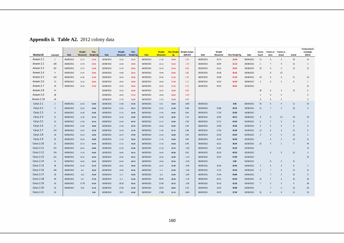
160
Appendix ii. Table A2. 2012 colony data
MotherID ColonyID Date
Weight
Measured
Hive
Weight Kg Date
Weight
Measured
Hive
Weight Kg Date
Weight
Measured
Hive Weight
Kg
Weight change
26/8-6/9 Date
Weight
Measured Hive Weight Kg Date
Varroa
Count
Frames w
bees
Frames w
brood brood
Temperament
LLandegla
4/9/12
Anwen 2.1 1 08/08/2012 13.72 27.44 26/08/2012 16.28 32.56 06/09/2012 17.30 34.60 2.04 08/09/2012 16.74 33.48 08/09/2012 11 6 3 10 15
Anwen 2.2 369 08/08/2012 14.78 29.56 26/08/2012 16.90 33.80 06/09/2012 16.12 32.24 -1.56 08/09/2012 16.09 32.18 28/08/2012 2 7 4 15 2
Anwen 2.3 287 08/08/2012 12.74 25.48 26/08/2012 15.30 30.60 06/09/2012 18.78 37.56 6.96 08/09/2012 16.52 33.04 28/08/2012 19 6 3 13 15
Anwen 2.4 9 08/08/2012 17.02 34.04 26/08/2012 19.08 38.16 06/09/2012 19.98 39.96 1.80 08/09/2012 19.28 38.56 28/08/2012 8 3.5
Anwen 2.5 419 08/08/2012 16.48 32.96 26/08/2012 18.04 36.08 06/09/2012 20.68 41.36 5.28 08/09/2012 20.98 41.96 28/08/2012 10 6 4 11 16
Anwen 2.6 13 08/08/2012 15.30 30.60 26/08/2012 18.04 36.08 06/09/2012 18.60 37.20 1.12 08/09/2012 18.24 36.48 28/08/2012 5 6 2 9 1
Anwen 2.7 26 08/08/2012 18.50 37.00 26/08/2012 19.90 39.80 06/09/2012 20.76 41.52 1.72 08/09/2012 20.42 40.84 02/09/2012 22
Anwen 2.8 47 26/08/2012 16.50 33.00 06/09/2012 16.50 33.00 0.00 30 6 3 13 0
Anwen 2.9 48 26/08/2012 18.60 37.20 06/09/2012 18.48 36.96 -0.24 1 6 4 0
Anwen 2.10 49 26/08/2012 17.50 35.00 06/09/2012 17.50 35.00 0.00 9 6 3 0
Carys 2.1 2 08/08/2012 22.30 44.60 26/08/2012 17.88 35.76 06/09/2012 9.52 19.04 -8.84 08/09/2012 0.00 08/09/2012 35 6 4 11 33
Carys 2.2 4 08/08/2012 22.40 44.80 26/08/2012 25.06 50.12 06/09/2012 25.50 51.00 0.88 08/09/2012 24.88 49.76 28/08/2012 12 7 4 18 0
Carys 2.3 8 08/08/2012 16.48 32.96 26/08/2012 17.14 34.28 06/09/2012 17.46 34.92 0.64 08/09/2012 17.50 35.00 28/08/2012
Carys 2.4 12 08/08/2012 12.08 24.16 26/08/2012 16.40 32.80 06/09/2012 19.98 39.96 7.16 08/09/2012 19.06 38.12 28/08/2012 8 6 2.5 10 19
Carys 2.5 14 08/08/2012 17.08 34.16 26/08/2012 20.38 40.76 06/09/2012 21.53 43.06 2.30 08/09/2012 21.72 43.44 02/09/2012 0 7 4 15 1
Carys 2.6 17 08/08/2012 14.40 28.80 26/08/2012 17.88 35.76 06/09/2012 19.60 39.20 3.44 08/09/2012 19.68 39.36 02/09/2012 5 6 4 9 0
Carys 2.7 376 08/08/2012 16.64 33.28 26/08/2012 16.38 32.76 06/09/2012 17.86 35.72 2.96 08/09/2012 17.50 35.00 02/09/2012 12 6 4 12 0
Carys 2.8 18 08/08/2012 16.50 33.00 26/08/2012 18.70 37.40 06/09/2012 21.40 42.80 5.40 08/09/2012 20.18 40.36 02/09/2012 3 6 3 12 2
Carys 2.9 20 08/08/2012 20.40 40.80 26/08/2012 15.28 30.56 06/09/2012 17.30 34.60 4.04 08/09/2012 18.18 36.36 02/09/2012 4 2 10 21
Carys 2.10 21 08/08/2012 16.72 33.44 26/08/2012 17.14 34.28 06/09/2012 17.34 34.68 0.40 08/09/2012 18.22 36.44 02/09/2012 25 5 2 7 44
Carys 2.11 372 08/08/2012 20.44 40.88 26/08/2012 21.90 43.80 06/09/2012 21.38 42.76 -1.04 08/09/2012 21.65 43.30 02/09/2012 13
Carys 2.12 378 08/08/2012 17.30 34.60 26/08/2012 18.08 36.16 06/09/2012 20.04 40.08 3.92 08/09/2012 20.10 40.20 02/09/2012 6 3 13 3
Carys 2.13 421 08/08/2012 18.22 36.44 26/08/2012 19.06 38.12 06/09/2012 18.49 36.98 -1.14 08/09/2012 18.54 37.08 02/09/2012 25
Carys 2.14 31 08/08/2012 16.66 33.32 26/08/2012 20.38 40.76 06/09/2012 18.28 36.56 -4.20 08/09/2012 0.00 03/09/2012 8 5 15
Carys 2.15 38 08/08/2012 16.38 32.76 26/08/2012 18.02 36.04 06/09/2012 16.54 33.08 -2.96 08/09/2012 16.46 32.92 03/09/2012 3 6 4 8 2
Carys 2.16 336 08/08/2012 18.1 36.20 26/08/2012 18.28 36.56 06/09/2012 17.5 35.00 -1.56 08/09/2012 17.22 34.44 03/09/2012 4 7 4 13 12
Carys 2.17 39 08/08/2012 16.8 33.60 26/08/2012 17.5 35.00 06/09/2012 16.5 33.00 -2.00 08/09/2012 15.44 30.88 03/09/2012 7 4 10 6
Carys 2.18 40 08/08/2012 18.7 37.40 26/08/2012 21.3 42.60 06/09/2012 20.45 40.90 -1.70 08/09/2012 20.15 40.30 03/09/2012 12 7 4 10 28
Carys 2.19 42 08/08/2012 17.78 35.56 26/08/2012 18.16 36.32 06/09/2012 17.66 35.32 -1.00 08/09/2012 16.10 32.20 03/09/2012 7 5 3 9 38
Carys 2.20 43 08/08/2012 15.6 31.20 26/08/2012 17.65 35.30 06/09/2012 19.42 38.84 3.54 08/09/2012 19.54 39.08 03/09/2012 7 4 10 40
Carys 2.21 50 0.00 26/08/2012 22.3 44.60 06/09/2012 17.88 35.76 -8.84 08/09/2012 18.70 37.40 03/09/2012 35 6 4 11 33

161
Appendix ii continued. 2012 colony data
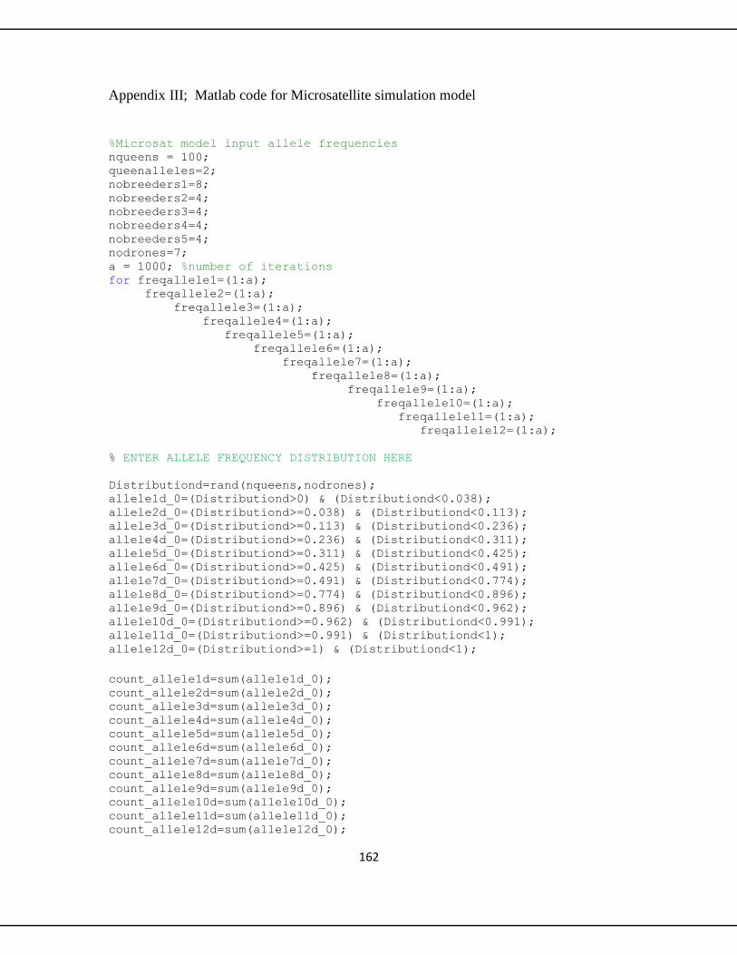
162
Appendix III; Matlab code for Microsatellite simulation model
%Microsat model input allele frequencies nqueens = 100; queenalleles=2; nobreeders1=8; nobreeders2=4; nobreeders3=4; nobreeders4=4; nobreeders5=4; nodrones=7; a = 1000; %number of iterations for freqallele1=(1:a); freqallele2=(1:a); freqallele3=(1:a); freqallele4=(1:a); freqallele5=(1:a); freqallele6=(1:a); freqallele7=(1:a); freqallele8=(1:a); freqallele9=(1:a); freqallele10=(1:a); freqallele11=(1:a); freqallele12=(1:a);
% ENTER ALLELE FREQUENCY DISTRIBUTION HERE
Distributiond=rand(nqueens,nodrones); allele1d_0=(Distributiond>0) & (Distributiond<0.038); allele2d_0=(Distributiond>=0.038) & (Distributiond<0.113); allele3d_0=(Distributiond>=0.113) & (Distributiond<0.236); allele4d_0=(Distributiond>=0.236) & (Distributiond<0.311); allele5d_0=(Distributiond>=0.311) & (Distributiond<0.425); allele6d_0=(Distributiond>=0.425) & (Distributiond<0.491); allele7d_0=(Distributiond>=0.491) & (Distributiond<0.774); allele8d_0=(Distributiond>=0.774) & (Distributiond<0.896); allele9d_0=(Distributiond>=0.896) & (Distributiond<0.962); allele10d_0=(Distributiond>=0.962) & (Distributiond<0.991); allele11d_0=(Distributiond>=0.991) & (Distributiond<1); allele12d_0=(Distributiond>=1) & (Distributiond<1);
count_allele1d=sum(allele1d_0); count_allele2d=sum(allele2d_0); count_allele3d=sum(allele3d_0); count_allele4d=sum(allele4d_0); count_allele5d=sum(allele5d_0); count_allele6d=sum(allele6d_0); count_allele7d=sum(allele7d_0); count_allele8d=sum(allele8d_0); count_allele9d=sum(allele9d_0); count_allele10d=sum(allele10d_0); count_allele11d=sum(allele11d_0); count_allele12d=sum(allele12d_0);

163
freqallele1d_0=sum(count_allele1d)/(nqueens*nodrones); freqallele2d_0=sum(count_allele2d)/(nqueens*nodrones); freqallele3d_0=sum(count_allele3d)/(nqueens*nodrones); freqallele4d_0=sum(count_allele4d)/(nqueens*nodrones); freqallele5d_0=sum(count_allele5d)/(nqueens*nodrones); freqallele6d_0=sum(count_allele6d)/(nqueens*nodrones); freqallele7d_0=sum(count_allele7d)/(nqueens*nodrones); freqallele8d_0=sum(count_allele8d)/(nqueens*nodrones); freqallele9d_0=sum(count_allele9d)/(nqueens*nodrones); freqallele10d_0=sum(count_allele10d)/(nqueens*nodrones); freqallele11d_0=sum(count_allele11d)/(nqueens*nodrones); freqallele12d_0=sum(count_allele12d)/(nqueens*nodrones);
%Describe baseline queen allele frequency dist
Distribution=rand(nqueens,queenalleles);
allele1q_0=(Distribution>0) & (Distribution<0.038); allele2q_0=(Distribution>=0.038) & (Distribution<0.113); allele3q_0=(Distribution>=0.113) & (Distribution<0.236); allele4q_0=(Distribution>=0.236) & (Distribution<0.311); allele5q_0=(Distribution>=0.311) & (Distribution<0.425); allele6q_0=(Distribution>=0.425) & (Distribution<0.491); allele7q_0=(Distribution>=0.491) & (Distribution<0.774); allele8q_0=(Distribution>=0.774) & (Distribution<0.896); allele9q_0=(Distribution>=0.896) & (Distribution<0.962); allele10q_0=(Distribution>=0.962) & (Distribution<0.991); allele11q_0=(Distribution>=0.991) & (Distribution<1); allele12q_0=(Distribution>=1) & (Distribution<1);
count_allele1q_0=sum(allele1q_0); count_allele2q_0=sum(allele2q_0); count_allele3q_0=sum(allele3q_0); count_allele4q_0=sum(allele4q_0); count_allele5q_0=sum(allele5q_0); count_allele6q_0=sum(allele6q_0); count_allele7q_0=sum(allele7q_0); count_allele8q_0=sum(allele8q_0); count_allele9q_0=sum(allele9q_0); count_allele10q_0=sum(allele10q_0); count_allele11q_0=sum(allele11q_0); count_allele12q_0=sum(allele12q_0);
freqallele1q_0=sum(count_allele1q_0)/(nqueens*queenalleles); freqallele2q_0=sum(count_allele2q_0)/(nqueens*queenalleles); freqallele3q_0=sum(count_allele3q_0)/(nqueens*queenalleles); freqallele4q_0=sum(count_allele4q_0)/(nqueens*queenalleles); freqallele5q_0=sum(count_allele5q_0)/(nqueens*queenalleles); freqallele6q_0=sum(count_allele6q_0)/(nqueens*queenalleles); freqallele7q_0=sum(count_allele7q_0)/(nqueens*queenalleles); freqallele8q_0=sum(count_allele8q_0)/(nqueens*queenalleles); freqallele9q_0=sum(count_allele9q_0)/(nqueens*queenalleles);

164
freqallele10q_0=sum(count_allele10q_0)/(nqueens*queenalleles); freqallele11q_0=sum(count_allele11q_0)/(nqueens*queenalleles); freqallele12q_0=sum(count_allele12q_0)/(nqueens*queenalleles);
%generate overall simulated population level gene distribution by adding %the weighted values of drone and queen derived alleles
freqallele1_0=((2*freqallele1d_0+freqallele1q_0)/3) freqallele2_0=((2*freqallele2d_0+freqallele2q_0)/3) freqallele3_0=((2*freqallele3d_0+freqallele3q_0)/3) freqallele4_0=((2*freqallele4d_0+freqallele4q_0)/3) freqallele5_0=((2*freqallele5d_0+freqallele5q_0)/3) freqallele6_0=((2*freqallele6d_0+freqallele6q_0)/3) freqallele7_0=((2*freqallele7d_0+freqallele7q_0)/3) freqallele8_0=((2*freqallele8d_0+freqallele8q_0)/3) freqallele9_0=((2*freqallele9d_0+freqallele9q_0)/3) freqallele10_0=((2*freqallele10d_0+freqallele10q_0)/3) freqallele11_0=((2*freqallele11d_0+freqallele11q_0)/3) freqallele12_0=((2*freqallele12d_0+freqallele12q_0)/3)
mat1_G0(freqallele1)=freqallele1_0 mat2_G0(freqallele1)=freqallele2_0 mat3_G0(freqallele1)=freqallele3_0 mat4_G0(freqallele1)=freqallele4_0 mat5_G0(freqallele1)=freqallele5_0 mat6_G0(freqallele1)=freqallele6_0 mat7_G0(freqallele1)=freqallele7_0 mat8_G0(freqallele1)=freqallele8_0 mat9_G0(freqallele1)=freqallele9_0 mat10_G0(freqallele1)=freqallele10_0 mat11_G0(freqallele1)=freqallele11_0 mat12_G0(freqallele1)=freqallele12_0
Breeders1=datasample(Distribution,nobreeders1);
allele1q_1=(Breeders1>0) & (Breeders1<freqallele1_0); allele2q_1=(Breeders1>=freqallele1_0) &
(Breeders1<(freqallele1_0+freqallele2_0)); allele3q_1=(Breeders1>=(freqallele1_0+freqallele2_0)) &
(Breeders1<(freqallele1_0+freqallele2_0+freqallele3_0)); allele4q_1=(Breeders1>=(freqallele1_0+freqallele2_0+freqallele3_0)) &
(Breeders1<(freqallele1_0+freqallele2_0+freqallele3_0+freqallele4_0)); allele5q_1=(Breeders1>=(freqallele1_0+freqallele2_0+freqallele3_0+freqalle
le4_0)) &
(Breeders1<(freqallele1_0+freqallele2_0+freqallele3_0+freqallele4_0+freqal
lele5_0)); allele6q_1=(Breeders1>=(freqallele1_0+freqallele2_0+freqallele3_0+freqalle
le4_0+freqallele5_0)) &
(Breeders1<(freqallele1_0+freqallele2_0+freqallele3_0+freqallele4_0+freqal
lele5_0+freqallele6_0)); allele7q_1=(Breeders1>=(freqallele1_0+freqallele2_0+freqallele3_0+freqalle
le4_0+freqallele5_0+freqallele6_0)) &
165
(Breeders1<(freqallele1_0+freqallele2_0+freqallele3_0+freqallele4_0+freqal
lele5_0+freqallele6_0+freqallele7_0)); allele8q_1=(Breeders1>=(freqallele1_0+freqallele2_0+freqallele3_0+freqalle
le4_0+freqallele5_0+freqallele6_0+freqallele7_0)) &
(Breeders1<(freqallele1_0+freqallele2_0+freqallele3_0+freqallele4_0+freqal
lele5_0+freqallele6_0+freqallele7_0+freqallele8_0)); allele9q_1=(Breeders1>=(freqallele1_0+freqallele2_0+freqallele3_0+freqalle
le4_0+freqallele5_0+freqallele6_0+freqallele7_0+freqallele8_0)) &
(Breeders1<(freqallele1_0+freqallele2_0+freqallele3_0+freqallele4_0+freqal
lele5_0+freqallele6_0+freqallele7_0+freqallele8_0+freqallele9_0)); allele10q_1=(Breeders1>=(freqallele1_0+freqallele2_0+freqallele3_0+freqall
ele4_0+freqallele5_0+freqallele6_0+freqallele7_0+freqallele8_0+freqallele9
_0)) &
(Breeders1<(freqallele1_0+freqallele2_0+freqallele3_0+freqallele4_0+freqal
lele5_0+freqallele6_0+freqallele7_0+freqallele8_0+freqallele9_0+freqallele
10_0)); allele11q_1=(Breeders1>=(freqallele1_0+freqallele2_0+freqallele3_0+freqall
ele4_0+freqallele5_0+freqallele6_0+freqallele7_0+freqallele8_0+freqallele9
_0+freqallele10_0)) &
(Breeders1<(freqallele1_0+freqallele2_0+freqallele3_0+freqallele4_0+freqal
lele5_0+freqallele6_0+freqallele7_0+freqallele8_0+freqallele9_0+freqallele
10_0+freqallele11_0)); allele12q_1=(Breeders1>=(freqallele1_0+freqallele2_0+freqallele3_0+freqall
ele4_0+freqallele5_0+freqallele6_0+freqallele7_0+freqallele8_0+freqallele9
_0+freqallele10_0+freqallele11_0)) & (Breeders1<1.0);
count_allele1q_1=sum(allele1q_1); count_allele2q_1=sum(allele2q_1); count_allele3q_1=sum(allele3q_1); count_allele4q_1=sum(allele4q_1); count_allele5q_1=sum(allele5q_1); count_allele6q_1=sum(allele6q_1); count_allele7q_1=sum(allele7q_1); count_allele8q_1=sum(allele8q_1); count_allele9q_1=sum(allele9q_1); count_allele10q_1=sum(allele10q_1); count_allele11q_1=sum(allele11q_1); count_allele12q_1=sum(allele12q_1);
freqallele1q_1=sum(count_allele1q_1)/(nobreeders1*queenalleles); freqallele2q_1=sum(count_allele2q_1)/(nobreeders1*queenalleles); freqallele3q_1=sum(count_allele3q_1)/(nobreeders1*queenalleles); freqallele4q_1=sum(count_allele4q_1)/(nobreeders1*queenalleles); freqallele5q_1=sum(count_allele5q_1)/(nobreeders1*queenalleles); freqallele6q_1=sum(count_allele6q_1)/(nobreeders1*queenalleles); freqallele7q_1=sum(count_allele7q_1)/(nobreeders1*queenalleles); freqallele8q_1=sum(count_allele8q_1)/(nobreeders1*queenalleles); freqallele9q_1=sum(count_allele9q_1)/(nobreeders1*queenalleles); freqallele10q_1=sum(count_allele10q_1)/(nobreeders1*queenalleles); freqallele11q_1=sum(count_allele11q_1)/(nobreeders1*queenalleles); freqallele12q_1=sum(count_allele12q_1)/(nobreeders1*queenalleles);
Ballelefreq1_G1=(2*freqallele1q_1+freqallele1d_0)/3

166
Ballelefreq2_G1=(2*freqallele2q_1+freqallele2d_0)/3 Ballelefreq3_G1=(2*freqallele3q_1+freqallele3d_0)/3 Ballelefreq4_G1=(2*freqallele4q_1+freqallele4d_0)/3 Ballelefreq5_G1=(2*freqallele5q_1+freqallele5d_0)/3 Ballelefreq6_G1=(2*freqallele6q_1+freqallele6d_0)/3 Ballelefreq7_G1=(2*freqallele7q_1+freqallele7d_0)/3 Ballelefreq8_G1=(2*freqallele8q_1+freqallele8d_0)/3 Ballelefreq9_G1=(2*freqallele9q_1+freqallele9d_0)/3 Ballelefreq10_G1=(2*freqallele10q_1+freqallele10d_0)/3 Ballelefreq11_G1=(2*freqallele11q_1+freqallele11d_0)/3 Ballelefreq12_G1=(2*freqallele12q_1+freqallele12d_0)/3
%GENERATE 100 QUEENS WITH ABOVE DISTRIBUTION DistGen1Q=rand(nqueens,queenalleles) ;
allele1q_1=(DistGen1Q>0) & (DistGen1Q<Ballelefreq1_G1); allele2q_1=(DistGen1Q>=Ballelefreq1_G1) &
(DistGen1Q<(Ballelefreq1_G1+Ballelefreq2_G1)); allele3q_1=(DistGen1Q>=(Ballelefreq1_G1+Ballelefreq2_G1)) &
(DistGen1Q<(Ballelefreq1_G1+Ballelefreq2_G1+Ballelefreq3_G1)); allele4q_1=(DistGen1Q>=(Ballelefreq1_G1+Ballelefreq2_G1+Ballelefreq3_G1))
&
(DistGen1Q<(Ballelefreq1_G1+Ballelefreq2_G1+Ballelefreq3_G1+Ballelefreq4_G
1)); allele5q_1=(DistGen1Q>=(Ballelefreq1_G1+Ballelefreq2_G1+Ballelefreq3_G1+Ba
llelefreq4_G1)) &
(DistGen1Q<(Ballelefreq1_G1+Ballelefreq2_G1+Ballelefreq3_G1+Ballelefreq4_G
1+Ballelefreq5_G1)); allele6q_1=(DistGen1Q>=(Ballelefreq1_G1+Ballelefreq2_G1+Ballelefreq3_G1+Ba
llelefreq4_G1+Ballelefreq5_G1)) &
(DistGen1Q<(Ballelefreq1_G1+Ballelefreq2_G1+Ballelefreq3_G1+Ballelefreq4_G
1+Ballelefreq5_G1+Ballelefreq6_G1)); allele7q_1=(DistGen1Q>=(Ballelefreq1_G1+Ballelefreq2_G1+Ballelefreq3_G1+Ba
llelefreq4_G1+Ballelefreq5_G1+Ballelefreq6_G1)) &
(DistGen1Q<(Ballelefreq1_G1+Ballelefreq2_G1+Ballelefreq3_G1+Ballelefreq4_G
1+Ballelefreq5_G1+Ballelefreq6_G1+Ballelefreq7_G1)); allele8q_1=(DistGen1Q>=(Ballelefreq1_G1+Ballelefreq2_G1+Ballelefreq3_G1+Ba
llelefreq4_G1+Ballelefreq5_G1+Ballelefreq6_G1+Ballelefreq7_G1)) &
(DistGen1Q<(Ballelefreq1_G1+Ballelefreq2_G1+Ballelefreq3_G1+Ballelefreq4_G
1+Ballelefreq5_G1+Ballelefreq6_G1+Ballelefreq7_G1+Ballelefreq8_G1)); allele9q_1=(DistGen1Q>=(Ballelefreq1_G1+Ballelefreq2_G1+Ballelefreq3_G1+Ba
llelefreq4_G1+Ballelefreq5_G1+Ballelefreq6_G1+Ballelefreq7_G1+Ballelefreq8
_G1)) &
(DistGen1Q<(Ballelefreq1_G1+Ballelefreq2_G1+Ballelefreq3_G1+Ballelefreq4_G
1+Ballelefreq5_G1+Ballelefreq6_G1+Ballelefreq7_G1+Ballelefreq8_G1+Ballelef
req9_G1)); allele10q_1=(DistGen1Q>=(Ballelefreq1_G1+Ballelefreq2_G1+Ballelefreq3_G1+B
allelefreq4_G1+Ballelefreq5_G1+Ballelefreq6_G1+Ballelefreq7_G1+Ballelefreq
8_G1+Ballelefreq9_G1)) &
(DistGen1Q<(Ballelefreq1_G1+Ballelefreq2_G1+Ballelefreq3_G1+Ballelefreq4_G
1+Ballelefreq5_G1+Ballelefreq6_G1+Ballelefreq7_G1+Ballelefreq8_G1+Ballelef
req9_G1+Ballelefreq10_G1));
167
allele11q_1=(DistGen1Q>=(Ballelefreq1_G1+Ballelefreq2_G1+Ballelefreq3_G1+B
allelefreq4_G1+Ballelefreq5_G1+Ballelefreq6_G1+Ballelefreq7_G1+Ballelefreq
8_G1+Ballelefreq9_G1+Ballelefreq10_G1)) &
(DistGen1Q<(Ballelefreq1_G1+Ballelefreq2_G1+Ballelefreq3_G1+Ballelefreq4_G
1+Ballelefreq5_G1+Ballelefreq6_G1+Ballelefreq7_G1+Ballelefreq8_G1+Ballelef
req9_G1+Ballelefreq10_G1+Ballelefreq11_G1)); allele12q_1=(DistGen1Q>=(Ballelefreq1_G1+Ballelefreq2_G1+Ballelefreq3_G1+B
allelefreq4_G1+Ballelefreq5_G1+Ballelefreq6_G1+Ballelefreq7_G1+Ballelefreq
8_G1+Ballelefreq9_G1+Ballelefreq10_G1+Ballelefreq11_G1)) & (DistGen1Q<1);
count_allele1q_1=sum(allele1q_1); count_allele2q_1=sum(allele2q_1); count_allele3q_1=sum(allele3q_1); count_allele4q_1=sum(allele4q_1); count_allele5q_1=sum(allele5q_1); count_allele6q_1=sum(allele6q_1); count_allele7q_1=sum(allele7q_1); count_allele8q_1=sum(allele8q_1); count_allele9q_1=sum(allele9q_1); count_allele10q_1=sum(allele10q_1); count_allele11q_1=sum(allele11q_1); count_allele12q_1=sum(allele12q_1);
freqallele1q_1=sum(count_allele1q_1)/(nqueens*queenalleles) freqallele2q_1=sum(count_allele2q_1)/(nqueens*queenalleles) freqallele3q_1=sum(count_allele3q_1)/(nqueens*queenalleles) freqallele4q_1=sum(count_allele4q_1)/(nqueens*queenalleles) freqallele5q_1=sum(count_allele5q_1)/(nqueens*queenalleles) freqallele6q_1=sum(count_allele6q_1)/(nqueens*queenalleles) freqallele7q_1=sum(count_allele7q_1)/(nqueens*queenalleles) freqallele8q_1=sum(count_allele8q_1)/(nqueens*queenalleles) freqallele9q_1=sum(count_allele9q_1)/(nqueens*queenalleles) freqallele10q_1=sum(count_allele10q_1)/(nqueens*queenalleles) freqallele11q_1=sum(count_allele11q_1)/(nqueens*queenalleles) freqallele12q_1=sum(count_allele12q_1)/(nqueens*queenalleles)
freqallele1_1=((2*freqallele1q_1+freqallele1d_0)/3) freqallele2_1=((2*freqallele2q_1+freqallele2d_0)/3) freqallele3_1=((2*freqallele3q_1+freqallele3d_0)/3) freqallele4_1=((2*freqallele4q_1+freqallele4d_0)/3) freqallele5_1=((2*freqallele5q_1+freqallele5d_0)/3) freqallele6_1=((2*freqallele6q_1+freqallele6d_0)/3) freqallele7_1=((2*freqallele7q_1+freqallele7d_0)/3) freqallele8_1=((2*freqallele8q_1+freqallele8d_0)/3) freqallele9_1=((2*freqallele9q_1+freqallele9d_0)/3) freqallele10_1=((2*freqallele10q_1+freqallele10d_0)/3) freqallele11_1=((2*freqallele11q_1+freqallele11d_0)/3) freqallele12_1=((2*freqallele12q_1+freqallele12d_0)/3)
mat1_G1(freqallele1)=freqallele1_1 mat2_G1(freqallele1)=freqallele2_1 mat3_G1(freqallele1)=freqallele3_1 mat4_G1(freqallele1)=freqallele4_1 mat5_G1(freqallele1)=freqallele5_1

168
mat6_G1(freqallele1)=freqallele6_1 mat7_G1(freqallele1)=freqallele7_1 mat8_G1(freqallele1)=freqallele8_1 mat9_G1(freqallele1)=freqallele9_1 mat10_G1(freqallele1)=freqallele10_1 mat11_G1(freqallele1)=freqallele11_1 mat12_G1(freqallele1)=freqallele12_1
Breeders2=datasample(Distribution,nobreeders2);
allele1q_2=(Breeders2>0) & (Breeders2<freqallele1_1); allele2q_2=(Breeders2>=freqallele1_1) &
(Breeders2<(freqallele1_1+freqallele2_1)); allele3q_2=(Breeders2>=(freqallele1_1+freqallele2_1)) &
(Breeders2<(freqallele1_1+freqallele2_1+freqallele3_1)); allele4q_2=(Breeders2>=(freqallele1_1+freqallele2_1+freqallele3_1)) &
(Breeders2<(freqallele1_1+freqallele2_1+freqallele3_1+freqallele4_1)); allele5q_2=(Breeders2>=(freqallele1_1+freqallele2_1+freqallele3_1+freqalle
le4_1)) &
(Breeders2<(freqallele1_1+freqallele2_1+freqallele3_1+freqallele4_1+freqal
lele5_1)); allele6q_2=(Breeders2>=(freqallele1_1+freqallele2_1+freqallele3_1+freqalle
le4_1+freqallele5_1)) &
(Breeders2<(freqallele1_1+freqallele2_1+freqallele3_1+freqallele4_1+freqal
lele5_1+freqallele6_1)); allele7q_2=(Breeders2>=(freqallele1_1+freqallele2_1+freqallele3_1+freqalle
le4_1+freqallele5_1+freqallele6_1)) &
(Breeders2<(freqallele1_1+freqallele2_1+freqallele3_1+freqallele4_1+freqal
lele5_1+freqallele6_1+freqallele7_1)); allele8q_2=(Breeders2>=(freqallele1_1+freqallele2_1+freqallele3_1+freqalle
le4_1+freqallele5_1+freqallele6_1+freqallele7_1)) &
(Breeders2<(freqallele1_1+freqallele2_1+freqallele3_1+freqallele4_1+freqal
lele5_1+freqallele6_1+freqallele7_1+freqallele8_1)); allele9q_2=(Breeders2>=(freqallele1_1+freqallele2_1+freqallele3_1+freqalle
le4_1+freqallele5_1+freqallele6_1+freqallele7_1+freqallele8_1)) &
(Breeders2<(freqallele1_1+freqallele2_1+freqallele3_1+freqallele4_1+freqal
lele5_1+freqallele6_1+freqallele7_1+freqallele8_1+freqallele9_1)); allele10q_2=(Breeders2>=(freqallele1_1+freqallele2_1+freqallele3_1+freqall
ele4_1+freqallele5_1+freqallele6_1+freqallele7_1+freqallele8_1+freqallele9
_1)) &
(Breeders2<(freqallele1_1+freqallele2_1+freqallele3_1+freqallele4_1+freqal
lele5_1+freqallele6_1+freqallele7_1+freqallele8_1+freqallele9_1+freqallele
10_1)); allele11q_2=(Breeders2>=(freqallele1_1+freqallele2_1+freqallele3_1+freqall
ele4_1+freqallele5_1+freqallele6_1+freqallele7_1+freqallele8_1+freqallele9
_1+freqallele10_1)) &
(Breeders2<(freqallele1_1+freqallele2_1+freqallele3_1+freqallele4_1+freqal
lele5_1+freqallele6_1+freqallele7_1+freqallele8_1+freqallele9_1+freqallele
10_1+freqallele11_1)); allele12q_2=(Breeders2>=(freqallele1_1+freqallele2_1+freqallele3_1+freqall
ele4_1+freqallele5_1+freqallele6_1+freqallele7_1+freqallele8_1+freqallele9
_1+freqallele10_1+freqallele11_1)) & (Breeders2<1.0);

169
count_allele1q_2=sum(allele1q_2); count_allele2q_2=sum(allele2q_2); count_allele3q_2=sum(allele3q_2); count_allele4q_2=sum(allele4q_2); count_allele5q_2=sum(allele5q_2); count_allele6q_2=sum(allele6q_2); count_allele7q_2=sum(allele7q_2); count_allele8q_2=sum(allele8q_2); count_allele9q_2=sum(allele9q_2); count_allele10q_2=sum(allele10q_2); count_allele11q_2=sum(allele11q_2); count_allele12q_2=sum(allele12q_2);
freqallele1q_2=sum(count_allele1q_2)/(nobreeders2*queenalleles); freqallele2q_2=sum(count_allele2q_2)/(nobreeders2*queenalleles); freqallele3q_2=sum(count_allele3q_2)/(nobreeders2*queenalleles); freqallele4q_2=sum(count_allele4q_2)/(nobreeders2*queenalleles); freqallele5q_2=sum(count_allele5q_2)/(nobreeders2*queenalleles); freqallele6q_2=sum(count_allele6q_2)/(nobreeders2*queenalleles); freqallele7q_2=sum(count_allele7q_2)/(nobreeders2*queenalleles); freqallele8q_2=sum(count_allele8q_2)/(nobreeders2*queenalleles); freqallele9q_2=sum(count_allele9q_2)/(nobreeders2*queenalleles); freqallele10q_2=sum(count_allele10q_2)/(nobreeders2*queenalleles); freqallele11q_2=sum(count_allele11q_2)/(nobreeders2*queenalleles); freqallele12q_2=sum(count_allele12q_2)/(nobreeders2*queenalleles);
Ballelefreq1_G2=(2*freqallele1q_2+freqallele1q_1)/3 Ballelefreq2_G2=(2*freqallele2q_2+freqallele2q_1)/3 Ballelefreq3_G2=(2*freqallele3q_2+freqallele3q_1)/3 Ballelefreq4_G2=(2*freqallele4q_2+freqallele4q_1)/3 Ballelefreq5_G2=(2*freqallele5q_2+freqallele5q_1)/3 Ballelefreq6_G2=(2*freqallele6q_2+freqallele6q_1)/3 Ballelefreq7_G2=(2*freqallele7q_2+freqallele7q_1)/3 Ballelefreq8_G2=(2*freqallele8q_2+freqallele8q_1)/3 Ballelefreq9_G2=(2*freqallele9q_2+freqallele9q_1)/3 Ballelefreq10_G2=(2*freqallele10q_2+freqallele10q_1)/3 Ballelefreq11_G2=(2*freqallele11q_2+freqallele11q_1)/3 Ballelefreq12_G2=(2*freqallele12q_2+freqallele12q_1)/3
%GENERATE 100 NEW QUEEN GENOTYPES FROM THIS FREQUENCY DISTRIBUTION
DistGen2Q=rand(nqueens,queenalleles);
allele1q_2=(DistGen2Q>0) & (DistGen2Q<Ballelefreq1_G2); allele2q_2=(DistGen2Q>=Ballelefreq1_G2) &
(DistGen2Q<(Ballelefreq1_G2+Ballelefreq2_G2)); allele3q_2=(DistGen2Q>=(Ballelefreq1_G2+Ballelefreq2_G2)) &
(DistGen2Q<(Ballelefreq1_G2+Ballelefreq2_G2+Ballelefreq3_G2)); allele4q_2=(DistGen2Q>=(Ballelefreq1_G2+Ballelefreq2_G2+Ballelefreq3_G2))
&
(DistGen2Q<(Ballelefreq1_G2+Ballelefreq2_G2+Ballelefreq3_G2+Ballelefreq4_G
2)); allele5q_2=(DistGen2Q>=(Ballelefreq1_G2+Ballelefreq2_G2+Ballelefreq3_G2+Ba
llelefreq4_G2)) &

170
(DistGen2Q<(Ballelefreq1_G2+Ballelefreq2_G2+Ballelefreq3_G2+Ballelefreq4_G
2+Ballelefreq5_G2)); allele6q_2=(DistGen2Q>=(Ballelefreq1_G2+Ballelefreq2_G2+Ballelefreq3_G2+Ba
llelefreq4_G2+Ballelefreq5_G2)) &
(DistGen2Q<(Ballelefreq1_G2+Ballelefreq2_G2+Ballelefreq3_G2+Ballelefreq4_G
2+Ballelefreq5_G2+Ballelefreq6_G2)); allele7q_2=(DistGen2Q>=(Ballelefreq1_G2+Ballelefreq2_G2+Ballelefreq3_G2+Ba
llelefreq4_G2+Ballelefreq5_G2+Ballelefreq6_G2)) &
(DistGen2Q<(Ballelefreq1_G2+Ballelefreq2_G2+Ballelefreq3_G2+Ballelefreq4_G
2+Ballelefreq5_G2+Ballelefreq6_G2+Ballelefreq7_G2)); allele8q_2=(DistGen2Q>=(Ballelefreq1_G2+Ballelefreq2_G2+Ballelefreq3_G2+Ba
llelefreq4_G2+Ballelefreq5_G2+Ballelefreq6_G2+Ballelefreq7_G2)) &
(DistGen2Q<(Ballelefreq1_G2+Ballelefreq2_G2+Ballelefreq3_G2+Ballelefreq4_G
2+Ballelefreq5_G2+Ballelefreq6_G2+Ballelefreq7_G2+Ballelefreq8_G2)); allele9q_2=(DistGen2Q>=(Ballelefreq1_G2+Ballelefreq2_G2+Ballelefreq3_G2+Ba
llelefreq4_G2+Ballelefreq5_G2+Ballelefreq6_G2+Ballelefreq7_G2+Ballelefreq8
_G2)) &
(DistGen2Q<(Ballelefreq1_G2+Ballelefreq2_G2+Ballelefreq3_G2+Ballelefreq4_G
2+Ballelefreq5_G2+Ballelefreq6_G2+Ballelefreq7_G2+Ballelefreq8_G2+Ballelef
req9_G2)); allele10q_2=(DistGen2Q>=(Ballelefreq1_G2+Ballelefreq2_G2+Ballelefreq3_G2+B
allelefreq4_G2+Ballelefreq5_G2+Ballelefreq6_G2+Ballelefreq7_G2+Ballelefreq
8_G2+Ballelefreq9_G2)) &
(DistGen2Q<(Ballelefreq1_G2+Ballelefreq2_G2+Ballelefreq3_G2+Ballelefreq4_G
2+Ballelefreq5_G2+Ballelefreq6_G2+Ballelefreq7_G2+Ballelefreq8_G2+Ballelef
req9_G2+Ballelefreq10_G2)); allele11q_2=(DistGen2Q>=(Ballelefreq1_G2+Ballelefreq2_G2+Ballelefreq3_G2+B
allelefreq4_G2+Ballelefreq5_G2+Ballelefreq6_G2+Ballelefreq7_G2+Ballelefreq
8_G2+Ballelefreq9_G2+Ballelefreq10_G2)) &
(DistGen2Q<(Ballelefreq1_G2+Ballelefreq2_G2+Ballelefreq3_G2+Ballelefreq4_G
2+Ballelefreq5_G2+Ballelefreq6_G2+Ballelefreq7_G2+Ballelefreq8_G2+Ballelef
req9_G2+Ballelefreq10_G2+Ballelefreq11_G2)); allele12q_2=(DistGen2Q>=(Ballelefreq1_G2+Ballelefreq2_G2+Ballelefreq3_G2+B
allelefreq4_G2+Ballelefreq5_G2+Ballelefreq6_G2+Ballelefreq7_G2+Ballelefreq
8_G2+Ballelefreq9_G2+Ballelefreq10_G2+Ballelefreq11_G2)) & (DistGen2Q<1);
count_allele1q_2=sum(allele1q_2); count_allele2q_2=sum(allele2q_2); count_allele3q_2=sum(allele3q_2); count_allele4q_2=sum(allele4q_2); count_allele5q_2=sum(allele5q_2); count_allele6q_2=sum(allele6q_2); count_allele7q_2=sum(allele7q_2); count_allele8q_2=sum(allele8q_2); count_allele9q_2=sum(allele9q_2); count_allele10q_2=sum(allele10q_2); count_allele11q_2=sum(allele11q_2); count_allele12q_2=sum(allele12q_2);
freqallele1q_2=sum(count_allele1q_2)/(nqueens*queenalleles); freqallele2q_2=sum(count_allele2q_2)/(nqueens*queenalleles); freqallele3q_2=sum(count_allele3q_2)/(nqueens*queenalleles); freqallele4q_2=sum(count_allele4q_2)/(nqueens*queenalleles); freqallele5q_2=sum(count_allele5q_2)/(nqueens*queenalleles); freqallele6q_2=sum(count_allele6q_2)/(nqueens*queenalleles);
171
freqallele7q_2=sum(count_allele7q_2)/(nqueens*queenalleles); freqallele8q_2=sum(count_allele8q_2)/(nqueens*queenalleles); freqallele9q_2=sum(count_allele9q_2)/(nqueens*queenalleles); freqallele10q_2=sum(count_allele10q_2)/(nqueens*queenalleles); freqallele11q_2=sum(count_allele11q_2)/(nqueens*queenalleles); freqallele12q_2=sum(count_allele12q_2)/(nqueens*queenalleles);
freqallele1_2=((2*freqallele1q_2+freqallele1q_1)/3) freqallele2_2=((2*freqallele2q_2+freqallele2q_1)/3) freqallele3_2=((2*freqallele3q_2+freqallele3q_1)/3) freqallele4_2=((2*freqallele4q_2+freqallele4q_1)/3) freqallele5_2=((2*freqallele5q_2+freqallele5q_1)/3) freqallele6_2=((2*freqallele6q_2+freqallele6q_1)/3) freqallele7_2=((2*freqallele7q_2+freqallele7q_1)/3) freqallele8_2=((2*freqallele8q_2+freqallele8q_1)/3) freqallele9_2=((2*freqallele9q_2+freqallele9q_1)/3) freqallele10_2=((2*freqallele10q_2+freqallele10q_1)/3) freqallele11_2=((2*freqallele11q_2+freqallele11q_1)/3) freqallele12_2=((2*freqallele12q_2+freqallele12q_1)/3)
mat1_G2(freqallele1)=freqallele1_2 mat2_G2(freqallele1)=freqallele2_2 mat3_G2(freqallele1)=freqallele3_2 mat4_G2(freqallele1)=freqallele4_2 mat5_G2(freqallele1)=freqallele5_2 mat6_G2(freqallele1)=freqallele6_2 mat7_G2(freqallele1)=freqallele7_2 mat8_G2(freqallele1)=freqallele8_2 mat9_G2(freqallele1)=freqallele9_2 mat10_G2(freqallele1)=freqallele10_2 mat11_G2(freqallele1)=freqallele11_2 mat12_G2(freqallele1)=freqallele12_2
Breeders3=datasample(Distribution,nobreeders3); allele1q_3=(Breeders3>0) & (Breeders3<freqallele1_2); allele2q_3=(Breeders3>=freqallele1_2) &
(Breeders3<(freqallele1_2+freqallele2_2)); allele3q_3=(Breeders3>=(freqallele1_2+freqallele2_2)) &
(Breeders3<(freqallele1_2+freqallele2_2+freqallele3_2)); allele4q_3=(Breeders3>=(freqallele1_2+freqallele2_2+freqallele3_2)) &
(Breeders3<(freqallele1_2+freqallele2_2+freqallele3_2+freqallele4_2)); allele5q_3=(Breeders3>=(freqallele1_2+freqallele2_2+freqallele3_2+freqalle
le4_2)) &
(Breeders3<(freqallele1_2+freqallele2_2+freqallele3_2+freqallele4_2+freqal
lele5_2)); allele6q_3=(Breeders3>=(freqallele1_2+freqallele2_2+freqallele3_2+freqalle
le4_2+freqallele5_2)) &
(Breeders3<(freqallele1_2+freqallele2_2+freqallele3_2+freqallele4_2+freqal
lele5_2+freqallele6_2)); allele7q_3=(Breeders3>=(freqallele1_2+freqallele2_2+freqallele3_2+freqalle
le4_2+freqallele5_2+freqallele6_2)) &
(Breeders3<(freqallele1_2+freqallele2_2+freqallele3_2+freqallele4_2+freqal
lele5_2+freqallele6_2+freqallele7_2));
172
allele8q_3=(Breeders3>=(freqallele1_2+freqallele2_2+freqallele3_2+freqalle
le4_2+freqallele5_2+freqallele6_2+freqallele7_2)) &
(Breeders3<(freqallele1_2+freqallele2_2+freqallele3_2+freqallele4_2+freqal
lele5_2+freqallele6_2+freqallele7_2+freqallele8_2)); allele9q_3=(Breeders3>=(freqallele1_2+freqallele2_2+freqallele3_2+freqalle
le4_2+freqallele5_2+freqallele6_2+freqallele7_2+freqallele8_2)) &
(Breeders3<(freqallele1_2+freqallele2_2+freqallele3_2+freqallele4_2+freqal
lele5_2+freqallele6_2+freqallele7_2+freqallele8_2+freqallele9_2)); allele10q_3=(Breeders3>=(freqallele1_2+freqallele2_2+freqallele3_2+freqall
ele4_2+freqallele5_2+freqallele6_2+freqallele7_2+freqallele8_2+freqallele9
_2)) &
(Breeders3<(freqallele1_2+freqallele2_2+freqallele3_2+freqallele4_2+freqal
lele5_2+freqallele6_2+freqallele7_2+freqallele8_2+freqallele9_2+freqallele
10_2)); allele11q_3=(Breeders3>=(freqallele1_2+freqallele2_2+freqallele3_2+freqall
ele4_2+freqallele5_2+freqallele6_2+freqallele7_2+freqallele8_2+freqallele9
_2+freqallele10_2)) &
(Breeders3<(freqallele1_2+freqallele2_2+freqallele3_2+freqallele4_2+freqal
lele5_2+freqallele6_2+freqallele7_2+freqallele8_2+freqallele9_2+freqallele
10_2+freqallele11_2)); allele12q_3=(Breeders3>=(freqallele1_2+freqallele2_2+freqallele3_2+freqall
ele4_2+freqallele5_2+freqallele6_2+freqallele7_2+freqallele8_2+freqallele9
_2+freqallele10_2+freqallele11_2)) & (Breeders3<1.0);
count_allele1q_3=sum(allele1q_3); count_allele2q_3=sum(allele2q_3); count_allele3q_3=sum(allele3q_3); count_allele4q_3=sum(allele4q_3); count_allele5q_3=sum(allele5q_3); count_allele6q_3=sum(allele6q_3); count_allele7q_3=sum(allele7q_3); count_allele8q_3=sum(allele8q_3); count_allele9q_3=sum(allele9q_3); count_allele10q_3=sum(allele10q_3); count_allele11q_3=sum(allele11q_3); count_allele12q_3=sum(allele12q_3);
freqallele1q_3=sum(count_allele1q_3)/(nobreeders3*queenalleles); freqallele2q_3=sum(count_allele2q_3)/(nobreeders3*queenalleles); freqallele3q_3=sum(count_allele3q_3)/(nobreeders3*queenalleles); freqallele4q_3=sum(count_allele4q_3)/(nobreeders3*queenalleles); freqallele5q_3=sum(count_allele5q_3)/(nobreeders3*queenalleles); freqallele6q_3=sum(count_allele6q_3)/(nobreeders3*queenalleles); freqallele7q_3=sum(count_allele7q_3)/(nobreeders3*queenalleles); freqallele8q_3=sum(count_allele8q_3)/(nobreeders3*queenalleles); freqallele9q_3=sum(count_allele9q_3)/(nobreeders3*queenalleles); freqallele10q_3=sum(count_allele10q_3)/(nobreeders3*queenalleles); freqallele11q_3=sum(count_allele11q_3)/(nobreeders3*queenalleles); freqallele12q_3=sum(count_allele12q_3)/(nobreeders3*queenalleles);
Ballelefreq1_G3=(2*freqallele1q_3+freqallele1q_2)/3 Ballelefreq2_G3=(2*freqallele2q_3+freqallele2q_2)/3 Ballelefreq3_G3=(2*freqallele3q_3+freqallele3q_2)/3
173
Ballelefreq4_G3=(2*freqallele4q_3+freqallele4q_2)/3 Ballelefreq5_G3=(2*freqallele5q_3+freqallele5q_2)/3 Ballelefreq6_G3=(2*freqallele6q_3+freqallele6q_2)/3 Ballelefreq7_G3=(2*freqallele7q_3+freqallele7q_2)/3 Ballelefreq8_G3=(2*freqallele8q_3+freqallele8q_2)/3 Ballelefreq9_G3=(2*freqallele9q_3+freqallele9q_2)/3 Ballelefreq10_G3=(2*freqallele10q_3+freqallele10q_2)/3 Ballelefreq11_G3=(2*freqallele11q_3+freqallele11q_2)/3 Ballelefreq12_G3=(2*freqallele12q_3+freqallele12q_2)/3
%GENERATE 100 QUEENS DistGen3Q=rand(nqueens,queenalleles);
allele1q_3=(DistGen3Q>0) & (DistGen3Q<Ballelefreq1_G3); allele2q_3=(DistGen3Q>=Ballelefreq1_G3) &
(DistGen3Q<(Ballelefreq1_G3+Ballelefreq2_G3)); allele3q_3=(DistGen3Q>=(Ballelefreq1_G3+Ballelefreq2_G3)) &
(DistGen3Q<(Ballelefreq1_G3+Ballelefreq2_G3+Ballelefreq3_G3)); allele4q_3=(DistGen3Q>=(Ballelefreq1_G3+Ballelefreq2_G3+Ballelefreq3_G3))
&
(DistGen3Q<(Ballelefreq1_G3+Ballelefreq2_G3+Ballelefreq3_G3+Ballelefreq4_G
3)); allele5q_3=(DistGen3Q>=(Ballelefreq1_G3+Ballelefreq2_G3+Ballelefreq3_G3+Ba
llelefreq4_G3)) &
(DistGen3Q<(Ballelefreq1_G3+Ballelefreq2_G3+Ballelefreq3_G3+Ballelefreq4_G
3+Ballelefreq5_G3)); allele6q_3=(DistGen3Q>=(Ballelefreq1_G3+Ballelefreq2_G3+Ballelefreq3_G3+Ba
llelefreq4_G3+Ballelefreq5_G3)) &
(DistGen3Q<(Ballelefreq1_G3+Ballelefreq2_G3+Ballelefreq3_G3+Ballelefreq4_G
3+Ballelefreq5_G3+Ballelefreq6_G3)); allele7q_3=(DistGen3Q>=(Ballelefreq1_G3+Ballelefreq2_G3+Ballelefreq3_G3+Ba
llelefreq4_G3+Ballelefreq5_G3+Ballelefreq6_G3)) &
(DistGen3Q<(Ballelefreq1_G3+Ballelefreq2_G3+Ballelefreq3_G3+Ballelefreq4_G
3+Ballelefreq5_G3+Ballelefreq6_G3+Ballelefreq7_G3)); allele8q_3=(DistGen3Q>=(Ballelefreq1_G3+Ballelefreq2_G3+Ballelefreq3_G3+Ba
llelefreq4_G3+Ballelefreq5_G3+Ballelefreq6_G3+Ballelefreq7_G3)) &
(DistGen3Q<(Ballelefreq1_G3+Ballelefreq2_G3+Ballelefreq3_G3+Ballelefreq4_G
3+Ballelefreq5_G3+Ballelefreq6_G3+Ballelefreq7_G3+Ballelefreq8_G3)); allele9q_3=(DistGen3Q>=(Ballelefreq1_G3+Ballelefreq2_G3+Ballelefreq3_G3+Ba
llelefreq4_G3+Ballelefreq5_G3+Ballelefreq6_G3+Ballelefreq7_G3+Ballelefreq8
_G3)) &
(DistGen3Q<(Ballelefreq1_G3+Ballelefreq2_G3+Ballelefreq3_G3+Ballelefreq4_G
3+Ballelefreq5_G3+Ballelefreq6_G3+Ballelefreq7_G3+Ballelefreq8_G3+Ballelef
req9_G3)); allele10q_3=(DistGen3Q>=(Ballelefreq1_G3+Ballelefreq2_G3+Ballelefreq3_G3+B
allelefreq4_G3+Ballelefreq5_G3+Ballelefreq6_G3+Ballelefreq7_G3+Ballelefreq
8_G3+Ballelefreq9_G3)) &
(DistGen3Q<(Ballelefreq1_G3+Ballelefreq2_G3+Ballelefreq3_G3+Ballelefreq4_G
3+Ballelefreq5_G3+Ballelefreq6_G3+Ballelefreq7_G3+Ballelefreq8_G3+Ballelef
req9_G3+Ballelefreq10_G3)); allele11q_3=(DistGen3Q>=(Ballelefreq1_G3+Ballelefreq2_G3+Ballelefreq3_G3+B
allelefreq4_G3+Ballelefreq5_G3+Ballelefreq6_G3+Ballelefreq7_G3+Ballelefreq
8_G3+Ballelefreq9_G3+Ballelefreq10_G3)) &
(DistGen3Q<(Ballelefreq1_G3+Ballelefreq2_G3+Ballelefreq3_G3+Ballelefreq4_G

174
3+Ballelefreq5_G3+Ballelefreq6_G3+Ballelefreq7_G3+Ballelefreq8_G3+Ballelef
req9_G3+Ballelefreq10_G3+Ballelefreq11_G3)); allele12q_3=(DistGen3Q>=(Ballelefreq1_G3+Ballelefreq2_G3+Ballelefreq3_G3+B
allelefreq4_G3+Ballelefreq5_G3+Ballelefreq6_G3+Ballelefreq7_G3+Ballelefreq
8_G3+Ballelefreq9_G3+Ballelefreq10_G3+Ballelefreq11_G3)) & (DistGen3Q<1);
count_allele1q_3=sum(allele1q_3); count_allele2q_3=sum(allele2q_3); count_allele3q_3=sum(allele3q_3); count_allele4q_3=sum(allele4q_3); count_allele5q_3=sum(allele5q_3); count_allele6q_3=sum(allele6q_3); count_allele7q_3=sum(allele7q_3); count_allele8q_3=sum(allele8q_3); count_allele9q_3=sum(allele9q_3); count_allele10q_3=sum(allele10q_3); count_allele11q_3=sum(allele11q_3); count_allele12q_3=sum(allele12q_3);
freqallele1q_3=sum(count_allele1q_3)/(nqueens*queenalleles); freqallele2q_3=sum(count_allele2q_3)/(nqueens*queenalleles); freqallele3q_3=sum(count_allele3q_3)/(nqueens*queenalleles); freqallele4q_3=sum(count_allele4q_3)/(nqueens*queenalleles); freqallele5q_3=sum(count_allele5q_3)/(nqueens*queenalleles); freqallele6q_3=sum(count_allele6q_3)/(nqueens*queenalleles); freqallele7q_3=sum(count_allele7q_3)/(nqueens*queenalleles); freqallele8q_3=sum(count_allele8q_3)/(nqueens*queenalleles); freqallele9q_3=sum(count_allele9q_3)/(nqueens*queenalleles); freqallele10q_3=sum(count_allele10q_3)/(nqueens*queenalleles); freqallele11q_3=sum(count_allele11q_3)/(nqueens*queenalleles); freqallele12q_3=sum(count_allele12q_3)/(nqueens*queenalleles);
freqallele1_3=((2*freqallele1q_3+freqallele1q_2)/3) freqallele2_3=((2*freqallele2q_3+freqallele2q_2)/3) freqallele3_3=((2*freqallele3q_3+freqallele3q_2)/3) freqallele4_3=((2*freqallele4q_3+freqallele4q_2)/3) freqallele5_3=((2*freqallele5q_3+freqallele5q_2)/3) freqallele6_3=((2*freqallele6q_3+freqallele6q_2)/3) freqallele7_3=((2*freqallele7q_3+freqallele7q_2)/3) freqallele8_3=((2*freqallele8q_3+freqallele8q_2)/3) freqallele9_3=((2*freqallele9q_3+freqallele9q_2)/3) freqallele10_3=((2*freqallele10q_3+freqallele10q_2)/3) freqallele11_3=((2*freqallele11q_3+freqallele11q_2)/3) freqallele12_3=((2*freqallele12q_3+freqallele12q_2)/3)
mat1_G3(freqallele1)=freqallele1_3 mat2_G3(freqallele1)=freqallele2_3 mat3_G3(freqallele1)=freqallele3_3 mat4_G3(freqallele1)=freqallele4_3 mat5_G3(freqallele1)=freqallele5_3 mat6_G3(freqallele1)=freqallele6_3 mat7_G3(freqallele1)=freqallele7_3 mat8_G3(freqallele1)=freqallele8_3 mat9_G3(freqallele1)=freqallele9_3
175
mat10_G3(freqallele1)=freqallele10_3 mat11_G3(freqallele1)=freqallele11_3 mat12_G3(freqallele1)=freqallele12_3
Breeders4=datasample(Distribution,nobreeders4);
%allele frequencies in queen generation (G4) allele1q_4=(Breeders4>0) & (Breeders4<freqallele1_3); allele2q_4=(Breeders4>=freqallele1_3) &
(Breeders4<(freqallele1_3+freqallele2_3)); allele3q_4=(Breeders4>=(freqallele1_3+freqallele2_3)) &
(Breeders4<(freqallele1_3+freqallele2_3+freqallele3_3)); allele4q_4=(Breeders4>=(freqallele1_3+freqallele2_3+freqallele3_3)) &
(Breeders4<(freqallele1_3+freqallele2_3+freqallele3_3+freqallele4_3)); allele5q_4=(Breeders4>=(freqallele1_3+freqallele2_3+freqallele3_3+freqalle
le4_3)) &
(Breeders4<(freqallele1_3+freqallele2_3+freqallele3_3+freqallele4_3+freqal
lele5_3)); allele6q_4=(Breeders4>=(freqallele1_3+freqallele2_3+freqallele3_3+freqalle
le4_3+freqallele5_3)) &
(Breeders4<(freqallele1_3+freqallele2_3+freqallele3_3+freqallele4_3+freqal
lele5_3+freqallele6_3)); allele7q_4=(Breeders4>=(freqallele1_3+freqallele2_3+freqallele3_3+freqalle
le4_3+freqallele5_3+freqallele6_3)) &
(Breeders4<(freqallele1_3+freqallele2_3+freqallele3_3+freqallele4_3+freqal
lele5_3+freqallele6_3+freqallele7_3)); allele8q_4=(Breeders4>=(freqallele1_3+freqallele2_3+freqallele3_3+freqalle
le4_3+freqallele5_3+freqallele6_3+freqallele7_3)) &
(Breeders4<(freqallele1_3+freqallele2_3+freqallele3_3+freqallele4_3+freqal
lele5_3+freqallele6_3+freqallele7_3+freqallele8_3)); allele9q_4=(Breeders4>=(freqallele1_3+freqallele2_3+freqallele3_3+freqalle
le4_3+freqallele5_3+freqallele6_3+freqallele7_3+freqallele8_3)) &
(Breeders4<(freqallele1_3+freqallele2_3+freqallele3_3+freqallele4_3+freqal
lele5_3+freqallele6_3+freqallele7_3+freqallele8_3+freqallele9_3)); allele10q_4=(Breeders4>=(freqallele1_3+freqallele2_3+freqallele3_3+freqall
ele4_3+freqallele5_3+freqallele6_3+freqallele7_3+freqallele8_3+freqallele9
_3)) &
(Breeders4<(freqallele1_3+freqallele2_3+freqallele3_3+freqallele4_3+freqal
lele5_3+freqallele6_3+freqallele7_3+freqallele8_3+freqallele9_3+freqallele
10_3)); allele11q_4=(Breeders4>=(freqallele1_3+freqallele2_3+freqallele3_3+freqall
ele4_3+freqallele5_3+freqallele6_3+freqallele7_3+freqallele8_3+freqallele9
_3+freqallele10_3)) &
(Breeders4<(freqallele1_3+freqallele2_3+freqallele3_3+freqallele4_3+freqal
lele5_3+freqallele6_3+freqallele7_3+freqallele8_3+freqallele9_3+freqallele
10_3+freqallele11_3)); allele12q_4=(Breeders4>=(freqallele1_3+freqallele2_3+freqallele3_3+freqall
ele4_3+freqallele5_3+freqallele6_3+freqallele7_3+freqallele8_3+freqallele9
_3+freqallele10_3+freqallele11_3)) & (Breeders4<1.0);
count_allele1q_4=sum(allele1q_4); count_allele2q_4=sum(allele2q_4);
176
count_allele3q_4=sum(allele3q_4); count_allele4q_4=sum(allele4q_4); count_allele5q_4=sum(allele5q_4); count_allele6q_4=sum(allele6q_4); count_allele7q_4=sum(allele7q_4); count_allele8q_4=sum(allele8q_4); count_allele9q_4=sum(allele9q_4); count_allele10q_4=sum(allele10q_4); count_allele11q_4=sum(allele11q_4); count_allele12q_4=sum(allele12q_4);
freqallele1q_4=sum(count_allele1q_4)/(nobreeders4*queenalleles); freqallele2q_4=sum(count_allele2q_4)/(nobreeders4*queenalleles); freqallele3q_4=sum(count_allele3q_4)/(nobreeders4*queenalleles); freqallele4q_4=sum(count_allele4q_4)/(nobreeders4*queenalleles); freqallele5q_4=sum(count_allele5q_4)/(nobreeders4*queenalleles); freqallele6q_4=sum(count_allele6q_4)/(nobreeders4*queenalleles); freqallele7q_4=sum(count_allele7q_4)/(nobreeders4*queenalleles); freqallele8q_4=sum(count_allele8q_4)/(nobreeders4*queenalleles); freqallele9q_4=sum(count_allele9q_4)/(nobreeders4*queenalleles); freqallele10q_4=sum(count_allele10q_4)/(nobreeders4*queenalleles); freqallele11q_4=sum(count_allele11q_4)/(nobreeders4*queenalleles); freqallele12q_4=sum(count_allele12q_4)/(nobreeders4*queenalleles);
Ballelefreq1_G4=(2*freqallele1q_4+freqallele1q_3)/3 Ballelefreq2_G4=(2*freqallele2q_4+freqallele2q_3)/3 Ballelefreq3_G4=(2*freqallele3q_4+freqallele3q_3)/3 Ballelefreq4_G4=(2*freqallele4q_4+freqallele4q_3)/3 Ballelefreq5_G4=(2*freqallele5q_4+freqallele5q_3)/3 Ballelefreq6_G4=(2*freqallele6q_4+freqallele6q_3)/3 Ballelefreq7_G4=(2*freqallele7q_4+freqallele7q_3)/3 Ballelefreq8_G4=(2*freqallele8q_4+freqallele8q_3)/3 Ballelefreq9_G4=(2*freqallele9q_4+freqallele9q_3)/3 Ballelefreq10_G4=(2*freqallele10q_4+freqallele10q_3)/3 Ballelefreq11_G4=(2*freqallele11q_4+freqallele11q_3)/3 Ballelefreq12_G4=(2*freqallele12q_4+freqallele12q_3)/3
%GENERATE 100 QUEENS DistGen4Q=rand(nqueens,queenalleles);
allele1q_4=(DistGen4Q>0) & (DistGen4Q<Ballelefreq1_G4); allele2q_4=(DistGen4Q>=Ballelefreq1_G4) &
(DistGen4Q<(Ballelefreq1_G4+Ballelefreq2_G4)); allele3q_4=(DistGen4Q>=(Ballelefreq1_G4+Ballelefreq2_G4)) &
(DistGen4Q<(Ballelefreq1_G4+Ballelefreq2_G4+Ballelefreq3_G4)); allele4q_4=(DistGen4Q>=(Ballelefreq1_G4+Ballelefreq2_G4+Ballelefreq3_G4))
&
(DistGen4Q<(Ballelefreq1_G4+Ballelefreq2_G4+Ballelefreq3_G4+Ballelefreq4_G
4)); allele5q_4=(DistGen4Q>=(Ballelefreq1_G4+Ballelefreq2_G4+Ballelefreq3_G4+Ba
llelefreq4_G4)) &
(DistGen4Q<(Ballelefreq1_G4+Ballelefreq2_G4+Ballelefreq3_G4+Ballelefreq4_G
4+Ballelefreq5_G4));
177
allele6q_4=(DistGen4Q>=(Ballelefreq1_G4+Ballelefreq2_G4+Ballelefreq3_G4+Ba
llelefreq4_G4+Ballelefreq5_G4)) &
(DistGen4Q<(Ballelefreq1_G4+Ballelefreq2_G4+Ballelefreq3_G4+Ballelefreq4_G
4+Ballelefreq5_G4+Ballelefreq6_G4)); allele7q_4=(DistGen4Q>=(Ballelefreq1_G4+Ballelefreq2_G4+Ballelefreq3_G4+Ba
llelefreq4_G4+Ballelefreq5_G4+Ballelefreq6_G4)) &
(DistGen4Q<(Ballelefreq1_G4+Ballelefreq2_G4+Ballelefreq3_G4+Ballelefreq4_G
4+Ballelefreq5_G4+Ballelefreq6_G4+Ballelefreq7_G4)); allele8q_4=(DistGen4Q>=(Ballelefreq1_G4+Ballelefreq2_G4+Ballelefreq3_G4+Ba
llelefreq4_G4+Ballelefreq5_G4+Ballelefreq6_G4+Ballelefreq7_G4)) &
(DistGen4Q<(Ballelefreq1_G4+Ballelefreq2_G4+Ballelefreq3_G4+Ballelefreq4_G
4+Ballelefreq5_G4+Ballelefreq6_G4+Ballelefreq7_G4+Ballelefreq8_G4)); allele9q_4=(DistGen4Q>=(Ballelefreq1_G4+Ballelefreq2_G4+Ballelefreq3_G4+Ba
llelefreq4_G4+Ballelefreq5_G4+Ballelefreq6_G4+Ballelefreq7_G4+Ballelefreq8
_G4)) &
(DistGen4Q<(Ballelefreq1_G4+Ballelefreq2_G4+Ballelefreq3_G4+Ballelefreq4_G
4+Ballelefreq5_G4+Ballelefreq6_G4+Ballelefreq7_G4+Ballelefreq8_G4+Ballelef
req9_G4)); allele10q_4=(DistGen4Q>=(Ballelefreq1_G4+Ballelefreq2_G4+Ballelefreq3_G4+B
allelefreq4_G4+Ballelefreq5_G4+Ballelefreq6_G4+Ballelefreq7_G4+Ballelefreq
8_G4+Ballelefreq9_G4)) &
(DistGen4Q<(Ballelefreq1_G4+Ballelefreq2_G4+Ballelefreq3_G4+Ballelefreq4_G
4+Ballelefreq5_G4+Ballelefreq6_G4+Ballelefreq7_G4+Ballelefreq8_G4+Ballelef
req9_G4+Ballelefreq10_G4)); allele11q_4=(DistGen4Q>=(Ballelefreq1_G4+Ballelefreq2_G4+Ballelefreq3_G4+B
allelefreq4_G4+Ballelefreq5_G4+Ballelefreq6_G4+Ballelefreq7_G4+Ballelefreq
8_G4+Ballelefreq9_G4+Ballelefreq10_G4)) &
(DistGen4Q<(Ballelefreq1_G4+Ballelefreq2_G4+Ballelefreq3_G4+Ballelefreq4_G
4+Ballelefreq5_G4+Ballelefreq6_G4+Ballelefreq7_G4+Ballelefreq8_G4+Ballelef
req9_G4+Ballelefreq10_G4+Ballelefreq11_G4)); allele12q_4=(DistGen4Q>=(Ballelefreq1_G4+Ballelefreq2_G4+Ballelefreq3_G4+B
allelefreq4_G4+Ballelefreq5_G4+Ballelefreq6_G4+Ballelefreq7_G4+Ballelefreq
8_G4+Ballelefreq9_G4+Ballelefreq10_G4+Ballelefreq11_G4)) & (DistGen4Q<1);
count_allele1q_4=sum(allele1q_4); count_allele2q_4=sum(allele2q_4); count_allele3q_4=sum(allele3q_4); count_allele4q_4=sum(allele4q_4); count_allele5q_4=sum(allele5q_4); count_allele6q_4=sum(allele6q_4); count_allele7q_4=sum(allele7q_4); count_allele8q_4=sum(allele8q_4); count_allele9q_4=sum(allele9q_4); count_allele10q_4=sum(allele10q_4); count_allele11q_4=sum(allele11q_4); count_allele12q_4=sum(allele12q_4);
freqallele1q_4=sum(count_allele1q_4)/(nqueens*queenalleles); freqallele2q_4=sum(count_allele2q_4)/(nqueens*queenalleles); freqallele3q_4=sum(count_allele3q_4)/(nqueens*queenalleles); freqallele4q_4=sum(count_allele4q_4)/(nqueens*queenalleles); freqallele5q_4=sum(count_allele5q_4)/(nqueens*queenalleles); freqallele6q_4=sum(count_allele6q_4)/(nqueens*queenalleles); freqallele7q_4=sum(count_allele7q_4)/(nqueens*queenalleles); freqallele8q_4=sum(count_allele8q_4)/(nqueens*queenalleles);
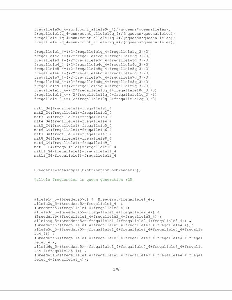
178
freqallele9q_4=sum(count_allele9q_4)/(nqueens*queenalleles); freqallele10q_4=sum(count_allele10q_4)/(nqueens*queenalleles); freqallele11q_4=sum(count_allele11q_4)/(nqueens*queenalleles); freqallele12q_4=sum(count_allele12q_4)/(nqueens*queenalleles);
freqallele1_4=((2*freqallele1q_4+freqallele1q_3)/3) freqallele2_4=((2*freqallele2q_4+freqallele2q_3)/3) freqallele3_4=((2*freqallele3q_4+freqallele3q_3)/3) freqallele4_4=((2*freqallele4q_4+freqallele4q_3)/3) freqallele5_4=((2*freqallele5q_4+freqallele5q_3)/3) freqallele6_4=((2*freqallele6q_4+freqallele6q_3)/3) freqallele7_4=((2*freqallele7q_4+freqallele7q_3)/3) freqallele8_4=((2*freqallele8q_4+freqallele8q_3)/3) freqallele9_4=((2*freqallele9q_4+freqallele9q_3)/3) freqallele10_4=((2*freqallele10q_4+freqallele10q_3)/3) freqallele11_4=((2*freqallele11q_4+freqallele11q_3)/3) freqallele12_4=((2*freqallele12q_4+freqallele12q_3)/3)
mat1_G4(freqallele1)=freqallele1_4 mat2_G4(freqallele1)=freqallele2_4 mat3_G4(freqallele1)=freqallele3_4 mat4_G4(freqallele1)=freqallele4_4 mat5_G4(freqallele1)=freqallele5_4 mat6_G4(freqallele1)=freqallele6_4 mat7_G4(freqallele1)=freqallele7_4 mat8_G4(freqallele1)=freqallele8_4 mat9_G4(freqallele1)=freqallele9_4 mat10_G4(freqallele1)=freqallele10_4 mat11_G4(freqallele1)=freqallele11_4 mat12_G4(freqallele1)=freqallele12_4
Breeders5=datasample(Distribution,nobreeders5);
%allele frequencies in queen generation (G5)
allele1q_5=(Breeders5>0) & (Breeders5<freqallele1_4); allele2q_5=(Breeders5>=freqallele1_4) &
(Breeders5<(freqallele1_4+freqallele2_4)); allele3q_5=(Breeders5>=(freqallele1_4+freqallele2_4)) &
(Breeders5<(freqallele1_4+freqallele2_4+freqallele3_4)); allele4q_5=(Breeders5>=(freqallele1_4+freqallele2_4+freqallele3_4)) &
(Breeders5<(freqallele1_4+freqallele2_4+freqallele3_4+freqallele4_4)); allele5q_5=(Breeders5>=(freqallele1_4+freqallele2_4+freqallele3_4+freqalle
le4_4)) &
(Breeders5<(freqallele1_4+freqallele2_4+freqallele3_4+freqallele4_4+freqal
lele5_4)); allele6q_5=(Breeders5>=(freqallele1_4+freqallele2_4+freqallele3_4+freqalle
le4_4+freqallele5_4)) &
(Breeders5<(freqallele1_4+freqallele2_4+freqallele3_4+freqallele4_4+freqal
lele5_4+freqallele6_4));

179
allele7q_5=(Breeders5>=(freqallele1_4+freqallele2_4+freqallele3_4+freqalle
le4_4+freqallele5_4+freqallele6_4)) &
(Breeders5<(freqallele1_4+freqallele2_4+freqallele3_4+freqallele4_4+freqal
lele5_4+freqallele6_4+freqallele7_4)); allele8q_5=(Breeders5>=(freqallele1_4+freqallele2_4+freqallele3_4+freqalle
le4_4+freqallele5_4+freqallele6_4+freqallele7_4)) &
(Breeders5<(freqallele1_4+freqallele2_4+freqallele3_4+freqallele4_4+freqal
lele5_4+freqallele6_4+freqallele7_4+freqallele8_4)); allele9q_5=(Breeders5>=(freqallele1_4+freqallele2_4+freqallele3_4+freqalle
le4_4+freqallele5_4+freqallele6_4+freqallele7_4+freqallele8_4)) &
(Breeders5<(freqallele1_4+freqallele2_4+freqallele3_4+freqallele4_4+freqal
lele5_4+freqallele6_4+freqallele7_4+freqallele8_4+freqallele9_4)); allele10q_5=(Breeders5>=(freqallele1_4+freqallele2_4+freqallele3_4+freqall
ele4_4+freqallele5_4+freqallele6_4+freqallele7_4+freqallele8_4+freqallele9
_4)) &
(Breeders5<(freqallele1_4+freqallele2_4+freqallele3_4+freqallele4_4+freqal
lele5_4+freqallele6_4+freqallele7_4+freqallele8_4+freqallele9_4+freqallele
10_4)); allele11q_5=(Breeders5>=(freqallele1_4+freqallele2_4+freqallele3_4+freqall
ele4_4+freqallele5_4+freqallele6_4+freqallele7_4+freqallele8_4+freqallele9
_4+freqallele10_4)) &
(Breeders5<(freqallele1_4+freqallele2_4+freqallele3_4+freqallele4_4+freqal
lele5_4+freqallele6_4+freqallele7_4+freqallele8_4+freqallele9_4+freqallele
10_4+freqallele11_4)); allele12q_5=(Breeders5>=(freqallele1_4+freqallele2_4+freqallele3_4+freqall
ele4_4+freqallele5_4+freqallele6_4+freqallele7_4+freqallele8_4+freqallele9
_4+freqallele10_4+freqallele11_4)) & (Breeders5<1.0);
count_allele1q_5=sum(allele1q_5); count_allele2q_5=sum(allele2q_5); count_allele3q_5=sum(allele3q_5); count_allele4q_5=sum(allele4q_5); count_allele5q_5=sum(allele5q_5); count_allele6q_5=sum(allele6q_5); count_allele7q_5=sum(allele7q_5); count_allele8q_5=sum(allele8q_5); count_allele9q_5=sum(allele9q_5); count_allele10q_5=sum(allele10q_5); count_allele11q_5=sum(allele11q_5); count_allele12q_5=sum(allele12q_5);
freqallele1q_5=sum(count_allele1q_5)/(nobreeders5*queenalleles); freqallele2q_5=sum(count_allele2q_5)/(nobreeders5*queenalleles); freqallele3q_5=sum(count_allele3q_5)/(nobreeders5*queenalleles); freqallele4q_5=sum(count_allele4q_5)/(nobreeders5*queenalleles); freqallele5q_5=sum(count_allele5q_5)/(nobreeders5*queenalleles); freqallele6q_5=sum(count_allele6q_5)/(nobreeders5*queenalleles); freqallele7q_5=sum(count_allele7q_5)/(nobreeders5*queenalleles); freqallele8q_5=sum(count_allele8q_5)/(nobreeders5*queenalleles); freqallele9q_5=sum(count_allele9q_5)/(nobreeders5*queenalleles); freqallele10q_5=sum(count_allele10q_5)/(nobreeders5*queenalleles); freqallele11q_5=sum(count_allele11q_5)/(nobreeders5*queenalleles); freqallele12q_5=sum(count_allele12q_5)/(nobreeders5*queenalleles);
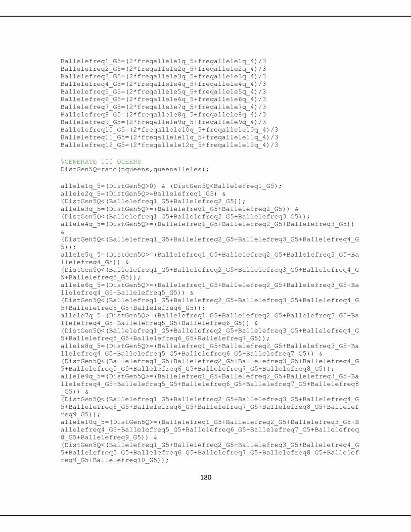
180
Ballelefreq1_G5=(2*freqallele1q_5+freqallele1q_4)/3 Ballelefreq2_G5=(2*freqallele2q_5+freqallele2q_4)/3 Ballelefreq3_G5=(2*freqallele3q_5+freqallele3q_4)/3 Ballelefreq4_G5=(2*freqallele4q_5+freqallele4q_4)/3 Ballelefreq5_G5=(2*freqallele5q_5+freqallele5q_4)/3 Ballelefreq6_G5=(2*freqallele6q_5+freqallele6q_4)/3 Ballelefreq7_G5=(2*freqallele7q_5+freqallele7q_4)/3 Ballelefreq8_G5=(2*freqallele8q_5+freqallele8q_4)/3 Ballelefreq9_G5=(2*freqallele9q_5+freqallele9q_4)/3 Ballelefreq10_G5=(2*freqallele10q_5+freqallele10q_4)/3 Ballelefreq11_G5=(2*freqallele11q_5+freqallele11q_4)/3 Ballelefreq12_G5=(2*freqallele12q_5+freqallele12q_4)/3
%GENERATE 100 QUEENS DistGen5Q=rand(nqueens,queenalleles);
allele1q_5=(DistGen5Q>0) & (DistGen5Q<Ballelefreq1_G5); allele2q_5=(DistGen5Q>=Ballelefreq1_G5) &
(DistGen5Q<(Ballelefreq1_G5+Ballelefreq2_G5)); allele3q_5=(DistGen5Q>=(Ballelefreq1_G5+Ballelefreq2_G5)) &
(DistGen5Q<(Ballelefreq1_G5+Ballelefreq2_G5+Ballelefreq3_G5)); allele4q_5=(DistGen5Q>=(Ballelefreq1_G5+Ballelefreq2_G5+Ballelefreq3_G5))
&
(DistGen5Q<(Ballelefreq1_G5+Ballelefreq2_G5+Ballelefreq3_G5+Ballelefreq4_G
5)); allele5q_5=(DistGen5Q>=(Ballelefreq1_G5+Ballelefreq2_G5+Ballelefreq3_G5+Ba
llelefreq4_G5)) &
(DistGen5Q<(Ballelefreq1_G5+Ballelefreq2_G5+Ballelefreq3_G5+Ballelefreq4_G
5+Ballelefreq5_G5)); allele6q_5=(DistGen5Q>=(Ballelefreq1_G5+Ballelefreq2_G5+Ballelefreq3_G5+Ba
llelefreq4_G5+Ballelefreq5_G5)) &
(DistGen5Q<(Ballelefreq1_G5+Ballelefreq2_G5+Ballelefreq3_G5+Ballelefreq4_G
5+Ballelefreq5_G5+Ballelefreq6_G5)); allele7q_5=(DistGen5Q>=(Ballelefreq1_G5+Ballelefreq2_G5+Ballelefreq3_G5+Ba
llelefreq4_G5+Ballelefreq5_G5+Ballelefreq6_G5)) &
(DistGen5Q<(Ballelefreq1_G5+Ballelefreq2_G5+Ballelefreq3_G5+Ballelefreq4_G
5+Ballelefreq5_G5+Ballelefreq6_G5+Ballelefreq7_G5)); allele8q_5=(DistGen5Q>=(Ballelefreq1_G5+Ballelefreq2_G5+Ballelefreq3_G5+Ba
llelefreq4_G5+Ballelefreq5_G5+Ballelefreq6_G5+Ballelefreq7_G5)) &
(DistGen5Q<(Ballelefreq1_G5+Ballelefreq2_G5+Ballelefreq3_G5+Ballelefreq4_G
5+Ballelefreq5_G5+Ballelefreq6_G5+Ballelefreq7_G5+Ballelefreq8_G5)); allele9q_5=(DistGen5Q>=(Ballelefreq1_G5+Ballelefreq2_G5+Ballelefreq3_G5+Ba
llelefreq4_G5+Ballelefreq5_G5+Ballelefreq6_G5+Ballelefreq7_G5+Ballelefreq8
_G5)) &
(DistGen5Q<(Ballelefreq1_G5+Ballelefreq2_G5+Ballelefreq3_G5+Ballelefreq4_G
5+Ballelefreq5_G5+Ballelefreq6_G5+Ballelefreq7_G5+Ballelefreq8_G5+Ballelef
req9_G5)); allele10q_5=(DistGen5Q>=(Ballelefreq1_G5+Ballelefreq2_G5+Ballelefreq3_G5+B
allelefreq4_G5+Ballelefreq5_G5+Ballelefreq6_G5+Ballelefreq7_G5+Ballelefreq
8_G5+Ballelefreq9_G5)) &
(DistGen5Q<(Ballelefreq1_G5+Ballelefreq2_G5+Ballelefreq3_G5+Ballelefreq4_G
5+Ballelefreq5_G5+Ballelefreq6_G5+Ballelefreq7_G5+Ballelefreq8_G5+Ballelef
req9_G5+Ballelefreq10_G5));

181
allele11q_5=(DistGen5Q>=(Ballelefreq1_G5+Ballelefreq2_G5+Ballelefreq3_G5+B
allelefreq4_G5+Ballelefreq5_G5+Ballelefreq6_G5+Ballelefreq7_G5+Ballelefreq
8_G5+Ballelefreq9_G5+Ballelefreq10_G5)) &
(DistGen5Q<(Ballelefreq1_G5+Ballelefreq2_G5+Ballelefreq3_G5+Ballelefreq4_G
5+Ballelefreq5_G5+Ballelefreq6_G5+Ballelefreq7_G5+Ballelefreq8_G5+Ballelef
req9_G5+Ballelefreq10_G5+Ballelefreq11_G5)); allele12q_5=(DistGen5Q>=(Ballelefreq1_G5+Ballelefreq2_G5+Ballelefreq3_G5+B
allelefreq4_G5+Ballelefreq5_G5+Ballelefreq6_G5+Ballelefreq7_G5+Ballelefreq
8_G5+Ballelefreq9_G5+Ballelefreq10_G5+Ballelefreq11_G5)) & (DistGen5Q<1);
count_allele1q_5=sum(allele1q_5); count_allele2q_5=sum(allele2q_5); count_allele3q_5=sum(allele3q_5); count_allele4q_5=sum(allele4q_5); count_allele5q_5=sum(allele5q_5); count_allele6q_5=sum(allele6q_5); count_allele7q_5=sum(allele7q_5); count_allele8q_5=sum(allele8q_5); count_allele9q_5=sum(allele9q_5); count_allele10q_5=sum(allele10q_5); count_allele11q_5=sum(allele11q_5); count_allele12q_5=sum(allele12q_5);
freqallele1q_5=sum(count_allele1q_5)/(nqueens*queenalleles); freqallele2q_5=sum(count_allele2q_5)/(nqueens*queenalleles); freqallele3q_5=sum(count_allele3q_5)/(nqueens*queenalleles); freqallele4q_5=sum(count_allele4q_5)/(nqueens*queenalleles); freqallele5q_5=sum(count_allele5q_5)/(nqueens*queenalleles); freqallele6q_5=sum(count_allele6q_5)/(nqueens*queenalleles); freqallele7q_5=sum(count_allele7q_5)/(nqueens*queenalleles); freqallele8q_5=sum(count_allele8q_5)/(nqueens*queenalleles); freqallele9q_5=sum(count_allele9q_5)/(nqueens*queenalleles); freqallele10q_5=sum(count_allele10q_5)/(nqueens*queenalleles); freqallele11q_5=sum(count_allele11q_5)/(nqueens*queenalleles); freqallele12q_5=sum(count_allele12q_5)/(nqueens*queenalleles);
freqallele1_5=((2*freqallele1q_5+freqallele1q_4)/3) freqallele2_5=((2*freqallele2q_5+freqallele2q_4)/3) freqallele3_5=((2*freqallele3q_5+freqallele3q_4)/3) freqallele4_5=((2*freqallele4q_5+freqallele4q_4)/3) freqallele5_5=((2*freqallele5q_5+freqallele5q_4)/3) freqallele6_5=((2*freqallele6q_5+freqallele6q_4)/3) freqallele7_5=((2*freqallele7q_5+freqallele7q_4)/3) freqallele8_5=((2*freqallele8q_5+freqallele8q_4)/3) freqallele9_5=((2*freqallele9q_5+freqallele9q_4)/3) freqallele10_5=((2*freqallele10q_5+freqallele10q_4)/3) freqallele11_5=((2*freqallele11q_5+freqallele11q_4)/3) freqallele12_5=((2*freqallele12q_5+freqallele12q_4)/3)
mat1_G5(freqallele1)=freqallele1_5 mat2_G5(freqallele1)=freqallele2_5 mat3_G5(freqallele1)=freqallele3_5 mat4_G5(freqallele1)=freqallele4_5 mat5_G5(freqallele1)=freqallele5_5

182
mat6_G5(freqallele1)=freqallele6_5 mat7_G5(freqallele1)=freqallele7_5 mat8_G5(freqallele1)=freqallele8_5 mat9_G5(freqallele1)=freqallele9_5 mat10_G5(freqallele1)=freqallele10_5 mat11_G5(freqallele1)=freqallele11_5 mat12_G5(freqallele1)=freqallele12_5 end
Matallele1=[mat1_G0; mat1_G1; mat1_G2; mat1_G3; mat1_G4; mat1_G5] Matallele2=[mat2_G0; mat2_G1; mat2_G2; mat2_G3; mat2_G4; mat2_G5] Matallele3=[mat3_G0; mat3_G1; mat3_G2; mat3_G3; mat3_G4; mat3_G5] Matallele4=[mat4_G0; mat4_G1; mat4_G2; mat4_G3; mat4_G4; mat4_G5] Matallele5=[mat5_G0; mat5_G1; mat5_G2; mat5_G3; mat5_G4; mat5_G5] Matallele6=[mat6_G0; mat6_G1; mat6_G2; mat6_G3; mat6_G4; mat6_G5] Matallele7=[mat7_G0; mat7_G1; mat7_G2; mat7_G3; mat7_G4; mat7_G5] Matallele8=[mat8_G0; mat8_G1; mat8_G2; mat8_G3; mat8_G4; mat8_G5] Matallele9=[mat9_G0; mat9_G1; mat9_G2; mat9_G3; mat9_G4; mat9_G5] Matallele10=[mat10_G0; mat10_G1; mat10_G2; mat10_G3; mat10_G4; mat10_G5] Matallele11=[mat11_G0; mat11_G1; mat11_G2; mat11_G3; mat11_G4; mat11_G5] Matallele12=[mat12_G0; mat12_G1; mat12_G2; mat12_G3; mat12_G4; mat12_G5]
Alldata=[Matallele1; Matallele2; Matallele3; Matallele4; Matallele5;
Matallele6; Matallele7; Matallele8; Matallele9; Matallele10; Matallele11;
Matallele12]
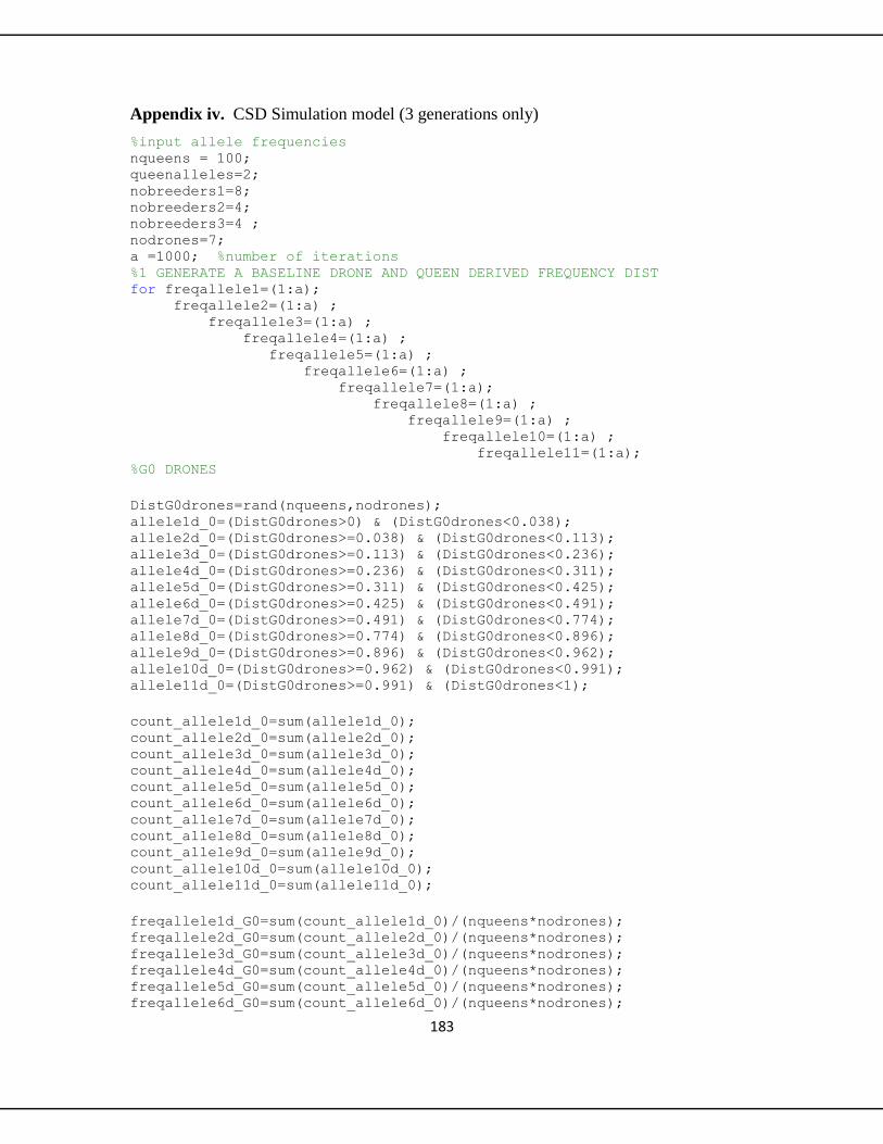
183
Appendix iv. CSD Simulation model (3 generations only)
%input allele frequencies nqueens = 100; queenalleles=2; nobreeders1=8; nobreeders2=4; nobreeders3=4 ; nodrones=7; a =1000; %number of iterations %1 GENERATE A BASELINE DRONE AND QUEEN DERIVED FREQUENCY DIST for freqallele1=(1:a); freqallele2=(1:a) ; freqallele3=(1:a) ; freqallele4=(1:a) ; freqallele5=(1:a) ; freqallele6=(1:a) ; freqallele7=(1:a); freqallele8=(1:a) ; freqallele9=(1:a) ; freqallele10=(1:a) ; freqallele11=(1:a); %G0 DRONES
DistG0drones=rand(nqueens,nodrones); allele1d_0=(DistG0drones>0) & (DistG0drones<0.038); allele2d_0=(DistG0drones>=0.038) & (DistG0drones<0.113); allele3d_0=(DistG0drones>=0.113) & (DistG0drones<0.236); allele4d_0=(DistG0drones>=0.236) & (DistG0drones<0.311); allele5d_0=(DistG0drones>=0.311) & (DistG0drones<0.425); allele6d_0=(DistG0drones>=0.425) & (DistG0drones<0.491); allele7d_0=(DistG0drones>=0.491) & (DistG0drones<0.774); allele8d_0=(DistG0drones>=0.774) & (DistG0drones<0.896); allele9d_0=(DistG0drones>=0.896) & (DistG0drones<0.962); allele10d_0=(DistG0drones>=0.962) & (DistG0drones<0.991); allele11d_0=(DistG0drones>=0.991) & (DistG0drones<1);
count_allele1d_0=sum(allele1d_0); count_allele2d_0=sum(allele2d_0); count_allele3d_0=sum(allele3d_0); count_allele4d_0=sum(allele4d_0); count_allele5d_0=sum(allele5d_0); count_allele6d_0=sum(allele6d_0); count_allele7d_0=sum(allele7d_0); count_allele8d_0=sum(allele8d_0); count_allele9d_0=sum(allele9d_0); count_allele10d_0=sum(allele10d_0); count_allele11d_0=sum(allele11d_0);
freqallele1d_G0=sum(count_allele1d_0)/(nqueens*nodrones); freqallele2d_G0=sum(count_allele2d_0)/(nqueens*nodrones); freqallele3d_G0=sum(count_allele3d_0)/(nqueens*nodrones); freqallele4d_G0=sum(count_allele4d_0)/(nqueens*nodrones); freqallele5d_G0=sum(count_allele5d_0)/(nqueens*nodrones); freqallele6d_G0=sum(count_allele6d_0)/(nqueens*nodrones);
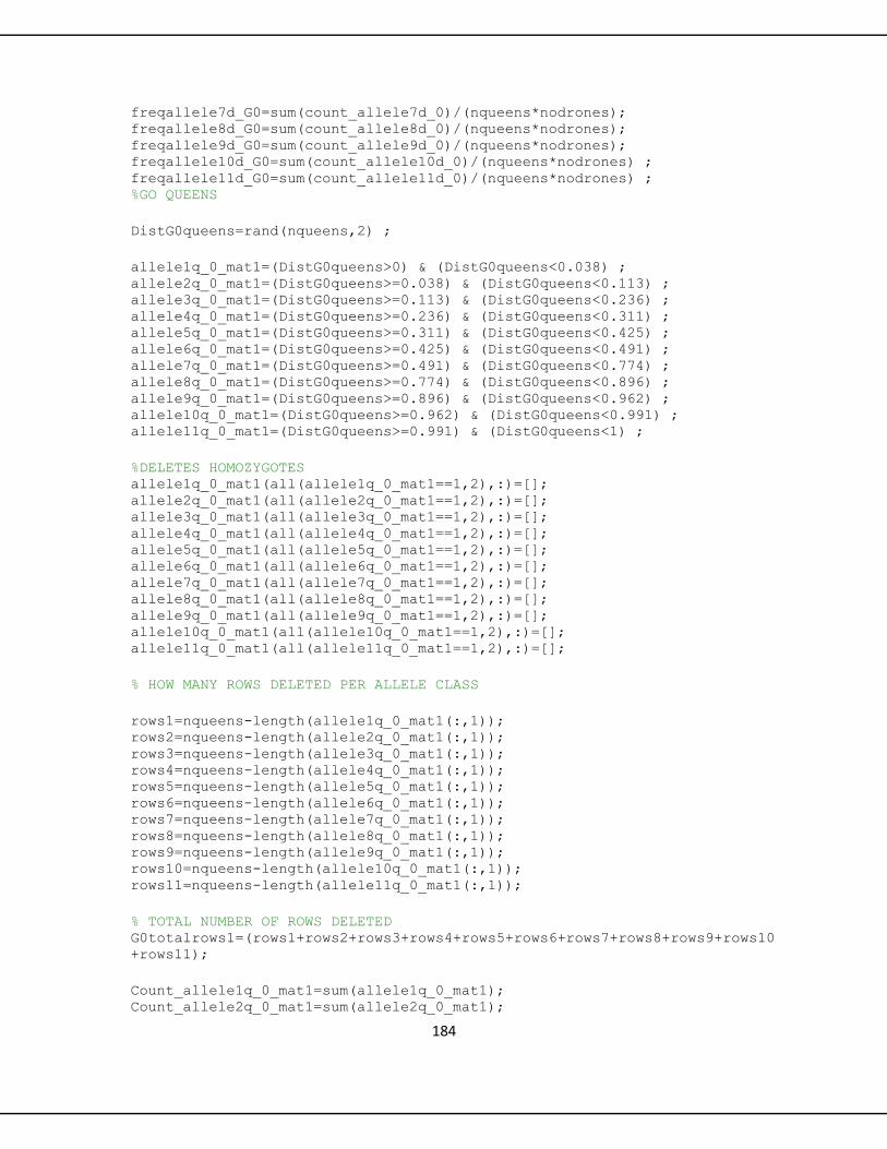
184
freqallele7d_G0=sum(count_allele7d_0)/(nqueens*nodrones); freqallele8d_G0=sum(count_allele8d_0)/(nqueens*nodrones); freqallele9d_G0=sum(count_allele9d_0)/(nqueens*nodrones); freqallele10d_G0=sum(count_allele10d_0)/(nqueens*nodrones) ; freqallele11d_G0=sum(count_allele11d_0)/(nqueens*nodrones) ; %GO QUEENS
DistG0queens=rand(nqueens,2) ;
allele1q_0_mat1=(DistG0queens>0) & (DistG0queens<0.038) ; allele2q_0_mat1=(DistG0queens>=0.038) & (DistG0queens<0.113) ; allele3q_0_mat1=(DistG0queens>=0.113) & (DistG0queens<0.236) ; allele4q_0_mat1=(DistG0queens>=0.236) & (DistG0queens<0.311) ; allele5q_0_mat1=(DistG0queens>=0.311) & (DistG0queens<0.425) ; allele6q_0_mat1=(DistG0queens>=0.425) & (DistG0queens<0.491) ; allele7q_0_mat1=(DistG0queens>=0.491) & (DistG0queens<0.774) ; allele8q_0_mat1=(DistG0queens>=0.774) & (DistG0queens<0.896) ; allele9q_0_mat1=(DistG0queens>=0.896) & (DistG0queens<0.962) ; allele10q_0_mat1=(DistG0queens>=0.962) & (DistG0queens<0.991) ; allele11q_0_mat1=(DistG0queens>=0.991) & (DistG0queens<1) ;
%DELETES HOMOZYGOTES allele1q_0_mat1(all(allele1q_0_mat1==1,2),:)=[]; allele2q_0_mat1(all(allele2q_0_mat1==1,2),:)=[]; allele3q_0_mat1(all(allele3q_0_mat1==1,2),:)=[]; allele4q_0_mat1(all(allele4q_0_mat1==1,2),:)=[]; allele5q_0_mat1(all(allele5q_0_mat1==1,2),:)=[]; allele6q_0_mat1(all(allele6q_0_mat1==1,2),:)=[]; allele7q_0_mat1(all(allele7q_0_mat1==1,2),:)=[]; allele8q_0_mat1(all(allele8q_0_mat1==1,2),:)=[]; allele9q_0_mat1(all(allele9q_0_mat1==1,2),:)=[]; allele10q_0_mat1(all(allele10q_0_mat1==1,2),:)=[]; allele11q_0_mat1(all(allele11q_0_mat1==1,2),:)=[];
% HOW MANY ROWS DELETED PER ALLELE CLASS
rows1=nqueens-length(allele1q_0_mat1(:,1)); rows2=nqueens-length(allele2q_0_mat1(:,1)); rows3=nqueens-length(allele3q_0_mat1(:,1)); rows4=nqueens-length(allele4q_0_mat1(:,1)); rows5=nqueens-length(allele5q_0_mat1(:,1)); rows6=nqueens-length(allele6q_0_mat1(:,1)); rows7=nqueens-length(allele7q_0_mat1(:,1)); rows8=nqueens-length(allele8q_0_mat1(:,1)); rows9=nqueens-length(allele9q_0_mat1(:,1)); rows10=nqueens-length(allele10q_0_mat1(:,1)); rows11=nqueens-length(allele11q_0_mat1(:,1));
% TOTAL NUMBER OF ROWS DELETED G0totalrows1=(rows1+rows2+rows3+rows4+rows5+rows6+rows7+rows8+rows9+rows10
+rows11);
Count_allele1q_0_mat1=sum(allele1q_0_mat1); Count_allele2q_0_mat1=sum(allele2q_0_mat1);

185
Count_allele3q_0_mat1=sum(allele3q_0_mat1); Count_allele4q_0_mat1=sum(allele4q_0_mat1); Count_allele5q_0_mat1=sum(allele5q_0_mat1); Count_allele6q_0_mat1=sum(allele6q_0_mat1); Count_allele7q_0_mat1=sum(allele7q_0_mat1); Count_allele8q_0_mat1=sum(allele8q_0_mat1); Count_allele9q_0_mat1=sum(allele9q_0_mat1); Count_allele10q_0_mat1=sum(allele10q_0_mat1); Count_allele11q_0_mat1=sum(allele11q_0_mat1);
freqallele1q_0_mat1=sum(Count_allele1q_0_mat1)/(nqueens*2) ; freqallele2q_0_mat1=sum(Count_allele2q_0_mat1)/(nqueens*2); freqallele3q_0_mat1=sum(Count_allele3q_0_mat1)/(nqueens*2) ; freqallele4q_0_mat1=sum(Count_allele4q_0_mat1)/(nqueens*2) ; freqallele5q_0_mat1=sum(Count_allele5q_0_mat1)/(nqueens*2) ; freqallele6q_0_mat1=sum(Count_allele6q_0_mat1)/(nqueens*2) ; freqallele7q_0_mat1=sum(Count_allele7q_0_mat1)/(nqueens*2) ; freqallele8q_0_mat1=sum(Count_allele8q_0_mat1)/(nqueens*2) ; freqallele9q_0_mat1=sum(Count_allele9q_0_mat1)/(nqueens*2) ; freqallele10q_0_mat1=sum(Count_allele10q_0_mat1)/(nqueens*2) ; freqallele11q_0_mat1=sum(Count_allele11q_0_mat1)/(nqueens*2) ;
%GENERATE NEW ARRAY EQUALIN SIZE TO RELACE REMOVED ROWS ABOVE
dist1= rand(G0totalrows1,2) ;
allele1q_0_mat2=(dist1>0) & (dist1<0.038); allele2q_0_mat2=(dist1>=0.038) & (dist1<0.113); allele3q_0_mat2=(dist1>=0.113) & (dist1<0.236); allele4q_0_mat2=(dist1>=0.236) & (dist1<0.311); allele5q_0_mat2=(dist1>0.311) & (dist1<0.425) ; allele6q_0_mat2=(dist1>=0.425) & (dist1<0.491); allele7q_0_mat2=(dist1>=0.491) & (dist1<0.774); allele8q_0_mat2=(dist1>=0.774) & (dist1<0.896) ; allele9q_0_mat2=(dist1>=0.896) & (dist1<0.962); allele10q_0_mat2=(dist1>=0.962) & (dist1<0.991); allele11q_0_mat2=(dist1>=0.991) & (dist1<1) ;
%PURGE FOR HOMO AGAIN allele1q_0_mat2(all(allele1q_0_mat2==1,2),:)=[]; allele2q_0_mat2(all(allele2q_0_mat2==1,2),:)=[] ; allele3q_0_mat2(all(allele3q_0_mat2==1,2),:)=[] ; allele4q_0_mat2(all(allele4q_0_mat2==1,2),:)=[] ; allele5q_0_mat2(all(allele5q_0_mat2==1,2),:)=[]; allele6q_0_mat2(all(allele6q_0_mat2==1,2),:)=[]; allele7q_0_mat2(all(allele7q_0_mat2==1,2),:)=[]; allele8q_0_mat2(all(allele8q_0_mat2==1,2),:)=[]; allele9q_0_mat2(all(allele9q_0_mat2==1,2),:)=[]; allele10q_0_mat2(all(allele10q_0_mat2==1,2),:)=[]; allele11q_0_mat2(all(allele11q_0_mat2==1,2),:)=[];
rows12=G0totalrows1-length(allele1q_0_mat2(:,1)); %allele1 in matrix2 rows13=G0totalrows1-length(allele2q_0_mat2(:,1)); %allele2 in matrix2 rows14=G0totalrows1-length(allele3q_0_mat2(:,1));
186
rows15=G0totalrows1-length(allele4q_0_mat2(:,1)); rows16=G0totalrows1-length(allele5q_0_mat2(:,1)); rows17=G0totalrows1-length(allele6q_0_mat2(:,1)); rows18=G0totalrows1-length(allele7q_0_mat2(:,1)); rows19=G0totalrows1-length(allele8q_0_mat2(:,1)); rows20=G0totalrows1-length(allele9q_0_mat2(:,1)); rows21=G0totalrows1-length(allele10q_0_mat2(:,1)); rows22=G0totalrows1-length(allele11q_0_mat2(:,1));
%TOTAL NUMBER OF ALLELES REMOVED FROM MATRIX 2 G0totalrows2=(rows12+rows13+rows14+rows15+rows16+rows17+rows18+rows19+rows
20+rows21+rows22);
Count_allele1q_0_mat2=sum(allele1q_0_mat2) ; Count_allele2q_0_mat2=sum(allele2q_0_mat2); Count_allele3q_0_mat2=sum(allele3q_0_mat2); Count_allele4q_0_mat2=sum(allele4q_0_mat2); Count_allele5q_0_mat2=sum(allele5q_0_mat2); Count_allele6q_0_mat2=sum(allele6q_0_mat2) ; Count_allele7q_0_mat2=sum(allele7q_0_mat2); Count_allele8q_0_mat2=sum(allele8q_0_mat2); Count_allele9q_0_mat2=sum(allele9q_0_mat2) ; Count_allele10q_0_mat2=sum(allele10q_0_mat2); Count_allele11q_0_mat2=sum(allele11q_0_mat2);
freqallele1q_0_mat2=sum(Count_allele1q_0_mat2)/(nqueens*2); freqallele2q_0_mat2=sum(Count_allele2q_0_mat2)/(nqueens*2) ; freqallele3q_0_mat2=sum(Count_allele3q_0_mat2)/(nqueens*2); freqallele4q_0_mat2=sum(Count_allele4q_0_mat2)/(nqueens*2); freqallele5q_0_mat2=sum(Count_allele5q_0_mat2)/(nqueens*2); freqallele6q_0_mat2=sum(Count_allele6q_0_mat2)/(nqueens*2); freqallele7q_0_mat2=sum(Count_allele7q_0_mat2)/(nqueens*2); freqallele8q_0_mat2=sum(Count_allele8q_0_mat2)/(nqueens*2); freqallele9q_0_mat2=sum(Count_allele9q_0_mat2)/(nqueens*2); freqallele10q_0_mat2=sum(Count_allele10q_0_mat2)/(nqueens*2); freqallele11q_0_mat2=sum(Count_allele11q_0_mat2)/(nqueens*2); dist2= rand(G0totalrows2,2) ;
allele1q_0_mat3=(dist2>0) & (dist2<0.038) ; allele2q_0_mat3=(dist2>=0.038) & (dist2<0.113); allele3q_0_mat3=(dist2>=0.113) & (dist2<0.236); allele4q_0_mat3=(dist2>=0.236) & (dist2<0.311); allele5q_0_mat3=(dist2>0.311) & (dist2<0.425) ; allele6q_0_mat3=(dist2>=0.425) & (dist2<0.491); allele7q_0_mat3=(dist2>=0.491) & (dist2<0.774); allele8q_0_mat3=(dist2>=0.774) & (dist2<0.896) ; allele9q_0_mat3=(dist2>=0.896) & (dist2<0.962); allele10q_0_mat3=(dist2>=0.962) & (dist2<0.991); allele11q_0_mat3=(dist2>=0.991) & (dist2<1) ;
allele1q_0_mat3(all(allele1q_0_mat3==1,2),:)=[] ; allele2q_0_mat3(all(allele2q_0_mat3==1,2),:)=[] ; allele3q_0_mat3(all(allele3q_0_mat3==1,2),:)=[] ; allele4q_0_mat3(all(allele4q_0_mat3==1,2),:)=[] ;

187
allele5q_0_mat3(all(allele5q_0_mat3==1,2),:)=[] ; allele6q_0_mat3(all(allele6q_0_mat3==1,2),:)=[] ; allele7q_0_mat3(all(allele7q_0_mat3==1,2),:)=[]; allele8q_0_mat3(all(allele8q_0_mat3==1,2),:)=[] ; allele9q_0_mat3(all(allele9q_0_mat3==1,2),:)=[] ; allele10q_0_mat3(all(allele10q_0_mat3==1,2),:)=[]; allele11q_0_mat3(all(allele11q_0_mat3==1,2),:)=[] ;
rows23=G0totalrows2-length(allele1q_0_mat3(:,1)); rows24=G0totalrows2-length(allele2q_0_mat3(:,1)) ; rows25=G0totalrows2-length(allele3q_0_mat3(:,1)) ; rows26=G0totalrows2-length(allele4q_0_mat3(:,1)) ; rows27=G0totalrows2-length(allele5q_0_mat3(:,1)) ; rows28=G0totalrows2-length(allele6q_0_mat3(:,1)) ; rows29=G0totalrows2-length(allele7q_0_mat3(:,1)) ; rows30=G0totalrows2-length(allele8q_0_mat3(:,1)) ; rows31=G0totalrows2-length(allele9q_0_mat3(:,1)) ; rows32=G0totalrows2-length(allele10q_0_mat3(:,1)) ; rows33=G0totalrows2-length(allele11q_0_mat3(:,1)) ;
G0totalrows3=(rows23+rows24+rows25+rows26+rows27+rows28+rows29+rows30+rows
31+rows32+rows33);
Count_allele1q_0_mat3=sum(allele1q_0_mat3); Count_allele2q_0_mat3=sum(allele2q_0_mat3) ; Count_allele3q_0_mat3=sum(allele3q_0_mat3); Count_allele4q_0_mat3=sum(allele4q_0_mat3); Count_allele5q_0_mat3=sum(allele5q_0_mat3) ; Count_allele6q_0_mat3=sum(allele6q_0_mat3) ; Count_allele7q_0_mat3=sum(allele7q_0_mat3) ; Count_allele8q_0_mat3=sum(allele8q_0_mat3) ; Count_allele9q_0_mat3=sum(allele9q_0_mat3) ; Count_allele10q_0_mat3=sum(allele10q_0_mat3) ; Count_allele11q_0_mat3=sum(allele11q_0_mat3) ;
freqallele1q_0_mat3=sum(Count_allele1q_0_mat3)/(nqueens*2); freqallele2q_0_mat3=sum(Count_allele2q_0_mat3)/(nqueens*2); freqallele3q_0_mat3=sum(Count_allele3q_0_mat3)/(nqueens*2); freqallele4q_0_mat3=sum(Count_allele4q_0_mat3)/(nqueens*2); freqallele5q_0_mat3=sum(Count_allele5q_0_mat3)/(nqueens*2); freqallele6q_0_mat3=sum(Count_allele6q_0_mat3)/(nqueens*2) ; freqallele7q_0_mat3=sum(Count_allele7q_0_mat3)/(nqueens*2) ; freqallele8q_0_mat3=sum(Count_allele8q_0_mat3)/(nqueens*2); freqallele9q_0_mat3=sum(Count_allele9q_0_mat3)/(nqueens*2) ; freqallele10q_0_mat3=sum(Count_allele10q_0_mat3)/(nqueens*2) ; freqallele11q_0_mat3=sum(Count_allele11q_0_mat3)/(nqueens*2);
dist3=rand(G0totalrows3,2);
allele1q_0_mat4=(dist3>0) & (dist3<0.038) ; allele2q_0_mat4=(dist3>=0.038) & (dist3<0.113) ; allele3q_0_mat4=(dist3>=0.113) & (dist3<0.236) ; allele4q_0_mat4=(dist3>=0.236) & (dist3<0.311) ; allele5q_0_mat4=(dist3>0.311) & (dist3<0.425) ;
188
allele6q_0_mat4=(dist3>=0.425) & (dist3<0.491) ; allele7q_0_mat4=(dist3>=0.491) & (dist3<0.774); allele8q_0_mat4=(dist3>=0.774) & (dist3<0.896) ; allele9q_0_mat4=(dist3>=0.896) & (dist3<0.962) ; allele10q_0_mat4=(dist3>=0.962) & (dist3<0.991); allele11q_0_mat4=(dist3>=0.991) & (dist3<1) ;
allele1q_0_mat4(all(allele1q_0_mat4==1,2),:)=[] ; allele2q_0_mat4(all(allele2q_0_mat4==1,2),:)=[] ; allele3q_0_mat4(all(allele3q_0_mat4==1,2),:)=[]; allele4q_0_mat4(all(allele4q_0_mat4==1,2),:)=[]; allele5q_0_mat4(all(allele5q_0_mat4==1,2),:)=[]; allele6q_0_mat4(all(allele6q_0_mat4==1,2),:)=[]; allele7q_0_mat4(all(allele7q_0_mat4==1,2),:)=[]; allele8q_0_mat4(all(allele8q_0_mat4==1,2),:)=[]; allele9q_0_mat4(all(allele9q_0_mat4==1,2),:)=[]; allele10q_0_mat4(all(allele10q_0_mat4==1,2),:)=[]; allele11q_0_mat4(all(allele11q_0_mat4==1,2),:)=[];
rows34=G0totalrows3-length(allele1q_0_mat4(:,1)); rows35=G0totalrows3-length(allele2q_0_mat4(:,1)); rows36=G0totalrows3-length(allele3q_0_mat4(:,1)); rows37=G0totalrows3-length(allele4q_0_mat4(:,1)); rows38=G0totalrows3-length(allele5q_0_mat4(:,1)); rows39=G0totalrows3-length(allele6q_0_mat4(:,1)); rows40=G0totalrows3-length(allele7q_0_mat4(:,1)); rows41=G0totalrows3-length(allele8q_0_mat4(:,1)); rows42=G0totalrows3-length(allele9q_0_mat4(:,1)); rows43=G0totalrows3-length(allele10q_0_mat4(:,1)); rows44=G0totalrows3-length(allele11q_0_mat4(:,1));
G0totalrows4=(rows34+rows35+rows36+rows37+rows38+rows39+rows40+rows41+rows
42+rows43+rows44);
Count_allele1q_0_mat4=sum(allele1q_0_mat4); Count_allele2q_0_mat4=sum(allele2q_0_mat4) ; Count_allele3q_0_mat4=sum(allele3q_0_mat4); Count_allele4q_0_mat4=sum(allele4q_0_mat4); Count_allele5q_0_mat4=sum(allele5q_0_mat4) ; Count_allele6q_0_mat4=sum(allele6q_0_mat4); Count_allele7q_0_mat4=sum(allele7q_0_mat4); Count_allele8q_0_mat4=sum(allele8q_0_mat4); Count_allele9q_0_mat4=sum(allele9q_0_mat4); Count_allele10q_0_mat4=sum(allele10q_0_mat4); Count_allele11q_0_mat4=sum(allele11q_0_mat4);
freqallele1q_0_mat4=sum(Count_allele1q_0_mat4)/(nqueens*2) ; freqallele2q_0_mat4=sum(Count_allele2q_0_mat4)/(nqueens*2); freqallele3q_0_mat4=sum(Count_allele3q_0_mat4)/(nqueens*2); freqallele4q_0_mat4=sum(Count_allele4q_0_mat4)/(nqueens*2); freqallele5q_0_mat4=sum(Count_allele5q_0_mat4)/(nqueens*2); freqallele6q_0_mat4=sum(Count_allele6q_0_mat4)/(nqueens*2); freqallele7q_0_mat4=sum(Count_allele7q_0_mat4)/(nqueens*2); freqallele8q_0_mat4=sum(Count_allele8q_0_mat4)/(nqueens*2);
189
freqallele9q_0_mat4=sum(Count_allele9q_0_mat4)/(nqueens*2); freqallele10q_0_mat4=sum(Count_allele10q_0_mat4)/(nqueens*2); freqallele11q_0_mat4=sum(Count_allele11q_0_mat4)/(nqueens*2);
dist4=rand(G0totalrows4,2) ;
allele1q_0_mat5=(dist4>0) & (dist4<0.038) ; allele2q_0_mat5=(dist4>=0.038) & (dist4<0.113) ; allele3q_0_mat5=(dist4>=0.113) & (dist4<0.236) ; allele4q_0_mat5=(dist4>=0.236) & (dist4<0.311) ; allele5q_0_mat5=(dist4>0.311) & (dist4<0.425) ; allele6q_0_mat5=(dist4>=0.425) & (dist4<0.491) ; allele7q_0_mat5=(dist4>=0.491) & (dist4<0.774); allele8q_0_mat5=(dist4>=0.774) & (dist4<0.896) ; allele9q_0_mat5=(dist4>=0.896) & (dist4<0.962) ; allele10q_0_mat5=(dist4>=0.962) & (dist4<0.991); allele11q_0_mat5=(dist4>=0.991) & (dist4<1) ;
allele1q_0_mat5(all(allele1q_0_mat5==1,2),:)=[] ; allele2q_0_mat5(all(allele2q_0_mat5==1,2),:)=[]; allele3q_0_mat5(all(allele3q_0_mat5==1,2),:)=[]; allele4q_0_mat5(all(allele4q_0_mat5==1,2),:)=[]; allele5q_0_mat5(all(allele5q_0_mat5==1,2),:)=[]; allele6q_0_mat5(all(allele6q_0_mat5==1,2),:)=[]; allele7q_0_mat5(all(allele7q_0_mat5==1,2),:)=[]; allele8q_0_mat5(all(allele8q_0_mat5==1,2),:)=[] ; allele9q_0_mat5(all(allele9q_0_mat5==1,2),:)=[]; allele10q_0_mat5(all(allele10q_0_mat5==1,2),:)=[]; allele11q_0_mat5(all(allele11q_0_mat5==1,2),:)=[] ;
rows45=G0totalrows4-length(allele1q_0_mat5(:,1)) ; rows46=G0totalrows4-length(allele2q_0_mat5(:,1)) ; rows47=G0totalrows4-length(allele3q_0_mat5(:,1)) ; rows48=G0totalrows4-length(allele4q_0_mat5(:,1)) ; rows49=G0totalrows4-length(allele5q_0_mat5(:,1)); rows50=G0totalrows4-length(allele6q_0_mat5(:,1)); rows51=G0totalrows4-length(allele7q_0_mat5(:,1)) ; rows52=G0totalrows4-length(allele8q_0_mat5(:,1)) ; rows53=G0totalrows4-length(allele9q_0_mat5(:,1)); rows54=G0totalrows4-length(allele10q_0_mat5(:,1)) ; rows55=G0totalrows4-length(allele11q_0_mat5(:,1)) ;
G0totalrows5=(rows45+rows46+rows47+rows48+rows49+rows50+rows51+rows52+rows
53+rows54+rows55);
Count_allele1q_0_mat5=sum(allele1q_0_mat5) ; Count_allele2q_0_mat5=sum(allele2q_0_mat5) ; Count_allele3q_0_mat5=sum(allele3q_0_mat5) ; Count_allele4q_0_mat5=sum(allele4q_0_mat5) ; Count_allele5q_0_mat5=sum(allele5q_0_mat5) ; Count_allele6q_0_mat5=sum(allele6q_0_mat5) ; Count_allele7q_0_mat5=sum(allele7q_0_mat5) ; Count_allele8q_0_mat5=sum(allele8q_0_mat5) ; Count_allele9q_0_mat5=sum(allele9q_0_mat5) ;
190
Count_allele10q_0_mat5=sum(allele10q_0_mat5) ; Count_allele11q_0_mat5=sum(allele11q_0_mat5) ;
freqallele1q_0_mat5=sum(Count_allele1q_0_mat5)/(nqueens*2) ; freqallele2q_0_mat5=sum(Count_allele2q_0_mat5)/(nqueens*2) ; freqallele3q_0_mat5=sum(Count_allele3q_0_mat5)/(nqueens*2) ; freqallele4q_0_mat5=sum(Count_allele4q_0_mat5)/(nqueens*2) ; freqallele5q_0_mat5=sum(Count_allele5q_0_mat5)/(nqueens*2) ; freqallele6q_0_mat5=sum(Count_allele6q_0_mat5)/(nqueens*2) ; freqallele7q_0_mat5=sum(Count_allele7q_0_mat5)/(nqueens*2) ; freqallele8q_0_mat5=sum(Count_allele8q_0_mat5)/(nqueens*2) ; freqallele9q_0_mat5=sum(Count_allele9q_0_mat5)/(nqueens*2) ; freqallele10q_0_mat5=sum(Count_allele10q_0_mat5)/(nqueens*2) ; freqallele11q_0_mat5=sum(Count_allele11q_0_mat5)/(nqueens*2) ;
freqallele1q_G0=freqallele1q_0_mat1+freqallele1q_0_mat2+freqallele1q_0_mat
3+freqallele1q_0_mat4+freqallele1q_0_mat5; freqallele2q_G0=freqallele2q_0_mat1+freqallele2q_0_mat2+freqallele2q_0_mat
3+freqallele2q_0_mat4+freqallele2q_0_mat5; freqallele3q_G0=freqallele3q_0_mat1+freqallele3q_0_mat2+freqallele3q_0_mat
3+freqallele3q_0_mat4+freqallele3q_0_mat5; freqallele4q_G0=freqallele4q_0_mat1+freqallele4q_0_mat2+freqallele4q_0_mat
3+freqallele4q_0_mat4+freqallele4q_0_mat5; freqallele5q_G0=freqallele5q_0_mat1+freqallele5q_0_mat2+freqallele5q_0_mat
3+freqallele5q_0_mat4+freqallele5q_0_mat5; freqallele6q_G0=freqallele6q_0_mat1+freqallele6q_0_mat2+freqallele6q_0_mat
3+freqallele6q_0_mat4+freqallele6q_0_mat5; freqallele7q_G0=freqallele7q_0_mat1+freqallele7q_0_mat2+freqallele7q_0_mat
3+freqallele7q_0_mat4+freqallele7q_0_mat5; freqallele8q_G0=freqallele8q_0_mat1+freqallele8q_0_mat2+freqallele8q_0_mat
3+freqallele8q_0_mat4+freqallele8q_0_mat5; freqallele9q_G0=freqallele9q_0_mat1+freqallele9q_0_mat2+freqallele9q_0_mat
3+freqallele9q_0_mat4+freqallele9q_0_mat5; freqallele10q_G0=freqallele10q_0_mat1+freqallele10q_0_mat2+freqallele10q_0
_mat3+freqallele10q_0_mat4+freqallele10q_0_mat5; freqallele11q_G0=freqallele11q_0_mat1+freqallele11q_0_mat2+freqallele11q_0
_mat3+freqallele11q_0_mat4+freqallele11q_0_mat5;
%FREQUENCY OF ALLELES IN SIMULATED GENERTION GO freqallele1_G0=((2*freqallele1q_G0+freqallele1d_G0)/3); freqallele2_G0=((2*freqallele2q_G0+freqallele2d_G0)/3); freqallele3_G0=((2*freqallele3q_G0+freqallele3d_G0)/3); freqallele4_G0=((2*freqallele4q_G0+freqallele4d_G0)/3); freqallele5_G0=((2*freqallele5q_G0+freqallele5d_G0)/3); freqallele6_G0=((2*freqallele6q_G0+freqallele6d_G0)/3); freqallele7_G0=((2*freqallele7q_G0+freqallele7d_G0)/3); freqallele8_G0=((2*freqallele8q_G0+freqallele8d_G0)/3); freqallele9_G0=((2*freqallele9q_G0+freqallele9d_G0)/3); freqallele10_G0=((2*freqallele10q_G0+freqallele10d_G0)/3); freqallele11_G0=((2*freqallele11q_G0+freqallele11d_G0)/3);
mat1_G0(freqallele1)=freqallele1_G0; mat2_G0(freqallele1)=freqallele2_G0; mat3_G0(freqallele1)=freqallele3_G0;
191
mat4_G0(freqallele1)=freqallele4_G0; mat5_G0(freqallele1)=freqallele5_G0; mat6_G0(freqallele1)=freqallele6_G0; mat7_G0(freqallele1)=freqallele7_G0; mat8_G0(freqallele1)=freqallele8_G0; mat9_G0(freqallele1)=freqallele9_G0; mat10_G0(freqallele1)=freqallele10_G0; mat11_G0(freqallele1)=freqallele11_G0;
%NOW DETERMINE ALLELE FREQ IN SELECTED BREEDERS 1
Distribution=rand(nqueens,2); Breeders1=datasample(Distribution,nobreeders1);
allele1q_b1_mat1=(Breeders1>0) & (Breeders1<freqallele1_G0); allele2q_b1_mat1=(Breeders1>=freqallele1_G0) &
(Breeders1<(freqallele1_G0+freqallele2_G0)); allele3q_b1_mat1=(Breeders1>=(freqallele1_G0+freqallele2_G0)) &
(Breeders1<(freqallele1_G0+freqallele2_G0+freqallele3_G0)); allele4q_b1_mat1=(Breeders1>=(freqallele1_G0+freqallele2_G0+freqallele3_G0
)) &
(Breeders1<(freqallele1_G0+freqallele2_G0+freqallele3_G0+freqallele4_G0)); allele5q_b1_mat1=(Breeders1>=(freqallele1_G0+freqallele2_G0+freqallele3_G0
+freqallele4_G0)) &
(Breeders1<(freqallele1_G0+freqallele2_G0+freqallele3_G0+freqallele4_G0+fr
eqallele5_G0)); allele6q_b1_mat1=(Breeders1>=(freqallele1_G0+freqallele2_G0+freqallele3_G0
+freqallele4_G0+freqallele5_G0)) &
(Breeders1<(freqallele1_G0+freqallele2_G0+freqallele3_G0+freqallele4_G0+fr
eqallele5_G0+freqallele6_G0)); allele7q_b1_mat1=(Breeders1>=(freqallele1_G0+freqallele2_G0+freqallele3_G0
+freqallele4_G0+freqallele5_G0+freqallele6_G0)) &
(Breeders1<(freqallele1_G0+freqallele2_G0+freqallele3_G0+freqallele4_G0+fr
eqallele5_G0+freqallele6_G0+ freqallele7_G0)); allele8q_b1_mat1=(Breeders1>=(freqallele1_G0+freqallele2_G0+freqallele3_G0
+freqallele4_G0+freqallele5_G0+freqallele6_G0+ freqallele7_G0)) &
(Breeders1<(freqallele1_G0+freqallele2_G0+freqallele3_G0+freqallele4_G0+fr
eqallele5_G0+freqallele6_G0+ freqallele7_G0+freqallele8_G0)); allele9q_b1_mat1=(Breeders1>=(freqallele1_G0+freqallele2_G0+freqallele3_G0
+freqallele4_G0+freqallele5_G0+freqallele6_G0+
freqallele7_G0+freqallele8_G0)) &
(Breeders1<(freqallele1_G0+freqallele2_G0+freqallele3_G0+freqallele4_G0+fr
eqallele5_G0+freqallele6_G0+
freqallele7_G0+freqallele8_G0+freqallele9_G0)); allele10q_b1_mat1=(Breeders1>=(freqallele1_G0+freqallele2_G0+freqallele3_G
0+freqallele4_G0+freqallele5_G0+freqallele6_G0+
freqallele7_G0+freqallele8_G0+freqallele9_G0)) &
(Breeders1<(freqallele1_G0+freqallele2_G0+freqallele3_G0+freqallele4_G0+fr
eqallele5_G0+freqallele6_G0+
freqallele7_G0+freqallele8_G0+freqallele9_G0+freqallele10_G0));
192
allele11q_b1_mat1=(Breeders1>=(freqallele1_G0+freqallele2_G0+freqallele3_G
0+freqallele4_G0+freqallele5_G0+freqallele6_G0+
freqallele7_G0+freqallele8_G0+freqallele9_G0+freqallele10_G0)) &
(Breeders1<1);
%PURGE HOMOZYGOTES SELECTED AT RANDOM allele1q_b1_mat1(all(allele1q_b1_mat1==1,2),:)=[] ; allele2q_b1_mat1(all(allele2q_b1_mat1==1,2),:)=[] ; allele3q_b1_mat1(all(allele3q_b1_mat1==1,2),:)=[] ; allele4q_b1_mat1(all(allele4q_b1_mat1==1,2),:)=[] ; allele5q_b1_mat1(all(allele5q_b1_mat1==1,2),:)=[] ; allele6q_b1_mat1(all(allele6q_b1_mat1==1,2),:)=[] ; allele7q_b1_mat1(all(allele7q_b1_mat1==1,2),:)=[] ; allele8q_b1_mat1(all(allele8q_b1_mat1==1,2),:)=[] ; allele9q_b1_mat1(all(allele9q_b1_mat1==1,2),:)=[] ; allele10q_b1_mat1(all(allele10q_b1_mat1==1,2),:)=[]; allele11q_b1_mat1(all(allele11q_b1_mat1==1,2),:)=[];
rows1=nobreeders1-length(allele1q_b1_mat1(:,1)); rows2=nobreeders1-length(allele2q_b1_mat1(:,1)); rows3=nobreeders1-length(allele3q_b1_mat1(:,1)); rows4=nobreeders1-length(allele4q_b1_mat1(:,1)); rows5=nobreeders1-length(allele5q_b1_mat1(:,1)); rows6=nobreeders1-length(allele6q_b1_mat1(:,1)); rows7=nobreeders1-length(allele7q_b1_mat1(:,1)); rows8=nobreeders1-length(allele8q_b1_mat1(:,1)); rows9=nobreeders1-length(allele9q_b1_mat1(:,1)); rows10=nobreeders1-length(allele10q_b1_mat1(:,1)); rows11=nobreeders1-length(allele11q_b1_mat1(:,1));
G0totalrowsbreeders1=(rows1+rows2+rows3+rows4+rows5+rows6+rows7+rows8+rows
9+rows10+rows11);
count_allele1q_b1_mat1=sum(allele1q_b1_mat1); count_allele2q_b1_mat1=sum(allele2q_b1_mat1); count_allele3q_b1_mat1=sum(allele3q_b1_mat1); count_allele4q_b1_mat1=sum(allele4q_b1_mat1); count_allele5q_b1_mat1=sum(allele5q_b1_mat1); count_allele6q_b1_mat1=sum(allele6q_b1_mat1); count_allele7q_b1_mat1=sum(allele7q_b1_mat1); count_allele8q_b1_mat1=sum(allele8q_b1_mat1); count_allele9q_b1_mat1=sum(allele9q_b1_mat1); count_allele10q_b1_mat1=sum(allele10q_b1_mat1); count_allele11q_b1_mat1=sum(allele11q_b1_mat1);
freqallele1q_b1_mat1=sum(count_allele1q_b1_mat1)/(nobreeders1*2); freqallele2q_b1_mat1=sum(count_allele2q_b1_mat1)/(nobreeders1*2); freqallele3q_b1_mat1=sum(count_allele3q_b1_mat1)/(nobreeders1*2); freqallele4q_b1_mat1=sum(count_allele4q_b1_mat1)/(nobreeders1*2); freqallele5q_b1_mat1=sum(count_allele5q_b1_mat1)/(nobreeders1*2); freqallele6q_b1_mat1=sum(count_allele6q_b1_mat1)/(nobreeders1*2); freqallele7q_b1_mat1=sum(count_allele7q_b1_mat1)/(nobreeders1*2); freqallele8q_b1_mat1=sum(count_allele8q_b1_mat1)/(nobreeders1*2);
193
freqallele9q_b1_mat1=sum(count_allele9q_b1_mat1)/(nobreeders1*2); freqallele10q_b1_mat1=sum(count_allele10q_b1_mat1)/(nobreeders1*2); freqallele11q_b1_mat1=sum(count_allele11q_b1_mat1)/(nobreeders1*2);
dist1=rand(G0totalrowsbreeders1,2);
allele1q_b1_mat2=(dist1>0) & (dist1<freqallele1_G0); allele2q_b1_mat2=(dist1>=freqallele1_G0) &
(dist1<(freqallele1_G0+freqallele2_G0)); allele3q_b1_mat2=(dist1>=(freqallele1_G0+freqallele2_G0)) &
(dist1<(freqallele1_G0+freqallele2_G0+freqallele3_G0)); allele4q_b1_mat2=(dist1>=(freqallele1_G0+freqallele2_G0+freqallele3_G0)) &
(dist1<(freqallele1_G0+freqallele2_G0+freqallele3_G0+freqallele4_G0)); allele5q_b1_mat2=(dist1>=(freqallele1_G0+freqallele2_G0+freqallele3_G0+fre
qallele4_G0)) &
(dist1<(freqallele1_G0+freqallele2_G0+freqallele3_G0+freqallele4_G0+freqal
lele5_G0)); allele6q_b1_mat2=(dist1>=(freqallele1_G0+freqallele2_G0+freqallele3_G0+fre
qallele4_G0+freqallele5_G0)) &
(dist1<(freqallele1_G0+freqallele2_G0+freqallele3_G0+freqallele4_G0+freqal
lele5_G0+freqallele6_G0)); allele7q_b1_mat2=(dist1>=(freqallele1_G0+freqallele2_G0+freqallele3_G0+fre
qallele4_G0+freqallele5_G0+freqallele6_G0)) &
(dist1<(freqallele1_G0+freqallele2_G0+freqallele3_G0+freqallele4_G0+freqal
lele5_G0+freqallele6_G0+ freqallele7_G0)); allele8q_b1_mat2=(dist1>=(freqallele1_G0+freqallele2_G0+freqallele3_G0+fre
qallele4_G0+freqallele5_G0+freqallele6_G0+ freqallele7_G0)) &
(dist1<(freqallele1_G0+freqallele2_G0+freqallele3_G0+freqallele4_G0+freqal
lele5_G0+freqallele6_G0+ freqallele7_G0+freqallele8_G0)); allele9q_b1_mat2=(dist1>=(freqallele1_G0+freqallele2_G0+freqallele3_G0+fre
qallele4_G0+freqallele5_G0+freqallele6_G0+ freqallele7_G0+freqallele8_G0))
&
(dist1<(freqallele1_G0+freqallele2_G0+freqallele3_G0+freqallele4_G0+freqal
lele5_G0+freqallele6_G0+ freqallele7_G0+freqallele8_G0+freqallele9_G0)); allele10q_b1_mat2=(dist1>=(freqallele1_G0+freqallele2_G0+freqallele3_G0+fr
eqallele4_G0+freqallele5_G0+freqallele6_G0+
freqallele7_G0+freqallele8_G0+freqallele9_G0)) &
(dist1<(freqallele1_G0+freqallele2_G0+freqallele3_G0+freqallele4_G0+freqal
lele5_G0+freqallele6_G0+
freqallele7_G0+freqallele8_G0+freqallele9_G0+freqallele10_G0)); allele11q_b1_mat2=(dist1>=(freqallele1_G0+freqallele2_G0+freqallele3_G0+fr
eqallele4_G0+freqallele5_G0+freqallele6_G0+
freqallele7_G0+freqallele8_G0+freqallele9_G0+freqallele10_G0)) &
(dist1<1);
allele1q_b1_mat2(all(allele1q_b1_mat2==1,2),:)=[] ; allele2q_b1_mat2(all(allele2q_b1_mat2==1,2),:)=[] ; allele3q_b1_mat2(all(allele3q_b1_mat2==1,2),:)=[] ; allele4q_b1_mat2(all(allele4q_b1_mat2==1,2),:)=[] ; allele5q_b1_mat2(all(allele5q_b1_mat2==1,2),:)=[] ; allele6q_b1_mat2(all(allele6q_b1_mat2==1,2),:)=[] ; allele7q_b1_mat2(all(allele7q_b1_mat2==1,2),:)=[] ; allele8q_b1_mat2(all(allele8q_b1_mat2==1,2),:)=[] ; allele9q_b1_mat2(all(allele9q_b1_mat2==1,2),:)=[] ; allele10q_b1_mat2(all(allele10q_b1_mat2==1,2),:)=[] ;
194
allele11q_b1_mat2(all(allele11q_b1_mat2==1,2),:)=[] ;
rows12=G0totalrowsbreeders1-length(allele1q_b1_mat2(:,1)); rows13=G0totalrowsbreeders1-length(allele2q_b1_mat2(:,1)); rows14=G0totalrowsbreeders1-length(allele3q_b1_mat2(:,1)); rows15=G0totalrowsbreeders1-length(allele4q_b1_mat2(:,1)); rows16=G0totalrowsbreeders1-length(allele5q_b1_mat2(:,1)); rows17=G0totalrowsbreeders1-length(allele6q_b1_mat2(:,1)); rows18=G0totalrowsbreeders1-length(allele7q_b1_mat2(:,1)); rows19=G0totalrowsbreeders1-length(allele8q_b1_mat2(:,1)); rows20=G0totalrowsbreeders1-length(allele9q_b1_mat2(:,1)); rows21=G0totalrowsbreeders1-length(allele10q_b1_mat2(:,1)); rows22=G0totalrowsbreeders1-length(allele11q_b1_mat2(:,1));
G0totalrowsbreeders2=(rows12+rows13+rows14+rows15+rows16+rows17+rows18+row
s19+rows20+rows21+rows22);
count_allele1q_b1_mat2=sum(allele1q_b1_mat2); count_allele2q_b1_mat2=sum(allele2q_b1_mat2); count_allele3q_b1_mat2=sum(allele3q_b1_mat2); count_allele4q_b1_mat2=sum(allele4q_b1_mat2); count_allele5q_b1_mat2=sum(allele5q_b1_mat2); count_allele6q_b1_mat2=sum(allele6q_b1_mat2); count_allele7q_b1_mat2=sum(allele7q_b1_mat2); count_allele8q_b1_mat2=sum(allele8q_b1_mat2); count_allele9q_b1_mat2=sum(allele9q_b1_mat2); count_allele10q_b1_mat2=sum(allele10q_b1_mat2); count_allele11q_b1_mat2=sum(allele11q_b1_mat2);
freqallele1q_b1_mat2=sum(count_allele1q_b1_mat2)/(nobreeders1*2); freqallele2q_b1_mat2=sum(count_allele2q_b1_mat2)/(nobreeders1*2); freqallele3q_b1_mat2=sum(count_allele3q_b1_mat2)/(nobreeders1*2); freqallele4q_b1_mat2=sum(count_allele4q_b1_mat2)/(nobreeders1*2); freqallele5q_b1_mat2=sum(count_allele5q_b1_mat2)/(nobreeders1*2); freqallele6q_b1_mat2=sum(count_allele6q_b1_mat2)/(nobreeders1*2); freqallele7q_b1_mat2=sum(count_allele7q_b1_mat2)/(nobreeders1*2); freqallele8q_b1_mat2=sum(count_allele8q_b1_mat2)/(nobreeders1*2); freqallele9q_b1_mat2=sum(count_allele9q_b1_mat2)/(nobreeders1*2); freqallele10q_b1_mat2=sum(count_allele10q_b1_mat2)/(nobreeders1*2); freqallele11q_b1_mat2=sum(count_allele11q_b1_mat2)/(nobreeders1*2);
dist2=rand(G0totalrowsbreeders2,2);
allele1q_b1_mat3=(dist2>0) & (dist2<freqallele1_G0); allele2q_b1_mat3=(dist2>=freqallele1_G0) &
(dist2<(freqallele1_G0+freqallele2_G0)); allele3q_b1_mat3=(dist2>=(freqallele1_G0+freqallele2_G0)) &
(dist2<(freqallele1_G0+freqallele2_G0+freqallele3_G0)); allele4q_b1_mat3=(dist2>=(freqallele1_G0+freqallele2_G0+freqallele3_G0)) &
(dist2<(freqallele1_G0+freqallele2_G0+freqallele3_G0+freqallele4_G0)); allele5q_b1_mat3=(dist2>=(freqallele1_G0+freqallele2_G0+freqallele3_G0+fre
qallele4_G0)) &
(dist2<(freqallele1_G0+freqallele2_G0+freqallele3_G0+freqallele4_G0+freqal
lele5_G0));
195
allele6q_b1_mat3=(dist2>=(freqallele1_G0+freqallele2_G0+freqallele3_G0+fre
qallele4_G0+freqallele5_G0)) &
(dist2<(freqallele1_G0+freqallele2_G0+freqallele3_G0+freqallele4_G0+freqal
lele5_G0+freqallele6_G0)); allele7q_b1_mat3=(dist2>=(freqallele1_G0+freqallele2_G0+freqallele3_G0+fre
qallele4_G0+freqallele5_G0+freqallele6_G0)) &
(dist2<(freqallele1_G0+freqallele2_G0+freqallele3_G0+freqallele4_G0+freqal
lele5_G0+freqallele6_G0+ freqallele7_G0)); allele8q_b1_mat3=(dist2>=(freqallele1_G0+freqallele2_G0+freqallele3_G0+fre
qallele4_G0+freqallele5_G0+freqallele6_G0+ freqallele7_G0)) &
(dist2<(freqallele1_G0+freqallele2_G0+freqallele3_G0+freqallele4_G0+freqal
lele5_G0+freqallele6_G0+ freqallele7_G0+freqallele8_G0)); allele9q_b1_mat3=(dist2>=(freqallele1_G0+freqallele2_G0+freqallele3_G0+fre
qallele4_G0+freqallele5_G0+freqallele6_G0+ freqallele7_G0+freqallele8_G0))
&
(dist2<(freqallele1_G0+freqallele2_G0+freqallele3_G0+freqallele4_G0+freqal
lele5_G0+freqallele6_G0+ freqallele7_G0+freqallele8_G0+freqallele9_G0)); allele10q_b1_mat3=(dist2>=(freqallele1_G0+freqallele2_G0+freqallele3_G0+fr
eqallele4_G0+freqallele5_G0+freqallele6_G0+
freqallele7_G0+freqallele8_G0+freqallele9_G0)) &
(dist2<(freqallele1_G0+freqallele2_G0+freqallele3_G0+freqallele4_G0+freqal
lele5_G0+freqallele6_G0+
freqallele7_G0+freqallele8_G0+freqallele9_G0+freqallele10_G0)); allele11q_b1_mat3=(dist2>=(freqallele1_G0+freqallele2_G0+freqallele3_G0+fr
eqallele4_G0+freqallele5_G0+freqallele6_G0+
freqallele7_G0+freqallele8_G0+freqallele9_G0+freqallele10_G0)) &
(dist2<1);
allele1q_b1_mat3(all(allele1q_b1_mat3==1,2),:)=[] ; allele2q_b1_mat3(all(allele2q_b1_mat3==1,2),:)=[] ; allele3q_b1_mat3(all(allele3q_b1_mat3==1,2),:)=[] ; allele4q_b1_mat3(all(allele4q_b1_mat3==1,2),:)=[] ; allele5q_b1_mat3(all(allele5q_b1_mat3==1,2),:)=[] ; allele6q_b1_mat3(all(allele6q_b1_mat3==1,2),:)=[] ; allele7q_b1_mat3(all(allele7q_b1_mat3==1,2),:)=[] ; allele8q_b1_mat3(all(allele8q_b1_mat3==1,2),:)=[] ; allele9q_b1_mat3(all(allele9q_b1_mat3==1,2),:)=[] ; allele10q_b1_mat3(all(allele10q_b1_mat3==1,2),:)=[] ; allele11q_b1_mat3(all(allele11q_b1_mat3==1,2),:)=[] ;
rows23=G0totalrowsbreeders2-length(allele1q_b1_mat3(:,1)) ; rows24=G0totalrowsbreeders2-length(allele2q_b1_mat3(:,1)) ; rows25=G0totalrowsbreeders2-length(allele3q_b1_mat3(:,1)) ; rows26=G0totalrowsbreeders2-length(allele4q_b1_mat3(:,1)) ; rows27=G0totalrowsbreeders2-length(allele5q_b1_mat3(:,1)) ; rows28=G0totalrowsbreeders2-length(allele6q_b1_mat3(:,1)) ; rows29=G0totalrowsbreeders2-length(allele7q_b1_mat3(:,1)) ; rows30=G0totalrowsbreeders2-length(allele8q_b1_mat3(:,1)) ; rows31=G0totalrowsbreeders2-length(allele9q_b1_mat3(:,1)) ; rows32=G0totalrowsbreeders2-length(allele10q_b1_mat3(:,1)) ; rows33=G0totalrowsbreeders2-length(allele11q_b1_mat3(:,1)) ;
G0totalrowsbreeders3=(rows23+rows24+rows25+rows26+rows27+rows28+rows29+row
s30+rows31+rows32+rows33);
196
count_allele1q_b1_mat3=sum(allele1q_b1_mat3) ; count_allele2q_b1_mat3=sum(allele2q_b1_mat3) ; count_allele3q_b1_mat3=sum(allele3q_b1_mat3) ; count_allele4q_b1_mat3=sum(allele4q_b1_mat3) ; count_allele5q_b1_mat3=sum(allele5q_b1_mat3) ; count_allele6q_b1_mat3=sum(allele6q_b1_mat3) ; count_allele7q_b1_mat3=sum(allele7q_b1_mat3) ; count_allele8q_b1_mat3=sum(allele8q_b1_mat3) ; count_allele9q_b1_mat3=sum(allele9q_b1_mat3) ; count_allele10q_b1_mat3=sum(allele10q_b1_mat3) ; count_allele11q_b1_mat3=sum(allele11q_b1_mat3) ;
freqallele1q_b1_mat3=sum(count_allele1q_b1_mat3)/(nobreeders1*2) ; freqallele2q_b1_mat3=sum(count_allele2q_b1_mat3)/(nobreeders1*2) ; freqallele3q_b1_mat3=sum(count_allele3q_b1_mat3)/(nobreeders1*2) ; freqallele4q_b1_mat3=sum(count_allele4q_b1_mat3)/(nobreeders1*2) ; freqallele5q_b1_mat3=sum(count_allele5q_b1_mat3)/(nobreeders1*2) ; freqallele6q_b1_mat3=sum(count_allele6q_b1_mat3)/(nobreeders1*2) ; freqallele7q_b1_mat3=sum(count_allele7q_b1_mat3)/(nobreeders1*2) ; freqallele8q_b1_mat3=sum(count_allele8q_b1_mat3)/(nobreeders1*2) ; freqallele9q_b1_mat3=sum(count_allele9q_b1_mat3)/(nobreeders1*2) ; freqallele10q_b1_mat3=sum(count_allele10q_b1_mat3)/(nobreeders1*2) ; freqallele11q_b1_mat3=sum(count_allele11q_b1_mat3)/(nobreeders1*2) ;
dist3=rand(G0totalrowsbreeders3,2);
allele1q_b1_mat4=(dist3>0) & (dist3<freqallele1_G0); allele2q_b1_mat4=(dist3>=freqallele1_G0) &
(dist3<(freqallele1_G0+freqallele2_G0)); allele3q_b1_mat4=(dist3>=(freqallele1_G0+freqallele2_G0)) &
(dist3<(freqallele1_G0+freqallele2_G0+freqallele3_G0)); allele4q_b1_mat4=(dist3>=(freqallele1_G0+freqallele2_G0+freqallele3_G0)) &
(dist3<(freqallele1_G0+freqallele2_G0+freqallele3_G0+freqallele4_G0)); allele5q_b1_mat4=(dist3>=(freqallele1_G0+freqallele2_G0+freqallele3_G0+fre
qallele4_G0)) &
(dist3<(freqallele1_G0+freqallele2_G0+freqallele3_G0+freqallele4_G0+freqal
lele5_G0)); allele6q_b1_mat4=(dist3>=(freqallele1_G0+freqallele2_G0+freqallele3_G0+fre
qallele4_G0+freqallele5_G0)) &
(dist3<(freqallele1_G0+freqallele2_G0+freqallele3_G0+freqallele4_G0+freqal
lele5_G0+freqallele6_G0)); allele7q_b1_mat4=(dist3>=(freqallele1_G0+freqallele2_G0+freqallele3_G0+fre
qallele4_G0+freqallele5_G0+freqallele6_G0)) &
(dist3<(freqallele1_G0+freqallele2_G0+freqallele3_G0+freqallele4_G0+freqal
lele5_G0+freqallele6_G0+ freqallele7_G0)); allele8q_b1_mat4=(dist3>=(freqallele1_G0+freqallele2_G0+freqallele3_G0+fre
qallele4_G0+freqallele5_G0+freqallele6_G0+ freqallele7_G0)) &
(dist3<(freqallele1_G0+freqallele2_G0+freqallele3_G0+freqallele4_G0+freqal
lele5_G0+freqallele6_G0+ freqallele7_G0+freqallele8_G0)); allele9q_b1_mat4=(dist3>=(freqallele1_G0+freqallele2_G0+freqallele3_G0+fre
qallele4_G0+freqallele5_G0+freqallele6_G0+ freqallele7_G0+freqallele8_G0))
&

197
(dist3<(freqallele1_G0+freqallele2_G0+freqallele3_G0+freqallele4_G0+freqal
lele5_G0+freqallele6_G0+ freqallele7_G0+freqallele8_G0+freqallele9_G0)); allele10q_b1_mat4=(dist3>=(freqallele1_G0+freqallele2_G0+freqallele3_G0+fr
eqallele4_G0+freqallele5_G0+freqallele6_G0+
freqallele7_G0+freqallele8_G0+freqallele9_G0)) &
(dist3<(freqallele1_G0+freqallele2_G0+freqallele3_G0+freqallele4_G0+freqal
lele5_G0+freqallele6_G0+
freqallele7_G0+freqallele8_G0+freqallele9_G0+freqallele10_G0)); allele11q_b1_mat4=(dist3>=(freqallele1_G0+freqallele2_G0+freqallele3_G0+fr
eqallele4_G0+freqallele5_G0+freqallele6_G0+
freqallele7_G0+freqallele8_G0+freqallele9_G0+freqallele10_G0)) &
(dist3<1);
allele1q_b1_mat4(all(allele1q_b1_mat4==1,2),:)=[] ; allele2q_b1_mat4(all(allele2q_b1_mat4==1,2),:)=[] ; allele3q_b1_mat4(all(allele3q_b1_mat4==1,2),:)=[] ; allele4q_b1_mat4(all(allele4q_b1_mat4==1,2),:)=[] ; allele5q_b1_mat4(all(allele5q_b1_mat4==1,2),:)=[] ; allele6q_b1_mat4(all(allele6q_b1_mat4==1,2),:)=[] ; allele7q_b1_mat4(all(allele7q_b1_mat4==1,2),:)=[] ; allele8q_b1_mat4(all(allele8q_b1_mat4==1,2),:)=[] ; allele9q_b1_mat4(all(allele9q_b1_mat4==1,2),:)=[] ; allele10q_b1_mat4(all(allele10q_b1_mat4==1,2),:)=[] ; allele11q_b1_mat4(all(allele11q_b1_mat4==1,2),:)=[] ;
rows34=G0totalrowsbreeders3-length(allele1q_b1_mat4(:,1)) ; rows35=G0totalrowsbreeders3-length(allele2q_b1_mat4(:,1)) ; rows36=G0totalrowsbreeders3-length(allele3q_b1_mat4(:,1)) ; rows37=G0totalrowsbreeders3-length(allele4q_b1_mat4(:,1)) ; rows38=G0totalrowsbreeders3-length(allele5q_b1_mat4(:,1)) ; rows39=G0totalrowsbreeders3-length(allele6q_b1_mat4(:,1)) ; rows40=G0totalrowsbreeders3-length(allele7q_b1_mat4(:,1)) ; rows41=G0totalrowsbreeders3-length(allele8q_b1_mat4(:,1)) ; rows42=G0totalrowsbreeders3-length(allele9q_b1_mat4(:,1)) ; rows43=G0totalrowsbreeders3-length(allele10q_b1_mat4(:,1)) ; rows44=G0totalrowsbreeders3-length(allele11q_b1_mat4(:,1)) ;
G0totalrowsbreeders3=(rows34+rows35+rows36+rows37+rows38+rows39+rows40+row
s41+rows42+rows43+rows44);
count_allele1q_b1_mat4=sum(allele1q_b1_mat4) ; count_allele2q_b1_mat4=sum(allele2q_b1_mat4) ; count_allele3q_b1_mat4=sum(allele3q_b1_mat4) ; count_allele4q_b1_mat4=sum(allele4q_b1_mat4) ; count_allele5q_b1_mat4=sum(allele5q_b1_mat4) ; count_allele6q_b1_mat4=sum(allele6q_b1_mat4) ; count_allele7q_b1_mat4=sum(allele7q_b1_mat4) ; count_allele8q_b1_mat4=sum(allele8q_b1_mat4) ; count_allele9q_b1_mat4=sum(allele9q_b1_mat4) ; count_allele10q_b1_mat4=sum(allele10q_b1_mat4) ; count_allele11q_b1_mat4=sum(allele11q_b1_mat4) ;
freqallele1q_b1_mat4=sum(count_allele1q_b1_mat4)/(nobreeders1*2) ; freqallele2q_b1_mat4=sum(count_allele2q_b1_mat4)/(nobreeders1*2) ;
198
freqallele3q_b1_mat4=sum(count_allele3q_b1_mat4)/(nobreeders1*2) ; freqallele4q_b1_mat4=sum(count_allele4q_b1_mat4)/(nobreeders1*2) ; freqallele5q_b1_mat4=sum(count_allele5q_b1_mat4)/(nobreeders1*2) ; freqallele6q_b1_mat4=sum(count_allele6q_b1_mat4)/(nobreeders1*2) ; freqallele7q_b1_mat4=sum(count_allele7q_b1_mat4)/(nobreeders1*2) ; freqallele8q_b1_mat4=sum(count_allele8q_b1_mat4)/(nobreeders1*2) ; freqallele9q_b1_mat4=sum(count_allele9q_b1_mat4)/(nobreeders1*2) ; freqallele10q_b1_mat4=sum(count_allele10q_b1_mat4)/(nobreeders1*2) ; freqallele11q_b1_mat4=sum(count_allele11q_b1_mat4)/(nobreeders1*2) ;
freqallele1q_b1=freqallele1q_b1_mat1+freqallele1q_b1_mat2+freqallele1q_b1_
mat3+freqallele1q_b1_mat4; freqallele2q_b1=freqallele2q_b1_mat1+freqallele2q_b1_mat2+freqallele2q_b1_
mat3+freqallele2q_b1_mat4; freqallele3q_b1=freqallele3q_b1_mat1+freqallele3q_b1_mat2+freqallele3q_b1_
mat3+freqallele3q_b1_mat4; freqallele4q_b1=freqallele4q_b1_mat1+freqallele4q_b1_mat2+freqallele4q_b1_
mat3+freqallele4q_b1_mat4; freqallele5q_b1=freqallele5q_b1_mat1+freqallele5q_b1_mat2+freqallele5q_b1_
mat3+freqallele5q_b1_mat4; freqallele6q_b1=freqallele6q_b1_mat1+freqallele6q_b1_mat2+freqallele6q_b1_
mat3+freqallele6q_b1_mat4; freqallele7q_b1=freqallele7q_b1_mat1+freqallele7q_b1_mat2+freqallele7q_b1_
mat3+freqallele7q_b1_mat4; freqallele8q_b1=freqallele8q_b1_mat1+freqallele8q_b1_mat2+freqallele8q_b1_
mat3+freqallele8q_b1_mat4; freqallele9q_b1=freqallele9q_b1_mat1+freqallele9q_b1_mat2+freqallele9q_b1_
mat3+freqallele9q_b1_mat4; freqallele10q_b1=freqallele10q_b1_mat1+freqallele10q_b1_mat2+freqallele10q
_b1_mat3+freqallele10q_b1_mat4; freqallele11q_b1=freqallele11q_b1_mat1+freqallele11q_b1_mat2+freqallele11q
_b1_mat3+freqallele11q_b1_mat4; %These (this) queen genotype(s) had mated with (n) drones in last
generation %Hence breeder contribution is
Ballelefreq1_G1=(2*freqallele1q_b1+freqallele1d_G0)/3 Ballelefreq2_G1=(2*freqallele2q_b1+freqallele2d_G0)/3 Ballelefreq3_G1=(2*freqallele3q_b1+freqallele3d_G0)/3 Ballelefreq4_G1=(2*freqallele4q_b1+freqallele4d_G0)/3 Ballelefreq5_G1=(2*freqallele5q_b1+freqallele5d_G0)/3 Ballelefreq6_G1=(2*freqallele6q_b1+freqallele6d_G0)/3 Ballelefreq7_G1=(2*freqallele7q_b1+freqallele7d_G0)/3 Ballelefreq8_G1=(2*freqallele8q_b1+freqallele8d_G0)/3 Ballelefreq9_G1=(2*freqallele9q_b1+freqallele9d_G0)/3 Ballelefreq10_G1=(2*freqallele10q_b1+freqallele10d_G0)/3 Ballelefreq11_G1=(2*freqallele11q_b1+freqallele11d_G0)/3
%GENERATE 100 QUEENS WITH ABOVE DISTRIBUTION DistGen1Q=rand(nqueens,2) ;
allele1q_G1_mat1=(DistGen1Q>0) & (DistGen1Q<Ballelefreq1_G1);
199
allele2q_G1_mat1=(DistGen1Q>=Ballelefreq1_G1) &
(DistGen1Q<(Ballelefreq1_G1+Ballelefreq2_G1)); allele3q_G1_mat1=(DistGen1Q>=(Ballelefreq1_G1+Ballelefreq2_G1)) &
(DistGen1Q<(Ballelefreq1_G1+Ballelefreq2_G1+Ballelefreq3_G1)); allele4q_G1_mat1=(DistGen1Q>=(Ballelefreq1_G1+Ballelefreq2_G1+Ballelefreq3
_G1)) &
(DistGen1Q<(Ballelefreq1_G1+Ballelefreq2_G1+Ballelefreq3_G1+Ballelefreq4_G
1)); allele5q_G1_mat1=(DistGen1Q>=(Ballelefreq1_G1+Ballelefreq2_G1+Ballelefreq3
_G1+Ballelefreq4_G1)) &
(DistGen1Q<(Ballelefreq1_G1+Ballelefreq2_G1+Ballelefreq3_G1+Ballelefreq4_G
1+Ballelefreq5_G1)); allele6q_G1_mat1=(DistGen1Q>=(Ballelefreq1_G1+Ballelefreq2_G1+Ballelefreq3
_G1+Ballelefreq4_G1+Ballelefreq5_G1)) &
(DistGen1Q<(Ballelefreq1_G1+Ballelefreq2_G1+Ballelefreq3_G1+Ballelefreq4_G
1+Ballelefreq5_G1+Ballelefreq6_G1)); allele7q_G1_mat1=(DistGen1Q>=(Ballelefreq1_G1+Ballelefreq2_G1+Ballelefreq3
_G1+Ballelefreq4_G1+Ballelefreq5_G1+Ballelefreq6_G1)) &
(DistGen1Q<(Ballelefreq1_G1+Ballelefreq2_G1+Ballelefreq3_G1+Ballelefreq4_G
1+Ballelefreq5_G1+Ballelefreq6_G1+Ballelefreq7_G1)); allele8q_G1_mat1=(DistGen1Q>=(Ballelefreq1_G1+Ballelefreq2_G1+Ballelefreq3
_G1+Ballelefreq4_G1+Ballelefreq5_G1+Ballelefreq6_G1+Ballelefreq7_G1)) &
(DistGen1Q<(Ballelefreq1_G1+Ballelefreq2_G1+Ballelefreq3_G1+Ballelefreq4_G
1+Ballelefreq5_G1+Ballelefreq6_G1+Ballelefreq7_G1+Ballelefreq8_G1)); allele9q_G1_mat1=(DistGen1Q>=(Ballelefreq1_G1+Ballelefreq2_G1+Ballelefreq3
_G1+Ballelefreq4_G1+Ballelefreq5_G1+Ballelefreq6_G1+Ballelefreq7_G1+Ballel
efreq8_G1)) &
(DistGen1Q<(Ballelefreq1_G1+Ballelefreq2_G1+Ballelefreq3_G1+Ballelefreq4_G
1+Ballelefreq5_G1+Ballelefreq6_G1+Ballelefreq7_G1+Ballelefreq8_G1+Ballelef
req9_G1)); allele10q_G1_mat1=(DistGen1Q>=(Ballelefreq1_G1+Ballelefreq2_G1+Ballelefreq
3_G1+Ballelefreq4_G1+Ballelefreq5_G1+Ballelefreq6_G1+Ballelefreq7_G1+Balle
lefreq8_G1+Ballelefreq9_G1)) &
(DistGen1Q<(Ballelefreq1_G1+Ballelefreq2_G1+Ballelefreq3_G1+Ballelefreq4_G
1+Ballelefreq5_G1+Ballelefreq6_G1+Ballelefreq7_G1+Ballelefreq8_G1+Ballelef
req9_G1+Ballelefreq10_G1)); allele11q_G1_mat1=(DistGen1Q>=(Ballelefreq1_G1+Ballelefreq2_G1+Ballelefreq
3_G1+Ballelefreq4_G1+Ballelefreq5_G1+Ballelefreq6_G1+Ballelefreq7_G1+Balle
lefreq8_G1+Ballelefreq9_G1+Ballelefreq10_G1)) & (DistGen1Q<1);
allele1q_G1_mat1(all(allele1q_G1_mat1==1,2),:)=[]; allele2q_G1_mat1(all(allele2q_G1_mat1==1,2),:)=[]; allele3q_G1_mat1(all(allele3q_G1_mat1==1,2),:)=[]; allele4q_G1_mat1(all(allele4q_G1_mat1==1,2),:)=[]; allele5q_G1_mat1(all(allele5q_G1_mat1==1,2),:)=[]; allele6q_G1_mat1(all(allele6q_G1_mat1==1,2),:)=[]; allele7q_G1_mat1(all(allele7q_G1_mat1==1,2),:)=[]; allele8q_G1_mat1(all(allele8q_G1_mat1==1,2),:)=[]; allele9q_G1_mat1(all(allele9q_G1_mat1==1,2),:)=[]; allele10q_G1_mat1(all(allele10q_G1_mat1==1,2),:)=[]; allele11q_G1_mat1(all(allele11q_G1_mat1==1,2),:)=[];
rows1=nqueens-length(allele1q_G1_mat1(:,1)); rows2=nqueens-length(allele2q_G1_mat1(:,1)); rows3=nqueens-length(allele3q_G1_mat1(:,1));

200
rows4=nqueens-length(allele4q_G1_mat1(:,1)); rows5=nqueens-length(allele5q_G1_mat1(:,1)); rows6=nqueens-length(allele6q_G1_mat1(:,1)); rows7=nqueens-length(allele7q_G1_mat1(:,1)); rows8=nqueens-length(allele8q_G1_mat1(:,1)); rows9=nqueens-length(allele9q_G1_mat1(:,1)); rows10=nqueens-length(allele10q_G1_mat1(:,1)); rows11=nqueens-length(allele11q_G1_mat1(:,1));
totalrows1=(rows1+rows2+rows3+rows4+rows5+rows6+rows7+rows8+rows9+rows10+r
ows11);
count_allele1q_G1_mat1=sum(allele1q_G1_mat1) ; count_allele2q_G1_mat1=sum(allele2q_G1_mat1) ; count_allele3q_G1_mat1=sum(allele3q_G1_mat1) ; count_allele4q_G1_mat1=sum(allele4q_G1_mat1) ; count_allele5q_G1_mat1=sum(allele5q_G1_mat1) ; count_allele6q_G1_mat1=sum(allele6q_G1_mat1) ; count_allele7q_G1_mat1=sum(allele7q_G1_mat1) ; count_allele8q_G1_mat1=sum(allele8q_G1_mat1) ; count_allele9q_G1_mat1=sum(allele9q_G1_mat1) ; count_allele10q_G1_mat1=sum(allele10q_G1_mat1) ; count_allele11q_G1_mat1=sum(allele11q_G1_mat1) ;
freqallele1q_G1_mat1=sum(count_allele1q_G1_mat1)/(nqueens*2); freqallele2q_G1_mat1=sum(count_allele2q_G1_mat1)/(nqueens*2); freqallele3q_G1_mat1=sum(count_allele3q_G1_mat1)/(nqueens*2); freqallele4q_G1_mat1=sum(count_allele4q_G1_mat1)/(nqueens*2); freqallele5q_G1_mat1=sum(count_allele5q_G1_mat1)/(nqueens*2); freqallele6q_G1_mat1=sum(count_allele6q_G1_mat1)/(nqueens*2); freqallele7q_G1_mat1=sum(count_allele7q_G1_mat1)/(nqueens*2); freqallele8q_G1_mat1=sum(count_allele8q_G1_mat1)/(nqueens*2); freqallele9q_G1_mat1=sum(count_allele9q_G1_mat1)/(nqueens*2); freqallele10q_G1_mat1=sum(count_allele10q_G1_mat1)/(nqueens*2); freqallele11q_G1_mat1=sum(count_allele11q_G1_mat1)/(nqueens*2);
DistGen1Q_2=rand(totalrows1,2) ;
allele1q_G1_mat2=(DistGen1Q_2>0) & (DistGen1Q_2<Ballelefreq1_G1); allele2q_G1_mat2=(DistGen1Q_2>=Ballelefreq1_G1) &
(DistGen1Q_2<(Ballelefreq1_G1+Ballelefreq2_G1)); allele3q_G1_mat2=(DistGen1Q_2>=(Ballelefreq1_G1+Ballelefreq2_G1)) &
(DistGen1Q_2<(Ballelefreq1_G1+Ballelefreq2_G1+Ballelefreq3_G1)); allele4q_G1_mat2=(DistGen1Q_2>=(Ballelefreq1_G1+Ballelefreq2_G1+Ballelefre
q3_G1)) &
(DistGen1Q_2<(Ballelefreq1_G1+Ballelefreq2_G1+Ballelefreq3_G1+Ballelefreq4
_G1)); allele5q_G1_mat2=(DistGen1Q_2>=(Ballelefreq1_G1+Ballelefreq2_G1+Ballelefre
q3_G1+Ballelefreq4_G1)) &
(DistGen1Q_2<(Ballelefreq1_G1+Ballelefreq2_G1+Ballelefreq3_G1+Ballelefreq4
_G1+Ballelefreq5_G1)); allele6q_G1_mat2=(DistGen1Q_2>=(Ballelefreq1_G1+Ballelefreq2_G1+Ballelefre
q3_G1+Ballelefreq4_G1+Ballelefreq5_G1)) &
201
(DistGen1Q_2<(Ballelefreq1_G1+Ballelefreq2_G1+Ballelefreq3_G1+Ballelefreq4
_G1+Ballelefreq5_G1+Ballelefreq6_G1)); allele7q_G1_mat2=(DistGen1Q_2>=(Ballelefreq1_G1+Ballelefreq2_G1+Ballelefre
q3_G1+Ballelefreq4_G1+Ballelefreq5_G1+Ballelefreq6_G1)) &
(DistGen1Q_2<(Ballelefreq1_G1+Ballelefreq2_G1+Ballelefreq3_G1+Ballelefreq4
_G1+Ballelefreq5_G1+Ballelefreq6_G1+Ballelefreq7_G1)); allele8q_G1_mat2=(DistGen1Q_2>=(Ballelefreq1_G1+Ballelefreq2_G1+Ballelefre
q3_G1+Ballelefreq4_G1+Ballelefreq5_G1+Ballelefreq6_G1+Ballelefreq7_G1)) &
(DistGen1Q_2<(Ballelefreq1_G1+Ballelefreq2_G1+Ballelefreq3_G1+Ballelefreq4
_G1+Ballelefreq5_G1+Ballelefreq6_G1+Ballelefreq7_G1+Ballelefreq8_G1)); allele9q_G1_mat2=(DistGen1Q_2>=(Ballelefreq1_G1+Ballelefreq2_G1+Ballelefre
q3_G1+Ballelefreq4_G1+Ballelefreq5_G1+Ballelefreq6_G1+Ballelefreq7_G1+Ball
elefreq8_G1)) &
(DistGen1Q_2<(Ballelefreq1_G1+Ballelefreq2_G1+Ballelefreq3_G1+Ballelefreq4
_G1+Ballelefreq5_G1+Ballelefreq6_G1+Ballelefreq7_G1+Ballelefreq8_G1+Ballel
efreq9_G1)); allele10q_G1_mat2=(DistGen1Q_2>=(Ballelefreq1_G1+Ballelefreq2_G1+Ballelefr
eq3_G1+Ballelefreq4_G1+Ballelefreq5_G1+Ballelefreq6_G1+Ballelefreq7_G1+Bal
lelefreq8_G1+Ballelefreq9_G1)) &
(DistGen1Q_2<(Ballelefreq1_G1+Ballelefreq2_G1+Ballelefreq3_G1+Ballelefreq4
_G1+Ballelefreq5_G1+Ballelefreq6_G1+Ballelefreq7_G1+Ballelefreq8_G1+Ballel
efreq9_G1+Ballelefreq10_G1)); allele11q_G1_mat2=(DistGen1Q_2>=(Ballelefreq1_G1+Ballelefreq2_G1+Ballelefr
eq3_G1+Ballelefreq4_G1+Ballelefreq5_G1+Ballelefreq6_G1+Ballelefreq7_G1+Bal
lelefreq8_G1+Ballelefreq9_G1+Ballelefreq10_G1)) & (DistGen1Q_2<1);
allele1q_G1_mat2(all(allele1q_G1_mat2==1,2),:)=[] ; allele2q_G1_mat2(all(allele2q_G1_mat2==1,2),:)=[] ; allele3q_G1_mat2(all(allele3q_G1_mat2==1,2),:)=[] ; allele4q_G1_mat2(all(allele4q_G1_mat2==1,2),:)=[] ; allele5q_G1_mat2(all(allele5q_G1_mat2==1,2),:)=[] ; allele6q_G1_mat2(all(allele6q_G1_mat2==1,2),:)=[] ; allele7q_G1_mat2(all(allele7q_G1_mat2==1,2),:)=[] ; allele8q_G1_mat2(all(allele8q_G1_mat2==1,2),:)=[] ; allele9q_G1_mat2(all(allele9q_G1_mat2==1,2),:)=[] ; allele10q_G1_mat2(all(allele10q_G1_mat2==1,2),:)=[] ; allele11q_G1_mat2(all(allele11q_G1_mat2==1,2),:)=[] ;
rows12=totalrows1-length(allele1q_G1_mat2(:,1)); rows13=totalrows1-length(allele2q_G1_mat2(:,1)); rows14=totalrows1-length(allele3q_G1_mat2(:,1)); rows15=totalrows1-length(allele4q_G1_mat2(:,1)); rows16=totalrows1-length(allele5q_G1_mat2(:,1)); rows17=totalrows1-length(allele6q_G1_mat2(:,1)); rows18=totalrows1-length(allele7q_G1_mat2(:,1)); rows19=totalrows1-length(allele8q_G1_mat2(:,1)); rows20=totalrows1-length(allele9q_G1_mat2(:,1)); rows21=totalrows1-length(allele10q_G1_mat2(:,1)); rows22=totalrows1-length(allele11q_G1_mat2(:,1));
totalrows2=(rows12+rows13+rows14+rows15+rows16+rows17+rows18+rows19+rows20
+rows21+rows22);
count_allele1q_G1_mat2=sum(allele1q_G1_mat2) ;
202
count_allele2q_G1_mat2=sum(allele2q_G1_mat2) ; count_allele3q_G1_mat2=sum(allele3q_G1_mat2) ; count_allele4q_G1_mat2=sum(allele4q_G1_mat2) ; count_allele5q_G1_mat2=sum(allele5q_G1_mat2) ; count_allele6q_G1_mat2=sum(allele6q_G1_mat2) ; count_allele7q_G1_mat2=sum(allele7q_G1_mat2) ; count_allele8q_G1_mat2=sum(allele8q_G1_mat2) ; count_allele9q_G1_mat2=sum(allele9q_G1_mat2) ; count_allele10q_G1_mat2=sum(allele10q_G1_mat2) ; count_allele11q_G1_mat2=sum(allele11q_G1_mat2) ;
freqallele1q_G1_mat2=sum(count_allele1q_G1_mat2)/(nqueens*2); freqallele2q_G1_mat2=sum(count_allele2q_G1_mat2)/(nqueens*2); freqallele3q_G1_mat2=sum(count_allele3q_G1_mat2)/(nqueens*2); freqallele4q_G1_mat2=sum(count_allele4q_G1_mat2)/(nqueens*2); freqallele5q_G1_mat2=sum(count_allele5q_G1_mat2)/(nqueens*2); freqallele6q_G1_mat2=sum(count_allele6q_G1_mat2)/(nqueens*2); freqallele7q_G1_mat2=sum(count_allele7q_G1_mat2)/(nqueens*2); freqallele8q_G1_mat2=sum(count_allele8q_G1_mat2)/(nqueens*2); freqallele9q_G1_mat2=sum(count_allele9q_G1_mat2)/(nqueens*2); freqallele10q_G1_mat2=sum(count_allele10q_G1_mat2)/(nqueens*2); freqallele11q_G1_mat2=sum(count_allele11q_G1_mat2)/(nqueens*2);
DistGen1Q_3=rand(totalrows2,2);
allele1q_G1_mat3=(DistGen1Q_3>0) & (DistGen1Q_3<Ballelefreq1_G1); allele2q_G1_mat3=(DistGen1Q_3>=Ballelefreq1_G1) &
(DistGen1Q_3<(Ballelefreq1_G1+Ballelefreq2_G1)); allele3q_G1_mat3=(DistGen1Q_3>=(Ballelefreq1_G1+Ballelefreq2_G1)) &
(DistGen1Q_3<(Ballelefreq1_G1+Ballelefreq2_G1+Ballelefreq3_G1)); allele4q_G1_mat3=(DistGen1Q_3>=(Ballelefreq1_G1+Ballelefreq2_G1+Ballelefre
q3_G1)) &
(DistGen1Q_3<(Ballelefreq1_G1+Ballelefreq2_G1+Ballelefreq3_G1+Ballelefreq4
_G1)); allele5q_G1_mat3=(DistGen1Q_3>=(Ballelefreq1_G1+Ballelefreq2_G1+Ballelefre
q3_G1+Ballelefreq4_G1)) &
(DistGen1Q_3<(Ballelefreq1_G1+Ballelefreq2_G1+Ballelefreq3_G1+Ballelefreq4
_G1+Ballelefreq5_G1)); allele6q_G1_mat3=(DistGen1Q_3>=(Ballelefreq1_G1+Ballelefreq2_G1+Ballelefre
q3_G1+Ballelefreq4_G1+Ballelefreq5_G1)) &
(DistGen1Q_3<(Ballelefreq1_G1+Ballelefreq2_G1+Ballelefreq3_G1+Ballelefreq4
_G1+Ballelefreq5_G1+Ballelefreq6_G1)); allele7q_G1_mat3=(DistGen1Q_3>=(Ballelefreq1_G1+Ballelefreq2_G1+Ballelefre
q3_G1+Ballelefreq4_G1+Ballelefreq5_G1+Ballelefreq6_G1)) &
(DistGen1Q_3<(Ballelefreq1_G1+Ballelefreq2_G1+Ballelefreq3_G1+Ballelefreq4
_G1+Ballelefreq5_G1+Ballelefreq6_G1+Ballelefreq7_G1)); allele8q_G1_mat3=(DistGen1Q_3>=(Ballelefreq1_G1+Ballelefreq2_G1+Ballelefre
q3_G1+Ballelefreq4_G1+Ballelefreq5_G1+Ballelefreq6_G1+Ballelefreq7_G1)) &
(DistGen1Q_3<(Ballelefreq1_G1+Ballelefreq2_G1+Ballelefreq3_G1+Ballelefreq4
_G1+Ballelefreq5_G1+Ballelefreq6_G1+Ballelefreq7_G1+Ballelefreq8_G1)); allele9q_G1_mat3=(DistGen1Q_3>=(Ballelefreq1_G1+Ballelefreq2_G1+Ballelefre
q3_G1+Ballelefreq4_G1+Ballelefreq5_G1+Ballelefreq6_G1+Ballelefreq7_G1+Ball
elefreq8_G1)) &
(DistGen1Q_3<(Ballelefreq1_G1+Ballelefreq2_G1+Ballelefreq3_G1+Ballelefreq4

203
_G1+Ballelefreq5_G1+Ballelefreq6_G1+Ballelefreq7_G1+Ballelefreq8_G1+Ballel
efreq9_G1)); allele10q_G1_mat3=(DistGen1Q_3>=(Ballelefreq1_G1+Ballelefreq2_G1+Ballelefr
eq3_G1+Ballelefreq4_G1+Ballelefreq5_G1+Ballelefreq6_G1+Ballelefreq7_G1+Bal
lelefreq8_G1+Ballelefreq9_G1)) &
(DistGen1Q_3<(Ballelefreq1_G1+Ballelefreq2_G1+Ballelefreq3_G1+Ballelefreq4
_G1+Ballelefreq5_G1+Ballelefreq6_G1+Ballelefreq7_G1+Ballelefreq8_G1+Ballel
efreq9_G1+Ballelefreq10_G1)); allele11q_G1_mat3=(DistGen1Q_3>=(Ballelefreq1_G1+Ballelefreq2_G1+Ballelefr
eq3_G1+Ballelefreq4_G1+Ballelefreq5_G1+Ballelefreq6_G1+Ballelefreq7_G1+Bal
lelefreq8_G1+Ballelefreq9_G1+Ballelefreq10_G1)) & (DistGen1Q_3<1);
allele1q_G1_mat3(all(allele1q_G1_mat3==1,2),:)=[]; allele2q_G1_mat3(all(allele2q_G1_mat3==1,2),:)=[]; allele3q_G1_mat3(all(allele3q_G1_mat3==1,2),:)=[]; allele4q_G1_mat3(all(allele4q_G1_mat3==1,2),:)=[]; allele5q_G1_mat3(all(allele5q_G1_mat3==1,2),:)=[]; allele6q_G1_mat3(all(allele6q_G1_mat3==1,2),:)=[]; allele7q_G1_mat3(all(allele7q_G1_mat3==1,2),:)=[]; allele8q_G1_mat3(all(allele8q_G1_mat3==1,2),:)=[]; allele9q_G1_mat3(all(allele9q_G1_mat3==1,2),:)=[]; allele10q_G1_mat3(all(allele10q_G1_mat3==1,2),:)=[]; allele11q_G1_mat3(all(allele11q_G1_mat3==1,2),:)=[];
rows23=totalrows2-length(allele1q_G1_mat3(:,1)) ; rows24=totalrows2-length(allele2q_G1_mat3(:,1)) ; rows25=totalrows2-length(allele3q_G1_mat3(:,1)) ; rows26=totalrows2-length(allele4q_G1_mat3(:,1)) ; rows27=totalrows2-length(allele5q_G1_mat3(:,1)) ; rows28=totalrows2-length(allele6q_G1_mat3(:,1)) ; rows29=totalrows2-length(allele7q_G1_mat3(:,1)) ; rows30=totalrows2-length(allele8q_G1_mat3(:,1)) ; rows31=totalrows2-length(allele9q_G1_mat3(:,1)) ; rows32=totalrows2-length(allele10q_G1_mat3(:,1)) ; rows33=totalrows2-length(allele11q_G1_mat3(:,1)) ;
totalrows3=(rows23+rows24+rows25+rows26+rows27+rows28+rows29+rows30+rows31
+rows32+rows33);
count_allele1q_G1_mat3=sum(allele1q_G1_mat3) ; count_allele2q_G1_mat3=sum(allele2q_G1_mat3) ; count_allele3q_G1_mat3=sum(allele3q_G1_mat3) ; count_allele4q_G1_mat3=sum(allele4q_G1_mat3) ; count_allele5q_G1_mat3=sum(allele5q_G1_mat3); count_allele6q_G1_mat3=sum(allele6q_G1_mat3) ; count_allele7q_G1_mat3=sum(allele7q_G1_mat3) ; count_allele8q_G1_mat3=sum(allele8q_G1_mat3) ; count_allele9q_G1_mat3=sum(allele9q_G1_mat3) ; count_allele10q_G1_mat3=sum(allele10q_G1_mat3) ; count_allele11q_G1_mat3=sum(allele11q_G1_mat3) ;
freqallele1q_G1_mat3=sum(count_allele1q_G1_mat3)/(nqueens*2) ; freqallele2q_G1_mat3=sum(count_allele2q_G1_mat3)/(nqueens*2) ; freqallele3q_G1_mat3=sum(count_allele3q_G1_mat3)/(nqueens*2) ;

204
freqallele4q_G1_mat3=sum(count_allele4q_G1_mat3)/(nqueens*2) ; freqallele5q_G1_mat3=sum(count_allele5q_G1_mat3)/(nqueens*2) ; freqallele6q_G1_mat3=sum(count_allele6q_G1_mat3)/(nqueens*2) ; freqallele7q_G1_mat3=sum(count_allele7q_G1_mat3)/(nqueens*2) ; freqallele8q_G1_mat3=sum(count_allele8q_G1_mat3)/(nqueens*2) ; freqallele9q_G1_mat3=sum(count_allele9q_G1_mat3)/(nqueens*2) ; freqallele10q_G1_mat3=sum(count_allele10q_G1_mat3)/(nqueens*2) ; freqallele11q_G1_mat3=sum(count_allele11q_G1_mat3)/(nqueens*2) ;
DistGen1Q_4=rand(totalrows3,2);
allele1q_G1_mat4=(DistGen1Q_4>0) & (DistGen1Q_4<Ballelefreq1_G1); allele2q_G1_mat4=(DistGen1Q_4>=Ballelefreq1_G1) &
(DistGen1Q_4<(Ballelefreq1_G1+Ballelefreq2_G1)); allele3q_G1_mat4=(DistGen1Q_4>=(Ballelefreq1_G1+Ballelefreq2_G1)) &
(DistGen1Q_4<(Ballelefreq1_G1+Ballelefreq2_G1+Ballelefreq3_G1)); allele4q_G1_mat4=(DistGen1Q_4>=(Ballelefreq1_G1+Ballelefreq2_G1+Ballelefre
q3_G1)) &
(DistGen1Q_4<(Ballelefreq1_G1+Ballelefreq2_G1+Ballelefreq3_G1+Ballelefreq4
_G1)); allele5q_G1_mat4=(DistGen1Q_4>=(Ballelefreq1_G1+Ballelefreq2_G1+Ballelefre
q3_G1+Ballelefreq4_G1)) &
(DistGen1Q_4<(Ballelefreq1_G1+Ballelefreq2_G1+Ballelefreq3_G1+Ballelefreq4
_G1+Ballelefreq5_G1)); allele6q_G1_mat4=(DistGen1Q_4>=(Ballelefreq1_G1+Ballelefreq2_G1+Ballelefre
q3_G1+Ballelefreq4_G1+Ballelefreq5_G1)) &
(DistGen1Q_4<(Ballelefreq1_G1+Ballelefreq2_G1+Ballelefreq3_G1+Ballelefreq4
_G1+Ballelefreq5_G1+Ballelefreq6_G1)); allele7q_G1_mat4=(DistGen1Q_4>=(Ballelefreq1_G1+Ballelefreq2_G1+Ballelefre
q3_G1+Ballelefreq4_G1+Ballelefreq5_G1+Ballelefreq6_G1)) &
(DistGen1Q_4<(Ballelefreq1_G1+Ballelefreq2_G1+Ballelefreq3_G1+Ballelefreq4
_G1+Ballelefreq5_G1+Ballelefreq6_G1+Ballelefreq7_G1)); allele8q_G1_mat4=(DistGen1Q_4>=(Ballelefreq1_G1+Ballelefreq2_G1+Ballelefre
q3_G1+Ballelefreq4_G1+Ballelefreq5_G1+Ballelefreq6_G1+Ballelefreq7_G1)) &
(DistGen1Q_4<(Ballelefreq1_G1+Ballelefreq2_G1+Ballelefreq3_G1+Ballelefreq4
_G1+Ballelefreq5_G1+Ballelefreq6_G1+Ballelefreq7_G1+Ballelefreq8_G1)); allele9q_G1_mat4=(DistGen1Q_4>=(Ballelefreq1_G1+Ballelefreq2_G1+Ballelefre
q3_G1+Ballelefreq4_G1+Ballelefreq5_G1+Ballelefreq6_G1+Ballelefreq7_G1+Ball
elefreq8_G1)) &
(DistGen1Q_4<(Ballelefreq1_G1+Ballelefreq2_G1+Ballelefreq3_G1+Ballelefreq4
_G1+Ballelefreq5_G1+Ballelefreq6_G1+Ballelefreq7_G1+Ballelefreq8_G1+Ballel
efreq9_G1)); allele10q_G1_mat4=(DistGen1Q_4>=(Ballelefreq1_G1+Ballelefreq2_G1+Ballelefr
eq3_G1+Ballelefreq4_G1+Ballelefreq5_G1+Ballelefreq6_G1+Ballelefreq7_G1+Bal
lelefreq8_G1+Ballelefreq9_G1)) &
(DistGen1Q_4<(Ballelefreq1_G1+Ballelefreq2_G1+Ballelefreq3_G1+Ballelefreq4
_G1+Ballelefreq5_G1+Ballelefreq6_G1+Ballelefreq7_G1+Ballelefreq8_G1+Ballel
efreq9_G1+Ballelefreq10_G1)); allele11q_G1_mat4=(DistGen1Q_4>=(Ballelefreq1_G1+Ballelefreq2_G1+Ballelefr
eq3_G1+Ballelefreq4_G1+Ballelefreq5_G1+Ballelefreq6_G1+Ballelefreq7_G1+Bal
lelefreq8_G1+Ballelefreq9_G1+Ballelefreq10_G1)) & (DistGen1Q_4<1);
allele1q_G1_mat4(all(allele1q_G1_mat4==1,2),:)=[] ;
205
allele2q_G1_mat4(all(allele2q_G1_mat4==1,2),:)=[] ; allele3q_G1_mat4(all(allele3q_G1_mat4==1,2),:)=[] ; allele4q_G1_mat4(all(allele4q_G1_mat4==1,2),:)=[] ; allele5q_G1_mat4(all(allele5q_G1_mat4==1,2),:)=[] ; allele6q_G1_mat4(all(allele6q_G1_mat4==1,2),:)=[] ; allele7q_G1_mat4(all(allele7q_G1_mat4==1,2),:)=[] ; allele8q_G1_mat4(all(allele8q_G1_mat4==1,2),:)=[] ; allele9q_G1_mat4(all(allele9q_G1_mat4==1,2),:)=[] ; allele10q_G1_mat4(all(allele10q_G1_mat4==1,2),:)=[] ; allele11q_G1_mat4(all(allele11q_G1_mat4==1,2),:)=[] ;
rows34=totalrows3-length(allele1q_G1_mat4(:,1)) ; rows35=totalrows3-length(allele2q_G1_mat4(:,1)) ; rows36=totalrows3-length(allele3q_G1_mat4(:,1)) ; rows37=totalrows3-length(allele4q_G1_mat4(:,1)) ; rows38=totalrows3-length(allele5q_G1_mat4(:,1)) ; rows39=totalrows3-length(allele6q_G1_mat4(:,1)) ; rows40=totalrows3-length(allele7q_G1_mat4(:,1)) ; rows41=totalrows3-length(allele8q_G1_mat4(:,1)) ; rows42=totalrows3-length(allele9q_G1_mat4(:,1)) ; rows43=totalrows3-length(allele10q_G1_mat4(:,1)) ; rows44=totalrows3-length(allele11q_G1_mat4(:,1));
totalrows4=(rows34+rows35+rows36+rows37+rows38+rows39+rows40+rows41+rows42
+rows43+rows44);
count_allele1q_G1_mat4=sum(allele1q_G1_mat4) ; count_allele2q_G1_mat4=sum(allele2q_G1_mat4) ; count_allele3q_G1_mat4=sum(allele3q_G1_mat4) ; count_allele4q_G1_mat4=sum(allele4q_G1_mat4) ; count_allele5q_G1_mat4=sum(allele5q_G1_mat4) ; count_allele6q_G1_mat4=sum(allele6q_G1_mat4) ; count_allele7q_G1_mat4=sum(allele7q_G1_mat4) ; count_allele8q_G1_mat4=sum(allele8q_G1_mat4) ; count_allele9q_G1_mat4=sum(allele9q_G1_mat4) ; count_allele10q_G1_mat4=sum(allele10q_G1_mat4) ; count_allele11q_G1_mat4=sum(allele11q_G1_mat4) ;
freqallele1q_G1_mat4=sum(count_allele1q_G1_mat4)/(nqueens*2) ; freqallele2q_G1_mat4=sum(count_allele2q_G1_mat4)/(nqueens*2) ; freqallele3q_G1_mat4=sum(count_allele3q_G1_mat4)/(nqueens*2) ; freqallele4q_G1_mat4=sum(count_allele4q_G1_mat4)/(nqueens*2) ; freqallele5q_G1_mat4=sum(count_allele5q_G1_mat4)/(nqueens*2) ; freqallele6q_G1_mat4=sum(count_allele6q_G1_mat4)/(nqueens*2) ; freqallele7q_G1_mat4=sum(count_allele7q_G1_mat4)/(nqueens*2) ; freqallele8q_G1_mat4=sum(count_allele8q_G1_mat4)/(nqueens*2) ; freqallele9q_G1_mat4=sum(count_allele9q_G1_mat4)/(nqueens*2) ; freqallele10q_G1_mat4=sum(count_allele10q_G1_mat4)/(nqueens*2) ; freqallele11q_G1_mat4=sum(count_allele11q_G1_mat4)/(nqueens*2) ;
DistGen1Q_5=rand(totalrows4,2);
allele1q_G1_mat5=(DistGen1Q_5>0) & (DistGen1Q_5<Ballelefreq1_G1);

206
allele2q_G1_mat5=(DistGen1Q_5>=Ballelefreq1_G1) &
(DistGen1Q_5<(Ballelefreq1_G1+Ballelefreq2_G1)); allele3q_G1_mat5=(DistGen1Q_5>=(Ballelefreq1_G1+Ballelefreq2_G1)) &
(DistGen1Q_5<(Ballelefreq1_G1+Ballelefreq2_G1+Ballelefreq3_G1)); allele4q_G1_mat5=(DistGen1Q_5>=(Ballelefreq1_G1+Ballelefreq2_G1+Ballelefre
q3_G1)) &
(DistGen1Q_5<(Ballelefreq1_G1+Ballelefreq2_G1+Ballelefreq3_G1+Ballelefreq4
_G1)); allele5q_G1_mat5=(DistGen1Q_5>=(Ballelefreq1_G1+Ballelefreq2_G1+Ballelefre
q3_G1+Ballelefreq4_G1)) &
(DistGen1Q_5<(Ballelefreq1_G1+Ballelefreq2_G1+Ballelefreq3_G1+Ballelefreq4
_G1+Ballelefreq5_G1)); allele6q_G1_mat5=(DistGen1Q_5>=(Ballelefreq1_G1+Ballelefreq2_G1+Ballelefre
q3_G1+Ballelefreq4_G1+Ballelefreq5_G1)) &
(DistGen1Q_5<(Ballelefreq1_G1+Ballelefreq2_G1+Ballelefreq3_G1+Ballelefreq4
_G1+Ballelefreq5_G1+Ballelefreq6_G1)); allele7q_G1_mat5=(DistGen1Q_5>=(Ballelefreq1_G1+Ballelefreq2_G1+Ballelefre
q3_G1+Ballelefreq4_G1+Ballelefreq5_G1+Ballelefreq6_G1)) &
(DistGen1Q_5<(Ballelefreq1_G1+Ballelefreq2_G1+Ballelefreq3_G1+Ballelefreq4
_G1+Ballelefreq5_G1+Ballelefreq6_G1+Ballelefreq7_G1)); allele8q_G1_mat5=(DistGen1Q_5>=(Ballelefreq1_G1+Ballelefreq2_G1+Ballelefre
q3_G1+Ballelefreq4_G1+Ballelefreq5_G1+Ballelefreq6_G1+Ballelefreq7_G1)) &
(DistGen1Q_5<(Ballelefreq1_G1+Ballelefreq2_G1+Ballelefreq3_G1+Ballelefreq4
_G1+Ballelefreq5_G1+Ballelefreq6_G1+Ballelefreq7_G1+Ballelefreq8_G1)); allele9q_G1_mat5=(DistGen1Q_5>=(Ballelefreq1_G1+Ballelefreq2_G1+Ballelefre
q3_G1+Ballelefreq4_G1+Ballelefreq5_G1+Ballelefreq6_G1+Ballelefreq7_G1+Ball
elefreq8_G1)) &
(DistGen1Q_5<(Ballelefreq1_G1+Ballelefreq2_G1+Ballelefreq3_G1+Ballelefreq4
_G1+Ballelefreq5_G1+Ballelefreq6_G1+Ballelefreq7_G1+Ballelefreq8_G1+Ballel
efreq9_G1)); allele10q_G1_mat5=(DistGen1Q_5>=(Ballelefreq1_G1+Ballelefreq2_G1+Ballelefr
eq3_G1+Ballelefreq4_G1+Ballelefreq5_G1+Ballelefreq6_G1+Ballelefreq7_G1+Bal
lelefreq8_G1+Ballelefreq9_G1)) &
(DistGen1Q_5<(Ballelefreq1_G1+Ballelefreq2_G1+Ballelefreq3_G1+Ballelefreq4
_G1+Ballelefreq5_G1+Ballelefreq6_G1+Ballelefreq7_G1+Ballelefreq8_G1+Ballel
efreq9_G1+Ballelefreq10_G1)); allele11q_G1_mat5=(DistGen1Q_5>=(Ballelefreq1_G1+Ballelefreq2_G1+Ballelefr
eq3_G1+Ballelefreq4_G1+Ballelefreq5_G1+Ballelefreq6_G1+Ballelefreq7_G1+Bal
lelefreq8_G1+Ballelefreq9_G1+Ballelefreq10_G1)) & (DistGen1Q_5<1);
allele1q_G1_mat5(all(allele1q_G1_mat5==1,2),:)=[]; allele2q_G1_mat5(all(allele2q_G1_mat5==1,2),:)=[]; allele3q_G1_mat5(all(allele3q_G1_mat5==1,2),:)=[]; allele4q_G1_mat5(all(allele4q_G1_mat5==1,2),:)=[]; allele5q_G1_mat5(all(allele5q_G1_mat5==1,2),:)=[]; allele6q_G1_mat5(all(allele6q_G1_mat5==1,2),:)=[]; allele7q_G1_mat5(all(allele7q_G1_mat5==1,2),:)=[]; allele8q_G1_mat5(all(allele8q_G1_mat5==1,2),:)=[]; allele9q_G1_mat5(all(allele9q_G1_mat5==1,2),:)=[]; allele10q_G1_mat5(all(allele10q_G1_mat5==1,2),:)=[]; allele11q_G1_mat5(all(allele11q_G1_mat5==1,2),:)=[];
rows45=totalrows4-length(allele1q_G1_mat5(:,1)); rows46=totalrows4-length(allele2q_G1_mat5(:,1));

207
rows47=totalrows4-length(allele3q_G1_mat5(:,1)); rows48=totalrows4-length(allele4q_G1_mat5(:,1)); rows49=totalrows4-length(allele5q_G1_mat5(:,1)); rows50=totalrows4-length(allele6q_G1_mat5(:,1)); rows51=totalrows4-length(allele7q_G1_mat5(:,1)); rows52=totalrows4-length(allele8q_G1_mat5(:,1)); rows53=totalrows4-length(allele9q_G1_mat5(:,1)); rows54=totalrows4-length(allele10q_G1_mat5(:,1)); rows55=totalrows4-length(allele11q_G1_mat5(:,1));
totalrows5=(rows45+rows46+rows47+rows48+rows49+rows50+rows51+rows52+rows53
+rows54+rows55);
count_allele1q_G1_mat5=sum(allele1q_G1_mat5); count_allele2q_G1_mat5=sum(allele2q_G1_mat5); count_allele3q_G1_mat5=sum(allele3q_G1_mat5); count_allele4q_G1_mat5=sum(allele4q_G1_mat5); count_allele5q_G1_mat5=sum(allele5q_G1_mat5); count_allele6q_G1_mat5=sum(allele6q_G1_mat5); count_allele7q_G1_mat5=sum(allele7q_G1_mat5); count_allele8q_G1_mat5=sum(allele8q_G1_mat5); count_allele9q_G1_mat5=sum(allele9q_G1_mat5); count_allele10q_G1_mat5=sum(allele10q_G1_mat5); count_allele11q_G1_mat5=sum(allele11q_G1_mat5);
freqallele1q_G1_mat5=sum(count_allele1q_G1_mat5)/(nqueens*2); freqallele2q_G1_mat5=sum(count_allele2q_G1_mat5)/(nqueens*2); freqallele3q_G1_mat5=sum(count_allele3q_G1_mat5)/(nqueens*2); freqallele4q_G1_mat5=sum(count_allele4q_G1_mat5)/(nqueens*2); freqallele5q_G1_mat5=sum(count_allele5q_G1_mat5)/(nqueens*2); freqallele6q_G1_mat5=sum(count_allele6q_G1_mat5)/(nqueens*2); freqallele7q_G1_mat5=sum(count_allele7q_G1_mat5)/(nqueens*2); freqallele8q_G1_mat5=sum(count_allele8q_G1_mat5)/(nqueens*2); freqallele9q_G1_mat5=sum(count_allele9q_G1_mat5)/(nqueens*2); freqallele10q_G1_mat5=sum(count_allele10q_G1_mat5)/(nqueens*2); freqallele11q_G1_mat5=sum(count_allele11q_G1_mat5)/(nqueens*2);
freqallele1q_G1=freqallele1q_G1_mat1+freqallele1q_G1_mat2+freqallele1q_G1_
mat3+freqallele1q_G1_mat4+freqallele1q_G1_mat5; freqallele2q_G1=freqallele2q_G1_mat1+freqallele2q_G1_mat2+freqallele2q_G1_
mat3+freqallele2q_G1_mat4+freqallele2q_G1_mat5; freqallele3q_G1=freqallele3q_G1_mat1+freqallele3q_G1_mat2+freqallele3q_G1_
mat3+freqallele3q_G1_mat4+freqallele3q_G1_mat5; freqallele4q_G1=freqallele4q_G1_mat1+freqallele4q_G1_mat2+freqallele4q_G1_
mat3+freqallele4q_G1_mat4+freqallele4q_G1_mat5; freqallele5q_G1=freqallele5q_G1_mat1+freqallele5q_G1_mat2+freqallele5q_G1_
mat3+freqallele5q_G1_mat4+freqallele5q_G1_mat5; freqallele6q_G1=freqallele6q_G1_mat1+freqallele6q_G1_mat2+freqallele6q_G1_
mat3+freqallele6q_G1_mat4+freqallele6q_G1_mat5; freqallele7q_G1=freqallele7q_G1_mat1+freqallele7q_G1_mat2+freqallele7q_G1_
mat3+freqallele7q_G1_mat4+freqallele7q_G1_mat5; freqallele8q_G1=freqallele8q_G1_mat1+freqallele8q_G1_mat2+freqallele8q_G1_
mat3+freqallele8q_G1_mat4+freqallele8q_G1_mat5;

208
freqallele9q_G1=freqallele9q_G1_mat1+freqallele9q_G1_mat2+freqallele9q_G1_
mat3+freqallele9q_G1_mat4+freqallele9q_G1_mat5; freqallele10q_G1=freqallele10q_G1_mat1+freqallele10q_G1_mat2+freqallele10q
_G1_mat3+freqallele10q_G1_mat4+freqallele10q_G1_mat5; freqallele11q_G1=freqallele11q_G1_mat1+freqallele11q_G1_mat2+freqallele11q
_G1_mat3+freqallele11q_G1_mat4+freqallele11q_G1_mat5;
freqallele1_G1=(2*freqallele1q_G1+freqallele1d_G0)/3; freqallele2_G1=(2*freqallele2q_G1+freqallele2d_G0)/3; freqallele3_G1=(2*freqallele3q_G1+freqallele3d_G0)/3; freqallele4_G1=(2*freqallele4q_G1+freqallele4d_G0)/3; freqallele5_G1=(2*freqallele5q_G1+freqallele5d_G0)/3; freqallele6_G1=(2*freqallele6q_G1+freqallele6d_G0)/3; freqallele7_G1=(2*freqallele7q_G1+freqallele7d_G0)/3; freqallele8_G1=(2*freqallele8q_G1+freqallele8d_G0)/3; freqallele9_G1=(2*freqallele9q_G1+freqallele9d_G0)/3; freqallele10_G1=(2*freqallele10q_G1+freqallele10d_G0)/3; freqallele11_G1=(2*freqallele11q_G1+freqallele11d_G0)/3;
mat1_G1(freqallele1)=freqallele1_G1; mat2_G1(freqallele1)=freqallele2_G1; mat3_G1(freqallele1)=freqallele3_G1; mat4_G1(freqallele1)=freqallele4_G1; mat5_G1(freqallele1)=freqallele5_G1; mat6_G1(freqallele1)=freqallele6_G1; mat7_G1(freqallele1)=freqallele7_G1; mat8_G1(freqallele1)=freqallele8_G1; mat9_G1(freqallele1)=freqallele9_G1; mat10_G1(freqallele1)=freqallele10_G1; mat11_G1(freqallele1)=freqallele11_G1;
%OKOKOKOK
%SECOND GENERATION SIMULTION %ALLELE FREQUENCIES CARRIED BY DRONES CONTRIBUTING TO NEXT GENERATION
COMES %FROM QUEENS SELECTED AS BREEDERS LAST YEAR ie Ballelefreqx_G1
DistG1drones=rand(nqueens,nodrones)
allele1d_1=(DistG1drones>0) & (DistG1drones<Ballelefreq1_G1); allele2d_1=(DistG1drones>=Ballelefreq1_G1) &
(DistG1drones<(Ballelefreq1_G1+Ballelefreq2_G1)); allele3d_1=(DistG1drones>=(Ballelefreq1_G1+Ballelefreq2_G1)) &
(DistG1drones<(Ballelefreq1_G1+Ballelefreq2_G1+Ballelefreq3_G1)); allele4d_1=(DistG1drones>=(Ballelefreq1_G1+Ballelefreq2_G1+Ballelefreq3_G1
)) &
(DistG1drones<(Ballelefreq1_G1+Ballelefreq2_G1+Ballelefreq3_G1+Ballelefreq
4_G1));

209
allele5d_1=(DistG1drones>=(Ballelefreq1_G1+Ballelefreq2_G1+Ballelefreq3_G1
+Ballelefreq4_G1)) &
(DistG1drones<(Ballelefreq1_G1+Ballelefreq2_G1+Ballelefreq3_G1+Ballelefreq
4_G1+Ballelefreq5_G1)); allele6d_1=(DistG1drones>=(Ballelefreq1_G1+Ballelefreq2_G1+Ballelefreq3_G1
+Ballelefreq4_G1+Ballelefreq5_G1)) &
(DistG1drones<(Ballelefreq1_G1+Ballelefreq2_G1+Ballelefreq3_G1+Ballelefreq
4_G1+Ballelefreq5_G1+Ballelefreq6_G1)); allele7d_1=(DistG1drones>=(Ballelefreq1_G1+Ballelefreq2_G1+Ballelefreq3_G1
+Ballelefreq4_G1+Ballelefreq5_G1+Ballelefreq6_G1)) &
(DistG1drones<(Ballelefreq1_G1+Ballelefreq2_G1+Ballelefreq3_G1+Ballelefreq
4_G1+Ballelefreq5_G1+Ballelefreq6_G1+Ballelefreq7_G1)); allele8d_1=(DistG1drones>=(Ballelefreq1_G1+Ballelefreq2_G1+Ballelefreq3_G1
+Ballelefreq4_G1+Ballelefreq5_G1+Ballelefreq6_G1+Ballelefreq7_G1)) &
(DistG1drones<(Ballelefreq1_G1+Ballelefreq2_G1+Ballelefreq3_G1+Ballelefreq
4_G1+Ballelefreq5_G1+Ballelefreq6_G1+Ballelefreq7_G1+Ballelefreq8_G1)); allele9d_1=(DistG1drones>=(Ballelefreq1_G1+Ballelefreq2_G1+Ballelefreq3_G1
+Ballelefreq4_G1+Ballelefreq5_G1+Ballelefreq6_G1+Ballelefreq7_G1+Ballelefr
eq8_G1)) &
(DistG1drones<(Ballelefreq1_G1+Ballelefreq2_G1+Ballelefreq3_G1+Ballelefreq
4_G1+Ballelefreq5_G1+Ballelefreq6_G1+Ballelefreq7_G1+Ballelefreq8_G1+Balle
lefreq9_G1)); allele10d_1=(DistG1drones>=(Ballelefreq1_G1+Ballelefreq2_G1+Ballelefreq3_G
1+Ballelefreq4_G1+Ballelefreq5_G1+Ballelefreq6_G1+Ballelefreq7_G1+Ballelef
req8_G1+Ballelefreq9_G1)) &
(DistG1drones<(Ballelefreq1_G1+Ballelefreq2_G1+Ballelefreq3_G1+Ballelefreq
4_G1+Ballelefreq5_G1+Ballelefreq6_G1+Ballelefreq7_G1+Ballelefreq8_G1+Balle
lefreq9_G1+Ballelefreq10_G1)); allele11d_1=(DistG1drones>=(Ballelefreq1_G1+Ballelefreq2_G1+Ballelefreq3_G
1+Ballelefreq4_G1+Ballelefreq5_G1+Ballelefreq6_G1+Ballelefreq7_G1+Ballelef
req8_G1+Ballelefreq9_G1+Ballelefreq10_G1)) & (DistG1drones<1);
count_allele1d_1=sum(allele1d_1) count_allele2d_1=sum(allele2d_1) count_allele3d_1=sum(allele3d_1) count_allele4d_1=sum(allele4d_1) count_allele5d_1=sum(allele5d_1) count_allele6d_1=sum(allele6d_1) count_allele7d_1=sum(allele7d_1) count_allele8d_1=sum(allele8d_1) count_allele9d_1=sum(allele9d_1) count_allele10d_1=sum(allele10d_1) count_allele11d_1=sum(allele11d_1)
freqallele1d_G1=sum(count_allele1d_1)/(nqueens*nodrones) freqallele2d_G1=sum(count_allele2d_1)/(nqueens*nodrones) freqallele3d_G1=sum(count_allele3d_1)/(nqueens*nodrones) freqallele4d_G1=sum(count_allele4d_1)/(nqueens*nodrones) freqallele5d_G1=sum(count_allele5d_1)/(nqueens*nodrones) freqallele6d_G1=sum(count_allele6d_1)/(nqueens*nodrones) freqallele7d_G1=sum(count_allele7d_1)/(nqueens*nodrones) freqallele8d_G1=sum(count_allele8d_1)/(nqueens*nodrones) freqallele9d_G1=sum(count_allele9d_1)/(nqueens*nodrones) freqallele10d_G1=sum(count_allele10d_1)/(nqueens*nodrones) freqallele11d_G1=sum(count_allele11d_1)/(nqueens*nodrones)
210
%SELECT BREEDERS FROM THE G1 DISTRIBUTION DistG1=rand(nqueens,2) ; Breeders2=datasample(DistG1,nobreeders2) ;
allele1q_b2_mat1=(Breeders2>0) & (Breeders2<freqallele1_G1) ; allele2q_b2_mat1=(Breeders2>=freqallele1_G1) &
(Breeders2<(freqallele1_G1+freqallele2_G1)) ; allele3q_b2_mat1=(Breeders2>=(freqallele1_G1+freqallele2_G1)) &
(Breeders2<(freqallele1_G1+freqallele2_G1+freqallele3_G1)) ; allele4q_b2_mat1=(Breeders2>=(freqallele1_G1+freqallele2_G1+freqallele3_G1
)) &
(Breeders2<(freqallele1_G1+freqallele2_G1+freqallele3_G1+freqallele4_G1))
; allele5q_b2_mat1=(Breeders2>=(freqallele1_G1+freqallele2_G1+freqallele3_G1
+freqallele4_G1)) &
(Breeders2<(freqallele1_G1+freqallele2_G1+freqallele3_G1+freqallele4_G1+fr
eqallele5_G1)) ; allele6q_b2_mat1=(Breeders2>=(freqallele1_G1+freqallele2_G1+freqallele3_G1
+freqallele4_G1+freqallele5_G1)) &
(Breeders2<(freqallele1_G1+freqallele2_G1+freqallele3_G1+freqallele4_G1+fr
eqallele5_G1+freqallele6_G1)) ; allele7q_b2_mat1=(Breeders2>=(freqallele1_G1+freqallele2_G1+freqallele3_G1
+freqallele4_G1+freqallele5_G1+freqallele6_G1)) &
(Breeders2<(freqallele1_G1+freqallele2_G1+freqallele3_G1+freqallele4_G1+fr
eqallele5_G1+freqallele6_G1+freqallele7_G1)) ; allele8q_b2_mat1=(Breeders2>=(freqallele1_G1+freqallele2_G1+freqallele3_G1
+freqallele4_G1+freqallele5_G1+freqallele6_G1+freqallele7_G1)) &
(Breeders2<freqallele1_G1+freqallele2_G1+freqallele3_G1+freqallele4_G1+fre
qallele5_G1+freqallele6_G1+freqallele7_G1+freqallele8_G1) ; allele9q_b2_mat1=(Breeders2>=(freqallele1_G1+freqallele2_G1+freqallele3_G1
+freqallele4_G1+freqallele5_G1+freqallele6_G1+freqallele7_G1+freqallele8_G
1)) &
(Breeders2<(freqallele1_G1+freqallele2_G1+freqallele3_G1+freqallele4_G1+fr
eqallele5_G1+freqallele6_G1+freqallele7_G1+freqallele8_G1+freqallele9_G1))
; allele10q_b2_mat1=(Breeders2>=(freqallele1_G1+freqallele2_G1+freqallele3_G
1+freqallele4_G1+freqallele5_G1+freqallele6_G1+freqallele7_G1+freqallele8_
G1+freqallele9_G1)) &
(Breeders2<(freqallele1_G1+freqallele2_G1+freqallele3_G1+freqallele4_G1+fr
eqallele5_G1+freqallele6_G1+freqallele7_G1+freqallele8_G1+freqallele9_G1+f
reqallele10_G1)) ; allele11q_b2_mat1=(Breeders2>=(freqallele1_G1+freqallele2_G1+freqallele3_G
1+freqallele4_G1+freqallele5_G1+freqallele6_G1+freqallele7_G1+freqallele8_
G1+freqallele9_G1+freqallele10_G1)) & (Breeders2<1) ;
allele1q_b2_mat1(all(allele1q_b2_mat1==1,2),:)=[]; allele2q_b2_mat1(all(allele2q_b2_mat1==1,2),:)=[]; allele3q_b2_mat1(all(allele3q_b2_mat1==1,2),:)=[]; allele4q_b2_mat1(all(allele4q_b2_mat1==1,2),:)=[]; allele5q_b2_mat1(all(allele5q_b2_mat1==1,2),:)=[]; allele6q_b2_mat1(all(allele6q_b2_mat1==1,2),:)=[];
211
allele7q_b2_mat1(all(allele7q_b2_mat1==1,2),:)=[]; allele8q_b2_mat1(all(allele8q_b2_mat1==1,2),:)=[]; allele9q_b2_mat1(all(allele9q_b2_mat1==1,2),:)=[]; allele10q_b2_mat1(all(allele10q_b2_mat1==1,2),:)=[]; allele11q_b2_mat1(all(allele11q_b2_mat1==1,2),:)=[];
rows1=nobreeders2-length(allele1q_b2_mat1(:,1)); rows2=nobreeders2-length(allele2q_b2_mat1(:,1)); rows3=nobreeders2-length(allele3q_b2_mat1(:,1)); rows4=nobreeders2-length(allele4q_b2_mat1(:,1)); rows5=nobreeders2-length(allele5q_b2_mat1(:,1)); rows6=nobreeders2-length(allele6q_b2_mat1(:,1)); rows7=nobreeders2-length(allele7q_b2_mat1(:,1)); rows8=nobreeders2-length(allele8q_b2_mat1(:,1)); rows9=nobreeders2-length(allele9q_b2_mat1(:,1)); rows10=nobreeders2-length(allele10q_b2_mat1(:,1)); rows11=nobreeders2-length(allele11q_b2_mat1(:,1));
totalrowsb1=(rows1+rows2+rows3+rows4+rows5+rows6+rows7+rows8+rows9+rows10+
rows11);
count_allele1q_b2_mat1=sum(allele1q_b2_mat1); count_allele2q_b2_mat1=sum(allele2q_b2_mat1); count_allele3q_b2_mat1=sum(allele3q_b2_mat1); count_allele4q_b2_mat1=sum(allele4q_b2_mat1); count_allele5q_b2_mat1=sum(allele5q_b2_mat1); count_allele6q_b2_mat1=sum(allele6q_b2_mat1); count_allele7q_b2_mat1=sum(allele7q_b2_mat1); count_allele8q_b2_mat1=sum(allele8q_b2_mat1); count_allele9q_b2_mat1=sum(allele9q_b2_mat1); count_allele10q_b2_mat1=sum(allele10q_b2_mat1); count_allele11q_b2_mat1=sum(allele11q_b2_mat1);
freqallele1q_b2_mat1=sum(count_allele1q_b2_mat1)/(nobreeders2*2); freqallele2q_b2_mat1=sum(count_allele2q_b2_mat1)/(nobreeders2*2); freqallele3q_b2_mat1=sum(count_allele3q_b2_mat1)/(nobreeders2*2); freqallele4q_b2_mat1=sum(count_allele4q_b2_mat1)/(nobreeders2*2); freqallele5q_b2_mat1=sum(count_allele5q_b2_mat1)/(nobreeders2*2); freqallele6q_b2_mat1=sum(count_allele6q_b2_mat1)/(nobreeders2*2); freqallele7q_b2_mat1=sum(count_allele7q_b2_mat1)/(nobreeders2*2); freqallele8q_b2_mat1=sum(count_allele8q_b2_mat1)/(nobreeders2*2); freqallele9q_b2_mat1=sum(count_allele9q_b2_mat1)/(nobreeders2*2); freqallele10q_b2_mat1=sum(count_allele10q_b2_mat1)/(nobreeders2*2); freqallele11q_b2_mat1=sum(count_allele11q_b2_mat1)/(nobreeders2*2);
dist1=rand(totalrowsb1,2) ;
allele1q_b2_mat2=(dist1>0) & (dist1<freqallele1_G1) ; allele2q_b2_mat2=(dist1>=freqallele1_G1) &
(dist1<(freqallele1_G1+freqallele2_G1)) ; allele3q_b2_mat2=(dist1>=(freqallele1_G1+freqallele2_G1)) &
(dist1<(freqallele1_G1+freqallele2_G1+freqallele3_G1)) ; allele4q_b2_mat2=(dist1>=(freqallele1_G1+freqallele2_G1+freqallele3_G1)) &
(dist1<(freqallele1_G1+freqallele2_G1+freqallele3_G1+freqallele4_G1)) ;
212
allele5q_b2_mat2=(dist1>=(freqallele1_G1+freqallele2_G1+freqallele3_G1+fre
qallele4_G1)) &
(dist1<(freqallele1_G1+freqallele2_G1+freqallele3_G1+freqallele4_G1+freqal
lele5_G1)) ; allele6q_b2_mat2=(dist1>=(freqallele1_G1+freqallele2_G1+freqallele3_G1+fre
qallele4_G1+freqallele5_G1)) &
(dist1<(freqallele1_G1+freqallele2_G1+freqallele3_G1+freqallele4_G1+freqal
lele5_G1+freqallele6_G1)) ; allele7q_b2_mat2=(dist1>=(freqallele1_G1+freqallele2_G1+freqallele3_G1+fre
qallele4_G1+freqallele5_G1+freqallele6_G1)) &
(dist1<(freqallele1_G1+freqallele2_G1+freqallele3_G1+freqallele4_G1+freqal
lele5_G1+freqallele6_G1+freqallele7_G1)) ; allele8q_b2_mat2=(dist1>=(freqallele1_G1+freqallele2_G1+freqallele3_G1+fre
qallele4_G1+freqallele5_G1+freqallele6_G1+freqallele7_G1)) &
(dist1<freqallele1_G1+freqallele2_G1+freqallele3_G1+freqallele4_G1+freqall
ele5_G1+freqallele6_G1+freqallele7_G1+freqallele8_G1) ; allele9q_b2_mat2=(dist1>=(freqallele1_G1+freqallele2_G1+freqallele3_G1+fre
qallele4_G1+freqallele5_G1+freqallele6_G1+freqallele7_G1+freqallele8_G1))
&
(dist1<(freqallele1_G1+freqallele2_G1+freqallele3_G1+freqallele4_G1+freqal
lele5_G1+freqallele6_G1+freqallele7_G1+freqallele8_G1+freqallele9_G1)) ; allele10q_b2_mat2=(dist1>=(freqallele1_G1+freqallele2_G1+freqallele3_G1+fr
eqallele4_G1+freqallele5_G1+freqallele6_G1+freqallele7_G1+freqallele8_G1+f
reqallele9_G1)) &
(dist1<(freqallele1_G1+freqallele2_G1+freqallele3_G1+freqallele4_G1+freqal
lele5_G1+freqallele6_G1+freqallele7_G1+freqallele8_G1+freqallele9_G1+freqa
llele10_G1)) ; allele11q_b2_mat2=(dist1>=(freqallele1_G1+freqallele2_G1+freqallele3_G1+fr
eqallele4_G1+freqallele5_G1+freqallele6_G1+freqallele7_G1+freqallele8_G1+f
reqallele9_G1+freqallele10_G1)) & (dist1<1) ;
allele1q_b2_mat2(all(allele1q_b2_mat2==1,2),:)=[] ; allele2q_b2_mat2(all(allele2q_b2_mat2==1,2),:)=[] ; allele3q_b2_mat2(all(allele3q_b2_mat2==1,2),:)=[] ; allele4q_b2_mat2(all(allele4q_b2_mat2==1,2),:)=[] ; allele5q_b2_mat2(all(allele5q_b2_mat2==1,2),:)=[] ; allele6q_b2_mat2(all(allele6q_b2_mat2==1,2),:)=[] ; allele7q_b2_mat2(all(allele7q_b2_mat2==1,2),:)=[] ; allele8q_b2_mat2(all(allele8q_b2_mat2==1,2),:)=[] ; allele9q_b2_mat2(all(allele9q_b2_mat2==1,2),:)=[] ; allele10q_b2_mat2(all(allele10q_b2_mat2==1,2),:)=[] ; allele11q_b2_mat2(all(allele11q_b2_mat2==1,2),:)=[] ;
rows12=totalrowsb1-length(allele1q_b2_mat2(:,1)) ; rows13=totalrowsb1-length(allele2q_b2_mat2(:,1)) ; rows14=totalrowsb1-length(allele3q_b2_mat2(:,1)); rows15=totalrowsb1-length(allele4q_b2_mat2(:,1)); rows16=totalrowsb1-length(allele5q_b2_mat2(:,1)) ; rows17=totalrowsb1-length(allele6q_b2_mat2(:,1)) ; rows18=totalrowsb1-length(allele7q_b2_mat2(:,1)) ; rows19=totalrowsb1-length(allele8q_b2_mat2(:,1)) ; rows20=totalrowsb1-length(allele9q_b2_mat2(:,1)) ; rows21=totalrowsb1-length(allele10q_b2_mat2(:,1)) ; rows22=totalrowsb1-length(allele11q_b2_mat2(:,1)) ;
213
totalrowsb2=(rows12+rows13+rows14+rows15+rows16+rows17+rows18+rows19+rows2
0+rows21+rows22);
count_allele1q_b2_mat2=sum(allele1q_b2_mat2) ; count_allele2q_b2_mat2=sum(allele2q_b2_mat2) ; count_allele3q_b2_mat2=sum(allele3q_b2_mat2) ; count_allele4q_b2_mat2=sum(allele4q_b2_mat2) ; count_allele5q_b2_mat2=sum(allele5q_b2_mat2) ; count_allele6q_b2_mat2=sum(allele6q_b2_mat2) ; count_allele7q_b2_mat2=sum(allele7q_b2_mat2) ; count_allele8q_b2_mat2=sum(allele8q_b2_mat2) ; count_allele9q_b2_mat2=sum(allele9q_b2_mat2) ; count_allele10q_b2_mat2=sum(allele10q_b2_mat2) ; count_allele11q_b2_mat2=sum(allele11q_b2_mat2) ;
freqallele1q_b2_mat2=sum(count_allele1q_b2_mat2)/(nobreeders2*2) ; freqallele2q_b2_mat2=sum(count_allele2q_b2_mat2)/(nobreeders2*2) ; freqallele3q_b2_mat2=sum(count_allele3q_b2_mat2)/(nobreeders2*2) ; freqallele4q_b2_mat2=sum(count_allele4q_b2_mat2)/(nobreeders2*2) ; freqallele5q_b2_mat2=sum(count_allele5q_b2_mat2)/(nobreeders2*2) ; freqallele6q_b2_mat2=sum(count_allele6q_b2_mat2)/(nobreeders2*2) ; freqallele7q_b2_mat2=sum(count_allele7q_b2_mat2)/(nobreeders2*2) ; freqallele8q_b2_mat2=sum(count_allele8q_b2_mat2)/(nobreeders2*2) ; freqallele9q_b2_mat2=sum(count_allele9q_b2_mat2)/(nobreeders2*2) ; freqallele10q_b2_mat2=sum(count_allele10q_b2_mat2)/(nobreeders2*2) ; freqallele11q_b2_mat2=sum(count_allele11q_b2_mat2)/(nobreeders2*2) ;
dist2=rand(totalrowsb2,2) ;
allele1q_b2_mat3=(dist2>0) & (dist2<freqallele1_G1) ; allele2q_b2_mat3=(dist2>=freqallele1_G1) &
(dist2<(freqallele1_G1+freqallele2_G1)) ; allele3q_b2_mat3=(dist2>=(freqallele1_G1+freqallele2_G1)) &
(dist2<(freqallele1_G1+freqallele2_G1+freqallele3_G1)) ; allele4q_b2_mat3=(dist2>=(freqallele1_G1+freqallele2_G1+freqallele3_G1)) &
(dist2<(freqallele1_G1+freqallele2_G1+freqallele3_G1+freqallele4_G1)); allele5q_b2_mat3=(dist2>=(freqallele1_G1+freqallele2_G1+freqallele3_G1+fre
qallele4_G1)) &
(dist2<(freqallele1_G1+freqallele2_G1+freqallele3_G1+freqallele4_G1+freqal
lele5_G1)) ; allele6q_b2_mat3=(dist2>=(freqallele1_G1+freqallele2_G1+freqallele3_G1+fre
qallele4_G1+freqallele5_G1)) &
(dist2<(freqallele1_G1+freqallele2_G1+freqallele3_G1+freqallele4_G1+freqal
lele5_G1+freqallele6_G1)) ; allele7q_b2_mat3=(dist2>=(freqallele1_G1+freqallele2_G1+freqallele3_G1+fre
qallele4_G1+freqallele5_G1+freqallele6_G1)) &
(dist2<(freqallele1_G1+freqallele2_G1+freqallele3_G1+freqallele4_G1+freqal
lele5_G1+freqallele6_G1+freqallele7_G1)); allele8q_b2_mat3=(dist2>=(freqallele1_G1+freqallele2_G1+freqallele3_G1+fre
qallele4_G1+freqallele5_G1+freqallele6_G1+freqallele7_G1)) &
(dist2<(freqallele1_G1+freqallele2_G1+freqallele3_G1+freqallele4_G1+freqal
lele5_G1+freqallele6_G1+freqallele7_G1+freqallele8_G1)) ; allele9q_b2_mat3=(dist2>=(freqallele1_G1+freqallele2_G1+freqallele3_G1+fre
qallele4_G1+freqallele5_G1+freqallele6_G1+freqallele7_G1+freqallele8_G1))
214
&
(dist2<(freqallele1_G1+freqallele2_G1+freqallele3_G1+freqallele4_G1+freqal
lele5_G1+freqallele6_G1+freqallele7_G1+freqallele8_G1+freqallele9_G1)) ; allele10q_b2_mat3=(dist2>=(freqallele1_G1+freqallele2_G1+freqallele3_G1+fr
eqallele4_G1+freqallele5_G1+freqallele6_G1+freqallele7_G1+freqallele8_G1+f
reqallele9_G1)) &
(dist2<(freqallele1_G1+freqallele2_G1+freqallele3_G1+freqallele4_G1+freqal
lele5_G1+freqallele6_G1+freqallele7_G1+freqallele8_G1+freqallele9_G1+freqa
llele10_G1)); allele11q_b2_mat3=(dist2>=(freqallele1_G1+freqallele2_G1+freqallele3_G1+fr
eqallele4_G1+freqallele5_G1+freqallele6_G1++freqallele7_G1+freqallele8_G1+
freqallele9_G1+freqallele10_G1)) & (dist2<1) ;
allele1q_b2_mat3(all(allele1q_b2_mat3==1,2),:)=[] ; allele2q_b2_mat3(all(allele2q_b2_mat3==1,2),:)=[] ; allele3q_b2_mat3(all(allele3q_b2_mat3==1,2),:)=[] ; allele4q_b2_mat3(all(allele4q_b2_mat3==1,2),:)=[] ; allele5q_b2_mat3(all(allele5q_b2_mat3==1,2),:)=[] ; allele6q_b2_mat3(all(allele6q_b2_mat3==1,2),:)=[] ; allele7q_b2_mat3(all(allele7q_b2_mat3==1,2),:)=[] ; allele8q_b2_mat3(all(allele8q_b2_mat3==1,2),:)=[] ; allele9q_b2_mat3(all(allele9q_b2_mat3==1,2),:)=[] ; allele10q_b2_mat3(all(allele10q_b2_mat3==1,2),:)=[] ; allele11q_b2_mat3(all(allele11q_b2_mat3==1,2),:)=[] ;
rows23=totalrowsb2-length(allele1q_b2_mat3(:,1)) ; rows24=totalrowsb2-length(allele2q_b2_mat3(:,1)); rows25=totalrowsb2-length(allele3q_b2_mat3(:,1)); rows26=totalrowsb2-length(allele4q_b2_mat3(:,1)); rows27=totalrowsb2-length(allele5q_b2_mat3(:,1)); rows28=totalrowsb2-length(allele6q_b2_mat3(:,1)); rows29=totalrowsb2-length(allele7q_b2_mat3(:,1)); rows30=totalrowsb2-length(allele8q_b2_mat3(:,1)); rows31=totalrowsb2-length(allele9q_b2_mat3(:,1)); rows32=totalrowsb2-length(allele10q_b2_mat3(:,1)); rows33=totalrowsb2-length(allele11q_b2_mat3(:,1));
totalrowsb3=(rows23+rows24+rows25+rows26+rows27+rows28+rows29+rows30+rows3
1+rows32+rows33);
count_allele1q_b2_mat3=sum(allele1q_b2_mat3); count_allele2q_b2_mat3=sum(allele2q_b2_mat3); count_allele3q_b2_mat3=sum(allele3q_b2_mat3); count_allele4q_b2_mat3=sum(allele4q_b2_mat3); count_allele5q_b2_mat3=sum(allele5q_b2_mat3); count_allele6q_b2_mat3=sum(allele6q_b2_mat3); count_allele7q_b2_mat3=sum(allele7q_b2_mat3); count_allele8q_b2_mat3=sum(allele8q_b2_mat3); count_allele9q_b2_mat3=sum(allele9q_b2_mat3); count_allele10q_b2_mat3=sum(allele10q_b2_mat3); count_allele11q_b2_mat3=sum(allele11q_b2_mat3);
freqallele1q_b2_mat3=sum(count_allele1q_b2_mat3)/(nobreeders2*2) ; freqallele2q_b2_mat3=sum(count_allele2q_b2_mat3)/(nobreeders2*2) ;

215
freqallele3q_b2_mat3=sum(count_allele3q_b2_mat3)/(nobreeders2*2) ; freqallele4q_b2_mat3=sum(count_allele4q_b2_mat3)/(nobreeders2*2) ; freqallele5q_b2_mat3=sum(count_allele5q_b2_mat3)/(nobreeders2*2) ; freqallele6q_b2_mat3=sum(count_allele6q_b2_mat3)/(nobreeders2*2) ; freqallele7q_b2_mat3=sum(count_allele7q_b2_mat3)/(nobreeders2*2) ; freqallele8q_b2_mat3=sum(count_allele8q_b2_mat3)/(nobreeders2*2) ; freqallele9q_b2_mat3=sum(count_allele9q_b2_mat3)/(nobreeders2*2) ; freqallele10q_b2_mat3=sum(count_allele10q_b2_mat3)/(nobreeders2*2) ; freqallele11q_b2_mat3=sum(count_allele11q_b2_mat3)/(nobreeders2*2) ;
dist3=rand(totalrowsb3,2) ;
allele1q_b2_mat4=(dist3>0) & (dist3<freqallele1_G1) ; allele2q_b2_mat4=(dist3>=freqallele1_G1) &
(dist3<(freqallele1_G1+freqallele2_G1)) ; allele3q_b2_mat4=(dist3>=(freqallele1_G1+freqallele2_G1)) &
(dist3<(freqallele1_G1+freqallele2_G1+freqallele3_G1)) ; allele4q_b2_mat4=(dist3>=(freqallele1_G1+freqallele2_G1+freqallele3_G1)) &
(dist3<(freqallele1_G1+freqallele2_G1+freqallele3_G1+freqallele4_G1)); allele5q_b2_mat4=(dist3>=(freqallele1_G1+freqallele2_G1+freqallele3_G1+fre
qallele4_G1)) &
(dist3<(freqallele1_G1+freqallele2_G1+freqallele3_G1+freqallele4_G1+freqal
lele5_G1)) ; allele6q_b2_mat4=(dist3>=(freqallele1_G1+freqallele2_G1+freqallele3_G1+fre
qallele4_G1+freqallele5_G1)) &
(dist3<(freqallele1_G1+freqallele2_G1+freqallele3_G1+freqallele4_G1+freqal
lele5_G1+freqallele6_G1)) ; allele7q_b2_mat4=(dist3>=(freqallele1_G1+freqallele2_G1+freqallele3_G1+fre
qallele4_G1+freqallele5_G1+freqallele6_G1)) &
(dist3<(freqallele1_G1+freqallele2_G1+freqallele3_G1+freqallele4_G1+freqal
lele5_G1+freqallele6_G1+freqallele7_G1)); allele8q_b2_mat4=(dist3>=(freqallele1_G1+freqallele2_G1+freqallele3_G1+fre
qallele4_G1+freqallele5_G1+freqallele6_G1+freqallele7_G1)) &
(dist3<(freqallele1_G1+freqallele2_G1+freqallele3_G1+freqallele4_G1+freqal
lele5_G1+freqallele6_G1+freqallele7_G1+freqallele8_G1)) ; allele9q_b2_mat4=(dist3>=(freqallele1_G1+freqallele2_G1+freqallele3_G1+fre
qallele4_G1+freqallele5_G1+freqallele6_G1+freqallele7_G1+freqallele8_G1))
&
(dist3<(freqallele1_G1+freqallele2_G1+freqallele3_G1+freqallele4_G1+freqal
lele5_G1+freqallele6_G1+freqallele7_G1+freqallele8_G1+freqallele9_G1)) ; allele10q_b2_mat4=(dist3>=(freqallele1_G1+freqallele2_G1+freqallele3_G1+fr
eqallele4_G1+freqallele5_G1+freqallele6_G1+freqallele7_G1+freqallele8_G1+f
reqallele9_G1)) &
(dist3<(freqallele1_G1+freqallele2_G1+freqallele3_G1+freqallele4_G1+freqal
lele5_G1+freqallele6_G1+freqallele7_G1+freqallele8_G1+freqallele9_G1+freqa
llele10_G1)); allele11q_b2_mat4=(dist3>=(freqallele1_G1+freqallele2_G1+freqallele3_G1+fr
eqallele4_G1+freqallele5_G1+freqallele6_G1++freqallele7_G1+freqallele8_G1+
freqallele9_G1+freqallele10_G1)) & (dist3<1) ;
allele1q_b2_mat4(all(allele1q_b2_mat4==1,2),:)=[]; allele2q_b2_mat4(all(allele2q_b2_mat4==1,2),:)=[]; allele3q_b2_mat4(all(allele3q_b2_mat4==1,2),:)=[];
216
allele4q_b2_mat4(all(allele4q_b2_mat4==1,2),:)=[]; allele5q_b2_mat4(all(allele5q_b2_mat4==1,2),:)=[]; allele6q_b2_mat4(all(allele6q_b2_mat4==1,2),:)=[]; allele7q_b2_mat4(all(allele7q_b2_mat4==1,2),:)=[]; allele8q_b2_mat4(all(allele8q_b2_mat4==1,2),:)=[]; allele9q_b2_mat4(all(allele9q_b2_mat4==1,2),:)=[]; allele10q_b2_mat4(all(allele10q_b2_mat4==1,2),:)=[]; allele11q_b2_mat4(all(allele11q_b2_mat4==1,2),:)=[];
rows34=totalrowsb3-length(allele1q_b2_mat4(:,1)) ; rows35=totalrowsb3-length(allele2q_b2_mat4(:,1)) ; rows36=totalrowsb3-length(allele3q_b2_mat4(:,1)) ; rows37=totalrowsb3-length(allele4q_b2_mat4(:,1)) ; rows38=totalrowsb3-length(allele5q_b2_mat4(:,1)) ; rows39=totalrowsb3-length(allele6q_b2_mat4(:,1)) ; rows40=totalrowsb3-length(allele7q_b2_mat4(:,1)) ; rows41=totalrowsb3-length(allele8q_b2_mat4(:,1)); rows42=totalrowsb3-length(allele9q_b2_mat4(:,1)) ; rows43=totalrowsb3-length(allele10q_b2_mat4(:,1)) ; rows44=totalrowsb3-length(allele11q_b2_mat4(:,1));
totalrowsb4=(rows34+rows35+rows36+rows37+rows38+rows39+rows40+rows41+rows4
2+rows43+rows44);
count_allele1q_b2_mat4=sum(allele1q_b2_mat4) ; count_allele2q_b2_mat4=sum(allele2q_b2_mat4) ; count_allele3q_b2_mat4=sum(allele3q_b2_mat4) ; count_allele4q_b2_mat4=sum(allele4q_b2_mat4) ; count_allele5q_b2_mat4=sum(allele5q_b2_mat4) ; count_allele6q_b2_mat4=sum(allele6q_b2_mat4) ; count_allele7q_b2_mat4=sum(allele7q_b2_mat4) ; count_allele8q_b2_mat4=sum(allele8q_b2_mat4) ; count_allele9q_b2_mat4=sum(allele9q_b2_mat4) ; count_allele10q_b2_mat4=sum(allele10q_b2_mat4) ; count_allele11q_b2_mat4=sum(allele11q_b2_mat4) ;
freqallele1q_b2_mat4=sum(count_allele1q_b2_mat4)/(nobreeders2*2); freqallele2q_b2_mat4=sum(count_allele2q_b2_mat4)/(nobreeders2*2); freqallele3q_b2_mat4=sum(count_allele3q_b2_mat4)/(nobreeders2*2) ; freqallele4q_b2_mat4=sum(count_allele4q_b2_mat4)/(nobreeders2*2) ; freqallele5q_b2_mat4=sum(count_allele5q_b2_mat4)/(nobreeders2*2) ; freqallele6q_b2_mat4=sum(count_allele6q_b2_mat4)/(nobreeders2*2) ; freqallele7q_b2_mat4=sum(count_allele7q_b2_mat4)/(nobreeders2*2) ; freqallele8q_b2_mat4=sum(count_allele8q_b2_mat4)/(nobreeders2*2) ; freqallele9q_b2_mat4=sum(count_allele9q_b2_mat4)/(nobreeders2*2) ; freqallele10q_b2_mat4=sum(count_allele10q_b2_mat4)/(nobreeders2*2) ; freqallele11q_b2_mat4=sum(count_allele11q_b2_mat4)/(nobreeders2*2) ;
freqallele1q_b2=freqallele1q_b2_mat1+freqallele1q_b2_mat2+freqallele1q_b2_
mat3+freqallele1q_b2_mat4 ; freqallele2q_b2=freqallele2q_b2_mat1+freqallele2q_b2_mat2+freqallele2q_b2_
mat3+freqallele2q_b2_mat4 ; freqallele3q_b2=freqallele3q_b2_mat1+freqallele3q_b2_mat2+freqallele3q_b2_
mat3+freqallele3q_b2_mat4 ;

217
freqallele4q_b2=freqallele4q_b2_mat1+freqallele4q_b2_mat2+freqallele4q_b2_
mat3+freqallele4q_b2_mat4 ; freqallele5q_b2=freqallele5q_b2_mat1+freqallele5q_b2_mat2+freqallele5q_b2_
mat3+freqallele6q_b2_mat4 ; freqallele6q_b2=freqallele6q_b2_mat1+freqallele6q_b2_mat2+freqallele6q_b2_
mat3+freqallele7q_b2_mat4 ; freqallele7q_b2=freqallele7q_b2_mat1+freqallele7q_b2_mat2+freqallele7q_b2_
mat3+freqallele7q_b2_mat4 ; freqallele8q_b2=freqallele8q_b2_mat1+freqallele8q_b2_mat2+freqallele8q_b2_
mat3+freqallele8q_b2_mat4 ; freqallele9q_b2=freqallele9q_b2_mat1+freqallele9q_b2_mat2+freqallele9q_b2_
mat3+freqallele9q_b2_mat4 ; freqallele10q_b2=freqallele10q_b2_mat1+freqallele10q_b2_mat2+freqallele10q
_b2_mat3+freqallele10q_b2_mat4 ; freqallele11q_b2=freqallele11q_b2_mat1+freqallele11q_b2_mat2+freqallele11q
_b2_mat3+freqallele11q_b2_mat4 ;
%Frequency of breeder contributions to next generation includes the drones %they mate with
%These (this) queen genotype(s) had mated with (n) drones in last
generation %Hence breeder contribution is
Ballelefreq1_G2=(2*freqallele1q_b2+freqallele1d_G1)/3 Ballelefreq2_G2=(2*freqallele2q_b2+freqallele2d_G1)/3 Ballelefreq3_G2=(2*freqallele3q_b2+freqallele3d_G1)/3 Ballelefreq4_G2=(2*freqallele4q_b2+freqallele4d_G1)/3 Ballelefreq5_G2=(2*freqallele5q_b2+freqallele5d_G1)/3 Ballelefreq6_G2=(2*freqallele6q_b2+freqallele6d_G1)/3 Ballelefreq7_G2=(2*freqallele7q_b2+freqallele7d_G1)/3 Ballelefreq8_G2=(2*freqallele8q_b2+freqallele8d_G1)/3 Ballelefreq9_G2=(2*freqallele9q_b2+freqallele9d_G1)/3 Ballelefreq10_G2=(2*freqallele10q_b2+freqallele10d_G1)/3 Ballelefreq11_G2=(2*freqallele11q_b2+freqallele11d_G1)/3
%NOW USE ABOVE DISTRIBUTION TO GENERATE 100 QUEEN FREQUENY DIST. AND %COMBINE WITH DRONE FREQUENCIES FROM BREEDER 1 TO CREATE G2 DIST
DistGen2Q=rand(nqueens,2);
allele1q_G2_mat1=(DistGen2Q>0) & (DistGen2Q<Ballelefreq1_G2); allele2q_G2_mat1=(DistGen2Q>=Ballelefreq1_G2) &
(DistGen2Q<(Ballelefreq1_G2+Ballelefreq2_G2)); allele3q_G2_mat1=(DistGen2Q>=(Ballelefreq1_G2+Ballelefreq2_G2)) &
(DistGen2Q<(Ballelefreq1_G2+Ballelefreq2_G2+Ballelefreq3_G2)); allele4q_G2_mat1=(DistGen2Q>=(Ballelefreq1_G2+Ballelefreq2_G2+Ballelefreq3
_G2)) &
(DistGen2Q<(Ballelefreq1_G2+Ballelefreq2_G2+Ballelefreq3_G2+Ballelefreq4_G
2)); allele5q_G2_mat1=(DistGen2Q>=(Ballelefreq1_G2+Ballelefreq2_G2+Ballelefreq3
_G2+Ballelefreq4_G2)) &
(DistGen2Q<(Ballelefreq1_G2+Ballelefreq2_G2+Ballelefreq3_G2+Ballelefreq4_G
2+Ballelefreq5_G2));

218
allele6q_G2_mat1=(DistGen2Q>=(Ballelefreq1_G2+Ballelefreq2_G2+Ballelefreq3
_G2+Ballelefreq4_G2+Ballelefreq5_G2)) &
(DistGen2Q<(Ballelefreq1_G2+Ballelefreq2_G2+Ballelefreq3_G2+Ballelefreq4_G
2+Ballelefreq5_G2+Ballelefreq6_G2)); allele7q_G2_mat1=(DistGen2Q>=(Ballelefreq1_G2+Ballelefreq2_G2+Ballelefreq3
_G2+Ballelefreq4_G2+Ballelefreq5_G2+Ballelefreq6_G2)) &
(DistGen2Q<(Ballelefreq1_G2+Ballelefreq2_G2+Ballelefreq3_G2+Ballelefreq4_G
2+Ballelefreq5_G2+Ballelefreq6_G2+Ballelefreq7_G2)); allele8q_G2_mat1=(DistGen2Q>=(Ballelefreq1_G2+Ballelefreq2_G2+Ballelefreq3
_G2+Ballelefreq4_G2+Ballelefreq5_G2+Ballelefreq6_G2+Ballelefreq7_G2)) &
(DistGen2Q<(Ballelefreq1_G2+Ballelefreq2_G2+Ballelefreq3_G2+Ballelefreq4_G
2+Ballelefreq5_G2+Ballelefreq6_G2+Ballelefreq7_G2+Ballelefreq8_G2)); allele9q_G2_mat1=(DistGen2Q>=(Ballelefreq1_G2+Ballelefreq2_G2+Ballelefreq3
_G2+Ballelefreq4_G2+Ballelefreq5_G2+Ballelefreq6_G2+Ballelefreq7_G2+Ballel
efreq8_G2)) &
(DistGen2Q<(Ballelefreq1_G2+Ballelefreq2_G2+Ballelefreq3_G2+Ballelefreq4_G
2+Ballelefreq5_G2+Ballelefreq6_G2+Ballelefreq7_G2+Ballelefreq8_G2+Ballelef
req9_G2)); allele10q_G2_mat1=(DistGen2Q>=(Ballelefreq1_G2+Ballelefreq2_G2+Ballelefreq
3_G2+Ballelefreq4_G2+Ballelefreq5_G2+Ballelefreq6_G2+Ballelefreq7_G2+Balle
lefreq8_G2+Ballelefreq9_G2)) &
(DistGen2Q<(Ballelefreq1_G2+Ballelefreq2_G2+Ballelefreq3_G2+Ballelefreq4_G
2+Ballelefreq5_G2+Ballelefreq6_G2+Ballelefreq7_G2+Ballelefreq8_G2+Ballelef
req9_G2+Ballelefreq10_G2)); allele11q_G2_mat1=(DistGen2Q>=(Ballelefreq1_G2+Ballelefreq2_G2+Ballelefreq
3_G2+Ballelefreq4_G2+Ballelefreq5_G2+Ballelefreq6_G2+Ballelefreq7_G2+Balle
lefreq8_G2+Ballelefreq9_G2+Ballelefreq10_G2)) & (DistGen2Q<1);
allele1q_G2_mat1(all(allele1q_G2_mat1==1,2),:)=[] ; allele2q_G2_mat1(all(allele2q_G2_mat1==1,2),:)=[] ; allele3q_G2_mat1(all(allele3q_G2_mat1==1,2),:)=[] ; allele4q_G2_mat1(all(allele4q_G2_mat1==1,2),:)=[] ; allele5q_G2_mat1(all(allele5q_G2_mat1==1,2),:)=[] ; allele6q_G2_mat1(all(allele6q_G2_mat1==1,2),:)=[] ; allele7q_G2_mat1(all(allele7q_G2_mat1==1,2),:)=[] ; allele8q_G2_mat1(all(allele8q_G2_mat1==1,2),:)=[] ; allele9q_G2_mat1(all(allele9q_G2_mat1==1,2),:)=[] ; allele10q_G2_mat1(all(allele10q_G2_mat1==1,2),:)=[] ; allele11q_G2_mat1(all(allele11q_G2_mat1==1,2),:)=[] ;
rows1=nqueens-length(allele1q_G2_mat1(:,1)) ; rows2=nqueens-length(allele2q_G2_mat1(:,1)) ; rows3=nqueens-length(allele3q_G2_mat1(:,1)) ; rows4=nqueens-length(allele4q_G2_mat1(:,1)) ; rows5=nqueens-length(allele5q_G2_mat1(:,1)) ; rows6=nqueens-length(allele6q_G2_mat1(:,1)) ; rows7=nqueens-length(allele7q_G2_mat1(:,1)) ; rows8=nqueens-length(allele8q_G2_mat1(:,1)) ; rows9=nqueens-length(allele9q_G2_mat1(:,1)) ; rows10=nqueens-length(allele10q_G2_mat1(:,1)) ; rows11=nqueens-length(allele11q_G2_mat1(:,1)) ;
totalrows=(rows1+rows2+rows3+rows4+rows5+rows6+rows7+rows8+rows9+rows10+ro
ws11);
219
count_allele1q_G2_mat1=sum(allele1q_G2_mat1) ; count_allele2q_G2_mat1=sum(allele2q_G2_mat1) ; count_allele3q_G2_mat1=sum(allele3q_G2_mat1) ; count_allele4q_G2_mat1=sum(allele4q_G2_mat1) ; count_allele5q_G2_mat1=sum(allele5q_G2_mat1) ; count_allele6q_G2_mat1=sum(allele6q_G2_mat1) ; count_allele7q_G2_mat1=sum(allele7q_G2_mat1) ; count_allele8q_G2_mat1=sum(allele8q_G2_mat1) ; count_allele9q_G2_mat1=sum(allele9q_G2_mat1) ; count_allele10q_G2_mat1=sum(allele10q_G2_mat1) ; count_allele11q_G2_mat1=sum(allele11q_G2_mat1) ;
freqallele1q_G2_mat1=sum(count_allele1q_G2_mat1)/(nqueens*2) ; freqallele2q_G2_mat1=sum(count_allele2q_G2_mat1)/(nqueens*2) ; freqallele3q_G2_mat1=sum(count_allele3q_G2_mat1)/(nqueens*2) ; freqallele4q_G2_mat1=sum(count_allele4q_G2_mat1)/(nqueens*2) ; freqallele5q_G2_mat1=sum(count_allele5q_G2_mat1)/(nqueens*2) ; freqallele6q_G2_mat1=sum(count_allele6q_G2_mat1)/(nqueens*2) ; freqallele7q_G2_mat1=sum(count_allele7q_G2_mat1)/(nqueens*2) ; freqallele8q_G2_mat1=sum(count_allele8q_G2_mat1)/(nqueens*2) ; freqallele9q_G2_mat1=sum(count_allele9q_G2_mat1)/(nqueens*2) ; freqallele10q_G2_mat1=sum(count_allele10q_G2_mat1)/(nqueens*2) ; freqallele11q_G2_mat1=sum(count_allele11q_G2_mat1)/(nqueens*2) ;
DistGen2Q_2=rand(totalrows,2) ;
allele1q_G2_mat2=(DistGen2Q_2>0) & (DistGen2Q_2<Ballelefreq1_G2); allele2q_G2_mat2=(DistGen2Q_2>=Ballelefreq1_G2) &
(DistGen2Q_2<(Ballelefreq1_G2+Ballelefreq2_G2)); allele3q_G2_mat2=(DistGen2Q_2>=(Ballelefreq1_G2+Ballelefreq2_G2)) &
(DistGen2Q_2<(Ballelefreq1_G2+Ballelefreq2_G2+Ballelefreq3_G2)); allele4q_G2_mat2=(DistGen2Q_2>=(Ballelefreq1_G2+Ballelefreq2_G2+Ballelefre
q3_G2)) &
(DistGen2Q_2<(Ballelefreq1_G2+Ballelefreq2_G2+Ballelefreq3_G2+Ballelefreq4
_G2)); allele5q_G2_mat2=(DistGen2Q_2>=(Ballelefreq1_G2+Ballelefreq2_G2+Ballelefre
q3_G2+Ballelefreq4_G2)) &
(DistGen2Q_2<(Ballelefreq1_G2+Ballelefreq2_G2+Ballelefreq3_G2+Ballelefreq4
_G2+Ballelefreq5_G2)); allele6q_G2_mat2=(DistGen2Q_2>=(Ballelefreq1_G2+Ballelefreq2_G2+Ballelefre
q3_G2+Ballelefreq4_G2+Ballelefreq5_G2)) &
(DistGen2Q_2<(Ballelefreq1_G2+Ballelefreq2_G2+Ballelefreq3_G2+Ballelefreq4
_G2+Ballelefreq5_G2+Ballelefreq6_G2)); allele7q_G2_mat2=(DistGen2Q_2>=(Ballelefreq1_G2+Ballelefreq2_G2+Ballelefre
q3_G2+Ballelefreq4_G2+Ballelefreq5_G2+Ballelefreq6_G2)) &
(DistGen2Q_2<(Ballelefreq1_G2+Ballelefreq2_G2+Ballelefreq3_G2+Ballelefreq4
_G2+Ballelefreq5_G2+Ballelefreq6_G2+Ballelefreq7_G2)); allele8q_G2_mat2=(DistGen2Q_2>=(Ballelefreq1_G2+Ballelefreq2_G2+Ballelefre
q3_G2+Ballelefreq4_G2+Ballelefreq5_G2+Ballelefreq6_G2+Ballelefreq7_G2)) &
(DistGen2Q_2<(Ballelefreq1_G2+Ballelefreq2_G2+Ballelefreq3_G2+Ballelefreq4
_G2+Ballelefreq5_G2+Ballelefreq6_G2+Ballelefreq7_G2+Ballelefreq8_G2)); allele9q_G2_mat2=(DistGen2Q_2>=(Ballelefreq1_G2+Ballelefreq2_G2+Ballelefre
q3_G2+Ballelefreq4_G2+Ballelefreq5_G2+Ballelefreq6_G2+Ballelefreq7_G2+Ball
220
elefreq8_G2)) &
(DistGen2Q_2<(Ballelefreq1_G2+Ballelefreq2_G2+Ballelefreq3_G2+Ballelefreq4
_G2+Ballelefreq5_G2+Ballelefreq6_G2+Ballelefreq7_G2+Ballelefreq8_G2+Ballel
efreq9_G2)); allele10q_G2_mat2=(DistGen2Q_2>=(Ballelefreq1_G2+Ballelefreq2_G2+Ballelefr
eq3_G2+Ballelefreq4_G2+Ballelefreq5_G2+Ballelefreq6_G2+Ballelefreq7_G2+Bal
lelefreq8_G2+Ballelefreq9_G2)) &
(DistGen2Q_2<(Ballelefreq1_G2+Ballelefreq2_G2+Ballelefreq3_G2+Ballelefreq4
_G2+Ballelefreq5_G2+Ballelefreq6_G2+Ballelefreq7_G2+Ballelefreq8_G2+Ballel
efreq9_G2+Ballelefreq10_G2)); allele11q_G2_mat2=(DistGen2Q_2>=(Ballelefreq1_G2+Ballelefreq2_G2+Ballelefr
eq3_G2+Ballelefreq4_G2+Ballelefreq5_G2+Ballelefreq6_G2+Ballelefreq7_G2+Bal
lelefreq8_G2+Ballelefreq9_G2+Ballelefreq10_G2)) & (DistGen2Q_2<1);
allele1q_G2_mat2(all(allele1q_G2_mat2==1,2),:)=[] ; allele2q_G2_mat2(all(allele2q_G2_mat2==1,2),:)=[] ; allele3q_G2_mat2(all(allele3q_G2_mat2==1,2),:)=[] ; allele4q_G2_mat2(all(allele4q_G2_mat2==1,2),:)=[] ; allele5q_G2_mat2(all(allele5q_G2_mat2==1,2),:)=[] ; allele6q_G2_mat2(all(allele6q_G2_mat2==1,2),:)=[] ; allele7q_G2_mat2(all(allele7q_G2_mat2==1,2),:)=[] ; allele8q_G2_mat2(all(allele8q_G2_mat2==1,2),:)=[] ; allele9q_G2_mat2(all(allele9q_G2_mat2==1,2),:)=[] ; allele10q_G2_mat2(all(allele10q_G2_mat2==1,2),:)=[] ; allele11q_G2_mat2(all(allele11q_G2_mat2==1,2),:)=[] ;
rows12=totalrows-length(allele1q_G2_mat2(:,1)) ; rows13=totalrows-length(allele2q_G2_mat2(:,1)) ; rows14=totalrows-length(allele3q_G2_mat2(:,1)) ; rows15=totalrows-length(allele4q_G2_mat2(:,1)) ; rows16=totalrows-length(allele5q_G2_mat2(:,1)) ; rows17=totalrows-length(allele6q_G2_mat2(:,1)) ; rows18=totalrows-length(allele7q_G2_mat2(:,1)) ; rows19=totalrows-length(allele8q_G2_mat2(:,1)) ; rows20=totalrows-length(allele9q_G2_mat2(:,1)) ; rows21=totalrows-length(allele10q_G2_mat2(:,1)) ; rows22=totalrows-length(allele11q_G2_mat2(:,1)) ;
totalrows2=(rows12+rows13+rows14+rows15+rows16+rows17+rows18+rows19+rows20
+rows21+rows22);
count_allele1q_G2_mat2=sum(allele1q_G2_mat2) ; count_allele2q_G2_mat2=sum(allele2q_G2_mat2) ; count_allele3q_G2_mat2=sum(allele3q_G2_mat2) ; count_allele4q_G2_mat2=sum(allele4q_G2_mat2) ; count_allele5q_G2_mat2=sum(allele5q_G2_mat2) ; count_allele6q_G2_mat2=sum(allele6q_G2_mat2) ; count_allele7q_G2_mat2=sum(allele7q_G2_mat2) ; count_allele8q_G2_mat2=sum(allele8q_G2_mat2) ; count_allele9q_G2_mat2=sum(allele9q_G2_mat2) ; count_allele10q_G2_mat2=sum(allele10q_G2_mat2) ; count_allele11q_G2_mat2=sum(allele11q_G2_mat2) ;
freqallele1q_G2_mat2=sum(count_allele1q_G2_mat2)/(nqueens*2) ;
221
freqallele2q_G2_mat2=sum(count_allele2q_G2_mat2)/(nqueens*2) ; freqallele3q_G2_mat2=sum(count_allele3q_G2_mat2)/(nqueens*2) ; freqallele4q_G2_mat2=sum(count_allele4q_G2_mat2)/(nqueens*2) ; freqallele5q_G2_mat2=sum(count_allele5q_G2_mat2)/(nqueens*2) ; freqallele6q_G2_mat2=sum(count_allele6q_G2_mat2)/(nqueens*2) ; freqallele7q_G2_mat2=sum(count_allele7q_G2_mat2)/(nqueens*2) ; freqallele8q_G2_mat2=sum(count_allele8q_G2_mat2)/(nqueens*2) ; freqallele9q_G2_mat2=sum(count_allele9q_G2_mat2)/(nqueens*2) ; freqallele10q_G2_mat2=sum(count_allele10q_G2_mat2)/(nqueens*2) ; freqallele11q_G2_mat2=sum(count_allele11q_G2_mat2)/(nqueens*2) ;
DistGen2Q_3=rand(totalrows2,2);
allele1q_G2_mat3=(DistGen2Q_3>0) & (DistGen2Q_3<Ballelefreq1_G2); allele2q_G2_mat3=(DistGen2Q_3>=Ballelefreq1_G2) &
(DistGen2Q_3<(Ballelefreq1_G2+Ballelefreq2_G2)); allele3q_G2_mat3=(DistGen2Q_3>=(Ballelefreq1_G2+Ballelefreq2_G2)) &
(DistGen2Q_3<(Ballelefreq1_G2+Ballelefreq2_G2+Ballelefreq3_G2)); allele4q_G2_mat3=(DistGen2Q_3>=(Ballelefreq1_G2+Ballelefreq2_G2+Ballelefre
q3_G2)) &
(DistGen2Q_3<(Ballelefreq1_G2+Ballelefreq2_G2+Ballelefreq3_G2+Ballelefreq4
_G2)); allele5q_G2_mat3=(DistGen2Q_3>=(Ballelefreq1_G2+Ballelefreq2_G2+Ballelefre
q3_G2+Ballelefreq4_G2)) &
(DistGen2Q_3<(Ballelefreq1_G2+Ballelefreq2_G2+Ballelefreq3_G2+Ballelefreq4
_G2+Ballelefreq5_G2)); allele6q_G2_mat3=(DistGen2Q_3>=(Ballelefreq1_G2+Ballelefreq2_G2+Ballelefre
q3_G2+Ballelefreq4_G2+Ballelefreq5_G2)) &
(DistGen2Q_3<(Ballelefreq1_G2+Ballelefreq2_G2+Ballelefreq3_G2+Ballelefreq4
_G2+Ballelefreq5_G2+Ballelefreq6_G2)); allele7q_G2_mat3=(DistGen2Q_3>=(Ballelefreq1_G2+Ballelefreq2_G2+Ballelefre
q3_G2+Ballelefreq4_G2+Ballelefreq5_G2+Ballelefreq6_G2)) &
(DistGen2Q_3<(Ballelefreq1_G2+Ballelefreq2_G2+Ballelefreq3_G2+Ballelefreq4
_G2+Ballelefreq5_G2+Ballelefreq6_G2+Ballelefreq7_G2)); allele8q_G2_mat3=(DistGen2Q_3>=(Ballelefreq1_G2+Ballelefreq2_G2+Ballelefre
q3_G2+Ballelefreq4_G2+Ballelefreq5_G2+Ballelefreq6_G2+Ballelefreq7_G2)) &
(DistGen2Q_3<(Ballelefreq1_G2+Ballelefreq2_G2+Ballelefreq3_G2+Ballelefreq4
_G2+Ballelefreq5_G2+Ballelefreq6_G2+Ballelefreq7_G2+Ballelefreq8_G2)); allele9q_G2_mat3=(DistGen2Q_3>=(Ballelefreq1_G2+Ballelefreq2_G2+Ballelefre
q3_G2+Ballelefreq4_G2+Ballelefreq5_G2+Ballelefreq6_G2+Ballelefreq7_G2+Ball
elefreq8_G2)) &
(DistGen2Q_3<(Ballelefreq1_G2+Ballelefreq2_G2+Ballelefreq3_G2+Ballelefreq4
_G2+Ballelefreq5_G2+Ballelefreq6_G2+Ballelefreq7_G2+Ballelefreq8_G2+Ballel
efreq9_G2)); allele10q_G2_mat3=(DistGen2Q_3>=(Ballelefreq1_G2+Ballelefreq2_G2+Ballelefr
eq3_G2+Ballelefreq4_G2+Ballelefreq5_G2+Ballelefreq6_G2+Ballelefreq7_G2+Bal
lelefreq8_G2+Ballelefreq9_G2)) &
(DistGen2Q_3<(Ballelefreq1_G2+Ballelefreq2_G2+Ballelefreq3_G2+Ballelefreq4
_G2+Ballelefreq5_G2+Ballelefreq6_G2+Ballelefreq7_G2+Ballelefreq8_G2+Ballel
efreq9_G2+Ballelefreq10_G2)); allele11q_G2_mat3=(DistGen2Q_3>=(Ballelefreq1_G2+Ballelefreq2_G2+Ballelefr
eq3_G2+Ballelefreq4_G2+Ballelefreq5_G2+Ballelefreq6_G2+Ballelefreq7_G2+Bal
lelefreq8_G2+Ballelefreq9_G2+Ballelefreq10_G2)) & (DistGen2Q_3<1);
allele1q_G2_mat3(all(allele1q_G2_mat3==1,2),:)=[] ;

222
allele2q_G2_mat3(all(allele2q_G2_mat3==1,2),:)=[] ; allele3q_G2_mat3(all(allele3q_G2_mat3==1,2),:)=[] ; allele4q_G2_mat3(all(allele4q_G2_mat3==1,2),:)=[] ; allele5q_G2_mat3(all(allele5q_G2_mat3==1,2),:)=[] ; allele6q_G2_mat3(all(allele6q_G2_mat3==1,2),:)=[] ; allele7q_G2_mat3(all(allele7q_G2_mat3==1,2),:)=[] ; allele8q_G2_mat3(all(allele8q_G2_mat3==1,2),:)=[] ; allele9q_G2_mat3(all(allele9q_G2_mat3==1,2),:)=[] ; allele10q_G2_mat3(all(allele10q_G2_mat3==1,2),:)=[] ; allele11q_G2_mat3(all(allele11q_G2_mat3==1,2),:)=[] ;
rows23=totalrows2-length(allele1q_G2_mat3(:,1)) ; rows24=totalrows2-length(allele2q_G2_mat3(:,1)) ; rows25=totalrows2-length(allele3q_G2_mat3(:,1)) ; rows26=totalrows2-length(allele4q_G2_mat3(:,1)) ; rows27=totalrows2-length(allele5q_G2_mat3(:,1)) ; rows28=totalrows2-length(allele6q_G2_mat3(:,1)) ; rows29=totalrows2-length(allele7q_G2_mat3(:,1)) ; rows30=totalrows2-length(allele8q_G2_mat3(:,1)) ; rows31=totalrows2-length(allele9q_G2_mat3(:,1)) ; rows32=totalrows2-length(allele10q_G2_mat3(:,1)) ; rows33=totalrows2-length(allele11q_G2_mat3(:,1)) ;
totalrows3=(rows23+rows24+rows25+rows26+rows27+rows28+rows29+rows30+rows31
+rows32+rows33);
count_allele1q_G2_mat3=sum(allele1q_G2_mat3) ; count_allele2q_G2_mat3=sum(allele2q_G2_mat3) ; count_allele3q_G2_mat3=sum(allele3q_G2_mat3) ; count_allele4q_G2_mat3=sum(allele4q_G2_mat3) ; count_allele5q_G2_mat3=sum(allele5q_G2_mat3) ; count_allele6q_G2_mat3=sum(allele6q_G2_mat3) ; count_allele7q_G2_mat3=sum(allele7q_G2_mat3) ; count_allele8q_G2_mat3=sum(allele8q_G2_mat3) ; count_allele9q_G2_mat3=sum(allele9q_G2_mat3) ; count_allele10q_G2_mat3=sum(allele10q_G2_mat3) ; count_allele11q_G2_mat3=sum(allele11q_G2_mat3) ;
freqallele1q_G2_mat3=sum(count_allele1q_G2_mat3)/(nqueens*2) ; freqallele2q_G2_mat3=sum(count_allele2q_G2_mat3)/(nqueens*2) ; freqallele3q_G2_mat3=sum(count_allele3q_G2_mat3)/(nqueens*2) ; freqallele4q_G2_mat3=sum(count_allele4q_G2_mat3)/(nqueens*2) ; freqallele5q_G2_mat3=sum(count_allele5q_G2_mat3)/(nqueens*2) ; freqallele6q_G2_mat3=sum(count_allele6q_G2_mat3)/(nqueens*2) ; freqallele7q_G2_mat3=sum(count_allele7q_G2_mat3)/(nqueens*2) ; freqallele8q_G2_mat3=sum(count_allele8q_G2_mat3)/(nqueens*2) ; freqallele9q_G2_mat3=sum(count_allele9q_G2_mat3)/(nqueens*2) ; freqallele10q_G2_mat3=sum(count_allele10q_G2_mat3)/(nqueens*2) ; freqallele11q_G2_mat3=sum(count_allele11q_G2_mat3)/(nqueens*2) ;
DistGen2Q_4=rand(totalrows3,2) ;
allele1q_G2_mat4=(DistGen2Q_4>0) & (DistGen2Q_4<Ballelefreq1_G2);
223
allele2q_G2_mat4=(DistGen2Q_4>=Ballelefreq1_G2) &
(DistGen2Q_4<(Ballelefreq1_G2+Ballelefreq2_G2)); allele3q_G2_mat4=(DistGen2Q_4>=(Ballelefreq1_G2+Ballelefreq2_G2)) &
(DistGen2Q_4<(Ballelefreq1_G2+Ballelefreq2_G2+Ballelefreq3_G2)); allele4q_G2_mat4=(DistGen2Q_4>=(Ballelefreq1_G2+Ballelefreq2_G2+Ballelefre
q3_G2)) &
(DistGen2Q_4<(Ballelefreq1_G2+Ballelefreq2_G2+Ballelefreq3_G2+Ballelefreq4
_G2)); allele5q_G2_mat4=(DistGen2Q_4>=(Ballelefreq1_G2+Ballelefreq2_G2+Ballelefre
q3_G2+Ballelefreq4_G2)) &
(DistGen2Q_4<(Ballelefreq1_G2+Ballelefreq2_G2+Ballelefreq3_G2+Ballelefreq4
_G2+Ballelefreq5_G2)); allele6q_G2_mat4=(DistGen2Q_4>=(Ballelefreq1_G2+Ballelefreq2_G2+Ballelefre
q3_G2+Ballelefreq4_G2+Ballelefreq5_G2)) &
(DistGen2Q_4<(Ballelefreq1_G2+Ballelefreq2_G2+Ballelefreq3_G2+Ballelefreq4
_G2+Ballelefreq5_G2+Ballelefreq6_G2)); allele7q_G2_mat4=(DistGen2Q_4>=(Ballelefreq1_G2+Ballelefreq2_G2+Ballelefre
q3_G2+Ballelefreq4_G2+Ballelefreq5_G2+Ballelefreq6_G2)) &
(DistGen2Q_4<(Ballelefreq1_G2+Ballelefreq2_G2+Ballelefreq3_G2+Ballelefreq4
_G2+Ballelefreq5_G2+Ballelefreq6_G2+Ballelefreq7_G2)); allele8q_G2_mat4=(DistGen2Q_4>=(Ballelefreq1_G2+Ballelefreq2_G2+Ballelefre
q3_G2+Ballelefreq4_G2+Ballelefreq5_G2+Ballelefreq6_G2+Ballelefreq7_G2)) &
(DistGen2Q_4<(Ballelefreq1_G2+Ballelefreq2_G2+Ballelefreq3_G2+Ballelefreq4
_G2+Ballelefreq5_G2+Ballelefreq6_G2+Ballelefreq7_G2+Ballelefreq8_G2)); allele9q_G2_mat4=(DistGen2Q_4>=(Ballelefreq1_G2+Ballelefreq2_G2+Ballelefre
q3_G2+Ballelefreq4_G2+Ballelefreq5_G2+Ballelefreq6_G2+Ballelefreq7_G2+Ball
elefreq8_G2)) &
(DistGen2Q_4<(Ballelefreq1_G2+Ballelefreq2_G2+Ballelefreq3_G2+Ballelefreq4
_G2+Ballelefreq5_G2+Ballelefreq6_G2+Ballelefreq7_G2+Ballelefreq8_G2+Ballel
efreq9_G2)); allele10q_G2_mat4=(DistGen2Q_4>=(Ballelefreq1_G2+Ballelefreq2_G2+Ballelefr
eq3_G2+Ballelefreq4_G2+Ballelefreq5_G2+Ballelefreq6_G2+Ballelefreq7_G2+Bal
lelefreq8_G2+Ballelefreq9_G2)) &
(DistGen2Q_4<(Ballelefreq1_G2+Ballelefreq2_G2+Ballelefreq3_G2+Ballelefreq4
_G2+Ballelefreq5_G2+Ballelefreq6_G2+Ballelefreq7_G2+Ballelefreq8_G2+Ballel
efreq9_G2+Ballelefreq10_G2)); allele11q_G2_mat4=(DistGen2Q_4>=(Ballelefreq1_G2+Ballelefreq2_G2+Ballelefr
eq3_G2+Ballelefreq4_G2+Ballelefreq5_G2+Ballelefreq6_G2+Ballelefreq7_G2+Bal
lelefreq8_G2+Ballelefreq9_G2+Ballelefreq10_G2)) & (DistGen2Q_4<1);
allele1q_G2_mat4(all(allele1q_G2_mat4==1,2),:)=[] ; allele2q_G2_mat4(all(allele2q_G2_mat4==1,2),:)=[] ; allele3q_G2_mat4(all(allele3q_G2_mat4==1,2),:)=[] ; allele4q_G2_mat4(all(allele4q_G2_mat4==1,2),:)=[] ; allele5q_G2_mat4(all(allele5q_G2_mat4==1,2),:)=[] ; allele6q_G2_mat4(all(allele6q_G2_mat4==1,2),:)=[] ; allele7q_G2_mat4(all(allele7q_G2_mat4==1,2),:)=[] ; allele8q_G2_mat4(all(allele8q_G2_mat4==1,2),:)=[] ; allele9q_G2_mat4(all(allele9q_G2_mat4==1,2),:)=[] ; allele10q_G2_mat4(all(allele10q_G2_mat4==1,2),:)=[] ; allele11q_G2_mat4(all(allele11q_G2_mat4==1,2),:)=[] ;
rows34=totalrows3-length(allele1q_G2_mat4(:,1)) ; rows35=totalrows3-length(allele2q_G2_mat4(:,1)) ; rows36=totalrows3-length(allele3q_G2_mat4(:,1)) ;
224
rows37=totalrows3-length(allele4q_G2_mat4(:,1)) ; rows38=totalrows3-length(allele5q_G2_mat4(:,1)) ; rows39=totalrows3-length(allele6q_G2_mat4(:,1)) ; rows40=totalrows3-length(allele7q_G2_mat4(:,1)) ; rows41=totalrows3-length(allele8q_G2_mat4(:,1)) ; rows42=totalrows3-length(allele9q_G2_mat4(:,1)) ; rows43=totalrows3-length(allele10q_G2_mat4(:,1)) ; rows44=totalrows3-length(allele11q_G2_mat4(:,1)) ;
totalrows4=(rows34+rows35+rows36+rows37+rows38+rows39+rows40+rows41+rows42
+rows43+rows44);
count_allele1q_G2_mat4=sum(allele1q_G2_mat4) ; count_allele2q_G2_mat4=sum(allele2q_G2_mat4) ; count_allele3q_G2_mat4=sum(allele3q_G2_mat4) ; count_allele4q_G2_mat4=sum(allele4q_G2_mat4) ; count_allele5q_G2_mat4=sum(allele5q_G2_mat4) ; count_allele6q_G2_mat4=sum(allele6q_G2_mat4) ; count_allele7q_G2_mat4=sum(allele7q_G2_mat4) ; count_allele8q_G2_mat4=sum(allele8q_G2_mat4) ; count_allele9q_G2_mat4=sum(allele9q_G2_mat4) ; count_allele10q_G2_mat4=sum(allele10q_G2_mat4) ; count_allele11q_G2_mat4=sum(allele11q_G2_mat4) ;
freqallele1q_G2_mat4=sum(count_allele1q_G2_mat4)/(nqueens*2) ; freqallele2q_G2_mat4=sum(count_allele2q_G2_mat4)/(nqueens*2) ; freqallele3q_G2_mat4=sum(count_allele3q_G2_mat4)/(nqueens*2) ; freqallele4q_G2_mat4=sum(count_allele4q_G2_mat4)/(nqueens*2) ; freqallele5q_G2_mat4=sum(count_allele5q_G2_mat4)/(nqueens*2) ; freqallele6q_G2_mat4=sum(count_allele6q_G2_mat4)/(nqueens*2) ; freqallele7q_G2_mat4=sum(count_allele7q_G2_mat4)/(nqueens*2) ; freqallele8q_G2_mat4=sum(count_allele8q_G2_mat4)/(nqueens*2) ; freqallele9q_G2_mat4=sum(count_allele9q_G2_mat4)/(nqueens*2) ; freqallele10q_G2_mat4=sum(count_allele10q_G2_mat4)/(nqueens*2) ; freqallele11q_G2_mat4=sum(count_allele11q_G2_mat4)/(nqueens*2) ;
DistGen2Q_5=rand(totalrows4,2) ;
allele1q_G2_mat5=(DistGen2Q_5>0) & (DistGen2Q_5<Ballelefreq1_G2); allele2q_G2_mat5=(DistGen2Q_5>=Ballelefreq1_G2) &
(DistGen2Q_5<(Ballelefreq1_G2+Ballelefreq2_G2)); allele3q_G2_mat5=(DistGen2Q_5>=(Ballelefreq1_G2+Ballelefreq2_G2)) &
(DistGen2Q_5<(Ballelefreq1_G2+Ballelefreq2_G2+Ballelefreq3_G2)); allele4q_G2_mat5=(DistGen2Q_5>=(Ballelefreq1_G2+Ballelefreq2_G2+Ballelefre
q3_G2)) &
(DistGen2Q_5<(Ballelefreq1_G2+Ballelefreq2_G2+Ballelefreq3_G2+Ballelefreq4
_G2)); allele5q_G2_mat5=(DistGen2Q_5>=(Ballelefreq1_G2+Ballelefreq2_G2+Ballelefre
q3_G2+Ballelefreq4_G2)) &
(DistGen2Q_5<(Ballelefreq1_G2+Ballelefreq2_G2+Ballelefreq3_G2+Ballelefreq4
_G2+Ballelefreq5_G2)); allele6q_G2_mat5=(DistGen2Q_5>=(Ballelefreq1_G2+Ballelefreq2_G2+Ballelefre
q3_G2+Ballelefreq4_G2+Ballelefreq5_G2)) &

225
(DistGen2Q_5<(Ballelefreq1_G2+Ballelefreq2_G2+Ballelefreq3_G2+Ballelefreq4
_G2+Ballelefreq5_G2+Ballelefreq6_G2)); allele7q_G2_mat5=(DistGen2Q_5>=(Ballelefreq1_G2+Ballelefreq2_G2+Ballelefre
q3_G2+Ballelefreq4_G2+Ballelefreq5_G2+Ballelefreq6_G2)) &
(DistGen2Q_5<(Ballelefreq1_G2+Ballelefreq2_G2+Ballelefreq3_G2+Ballelefreq4
_G2+Ballelefreq5_G2+Ballelefreq6_G2+Ballelefreq7_G2)); allele8q_G2_mat5=(DistGen2Q_5>=(Ballelefreq1_G2+Ballelefreq2_G2+Ballelefre
q3_G2+Ballelefreq4_G2+Ballelefreq5_G2+Ballelefreq6_G2+Ballelefreq7_G2)) &
(DistGen2Q_5<(Ballelefreq1_G2+Ballelefreq2_G2+Ballelefreq3_G2+Ballelefreq4
_G2+Ballelefreq5_G2+Ballelefreq6_G2+Ballelefreq7_G2+Ballelefreq8_G2)); allele9q_G2_mat5=(DistGen2Q_5>=(Ballelefreq1_G2+Ballelefreq2_G2+Ballelefre
q3_G2+Ballelefreq4_G2+Ballelefreq5_G2+Ballelefreq6_G2+Ballelefreq7_G2+Ball
elefreq8_G2)) &
(DistGen2Q_5<(Ballelefreq1_G2+Ballelefreq2_G2+Ballelefreq3_G2+Ballelefreq4
_G2+Ballelefreq5_G2+Ballelefreq6_G2+Ballelefreq7_G2+Ballelefreq8_G2+Ballel
efreq9_G2)); allele10q_G2_mat5=(DistGen2Q_5>=(Ballelefreq1_G2+Ballelefreq2_G2+Ballelefr
eq3_G2+Ballelefreq4_G2+Ballelefreq5_G2+Ballelefreq6_G2+Ballelefreq7_G2+Bal
lelefreq8_G2+Ballelefreq9_G2)) &
(DistGen2Q_5<(Ballelefreq1_G2+Ballelefreq2_G2+Ballelefreq3_G2+Ballelefreq4
_G2+Ballelefreq5_G2+Ballelefreq6_G2+Ballelefreq7_G2+Ballelefreq8_G2+Ballel
efreq9_G2+Ballelefreq10_G2)); allele11q_G2_mat5=(DistGen2Q_5>=(Ballelefreq1_G2+Ballelefreq2_G2+Ballelefr
eq3_G2+Ballelefreq4_G2+Ballelefreq5_G2+Ballelefreq6_G2+Ballelefreq7_G2+Bal
lelefreq8_G2+Ballelefreq9_G2+Ballelefreq10_G2)) & (DistGen2Q_5<1);
allele1q_G2_mat5(all(allele1q_G2_mat5==1,2),:)=[] ; allele2q_G2_mat5(all(allele2q_G2_mat5==1,2),:)=[] ; allele3q_G2_mat5(all(allele3q_G2_mat5==1,2),:)=[] ; allele4q_G2_mat5(all(allele4q_G2_mat5==1,2),:)=[] ; allele5q_G2_mat5(all(allele5q_G2_mat5==1,2),:)=[] ; allele6q_G2_mat5(all(allele6q_G2_mat5==1,2),:)=[] ; allele7q_G2_mat5(all(allele7q_G2_mat5==1,2),:)=[] ; allele8q_G2_mat5(all(allele8q_G2_mat5==1,2),:)=[] ; allele9q_G2_mat5(all(allele9q_G2_mat5==1,2),:)=[] ; allele10q_G2_mat5(all(allele10q_G2_mat5==1,2),:)=[] ; allele11q_G2_mat5(all(allele11q_G2_mat5==1,2),:)=[] ;
rows45=totalrows4-length(allele1q_G2_mat5(:,1)) ; rows46=totalrows4-length(allele2q_G2_mat5(:,1)) ; rows47=totalrows4-length(allele3q_G2_mat5(:,1)) ; rows48=totalrows4-length(allele4q_G2_mat5(:,1)) ; rows49=totalrows4-length(allele5q_G2_mat5(:,1)) ; rows50=totalrows4-length(allele6q_G2_mat5(:,1)) ; rows51=totalrows4-length(allele7q_G2_mat5(:,1)) ; rows52=totalrows4-length(allele8q_G2_mat5(:,1)) ; rows53=totalrows4-length(allele9q_G2_mat5(:,1)) ; rows54=totalrows4-length(allele10q_G2_mat5(:,1)) ; rows55=totalrows4-length(allele11q_G2_mat5(:,1)) ;
totalrows5=(rows45+rows46+rows47+rows48+rows49+rows50+rows51+rows52+rows53
+rows54+rows55);
count_allele1q_G2_mat5=sum(allele1q_G2_mat5) ;

226
count_allele2q_G2_mat5=sum(allele2q_G2_mat5) ; count_allele3q_G2_mat5=sum(allele3q_G2_mat5) ; count_allele4q_G2_mat5=sum(allele4q_G2_mat5) ; count_allele5q_G2_mat5=sum(allele5q_G2_mat5) ; count_allele6q_G2_mat5=sum(allele6q_G2_mat5) ; count_allele7q_G2_mat5=sum(allele7q_G2_mat5) ; count_allele8q_G2_mat5=sum(allele8q_G2_mat5) ; count_allele9q_G2_mat5=sum(allele9q_G2_mat5) ; count_allele10q_G2_mat5=sum(allele10q_G2_mat5) ; count_allele11q_G2_mat5=sum(allele11q_G2_mat5) ;
freqallele1q_G2_mat5=sum(count_allele1q_G2_mat5)/(nqueens*2) ; freqallele2q_G2_mat5=sum(count_allele2q_G2_mat5)/(nqueens*2) ; freqallele3q_G2_mat5=sum(count_allele3q_G2_mat5)/(nqueens*2) ; freqallele4q_G2_mat5=sum(count_allele4q_G2_mat5)/(nqueens*2) ; freqallele5q_G2_mat5=sum(count_allele5q_G2_mat5)/(nqueens*2) ; freqallele6q_G2_mat5=sum(count_allele6q_G2_mat5)/(nqueens*2) ; freqallele7q_G2_mat5=sum(count_allele7q_G2_mat5)/(nqueens*2) ; freqallele8q_G2_mat5=sum(count_allele8q_G2_mat5)/(nqueens*2) ; freqallele9q_G2_mat5=sum(count_allele9q_G2_mat5)/(nqueens*2) ; freqallele10q_G2_mat5=sum(count_allele10q_G2_mat5)/(nqueens*2) ; freqallele11q_G2_mat5=sum(count_allele11q_G2_mat5)/(nqueens*2) ;
freqallele1q_G2=freqallele1q_G2_mat1+freqallele1q_G2_mat2+freqallele1q_G2_
mat3+freqallele1q_G2_mat4+freqallele1q_G2_mat5; freqallele2q_G2=freqallele2q_G2_mat1+freqallele2q_G2_mat2+freqallele2q_G2_
mat3+freqallele2q_G2_mat4+freqallele2q_G2_mat5; freqallele3q_G2=freqallele3q_G2_mat1+freqallele3q_G2_mat2+freqallele3q_G2_
mat3+freqallele3q_G2_mat4+freqallele3q_G2_mat5; freqallele4q_G2=freqallele4q_G2_mat1+freqallele4q_G2_mat2+freqallele4q_G2_
mat3+freqallele4q_G2_mat4+freqallele4q_G2_mat5; freqallele5q_G2=freqallele5q_G2_mat1+freqallele5q_G2_mat2+freqallele5q_G2_
mat3+freqallele5q_G2_mat4+freqallele5q_G2_mat5; freqallele6q_G2=freqallele6q_G2_mat1+freqallele6q_G2_mat2+freqallele6q_G2_
mat3+freqallele6q_G2_mat4+freqallele6q_G2_mat5; freqallele7q_G2=freqallele7q_G2_mat1+freqallele7q_G2_mat2+freqallele7q_G2_
mat3+freqallele7q_G2_mat4+freqallele7q_G2_mat5; freqallele8q_G2=freqallele8q_G2_mat1+freqallele8q_G2_mat2+freqallele8q_G2_
mat3+freqallele8q_G2_mat4+freqallele8q_G2_mat5; freqallele9q_G2=freqallele9q_G2_mat1+freqallele9q_G2_mat2+freqallele9q_G2_
mat3+freqallele9q_G2_mat4+freqallele9q_G2_mat5; freqallele10q_G2=freqallele10q_G2_mat1+freqallele10q_G2_mat2+freqallele10q
_G2_mat3+freqallele10q_G2_mat4+freqallele10q_G2_mat5; freqallele11q_G2=freqallele11q_G2_mat1+freqallele11q_G2_mat2+freqallele11q
_G2_mat3+freqallele11q_G2_mat4+freqallele11q_G2_mat5;
freqallele1_G2=(2*freqallele1q_G2+freqallele1d_G1)/3; freqallele2_G2=(2*freqallele2q_G2+freqallele2d_G1)/3; freqallele3_G2=(2*freqallele3q_G2+freqallele3d_G1)/3; freqallele4_G2=(2*freqallele4q_G2+freqallele4d_G1)/3; freqallele5_G2=(2*freqallele5q_G2+freqallele5d_G1)/3; freqallele6_G2=(2*freqallele6q_G2+freqallele6d_G1)/3; freqallele7_G2=(2*freqallele7q_G2+freqallele7d_G1)/3;
227
freqallele8_G2=(2*freqallele8q_G2+freqallele8d_G1)/3; freqallele9_G2=(2*freqallele9q_G2+freqallele9d_G1)/3; freqallele10_G2=(2*freqallele10q_G2+freqallele10d_G1)/3; freqallele11_G2=(2*freqallele11q_G2+freqallele11d_G1)/3;
mat1_G2(freqallele1)=freqallele1_G2 mat2_G2(freqallele1)=freqallele2_G2 mat3_G2(freqallele1)=freqallele3_G2 mat4_G2(freqallele1)=freqallele4_G2 mat5_G2(freqallele1)=freqallele5_G2 mat6_G2(freqallele1)=freqallele6_G2 mat7_G2(freqallele1)=freqallele7_G2 mat8_G2(freqallele1)=freqallele8_G2 mat9_G2(freqallele1)=freqallele9_G2 mat10_G2(freqallele1)=freqallele10_G2 mat11_G2(freqallele1)=freqallele11_G2
%THIRD GENERATION SIMULTION %ALLELE FREQUENCIES CARRIED BY DRONES CONTRIBUTING TO NEXT GENERATION
COMES %FROM QUEENS SELECTED AS BREEDERS LAST YEAR ie Ballelefreqx_G2
G2drones=rand(nqueens,nodrones) ;
allele1d_2=(G2drones>0) & (G2drones<Ballelefreq1_G2); allele2d_2=(G2drones>=Ballelefreq1_G2) &
(G2drones<(Ballelefreq1_G2+Ballelefreq2_G2)); allele3d_2=(G2drones>=(Ballelefreq1_G2+Ballelefreq2_G2)) &
(G2drones<(Ballelefreq1_G2+Ballelefreq2_G2+Ballelefreq3_G2)); allele4d_2=(G2drones>=(Ballelefreq1_G2+Ballelefreq2_G2+Ballelefreq3_G2)) &
(G2drones<(Ballelefreq1_G2+Ballelefreq2_G2+Ballelefreq3_G2+Ballelefreq4_G2
)); allele5d_2=(G2drones>=(Ballelefreq1_G2+Ballelefreq2_G2+Ballelefreq3_G2+Bal
lelefreq4_G2)) &
(G2drones<(Ballelefreq1_G2+Ballelefreq2_G2+Ballelefreq3_G2+Ballelefreq4_G2
+Ballelefreq5_G2)); allele6d_2=(G2drones>=(Ballelefreq1_G2+Ballelefreq2_G2+Ballelefreq3_G2+Bal
lelefreq4_G2+Ballelefreq5_G2)) &
(G2drones<(Ballelefreq1_G2+Ballelefreq2_G2+Ballelefreq3_G2+Ballelefreq4_G2
+Ballelefreq5_G2+Ballelefreq6_G2)); allele7d_2=(G2drones>=(Ballelefreq1_G2+Ballelefreq2_G2+Ballelefreq3_G2+Bal
lelefreq4_G2+Ballelefreq5_G2+Ballelefreq6_G2)) &
228
(G2drones<(Ballelefreq1_G2+Ballelefreq2_G2+Ballelefreq3_G2+Ballelefreq4_G2
+Ballelefreq5_G2+Ballelefreq6_G2+Ballelefreq7_G2)); allele8d_2=(G2drones>=(Ballelefreq1_G2+Ballelefreq2_G2+Ballelefreq3_G2+Bal
lelefreq4_G2+Ballelefreq5_G2+Ballelefreq6_G2+Ballelefreq7_G2)) &
(G2drones<(Ballelefreq1_G2+Ballelefreq2_G2+Ballelefreq3_G2+Ballelefreq4_G2
+Ballelefreq5_G2+Ballelefreq6_G2+Ballelefreq7_G2+Ballelefreq8_G2)); allele9d_2=(G2drones>=(Ballelefreq1_G2+Ballelefreq2_G2+Ballelefreq3_G2+Bal
lelefreq4_G2+Ballelefreq5_G2+Ballelefreq6_G2+Ballelefreq7_G2+Ballelefreq8_
G2)) &
(G2drones<(Ballelefreq1_G2+Ballelefreq2_G2+Ballelefreq3_G2+Ballelefreq4_G2
+Ballelefreq5_G2+Ballelefreq6_G2+Ballelefreq7_G2+Ballelefreq8_G2+Ballelefr
eq9_G2)); allele10d_2=(G2drones>=(Ballelefreq1_G2+Ballelefreq2_G2+Ballelefreq3_G2+Ba
llelefreq4_G2+Ballelefreq5_G2+Ballelefreq6_G2+Ballelefreq7_G2+Ballelefreq8
_G2+Ballelefreq9_G2)) &
(G2drones<(Ballelefreq1_G2+Ballelefreq2_G2+Ballelefreq3_G2+Ballelefreq4_G2
+Ballelefreq5_G2+Ballelefreq6_G2+Ballelefreq7_G2+Ballelefreq8_G2+Ballelefr
eq9_G2+Ballelefreq10_G2)); allele11d_2=(G2drones>=(Ballelefreq1_G2+Ballelefreq2_G2+Ballelefreq3_G2+Ba
llelefreq4_G2+Ballelefreq5_G2+Ballelefreq6_G2+Ballelefreq7_G2+Ballelefreq8
_G2+Ballelefreq9_G2+Ballelefreq10_G2)) & (G2drones<1);
count_allele1d_2=sum(allele1d_2) ; count_allele2d_2=sum(allele2d_2) ; count_allele3d_2=sum(allele3d_2) ; count_allele4d_2=sum(allele4d_2) ; count_allele5d_2=sum(allele5d_2) ; count_allele6d_2=sum(allele6d_2) ; count_allele7d_2=sum(allele7d_2) ; count_allele8d_2=sum(allele8d_2) ; count_allele9d_2=sum(allele9d_2) ; count_allele10d_2=sum(allele10d_2) ; count_allele11d_2=sum(allele11d_2) ;
freqallele1d_G2=sum(count_allele1d_2)/(nqueens*nodrones); freqallele2d_G2=sum(count_allele2d_2)/(nqueens*nodrones); freqallele3d_G2=sum(count_allele3d_2)/(nqueens*nodrones); freqallele4d_G2=sum(count_allele4d_2)/(nqueens*nodrones); freqallele5d_G2=sum(count_allele5d_2)/(nqueens*nodrones); freqallele6d_G2=sum(count_allele6d_2)/(nqueens*nodrones); freqallele7d_G2=sum(count_allele7d_2)/(nqueens*nodrones); freqallele8d_G2=sum(count_allele8d_2)/(nqueens*nodrones); freqallele9d_G2=sum(count_allele9d_2)/(nqueens*nodrones); freqallele10d_G2=sum(count_allele10d_2)/(nqueens*nodrones); freqallele11d_G2=sum(count_allele11d_2)/(nqueens*nodrones);
%SELECT BREEDERS FROM THE G2 DISTRIBUTION DistG2=rand(nqueens,2) ; Breeders3=datasample(DistG2,nobreeders3) ;
allele1q_b3_mat1=(Breeders3>0) & (Breeders3<freqallele1_G2) ;

229
allele2q_b3_mat1=(Breeders3>=freqallele1_G2) &
(Breeders3<(freqallele1_G2+freqallele2_G2)) ; allele3q_b3_mat1=(Breeders3>=(freqallele1_G2+freqallele2_G2)) &
(Breeders3<(freqallele1_G2+freqallele2_G2+freqallele3_G2)) ; allele4q_b3_mat1=(Breeders3>=(freqallele1_G2+freqallele2_G2+freqallele3_G2
)) &
(Breeders3<(freqallele1_G2+freqallele2_G2+freqallele3_G2+freqallele4_G2))
; allele5q_b3_mat1=(Breeders3>=(freqallele1_G2+freqallele2_G2+freqallele3_G2
+freqallele4_G2)) &
(Breeders3<(freqallele1_G2+freqallele2_G2+freqallele3_G2+freqallele4_G2+fr
eqallele5_G2)) ; allele6q_b3_mat1=(Breeders3>=(freqallele1_G2+freqallele2_G2+freqallele3_G2
+freqallele4_G2+freqallele5_G2)) &
(Breeders3<(freqallele1_G2+freqallele2_G2+freqallele3_G2+freqallele4_G2+fr
eqallele5_G2+freqallele6_G2)) ; allele7q_b3_mat1=(Breeders3>=(freqallele1_G2+freqallele2_G2+freqallele3_G2
+freqallele4_G2+freqallele5_G2+freqallele6_G2)) &
(Breeders3<(freqallele1_G2+freqallele2_G2+freqallele3_G2+freqallele4_G2+fr
eqallele5_G2+freqallele6_G2+freqallele7_G2)) ; allele8q_b3_mat1=(Breeders3>=(freqallele1_G2+freqallele2_G2+freqallele3_G2
+freqallele4_G2+freqallele5_G2+freqallele6_G2+freqallele7_G2)) &
(Breeders3<(freqallele1_G2+freqallele2_G2+freqallele3_G2+freqallele4_G2+fr
eqallele5_G2+freqallele6_G2+freqallele7_G2+freqallele8_G2)) ; allele9q_b3_mat1=(Breeders3>=(freqallele1_G2+freqallele2_G2+freqallele3_G2
+freqallele4_G2+freqallele5_G2+freqallele6_G2+freqallele7_G2+freqallele8_G
2)) &
(Breeders3<(freqallele1_G2+freqallele2_G2+freqallele3_G2+freqallele4_G2+fr
eqallele5_G2+freqallele6_G2+freqallele7_G2+freqallele8_G2+freqallele9_G2))
; allele10q_b3_mat1=(Breeders3>=(freqallele1_G2+freqallele2_G2+freqallele3_G
2+freqallele4_G2+freqallele5_G2+freqallele6_G2+freqallele7_G2+freqallele8_
G2+freqallele9_G2)) &
(Breeders3<(freqallele1_G2+freqallele2_G2+freqallele3_G2+freqallele4_G2+fr
eqallele5_G2+freqallele6_G2+freqallele7_G2+freqallele8_G2+freqallele9_G2+f
reqallele10_G2)) ; allele11q_b3_mat1=(Breeders3>=(freqallele1_G2+freqallele2_G2+freqallele3_G
2+freqallele4_G2+freqallele5_G2+freqallele6_G2+freqallele7_G2+freqallele8_
G2+freqallele9_G2+freqallele10_G2)) & (Breeders3<1) ;
allele1q_b3_mat1(all(allele1q_b3_mat1==1,2),:)=[]; allele2q_b3_mat1(all(allele2q_b3_mat1==1,2),:)=[]; allele3q_b3_mat1(all(allele3q_b3_mat1==1,2),:)=[]; allele4q_b3_mat1(all(allele4q_b3_mat1==1,2),:)=[]; allele5q_b3_mat1(all(allele5q_b3_mat1==1,2),:)=[]; allele6q_b3_mat1(all(allele6q_b3_mat1==1,2),:)=[]; allele7q_b3_mat1(all(allele7q_b3_mat1==1,2),:)=[]; allele8q_b3_mat1(all(allele8q_b2_mat1==1,2),:)=[]; allele9q_b3_mat1(all(allele9q_b3_mat1==1,2),:)=[]; allele10q_b3_mat1(all(allele10q_b3_mat1==1,2),:)=[]; allele11q_b3_mat1(all(allele11q_b2_mat1==1,2),:)=[];
rows1=nobreeders3-length(allele1q_b3_mat1(:,1)); rows2=nobreeders3-length(allele2q_b3_mat1(:,1)); rows3=nobreeders3-length(allele3q_b3_mat1(:,1));
230
rows4=nobreeders3-length(allele4q_b3_mat1(:,1)); rows5=nobreeders3-length(allele5q_b3_mat1(:,1)); rows6=nobreeders3-length(allele6q_b3_mat1(:,1)); rows7=nobreeders3-length(allele7q_b3_mat1(:,1)); rows8=nobreeders3-length(allele8q_b3_mat1(:,1)); rows9=nobreeders3-length(allele6q_b3_mat1(:,1)); rows10=nobreeders3-length(allele7q_b3_mat1(:,1)); rows11=nobreeders3-length(allele8q_b3_mat1(:,1)); totalrowsb1=(rows1+rows2+rows3+rows4+rows5+rows6+rows7+rows8+rows9+rows10+
rows11);
count_allele1q_b3_mat1=sum(allele1q_b3_mat1); count_allele2q_b3_mat1=sum(allele2q_b3_mat1); count_allele3q_b3_mat1=sum(allele3q_b3_mat1); count_allele4q_b3_mat1=sum(allele4q_b3_mat1); count_allele5q_b3_mat1=sum(allele5q_b3_mat1); count_allele6q_b3_mat1=sum(allele6q_b3_mat1); count_allele7q_b3_mat1=sum(allele7q_b3_mat1); count_allele8q_b3_mat1=sum(allele8q_b3_mat1); count_allele9q_b3_mat1=sum(allele9q_b3_mat1); count_allele10q_b3_mat1=sum(allele10q_b3_mat1); count_allele11q_b3_mat1=sum(allele11q_b3_mat1);
freqallele1q_b3_mat1=sum(count_allele1q_b3_mat1)/(nobreeders3*2); freqallele2q_b3_mat1=sum(count_allele2q_b3_mat1)/(nobreeders3*2); freqallele3q_b3_mat1=sum(count_allele3q_b3_mat1)/(nobreeders3*2); freqallele4q_b3_mat1=sum(count_allele4q_b3_mat1)/(nobreeders3*2); freqallele5q_b3_mat1=sum(count_allele5q_b3_mat1)/(nobreeders3*2); freqallele6q_b3_mat1=sum(count_allele6q_b3_mat1)/(nobreeders3*2); freqallele7q_b3_mat1=sum(count_allele7q_b3_mat1)/(nobreeders3*2); freqallele8q_b3_mat1=sum(count_allele8q_b3_mat1)/(nobreeders3*2); freqallele9q_b3_mat1=sum(count_allele9q_b3_mat1)/(nobreeders3*2); freqallele10q_b3_mat1=sum(count_allele10q_b3_mat1)/(nobreeders3*2); freqallele11q_b3_mat1=sum(count_allele11q_b3_mat1)/(nobreeders3*2);
dist1=rand(totalrowsb1,2) ;
allele1q_b3_mat2=(dist1>0) & (dist1<freqallele1_G2) ; allele2q_b3_mat2=(dist1>=freqallele1_G2) &
(dist1<(freqallele1_G2+freqallele2_G2)) ; allele3q_b3_mat2=(dist1>=(freqallele1_G2+freqallele2_G2)) &
(dist1<(freqallele1_G2+freqallele2_G2+freqallele3_G2)) ; allele4q_b3_mat2=(dist1>=(freqallele1_G2+freqallele2_G2+freqallele3_G2)) &
(dist1<(freqallele1_G2+freqallele2_G2+freqallele3_G2+freqallele4_G2)) ; allele5q_b3_mat2=(dist1>=(freqallele1_G2+freqallele2_G2+freqallele3_G2+fre
qallele4_G2)) &
(dist1<(freqallele1_G2+freqallele2_G2+freqallele3_G2+freqallele4_G2+freqal
lele5_G2)) ; allele6q_b3_mat2=(dist1>=(freqallele1_G2+freqallele2_G2+freqallele3_G2+fre
qallele4_G2+freqallele5_G2)) &
(dist1<(freqallele1_G2+freqallele2_G2+freqallele3_G2+freqallele4_G2+freqal
lele5_G2+freqallele6_G2)) ; allele7q_b3_mat2=(dist1>=(freqallele1_G2+freqallele2_G2+freqallele3_G2+fre
qallele4_G2+freqallele5_G2+freqallele6_G2)) &

231
(dist1<(freqallele1_G2+freqallele2_G2+freqallele3_G2+freqallele4_G2+freqal
lele5_G2+freqallele6_G2+freqallele7_G2)) ; allele8q_b3_mat2=(dist1>=(freqallele1_G2+freqallele2_G2+freqallele3_G2+fre
qallele4_G2+freqallele5_G2+freqallele6_G2+freqallele7_G2)) &
(dist1<(freqallele1_G2+freqallele2_G2+freqallele3_G2+freqallele4_G2+freqal
lele5_G2+freqallele6_G2+freqallele7_G2+freqallele8_G2)) ; allele9q_b3_mat2=(dist1>=(freqallele1_G2+freqallele2_G2+freqallele3_G2+fre
qallele4_G2+freqallele5_G2+freqallele6_G2+freqallele7_G2+freqallele8_G2))
&
(dist1<(freqallele1_G2+freqallele2_G2+freqallele3_G2+freqallele4_G2+freqal
lele5_G2+freqallele6_G2+freqallele7_G2+freqallele8_G2+freqallele9_G2)) ; allele10q_b3_mat2=(dist1>=(freqallele1_G2+freqallele2_G2+freqallele3_G2+fr
eqallele4_G2+freqallele5_G2+freqallele6_G2+freqallele7_G2+freqallele8_G2+f
reqallele9_G2)) &
(dist1<(freqallele1_G2+freqallele2_G2+freqallele3_G2+freqallele4_G2+freqal
lele5_G2+freqallele6_G2+freqallele7_G2+freqallele8_G2+freqallele9_G2+freqa
llele10_G2)) ; allele11q_b3_mat2=(dist1>=(freqallele1_G2+freqallele2_G2+freqallele3_G2+fr
eqallele4_G2+freqallele5_G2+freqallele6_G2+freqallele7_G2+freqallele8_G2+f
reqallele9_G2+freqallele10_G2)) & (dist1<1) ;
allele1q_b3_mat2(all(allele1q_b3_mat2==1,2),:)=[] ; allele2q_b3_mat2(all(allele2q_b3_mat2==1,2),:)=[] ; allele3q_b3_mat2(all(allele3q_b3_mat2==1,2),:)=[] ; allele4q_b3_mat2(all(allele4q_b3_mat2==1,2),:)=[] ; allele5q_b3_mat2(all(allele5q_b3_mat2==1,2),:)=[] ; allele6q_b3_mat2(all(allele6q_b3_mat2==1,2),:)=[] ; allele7q_b3_mat2(all(allele7q_b3_mat2==1,2),:)=[] ; allele8q_b3_mat2(all(allele8q_b3_mat2==1,2),:)=[] ; allele9q_b3_mat2(all(allele8q_b3_mat2==1,2),:)=[] ; allele10q_b3_mat2(all(allele10q_b3_mat2==1,2),:)=[] ; allele11q_b3_mat2(all(allele11q_b3_mat2==1,2),:)=[] ;
rows12=totalrowsb1-length(allele1q_b3_mat2(:,1)) ; rows13=totalrowsb1-length(allele2q_b3_mat2(:,1)) ; rows14=totalrowsb1-length(allele3q_b3_mat2(:,1)); rows15=totalrowsb1-length(allele4q_b3_mat2(:,1)); rows16=totalrowsb1-length(allele5q_b3_mat2(:,1)) ; rows17=totalrowsb1-length(allele6q_b3_mat2(:,1)) ; rows18=totalrowsb1-length(allele7q_b3_mat2(:,1)) ; rows19=totalrowsb1-length(allele8q_b3_mat2(:,1)) ; rows20=totalrowsb1-length(allele9q_b3_mat2(:,1)) ; rows21=totalrowsb1-length(allele10q_b3_mat2(:,1)) ; rows22=totalrowsb1-length(allele11q_b3_mat2(:,1)) ;
totalrowsb2=(rows12+rows13+rows14+rows15+rows16+rows17+rows18+rows19+rows2
0+rows21+rows22);
count_allele1q_b3_mat2=sum(allele1q_b3_mat2) ; count_allele2q_b3_mat2=sum(allele2q_b3_mat2) ; count_allele3q_b3_mat2=sum(allele3q_b3_mat2) ; count_allele4q_b3_mat2=sum(allele4q_b3_mat2) ; count_allele5q_b3_mat2=sum(allele5q_b3_mat2) ; count_allele6q_b3_mat2=sum(allele6q_b3_mat2) ;
232
count_allele7q_b3_mat2=sum(allele7q_b3_mat2) ; count_allele8q_b3_mat2=sum(allele8q_b3_mat2) ; count_allele9q_b3_mat2=sum(allele9q_b3_mat2) ; count_allele10q_b3_mat2=sum(allele10q_b3_mat2) ; count_allele11q_b3_mat2=sum(allele11q_b3_mat2) ;
freqallele1q_b3_mat2=sum(count_allele1q_b3_mat2)/(nobreeders3*2) ; freqallele2q_b3_mat2=sum(count_allele2q_b3_mat2)/(nobreeders3*2) ; freqallele3q_b3_mat2=sum(count_allele3q_b3_mat2)/(nobreeders3*2) ; freqallele4q_b3_mat2=sum(count_allele4q_b3_mat2)/(nobreeders3*2) ; freqallele5q_b3_mat2=sum(count_allele5q_b3_mat2)/(nobreeders3*2) ; freqallele6q_b3_mat2=sum(count_allele6q_b3_mat2)/(nobreeders3*2) ; freqallele7q_b3_mat2=sum(count_allele7q_b3_mat2)/(nobreeders3*2) ; freqallele8q_b3_mat2=sum(count_allele8q_b3_mat2)/(nobreeders3*2) ; freqallele9q_b3_mat2=sum(count_allele9q_b3_mat2)/(nobreeders3*2) ; freqallele10q_b3_mat2=sum(count_allele10q_b3_mat2)/(nobreeders3*2) ; freqallele11q_b3_mat2=sum(count_allele11q_b3_mat2)/(nobreeders3*2) ;
dist2=rand(totalrowsb2,2) ;
allele1q_b3_mat3=(dist2>0) & (dist2<freqallele1_G2) ; allele2q_b3_mat3=(dist2>=freqallele1_G2) &
(dist2<(freqallele1_G2+freqallele2_G2)) ; allele3q_b3_mat3=(dist2>=(freqallele1_G2+freqallele2_G2)) &
(dist2<(freqallele1_G2+freqallele2_G2+freqallele3_G2)) ; allele4q_b3_mat3=(dist2>=(freqallele1_G2+freqallele2_G2+freqallele3_G2)) &
(dist2<(freqallele1_G2+freqallele2_G2+freqallele3_G2+freqallele4_G2)) ; allele5q_b3_mat3=(dist2>=(freqallele1_G2+freqallele2_G2+freqallele3_G2+fre
qallele4_G2)) &
(dist2<(freqallele1_G2+freqallele2_G2+freqallele3_G2+freqallele4_G2+freqal
lele5_G2)) ; allele6q_b3_mat3=(dist2>=(freqallele1_G2+freqallele2_G2+freqallele3_G2+fre
qallele4_G2+freqallele5_G2)) &
(dist2<(freqallele1_G2+freqallele2_G2+freqallele3_G2+freqallele4_G2+freqal
lele5_G2+freqallele6_G2)) ; allele7q_b3_mat3=(dist2>=(freqallele1_G2+freqallele2_G2+freqallele3_G2+fre
qallele4_G2+freqallele5_G2+freqallele6_G2)) &
(dist2<(freqallele1_G2+freqallele2_G2+freqallele3_G2+freqallele4_G2+freqal
lele5_G2+freqallele6_G2+freqallele7_G2)) ; allele8q_b3_mat3=(dist2>=(freqallele1_G2+freqallele2_G2+freqallele3_G2+fre
qallele4_G2+freqallele5_G2+freqallele6_G2+freqallele7_G2)) &
(dist2<(freqallele1_G2+freqallele2_G2+freqallele3_G2+freqallele4_G2+freqal
lele5_G2+freqallele6_G2+freqallele7_G2+freqallele8_G2)) ; allele9q_b3_mat3=(dist2>=(freqallele1_G2+freqallele2_G2+freqallele3_G2+fre
qallele4_G2+freqallele5_G2+freqallele6_G2+freqallele7_G2+freqallele8_G2))
&
(dist2<(freqallele1_G2+freqallele2_G2+freqallele3_G2+freqallele4_G2+freqal
lele5_G2+freqallele6_G2+freqallele7_G2+freqallele8_G2+freqallele9_G2)) ; allele10q_b3_mat3=(dist2>=(freqallele1_G2+freqallele2_G2+freqallele3_G2+fr
eqallele4_G2+freqallele5_G2+freqallele6_G2+freqallele7_G2+freqallele8_G2+f
reqallele9_G2)) &
(dist2<(freqallele1_G2+freqallele2_G2+freqallele3_G2+freqallele4_G2+freqal
lele5_G2+freqallele6_G2+freqallele7_G2+freqallele8_G2+freqallele9_G2+freqa
llele10_G2)) ;

233
allele11q_b3_mat3=(dist2>=(freqallele1_G2+freqallele2_G2+freqallele3_G2+fr
eqallele4_G2+freqallele5_G2+freqallele6_G2+freqallele7_G2+freqallele8_G2+f
reqallele9_G2+freqallele10_G2)) & (dist2<1) ;
allele1q_b3_mat3(all(allele1q_b3_mat3==1,2),:)=[] ; allele2q_b3_mat3(all(allele2q_b3_mat3==1,2),:)=[] ; allele3q_b3_mat3(all(allele3q_b3_mat3==1,2),:)=[] ; allele4q_b3_mat3(all(allele4q_b3_mat3==1,2),:)=[] ; allele5q_b3_mat3(all(allele5q_b3_mat3==1,2),:)=[] ; allele6q_b3_mat3(all(allele6q_b3_mat3==1,2),:)=[] ; allele7q_b3_mat3(all(allele7q_b3_mat3==1,2),:)=[] ; allele8q_b3_mat3(all(allele8q_b3_mat3==1,2),:)=[] ; allele9q_b3_mat3(all(allele6q_b3_mat3==1,2),:)=[] ; allele10q_b3_mat3(all(allele7q_b3_mat3==1,2),:)=[] ; allele11q_b3_mat3(all(allele8q_b3_mat3==1,2),:)=[] ;
rows23=totalrowsb2-length(allele1q_b3_mat3(:,1)); rows24=totalrowsb2-length(allele2q_b3_mat3(:,1)); rows25=totalrowsb2-length(allele3q_b3_mat3(:,1)) ; rows26=totalrowsb2-length(allele4q_b3_mat3(:,1)); rows27=totalrowsb2-length(allele5q_b3_mat3(:,1)); rows28=totalrowsb2-length(allele6q_b3_mat3(:,1)); rows29=totalrowsb2-length(allele7q_b3_mat3(:,1)); rows30=totalrowsb2-length(allele8q_b3_mat3(:,1)); rows31=totalrowsb2-length(allele9q_b3_mat3(:,1)); rows32=totalrowsb2-length(allele10q_b3_mat3(:,1)); rows33=totalrowsb2-length(allele11q_b3_mat3(:,1));
totalrowsb3=(rows23+rows24+rows25+rows26+rows27+rows28+rows29+rows30+rows3
1+rows32+rows33);
count_allele1q_b3_mat3=sum(allele1q_b3_mat3) ; count_allele2q_b3_mat3=sum(allele2q_b3_mat3); count_allele3q_b3_mat3=sum(allele3q_b3_mat3); count_allele4q_b3_mat3=sum(allele4q_b3_mat3); count_allele5q_b3_mat3=sum(allele5q_b3_mat3) ; count_allele6q_b3_mat3=sum(allele6q_b3_mat3) ; count_allele7q_b3_mat3=sum(allele7q_b3_mat3) ; count_allele8q_b3_mat3=sum(allele8q_b3_mat3) ; count_allele9q_b3_mat3=sum(allele9q_b3_mat3) ; count_allele10q_b3_mat3=sum(allele10q_b3_mat3) ; count_allele11q_b3_mat3=sum(allele11q_b3_mat3) ;
freqallele1q_b3_mat3=sum(count_allele1q_b3_mat3)/(nobreeders3*2) ; freqallele2q_b3_mat3=sum(count_allele2q_b3_mat3)/(nobreeders3*2) ; freqallele3q_b3_mat3=sum(count_allele3q_b3_mat3)/(nobreeders3*2) ; freqallele4q_b3_mat3=sum(count_allele4q_b3_mat3)/(nobreeders3*2) ; freqallele5q_b3_mat3=sum(count_allele5q_b3_mat3)/(nobreeders3*2) ; freqallele6q_b3_mat3=sum(count_allele6q_b3_mat3)/(nobreeders3*2) ; freqallele7q_b3_mat3=sum(count_allele7q_b3_mat3)/(nobreeders3*2) ; freqallele8q_b3_mat3=sum(count_allele8q_b3_mat3)/(nobreeders3*2) ; freqallele9q_b3_mat3=sum(count_allele9q_b3_mat3)/(nobreeders3*2) ; freqallele10q_b3_mat3=sum(count_allele10q_b3_mat3)/(nobreeders3*2) ; freqallele11q_b3_mat3=sum(count_allele11q_b3_mat3)/(nobreeders3*2) ;

234
dist3=rand(totalrowsb3,2) ;
allele1q_b3_mat4=(dist3>0) & (dist3<freqallele1_G2) ; allele2q_b3_mat4=(dist3>=freqallele1_G2) &
(dist3<(freqallele1_G2+freqallele2_G2)) ; allele3q_b3_mat4=(dist3>=(freqallele1_G2+freqallele2_G2)) &
(dist3<(freqallele1_G2+freqallele2_G2+freqallele3_G2)) ; allele4q_b3_mat4=(dist3>=(freqallele1_G2+freqallele2_G2+freqallele3_G2)) &
(dist3<(freqallele1_G2+freqallele2_G2+freqallele3_G2+freqallele4_G2)) ; allele5q_b3_mat4=(dist3>=(freqallele1_G2+freqallele2_G2+freqallele3_G2+fre
qallele4_G2)) &
(dist3<(freqallele1_G2+freqallele2_G2+freqallele3_G2+freqallele4_G2+freqal
lele5_G2)) ; allele6q_b3_mat4=(dist3>=(freqallele1_G2+freqallele2_G2+freqallele3_G2+fre
qallele4_G2+freqallele5_G2)) &
(dist3<(freqallele1_G2+freqallele2_G2+freqallele3_G2+freqallele4_G2+freqal
lele5_G2+freqallele6_G2)) ; allele7q_b3_mat4=(dist3>=(freqallele1_G2+freqallele2_G2+freqallele3_G2+fre
qallele4_G2+freqallele5_G2+freqallele6_G2)) &
(dist3<(freqallele1_G2+freqallele2_G2+freqallele3_G2+freqallele4_G2+freqal
lele5_G2+freqallele6_G2+freqallele7_G2)) ; allele8q_b3_mat4=(dist3>=(freqallele1_G2+freqallele2_G2+freqallele3_G2+fre
qallele4_G2+freqallele5_G2+freqallele6_G2+freqallele7_G2)) &
(dist3<(freqallele1_G2+freqallele2_G2+freqallele3_G2+freqallele4_G2+freqal
lele5_G2+freqallele6_G2+freqallele7_G2+freqallele8_G2)) ; allele9q_b3_mat4=(dist3>=(freqallele1_G2+freqallele2_G2+freqallele3_G2+fre
qallele4_G2+freqallele5_G2+freqallele6_G2+freqallele7_G2+freqallele8_G2))
&
(dist3<(freqallele1_G2+freqallele2_G2+freqallele3_G2+freqallele4_G2+freqal
lele5_G2+freqallele6_G2+freqallele7_G2+freqallele8_G2+freqallele9_G2)) ; allele10q_b3_mat4=(dist3>=(freqallele1_G2+freqallele2_G2+freqallele3_G2+fr
eqallele4_G2+freqallele5_G2+freqallele6_G2+freqallele7_G2+freqallele8_G2+f
reqallele9_G2)) &
(dist3<(freqallele1_G2+freqallele2_G2+freqallele3_G2+freqallele4_G2+freqal
lele5_G2+freqallele6_G2+freqallele7_G2+freqallele8_G2+freqallele9_G2+freqa
llele10_G2)) ; allele11q_b3_mat4=(dist3>=(freqallele1_G2+freqallele2_G2+freqallele3_G2+fr
eqallele4_G2+freqallele5_G2+freqallele6_G2+freqallele7_G2+freqallele8_G2+f
reqallele9_G2+freqallele10_G2)) & (dist3<1) ;
allele1q_b3_mat4(all(allele1q_b3_mat4==1,2),:)=[]; allele2q_b3_mat4(all(allele2q_b3_mat4==1,2),:)=[]; allele3q_b3_mat4(all(allele3q_b3_mat4==1,2),:)=[]; allele4q_b3_mat4(all(allele4q_b3_mat4==1,2),:)=[]; allele5q_b3_mat4(all(allele5q_b3_mat4==1,2),:)=[]; allele6q_b3_mat4(all(allele6q_b3_mat4==1,2),:)=[]; allele7q_b3_mat4(all(allele7q_b3_mat4==1,2),:)=[]; allele8q_b3_mat4(all(allele8q_b3_mat4==1,2),:)=[]; allele9q_b3_mat4(all(allele9q_b3_mat4==1,2),:)=[]; allele10q_b3_mat4(all(allele10q_b3_mat4==1,2),:)=[]; allele11q_b3_mat4(all(allele11q_b3_mat4==1,2),:)=[];
rows34=totalrowsb3-length(allele1q_b3_mat4(:,1)) ;

235
rows35=totalrowsb3-length(allele2q_b3_mat4(:,1)) ; rows36=totalrowsb3-length(allele3q_b3_mat4(:,1)) ; rows37=totalrowsb3-length(allele4q_b3_mat4(:,1)) ; rows38=totalrowsb3-length(allele5q_b3_mat4(:,1)) ; rows39=totalrowsb3-length(allele6q_b3_mat4(:,1)) ; rows40=totalrowsb3-length(allele7q_b3_mat4(:,1)) ; rows41=totalrowsb3-length(allele8q_b3_mat4(:,1)); rows42=totalrowsb3-length(allele9q_b3_mat4(:,1)) ; rows43=totalrowsb3-length(allele10q_b3_mat4(:,1)) ; rows44=totalrowsb3-length(allele11q_b3_mat4(:,1));
totalrowsb4=(rows34+rows35+rows36+rows37+rows38+rows39+rows40+rows41+rows4
2+rows43+rows44);
count_allele1q_b3_mat4=sum(allele1q_b3_mat4) ; count_allele2q_b3_mat4=sum(allele2q_b3_mat4) ; count_allele3q_b3_mat4=sum(allele3q_b3_mat4) ; count_allele4q_b3_mat4=sum(allele4q_b3_mat4) ; count_allele5q_b3_mat4=sum(allele5q_b3_mat4) ; count_allele6q_b3_mat4=sum(allele6q_b3_mat4) ; count_allele7q_b3_mat4=sum(allele7q_b3_mat4) ; count_allele8q_b3_mat4=sum(allele8q_b3_mat4) ; count_allele9q_b3_mat4=sum(allele9q_b3_mat4) ; count_allele10q_b3_mat4=sum(allele10q_b3_mat4) ; count_allele11q_b3_mat4=sum(allele11q_b3_mat4) ;
freqallele1q_b3_mat4=sum(count_allele1q_b3_mat4)/(nobreeders3*2); freqallele2q_b3_mat4=sum(count_allele2q_b3_mat4)/(nobreeders3*2); freqallele3q_b3_mat4=sum(count_allele3q_b3_mat4)/(nobreeders3*2) ; freqallele4q_b3_mat4=sum(count_allele4q_b3_mat4)/(nobreeders3*2) ; freqallele5q_b3_mat4=sum(count_allele5q_b3_mat4)/(nobreeders3*2) ; freqallele6q_b3_mat4=sum(count_allele6q_b3_mat4)/(nobreeders3*2) ; freqallele7q_b3_mat4=sum(count_allele7q_b3_mat4)/(nobreeders3*2) ; freqallele8q_b3_mat4=sum(count_allele8q_b3_mat4)/(nobreeders3*2) ; freqallele9q_b3_mat4=sum(count_allele9q_b3_mat4)/(nobreeders3*2) ; freqallele10q_b3_mat4=sum(count_allele10q_b3_mat4)/(nobreeders3*2) ; freqallele11q_b3_mat4=sum(count_allele11q_b3_mat4)/(nobreeders3*2) ;
freqallele1q_b3=freqallele1q_b3_mat1+freqallele1q_b3_mat2+freqallele1q_b3_
mat3+freqallele1q_b3_mat4; freqallele2q_b3=freqallele2q_b3_mat1+freqallele2q_b3_mat2+freqallele2q_b3_
mat3+freqallele2q_b3_mat4 ; freqallele3q_b3=freqallele3q_b3_mat1+freqallele3q_b3_mat2+freqallele3q_b3_
mat3+freqallele3q_b3_mat4 ; freqallele4q_b3=freqallele4q_b3_mat1+freqallele4q_b3_mat2+freqallele4q_b3_
mat3+freqallele4q_b3_mat4 ; freqallele5q_b3=freqallele5q_b3_mat1+freqallele5q_b3_mat2+freqallele5q_b3_
mat3+freqallele6q_b3_mat4 ; freqallele6q_b3=freqallele6q_b3_mat1+freqallele6q_b3_mat2+freqallele6q_b3_
mat3+freqallele7q_b3_mat4 ; freqallele7q_b3=freqallele7q_b3_mat1+freqallele7q_b3_mat2+freqallele7q_b3_
mat3+freqallele7q_b3_mat4; freqallele8q_b3=freqallele8q_b3_mat1+freqallele8q_b3_mat2+freqallele8q_b3_
mat3+freqallele8q_b3_mat4 ;
236
freqallele9q_b3=freqallele9q_b3_mat1+freqallele9q_b3_mat2+freqallele9q_b3_
mat3+freqallele9q_b3_mat4 ; freqallele10q_b3=freqallele10q_b3_mat1+freqallele10q_b3_mat2+freqallele10q
_b3_mat3+freqallele10q_b3_mat4; freqallele11q_b3=freqallele11q_b3_mat1+freqallele11q_b3_mat2+freqallele11q
_b3_mat3+freqallele11q_b3_mat4 ;
%Frequency of breeder contributions to next generation includes the drones %they mate with
%These (this) queen genotype(s) had mated with (n) drones in last
generation %Hence breeder contribution is
Ballelefreq1_G3=(2*freqallele1q_b3+freqallele1d_G2)/3; Ballelefreq2_G3=(2*freqallele2q_b3+freqallele2d_G2)/3; Ballelefreq3_G3=(2*freqallele3q_b3+freqallele3d_G2)/3; Ballelefreq4_G3=(2*freqallele4q_b3+freqallele4d_G2)/3; Ballelefreq5_G3=(2*freqallele5q_b3+freqallele5d_G2)/3; Ballelefreq6_G3=(2*freqallele6q_b3+freqallele6d_G2)/3; Ballelefreq7_G3=(2*freqallele7q_b3+freqallele7d_G2)/3; Ballelefreq8_G3=(2*freqallele8q_b3+freqallele8d_G2)/3; Ballelefreq9_G3=(2*freqallele9q_b3+freqallele9d_G2)/3; Ballelefreq10_G3=(2*freqallele10q_b3+freqallele10d_G2)/3; Ballelefreq11_G3=(2*freqallele11q_b3+freqallele11d_G2)/3; %NOW USE ABOVE DISTRIBUTION TO GENERATE 100 QUEEN FREQUENY DIST. AND %COMBINE WITH DRONE FREQUENCIES FROM BREEDERs 2 TO CREATE G3 DIST
DistGen3Q=rand(nqueens,2);
allele1q_G3_mat1=(DistGen3Q>0) & (DistGen3Q<Ballelefreq1_G3); allele2q_G3_mat1=(DistGen3Q>=Ballelefreq1_G3) &
(DistGen3Q<(Ballelefreq1_G3+Ballelefreq2_G3)); allele3q_G3_mat1=(DistGen3Q>=(Ballelefreq1_G3+Ballelefreq2_G3)) &
(DistGen3Q<(Ballelefreq1_G3+Ballelefreq2_G3+Ballelefreq3_G3)); allele4q_G3_mat1=(DistGen3Q>=(Ballelefreq1_G3+Ballelefreq2_G3+Ballelefreq3
_G3)) &
(DistGen3Q<(Ballelefreq1_G3+Ballelefreq2_G3+Ballelefreq3_G3+Ballelefreq4_G
3)); allele5q_G3_mat1=(DistGen3Q>=(Ballelefreq1_G3+Ballelefreq2_G3+Ballelefreq3
_G3+Ballelefreq4_G3)) &
(DistGen3Q<(Ballelefreq1_G3+Ballelefreq2_G3+Ballelefreq3_G3+Ballelefreq4_G
3+Ballelefreq5_G3)); allele6q_G3_mat1=(DistGen3Q>=(Ballelefreq1_G3+Ballelefreq2_G3+Ballelefreq3
_G3+Ballelefreq4_G3+Ballelefreq5_G3)) &
(DistGen3Q<(Ballelefreq1_G3+Ballelefreq2_G3+Ballelefreq3_G3+Ballelefreq4_G
3+Ballelefreq5_G3+Ballelefreq6_G3)); allele7q_G3_mat1=(DistGen3Q>=(Ballelefreq1_G3+Ballelefreq2_G3+Ballelefreq3
_G3+Ballelefreq4_G3+Ballelefreq5_G3+Ballelefreq6_G3)) &
(DistGen3Q<(Ballelefreq1_G3+Ballelefreq2_G3+Ballelefreq3_G3+Ballelefreq4_G
3+Ballelefreq5_G3+Ballelefreq6_G3+Ballelefreq7_G3)); allele8q_G3_mat1=(DistGen3Q>=(Ballelefreq1_G3+Ballelefreq2_G3+Ballelefreq3
_G3+Ballelefreq4_G3+Ballelefreq5_G3+Ballelefreq6_G3+Ballelefreq7_G3)) &

237
(DistGen3Q<(Ballelefreq1_G3+Ballelefreq2_G3+Ballelefreq3_G3+Ballelefreq4_G
3+Ballelefreq5_G3+Ballelefreq6_G3+Ballelefreq7_G3+Ballelefreq8_G3)); allele9q_G3_mat1=(DistGen3Q>=(Ballelefreq1_G3+Ballelefreq2_G3+Ballelefreq3
_G3+Ballelefreq4_G3+Ballelefreq5_G3+Ballelefreq6_G3+Ballelefreq7_G3+Ballel
efreq8_G3)) &
(DistGen3Q<(Ballelefreq1_G3+Ballelefreq2_G3+Ballelefreq3_G3+Ballelefreq4_G
3+Ballelefreq5_G3+Ballelefreq6_G3+Ballelefreq7_G3+Ballelefreq8_G3+Ballelef
req9_G3)); allele10q_G3_mat1=(DistGen3Q>=(Ballelefreq1_G3+Ballelefreq2_G3+Ballelefreq
3_G3+Ballelefreq4_G3+Ballelefreq5_G3+Ballelefreq6_G3+Ballelefreq7_G3+Balle
lefreq8_G3+Ballelefreq9_G3)) &
(DistGen3Q<(Ballelefreq1_G3+Ballelefreq2_G3+Ballelefreq3_G3+Ballelefreq4_G
3+Ballelefreq5_G3+Ballelefreq6_G3+Ballelefreq7_G3+Ballelefreq8_G3+Ballelef
req9_G3+Ballelefreq10_G3)); allele11q_G3_mat1=(DistGen3Q>=(Ballelefreq1_G3+Ballelefreq2_G3+Ballelefreq
3_G3+Ballelefreq4_G3+Ballelefreq5_G3+Ballelefreq6_G3+Ballelefreq7_G3+Balle
lefreq8_G3+Ballelefreq9_G3+Ballelefreq10_G3)) & (DistGen3Q<1);
allele1q_G3_mat1(all(allele1q_G3_mat1==1,2),:)=[] ; allele2q_G3_mat1(all(allele2q_G3_mat1==1,2),:)=[] ; allele3q_G3_mat1(all(allele3q_G3_mat1==1,2),:)=[] ; allele4q_G3_mat1(all(allele4q_G3_mat1==1,2),:)=[] ; allele5q_G3_mat1(all(allele5q_G3_mat1==1,2),:)=[] ; allele6q_G3_mat1(all(allele6q_G3_mat1==1,2),:)=[] ; allele7q_G3_mat1(all(allele7q_G3_mat1==1,2),:)=[] ; allele8q_G3_mat1(all(allele8q_G3_mat1==1,2),:)=[] ; allele9q_G3_mat1(all(allele9q_G3_mat1==1,2),:)=[] ; allele10q_G3_mat1(all(allele10q_G3_mat1==1,2),:)=[] ; allele11q_G3_mat1(all(allele11q_G3_mat1==1,2),:)=[] ;
rows1=nqueens-length(allele1q_G3_mat1(:,1)) ; rows2=nqueens-length(allele2q_G3_mat1(:,1)) ; rows3=nqueens-length(allele3q_G3_mat1(:,1)) ; rows4=nqueens-length(allele4q_G3_mat1(:,1)) ; rows5=nqueens-length(allele5q_G3_mat1(:,1)) ; rows6=nqueens-length(allele6q_G3_mat1(:,1)) ; rows7=nqueens-length(allele7q_G3_mat1(:,1)) ; rows8=nqueens-length(allele8q_G3_mat1(:,1)) ; rows9=nqueens-length(allele9q_G3_mat1(:,1)) ; rows10=nqueens-length(allele10q_G3_mat1(:,1)) ; rows11=nqueens-length(allele11q_G3_mat1(:,1)) ;
totalrows=(rows1+rows2+rows3+rows4+rows5+rows6+rows7+rows8+rows9+rows10+ro
ws11);
count_allele1q_G3_mat1=sum(allele1q_G3_mat1) ; count_allele2q_G3_mat1=sum(allele2q_G3_mat1) ; count_allele3q_G3_mat1=sum(allele3q_G3_mat1) ; count_allele4q_G3_mat1=sum(allele4q_G3_mat1) ; count_allele5q_G3_mat1=sum(allele5q_G3_mat1) ; count_allele6q_G3_mat1=sum(allele6q_G3_mat1) ; count_allele7q_G3_mat1=sum(allele7q_G3_mat1) ; count_allele8q_G3_mat1=sum(allele8q_G3_mat1) ; count_allele9q_G3_mat1=sum(allele9q_G3_mat1) ;
238
count_allele10q_G3_mat1=sum(allele10q_G3_mat1) ; count_allele11q_G3_mat1=sum(allele11q_G3_mat1) ;
freqallele1q_G3_mat1=sum(count_allele1q_G3_mat1)/(nqueens*2) ; freqallele2q_G3_mat1=sum(count_allele2q_G3_mat1)/(nqueens*2) ; freqallele3q_G3_mat1=sum(count_allele3q_G3_mat1)/(nqueens*2) ; freqallele4q_G3_mat1=sum(count_allele4q_G3_mat1)/(nqueens*2) ; freqallele5q_G3_mat1=sum(count_allele5q_G3_mat1)/(nqueens*2) ; freqallele6q_G3_mat1=sum(count_allele6q_G3_mat1)/(nqueens*2) ; freqallele7q_G3_mat1=sum(count_allele7q_G3_mat1)/(nqueens*2) ; freqallele8q_G3_mat1=sum(count_allele8q_G3_mat1)/(nqueens*2) ; freqallele9q_G3_mat1=sum(count_allele9q_G3_mat1)/(nqueens*2) ; freqallele10q_G3_mat1=sum(count_allele10q_G3_mat1)/(nqueens*2) ; freqallele11q_G3_mat1=sum(count_allele11q_G3_mat1)/(nqueens*2) ;
DistGen3Q_2=rand(totalrows,2) ;
allele1q_G3_mat2=(DistGen3Q_2>0) & (DistGen3Q_2<Ballelefreq1_G3); allele2q_G3_mat2=(DistGen3Q_2>=Ballelefreq1_G3) &
(DistGen3Q_2<(Ballelefreq1_G3+Ballelefreq2_G3)); allele3q_G3_mat2=(DistGen3Q_2>=(Ballelefreq1_G3+Ballelefreq2_G3)) &
(DistGen3Q_2<(Ballelefreq1_G3+Ballelefreq2_G3+Ballelefreq3_G3)); allele4q_G3_mat2=(DistGen3Q_2>=(Ballelefreq1_G3+Ballelefreq2_G3+Ballelefre
q3_G3)) &
(DistGen3Q_2<(Ballelefreq1_G3+Ballelefreq2_G3+Ballelefreq3_G3+Ballelefreq4
_G3)); allele5q_G3_mat2=(DistGen3Q_2>=(Ballelefreq1_G3+Ballelefreq2_G3+Ballelefre
q3_G3+Ballelefreq4_G3)) &
(DistGen3Q_2<(Ballelefreq1_G3+Ballelefreq2_G3+Ballelefreq3_G3+Ballelefreq4
_G3+Ballelefreq5_G3)); allele6q_G3_mat2=(DistGen3Q_2>=(Ballelefreq1_G3+Ballelefreq2_G3+Ballelefre
q3_G3+Ballelefreq4_G3+Ballelefreq5_G3)) &
(DistGen3Q_2<(Ballelefreq1_G3+Ballelefreq2_G3+Ballelefreq3_G3+Ballelefreq4
_G3+Ballelefreq5_G3+Ballelefreq6_G3)); allele7q_G3_mat2=(DistGen3Q_2>=(Ballelefreq1_G3+Ballelefreq2_G3+Ballelefre
q3_G3+Ballelefreq4_G3+Ballelefreq5_G3+Ballelefreq6_G3)) &
(DistGen3Q_2<(Ballelefreq1_G3+Ballelefreq2_G3+Ballelefreq3_G3+Ballelefreq4
_G3+Ballelefreq5_G3+Ballelefreq6_G3+Ballelefreq7_G3)); allele8q_G3_mat2=(DistGen3Q_2>=(Ballelefreq1_G3+Ballelefreq2_G3+Ballelefre
q3_G3+Ballelefreq4_G3+Ballelefreq5_G3+Ballelefreq6_G3+Ballelefreq7_G3)) &
(DistGen3Q_2<(Ballelefreq1_G3+Ballelefreq2_G3+Ballelefreq3_G3+Ballelefreq4
_G3+Ballelefreq5_G3+Ballelefreq6_G3+Ballelefreq7_G3+Ballelefreq8_G3)); allele9q_G3_mat2=(DistGen3Q_2>=(Ballelefreq1_G3+Ballelefreq2_G3+Ballelefre
q3_G3+Ballelefreq4_G3+Ballelefreq5_G3+Ballelefreq6_G3+Ballelefreq7_G3+Ball
elefreq8_G3)) &
(DistGen3Q_2<(Ballelefreq1_G3+Ballelefreq2_G3+Ballelefreq3_G3+Ballelefreq4
_G3+Ballelefreq5_G3+Ballelefreq6_G3+Ballelefreq7_G3+Ballelefreq8_G3+Ballel
efreq9_G3)); allele10q_G3_mat2=(DistGen3Q_2>=(Ballelefreq1_G3+Ballelefreq2_G3+Ballelefr
eq3_G3+Ballelefreq4_G3+Ballelefreq5_G3+Ballelefreq6_G3+Ballelefreq7_G3+Bal
lelefreq8_G3+Ballelefreq9_G3)) &
(DistGen3Q_2<(Ballelefreq1_G3+Ballelefreq2_G3+Ballelefreq3_G3+Ballelefreq4
239
_G3+Ballelefreq5_G3+Ballelefreq6_G3+Ballelefreq7_G3+Ballelefreq8_G3+Ballel
efreq9_G3+Ballelefreq10_G3)); allele11q_G3_mat2=(DistGen3Q_2>=(Ballelefreq1_G3+Ballelefreq2_G3+Ballelefr
eq3_G3+Ballelefreq4_G3+Ballelefreq5_G3+Ballelefreq6_G3+Ballelefreq7_G3+Bal
lelefreq8_G3+Ballelefreq9_G3+Ballelefreq10_G3)) & (DistGen3Q_2<1);
allele1q_G3_mat2(all(allele1q_G3_mat2==1,2),:)=[] ; allele2q_G3_mat2(all(allele2q_G3_mat2==1,2),:)=[] ; allele3q_G3_mat2(all(allele3q_G3_mat2==1,2),:)=[] ; allele4q_G3_mat2(all(allele4q_G3_mat2==1,2),:)=[] ; allele5q_G3_mat2(all(allele5q_G3_mat2==1,2),:)=[] ; allele6q_G3_mat2(all(allele6q_G3_mat2==1,2),:)=[] ; allele7q_G3_mat2(all(allele7q_G3_mat2==1,2),:)=[] ; allele8q_G3_mat2(all(allele8q_G3_mat2==1,2),:)=[] ; allele9q_G3_mat2(all(allele9q_G3_mat2==1,2),:)=[] ; allele10q_G3_mat2(all(allele10q_G3_mat2==1,2),:)=[] ; allele11q_G3_mat2(all(allele11q_G3_mat2==1,2),:)=[] ;
rows12=totalrows-length(allele1q_G3_mat2(:,1)) ; rows13=totalrows-length(allele2q_G3_mat2(:,1)) ; rows14=totalrows-length(allele3q_G3_mat2(:,1)) ; rows15=totalrows-length(allele4q_G3_mat2(:,1)) ; rows16=totalrows-length(allele5q_G3_mat2(:,1)) ; rows17=totalrows-length(allele6q_G3_mat2(:,1)) ; rows18=totalrows-length(allele7q_G3_mat2(:,1)) ; rows19=totalrows-length(allele8q_G3_mat2(:,1)) ; rows20=totalrows-length(allele9q_G3_mat2(:,1)) ; rows21=totalrows-length(allele10q_G3_mat2(:,1)) ; rows22=totalrows-length(allele11q_G3_mat2(:,1)) ;
totalrows2=(rows12+rows13+rows14+rows15+rows16+rows17+rows18+rows19+rows20
+rows21+rows22);
count_allele1q_G3_mat2=sum(allele1q_G3_mat2) ; count_allele2q_G3_mat2=sum(allele2q_G3_mat2) ; count_allele3q_G3_mat2=sum(allele3q_G3_mat2) ; count_allele4q_G3_mat2=sum(allele4q_G3_mat2) ; count_allele5q_G3_mat2=sum(allele5q_G3_mat2) ; count_allele6q_G3_mat2=sum(allele6q_G3_mat2) ; count_allele7q_G3_mat2=sum(allele7q_G3_mat2) ; count_allele8q_G3_mat2=sum(allele8q_G3_mat2) ; count_allele9q_G3_mat2=sum(allele9q_G3_mat2) ; count_allele10q_G3_mat2=sum(allele10q_G3_mat2) ; count_allele11q_G3_mat2=sum(allele11q_G3_mat2) ;
freqallele1q_G3_mat2=sum(count_allele1q_G3_mat2)/(nqueens*2) ; freqallele2q_G3_mat2=sum(count_allele2q_G3_mat2)/(nqueens*2) ; freqallele3q_G3_mat2=sum(count_allele3q_G3_mat2)/(nqueens*2) ; freqallele4q_G3_mat2=sum(count_allele4q_G3_mat2)/(nqueens*2) ; freqallele5q_G3_mat2=sum(count_allele5q_G3_mat2)/(nqueens*2) ; freqallele6q_G3_mat2=sum(count_allele6q_G3_mat2)/(nqueens*2) ; freqallele7q_G3_mat2=sum(count_allele7q_G3_mat2)/(nqueens*2) ; freqallele8q_G3_mat2=sum(count_allele8q_G3_mat2)/(nqueens*2) ; freqallele9q_G3_mat2=sum(count_allele9q_G3_mat2)/(nqueens*2) ;

240
freqallele10q_G3_mat2=sum(count_allele10q_G3_mat2)/(nqueens*2) ; freqallele11q_G3_mat2=sum(count_allele11q_G3_mat2)/(nqueens*2) ;
DistGen3Q_3=rand(totalrows2,2);
allele1q_G3_mat3=(DistGen3Q_3>0) & (DistGen3Q_3<Ballelefreq1_G3); allele2q_G3_mat3=(DistGen3Q_3>=Ballelefreq1_G3) &
(DistGen3Q_3<(Ballelefreq1_G3+Ballelefreq2_G3)); allele3q_G3_mat3=(DistGen3Q_3>=(Ballelefreq1_G3+Ballelefreq2_G3)) &
(DistGen3Q_3<(Ballelefreq1_G3+Ballelefreq2_G3+Ballelefreq3_G3)); allele4q_G3_mat3=(DistGen3Q_3>=(Ballelefreq1_G3+Ballelefreq2_G3+Ballelefre
q3_G3)) &
(DistGen3Q_3<(Ballelefreq1_G3+Ballelefreq2_G3+Ballelefreq3_G3+Ballelefreq4
_G3)); allele5q_G3_mat3=(DistGen3Q_3>=(Ballelefreq1_G3+Ballelefreq2_G3+Ballelefre
q3_G3+Ballelefreq4_G3)) &
(DistGen3Q_3<(Ballelefreq1_G3+Ballelefreq2_G3+Ballelefreq3_G3+Ballelefreq4
_G3+Ballelefreq5_G3)); allele6q_G3_mat3=(DistGen3Q_3>=(Ballelefreq1_G3+Ballelefreq2_G3+Ballelefre
q3_G3+Ballelefreq4_G3+Ballelefreq5_G3)) &
(DistGen3Q_3<(Ballelefreq1_G3+Ballelefreq2_G3+Ballelefreq3_G3+Ballelefreq4
_G3+Ballelefreq5_G3+Ballelefreq6_G3)); allele7q_G3_mat3=(DistGen3Q_3>=(Ballelefreq1_G3+Ballelefreq2_G3+Ballelefre
q3_G3+Ballelefreq4_G3+Ballelefreq5_G3+Ballelefreq6_G3)) &
(DistGen3Q_3<(Ballelefreq1_G3+Ballelefreq2_G3+Ballelefreq3_G3+Ballelefreq4
_G3+Ballelefreq5_G3+Ballelefreq6_G3+Ballelefreq7_G3)); allele8q_G3_mat3=(DistGen3Q_3>=(Ballelefreq1_G3+Ballelefreq2_G3+Ballelefre
q3_G3+Ballelefreq4_G3+Ballelefreq5_G3+Ballelefreq6_G3+Ballelefreq7_G3)) &
(DistGen3Q_3<(Ballelefreq1_G3+Ballelefreq2_G3+Ballelefreq3_G3+Ballelefreq4
_G3+Ballelefreq5_G3+Ballelefreq6_G3+Ballelefreq7_G3+Ballelefreq8_G3)); allele9q_G3_mat3=(DistGen3Q_3>=(Ballelefreq1_G3+Ballelefreq2_G3+Ballelefre
q3_G3+Ballelefreq4_G3+Ballelefreq5_G3+Ballelefreq6_G3+Ballelefreq7_G3+Ball
elefreq8_G3)) &
(DistGen3Q_3<(Ballelefreq1_G3+Ballelefreq2_G3+Ballelefreq3_G3+Ballelefreq4
_G3+Ballelefreq5_G3+Ballelefreq6_G3+Ballelefreq7_G3+Ballelefreq8_G3+Ballel
efreq9_G3)); allele10q_G3_mat3=(DistGen3Q_3>=(Ballelefreq1_G3+Ballelefreq2_G3+Ballelefr
eq3_G3+Ballelefreq4_G3+Ballelefreq5_G3+Ballelefreq6_G3+Ballelefreq7_G3+Bal
lelefreq8_G3+Ballelefreq9_G3)) &
(DistGen3Q_3<(Ballelefreq1_G3+Ballelefreq2_G3+Ballelefreq3_G3+Ballelefreq4
_G3+Ballelefreq5_G3+Ballelefreq6_G3+Ballelefreq7_G3+Ballelefreq8_G3+Ballel
efreq9_G3+Ballelefreq10_G3)); allele11q_G3_mat3=(DistGen3Q_3>=(Ballelefreq1_G3+Ballelefreq2_G3+Ballelefr
eq3_G3+Ballelefreq4_G3+Ballelefreq5_G3+Ballelefreq6_G3+Ballelefreq7_G3+Bal
lelefreq8_G3+Ballelefreq9_G3+Ballelefreq10_G3)) & (DistGen3Q_3<1);
allele1q_G3_mat3(all(allele1q_G3_mat3==1,2),:)=[] ; allele2q_G3_mat3(all(allele2q_G3_mat3==1,2),:)=[] ; allele3q_G3_mat3(all(allele3q_G3_mat3==1,2),:)=[] ; allele4q_G3_mat3(all(allele4q_G3_mat3==1,2),:)=[] ; allele5q_G3_mat3(all(allele5q_G3_mat3==1,2),:)=[] ; allele6q_G3_mat3(all(allele6q_G3_mat3==1,2),:)=[] ; allele7q_G3_mat3(all(allele7q_G3_mat3==1,2),:)=[] ; allele8q_G3_mat3(all(allele8q_G3_mat3==1,2),:)=[] ; allele9q_G3_mat3(all(allele9q_G3_mat3==1,2),:)=[] ;

241
allele10q_G3_mat3(all(allele10q_G3_mat3==1,2),:)=[] ; allele11q_G3_mat3(all(allele11q_G3_mat3==1,2),:)=[] ;
rows23=totalrows2-length(allele1q_G3_mat3(:,1)) ; rows24=totalrows2-length(allele2q_G3_mat3(:,1)) ; rows25=totalrows2-length(allele3q_G3_mat3(:,1)) ; rows26=totalrows2-length(allele4q_G3_mat3(:,1)) ; rows27=totalrows2-length(allele5q_G3_mat3(:,1)) ; rows28=totalrows2-length(allele6q_G3_mat3(:,1)) ; rows29=totalrows2-length(allele7q_G3_mat3(:,1)) ; rows30=totalrows2-length(allele8q_G3_mat3(:,1)) ; rows31=totalrows2-length(allele9q_G3_mat3(:,1)) ; rows32=totalrows2-length(allele10q_G3_mat3(:,1)) ; rows33=totalrows2-length(allele11q_G3_mat3(:,1)) ;
totalrows3=(rows23+rows24+rows25+rows26+rows27+rows28+rows29+rows30+rows31
+rows32+rows33);
count_allele1q_G3_mat3=sum(allele1q_G3_mat3) ; count_allele2q_G3_mat3=sum(allele2q_G3_mat3) ; count_allele3q_G3_mat3=sum(allele3q_G3_mat3) ; count_allele4q_G3_mat3=sum(allele4q_G3_mat3) ; count_allele5q_G3_mat3=sum(allele5q_G3_mat3) ; count_allele6q_G3_mat3=sum(allele6q_G3_mat3) ; count_allele7q_G3_mat3=sum(allele7q_G3_mat3) ; count_allele8q_G3_mat3=sum(allele8q_G3_mat3) ; count_allele9q_G3_mat3=sum(allele9q_G3_mat3) ; count_allele10q_G3_mat3=sum(allele10q_G3_mat3) ; count_allele11q_G3_mat3=sum(allele11q_G3_mat3) ;
freqallele1q_G3_mat3=sum(count_allele1q_G3_mat3)/(nqueens*2) ; freqallele2q_G3_mat3=sum(count_allele2q_G3_mat3)/(nqueens*2) ; freqallele3q_G3_mat3=sum(count_allele3q_G3_mat3)/(nqueens*2) ; freqallele4q_G3_mat3=sum(count_allele4q_G3_mat3)/(nqueens*2) ; freqallele5q_G3_mat3=sum(count_allele5q_G3_mat3)/(nqueens*2) ; freqallele6q_G3_mat3=sum(count_allele6q_G3_mat3)/(nqueens*2) ; freqallele7q_G3_mat3=sum(count_allele7q_G3_mat3)/(nqueens*2) ; freqallele8q_G3_mat3=sum(count_allele8q_G3_mat3)/(nqueens*2) ; freqallele9q_G3_mat3=sum(count_allele9q_G3_mat3)/(nqueens*2) ; freqallele10q_G3_mat3=sum(count_allele10q_G3_mat3)/(nqueens*2) ; freqallele11q_G3_mat3=sum(count_allele11q_G3_mat3)/(nqueens*2) ;
DistGen3Q_4=rand(totalrows3,2) ;
allele1q_G3_mat4=(DistGen3Q_4>0) & (DistGen3Q_4<Ballelefreq1_G3); allele2q_G3_mat4=(DistGen3Q_4>=Ballelefreq1_G3) &
(DistGen3Q_4<(Ballelefreq1_G3+Ballelefreq2_G3)); allele3q_G3_mat4=(DistGen3Q_4>=(Ballelefreq1_G3+Ballelefreq2_G3)) &
(DistGen3Q_4<(Ballelefreq1_G3+Ballelefreq2_G3+Ballelefreq3_G3)); allele4q_G3_mat4=(DistGen3Q_4>=(Ballelefreq1_G3+Ballelefreq2_G3+Ballelefre
q3_G3)) &
(DistGen3Q_4<(Ballelefreq1_G3+Ballelefreq2_G3+Ballelefreq3_G3+Ballelefreq4
_G3));

242
allele5q_G3_mat4=(DistGen3Q_4>=(Ballelefreq1_G3+Ballelefreq2_G3+Ballelefre
q3_G3+Ballelefreq4_G3)) &
(DistGen3Q_4<(Ballelefreq1_G3+Ballelefreq2_G3+Ballelefreq3_G3+Ballelefreq4
_G3+Ballelefreq5_G3)); allele6q_G3_mat4=(DistGen3Q_4>=(Ballelefreq1_G3+Ballelefreq2_G3+Ballelefre
q3_G3+Ballelefreq4_G3+Ballelefreq5_G3)) &
(DistGen3Q_4<(Ballelefreq1_G3+Ballelefreq2_G3+Ballelefreq3_G3+Ballelefreq4
_G3+Ballelefreq5_G3+Ballelefreq6_G3)); allele7q_G3_mat4=(DistGen3Q_4>=(Ballelefreq1_G3+Ballelefreq2_G3+Ballelefre
q3_G3+Ballelefreq4_G3+Ballelefreq5_G3+Ballelefreq6_G3)) &
(DistGen3Q_4<(Ballelefreq1_G3+Ballelefreq2_G3+Ballelefreq3_G3+Ballelefreq4
_G3+Ballelefreq5_G3+Ballelefreq6_G3+Ballelefreq7_G3)); allele8q_G3_mat4=(DistGen3Q_4>=(Ballelefreq1_G3+Ballelefreq2_G3+Ballelefre
q3_G3+Ballelefreq4_G3+Ballelefreq5_G3+Ballelefreq6_G3+Ballelefreq7_G3)) &
(DistGen3Q_4<(Ballelefreq1_G3+Ballelefreq2_G3+Ballelefreq3_G3+Ballelefreq4
_G3+Ballelefreq5_G3+Ballelefreq6_G3+Ballelefreq7_G3+Ballelefreq8_G3)); allele9q_G3_mat4=(DistGen3Q_4>=(Ballelefreq1_G3+Ballelefreq2_G3+Ballelefre
q3_G3+Ballelefreq4_G3+Ballelefreq5_G3+Ballelefreq6_G3+Ballelefreq7_G3+Ball
elefreq8_G3)) &
(DistGen3Q_4<(Ballelefreq1_G3+Ballelefreq2_G3+Ballelefreq3_G3+Ballelefreq4
_G3+Ballelefreq5_G3+Ballelefreq6_G3+Ballelefreq7_G3+Ballelefreq8_G3+Ballel
efreq9_G3)); allele10q_G3_mat4=(DistGen3Q_4>=(Ballelefreq1_G3+Ballelefreq2_G3+Ballelefr
eq3_G3+Ballelefreq4_G3+Ballelefreq5_G3+Ballelefreq6_G3+Ballelefreq7_G3+Bal
lelefreq8_G3+Ballelefreq9_G3)) &
(DistGen3Q_4<(Ballelefreq1_G3+Ballelefreq2_G3+Ballelefreq3_G3+Ballelefreq4
_G3+Ballelefreq5_G3+Ballelefreq6_G3+Ballelefreq7_G3+Ballelefreq8_G3+Ballel
efreq9_G3+Ballelefreq10_G3)); allele11q_G3_mat4=(DistGen3Q_4>=(Ballelefreq1_G3+Ballelefreq2_G3+Ballelefr
eq3_G3+Ballelefreq4_G3+Ballelefreq5_G3+Ballelefreq6_G3+Ballelefreq7_G3+Bal
lelefreq8_G3+Ballelefreq9_G3+Ballelefreq10_G3)) & (DistGen3Q_4<1);
allele1q_G3_mat4(all(allele1q_G3_mat4==1,2),:)=[] ; allele2q_G3_mat4(all(allele2q_G3_mat4==1,2),:)=[] ; allele3q_G3_mat4(all(allele3q_G3_mat4==1,2),:)=[] ; allele4q_G3_mat4(all(allele4q_G3_mat4==1,2),:)=[] ; allele5q_G3_mat4(all(allele5q_G3_mat4==1,2),:)=[] ; allele6q_G3_mat4(all(allele6q_G3_mat4==1,2),:)=[] ; allele7q_G3_mat4(all(allele7q_G3_mat4==1,2),:)=[] ; allele8q_G3_mat4(all(allele8q_G3_mat4==1,2),:)=[] ; allele9q_G3_mat4(all(allele9q_G3_mat4==1,2),:)=[] ; allele10q_G3_mat4(all(allele10q_G3_mat4==1,2),:)=[] ; allele11q_G3_mat4(all(allele11q_G3_mat4==1,2),:)=[] ;
rows34=totalrows3-length(allele1q_G3_mat4(:,1)) ; rows35=totalrows3-length(allele2q_G3_mat4(:,1)) ; rows36=totalrows3-length(allele3q_G3_mat4(:,1)) ; rows37=totalrows3-length(allele4q_G3_mat4(:,1)) ; rows38=totalrows3-length(allele5q_G3_mat4(:,1)) ; rows39=totalrows3-length(allele6q_G3_mat4(:,1)) ; rows40=totalrows3-length(allele7q_G3_mat4(:,1)) ; rows41=totalrows3-length(allele8q_G3_mat4(:,1)) ; rows42=totalrows3-length(allele9q_G3_mat4(:,1)) ; rows43=totalrows3-length(allele10q_G3_mat4(:,1)) ; rows44=totalrows3-length(allele11q_G3_mat4(:,1)) ;

243
totalrows4=(rows34+rows35+rows36+rows37+rows38+rows39+rows40+rows41+rows42
+rows43+rows44);
count_allele1q_G3_mat4=sum(allele1q_G3_mat4) ; count_allele2q_G3_mat4=sum(allele2q_G3_mat4) ; count_allele3q_G3_mat4=sum(allele3q_G3_mat4) ; count_allele4q_G3_mat4=sum(allele4q_G3_mat4) ; count_allele5q_G3_mat4=sum(allele5q_G3_mat4) ; count_allele6q_G3_mat4=sum(allele6q_G3_mat4) ; count_allele7q_G3_mat4=sum(allele7q_G3_mat4) ; count_allele8q_G3_mat4=sum(allele8q_G3_mat4) ; count_allele9q_G3_mat4=sum(allele9q_G3_mat4) ; count_allele10q_G3_mat4=sum(allele10q_G3_mat4) ; count_allele11q_G3_mat4=sum(allele11q_G3_mat4) ;
freqallele1q_G3_mat4=sum(count_allele1q_G3_mat4)/(nqueens*2) ; freqallele2q_G3_mat4=sum(count_allele2q_G3_mat4)/(nqueens*2) ; freqallele3q_G3_mat4=sum(count_allele3q_G3_mat4)/(nqueens*2) ; freqallele4q_G3_mat4=sum(count_allele4q_G3_mat4)/(nqueens*2) ; freqallele5q_G3_mat4=sum(count_allele5q_G3_mat4)/(nqueens*2) ; freqallele6q_G3_mat4=sum(count_allele6q_G3_mat4)/(nqueens*2) ; freqallele7q_G3_mat4=sum(count_allele7q_G3_mat4)/(nqueens*2) ; freqallele8q_G3_mat4=sum(count_allele8q_G3_mat4)/(nqueens*2) ; freqallele9q_G3_mat4=sum(count_allele9q_G3_mat4)/(nqueens*2) ; freqallele10q_G3_mat4=sum(count_allele10q_G3_mat4)/(nqueens*2) ; freqallele11q_G3_mat4=sum(count_allele11q_G3_mat4)/(nqueens*2) ;
DistGen3Q_5=rand(totalrows4,2) ;
allele1q_G3_mat5=(DistGen3Q_5>0) & (DistGen3Q_5<Ballelefreq1_G3); allele2q_G3_mat5=(DistGen3Q_5>=Ballelefreq1_G3) &
(DistGen3Q_5<(Ballelefreq1_G3+Ballelefreq2_G3)); allele3q_G3_mat5=(DistGen3Q_5>=(Ballelefreq1_G3+Ballelefreq2_G3)) &
(DistGen3Q_5<(Ballelefreq1_G3+Ballelefreq2_G3+Ballelefreq3_G3)); allele4q_G3_mat5=(DistGen3Q_5>=(Ballelefreq1_G3+Ballelefreq2_G3+Ballelefre
q3_G3)) &
(DistGen3Q_5<(Ballelefreq1_G3+Ballelefreq2_G3+Ballelefreq3_G3+Ballelefreq4
_G3)); allele5q_G3_mat5=(DistGen3Q_5>=(Ballelefreq1_G3+Ballelefreq2_G3+Ballelefre
q3_G3+Ballelefreq4_G3)) &
(DistGen3Q_5<(Ballelefreq1_G3+Ballelefreq2_G3+Ballelefreq3_G3+Ballelefreq4
_G3+Ballelefreq5_G3)); allele6q_G3_mat5=(DistGen3Q_5>=(Ballelefreq1_G3+Ballelefreq2_G3+Ballelefre
q3_G3+Ballelefreq4_G3+Ballelefreq5_G3)) &
(DistGen3Q_5<(Ballelefreq1_G3+Ballelefreq2_G3+Ballelefreq3_G3+Ballelefreq4
_G3+Ballelefreq5_G3+Ballelefreq6_G3)); allele7q_G3_mat5=(DistGen3Q_5>=(Ballelefreq1_G3+Ballelefreq2_G3+Ballelefre
q3_G3+Ballelefreq4_G3+Ballelefreq5_G3+Ballelefreq6_G3)) &
(DistGen3Q_5<(Ballelefreq1_G3+Ballelefreq2_G3+Ballelefreq3_G3+Ballelefreq4
_G3+Ballelefreq5_G3+Ballelefreq6_G3+Ballelefreq7_G3)); allele8q_G3_mat5=(DistGen3Q_5>=(Ballelefreq1_G3+Ballelefreq2_G3+Ballelefre
q3_G3+Ballelefreq4_G3+Ballelefreq5_G3+Ballelefreq6_G3+Ballelefreq7_G3)) &
244
(DistGen3Q_5<(Ballelefreq1_G3+Ballelefreq2_G3+Ballelefreq3_G3+Ballelefreq4
_G3+Ballelefreq5_G3+Ballelefreq6_G3+Ballelefreq7_G3+Ballelefreq8_G3)); allele9q_G3_mat5=(DistGen3Q_5>=(Ballelefreq1_G3+Ballelefreq2_G3+Ballelefre
q3_G3+Ballelefreq4_G3+Ballelefreq5_G3+Ballelefreq6_G3+Ballelefreq7_G3+Ball
elefreq8_G3)) &
(DistGen3Q_5<(Ballelefreq1_G3+Ballelefreq2_G3+Ballelefreq3_G3+Ballelefreq4
_G3+Ballelefreq5_G3+Ballelefreq6_G3+Ballelefreq7_G3+Ballelefreq8_G3+Ballel
efreq9_G3)); allele10q_G3_mat5=(DistGen3Q_5>=(Ballelefreq1_G3+Ballelefreq2_G3+Ballelefr
eq3_G3+Ballelefreq4_G3+Ballelefreq5_G3+Ballelefreq6_G3+Ballelefreq7_G3+Bal
lelefreq8_G3+Ballelefreq9_G3)) &
(DistGen3Q_5<(Ballelefreq1_G3+Ballelefreq2_G3+Ballelefreq3_G3+Ballelefreq4
_G3+Ballelefreq5_G3+Ballelefreq6_G3+Ballelefreq7_G3+Ballelefreq8_G3+Ballel
efreq9_G3+Ballelefreq10_G3)); allele11q_G3_mat5=(DistGen3Q_5>=(Ballelefreq1_G3+Ballelefreq2_G3+Ballelefr
eq3_G3+Ballelefreq4_G3+Ballelefreq5_G3+Ballelefreq6_G3+Ballelefreq7_G3+Bal
lelefreq8_G3+Ballelefreq9_G3+Ballelefreq10_G3)) & (DistGen3Q_5<1);
allele1q_G3_mat5(all(allele1q_G3_mat5==1,2),:)=[] ; allele2q_G3_mat5(all(allele2q_G3_mat5==1,2),:)=[] ; allele3q_G3_mat5(all(allele3q_G3_mat5==1,2),:)=[] ; allele4q_G3_mat5(all(allele4q_G3_mat5==1,2),:)=[] ; allele5q_G3_mat5(all(allele5q_G3_mat5==1,2),:)=[] ; allele6q_G3_mat5(all(allele6q_G3_mat5==1,2),:)=[] ; allele7q_G3_mat5(all(allele7q_G3_mat5==1,2),:)=[] ; allele8q_G3_mat5(all(allele8q_G3_mat5==1,2),:)=[] ; allele9q_G3_mat5(all(allele9q_G3_mat5==1,2),:)=[] ; allele10q_G3_mat5(all(allele10q_G3_mat5==1,2),:)=[] ; allele11q_G3_mat5(all(allele11q_G3_mat5==1,2),:)=[] ;
rows45=totalrows4-length(allele1q_G3_mat5(:,1)) ; rows46=totalrows4-length(allele2q_G3_mat5(:,1)) ; rows47=totalrows4-length(allele3q_G2_mat5(:,1)) ; rows48=totalrows4-length(allele4q_G3_mat5(:,1)) ; rows49=totalrows4-length(allele5q_G3_mat5(:,1)) ; rows50=totalrows4-length(allele6q_G3_mat5(:,1)) ; rows51=totalrows4-length(allele7q_G3_mat5(:,1)) ; rows52=totalrows4-length(allele8q_G3_mat5(:,1)) ; rows53=totalrows4-length(allele9q_G3_mat5(:,1)) ; rows54=totalrows4-length(allele10q_G3_mat5(:,1)) ; rows55=totalrows4-length(allele11q_G3_mat5(:,1)) ;
totalrows4=(rows45+rows46+rows47+rows48+rows49+rows50+rows51+rows52+rows53
+rows54+rows55);
count_allele1q_G3_mat5=sum(allele1q_G3_mat5) ; count_allele2q_G3_mat5=sum(allele2q_G3_mat5) ; count_allele3q_G3_mat5=sum(allele3q_G3_mat5) ; count_allele4q_G3_mat5=sum(allele4q_G3_mat5) ; count_allele5q_G3_mat5=sum(allele5q_G3_mat5) ; count_allele6q_G3_mat5=sum(allele6q_G3_mat5) ; count_allele7q_G3_mat5=sum(allele7q_G3_mat5) ; count_allele8q_G3_mat5=sum(allele8q_G3_mat5) ; count_allele9q_G3_mat5=sum(allele9q_G3_mat5) ;

245
count_allele10q_G3_mat5=sum(allele10q_G3_mat5) ; count_allele11q_G3_mat5=sum(allele11q_G3_mat5) ;
freqallele1q_G3_mat5=sum(count_allele1q_G3_mat5)/(nqueens*2) ; freqallele2q_G3_mat5=sum(count_allele2q_G3_mat5)/(nqueens*2) ; freqallele3q_G3_mat5=sum(count_allele3q_G3_mat5)/(nqueens*2) ; freqallele4q_G3_mat5=sum(count_allele4q_G3_mat5)/(nqueens*2) ; freqallele5q_G3_mat5=sum(count_allele5q_G3_mat5)/(nqueens*2) ; freqallele6q_G3_mat5=sum(count_allele6q_G3_mat5)/(nqueens*2) ; freqallele7q_G3_mat5=sum(count_allele7q_G3_mat5)/(nqueens*2) ; freqallele8q_G3_mat5=sum(count_allele8q_G3_mat5)/(nqueens*2) ; freqallele9q_G3_mat5=sum(count_allele9q_G3_mat5)/(nqueens*2) ; freqallele10q_G3_mat5=sum(count_allele10q_G3_mat5)/(nqueens*2) ; freqallele11q_G3_mat5=sum(count_allele11q_G3_mat5)/(nqueens*2) ;
freqallele1q_G3=freqallele1q_G3_mat1+freqallele1q_G3_mat2+freqallele1q_G3_
mat3+freqallele1q_G3_mat4+freqallele1q_G3_mat5; freqallele2q_G3=freqallele2q_G3_mat1+freqallele2q_G3_mat2+freqallele2q_G3_
mat3+freqallele2q_G3_mat4+freqallele2q_G3_mat5; freqallele3q_G3=freqallele3q_G3_mat1+freqallele3q_G3_mat2+freqallele3q_G3_
mat3+freqallele3q_G3_mat4+freqallele3q_G3_mat5; freqallele4q_G3=freqallele4q_G3_mat1+freqallele4q_G3_mat2+freqallele4q_G3_
mat3+freqallele4q_G3_mat4+freqallele4q_G3_mat5; freqallele5q_G3=freqallele5q_G3_mat1+freqallele5q_G3_mat2+freqallele5q_G3_
mat3+freqallele5q_G3_mat4+freqallele5q_G3_mat5; freqallele6q_G3=freqallele6q_G3_mat1+freqallele6q_G3_mat2+freqallele6q_G3_
mat3+freqallele6q_G3_mat4+freqallele6q_G3_mat5; freqallele7q_G3=freqallele7q_G3_mat1+freqallele7q_G3_mat2+freqallele7q_G3_
mat3+freqallele7q_G3_mat4+freqallele7q_G3_mat5; freqallele8q_G3=freqallele8q_G3_mat1+freqallele8q_G3_mat2+freqallele8q_G3_
mat3+freqallele8q_G3_mat4+freqallele8q_G3_mat5; freqallele9q_G3=freqallele9q_G3_mat1+freqallele9q_G3_mat2+freqallele9q_G3_
mat3+freqallele9q_G3_mat4+freqallele9q_G3_mat5; freqallele10q_G3=freqallele10q_G3_mat1+freqallele10q_G3_mat2+freqallele10q
_G3_mat3+freqallele10q_G3_mat4+freqallele10q_G3_mat5; freqallele11q_G3=freqallele11q_G3_mat1+freqallele11q_G3_mat2+freqallele11q
_G3_mat3+freqallele11q_G3_mat4+freqallele11q_G3_mat5;
freqallele1_G3=(2*freqallele1q_G3+freqallele1d_G2)/3 freqallele2_G3=(2*freqallele2q_G3+freqallele2d_G2)/3 freqallele3_G3=(2*freqallele3q_G3+freqallele3d_G2)/3 freqallele4_G3=(2*freqallele4q_G3+freqallele4d_G2)/3 freqallele5_G3=(2*freqallele5q_G3+freqallele5d_G2)/3 freqallele6_G3=(2*freqallele6q_G3+freqallele6d_G2)/3 freqallele7_G3=(2*freqallele7q_G3+freqallele7d_G2)/3 freqallele8_G3=(2*freqallele8q_G3+freqallele8d_G2)/3 freqallele9_G3=(2*freqallele9q_G3+freqallele9d_G2)/3 freqallele10_G3=(2*freqallele10q_G3+freqallele10d_G2)/3 freqallele11_G3=(2*freqallele11q_G3+freqallele11d_G2)/3
mat1_G3(freqallele1)=freqallele1_G3 mat2_G3(freqallele1)=freqallele2_G3 mat3_G3(freqallele1)=freqallele3_G3

246
mat4_G3(freqallele1)=freqallele4_G3 mat5_G3(freqallele1)=freqallele5_G3 mat6_G3(freqallele1)=freqallele6_G3 mat7_G3(freqallele1)=freqallele7_G3 mat8_G3(freqallele1)=freqallele8_G3 mat9_G3(freqallele1)=freqallele9_G3 mat10_G3(freqallele1)=freqallele10_G3 mat11_G3(freqallele1)=freqallele11_G3
end
Matallele1=[mat1_G0; mat1_G1; mat1_G2; mat1_G3] Matallele2=[mat2_G0; mat2_G1; mat2_G2; mat2_G3] Matallele3=[mat3_G0; mat3_G1; mat3_G2; mat3_G3] Matallele4=[mat4_G0; mat4_G1; mat4_G2; mat4_G3] Matallele5=[mat5_G0; mat5_G1; mat5_G2; mat5_G3] Matallele6=[mat6_G0; mat6_G1; mat6_G2; mat6_G3] Matallele7=[mat7_G0; mat7_G1; mat7_G2; mat7_G3] Matallele8=[mat8_G0; mat8_G1; mat8_G2; mat8_G3] Matallele9=[mat9_G0; mat9_G1; mat9_G2; mat9_G3] Matallele10=[mat10_G0; mat10_G1; mat10_G2; mat10_G3] Matallele11=[mat11_G0; mat11_G1; mat11_G2; mat11_G3]
Alldata=[Matallele1; Matallele2; Matallele3; Matallele4; Matallele5;
Matallele6; Matallele7; Matallele8; Matallele9; Matallele10; Matallele11]
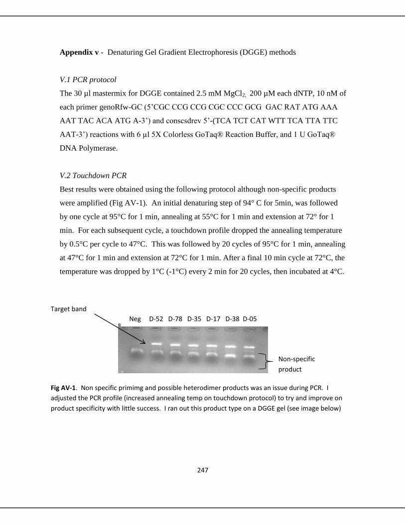
247
Appendix v - Denaturing Gel Gradient Electrophoresis (DGGE) methods
V.1 PCR protocol
The 30 µl mastermix for DGGE contained 2.5 mM MgCl2, 200 µM each dNTP, 10 nM of
each primer genoRfw-GC (5’CGC CCG CCG CGC CCC GCG GAC RAT ATG AAA
AAT TAC ACA ATG A-3’) and conscsdrev 5’-(TCA TCT CAT WTT TCA TTA TTC
AAT-3’) reactions with 6 µl 5X Colorless GoTaq® Reaction Buffer, and 1 U GoTaq®
DNA Polymerase.
V.2 Touchdown PCR
Best results were obtained using the following protocol although non-specific products
were amplified (Fig AV-1). An initial denaturing step of 94° C for 5min, was followed
by one cycle at 95°C for 1 min, annealing at 55°C for 1 min and extension at 72° for 1
min. For each subsequent cycle, a touchdown profile dropped the annealing temperature
by 0.5°C per cycle to 47°C. This was followed by 20 cycles of 95°C for 1 min, annealing
at 47°C for 1 min and extension at 72°C for 1 min. After a final 10 min cycle at 72°C, the
temperature was dropped by 1°C (-1°C) every 2 min for 20 cycles, then incubated at 4°C.
Fig AV-1. Non specific primimg and possible heterodimer products was an issue during PCR. I
adjusted the PCR profile (increased annealing temp on touchdown protocol) to try and improve on
product specificity with little success. I ran out this product type on a DGGE gel (see image below)
Target band
Neg D-52 D-78 D-35 D-17 D-38 D-05
Non-specific
product

248
V.3 Running the DGGE gel
DGGE was conducted following the same protocol of Muyzer et al. (1993) using an
Ingeny PhorU Electrophoresis System (Ingeny, Goes, Netherlands). DGGE gels
contained 6% (w/v) polyacrylamide denaturing gradient gels with linear gradients from
15% to 55% of denaturing agent (where 100% is 7M urea and 40% (v/v) formamide).
Base on product intensity on 1% agarose gel, 10-50 ng product was loaded onto the
DGGE gel and run in 1 x TAE at 100V, 200ma at 60°C for 16 hours. Gels were stained
with 1X SYBR-Gold (Invitrogen, Carlsbad) solution in 1X TAE buffer (Fig. Av-2)
Fig Av-2. Image of DGGE gel using product amplified using the described above.
Individual signatures were observed, but target fragments could not be isolated.
An effort was then made to clean up the product by excising the desired band on a low melt
agarose gel (Sigma). Unfortunately, product yields were too low to perform DGGE (Fig.
AV-3)
Fig. Av-3. Figure illustrates low post excision DNA yields
500 base
pairs
Ld D52 D78 D35 D17 D38 D05 D61 D78

249
Related Documents