Genetic algorithms for complex hybrid flexible flow line problems

Genetic algorithms for complex hybrid flexible flow

line problems

Thijs Urlings1∗, Rubén Ruiz1, Funda Sivrikaya Şerifoğlu2

1 Grupo de Sistemas de Optimización Aplicada, Instituto Tecnológico de Informática,

Universidad Politécnica de Valencia, Valencia, Spain.

[email protected],[email protected]

2 Abant Izzet Baysal University. Dept. of Management.

Bolu, Turkey. [email protected]

March 7, 2007

Abstract

This paper introduces some new genetic algorithms for a complex hybrid flexi-

ble flow line problem with the makespan objective. General precedence constraints

among jobs are taken into account, as are machine release dates, time lags and se-

quence dependent setup times; both anticipatory and non-anticipatory. This com-

bination of constraints implies a close connection to real-world industrial problems.

The introduced algorithms employ solution representation schemes with different

degrees of directness. Several new machine assignment rules are introduced and

implemented in the genetic algorithms, as well as in some existing heuristics. The

genetic algorithms are compared to these heuristics, to a MIP model and to a ran-

dom solution generator. The results indicate that simple solution representation

schemes result in the best performance.

Keywords: hybrid flexible flow line, realistic scheduling, precedence constraints,

setup times, time lags, genetic algorithms.

∗Corresponding author. Tel: +34 963 877 237. Fax: +34 963 877 239

1

1 Introduction

In this paper, we address a complex hybrid flexible flow line scheduling problem using a ge-

netic algorithm approach. Since the first studies on scheduling by Salveson [38] and Johnson

[16], a rich body of literature has appeared including a wide range of problems with various

characteristics. Yet, many researchers have noted in their papers that there has always been

a so-called gap between the theory and practice of scheduling (Allahverdi et al. [1], Dudek

et al. [8], Ford et al. [9], Ledbetter and Cox [19], Linn and Zhang [22], MacCarthy and Liu

[25], McKay et al. [26, 27], Olhager and Rapp [32], Vignier et al. [43]). Reisman et al. [34]

provide a statistical review on flowshop sequencing/scheduling research between years 1952-

1994. They discuss the exponentially growing body of literature on this subject and conclude

that from a total of 170 reviewed papers, only 5 (i.e. 3%) dealt with true applications.

According to Schutten [39], high level algorithms are developed in the operations research

literature, but side constraints that occur in practice are not considered. He tries to fill the

gap with production literature, in which myopic algorithms such as priority rules are used to

solve practical problems. The paper illustrates how the shifting bottleneck procedure for the

classical job shop can be extended to deal with practical features such as transportation times,

setups, downtimes, multiple resources and convergent job routings. Allaoui and Artiba [2] also

conjecture that there is a large gap between the literature of scheduling and the real life indus-

try. The paper deals with a practical and stochastic hybrid flow shop scheduling problem with

setup, cleaning and transportation times and maintenance constraints to optimize several ob-

jectives based on flow time and due dates. Another paper involving realistic considerations is

provided by Low [24] who considers a flowshop with multiple unrelated machines, independent

setup and dependent removal times. A simulated annealing (SA)-based heuristic is proposed

to optimize the total flow time in the system.

Although there is a recent trend towards more realistic formulations of scheduling problems

such as the ones reviewed above, there are still not many research efforts to jointly consider re-

alistic constraints prevailing in real-world manufacturing environments. One important draw-

back is that the solutions of such complex problems are rather difficult to obtain. Indeed,

heuristic and metaheuristic solution approaches are needed to obtain good solutions in rea-

sonable computational times. Yet, a wealth of such solution approaches may be developed

with different degrees of “blindness” to problem specific knowledge representing interesting

tradeoffs. This study aims to investigate such tradeoffs by making use of a genetic algorithm

approach to a complex hybrid flexible flowshop problem. Different representation schemes

with varying degrees of directness are employed, and the effects on solution quality and com-

2

putation times have been explored. The results are compared to the ones obtained by several

heuristics and by a MIP modelization of the same problem on an extensive set of benchmark

instances (Ruiz et al. [37]).

The rest of the paper is structured as follows: Section 2 gives a literature review on realistic

scheduling problems and genetic algorithm applications. The considered problem is described

in Section 3. Different machine assignment rules are introduced in Section 4. The proposed

methods are detailed in Section 5. Section 6 provides the computational and statistical eval-

uation of the results and of the comparison with other solution methods. Finally, conclusions

are given in Section 7.

2 Literature review

2.1 Genetic algorithm applications in realistic scheduling

Genetic algorithms (GAs) are a popular tool used for solving a range of optimization problems

including realistic scheduling problems. Oduguwa et al. [31] provide a survey on evolutionary

computation applications to real-world problems. The survey is on the applications of the

core methodologies of evolutionary computation. The results show that the majority of papers

reviewed employ variants of GAs.

Ruiz and Maroto [35] propose the adaptation of a genetic algorithm from an earlier study

to a more realistic problem with sequence dependent setup times, several production stages

with unrelated parallel machines at each stage, and machine eligibility. Such a problem is

common in the production of textiles and ceramic tiles. The proposed algorithm is tested

against several adaptations of other well-known metaheuristics to the problem using several

experiments with a set of random instances as well as with real data taken from companies of

the ceramic tile manufacturing sector.

An industrial application is given by Bertel and Billaut [3] on a three-stage hybrid flowshop

scheduling problem with recirculation. The problem is to perform jobs between a release date

and a due date, in order to minimize the weighted number of tardy jobs. An integer linear

programming formulation of the problem and a lower bound are proposed. A greedy algorithm

and a genetic algorithm are presented as approximate methods and evaluated on instances

like industrial ones. In another application, Tanev et al. [40] hybridize priority/dispatching

rules and GAs by incorporating several such rules in the chromosome representation of a GA

designed to solve a multiobjective, real-world, flexible job shop scheduling problem.

Lohl et al. [23] present an application of a genetic algorithm to a highly constrained real-world

scheduling problem in the polymer industry. The quality of the results and the numerical

3

performance is discussed in comparison with a mathematical programming algorithm. Dorn

et al. [7] describe an experimental comparison of four iterative improvement techniques for

schedule optimization including iterative deepening, random search, tabu search and genetic

algorithms. They apply these techniques on the data of a steel production plant in Austria.

Gilkinson et al. [13] present a GA application to solve the multi-objective real-world scheduling

problem of a company that produces laminated paper and foil products. The manufacturing

system is composed of workcell groups. Jobs may skip some stages. For certain products, it

is possible to process multiple jobs on a single machine.

2.2 Genetic algorithms for flexible flow line problems

GAs are also popular tools for the flexible flow line problems, although other approaches like

tabu search are also used, in this case for simpler problems (see for example Nowicki and

Smutnicki [30]). Leon and Ramamoorthy [21] explore problem-space-based neighborhoods for

industrial and randomly generated problems in the context of flexible flow line scheduling.

The search is conducted in neighborhoods generated by perturbing the problem data and not

solutions; hence the name. Three simple local search heuristics are proposed.

Kurz and Askin [17] schedule flexible flow lines with sequence dependent setup times to min-

imize makespan. An integer program is formulated and discussed. Because of the difficulty

in solving the integer program directly, several heuristics are developed, including a random

keys genetic algorithm which is found to be very effective for the problems examined.

More recently, Torabi et al. [41] investigate the lot and delivery scheduling problem in a simple

supply chain where a single supplier produces multiple components on a flexible flow line and

delivers them directly to an assembly facility. The objective is to minimize the average of

holding, setup, and transportation costs per unit time. They develop a mixed integer non-

linear program, an optimal enumeration method to solve the problem, and a hybrid genetic

algorithm which incorporates a neighborhood search.

2.3 Representation schemes for GA applications in scheduling

The choice of a representation scheme is an important decision in the design of a GA which

affects other design choices like the crossover and mutation operators, and eventually the per-

formance of the algorithm. In fact, an inappropriate representation may lead to the failure

of the algorithm itself. The representation schemes used in the GA approaches to schedul-

ing problems are various. Simple permutations of tasks (jobs, operations) are most popular.

Chromosomes representing priority values (Dhodhi et al. [6]), execution times (Nossal [29]),

and machine assignments (Woo et al. [45]) for tasks are also used. A compound representation

is provided by França et al. [10] for the problem of scheduling part families and jobs within

4

each part family in a flowshop manufacturing cell to minimize the makespan. The chromo-

some is a concatenation of strings. The first string gives the order, in which the families are

scheduled on different machines. The rest of the strings each give the order, in which the jobs

of a specific part family are processed.

The design decisions become more important for applications where the problem involves

precedence constraints. Usually, topological ordering of tasks is used in the chromosomes.

Ramachandra and Elmaghraby [33] try to minimize the weighted sum of the completion times

of a set of precedence-related jobs on two parallel identical machines. They test the results

obtained by a GA approach against that obtained by a binary integer programming model.

The chromosome representation is based on topological orderings of jobs, and schedules are

obtained by using the first available machine rule for machine assignments.

Kwok and Ahmad [18] schedule arbitrary task graphs onto multiprocessors, where the task

graphs represent parallel programs. The nodes of the graph are topologically ordered in the

chromosome, and they are assigned to the processors to minimize the overall execution time of

the program. Ge [11] addresses a similar problem, namely multiprocessor scheduling of graphs

representing data-flow programs. The researcher employes a systematic approach to generate

feasible permutations of nodes. The nodes (jobs) are grouped in clusters. In the chromosome

representation, nodes within the same cluster are sequenced randomly and clusters are con-

catenated deterministically.

Another compound type of representation scheme involves priority listings for tasks. Ca-

vory et al. [5] consider the cyclic job shop scheduling problem with linear precedence con-

straints. The chromosome representation of the GA approach is a compound of distinct sub-

chromosomes, each one related to a machine. Each sub-chromosome indicates a preference list,

corresponding to an order of priority for the processing of the tasks on the associate machine.

Gonçalves et al. [14] present a hybrid genetic algorithm for a job shop scheduling problem.

The chromosome representation of the problem is based on random keys. It includes 2n genes

where n is the number of operations. The first n genes give operation priorities. The second set

includes factors to be used in the computation of delay times for the operations. Ghedjati [12]

also uses priority information in the chromosome structure, this time in a two-dimensional

representation scheme. She addresses job-shop scheduling problems with several unrelated

parallel machines and precedence constraints between the operations of the jobs (with either

linear or non-linear process routings). A chromosome consists of two parts. The first part

contains indices of priority rules to be used for operation assignment, the second part indices

corresponding to one of the seven heuristics for machine assignment. Similarly, Wang et al. [44]

also use a chromosome structure consisting of two parts in their application to the matching

and scheduling of interdependent subtasks of an application task in a heterogenous computing

environment. The matching string represents the subtask-to-machine assignments, and the

5

scheduling string gives the execution ordering of the subtasks assigned to the same machine.

Representation schemes other than task orderings and priority listings are also used although

not as often. Nossal [29], for example, presents a genetic algorithm for multiprocessor schedul-

ing of dependent, periodic tasks. The scheduling problem is encoded by deriving execution

intervals for the tasks, which determine the temporal boundaries for the execution points in

time. The genetic algorithm selects the actual start time for each task from within the corre-

sponding interval. The scheduler builds and then assesses the associated schedule with regard

to the fulfillment of the deadlines of the tasks and the inter-task relations.

3 Problem description

We now proceed with the definition of the complex problem we deal with in this paper.

The hybrid flexible flow line problem (HFFL) can be described as follows: Given is a set

of jobs N = {1, . . . , n} to be processed on a production line, consisting of a set of stages

M = {1, . . . ,m}. Each stage i, i ∈ M contains a set of unrelated machines Mi = {1, . . . ,mi}.

The flexibility of the problem implicates that jobs might skip stages. Each job j, j ∈ N visits

a set of stages Fj ⊆ M (Fj 6= ∅). The processing time for job j on machine l at stage i is

denoted pilj . These times depend on the job and the machine, as machines are unrelated, and

are zero for all the machines at stages that the job does not visit (pilj = 0,∀i /∈ Fj).

For this hybrid flexible flow line we consider the following constraints, also treated in Ruiz

et al. [37].

• Eij ⊆ Mi is the set of eligible machines for job j in stage i. This means that not all

machines at a given stage might process job j. Consider for example a stage with a small

and a large machine. Small products can be processed on either of the two machines

whereas large products can only be processed on the large one. Note that pilj = 0 if

l /∈ Eij. Also Eij 6= ∅ if i ∈ Fj .

• rmil expresses the release date for machine l in stage i. No operation can be started at

machine l before rmil. This allows us to model machines that did not finish previous

work yet.

• Pj ⊂ N gives set of predecessors of job j. Job j cannot start until all jobs in Pj have

finished. This is the case if auxiliary products are needed to start the processing of the

final product.

• lagilj models the time lag for job j between stage i and the next stage to be visited,

when job j is processed on machine l at stage i. A job in reality often consists of a

large quantity of products with the same specifications. If so, the first products can in

6

many cases be processed at the next stage before finishing the whole job. In other cases,

the start at a next stage might be delayed because of products that have to dry or cool

down. Negative time lags model the former cases whereas positive time lags model the

latter ones. In case of negative time lags, |lagilj | is never greater than pilj, nor than any

of the processing times in the next visited stage.

• Siljk denotes the setup time between the processing of job j and job k on machine l inside

stage i. We treat sequence dependent setup times, as the setup time between painting a

black product and a white one might be larger than the time needed if the white product

is processed before the black one. These setup times are assumed separable from the

processing time.

• Ailjk is a binary parameter that indicates whether the corresponding setup is anticipa-

tory (1) or not (0). Most machine setups can be performed before the product enters

the stage, but in some cases (to attach the product to the machine, for example) setup

has to be postponed until the product arrives at the machine.

In real production situations a frequent goal is to finish a certain client order as early as

possible. Our objective is therefore to minimize the maximum completion time, which is

well known in the literature as makespan. If we denote by Cij the completion time of job j

at stage i and LSj = maxi∈Fj

i the last stage visited by job j, we can define the makespan as

Cmax = maxj∈N

CLSj ,j. Using the three field notation by Vignier et al. [43] we can define this

HFFL problem as: HFFLm, ((RM (i))(m)i=1)/Mj , rm, prec, Sijk, lag/Cmax.

Although the number of feasible solutions is reduced by machine eligibility, stage skipping

and precedence constraints, many simplifications of this problem have been proven to be NP-

Hard. Actually the standard hybrid flow shop problem is just a special case of this HFFL

problem. Lee and Vairaktarakis [20] showed NP-hardness of hybrid flow shop problems in

general. That precedence relationships do not simplify the problem can be concluded by Ull-

man [42], who proved that the two parallel machine problem with precedence constraints is

already NP-Hard. The same holds for setup times, as Gupta [15] classified the regular flow

shop with sequence dependent setup times as NP-Hard.

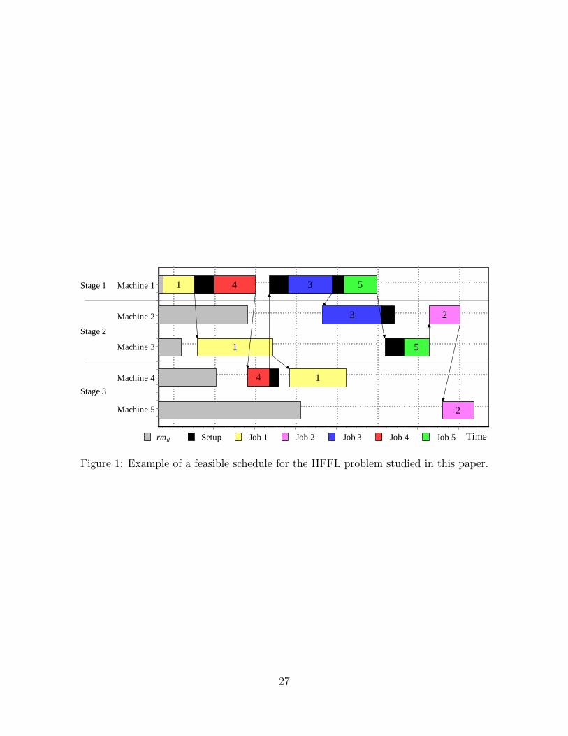
In Figure 1, an example of a solution of the considered hybrid flexible flow line scheduling

problem is shown. This instance consists of 5 jobs, 3 stages and 5 machines and includes stage

skipping, machine release dates, both anticipatory (between job 4 and job 1 on machine 4) and

non-anticipatory (between job 4 and job 3 on machine 1) setups, positive (job 1) and negative

(job 4) time lags, and precedence relationships (between job 4 and job 3).

[Insert Figure 1 about here]

7

4 Machine assignment rules

As has been shown earlier, there are many possible solution presentations for the HFFL prob-

lem. Representations as simple as job permutations are possible, as well as complex job-

machine multiple arrays or even chromosomes with starting times. For the HFFL problem

with Cmax objective, however, a non-delay schedule includes the optimum solution so there is

no need to include starting times in the solution encoding. The solution space is much smaller

with a permutation representation. However, only a simple job permutation does not suffice.

Given a certain job permutation, jobs have to be assigned to an eligible machine at each stage.

Therefore, we implemented some existing and some new machine assignment rules.

Given a certain job permutation, decisions have to be taken on the machine assignments at

each stage. For those decisions nine machine assignment rules have been developed. One of the

rules is applied to all the stages a job visits before starting the assignments of the next job in

the permutation. All rules calculate a value for each eligible machine using static information

on the problem instance and dynamic information on the partial schedule established so far.

The machine with the minimal value is chosen.

To describe the machine assignment rules some additional notation needs to be defined. The

machine assigned to job j at stage i is denoted by Tij or by l in brief. The previous job that

was processed at machine l is denoted by k(l). Let stage i − 1 be the last stage visited by

job j before stage i, stage i + 1 the next stage to be visited, and stages FSj and LSj the

first and last stages job j visits, respectively. Let furthermore Ai,l,k(l),j = Si,l,k(l),j = 0 for

i /∈ Fj or i ∈ Fj but l /∈ Eij and Ai,l,k(l),j = Si,l,k(l),j = Ci,k(l) = 0 when no preceding job

k(l) exists. Completion times for job j at all visited stages can now be calculated with the

following expressions:

CFSj,j = max{rmFSj ,l;maxp∈Pj

CLSp,p;CFSj ,k(l) + AFSj ,l,k(l),j · SFSj ,l,k(l),j}

+(1 − AFSj ,l,k(l),j) · SFSj,l,k(l),j + pFSj ,l,j, j ∈ N(1)

Cij = max{rmil;Ci,k(l) + Ai,l,k(l),j · Si,l,k(l),j;Ci−1,j + lagi−1,Ti−1,j ,j}

+(1 − Ai,l,k(l),j) · Si,l,k(l),j + pilj , j ∈ N, i > FSj

(2)

The calculations should be made job-by-job to obtain the completion times of all tasks. For

each job, the completion time for the first stage is calculated with Equation (1), considering

availability of the machine, completion times of the predecessors, setup and its own processing

time. For the other stages Equation (2) is applied, considering availability of the machine,

availability of the job (including lag), setup and its processing time.

If job j is assigned to machine l inside stage i, the time at which machine l completes job j

is denoted as Lilj. Following our notation, Lilj = Cij given Tij = l. Furthermore, we refer

8

to the job visiting stage i after job j as job q and to an eligible machine at the next stage as

l′ ∈ Ei+1,j.

Suppose now that we are scheduling job j in stage i, i ∈ Fj . We have to consider all machines

l ∈ Eij for assignment. The proposed assignment rules are the following:

1. First Available Machine (FAM): Assigns the job to the first eligible machine available.

This is the machine with the minimum liberation time from its last scheduled job, or

lowest release date if no job is scheduled at the machine yet, i.e. Tij = l such that

minl∈Eij

Lilk.

2. Earliest Starting Time (EST): Chooses the machine that is able to start job j at the

earliest time. Therefore we also have to take the availability of the job and setup times

into account. Assigns to the machine l with minl∈Eij

{Lilj − pilj}, as the starting time can

be represented as the finish time minus the processing time.

3. Earliest Completion Time (ECT): Takes the eligible machine capable of completing job

j at the earliest possible time. Thus the difference with the previous rule is that this

rule includes processing times. Job j is assigned to machine l such that minl∈Eij

Lilj.

4. Earliest Preparation Next Stage (EPNS): The machine able to prepare the job at the

earliest time for the next stage to be visited is chosen. Therefore time lags between the

current and the next stage are taken into account by assigning job j to machine l with

minl∈Eij

{Lilj + lagilj}. The rule uses more information about the continuation of the job,

without directly focusing on the machines in the next stage. If i = LSj this rule reduces

to ECT.

5. Earliest Completion Next Stage (ECNS): The availability of machines in the next stage

to be visited and the corresponding processing times are considered as well. Note that

we are assigning only to stage i. Then machine l with minl∈Eij ,l′∈Ei+1,j

{Li+1,l′,j|Tij = l} is

assigned to job j. The rule reduces to ECT if no single minimum is found, or if i = LSj.

6. Forbidden Machine (FM): Excludes machine l∗ that is able to finish job q earliest. ECT

is applied to the remaining eligible machines for job j. While the foregoing rules are

greedy, worse results might be expected for later jobs. This rule is supposed to obtain

better results for later jobs, as it reserves the machine able to finish the next job earliest.

Mathematically, we choose machine l considering minl∈Eij

{Lilj − |l − l∗| · I} where I is a

high positive number and l∗ given by minl∗∈Eiq

{Li,l∗,f + Si,l∗,f,q + pi,l∗,q}, job f being the

last job scheduled at l∗. Note that job j is assigned to machine l∗ if this is the only

9

eligible machine. ECT is applied if j ∈ Pq as job j has to be finished as early as possible

in this case, or if job j is the last job at stage i.

7. Next Job Same Machine (NJSM): The assumption is made that job q is assigned to

the same machine as job j. Assigned machine Tij is chosen such that job q is finished

earliest. So machine l is chosen by optimizing minl∈Eij

Lilj +Siljq + pilq. Note that only job

j is assigned. The rule is especially useful if setups are relatively large, as the foregoing

rules do not take the setup between job j and job q into account. Reduces to ECT if

job j is the last at this stage.

8. Sum Completion Times (SCT): Completion times of job j and job q are calculated for

all eligible machine combinations Eij × Eiq at stage i. Machine l is chosen such that

the sum of both completion times is the smallest: minl∈Eij ,l∗∈Eiq

{Lilj + Li,l∗,q}. Similar to

NJSM, but without the assumption that job q is assigned to the same machine. Reduces

to ECT if job j is the last at stage i.

9. Anticipatory Based (AB): Concentrates on possibilities for future anticipatory setups.

Non-anticipatory setups might cause important delays. Therefore this rule tries to

avoid this type of setups. Anticipation factor AFl =∑

h∈H

Ailjh · Siljh/|Eih| expresses

the expected advantage caused by the anticipatory setups, H being the set of jobs

sequenced after job j. The factor is subtracted from the EPNS value and the result

minl∈Eij

{Lilj + lagilj −AFl} gives the machine l to which to assign job j. Reduces to EPNS

if job j is the last job at this stage.

Especially for the first five assignment rules, the growing amount of information used rep-

resents a tradeoff between the probability on good schedules on the one hand, and valuable

computation time on the other hand. The remaining four rules are designed for alternative

assignments, concentrating on drawbacks of the earlier rules.

5 Heuristics and genetic algorithms

5.1 Heuristic methods

With this variety of assignment rules we can easily improve the existing heuristics. In Ruiz

et al. [37] several dispatching rules and an adaptation of the heuristic by Nawaz et al. [28]

(NEH) were proposed for this hybrid flexible flow line. The implemented dispatching rules

are Shortest Processing Time (SPT), Longest Processing Time (LPT), Least Work Remaining

(LWR), Most Work Remaining (MWR) and Most Work Remaining with Average Setup Times

10

(MWR-AST). As all these methods require small CPU times, we can simply apply for each

heuristic all nine machine assignment rules. As a result, we pick for each heuristic the best

solution out of the nine we obtained. For more details about the heuristics the reader is

referred to Ruiz et al. [37].

5.2 Genetic Algorithms

We have implemented five genetic algorithms with different solution encodings, representing a

tradeoff: A too verbose representation results in an inefficient algorithm due to the large search

space and a too compact representation might exclude important solutions in the process.

The makespan of individual x, Cmax(x) determines the solution value of x. Three different

selection types are implemented for the GAs. Random selection is straightforward. Tourna-

ment selection directly uses the makespan value. Five individuals are randomly selected for

a tournament. The individual with the lowest makespan is subjected to crossover with an-

other individual selected similarly. Roulette selection assigns to each individual a fitness value

Fx = maxy∈Pop

Cmax(y) − Cmax(x) + 1. An individual x is chosen with probability Fx/∑

y Fy.

Pop is the population of solutions in the GA.

5.2.1 Basic Genetic Algorithm: BGA

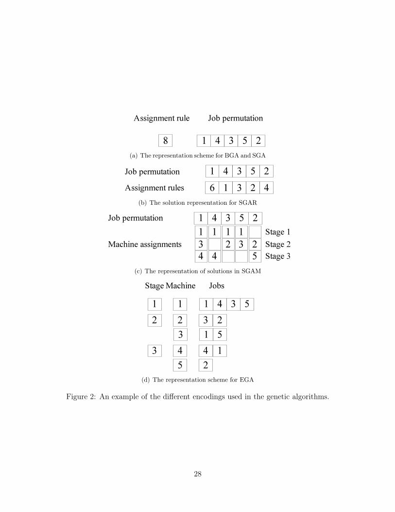
The solution representation of the basic genetic algorithm (BGA) is most compact, consisting

of a job sequence and the machine assignment rule used for all jobs. The chromosome size is

n + 1, as can be seen in Figure 2(a). Note that not all possible solutions are reachable with

this representation. For example, the solution given in Figure 1 is not reachable since the jobs

do not visit the machines in the same order (non-permutation solutions).

The implemented crossover operators are One-Point Order Crossover (OP), Two-Point Order

Crossover (TP) and Uniform Order Crossover (UOX). All maintain feasibility with respect to

the precedence constraints.

Mutation is applied probabilistically to each job. Position Mutation (PM) interchanges the

job with another randomly selected job and Shift Mutation (SM) places the job into another

randomly selected position. PM and SM are adapted for precedence constraints, i.e., we use

precedence-safe PM and SM operators: Within both mutations, the minimum and maximum

allowed position in the current sequence are determined for the associate job. The new posi-

tion is chosen randomly within this range.

Mutation is also applied to the assignment rule: The rule is simply replaced by another ran-

domly chosen one. All these operators (crossover, job mutation and machine assignment rule

mutation) are applied with given probabilities.

The initial population is generated in the following way: for each machine assignment rule one

11

individual is generated by the NEH heuristic with applying the according machine assignment

rule. 75% of the individuals are generated by randomly sequencing eligible jobs; those jobs

whose predecessors have already been sequenced. The rest of the individuals are mutated

NEH solutions. After the generation of job sequences, a machine assignment rule is assigned

to each individual, to complete the population initialization.

The overall structure of the basic algorithm is as follows: The two best individuals of each

population are inserted into the new population (elitism approach). The rest of the new pop-

ulation is filled by individuals selected from the old population and subjected to crossover and

mutation.

[Insert Figure 2 about here]

5.2.2 Steady-State Genetic Algorithm: SGA

The second proposed algorithm (SGA) has a steady-state structure: New individuals substitute

the worst individuals of the current population as they are generated, but only if their solution

values are better than the worst values of the population and if the solution did not yet exist

in the population. As the best individuals of a population are never replaced, no elitism is

needed to maintain the best solutions. This approach has been applied with success in Ruiz

and Maroto [35] and in Ruiz et al. [36]. Note that only comparing the job sequence is not

enough to check uniqueness, because of the different machine assignment rules. We therefore

compare the makespan and if equal, we check the job sequence. The solution representation

and the operators remains the same as in BGA.

5.2.3 Steady-State GA with changing Assignment Rule: SGAR

Allowing independent machine assignment rules for every job in the sequence yields our next

algorithm (SGAR). This changes the solution representation as shown in Figure 2(b). Apart

from the job sequence, an assignment rule for each job is stored in a second array of size n,

which increases the chromosome size to 2n. This algorithm uses the steady state structure

and all operators defined before in the BGA algorithm. In the crossover, the assignment rule

of each job is copied along with the jobs from the parents. When mutation is applied, rules

stick with the associated jobs. The assignment rule of each job is subjected to mutation in

the assignment rule mutation phase.

12

5.2.4 Steady-State GA with Machine Assignments: SGAM

A more verbose solution representation contains, for each stage, the machine assigned to each

job. This means that there is, apart from the job sequence, an m×n matrix with the machine

assignments for each job and stage. These exact machine assignments replace the machine

assignment rules in the chromosome. The chromosome of size (1 + m)n for this algorithm

is demonstrated in Figure 2(c). The proposed algorithm (SGAM) also uses the steady state

structure and all previously explained operators. During crossover, assignments for a given job

are taken over from the parent that passes the job, as in SGAR. Assignment mutation changes

a single random machine assignment for each job. Furthermore, a second machine assignment

mutation compares the current makespan with the makespan of the schedule resulting from

implementation of a random assignment rule. If the assignment rule improves the makespan,

all machine assignments in the original individual are replaced by the assignments in the

solution that results from the assignment rule. This helps the algorithm to encounter good

machine assignments earlier.

5.2.5 Steady-State GA with Exact Representation: EGA

With the exact representation, used in algorithm EGA, also non-permutation solutions are

reachable. This is interesting, as the optimal schedule might be a non-permutation one (see

for example Figure 1). For the makespan objective, one can represent any feasible solution,

given the tasks processed at each machine in the order the machine will process them (see

Figure 2(d)). There is no reason to delay any tasks, so all tasks are started at the earliest

possible moment, given by Equations (1) and (2) in Section 4. The size of this representation

is equal to the number of tasks, which is equal to∑

j∈N |Fj |.

Most operators defined for the other representations cannot be used anymore. For crossover,

two operators are proposed. Guaranteed Feasibility Crossover (GFX) maintains a list of all

available tasks for the assignment to the offspring: tasks whose start times can directly be

derived. Among the tasks that are not scheduled yet, the ones that are available and not

preceded by other unscheduled tasks in their machine, are stored in a list for this parent.

At each iteration, either one of the two parents is chosen and a random task from this list

is assigned to the same machine in the child’s chromosome. When a complete schedule is

obtained for the first child, the process is repeated for the second child. An example: Suppose

parent 1 represents the solution in Figure 1 and parent 2 is an arbitrary other individual. At

the start (iteration 1) the tasks of job 1, job 4 and job 5 in stage 1 are available. Suppose the

toss is won by parent 1. Only job 1 at stage 1 is a candidate, and therefore scheduled as the

first job at machine 1 for the offspring. At iteration 2, Job 4 and job 5 are available in stage 1

and job 1 in stage 2. Suppose the toss is won again by parent 1. Job 4 at machine 1 and job 1

13

at machine 3 are the candidates. Suppose job 4 at machine 1 is chosen. Then job 5 at stage 1,

job 1 at stage 2 and job 4 at stage 3 are available for iteration 3. This procedure is continued

until no tasks are available any more; all tasks are scheduled and the offspring is completed.

Fast Crossover (FX) is similar to GFX, but no list of available tasks is maintained. For both

parents only a list is maintained with the first unscheduled task in each machine. One of these

tasks is scheduled at the same machine for the child. Note that feasibility of the offspring is

not guaranteed. In contrast, FX crossover is much faster than GFX.

Similarly, two mutations can be applied to the machine assignment arrays in the chromosomes.

Both place a task at a new position in any of the eligible machines in the same stage. Fast

Mutation (FM) checks the precedence relationships within the new machine. The new position

is chosen randomly between the minimum and maximum position, according to the direct

precedence relations. This, however does not guarantee global feasibility. We use Figure 1 as

an example. If we apply mutation on job 2 in stage 3, direct precedence constraints do not

impose any position in machine 4 or 5. The only predecessor is job 5, which does not visit

stage 3. However, placing this task before job 4 in machine 4 leads to an infeasible solution.

In this solution, job 4 cannot be finished before termination of job 2. Therefore, (and because

of the precedence relation between job 3 and 4) job 3 cannot be started before termination of

job 2. But because of the orden in machine 2, job 2 cannot be started before termination of

job 3 in this machine.

Guaranteed Feasibility Mutation (GFM) assures that the new schedule is feasible. In case of

precedence constraints this implies not only direct predecessors and successors, but also needs

a recursive search for their anterior and posterior jobs in other stages respectively. Obviously

this implies a larger cost in running time, but no solutions have to be discarded.

A new individual only substitutes the worst individual if the chromosome has been changed

by crossover or mutation, if it is feasible and if it has a solution value lower than the value of

the worst individual.

The NEH method is not directly applicable for this representation, but we can transfer the

NEH solutions made with the less complex representation. Population initialization therefore

does not change.

5.3 Random Scheduling

Boyer and Hura [4] implemented a random scheduling (RS) algorithm for sequencing all tasks

in a distributed heterogeneous computing environment. They show that their algorithm is

less complex than evolutionary algorithms, computes schedules in less time and requires less

memory and fewer parameter fine-tuning. We therefore implement an RS algorithm, which

produces new individuals without crossing or mutating them. The individuals are represented

14

by a random feasible job sequence and a machine assignment rule (see Figure 2(a)).

6 Experimental evaluation

To test, compare and analyze the algorithms we use a subset of the benchmark proposed

by Ruiz et al. [37]. The benchmark contains two data sets for the problem, including 10

factors designed with a large number of levels. Ruiz et al. [37] show that various levels for

the controlled factors do not have a significant influence on the hardness of the instances.

Therefore we eliminate these levels from the experiments. The levels we use for the first data

set are given in Table 1. The second set contains larger instances. The modified levels for this

set are shown in Table 2.

For each level, there are three instances, resulting in a total of 768 instances; 576 small and

192 large instances. For instances with only one machine per stage, the machine assignments

are trivial. We therefore distinguish the set of instances with mi = 1 from the set with mi = 3

in the small set.

[Insert Tables 1 and 2 about here]

The stopping criterion for all genetic algorithms and RS method is given by a time limit

depending on the size of the instance. The algorithms are stopped after a CPU running

time of n∑

i mi · t milliseconds, where t is an input parameter. Giving more time to larger

instances is a natural way of decoupling the results from the lurking “total CPU time” variable.

Otherwise, if worse results are obtained for large instances, it would not be possible to tell if

it is because of the limited CPU time or the instance size.

6.1 Calibration

Before calibration, the algorithms are subjected to some preliminary tests to reduce the number

of levels of the parameters to be tested in the fine-tuning process. Shift Mutation performed

clearly better than Position Mutation in preliminary experiments, allowing us to keep the lat-

ter out of further consideration. As TP is not outperformed by the other crossover operators

for any GA, this operator chosen for BGA, SGA, SGAR and SGAM. The Fast Crossover for

EGA yields worse results than GFX; it does not even yield any feasible children at all for

large instances with precedence constraints. Therefore, comparison of crossovers for EGA is

not needed either, and GFX is chosen.

A range of tests for the machine assignment rules shows that ECT, EPNS, ECNS and NJSM

yield better results on average than the other remaining rules, although the other rules give

better results in some occasions. Therefore, only these four rules are used for mi > 1; for

15

mi = 1 no rule has to be applied. The corresponding four NEH solutions seeding the initial

GA populations are generated for instances with mi > 1; for mi = 1, the standard NEH

method is used to obtain one solution. The probability of the bit mutation changing the

machine assignment rule is 0 for mi = 1 and otherwise fixed at 5% per individual for BGA

and SGA and at 1% for SGAM; 1% per job for SGAR. Recall that in SGAM the machine

assignment rule is only used to compare between the current makespan and the makespan

obtained by applying this rule on the same job sequence. Comparison will be done with a

probability of 1% for each new individual.

For all GAs, crossover probabilities (Pc) of 40% and 60% are tested. Job mutation probabil-

ities (Pmut) are either 1% or 2% per job for BGA, SGA, SGAR and SGAM and either 1%

or 5% per machine for EGA. As commented, the four best assignment rules are used. To

test the necessity of various machine assignment rules, a level is added where only EPNS is

applied, which implies that the assignment rule mutation probability is 0. For all algorithms,

population sizes of 50, 80 and 200 are compared as are all three selection methods. Note that

RS is not calibrated as it does not have any parameters. The machine assignment rule in RS

is randomly chosen among ECT, EPNS, ECNS and NJSM.

The aforementioned setting results in a total number of parameter levels of 72. Each algorithm

is tested five independent times on each given parameter setting and instance. As for t in the

stopping time formula, we test t = 5 and 25 milliseconds. We used a Pentium IV computer

with 3.0 GHz processor and 1 GB of RAM memory for all tests.

By means of a multi-factor ANOVA - an analysis of variance for multiple factors - we compare

the various levels of the parameters. Because of the high quantity of results, the three ANOVA

hypotheses of normality, homoscedasticity and independence of residuals are easily fulfilled. In

all comparisons, we use confidence intervals of 99.9%, which means that we falsely accept an

hypothesis with a probability of only 0.1%. The dependent variable is the relative deviation

from the best known solution value, as the optimum is often not known.

Considering the algorithm parameters, the instance characteristics and the time limit, the

algorithm parameters appear least important. This indicates that the algorithms are robust

and do not depend on the instance parameters nor on the time limit. For the sake of brevity,

we do not go into detail on the analysis of the instance characteristics and limit ourselves to

the parameter calibration.

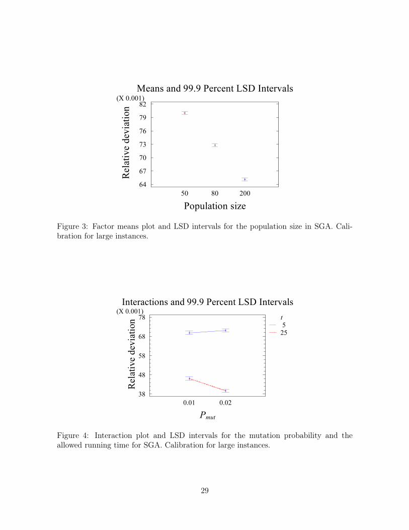
We will explain the calibration of SGA for the set of large instances in detail. The results

of the calibration of other algorithms and instance sets are obtained by applying the same

procedure. The algorithm parameter with the highest F-ratio is the population size, with

a value of 2799. This value is much higher than the F-value of the interaction with time

16

parameter t (about 15), which indicates robustness and makes a separated analysis of the factor

unnecessary. Investigation of the factor means plot (see Figure 3) shows that a population

size of 200 is most suitable. Note that non-overlapping intervals give a 99.9% guarantee

of a statistically significant difference in the observed means for the factor’s levels. To avoid

unexpected behaviour, we do not choose population sizes higher than 200 and fix the parameter

at this value. Running a new ANOVA for the remaining factors with the fixed population

size, the selection method appears to be the most influencing factor with an F-ratio of 1256;

again higher than the interaction F-ratio. We fix selection at the most advantageous method:

random selection. The steady-state structure of the algorithm implies a more exploitative

pressure than the generational structure of BGA, which asks for a smaller pressure in the

selection. The next ANOVA indicates that the mutation probability factor is most important

with an F-ratio of 49. The interaction with the time, however, is more important. Figure 4

shows this interaction. As a 2% probability is better for t = 25 and no significant difference

is observed for t = 5, we fix the probability at 2%. Of the remaining factors, only crossover

probability is significant (without interaction) and therefore fixed at 60%. Either usage of the

four machine assignment rules, or only applying EPNS stays unfixed for the moment due to

experiments being inconclusive. After calibration of all GAs for all instance sets, we fix the

insignificant parameters at the most convenient levels.

The final parameters for all GAs for all instance sets are listed in Table 3. Note that SGAR

and SGAM are not calibrated for instances with a single machine per stage, as the algorithms

only differ from SGA in machine assignment decisions. Machine assignments are trivial for

these instances. We can conclude that the proposed genetic algorithms are robust as regards

CPU time stopping criterion and instances’ characteristics.

6.2 Comparison between GAs

The calibrated algorithms are tested with t = 125 milliseconds for the CPU time limit. We

first compare the solution quality of the various calibrated genetic algorithms among them-

selves. An ANOVA for the smallest instances (mi = 1) shows that stage skipping PFj is the

most important factor over the algorithms, all the instance properties and running time. Stage

skipping makes the problem easier, as less tasks are involved. There is no interaction with

the algorithms however, which form the second most important factor. Although the exact

solution used in EGA is complete (i.e., the optimum solution is reachable), this algorithm is

on average worse than BGA and SGA, which in turn do no differ significantly for a confidence

interval of 99.9%.

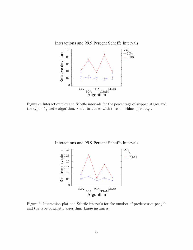
For mi = 3 the percentage of eligible machines PEij is the most important factor. The per-

centage of eligible machines logically influences the importance of machine assignments. The

17

interaction between the algorithm and PEij is shown in Figure 5. Note that Scheffe intervals

are used, which are more reliable for 10 factor levels (they counteract the bias in multiple

pairwise comparisons). If only half of the machines is eligible the differences are small, but

if all machines can process all jobs, the machine assignment rules are proven to be more ef-

ficient than incorporating the assignments in the representation. This is a counter-intuitive

result since one should expect an exact machine assignment representation to perform better.

However, the proposed machine assignment rules outperform the exact representations.

For the large instances the most important factor is NPj , i.e., the number of predecessors.

These constraints make the problem harder to solve for the GAs. The interaction of this factor

and the GAs can be found in Figure 6. Again, we find here another counter-intuitive results.

Presumably, with precedence constraints, less job permutations are feasible and therefore the

search space becomes smaller. However, the operators of the GAs are much more time consum-

ing when precedence relations are present in order to preserve feasibility and hence the worse

results. One can observe that the influence difference is especially large for EGA and SGAM.

The complicated EGA operators are especially slow under precedence constraints and SGAM

spends more running time on machine assignments and has therefore less time to concentrate

on the job sequence, which is more important in the case of precedence constraints.

[Insert Figures 5 and 6 about here]

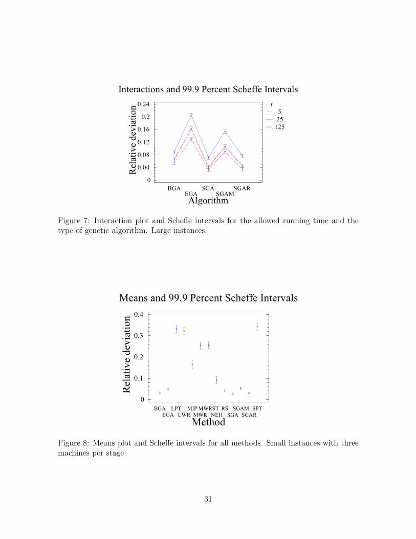
Also interesting is the performance of each algorithm for the different allowed running times,

shown in Figure 7 for the large instances. For EGA we see the behavior one would expect;

increasing the allowed running time leads to significantly better results. The same holds, in a

weaker sense, for SGAM. There is a clear improvement when increasing t from 5ms to 25ms,

but increasing further does not pay off. BGA, SGA and SGAR do obtain better solutions

with longer running times, but the difference is quite small. This proves that the algorithms

with less direct solution representations and therefore smaller search spaces, need less time to

explore a large part of the solution space than algorithms based on more verbose representa-

tions.

[Insert Figure 7 about here]

6.3 Comparison of all methods

To test the quality of the proposed GAs, we compare them with several other methods. For

small instances, the MIP results in Ruiz et al. [37] are used. For both small and larger in-

stances, we use the results of the dispatching rules and the specific adaptation of the NEH

18

heuristic, as described at the start of Section 5.

In Figure 8 the results for the small instances with three machines per stage are plotted for all

implemented methods. Note that the Scheffe intervals for all GAs and RS are narrower than

those of the MIP and heuristics methods. The reason is that for each instance, there is only

one result for the MIP and heuristics, as these are deterministic methods. For the GAs and

RS there are 15 results (five replicates and three t values). Note furthermore that we used

the MIP results with the time limit of 15 minutes (the best results obtained in Ruiz et al.

[37]). Some instances were solved to optimality within this time limit, some ended up with a

non-optimal solution and in a few cases no feasible solution was found within the 15 minutes

bound. The shown relative deviation is the average for all cases where a feasible solution was

obtained. The hardest instances are therefore not included in the average MIP deviation. It

is clear that the dispatching rules, although improved with the variety of machine assignment

rules, do not even approach the performance of any other method. However, one has to take

into account that the computation time for the dispatching rules is extremely short (for these

instances, less than a millisecond on average).

An even more important result is that all remaining methods give better results than the MIP

in less computation time. Not only the needed computation time is problematic for the model;

with longer running times the memory capacity becomes a problem, too.

NEH does not reach the solution quality of the GAs and RS, but we have to take into account

that this is a fast heuristic, compared to algorithms with longer running times.

Surprisingly, the performance of RS does not differ significantly from EGA’s and is even bet-

ter than the performance of SGAM. Apparently these two do not profit of the more verbose

solution representations; at least not for the tested running times. The simplicity and speed

of RS seems to be an advantage for solving a complex problem as the one addressed in this

article.

BGA, SGA and SGAR are the best implemented methods. The steady state structure seems to

be advantageous, but the difference is not significant. Introducing for each job an assignment

rule does not consume too much running time, but machine assignments are not improved

much either.

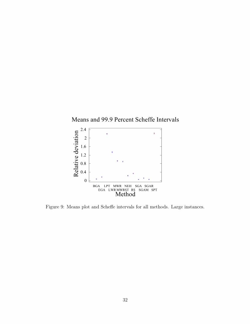
The results for the small instances with a single machine per stage (not shown) are similar.

Only SGAR and SGAM are left out since no machine assignment is needed in this case. Con-

centrating on the large instances (see Figure 9) some slight changes in the ranking are noticed.

The lack of structure in the solution search of RS starts to play a role when the search space is

larger. This method is therefore outperformed by NEH, which only needs about a second for

these instances. As already mentioned in the GA comparison, the operators in EGA are more

time consuming and this algorithm therefore results not very adapt for the large instances; it

19

finishes as the worst GA.

[Insert Figures 8 and 9 about here]

7 Conclusions and future work

In this paper, we have introduced various solution representations for a complex hybrid flexible

flow line problem. The addressed problem is more complex than the problems usually treated

in literature and allows for direct implementation in real-world situations.

The solution representations range from simple job sequences with a machine assignment rule

(BGA and SGA), job sequences with per-job machine assignment rules (SGAR), exact ma-

chine assignments (SGAM) to the exact representation of the solution with per-machine job

sequences (EGA). These representations are the basis of five genetic algorithms that are able

to solve larger instances than exact methods can and to obtain better results than heuristics.

Two new crossover operators and two new mutation operators are introduced for EGA and

for the other algorithms several new machine assignment rules are proposed, which we also

implemented in some existing heuristics.

For the evaluation and comparison of the different algorithms, a subset of an existing bench-

mark is used. All five genetic algorithms are subject to an elaborate parameter calibration,

using ANOVA statistical techniques. The algorithms prove to be robust with respect to the

allowed running time and to the characteristics of the instances.

Once calibrated, the genetic algorithms are compared to some other existing methods. For the

small instances the solution values of a MIP model with 15 minutes time limit are available.

For both the small and the large instances, five dispatching rules and a NEH adaptation, all

using the machine assignment rules, are used for comparison.

All genetic algorithms outperform the MIP model and all heuristics. A random solution gener-

ator (RS) with the same time limit as for the GAs is used for comparison. For small instances

RS is comparable to EGA and better than SGAM; for large instances all GAs show a better

performance.

The algorithms with less direct solution representations (BGA, SGA, SGAR) already show

good results for small allowed running time. More running time causes an insignificantly small

improvement in the solution value. The algorithms with more verbose solution representation

(SGAM and especially EGA) profit more from the extra time, but still do not reach the

solution quality of the earlier mentioned algorithms. We are therefore currently working

20

on an algorithm that combines several of the algorithms, starting with the most indirect

representation, changing towards more exact solution schemes.

References

[1] Allahverdi, A., Gupta, J. N. D., and Aldowaisan, T. (1999). A review of scheduling re-

search involving setup considerations. Omega-International Journal of Management Science,

27(2):219–239.

[2] Allaoui, H. and Artiba, A. (2004). Integrating simulation and optimization to schedule

a hybrid flow shop with maintenance constraints. Computers and Industrial Engineering,

47(4):431–450.

[3] Bertel, S. and Billaut, J. C. (2004). A genetic algorithm for an industrial multiprocessor

flow shop scheduling problem with recirculation. European Journal of Operational Research,

159(3):651–662.

[4] Boyer, W. F. and Hura, G. S. (2005). Non-evolutionary algorithm for scheduling depen-

dent tasks in distributed heterogeneous computing environments. Journal of Parallel and

Distributed Computing, 65(9):1035–1046.

[5] Cavory, G., Dupas, R., and Gonçalves, G. (2004). A genetic approach to solving the prob-

lem of cyclic job shop scheduling with linear constraints. European Journal of Operational

Research, 161(1):73–85.

[6] Dhodhi, M. K., Ahmad, I., Yatama, A., and Ahmad, I. (2002). An integrated technique for

task matching and scheduling onto distributed heterogeneous computing systems. Journal

of Parallel and Distributed Computing, 62(9):1338–1361.

[7] Dorn, J., Girsch, M., Skele, G., and Slany, W. (1996). Comparison of iterative improvement

techniques for schedule optimization. European Journal of Operational Research, 94(2):349–

361.

[8] Dudek, R. A., Panwalkar, S. S., and Smith, M. L. (1992). The lessons of flowshop scheduling

research. Operations Research, 40(1):7–13.

[9] Ford, F. N., Bradbard, D. A., Ledbetter, W. N., and Cox, J. F. (1987). Use of operations

research in production management. Production and Inventory Management, 28(3):59–62.

21

[10] França, P. M., Gupta, J. N. D., Mendes, A. S., Moscato, P., and Veltink, K. J. (2005).

Evolutionary algorithms for scheduling a flowshop manufacturing cell with sequence depen-

dent family setups. Computers and Industrial Engineering, 48(3):491–506.

[11] Ge, Q. W. (1999). Paradeg-processor scheduling for acyclic switch-less program nets.

Journal of the Franklin Institute-Engineering and Applied Mathematics, 336(7):1135–1153.

[12] Ghedjati, F. (1999). Genetic algorithms for the job-shop scheduling problem with unre-

lated parallel constraints: heuristic mixing method machines and precedence. Computers

and Industrial Engineering, 37(1-2):39–42.

[13] Gilkinson, J. C., Rabelo, L. C., and Bush, B. O. (1995). A real-world scheduling problem

using genetic algorithm. Computers and Industrial Engineering, 29(1-4):177–181.

[14] Gonçalves, J. F., Mendes, J. J. D. M., and Resende, M. G. C. (2005). A hybrid genetic

algorithm for the job shop scheduling problem. European Journal of Operational Research,

167(1):77–95.

[15] Gupta, J. N. D. (1986). Flowshop schedules with sequence dependent setup times. Journal

of the Operations Research Society of Japan, 29(3):206–219.

[16] Johnson, S. M. (1954). Optimal two- and three-stage production schedules with setup

times included. Naval Research Logistics Quarterly, 1(1):61–68.

[17] Kurz, M. E. and Askin, R. G. (2004). Scheduling flexible flow lines with sequence-

dependent setup times. European Journal of Operational Research, 159(1):66–82.

[18] Kwok, Y. K. and Ahmad, I. (1997). Efficient scheduling of arbitrary task graphs to multi-

processors using a parallel genetic algorithm. Journal of Parallel and Distributed Computing,

47(1):58–77.

[19] Ledbetter, W. N. and Cox, J. F. (1977). Operations research in production management:

An investigation of past and present utilization. Production and Inventory Management,

18(3):84–91.

[20] Lee, C. Y. and Vairaktarakis, G. L. (1994). Minimizing makespan in hybrid flowshops.

Operations Research Letters, 16(3):149–158.

[21] Leon, V. J. and Ramamoorthy, B. (1997). An adaptable problem-space-based search

method for flexible flow line scheduling. IIE Transactions, 29(2):115–125.

22

[22] Linn, R. and Zhang, W. (1999). Hybrid flow shop scheduling: A survey. Computers and

Industrial Engineering, 37(1-2):57–61.

[23] Lohl, T., Schulz, C., and Engell, S. (1998). Sequencing of batch operations for a highly

coupled production process: Genetic algorithms versus mathematical programming. Com-

puters and Chemical Engineering, 22:S579–S585.

[24] Low, C. (2005). Simulated annealing heuristic for flow shop scheduling problems with

unrelated parallel machines. Computers and Operations Research, 32(8):2013–2025.

[25] MacCarthy, B. L. and Liu, J. Y. (1993). Addressing the gap in scheduling research -

a review of optimization and heuristic methods in production scheduling. International

Journal of Production Research, 31(1):59–79.

[26] McKay, K. N., Pinedo, M., and Webster, S. (2002). Practice-focused research issues for

scheduling systems. Production and Operations Management, 11(2):249–258.

[27] McKay, K. N., Safayeni, F. R., and Buzacott, J. A. (1988). Job-shop scheduling theory:

What is relevant? Interfaces, 4(18):84–90.

[28] Nawaz, M., Enscore, E. E., and Ham, I. (1983). A heuristic algorithm for the m-machine,

n-job flowshop sequencing problem. Omega-International Journal of Management Science,

11(1):91–95.

[29] Nossal, R. (1998). An evolutionary approach to multiprocessor scheduling of dependent

tasks. Future Generation Computer Systems, 14(5-6):383–392.

[30] Nowicki, E. and Smutnicki, C. (1998). The flow shop with parallel machines: A tabu

search approach. European Journal of Operational Research, 106(2-3):226–253.

[31] Oduguwa, V., Tiwari, A., and Roy, R. (2005). Evolutionary computing in manufacturing

industry: an overview of recent applications. Applied Soft Computing, 5(3):281–299.

[32] Olhager, J. and Rapp, B. (1995). Operations research techniques in manufacturing plan-

ning and control systems. International Transactions in Operational Research, 2(1):7–13.

[33] Ramachandra, G. and Elmaghraby, S. E. (2006). Sequencing precedence-related jobs on

two machines to minimize the weighted completion time. International Journal of Produc-

tion Economics, 100(1):44–58.

[34] Reisman, A., Kumar, A., and Motwani, J. (1997). Flowshop scheduling/sequencing re-

search: A statistical review of the literature, 1952-1994. IEEE Transactions on Engineering

Management, 44(3):316–329.

23

[35] Ruiz, R. and Maroto, C. (2006). A genetic algorithm for hybrid flowshops with sequence

dependent setup times and machine eligibility. European Journal of Operational Research,

169(3):781–800.

[36] Ruiz, R., Maroto, C., and Alcaraz, J. (2006). Two new robust genetic algorithms for the

flowshop scheduling problem. Omega The International Journal of Management Science,

34(5):461–476.

[37] Ruiz, R., Sivrikaya-Şerifoğlu, F., and Urlings, T. (2007). Modeling realistic hybrid flexible

flowshop scheduling problems. Computers and Operations Research. In Press.

[38] Salveson, M. E. (1952). On a quantitative method in production planning and scheduling.

Econometrica, 20(4):554–590.

[39] Schutten, J. M. J. (1998). Practical job shop scheduling. Annals of Operations Research,

83(1):161–177.

[40] Tanev, I. T., Uozumi, T., and Morotome, Y. (2004). Hybrid evolutionary algorithm-

based real-world flexible job shop scheduling problem: application service provider approach.

Applied Soft Computing, 5(1):87–100.

[41] Torabi, S. A., Fatemi-Ghomi, S. M. T., and Karimi, B. (2006). A hybrid genetic algorithm

for the finite horizon economic lot and delivery scheduling in supply chains. European

Journal of Operational Research, 173(1):173–189.

[42] Ullman, J. D. (1975). NP-complete scheduling problems. Journal of Computer and System

Sciences, 10(3):384–393.

[43] Vignier, A., Billaut, J. C., and Proust, C. (1999). Les Problèmes D’Ordonnancement de

Type Flow-Shop Hybride: État de L’Art. RAIRO Recherche opérationnelle, 33(2):117–183.

(in French).

[44] Wang, L., Siegel, H. J., Roychowdhury, V. P., and Maciejewski, A. A. (1997). Task match-

ing and scheduling in heterogeneous computing environments using a genetic-algorithm-

based approach. Journal of Parallel and Distributed Computing, 47(1):8–22.

[45] Woo, S.-H., Yang, S.-B., Kim, S.-D., and Han, T.-D. (1997). Task scheduling in dis-

tributed computing systems with a genetic algorithm. In HPC-ASIA ’97: Proceedings of

the High-Performance Computing on the Information Superhighway, page 301, Washington

D.C., USA. IEEE Computer Society.

24

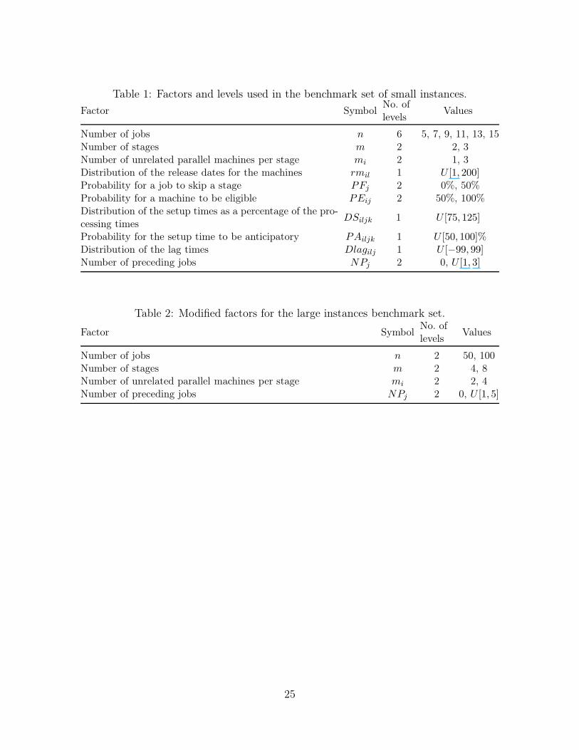
Table 1: Factors and levels used in the benchmark set of small instances.

Factor SymbolNo. oflevels

Values

Number of jobs n 6 5, 7, 9, 11, 13, 15Number of stages m 2 2, 3Number of unrelated parallel machines per stage mi 2 1, 3Distribution of the release dates for the machines rmil 1 U [1, 200]Probability for a job to skip a stage PFj 2 0%, 50%Probability for a machine to be eligible PEij 2 50%, 100%Distribution of the setup times as a percentage of the pro-cessing times

DSiljk 1 U [75, 125]

Probability for the setup time to be anticipatory PAiljk 1 U [50, 100]%Distribution of the lag times Dlagilj 1 U [−99, 99]Number of preceding jobs NPj 2 0, U [1, 3]

Table 2: Modified factors for the large instances benchmark set.

Factor SymbolNo. oflevels

Values

Number of jobs n 2 50, 100Number of stages m 2 4, 8Number of unrelated parallel machines per stage mi 2 2, 4Number of preceding jobs NPj 2 0, U [1, 5]

25

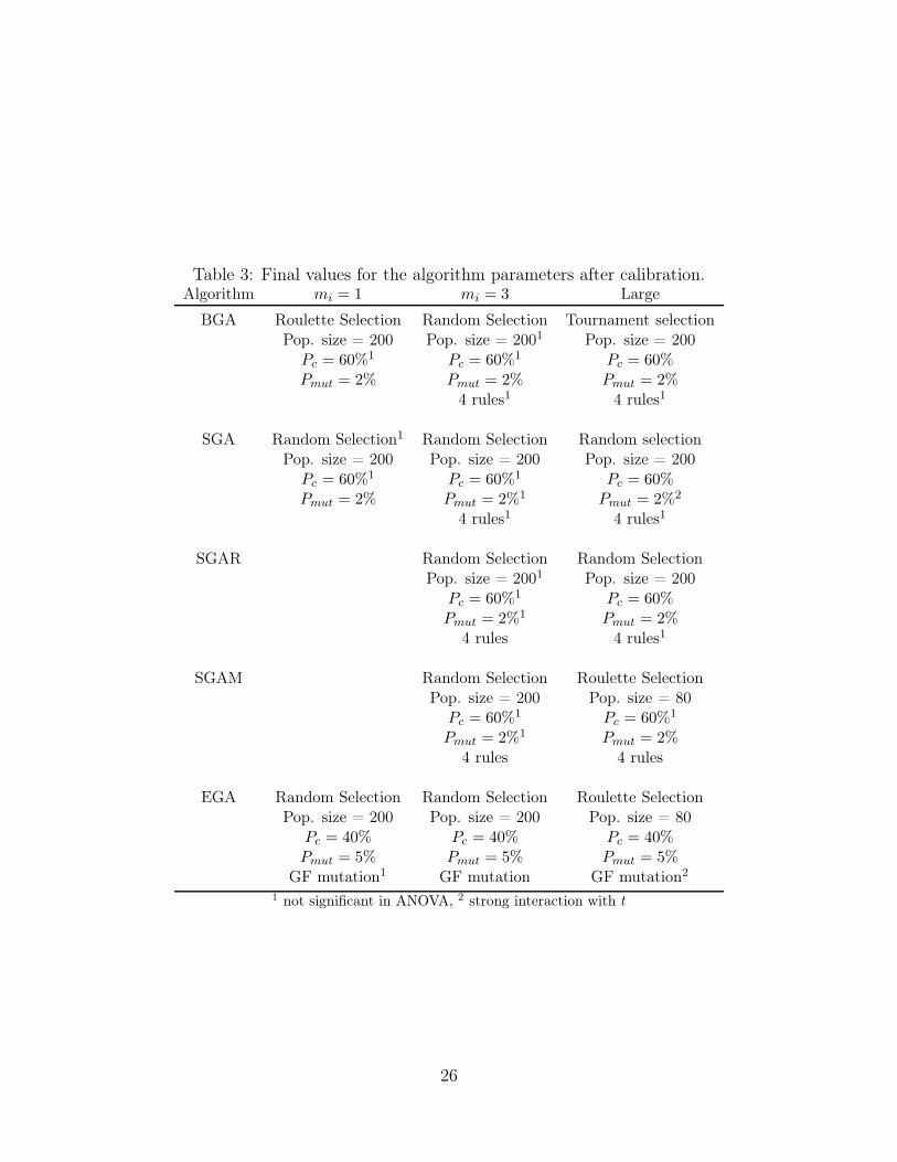
Table 3: Final values for the algorithm parameters after calibration.Algorithm mi = 1 mi = 3 Large

BGA Roulette Selection Random Selection Tournament selectionPop. size = 200 Pop. size = 2001 Pop. size = 200

Pc = 60%1 Pc = 60%1 Pc = 60%Pmut = 2% Pmut = 2% Pmut = 2%

4 rules1 4 rules1

SGA Random Selection1 Random Selection Random selectionPop. size = 200 Pop. size = 200 Pop. size = 200

Pc = 60%1 Pc = 60%1 Pc = 60%Pmut = 2% Pmut = 2%1 Pmut = 2%2

4 rules1 4 rules1

SGAR Random Selection Random SelectionPop. size = 2001 Pop. size = 200

Pc = 60%1 Pc = 60%Pmut = 2%1 Pmut = 2%

4 rules 4 rules1

SGAM Random Selection Roulette SelectionPop. size = 200 Pop. size = 80

Pc = 60%1 Pc = 60%1

Pmut = 2%1 Pmut = 2%4 rules 4 rules

EGA Random Selection Random Selection Roulette SelectionPop. size = 200 Pop. size = 200 Pop. size = 80

Pc = 40% Pc = 40% Pc = 40%Pmut = 5% Pmut = 5% Pmut = 5%

GF mutation1 GF mutation GF mutation2

1 not significant in ANOVA, 2 strong interaction with t

26

Time

Machine 1

Machine 2

Machine 3

Machine 4

3

1

4

4Stage 1

Stage 3

1

Stage 2

Machine 5

3

1

5

5

Setup

2

2

Job 3 Job 4Job 2 Job 5Job 1rmil

Figure 1: Example of a feasible schedule for the HFFL problem studied in this paper.

27

Job permutation

4 3 5 218

Assignment rule

(a) The representation scheme for BGA and SGA

Job permutation 4 3 5 21Assignment rules 1 3 2 46

(b) The solution representation for SGAR

Job permutation 4 3 5 211

Machine assignments 111

23 3 2Stage 1Stage 2

4 54 Stage 3(c) The representation of solutions in SGAM

Machine4 31

Stage Jobs1 1

5

2 2343

1

53

12

54

2

(d) The representation scheme for EGA

Figure 2: An example of the different encodings used in the genetic algorithms.

28

Means and 99.9 Percent LSD Intervals

Population size

Rela

tive d

evia

tion

50 80 20064677073767982(X 0.001)

Figure 3: Factor means plot and LSD intervals for the population size in SGA. Cali-

bration for large instances.

Interactions and 99.9 Percent LSD Intervals

Pmut

Rela

tive d

evia

tion t

525

38

48

58

68

78(X 0.001)

0.01 0.02

Figure 4: Interaction plot and LSD intervals for the mutation probability and the

allowed running time for SGA. Calibration for large instances.

29

Interactions and 99.9 Percent Scheffe Intervals

Algorithm

Relat

ive d

eviat

ion PEij

50%100%

0

0.02

0.04

0.06

0.08

0.1

BGAEGA

SGASGAM

SGAR

Figure 5: Interaction plot and Scheffe intervals for the percentage of skipped stages and

the type of genetic algorithm. Small instances with three machines per stage.

Interactions and 99.9 Percent Scheffe Intervals

Algorithm

Relat

ive d

eviat

ion NPj

0U[1,5]

00.050.1

0.150.2

0.250.3

BGAEGA

SGASGAM

SGAR

Figure 6: Interaction plot and Scheffe intervals for the number of predecessors per job

and the type of genetic algorithm. Large instances.

30

Interactions and 99.9 Percent Scheffe Intervals

Algorithm

Relat

ive d

eviat

ion t

525125

0

0.04

0.08

0.12

0.16

0.2

0.24

BGAEGA

SGASGAM

SGAR

Figure 7: Interaction plot and Scheffe intervals for the allowed running time and the

type of genetic algorithm. Large instances.

Means and 99.9 Percent Scheffe Intervals

Method

Relat

ive d

eviat

ion

BGAEGA

LPTLWR

MIPMWRMWRST

NEHRS

SGASGAM

SGARSPT

0

0.1

0.2

0.3

0.4

Figure 8: Means plot and Scheffe intervals for all methods. Small instances with three

machines per stage.

31

Means and 99.9 Percent Scheffe Intervals

Method

Relat

ive d

eviat

ion

BGAEGA

LPTLWR

MWRMWRST

NEHRS

SGASGAM

SGARSPT

0

0.4

0.8

1.2

1.6

2

2.4

Figure 9: Means plot and Scheffe intervals for all methods. Large instances.

32