Genetic Algorithm Methodology for the Estimation of ...

applied sciences

Article

Genetic Algorithm Methodology for the Estimation ofGenerated Power and Harmonic Content inPhotovoltaic Generation

David A. Elvira-Ortiz 1 , Arturo Y. Jaen-Cuellar 1, Daniel Morinigo-Sotelo 2 ,Luis Morales-Velazquez 1 , Roque A. Osornio-Rios 1 and Rene de J. Romero-Troncoso 1,*

1 HSPdigital—CA Mecatronica, Facultad de Ingenieria, Universidad Autonoma de Queretaro, Campus SanJuan del Rio, Rio Moctezuma 249, Col. San Cayetano, San Juan del Rio C. P. 76807, Queretaro, Mexico;[email protected] (D.A.E.-O.); [email protected] (A.Y.J.-C.); [email protected] (L.M.-V.);[email protected] (R.A.O.-R.)

2 HSPdigital—Research Group ADIRE, University of Valladolid, UVa., Paseo del Cauce, 59, 47011 Valladolid,Spain; [email protected]

* Correspondence: [email protected]

Received: 11 November 2019; Accepted: 7 January 2020; Published: 11 January 2020�����������������

Abstract: Renewable generation sources like photovoltaic plants are weather dependent and it ishard to predict their behavior. This work proposes a methodology for obtaining a parameterizedmodel that estimates the generated power in a photovoltaic generation system. The proposedmethodology uses a genetic algorithm to obtain the mathematical model that best fits the behavior ofthe generated power through the day. Additionally, using the same methodology, a mathematicalmodel is developed for harmonic distortion estimation that allows one to predict the produced powerand its quality. Experimentation is performed using real signals from a photovoltaic system. Eightdays from different seasons of the year are selected considering different irradiance conditions toassess the performance of the methodology under different environmental and electrical conditions.The proposed methodology is compared with an artificial neural network, with the results showingan improved performance when using the genetic algorithm methodology.

Keywords: genetic algorithms; parameter estimation; photovoltaic systems; power quality; totalharmonic distortion

1. Introduction

The smart grid concept involves the inclusion of renewable sources of electric generation andthe use of devices for control and communication, leading to a more efficient and reliable electricsupply for final users [1]. Among all renewable energies, solar photovoltaic (PV) is the one with thehighest growth, reaching an installed worldwide capacity of 402 GW in 2017 [2]. Notwithstanding,there are some challenges and disadvantages associated with photovoltaic generation, for instance,the generated power is unpredictable because it is highly dependent on environmental factors likethe incident solar irradiance and the temperature [3,4]. Additionally, it has been reported that theinclusion of PV generation is associated with harmonic contamination [5,6], because it is necessary touse power inverters for converting the DC signals delivered by the PV panels into AC signals, whichcan be used by the final users. It is necessary to note that even small variations in the backgroundconditions may lead to a severe harmonic contamination, making the constant detection of thesevariations essential [7]. From the smart grid point of view, these are major issues, as the variabilitymakes the generation process unreliable, and the harmonic content compromises the quality of thepower supply. In this sense, several methodologies have been reported for the proper measurement

Appl. Sci. 2020, 10, 542; doi:10.3390/app10020542 www.mdpi.com/journal/applsci

Appl. Sci. 2020, 10, 542 2 of 14

and identification of harmonics. These methodologies use signal processing techniques like discreteFourier transform (DFT) [8], chirp-z transform [9], phasor measurement units [10], Kalman filter basedtechniques [11], and discrete wavelet transform [12]. Although these methodologies offer a solution,they do not provide information regarding the source of the harmonic currents. Moreover, they cannotprovide a model for describing or estimating the behavior of the harmonic content under differentoperating conditions.

In terms of PV generation, there are works focused on the prediction of the power delivered bya PV system [13]. All these methodologies aim to develop models for describing the PV system’sproduction using deterministic or probabilistic techniques [14,15]. However, methods for irradianceand power forecasting based on artificial intelligence have recently gained popularity, being supportvector machines [16], support vector regression [17], and artificial neural networks (ANN) [18–20]the most common techniques used for this purpose. These methodologies can predict the behaviorof any variable on a daily or hourly basis. Nevertheless, these works only perform an estimationof the generated power, and do not deliver information regarding the quality of the generation.Additionally, the use of other metaheuristic methodologies (a set of procedures that do not followa formal mathematical model but a series of empirical rules applied to the search of an optimalvalue), like genetic algorithms (GA), has not been studied. This technique can be used for obtaining amathematical model that describes the behavior of electrical variables in PV generation. Furthermore,the use of GA could help to achieve a parameterized model, in a multioptimization scheme, whichdescribes the behavior of any variable in the PV process even when this behavior presents nonlinearcharacteristics. Moreover, the electrical performance cannot be described using only one parameter,and the GA allows one to obtain several parameters in the same operation.

Some works have included these metaheuristic techniques for solving problems in which theperformance in the PV generation needs to be improved. For instance, maximum power point tracking(MPPT) is a problem in which classical techniques meet difficulties when partial shading conditions(PSC) provide the PV system with a nonmonotonic characteristic of the power–voltage curve [21–23].Therefore, solutions based on particle swarm optimization (PSO), ant colony optimization (ACO),and simulated annealing (SA) have been proposed. However, some of the limitations include theinitial parameters required for the optimization, the amount of data required from the PV grid for acorrect search, and the validation through controlled simulations without considering real variations ofexternal factors. In other works, the GA and the PSO are used to define the best topology of electricaldevices for optimizing commercial building microgrids [24]; yet, these solutions need to be adaptedfor the particular microgrid and the specific user requirements. Finally, metaheuristic techniques havebeen used in the identification of model parameters of PV generation systems for simulation anddesign purposes, such as the crow search algorithm (CSA) [25] and the whale optimization algorithm(WOA) [26]. Nevertheless, in both cases, the validation of the estimation of the mathematical model isperformed through simulations. Therefore, the use of these modern optimization techniques might behelpful if applied to explore the PQ analysis of PV generation systems in the predictive modeling field.Thus, there exists a need for developing methodologies that help in the optimization of models for theprediction of the generation process, including its quality.

This work proposes the use of GA for parameterizing mathematical models that can estimatethe power delivered by a PV system and the level of distortion in the voltage signals associatedwith harmonic contamination. The use of four different parameters to fit the mathematical models isproposed: sun irradiance, cell temperature, DC voltage, and DC current. The proposed methodologywas applied to signals from a real PV generation plant. Experimentation was performed during ayear, and a significant sample of 8 days was taken for its analysis. These days were selected to berepresentative cases of the four seasons of the year with different weather conditions. Results provethat sun irradiance, cell temperature, DC voltage, and DC current can describe the behavior of thepower delivered by the PV inverter, and also the behavior of the total harmonic distortion (THD) inPV generation. Moreover, the resulting models were compared with the results from an ANN, which

Appl. Sci. 2020, 10, 542 3 of 14

is one of the most common techniques in forecasting tasks. It is demonstrated that the estimationsperformed by the GA are better than those delivered by the ANN.

2. Theoretical Background

This section introduces the theoretical background for the implementation of theproposed methodology.

2.1. Active Power Definition

The standard IEEE std. 1459–2010 [27] defines the active power (P) as the average value of theinstantaneous power during a time interval τ, as shown in (1):

P =1τ

∫ τ

0p(t)dt, (1)

where p(t) = v(t) ∗ i(t) is the instantaneous power. Equation (1) can be discretized resulting in (2):

P =1τ

∑N

k=1v(k)i(k), (2)

where N is the number of samples comprising the time interval τ ; and v(k) and i(k) are the k -thelement of the voltage and current signals, respectively.

2.2. Total Harmonic Distortion (THD)

According to the standard IEEE 519–2014 [28], harmonics are sinusoidal components in voltagesignals that have frequencies that are integer multiples of the fundamental frequency component.Harmonic components are related to waveform distortion and the level of distortion due to harmonicsis quantified using the THD index. The mathematical expression for THD is presented in (3):

THD =

√∑50h=2 Ph

2

P1100, (3)

where P1 is the power of the fundamental component and Ph is the power of the harmonic componentof order h. The power of the harmonic components is found using the Fourier transform. The THDcalculation must be performed using a 200 ms time window, i.e., 12 cycles for 60 Hz power systems or10 cycles for 50 Hz power systems.

2.3. Evolutionary-Based Algorithm

Genetic algorithms (GA) are used in this work since they can be easily adjusted to this particularproblem with some advantages over other evolutionary-based algorithms. For instance, GA keep apopulation of potential solutions, whereas other techniques work with a single variable. Anotherbenefit is their concept simplicity and their easiness of implementation [29]. GA are a set of elementsbased on Darwin’s theory of survival of the fittest. The following five features, applied in an iterativeprocess, allow the GA to be a functional optimization search: (i) design variable coding; (ii) objectivefunction and fitness value; (iii) selection mechanism and genetic operators; (iv) crossover; and (v)mutation [30]. It is worth understanding how the technique works. In natural genetics, a group ofchromosomes (or individuals) make up the population to be evolved (converged); therefore, eachindividual is integrated by genes, which represent the design variables to be optimized (or searched for).

According to [29], the next steps illustrate a general form in which GA are implemented:Step 1: Definition of general parameters, according to the problem to be solved, and generation

of a random initial population (potential solutions).

Appl. Sci. 2020, 10, 542 4 of 14

Step 2: Evaluation of the population by substituting the potential solution in an objective functionthat calculates the fitness value, which evaluates quantitatively how good every individual is.

Step 3: Performance of an elitist selection of the best individuals according to the fitness value forreproduction purposes with the genetic operators: crossover and mutation.

Step 4: Evaluation of the termination criteria for the iterative process, and if they are satisfied,then go to Step 8, where the best solutions are presented; otherwise, go to Step 5.

Step 5: Generation of a new population by applying the crossover operation to the selectedindividuals in Step 3. This ensures evolution (convergence) of the possible solutions.

Step 6: Generation of population diversity, and local trapping scape, by applying the mutationoperation according to a mutation probability to avoid losing valuable information.

Step 7: Replacement of the initial population with the new population obtained through Steps 5and 6 and go to Step 2.

Step 8: Return the best solutions obtained.

3. Methodology

3.1. Parameterization Dataset and Experimentation Dataset

In this work, two different datasets are used: one for parameterization and one for experimentation.The parameterization dataset takes into account a year from which two different days per every monthare selected, comprising a total of 24 days. The criteria for selecting the two days of each month are asfollows: one day with almost no irradiance variations associated with cloud presence; and a secondday with cloud presence that generates unexpected variations in the irradiance profile. This datasetis only used for the estimation of the parameters of every model (active power and THD). Once theparameters of the model are estimated, a different dataset is used for experimentation. On the otherhand, 8 days, taken through the year, are analyzed to form the experimentation dataset. Each one ofthese days is different from those selected for the parameterization dataset. This selection is performedconsidering the following: two representative days per season of the year are selected to assess themodel under different environmental conditions. Moreover, for each season, one day with only a fewclouds through the day (or none if it is possible) is selected. For the second day of each season, onewith many abrupt irradiance variations due to cloud presence is selected. In this way, it is possible toassess the performance of the methodology under different scenarios.

3.2. Genetic Algorithm for the Parameter Estimation

A general block diagram of the proposed methodology is presented in Figure 1. First, a GAscheme is used for the active power forecasting of a PV inverter. This scheme requires the followinginputs: sun irradiance, cell temperature, DC voltage, DC current, an active power signal, and thenon-parameterized mathematical model, which works as the objective function. These descriptiveparameters are selected considering that PV panels deliver energy in DC levels depending on theenvironmental factors. The objective function for this task is presented in (4). This mathematical modelis selected because it is observed that the relationship between the solar irradiance and the activepower tends to be proportional [31,32].

Pi = w1x1,i + w2x2,i + w3x3,i + w4x4,i, (4)

where Pi is the i-th value of the estimated active power;

x1,i is the i-th value of the sun irradiance;x2,i is the i-th value of the cell temperature;x3,i is the i-th value of the DC voltage signal;x4,i is the i-th value of the DC current signal; andw1, w2, w3, and w4 are constant weights determined by the GA.

Appl. Sci. 2020, 10, 542 5 of 14

Every weight in (4) specifies the level of contribution of each variable in the description of thebehavior at the response function. It must be said that the relationship between the descriptiveparameters and the obtained result is not linear in all cases, but in this work, we propose to developa model that linearizes this relationship in order to allow for a simple solution to the problem. It isclear that this situation introduces an error in the estimation; however, the GA must be able to findthe weights that minimize this error in order to obtain accurate results. Once all the inputs have beendefined, the next step consisted of the initialization of the GA. For this particular case, the parametersthat must be defined by the GA are w1, w2, w3, and w4. Therefore, a random initial population of 50individuals is generated for each weight, this way a good design space distribution is ensured. This isfollowed by an evaluation of the population, which consists of substituting the value of each individualon the objective function and determining the error with respect to the active power signal.

Appl. Sci. 2020, 10, x FOR PEER REVIEW  5  of  13 

clear that this situation introduces an error in the estimation; however, the GA must be able to find 

the weights that minimize this error in order to obtain accurate results. Once all the inputs have been 

defined,  the  next  step  consisted  of  the  initialization  of  the  GA.  For  this  particular  case,  the 

parameters  that must be defined by  the GA  are 𝑤 , 𝑤 , 𝑤 ,  and 𝑤 . Therefore,  a  random  initial 

population of 50 individuals is generated for each weight, this way a good design space distribution 

is ensured. This is followed by an evaluation of the population, which consists of substituting the 

value of  each  individual on  the objective  function and determining  the  error with  respect  to  the 

active power signal. 

Figure 1. Block diagram of the proposed methodology. THD: Total Harmonic Distortion;  𝑃 : i‐th 

element of the Active Power; 𝐻 : i‐th element of the harmonic distortion;  𝑥 𝑤 ：Elements of 

equation (4) 

Subsequently, a selection process  is carried out. For  this process,  the obtained error  for each 

individual is used to organize them from the best fitting (the individual with the least error) to the 

worst fitting (the individual with the highest error). At this point, it is necessary to evaluate if the 

stop criterion has been reached; hence, the best fitting individual is taken as the solution. Otherwise, 

it is necessary to generate a new population. In this work the stop criterion is a maximum number of 

epochs  set  as  500,  because  it  is  experimentally  observed  that  this  number  ensures  the  best 

convergence  of  the model parameters. To  generate  the  new population,  the  individual with  the 

lowest error is preserved, in this manner, the convergence of the algorithm is granted. The rest of the 

individuals  in  the  new  population  are  obtained  through  two  different  genetic  operations:  the 

crossover  and  the mutation.  The  crossover  operation  consists  of  the  average  of  the  best  fitting 

individual with the rest of the individuals, one at a time, as shown in (5): 

𝑦 ,, ,  (5) 

where  𝑖 2, 3, … ,50; 𝑦 ,   is the i‐th individual of the old population; 

𝑦   is the best fitting individual; and 𝑦 ,   is the i‐th individual of the new population. 

The mutation operation  implies a  random  substitution of a particular  individual of  the new 

population. The individual is substituted if a random value lies below the mutation probability (0.2 

in  this  work)  to  maintain  diversity  in  the  population,  but  without  losing  valuable  genetic 

information. Once the new population is obtained, the process is repeated from the evaluation step 

as long as the stop criterion is not reached. When the stop criterion is reached, the GA delivers the 

estimated parameterized model for the active power forecasting. In the case of the THD prediction, 

Figure 1. Block diagram of the proposed methodology. THD: Total Harmonic Distortion; Pi: i-thelement of the Active Power; Hi: i-th element of the harmonic distortion; xiwi: Elements of Equation (4).

Subsequently, a selection process is carried out. For this process, the obtained error for eachindividual is used to organize them from the best fitting (the individual with the least error) to theworst fitting (the individual with the highest error). At this point, it is necessary to evaluate if the stopcriterion has been reached; hence, the best fitting individual is taken as the solution. Otherwise, itis necessary to generate a new population. In this work the stop criterion is a maximum number ofepochs set as 500, because it is experimentally observed that this number ensures the best convergenceof the model parameters. To generate the new population, the individual with the lowest error ispreserved, in this manner, the convergence of the algorithm is granted. The rest of the individualsin the new population are obtained through two different genetic operations: the crossover and themutation. The crossover operation consists of the average of the best fitting individual with the rest ofthe individuals, one at a time, as shown in (5):

yi,new =(y1 + yi, old)

2, (5)

where i = 2, 3, . . . , 50;

yi, old is the i-th individual of the old population;y1 is the best fitting individual; andyi,new is the i-th individual of the new population.

Appl. Sci. 2020, 10, 542 6 of 14

The mutation operation implies a random substitution of a particular individual of the newpopulation. The individual is substituted if a random value lies below the mutation probability (0.2 inthis work) to maintain diversity in the population, but without losing valuable genetic information.Once the new population is obtained, the process is repeated from the evaluation step as long as the stopcriterion is not reached. When the stop criterion is reached, the GA delivers the estimated parameterizedmodel for the active power forecasting. In the case of the THD prediction, the aforementioned processis carried out with only two differences. The first is related to the objective function. For the THDmodel, Equation (6) is used:

Hi = u1x1, i + u2x2,i + u3x3,i + u4x4,i + u5x5,i + u6x6,i + u7x7,i + u8x8,i + u9x9,i+

u10x10,i + u11x11,i + u12x12,i + u13x13,i + u14x14,i,(6)

where Hi is the i-th value of the estimated THD;

x1,i is the i-th value of the sun irradiance;x2,i is the i-th value of the cell temperature;x3,i is the i-th value of the DC voltage signal;x4,i is the i-th value of the DC current signal;x5,i = x1,ix2,i ;x6,i = x1,ix3,i;x7,i = x1,ix4,i;x8,i = x2,ix3,i;x9,i = x2,ix4,i;x10,i = x3,ix4,i;x11,i = x1,ix1,i;x12,i = x2,ix2,i ;x13,i = x3,ix3,i;x14,i = x4,ix4,i; and

u1, u2, u3, u4, u5, u6, u7, u8, u9, u10, u11, u12, u13, and u14 are the constant weights determined bythe GA.

The objective function for the THD forecasting is selected in this way because Equation (3) is anexpression that involves quadratic terms; therefore, these types of terms should be considered in themodel for the estimation. Moreover, electric parameters are not conventionally related with the THD.However, in this case, the voltage and currents signals represent an important part of the internalbehavior of the PV system and this is why their use in the estimation of THD is being proposed only inthe PV generation process. To obtain the THD prediction, the GA is trained using THD testing signals.With these two modifications (objective function and test signal), it is possible to perform the THDprediction. The methodology is performed a total of 24 times, one for each day of the parameterizationdataset. The final weights for the two models are the average of these 24 results. Finally, the proposedmethodology is used to perform the forecasting of the active power and the THD of eight differentdays from those used for the estimation of the parameterized model. These days come from fourdifferent seasons of the year, and they present different weather conditions from each other. This way,it is possible to evaluate the variability associated with the specific climatic changes of each season, butalso the variability that results from the lack of sunlight when there are clouds in the sky.

3.3. Piecewise Approach of the Proposed Methodology

Since it has been demonstrated that a PV inverter has an anomalous behavior when it operates inregions far from its rated values [33], the described methodology is applied considering the signals in apiecewise approach. Therefore, the design variables and the objective function are divided into foursections through a day. Considering that the maximum expected irradiance value is around the 1000

Appl. Sci. 2020, 10, 542 7 of 14

W/m2, a threshold of the 20% of this value is set for defining two regions: one at the beginning andanother at the end of the day. These two sections are named S1 and S4, and they are the regions wherethe values of the irradiance are below the threshold value, i.e., they represent the low power operationregions of the PV inverter. The remaining data of the signals are divided into halves to obtain twoother sections called S2 and S3. This way, a total of four sections (S1, S2, S3, and S4) are obtained and adifferent set of weights is estimated for each one.

4. Experimental Setup

Experimentation was performed with real signals coming from a PV generation plant located incentral Spain, at a latitude of 39◦36’N and a longitude of 02◦05’W. Measurements were performed in a100 kW installation that uses an Ingecon Sun 100 solar inverter. Herein, a set of polycrystalline siliconPV panels on the DC side of the PV inverter was located, which delivered a peak power of 125 kW. ThePV panels are south facing and present a tilt angle β = 45◦. The global irradiance that reaches the PVpanels was measured using a calibrated PV reference cell that poses the same orientation and tilt angleas the PV panels. The data from both sides of the PV inverter were acquired and collected using aproprietary FPGA-based (Field Programmable Gate Array) data acquisition system (DAS). The DAScan acquire data from seven simultaneous channels at 8000 samples per second (SPS) with a 16-bitresolution. The DAS on the DC side was designed for measuring voltages up to 1000 V and for workingwith any current clamp that delivers a ±4 V output. On this side, only two channels are required: onefor the voltage and another one for the current. The clamp used for the current measurement is theHOP 500-SB/SP1 by LEM. On the AC side, six channels of the DAS are required to measure the voltageand current of the three phases. Since the PV inverter operates in a low voltage grid, the DAS on thisside was designed for measuring voltages up to 400 Vrms, and for using any current clamp with a ±2V output. The current was taken from a measurement transformer, so SCT-013-010 sensors by YHDCwere used with the DAS. All the voltage signals were acquired using wires directly connected fromthe PV inverter to the DAS. The voltage and current waveforms were stored during an extended timeusing a standard 128 GB micro SD card.

5. Results and Discussion

This section presents the results of applying the proposed methodology for the modelparameterization and the experimentation for the active power and THD estimation.

5.1. Parameterization Results

Firstly, the proposed methodology was applied for parameterizing the active power model andthe THD model, using the piecewise approach previously described. In Table 1, the weights w1, w2,w3, and w4, delivered by the GA using the 24 days of the parameterizing dataset for the four sectionsof the active power estimation, are summarized. It is observed in Table 1 that the weight values arevery different from one section to another; thus, it can be inferred that using the whole signal, insteadof sectioning it, may compromise the accuracy of the results. Additionally, the resulting 14 weightsfor the four sections of the THD signals are presented in Table 2. Once again, the parameterizationdataset was also used to obtain these weights. Just as in the previous case, all the values significantlyvary from one section of the THD signal to another, confirming the fact that the piecewise approachimplemented in this work helps to increase the reliability of the methodology. As aforementioned, thebehavior of the PV system is different depending on the operating conditions [33], i.e., the behavior ofthe system is nonlinear. This nonlinearity is the main reason for the variation in the weights presentedin the different sections of the estimated models.

Appl. Sci. 2020, 10, 542 8 of 14

Table 1. Estimated weights for the four sections of the active power model.

Weight S1 S2 S3 S4

w1 34.23 25.13 7.57 −1.92w2 7.14 −55.62 75.85 −24.83w3 −1.19 1.06 −6.25 0.98w4 −63.16 37.39 103.43 120.92

Table 2. Estimated weights for the four sections of the total harmonic distortion (THD) model.

Weight S1 S2 S3 S4

u1 −3.27 −1.92 0.19 2.59u2 4.92 3.77 −0.86 1.84u3 1.38 0.85 −2.06 −0.94u4 −4.68 3.63 −0.44 0.85u5 0.03 −0.19 −2.06 −3.99u6 4.45 −0.86 0.16 −0.22u7 −1.54 0.13 2.21 −0.92u8 0.50 0.25 2.25 −0.65u9 −0.92 −2.12 −1.96 −1.93u10 −1.89 −0.62 −0.69 −3.05u11 2.66 0.31 −0.16 −2.22u12 −0.39 −2.18 3.29 4.04u13 −3.08 −0.13 1.55 −1.67u14 −4.93 0.77 1.78 −1.22

5.2. Experimentation Results

In order to demonstrate that the proposed methodology delivers similar and uniform output data,it is necessary to perform a comparison with 2 sunny days and 2 cloudy days of the same month. Inthis sense, 4 days were randomly selected from the month of August, because in this month it is easyto find suitable days that match these characteristics (sunny and cloudy). The weights presented inTable 1 were used to estimate the delivered active power of these 4 days, and the results are presentedin Figure 2.

Appl. Sci. 2020, 10, x FOR PEER REVIEW  8  of  13 

Table 2. Estimated weights for the four sections of the total harmonic distortion (THD) model. 

Weight  S1  S2  S3  S4 

u1  −3.27  −1.92  0.19  2.59 

u2  4.92  3.77  −0.86  1.84 

u3  1.38  0.85  −2.06  −0.94 

u4  −4.68  3.63  −0.44  0.85 

u5  0.03  −0.19  −2.06  −3.99 

u6  4.45  −0.86  0.16  −0.22 

u7  −1.54  0.13  2.21  −0.92 

u8  0.50  0.25  2.25  −0.65 

u9  −0.92  −2.12  −1.96  −1.93 

u10  −1.89  −0.62  −0.69  −3.05 

u11  2.66  0.31  −0.16  −2.22 

u12  −0.39  −2.18  3.29  4.04 

u13  −3.08  −0.13  1.55  −1.67 

u14  −4.93  0.77  1.78  −1.22 

5.2. Experimentation Results 

In order to demonstrate that the proposed methodology delivers similar and uniform output 

data,  it  is necessary  to perform a  comparison with 2  sunny days and 2  cloudy days of  the  same 

month.  In  this  sense, 4 days were  randomly  selected  from  the month of August, because  in  this 

month  it  is  easy  to  find  suitable  days  that match  these  characteristics  (sunny  and  cloudy).  The 

weights presented in Table 1 were used to estimate the delivered active power of these 4 days, and 

the results are presented in Figure 2. 

Figure 2. Comparison of two sunny days: (a) 13 August and (b) 14 August; and two cloudy days: (c) 

15 August and (d) 17 August; for the demonstration of data similarity and uniformity. 

From Figure 2, it is observed that when the days are sunny, the estimated and the real active 

power are very similar  (see Figure 2a,b),  reaching an estimation error of 0.1%  for 13 August and 

0.37% for 14 August. The difference between both errors is less than 0.3%, proving the consistency of 

the results delivered by the methodology. In the case of the cloudy days (Figure 2c,d), the cloudy 

nature of the days causes a high variability in the generated power. However, the methodology is 

able to follow most of the variations in a reasonable way reaching an error of 0.39% for 15 August 

and 0.56%  for 17 August. This  time  the difference between both errors  is even  lower  than  in  the 

Figure 2. Comparison of two sunny days: (a) 13 August and (b) 14 August; and two cloudy days:(c) 15 August and (d) 17 August; for the demonstration of data similarity and uniformity.

Appl. Sci. 2020, 10, 542 9 of 14

From Figure 2, it is observed that when the days are sunny, the estimated and the real activepower are very similar (see Figure 2a,b), reaching an estimation error of 0.1% for 13 August and 0.37%for 14 August. The difference between both errors is less than 0.3%, proving the consistency of theresults delivered by the methodology. In the case of the cloudy days (Figure 2c,d), the cloudy nature ofthe days causes a high variability in the generated power. However, the methodology is able to followmost of the variations in a reasonable way reaching an error of 0.39% for 15 August and 0.56% for 17August. This time the difference between both errors is even lower than in the previous case (<0.2%).In this way, it is possible to validate the similarity and uniformity of the resulting data for days withsimilar characteristics.

As aforementioned, 8 days were used for experimentation with the proposed methodology in thepiecewise approach. These days are presented in Figure 3 with the corresponding sections of the day(S1 to S4). The values of the irradiance are overall normalized in order to better appreciate the averagetendency of every season of the year. It can be seen that the highest values are reached in spring, butthey are sudden and last only a few minutes. The lowest values occur in winter; this situation is mainlydue to the elevation of the sun in this season being the lowest of the year. Additionally, it is observedthat there is a great variability between them because of the different environmental conditions. Thefirst season presented in Figure 3 is summer, characterized by an abundance of sun and a few cloudyperiods. The first day of this season is a completely sunny day (there is none irradiance variation),whereas the second day presents some unexpected variations (due to clouds) from the 12:00 to the 15:00(see Figure 3a). The second season is autumn; here, the first day presents a few variations associatedwith cloud presence, whereas the second presents a storm during the second half of the day resultingin many abrupt irradiance variations (Figure 3b). The third season presented in the figure is winter;here, the first day (Figure 3c) presents a profile very similar to the first day of summer. However, it isobserved that the total sunny hours are lower in winter. The highest irradiance level reached is alsolower in winter than summer. The second day of winter shows a very irregular pattern because thereis cloud presence during the entire day. Finally, the fourth and last presented season is spring. The firstday presents a normal pattern of behavior for most of the day, but around the 17:00 it becomes cloudyand some variations in irradiance appear (Figure 3d). The second day of spring presents an erraticbehavior since there are clouds all day. The weight values presented in Table 1 were substituted into (4)along with the irradiance, cell temperature, DC voltage, and DC current from every one of the sections.

Appl. Sci. 2020, 10, x FOR PEER REVIEW  9  of  13 

previous  case  (<0.2%).  In  this way,  it  is possible  to validate  the  similarity  and uniformity of  the 

resulting data for days with similar characteristics. 

As aforementioned, 8 days were used for experimentation with the proposed methodology in 

the piecewise approach. These days are presented in Figure 3 with the corresponding sections of the 

day (S1 to S4). The values of the irradiance are overall normalized in order to better appreciate the 

average tendency of every season of the year. It can be seen that the highest values are reached in 

spring, but  they are sudden and  last only a  few minutes. The  lowest values occur  in winter;  this 

situation  is mainly  due  to  the  elevation  of  the  sun  in  this  season  being  the  lowest  of  the  year. 

Additionally,  it  is observed  that there  is a great variability between  them because of  the different 

environmental  conditions. The  first  season presented  in Figure 3  is  summer,  characterized by an 

abundance of sun and a few cloudy periods. The first day of this season is a completely sunny day 

(there  is none  irradiance variation), whereas  the second day presents some unexpected variations 

(due to clouds) from the 12:00 to the 15:00 (see Figure 3a). The second season is autumn; here, the 

first day presents a  few variations associated with cloud presence, whereas  the second presents a 

storm during the second half of the day resulting in many abrupt irradiance variations (Figure 3b). 

The third season presented in the figure is winter; here, the first day (Figure 3c) presents a profile 

very similar to the first day of summer. However, it is observed that the total sunny hours are lower 

in winter. The highest irradiance level reached is also lower in winter than summer. The second day 

of winter  shows  a very  irregular pattern  because  there  is  cloud presence during  the  entire day. 

Finally,  the  fourth and  last presented season  is spring. The  first day presents a normal pattern of 

behavior  for most  of  the  day,  but  around  the  17:00  it  becomes  cloudy  and  some  variations  in 

irradiance appear (Figure 3d). The second day of spring presents an erratic behavior since there are 

clouds  all day. The weight values presented  in Table  1 were  substituted  into  (4)  along with  the 

irradiance, cell temperature, DC voltage, and DC current from every one of the sections. 

Figure  3. Days  of  analysis  for  (a)  summer,  (b)  fall,  (c) winter,  and  (d)  spring, with  normalized 

irradiance. 

Then, the estimation of the active power for the 8 days of analysis was carried out. In order to 

show the effectiveness of  the proposed methodology, the performed estimation  is compared with 

the estimation performed with an ANN, which is the most common technique for this purpose. The 

ANN was trained using the same 24 days that were used for estimating the parameterized model 

with the GA. Figure 4 shows the results of the active power estimation using these two techniques. It 

is observed that in the 8 days, the value estimated by the GA (red line) remains very close to the real 

Figure 3. Days of analysis for (a) summer, (b) fall, (c) winter, and (d) spring, with normalized irradiance.

Appl. Sci. 2020, 10, 542 10 of 14

Then, the estimation of the active power for the 8 days of analysis was carried out. In order toshow the effectiveness of the proposed methodology, the performed estimation is compared with theestimation performed with an ANN, which is the most common technique for this purpose. The ANNwas trained using the same 24 days that were used for estimating the parameterized model with the GA.Figure 4 shows the results of the active power estimation using these two techniques. It is observed thatin the 8 days, the value estimated by the GA (red line) remains very close to the real value (blue line).Although there are days with many unexpected variations like 13 November (Figure 4d), 10 February(Figure 4f), and 21 March (Figure 4h), the obtained model can follow every variation reasonably. In thedays where there are no abrupt changes, the difference between the estimated and the real value isalmost imperceptible. When an ANN is used for the active power forecasting, the results are also good(yellow line). The prediction accurately follows the behavior shown by the real signal on most of thedays. However, it is observed that for 9 January (Figure 4e), the estimation performed by the ANNpresents a noticeable deviation from the real signal. In this sense, the estimation performed by the GAdoes not present this deviation making it a more reliable technique.

Appl. Sci. 2020, 10, x FOR PEER REVIEW  10  of  13 

value  (blue  line). Although  there  are  days with many  unexpected  variations  like  13 November 

(Figure 4d), 10 February (Figure 4f), and 21 March (Figure 4h), the obtained model can follow every 

variation  reasonably.  In  the days where  there are no abrupt  changes,  the difference between  the 

estimated and the real value  is almost  imperceptible. When an ANN  is used for the active power 

forecasting, the results are also good (yellow  line). The prediction accurately follows the behavior 

shown by the real signal on most of the days. However, it is observed that for 9 January (Figure 4e), 

the estimation performed by the ANN presents a noticeable deviation from the real signal. In this 

sense, the estimation performed by the GA does not present this deviation making it a more reliable 

technique. 

Figure  4. Comparison between  the  real  and  the  estimated  active power  for  (a)  13 August,  (b)  12 

September, (c) 27 October, (d) 13 November, (e) 9 January, (f) 10 February, (g) 20 March, and (h) 21 

March. 

On  the  other  hand,  the  weights  from  Table  2  were  substituted  into  (6)  to  obtain  the 

mathematical model for the THD forecasting. Once again, the result of the estimation performed by 

the GA is compared with the estimation performed by an ANN. The results of using these models 

for estimating the THD through the day are depicted in Figure 5. In the days with almost no cloud 

presence (Figure 5a,c,e,g), the values estimated by  the GA (red  line) present  just a few deviations 

from  the  real ones  (blue  line).  In  the days with severe cloud presence,  the deviation between  the 

estimated values and  the real values  is more noticeable,  i.e.,  the error  in  the estimation  increases. 

However, when an ANN is used for the THD prediction, it is noticeable that the network does not 

make a good estimation even on days when the sky is clear (yellow line). Thus, it can be inferred that 

the  ANN  presents  problems  for  estimations  where  the  relationship  among  the  parameters  is 

nonlinear. The error values  for both  techniques  (GA and ANN) are  summarized  in Table 3.  It  is 

worth  noting  that  the  errors,  for  the  case  of  the  active  power  estimation,  using  the GA  always 

remains in values lower than 1%. As expected, the estimation performed by the ANN presents the 

highest  error  on  9  January,  but  also  10  February,  and  13 November  present  errors  above  1%. 

Meanwhile, in the case of the THD estimation, the errors obtained indicate that when using the GA, 

the estimation error never goes beyond 2%. Regarding the results obtained using the ANN, they are 

very variable, and  the errors  fluctuate between 3.2% and 33.2%, showing  that  the ANN  is not as 

reliable  as  the  GA  for  this  particular  estimation.  The  results  obtained  using  the  proposed 

methodology are meaningful because they show that the proper combination of sun irradiance, cell 

temperature, DC  voltage,  and DC  current  can  reasonably  estimate  the  active  power  of  a whole 

production day in PV systems. However, a more important fact is that the proposed approach can 

also describe  the THD associated with  the generation process. Having a priori knowledge of  the 

quality of a generation process is important from the smart grid point of view in order to guarantee a 

reliable and robust supply. 

Figure 4. Comparison between the real and the estimated active power for (a) 13 August, (b) 12September, (c) 27 October, (d) 13 November, (e) 9 January, (f) 10 February, (g) 20 March, and (h)21 March.

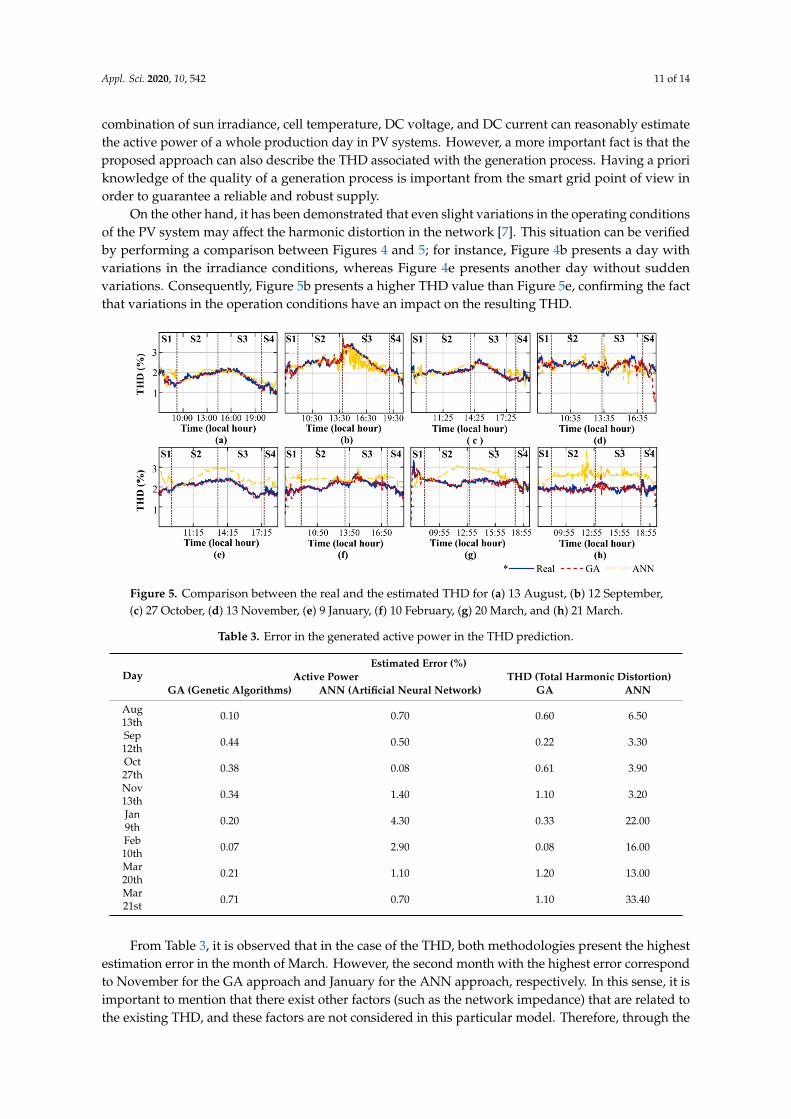
On the other hand, the weights from Table 2 were substituted into (6) to obtain the mathematicalmodel for the THD forecasting. Once again, the result of the estimation performed by the GA iscompared with the estimation performed by an ANN. The results of using these models for estimatingthe THD through the day are depicted in Figure 5. In the days with almost no cloud presence(Figure 5a,c,e,g), the values estimated by the GA (red line) present just a few deviations from the realones (blue line). In the days with severe cloud presence, the deviation between the estimated valuesand the real values is more noticeable, i.e., the error in the estimation increases. However, when anANN is used for the THD prediction, it is noticeable that the network does not make a good estimationeven on days when the sky is clear (yellow line). Thus, it can be inferred that the ANN presentsproblems for estimations where the relationship among the parameters is nonlinear. The error valuesfor both techniques (GA and ANN) are summarized in Table 3. It is worth noting that the errors, forthe case of the active power estimation, using the GA always remains in values lower than 1%. Asexpected, the estimation performed by the ANN presents the highest error on 9 January, but also 10February, and 13 November present errors above 1%. Meanwhile, in the case of the THD estimation,the errors obtained indicate that when using the GA, the estimation error never goes beyond 2%.Regarding the results obtained using the ANN, they are very variable, and the errors fluctuate between3.2% and 33.2%, showing that the ANN is not as reliable as the GA for this particular estimation. Theresults obtained using the proposed methodology are meaningful because they show that the proper

Appl. Sci. 2020, 10, 542 11 of 14

combination of sun irradiance, cell temperature, DC voltage, and DC current can reasonably estimatethe active power of a whole production day in PV systems. However, a more important fact is that theproposed approach can also describe the THD associated with the generation process. Having a prioriknowledge of the quality of a generation process is important from the smart grid point of view inorder to guarantee a reliable and robust supply.

On the other hand, it has been demonstrated that even slight variations in the operating conditionsof the PV system may affect the harmonic distortion in the network [7]. This situation can be verifiedby performing a comparison between Figures 4 and 5; for instance, Figure 4b presents a day withvariations in the irradiance conditions, whereas Figure 4e presents another day without suddenvariations. Consequently, Figure 5b presents a higher THD value than Figure 5e, confirming the factthat variations in the operation conditions have an impact on the resulting THD.

Appl. Sci. 2020, 10, x FOR PEER REVIEW  11  of  13 

On  the  other  hand,  it  has  been  demonstrated  that  even  slight  variations  in  the  operating 

conditions of the PV system may affect the harmonic distortion in the network [7]. This situation can 

be verified by performing a comparison between Figures 4 and 5; for instance, Figure 4b presents a 

day with variations  in the  irradiance conditions, whereas Figure 4e presents another day without 

sudden variations. Consequently, Figure 5b presents a higher THD value than Figure 5e, confirming 

the fact that variations in the operation conditions have an impact on the resulting THD. 

Figure 5. Comparison between the real and the estimated THD for (a) 13 August, (b) 12 September, 

(c) 27 October, (d) 13 November, (e) 9 January, (f) 10 February, (g) 20 March, and (h) 21 March. 

Table 3. Error in the generated active power in the THD prediction. 

Day 

Estimated Error (%) 

Active Power  THD (Total Harmonic Distortion) 

GA (Genetic Algorithms)  ANN (Artificial Neural Network)  GA  ANN 

Aug 13th  0.10  0.70  0.60  6.50 

Sep 12th  0.44  0.50  0.22  3.30 

Oct 27th  0.38  0.08  0.61  3.90 

Nov 13th  0.34  1.40  1.10  3.20 

Jan 9th  0.20  4.30  0.33  22.00 

Feb 10th  0.07  2.90  0.08  16.00 

Mar 20th  0.21  1.10  1.20  13.00 

Mar 21st  0.71  0.70  1.10  33.40 

From Table 3, it is observed that in the case of the THD, both methodologies present the highest 

estimation  error  in  the  month  of  March.  However,  the  second  month  with  the  highest  error 

correspond to November for the GA approach and January for the ANN approach, respectively. In 

this sense, it is important to mention that there exist other factors (such as the network impedance) 

that are related to the existing THD, and these factors are not considered in this particular model. 

Therefore, through the effects of non‐considered factor changes, the accuracy of any methodology 

may be compromised; thus, as has been previously mentioned, the error in the estimation does not 

necessarily  follow  the same  tendency  in both methodologies. This means  that  the accuracy of  the 

estimation  would  depend  on  the  robustness  of  the  used  methodology  to  the  variation  of 

non‐considered parameters.  In  this  case,  the GA methodology  seems  to be more  robust  to  these 

kinds of variations. 

6. Conclusions 

The  contribution of  the present work  is  a novel methodology  that  combines  environmental 

factors  and  PV  generation  variables  to  define  two  models  for  forecasting  the  behavior  of  the 

generated power  and  its harmonic  content  in  a PV generation plant. An  optimization  technique 

Figure 5. Comparison between the real and the estimated THD for (a) 13 August, (b) 12 September,(c) 27 October, (d) 13 November, (e) 9 January, (f) 10 February, (g) 20 March, and (h) 21 March.

Table 3. Error in the generated active power in the THD prediction.

DayEstimated Error (%)

Active Power THD (Total Harmonic Distortion)GA (Genetic Algorithms) ANN (Artificial Neural Network) GA ANN

Aug13th 0.10 0.70 0.60 6.50

Sep12th 0.44 0.50 0.22 3.30

Oct27th 0.38 0.08 0.61 3.90

Nov13th 0.34 1.40 1.10 3.20

Jan9th 0.20 4.30 0.33 22.00

Feb10th 0.07 2.90 0.08 16.00

Mar20th 0.21 1.10 1.20 13.00

Mar21st 0.71 0.70 1.10 33.40

From Table 3, it is observed that in the case of the THD, both methodologies present the highestestimation error in the month of March. However, the second month with the highest error correspondto November for the GA approach and January for the ANN approach, respectively. In this sense, it isimportant to mention that there exist other factors (such as the network impedance) that are related tothe existing THD, and these factors are not considered in this particular model. Therefore, through the

Appl. Sci. 2020, 10, 542 12 of 14

effects of non-considered factor changes, the accuracy of any methodology may be compromised; thus,as has been previously mentioned, the error in the estimation does not necessarily follow the sametendency in both methodologies. This means that the accuracy of the estimation would depend on therobustness of the used methodology to the variation of non-considered parameters. In this case, theGA methodology seems to be more robust to these kinds of variations.

6. Conclusions

The contribution of the present work is a novel methodology that combines environmental factorsand PV generation variables to define two models for forecasting the behavior of the generatedpower and its harmonic content in a PV generation plant. An optimization technique based onthe GA is used for parameterizing the models and it proves to be effective, even when the modelpresents nonlinear characteristics in its terms. These models show how environmental factors affectthe amount of generated power and its quality. Furthermore, the proposed methodology can estimateall the parameters of the models in a single trial. Since any variation in the background conditionsof the PV system affects the harmonic contamination of the power grid, it is important to developmethodologies that can deal with this situation. Hence, the proposed methodology proves to be auseful tool for treating these issues. In comparison with other methodologies, like ANN, the proposedapproach improves the results obtained since the GA can process data with complex features, such asnon-linearity, non-convexity, multioptimization, and a wide searching design space, among others.

Author Contributions: Conceptualization, D.A.E.-O., R.d.J.R.-T., R.A.O.-R., and A.Y.J.-C.; Data curation, D.A.E.-O.,A.Y.J.-C., and D.M.-S.; Methodology, D.A.E.-O., A.Y.J.-C., and L.M.-V.; Software, D.A.E.-O. and A.Y.J.-C.; validation,D.M.-S. and L.M.-V.; Writing—original draft, D.A.E.-O., and A.Y.J.-C.; Writing—reviewing and editing, R.d.J.R.-T.,and R.A.O.-R. All authors have read and agreed to the published version of the manuscript.

Funding: This work has been partially funded by CONACYT scholarship 415315; by FOFI –UAQ 2018 FIN201812;by PRODEP UAQ-PTC-385 and by two mobility grants from the University of Valladolid awarded to DanielMorinigo-Sotelo and Rene de J. Romero-Troncoso in 2018 and 2019 respectively.

Conflicts of Interest: The authors declare no conflict of interest.

References

1. Kim, J.; Park, B.S.; Park, Y.U. Flooding Message Mitigation of Wireless Content Centric Networking forLast-Mile Smart-Grid. Appl. Sci. Basel 2019, 9, 3978. [CrossRef]

2. Renewable energy Policy Network for the 21st century. In Renewables 2018 Global Status Report; REN21: Paris,France, 2018.

3. Thang, T.V.; Ahmed, A.; Kim, C.; Park, J. Flexible System Architecture of Stand-Alone PV Power Generationwith Energy Storage Device. IEEE Trans. Energy Convers. 2015, 30, 1386–1396. [CrossRef]

4. Jazayeri, M.; Jazayeri, K.; Uysal, S. Adaptive photovoltaic array reconfiguration based on real cloud patternsto mitigate effects of non-uniform spatial irradiance profiles. Sol. Energy 2017, 155, 506–516. [CrossRef]

5. Mithulananthan, N.; Kumar Saha, T.; Chidurala, A. Harmonic impact of high penetration photovoltaicsystem on unbalanced distribution networks—Learning from an urban photovoltaic network. IET Renew.Power Gener. 2016, 10, 485–494.

6. Sun, Y.; Li, S.; Lin, B.; Fu, X.; Ramezani, M.; Jaithwa, I. Artificial Neural Network for Control and GridIntegration of Residential Solar Photovoltaic Systems. IEEE Trans. Sustain. Energy 2017, 8, 1484–1495.[CrossRef]

7. Aziz, T.; Ahmed, M.; Masood, N.A. Investigation of harmonic distortions in photovoltaic integrated industrialmicrogrid. J. Renew. Sustain. Energy 2018, 10, 053507. [CrossRef]

8. Su, T.; Yang, M.; Jin, T.; Flesch, R.C.C. Power harmonic and interharmonic detection method in renewablepower based on Nuttall double-window all-phase FFT algorithm. IET Renew. Power Gen. 2018, 12, 953–961.[CrossRef]

9. Aiello, M.; Cataliotti, A.; Nuccio, S. A Chirp-Z Transform-Based Synchronizer for Power SystemMeasurements. IEEE Trans. Instrum. Meas. 2005, 54, 1025–1032. [CrossRef]

Appl. Sci. 2020, 10, 542 13 of 14

10. Melo, I.D.; Pereira, J.L.R.; Variz, A.M.; Garcia, P.A.N. Harmonic state estimation for distribution networksusing phasor measurement units. Electr. Power Syst. Res. 2017, 147, 133–144. [CrossRef]

11. Singh, S.K.; Sinha, N.; Goswami, A.K.; Sinha, N. Several variants of Kalman Filter algorithm for powersystem harmonic estimation. Int. J. Electr. Power Energy Syst. 2016, 78, 793–800. [CrossRef]

12. Tiwari, V.K.; Jain, S.K. Hardware Implementation of Polyphase-Decomposition-Based Wavelet Filters forPower System Harmonics Estimation. IEEE Trans. Instrum. Meas. 2016, 65, 1585–1595. [CrossRef]

13. Ahmad, M.W.; Mourshed, M.; Rezgui, Y. Tree-based ensemble methods for predicting PV power generationand their comparison with support vector regression. Energy 2018, 164, 465–474. [CrossRef]

14. Wang, Y.; Hu, Q.; Meng, D.; Zhu, P. A review on the selected applications of forecasting models in renewablepower systems. Renew. Sustain. Energy Rev. 2019, 100, 9–21.

15. Wang, Y.; Hu, Q.; Meng, D.; Zhu, P. Deterministic and probabilistic wind power forecasting using a variationalBayesian-based adaptive robust multi-Kernel regression model. Appl. Enery 2017, 208, 1097–1112. [CrossRef]

16. Shi, J.; Lee, W.J.; Liu, Y.; Yang, Y.; Wang, P. Forecasting power output of photovoltaic systems based onweather classification and support vector machines. IEEE Trans. Ind. Appl. 2012, 48, 1064–1069. [CrossRef]

17. Yang, H.T.; Huang, C.M.; Huang, Y.C.; Pai, Y.S. A Weather-Based Hybrid Method for 1-Day Ahead HourlyForecasting of PV Power Output. IEEE Trans. Sustain. Energy 2014, 5, 917–926. [CrossRef]

18. Rodrigues, E.; Gomes, A.; Gaspar, A.R.; Antunes, C.H. Estimation of renewable energy and builtenvironment-related variables using neural networks—A review. Renew. Sustain. Energy Rev. 2018,94, 959–988. [CrossRef]

19. Benali, L.; Notton, G.; Fouilloy, A.; Voyant, C.; Dizene, R. Solar radiation forecasting using artificial neuralnetwork and random forest methods: Application to normal beam, horizontal diffuse and global components.Renew. Energy 2019, 132, 871–884. [CrossRef]

20. Yoza, A.; Uchida, K.; Chakraborty, S.; Krishna, N.; Kinjo, M.; Senjyu, T.; Yan, Z. Optimal Scheduling Methodof Controllable Loads in Smart Home Considering Re-Forecast and Re-Plan for Uncertainties. Appl. Sci.Basel 2019, 9, 4064. [CrossRef]

21. Li, H.; Yang, D.; Su, W.; Lü, J.; Yu, X. An overall distribution Particle Swarm Optimization MPPT algorithmfor photovoltaic system under partial shading. IEEE Trans. Ind. Electron. 2019, 66, 265–275. [CrossRef]

22. Sundareswaran, K.; Vigneshkumar, V.; Sankar, P.; Simon, S.P.; Srinivasa, P.; Nayak, R.; Palani, S. Developmentof an improved P&O algorithm assisted through a Colony of Foraging Ants for MPPT in PV system. IEEETrans. Ind. Informat. 2016, 12, 187–200.

23. Lyden, S.; Haque, M.E. A Simulated Annealing Global Maximum Power Point Tracking approach for PVmodules under Partial Shading Conditions. IEEE Trans. Power Electron. 2016, 31, 4171–4181. [CrossRef]

24. Liu, N.; Chen, Q.; Liu, J.; Lu, X.; Li, P.; Lei, J.; Zhang, J. A heuristic operation strategy for commercial buildingmicrogrids containing EVs and PV System. IEEE Trans. Ind. Electron. 2015, 62, 2560–2570. [CrossRef]

25. Omar, A.; Hasanien, H.M.; Elgendy, M.A.; Badr, M.A.L. Identification of the photovoltaic model parametersusing the crow search algorithm. J. Eng. 2017, 2017, 1570–1575. [CrossRef]

26. Elazab, O.S.; Hasanien, H.M.; Elgendy, M.A.; Abdeen, A.M. Whale optimisation algorithm for photovoltaicmodel identification. J. Eng. 2017, 2017, 1906–1911. [CrossRef]

27. IEEE Standard Definitions for the Measurement of Electric Power Quantities under Sinusoidal, Nonsinusoidal,Balanced, or Unbalanced Conditions; IEEE standard: Piscataway, NJ, USA, 2010; No. 1459.

28. IEEE Recommended Practice and Requirements for Harmonic Control in Electric Power Systems; IEEE standard:Piscataway, NJ, USA, 2014; No. 519.

29. Rodriguez-Guerrero, M.A.; Jaen-Cuellar, A.Y.; Carranza-Lopez-Padilla, R.D.; Osornio-Rios, R.A.;Herrera-Ruiz, G.; Romero-Troncoso, R.D.J. Hybrid Approach Based on GA and PSO for Parameter Estimationof a Full Power Quality Disturbance Parameterized Model. IEEE Trans. Ind. Informat. 2018, 14, 1016–1028.[CrossRef]

30. Rao, S.S. Engineering Optimization Theory and Practice, 4th ed.; John Wiley & Sons Inc.: Coral Gables, FL, USA,2009; pp. 693–730.

31. Howlader, A.M.; Sadoyama, S.; Roose, L.R.; Sepasi, S. Experimental analysis of active power control of thePV system using smart PV inverter for the smart grid system. In Proceedings of the IEEE 12th InternationalConference on Power Electronics and Drive Systems (PEDS), Honolulu, HI, USA, 12–15 December 2017;pp. 497–501.

Appl. Sci. 2020, 10, 542 14 of 14

32. Sudiarto, B.; Zahra, A.; Jufri, F.H.; Ardita, I.M.; Hudaya, C. Characteristics of Disturbance in Frequency 9 -150kHz of Photovoltaic System under Fluctuated Solar Irradiance. In Proceedings of the IEEE 2nd InternationalConference on Power and Energy Applications (ICPEA), Singapore, 27–30 April 2019; pp. 217–221.

33. Langella, R.; Testa, A.; Meyer, J.; Möller, F.; Stiegler, R.; Djokic, S.Z. Experimental-based evaluation of PVinverter harmonic and interharmonic distortion due to different operating conditions. IEEE Trans. Instrum.Meas. 2016, 65, 2221–2233. [CrossRef]

© 2020 by the authors. Licensee MDPI, Basel, Switzerland. This article is an open accessarticle distributed under the terms and conditions of the Creative Commons Attribution(CC BY) license (http://creativecommons.org/licenses/by/4.0/).