Generation of large lepton asymmetries

arX

iv:h

ep-p

h/97

0928

9v2

1 M

ay 1

998

UCLA/97/TEP/20IEM-FT-163/97hep-ph/9709289

Revised Version April 98

Generation of Large Lepton Asymmetries 1

Alberto Casasa, Wai Yan Chengb, Graciela Gelminic2

aInstituto de Estructura de la Materia, CSICSerrano 123, 28006 Madrid, Spain

[email protected]

bcDepartment of Physics and Astronomy, University of California, UCLA405 Hilgard Ave., Los Angeles, CA 90095

[email protected],[email protected]

Abstract

We present here a realistic model to produce a very large lepton asymmetry L ≃10−2 −1, without producing a large baryon asymmetry. The model is based on theAffleck and Dyne scenario, in which the field acquiring a large vacuum expectationvalue during inflation is a s-neutrino right. We require L to be large enough forthe electroweak symmetry to be spontaneously broken at all temperatures afterinflation, with the consequent suppression of sphaleron transitions.

1Research supported in part by: the CICYT (contract AEN95-0195) and the European Union (con-tract CHRX-CT92-0004) (JAC); and the US Department of Energy under grant DE-FG03-91ER40662Task C (GG).

2On leave at CERN (Theory Division) until June 15, 1998.

The possible role of neutrino degeneracy in nucleosynthesis has been studied several

times from 1967 onwards [1] [2]. A large number of electron neutrinos, νe, present during

nucleosynthesis yields a reduction of the neutron to proton ratio n/p, through the reaction

n νe → p e. This in turn lowers the 4He abundance, since when nucleosynthesis takes

place essentially all neutrons end up in 4He nuclei. Extra neutrinos of any flavor would

increase the energy density of the Universe, leading to an earlier decoupling of weak

interactions and consequent increase of n/p (and 4He). This last effect is less important

than the former one in the case of electron neutrinos, but it is the only effect of an

excess of muon and/or tau neutrinos, νµ and ντ . Thus when both the chemical potentials

of νe and of νµ, ντ are large, their effect largely compensate each other. This allows

to obtain light element abundances in agreement with observations even for values of

the baryon to photon ratio η ≡ nB/nγ much larger than in standard nucleosynthesis,

which is η ≃ O(10−10). Therefore, the usually quoted nucleosynthesis upper bound on

the cosmological density of baryons ΩB may be falsified and much larger values of ΩB

become allowed by nucleosynthesis, even ΩB = 1 (which corresponds to η ≃ O(10−8)).

More restrictive upper bounds on ΩB can be obtained, however, by examining other

consequences of a large lepton number [3]. Due to the electric charge neutrality of

the Universe, the excess of protons with respect to antiprotons must be accompanied

by the same excess of electrons over positrons, so Le± ≡ (ne − ne)/s ≃ B ≡ (nB −

nB)/s ≃ O(10−10 − 10−8). A larger lepton number can reside only in neutrinos. We

will be interested in values of L = Le + Lµ + Lτ of order one. Thus to a very high

accuracy Lα = (nνα− nνα

)/s, where α = e, µ, τ . Here n stands for the number density

of the particle indicated in the suffix and s is the entropy density of the Universe. The

asymmetries Lα are related to the chemical potentials, µα,

Lα =45

12π4gs∗(Tγ)

(

TνTγ

)3(

π2ξα + ξ3α

)

≃ 3.6(

10−2ξα + 10−3ξ3α

)

, (1)

1

where ξα ≡ µνα/Tν are dimensionless chemical potentials, gs∗ is the Tγ dependent entropy

number of degrees of freedom, i.e. s = (2π2/45)gs∗T3γ = π4gs∗nγ/45ζ(3) ≃ 1.8008gs∗nγ ,

and the numerical relation holds during nucleosynthesis. Notice that, with only the

relativistic particles in the standard model present during nucleosynthesis, the relation

between the temperature of neutrinos, Tν , and the temperature of photons, Tγ , is given by

gs∗ (Tγ/Tν)3 = 10.75, both before and after e+e− annihilation, what means Tν = Tγ before

e+e− annihilation. In the presence of large neutrino asymmetries this relation holds only

if ξα < 12 [2]. For larger ξα, instead, Tν would be lower, since the neutrino decoupling

temperature becomes larger than the muon mass [2]. After neutrino decoupling, Lα and

T 3ν /s are constant, and so are the ξα.

The energy density of stable relativistic neutrinos,

ρ =∑

α=e,µ,τ

π2

15T 4ν

[

7

8+

15

4π2

(

ξ2α +

ξ4α

2π2

)]

, (2)

leads to an upper bound on the ξα due to the limit on the present total energy density

of the Universe (in units of the critical density), Ωo. The bound is ξe + ξµ + ξτ <

86 for Ωoh2 <∼ 1/4, as required if Ωo ≤ 1 and to >∼ 1010yr in a radiation dominated

Universe [2] (h is the Hubble constant in units of 100 km/sec Mpc, h = 0.4 − 1 and

to is the present age of the universe). However, galaxy formation arguments provide a

stronger upper limit. Stable relativistic neutrinos in the large numbers considered here

would maintain the Universe radiation dominated (by the neutrinos) for much longer

(thus until lower temperatures) than in the standard cosmology. Requesting neutrinos

to become subdominant before the recombination epoch, Kang and Steigman [2] found,

using nucleosynthesis bounds, −0.06 <∼ ξνe<∼ 1.1, |ξνµ,ντ

| <∼ 6.9, η = nB/nγ <∼ 19×10−10,

and, therefore, ΩBh2 = (η/272.2 × 10−10) <∼ 0.069. This is an upper bound on ΩB almost

an order of magnitude larger than obtained in conventional nucleosynthesis. This would,

for example, provide a solution to what some call “the x-ray cluster baryon crisis” [4] [5].

2

In fact the conventional nucleosynthesis bound on ΩB combined with the measurement

of a “large” amount of gas in rich clusters of galaxies leads to an upper bound on the

amount of dark matter (DM) in the Universe, i.e. ΩDM ≤ (0.2−0.4)h−1/2 [4]. If h > 0.16,

as all measurements confirm, this would mean ΩDM < 1, namely that we either live in an

open Universe or in a Universe with a cosmological constant. Since the upper bound just

mentioned on ΩDM is proportional to the nucleosynthesis upper bound on ΩB, making

the latter one order of magnitude larger would eliminate this “crisis”. Notice that using

Eq. (1), the Kang and Steigman the bound ξα <∼ 6.9 translates into Lα <∼ 1.4.

The production itself of a very large L is problematic. In the standard out-of-

equilibrium decay scenario for the generation of the baryon asymmetry both B and

L are typically small. The largest asymmetries produced in this scenario are of order

L ≃ ǫ(nX/gs∗nγ), where nX is the number density of decaying particles and ǫ is the

CP-violating parameter that gives the lepton number generated per decay. Taking the

generic value gs∗ >∼ 102 at early times, we see that ǫ = 1 and nx = nγ are necessary to

get at most to L ≃ 10−2. Even if these values can be arranged for, they are not easy to

obtain in realistic models [6]. Moreover, if the baryon and lepton number violating (but

B − L conserving) reactions due to sphalerons are in equilibrium after the production

of an asymmetry L, they will result in B ≃ −L, implying that the total L must be as

small as B. Thus, if individual lepton numbers are large they should (almost) cancel

each other (with a fine tuning of eight orders of magnitude if ξ ≃ O(1)).

Here we present a viable model, where naturally a large lepton number asymmetry

can be generated, L ≃ (10−2 − 1), corresponding to ξν ≃ O(1− 10)(see Eq. (1)), namely,

much larger, by seven to ten orders of magnitude, than the baryon asymmetry B. We

use the most efficient mechanism to produce a large fermion number asymmetry, i.e. the

decay of a scalar condensate carrying fermion number in a supersymmetric model, as

first proposed by Affleck and Dine in 1985 [7]. Because we want to generate only a large

3

L (not a large B also), we consider models with a s-neutrino condensate.

Most of the previous work dealing with the possibility of L ≫ B either [6] [8] did

not take into account the conversion of L into B due to sphaleron mediated processes

before the electroweak phase transition [9] (for temperatures MW/αw > T > MW ),

or [10] did not actually dealt with the production of a large L. Only the following

two potentially viable type of models have being so far proposed, to our knowledge,

both very different from the model we present here. One of them is due to Dolgov and

Kirilova [11]. They pointed out that a large L and small B could result within the Affleck

and Dyne scenario, if very different rates of particle production (due to oscillations in

field directions perpendicular to each flat direction) could be arranged for the L and B

carrying flat directions, through a choice of coupling constants. Since particle production

depletes the charge stored in the condensate, they suggested that the initially large B

charge might be efficiently dumped by particle production and not the large L charge.

Secondly, models where a large L asymmetry could be generated at low temperatures

due to neutrino-antineutrino oscillations have been proposed [12] recently.

Our model is based on the Affleck and Dyne mechanism to generate a large L and

on the idea, proposed by Linde twenty years ago [13], that, in the presence of a large

enough lepton asymmetry L > LC , the electroweak symmetry is never restaured at

large temperatures, and, therefore, sphalerons are suppressed at all temperatures. The

necessary critical value LC depends on the standard Higgs field mass. For Higgs masses

of 60 GeV to 1 TeV the critical values of nν/nγ needed at T > MW range from 2.4 to

13.3 [10]. Using the relation s = 1.80gs∗nγ and considering that a typical value of gs∗ at

T > MW is ∼ 100, gives LC ≃(1.3 to 7.4) 10−2(100/gs∗(T > MW )). Thus, if L > LC the

weak gauge bosons are always massive and, consequently, the rate of sphaleron reactions

is always much smaller than the rate of expansion of the Universe. Therefore B and L

would be preserved [14], or at most a very small fraction of a large L could be converted

4

into B by out of equilibrium sphaleron reactions, giving origin to the small B observed

(if no larger B was produced earlier) [10]. Considering the bound from galaxy formation

mentioned above, we are interested in generating an L in the range LC < L < 1.4.

The particular particle model we study is the Minimal Supersymmetric Standard

Model supplemented with three electroweak singlet right handed neutrino superfields Ni,

i = 1, 2, 3 (whose scalar components will be denoted Ni in what follows) and supersym-

metric masses Mi. We take the Ni mass terms to be diagonal for simplicity. Thus, besides

the terms of the MSSM, this model has in the superpotential

W =1

2MiN

Ci N

Ci + hijN

ci LjHu . (3)

There is also a separate hidden inflationary sector, not leading to preheating [15], that we

do not need to specify beyond giving the inflaton mass mψ at the end of inflation and the

inflaton decay rate Γψ, for which we only use that the inflaton coupling is gravitational

(i.e. gψ ≃ mψ/MP ), thus Γψ ≃ m3ψ/M

2P (MP is the Planck mass, 1.2 × 1019 GeV).

We assume the see-saw mechanism is responsible for the mass of the light (mostly left-

handed) neutrinos, with hierarchical right handed Majorana masses M1 < M2 < M3

and Dirac neutrino masses mDij ≃ hijvu where vu = 〈Hu〉 ≃ 102 GeV (so that MD has

eigenvalues mD1 , mD

2 and mD3 and, if ν1 is the lightest and ν3 the heaviest neutrino, for

example, then mD1 < mD

2 < mD3 ).

We assume that N1 is a flat direction of the potential during inflation. This implies

that M1 is smaller than the expansion rate of the Universe during inflation, M1 < Hinf .

In this case, through different possible mechanisms that we will explore later, the field

N1 may find itself at the end of inflation with a non-zero value, say No. Let us examine

first how large No needs to be, before studying the mechanisms that naturally can lead

to the range of values needed.

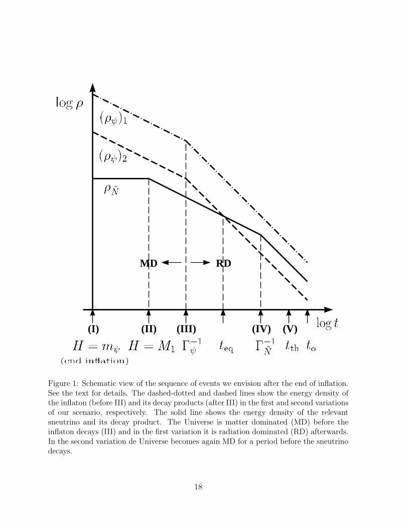
The sequence of events we envision is the following (see Fig.1).

5

I)– The inflaton ψ starts oscillating about the true minimum of its potential when the

expansion rate of the Universe H is HI ≃ mψ. This requirement comes from the solution

of the evolution of a classical field φ in an expanding Universe, φ + 3Hφ+ ∂V/∂φ = 0.

Assuming V (φ) ≃ m2φ2, the solution is oscillatory only for H < m, while for H > m

the solution is overdamped and the field remains stuck at its initial value φ = φo. The

energy in the inflaton oscillations redshifts like matter, so the universe becomes matter

dominated (MD).

II)– Through the same arguments the N1 sneutrino field oscillations start when H =

HII ≃ M1 < HI ≃ mψ. We assume that at this point the inflaton energy density still

dominates, ρψ > ρN .

III)– The 3rd event of our sequence, the decay of the inflaton, happens at a later time

t ≃ Γ−1ψ ≃ M2

P/m3ψ. Using the MD relation between H and t, we obtain that HIII =

(2/3)t−1 ≃ (2/3)Γψ. At this point the Universe becomes radiation dominated (RD) by

the decay products of the inflaton.

IV )– The sneutrino N1 decays later at t ≃ Γ−1N

≃ (h2M1/8π)−1

and using the RD relation

between H and t, HIV = (2t)−1 ≃ h2M1/16π. Here h is the largest h1j coupling. This h

is also the Yukawa coupling constant that dominates the Dirac mass mD1 ≃ hvu. Thus,

using mν1 ≃ h2v2u/M1, we can eliminate the constant h in favor of the lightest neutrino

mass in what follows.

V )–Thermalization happens when the rate of interaction of particles in the Universe,

Γint, becomes equal (and then larger) than the expansion rate of the Universe, i.e. when

H = HV = (2tth)−1 ≃ Γint ≃ nσ, where n is the number density of particles and σ

their typical cross section. The actual lepton asymmetry is either generated or released

when the N1 sneutrino decays. We require to generate in total an asymmetry L > LC ≃

10−2. It is important that the N1 decay occurs before thermalization is achieved. If

so, thermalization happens in the presence of a large lepton asymmetry that breaks the

6

electroweak symmetry from the beginning of the thermal bath and, consequently, the

rate of sphalerons is always suppressed.

Let us examine the conditions for the previous sequence of events to be consistent.

The measured anisotropy of the microwave background radiation requires Hinf to be

1013−1014 GeV in most models (even if it may be lower, such as 1011 GeV, in some) [16].

If the inflaton potential during inflation is just quadratic (such as in chaotic inflation)

then mψ ≃ Hinf/3 at the end of inflation (since H2inf = (8π/3)m2

ψψ2/M2

P and generically

ψ ≃ MP ). However, with more complicated potentials, mψ can be smaller and still we

can assume that the potential at the end of inflation is well approximated by m2ψψ

2. For

example if V (ψ) = λψ4 + m2ψψ

2, and the quartic term dominates during inflation then

λ ≃ 10−13 [16]. Assuming that ψ ≃ MP during inflation and mψ ≃ (10−7 or 10−8)MP ,

the quadratic term in the potential would dominate as soon as ψ became smaller than

MP (by a factor of 3 or 30), at the end of inflation. There are some models in which mψ

is even lower, mψ = 10−9MP [17]. In what follows it will be important to have mψ <∼ 1012

GeV, which is perfectly possible.

Notice that HIII ≡ H(t = Γ−1ψ ) ≃ 6 MeV (mψ/1012 GeV)3 and we will be considering

values of M1 larger than HIII , so that N1 starts oscillating before the inflaton decays

(HII ≃ M1 > HIII). In our scenario N1 decays after the inflaton decays (namely HIV <

HIII) if Γψ/ΓN > 1. This requires

M1 < 1.6 × 108GeV(mψ/1012GeV)3/2

(mν1/10−4eV)1/2. (4)

The thermalization time and temperature, tth and Tth, are obtained by estimating the

number density of particles n and their cross section σ. We take n ≃ Pnψ, where P

is the average number of daughter particles produced in a ψ-decay, and the interaction

cross section to be of electromagnetic order σ ≃ α2/E2. Here E is the characteristic

energy of the particles, that redshifted from a value E = mψ/P at t = Γ−1ψ , thus E =≃

7

(mψ/P )[a(t = Γ−1ψ )/a(tth)]. Moreover, nψ redshifts from a value ρψ/mψ at t = Γ−1

ψ , thus

nψ(tth) = (ρψ(t = Γ−1ψ )/mψ)[a(t = Γ−1

ψ )/a(tth)]3 and ρψ(t = Γ−1

ψ ) is the critical density

at H = 23Γψ, i.e. ρψ(t = Γ−1

ψ ) ≃ Γ2ψM

2P/6π. We obtain tth = (36π2M2

P/α4P 6m3

ψ). The

essential condition tth > Γ−1N

requires (using P = 2)

0.67 × 104GeV(mψ/1012GeV)3/2

(mν1/10−4eV)1/2< M1 . (5)

Notice that Eqs. (4) and (5) leave always an interval of four orders of magnitude for

the allowed values of M1, independently of the values of mψ and mν1 . Computing the

critical density ρth at tth, when H = (2tth)−1 and assuming that all that energy goes into

radiation, ρth = (g∗/3)T 4th, we get the reheating temperature, that is very low

Tth =1

34

α2P 3m3/2ψ

g1/4∗ M

1/2P

= 2.3 × 103GeV(

α

10−2

)2 (P

2

)3 (mψ/1012GeV)3/2

(g∗/102)1/4. (6)

We have not yet computed the asymmetry L. As we will see the requirement of a

large enough L sets a lower bound on No, the initial amplitude of the N1 oscillations. We

will initially consider the case when ρψ > ρN at t = Γ−1N

, which implies that (the decay

product of) the inflaton dominates the energy density at all previous times (see Fig. 1).

This sets an upper bound on No and the viability of this variation of our model depends

on the existence on an allowed interval for No.

Defining ǫ as the net lepton number per N1 particle at decay, the total lepton number

density at t = Γ−1N1

is nL ≃ ǫ nN1(t = Γ−1

N1

) ≃ ǫ ρN(t = Γ−1N

)/M1, where ρN redshifted as

matter from the moment N1 oscillations started, i.e. t = M−11 , when ρN = M2

1 N2o (recall

that we assume the N1 potential is dominated by the quadratic term). Thus,

nL ≃ ǫ M1N2o

[

a(t = M−11 )

a(t = Γ−1N

)

]3

=ǫ N2

o Γ1/2ψ Γ

3/2

N

M1. (7)

In obtaining Eq. (7) it is necessary to remember that the Universe goes from MD to RD

at t = Γ−1ψ , which occurs between t = M−1

1 and t = Γ−1N

. The entropy density at t = Γ−1N

8

is s ≃ 4[

ρψ(Γ−1N

)]3/4

and, since ρψ dominates the energy density of the Universe, we can

equal ρψ to the critical density at the time, i.e. ρψ = (3/8π)M2P (Γ2

N/4). We obtain

L =nLs

≃3.5ǫN2

oΓ1/2ψ

M1 M3/2P

≃3.5ǫN2

om3/2ψ

M1 M5/2P

. (8)

The condition L > LC translates into

No > 0.54 1017GeV(

LC0.1 ǫ

)1/2 (M1/104GeV)1/2

(mψ/1011GeV)3/4. (9)

On the other hand ρψ/ρN ≃ 0.03(MP/No)2(ΓN/Γψ)

1/2 at t = Γ−1N

, and requesting

ρψ/ρN > 1 yields

No < 0.75 × 1017GeV(

mν1/10−4eV)1/4 (M1/104GeV)1/2

(mψ/1011GeV)3/4. (10)

This condition translates into an upper bound on L

L < 0.13 ǫ (mν1/10−4eV)1/2 (11)

thus L > LC only if ǫ > 7LC(10−4 eV /mν1)1/2. If mν1 ≃ 10−4 eV, then ǫ needs to be

near maximum, ǫ >∼ 10−1. Let us see now that these large values of epsilon are easily

obtainable in our scenario.

There are two generic mechanisms to obtain a non-zero ǫ, i.e. a net lepton number

per N decay: one is to generate ǫ during the decay, due to CP and L violation in N decay

modes, starting from an L = 0, N condensate, another is the generation of an L asym-

metric condensate, due to CP and L violating effective operators. In the MSSM model

supplemented with three right-handed neutrinos (Ni, i = 1, 2, 3) the generation of ǫ in

the N decay has been studied in the literature. If M3 = M1, then ǫ ≃ ln(2)Im(h233)/8π

[18] could be as large as 10−2, otherwise there is a suppression factor ≃M1/M3 [19]. Here

h33 is assumed to be the largest hij coupling in Eq. (3), and Im(h233) could be as large

as 1. However, we prefer not to impose any lower bound on the ν3 mass, thus leaving

open the possibility of M3 >> M1.

9

This leaves us only the second method to account for the large ǫ needed. In this case,

the decay of N1, releases the lepton-number asymmetry accumulated in the condensate

due to the appearance of effective lepton number violating soft supersymmetry breaking

terms. These operators are due to the usual mechanism of supersymmetry breaking

in the MSSM, i.e. supergravity breaking in a hidden sector. The main term of this

type in our model is O ≃ m3/2M1N1N1, which yields a lepton number per N1 particle

ǫ = Im(< O >o)(M21 No

2)−1 [7], where < O >o≃ m3/2M1No

2is the initial value of the

L-violating operator, thus, assuming Im(< O >o) ≃< O >o we obtain ǫ ≃ m3/2M−11 .

Replacingm3/2 ≃ 1 TeV, we see that ǫ >∼ 10−1 is possible ifM1 < 10 TeV, which is allowed

by Eq (5), even if mν1 ≃ 10−4 eV (recall that mψ can be as low as 1011 GeV, a possibility

in favor of which we argued above). Actually, the value of ǫ obtained is in general higher

than this estimate because at the beginning of the oscillations the effective value of m3/2

is O(H), rather than O(1 TeV), due to the supersymmetry breaking triggered by the

non-zero vacuum energy (see below). Consequently, < O >o is much larger, an thus the

L generated. Actually, a value ǫ ≃ O(1) may be available, even for M1 < 10 TeV. So,

the previous estimate ǫ ≃ O(1 TeV)M−11 , represents a lower bound on ǫ rather than a

precise value.

We see in Eq. (11) that even with ǫ ≃ 1, L can be up to O(10) LC but not much

larger, unless mν1 > 10−4 eV. We have so far kept mν1 ≃ 10−4 eV because this value can

easily accommodate the MSW solution to the solar neutrino problem. Since the mass

square difference between ν1 and ν2 needs to be ∆m2 ≃ 10−6 eV2 it is enough to choose

mν1 < mν2 ≃ 10−3 eV. However many models including this solution, mainly those trying

to accommodate simultaneously various of the hints for non-zero neutrino masses [20],

propose much larger mν values, such as mν1 ≃ O(eV). In this case the two oscillating

neutrinos are almost degenerate, mν1 ≃ mν2 . This is the scenario we would need to

accept in order to relax numerically the bound from Eq. (10) by one order of magnitude,

10

i.e. for mν1 = 1 eV, keeping M1 and mψ the same, we get from Eq.(10)

No < 0.75 × 1018GeV (mν1/1eV)1/4 (M1/104GeV)1/2

(mψ/1011GeV)3/4. (12)

In this case, from Eq (11) we see that L < 13ǫ with mν1 ≃ 1 eV, so L could easily be up

to 102LC .

We see that the best solutions, those with larger L, tend to saturate the upper bounds

in Eqs.(10) and (11) so that at t = Γ−1N

we have ρN ≃ ρψ. This leads us to the second

variation of our model, namely to relax the condition of ψ-dominance, that yield Eqs.

(10) or (12), and allow ρN to become larger than ρψ in the period, after t = M−11 , in

which ρN behaves like matter (N1 is oscillating) and ρψ (actually the density of their

decay products) behaves like radiation.

Requesting the moment of equality, teq, namely the moment at which ρN (teq) =

ρcritical, to happen before the N decay, that is teq ≃ 0.5(

MP/No

)4Γ−1ψ < Γ−1

N, reverses

the inequality in Eq. (10) (and Eq. (12)), into an upper bound on No

No > 0.75 × 1017GeV(

mν1

10−4eV

)1/4 (M/104GeV)

(mψ/1011GeV)

3/4

. (13)

In this case the s-neutrino decay is responsible for both, the production of the lepton

asymmetry in fermions and the reheating of the Universe. Since nL = ǫρN (t = Γ−1N

)/M1

and s = 4[

ρN (t = Γ−1N

)]3/4

, we obtain

L =nLs

≃ ǫ

4M1

(

ρN (Γ−1N )

)1/4 ≃ 0.1ǫ

√

MPΓN

M1

. (14)

In obtaining this equation we need to notice that, while at the beginning of the N1

oscillations we still have ρN = M2N2o , as before (see Eq. (7)), now in the redshift factor

[

a(t = M−1)/a(t = Γ−1N

)]3

we have to take into account that the Universe is radiation

dominated between t ≃ Γ−1ψ and teq, and matter dominated before and after (until N1

decay), see Fig. 1. Substituting, ΓN ≃ mν1M21 /8πv

2u we get

L = 0.2 ǫ(

mν1

10−4eV

)1/2

. (15)

11

This L is about the maximum allowed in the previous scenario, Eq (11). Eq. (15) shows

that L can be larger for larger values of mν1 . On the other hand, too large values of mν1

may lead to erasure of L. In order to see this point, let us consider the thermalization in

this scenario. Here, the thermalization occurs instantaneously after the N decay, because

the rate of interaction of the decay products Γint = PnNσ = P 3nNα2M−2

1 at the moment

of decay, is larger than the expansion rate of the Universe at that time, H ≃ ΓN ,

ΓintΓN

≃ α2

48π2P 3M

2P

v2u

mν1

M1≃ 2 × 1011

(

α

100

)2 (P

2

)3 ( mν1

10−4eV

)

(

104GeV

M1

)

. (16)

Thus, the N energy density is immediately thermalized after the decay, ρN (Γ−1N

) =

(3/8π)M2PΓ2

N= (g∗/3)T 4

th, and

Tth ≃M1

√

MP mν1

(30π3g∗)1/4vu≃ 5 × 103GeV

(g∗/100)1/4

(

M1

104GeV

)(

mν1

10−4eV

)1/2

. (17)

Notice that Tth < M1 if mν1 < 4 × 10−4 eV, thus the sneutrinos N1 are not present in

the thermal bath. For larger values of mν1 , Tth > M1 and one should worry about the

erasure of L caused by the decay of the N1 present in the thermal bath. Even if the L

initially generated could be as large as 102LC , with mν1 ≃ 1 eV this erasure could lower

L considerably. If we do not want to worry about this source of L-erasure, the value of

mν1 is fixed at mν1 ≃ 10−4 eV, since it cannot be smaller for L >∼ LC , Eq. (15).

Notice that in the first variation of our scenario the preferred neutrino masses are of

order eV or larger. Without any major modification of our model we could choose ν1 to be

heaviest of the three light neutrinos. In this case the lightest right handed neutrino would

mix in the mass matrix preferably with the heaviest light neutrino and not the lightest,

in a see-saw scenario with mDν1

≃ mDν2

≃ mDν3

. Doing so the two lightest neutrino masses

are unconstrained in our model. We could do the same thing in the second variation of

our scenario, but in this case the preferred value of the heaviest neutrino would be 10−4

eV. This would not be compatible with the heaviest neutrino accounting for part of the

dark matter, for example something totally possible in the first variation.

12

Let us address the issue of how the necessary N0 could be generated. We have seen

that in the first scenario we considered that N0 has to be between 1017 and 1018 GeV,

while in the second scenario we need N0 > 1017 GeV. There are several mechanisms

that can produce a value of No ≃ 10−2MP or larger. Let us recall that during inflation

supersymmetry is necessarily broken since the energy density Vo is non zero. This induces

a mass proportional to the Hubble parameter H for all flat directions, thus m2N1

=

c H2 + M2. Dine et al. [21] assumed that c is negative and of order one, and that

non-renormalizable terms δW ≃ λNn1 /(n(βMP )n−3) in the superpotential stabilize the

minimum to the value

No =

(√−c H(βMP )n−3

(n− 1) λ

)1/(n−2)

. (18)

It is obvious that H < No < MP (with the constants β and c of order one) and No

becomes arbitrarily closer to βMP for large n. The conditions to obtain the necessary

negative effective masses and non-renormalizable terms to lift the “flat” direction of the

potential in supergravity scenarios have in general been examined in Ref. [22], both

in D- and F- inflationary models. Large negative masses square favour F-inflationary

scenarios in which the Kahler potential contains a large mixing of the sneutrino and

the inflaton in the term quadratic in N1. This is a strong constraint on supergravity

scenarios, which, for example, excludes minimal supergravity and in string-based models

requires that the inflaton be a T modulus field (and not the dilaton S). In particular, in

orbifold constructions, m2N1

≤ 0 at the origin, is obtained if the modular weight of the

N1 field is nN1≤ −3.

There is another possibility we think cannot be neglected, namely that c is very small.

The value m2N1

≃ 0 at the origin can also appear in a natural way, with no fine-tuning

at all, both in F -inflation and in D-inflationary scenarios [22]. In this case, No departs

from zero due to quantum fluctuations during the Sitter phase. The coherence length of

13

these fluctuations ℓcoh ≃ H−1inf exp(3H2

inf/2m2) ≃ H−1

inf exp(3/2c) would be large enough

to encompass our present visible Universe if c < 2 × 10−2. When the coherence length

is much larger than the horizon, ℓcoh ≫ H−1inf , as is the case here, the field N1 can be

treated as classical and

No =√

〈N21 〉 ≃

√

3

8π2

H2inf

M=

√

3

8π2

Hinf√c. (19)

For No ≃ 1017 GeV and Hinf ≃ 1013 GeV we need c ≃ 4 × 10−10. This small value of

c can be naturally achieved in string-based F -inflationary models. In T -driven models

with orbifold compactifications this possibility is insured by the discrete character of the

modular weights, since it is enough that nN1= −3. In D-inflationary models, usually

the D-term is associated to an anomalous U(1), and m2N1

≃ 0 results if the N1 field is a

singlet under that group [22].

In conclusion, we presented here a model to produce a very large lepton asymmetry

L ≃ 10−2 − 1 without producing a large baryon asymmetry. The model is based on

the Affleck and Dyne scenario, in which the field acquiring a large vacuum expectation

value during inflation is an sneutrino right. We take as a specific model the MSSM sup-

plemented with three right handed neutrino singlet superfields, besides an inflationary

sector. We considered two variations of one scenario, one in which the inflaton energy

dominates at reheating and another in which the sneutrino energy dominates then. In

both cases we required L to be large enough for the electroweak symmetry to be spon-

taneously broken at all temperatures after inflation, with the consequent suppression of

sphaleron transitions. In order to obtain this, in our scenario the large L is generated

before thermalization. The models considered are realistic. The first variation works

better if the lightest neutrino mass is of O(1 eV). In this case the MSW solution to the

solar neutrino problem would require almost degenerate neutrinos, as proposed in models

trying to account simultaneously for several of the present hints for non-zero neutrinos

14

masses. Alternatively, if the bounds apply to the heaviest neutrino instead, the lighter

neutrino masses are unconstrained. The second variation works better when the lightest

neutrino mass is of O(10−4) eV, what can easily accommodate the masses needed for the

MSW mechanism. In both cases the preferred value of the lightest right handed neutrino

is of O(TeV) and the vacuum expectation value of the s-neutrino field during inflation

must be larger than 1017 GeV. We also commented on ways to obtain naturally these

large values for the sneutrino condensate. We have not addressed here how the baryon

asymmetry could be generated. A very interesting possibility that deserved further study

is that the out of equilibrium sphaleron transitions may translate a minor part of the L

asymmetry into B [10].

Acknowledgements

We thank the Aspen Center for Physics, where this paper was initiated, for its hospitality.

References

[1] R. V. Wagoner, W. A. Fowler and F. Hoyle, Ap. J. 148 (1967) 3; A. Yahil and G.

Beaudet, Ap. J. 206 (1976) 26; Y. David and H. Reeves, Physical Cosmology (ed.

R. Balian, J. Audouze and D. N. Schramm, North-Holland, Amsterdam, 1980); J.

N. Fry and C. J. Hogan, Phys. Rev. Lett. 49 (1982) 1783; R. J. Scherrer, Mon.

Not. Roy. Astron. Soc. 205 683; N. Terazawa and K. Sato, Ap. J. 294 (1985) 9; K.

Olive, D. N. Schramm, D. Thomas and T. Walker, Phys. Lett. B265 (1991) 239; G.

Starkman Phys. Rev. D45 (1992) 476.

[2] H. Kang and G. Steigman, Nucl. Phys. B372 (1992) 494.

[3] K. Freese, E. W. Kolb and M. S. Turner, Phys. Rev. D27 (1983) 1689.

15

[4] M. White, J. Navarro, A. Evrard and C. Frenk, Nature 366 (1993) 429.

[5] G Steigman and J. Felten, OSU-TA-24-94, astro-ph/9502029.

[6] J. A. Harvey and E. W. Kolb, Phys. Rev. D24 (1981) 2090.

[7] I. Affleck and M. Dine, Nucl. Phys. B249 (1985) 361.

[8] P. Langacker, G. Segre and S. Soni, Phys. Rev. D26 (1982) 3425.

[9] V. A. Kuzmin, V. A. Rubakov and M. E. Shaposnikov, Phys. Lett. B155 (1985) 36.

[10] J. Liu and G. Segre, Phys. Lett. B338 (1994) 259.

[11] A. D. Dolgov and D. P. Kirilova, J. Moscow Phys. Soc. 1 (1991) 217 (see also A.

D. Dolgov, IUPAP Conference on Primordial Nucleosynthesis and Evolution in the

Early Universe, Tokyo, 1990); A. D. Dolgov, Phys. Rep. 222 (1992) 309.

[12] R. Foot, M. J. Thompson and R. R. Volkas, Phys. Rev D53 (1996) 5349; X. Shi,

Phys. Rev. D54 (1996) 2753.

[13] A. D. Linde, Phys. Rev. D14 (1976) 3345.

[14] S. Davidson, H. Murayama and K. Olive, Phys. Lett. B328 (1994) 345.

[15] L. Kofman, A. D. Linde and A. A. Starobinsky, Phys. Rev. Lett. 73 (1994) 3195;

Phys. Rev. Lett. 76 (1996) 1011.

[16] D. S. Salopek, Phys. Rev. Lett. 69 (1992) 3602; L. Krauss and M. White, Phys.

Rev. Lett. 69 (1992) 869; A. Liddle and D. Lyth, Phys. Rep. 231 (1993) 1.

[17] G. G. Ross and S. Sarkar, Nucl. Phys. B461 (1996) 597.

16

[18] H. Murayama, H. Suzuki, T. Yanagida and J. Yokoyama, Phys. Rev. Lett. 70 (1993)

1012.

[19] B. Campbell, S. Davidson and K. Olive, Nucl. Phys. B399 (1993) 111.

[20] D. Caldwell and R. Mohapatra, Phys. Rev. D48 (1993) 3259; J. T. Peltoniemi and

J. W. F. Valle, Nucl. Phys. B406 (1993) 409.

[21] M. Dine, L. Randall and S. Thomas, Nucl. Phys. B458 (1996) 291.

[22] J. A. Casas and G. B. Gelmini, Phys. Lett. B410 (1997) 36.

17

log

log tMD RD

(I) (II) (III) (V)(IV)H =M1 1 teq 1~N tth toH = m

( )1( )2 ~N

(end in ation)Figure 1: Schematic view of the sequence of events we envision after the end of inflation.See the text for details. The dashed-dotted and dashed lines show the energy density ofthe inflaton (before III) and its decay products (after III) in the first and second variationsof our scenario, respectively. The solid line shows the energy density of the relevantsneutrino and its decay product. The Universe is matter dominated (MD) before theinflaton decays (III) and in the first variation it is radiation dominated (RD) afterwards.In the second variation de Universe becomes again MD for a period before the sneutrinodecays.

18