Generating virtual microphone signals using geometrical information gathered by distributed arrays

GENERATING VIRTUAL MICROPHONE SIGNALS USING GEOMETRICALINFORMATION GATHERED BY DISTRIBUTED ARRAYS

Giovanni Del Galdo1, Oliver Thiergart2, Tobias Weller1, and Emanuel A.P. Habets2

1Fraunhofer Institute for Integrated Circuits IIS, Erlangen, Germany2International Audio Laboratories Erlangen, Germany

Email: [email protected]

ABSTRACT

Conventional recording techniques for spatial audio are limited tothe fact that the spatial image obtained is always relative to the po-sition in which the microphones have been physically placed. Inmany applications, however, it is desired to place the microphonesoutside the sound scene and yet be able to capture the sound from anarbitrary perspective. This contribution proposes a method to placea virtual microphone at an arbitrary point in space, by computing asignal perceptually similar to the one which would have been pickedup if the microphone had been physically placed in the sound scene.The method relies on a parametric model of the sound field basedon point-like isotropic sound sources. The required geometrical in-formation is gathered by two or more distributed microphone arrays.Measurement results demonstrate the applicability of the proposedmethod and reveal its limitations.

Index Terms— Spatial sound, Sound localization, Audiorecording, Parameter estimation

1. INTRODUCTION

Spatial sound acquisition aims at capturing either an entire soundscene or just certain desired components, depending on the applica-tion at hand. Several recording techniques providing different advan-tages and drawbacks are available for these purposes. For instance,close talking microphones are often used for recording individualsound sources with high SNR and low reverberation, while moredistant configurations such as XY stereophony represent a way forcapturing the spatial image of an entire sound scene. More flexibilityin terms of directivity can be achieved with beamforming, where amicrophone array can be used to realize steerable pick-up patterns.Even more flexibility is provided by parametric methods, such asdirectional audio coding (DirAC) [1], in which it is possible to real-ize spatial filters with arbitrary pick-up patterns [2] as well as othersignal processing manipulations of the sound scene [3, 4].

All these methods have in common that they are limited to a rep-resentation of the sound field with respect to only one point, namelythe measurement location. Thus, the required microphones must beplaced at very specific, carefully selected positions, e. g., close tothe sources or such that the spatial image can be captured optimally.In many applications however, this is not feasible and therefore itwould be beneficial to place several microphones further away fromthe sound sources and still be able to capture the sound as desired.

There exist several field reconstruction methods for estimatingthe sound field in a point in space other than where it was measured.One method is acoustic holography [5], which allows to computethe sound field at any point within an arbitrary volume given that the

sound pressure and particle velocity is known on its entire surface.Therefore, when the volume is large, an unpractically large num-ber of sensors is required. Moreover, the method assumes that nosound sources are present inside the volume, making the algorithmunfeasible for our needs. The related wave field extrapolation [5]aims at extrapolating the known sound field on the surface of a vol-ume to outer regions. The extrapolation accuracy however degradesrapidly for larger extrapolation distances as well as for extrapola-tions towards directions orthogonal to the direction of propagationof the sound [6]. In [7] a plane wave model is assumed, such thatthe field extrapolation is possible only in points far from the actualsound sources, i. e., close to the measurement point.

To overcome the drawbacks of these field reconstructing meth-ods, this contribution proposes a parametric method capable of es-timating the sound signal of a virtual microphone placed at an arbi-trary location. In contrast to the methods previously described, theproposed method does not aim directly at reconstructing the soundfield, but rather at providing sound that is perceptually similar to theone which would be picked up by a microphone physically placedat this location. This is possible thanks to a parametric model ofthe sound field based on isotropic point-like sound sources (IPLS).The required geometrical information, namely the instantaneous po-sition of all IPLS, is gathered via triangulation of the directions ofarrival (DOA) estimated with two or more distributed microphone ar-rays. Therefore, knowledge on the relative position and orientationof the arrays is required. Notwithstanding, no a priori knowledgeon the number and position of the actual sound sources is neces-sary. Given the parametric nature of the method, the virtual micro-phone can possess an arbitrary directivity pattern as well as physicalor non-physical behaviors, e. g., with respect to the pressure decaywith distance. The presented approach is verified by studying the pa-rameter estimation accuracy based on measurements in a reverberantenvironment.

The paper is structured as follows: In Section 2 the sound fieldmodel is introduced and the geometric parameter estimation algo-rithm is derived. In Section 3 the virtual microphone approach ispresented and discussed in detail. The algorithm is verified withmeasurement results in Section 4. Section 5 concludes the paper.

2. GEOMETRIC PARAMETER ESTIMATION

2.1. Sound Field Model

The sound field is analyzed in the time-frequency domain, for in-stance obtained via a short-time Fourier transform (STFT), in whichk and n denote the frequency and time indices, respectively. Thecomplex pressure Pv(k, n) at an arbitrary position pv for a certain

2011 Joint Workshop on Hands-free Speech Communication and Microphone Arrays May 30 - June 1, 2011

978-1-4577-0999-9/11/$26.00 ©2011 IEEE 185

!1

!2

O

pIPLS(k, n)

x

y

p1

p2

e1

e2

d2

d1

s

c1

pv

c2

Fig. 1. Geometry used throughout this contribution

k and n is modeled as a single spherical wave emitted by a narrow-band isotropic point-like source (IPLS), i. e.,

Pv(k, n) = PIPLS(k, n) · "`

k, pIPLS(k, n), pv

´

, (1)

where PIPLS(k, n) is the signal emitted by the IPLS at its posi-tion pIPLS(k, n). The complex factor " (k, pIPLS, pv ) expressesthe propagation from pIPLS(k, n) to pv , i. e., it introduces appro-priate phase and magnitude modifications as discussed in Section 3.Hence, we assume that in each time-frequency bin only one IPLScan be active. Nevertheless, multiple narrowband IPLSs located atdifferent positions can be active at a single time instance n.

Each IPLS models either direct sound or a distinct room reflec-tion, such that its position pIPLS(k, n) ideally corresponds to an ac-tual sound source located inside the room, or a mirror image soundsource located outside, respectively. Notice that this single-wavemodel is accurate only for mildly reverberant environments giventhat the source signals fulfill the W -disjoint orthogonality (WDO)condition, i. e., the time-frequency overlap is sufficiently small. Thisis normally true with speech signals [8].

The next two sections deal with the estimation of the posi-tions pIPLS(k, n) whereas Section 3 deals with the estimation ofPIPLS(k, n) and the computation of " (k, pIPLS, pv ).

2.2. Position Estimation

The position pIPLS(k, n) of an IPLS active in a certain time-frequency bin is estimated via triangulation on the basis of thedirection of arrival (DOA) of sound measured in at least two differ-ent observation points.

Let us consider the geometry in Fig. 1 where the IPLS of thecurrent (k, n) is located in the (unknown) position pIPLS(k, n). Inorder to determine the required DOA information, we use two micro-phone arrays with known geometry, position, and orientation placedin p1 and p2, respectively. The array orientations are defined bythe unit vectors c1 and c2. The DOA of the sound is determined inp1 and p2 for each (k, n) using a DOA estimation algorithm, forinstance as provided by the DirAC analysis [1]. The output of theDOA estimators from the point of view (POV) of the arrays can beexpressed as the unit vectors ePOV1 (k, n) and ePOV

2 (k, n) (not de-picted in the plot). For instance, when operating in 2D,

ePOV1 (k, n) =

»

cos(!1(k, n))sin(!1(k, n))

–

, (2)

where!1(k, n) is the azimuth of the DOA estimated at the first array,as depicted in Fig. 1. The corresponding DOA unit vectors e1(k, n)

and e2(k, n), with respect to the global coordinate system in theorigin O, are computed via

e1(k, n) = R1 · ePOV1 (k, n),

e2(k, n) = R2 · ePOV2 (k, n),

(3)

whereR are coordinate transformation matrices, e. g.,

R1 =

»

c1,x !c1,y

c1,y c1,x

–

, (4)

when operating in 2D and c1 = [c1,x, c1,y ]T. For carrying out thetriangulation we define the direction vectors d1(k, n) and d2(k, n)as

d1(k, n) = d1(k, n) e1(k, n),

d2(k, n) = d2(k, n) e2(k, n),(5)

where d1(k, n) = ||d1(k, n)|| and d2(k, n) = ||d2(k, n)|| are theunknown distances between the IPLS and the two microphone ar-rays. The triangulation is computed by solving

p1 + d1(k, n) = p2 + d2(k, n) (6)

for either d1(k, n) or d2(k, n). Finally, the position pIPLS(k, n) ofthe IPLS is given by

pIPLS(k, n) = d1(k, n)e1(k, n) + p1. (7)

Equation (6) always provides a solution when operating in 2D,unless e1(k, n) and e2(k, n) are parallel. When using more then twomicrophone arrays or when operating in 3D, however, triangulationis not directly possible when the direction vectors d do not intersect.In this case, we can compute the point which is closest to all directionvectors d and use the result as position of the IPLS.

Notice that in general all observation points p1, p2, . . . mustbe located such that the sound emitted by the IPLS falls into thesame temporal block n. Otherwise, combining the DOA informa-tion for a certain time-frequency bin cannot provide useful results.This requirement is fulfilled when the distance ! between any twoobservation points is smaller than

!max = cnFFT(1 ! R)

fs

, (8)

where nFFT is the STFT window length, 0 " R < 1 specifiesthe overlap between successive time frames, and fs is the samplingfrequency. For example, for a 1024-point STFT at 48 kHz with 50%overlap (R = 0.5), the maximum spacing between the arrays tofulfill the above requirement is! = 3.65 m.

2.3. Parameter Estimation in Practice

When only direct sound and distinct room reflections are present,the estimator introduced in the previous section leads to a positionpIPLS(k, n), which corresponds to either an actual sound source (fordirect sound) or an image mirror source (for a distinct room reflec-tion). However, in most cases, the sound field measured in a roomdoes not consist only of direct sound and distinct room reflections,i. e., non-diffuse sound, but also of diffuse sound, which is not con-sidered in the model in (1).

In the case of pure diffuse sound, the estimated positionpIPLS(k, n) is random and its distribution depends on the DOAestimator used. For instance, when using DirAC [1] the estimatedDOA is a uniformly distributed random variable. In this case, the

186

−2 −1 0 1 20

0.5

1

1.5

2

20

30

40

50

60

x [m]

y[m]

Fig. 2. Black lines: equally spaced DOA vectors from the point ofview of two arrays. Greyscale plot: PDF in dB of the localized posi-tion when both arrays estimate uniformly distributed random DOAs.

triangulation in (6) leads to positions which are concentrated aroundthe observation points p1 and p2. To visualize this, please considerFig. 2, which shows two array positions at p1 = [!1, 0]T andp2 = [1, 0]T and several local DOA vectors e1 and e2 (representedby the black lines) equally spaced in azimuth. It can be seen thatthe intersection points are more dense for distances closer to the mi-crophone arrays, and less dense for larger distances. This confirmsthat when both arrays estimate uniformly distributed random DOAs,the triangulation yields positions with higher probability near thetwo arrays. This is also shown by the greyscale plot in Fig. 2 whichdepicts the probably density function (PDF) (in dB) of the localizedposition when both arrays estimate uniformly distributed randomDOAs.

The two specific scenarios discussed above, namely non-diffusesound only and diffuse sound only, accurately describe most scenar-ios encountered in practice in case of speech signals. In fact, thefrequent onsets and speech pauses lead to situations in which eithernon-diffuse sound or diffuse sound is dominant.

3. VIRTUALMICROPHONE GENERATION

Once the IPLS have been localized as discussed in the previoussection, the omnidirectional pressure signal Pv (k, n) at the (arbi-trary) position pv of the virtual microphone can be estimated follow-ing (1). Based on this signal we can then derive the output Pv (k, n)of a virtual microphone with arbitrary directivity. The pressure sig-nal PIPLS(k, n) required in (1) is obtained from the pressure signalPref(k, n) of a physical reference microphone located in pref . Anal-ogously to (1), we can write

Pref(k, n) = PIPLS(k, n) · " (k, pIPLS, pref) , (9)

which is solved for PIPLS(k, n). The reference signal Pref(k, n)can be obtained for instance from one microphone of the arrays, asdiscussed in Section 3.1.

In general, the complex factor " (k, pa, pb) expresses the phaserotation and amplitude decay introduced by the propagation of aspherical wave from its origin in pa to pb. However, practical testsindicated that considering only the amplitude decay in " leads toplausible impressions of the virtual microphone signal with signif-icantly fewer artifacts compared to also considering the phase rota-tion. The exact computation of the reference signal Pref(k, n), thepropagation factor ", and the virtual microphone output Pv (k, n) isgiven in the following sections.

3.1. Reference Pressure Signal

The reference pressure signal Pref(k, n) is derived from the arraymicrophones. Assuming that the microphone arrays consist of om-nidirectional sensors, there exist different approaches to generatePref(k, n), for instance

• using one specific, fixed microphone,

• using the microphone which is closest to the localized IPLSor to the position of the virtual microphone,

• combining the microphone signals of one array,

• combining all available microphones.

Using the array microphone closest to the position pIPLS(k, n) ofthe IPLS potentially provides higher SNR and lower reverberation(since the distance to the sound source is smaller), but will likelyintroduce coloration or artifacts when switching for each (k, n) toa different sensor. A similar observation can be made when com-bining the array sensors, e. g., via beamforming. A beamformer canbe realized in a straightforward manner by exploiting the geometri-cal information on the IPLS. For instance, one possible beamform-ing solution combining both microphone arrays can be realized bycompensating the delay between all sensor signals and then com-puting the sum. Since both arrays are sufficiently close such that asound event appears for all microphones in the same time frequencybin (k, n), the delay compensation can be realized by phase rota-tion of each (k, n). This requires exact knowledge of the phase dif-ferences between the sensors, which can be directly obtained fromthe geometrical parameters, namely from the distances between theindividual sensors and the position of the current IPLS. This ap-proach however requires a very precise parameter estimation, espe-cially when compensating the delays between the sensors of differentarrays. The performance of the different methods for computing thereference pressure signal is topic of current research. For this con-tribution, we restrict the discussion to the case in which we take asreference pressure signal Pref(k, n) the array microphone which isclosest to the virtual microphone in pv , as this requires the smallestmodifications for generating the virtual microphone signal and thus,potentially provides the fewest artifacts.

3.2. Magnitude Reconstruction

The sound energy which can be measured in a certain point in spacedepends strongly on the distance r from the sound source. In manysituations, this behavior can be modeled with sufficient accuracyusing well-known physical principles, such as the 1/r decay of thesound pressure in the far-field of a point source. Therefore, whenthe distance of both the reference microphone and the virtual micro-phone from the sound source is known, we can estimate the soundenergy at the position of the virtual microphone from the signal en-ergy of the reference microphone. This means that the output signalof the virtual microphone can be obtained by applying proper gainsto the reference pressure signal.

Let the reference microphone be located in pref = p1 as shownin Fig. 1 and the virtual microphone be located in pv . Since thegeometry in Fig. 1 is known in detail, we can easily determine thedistance d1(k, n) = ||d1(k, n)|| between the reference microphoneand the IPLS, as well as the distance s(k, n) = ||s(k, n)|| betweenthe virtual microphone and the IPLS, namely

s(k, n) = ||s(k, n)|| = ||p1 + d1(k, n) ! pv ||. (10)

187

A

O

r = 2m

p2

B

p1

P1

P2

P3

P4

d = 3.2cm

Fig. 3. Left: measurement setup with two sourcesA and B, and twoarray positions p1 and p2. Right: microphone array consisting offour omnidirectional sensors.

The sound pressure Pv(k, n) at the position of the virtual micro-phone is computed by combining (1) and (9), leading to

Pv (k, n) =" (k, pIPLS, pv )" (k, pIPLS, pref)

Pref(k, n). (11)

As mentioned at the beginning of the section, the factors " only con-sider the amplitude decay due to the propagation. Assuming for in-stance that the sound pressure decreases with 1/r, then

Pv(k, n) =d1(k, n)s(k, n)

Pref(k, n). (12)

When the model in (1) holds, i. e., when only direct sound is present,then (12) can accurately reconstruct the magnitude information.However, in case of pure diffuse sound fields, i. e., when the modelassumptions are not met, the presented method yields an implicitdereverberation of the signal when moving the virtual microphoneaway from the positions of the sensor arrays. In fact, as discussedin Section 2.3, in diffuse sound fields we expect that most IPLS arelocalized near the two sensor arrays. Thus, when moving the virtualmicrophone away from these positions, we likely increase the dis-tance s = ||s|| in Fig. 1. Therefore, the magnitude of the referencepressure is decreased when applying a weighting according to (11).Correspondingly, when moving the virtual microphone close to anactual sound source, the time-frequency bins corresponding to thedirect sound will be amplified such that the overall audio signal willbe perceived less diffuse. By adjusting the rule in (12), one cancontrol the direct sound amplification and diffuse sound suppressionat will.

3.3. Virtual Microphone Directivity

From the geometrical information estimated in Section 2.2, we canapply arbitrary directivity patterns to the virtual microphone. In do-ing so, one can for instance separate a source from a complex soundscene, assuming that the model assumptions hold.

Since the DOA of the sound can be computed in the position pv

of the virtual microphone, namely

!v(k, n) = arccos

„

s · cv

||s||

«

, (13)

where cv is a unit vector describing the orientation of the virtualmicrophone, we can realize arbitrary directivities for the virtual mi-crophone. For instance,

Pv (k, n) = Pv (k, n)ˆ

1 + cos`

!v (k, n)´˜

(14)

0 5 10 15 20 25 30 35 40

t [ms]

h1(t

)

early partdirect part

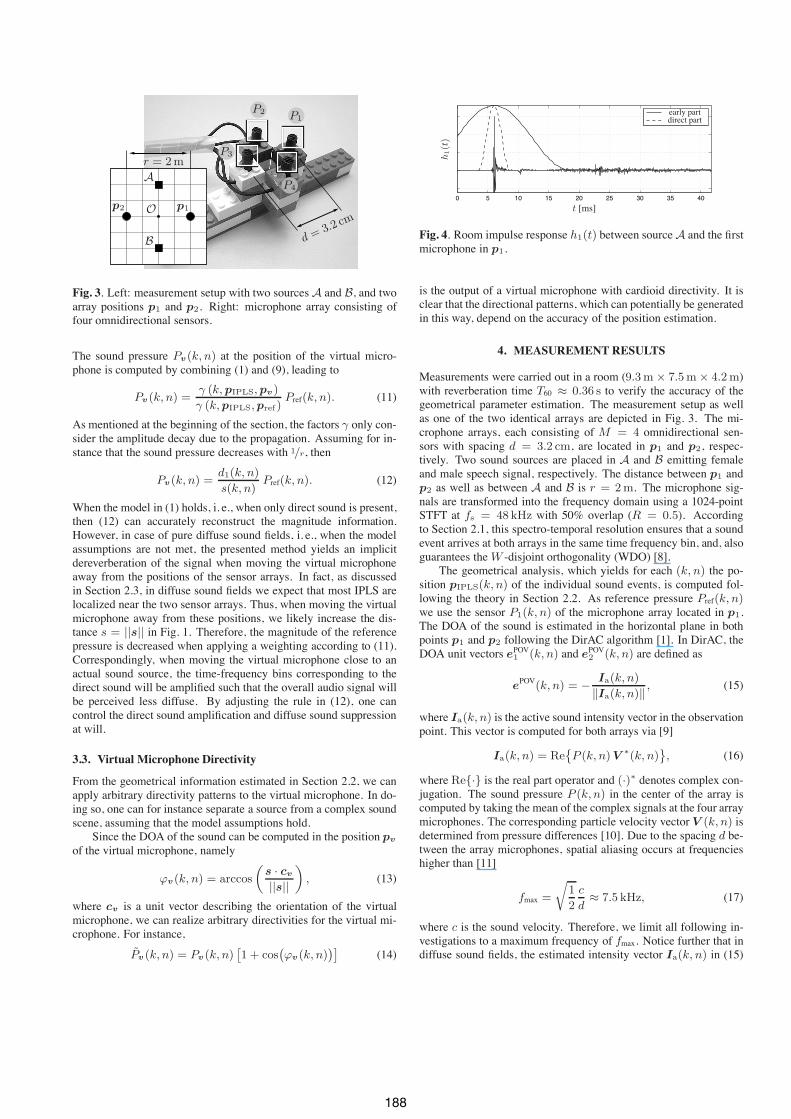
Fig. 4. Room impulse response h1(t) between sourceA and the firstmicrophone in p1.

is the output of a virtual microphone with cardioid directivity. It isclear that the directional patterns, which can potentially be generatedin this way, depend on the accuracy of the position estimation.

4. MEASUREMENT RESULTS

Measurements were carried out in a room (9.3 m # 7.5 m # 4.2 m)with reverberation time T60 $ 0.36 s to verify the accuracy of thegeometrical parameter estimation. The measurement setup as wellas one of the two identical arrays are depicted in Fig. 3. The mi-crophone arrays, each consisting of M = 4 omnidirectional sen-sors with spacing d = 3.2 cm, are located in p1 and p2, respec-tively. Two sound sources are placed in A and B emitting femaleand male speech signal, respectively. The distance between p1 andp2 as well as between A and B is r = 2 m. The microphone sig-nals are transformed into the frequency domain using a 1024-pointSTFT at fs = 48kHz with 50% overlap (R = 0.5). Accordingto Section 2.1, this spectro-temporal resolution ensures that a soundevent arrives at both arrays in the same time frequency bin, and, alsoguarantees theW -disjoint orthogonality (WDO) [8].

The geometrical analysis, which yields for each (k, n) the po-sition pIPLS(k, n) of the individual sound events, is computed fol-lowing the theory in Section 2.2. As reference pressure Pref(k, n)we use the sensor P1(k, n) of the microphone array located in p1.The DOA of the sound is estimated in the horizontal plane in bothpoints p1 and p2 following the DirAC algorithm [1]. In DirAC, theDOA unit vectors ePOV1 (k, n) and ePOV2 (k, n) are defined as

ePOV(k, n) = !

Ia(k, n)%Ia(k, n)%

, (15)

where Ia(k, n) is the active sound intensity vector in the observationpoint. This vector is computed for both arrays via [9]

Ia(k, n) = Re˘

P (k, n) V !(k, n)¯

, (16)

where Re{·} is the real part operator and (·)! denotes complex con-jugation. The sound pressure P (k, n) in the center of the array iscomputed by taking the mean of the complex signals at the four arraymicrophones. The corresponding particle velocity vector V (k, n) isdetermined from pressure differences [10]. Due to the spacing d be-tween the array microphones, spatial aliasing occurs at frequencieshigher than [11]

fmax =

r

12

cd$ 7.5 kHz, (17)

where c is the sound velocity. Therefore, we limit all following in-vestigations to a maximum frequency of fmax. Notice further that indiffuse sound fields, the estimated intensity vector Ia(k, n) in (15)

188

−5 −2.5 0 2.5 5−4

−3

−2

−1

0

1

2

3

4

−50

−40

−30

−20

−10

0

x [m]

y[m]

(a) complete RIR

(b) direct sound

(c) early part

(d) late part

Fig. 5. Spatial power densities (SPD) [dB] of the localized positionspIPLS for a single sound source situation.

points to random directions. Therefore, the directions of the DOAunit vectors ePOV(k, n) are uniformly distributed in 2#, leading tothe distribution in Fig. 2 as discussed in Section 2.3.

4.1. Single Talker Situation

Let us first study the performance of the proposed system for a singletalker situation where only the sound source A is active. Figure 4shows the room impulse response (RIR) h1(t) of sensor P1(k, n)of the microphone array in p1. The direct sound part and the earlypart of the RIR are marked by the two windows. In the followingwe filter out different parts of the measured RIRs by means of thedepicted windows, and then use the resulting impulse responses toconvolve the dry speech signal to obtain the microphone recordings.In doing so, we can analyze separately the influence of the differentparts of the sound field on the parameter estimation.

To investigate the accuracy of the parameter estimation, we com-pute the spatial power density (SPD)"(p) of the estimated IPLS po-sitions pIPLS. The SPD describes the sound energy localized in acertain position p = [x, y]T i. e.,

"(p) =X

K

|Pref(k, n)|2 , (18)

where K =˘

(k, n)|p = pIPLS

¯

and Pref(k, n) is the referencepressure signal as explained in Section 3.1. Before computing "(p),all localized positions pIPLS with distance larger then the room sizeare clipped to the room borders.

The SPDs "(p) for the single source scenario are depicted inFig. 5. Plot (a) shows the results when the complete measured RIRsis used. The white dot represents the true source position while the

−5 −2.5 0 2.5 5−4

−3

−2

−1

0

1

2

3

4

−50

−40

−30

−20

−10

0

x [m]

y[m]

Fig. 6. SPD [dB] of the localized positions pIPLS when both soundsources (marked by the white dots) are active at the same time.

black dots show the microphone arrays. The cross marks the centerof gravity. As can be seen, most energy is localized around the truesource position. However, we notice an estimation bias towards theright array. The energy of the mirror image sources, which ismappedto the room borders, is also clearly visible in the plot. We further no-tice that some energy is distributed around both arrays. This energymainly corresponds to the diffuse sound energy, which, as discussedin Section 2.3, is localized with higher probability around the arraylocations.

To verify this claim, Fig. 5(b)–(d) shows the correspondingSPDs when filtering out different parts of the measured RIRs. No-tice that we use the same decibel scale as in Fig. 5(a), but normalizethe plots to a maximum of 0 dB. When only direct sound compo-nents are present (Fig. 5(b)), nearly all energy is localized aroundthe true source position. In Fig. 5(c), which illustrates the resultwhen only the early part of the sound arrives at the array, we againnotice the localization bias towards the right microphone array. Thisindicates that the ground reflection has a significant influence on theposition estimation. Figure 5(c) depicts the results when only thelate part of the sound arrives at the microphone arrays. In this casemost energy is localized around the array positions, verifying thetheory in Section 2.3.

4.2. Double Talk Situation

For a situation with two speakers active at the same time, the SPDis shown in Fig. 6. The black circles indicate the positions of themicrophone arrays and the white circles indicate the exact speakerpositions. Although both speakers are active at the same time, a dis-tinct power concentration around both true positions of the speakerscan be seen. As for the single talker case, a concentration of energycan be observed around the microphone arrays due to the diffuseenergy in the late signal part (see Fig. 5).

As an example, we place a virtual microphone in the origin. Thesignal from the first microphone of the first array is chosen as thereference signal. Then, this signal is weighted as in (12). To avoidextreme amplifications, the value of ratio of distances has been lim-ited to a reasonable maximum. The spectrogram of the virtual mi-crophone signal Pv(k, n) is shown in Fig. 7(a). In this scenario, firstonly speaker A is active, then only speaker B, and in the end, bothspeakers are active at the same time.

189

10 15 20 25 30 35 40 450

500

1000

1500

2000

2500

3000

3500

4000

−60

−50

−40

−30

−20

−10

0

t [s]

f[Hz]

source A source B A+B

|Pv (k, n)|2 [dB]

(a) virtual omnidirectional sensor

10 15 20 25 30 35 40 450

500

1000

1500

2000

2500

3000

3500

4000

−60

−50

−40

−30

−20

−10

0

t [s]

f[Hz]

source A source B A+B

|Pv (k, n)|2 [dB]

(b) virtual cardioid sensor

Fig. 7. Plot (a) shows the virtual microphone signal Pv (k, n). Plot(b) shows the virtual microphone signal Pv (k, n) when applying acardioid directivity. The virtual microphone is placed in the origindirected towards sourceA.

Since the two sound sources are spatially separated, it is alsopossible to separate their signals by means of a directive virtual mi-crophone. Therefore, in addition to the distance dependent filter acardioid-like pick-up pattern as described in (14) is assigned to thevirtual microphone, with the look direction pointed at speaker A.The spectrogram of the resulting signal (given the same speaker sce-nario as above) is depicted in Fig. 7(b). It can be seen that while thesignal of speaker A remains unchanged, the signal of speaker B ishighly attenuated. The results show that for the presented scenariosource separation is indeed possible to a certain extent using a virtualmicrophone. Nevertheless, appropriate listening tests are necessaryin order to determine quantitatively the signal quality.

5. CONCLUSIONS

This contribution proposes the use of isotropic point-like sources(IPLS) to model a complex sound scene. Each IPLS represents ei-ther direct sound or a distinct room reflection and is active only in asingle time-frequency bin. By estimating the direction of arrival ofsound at two or more points in space, e. g., via microphone arrays,

it is possible to localize the position (direction and distance) of theIPLS. Given the estimated source positions and the pressure signalmeasured at an appropriate reference position, one can compute theoutput signal of an arbitrary virtual microphone. Informal listeningtests indicated that the signal of the virtual microphone is percep-tually similar to the one which would have been measured had themicrophone been placed physically in the sound scene. The paramet-ric nature of the scheme allows us to define an arbitrary directivitypattern for the virtual microphone and also to realize a non-physicalbehavior, for instance by applying an arbitrary decay with distance.The introduced signal model is valid for mildly reverberant environ-ments given that the time-frequency overlap of the emitted soundsource signals is sufficiently small. This assumption is normally truewith speech signals. The proposed approach has been verified bymeasurements in a reverberant environment in both a single and adouble talker scenario.

6. REFERENCES

[1] V. Pulkki, “Spatial sound reproduction with directional audiocoding,” J. Audio Eng. Soc, vol. 55, no. 6, pp. 503–516, June2007.

[2] M. Kallinger, H. Ochsenfeld, G. Del Galdo, F. Kuech,D. Mahne, R. Schultz-Amling, and O. Thiergart, “A spatialfiltering approach for directional audio coding,” in Audio Engi-neering Society Convention 126, Munich, Germany, May 2009.

[3] R. Schultz-Amling, F. Kuech, O. Thiergart, and M. Kallinger,“Acoustical zooming based on a parametric sound field rep-resentation,” in Audio Engineering Society Convention 128,London UK, May 2010.

[4] J. Herre, C. Falch, D. Mahne, G. Del Galdo, M. Kallinger, andO. Thiergart, “Interactive teleconferencing combining spatialaudio object coding and DirAC technology,” in Audio Engi-neering Society Convention 128, London UK, May 2010.

[5] E. G. Williams, Fourier Acoustics: Sound Radiation andNearfield Acoustical Holography, Academic Press, 1999.

[6] A. Kuntz and R. Rabenstein, “Limitations in the extrapolationof wave fields from circular measurements,” in 15th EuropeanSignal Processing Conference (EUSIPCO 2007), 2007.

[7] A. Walther and C. Faller, “Linear simulation of spaced micro-phone arrays using b-format recordings,” inAudio EngineeringSociety Convention 128, London UK, May 2010.

[8] S. Rickard and Z. Yilmaz, “On the approximate W-disjointorthogonality of speech,” in Acoustics, Speech and Signal Pro-cessing, 2002. ICASSP 2002. IEEE International Conferenceon, April 2002, vol. 1.

[9] F. J. Fahy, Sound Intensity, Essex: Elsevier Science PublishersLtd., 1989.

[10] R. Schultz-Amling, F. Kuech, M. Kallinger, G. Del Galdo,J. Ahonen, and V. Pulkki, “Planar microphone array processingfor the analysis and reproduction of spatial audio using direc-tional audio coding,” in Audio Engineering Society Convention124, Amsterdam, The Netherlands, May 2008.

[11] M. Kallinger, F. Kuech, R. Schultz-Amling, G. Del Galdo,J. Ahonen, and V. Pulkki, “Enhanced direction estimation us-ing microphone arrays for directional audio coding,” inHands-Free Speech Communication and Microphone Arrays, 2008.HSCMA 2008, May 2008, pp. 45–48.

190